University of Bern Social Sciences Working Paper No. 15 Estimating Lorenz and concentration curves in Stata Ben Jann This paper is forthcoming in the Stata Journal. Current version: October 27, 2016 First version: January 12, 2016 http://ideas.repec.org/p/bss/wpaper/15.html http://econpapers.repec.org/paper/bsswpaper/15.htm

Faculty of Business, Economics and Social Sciences Department of Social Sciences

University of Bern Department of Social Sciences Fabrikstrasse 8 CH-3012 Bern

Tel. +41 (0)31 631 48 11 Fax +41 (0)31 631 48 17 info@sowi.unibe.ch www.sowi.unibe.ch

Estimating Lorenz and concentration curves in Stata

Ben JannInstitute of SociologyUniversity of Bern

ben.jann@soz.unibe.ch

October 27, 2016

Abstract

Lorenz and concentration curves are widely used tools in inequality research. In

this paper I present a new Stata command called lorenz that estimates Lorenz and

concentration curves from individual-level data and, optionally, displays the results in a

graph. The lorenz command supports relative as well as generalized, absolute, unnor-

malized, or custom-normalized Lorenz or concentration curves, and provides tools for

computing contrasts between different subpopulations or outcome variables. Variance

estimation for complex samples is fully supported.

Keywords: Stata, lorenz, Lorenz curve, concentration curve, inequality, income

distribution, wealth distribution, graphics

Contents

1 Introduction 3

2 Methods and formulas 42.1 Lorenz curve . . . . . . . . . . . . . . . . . . . . . . . . . . . . . . . . . . . . 42.2 Equality gap curve . . . . . . . . . . . . . . . . . . . . . . . . . . . . . . . . 42.3 Total (unnormalized) Lorenz curve . . . . . . . . . . . . . . . . . . . . . . . 52.4 Generalized Lorenz curve . . . . . . . . . . . . . . . . . . . . . . . . . . . . . 52.5 Absolute Lorenz curve . . . . . . . . . . . . . . . . . . . . . . . . . . . . . . 52.6 Concentration curve . . . . . . . . . . . . . . . . . . . . . . . . . . . . . . . 62.7 Renormalization . . . . . . . . . . . . . . . . . . . . . . . . . . . . . . . . . . 62.8 Contrasts . . . . . . . . . . . . . . . . . . . . . . . . . . . . . . . . . . . . . 82.9 Point estimation . . . . . . . . . . . . . . . . . . . . . . . . . . . . . . . . . 82.10 Variance estimation . . . . . . . . . . . . . . . . . . . . . . . . . . . . . . . . 9

3 The lorenz command 113.1 Syntax of lorenz estimate . . . . . . . . . . . . . . . . . . . . . . . . . . . . . 113.2 Syntax of lorenz contrast . . . . . . . . . . . . . . . . . . . . . . . . . . . . . 143.3 Syntax of lorenz graph . . . . . . . . . . . . . . . . . . . . . . . . . . . . . . 15

4 Examples 174.1 Basic application . . . . . . . . . . . . . . . . . . . . . . . . . . . . . . . . . 174.2 Subpopulation estimation . . . . . . . . . . . . . . . . . . . . . . . . . . . . 194.3 Contrasts and Lorenz dominance . . . . . . . . . . . . . . . . . . . . . . . . 214.4 Concentration curves and renormalization . . . . . . . . . . . . . . . . . . . 24

5 Acknowledgments 25

2

1 Introduction

Lorenz curves and concentration curves are widely used tools for the analysis of economic in-equality and redistribution (see, e.g., Cowell, 2011; Lambert, 2001). Yet, no official commandfor the estimation of Lorenz and concentration curves is offered in Stata.

In this paper I present an implementation of such a command, called lorenz. Althoughother user commands with related functionality do exist,1 I believe that lorenz is a worth-while contribution that will prove beneficial to inequality researchers. The command com-putes and, optionally, graphs relative, total (unnormalized), generalized, or absolute Lorenzand concentration curves from individual-level data. Standard errors and confidence intervalsare provided and estimation from complex samples is fully supported. Furthermore, lorenzis well suited for subpopulation analysis and offers options to compute contrasts betweensubpopulations or between outcome variables (including standard errors). The commandalso offers custom normalization of results, which can be useful for comparing subpopula-tions or outcome variables. Finally, lorenz saves its results in the e() returns for easyprocessing by post-estimation commands.

In the remainder of the paper I will first discuss the relevant methods and formulas andthen present the syntax and options of the lorenz command. After that, the usage of thecommand will be illustrated by a number of examples.

1Examples are glcurve (Jenkins and Van Kerm, 1999; Van Kerm and Jenkins, 2001), svylorenz (Jenkins,2006), clorenz (Abdelkrim, 2005), or alorenz (Azevedo and Franco, 2006).

3

2 Methods and formulas

2.1 Lorenz curve

Let X be the outcome variable of interest (e.g. income). The cumulative distribution functionof X is given as FX(x) = Pr{X x} and the quantile function (the inverse of the distributionfunction) is given as QX(p) = F

�1X (p) = inf{x|FX(x) � p} with p 2 [0, 1]. For continuous

X, the ordinates of the relative Lorenz curve are given as

LX(p) =

R QpX

�1 y dFX(x)R1�1 x dFX(x)

(see, e.g., Cowell, 2000; Lambert, 2001; Hao and Naiman, 2010). Intuitively, a point on theLorenz curve quantifies the proportion of total outcome of the poorest p · 100 percent of thepopulation. This can easily be seen in the finite population form of LX(p), which is given as

LX(p) =

PNi=1 XiI{Xi Q

pX}PN

i=1 Xi

with I{A} as an indicator function being equal to 1 if A is true and 0 else.Furthermore, let Ji be an indicator for whether observation i belongs to subpopulation

j or not (i.e., Ji = 1 if observation i belongs to subpopulation j and Ji = 0 else). The finitepopulation form of the Lorenz curve of X in subpopulation j can then be written as

L

jX(p) =

PNi=1 XiI{Xi Q

p,jX }JiPN

i=1 XiJi

where Q

p,jX is the p-quantile of X in subpopulation j. The population-wide Lorenz curve is

obtained by setting Ji = 1 for all observations.Lorenz curves are typically displayed graphically with p on the horizontal axis and LX(p)

on the vertical axis, although Lorenz (1905) originally proposed an opposite layout.

2.2 Equality gap curve

The equality gap curve quantifies the degree to which the proportion of total outcome ofthe poorest p · 100 percent of the population deviates from the proportion of total outcomethese population members would get under an equal distribution. That is, the equality gapcurve is equal to the difference between the equal distribution diagonal and the Lorenz curve.Formally, the (finite population form of the) equality gap curve of Y in subpopulation j isgiven as

EG jX(p) = p�

PNi=1 XiI{Xi Q

p,jX }JiPN

i=1 XiJi

= p� L

jX(p)

4

EGX(p) is equal to the proportion of total outcome that would have to be relocated to thepoorest p · 100 percent in order to provide them an average outcome equal to the populationaverage.

2.3 Total (unnormalized) Lorenz curve

In the finite population, define the (subpopulation specific) total Lorenz curve as

TLjX(p) =

NX

i=1

XiI{Xi Q

p,jX }Ji

The total Lorenz curve quantifies the cumulative sum of outcomes among the poorest p · 100percent of the (sub-)population.

2.4 Generalized Lorenz curve

The ordinates of the (relative) Lorenz curve refer to cumulative outcome proportions. Hence,LX(1) = 1. In contrast, the ordinates of the generalized Lorenz curve, GLX(p), refer to thecumulative outcome average. Hence GLX(1) = X, where X is the mean of X. Formally, thegeneralized Lorenz curve can be defined as

GLX(p) =

Z QpX

�1x dFX(x)

the finite population form of which is

GLX(p) =1

N

NX

i=1

XiI{Xi Q

pX}

(see, e.g., Shorrocks, 1983; Cowell, 2000; Lambert, 2001). Furthermore, for subpopulation j,the generalized Lorenz curve can be written as

GLjX(p) =

1PN

i=1 Ji

NX

i=1

XiI{Xi Q

p,jX }Ji

wherePN

i=1 Ji is equal to the subpopulation size.

2.5 Absolute Lorenz curve

The absolute Lorenz curve quantifies the degree to which the generalized Lorenz curve devi-ates from the equal distribution line in terms of the cumulative outcome average (see, e.g.,

5

Moyes, 1987). Formally, the (finite population form of the) absolute Lorenz curve of Y insubpopulation j is given as

ALjX(p) =

1PN

i=1 Ji

NX

i=1

XiI{Xi Q

p,jX }Ji � p

NX

i=1

XiJi

!= GLj

X(p)� p

PNi=1 XiJiPNi=1 Ji

2.6 Concentration curve

The Lorenz curve of outcome variable X refers cumulative outcome proportions of populationmembers ranked by the values of X. Using an alternative ranking variable Y , while stillmeasuring outcome in terms of X, leads to the so-called concentration curve. Formally, the(relative) concentration curve of X with respect to Y can be defined as

LXY (p) =

R QpY

�1R1�1 xfXY (x, y) dx dyR1�1 x dFX(x)

where Q

pY is the p-quantile of the distribution of Y and fXY (x, y) is the density of the

joint distribution of X and Y (see, e.g., Bishop et al., 1994). In the finite population theconcentration curve simplifies to

LXY (p) =

PNi=1 XiI{Yi Q

pY }PN

i=1 Xi

Furthermore, for subpopulation j the concentration curve can be written as

L

jXY (p) =

PNi=1 XiI{Yi Q

p,jY }JiPN

i=1 XiJi

Total, generalized, or absolute concentration curves can be defined analogously.

2.7 Renormalization

Relative Lorenz curves are normalized with respect to the total of the analyzed outcomevariable in the given population or subpopulation. Depending on context, it may be usefulto apply a different type of normalization. For example, when analyzing labor income, wemay want to express results with respect total income (labor income plus capital income).Likewise, when analyzing a subpopulation, we may be interested in results relative to anothersubpopulation or relative to the overall population.

To normalize the relative Lorenz curve or the equality gap curve of X with respect tothe total of Z (where Z may be the sum of several variables, possibly including X), let

L

j,ZX (p) =

PNi=1 XiI{Xi Q

p,jX }JiPN

i=1 ZiJi

and EG j,ZX (p) = p� L

j,ZX (p)

6

Likewise, to normalize with respect to a fixed (subpopulation) total ⌧ , let

L

j,⌧X (p) =

PNi=1 XiI{Xi Q

p,jX }Ji

⌧

and EG j,⌧X (p) = p� L

j,⌧X (p)

To normalize the Lorenz curve of subpopulation j with respect to the total in subpopu-lation r (where subpopulation r may include subpopulation j), define

L

jrX (p) =

PNi=1 XiI{Xi Q

p,jX }JiPN

i=1 XiRi

where Ri is an indicator for whether observation i belongs to subpopulation r or not. Forexample, if r is the entire population (including subpopulation j), then L

j,rX (p) is the propor-

tion of the population-wide outcome that goes to the poorest p ·100 percent of subpopulationj. In contrast, since the equality gap curve is supposed to quantify the deviation from theequal distribution line, the renormalized equality gap curve of subpopulation j with respectto the total in subpopulation r should be defined as

EG jrX (p) = p

PNi=1 JiPNi=1 Ri

� L

jrX (p)

where pPN

i=1 Ji/PN

i=1 Ri is the outcome share of the poorest p·100 percent of subpopulationj if all population members would receive the same outcome.

The normalized Lorenz curve ordinates L

jrX (p) express outcome shares in subpopulation

j relative to the total outcome of subpopulation r. An alternative is to renormalize Lorenzcurve ordinates in a way such that they are relative to the total that would be observed insubpopulation j, if all members of subpopulation j would receive the average outcome ofsubpopulation r. This can be achieved by rescaling the total by relative group sizes, that is,

L

jrX (p) =

PNi=1 XiI{Xi Q

p,jX }Ji

PNi=1 JiPNi=1 Ri

PNi=1 XiRi

and EG jrX (p) = p� L

jrX (p)

Note that there is a close relation between L

jrX (p) and generalized Lorenz curves: The ratio

of LjrX (p) from two subpopulations is equal to the ratio of the generalized Lorenz curves from

these subpopulations.Combining normalization with respect to a different subpopulation and normalization

with respect to the total of a different outcome variable or a fixed total leads to

L

jr,ZX (p) =

PNi=1 XiI{Xi Q

p,jX }JiPN

i=1 ZiRi

EG jr,ZX (p) = p

PNi=1 JiPNi=1 Ri

� L

jr,ZX (p)

L

jr,ZX (p) =

PNi=1 XiI{Xi Q

p,jX }Ji

PNi=1 JiPNi=1 Ri

PNi=1 ZiRi

EG jr,ZX (p) = p� L

jr,ZX (p)

7

and

L

jr,⌧X (p) =

PNi=1 XiI{Xi Q

p,jX }Ji

⌧

EG jr,⌧X (p) = p

PNi=1 JiPNi=1 Ri

� L

jr,⌧X (p)

L

jr,⌧X (p) =

PNi=1 XiI{Xi Q

p,jX }Ji

PNi=1 JiPNi=1 Ri

⌧

EG jr,⌧X (p) = p� L

jr,⌧X (p)

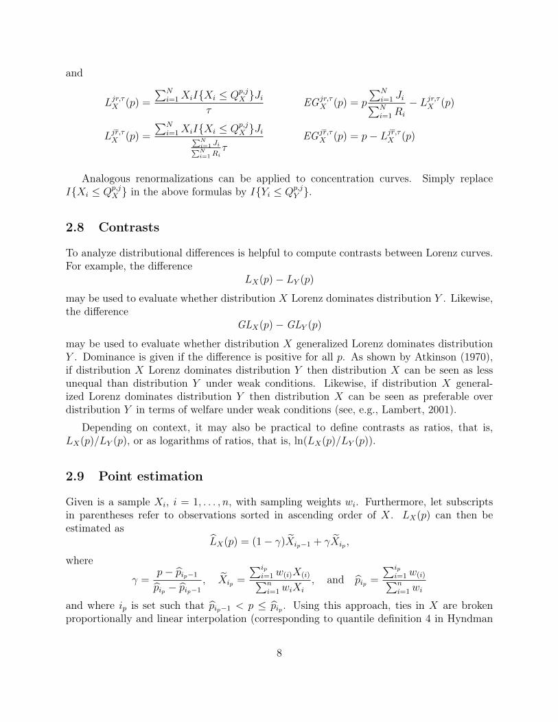
Analogous renormalizations can be applied to concentration curves. Simply replaceI{Xi Q

p,jX } in the above formulas by I{Yi Q

p,jY }.

2.8 Contrasts

To analyze distributional differences is helpful to compute contrasts between Lorenz curves.For example, the difference

LX(p)� LY (p)

may be used to evaluate whether distribution X Lorenz dominates distribution Y . Likewise,the difference

GLX(p)�GLY (p)

may be used to evaluate whether distribution X generalized Lorenz dominates distributionY . Dominance is given if the difference is positive for all p. As shown by Atkinson (1970),if distribution X Lorenz dominates distribution Y then distribution X can be seen as lessunequal than distribution Y under weak conditions. Likewise, if distribution X general-ized Lorenz dominates distribution Y then distribution X can be seen as preferable overdistribution Y in terms of welfare under weak conditions (see, e.g., Lambert, 2001).

Depending on context, it may also be practical to define contrasts as ratios, that is,LX(p)/LY (p), or as logarithms of ratios, that is, ln(LX(p)/LY (p)).

2.9 Point estimation

Given is a sample Xi, i = 1, . . . , n, with sampling weights wi. Furthermore, let subscriptsin parentheses refer to observations sorted in ascending order of X. LX(p) can then beestimated as

bLX(p) = (1� �) eXip�1 + �

eXip ,

where

� =p� bpip�1

bpip � bpip�1,

eXip =

Pipi=1 w(i)X(i)Pni=1 wiXi

, and bpip =Pip

i=1 w(i)Pni=1 wi

and where ip is set such that bpip�1 < p bpip . Using this approach, ties in X are brokenproportionally and linear interpolation (corresponding to quantile definition 4 in Hyndman

8

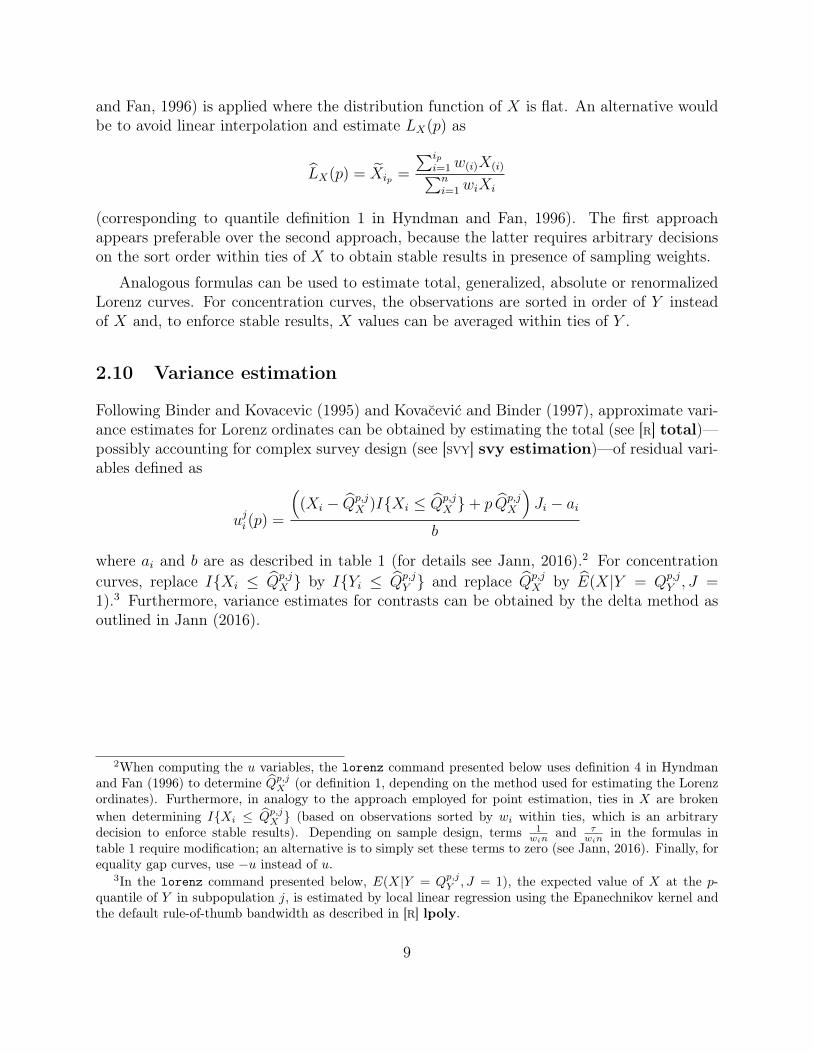
and Fan, 1996) is applied where the distribution function of X is flat. An alternative wouldbe to avoid linear interpolation and estimate LX(p) as

bLX(p) = e

Xip =

Pipi=1 w(i)X(i)Pni=1 wiXi

(corresponding to quantile definition 1 in Hyndman and Fan, 1996). The first approachappears preferable over the second approach, because the latter requires arbitrary decisionson the sort order within ties of X to obtain stable results in presence of sampling weights.

Analogous formulas can be used to estimate total, generalized, absolute or renormalizedLorenz curves. For concentration curves, the observations are sorted in order of Y insteadof X and, to enforce stable results, X values can be averaged within ties of Y .

2.10 Variance estimation

Following Binder and Kovacevic (1995) and Kovac̆ević and Binder (1997), approximate vari-ance estimates for Lorenz ordinates can be obtained by estimating the total (see [R] total)—possibly accounting for complex survey design (see [SVY] svy estimation)—of residual vari-ables defined as

u

ji (p) =

⇣(Xi � b

Q

p,jX )I{Xi b

Q

p,jX }+ p

bQ

p,jX

⌘Ji � ai

b

where ai and b are as described in table 1 (for details see Jann, 2016).2 For concentrationcurves, replace I{Xi b

Q

p,jX } by I{Yi b

Q

p,jY } and replace b

Q

p,jX by b

E(X|Y = Q

p,jY , J =

1).3 Furthermore, variance estimates for contrasts can be obtained by the delta method asoutlined in Jann (2016).

2When computing the u variables, the lorenz command presented below uses definition 4 in Hyndmanand Fan (1996) to determine bQp,j

X (or definition 1, depending on the method used for estimating the Lorenzordinates). Furthermore, in analogy to the approach employed for point estimation, ties in X are brokenwhen determining I{Xi bQp,j

X } (based on observations sorted by wi within ties, which is an arbitrarydecision to enforce stable results). Depending on sample design, terms 1

winand ⌧

winin the formulas in

table 1 require modification; an alternative is to simply set these terms to zero (see Jann, 2016). Finally, forequality gap curves, use �u instead of u.

3In the lorenz command presented below, E(X|Y = Qp,jY , J = 1), the expected value of X at the p-

quantile of Y in subpopulation j, is estimated by local linear regression using the Epanechnikov kernel andthe default rule-of-thumb bandwidth as described in [R] lpoly.

9

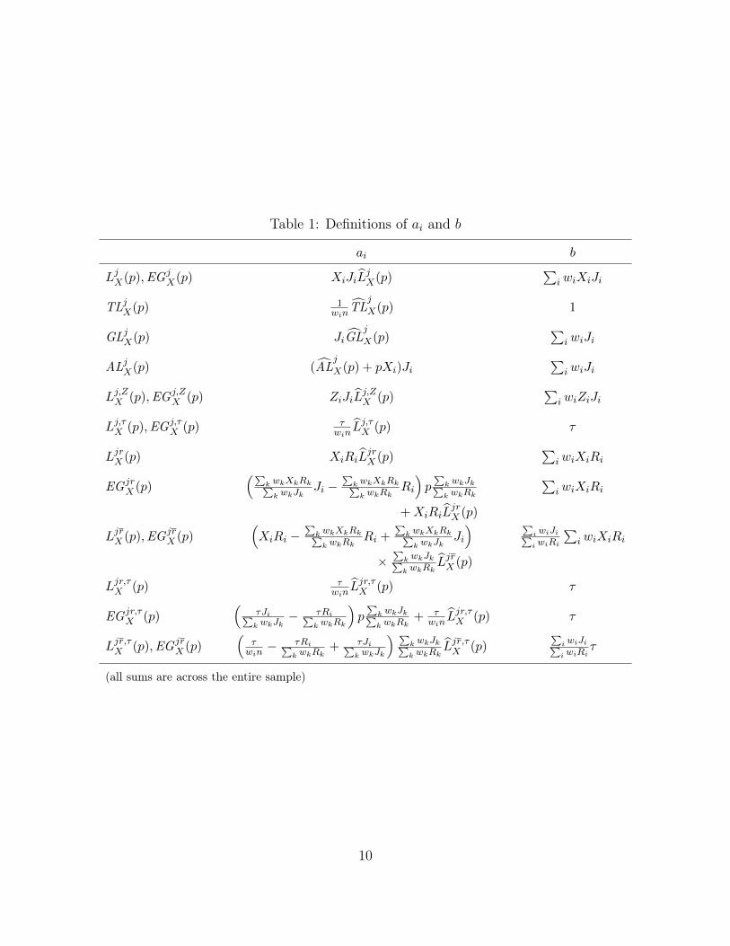
Table 1: Definitions of ai and b

ai b

LjX(p),EGj

X(p) XiJibLjX(p)

PiwiXiJi

TLjX(p) 1

wincTL

jX(p) 1

GLjX(p) JicGL

jX(p)

PiwiJi

ALjX(p) (cAL

jX(p) + pXi)Ji

PiwiJi

Lj,ZX (p),EGj,Z

X (p) ZiJibLj,ZX (p)

PiwiZiJi

Lj,⌧X (p),EGj,⌧

X (p) ⌧winbLj,⌧X (p) ⌧

LjrX (p) XiRi

bLjrX (p)

PiwiXiRi

EGjrX (p)

⇣Pk wkXkRkP

k wkJkJi �

Pk wkXkRkPk wkRk

Ri

⌘pP

k wkJkPk wkRk

+XiRibLjrX (p)

PiwiXiRi

LjrX (p),EGjr

X (p)⇣XiRi �

Pk wkXkRkPk wkRk

Ri +P

k wkXkRkPk wkJk

Ji⌘

⇥P

k wkJkPk wkRk

bLjrX (p)

Pi wiJiPi wiRi

PiwiXiRi

Ljr,⌧X (p) ⌧

winbLjr,⌧X (p) ⌧

EGjr,⌧X (p)

⇣⌧JiPk wkJk

� ⌧RiPk wkRk

⌘pP

k wkJkPk wkRk

+ ⌧winbLjr,⌧X (p) ⌧

Ljr,⌧X (p),EGjr

X (p)⇣

⌧win

� ⌧RiPk wkRk

+ ⌧JiPk wkJk

⌘ Pk wkJkPk wkRk

bLjr,⌧X (p)

Pi wiJiPi wiRi

⌧

(all sums are across the entire sample)

10

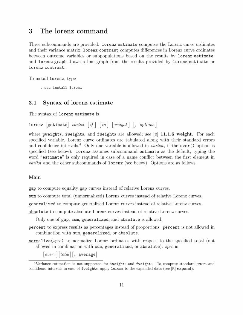
3 The lorenz command

Three subcommands are provided. lorenz estimate computes the Lorenz curve ordinatesand their variance matrix; lorenz contrast computes differences in Lorenz curve ordinatesbetween outcome variables or subpopulations based on the results by lorenz estimate;and lorenz graph draws a line graph from the results provided by lorenz estimate orlorenz contrast.

To install lorenz, type

. ssc install lorenz

3.1 Syntax of lorenz estimate

The syntax of lorenz estimate is

lorenz

⇥estimate

⇤varlist

⇥if⇤ ⇥

in⇤ ⇥

weight⇤ ⇥

, options⇤

where pweights, iweights, and fweights are allowed; see [U] 11.1.6 weight. For eachspecified variable, Lorenz curve ordinates are tabulated along with their standard errorsand confidence intervals.4 Only one variable is allowed in varlist , if the over() option isspecified (see below). lorenz assumes subcommand estimate as the default; typing theword “estimate” is only required in case of a name conflict between the first element invarlist and the other subcommands of lorenz (see below). Options are as follows.

Main

gap to compute equality gap curves instead of relative Lorenz curves.sum to compute total (unnormalized) Lorenz curves instead of relative Lorenz curves.generalized to compute generalized Lorenz curves instead of relative Lorenz curves.absolute to compute absolute Lorenz curves instead of relative Lorenz curves.

Only one of gap, sum, generalized, and absolute is allowed.percent to express results as percentages instead of proportions. percent is not allowed in

combination with sum, generalized, or absolute.normalize(spec) to normalize Lorenz ordinates with respect to the specified total (not

allowed in combination with sum, generalized, or absolute). spec is⇥over:

⇤⇥total

⇤⇥, average

⇤

4Variance estimation is not supported for iweights and fweights. To compute standard errors andconfidence intervals in case of fweights, apply lorenz to the expanded data (see [R] expand).

11

where over may be. the subpopulation at hand (the default)# the subpopulation identified by value ### the #th subpopulationtotal the total across all subpopulations

and total may be. the total of the variable at hand (the default)* the total of the sum across all analyzed outcome variablesvarlist the total of the sum across the variables in varlist# a total equal to #

total specifies the variable(s) from which the total is to be computed, or sets the totalto a fixed value. If multiple variables are specified, the total across all specified variablesis used (varlist may contain external variables that are not among the list of analyzedoutcome variables). over selects the reference population from which the total is tobe computed; over is only allowed if the over() option has been specified (see below).Suboption average causes subpopulation sizes (sum of weights) to be taken into accountso that the results are relative to the average outcome in the reference population; thisis only relevant if over is provided.

gini to report the Gini coefficients or concentration indices of the distributions (for compu-tational details see Jann, 2016).

Percentiles

nquantiles(#) to specify the number of (equally spaced) percentiles to be used to de-termine the Lorenz ordinates (plus an additional point at the origin). The default isnquantiles(20). This is equivalent to typing percentiles(0(5)100).

percentiles(numlist) to specify, as percentages, the percentiles for which the Lorenzordinates are to be computed. The numbers in numlist must be within 0 and 100.Shorthand conventions as described in [U] 11.1.8 numlist may be applied. For exam-ple, to compute Lorenz ordinates from 0 to 100% in steps of 1 percentage point, typepercentiles(0(1)100). The numbers provided in percentiles() do not need to beequally spaced and do not need to cover the whole distribution. For example, to fo-cus on the top 10% and use an increased resolution for the top 1% you could typepercentiles(90(1)98 99(0.1)100).

pvar(pvar) to compute concentration curves with respect to variable pvar .step to determine the Lorenz ordinates from the step function of cumulative outcomes. The

default is to employ linear interpolation in regions where the step function is flat.

12

Over

over(varname) to repeat results for each subpopulation defined by the values of varname.total to report additional overall results across all subpopulations. total is only allowed if

over() is specified.

Contrast/Graph

contrast(spec) to compute differences in Lorenz ordinates between outcome variables orbetween subpopulations. spec is⇥base

⇤⇥, ratio lnratio

⇤

where base is the name of the outcome variable or the value of the subpopulation tobe used as base for the contrasts. If base is omitted, adjacent contrasts across outcomevariables or subpopulations are computed (or contrasts with respect to the total if totalresults across subpopulations have been requested).Use suboption ratio to compute contrasts as ratios or suboption lnratio to computecontrasts as logarithms of ratios. The default is to compute contrasts as differences.

graph

⇥(options)

⇤to draw a line graph of the results. options are as described for

lorenz graph below.

SE/SVY

vce(vcetype) to determine how standard errors and confidence intervals are computed wherevcetype may be:

analytic

cluster clustvarbootstrap

⇥, bootstrap_options

⇤

jackknife

⇥, jackknife_options

⇤

analytic is the default. See [R] bootstrap and [R] jackknife for bootstrap_options andjackknife_options , respectively.

svy

⇥(subpop)

⇤for taking the survey design as set by svyset into account; see [SVY] svyset.

Specify subpop to restrict survey estimation to a subpopulation, where subpop is⇥varname

⇤⇥if⇤

The subpopulation is defined by observations for which varname 6= 0 and for whichthe if condition is met. See [SVY] subpopulation estimation for more information onsubpopulation estimation.The svy option is only allowed if the variance estimation method set by svyset is Taylorlinearization (the default). For other variance estimation methods the usual svy prefix

13

command can be used; see [SVY] svy. For example, type “svy brr: lorenz ...” to useBRR variance estimation. lorenz does not allow the svy prefix for Taylor linearizationdue to technical reasons. This is why the svy option is provided.

nose to suppress the computation of standard errors and confidence intervals. Use the nose

option to speed-up computations, for example, when applying a prefix command thatemploys replication techniques for variance estimation, such as, e.g., [SVY] svy jackknife.Option nose is not allowed together with vce() or svy.

Reporting

level(#) to set the level of confidence intervals; see [R] level.noheader to suppress the output header, notable to suppress the coefficient table, and

nogtable to suppress the table containing Gini coefficients.display_options such as cformat() or coeflegend to format the coefficient table. See

[R] estimation options.

3.2 Syntax of lorenz contrast

lorenz contrast computes differences in Lorenz ordinates between outcome variables orsubpopulations. It requires results from lorenz estimate to be in memory, which will bereplaced by the results from lorenz contrast.5 The syntax is

lorenz contrast

⇥base

⇤ ⇥, options

⇤

where base is the name of the outcome variable or the value of the subpopulation to be usedas base for the contrasts. If base is omitted, lorenz contrast computes adjacent contrastsacross outcome variables or subpopulations (or contrasts with respect to the total if totalresults across subpopulations have been requested). Options are:ratio to compute contrasts as ratios instead of differences.lnratio to compute contrasts as logarithms of ratios instead of differences.graph

⇥(options)

⇤to draw a line graph of the results. options are as described for

lorenz graph below.display_options such as cformat() or coeflegend to format the coefficient table. See

[R] estimation options.5Alternatively, to compute the contrasts directly, you may apply the contrast() option to

lorenz estimate (see above).

14

3.3 Syntax of lorenz graph

lorenz graph draws a line diagram of Lorenz curves or Lorenz curve contrasts. It requiresresults from lorenz estimate or lorenz contrast to be in memory.6 The syntax is

lorenz graph

⇥, options

⇤

where the options are as follows.

Main

proportion to scale the population axis as proportion (0 to 1). The default is to scale theaxis as percentage (0 to 100).

nodiagonal to omit the equal distribution diagonal that is included by default if graph-ing relative Lorenz or concentration curves. No equal distribution diagonal is includedif graphing equality gap curves or total, generalized, or absolute Lorenz/concentrationcurves or if graphing contrasts.

diagonal(options) to affect the rendition of the equal distribution diagonal. options are asdescribed in [G] line_options.

keep(list) to select and order the results to be included as separate subgraphs, where listis a list of the names of the outcome variables or the values of the subpopulations tobe included. list may also contain total for the overall results if overall results wererequested. Furthermore, you may use elements such as #1, #2, #3, . . . to refer to the 1st,2nd, 3rd, . . . outcome variable or subpopulation.

prange(min max) to restrict the range of the points to be included in the graph. Pointswhose abscissae lie outside min and max will be discarded. min and max must bewithin [0,100]. For example, to include only the upper half of the distribution, typeprange(50 100).

gini(%fmt) to set the format for the Gini coefficients included in the subgraph or legendlabels, or nogini to suppresses the Gini coefficients. These options are only relevant ifthe gini option has been specified when calling lorenz estimate. The default formatis %9.3g; see [R] format.

Labels/rendering

connect_options to affect the rendition of the plotted lines; see [G] connect_options.labels("label 1" "label 2" . . .) to specify custom labels for the subgraphs of the outcome

variables or subpopulations.6You may also draw the graph directly by applying the graph() option to lorenz estimate or

lorenz contrast (see above).

15

byopts(byopts) to determine how subgraphs are combined; see [G] by_option.overlay to include results from multiple outcome variables or subpopulations in the same

plot instead of creating subgraphs.o#(options) to affect the rendition of the line of the #th outcome variable or subpopulation

if overlay has been specified. For example, type o2(lwidth(*2)) to increase the linewidth for the second outcome variable or subpopulation. options are:

connect_options rendition of the plotted line (see [G] connect_options)⇥no

⇤ci whether to draw the confidence interval

ciopts(options) rendition of the confidence interval (see below)

Confidence intervals

level(#) to specify the confidence level, as a percentage, for confidence intervals. Thedefault is the level that has been used when running lorenz estimate. level() cannotbe used together with ci(bc), ci(bca), or ci(percentile).

ci(citype) to choose the type of confidence intervals to be plotted for results that have beencomputed using the bootstrap technique. citype may be normal (normal-based CIs; thedefault), bc (bias-corrected CIs) bca (bias-corrected and accelerated CIs) percentile

(percentile CIs). bca is only available if BCa confidence intervals have been requestedwhen running lorenz estimate (see [R] bootstrap).

ciopts(options) to affect the rendition of the plotted confidence areas. options are asdescribed in [G] area_options.

noci to omit confidence intervals from the plot.

Standard twoway options

addplot() to add other plots to the generated graph; see [G] addplot_option.twoway_options to affect the overall look of the graph, manipulate the legend, set titles, add

lines, etc.; see [G] twoway_options.

16

4 Examples

4.1 Basic application

By default, lorenz computes relative Lorenz curves on a regular-grid of 20 equally spacedpoints across the population (plus a point at the origin). The following example shows theresults for wages in the 1988 extract of the NLSW data shipped with Stata:

. sysuse nlsw88(NLSW, 1988 extract)

. lorenz estimate wage

L(p) Number of obs = 2,246

wage Coef. Std. Err. [95% Conf. Interval]

0 0 (omitted)5 .015106 .0004159 .0142904 .0159216

10 .0342651 .0007021 .0328882 .03564215 .0558635 .0010096 .0538836 .057843420 .0801846 .0014032 .0774329 .082936325 .1067687 .0017315 .1033732 .110164230 .1356307 .0021301 .1314535 .139807835 .1670287 .0025182 .1620903 .17196740 .2005501 .0029161 .1948315 .206268745 .2369209 .0033267 .2303971 .243444750 .2759734 .0037423 .2686347 .283312155 .3180215 .0041626 .3098585 .326184460 .3633071 .0045833 .3543191 .37229565 .4125183 .0050056 .4027021 .422334570 .4657641 .0054137 .4551478 .476380475 .5241784 .0058003 .5128039 .535552980 .5880894 .0062464 .5758401 .600338885 .6577051 .0066148 .6447333 .670676990 .7346412 .0068289 .7212497 .748032895 .8265786 .0062687 .8142856 .8388716

100 1 . . .

The standard errors for the first point and the last point are zero because these Lorenzordinates are 0 and 1 by definition. This is why Stata flags the first point as “omitted” andprints missing for the standard error and the confidence interval of the last point.

To graph the estimated lorenz curve, type:

. lorenz graph, aspectratio(1) xlabel(, grid)

17

0.2

.4.6

.81

cum

ulat

ive

outc

ome

prop

ortio

n

0 20 40 60 80 100population percentage

L(p) 95% CI

The aspectratio(1) option has been added to enforce a quadratic plot region andxlabel(, grid) has been added to include vertical grid lines. Note that, instead of applyinglorenz graph as a separate command, you can also directly specify the graph option withlorenz estimate (see next example).

The default for lorenz is to use a regular grid of evaluation points across the wholedistribution. To use an irregular grid or to cover just a part of the distribution, use thepercentiles() option. The following example focusses on the upper 20% and uses a differentstep size towards the tail of the distribution.

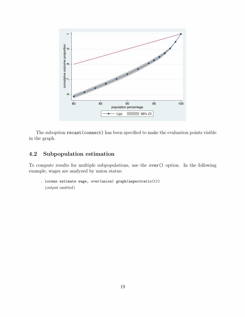
. lorenz estimate wage, percentiles(80(2)94 95(1)100) graph(recast(connect))

L(p) Number of obs = 2,246

wage Coef. Std. Err. [95% Conf. Interval]

80 .5880894 .0062464 .5758401 .600338882 .6151027 .0063755 .6026003 .627605184 .6432933 .0065449 .6304586 .656128186 .672506 .006651 .6594633 .685548788 .70278 .0067917 .6894613 .716098790 .7346412 .0068289 .7212497 .748032892 .7684646 .0067952 .7551391 .781790194 .806114 .0064727 .7934209 .818807195 .8265786 .0062687 .8142856 .838871696 .8485922 .0060386 .8367504 .86043497 .8730971 .0051329 .8630314 .883162998 .9046081 .0027287 .899257 .909959199 .9486493 .000697 .9472826 .9500161

100 1 . . .

18

.6.7

.8.9

1cu

mul

ativ

e ou

tcom

e pr

opor

tion

80 85 90 95 100population percentage

L(p) 95% CI

The suboption recast(connect) has been specified to make the evaluation points visiblein the graph.

4.2 Subpopulation estimation

To compute results for multiple subpopulations, use the over() option. In the followingexample, wages are analyzed by union status:

. lorenz estimate wage, over(union) graph(aspectratio(1))

(output omitted )

19

0.5

1

0 50 100 0 50 100

nonunion union

L(p) 95% CI

cum

ulat

ive

outc

ome

prop

ortio

n

population percentage

By default, lorenz places results for the subpopulations in separate subgraphs. Tocombine the results in a single plot, use the overlay option:

. lorenz graph, overlay aspectratio(1) xlabel(, grid)

0.2

.4.6

.81

cum

ulat

ive

outc

ome

prop

ortio

n

0 20 40 60 80 100population percentage

nonunion union

20

4.3 Contrasts and Lorenz dominance

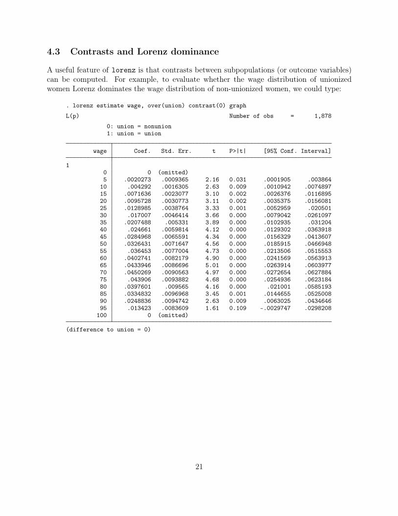
A useful feature of lorenz is that contrasts between subpopulations (or outcome variables)can be computed. For example, to evaluate whether the wage distribution of unionizedwomen Lorenz dominates the wage distribution of non-unionized women, we could type:

. lorenz estimate wage, over(union) contrast(0) graph

L(p) Number of obs = 1,878

0: union = nonunion1: union = union

wage Coef. Std. Err. t P>|t| [95% Conf. Interval]

10 0 (omitted)5 .0020273 .0009365 2.16 0.031 .0001905 .003864

10 .004292 .0016305 2.63 0.009 .0010942 .007489715 .0071636 .0023077 3.10 0.002 .0026376 .011689520 .0095728 .0030773 3.11 0.002 .0035375 .015608125 .0128985 .0038764 3.33 0.001 .0052959 .02050130 .017007 .0046414 3.66 0.000 .0079042 .026109735 .0207488 .005331 3.89 0.000 .0102935 .03120440 .024661 .0059814 4.12 0.000 .0129302 .036391845 .0284968 .0065591 4.34 0.000 .0156329 .041360750 .0326431 .0071647 4.56 0.000 .0185915 .046694855 .036453 .0077004 4.73 0.000 .0213506 .051555360 .0402741 .0082179 4.90 0.000 .0241569 .056391365 .0433946 .0086696 5.01 0.000 .0263914 .060397770 .0450269 .0090563 4.97 0.000 .0272654 .062788475 .043906 .0093882 4.68 0.000 .0254936 .062318480 .0397601 .009565 4.16 0.000 .021001 .058519385 .0334832 .0096968 3.45 0.001 .0144655 .052500890 .0248836 .0094742 2.63 0.009 .0063025 .043464695 .013423 .0083609 1.61 0.109 -.0029747 .0298208

100 0 (omitted)

(difference to union = 0)

21

0.0

2.0

4.0

6di

ffere

nce

in L

(p)

0 20 40 60 80 100population percentage

difference in L(p) 95% CI

As is evident, the Lorenz curve of wages of unionized women lies above the Lorenz curve ofwages of non-unionized women. Hence it appears save to conclude that the wage distributionof non-unionized women is more unequal than the wage distribution of unionized women.

Lorenz dominance does not necessarily imply that one distribution is preferable overthe other from a welfare perspective. To evaluate welfare ordering, it is useful to analyzegeneralized Lorenz dominance. The following example shows the generalized Lorenz curvesof wages of unionized and non-unionized women:

. lorenz estimate wage, over(union) generalized graph(overlay)

(output omitted )

22

02

46

810

cum

ulat

ive

mea

n

0 20 40 60 80 100population percentage

nonunion union

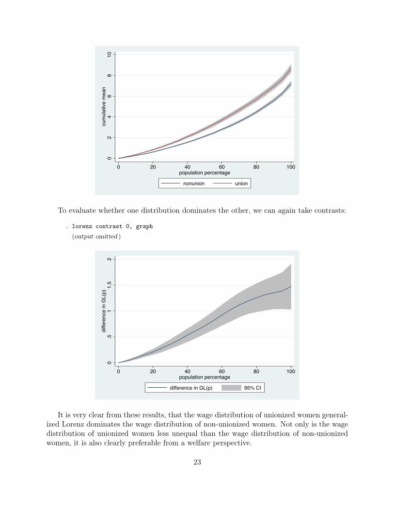
To evaluate whether one distribution dominates the other, we can again take contrasts:

. lorenz contrast 0, graph

(output omitted )

0.5

11.

52

diffe

renc

e in

GL(

p)

0 20 40 60 80 100population percentage

difference in GL(p) 95% CI

It is very clear from these results, that the wage distribution of unionized women general-ized Lorenz dominates the wage distribution of non-unionized women. Not only is the wagedistribution of unionized women less unequal than the wage distribution of non-unionizedwomen, it is also clearly preferable from a welfare perspective.

23

4.4 Concentration curves and renormalization

Concentration curves are used to illustrate how one variables is distributed across the popu-lation ranked by another variable. As an example, consider the following household datasetthat contains information on transfer income, capital income, and earnings. We may use thepvar() option to analyze how transfers and capital rents are distributed across households,while ranking households by earnings:

. use lorenz_exampledata

. summarize

Variable Obs Mean Std. Dev. Min Max

earnings 6,007 94673.66 72285.96 0 1965925capincome 6,007 8346.58 50226.91 0 2374227transfers 6,007 6375.284 15838.54 0 239408

. lorenz transfers capincome, pvar(earnings)> graph(overlay aspectratio(1) xlabels(, grid) legend(cols(1))> ciopts(recast(rline) lp(dash)))

(output omitted )

0.2

.4.6

.81

cum

ulat

ive

outc

ome

prop

ortio

n

0 20 40 60 80 100population percentage (ordered by earnings)

transferscapincome

We see, as expected, that the concentration curve of transfers lies above the equal dis-tribution line. That is, transfers benefit households with low earnings. For example, thebottom 50% of households in the earnings distribution receive about 80% of all transfers.Capital income, however, is skewed towards high earning households (the bottom 50% ofhouseholds in the earnings distribution receive about 25% of all capital income).

Furthermore, the normalize() option can be use together with pvar() to subdivide theLorenz curve of total income by income factors:

24

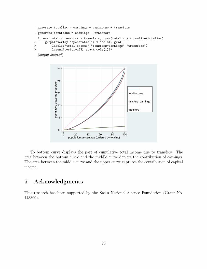
. generate totalinc = earnings + capincome + transfers

. generate earntrans = earnings + transfers

. lorenz totalinc earntrans transfers, pvar(totalinc) normalize(totalinc)> graph(overlay aspectratio(1) xlabels(, grid)> labels("total income" "tansfers+earnings" "transfers")> legend(position(3) stack cols(1)))

(output omitted )0

.2.4

.6.8

1cu

mul

ativ

e ou

tcom

e pr

opor

tion

0 20 40 60 80 100population percentage (ordered by totalinc)

total income

tansfers+earnings

transfers

To bottom curve displays the part of cumulative total income due to transfers. Thearea between the bottom curve and the middle curve depicts the contribution of earnings.The area between the middle curve and the upper curve captures the contribution of capitalincome.

5 Acknowledgments

This research has been supported by the Swiss National Science Foundation (Grant No.143399).

25

References

Abdelkrim, A. 2005. clorenz: module to estimate Lorenz and concentra-tion curves. Statistical Software Components S456515. Available fromhttp://ideas.repec.org/c/boc/bocode/s456515.html.

Atkinson, A. B. 1970. On the measurement of inequality. Journal of Economic Theory 2:244–263.

Azevedo, J. P., and S. Franco. 2006. alorenz: Stata module to produce Pen’s Parade, Lorenzand Generalised Lorenz curve. Statistical Software Components S456749. Available fromhttp://ideas.repec.org/c/boc/bocode/s456749.html.

Binder, D. A., and M. S. Kovacevic. 1995. Estimating Some Measures of Income Inequal-ity from Survey Data: An Application of the Estimating Equations Approach. SurveyMethodology 21(2): 137–145.

Bishop, J. A., K. V. Chow, and J. P. Formby. 1994. Testing for Marginal Changes in IncomeDistributions with Lorenz and Concentration Curves. International Economic Review35(2): 479–488.

Cowell, F. A. 2000. Measurement of Inequality. In Handbook of Income Distribution, ed.A. B. Atkinson and F. Bourguignon, vol. 1, 87–166. Amsterdam: Elsevier.

———. 2011. Measuring Inequality. 2nd ed. Oxford: Oxford University Press.

Hao, L., and D. Q. Naiman. 2010. Assessing Inequality. Thousand Oaks, CA: Sage.

Hyndman, R. J., and Y. Fan. 1996. Sample Quantiles in Statistical Packages. The AmericanStatistician 50(4): 361–365.

Jann, B. 2016. Assessing inequality using percentile shares. The Stata Journal 16(2): 264–300.

Jenkins, S. P. 2006. svylorenz: Stata module to derive distribution-free variance es-timates from complex survey data, of quantile group shares of a total, cumula-tive quantile group shares. Statistical Software Components S456602. Available fromhttp://ideas.repec.org/c/boc/bocode/s456602.html.

Jenkins, S. P., and P. Van Kerm. 1999. sg107: Generalized Lorenz curves and related graphs.Stata Technical Bulletin 48: 25–29.

Kovac̆ević, M. S., and D. A. Binder. 1997. Variance Estimation for Measures of IncomeInequality and Polarization – The Estimating Equations Approach. Journal of OffcialStatistics 13(1): 41–58.

26

Lambert, P. J. 2001. The distribution and redistribution of income. A mathematical analysis.3rd ed. Manchester: Manchester University Press.

Lorenz, M. O. 1905. Methods of Measuring the Concentration of Wealth. Publications ofthe American Statistical Association 9(70): 209–219.

Moyes, P. 1987. A new concept of Lorenz domination. Economics Letters 23(2): 203–207.

Shorrocks, A. F. 1983. Ranking income distributions. Economica 50(197): 3–17.

Van Kerm, P., and S. P. Jenkins. 2001. Generalized Lorenz curves and related graphs: anupdate for Stata 7. The Stata Journal 1(1): 107–112.

27