Estimating Lorenz Curves Using a Dirichlet Distribution Duangkamon Chotikapanich

Department of Economics, Curtin University of Technology, Perth, WA 6845 (chotikapanichd@cbs.curtin.edu.au)

William E. Griffiths Department of Economics, University of Melbourne, Vic 3010, Australia

(b.griffiths@unimelb.edu.au)

Abstract The Lorenz curve relates the cumulative proportion of income to the cumulative

proportion of population. When a particular functional form of the Lorenz curve

is specified it is typically estimated by linear or nonlinear least squares,

estimation techniques that have good properties when the error terms are

independently and normally distributed. Observations on cumulative proportions

are clearly neither independent nor normally distributed. This paper proposes and

applies a new methodology that recognizes the cumulative proportional nature of

the Lorenz curve data by assuming that the income proportions are distributed as

a Dirichlet distribution. Five Lorenz-curve specifications are used to demonstrate

the technique. Maximum likelihood estimates under the Dirichlet distribution

assumption provide better-fitting Lorenz curves than nonlinear least squares and

another estimation technique that has appeared in the literature.

Keywords: Gini coefficient; maximum likelihood estimation.

2

1. INTRODUCTION

The Lorenz curve is one of the most important tools upon which the measurement

of income inequality is based. For a given economy or region, it relates the

cumulative proportion of income to the cumulative proportion of population, after

ordering the population according to increasing level of income. A number of

approaches to Lorenz curve estimation have been adopted. In one approach, a

particular assumption about the statistical distribution of income is made, the

parameters of this income distribution are estimated, and a Lorenz curve

consistent with the distributional assumption, and consistent with the parameter

estimates for that distribution, is obtained. See, for example, McDonald (1984)

and McDonald and Xu (1995). Ryu and Slottje (1996) suggest another approach.

They approximate the Lorenz curve from any income distribution by expanding

the inverse distribution function in terms of (a) an exponential polynomial series

and (b) a sequence of Bernstein polynomial functions. When micro-data are

available, nonparameteric estimation of the Lorenz curve and related inequality

measures is possible. See, for example, Beach and Davidson (1983), Gastwirth

and Gail (1985), and Bishop et al (1989). An alternative approach, more suited to

grouped data, is to specify a particular functional form for the Lorenz curve and

estimate it directly. It is this approach that is the focus of this paper.

Early breakthroughs on Lorenz curve estimation were those of Gastwirth (1972)

and Kakwani and Podder (1973, 1976). Kakwani and Podder recognized the

multinomial nature of grouped data and used a Lorenz curve specification that,

after transformation, could be placed in an approximate linear model framework.

3

Other specifications have typically been estimated by linear or nonlinear least

squares (Kakwani 1980, Basmann et al 1990, Chotikapanich 1993). Such

exercises are useful for fitting Lorenz curves, but, because the covariance matrix

estimates they provide are only relevant for independent normally distributed

errors, they do not provide a basis for inference about Lorenz curve parameters or

any inequality measures derived from them. Clearly, observations on cumulative

proportions, or even their logarithms if such a transformation is convenient, will

be neither independent nor normally distributed. Sarabia et al (1999) overcome

this problem by suggesting a distribution-free method of estimation. Suppose that

a Lorenz curve has n unknown parameters, and that M observations on the

cumulative proportions are available. They find a set of parameter estimates for

each of the

= n

MK subsets of n observations. Since each of the subsets yields

n equations in n unknown parameters, a set of parameter estimates is obtained by

solving these equations. The medians of the sets of parameter estimates are

recommended as the final set of estimates. No distribution theory is available for

this procedure, but the authors do provide some bootstrap standard errors.

An alternative way to proceed, and the approach adopted in this paper, is to

choose a distributional assumption that is consistent with the proportional nature

of the data and to pursue maximum likelihood estimation. A suitable distribution

is the Dirichlet distribution. It is a multivariate distribution for a vector of random

variables that are shares that sum to unity. By relating the parameters of the

Dirichlet distribution to Lorenz curve differences, we can accommodate the

cumulative proportional nature of the Lorenz curve data, and set up a likelihood

function dependent on the unknown parameters of the Lorenz curve. A similar

4

approach was adopted by Woodland (1979) for estimation of share equations that

arise in demand and production theory. To further motivate the choice of a

Dirichlet distribution, note that, with random sampling, the number of households

in each of a number of income classes can be viewed as an observation from the

multinomial distribution (Aigner and Goldberger 1970, Kakwani and Podder

1973). Furthermore, by using a transformation from cell numbers to cell

proportions, the multinomial distribution can be approximated by a Dirichlet

distribution (Johnson 1960, Johnson and Kotz 1969, p.285). Thus, the Dirichlet

distribution is a reasonable choice for share data, irrespective of the original

income distribution from which the observations were drawn. The choice of a

Dirichlet distribution for income shares is much less arbitrary than choosing a

specific income distribution. In addition, the number of recognized multivariate

distributions that are directly applicable to share data is very limited. Apart from

the Dirichlet distribution, only two other possibly-relevant generalized beta

distributions are described in Johnson and Kotz (1972). These facts and the

general lack of recognition of the share nature of the data in much of the literature

on Lorenz curve estimation, make the Dirichlet distribution a useful alternative to

pursue.

In Section 2, we outline the distributional assumptions and how they relate to

Lorenz curve estimation. The likelihood function for a set of unknown Lorenz

curve parameters is derived. To illustrate our suggested techniques we use data

on Sweden and Brazil considered earlier by Shorrocks (1983) and revisited by

Sarabia et al (1999). These data are described in Section 3; five different Lorenz

functions that we use in the empirical work are presented. The results are given

5

and discussed in Section 4. Several questions are investigated. To examine

whether the results are sensitive to the chosen estimation technique we compare

our estimates and their standard errors to those obtained by Sarabia et al (1999),

and those obtained using nonlinear least squares. Since Lorenz-curve estimation

is usually a first step towards estimating inequality, maximum likelihood (ML)

and nonlinear least squares estimates for the Gini coefficient are obtained for

each Lorenz-curve specification. Finally, we examine which estimation technique

leads to the best fitting Lorenz curve.

2. MODELS, ASSUMPTIONS AND ESTIMATION

Suppose we have available observations on cumulative proportions of population

( Mπππ ,,, 21 … with 1=πM ) and corresponding cumulative proportions of

income ( Mηηη ,,, 21 … with 1=ηM ) obtained after ordering population units

according to increasing income. We wish to use these observations to estimate a

parametric version of a Lorenz curve that we write as );( βπ=η L where β is an

)1( ×n vector of unknown parameters. Clearly, one would not expect all data

points to lie exactly on the curve );( βπ=η ii L . It seems reasonable to assume,

however, that conditional on the population proportions iπ , the income shares

1−η−η= iiiq are random variables with means

);();()()()( 11 βπ−βπ=η−η= −− iiiii LLEEqE (1)

Our proposal is to also assume )',,,( 21 Mqqqq …= follows a Dirichlet

distribution which is a distribution consistent with the share nature of the random

vector q. The probability density function (pdf) for the Dirichlet distribution is

given by

6

112

11

21

21 21

)()()()()|( −α−α−α

αΓαΓαΓα++α+αΓ=α M

MM

M qqqqf ……" (2)

where )',,,( 21 Mααα=α … are the parameters of the pdf and (.)Γ is the gamma

function. By relating the iα to the Lorenz function, we can find a pdf for q which

has the mean given in equation (1) and which is a function of the Lorenz curve

parameters. Working in this direction, we set

[ ]);();( 1 βπ−βπλ=α −iii LL (3)

where λ is an additional unknown parameter. This definition for iα gives the

desired result because the mean of the Dirichlet distribution is given by

[ ]

∑=

−

−

βπ−βπλ

βπ−βπλ=

α++α+αα=

M

iii

ii

M

ii

LL

LL

qE

11

1

21

)];();([

);();(

)("

);();( 1 βπ−βπ= −ii LL (4)

since 1);( =βπML and 0);( 0 =βπL . We can now write the pdf for q as

∏= −

−βπ−βπλ

βπ−βπλΓλΓ=θ

−M

i ii

LLi

LLqqf

ii

1 1

1)];();([

)]);();([()()|(

1

(5)

where '),'( λβ=θ .

The variances and covariances between the shares are given by (Johnson and

Kotz, 1972, p.231-234)

1

)](1)[()var(+λ−= ii

iqEqEq (6)

7

1

)()(),cov(

+λ−= ji

jiqEqE

qq (7)

Thus, the income shares are correlated, with correlations given by

2/1

)](1)][(1[)()(

−−−=

ji

jiij qEqE

qEqEr (8)

Since the variances depend on )( iqE , the shares are also heteroskedastic. The

parameter λ acts as an inverse variance parameter. The larger the value of λ , the

better the fit of the Lorenz curve to the data.

The maximum likelihood estimate for θ can be found by maximizing the log-

likelihood function

∑

∑

=−

=−

βπ−βπλΓ−

−βπ−βπλ+λΓ=θ

M

iii

M

iiii

LL

qLLqf

11

11

)]);();([(log

log)1)];();([()(log)]|(log[

(9)

3. DATA AND LORENZ CURVES

To illustrate our suggested techniques we use income distribution data on

national samples of income recipients for a year close to 1970, for two countries:

Sweden and Brazil. These data were used by Sarabia et al (1999). They were

derived from Jain (1975) and first published in Shorrocks (1983). The data are in

the form of decile cumulative income shares. Shorrocks used the data on these

two countries as part of a group of twenty countries to examine the ranking of

income distributions given different social states. Sarabia et al (1999) used the

data to illustrate their proposed method for the estimation of Lorenz curves. The

8

data on these two countries were chosen because of their differences in the degree

of inequality in income distributions.

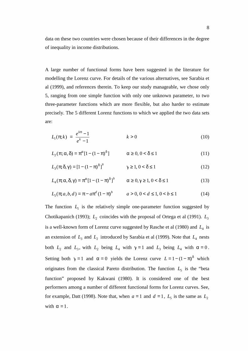
A large number of functional forms have been suggested in the literature for

modelling the Lorenz curve. For details of the various alternatives, see Sarabia et

al (1999), and references therein. To keep our study manageable, we chose only

5, ranging from one simple function with only one unknown parameter, to two

three-parameter functions which are more flexible, but also harder to estimate

precisely. The 5 different Lorenz functions to which we applied the two data sets

are:

11);(1 −

−=ππ

k

k

eekL 0>k (10)

])1(1[),;(2δα π−−π=δαπL 10,0 ≤δ<≥α (11)

γδπ−−=γδπ ])1(1[),;(3L 10,1 ≤δ<≥γ (12)

γδα π−−π=γδαπ ])1(1[),,;(4L 10,1,0 ≤δ<≥γ≥α (13)

bdadbaL )1(),,;(5 π−π−π=π 10,10,0 ≤<≤<> bda (14)

The function 1L is the relatively simple one-parameter function suggested by

Chotikapanich (1993); 2L coincides with the proposal of Ortega et al (1991). 3L

is a well-known form of Lorenz curve suggested by Rasche et al (1980) and 4L is

an extension of 3L and 2L introduced by Sarabia et al (1999). Note that 4L nests

both 2L and 3L , with 2L being 4L with 1=γ and 3L being 4L with 0=α .

Setting both 1=γ and 0=α yields the Lorenz curve δπ−−= )1(1L which

originates from the classical Pareto distribution. The function 5L is the “beta

function” proposed by Kakwani (1980). It is considered one of the best

performers among a number of different functional forms for Lorenz curves. See,

for example, Datt (1998). Note that, when 1=a and 1=d , 5L is the same as 2L

with 1=α .

9

Once a Lorenz curve has been estimated, one is usually interested in various

inequality measures that are related to it. As an example, we compute maximum

likelihood estimates for the Gini coefficients that can be derived from each of the

Lorenz functions. In each case the Gini coefficient is defined as

∫ πβπ−=1

0

);(21 dLG (15)

Alternative expressions for G can be found for some of the Lorenz curves.

However, with the exception of 1L , they still generally involve a numerical

integral. We obtain ML estimates by numerically evaluating (15) in each case

with β replaced by the ML estimate β̂ .

4. RESULTS

In addition to ML estimation using the assumption of a Dirichlet distribution, we

also estimated each function using nonlinear least squares. Because nonlinear

least squares has been popular in the literature, it is useful to compare its

estimates and standard errors to those from ML estimation. However,

conventional nonlinear least squares (NL) standard errors are computed assuming

independent identically distributed error terms, an assumption that is unrealistic

with share data. Thus, for NL standard errors we report those suggested by

Newey and West (1987). The estimates and standard errors obtained by Sarabia

et al (1999), for 2 3,L L and 4L are also reported; they provide further evidence

on the sensitivity of estimates to choice of estimation technique. However,

‘Sarabia estimates’ for 1L and 5L are not available; nor are the standard errors for

the ‘Sarabia-based’ Gini coefficient estimates for all functions.

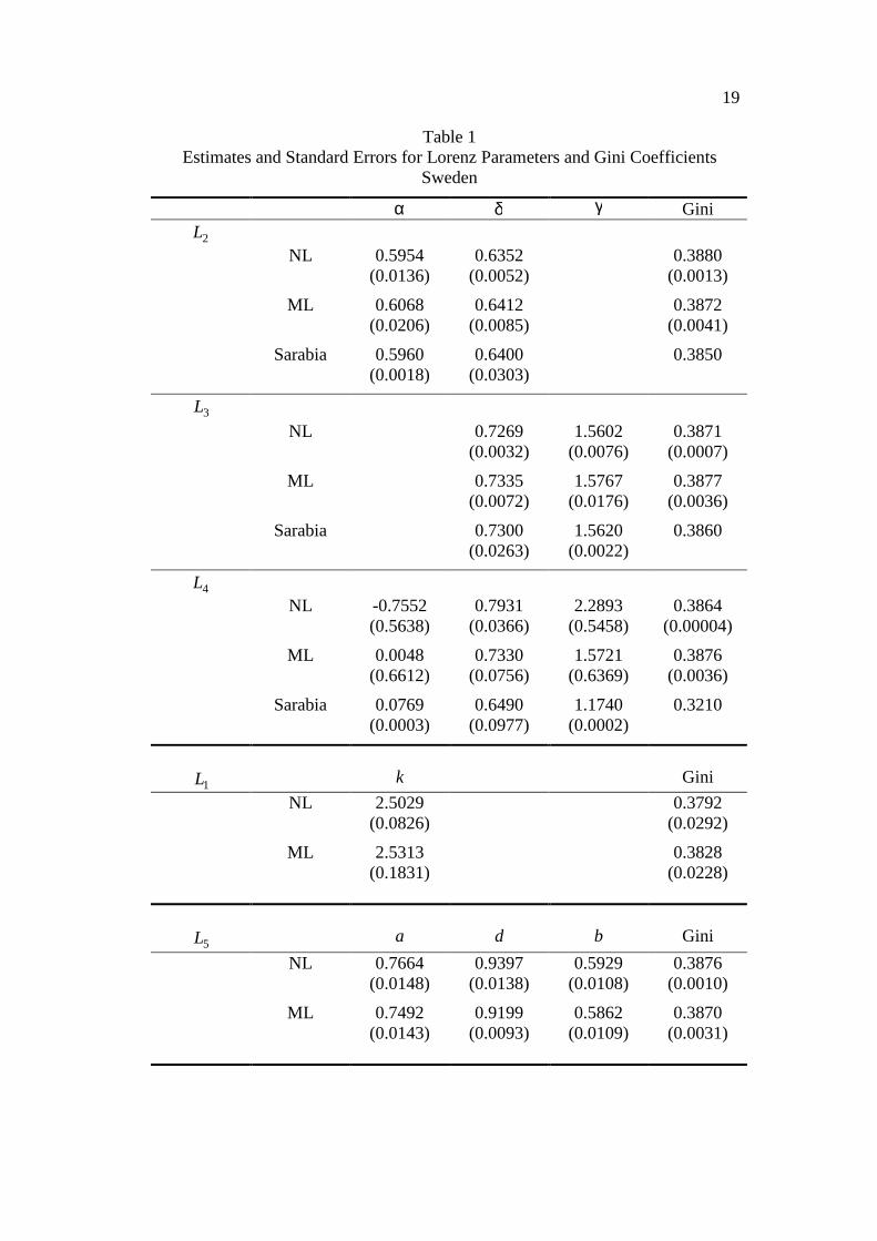
Point estimates and standard errors of the Lorenz curve parameters and the

corresponding Gini coefficients for Sweden are presented in Table 1. With the

10

exception of the function 4L , the estimates of the Lorenz parameters and the Gini

coefficient are not sensitive to the estimation technique. Nonlinear least squares,

ML and ‘Sarabia’ lead to almost identical estimates. For 4L there is considerable

variation in the Lorenz parameter estimates, and the Sarabia-estimated Gini

coefficient is noticeably different from the others. A somewhat remarkable

outcome is that, with the exception of the Sarabia et al estimate from 4L , the

point estimates of the Gini coefficient are relatively insensitive to estimation

technique and functional form specification.

[Table 1 near here]

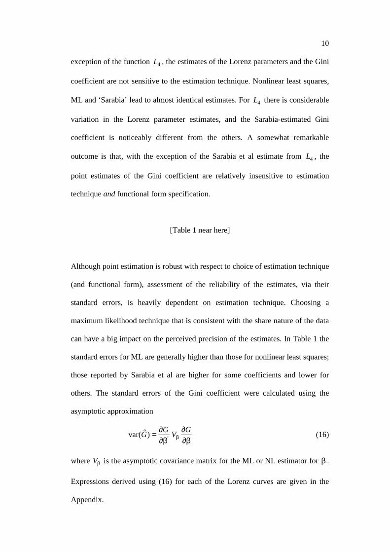
Although point estimation is robust with respect to choice of estimation technique

(and functional form), assessment of the reliability of the estimates, via their

standard errors, is heavily dependent on estimation technique. Choosing a

maximum likelihood technique that is consistent with the share nature of the data

can have a big impact on the perceived precision of the estimates. In Table 1 the

standard errors for ML are generally higher than those for nonlinear least squares;

those reported by Sarabia et al are higher for some coefficients and lower for

others. The standard errors of the Gini coefficient were calculated using the

asymptotic approximation

β∂

∂β∂

∂= βGVGG ')ˆvar( (16)

where βV is the asymptotic covariance matrix for the ML or NL estimator for β .

Expressions derived using (16) for each of the Lorenz curves are given in the

Appendix.

11

The remarks made about Sweden also hold for the estimates for Brazil given in

Table 2, with some minor exceptions. Once again, there are vastly different

estimates for 4L , confirming considerable instability in the estimation of this

function. In contrast to Sweden, estimates of the 1L parameter and corresponding

Gini coefficient are also sensitive to choice of estimation technique. The other

functions remain insensitive to choice of estimation technique. Except for 1L the

Gini coefficient estimates are insensitive with respect to both estimation

technique and choice of functional form. Despite yielding similar point estimates,

the three estimation techniques yield very different standard errors.

[Table 2 near here]

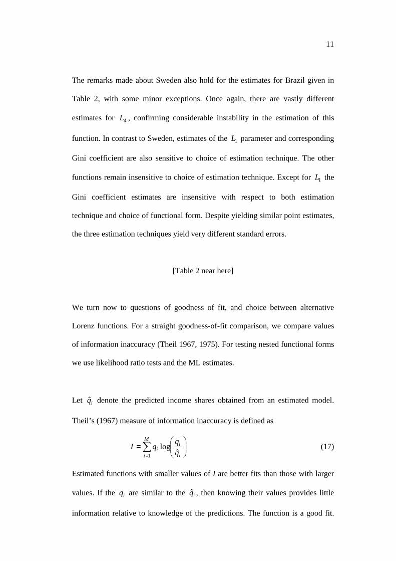
We turn now to questions of goodness of fit, and choice between alternative

Lorenz functions. For a straight goodness-of-fit comparison, we compare values

of information inaccuracy (Theil 1967, 1975). For testing nested functional forms

we use likelihood ratio tests and the ML estimates.

Let iq̂ denote the predicted income shares obtained from an estimated model.

Theil’s (1967) measure of information inaccuracy is defined as

∑=

=

M

i i

ii q

qqI1 ˆ

log (17)

Estimated functions with smaller values of I are better fits than those with larger

values. If the iq are similar to the iq̂ , then knowing their values provides little

information relative to knowledge of the predictions. The function is a good fit.

12

On the other hand, iq quite different from the iq̂ convey considerable

information, leading to a large value of I and a poor fit. The information

inaccuracy measure was computed using predictions from the nonlinear and ML

estimates, and for the Sarabia et al estimates for functions 2L , 3 4 and L L . The

outcomes are presented in Table 3.

[ Table 3 near here]

For the Swedish data, ML estimation provides a better fit than nonlinear least

squares for all functional forms. It also provides better fits than those from the

technique suggested by Sarabia et al for the functions they considered. The

differences are not great for 1 2 3, and L L L ; they are most noticeable for

4 5 and L L . The large improvement of ML over nonlinear least squares in the case

of 5L is perhaps surprising, given the apparent similarity of the two sets of

Lorenz curve estimates. A closer examination of the two sets of predictions for

this case revealed that they were not as close as one might suspect by comparing

parameter estimates. Also, nonlinear least squares led to some relatively large

over predictions that were penalised heavily by the information criterion. Finally,

it is interesting that a ranking of the relative magnitudes of the ML standard

errors for the Gini coefficient corresponds exactly to a goodness-of-fit ranking of

the ML-estimated Lorenz functions.

13

The information inaccuracies for the Brazilian data lead to the same conclusions

with two small modifications. Nonlinear least squares and ML estimation of 5L

had the same fit. Nonlinear least squares provided a better fit than ML for 1L .

To provide information about choice of functional form we examined whether

likelihood ratio tests suggested nested versions of 4L and 5L would be adequate.

The availability of these tests is one of the advantages of the maximum likelihood

methodology that we have proposed. Table 4 contains 2χ values for likelihood

ratio tests for various hypotheses. These results suggest that 3L is an acceptable

restricted version of 4L for both Sweden and Brazil. Also, 2L is an acceptable

restricted version of 4L for Sweden, but not for Brazil. Finally, a restricted

version of 2L , obtained by setting 1=α , is clearly rejected relative to the best-

fitting 5L .

[Table 4 near here.]

5. CONCLUSIONS AND SUMMARY

One way of estimating a Lorenz curve is to assume a particular distribution for

income, estimate the parameters of that distribution, and derive the corresponding

Lorenz curve. Another way is to assume a particular Lorenz curve, and estimate

its parameters. For this second approach we have suggested a distributional

assumption and a corresponding estimation technique which is consistent with

the proportional nature of Lorenz-curve data, can be used to approximate share

14

data from any income distribution, and can be employed with any Lorenz-curve

specification.

Our model and estimation technique was applied to two data sets that have been

the subject of past analyses, one for Sweden, a country with relatively low

inequality, and one for Brazil, a country with relatively high inequality. Results

were obtained for 5 different Lorenz-curve specifications. Our findings do not

necessarily carry over to other data sets and other functions. With this fact kept in

mind, we reached the following conclusions. Point estimation of the Gini

coefficient was generally insensitive to choice of distributional assumption,

estimation technique and Lorenz-curve specification. There were two exceptions

to this conclusion. One was for the function 1L applied to the Brazilian data,

using the Dirichlet distribution. The second exception was the estimate from 4L

with the Swedish data and the estimation technique of Sarabia et al. The

discrepancy obtained in this case appears to be a consequence of estimation

instability associated with this function.

Although point estimation of the Gini coefficient was robust, assessment of the

precision of estimation was not. It depended heavily on choice of functional form

and choice of estimation technique. With respect to estimation technique, we

found that ML estimation, under our proposal to use the Dirichlet distribution,

provided the best fit. Useful future work would be a Monte Carlo study to assess

whether the standard errors produced by each estimation technique are an

accurate reflection of finite-sample variability of the estimates.

15

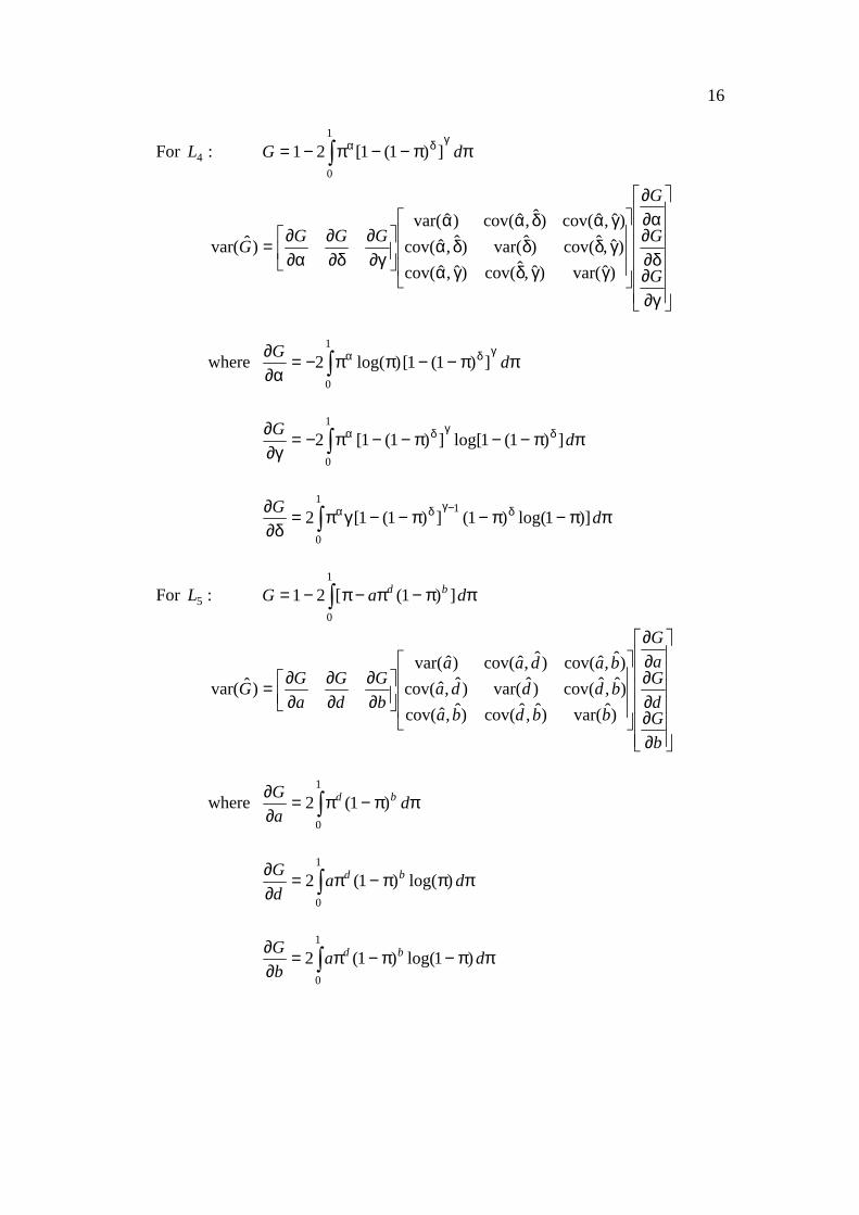
APPENDIX: EXPRESSIONS FOR VARIANCES

OF THE GINI COEFFICIENT

For 1L : )ˆvar())1(ˆ(

)1)2ˆ((2)ˆvar(2

2ˆ

22ˆ

kek

keeGk

k

−+−−=

For :2L ∫ ππ−−π−= δα1

0

])1(1[21 dG

δ∂∂

α∂∂

δδαδαα

δ∂∂

α∂∂= G

GGGG

)ˆvar()ˆ,ˆcov()ˆ,ˆcov()ˆvar()ˆvar(

where ∫ ππ−−ππ−=α∂

∂ δα1

0

])1(1[)log(2 dG

and ∫ ππ−π−π=δ∂

∂ δα1

0

)1log()1(2 dG

For :3L ∫ ππ−−−=γδ

1

0

])1(1[21 dG

γ∂∂

δ∂∂

γγδγδδ

γ∂

∂δ∂

∂= G

GGGG

)ˆvar()ˆ,ˆcov()ˆ,ˆcov()ˆvar()ˆvar(

where ∫ ππ−π−π−−γ=δ∂

∂ δ−γδ1

0

1)1log()1(])1(1[2 dG

and ∫ ππ−−π−−−=γ∂

∂ δγδ1

0

])1(1log[])1(1[2 dG

16

For :4L ∫ ππ−−π−=γδα

1

0

])1(1[21 dG

γ∂∂

δ∂∂

α∂∂

γγδγαγδδδαγαδαα

γ∂

∂δ∂

∂α∂

∂=

G

G

G

GGGG)ˆvar()ˆ,ˆcov()ˆ,ˆcov()ˆ,ˆcov()ˆvar()ˆ,ˆcov()ˆ,ˆcov()ˆ,ˆcov()ˆvar(

)ˆvar(

where ∫ ππ−−ππ−=α∂

∂ γδα1

0

])1(1[)log(2 dG

∫ ππ−−π−−π−=γ∂

∂ δγδα1

0

])1(1log[])1(1[2 dG

∫ ππ−π−π−−γπ=δ∂

∂ δ−γδα1

0

1)]1log()1(])1(1[2 dG

For :5L ∫ ππ−π−π−=1

0

])1([21 daG bd

∂∂∂∂∂∂

∂∂

∂∂

∂∂=

bGdGaG

bbdbabdddabadaa

bG

dG

aGG

)ˆvar()ˆ,ˆcov()ˆ,ˆcov()ˆ,ˆcov()ˆvar()ˆ,ˆcov()ˆ,ˆcov()ˆ,ˆcov()ˆvar(

)ˆvar(

where ∫ ππ−π=∂∂ 1

0

)1(2 daG bd

∫ πππ−π=∂∂ 1

0

)log()1(2 dadG bd

∫ ππ−π−π=∂∂ 1

0

)1log()1(2 dabG bd

17

REFERENCES

Aigner, D.J. and Goldberger, A.S. (1970), “Estimation of Pareto’s Law from Grouped Observations”, Journal of American Statistical Association, 65, 712-723.

Basmann, R.L., Hayes, K.J., Slottje, D.J. and Johnson J.D. (1990), “A General Functional Form for Approximating the Lorenz Curve”, Journal of Econometrics, 43, 77-90.

Beach, C.M. and Davidson, R. (1983), “Distribution-Free Statistical Inference with Lorenz Curves and Income Shares”, Review of Economic Studies, 50, 723-735.

Bishop, J.A., Chakraborti, S. and Thistle, P.D. (1989), “Asymptotically Distribution-Free Statistical Inference for Generalized Lorenz Curves”, Review of Economics and Statistics, 71, 725-727.

Chotikapanich, D. (1993), “A Comparison of Alternative Functional Forms for the Lorenz Curve”, Economics Letters, 41, 129-138.

Datt, G. (1998), “Computational Tools for Poverty Measurement and Analysis”, FCND Discussion Paper No. 50, International Food Policy Research Institute, World Bank.

Gastwirth, J.L. (1972), “The Estimation of the Lorenz Curve and Gini Index”, Review of Economics and Statistics, 54, 306-316.

Gastwirth, J.L. and Gail, M.H. (1985), “Simple Asymptotically Distribution-Free Methods Comparing Lorenz Curves and Gini Indices Obtained from Complete Data”, in R. L. Basmann and G.F. Rhodes, Jr., editors, Advances in Econometrics, 4, JAI Press, Greenwich, CT.

Jain, S. (1975), Size Distribution of Income, World Bank, Washington.

Johnson, N.L. (1960), “An Approximation to the Multinomial Distribution; Some Properties and Applications”, Biometrika, 47, 93-102.

Johnson, N.L. and Kotz, S. (1969), Discrete Distributions, John Wiley & Sons, New York.

Johnson, N.L. and Kotz, S. (1972), Distributions in Statistics: Continuous Multivariate Distributions, John Wiley & Sons, New York.

Kakwani, N.C. (1980), “On a Class of Poverty Measures”, Econometrica, 48, 437-446.

Kakwani, N.C. and Podder, N. (1973), On Estimation of Lorenz Curves from Grouped Observations” International Economic Review, 14, 278-292.

Kakwani, N.C. and Podder, N. (1976), “Efficient Estimation of the Lorenz Curve and Associated Inequality Measures from Grouped Observations”, Econometrica, 44, 137-148.

18

McDonald, J. B. (1984), “Some Generalized Functions for the Size Distribution of Income”, Econometrica, 52, 647-663.

McDonald J.B. and Xu, Y.J. (1995), “A Generalization of the Beta Distribution with Applications”, Journal of Econometrics, 66, 133-152.

Newey, W. and West, K. (1987), “A Simple Positive Semi-Definite, Heteroskedasticity and Autocorrelation Consistent Covariance Matrix”, Econometrica, 55, 703-708.

Ortega, P., Fernandez, M.A., Lodoux, M. and Garcia, A. (1991), “A New Funational Form for Estimating Lorenz Curves”, Review of Income and Wealth, 37, 447-452.

Rasche, R.H., Gaffney, J., Koo, A. and Obst, N. (1980), “Functional Forms for Estimating the Lorenz Curve”, Econometrica, 48, 1061-1062.

Ryu, H.K. and Slottje, D.J. (1996), “Two Flexible Functional Form Approaches for Approximating the Lorenz Curve, Journal of Econometrics, 72, 251-274.

Sarabia, J-M, Castillo, E. and Slottje, D.J. (1999), “An Ordered Family of Lorenz Curves”, Journal of Econometrics, 91, 43-60.

Shorrocks, A.F. (1983), “Ranking Income Distributions”, Economica, 50, 3-17.

Theil, H. (1967), Economics and Information Theory, Amsterdam, North Holland.

Theil, H. (1975), Theory and Measurement of Consumer Demand, Amsterdam, North Holland.

Woodland, A.D. (1979), “Stochastic Specification and the Estimation of Share Equations”, Journal of Econometrics, 10, 361-383.

19

Table 1 Estimates and Standard Errors for Lorenz Parameters and Gini Coefficients

Sweden

α δ γ Gini 2L NL 0.5954

(0.0136) 0.6352

(0.0052) 0.3880

(0.0013)

ML 0.6068 (0.0206)

0.6412 (0.0085)

0.3872 (0.0041)

Sarabia 0.5960 (0.0018)

0.6400 (0.0303)

0.3850

3L NL 0.7269

(0.0032) 1.5602

(0.0076) 0.3871

(0.0007)

ML 0.7335 (0.0072)

1.5767 (0.0176)

0.3877 (0.0036)

Sarabia 0.7300 (0.0263)

1.5620 (0.0022)

0.3860

4L NL -0.7552

(0.5638) 0.7931

(0.0366) 2.2893

(0.5458) 0.3864

(0.00004)

ML 0.0048 (0.6612)

0.7330 (0.0756)

1.5721 (0.6369)

0.3876 (0.0036)

Sarabia 0.0769 (0.0003)

0.6490 (0.0977)

1.1740 (0.0002)

0.3210

1L k Gini NL 2.5029

(0.0826) 0.3792

(0.0292)

ML 2.5313 (0.1831)

0.3828 (0.0228)

5L a d b Gini NL 0.7664

(0.0148) 0.9397

(0.0138) 0.5929

(0.0108) 0.3876

(0.0010)

ML 0.7492 (0.0143)

0.9199 (0.0093)

0.5862 (0.0109)

0.3870 (0.0031)

20

Table 2 Estimates and Standard Errors for Lorenz Parameters and Gini Coefficients

Brazil

α δ γ Gini 2L NL 0.5727

(0.0223) 0.2876

(0.0019) 0.6361

(0.0012)

ML 0.5270 (0.0383)

0.2857 (0.0053)

0.6326 (0.0052)

Sarabia 0.4900 (0.0038)

0.2780 (0.0662)

0.6350

3L NL 0.3782

(0.0038) 1.4357

(0.0127) 0.6328

(0.0010)

ML 0.3721 (0.0068)

1.4160 (0.0225)

0.6325 (0.0040)

Sarabia 0.3640 (0.0713)

1.3960 (0.0004)

0.6340

4L NL 0.2169

(0.1950) 0.3467

(0.0289) 1.2674

(0.1473) 0.6339

(0.0013)

ML 0.0262 (0.2148)

0.3683 (0.0318)

1.3950 (0.1734)

0.6325 (0.0039)

Sarabia 0.0770 (0.0001)

0.6170 (0.1041)

1.1740 (0.0091)

0.6440

1L k Gini NL 5.3685

(0.6726) 0.6368

(0.1647)

ML 3.8438 (0.8237)

0.5234 (0.0747)

5L a d b Gini NL 0.9151

(0.0030) 1.0001

(0.0024) 0.2698

(0.0016) 0.6349

(0.0003)

ML 0.9131 (0.0044)

0.9990 (0.0024)

0.2685 (0.0021)

0.6349 (0.0013)

21

Table 3 Information Inaccuracy Measure

Sweden Brazil ML NL Sarabia ML NL Sarabia 1L 0.00888 0.00892 0.10851 0.08791 2L 0.00029 0.00031 0.00030 0.00056 0.00067 0.00070 3L 0.00025 0.00027 0.00026 0.00031 0.00034 0.00035 4L 0.00025 0.00029 0.01259 0.00031 0.00038 0.09710 5L 0.00017 0.00032 0.00003 0.00003

Table 4 The Likelihood Ratio Test

Sweden Brazil Critical Value

4L VS 2L 1.351 5.333 3.841

4L VS 3L 0.000 0.015 3.841

5L VS 2L (with 1α = ) 36.907 31.355 5.991