1

Inference for Lorenz Curves*

Gholamreza Hajargasht and William E. Griffiths

Department of Economics

University of Melbourne, Australia

January 22, 2016

ABSTRACT

The Lorenz curve, introduced more than 100 years ago, is still one of the main tools in

poverty and inequality analysis. International institutions such as the World Bank

collect and publish grouped income data in the form of population and income shares

for a large number of countries. These data are often used for estimation of parametric

Lorenz curves which in turn form the basis for most poverty and inequality analyses.

Despite the prevalence of parametric estimation of Lorenz curves from grouped data,

and the existence of well-developed nonparametric methods, a rigorous statistical

foundation for estimating parametric Lorenz curves has not been provided. In this

paper we propose a sound statistical framework for making inference about parametric

Lorenz curves for both grouped and individual data. Building on two data generating

mechanisms, efficient methods of estimation and inference are proposed and a number

of results useful for comparing the two methods of inference, and aiding computation,

are derived. Simulations are used to assess the estimators, and curves are estimated for

some example countries. We also show how the proposed methods improve upon

World Bank methods and make recommendations for improving current practices.

Keywords: Minimum Distance, GMM, GB2 Distribution, General Quadratic, Beta Lorenz Curve, Gini Coefficient, Poverty Measures, Quantile Function Estimation

JEL Classification: C13, C16, D31

Corresponding author: William Griffiths Department of Economics University of Melbourne Vic 3010, Australia Phone: +613 8344 3622 Email for Griffiths: wegrif@unimelb.edu.au Email for Hajargasht: har@unimelb.edu.au

* This research was supported by Australian Research Council Grant DP140100673. The authors are grateful to Jenny Williams whose comments on an earlier draft improved the exposition.

2

1. Introduction

The Lorenz curve introduced more than 100 years ago (Lorenz 1905) provides an

intuitive and complete characterisation of an income distribution and provides a basis for

poverty and inequality measurements through, for example, its relation with the Gini

coefficient, poverty measures and Lorenz orderings. The modern literature on Lorenz curves

sparked by the seminal papers of Atkinson (1970) and Gastwirth (1971) is now substantial

both in economics and statistics. Data availability has made the estimation and use of Lorenz

curves widespread. For example, institutions such as the World Bank and the World Institute

for Development Economics Research (WIDER) collect and publish income or expenditure

data that cover a large number of countries over time. These data are usually in the form of

population and income shares for a number of groups, typically between 10 and 20.

Parametric Lorenz curves estimated using these grouped data form the basis for poverty and

inequality analyses. For example, the World Bank website PovcalNet provides a variety of

poverty and inequality measures for the countries based on such Lorenz curve estimations.1

Despite the Lorenz curve’s long history, its importance for welfare analysis, the

abundance of parametric Lorenz curves that have been estimated, and the existence of well-

developed distribution-free methods of analysis, current practice for parametric Lorenz curve

estimation lacks a solid statistical foundation. The main objective of this paper is to remedy

this deficiency by providing a sound statistical framework for conducting estimation and

inference for parametric Lorenz curves and their by-products. Our paper represents the first

description of optimal estimation techniques for both parametric Lorenz curves and related

quantile functions, using both grouped and individual data. As a secondary objective we

show how the methods we develop lead to an improvement over conventional techniques.

1 Recently, the World Bank has started to publish data on PovcalNet in the form of 100 groups for some countries and years and to base its poverty and inequality estimates on these groups.

3

Our contribution can be summarised as follows: (i) First, focusing on grouped data, we

recognise two possible data generation processes and propose two inferential procedures

based on minimum distance and generalised method of moments estimation theory. (ii) We

derive closed forms for the optimal weight matrices for both cases. (iii) We uncover the

relationship between the two cases, derive expressions that facilitate computation, and show

that, under “equivalent conditions”, the two methods provide the same asymptotic covariance

matrix for the estimated parameters. (iv) Monte Carlo simulations are performed to compare

the two methods with each other and with conventional approaches, and to study their finite

sample performance. (v) We point out weaknesses of procedures used by the World Bank,

and show that our methods lead to significant improvements. (vi) We also consider estimation

with individual data (and a large number of groups) and compare Lorenz curve estimation

with quantile and density estimation; we prove that all three approaches provide the same

asymptotic covariance matrix for the estimated parameters, widening opportunities for

researchers to specify Lorenz or quantile functions as alternatives to density functions.

Our contributions in this paper extend our earlier work [Hajargasht et al. (2012),

Griffiths and Hajargasht (2015)] in several important ways. The previous two papers focused

solely on generalised method of moments inference for direct representations of income

distributions, namely, distribution functions and moment distributions, estimated using

grouped data arranged non-cumulatively. Motivated by the special status of Lorenz curves,

and their abundance in a long history of publication, this paper develops minimum distance

inference for the dual representations – the Lorenz curve and the quantile function – which

have been estimated sub-optimally up until now. Other advances in the current paper not

appearing in our earlier work are consideration of two data generating processes for grouping

the data, the relationship between the two approaches, the development of closed form

4

solutions for weight matrices, applications to show the shortcomings of other works, and an

extension to individual as well as grouped data.

The literature on Lorenz curves can be loosely grouped into three categories with the

first two frequently overlapping: (i) papers that suggest alternative functional forms or

families of functional forms for Lorenz curves, (ii) papers that focus on parametric estimation

of Lorenz curves, and (iii) papers that propose distribution free inference for Lorenz curve

ordinates. Excellent reviews of the literature on alternative functional forms, their properties,

and their relationships with income distributions, can be found in Sarabia (2008) and Kleiber

and Kotz (2003). More recent work that falls into the first two categories is that of Wang et al

(2011), Wang and Smyth (2015a, 2015b) and Sarabia et al. (2015). Most methods for

estimating parametric Lorenz curves have involved linear or nonlinear least squares, or a

form of generalised least squares, applied directly to income and population shares, or

functions of them. See, for example, Kakwani and Podder (1973, 1976), Basmann et al

(1990), Chotikapanich (1993) and Wang et al (2011). For their poverty and inequality

analyses, the World Bank has used least squares to estimate both the general quadratic

(Villasenor and Arnold, 1989) and the beta (Kakwani, 1980) Lorenz curves, with the better-

fitting one being chosen for later analysis.2 A significant problem with existing approaches to

parametric estimation is the lack of a transparent data generating process that is needed for

providing a sound basis for inference about the Lorenz curve parameters, and the inequality

and poverty measures derived from them. While naïve application of least squares may be a

reasonable “fitting device”, when used for inference, it does not recognise that observations

on cumulative proportions (or their log transformations) are not independent; nor does it

utilise the size of the sample that generated the grouped observations. Some attempts have

been made to mitigate these concerns. Kakwani and Podder (1976) recognised the

2 Datt (1998) describes the World Bank’s methods. An example of where the estimates are used for poverty and inequality analysis is Chen and Ravallion (2010).

5

multinomial nature of grouped data and used a Lorenz curve specification that, after

transformation, could be placed in an approximate linear model framework. Sarabia et al

(1999) suggested a distribution-free method of estimation with bootstrap standard errors, and

Chotikapanich and Griffiths (2002) proposed a Dirichlet distributional assumption that is

consistent with the proportional nature of the data. Nevertheless, these studies still do not

come to grips with the need for a suitable underlying data generation process.

There is also a rich literature [see e.g., Gastwirth (1972), Goldie (1977), Beach and

Davidson (1983), Gastwirth and Gail (1985), Bishop et al (1989), Cowell and Victoria-Feser

(2002) and references cited therein] that does not make any parametric assumptions about the

income distribution or the Lorenz curve. Studies in this literature provide a sound basis for

statistical inference for Lorenz ordinates. However, to use these methods with grouped data

requires knowledge of the bounds and variances of each group, information that is not

typically provided by the World Bank and WIDER. Also, inferences are often made only at

observed Lorenz ordinates. Thus, there are compelling reasons for considering a rigorous

approach to parametric estimation of Lorenz curves from grouped data. In addition, Ryu and

Slottje (1996, 1998) argue that parametric models have merit because of their parsimony.

To tackle the problem of parametric Lorenz curve inference from grouped data, we

develop two models based on two data generating processes (DGPs) that correspond to two

methods of grouping observations, and propose minimum distance or generalised method of

moments (GMM) estimators. In the first method of grouping, the proportion of observations

in each group is predetermined prior to sampling, making the group income proportions and

the group boundaries random. For this scenario, we use the results of Beach and Davidson

(1983) and subsequent literature to specify an optimal weight matrix for a minimum distance

estimation procedure which can be used to directly estimate a parametric Lorenz curve, or to

estimate a Lorenz curve derived in terms of the parameters of a parametric income

6

distribution. Our approach works without knowing the group boundaries and variances but

the cost is to make parametric assumptions about either the income distribution or the Lorenz

curve.

In the second method of grouping, the group boundaries are predetermined prior to

sampling, making both the proportions of observations and the income proportions in each

group random. In this case we build on the work of Hajargasht et al. (2012) and

Chotikapanich et al. (2007) to propose a GMM inferential framework for estimating a Lorenz

curve that has been derived from a specified parametric income distribution. This framework

can also be used to estimate a parametric Lorenz curve providing derivation of the

distribution function for income in terms of the Lorenz curve parameters is tractable. Using

Monte Carlo and real data examples, we show that our approach performs well for both

grouping mechanisms and can improve on conventional estimates in important ways.

Compared to current practice of estimating Lorenz curves, having an inferential

procedure built on a sound statistical basis has several advantages. First, it provides the most

efficient estimator under specified assumptions. Second, it provides a theoretically sound

basis for constructing confidence intervals and conducting hypothesis tests. Third, it has the

potential to guide improved methods for grouping or data construction designs, for example,

in terms of the number or location of the groups. Fourth, there are features in income data

such as censoring, trimming, heavy tails, measurement errors, and survey sampling designs

that have important implications for welfare measurement (see e.g., Cowell and Victoria-

Feser (2002, 2007, 2008)); theoretically sound frameworks such as the one proposed in this

paper have the potential to address these features.

The structure of the paper is as follows. In Section 2 we introduce the notation and

describe the two data generating processes. Two examples of Lorenz curves are presented: a

parametric Lorenz curve that is specified directly, and one that is derived from a parametric

7

income distribution. In Sections 3 and 4 we consider estimation and inference under each of

the two data generation processes, with some of Section 3 also devoted to a comparison of

our proposed estimation methods with traditional approaches. The focus is on generalised

Lorenz curves; inference for standard Lorenz curves is discussed in an Appendix. The

relationship between the estimators for each of the two data generation processes is examined

in Section 5. This relationship is useful for simplifying computations, and we are able to

show that the two estimators have the same asymptotic variance. In Section 6, using Monte

Carlo examples, the finite sample performance of the proposed estimators are studied and

compared. Lorenz curves are estimated for some example countries in Section 7; we show

how the World Bank’s estimates can be improved by using alternative estimation methods

and/or alternative Lorenz curve specifications. We also make suggestions for improving

current practice more generally. Finally, in Section 8 we study estimation of Lorenz curves

with a large number of groups and individual data and compare the proposed techniques to

density and quantile estimation. Several appendices provide details and proofs for the

propositions in the paper.

2. Definitions and the Two Data Generating Processes

Let y denote income, and let ( )f y , ( )F y and 1( )F y be its density, cumulative

distribution, and first-moment distribution functions, respectively. We treat the support of y

as [0, ) , but our results hold for a finite support min, max[ ]y y providing ( )f y is nonzero

within this interval. Let 0

( )y f y dy

be the mean of the distribution The Lorenz curve

relates the cumulative proportion of income given by

1

0

1( ) ( )

z

F z y f y dy

(2.1)

to the cumulative proportion of population given by

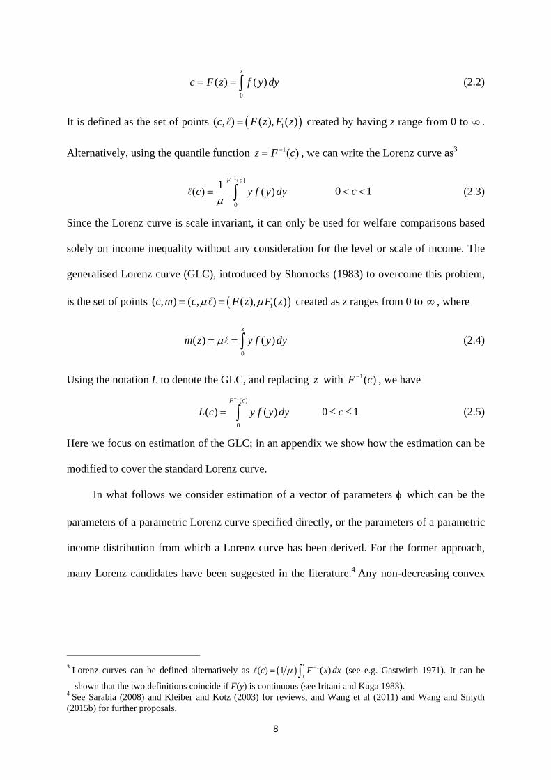
8

0

( ) ( )z

c F z f y dy (2.2)

It is defined as the set of points 1( , ) ( ), ( )c F z F z created by having z range from 0 to .

Alternatively, using the quantile function 1( )z F c , we can write the Lorenz curve as3

1( )

0

1( ) ( )

F c

c y f y dy

0 1c (2.3)

Since the Lorenz curve is scale invariant, it can only be used for welfare comparisons based

solely on income inequality without any consideration for the level or scale of income. The

generalised Lorenz curve (GLC), introduced by Shorrocks (1983) to overcome this problem,

is the set of points 1( , ) ( , ) ( ), ( )c m c F z F z created as z ranges from 0 to , where

0

( ) ( )z

m z y f y dy (2.4)

Using the notation L to denote the GLC, and replacing z with 1( )F c , we have

1( )

0

( ) ( ) 0 1F c

L c y f y dy c

(2.5)

Here we focus on estimation of the GLC; in an appendix we show how the estimation can be

modified to cover the standard Lorenz curve.

In what follows we consider estimation of a vector of parameters which can be the

parameters of a parametric Lorenz curve specified directly, or the parameters of a parametric

income distribution from which a Lorenz curve has been derived. For the former approach,

many Lorenz candidates have been suggested in the literature.4 Any non-decreasing convex

3 Lorenz curves can be defined alternatively as 1

0( ) 1 ( )

cc F x dx (see e.g. Gastwirth 1971). It can be

shown that the two definitions coincide if F(y) is continuous (see Iritani and Kuga 1983). 4 See Sarabia (2008) and Kleiber and Kotz (2003) for reviews, and Wang et al (2011) and Wang and Smyth (2015b) for further proposals.

9

function ( )L c where [0,1]c , (0 ) 0,L and (1 )L , can be a generalised Lorenz curve.5

An example considered later in the paper is the Lorenz curve

31 2( ) 1 (1 )L c c c

(2.6)

This curve was proposed by Sarabia et al. (1999) as a generalisation of the models in Rasche

et al. (1980) and Ortega et al. (1991). Henceforth we refer to it as the SCS curve in line with

the names of its developers. Sufficient conditions for it to satisfy the requirements of a

Lorenz curve are 1 20, 0 , 0 and 3 1 . If our objective is to estimate the Lorenz

curve in (2.6), then 1 2 3, , , .

As an example of Lorenz curve estimation that begins by specifying a parametric

income distribution, consider the generalised beta distribution of the second kind (GB2)

1

( ; )( , )[1 ( ) ]

ap

ap a p q

ayf y

b p q y b

B

(2.7)

with positive parameters , , , )b p q a , and with ( , )p qB denoting the beta function. This

distribution has been a flexible and popular candidate for income distributions (see e.g.,

McDonald 1984, McDonald and Ransom 2008, or Kleiber and Kotz 2003). Its cumulative

distribution function (cdf) is given by

1 1

0

1( ; ) (1 ) ; ,

( , )

up qF y t t dt B u p q

p q B

where a a au y b y , and ( ; , )B u p q is the cdf for the normalised beta distribution defined

on the (0,1) interval. To find the Lorenz curve corresponding to (2.5), we use the following

results (see e.g., Kleiber and Kotz 2003, Ch.6)

( ; , )

; 1 , 1( 1 , 1 )

( , )

b p a q a

p q

c B u p q

m B u p a q a

B

B

(2.8)

5 See, for example, Iritani and Kuga (1983) and Thistle (1989).

10

where, in line with (2.2) and (2.4), a a au z b z . From the first equation in (2.8) we have

1( ; , )u B c p q . Substituting this expression for u into the second equation yields the Lorenz

curve in terms of the parameters of the income distribution

1( ; ) ( ; , )1 , 1

( , ); 1 , 1

b p a q a

p qL c B B c p q p a q a

B

B (2.9)

To provide a statistically sound method of inference for Lorenz curves based on

grouped data, whether it be for a directly specified curve such as (2.6), or an indirectly

specified curve like (2.9), we first need to know how the groupings have been made. The

nature of the groupings defines the DGP, the model, the distribution theory for estimation,

and a choice of suitable notation. As a first step towards some notation that we later modify

slightly according to the DGP, assume that a sample of T observations 1 2, , , Ty y y is

randomly drawn from the income distribution, and placed into N income groups defined by

the group boundaries 0 1( , ),z z 1 2 1( , ), , ( , )N Nz z z z , where 0 0z and Nz . Let iT be the

number of observations and iM total income in the i-th group, and set 11

i

i jjc T T

and

11

i

i jjy T M

. We consider two ways in which the data can be grouped.6

DGP 1: Fixed ic and stochastic iz

Here the observations are grouped such that the proportion of observations in each

group is pre-specified. Examples are 10 groups with 10% of the observations in each group or

20 groups with 5% of the observations in each group. In this case, the cumulative proportions

ic are fixed (non-random) and the sample group boundaries as well as the average cumulative

incomes iy , are random variables. The sample group boundaries are given by

max ( )i t i tz y h y , where ( )i th y is an indicator function equal to one if ty is in the i-th

6 In an unpublished work, Wu (2006) has also distinguished between these two cases and has derived estimators for densities with grouped data. Here, our focus is on Lorenz curves and therefore the resulting moment conditions and weight matrix are different.

11

group and zero otherwise, and where we use a tilde “~” on iz to recognise its randomness.

Define vectors 1 2 1( , , , )Nz z z z and 1 2, , ,L L L LNy y y y . We use the subscript L on Ly

to distinguish it from the average cumulative incomes that we later introduce under DGP 2.

The sample group boundary iz is an estimator for the quantile 1( ; )iF c , and the average

cumulative income Liy is an estimator for the Lorenz ordinate ( ;iL c . If the available

grouped data includes information on z as well as data on 1 2 1= , , , Nc c c c and Ly , then

both z and Ly can be used to estimate . If the sample group boundaries are not available,

one can proceed with estimation based solely on Ly .7

DGP 2: Stochastic ic and fixed iz

The second way in which grouping can take place is with pre-specified group

boundaries in which case 1 2 1( , , , )Nz z z z is predetermined and the cumulative population

shares ic and average cumulative incomes iy are random. An example would be

1 $30,000z , 2 $60,000z , 3 $90,000z , and so on, although equal intervals are not

essential. In this case we use the notation 11

i

i jjc T T

to denote an estimator for ( ; )iF z ,

with 1 2 1, , , Nc c c c . Introducing a subscript m for the cumulative incomes, we have

1 2, , ,m m m mNy y y y where miy is an estimator for ( ;im z . In this case both c and my

can be used to estimate ; if the group boundaries are not provided, then they can be

estimated along with .

These issues are taken up in the next two sections, with DGP 1 being considered in

Section 3 and DGP 2 in Section 4.

7 The possible unavailability of group boundaries is in line with the data on PovcalNet where population and income shares and mean income are provided, from which the ic and iy can be readily calculated; the iz

traditionally have not been provided, but have recently been posted for some countries.

12

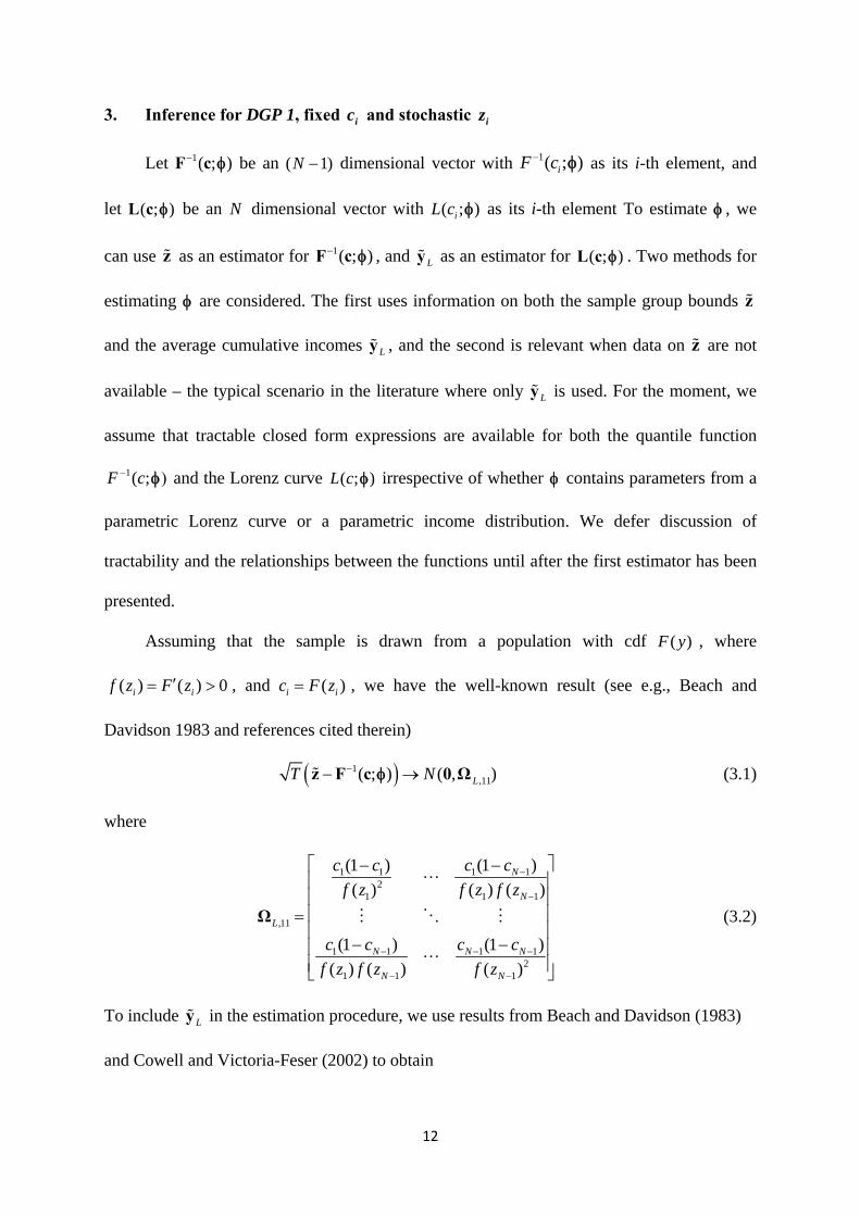
3. Inference for DGP 1, fixed ic and stochastic iz

Let 1( ; )F c be an ( 1)N dimensional vector with 1( ; )iF c as its i-th element, and

let ( ; )L c be an N dimensional vector with ( ; )iL c as its i-th element To estimate , we

can use z as an estimator for 1( ; )F c , and Ly as an estimator for ( ; )L c . Two methods for

estimating are considered. The first uses information on both the sample group bounds z

and the average cumulative incomes Ly , and the second is relevant when data on z are not

available – the typical scenario in the literature where only Ly is used. For the moment, we

assume that tractable closed form expressions are available for both the quantile function

1( ;F c and the Lorenz curve ( ; )L c irrespective of whether contains parameters from a

parametric Lorenz curve or a parametric income distribution. We defer discussion of

tractability and the relationships between the functions until after the first estimator has been

presented.

Assuming that the sample is drawn from a population with cdf ( )F y , where

( ) ( ) 0i if z F z , and ( )i ic F z , we have the well-known result (see e.g., Beach and

Davidson 1983 and references cited therein)

1,11( ; ) ( , )LT N z F c 0 Ω (3.1)

where

1 1 1 12

1 1 1

,11

1 1 1 12

1 1 1

(1 ) (1 )

( ) ( ) ( )

(1 ) (1 )

( ) ( ) ( )

N

N

L

N N N

N N

c c c c

f z f z f z

c c c c

f z f z f z

Ω

(3.2)

To include Ly in the estimation procedure, we use results from Beach and Davidson (1983)

and Cowell and Victoria-Feser (2002) to obtain

13

, 22( ; ) ( , )L LT N y L c 0 Ω (3.3)

where the elements in , 22LΩ are

(2), 22 ,

( ) ( ) ( )L i i i i j j j j i ii jm c z L c z c z L c z L c Ω for i j (3.4)

with

(2) (2) 2

0

( ) ( )iz

i im m z y f y dy (3.5)

Symmetry is used to establish the elements for i j . To combine z and Ly in an estimation

procedure, we also need the asymptotic covariance matrix ,12 cov ,L LT TΩ z y . In

Appendix 1 we show that

,12 ,

,12 ,

for ( ) ( )

( )

( 1) (fo

)

( )r

i j j j j i

L i ji

i j j j

L i ji

ic L c z c z L c

f z

c L c

j

z

zi j

c

f

Ω

Ω

(3.6)

Collecting all these results together, we have

1( ; )( , )

( ; )L

L

T N

z F c0 Ω

y L c

where ,11 ,12

,12 ,22

L L

L

L L

Ω ΩΩ

Ω Ω (3.7)

If we have extra information that can be used to estimate the (2)im , such as group variances,

we can use this information along with iz and ,L iy to consistently estimate ,22LΩ , making it

possible to find standard errors for the Lorenz ordinates ,L iy without making any parametric

assumptions. However, group variances are seldom if ever provided with grouped data. This

problem can be overcome if one is willing to make a parametric assumption about either the

income distribution or the Lorenz curve. Making such an assumption means that (2)im , iz ,

( )if z and ( )iL c can be expressed in terms of the parameters of the income distribution or the

Lorenz curve, and a minimum distance framework can be set up to estimate those parameters.

14

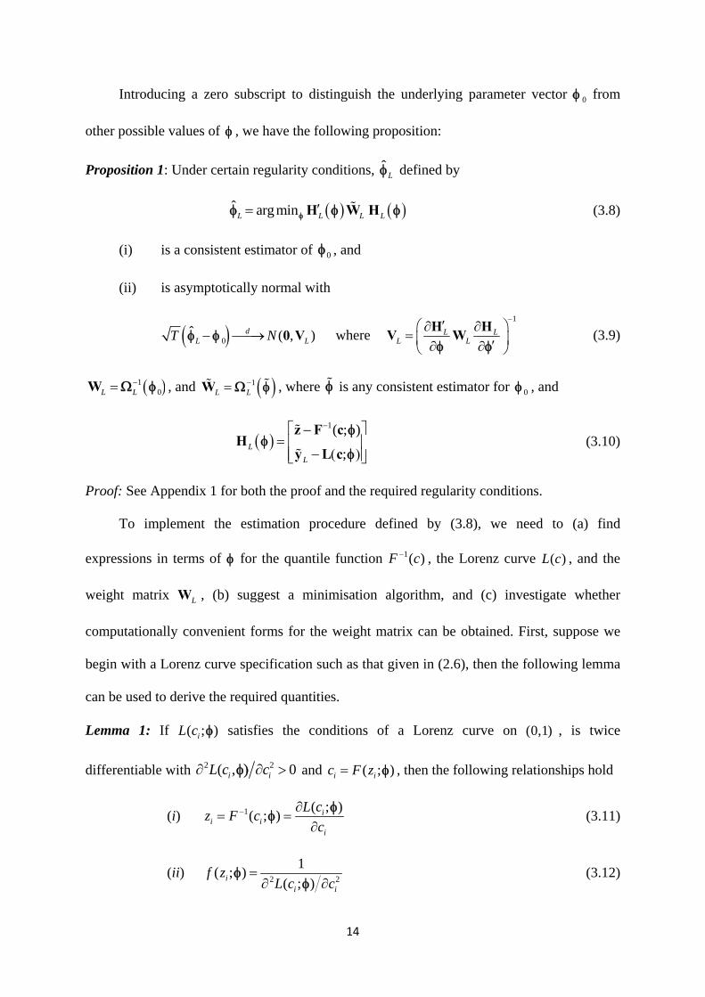
Introducing a zero subscript to distinguish the underlying parameter vector 0 from

other possible values of , we have the following proposition:

Proposition 1: Under certain regularity conditions, ˆL defined by

ˆ arg minL L L L H W H (3.8)

(i) is a consistent estimator of 0 , and

(ii) is asymptotically normal with

0ˆ ( , )dL LT N 0 V where

1

L LL L

H HV W

(3.9)

10L L

W , and 1L L

W , where is any consistent estimator for 0 , and

1( ; )

;L

L

z F cH

y L c

(3.10)

Proof: See Appendix 1 for both the proof and the required regularity conditions.

To implement the estimation procedure defined by (3.8), we need to (a) find

expressions in terms of for the quantile function 1( )F c , the Lorenz curve ( )L c , and the

weight matrix LW , (b) suggest a minimisation algorithm, and (c) investigate whether

computationally convenient forms for the weight matrix can be obtained. First, suppose we

begin with a Lorenz curve specification such as that given in (2.6), then the following lemma

can be used to derive the required quantities.

Lemma 1: If ( ; )iL c satisfies the conditions of a Lorenz curve on (0,1) , is twice

differentiable with 2 2( , 0i iL c c and ( ; )i ic F z , then the following relationships hold

(i) 1 ( ; )( ; ) i

i ii

L cz F c

c

(3.11)

(ii) 2 2

1( ; )

( ; )ii i

f zL c c

(3.12)

15

(iii)

2

(2) 2

0 0

( ; )( ; ) ( ; )

i iz c

ii i i

i

L xm z y f y dy dx

x

(3.13)

Proof: (i) is a well-known result in the Lorenz curve literature (see e.g. Gastwirth 1971), (ii)

is also well-known and can obtained by using (i) and applying the chain rule, and (iii) is

obtained by using (i) and a change of variable for integration.

As an example, applying (i) to the Lorenz curve in (2.6), yields

2

31 2

2

11 1 2 3( ; ) (1 )( ; ) 1 (1 )

1 (1 )i i

i i i ii i i

L c cz F c c c

c c c

(3.14)

From (ii), further differentiation of this function yields an expression for ( ; )if z . A value for

(2) ( ; )i im z can be obtained by numerically integrating the right side of (3.13).

If at the outset we begin by specifying a density function rather than a Lorenz curve,

then whether or not estimation via (3.8) is tractable will depend on whether the cdf is

invertible, either algebraically or computationally. For the GB2 distribution in (2.7), we can

readily derive

11

11

( ; , );

1 ( ; , )

a

i i

B c p qz F c b

B c p q

(3.15)

and the Lorenz curve is given in (3.8), making estimation tractable. In some other cases, such

as a mixture of lognormal distributions, inversion of the cdf is not straightforward, making

estimation difficult computationally. The remaining ingredient needed for estimation of the

GB2 distribution and its Lorenz curve is the quantity (2)im which appears in the weight

matrix. It is given by

(2) (2)2

( 2 , 2 ) ( , )( ) ( ; 2 , 2 )

( 1 , 1 )i i i i

p a q a p qm z m B u p a q a

p a q a

B BB

For a minimisation algorithm one can use any of several methods for implementing

minimum distance estimators including a simple two-step, an iterative two-step or a

16

continuously updating estimator. We employ an iterative two-step estimator where in the first

stage we find 1,1 ,1

ˆ arg minL L L LH Ω H with ,1L I or some other pre-specified

positive definite matrix. Using ,1ˆ

L we compute ,2 ,1ˆ

L L L , then, in the second stage, we

find 1,2 ,2

ˆ arg minL L L L H Ω H . We iterate this process until there is no improvement

in the objective function. Having the estimates, the following equation can be used to

compute the covariance matrix (and standard errors) for ˆL and functions of them such as the

Lorenz curve ordinates or inequality measures

1ˆ ˆ1ˆ ˆvar L L

L LT

H HW

(3.16)

Computationally, it is convenient if we can obtain a closed form solution for the inverse

1L L

W , and simplify computations in other ways, particularly when we have a large

number of groups. In Section 5 we use results from the setup under DGP 2 to derive a closed

form expression for LW . In Appendix 2, we prove the following proposition showing that

most elements in the weight matrix are zeroes.

Proposition 2:

Each block in the weight matrix

1

,11 ,12 ,11 ,12

,12 ,22 ,12 ,22

L L L LL

L L L L

W W Ω ΩW

W W Ω Ωis tri-diagonal.

So far the assumption has been that we have observations on iz . However, there are

many important data sets, for example those provided by the World Bank or WIDER, that do

not report iz ’s. Fortunately, with parametric assumptions we can still estimate by

considering only the second set of equations in (3.10) from which we obtain the estimator

1,0 , 22

ˆ arg min ; ;L L L L y L c Ω y L c (3.17)

17

This method of estimation is the closest to the traditional method of estimation of Lorenz

curves and for this reason we place special emphasis on it. An estimate of its asymptotic

covariance matrix is

1

1,0 ,22

ˆ ˆ1ˆ ˆvar L LT

L LΩ

(3.18)

As one would expect, this estimator is asymptotically less efficient than that in equation (3.8)

where more information is used (see Appendix 1 for a proof). Other characteristics of (3.17)

are that the weight matrix, in this case 1, 22L , is no longer tri-diagonal, and it no longer

depends on ( )if z ; only on (2)im , ic , iz , and ( )iL c .

3.1 Comparison with Conventional Estimation Methods

The estimator in (3.17) provides a context useful for examining most conventional

methods for estimating Lorenz curves. Typically, income shares are regressed against a

Lorenz function of population shares using linear or nonlinear least squares (e.g., Kakwani

1980, Basmann et al 1990, Chotikapanich 1993, Ryu and Slottje 1996, Datt 1998, and the

World Bank website PovcalNet). In general, this estimation problem can be written as

1 2

1

min ( ; )N

i ii

c

(3.19)

where the i are observed income shares, the ic are observed population shares and ( ; )ic

is a parametric Lorenz curve. The generalised Lorenz curve version can be written as8

2

1

min ( ; )N

i ii

y L c

(3.20)

These methods of estimation ignore the fact that observations on cumulative income

proportions are not independent, the consequences of which are inefficient estimates for ,

and incorrect covariance matrices for making inferences about , and quantities that depend

8 In (3.19) does not include whereas it would typically be included in (3.20).

18

on , such as the Gini coefficient9. The estimators from (3.20) and (3.17) are identical if

1,22L

I . Thus, minimising (3.20) yields a consistent estimator for that can be employed

(as we do) to find a first-stage estimate for 1,22L

for use in a repeated two-stage estimation

framework applied to (3.17). However, ignoring the inefficiency that arises from using the

estimates from (3.20) as the end result can make a difference. As is shown in our simulations

and examples in Sections 5 and 6, the diagonal elements in 1,22L

are substantially different

from each other. In (3.17) the weights applied to the initial elements in ;L y L c are much

larger than the weights applied to the later elements, leading to estimates that can be

substantially different from those obtained by minimising (3.20).10

The second issue with conventional least-squares based estimation approaches is that

they have overlooked using the correct covariance matrix for making inferences about . To

obtain this covariance matrix, we note that, from minimum distance estimation theory (see

e.g., Newey-McFadden 1994, theorems 2.1 and 3.2), and for any positive semi-definite

weight matrix Ξ, the estimator

ˆ arg min L L y L c Ξ y L c (3.21)

is consistent and asymptotically normal with covariance matrix estimated by

1 1

,22

ˆ ˆ ˆ ˆ ˆ ˆ1ˆ ˆvar ( )LT

L L L L L LΞ Ξ Ξ Ξ

(3.22)

In the least-squares case where Ξ I , this reduces to

1 1

,22

ˆ ˆ ˆ ˆ ˆ ˆ1ˆ ˆvar ( )LT

L L L L L L

(3.23)

9 Kakwani and Podder (1976) and Chotikapanich and Griffiths (2002) have proposed ways to deal with these facts but their proposals are not built on transparent data generating processes and hence are not fully satisfactory. 10 Our discussion has been in terms of the generalised Lorenz curve. Using the results in Appendix 4, it can be easily modified to be applicable to standard Lorenz curves.

19

This is a more satisfactory covariance matrix than that routinely produced by least squares

estimation.

It is also informative to put the “balanced fit” estimation procedure proposed by Wang

et al (2011) within the context of the minimum distance estimator in (3.8) where information

on both the Lorenz ordinates and the quantile function is used. They recommend minimising

2

1 12

1 1

( ; )( ; ) (1 )

N Ni

i i ii i i

cb c b z

c

where 0 1b is a pre-specified constant. Within our generalised Lorenz curve framework

in (3.8), this approach is equivalent to setting ,11L bW I , ,22 (1 )L b W I and ,12L W 0 . It is

less efficient than using the optimal weight matrix. The relevant covariance matrix for finding

standard errors can be found by adapting (3.22) to the case where both sets of information are

used.11

4. Inference for DGP 2, stochastic ic and fixed iz

Now we turn to the second DGP where the group boundaries z can be viewed as

having been set prior to sampling and the random quantities are the cumulative proportions c

and the average cumulative incomes my . Let ( ; )F z and ( ; )m z be ( 1)N and N-

dimensional vectors, respectively, with i-th elements ( ;iF z and ( ; )im z . Recognising that

c is an estimator for ( ; )F z and my is an estimator for ( ; )m z , we provide the moment

conditions, the optimal weight matrix and a GMM strategy for estimating either ( , ) z ,

or, if the group boundaries are provided, just . Let ( )ig y be an indicator function such that

( ) 1ig y if 0 iy z and ( ) 0ig y otherwise, then the cumulative proportions and the

average cumulative incomes can be written respectively as

11 Wang et al (2011) use bootstrapping to obtain standard errors.

20

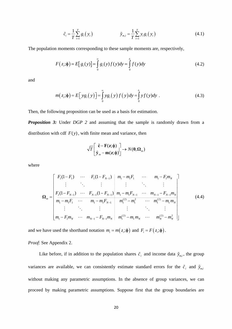
1

1 T

i i tt

c g yT

,1

1 T

m i t i tt

y y g yT

(4.1)

The population moments corresponding to these sample moments are, respectively,

0 0

; ( ) ( ) ( ) ( )iz

i i iF z E g y g y f y dy f y dy

(4.2)

and

0 0

; ( )iz

i i im z E yg y yg y f y dy y f y dy

. (4.3)

Then, the following proposition can be used as a basis for estimation.

Proposition 3: Under DGP 2 and assuming that the sample is randomly drawn from a

distribution with cdf ( )F y , with finite mean and variance, then

( ; )( , )

( ; ) mm

T N

c F z0 Ω

y m z

where

1 1 1 1 1 1 1 1 1

1 1 1 1 1 1 1 1 1

(2) 2 (2)1 1 1 1 1 1 1 1 1 1

(2) (2) 21 1 1 1 1 1

(1 ) (1 )

(1 ) (1 )

N N

N N N N N N N

m

N N

N N N N N N N

F F F F m m F m F m

F F F F m m F m F m

m m F m m F m m m m m

m F m m F m m m m m m

Ω

(4.4)

and we have used the shorthand notation ;i im m z and ;i iF F z .

Proof: See Appendix 2.

Like before, if in addition to the population shares ic and income data ,m iy , the group

variances are available, we can consistently estimate standard errors for the ic and ,m iy

without making any parametric assumptions. In the absence of group variances, we can

proceed by making parametric assumptions. Suppose first that the group boundaries are

21

unknown and are treated as parameters to be estimated. Let the complete set of unknown

parameters be given by 0 0, z .

Proposition 4: Under certain regularity conditions, the GMM estimator θ given by

ˆ arg min m m m θθ H θ W H θ (4.5)

(i) is a consistent estimator of 0 , and

(ii) is asymptotically normal with

0ˆ ( , )d

mT N θ θ 0 V where 1

m mm m

H H

V Wθ θ

(4.6)

m

m

c F θH θ

y m θ

(4.7)

10( )m m

W Ω θ , 1( )m mW Ω θ where θ is any consistent estimator for 0θ , and mΩ is the

covariance matrix of the limiting distribution of mT H from (4.4).

Proof: See Appendix 2 for the proof and the regularity conditions.

If the starting point is specification of a parametric income distribution, then the

estimator in (4.5) will be tractable providing we have a satisfactory way for computing values

of its cdf and its first and 2nd moment distribution functions. That is, iF , im and (2)im can be

readily calculated. Such is the case for the GB2 distribution, for example. Whether or not

estimation is tractable when the starting point is a parametric Lorenz curve will depend on

whether the cdf can be obtained by inverting the quantile function. The quantile function

given in (3.14) for the Sarabia GLC cannot be readily inverted such that ic is written as a

function of iz , making estimation intractable for this case. More light will be shed on this

issue with further examples in Section 6.

Again, an iterative two-step GMM estimator works well in practice. In the first stage,

we set 2 2 2 2,1 1 ,1 , Diag( , , , , , )m N m m Nc c y y Ω and find 1

1 ,1ˆ arg min m m m

θθ H θ Ω H θ . In the

22

second stage we find 12 1

ˆ ˆargmin m m m θθ H θ Ω θ H θ , and then we iterate until

convergence. The rationale behind using ,1mΩ in the first step is that it leads to an estimator

that minimizes the sum of squares of the percentage errors in the moment conditions. After

estimation, (4.6) can be used to compute standard errors for the elements in and functions

of them. Note also that when the iz ’s are known, the same procedure can be followed, the

only difference is that the number of parameters to be estimated is less.

Computations can be simplified by recognising that the 4 blocks in the weight matrix

mW are tri-diagonal. Commensurate with the partitioning of mH θ in (4.7), let mW be

partitioned as

,11 ,12

,12 ,22

m m

m

m m

W WW

W W

Proposition 5: Let 1( ; ) ( ; )i i i iF z F z θ , 1( ; ) ( ; )i i i im z m z θ ,

(2) (2) (2) (2)1( ; ) ( ; )i i i im z m z θ , and (2) 2

i i i iv . Each of the blocks ,m ijW is tri-

diagonal, with the following elements

23

Proof: See Appendix 2.

5. Some Relationships Between DGP 1 and DGP 2

In terms of implementation, two advantages of DGP 2 are that we have a closed form

expression for the weight matrix and we have access to a richer collection of functions with

good properties [e.g., generalised beta, mixture of lognormals, etc.] to choose from. However,

the model developed for DGP 1 is more in line with traditional Lorenz curve estimation and,

in the absence of information on the class bounds, it can work with only estimating the

second (i.e., “mean”) set of equations that uses information on Ly . In this Section we give

expressions for the relationship between the weight matrices for the two estimation

procedures, expressions that can be utilised to compute the weight matrices for estimation

under DGP 1 from the weight matrix under DGP 2. Let from DGP 2 be partitioned as

ˆ ˆˆ , m z . We also show, under “equivalent conditions” stated in Proposition 6, that the

asymptotic variances for the two estimators ˆL and ˆ

m are the same.

In what follows, we use the following notation: if 1, , na a a and 1, , nb b b ,

then 1 1, , n na b a b a.b , 1 1 , , n na b a b a b , and [ ]D a is a diagonal matrix with the

elements of a on the diagonal. Also, we use (1, ,1) j to denote a vector of ones.

24

Proposition 6: Suppose group bounds z in DGP 2 and population shares c in DGP 1 are

chosen in a way that 1( )z F c then12

(i) =L m Ω AΩ A with 1 ( 1)

1

1 ( 1)

[ ( )]

[ ]N N N

N

NN

D

D

j f z 0

zAI

0

- - ´

-

´ -

æ ö- ÷ç ÷ç ÷ç ÷é ù-=ç ÷ç ê ú ÷ç ÷ê úç ÷÷çè øë û

(ii) 1 1L m

W A W A with 1 ( 1)

11

1 ( 1)

[ ( )]

[ ( ). ]N N N

N

NN

D

D

f z 0

f z zAI

0

- - ´

--

´ -

æ ö- ÷ç ÷ç ÷ç ÷é ù-=ç ÷çê ú ÷ç ÷ê úç ÷÷çè øë û

and the lower diagonal blocks of LW and mW are equal.

(iii) 1 1 1 1 1,22 ( ) ( ) [ ( ) ] ( )L m m m m m

Ω BΩ B BB B W W C C W C C W B BB

with 1

1 ( 1)

[ ]N

NN

D zB I

0-

´ -

æ öé ù- ÷çê ú ÷ç= ÷çê ú ÷÷çè øë û and 1 1 ( 1) 1[ [ ] ]N N ND C I z 0

Proof: (i) can be shown by direct multiplication after recognising that ( )i ic F z and that this

implies ( ) ( )i im z L c . To prove (ii) note that 11 1 1L L m m

W Ω AΩ A A W A . The

particular form of 1A- can be checked by showing that 1AA I- = . The equality of the lower

diagonal blocks of LW and mW can be checked by multiplication. The first equality in (iii)

comes from (i). To prove the second equality in (iii), we first note that

1 1( ) ( ) B BB B I C C C C

from which it follows that

1 1 1[ ( ) ] ( ) [ ( ) ]m m m m I C C W C C W B BB B I C C W C C W

Then, postmultiplying the right hand side of (iii) by m BΩ B yields

12 The result in (i) might also be of interest to distribution free studies since the lower diagonal block provides the relationship between the variances of the Lorenz ordinates under the two DGPs, Ly and my .

25

1 1 1

1 1

1 1

1

( ) [ ( ) ] ( ) [ ]

( ) [ ( ) ]

( ) [ ( ) ] since

( ) since

m m m m

m m m m

m m m m m

BB BW I C C W C C W B BB BΩ B

BB BW I C C W C C W Ω B

BB BW Ω B C C W C C B W Ω I

BB BB C B 0

I

Result (ii) in this proposition provides a closed form for the weight matrix for DGP 1

when both quantile and Lorenz equations are considered. The result in (iii) provides a

tractable formula for the weight matrix when only the Lorenz equations are considered (see

equation (3.17)). Its tractability comes from the facts that BB is diagonal, mC W C is tri-

diagonal and there are special formulae for inverting such matrices.

It can also be shown that the two methods provide the same asymptotic variance for

if the a priori groupings from both methods are equivalent. For example, if data are grouped

under DGP 1 into say 10 equal groups with (0.1,...,0.9)c and under DGP 2 the bounds are

specified as 0 0[ (0.1, ),...., (0.9, )]F F z , then the asymptotic variances of the estimated

parameters from the two cases are equal13. More formally:

Proposition-7

(i) Known group bounds: If 10( )i iz F c , then the asymptotic variance of ˆ

L

under DGP 1 with observed , , , i L i ic y z is equal to asymptotic variance of ˆm

under DGP 2 with observed , , , i m i ic y z . That is,

1 1111 1( ) ( )L mT T

FFF L F mW W

mL

where both are evaluated at 0 .

13 Note that, after sampling, the resulting grouped data will be different in the two cases even if the grouping is made on the same random sample.

26

(ii) Unobserved group bounds: The asymptotic variance of ˆL under DGP 1 with

observed , i ic y is equal to the asymptotic variance of ˆm under DGP 2 with

observed , i ic y . That is, 1

1,22

1( )LT

L LΩ

evaluated at 0 is equal to the

lower diagonal block of 1

1ˆcov ( )mT

F θF mθ W θ

m θθ θ evaluated

at 10 0 0[ ( , ) , ] θ F c .

Proof : See Appendix 3.

To prove the above proposition we need the following lemma which might be of

interest on its own.

Lemma 2: If ( ; )i ic F z , then under suitable differentiability conditions, we have the

following results:

(i) 11 1 2 2

2

( ; ) ( ; )( ; ) ( ; ) ( ; ) ( ; )( )i ii i i i

ij i i j ij j

F z F cF c F c L c L cf z

c c c

(ii) 2

2 2

( ; )( ; ) ( ; ) ( ; )

( ; )i i ji i i

j j i i i

L c cm z L c L c

c L c c

(iii) ( ; ) ( ; ) ( ; )i i i

ij j j

L c m z F zz

Proof : (i) can be obtained by differentiating 1( ; );i iF F c c with respect to j , applying

the chain rule and the results from Lemma 1; (ii) is obtained by differentiating

( ) ( , );i im z L F z with respect to j , applying the chain rule and the result from (i);

and (iii) is obtained by differentiating 1( ; ) ( ; );i iL c m F c with respect to j , applying

the chain rule and the result from (i).

27

6. Monte Carlo Experiment

Here we perform a Monte Carlo experiment to address the following questions: (i) Do

the estimators perform well? (ii) Does the method of grouping matter? (iii) How do the

various estimators compare with each other and with some traditional Lorenz curve

estimation methods? (iv) How do the estimators perform in finite samples?

With the exception of one experiment, the data for all simulations were obtained by

drawing 10,000 observations from a GB2 distribution with 100b , 1p , 1.5q and

1.5a , implying a relatively heavy-tailed Singh-Maddala distribution with a Gini coefficient

of 0.53.14 A heavy-tailed case was considered because inference in such cases can be more

challenging. Although the data were generated from the Singh-Maddala distribution, the

more general GB2 distribution was estimated.

In the first experiment we investigate the performance of covariance matrix estimators

for the Lorenz ordinates without making any distributional assumptions. The generated

10,000 observations were used to create 5 groups based on the two grouping methods. For

DGP 1, the data were grouped by dividing the simulated sample into 5 equally-sized groups

with (0.2,0.4, ,0.8) c ; then the associated iy s and iz s were computed. For DGP 2, the

groups bounds ( 's)iz were set according to the theoretical quantiles corresponding to c , and

the associated iy and ic were computed. We restricted the number of groups to 5 in this case

for ease of presentation of the results. For later experiments we used 20 groups with

corresponding cumulative proportions (0.05,0.1, ,0.95) c . The two covariance matrices

being considered are ,22L and ,22m given in (3.4) and (4.4), respectively. In (3.4), ,L iy is

used to estimate ( )iL c ; when the grouping is made, we also compute (2) 1 2, 1

( )T

L i t i tty T y g y

14 A Singh-Maddala distribution is a special case of the GB2 where 1p . A necessary and sufficient condition

for the existence of the k-th moment of the GB2 is aq k . Thus, for 1.5a q , moments beyond the second

one do not exist.

28

which is used to estimate (2)im . In (4.4), ,m iy is used to estimate im and (2)

,m iy is used to

estimate (2)im .

Table 1 contains the results from 500 replications. Its first panel provides the Monte

Carlo averages of the estimates for ,22L and ,22m . The second panel contains the Monte

Carlo covariance matrix of the simulated Lorenz ordinates. The matrices ,22L and ,22m

evaluated at the true values of the parameters appear in the 3rd panel, and the inverses of these

matrices are in the final panel. The values in the first three panels for each of the DGPs are

largely similar confirming the validity of the formulae. There are somewhat large differences

between alternative variances of the last group mean where 5y is an estimate of the mean .

This appears to be attributable to the heavy-tailed distribution which is close to having an

infinite second order moment. The differences are reduced when the number of Monte Carlo

replications is increased and substantially reduced if the data are generated from a

distribution with a narrower tail. A comparison of the DGP 1 and DGP 2 covariance matrices

shows that their variances can be substantially different. The variances for the initial groups

are smaller for DGP 1, they become larger for the later groups and become equal as expected

for the last group where in both cases the mean is being estimated. These results are evident

from the formula

DGP 1: (2) 2,22 (1 )( 2 )L i i i i i i iii

m m z c c z m

DGP 2: (2) 2,22m i iii

m m

As long as 2i i ic z m (which happens for the initial groups with typical income distributions)

the DGP 1 variance is smaller. Also the variances are equal when 1ic . We can also see

(both theoretically and from the simulation) that the covariances from DGP 1 are always

positive but for DGP 2 they could be positive or negative. Finally, the inverses of the

covariance matrices, i.e., the weight matrices for both DGPs, are starkly different from the

identity matrix which is often used implicitly in least square estimation.

29

Table-1: Covariance matrix for iy s using a distribution free approach

Covariance Matrix of Lorenz Ordinates DGP 1 Covariance Matrix of Lorenz Ordinates DGP 2

Formula (3.4) at Sample Information Formula (4.4) at Sample Information

1y 2y 3y 4y 5y 1y 2y 3y 4y 5y

1y 0.377 0.822 1.249 1.722 2.598 0.578 0.296 ‐0.182 ‐0.973 ‐3.193

2y 0.822 2.405 4.130 6.037 9.573 0.296 2.912 1.253 ‐1.496 ‐9.203

3y 1.249 4.130 8.419 13.589 23.179 ‐0.182 1.253 7.793 1.731 ‐15.267

4y 1.722 6.037 13.589 26.117 51.969 ‐0.973 ‐1.496 1.731 18.314 ‐14.072

5y 2.60 9.57 23.18 51.97 512.75 ‐3.19 ‐9.20 ‐15.27 ‐14.07 512.75

Covariance of Simulated Draws Covariance of Simulated Draws

1y 0.382 0.821 1.248 1.691 2.252 0.597 0.293 ‐0.181 ‐1.009 ‐3.192

2y 0.821 2.349 3.993 5.766 8.828 0.293 2.889 1.091 ‐1.589 ‐8.402

3y 1.248 3.993 8.011 12.813 20.382 ‐0.181 1.091 7.862 2.035 ‐11.435

4y 1.691 5.766 12.813 24.883 45.378 ‐1.009 ‐1.589 2.035 18.514 ‐12.559

5y 2.25 8.83 20.38 45.38 444.39 ‐3.19 ‐8.40 ‐11.44 ‐12.56 444.39

Formula (3.4) Computed at True Values Formula (4.4) Computed at True Values

1y 0.377 0.823 1.251 1.724 2.601 0.578 0.296 ‐0.182 ‐0.973 ‐3.191

2y 0.823 2.404 4.129 6.034 9.572 0.296 2.914 1.253 ‐1.497 ‐9.203

3y 1.251 4.129 8.413 13.578 23.168 ‐0.182 1.253 7.795 1.730 ‐15.268

4y 1.724 6.034 13.578 26.089 51.938 ‐0.973 ‐1.497 1.730 18.317 ‐14.068

5y 2.60 9.57 23.17 51.94 615.62 ‐3.19 ‐9.20 ‐15.27 ‐14.07 615.62

Weight Matrix Computed at True Values Weight Matrix Computed at True Values

1y 1335.50 ‐777.03 220.01 ‐23.24 0.119 207.01 ‐15.09 7.51 10.03 1.26

2y ‐777.030 806.520 ‐389.100 67.989 ‐0.349 ‐15.091 42.225 ‐7.051 3.669 0.462

3y 220.010 ‐389.100 304.510 ‐84.608 0.798 7.513 ‐7.051 14.979 ‐1.382 0.273

4y ‐23.244 67.989 ‐84.608 35.151 ‐0.740 10.029 3.669 ‐1.382 6.594 0.223

5y 0.119 ‐0.349 0.798 ‐0.740 0.200 1.263 0.462 0.273 0.223 0.188

In the second experiment we consider estimation of the parameters of the GB2

distribution under DGP 1 using two scenarios: observations on ,, ,i L i ic y z and observations

on ,,i L ic y only. Experimental results from using the minimum distance estimators (3.8) and

(3.17) are given in Table 2. Again, 500 Monte Carlo iterations are used.15 In addition to the

15 In all cases, we conducted repeated minimum distance estimation starting with an identity weight matrix and repeating the process 10 times as explained in Section 3. All estimations were done using code written in MATLAB R2013.

30

GB2 parameters, we also include the Gini coefficient as one of the main quantities of interest

in income distribution studies. The left and right panels in the Table display the results for

observed and unobserved iz , respectively. In each case, the first column provides the average

of the estimated parameters over the Monte-Carlo replications. As it can be seen, they are

almost identical to the true values, suggesting unbiasedness. The second, third and fourth

columns contain, respectively, (i) the asymptotic variances computed at the true parameter

values, (ii) the average of the estimated variances over the replications, and (iii) the Monte

Carlo sample variance of the estimated parameters. There are only minor differences between

the three sets of variances. The sample variances are slightly larger than their asymptotic

counterparts, indicating that there could be some underestimation of the finite sample

variation, but, because the differences are not large, overall we can conclude that the

estimators perform well in finite samples. We also see that estimation with observed iz ’s is

more efficient than estimation with unobserved iz ’s, but the differences are negligible. At

least under the ideal conditions of the Monte Carlo experiment, not knowing the iz ’s has little

impact.

Table-2: Monte Carlo Experiment Results for DGP 1

With data on z With unknown z

True

Par Average Est‐Par

True

Var Average Est‐Var

Variance Est‐Par

Average Est‐Par

True

Var Average Est‐Var

Variance Est‐Par

b 100.00 100.70 32.84 34.68 36.20 100.56 34.06 36.50 37.52

p 1.0000 1.0177 0.0122 0.0123 0.0133 1.0155 0.0125 0.0129 0.0136

q 1.5000 1.5338 0.0417 0.0416 0.0464 1.5290 0.0431 0.0440 0.0479

a 1.5000 1.4941 0.0142 0.0133 0.0145 1.4972 0.0145 0.0140 0.0151

Gini 0.5326 0.5326 0.0071 0.0067 0.0072 0.5328 0.0073 0.0071 0.0074

Our third experiment is again concerned with estimation of the GB2 parameters and the

related Gini coefficient, but this time under DGP 2, using the GMM estimator in (4.5), with

and without the iz treated as unknown parameters. The results appear in Table 3 which

follows the same format as Table 2 except that, for the unknown iz case, we report a

31

selection of estimates of the iz . Our conclusions are similar to those from DGP 1. There is no

evidence that the estimators are biased. The three variances are very similar, with the

asymptotic variance and the average of its estimates slightly understating the Monte-Carlo

estimated variance. Having to estimate the group boundaries reduces efficiency, but not by

much. Comparing the results from DGP 1 and DGP 2, we see that, despite substantial

differences between the models and between the variances of the Lorenz ordinates, the “true”

variances for the parameters are identical as predicted by Proposition 7.

Table-3: Monte Carlo Experiment Results for DGP 2

Known z Unknown z

True

Par Average Est‐Par

True

Var Average Est‐Var

Variance Est‐Par

Average Est‐Par

True

Var Average Est‐Var

Variance Est‐Par

1z 10.656 10.654 0.0159 0.0151 0.0159

2z 17.430 17.438 0.0118 0.0121 0.0118

10z 70.139 70.153 0.0205 0.0208 0.0205

18z 236.70 236.69 1.36 1.63 1.36

19z 343.56 343.65 11.39 10.47 11.50

b 100.00 100.57 32.84 34.78 35.88 100.55 34.06 36.05 37.33

p 1.0000 1.0144 0.0122 0.0123 0.0132 1.0140 0.0125 0.0128 0.0136

q 1.5000 1.5276 0.0417 0.0418 0.0460 1.5268 0.0431 0.0434 0.0477

a 1.5000 1.4976 0.0142 0.0136 0.0146 1.4985 0.0145 0.0140 0.0151

Gini 0.5326 0.5328 0.0071 0.0068 0.0072 0.5328 0.0073 0.0071 0.0075

Our final experiment is designed to compare the performance of the minimum distance

estimator in (3.17) with the least squares estimator in (3.20). Using data generated from DGP

1, and with unknown group bounds, two scenarios are considered. In the first scenario the

data are generated from the GB2 distribution as in the previous experiments, and the

parameters of the distribution are estimated using the Lorenz curve specification in (2.8). In

the second scenario the data are generated consistently with the SCS Lorenz curve

specification in (2.5), and the minimum distance and least squares estimators are used to

32

estimate its parameters.16 As with the GB2 distribution, 10,000 observations were generated

and grouped into 20 groups of equal size. The SCS model parameters 40 , ,

, and 3 3.4 were chosen as close to the estimates from a real data example in

Section 7. They preserve the required properties of a Lorenz curve despite the fact that

violates the sufficient condition that all parameters are positive. The support of the

distribution is [0, ) and the second order moment becomes infinite if 2 0.5 . The results

are presented in Table 4 in the same format as those from the earlier experiments. For the

least squares variances, we use the “correct” formula in (3.23). The minimum distance

estimator has smaller variances in both cases, with the difference being particularly marked

for the GB2 distribution. Also, for least squares applied to the GB2 distribution we see some

relatively large differences between the true variances, the average of the estimated variances,

and the variance of the estimated parameters. These differences can be attributed to the heavy

tail of the assumed distribution since some of the least squares estimates approach values that

yield an infinite second moment.17

There are other questions of interest that can be investigated with Monte Carlo

experiments, such as the effect of the number of groups and the effect of the number of

observations. We address the effect of the number of groups in Section 8. A Monte Carlo

experiment was conducted to examine the effect of increasing the number of observations,

yielding results that were consistent with asymptotic theory. The 10000 observations used for

the results that we have reported is less than the number from most household surveys.

16 To generate the data according to this Lorenz curve, we use the inverse-cdf method and equation (3.14). 17 In fact we have discarded 15 of the Monte Carlo draws in reporting the results for LS-GB2 because of their unreasonably large variances.

1 2

2 0.8

1 2

33

Table-4: Monte Carlo Results, Minimum Distance vs Least Squares

MD‐GB2 LS‐GB2

True

Par Average Est‐Par

True

Var Average Est‐Var

Variance Est‐Par

Average Est‐Par

True

Var Average Est‐Var

Variance Est‐Par

b 100.00 100.56 34.06 36.50 37.52 101.37 39.25 31.14 46.85

p 1.00 1.0155 0.0125 0.0129 0.0136 1.0610 0.0438 0.0353 0.0569

q 1.50 1.5290 0.0431 0.0440 0.0479 1.5984 0.1128 0.0756 0.1422

a 1.50 1.4972 0.0145 0.0140 0.0151 1.4678 0.0432 0.0254 0.0521

Gini 0.5326 0.5328 0.0073 0.0071 0.0074 0.5326 0.0088 0.0070 0.0074

MD‐SCS LS‐SCS

True

Par Average Est‐Par

True

Var Average Est‐Var

Variance Est‐Par

Average Est‐Par

True

Var Average Est‐Var

Variance Est‐Par

40.00 39.98 0.14 0.15 0.14 39.98 0.14 0.15 0.14

1 ‐2.00 ‐2.0924 0.2581 0.2977 0.3065 ‐2.0922 0.3062 0.3384 0.3677

2 0.800 0.8014 0.0006 0.0006 0.0006 0.8010 0.0007 0.0007 0.0007

3 3.40 3.4922 0.2533 0.2917 0.3014 3.4921 0.2983 0.3297 0.3594

Gini 0.4201 0.4199 0.0035 0.0036 0.0035 0.4199 0.0035 0.0036 0.0035

7. World Bank Estimation of Lorenz Curves

The World Bank collects and publishes grouped income or expenditure data for a large

number of countries over time. These data are usually in the form of population and income

shares for a number of groups, typically between 10 and 20. The World Bank website

PovcalNet uses these data to estimates Lorenz curves and, based on these estimates, provides

a variety of poverty and inequality measures.18 The Lorenz specifications that it uses are the

general quadratic (GQ) proposed by Villasenor and Arnold (1989) and the beta proposed by

Kakwani (1980).19 On PovcalNet both of these curves are estimated and the one with the

better fit is chosen to compute poverty and inequality measures.20 In what follows, we first

review the GQ and the beta Lorenz curves and then estimate these models for several 18 Recently, the World Bank has started to publish data in the form of 100 groups and to base inequality and poverty estimates on these groups. Earlier groups and their Lorenz curve estimations are still present on the PovcalNet website, however. 19 The literature abounds with proposals for parametric Lorenz curves. Examples are Kakwani and Podder (1973,1976), Rasche et al. (1980), Gupta (1984), Arnold (1987), Basmann et al. (1990), Chotikapanich (1993), Ryu and Slottje (1996), Sarabia et al. (1999) and Wang et al (2011). The literature is surveyed by Sarabia (2008). 20 See Datt(1998) for details of the World Bank approach.

34

countries, comparing the results from the method employed by PovcalNet with those from

our optimal estimation methods. The results are also compared with those from our preferred

Lorenz curve specifications: GB2 and SCS.

The general quadratic Lorenz curve depends on three parameters 1 2 3, , and can be

written as

21 2 3(1 ) ( ) ( 1) ( )i i i i i i i ic c c (7.1)

The parameters are often estimated by replacing i with the observed cumulative income

proportions and applying least squares to equation (7.1). This practice is not innocuous,

however, since the i s are present on both sides of the equation. To put (7.1) in the

generalised Lorenz framework that we have been using, we let denote the mean of the

distribution and define the following

21 2 3 2 1 2 31 , 4 , 2 4e m n e (7.2)

The GQ generalised Lorenz curve can then be written as

2 22( )

2i i i i iy L c c e mc nc e (7.3)

This can be estimated by applying nonlinear least squares which is not prone to the above

endogeneity problem, but it is still not optimal.21 The optimal minimum distance estimator

can be applied after using Lemma 1 to find the elements required for the weight matrix,

namely, 1( )i iz F c and (2)im .

One problem with beginning a study with specification of a parametric Lorenz curve

rather than a parametric income distribution is that the income distribution implied by the

Lorenz curve may only be valid for a limited range of incomes. Having a finite support for

income can be a serious drawback with potentially important implications since, in poverty 21 Because 2 appears in (7.3), this equation is not a complete reparameterisation of (7.1). When estimating this

Lorenz curve, we minimize the relevant objective function with respect to 1 2, and 3 ; the expressions in

(7.2) are convenient for intermediate calculations.

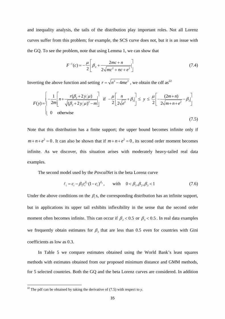
35

and inequality analysis, the tails of the distribution play important roles. Not all Lorenz

curves suffer from this problem; for example, the SCS curve does not, but it is an issue with

the GQ. To see the problem, note that using Lemma 1, we can show that

12 2 2

2( )

2 2

mc nF c

mc nc e

(7.4)

Inverting the above function and setting 2 24r n me , we obtain the cdf as22

22 22 2 2

2

1 ( 2 ) (2 )if

2 2 2( ) ( 2 ) 2 2

0 otherwise

r y n m nn y

mF y y m e m n e

(7.5)

Note that this distribution has a finite support; the upper bound becomes infinite only if

2 0m n e . It can also be shown that if 2 0m n e , its second order moment becomes

infinite. As we discover, this situation arises with moderately heavy-tailed real data

examples.

The second model used by the PovcalNet is the beta Lorenz curve

321 (1 )i i i ic c c , with 1 2 30 , , 1 (7.6)

Under the above conditions on the i s, the corresponding distribution has an infinite support,

but in applications its upper tail exhibits inflexibility in the sense that the second order

moment often becomes infinite. This can occur if 2 0.5 or 3 0.5 . In real data examples

we frequently obtain estimates for 3 that are less than 0.5 even for countries with Gini

coefficients as low as 0.3.

In Table 5 we compare estimates obtained using the World Bank’s least squares

methods with estimates obtained from our proposed minimum distance and GMM methods,

for 5 selected countries. Both the GQ and the beta Lorenz curves are considered. In addition

22 The pdf can be obtained by taking the derivative of (7.5) with respect to y.

36

to the parameter estimates and their standard errors, estimates for the Gini coefficient and the

headcount ratio H (using a poverty line of $38/month) are reported. We also include

estimates obtained using the GB2 and SCS specifications. Useful diagnostic information that

is provided is the supports of the distributions min max[ , ]y y , the J-statistics for testing the

validity of the estimating equations, and the percentage errors in predictions of the incomes

of the first and last groups, 1S and 20S . The data are from 2004 or 2005, extracted from the

PovcalNet website where we obtained population and income shares for 20 groups and mean

income for each country. In all cases the iz s are not observed, DGP 1 is assumed, and

therefore only the second set of equations in (3.10) is considered. The following

abbreviations for the estimators are used in the Table:

(i) OLS-GQ: Least squares estimation applied to (7.1) – the World Bank approach.

(ii) MD-GQ: Minimum distance estimation applied to (7.3).

(iii) NLS-Beta: Nonlinear least squares applied to the generalised Lorenz version of (7.6).

(iv) MD-Beta: Minimum distance estimation applied to the Lorenz curve in (iii).

(v) MD-GB2: Minimum distance estimation applied to the Lorenz curve in (2.9).

(vi) MD-SCS: Minimum distance estimation applied to the Lorenz curve in (2.6).

37

Table 5: A comparison of Lorenz curve estimation methods for selected countries using 2004 or 2005 data.

China Urban

OLS‐GQ MD‐GQ NLS‐Beta MD‐Beta MD‐GB2 MD‐SCS

Par SE Par SE Par Par SE Par SE Par SE

1 b 0.889 0.003 0.912 0.009 0.638 0.641 0.005 108.14 4.857 ‐0.320 0.192

2 p ‐1.260 0.010 ‐1.344 0.018 0.935 0.935 0.003 2.369 0.391 0.708 0.027

3 q 0.187 0.006 0.140 0.005 0.522 0.515 0.011 1.778 0.252 1.621 0.189

a NA NA 160.95 1.216 161.87 162.53 1.426 1.842 0.168 161.47 1.316

Gini 0.347 0.000 0.349 0.004 0.353 0.352 0.004 0.345 0.004 0.347 0.004

H 0.004 NA 0.021 0.001 0.018 0.017 0.001 0.019 0.001 0.021 0.001

miny 36.86 31.80 0 0 0 0

maxy 1487.7 1935.4 J-Stat 278.58 85.124 28.79 28.40 31.079 53.69

S1 ‐6.609 2.152 0.631 ‐0.214 0.497 ‐3.039

S20 ‐0.005 ‐0.546 0.024 0.380 ‐0.418 ‐0.222

Nigeria

OLS‐GQ MD‐GQ NLS‐Beta MD‐Beta MD‐GB2 MD‐SCS

Par SE Par SE Par Par SE Par SE Par SE

1 b 0.979 0.003 0.999 0.010 0.775 0.761 0.005 32.82 3.276 ‐2.001 0.531

2 p ‐0.932 0.015 ‐1.068 0.026 0.974 0.960 0.002 4.88 1.508 0.812 0.025

3 q 0.189 0.006 0.130 0.005 0.538 0.507 0.011 5.202 1.616 3.384 0.527

a NA NA 39.764 0.329 40.272 40.946 0.436 0.893 0.150 40.003 0.353

Gini 0.400 0.000 0.401 0.003 0.404 0.414 0.005 0.401 0.004 0.401 0.003

H 0.619 NA 0.618 0.004 0.614 0.615 0.004 0.620 0.004 0.626 0.004

miny 6.088 4.884 0 0 0 0

maxy 287.37 326.87 J-Stat 399.54 95.164 47.70 NA 39.054 66.779

S1 ‐12.108 2.439 14.408 0.1015 0.099 ‐4.117

S20 ‐0.006 ‐0.640 0.077 2.818 ‐0.090 ‐0.0436

Pakistan

OLS‐GQ MD‐GQ NLS‐Beta MD‐Beta MD‐GB2 MD‐SCS

Par SE Par SE Par Par SE Par SE Par SE

1 b 0.752 0.010 0.853 0.009 0.549 0.538 0.005 39.087 1.140 0.002 0.123

2 p ‐1.267 0.029 ‐1.458 0.015 0.941 0.918 0.003 1.565 0.206 0.641 0.029

3 q 0.269 0.018 0.167 0.005 0.462 0.399 0.014 0.691 0.067 1.186 0.121

a NA NA 63.760 0.465 66.321 68.493 0.818 3.720 0.276 65.734 0.555

Gini 0.312 0.001 0.304 0.004 0.317 0.339 0.007 0.315 0.004 0.311 0.005

H 0.232 NA 0.235 0.004 0.229 0.219 0.004 0.221 0.004 0.216 0.004

miny 22.77 18.932 0 0 0 0

maxy 1569.1 1374.2 J-Stat 4067.9 370.41 NA NA 20.221 15.58

S1 ‐15.207 3.101 8.414 ‐0.309 ‐0.200 0.2099

S20 0.004 ‐3.041 0.061 4.236 0.511 ‐0.039

38

Kenya

OLS‐GQ MD‐GQ NLS‐Beta MD‐Beta MD‐GB2 MD‐SCS

Par SE Par SE Par Par SE Par SE Par SE

1 b 0.755 0.008

Infinite second order moment No estimates are

reported

0.800 0.779 0.005 35.521 1.239 ‐0.038 0.178

2 p ‐0.485 0.048 0.975 0.953 0.002 1.337 0.180 0.544 0.042

3 q 0.222 0.016 0.392 0.322 0.015 1.015 0.133 1.433 0.173

a NA NA 66.949 72.019 1.773 1.967 0.172 65.592 1.287

Gini 0.456 0.010 0.488 0.523 0.011 0.482 0.009 0.477 0.009

H 0.438 NA 0.441 0.438 0.004 0.440 0.004 0.439 0.004

miny 29.188 0 0 0 0

maxy 10615

J-Stat NA NA NA 86.582 81.287

S1 39.686 31.272 ‐0.248 0.985 1.969

S20 ‐0.002 0.055 8.701 1.091 0.186

Iran

OLS‐GQ MD‐GQ NLS‐Beta MD‐Beta MD‐GB2 MS‐SCS

Par SE Par SE Par Par SE Par SE Par SE

1 b 0.888 0.004 0.922 0.010 0.709 0.698 0.005 118.99 7.847 ‐0.822 0.263

2 p ‐1.030 0.018 ‐1.190 0.022 0.957 0.946 0.003 3.059 0.602 0.734 0.026

3 q 0.212 0.008 0.135 0.005 0.504 0.484 0.012 2.258 0.377 2.147 0.260

a NA NA 195.99 1.682 199.09 200.93 2.143 1.426 0.149 197.20 1.781

Gini 0.383 0.000 0.385 0.004 0.388 0.393 0.005 0.383 0.004 0.383 0.004

H 0.000 NA 0.023 0.001 0.012 0.016 0.001 0.020 0.001 0.020 0.001

miny 38.822 30.463 0 0 0 0

maxy 1877.9 2718.8

J-Stat 820 187.97 NA NA 33.744 56.479

S1 ‐12.613 3.846 8.505 0.0867 0.497 ‐3.196

S20 ‐0.006 ‐0.851 0.032 1.634 ‐0.357 ‐0.239

Notes: OLS-GQ parameters and standard errors are obtained by application of OLS to (7.1). In this case we do not

estimate . No estimates are reported for MD-GQ for Kenya because its second moment is infinite. MD-GQ,

MD-GB2 and MD-SCS estimates are obtained by applying the minimum distance method (3.17). Their standard errors use (3.18). Since sample sizes are not provided on PovcalNet, we assume 10000T . NLS-Beta is obtained by application of nonlinear least squares to the beta generalised Lorenz curve, but no NLS standard errors are reported since such standard errors do not have a sound statistical basis. MD-Beta is obtained by application of the minimum distance method, but, since the second order moment often turns out to be infinite, we used Nc =

0.99999 (instead of 1) to make estimation feasible, and to enable us to report some numbers. This alternative is not

ideal, but an alternative inference method is not available. A J-statistic 1,22

ˆ ˆ ˆ( ; ( ;L L LJ T y L c Ω y L c is

computed for the minimum distance cases (except for the Beta Lorenz curve where it suffered from heavy-tail issues) and also for OLS-GQ and NLS-Beta. In these latter 2 cases we used the estimated parameters to compute a weight matrix as described by MD theory. The critical value for the J-statistic at a 0.05 level of significance is

216 26.3 . 1S and 20S are the percentage errors in prediction of the first and last groups’ income.

39

The results can be summarised as follows:

1. Estimates for 1 2 3, , from least squares and from minimum distance estimation are

often sufficiently different to have important implications, especially for the GQ model.

The least squares estimates for the GQ and beta Lorenz curves lead to relatively large

percentage errors for the estimated incomes in the first group, 1S . This is particularly

pronounced for the GQ curve which has the added problem of a finite support. It can

lead to poor estimates for the head-count ratio and most likely even poorer estimates for

other poverty measures. 23 China-Urban and Iran are good examples. 24 In these

examples the minimum distance method improves the estimated support and provides

much more reasonable values for the head-count ratio. For China-Urban, OLS-GQ

produces a head count ratio of 0.004, min 36.86y , max 1487.7y and 1 6.61S , while

MD-GQ leads to 0.021H , min 31.80y = , max 1935.4y = and 1 2.15S . For Iran, the

corresponding numbers are 0H , min 38.86x = , max 1877.9x = and 1 12.6S for

OLS-GQ and 0.023H , min 30.463y = , max 2718.8y = and 1 3.84S for MD-GQ. In

both cases, the estimated supports of the distributions from minimum distance methods

are more reasonable and for head-count ratios not substantially different from GB2 or

SCS.

2. The standard errors from the two methods of estimation are very different, but cannot

really be compared since the least squares ones do not use (3.23).

3. The GQ and especially the beta Lorenz curve can suffer from heavy-tail “inflexibility”.

For example, with GQ the second order moment becomes infinite for the case of Kenya

with a Gini coefficient of 0.47 and thus no estimates are reported for MD-GQ. With the

beta Lorenz curve we have infinite second order moments for all cases except China

Urban. The reported results are from estimating the model using 0.99999Nc = instead

23 This has been realized in PovcalNet and estimates from a beta Lorenz curve are used in such cases. 24 This problem also existed for a number of other countries. We have limited our reported results to 5 countries.

40

of 1 to ensure the existence of a finite second moment.25 There were no problems with

the GB2 and SCS curves for the examples considered here, but for countries with

higher degrees of inequality such as South Africa or Brazil even these functions suffer

from the same issue.26

4. Unlike the poverty measures, estimates of the Gini coefficient are not overly sensitive

to the method of estimation or the model used.

5. An overall measure of the goodness of fit of the models is the J-statistic given by

1,22

ˆ ˆ ˆ( ; ( ;L L LJ T y L c Ω y L c . If the moment conditions are valid, 2( )N dJ -c

where d is the number of estimated parameters and N is the number of moment

conditions. Smaller values of J are an indication of better fitting Lorenz curves. Based

on this criterion, GB2 performs better than SCS in three of the cases and is slightly

worse in the other two cases. They both have substantially smaller J-statistics compared

to the GQ model27.

Based on our theoretical analyses, the Monte Carlo experiments, and real data

estimations we make the following recommendations to improve the current practice of

Lorenz curve estimation by the World Bank and others.

1. Both the GQ and beta Lorenz curves have undesirable properties. The GQ has an

inflexible bounded support resulting in poor estimates for poverty measures and the beta

Lorenz curve has an “inflexible” upper tail. Other Lorenz curve candidates without such

problems, such as the GB2 or SCS models, are preferable. These two models, although

not linear, are still easy to estimate and exhibit good performance.

25 Any finite positive definite weight matrix (instead of the optimal weight matrix W) will give a consistent

estimator for the parameters, but inference methods still need to be worked out for when the variance is infinite. Exposing this problem reinforces the need for a sound statistical framework to reveal the difficulty and to provide a foundation for investigating a solution.

26 In such cases, we may prefer to use a distribution with more flexible tails such as a mixture of lognormals. 27 Povcal decides between GQ and beta Lorenz curves based on their in-sample income share prediction

performance where GQ often performs better. A more satisfactory criterion is the J-stat which seems to support to the beta Lorenz curves over GQ more often.

41

2. The proposed minimum distance estimation method should be used instead of least

square methods since it is more efficient and provides sound standard errors.

3. If the GQ model is being used, say because of its simplicity, the minimum distance

estimator should be used instead of OLS. It provides better estimates for the support of

the distribution and more accurate poverty measure estimates.

4. It might be worthwhile to search for a Lorenz curve specification that can be made

linear in parameters but has still good tail properties.

5. If possible, published data should include the sample size, and the variance and

boundaries of the groups. Having this information makes parametric inference easier

and inference using distribution-free approaches feasible.

8. Estimation of Lorenz Curves with Individual Data

An interesting question that we have not yet addressed is what happens if the number of

groups is increased? A complete and formal answer to this question is beyond the scope of

this paper. However, in what follows we first provide a Monte Carlo experiment to show the

effect of a common type of increase in the number of groups and then we study perhaps the

more interesting case where we consider using individual data to estimate a Lorenz curve or a

quantile function. We discover that these approaches are viable alternatives to maximum

likelihood.

To see how the variances of estimated parameters change as the number of groups

increases, a Monte Carlo experiment is performed where the data again consist of 10000

observations, drawn from a GB2 distribution with 100b , 1p , 1.5q and 1.5a ; they

are grouped into 10, 20 and 100 groups using DGP 1 with the proportion of observations

being the same for each group. Table 6 presents the results from estimation of these models

where the columns headed “Par”, “Var1” and “Var2” contain the averages of the estimated

parameters, the averages of the estimated variances, and the variances computed at the true

42

values of the parameters, respectively. Maximum likelihood results based on individual data

are also presented.28 Two conclusions are evident. The first is that the variances decrease as

the number of groups increases. The variances for 10 groups are between 48% and 63%

higher than those from maximum likelihood; those from 100 groups are from 9% to 13%

higher. The second conclusion is that the averages of the estimated variances are always

greater than the asymptotic variances evaluated at the true parameters, but the differences

between them decreases as the number of groups increases.

Table-6 Monte Carlo Experiment results with different group numbers

MD with 10 Groups MD with 20 Groups MD with 100 Groups ML with Individual Data

Par Var1 Var2 Par Var1 Var2 Par Var1 Var2 Par Var1 Var2

b 99.775 41.770 38.113 99.748 35.803 34.907 100.025 28.478 26.627 99.871 24.943 23.875

p 1.0150 0.0161 0.0142 1.0129 0.0136 0.0128 1.0151 0.0113 0.0105 1.0122 0.0102 0.0096

q 1.5184 0.0553 0.0487 1.5153 0.0467 0.0443 1.5220 0.0368 0.0338 1.5154 0.0320 0.0299

a 1.5017 0.0185 0.0163 1.5042 0.0153 0.0149 1.4982 0.0121 0.0120 1.4998 0.0111 0.0110

Now, suppose we have individual data on income denoted by 1, , Ty y and consider

three parametric representations of a distribution, namely, its density function ( ; )f y , its

quantile function 1( ; )F c and the Lorenz curve ( ; )L c . We can estimate using at least

three different approaches:

a) Density Function Estimation: This is the most common approach where a density

function ( ; )f y is estimated using maximum likelihood.

b) Quantile Function Estimation: The sample is arranged in order from the lowest to

the highest forming (1) ( 1), , Ty y z , the cumulative population proportion is

28 To compute the asymptotic variances for the maximum likelihood estimator at the true parameter values we

used the GB2 information matrix derived by Brazauskas (2002).

43

defined as 1 ,2 , , ( 1)T T T T c , and then a quantile function 1( )i iz F c

is estimated as we describe below.29

c) Lorenz Curve Estimation: Income levels are ordered, their cumulative sums iy s

and the population proportions are computed, and then a Lorenz curve

( ; )i iy L c θ is estimated as explained in Section 3 and below.

The first question to ask is why one might be interested in doing (b) or (c) instead of (a) when

it is known that maximum likelihood provides the most efficient estimator. The answer is that

under some circumstances, cases (b) and (c) might be easier to perform. For example, it

might be possible to specify quantile or Lorenz functions that are linear in the parameters.

Also, in some cases it might be more natural to estimate a quantile function or a Lorenz

curve. An example of a study along these lines is Ryu and Slottje (1996). They propose two

flexible functional forms, one for a quantile function and one for a Lorenz curve. For the

quantile function, they propose the power series 10 1( ) exp .... l

i i l iF c c c ; for a

Lorenz curve they use Bernstein polynomials. However, they estimate the models using

simple least squares ignoring all the correlations between the error terms. The theory we

developed in Section 3 can be used for optimal estimation of the models with individual data

and is not substantially more difficult. Consider first the quantile estimation problem.

Proposition 8: Under some regularity conditions and data constructed as in case (b) above,

defined by

1 1,11

21 111 1

0 1

ˆ argmin ( ; ) ( ; )

( ) ( )argmin

L

Ni i i i

i i i

z F c z F cN

G G

z F c W z F c

(8.1)

(i) is a consistent estimator of 0

29 Any real-valued non-decreasing left continuous function with domain (0, 1) can be a quantile function.

44

(ii) and is asymptotically normal

0ˆ ( , )dN N 0 V with

11 1

,11 'L

F FV W

(8.2)

where

21 1 2

1 2

,11

2 1

22 1 1

2 1

1

1

1 2

L

N N

N N N

G G G

G GN

G G

G G G

W (8.3)

1( ) 0i i iz F c G for 0,i N , 1i i iG F c c for 1, , 1i N= - , and blank

elements in the weight matrix are zeros. Note that with individual data, N T .

Proof: See Appendix 5.

Since ,11LW has a simple closed tri-diagonal form resulting in (8.1), applying optimal

minimum distance estimation is straightforward and no more difficult than least squares or

maximum likelihood density estimation.

Defining 1 ,2 , ,1T T c and iy ’s as described in case (c) above, one can think of

using (3.17) to estimate a Lorenz curve ;L c . That is,

1,22

ˆ arg min ; ;L y L c y L c (8.4)

One potential concern with this estimator is the large size of 22 since, with individual data,

,22L is a T T´ matrix.30 However, we showed in Proposition 6 that inverting this matrix is

30 Another concern from a theoretical standpoint is that the number of moments increases as the number of

observations increases. This can create technical difficulties when proving consistency and asymptotic normality of the estimator (see e.g., the proof for the quantile estimator). We leave the details for further work, but simulations with several models and for several different values for the parameters indicate that the asymptotic theory developed for a fixed number of groups works for this case as well.

45

feasible since it can be turned into inversion of a tri-diagonal matrix. Now we present the

following proposition that indicates that the asymptotic variances of all three estimators

converge to the Cramer-Rao lower bound.

Proposition 9: The asymptotic covariance matrices of the following three estimators for all

converge to the Cramer-Rao lower bound.

Maximum likelihood 1

ˆ arg max logN

ML ii

f y

Quantile function

21 111 1

0 1

( ; ) ( ; )ˆ argminN

i i i iQF

i i i

z F c z F cN

G G

Lorenz curve 1,22

ˆ arg min ; ;LC L y L c y L c

Proof: See Appendix 5.

To illustrate the feasibility of the above estimators with single observations and to study

the finite sample relevance of Proposition 9, we applied the three estimators to a data set

comprising 24,687 single observations on urban Indonesian monthly household expenditure

taken from a 2005 survey.31 The Dagum distribution, a special case of the GB2 distribution

with 1q , was used as the parametric specification.32 Its density function, quantile function,

and Lorenz curve are, respectively,

1

1( ;

[1 ( ) ]

ap

aap p

apyf y

b y b

11 1( ; ) 1ap

i iF c b c

11 ,1 1 ;( ; ) 1 ,1 1pi ip aL c a B c abp p a B

31 The data were kindly provided by Ari Handayani of Monash University. They have been adjusted using

household equivalence scales. 32 We also estimated the more general GB2 specification and the results can be provided upon request but the

estimated parameters had very large variances in all cases of density, quantile and Lorenz curve estimation.

46

The upper and lower left panels of Table 7 provide the parameter estimates and their

covariance matrix from maximum likelihood and from the quantile model estimator in (8.1).

Estimation of the quantile model was not substantially more involved since its weight matrix

is tri-diagonal. Using (8.4) to estimate the Lorenz model by itself is more challenging,

however. The weight matrix is not tri-diagonal and estimation involves inversion of a tri-

diagonal matrix. Using Proposition 6 and MATLAB sparse matrix options we were able to

estimate this model using 10000 observations randomly drawn from the full sample and with

non-optimised code. 33 Thus, optimal minimum distance estimation of the Lorenz only model

with large data sets, although more challenging, is completely feasible. The results appear in

the top right panel of Table 7. Paradoxically, estimation is easier when the Lorenz and

quantile functions are combined as in (3.8), because, in this case, we have a closed form

block-tri-diagonal weight matrix from Proposition 2. All the observations were included for

this estimation; the results appear in the lower right panel of Table 7.

Table 7: Quantile, Density and Lorenz Curve Estimation Results from Single Observations using Indonesian Data and the Dagum Distribution

Density Lorenz with 10000 Observation

Par Covariance Matrix Par Covariance Matrix

b 203.350 26.367 ‐0.541 0.0818 207.700 64.303 ‐1.241 0.202

p 2.699 ‐0.541 0.0114 ‐0.00162 2.595 ‐1.241 0.0246 ‐0.00381

a 2.224 0.0818 ‐0.00162 0.00037 2.232 0.202 ‐0.00381 0.00091

Quantile Joint Quantile & Lorenz

Par Covariance Matrix Par Covariance Matrix

b 202.650 26.438 ‐0.547 0.0818 202.670 26.338 ‐0.549 0.0775

p 2.725 ‐0.547 0.0116 ‐0.00167 2.714 ‐0.549 0.0117 ‐0.00158

a 2.218 0.0818 ‐0.00167 0.00036 2.221 0.0775 ‐0.00158 0.00033

33 The estimation took less than 3 minutes on a 4 year old HP EliteBook 2540p Laptop with 4 Gigabytes of

RAM and an Intel Core i7-640LM 2.13GHz Dual-Core Processor. Given our computer code, for estimation of the Lorenz only model with more than 10000 observations we needed higher RAM to store the weight matrix elements.

47

The results in Table 7 are in line with Proposition 9. That is, the parameters and the

estimated variances are very close to those of the benchmark maximum likelihood. Note that,

as expected, when only 10,000 observations are used the estimated parameters differ more

and the variances are substantially higher. If these variances are adjusted by the number of

observations, they become similar to those from the other cases. Thus, the techniques

proposed in the paper are relevant not just for grouped data, but are also useful when the

focus is on specification of a quantile function or a Lorenz curve to be estimated using

individual data.

9. Conclusion

The Lorenz curve has become one of the main tools for poverty and inequality analysis

because of its theoretical appeal and because of data availability. However, so far methods for

parametric estimation of Lorenz curves have been adhoc. In this paper, we developed

statistically sound approaches to Lorenz curve estimation and inference. We performed

simulation experiments and real data examples to show that the proposed methods work well

and can improve on conventional approaches. In particular we showed that World Bank’s

estimates for poverty and inequality measures can be improved by using the proposed

methods. Based on the experiments and the theoretical results some recommendations were

made to improve current practices by the World Bank and other institutions. There is scope

for extending the current work by incorporating features such as censoring, trimming, heavy

tails, measurement errors, and survey sampling designs that are recognised to have important

implications for welfare measurement.

References

Arnold, B. (1987). Majorization and the Lorenz Order, Lecture Notes in Statistics 43, Berlin

and New York: Springer.

Atkinson, A. (1970). On the Measurement of Inequality, Journal of Economic Theory, 2, 244–

263.

48

Basmann, R., Hayes, K., Slottje, D. and Johnson J. (1990) A General Functional Form for

Approximating the Lorenz Curve, Journal of Econometrics, 43, 77-90.

Beach, C. and R. Davidson (1983). Distribution-Free Statistical Inference with Lorenz Curves

and Income Shares. Review of Economic Studies 50, 723-725.

Bishop, J., S. Chakraborti, and P. Thistle (1989). Asymptotically Distribution-Free Statistical

Inference for Generalized Lorenz Curves, Review of Economics and Statistics, 71, 725-

727.

Brazauskas, V. (2002). Fisher Information Matrix for the Feller–Pareto Distribution, Statistics

and Probability Letters, 59, 159–167.

Chen, S. and M. Ravallion, (2011). The Developing World is Poorer than we Thought, but no

Less Successful in the Fight against Poverty, Quarterly Journal of Economics, 125,

1577-1625.

Chotikapanich, D. (1993). A Comparison of Alternative Functional Forms for the Lorenz

Curve, Economics Letters, 41, 129-138.

Chotikapanich, D. and W. Griffiths (2002). Estimating Lorenz Curves Using a Dirichlet

Distribution, Journal of Business and Economic Statistics, 20, 290-295.

Chotikapanich, D., W. Griffiths, and D.S.P. Rao (2007). Estimating and Combining National

Income Distributions using Limited Data, Journal of Business and Economic Statistics,

25, 97-109.

Cowell, F. and M. Victoria-Feser (2002). Welfare Rankings in the Presence of Contaminated

Data, Econometrica, 70, 1221–1233.

Cowell, F. and M. Victoria-Feser (2007). Robust Stochastic Dominance: A Semi-Parametric

Approach, Journal of Economic Inequality, 5, 21–37.

Cowell, F. and M. Victoria-Feser (2008). Modelling Lorenz Curves: Robust and Semi-

Parametric Issues, in Modeling Income Distribuions and Lorenz Curves, ed. by D.

Chotikapanich, pp. 241–225. Springer, New-York.

Datt, G. (1998). Computational Tools for Poverty Measurement and Analysis. Washington

D.C.: International Food Policy Research Institute (IFPRI) Discussion Paper No.50

(Food Consumption and Nutrition Division).

Gastwirth, J. (1971). A General Definition of the Lorenz Curve. Econometrica, 39, 1037–

1039.

Gastwirth, J. (1972). The Estimation of the Lorenz Curve and Gini Index. The Review of

Economics and Statistics, 54, 306–316

49

Gastwirth, J. and M. Gail. (1985). Simple Asymptotically Distribution-Free Methods

Comparing Lorenz Curves and Gini Indices Obtained from Complete Data, in R.

Basmann and G. Rhodes, Jr., editors, Advances in Econometrics, 4, JAI Press,

Greenwich, CT.

Goldie, C. (1977). Convergence Theorems for Empirical Lorenz Curves and Their Inverses,

Advances in Applied Probability, 9, 765–791.

Griffiths, W. and G. Hajargasht (2015). On GMM Estimation of Distributions from Grouped

Data, Economics Letters, 126, 122-126.

Gupta, M. (1984). Functional Form for Estimating the Lorenz Curve, Econometrica, 52, 1313-

1314.

Hajargasht, G., Griffiths, W., Brice, J., Rao, D. S. P. and Chotikapanich, D. (2012). Inference

for Income Distributions Using Grouped Data. Journal of Business of Economic

Statistics, 30, 563-575.

Iritani, J., and Kuga, K. (1983). Duality between the Lorenz Curves and the Income

Distribution Functions. Economic Studies Quarterly, 34, 9–21.

Kakwani, N. and N. Podder (1973). On the Estimation of Lorenz Curves from Grouped

Observations, International Economic Review, 14, 278-292.

Kakwani, N. and N. Podder (1976). Efficient Estimation of the Lorenz Curve and Associated

Inequality Measures from Grouped Observations, Econometrica, 44, 137-148.

Kakwani, N. (1980). On a Class of Poverty Measures, Econometrica, 48, 437–446.

Kleiber, C. and S. Kotz, (2003). Statistical Size Distributions in Economics and Actuarial

Sciences, John Wiley and Sons, New York.

Lorenz, M.O. (1905). Methods of Measuring the Concentration of Wealth, Quarterly

Publications of the American Statistical Association, 9 (New Series, No. 70), 209–219.

McDonald, J. (1984). Some Generalized Functions of the Size Distribution of Income.

Econometrica 52, 647-663.

McDonald, J. and M. Ransom (2008). The Generalized Beta Distribution as a Model for the

Distribution of Income: Estimation of Related Measures of Inequality. In D.

Chotikapanich (ed.), Modeling Income Distributions and Lorenz Curves, Springer, New

York, 147-166.

Newey W. and D. McFadden (1994), Large Sample Estimation and Hypothesis Testing, Ch 36

in Handbook of Econometrics, Amsterdam, Elsevier, Vol 4, 2113-2245.

50

Ortega, P., A. Fernández, A. Ladoux, and A. García (1991). A New Functional Form for

Estimating Lorenz Curves, Review of Income and Wealth, 37, 447-452.

Rasche, R., J. Gaffney, A. Koo, and N. Obst (1980). Functional Forms for Estimating the

Lorenz Curve, Econometrica, 48, 1061-1064.

Ryu, H. and D. Slottje. (1996). Two Flexible Functional Form Approaches for Approximating

the Lorenz Curve, Journal of Econometrics 72: 251-274.

Ryu, H and D. Slottje (1998). Parametric Approximation of the Lorenz Curve, in Handbook on

Income Inequality Measurement (Kluwer, Boston), 291-314.

Sarabia, J. (2008). Parametric Lorenz Curves: Models and Applications, in Modeling Income

Distribuions and Lorenz Curves, ed. by D. Chotikapanich, pp. 167–190. Springer,

New-York.

Sarabia, J., E. Castillo and D. Slottje (1999). An Ordered Family of Lorenz Curves, Journal of

Econometrics, 91, 43-60.

Sarabia, J., F. Prieto and V. Jordá (2015). About the Hyperbolic Lorenz Curve, Economics

Letters, 136, 42-45.

Shorrocks, A. (1983). Ranking Income Distributions, Economica, 50, 3–17.

Thistle, P.D. (1989). Duality between Generalized Lorenz Curves and Distribution Functions,

Economic Studies Quarterly, 40, 183–187.

Villasenor, J., and B. Arnold (1989). Elliptical Lorenz curves. Journal of Econometrics, 40

327–338.

Wang, Z., Y.-K. Ng and R. Smyth (2011). A General Method for Creating Lorenz Curves, The

Review of Income and Wealth, 57, 561-582.

Wang, Z. and R. Smyth (2015a). A Piecewise Method for Estimating the Lorenz Curve,

Economics Letters, 129, 45-48.

Wang, Z. and R. Smyth (2015b). A Hybrid Method for Creating Lorenz Curves, Economics

Letters, 133, 59-63.

Wu X. (2006). Inference and Density Estimation with Interval Statistics,

www.agecon2.tamu.edu/people/faculty/wu-ximing/agecon2/.../interval.pdf

51

Appendix 1

i. Derivation of ,12 cov ,L LT TΩ z y

To our knowledge cov , LT Tz y has not been provided in the literature although its

derivation is straightforward and similar to those for var T z and var LTy . We follow

Cowell and Victoria-Feser (2007) and use influence functions for the derivation. Denoting

the influence function corresponding to iz by ( ; )iIF y z and that corresponding to ,L jy by

( ; )iIF y m , we have

,cov , ( ; ) ( ; ) ( )i L j i iT z T y IF y z IF y m f y dy (A1.1)

It has also been shown that (see Cowell and Victoria-Feser 2007)

( )( ; )

( )i i

ii

c g y zIF y z

f z

(A1.2)

( ; ) ( )( )i i i i i iIF y m c z m g y z y z (A.1.3)

where ( )i im L c and ( ) 1ig y z when iy z , and is 0 otherwise. Using the above facts,

we have, for 1, , 1i N and 1,...,j N ,

(a) if i j

,

( )cov , ( )( ) ( )

( )

( ) ( )

( )

i ii L j j j j j j

i

i j j j i j i

i

c g y zT z T y c z m g y z y z f y dy

f z

c m z c m z c

f z

(A1.4)

(b) if i j

,

( )cov , ( )( ) ( )

( )

( 1)( )

( )

i ii L j j j j j j

i

i j j j

i

c g y zT z T y c z m g y z y z f y dy

f z

c m z c

f z

(A1.5)

52

ii. Regularity conditions and proof of Proposition 1

Suppose we have a random sample of size T from a population with generalised Lorenz

curve 0( ,L c and that the following assumptions are valid:

1) 0( ,L c satisfies the conditions of a generalised Lorenz curve, is three times differentiable

with respect to c, 2 20( ; ) 0L c c and

12(2)

0

0

( ; )m L x x dx is finite.

2) Compactness: 0 where the parameter space is compact.

3) Identification: 1

,0 0

0

( ;=

( ;L

0z F cH

0y L c

where plimz z and 0 plim y y .

4) Continuity: 1( ;F c and ( ;L c are continuous over .

5) LΩ is invertible.

6) 0 is an interior point of .

7) 1( ;F c and ( ;L c are finite and continuously differentiable in a neighbourhood of 0 .

8) 0 0) )L LL

H ( H (W

is non-singular

Then ˆL defined by (3.8) is a consistent estimator of 0 and

0ˆ ( , )d

L LT N 0 V with 1

0 0) )L LL L

H ( H (V W

Proof: Assumption (1) implies that the cdf of the distribution is twice differentiable, and

strictly monotonic with finite second order moment. This is equivalent to the assumption in

Beach and Davidson (1983) or Cowell and Victoria-Feser (2002) guaranteeing z z and

0y y with covariance matrix LΩ in (3.7).

For any matrix pL LW W¾¾ where LW is a positive semidefinite matrix, assumptions

2 to 4, that is, compactness, identification, and continuity, plus an additional uniform

53

convergence assumption, are standard sufficient conditions for consistency of ˆL (see e.g.,

Newey and McFadden 1994, Theorem 2.1). For this problem, uniform convergence is

satisfied given the other conditions. To show this we need to prove

1 11 1

0 0

sup | ( ) | 0

( ; ( ;( ; ( ;where ( )

( ; ( ;( ; ( ;

p

L L

Q

Q

z F c z F cz F c z F cW W

y L c y L cy L c y L c

Performing the required multiplications and using the triangular inequality we can write:

1 1 1

0 0 00

( ; ( ; ( ;( ) 2

( ; ( ; ( ;L L L LQ

z z z z z zz F c F c F cW W W W

y y y y y yy L c L c L c

Since each of the right hand side terms converges to zero irrespective of the value of , we

conclude that sup | ( ) | 0pQÎQ ¾¾ and thus uniform convergence is satisfied. Assumptions

4 and 5 are sufficient (through Slutsky’s theorem) for showing ˆ( ) pL LW W¾¾ .

Assumptions 6-8 plus 0( ) ,0sup 0N L L H H are sufficient conditions for

asymptotic normality of a minimum distance estimator with covariance matrix as specified in

(3.9) (see Newey and McFadden 1994, Theorem 3.20). The latter assumption is automatically

satisfied because

1 1

,0LL

F FHH

0L L

for any .

Similar theorems and proofs can be given for the cases where we only have the first 1N

moments (i.e., the quantile moments) or the last N moments (i.e., the Lorenz curve moments).

iii. ,11 ,12,L LW W and ,22LW for DGP 1 are tri-diagonal

Denote

54

1

,11 ,12 ,11 ,12

,21 ,22 ,21 ,22

L L L L

LL L L L

W W Ω ΩW

W W Ω Ω

Our aim is to prove that ,11LW , ,22LW and ,12LW are tri-diagonal.

Lemma-3: For any invertible matrix A of the following form, 1A is tri-diagonal

1 1 1 2 1

1 2 2 2 2

1 2

N

N

N N N N

a b a b a b

a b a b a b

a b a b a b

A

This lemma can be proved by applying Cramer’s rule for inverting matrices. The minors for

elements not on the tri-diagonal positions are matrices where at least one of the columns is a

multiple of another column and therefore has determinant zero, proving the lemma.

Proof of Proposition 2: Using the formula for inverse of partitioned matrices we can write

1 1 1 1 1 1 1 1,11 ,11 ,12 ,22 ,21 ,11 ,12 ,21 ,11 ,11 ,12 ,22 ,21 ,11 ,12

1 1 1 1 1,22 ,21 ,11 ,12 ,21 ,11 ,22 ,21 ,11 ,12

( ) ( )

( ) ( )

L L L L L L L L L L L L L L L

L

L L L L L L L L L L

Ω Ω Ω Ω Ω Ω Ω Ω Ω Ω Ω Ω Ω Ω ΩW

Ω Ω Ω Ω Ω Ω Ω Ω Ω Ω

Note that ,11LΩ is in the form of matrix A and therefore its inverse is tri-diagonal. Using this

fact and direct multiplication it can be shown that 1,22 ,21 ,11 ,12( )L L L L

Ω Ω Ω Ω is in the form of

A and hence its inverse is also tri-diagonal. Again, using this result and direct multiplication,

it can be shown that the other blocks are tri-diagonal as well.

iv. Estimated parameters have smaller asymptotic variance when z is observed

First consider the model developed for DGP 2 and define 1G as a (2 1) ( 1)N N

matrix of derivatives of the moment conditions with respect to z and 2G as a (2 1)N d

matrix of derivatives of the moment conditions with respect to the parameters of the Lorenz

curve .

If z is unknown the asymptotic covariance matrix for ˆ ˆˆ , m z is

55

1 1

1 1 1 1 21 2

2 2 1 2 2

1 1ˆˆcov , m mm m

m mT T

G G W G G W Gz W G G

G G W G G W G

from which we obtain

11

2 2 2 1 1 1 1 2

1ˆcov m m m m mT

G W G G W G G W G G W G

If z is known, the asymptotic covariance matrix for the estimator for , call it ˆz , is

1

2 2

1ˆcov z mT G W G

Now, ˆ ˆcov covm z will be positive definite if

1 1 1

2 1 1 1 1 2ˆ ˆcov covz m m m mT

G W G G W G G W G

is positive definite. Since mW is positive definite and 1G and 2G are of full rank from the

assumed regularity conditions, 1

2 1 1 1 1 2m m m

G W G G W G G W G will be positive definite, and

the claim is proved.

The above result together with Proposition 7 proves a similar result for DGP 1. That is,

for DGP 1 the estimator from a model with observed group bounds is more efficient than that

from a model with unknown group bounds.

Appendix 2

i. Proposition 3: asymptotic distribution for mH

The result

( ; )( , )

( ; )m mm

T T N

c F zH 0 Ω

y m z

follows from the Lindeberg-Levy central limit theorem and is well known in the literature, at

least for the separate components ( ; )T c F z and ( ; )mT y m z . The only

56

requirement is for the distribution to have finite first and second order moments. Here we use

influence functions to derive the complete set of elements in the covariance matrix mΩ .

Lemma 4: Influence function for cumulative proportions and income are

( ; ) ( )

( ; ) ( )

i i i

i i i

IF y F g y z F

IF y m yg y z m

(A2.1)

This can be proved by applying the result that, if is a linear functional, that is,

( ) ( )a y f y dy , then ( ; ) ( )IF y a y . Defining ( ) ( )g y f y dy for iF and

( ) ( )yg y f y dy for im proves the lemma.

Now, using the relationship between influence functions and asymptotic covariances

we can derive the elements of the covariance matrix mΩ given in (4.4) as follows.

2 2 2 2 2

2 2 (2) 2 2 2 (2) 2,

,

var ( ; ) ( ) [ ( ) ] ( ) (1 )

var ( ; ) ( ) [ ( ) ] ( )

cov , ( ; ) ( ; ) ( ) [ ( ) ][ (

i i i i i i i i i i

m i i i i i i i i i i

i m i i i i i

T c IF y F f y dy g y z F f y dy F F F F F F

T y IF y m f y dy yg y z m f y dy m m m m m m

T c T y IF y F IF y m f y dy g y z F yg

) ] ( )

(1 )

i i

i i i i i i i i i

y z m f y dy

m Fm Fm F m m F

Also, for every i and j such that i j

cov , ( ; ) ( ; ) ( ) [ ( ) ][ ( ) ] ( )

(1 )

i j i j i i j j

i i j i j i j i j

T c T c IF y F IF y F f y dy g y z F g y z F f y dy

F F F F F F F F F

, ,

(2) (2)

,

cov , ( ; ) ( ; ) ( ) [ ( ) ][ ( ) ] ( )

cov , ( ; ) ( ; ) ( ) [ ( ) ][ ( ) ] ( )

m i m j i j i i j j

i i j i j i j i i j

i m j i j i i j j

i i j i j i j i

T y T y IF y m IF y m f y dy yg y z m yg y z m f y dy

m m m m m m m m m m

T c T y IF y F IF y m f y dy g y z F yg y z m f y dy

m Fm Fm F m m F

i jm

ii. Regularity conditions and proof of Proposition 4

Suppose we have a random sample of size T from a population with cdf 0( , )F y , with

finite mean and variance, and that the following assumptions are valid.

57

1) Compactness: 0 θ and the parameter space is compact.

2) Identification: 00

(=

(

c F θ 0θ θ

y m θ 0

where ( )Ec c and 0 ( )Ey y .

3) Finiteness and Continuity: (F θ and (m θ are finite and continuous in θ .

4) (2)0( m θ and the elements of (2) (m θ are continuous for all θ .

5) mΩ is invertible.

6) 0θ is an interior point of .

7) (F θ and (m θ are finite and continuously differentiable in neighbourhood 0( )N θ .

8) 0 0, ; ) , ; )m mm

H (c y θ H (c y θW

θ θ

is non-singular.

Then, θ obtained from (4.5) is a consistent estimator of 0θ and

0ˆ ( , )d

mT N θ θ 0 V with 1

m mm m

H H

V Wθ θ

Proof: For any matrix pm mW W¾¾ where mW is a positive semidefinite matrix,

assumptions 1-3 i.e. compactness, identification and continuity plus a uniform convergence

assumption are standard sufficient conditions for consistency of θ (see e.g., Newey and

McFadden 1994, theorem 2.1). Uniform convergence is also satisfied given assumptions 1-3.

To show this, we use theorem 2.6 in Newey and McFadden (1994). From this theorem,

uniform convergence is satisfied if we can show

[sup ( ; ) ]E y h θ

where ( ; )yh θ is a (2 1)N dimensional vector with elements ( ) ( )i ig y z F θ for

1, , 1i N , and ( ) ( )i iyg y z m θ for , ,2 1i N N . For some 1, , 1j N , and

' , ,2 1j N N , we can write

58

( )

( )' ' '

either 2 1 ( ) ( ) 2 1 1 ( )( ; ) max 2 1 ( ; )

or 2 1 ( ) ( ) 2 1 ( )

j j j

i i

j j j

N g y z F N Fy N h y

N yg y z m N y m

θ θh θ θ

θ θ

ìï - £ - £ - +ïï£ - =íïï - £ - £ - +ïî

The first inequality is a well-known result regarding norms. Note that [sup 1 ( )]jE F θqÎQ + =

*1 ( )jF θ+ and **' '[sup ( )] ( )j jE y m m mθ θqÎQ + = + for some *θ , **θ ÎQ . ( )jF θ and ' ( )jm θ

are assumed finite for all θ and thus uniform convergence is satisfied. Assumption 4 is

required to show that ( , )mT N

c F0 Ω

y m

using the Lindeberg-Levy central limit

theorem; due to continuity of (F θ , (m θ and (2) (m θ , we can write 0( ) ( )pm mW θ W θ .

Assumptions 5-8 plus 0( )sup NE θ h θ are sufficient conditions for asymptotic

normality of the GMM estimator with covariance matrix specified in (4.6) (see e.g. Newey

and McFadden 1994, theorem 3.4); 0( )sup NE θ h θ is finite because

F θh

m θθ

is finite and not dependent on y.

A similar theorem and proof can be given for the case where the group bounds z are

known by replacing θ with .

iii. Derivation of the optimal weight matrix mW

Obtaining the weight matrix given in Proposition 5 requires inverting (4.4). Hajargasht

et al. (2012) have derived the weight matrix for a situation where population proportions and

income are defined non-cumulatively. To use their result to derive the weight matrix for the

cumulative population proportions and income considered here, we begin by defining the

( )N N matrix NA and the [(2 1) (2 1)]N N matrix B as follows.

1

1 1

1 1

N

A

1 1,

, 1

N N N

N N N

A 0B

0 A (A2.2)

59

Let ( )m H θ BH θ . The relationship between the asymptotic covariance matrices for

H θ and ( )mH θ is 1 2 1 2var var ( )mT T H θ B H θ B from which we obtain

1 2 1 1 2 1var var ( )mT T H θ B H θ B (A2.3)

The required weight matrix is

1 11 2 1 2var var ( )m mT T

W H θ B H θ B (A2.4)

In Hajargasht et al. (2012) it is shown that

(2) (2)1 1 1

11 2 *

1

var

N N N N N N N N N N N

N N N N

N N N N N

D v D v

T D D

v v

μ v j j μ v j

H θ μ v v 0

j 0

(A2.5)

where 1 2 1, , ,N N μ , (2) (2) (2) (2)1 2, , ,N N μ , 1 2 1, , ,N N , and

1 2 1, , ,N Nv v v v . Using (A2.2) and (A2.5) to carry out the matrix multiplication in

(A2.4) yields the weight matrix given in Proposition 5.

Appendix 3 Proof of proposition 7

(i) Using Lemma 2, and the matrix A defined in Proposition 6, it can be shown that

1

F L F mA

From this result and that 1 1L m

W A W A from Proposition 6, we have

1 111

1 1

1

1 1ˆcov ( )

1 ˆcov( )

L L m

m m

T T

T

FFF L F mW A A W A A

mL

FF mW

m

(ii) First note that

1

1,22

1ˆcov( ) ( )L LT

L LΩ

60

Recall that m H F m . From Proposition 6 and Lemma 2(iii), and

recognising that N NL m , we can write m L B H , and

1

1 1 1

1

1

1ˆcov( ) ( ) [ ( ) ] ( )

1[ ( ) ]

m mL m m m m

m mm m m m

T

T

H HB BB B W W C C W C C W B BB B

H HW W C C W C C W

The last equality comes from a result established in Proposition 6, namely,

1 1 1[ ( ) ] ( ) [ ( ) ]m m m m I C C W C C W B BB B I C C W C C W

Using Proposition 4,

1ˆ 1cov

ˆm m m m m m

m m m m m mmT

z H z W H z H z W H

H W H z H W H

Using the formula for the inverse of a partitioned matrix, we have

11

1ˆcov m m m m m m m mm m m m mT

H H H H H H H HW W W W

z z z z

Now,

( ) . ( ) ( )m D D D

Hf z z f z 0 f z C

z

and thus,

1

1

1

1

1ˆcov ( ) ( ) ( ) ( )

1[ ( ) ]

m mm m m m m

m mm m m m

D D D DT

T

H HW W C f z f z C W C f z f z C W

H HW W C C W C C W

which proves the proposition.

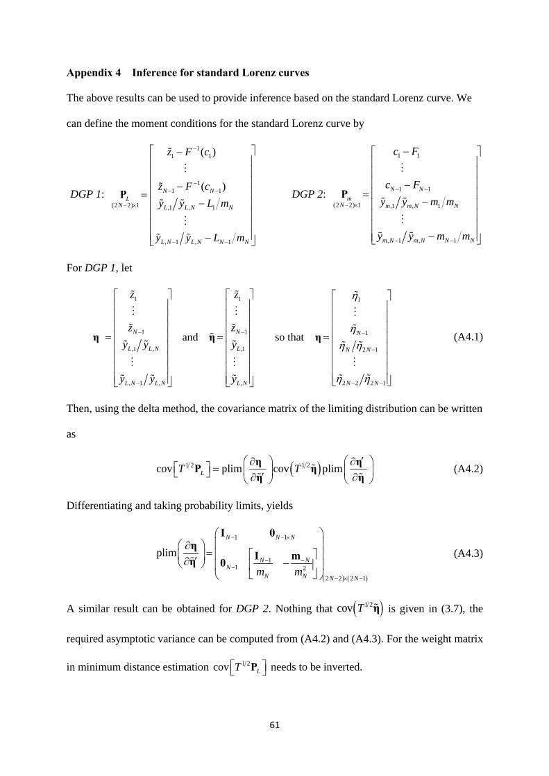
61

Appendix 4 Inference for standard Lorenz curves

The above results can be used to provide inference based on the standard Lorenz curve. We

can define the moment conditions for the standard Lorenz curve by

DGP 1:

11 1

11 1

(2 2) 1 ,1 , 1

, 1 , 1

( )

( )N NL

N L L N N

L N L N N N

z F c

z F c

y y L m

y y L m

P

DGP 2:

1 1

1 1

(2 2) 1 ,1 , 1

, 1 , 1

N N

mN m m N N

m N m N N N

c F

c F

y y m m

y y m m

P

For DGP 1, let

1 1 1

1 1 1

,1 , ,1 2 1

, 1 , , 2 2 2 1

and so thatN N N

L L N L N N

L N L N L N N N

z z

z z

y y y

y y y

η η η

(A4.1)

Then, using the delta method, the covariance matrix of the limiting distribution can be written

as

1 2 1 2cov plim cov plimLT T

η ηP η

η η

(A4.2)

Differentiating and taking probability limits, yields

1 1

11 2

2 2 2 1

plim

N N N

N NN

N N N Nm m

I 0η

I mη 0 (A4.3)

A similar result can be obtained for DGP 2. Nothing that 1 2cov T η is given in (3.7), the

required asymptotic variance can be computed from (A4.2) and (A4.3). For the weight matrix

in minimum distance estimation 1 2cov LT P needs to be inverted.

62

Appendix 5 Lorenz curves with individual data

Proof of Proposition 8: In Proposition 1 we were concerned with the consistency and

asymptotic normality of the minimum distance estimator that considers both the quantile

function and the Lorenz curve. In Proposition 8 we focus on only the conditions for the

quantile function. If, for the moment, we consider a fixed number of groups, the proof for

consistency of the estimator in the first line in (8.1) and its asymptotic normality in (8.2) is

similar to that of Proposition 1. The following assumptions are required.

1) 10( ;F c is differentiable with respect to c and 1

00 ( ; )F c c over (0,1).

2) Compactness: 0 where the parameter space is compact.

3) Identification: 10( ; z F c 0 where plimz z .

4) Continuity: 1( ;F c is continuous over .

5) 0 is an interior point of

6) 1( ;F c is finite and continuously differentiable in a neighbourhood of 0 .

7) 1 1

0 0,11

; ) ; )L

F (c F (cW

is non-singular.

The proposition is also true when the number of groups increases with the sample size,

as is the case with individual data, but some of the underlying assumptions need to be

checked to ensure they can be satisfied. The main assumption to check for consistency is the

uniform convergence assumption. In Proposition 1 where we have a finite number of groups

it is implied by other assumptions. Here we show that it is still implied by the other

assumptions, even for the individual observations case.

Let ( )Q be the objective function; we must find a 0 ( )Q where

0sup | ( ) ( ) | 0pQ Q and 0 is the unique minimiser of 0 ( )Q . Define 0 ( )Q as

63

1 10 ,11( ) ( ; ( ; 1LQ z F c W z F c . First note that this function is minimised at 0

. Second, using the triangular inequality we can write

0 0 ,11

1 1 1,11 ,11 ,11

( ) ( ) 1

2 ( ; ( ; ( ;

L

L L L

Q Q

z z W z z

z F c W z z F c W W F c

Each term on the right-hand side converges to zero for any when the sample size goes

to infinity. For the first term, note that, for every N , 2,11 ( 1)L N T z z W z z and

when N grows we have 2 ( 1) 1N Tc - . For the second term note that again, for every N ,

we have 0 z z and lastly we assume ,11 ,11 0L L W W for every N .

For asymptotic normality we start with the first order conditions:

1

1,11

ˆ( ; ˆ( ;ˆ L

F cW z F c 0

Using a Taylor expansion we can write

1 1

1,11 0 0

ˆ( ; ( ; ˆ( ;ˆ L

F c F cW z F c 0

where is a mean value, i.e., 0ˆ(1 ) = + - for some 0 1 . Solving in terms of

( )0ˆ - , we obtain

1

1 1 11

0 ,11 ,11 0

ˆ( ; ( ; ( ;ˆ ( ;ˆ L LT T

F c F c F cW W z F c

Let

11 10 0

,110 0

( ; ( ;L

F c F cV W

. Because ( )10 ,11( ; ( , )LT Nz F c 0 Ω-- for every

N , we can write

64

1 1

0 00 ,11 ,11 ,11

0 0

( ; ( ;ˆ , L L LT N

F c F c0 V W Ω W V

To obtain this result, we have used standard probability limit rules, uniform continuity of

1( ;F c

-¶¶

over , and the Slutsky theorem. Note further that that we have ,11 ,11L LW Ω I= as

long as ,11LΩ is an invertible matrix for every N . We see below that this is in fact the case.

Thus, we can write ( ) ( )0ˆ ,T N 0 V- .

To derive the weight matrix in (8.3), we note, from (3.2) that

1

1 1 1 12

1 1 1

1,11 ,11

1 1 1 12

1 1 1

(1 ) (1 )

( ) ( ) ( )

[ ( )] [ ( )]

(1 ) (1 )

( ) ( ) ( )

N

N

L L

N N N

N N

c c c c

f z f z f z

D D

c c c c

f z f z f z

W f z A f z

where, using direct multiplication, we can show that

2 0

1 0 2 1 2 1

2 1

1

2

1 1 1 2

1

( )( ) ( )

2 11

( ) 1

1 1( ) 1 2

1

( ) ( )( )

N N

N N

N N N N N N

c c

c c c c c c

c cN

c c

c c

c c c c c c

A

The right hand side is true if 1 ,2 , , ( 1)N N N N c , 0 0c and 1Nc as is the case

with individual data. Noting that 1

1( ; )

( , )ii i

f zF c c

proves (8.3).

Proposition 9

To prove Proposition 9 we provide a series of lemmas:

65

Lemma 5: Let 1( )H θ define a set of N moment conditions, 1W be the corresponding optimal

GMM weight matrix, and θ be the optimal GMM estimator, with asymptotic covariance

matrix 1

1 11

1ˆcovT

H H

θ Wθ θ

. Suppose there is also another M set of moment

conditions ( )H θ where we can write 2 1( ) ( )H θ H H θ . If M N and 2 1 H H evaluated

at 0θ is invertible, then ˆˆ ˆcov cov

θ θ where ˆθ is the optimal GMM estimator

corresponding to the moment conditions ( )H θ .

Proof: First note that using minimum distance estimation theory and the delta method, the

optimal weight matrix and the asymptotic covariance matrix for ˆθ can be written as

1 1

1 12 2 2 21 1

1 1 1 1

cov[ ( )] cov( )

H H H HW H θ H W

H H H H

1

1ˆcov

T

H Hθ W

θ θ

Using the chain rule we can write

11

11 2 2 2 2 11

1 1 1 1

1ˆcov

T

H H H H H Hθ W

θ H H H H θ

If 2 1 H H is invertible, then it follows that that ˆˆ ˆcov cov

θ θ .

Lemma 6: Consider the model in (4.5) with moment conditions ( ; )

( ; )mm

c F zH

y m z

where the bounds are defined by 1( ; )iz F i N . If in the variance formula N T , the

covariance matrix of the GMM estimator for approaches the Cramer-Rao lower bound, i.e.,

11ln ln

lim m mT m E

H H f fW

66

Proof: This Lemma is proved in several steps:

(i) The optimal GMM estimator for from the moment conditions in Lemma 6 has

the same asymptotic covariance as the GMM estimator for the following problem

2

c κ c κΗ

y y c μ κ

where 1y y y , 1c c c

, y y c

, and μ κ .

(ii) Let be the optimal GMM estimator from using 2Η . Its asymptotic

covariance matrix is given by

11ˆcov( )T

where

1

Ni j i j

ij v

These first two steps can be proved using Lemma 5 and the results from Griffiths and

Hajargasht (2015).

(iii) It can be shown that

(a)

21

ln lnlim ( )

( )

Ni j i j

Ni j

f f f ff x dx E

f x

(b)

1

lim 0N

i j

N v

To prove (a), note that 1

1 1( ; ) ( ; )F z F z

N N N

. Thus, we can write:

11

1 1 1 1

( ; ) ( ; )1 ( ; ) ( ; )lim =lim

( ; ) ( ; ) ( ; ) ( ; )

N Ni j j ji i

N N

F z F zF z F z

N F z F z F z F z

Applying Taylor’s theorem to both the numerator and the denominator of the following terms

and assuming the necessary conditions on existence and boundedness of the derivatives of the

density function f we can show that

67

11

1 1

( ; ) (1 )( ; ) ( ; )

( ; ) ( ; ) ( ; ) (1 )ii i

f z O NF z F z

F z F z f z O N

Assuming 1( , ) 0f z , some further manipulations lead to

1 1

1 1 1 1

1 ( , ) ( , )lim lim

( , ) ( , )

N Ni j i i

N N

f z f z

N f z f z

Noting that 11 ( 1)z F N , and using definition of a Riemann-Stieltjes integral, it can

be seen that

1

ln lnlim

Ni j

Ni j

f fE

which proves (iii)(a). Using a similar argument, one can prove (iii)(b).

Lemma 7: Consider the optimal GMM estimator in (8.1) from the moment conditions

1( ; ) H z F c . As T , the variance of approaches the Cramer-Rao lower bound.

Proof: Using results in the proof of Proposition 8, and recognising that ( ;i ic F z we have

11 1

,11

1 ( ; ( ; )ˆcov LT

F c F cW

where

1

,11 [ ( ; )] ( ; ) ( ; ) ( ; ) [ ( ; )]L D D D

W f z F z F z F z f z

From Lemma 2,

11( ; ( ; )[ ( ; )]D

F c F zf z

And thus,

1

11 ( ; ) ( ; )ˆcov ( ; ) ( ; ) ( ; )DT

F z F zF z F z F z

Again using Lemma 5 it can be shown that

68

11ˆ ˆcov( ) ( )T

where 1

Ti j

ij

We showed in Lemma 6 that this quantity converges to the Cramer-Rao lower bound.

Lemma 8: Consider the Lorenz curve estimation problem (8.4) with the moment conditions

H y L c and individual data. As the number of observations approaches infinity, the

variance of the optimal GMM estimator for approaches the Cramer-Rao lower bound.

Proof: According to Proposition 7, the asymptotic covariance for the optimal GMM

estimator for this problem is equal to the asymptotic covariance of the optimal GMM

estimator for the problem considered in Lemma 6. We showed in Lemma 6 that the latter

asymptotic covariance converges to Cramer-Rao lower bound which proves the lemma.

Proof of Proposition 9: Lemma 7, Lemma 8 and the fact that asymptotic covariance of the

maximum likelihood estimator is equal to Cramer-Rao lower bound proves the proposition.