
ES360 Introduction to Controls Engineering
152
Revision 2.2 December 2006 ES360 Introduction to Controls Engineering Lessons 1 to 11 Name:______________________ Section:__________ Instructor:__________________ Lesson Topic MATLAB Files Required 1a Complex Number & Quadratic Equation Review 1b Block Diagram Reduction 1c Introduction to the Frequency Domain wavgen.m 2a Basic Element Types 2b First Order Transfer Functions 3a Input Types and the Final Value Theorem 3b Second Order Systems’ Time Response MATLAB Only 4 Second Order Time Response Calculations 5a Graphical Analysis of Second Order Responses 5b Measurement of a Second Order Response 5c Modeling the F/A-18 Landing Gear f18.mdl & f18landing.m 6a Introduction to Feedback 6b Introduction to Controllers 7 Modeling and Feedback of a Gun Turret MATLAB & SIMULINK 8 Disturbances and Actuator Limitations gun_barrel_elev.mdl 9 PID Control of a Generator Set generator.mdl 10 PID Control and Discrete Sampling cruise_missile.mdl 11 Hardware Implementation of PID Speed Control United States Naval Academy Weapons and Systems Engineering Department LT Roger Cortesi, USN
Transcript of ES360 Introduction to Controls Engineering
Revision 2.2 December 2006
ES360 Introduction to Controls Engineering
Lessons 1 to 11
Name:______________________ Section:__________
Instructor:__________________
Lesson Topic MATLAB Files Required
1a Complex Number & Quadratic Equation Review
1b Block Diagram Reduction
1c Introduction to the Frequency Domain wavgen.m
2a Basic Element Types
2b First Order Transfer Functions
3a Input Types and the Final Value Theorem
3b Second Order Systems’ Time Response MATLAB Only
4 Second Order Time Response Calculations
5a Graphical Analysis of Second Order Responses
5b Measurement of a Second Order Response
5c Modeling the F/A-18 Landing Gear f18.mdl & f18landing.m
6a Introduction to Feedback
6b Introduction to Controllers
7 Modeling and Feedback of a Gun Turret MATLAB & SIMULINK
8 Disturbances and Actuator Limitations gun_barrel_elev.mdl
9 PID Control of a Generator Set generator.mdl
10 PID Control and Discrete Sampling cruise_missile.mdl
11 Hardware Implementation of PID Speed Control
United States Naval Academy Weapons and Systems Engineering Department
LT Roger Cortesi, USN

Classroom Door Combination
ES360 Introduction to Controls Engineering
MATLAB and SIMULINK Help
Page 1 of 6
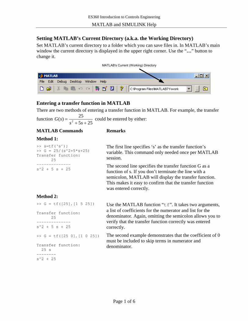
Setting MATLAB’s Current Directory (a.k.a. the Working Directory) Set MATLAB’s current directory to a folder which you can save files in. In MATLAB’s main window the current directory is displayed in the upper right corner. Use the “…” button to change it.
MATLAB's Current (Working) Directory
Entering a transfer function in MATLAB There are two methods of entering a transfer function in MATLAB. For example, the transfer
function 255
25)( 2 ++=
sssG could be entered by either:
MATLAB Commands Remarks
Method 1: >> s=tf(‘s’); >> G = 25/(s^2+5*s+25) Transfer function: 25 -------------- s^2 + 5 s + 25
The first line specifies ‘s’ as the transfer function’s variable. This command only needed once per MATLAB session.
The second line specifies the transfer function G as a function of s. If you don’t terminate the line with a semicolon, MATLAB will display the transfer function. This makes it easy to confirm that the transfer function was entered correctly.
Method 2: >> G = tf([25],[1 5 25]) Transfer function: 25 -------------- s^2 + 5 s + 25 >> G = tf([25 0],[1 0 25]) Transfer function: 25 s -------- s^2 + 25
Use the MATLAB function “tf”. It takes two arguments, a list of coefficients for the numerator and list for the denominator. Again, omitting the semicolon allows you to verify that the transfer function correctly was entered correctly.
The second example demonstrates that the coefficient of 0 must be included to skip terms in numerator and denominator.

ES360 Introduction to Controls Engineering
MATLAB and SIMULINK Help
Page 2 of 6
Starting SIMULINK SIMULINK can be started by:
1) Opening a SIMULINK model file (model files use the .mdl extension).
2) Starting MATLAB and clicking on the icon in the tool bar.
The SIMULINK Library Browser SIMULINK models are made up of different elements connected in a block diagram. The SIMULINK Library Browser is catalog of all the elements available to the model.
View the library browser with the icon or by selecting the “Library Browser” menu option in the “View” menu of a model file.
Creating a New SIMULINK Model
Open the SIMULINK Library Browser. Click on the “New Model” icon or select “New… → Model File…” from the Library browser’s “File” menu. This will open a blank model window.
Setting the Start and Stop Time of a Simulation The start and stop time of a simulation is set in the model file’s “Configuration Parameters” window. (“Simulation” menu → “Configuration Parameters”, or press Ctrl-E)
SIMULINK Printing Problems Sometime when printing a plot generated by SIMULINK, the line will be printed in a very light shade of grey. This is makes it very difficult to read the plot. This happens when MATLAB sends color data to a black and white printer. The black and white printer prints the yellow line as a very light shade of grey.
To fix this, go to the “general” setting in the preferences window (“File” menu → “Preferences…”). Set “Figure Window Printing” to “Always send as black and white”.
Make sure you use the “File” menu from the SIMULINK model file’s window.
SIMULINK Scope Block NOT Plotting All the Results If a scope block does not seem to be displaying all the results from the simulation, try clicking on the autoscale button at the top of the plot to resize the plot’s axes.
In some simulations the scope block will not plot data at the beginning of the simulation. For example, in a 20 second simulation, it might only plot the last 14 seconds of data. By default a scope block will only display the last 5,000 data points. If the simulation used more that 5,000 data points, then the earlier points will not be plotted.
To change this setting, open the ‘Scope’ Parameters window by clicking on the icon in the top right corner of the scope’s plot. Select the “Data History” tab and uncheck the “Limit data points to last: x” checkbox. You need to make this change to each of the affected scopes.
ES360 Introduction to Controls Engineering
MATLAB and SIMULINK Help
Page 3 of 6
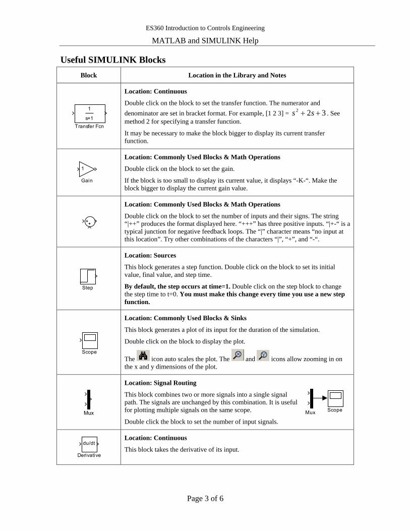
Useful SIMULINK Blocks Block Location in the Library and Notes
1
s+1Transfer Fcn
Location: Continuous
Double click on the block to set the transfer function. The numerator and denominator are set in bracket format. For example, [1 2 3] = 322 ++ ss . See method 2 for specifying a transfer function.
It may be necessary to make the block bigger to display its current transfer function.
1
Gain
Location: Commonly Used Blocks & Math Operations
Double click on the block to set the gain.
If the block is too small to display its current value, it displays “-K-“. Make the block bigger to display the current gain value.
Location: Commonly Used Blocks & Math Operations
Double click on the block to set the number of inputs and their signs. The string “|++” produces the format displayed here. “+++” has three positive inputs. “|+-“ is a typical junction for negative feedback loops. The “|” character means “no input at this location”. Try other combinations of the characters “|”, “+”, and “-“.
Step
Location: Sources
This block generates a step function. Double click on the block to set its initial value, final value, and step time.
By default, the step occurs at time=1. Double click on the step block to change the step time to t=0. You must make this change every time you use a new step function.
Scope
Location: Commonly Used Blocks & Sinks
This block generates a plot of its input for the duration of the simulation.
Double click on the block to display the plot.
The icon auto scales the plot. The and icons allow zooming in on the x and y dimensions of the plot.
Mux
Location: Signal Routing
This block combines two or more signals into a single signal path. The signals are unchanged by this combination. It is useful for plotting multiple signals on the same scope.
Double click the block to set the number of input signals.
du/dt
Derivative
Location: Continuous
This block takes the derivative of its input.
Mux Scope
ES360 Introduction to Controls Engineering
MATLAB and SIMULINK Help
Page 4 of 6
1s
Integrator
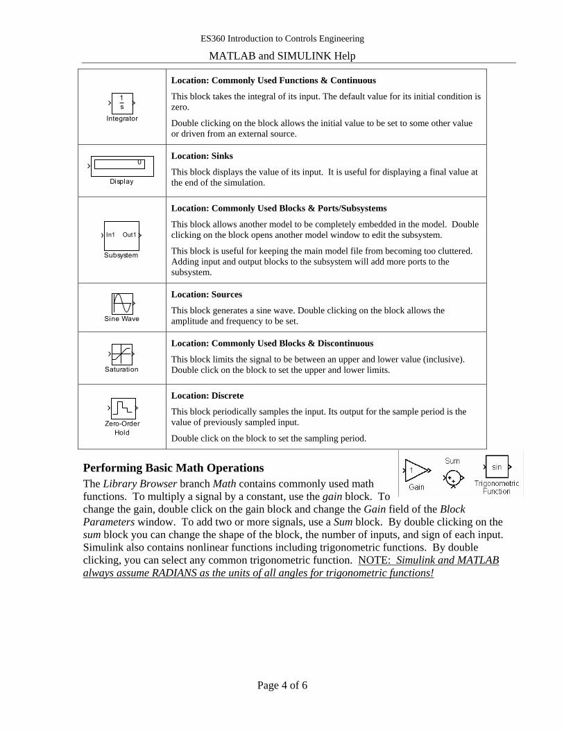
Location: Commonly Used Functions & Continuous
This block takes the integral of its input. The default value for its initial condition is zero.
Double clicking on the block allows the initial value to be set to some other value or driven from an external source.
0
Display
Location: Sinks
This block displays the value of its input. It is useful for displaying a final value at the end of the simulation.
In1 Out1
Subsystem
Location: Commonly Used Blocks & Ports/Subsystems
This block allows another model to be completely embedded in the model. Double clicking on the block opens another model window to edit the subsystem.
This block is useful for keeping the main model file from becoming too cluttered. Adding input and output blocks to the subsystem will add more ports to the subsystem.
Sine Wave
Location: Sources
This block generates a sine wave. Double clicking on the block allows the amplitude and frequency to be set.
Saturation
Location: Commonly Used Blocks & Discontinuous
This block limits the signal to be between an upper and lower value (inclusive). Double click on the block to set the upper and lower limits.
Zero-OrderHold
Location: Discrete
This block periodically samples the input. Its output for the sample period is the value of previously sampled input.
Double click on the block to set the sampling period.
Performing Basic Math Operations The Library Browser branch Math contains commonly used math functions. To multiply a signal by a constant, use the gain block. To change the gain, double click on the gain block and change the Gain field of the Block Parameters window. To add two or more signals, use a Sum block. By double clicking on the sum block you can change the shape of the block, the number of inputs, and sign of each input. Simulink also contains nonlinear functions including trigonometric functions. By double clicking, you can select any common trigonometric function. NOTE: Simulink and MATLAB always assume RADIANS as the units of all angles for trigonometric functions!
ES360 Introduction to Controls Engineering
MATLAB and SIMULINK Help
Page 5 of 6
Basic MATLAB Workspace Commands who lists the names of all variables in the workspace whos lists all variables in the workspace along with their size and data type clear removes all variables from workspace clear name removes the variable name save name saves all variables in the workspace in the disk file name load name loads variables from disk file name into the workspace dir lists the files in the disk current directory
Basic MATLAB Plotting Commands plot(x,y) plots data in vector y versus the data in vector x plot(x,y,’s’) plots data in vector y versus x with line attributes ’s’ plot(x1,y1,’s1’,x2,y2,’s2’) plots y1 versus x1 with line attributes ’s1’
and y2 versus x2 with line attributes ’s2’
The following table summarizes basic line attributes. An attribute string can contain one character from each column:
Basic MATLAB Line Attributes
Color Marker Style Line Style b blue . point - solid g green o circle : dotted r red x x-mark -. dashdot c cyan + plus -- dashed m magenta * star y yellow s square k black d diamond
Your can create and manipulate multiple figure windows using the following commands: figure(n) switch to the nth figure window, making it the active figure, create figure window n if necessary hold on hold active figure so that plot commands are cumulative hold off release active figure hold so that the next plot command erases existing data clf clear the active figure window
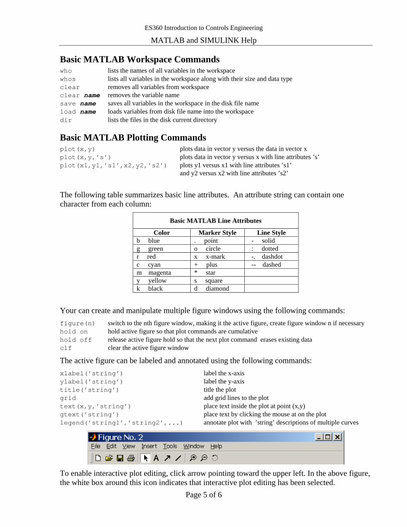
The active figure can be labeled and annotated using the following commands: xlabel(’string’) label the x-axis ylabel(’string’) label the y-axis title(’string’) title the plot grid add grid lines to the plot text(x,y,’string’) place text inside the plot at point (x,y) gtext(’string’) place text by clicking the mouse at on the plot legend(’string1’,’string2’,...) annotate plot with ’string’ descriptions of multiple curves
To enable interactive plot editing, click arrow pointing toward the upper left. In the above figure, the white box around this icon indicates that interactive plot editing has been selected.
ES360 Introduction to Controls Engineering
MATLAB and SIMULINK Help
Page 6 of 6
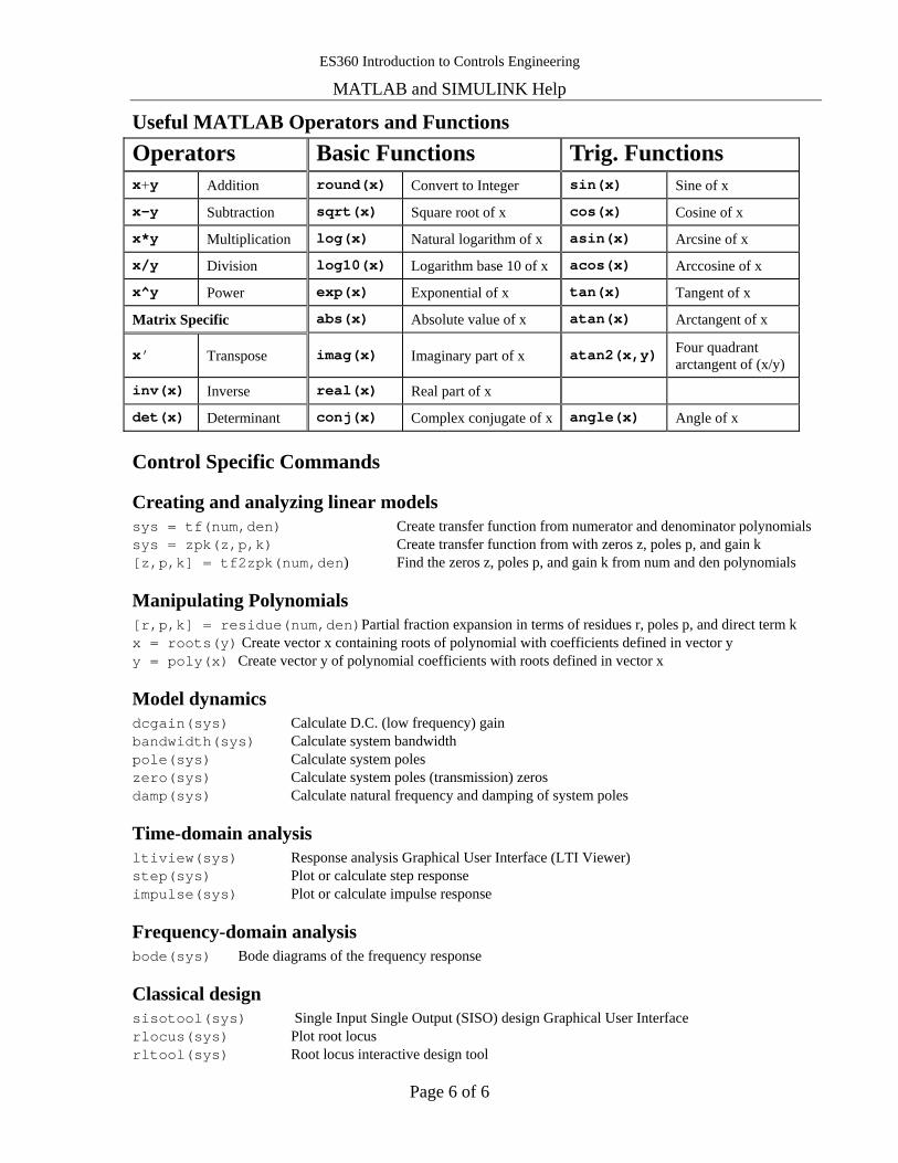
Useful MATLAB Operators and Functions Operators Basic Functions Trig. Functions x+y Addition round(x) Convert to Integer sin(x) Sine of x
x-y Subtraction sqrt(x) Square root of x cos(x) Cosine of x
x*y Multiplication log(x) Natural logarithm of x asin(x) Arcsine of x
x/y Division log10(x) Logarithm base 10 of x acos(x) Arccosine of x
x^y Power exp(x) Exponential of x tan(x) Tangent of x
Matrix Specific abs(x) Absolute value of x atan(x) Arctangent of x
x’ Transpose imag(x) Imaginary part of x atan2(x,y) Four quadrant arctangent of (x/y)
inv(x) Inverse real(x) Real part of x
det(x) Determinant conj(x) Complex conjugate of x angle(x) Angle of x
Control Specific Commands
Creating and analyzing linear models sys = tf(num,den) Create transfer function from numerator and denominator polynomials sys = zpk(z,p,k) Create transfer function from with zeros z, poles p, and gain k [z,p,k] = tf2zpk(num,den) Find the zeros z, poles p, and gain k from num and den polynomials
Manipulating Polynomials [r,p,k] = residue(num,den)Partial fraction expansion in terms of residues r, poles p, and direct term k x = roots(y) Create vector x containing roots of polynomial with coefficients defined in vector y y = poly(x) Create vector y of polynomial coefficients with roots defined in vector x
Model dynamics dcgain(sys) Calculate D.C. (low frequency) gain bandwidth(sys) Calculate system bandwidth pole(sys) Calculate system poles zero(sys) Calculate system poles (transmission) zeros damp(sys) Calculate natural frequency and damping of system poles
Time-domain analysis ltiview(sys) Response analysis Graphical User Interface (LTI Viewer) step(sys) Plot or calculate step response impulse(sys) Plot or calculate impulse response
Frequency-domain analysis bode(sys) Bode diagrams of the frequency response
Classical design sisotool(sys) Single Input Single Output (SISO) design Graphical User Interface rlocus(sys) Plot root locus rltool(sys) Root locus interactive design tool
ES360 Introduction to Controls Engineering
Lesson 1a: Complex Number and Quadratic Equation Review
Page 1 of 2
Complex Numbers Recall that complex numbers have a real and an imaginary part. The imaginary part is usually written as a multiple of i. Where i is the square root of -1. Many texts will use the letter j, instead of i, for the square root of -1.
Complex numbers can be written in either rectangular form, bias += where the real and imaginary components are separate. Or they can be written in polar form as an angle and a magnitude, °∠= dcs .
Addition and subtraction of complex numbers by hand is easier in rectangular form. Multiplication and division of complex numbers by hand is easier in polar form.
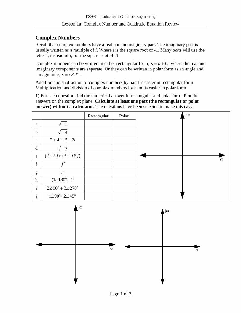
1) For each question find the numerical answer in rectangular and polar form. Plot the answers on the complex plane. Calculate at least one part (the rectangular or polar answer) without a calculator. The questions have been selected to make this easy.
Rectangular Polar
a 1−
b 4−
c ii 2542 −++
d 2−
e )5.03()52( jj +⋅+
f 2j
g 3i
h 2)1801( ⋅°∠
i °∠+°∠ 2703902
j °∠⋅°∠ 452901
σ
jω
σ
jω
σ
jω
ES360 Introduction to Controls Engineering
Lesson 1a: Complex Number and Quadratic Equation Review
Page 2 of 2
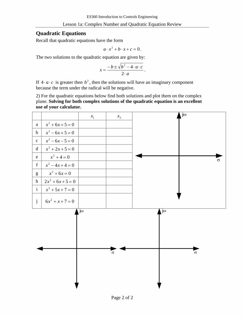
Quadratic Equations Recall that quadratic equations have the form
02 =+⋅+⋅ cxbxa .
The two solutions to the quadratic equation are given by:
acabbx
⋅⋅⋅−±−
=2
42
.
If ca ⋅⋅4 is greater then 2b , then the solutions will have an imaginary component because the term under the radical will be negative.
2) For the quadratic equations below find both solutions and plot them on the complex plane. Solving for both complex solutions of the quadratic equation is an excellent use of your calculator.
1x 2x
a 0562 =++ xx
b 0562 =+− xx
c 0562 =−− xx
d 0522 =++ xx
e 042 =+x
f 0442 =+− xx
g 062 =+ xx
h 0562 2 =++ xx
i 0752 =++ xx
j 076 2 =++ xx
σ
jω
σ
jω
σ
jω
ES360 Introduction to Controls Engineering
Lesson 1b: Block Diagrams
Page 1 of 10
Block Diagrams
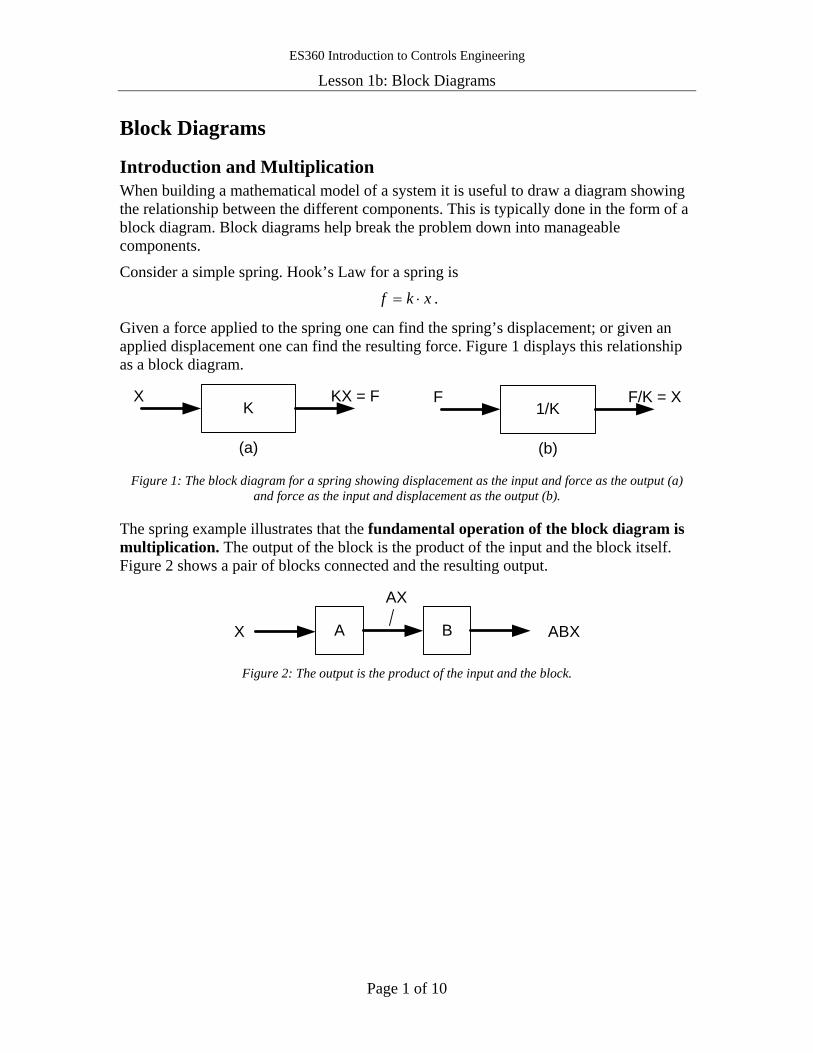
Introduction and Multiplication When building a mathematical model of a system it is useful to draw a diagram showing the relationship between the different components. This is typically done in the form of a block diagram. Block diagrams help break the problem down into manageable components.
Consider a simple spring. Hook’s Law for a spring is
xkf ⋅= .
Given a force applied to the spring one can find the spring’s displacement; or given an applied displacement one can find the resulting force. Figure 1 displays this relationship as a block diagram.
KX KX = F
(a)
1/KF F/K = X
(b)
Figure 1: The block diagram for a spring showing displacement as the input and force as the output (a) and force as the input and displacement as the output (b).
The spring example illustrates that the fundamental operation of the block diagram is multiplication. The output of the block is the product of the input and the block itself. Figure 2 shows a pair of blocks connected and the resulting output.
AX B
AX
ABX
Figure 2: The output is the product of the input and the block.
ES360 Introduction to Controls Engineering
Lesson 1b: Block Diagrams
Page 2 of 10
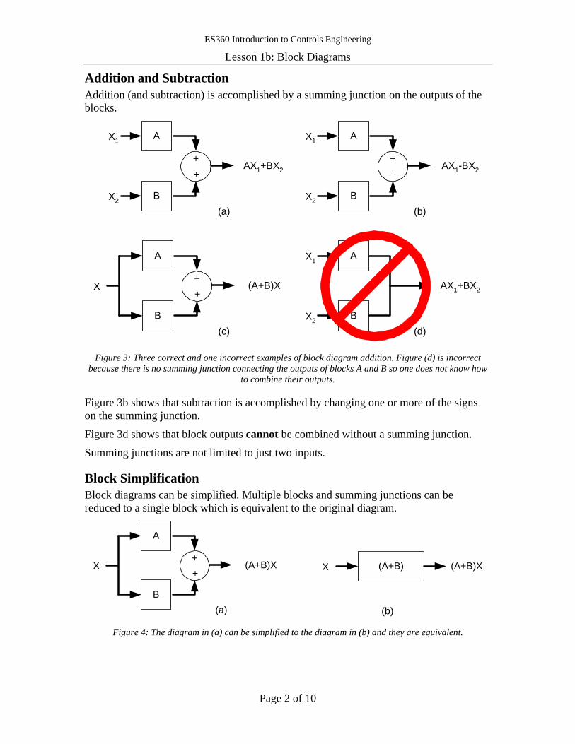
Addition and Subtraction Addition (and subtraction) is accomplished by a summing junction on the outputs of the blocks.
A
B
++
X (A+B)X
(c)
AX1
BX2
AX1+BX2
(d)
AX1
B
+-
X2
AX1-BX2
(b)
AX1
B
++
X2
AX1+BX2
(a)
Figure 3: Three correct and one incorrect examples of block diagram addition. Figure (d) is incorrect
because there is no summing junction connecting the outputs of blocks A and B so one does not know how to combine their outputs.
Figure 3b shows that subtraction is accomplished by changing one or more of the signs on the summing junction.
Figure 3d shows that block outputs cannot be combined without a summing junction.
Summing junctions are not limited to just two inputs.
Block Simplification Block diagrams can be simplified. Multiple blocks and summing junctions can be reduced to a single block which is equivalent to the original diagram.
A
B
++
X (A+B)X
(a)
(A+B)X
(b)
(A+B)X
Figure 4: The diagram in (a) can be simplified to the diagram in (b) and they are equivalent.
ES360 Introduction to Controls Engineering
Lesson 1b: Block Diagrams
Page 3 of 10
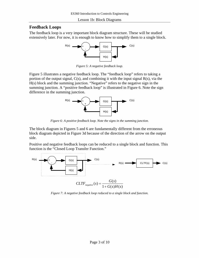
Feedback Loops The feedback loop is a very important block diagram structure. These will be studied extensively later. For now, it is enough to know how to simplify them to a single block.
G(s)R(s) C(s)+-
H(s)
Figure 5: A negative feedback loop.
Figure 5 illustrates a negative feedback loop. The “feedback loop” refers to taking a portion of the output signal, C(s), and combining it with the input signal R(s), via the H(s) block and the summing junction. “Negative” refers to the negative sign in the summing junction. A “positive feedback loop” is illustrated in Figure 6. Note the sign difference in the summing junction.
G(s)R(s) C(s)++
H(s)
Figure 6: A positive feedback loop. Note the signs in the summing junction.
The block diagram in Figures 5 and 6 are fundamentally different from the erroneous block diagram depicted in Figure 3d because of the direction of the arrow on the output side.
Positive and negative feedback loops can be reduced to a single block and function. This function is the “Closed Loop Transfer Function.”
G(s)R(s) C(s)+-
H(s)
CLTF(s) C(s)R(s)
)()(1)()(
sHsGsGsCLTFnegative +
=
Figure 7: A negative feedback loop reduced to a single block and function.
ES360 Introduction to Controls Engineering
Lesson 1b: Block Diagrams
Page 4 of 10
G(s)R(s) C(s)++
H(s)
CLTF(s) C(s)R(s)
)()(1)()(
sHsGsGsCLTFpositive −
=
Figure 8: A positive feedback loop reduced to a single block and function.
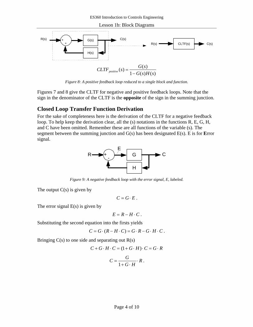
Figures 7 and 8 give the CLTF for negative and positive feedback loops. Note that the sign in the denominator of the CLTF is the opposite of the sign in the summing junction.
Closed Loop Transfer Function Derivation For the sake of completeness here is the derivation of the CLTF for a negative feedback loop. To help keep the derivation clear, all the (s) notations in the functions R, E, G, H, and C have been omitted. Remember these are all functions of the variable (s). The segment between the summing junction and G(s) has been designated E(s). E is for Error signal.
GR C+-
H
E
Figure 9: A negative feedback loop with the error signal, E, labeled.
The output C(s) is given by
EGC ⋅= .
The error signal E(s) is given by
CHRE ⋅−= .
Substituting the second equation into the firsts yields
CHGRGCHRGC ⋅⋅−⋅=⋅−⋅= )( .
Bringing C(s) to one side and separating out R(s)
RGCHGCHGC ⋅=⋅⋅+=⋅⋅+ )1(
RHG
GC ⋅⋅+
=1
.
ES360 Introduction to Controls Engineering
Lesson 1b: Block Diagrams
Page 5 of 10
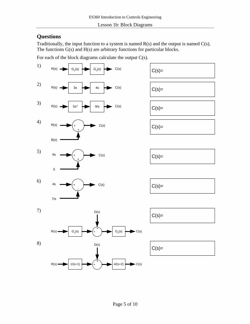
Questions Traditionally, the input function to a system is named R(s) and the output is named C(s). The functions G(s) and H(s) are arbitrary functions for particular blocks.
For each of the block diagrams calculate the output C(s).
1) G1(s) G2(s)R(s) C(s)
C(s)=
2)
3s 4sR(s) C(s)
C(s)=
3)
5s2 9/sR(s) C(s)
C(s)=
4)
++
C(s)R(s)
B(s)
C(s)=
5) +
+C(s)6s
5
C(s)=
6) +
-C(s)4s
7/s
C(s)=
7)
G1(s) G2(s)R(s) C(s)++
D(s)C(s)=
8)
1/(s+1) 4/(s+2)R(s) C(s)++
D(s)C(s)=
ES360 Introduction to Controls Engineering
Lesson 1b: Block Diagrams
Page 6 of 10
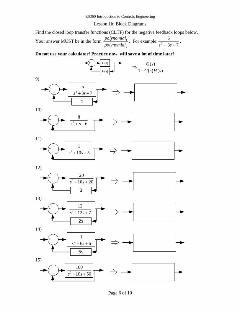
Find the closed loop transfer functions (CLTF) for the negative feedback loops below.
Your answer MUST be in the form 2
1
polynomialpolynomial . For example:
735
2 ++ ss.
Do not use your calculator! Practice now, will save a lot of time later!
G(s)+-
H(s)
)()(1)(
sHsGsG
+⇒
9)
+-
1
735
2 ++ ss
10)
+- 6
82 ++ ss
11)
+- 510
12 ++ ss
12)
+-
3
201020
2 ++ ss
13)
+-
2s
71212
2 ++ ss
14)
+-
5s
661
2 ++ ss
15)
+- 5010
1002 ++ ss
ES360 Introduction to Controls Engineering
Lesson 1b: Block Diagrams
Page 7 of 10
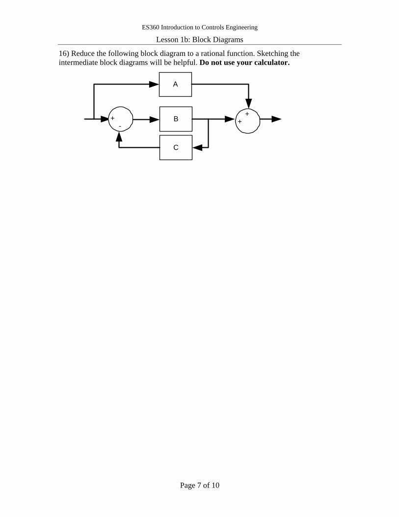
16) Reduce the following block diagram to a rational function. Sketching the intermediate block diagrams will be helpful. Do not use your calculator.
B+-
C
++
A
ES360 Introduction to Controls Engineering
Lesson 1b: Block Diagrams
Page 8 of 10
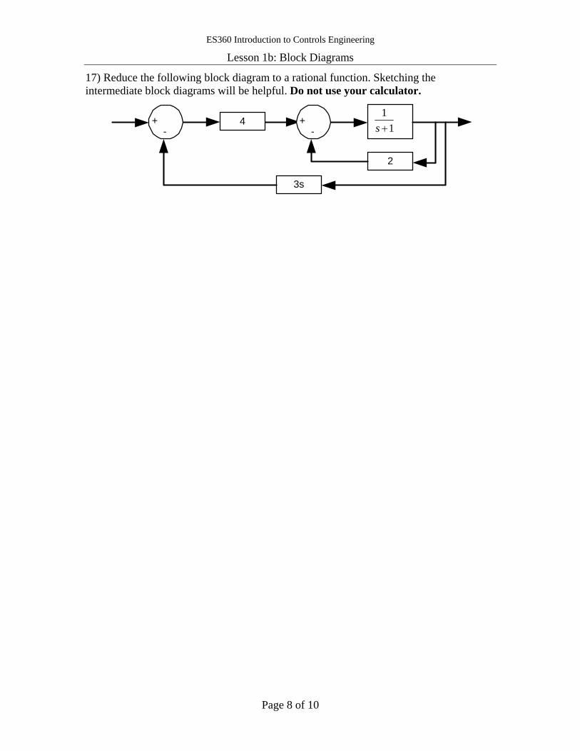
17) Reduce the following block diagram to a rational function. Sketching the intermediate block diagrams will be helpful. Do not use your calculator.
+-
2
+-
4
3s
11+s
ES360 Introduction to Controls Engineering
Lesson 1b: Block Diagrams
Page 9 of 10
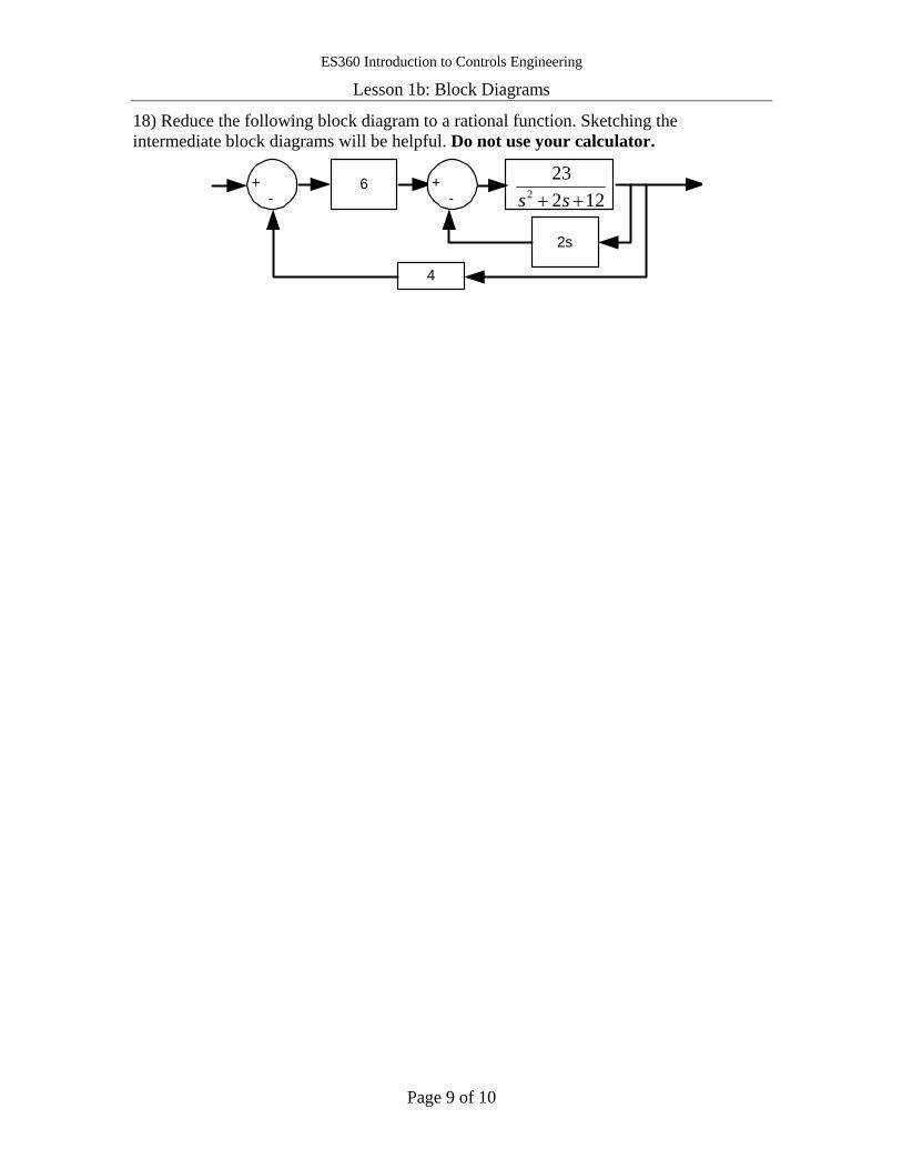
18) Reduce the following block diagram to a rational function. Sketching the intermediate block diagrams will be helpful. Do not use your calculator.
+-
2s
+-
6
4
12223
2 ++ ss
ES360 Introduction to Controls Engineering
Lesson 1b: Block Diagrams
Page 10 of 10
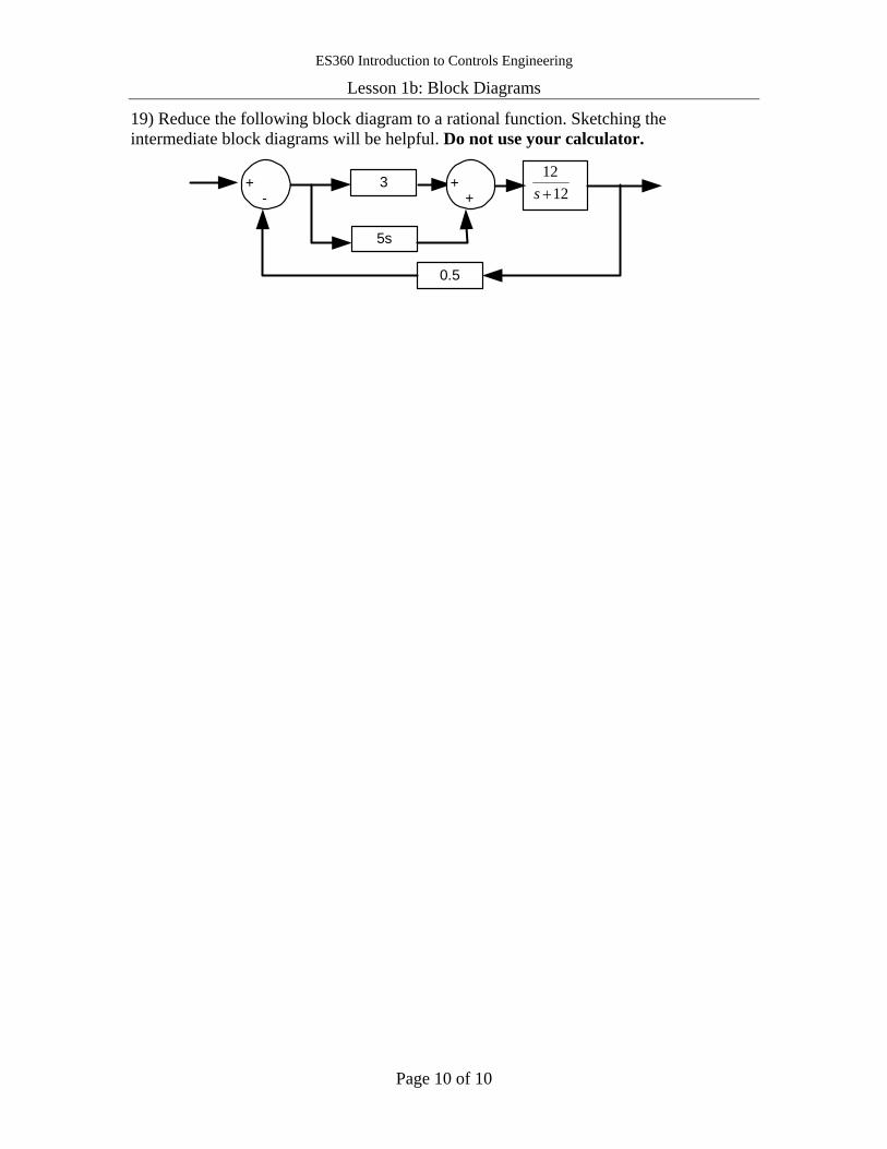
19) Reduce the following block diagram to a rational function. Sketching the intermediate block diagrams will be helpful. Do not use your calculator.
++
5s
+-
3
0.5
1212+s
ES360 Introduction to Controls Engineering
Lesson 1c: Wave Forms and the Frequency Domain
Page 1 of 4
Frequency Domain & Building Complicated Wave Forms
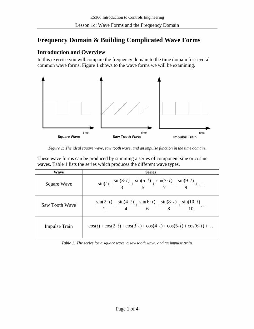
Introduction and Overview In this exercise you will compare the frequency domain to the time domain for several common wave forms. Figure 1 shows to the wave forms we will be examining.
timeSquare Wave
timeSaw Tooth Wave
timeImpulse Train
Figure 1: The ideal square wave, saw tooth wave, and an impulse function in the time domain.
These wave forms can be produced by summing a series of component sine or cosine waves. Table 1 lists the series which produces the different wave types.
Wave Series
Square Wave K+⋅
+⋅
+⋅
+⋅
+9
)9sin(7
)7sin(5
)5sin(3
)3sin()sin( ttttt
Saw Tooth Wave K10
)10sin(8
)8sin(6
)6sin(4
)4sin(2
)2sin( ttttt ⋅+
⋅+
⋅+
⋅+
⋅
Impulse Train K+⋅+⋅+⋅+⋅+⋅+ )6cos()5cos()4cos()3cos()2cos()cos( tttttt
Table 1: The series for a square wave, a saw tooth wave, and an impulse train.
ES360 Introduction to Controls Engineering
Lesson 1c: Wave Forms and the Frequency Domain
Page 2 of 4
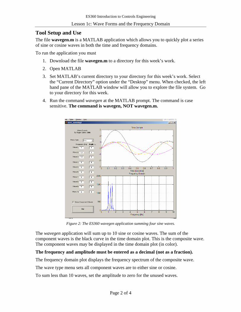
Tool Setup and Use The file wavegen.m is a MATLAB application which allows you to quickly plot a series of sine or cosine waves in both the time and frequency domains.
To run the application you must
1. Download the file wavegen.m to a directory for this week’s work.
2. Open MATLAB
3. Set MATLAB’s current directory to your directory for this week’s work. Select the “Current Directory” option under the “Desktop” menu. When checked, the left hand pane of the MATLAB window will allow you to explore the file system. Go to your directory for this week.
4. Run the command wavegen at the MATLAB prompt. The command is case sensitive. The command is wavegen, NOT wavegen.m.
Figure 2: The ES360 wavegen application summing four sine waves.
The wavegen application will sum up to 10 sine or cosine waves. The sum of the component waves is the black curve in the time domain plot. This is the composite wave. The component waves may be displayed in the time domain plot (in color).
The frequency and amplitude must be entered as a decimal (not as a fraction). The frequency domain plot displays the frequency spectrum of the composite wave.
The wave type menu sets all component waves are to either sine or cosine.
To sum less than 10 waves, set the amplitude to zero for the unused waves.
ES360 Introduction to Controls Engineering
Lesson 1c: Wave Forms and the Frequency Domain
Page 3 of 4
Questions 1) On the axis below sketch the frequency response for a single sine wave. Sketch what happens as you change the frequency and amplitude of the wave.
frequency 2) Using the wavegen command, plot each wave type in the time and frequency domains. Make a sketch of the plots on the axis below:
Square Wave
time
frequency
ES360 Introduction to Controls Engineering
Lesson 1c: Wave Forms and the Frequency Domain
Page 4 of 4
Saw Tooth Wave
time
frequency Impulse
time
frequency 3) As you add more terms to the series (i.e. you sum more component waves) what happens to the composite wave in the time and frequency domains?
ES360 Introduction to Controls Engineering
Lesson 2a: Basic Element Types
Page 1 of 5
Basic Element Types
Introduction, the Mass Spring Damper The three basic elements in system modeling are:
1. A kinetic energy storage element
2. A potential energy storage element
3. An energy dissipative element
Most real system can be modeled as combinations of these three elements.
Mass (M)
Spring (K)
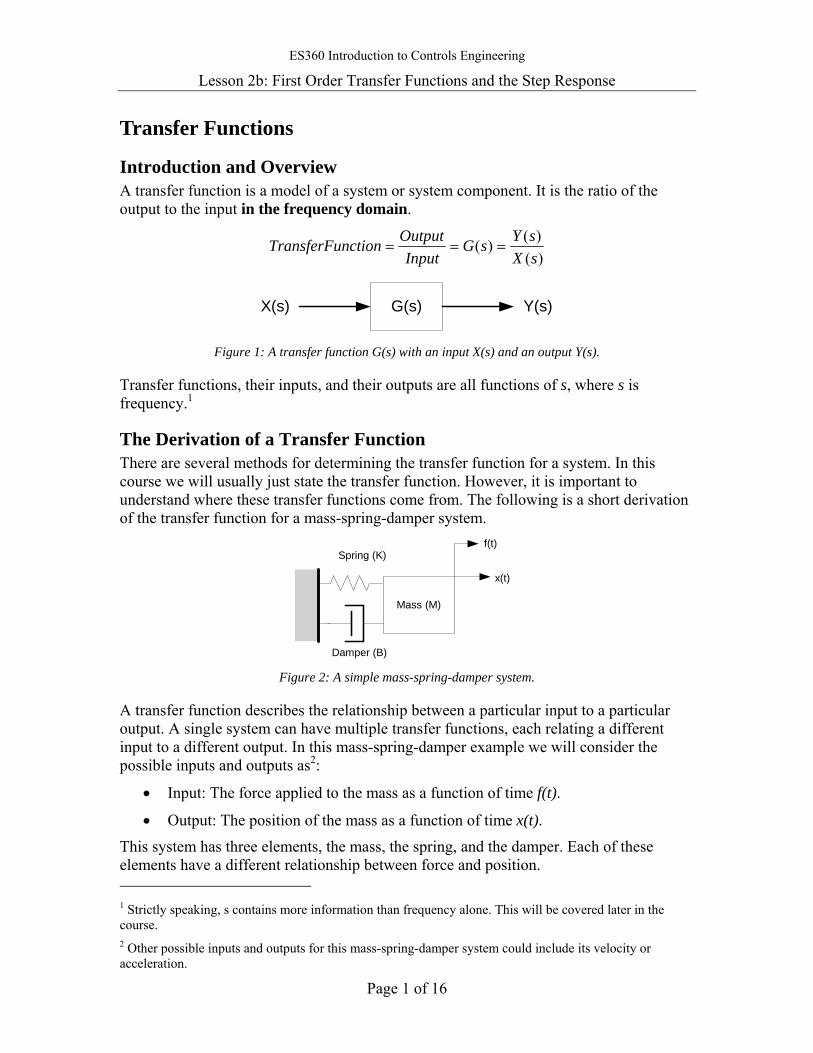
Damper (B) Figure 1: A simple mass spring damper system. This system has each of the three basic elements.
Figure 1 shows a simple mass spring damper system. The spring is the potential energy storage element, storing energy in its compression. The mass is the kinetic energy storage element, storing energy in its momentum. The damper (a source of friction) is the energy dissipative element.
Mass (M)
Spring (K)Damper (B)
(a) (c)(b)
Figure 2: The mass spring damper model (a) can be applied to systems which clearly have separate mass spring damper components (b) and those that do not (c).
It is important to understand that these three elements are concepts, and not necessarily individual physical components of the system. For example, a mass hanging from a Slinky can be modeled using the above mass spring damper model. In this case the three elements are distinct physical parts of the system.
A cantilevered beam sticking out of a wall can also be modeled using the same three components. In this case the there is only one physical part (the beam), but the beam exhibits characteristics of all three elements (mass, springiness, and friction).
In both cases applying a force to the system (hitting it with a hammer) will cause it to vibrate back and forth until the friction dampens out the oscillations.

ES360 Introduction to Controls Engineering
Lesson 2a: Basic Element Types
Page 2 of 5
Basic Elements in Other Energy Domains The rotational, electrical, fluid and thermal1 energy domains all have similar elements to the mechanical translational domain discussed above.
Domain Kinetic Energy Potential Energy Dissipative Mechanical
(translational) Mass Spring Damper
Mechanical (rotational) Rotational Inertia Spring Damper
Electrical Inductor Capacitor Resistor
Fluid Fluid Mass Fluid Capacitance (a reservoir)
Fluid Resistance
Thermal Thermal Capacitance (Thermal Mass)
Thermal Resistance
Table 1: Basic element types for five different energy domains.
Energy Transfer Between Different Energy Domains Real objects are normally composed of several different energy domains (mechanical, electrical, fluid, etc.). These different domains interact with each other by moving energy between them. In addition to the conceptual elements described in Table 1, there are many physical elements which transfer energy between the different energy domains.
Complete the table below. Domain 1 Domain 2 Objects that Transfer Energy from Domain 1 to Domain 2
Rotational Translational
Rotational Electrical
Rotational Fluid
Fluid Translational
Electrical Thermal
Electrical Rotational
Rotational Thermal
1 The behavior of thermal systems is slightly different from the other four energy domains.
The thermal capacitance of a system stores both kinetic and potential energy. The kinetic energy is stored in the translational motion of the atoms. The potential energy is associated with the intermolecular attractive and repulsive forces.
In the other systems the dissipative elements convert motion to heat via friction or electrical resistance. In the thermal system the dissipative element delays the propagation of heat in time and space.

ES360 Introduction to Controls Engineering
Lesson 2a: Basic Element Types
Page 3 of 5
Questions In the images below label the energy storage elements (kinetic and potential) and the dissipative elements. Label any conversions between energy domains.
Hydro-electric Dam
Suspension Bridge
Mountain Bike

ES360 Introduction to Controls Engineering
Lesson 2a: Basic Element Types
Page 4 of 5
Squash Racquet and Ball
DC Electric Motor and Gear Box
Bungee Jumping

ES360 Introduction to Controls Engineering
Lesson 2a: Basic Element Types
Page 5 of 5
Solar Panels for Heating Water
Tanqueray™
Steam Engine

ES360 Introduction to Controls Engineering Lesson 2b: First Order Transfer Functions and the Step Response
Page 1 of 16
Transfer Functions
Introduction and Overview A transfer function is a model of a system or system component. It is the ratio of the output to the input in the frequency domain.
)()()(
sXsYsG
InputOutputnctionTransferFu ===
G(s)X(s) Y(s)
Figure 1: A transfer function G(s) with an input X(s) and an output Y(s).
Transfer functions, their inputs, and their outputs are all functions of s, where s is frequency.1
The Derivation of a Transfer Function There are several methods for determining the transfer function for a system. In this course we will usually just state the transfer function. However, it is important to understand where these transfer functions come from. The following is a short derivation of the transfer function for a mass-spring-damper system.
x(t)
f(t)
Mass (M)
Spring (K)
Damper (B) Figure 2: A simple mass-spring-damper system.
A transfer function describes the relationship between a particular input to a particular output. A single system can have multiple transfer functions, each relating a different input to a different output. In this mass-spring-damper example we will consider the possible inputs and outputs as2:
• Input: The force applied to the mass as a function of time f(t).
• Output: The position of the mass as a function of time x(t).
This system has three elements, the mass, the spring, and the damper. Each of these elements have a different relationship between force and position. 1 Strictly speaking, s contains more information than frequency alone. This will be covered later in the course. 2 Other possible inputs and outputs for this mass-spring-damper system could include its velocity or acceleration.
ES360 Introduction to Controls Engineering Lesson 2b: First Order Transfer Functions and the Step Response
Page 2 of 16
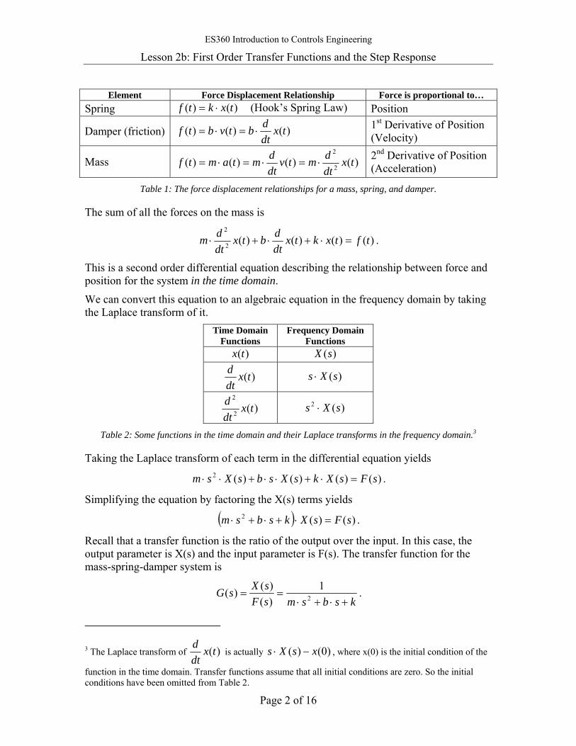
Element Force Displacement Relationship Force is proportional to…
Spring )()( txktf ⋅= (Hook’s Spring Law) Position
Damper (friction) )()()( txdtdbtvbtf ⋅=⋅= 1st Derivative of Position
(Velocity)
Mass )()()()( 2
2
txdtdmtv
dtdmtamtf ⋅=⋅=⋅= 2nd Derivative of Position
(Acceleration)
Table 1: The force displacement relationships for a mass, spring, and damper.
The sum of all the forces on the mass is
)()()()(2
2
tftxktxdtdbtx
dtdm =⋅+⋅+⋅ .
This is a second order differential equation describing the relationship between force and position for the system in the time domain.
We can convert this equation to an algebraic equation in the frequency domain by taking the Laplace transform of it.
Time Domain Functions
Frequency Domain Functions
)(tx )(sX
)(txdtd )(sXs ⋅
)(2
2
txdtd )(2 sXs ⋅
Table 2: Some functions in the time domain and their Laplace transforms in the frequency domain.3
Taking the Laplace transform of each term in the differential equation yields
)()()()(2 sFsXksXsbsXsm =⋅+⋅⋅+⋅⋅ .
Simplifying the equation by factoring the X(s) terms yields
( ) )()(2 sFsXksbsm =⋅+⋅+⋅ .
Recall that a transfer function is the ratio of the output over the input. In this case, the output parameter is X(s) and the input parameter is F(s). The transfer function for the mass-spring-damper system is
ksbsmsFsXsG
+⋅+⋅== 2
1)()()( .
3 The Laplace transform of )(txdtd
is actually )0()( xsXs −⋅ , where x(0) is the initial condition of the
function in the time domain. Transfer functions assume that all initial conditions are zero. So the initial conditions have been omitted from Table 2.

ES360 Introduction to Controls Engineering Lesson 2b: First Order Transfer Functions and the Step Response
Page 3 of 16
A System’s Order A system’s order is physically determined by the number of independent energy storage elements within the system. This corresponds to the highest power of s in the transfer function’s denominator. For example:
11+s
is a transfer function for a 1st order system with only a single energy storage element.
321
2 ++ ss
is a transfer function for a 2nd order system with two energy storage elements. And
2471
23 +++ sss
is a transfer functions for a 3rd order system with three energy storage elements.
ES360 Introduction to Controls Engineering Lesson 2b: First Order Transfer Functions and the Step Response
Page 4 of 16
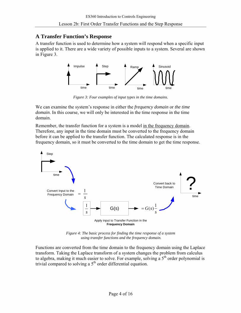
A Transfer Function’s Response A transfer function is used to determine how a system will respond when a specific input is applied to it. There are a wide variety of possible inputs to a system. Several are shown in Figure 3.
time
Step
time
Impulse
time
Ramp
time
Sinusoid
Figure 3: Four examples of input types in the time domains.
We can examine the system’s response in either the frequency domain or the time domain. In this course, we will only be interested in the time response in the time domain.
Remember, the transfer function for a system is a model in the frequency domain. Therefore, any input in the time domain must be converted to the frequency domain before it can be applied to the transfer function. The calculated response is in the frequency domain, so it must be converted to the time domain to get the time response.
time
Step
G(s)
Apply input to Transfer Function in theFrequency Domain
s1
ssG 1)(=
time
?Convert back toTime Domain
Convert Input to theFrequency Domain
s1
=
Figure 4: The basic process for finding the time response of a system
using transfer functions and the frequency domain.
Functions are converted from the time domain to the frequency domain using the Laplace transform. Taking the Laplace transform of a system changes the problem from calculus to algebra, making it much easier to solve. For example, solving a 5th order polynomial is trivial compared to solving a 5th order differential equation.
ES360 Introduction to Controls Engineering Lesson 2b: First Order Transfer Functions and the Step Response
Page 5 of 16
First Order Transfer Functions and the Step Response One of the simplest transfer functions is the first order transfer function. It has the general form
σ+=
sasG )( .
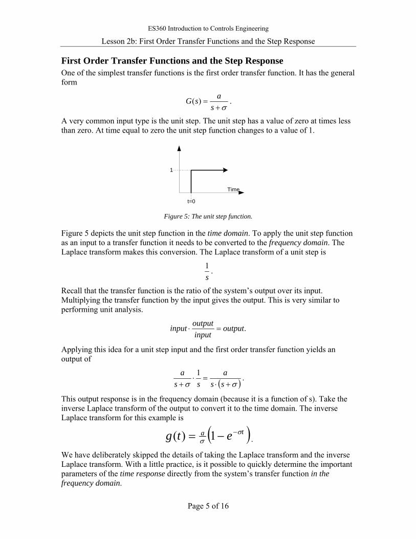
A very common input type is the unit step. The unit step has a value of zero at times less than zero. At time equal to zero the unit step function changes to a value of 1.
Time
t=0
1
Figure 5: The unit step function.
Figure 5 depicts the unit step function in the time domain. To apply the unit step function as an input to a transfer function it needs to be converted to the frequency domain. The Laplace transform makes this conversion. The Laplace transform of a unit step is
s1 .
Recall that the transfer function is the ratio of the system’s output over its input. Multiplying the transfer function by the input gives the output. This is very similar to performing unit analysis.
.outputinputoutputinput =⋅
Applying this idea for a unit step input and the first order transfer function yields an output of
( )σσ +⋅=⋅
+ ssa
ssa 1 .
This output response is in the frequency domain (because it is a function of s). Take the inverse Laplace transform of the output to convert it to the time domain. The inverse Laplace transform for this example is
( )ta etg σσ
−−= 1)( .
We have deliberately skipped the details of taking the Laplace transform and the inverse Laplace transform. With a little practice, is it possible to quickly determine the important parameters of the time response directly from the system’s transfer function in the frequency domain.

ES360 Introduction to Controls Engineering Lesson 2b: First Order Transfer Functions and the Step Response
Page 6 of 16
1) Sketch a plot of te−−1 on the axes below. Your calculator may be helpful.
time
All first order transfer functions have this shape as their step response!
2) Write the equation for the step response (in the time domain) for the following first order transfer functions. Label each curve on the plot with its corresponding transfer function. Your calculator may be helpful in correlating each curve with its transfer function.
Transfer Function (Frequency Domain)
Unit Step Response(Time Domain)
a 1
1+s
b 2
2+s
c 1
2+s
Step Response
Time (sec)
Ampl
itude
0 1 2 3 4 5 60
0.2
0.4
0.6
0.8
1
1.2
1.4
1.6
1.8
2

ES360 Introduction to Controls Engineering Lesson 2b: First Order Transfer Functions and the Step Response
Page 7 of 16
The step response of a first order system can be measured by two parameters.
• Settling Time: This is the length of time it takes the system to reach its final value.
• DC Gain: This is the value of the transfer function as frequency (s) approaches zero. Frequency approaching zero is equivalent to time approaching infinity. It is the ratio of the steady state output over the steady state input (the step magnitude).
Settling Time Mathematically the system approaches its final value asymptotically. Theoretically it never actually reaches the final value. For practical purposes, the system is considered at its final value when it is within 2% of the asymptotic value4.
Recall, the general form of the step response in the time domain is given by
( )ta etg σσ
−−= 1)( .
3) How are the values for DC gain and the settling time specified in this equation?
DC Gain: Settling Time:
In a first order transfer function σ1 is the time constant of the system. The value of σ
determines how quickly the system will approach its final value.
4a) Find the settling time (Ts) in terms of σ by solving the following equation for t. Show each step!
te σ−=%2
Ts =
Since these calculations are approximations of the system’s response, the answer above is rounded to
σ4
=sT
4b) After one time constant has elapsed, σ1=t , how close is a first order system to its
final value? Hint: Solve te σ−−1 .
Percent of System’s Final Value After One = Time Constant
4 The 2% tolerance is common for measuring the performance of mechanical systems. In electrical engineering the performance tolerance on the final value is often 0.7% percent.
ES360 Introduction to Controls Engineering Lesson 2b: First Order Transfer Functions and the Step Response
Page 8 of 16
DC Gain A DC signal has a frequency of zero. Gain means multiplication. A system’s DC gain is the value of the transfer function at a frequency (s) of zero. This is the value the transfer function multiplies the input by at a frequency of zero. Recall
TimeFrequency 1
= .
Frequency approaching zero is equivalent to time approaching infinity. This means the DC gain of a transfer function is also the amount the input will be multiplied by as time approaches infinity.
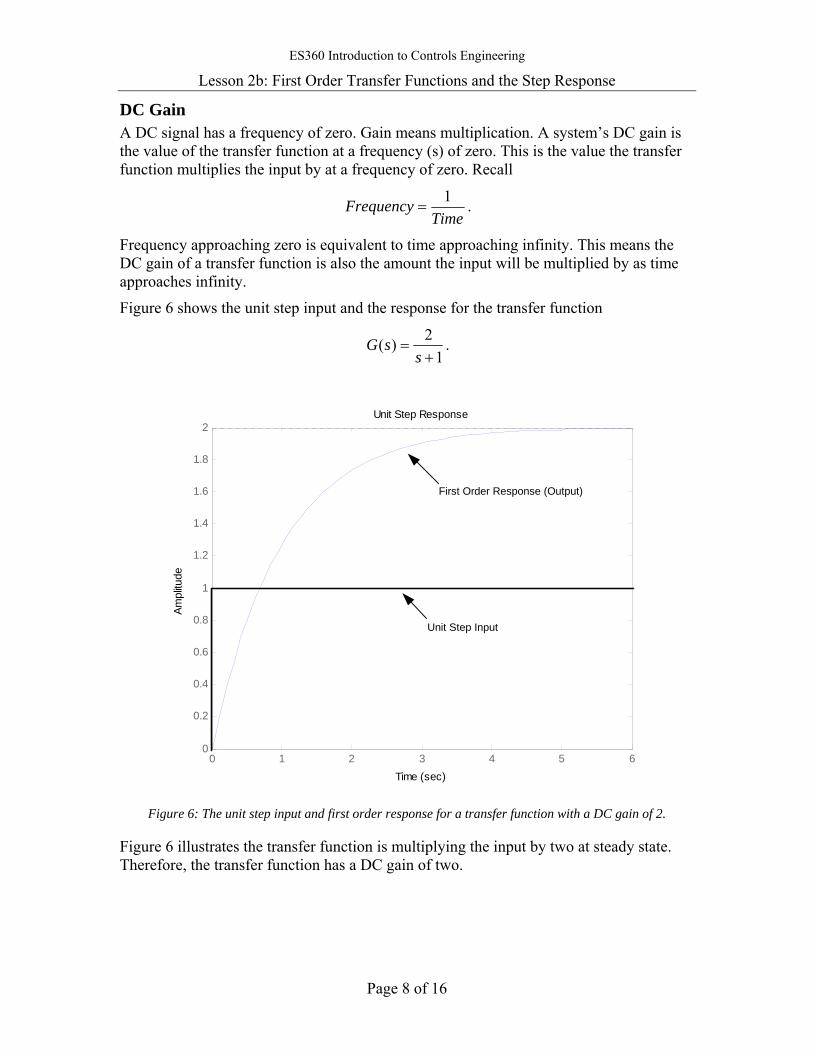
Figure 6 shows the unit step input and the response for the transfer function
12)(+
=s
sG .
0 1 2 3 4 5 60
0.2
0.4
0.6
0.8
1
1.2
1.4
1.6
1.8
2Unit Step Response
Time (sec)
Ampl
itude
Unit Step Input
First Order Response (Output)
Figure 6: The unit step input and first order response for a transfer function with a DC gain of 2.
Figure 6 illustrates the transfer function is multiplying the input by two at steady state. Therefore, the transfer function has a DC gain of two.
ES360 Introduction to Controls Engineering Lesson 2b: First Order Transfer Functions and the Step Response
Page 9 of 16
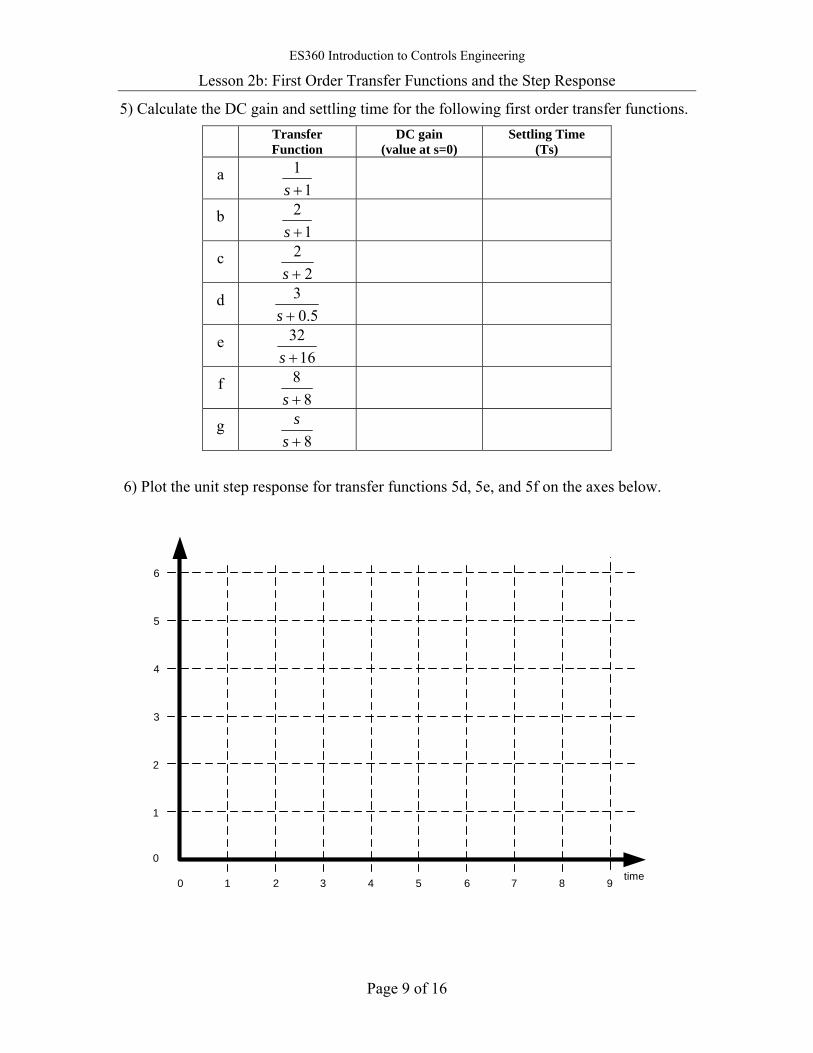
5) Calculate the DC gain and settling time for the following first order transfer functions.
Transfer Function
DC gain (value at s=0)
Settling Time (Ts)
a 1
1+s
b 1
2+s
c 2
2+s
d 5.0
3+s
e 16
32+s
f 8
8+s
g 8+s
s
6) Plot the unit step response for transfer functions 5d, 5e, and 5f on the axes below.
time
0
1
2
3
4
5
6
0 1 2 3 4 5 6 7 8 9
ES360 Introduction to Controls Engineering Lesson 2b: First Order Transfer Functions and the Step Response
Page 10 of 16
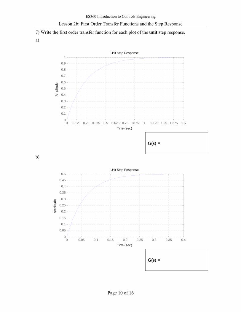
7) Write the first order transfer function for each plot of the unit step response.
a)
0 0.125 0.25 0.375 0.5 0.625 0.75 0.875 1 1.125 1.25 1.375 1.50
0.1
0.2
0.3
0.4
0.5
0.6
0.7
0.8
0.9
1Unit Step Response
Time (sec)
Ampl
itude
G(s) =
b)
0 0.05 0.1 0.15 0.2 0.25 0.3 0.35 0.40
0.05
0.1
0.15
0.2
0.25
0.3
0.35
0.4
0.45
0.5Unit Step Response
Time (sec)
Ampl
itude
G(s) =
ES360 Introduction to Controls Engineering Lesson 2b: First Order Transfer Functions and the Step Response
Page 11 of 16
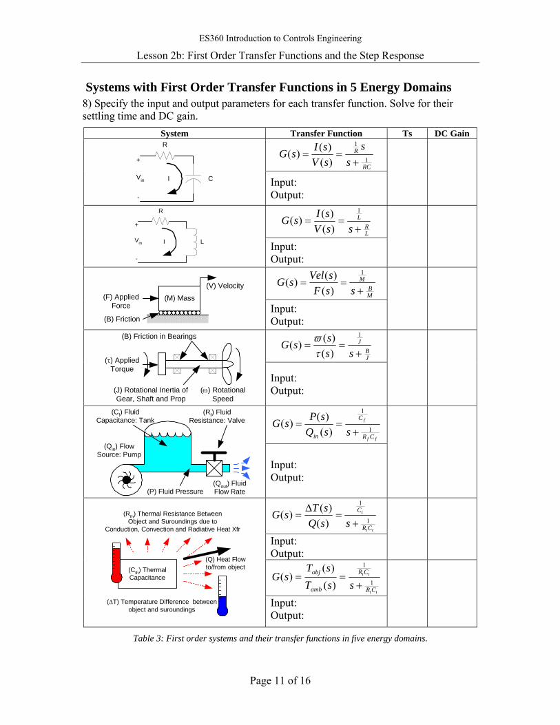
Systems with First Order Transfer Functions in 5 Energy Domains 8) Specify the input and output parameters for each transfer function. Solve for their settling time and DC gain.
System Transfer Function Ts DC Gain
RC
R
ss
sVsIsG
1
1
)()()(
+==
R
CVin I
+
-
Input: Output:
LR
L
ssVsIsG
+==
1
)()()(
R
LVin I
+
- Input: Output:
MB
M
ssFsVelsG
+==
1
)()()(
(M) Mass(F) AppliedForce
(B) Friction
(V) Velocity
Input: Output:
JB
J
ssssG
+==
1
)()()(
τϖ
(J) Rotational Inertia ofGear, Shaft and Prop
(B) Friction in Bearings
(τ) AppliedTorque
(ω) RotationalSpeed
Input: Output:
ff
f
CR
C
in ssQsPsG
1
1
)()()(
+==
(Qin) FlowSource: Pump
(Cf) FluidCapacitance: Tank
(Rf) FluidResistance: Valve
(Qout) FluidFlow Rate(P) Fluid Pressure
Input: Output:
tt
t
CR
C
ssQsTsG
1
1
)()()(
+=
∆=
Input: Output:
tt
tt
CR
CR
amb
obj
ssTsT
sG1
1
)()(
)(+
==(Cth) ThermalCapacitance
(Rth) Thermal Resistance BetweenObject and Suroundings due to
Conduction, Convection and Radiative Heat Xfr
(∆T) Temperature Difference betweenobject and suroundings
(Q) Heat Flowto/from object
Input: Output:
Table 3: First order systems and their transfer functions in five energy domains.
ES360 Introduction to Controls Engineering Lesson 2b: First Order Transfer Functions and the Step Response
Page 12 of 16
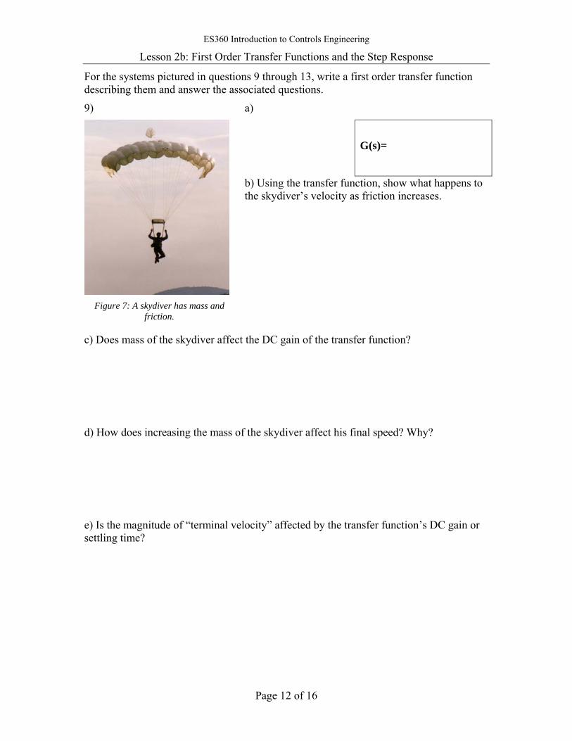
For the systems pictured in questions 9 through 13, write a first order transfer function describing them and answer the associated questions.
9)
Figure 7: A skydiver has mass and
friction.
a)
G(s)=
b) Using the transfer function, show what happens to the skydiver’s velocity as friction increases.
c) Does mass of the skydiver affect the DC gain of the transfer function?
d) How does increasing the mass of the skydiver affect his final speed? Why?
e) Is the magnitude of “terminal velocity” affected by the transfer function’s DC gain or settling time?

ES360 Introduction to Controls Engineering Lesson 2b: First Order Transfer Functions and the Step Response
Page 13 of 16
10) Reciprocating engines (like the one in a car or steam engine) produce varying amounts of torque. They produce the most torque when a cylinder is firing. When no cylinders are firing, no torque is generated. A flywheel is used to smooth out the rotary motion produced by the engine. The momentum of the flywheel keeps the engine rotating when a cylinder is not firing.
Flywheel Figure 8: Flywheels are used to smooth the output of external
(left) and internal (right) combustion engines.
a)
G(s)=
b) Which parameter in the transfer function determines how well the flywheel smoothes out the rotary motion of the engine? Does this parameter change the steady state speed of the engine (i.e. the DC gain of the transfer function)?
c) Is it desirable to have a long or short settling time for a flywheel? Why?
d) What are two methods of adjusting the settling time of the flywheel? Why is one of these methods undesirable in an engine?
ES360 Introduction to Controls Engineering Lesson 2b: First Order Transfer Functions and the Step Response
Page 14 of 16
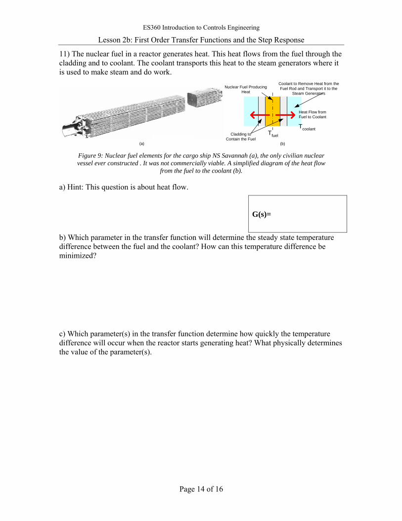
11) The nuclear fuel in a reactor generates heat. This heat flows from the fuel through the cladding and to coolant. The coolant transports this heat to the steam generators where it is used to make steam and do work.
(a)
Nuclear Fuel ProducingHeat
Cladding toContain the Fuel
Coolant to Remove Heat from theFuel Rod and Transport it to the
Steam Generators
Tfuel
Tcoolant
Heat Flow fromFuel to Coolant
(b) Figure 9: Nuclear fuel elements for the cargo ship NS Savannah (a), the only civilian nuclear vessel ever constructed . It was not commercially viable. A simplified diagram of the heat flow
from the fuel to the coolant (b).
a) Hint: This question is about heat flow.
G(s)=
b) Which parameter in the transfer function will determine the steady state temperature difference between the fuel and the coolant? How can this temperature difference be minimized?
c) Which parameter(s) in the transfer function determine how quickly the temperature difference will occur when the reactor starts generating heat? What physically determines the value of the parameter(s).

ES360 Introduction to Controls Engineering Lesson 2b: First Order Transfer Functions and the Step Response
Page 15 of 16
12) Large metal objects, like ships, take a significant amount of time to heat up and cool down. The environment around the ship will heat up and cool down much more quickly.
(a) (b) Figure 10: Thermal images of a ship several hours after sunset (a)
and of another ship several hours after sunrise (b).
Figure 10a shows a thermal image of a ship several hours after sunset. The ocean and atmosphere have cooled down faster than the ship. The ship will remain warmer than the environment for many hours after sunset. The thermal imaging system indicates this by displaying the ship as lighter than its surroundings.
Throughout the night, the ship’s temperature cools down to match the ambient temperature. Figure 10b shows a thermal image of a ship a few hours after sunrise. The environment has warmed up much faster than the ship. The thermal imaging system indicates this by displaying the ship as darker than its surroundings.
a) What type of ships are shown in Figures 10a and 10b?
Ship Type 10a: Ship Type 10b:
b) Write a first order transfer function which describes how the temperature of the ship responds to the changes in ambient temperature.
c) What is the ship’s temperature in steady state? How is this indicated by the transfer function?
d) How much heat is flowing to/from the ship if it is at ambient temperature?
e) Does increasing the thermal mass (capacity) of the ship change the settling time for the temperature of the ship? Why?
f) Does increasing the thermal resistance of the ship change the settling time for the temperature of the ship? Why?
f) Does the thermal resistance change the final temperature of the ship? Why?
G(s) =

ES360 Introduction to Controls Engineering Lesson 2b: First Order Transfer Functions and the Step Response
Page 16 of 16
13) Water towers are often used as a pressure source for municipal water systems. A pump supplies the water to keep them full.
Figure 11: A water tower provides a fluid reservoir at a pressure for the
town’s water system.
a)
G(s) =
b) In the municipal water system, what physically determines the two parameters of the system’s transfer function?
c) If the flow to the water tower is stopped, what happens to the pressure of the municipal water supply? Explain using the transfer function.
d) During commercial breaks in the Super Bowl the system pressure of the municipal water system will drop dramatically. Explain why in terms of the transfer function.
e) If water departments want to minimize the pressure drop during commercial breaks, which parameter of the system should they improve? Why can they not “improve” the other parameter?
ES360 Introduction to Controls Engineering
Lesson 3a: Input Types and the Final Value Theorem
Page 1 of 3
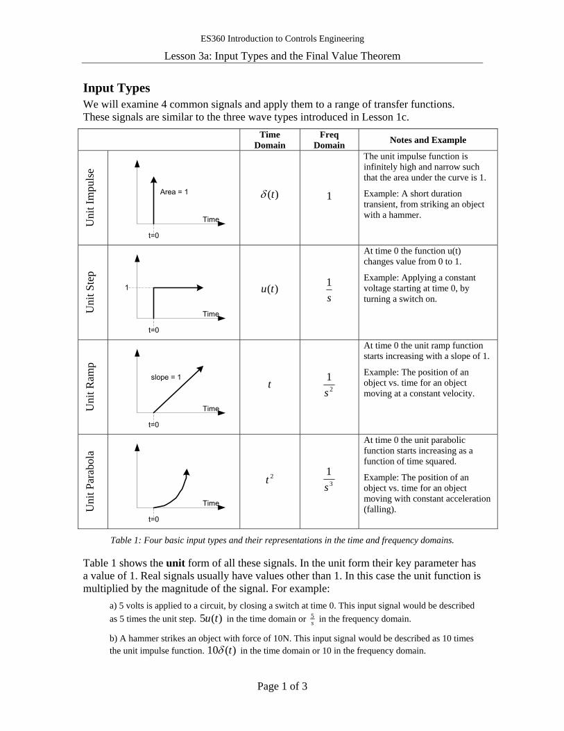
Input Types We will examine 4 common signals and apply them to a range of transfer functions. These signals are similar to the three wave types introduced in Lesson 1c.
Time Domain
Freq Domain Notes and Example
Uni
t Im
puls
e
Time
t=0
Area = 1 )(tδ 1
The unit impulse function is infinitely high and narrow such that the area under the curve is 1.
Example: A short duration transient, from striking an object with a hammer.
Uni
t Ste
p
Time
t=0
1 )(tu s1
At time 0 the function u(t) changes value from 0 to 1.
Example: Applying a constant voltage starting at time 0, by turning a switch on.
Uni
t Ram
p
Time
t=0
slope = 1t 2
1s
At time 0 the unit ramp function starts increasing with a slope of 1.
Example: The position of an object vs. time for an object moving at a constant velocity.
Uni
t Par
abol
a
Time
t=0
2t 3
1s
At time 0 the unit parabolic function starts increasing as a function of time squared.
Example: The position of an object vs. time for an object moving with constant acceleration (falling).
Table 1: Four basic input types and their representations in the time and frequency domains.
Table 1 shows the unit form of all these signals. In the unit form their key parameter has a value of 1. Real signals usually have values other than 1. In this case the unit function is multiplied by the magnitude of the signal. For example:
a) 5 volts is applied to a circuit, by closing a switch at time 0. This input signal would be described as 5 times the unit step. )(5 tu in the time domain or s
5 in the frequency domain.
b) A hammer strikes an object with force of 10N. This input signal would be described as 10 times the unit impulse function. )(10 tδ in the time domain or 10 in the frequency domain.
ES360 Introduction to Controls Engineering
Lesson 3a: Input Types and the Final Value Theorem
Page 2 of 3
The Final Value Theorem The final value theorem is a fast way of calculating the steady state value of a transfer function for a specific input. The final value theorem (FVT) states
)()(lim 0 sGsinputsValue seSteadyStat ⋅⋅= → .
Where G(s) is the transfer function and the input are specified in the frequency domain. Don’t forget the additional s term!
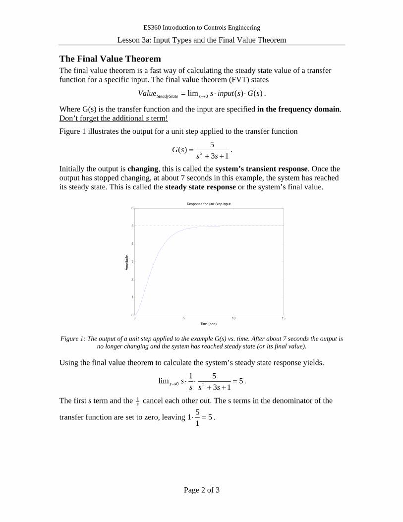
Figure 1 illustrates the output for a unit step applied to the transfer function
135)( 2 ++
=ss
sG .
Initially the output is changing, this is called the system’s transient response. Once the output has stopped changing, at about 7 seconds in this example, the system has reached its steady state. This is called the steady state response or the system’s final value.
Response for Unit Step Input
Time (sec)
Ampl
itude
0 5 10 150
1
2
3
4
5
6
Figure 1: The output of a unit step applied to the example G(s) vs. time. After about 7 seconds the output is
no longer changing and the system has reached steady state (or its final value).
Using the final value theorem to calculate the system’s steady state response yields.
513
51lim 20 =++
⋅⋅→ sssss .
The first s term and the s1 cancel each other out. The s terms in the denominator of the
transfer function are set to zero, leaving 5151 =⋅ .

ES360 Introduction to Controls Engineering
Lesson 3a: Input Types and the Final Value Theorem
Page 3 of 3
Final Value Theorem Exercise For each of the inputs and transfer functions below find the system’s steady state value using the final value theorem. Additionally, state the type of input being applied to the system or give its function in the frequency domain.
Input Transfer Function
TF’s DC Gain
Final Value
Input Type or Freq Domain
s1
224
2 ++ ss 2 2 unit step
unit ramp 32
32 ++ ss
1 ∞ 2
1s
a s5
315
2 ++ ss
b 2
4s
43
122 ++ ss
c unit step 32
62 ++ ss
d 5 32
62 ++ ss
e 2
1s
32
62 ++ ss
s
f 3
1s
32
212 ++ ss
g unit impulse 52
252 ++ ss
h 4 ss 5
352 +
i step of magnitude 5 432
1223 +++ sss
j impulse of magnitude 6 ss 5
52 +
k 3
25.0s
1
122
2
++ sss

ES360 Introduction to Controls Engineering
Lesson 3b: Second Order Systems’ Time Response
Page 1 of 9
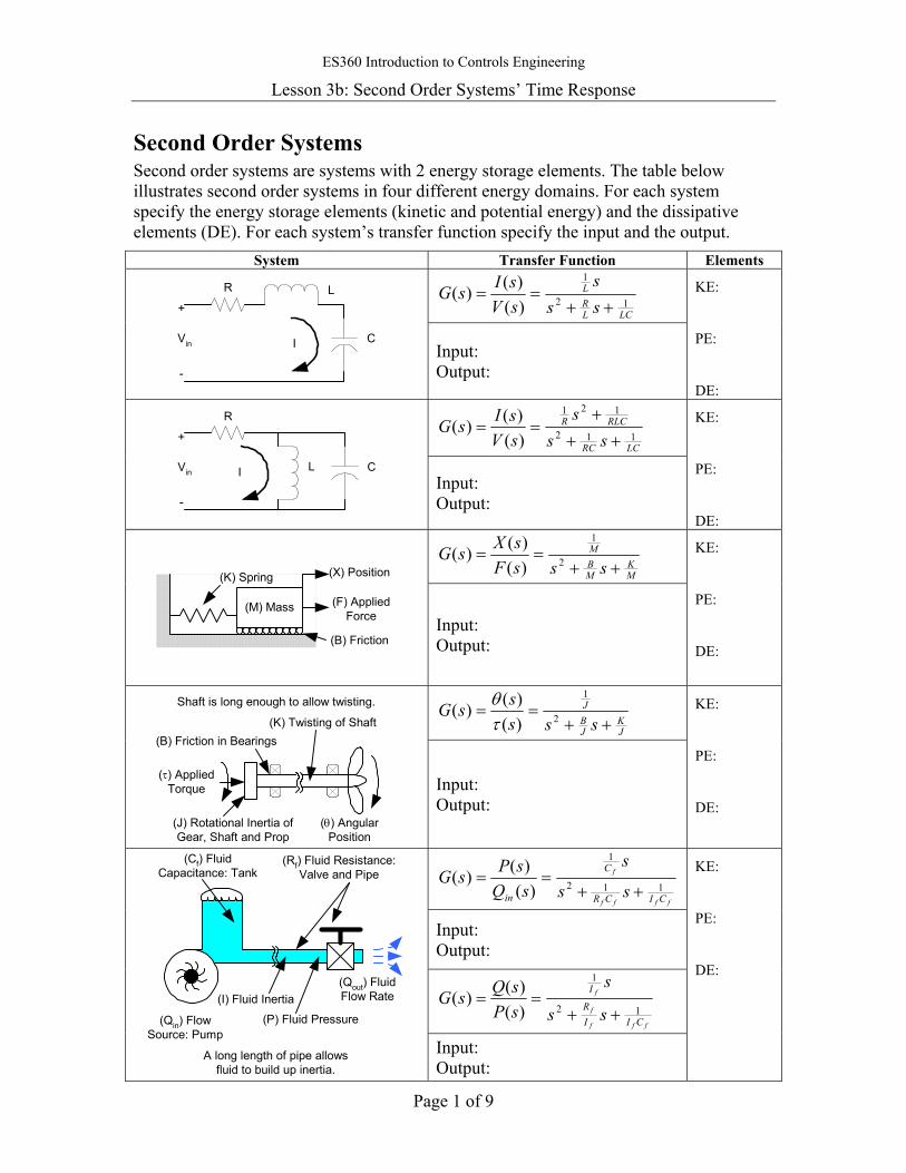
Second Order Systems Second order systems are systems with 2 energy storage elements. The table below illustrates second order systems in four different energy domains. For each system specify the energy storage elements (kinetic and potential energy) and the dissipative elements (DE). For each system’s transfer function specify the input and the output.
System Transfer Function Elements
LCLRL
sss
sVsIsG
12
1
)()()(
++== R
CVin I
+
-
L
Input: Output:
KE:
PE:
DE:
LCRC
RLCR
sss
sVsIsG
112
121
)()()(
+++
== R
CVin I
+
-
L
Input: Output:
KE:
PE:
DE:
MK
MBM
sssFsXsG
++== 2
1
)()()(
(M) Mass (F) AppliedForce
(B) Friction
(X) Position(K) Spring
Input: Output:
KE:
PE:
DE:
JK
JBJ
sssssG
++== 2
1
)()()(
τθ
(J) Rotational Inertia ofGear, Shaft and Prop
(B) Friction in Bearings
(τ) AppliedTorque
(θ) AngularPosition
(K) Twisting of Shaft
Shaft is long enough to allow twisting.
Input: Output:
KE:
PE:
DE:
ffff
f
CICR
C
in ss
s
sQsPsG
112
1
)()()(
++==
Input: Output:
fff
f
f
CIIR
I
ss
s
sPsQsG
12
1
)()()(
++==
(Qin) FlowSource: Pump
(Cf) FluidCapacitance: Tank
(Rf) Fluid Resistance:Valve and Pipe
(Qout) FluidFlow Rate
(P) Fluid Pressure
A long length of pipe allowsfluid to build up inertia.
(I) Fluid Inertia
Input: Output:
KE:
PE:
DE:
ES360 Introduction to Controls Engineering
Lesson 3b: Second Order Systems’ Time Response
Page 2 of 9
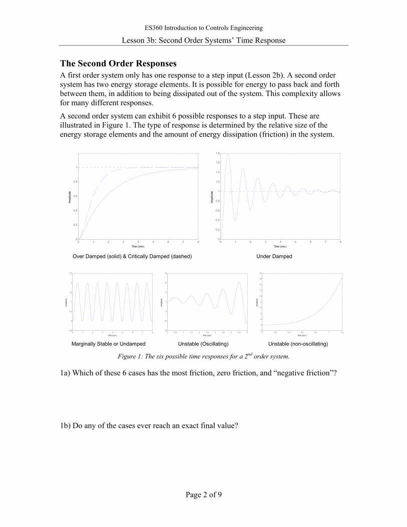
The Second Order Responses A first order system only has one response to a step input (Lesson 2b). A second order system has two energy storage elements. It is possible for energy to pass back and forth between them, in addition to being dissipated out of the system. This complexity allows for many different responses.
A second order system can exhibit 6 possible responses to a step input. These are illustrated in Figure 1. The type of response is determined by the relative size of the energy storage elements and the amount of energy dissipation (friction) in the system.
Time (sec)
Ampl
itude
0 1 2 3 4 5 6 7 8-0.5
0
0.5
1
1.5
2
2.5
Marginally Stable or Undamped
Time (sec)
Ampl
itude
0 0.5 1 1.5 2 2.5 3 3.5 4 4.5 5-15
-10
-5
0
5
10
15
Unstable (Oscillating)
Time (sec)
Ampl
itude
0 0.2 0.4 0.6 0.8 1 1.2-2
0
2
4
6
8
10
12
14
16
18
Unstable (non-oscillating)
Time (sec)
Ampl
itude
0 1 2 3 4 5 6 7 80
0.2
0.4
0.6
0.8
1
Over Damped (solid) & Critically Damped (dashed)
Time (sec)
Ampl
itude
0 1 2 3 4 5 6 7 80
0.2
0.4
0.6
0.8
1
1.2
1.4
1.6
1.8
Under Damped
Figure 1: The six possible time responses for a 2nd order system.
1a) Which of these 6 cases has the most friction, zero friction, and “negative friction”?
1b) Do any of the cases ever reach an exact final value?
ES360 Introduction to Controls Engineering
Lesson 3b: Second Order Systems’ Time Response
Page 3 of 9
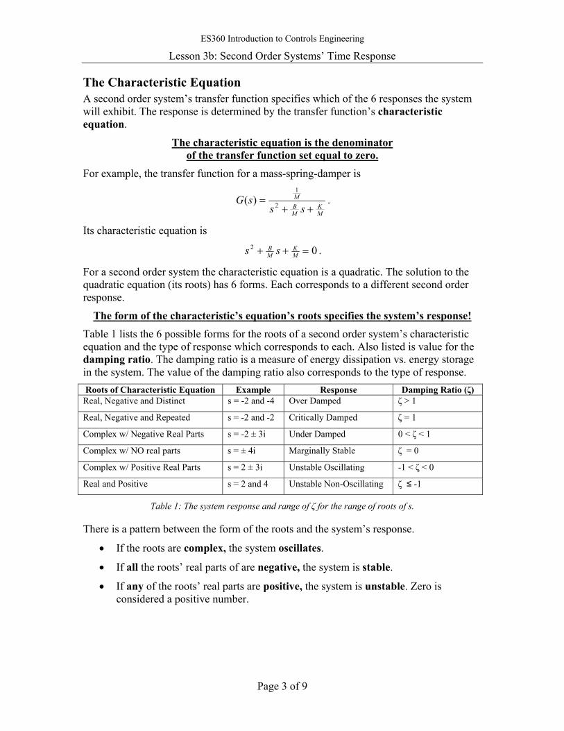
The Characteristic Equation A second order system’s transfer function specifies which of the 6 responses the system will exhibit. The response is determined by the transfer function’s characteristic equation.
The characteristic equation is the denominator of the transfer function set equal to zero.
For example, the transfer function for a mass-spring-damper is
MK
MBM
sssG
++= 2
1
)( .
Its characteristic equation is
02 =++ MK
MB ss .
For a second order system the characteristic equation is a quadratic. The solution to the quadratic equation (its roots) has 6 forms. Each corresponds to a different second order response.
The form of the characteristic’s equation’s roots specifies the system’s response!
Table 1 lists the 6 possible forms for the roots of a second order system’s characteristic equation and the type of response which corresponds to each. Also listed is value for the damping ratio. The damping ratio is a measure of energy dissipation vs. energy storage in the system. The value of the damping ratio also corresponds to the type of response. Roots of Characteristic Equation Example Response Damping Ratio (ζ) Real, Negative and Distinct s = -2 and -4 Over Damped ζ > 1
Real, Negative and Repeated s = -2 and -2 Critically Damped ζ = 1
Complex w/ Negative Real Parts s = -2 ± 3i Under Damped 0 < ζ < 1
Complex w/ NO real parts s = ± 4i Marginally Stable ζ = 0
Complex w/ Positive Real Parts s = 2 ± 3i Unstable Oscillating -1 < ζ < 0
Real and Positive s = 2 and 4 Unstable Non-Oscillating ζ ≤ -1
Table 1: The system response and range of ζ for the range of roots of s.
There is a pattern between the form of the roots and the system’s response.
• If the roots are complex, the system oscillates.
• If all the roots’ real parts of are negative, the system is stable.
• If any of the roots’ real parts are positive, the system is unstable. Zero is considered a positive number.

ES360 Introduction to Controls Engineering
Lesson 3b: Second Order Systems’ Time Response
Page 4 of 9
1c) Plot the roots of the characteristic equation which would give the response. Sketch the step response in the time domain. Give the value for the damping ratio.
Over Damped
ζ: σ
jω
Time
Critically Damped
ζ: σ
jω
Time
Under Damped
ζ: σ
jω
Time
Marginally Stable
ζ: σ
jω
Time
Unstable Oscillating
ζ: σ
jω
Time
Unstable Non-Oscillating
ζ: σ
jω
Time

ES360 Introduction to Controls Engineering
Lesson 3b: Second Order Systems’ Time Response
Page 5 of 9
Mass Spring Damper Example Consider the following simple mass spring damper system. With the following properties: M=10 kg, K=40 N/m, and B=20 Ns/m
(b)
t=0time
Applied Force f(t)
f=0
f=F
(a)
x(t)
f(t)
Mass (M)
Spring (K)
Damper (B)
Figure 2: The mass spring damper system (a) and the force applied to it as a function of time (b).
Figure 2a illustrates the mass spring damper system. From time zero onwards a constant force F is applied to the system as illustrated by Figure 2b. The system’s response (its motion) is measured by x(t).
2a) What kind of wave form is this force input (Lesson 1c)?
2b) With an applied force F of 100N, how far do you expect the mass to move (Hook’s Law)?
2c) Describe how the mass would move with no friction in the system (no damping). Make a sketch of x(t).
2d) Describe how the mass would move with a small amount of friction in the system. Make a sketch of x(t).
2e) Describe how the mass would move with a very large amount of friction in the system. Make a sketch of x(t).
xfinal =
time
x(t)
time
x(t)
time
x(t)
ES360 Introduction to Controls Engineering
Lesson 3b: Second Order Systems’ Time Response
Page 6 of 9
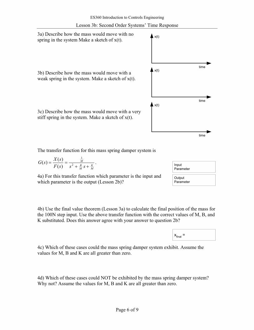
3a) Describe how the mass would move with no spring in the system Make a sketch of x(t).
3b) Describe how the mass would move with a weak spring in the system. Make a sketch of x(t).
3c) Describe how the mass would move with a very stiff spring in the system. Make a sketch of x(t).
The transfer function for this mass spring damper system is
MK
MBM
sssFsXsG
++== 2
1
)()()( .
4a) For this transfer function which parameter is the input and which parameter is the output (Lesson 2b)?
4b) Use the final value theorem (Lesson 3a) to calculate the final position of the mass for the 100N step input. Use the above transfer function with the correct values of M, B, and K substituted. Does this answer agree with your answer to question 2b?
4c) Which of these cases could the mass spring damper system exhibit. Assume the values for M, B and K are all greater than zero.
4d) Which of these cases could NOT be exhibited by the mass spring damper system? Why not? Assume the values for M, B and K are all greater than zero.
OutputParameter
InputParameter
time
x(t)
time
x(t)
time
x(t)
xfinal =
ES360 Introduction to Controls Engineering
Lesson 3b: Second Order Systems’ Time Response
Page 7 of 9
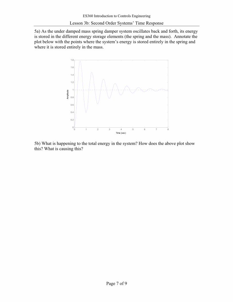
5a) As the under damped mass spring damper system oscillates back and forth, its energy is stored in the different energy storage elements (the spring and the mass). Annotate the plot below with the points where the system’s energy is stored entirely in the spring and where it is stored entirely in the mass.
Time (sec)
Ampl
itude
0 1 2 3 4 5 6 7 80
0.2
0.4
0.6
0.8
1
1.2
1.4
1.6
1.8
5b) What is happening to the total energy in the system? How does the above plot show this? What is causing this?

ES360 Introduction to Controls Engineering
Lesson 3b: Second Order Systems’ Time Response
Page 8 of 9
6) For each of the following transfer functions, find the characteristic equations, its roots, and its response type. J and K are tricky!
Transfer Function Characteristic
Equation Roots Response Type Name & Sketch
a 65
22 ++ ss
b 482
42 +− ss
c 1062
202 ++ ss
d 16
162 +s
e 2510
1002 ++ ss
f 82
82 +− ss
g 6.31210
25.42 ++ ss
h 1036
102 ++ ss
i 118
222 ++ ss
j ss 5
22 +
k 28
22 −+ ss

ES360 Introduction to Controls Engineering
Lesson 3b: Second Order Systems’ Time Response
Page 9 of 9
Using ltiview Next we will use MATLAB to test our predictions for the mass spring damper’s response. See the MATLAB help section of the workbook to learn how to enter transfer functions in MATLAB.
Write the system’s transfer function, substituting the values of M, B, and K into the transfer function.
7a) To display the system’s response to a unit step input, enter the transfer function into MATLAB and run the command ltiview(‘step’,G).1 What is the final displacement of the mass as displayed by MATLAB? Does this match your predictions in questions 2b and 10? Why or why not?
7b) Using ltiview answer questions 6 through 11 again.
• Print two plots. One plot with questions 2c, 2d, and 2e on the same graph, and another plot with questions 3a, 3b, and 3c on one graph.
• Label the curves with their question number and “high friction”, “low friction”, “no friction”, “strong spring”, “weak spring”, or “no spring” as appropriate.
Write the transfer function used for each curve below.
20) Which aspects of the time response were affected by changing the friction (B) and spring stiffness (K)?
1 Assuming the transfer function was saved in MATLAB as the variable “G”. If the variable was named something else, then use that name instead of “G”.
G(s) =
xfinal =
G2c(s) = G3a(s) =
G2d(s) = G3b(s) =
G2e(s) = G3c(s) =

ES360 Introduction to Controls Engineering
Lesson 4: Second Order Time Response Calculations
Page 1 of 8
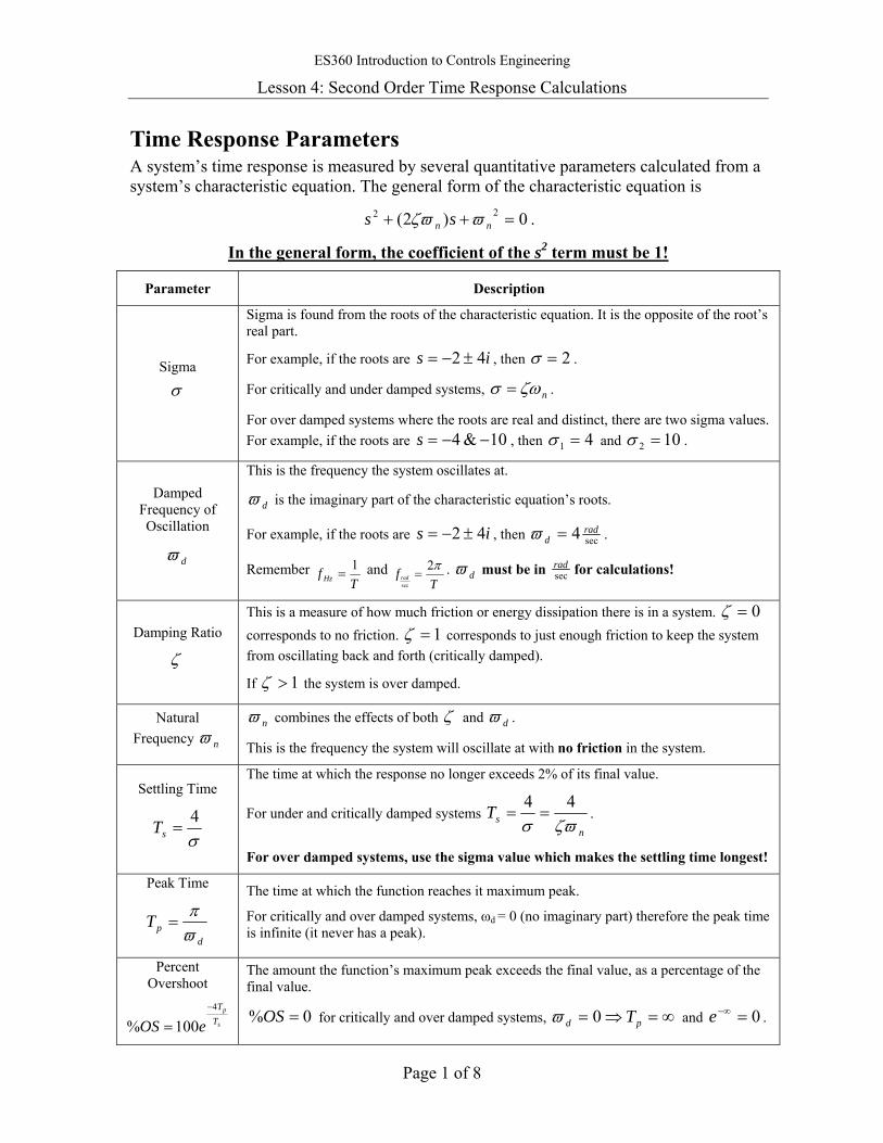
Time Response Parameters A system’s time response is measured by several quantitative parameters calculated from a system’s characteristic equation. The general form of the characteristic equation is
0)2( 22 =++ nn ss ϖζϖ .
In the general form, the coefficient of the s2 term must be 1!
Parameter Description
Sigma
σ
Sigma is found from the roots of the characteristic equation. It is the opposite of the root’s real part.
For example, if the roots are is 42 ±−= , then 2=σ .
For critically and under damped systems, nζωσ = .
For over damped systems where the roots are real and distinct, there are two sigma values. For example, if the roots are 10&4 −−=s , then 41 =σ and 102 =σ .
Damped Frequency of Oscillation
dϖ
This is the frequency the system oscillates at.
dϖ is the imaginary part of the characteristic equation’s roots.
For example, if the roots are is 42 ±−= , then sec4 radd =ϖ .
Remember T
f Hz1
= and T
f rad
π2sec
= . dϖ must be in secrad for calculations!
Damping Ratio
ζ
This is a measure of how much friction or energy dissipation there is in a system. 0=ζ corresponds to no friction. 1=ζ corresponds to just enough friction to keep the system from oscillating back and forth (critically damped).
If 1>ζ the system is over damped.
Natural Frequency nϖ
nϖ combines the effects of both ζ and dϖ .
This is the frequency the system will oscillate at with no friction in the system.
Settling Time
σ4
=sT
The time at which the response no longer exceeds 2% of its final value.
For under and critically damped systems n
sTζϖσ
44== .
For over damped systems, use the sigma value which makes the settling time longest!
Peak Time
dpT
ϖπ
=
The time at which the function reaches it maximum peak.
For critically and over damped systems, ωd = 0 (no imaginary part) therefore the peak time is infinite (it never has a peak).
Percent Overshoot
s
p
TT
eOS4
100%−
=
The amount the function’s maximum peak exceeds the final value, as a percentage of the final value.
0% =OS for critically and over damped systems, ∞=⇒= pd T0ϖ and 0=−∞e .
ES360 Introduction to Controls Engineering
Lesson 4: Second Order Time Response Calculations
Page 2 of 8
The Three Questions When analyzing a second order system there are three important questions.
1. Is the system stable? Use the roots of the characteristic equation to determine stability.
2. Is the system’s steady state value acceptable? Alternatively, how much is the error from the desired value? Use the final value theorem to determine if the system’s final value is adequate for the design or application.
3. Is the system’s transient response acceptable? There are several aspects of the system’s transient response which could make the response unacceptable:
a. Does the system get to its final value fast enough (settling time)?
b. Does the system overshoot its final value too much (%OS)?
c. Is the number of oscillations too many (ζ)?
d. Is the frequency of oscillation too high ( dω )?
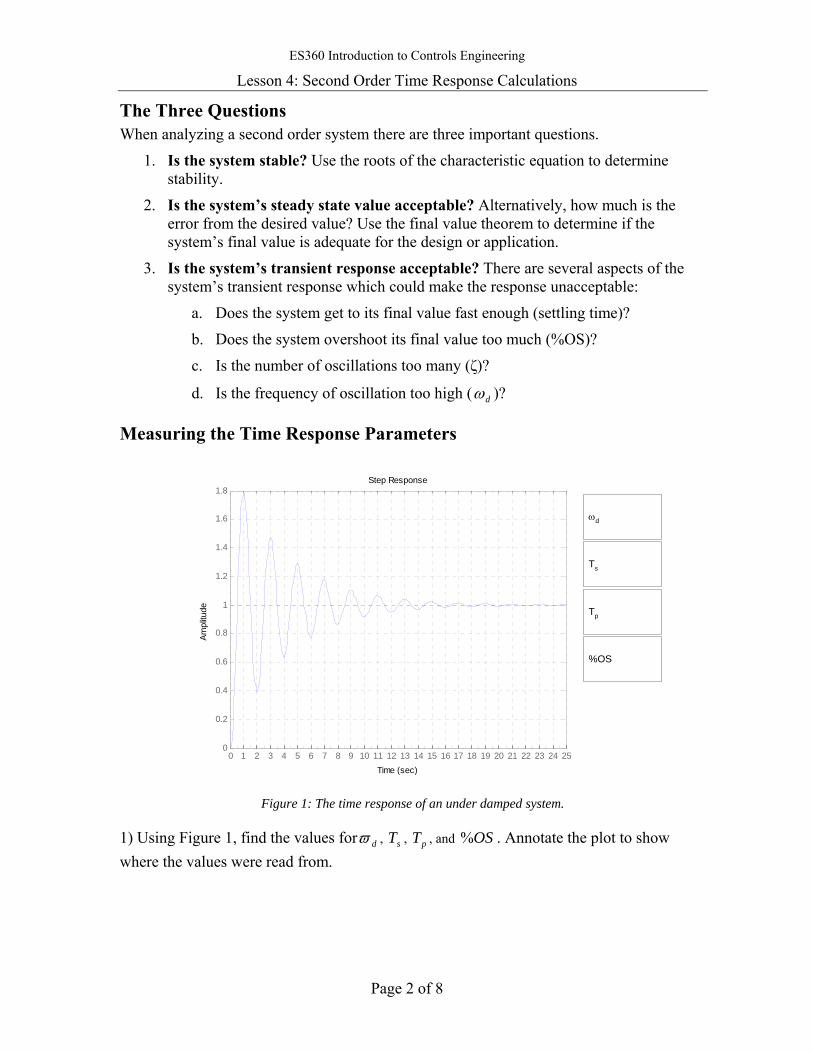
Measuring the Time Response Parameters
0 1 2 3 4 5 6 7 8 9 10 11 12 13 14 15 16 17 18 19 20 21 22 23 24 250
0.2
0.4
0.6
0.8
1
1.2
1.4
1.6
1.8Step Response
Time (sec)
Ampl
itude
ωd
Ts
Tp
%OS
Figure 1: The time response of an under damped system.
1) Using Figure 1, find the values for dϖ , sT , pT , and OS% . Annotate the plot to show where the values were read from.
ES360 Introduction to Controls Engineering
Lesson 4: Second Order Time Response Calculations
Page 3 of 8
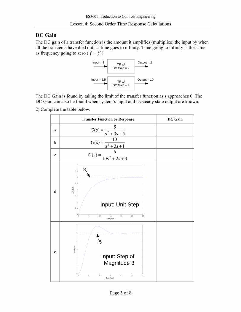
DC Gain The DC gain of a transfer function is the amount it amplifies (multiplies) the input by when all the transients have died out, as time goes to infinity. Time going to infinity is the same as frequency going to zero ( Tf 1= ).
TF w/DC Gain = 2
Input = 1 Output = 2
TF w/DC Gain = 4
Input = 2.5 Output = 10
The DC Gain is found by taking the limit of the transfer function as s approaches 0. The DC Gain can also be found when system’s input and its steady state output are known.
2) Complete the table below.
Transfer Function or Response DC Gain
a 53
5)( 2 ++=
sssG
b 13
10)( 2 ++=
sssG
c 3210
6)( 2 ++=
sssG
d
0 5 10 15 20 25 300
0.5
1
1.5
2
2.5
3
3.5
4
Time (sec)
Ampl
itude
Input: Unit Step
3
e
0 2 4 6 8 10 120
1
2
3
4
5
6
Time (sec)
Ampl
itude
Input: Step ofMagnitude 3
5
ES360 Introduction to Controls Engineering
Lesson 4: Second Order Time Response Calculations
Page 4 of 8
Calculating Time Response Parameters The system’s time response parameters can also be calculated directly from the characteristic equation for the transfer function.
Consider the transfer function
105.010)( 2 ++
=ss
sG .
3a) Write the transfer function’s characteristic equation.
Characteristic Eqn If the coefficient of the 2s term is one, then the terms of the characteristic equation map nicely to several time response parameters. The general form of the characteristic equation is
0)2( 22 =++ nn ss ϖζϖ .
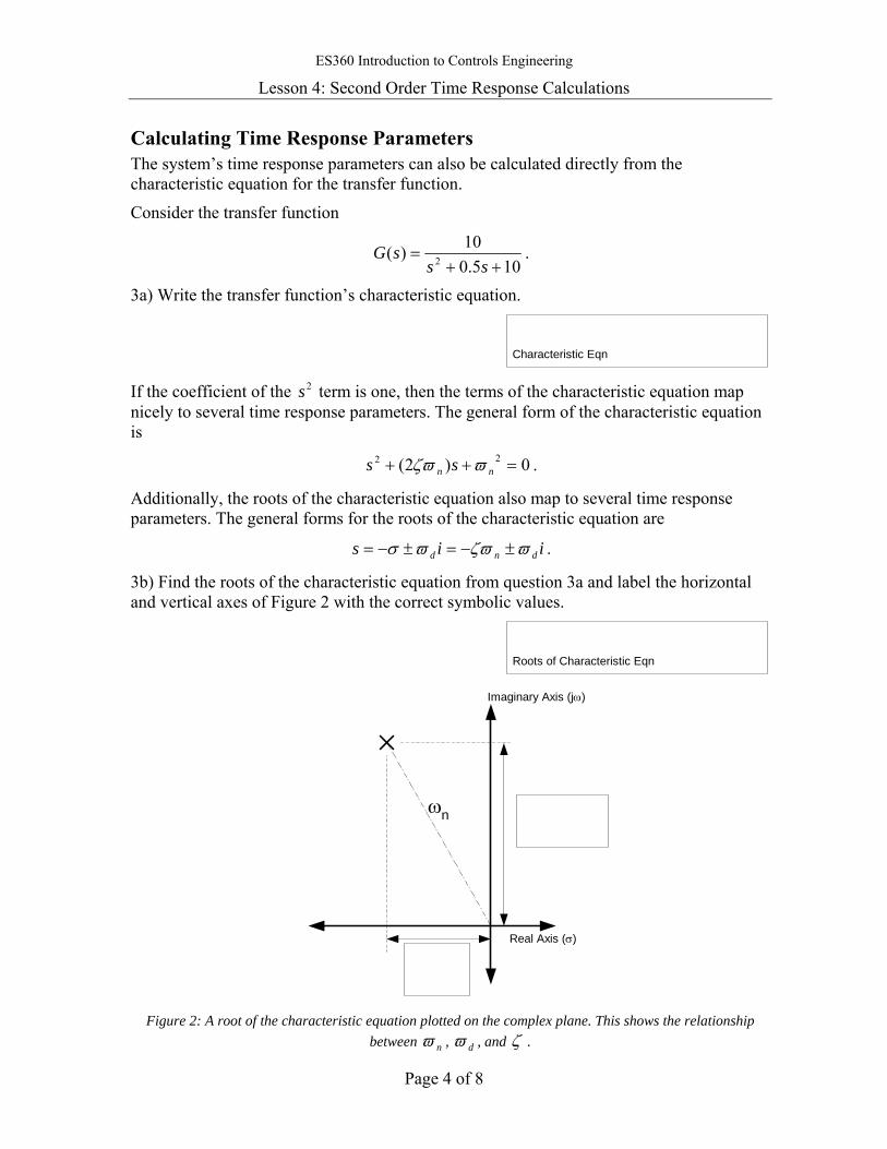
Additionally, the roots of the characteristic equation also map to several time response parameters. The general forms for the roots of the characteristic equation are
iis dnd ϖζϖϖσ ±−=±−= .
3b) Find the roots of the characteristic equation from question 3a and label the horizontal and vertical axes of Figure 2 with the correct symbolic values.
Roots of Characteristic Eqn
Real Axis (σ)
Imaginary Axis (jω)
ωn
Figure 2: A root of the characteristic equation plotted on the complex plane. This shows the relationship
between nϖ , dϖ , and ζ .
ES360 Introduction to Controls Engineering
Lesson 4: Second Order Time Response Calculations
Page 5 of 8
3c) Write an equation which describes the relationship between nϖ , dϖ , and ζ .
Eqn 3d) Calculate nϖ , dϖ , and ζ for the characteristic equation in question 3a. Calculating
nζϖ is often a useful intermediate step.
ωdωn ζζωn
After the parameters nϖ , dϖ , and ζ have been calculated, the remaining time response parameters are found with the equations:
σ4
=sT , d
pTϖπ
= , and s
p
TT
eOS4
100%−
= .
Remember, when calculating settling times for over damped systems, use the σ which gives the longest settling time!
3e) Find the settling time, peak time, and percent overshoot for this system.
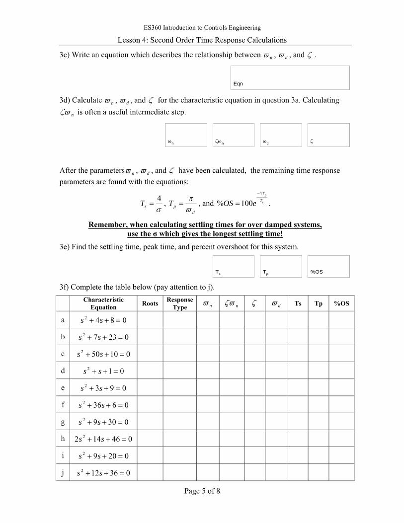
Ts Tp %OS 3f) Complete the table below (pay attention to j).
Characteristic Equation Roots Response
Type nϖ nζϖ ζ dϖ Ts Tp %OS
a 0842 =++ ss
b 02372 =++ ss
c 010502 =++ ss
d 012 =++ ss
e 0932 =++ ss
f 06362 =++ ss
g 03092 =++ ss
h 046142 2 =++ ss
i 02092 =++ ss
j 036122 =++ ss
ES360 Introduction to Controls Engineering
Lesson 4: Second Order Time Response Calculations
Page 6 of 8
4a) Using a sketch of the complex plane, explain why the natural frequency is the frequency the system oscillates at when the there is no friction.
Hint: What is the value of ζ when there is no friction.
4b) For the transfer function G(s) explain how increasing b, c, and d will affect the time response parameters.
Hint: A sketch of the complex plane will be useful.
csbsdsG
+⋅+= 2)(
Parameter ωn ζωn ζ ωd Ts Tp %OS DC Gain
b↑
c↑
d↑

ES360 Introduction to Controls Engineering
Lesson 4: Second Order Time Response Calculations
Page 7 of 8
5) Answer the following questions about the RLC circuit pictured below. R
CVin I
+
-
L
a) Write a transfer function for this system with voltage as the input and current as the output.
b) If a step input of 10 volts is applied to system what is the steady state current? Explain physically why this happens.
c) If the resistor has a value of 6 Ohms and the Inductor is 1mH, how big should the capacitor be to make the system critically damped?
d) As the value of the resistor increases explain what happens to each of the time response parameters.
Parameter ωn ζωn ζ ωd Ts Tp %OS DC Gain
R↑

ES360 Introduction to Controls Engineering
Lesson 4: Second Order Time Response Calculations
Page 8 of 8
6) Answer the following questions about the recoil mechanism of the Beretta M9 Pistol.
a) Write a transfer function for this system describing the recoil mechanism’s position for an applied force.
b) Label the components in the photos above which contribute to each parameter in the transfer function.
d) As the stiffness of the spring decreases explain what happens to each of the time response parameters.
Parameter ωn ζωn ζ ωd Ts Tp %OS DC Gain
ES360 Introduction to Controls Engineering
Lesson 5a: Graphical Analysis of Second Order Responses
Page 1 of 8
Graphical Analysis of Second Order Responses Transfer functions can be estimated for a system without knowing the internal configuration of the system. All that is required is to measure the system’s output as a response to a known input. With this information it is possible to solve for the system’s transfer function. This is a powerful and useful concept, particularly when modeling actual hardware.
First Order Review The concept of deriving a transfer function from a response was introduced for first order systems in Lesson 2b. Recall that the transfer function for a first order system is
σ+=
sasG )( .
Three steps are required to find a first order transfer from a system’s step response.
1. Solve for σ by either:
a) Find the time the response is at 63% of its final value. This time is the time constant σ1 . Solve for σ.
or b) Find the settling time for the system (the response is at 98% of its steady state
value1). Use σ4
=Ts to solve for σ .
Method 1a is usually a more accurate way of determining σ.
2. Divide the system’s steady state value by the magnitude of the step input to find its DC gain. A unit step has a magnitude of 1.
3. The DC gain is the value of the transfer function as s approaches zero. Use the DC gain and σ to solve for the numerator of the transfer function.
σσσ gainsgain DCaa
saDC =⇒=+
= →0lim
1 The system is considered to be at steady state when it is within 2% of its final value (98% of the system’s steady state value).
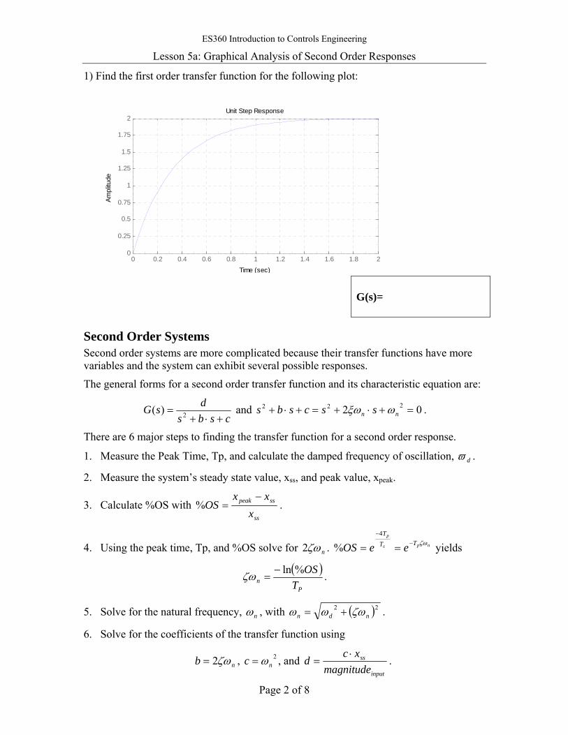
ES360 Introduction to Controls Engineering
Lesson 5a: Graphical Analysis of Second Order Responses
Page 2 of 8
1) Find the first order transfer function for the following plot:
0 0.2 0.4 0.6 0.8 1 1.2 1.4 1.6 1.8 20
0.25
0.5
0.75
1
1.25
1.5
1.75
2Unit Step Response
Time (sec)
Ampl
itude
G(s)=
Second Order Systems Second order systems are more complicated because their transfer functions have more variables and the system can exhibit several possible responses.
The general forms for a second order transfer function and its characteristic equation are:
csbsdsG
+⋅+= 2)( and 02 222 =+⋅+=+⋅+ nn sscsbs ωξω .
There are 6 major steps to finding the transfer function for a second order response.
1. Measure the Peak Time, Tp, and calculate the damped frequency of oscillation, dϖ .
2. Measure the system’s steady state value, xss, and peak value, xpeak.
3. Calculate %OS with ss
sspeak
xxx
OS−
=% .
4. Using the peak time, Tp, and %OS solve for nζω2 . nps
p
TTT
eeOS ζω−−
==4
% yields
( )P
n TOS%ln−
=ζω .
5. Solve for the natural frequency, nω , with ( )22ndn ζωωω += .
6. Solve for the coefficients of the transfer function using
nb ζω2= , 2nc ω= , and
input
ss
magnitudexc
d⋅
= .
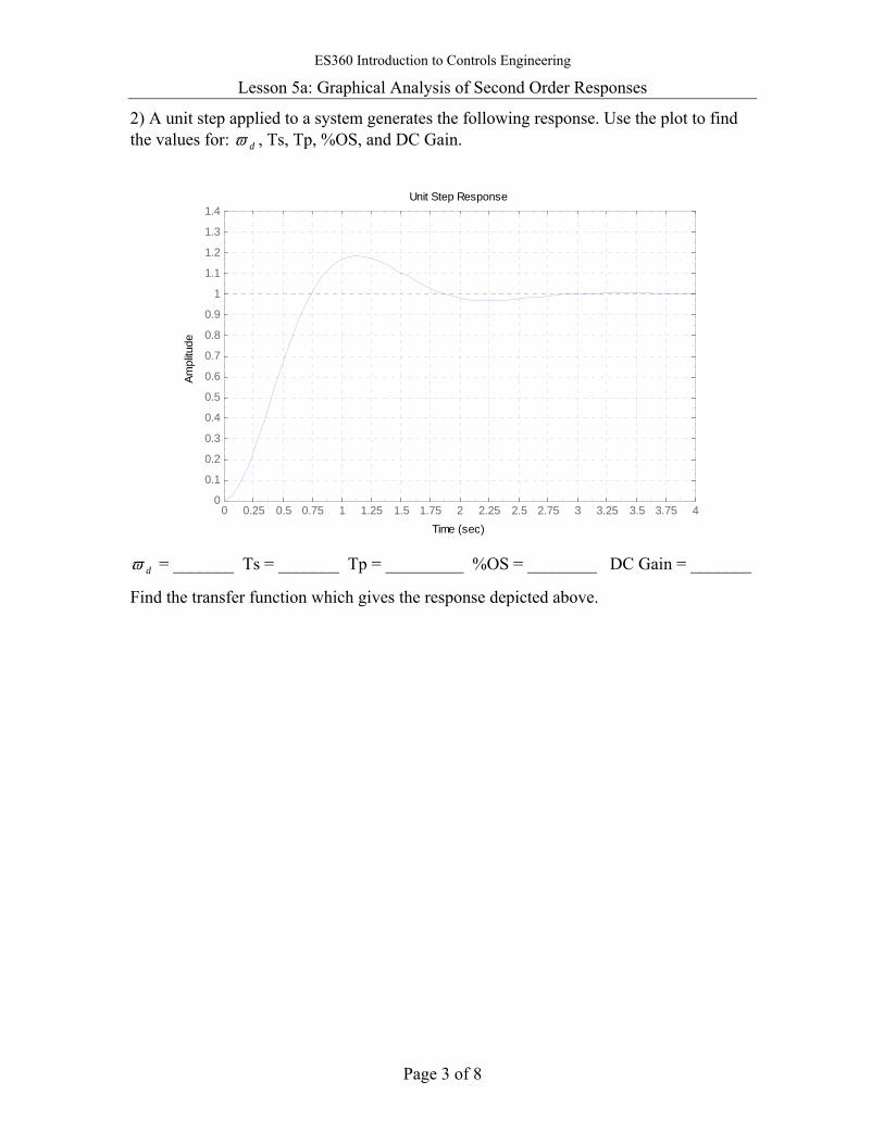
ES360 Introduction to Controls Engineering
Lesson 5a: Graphical Analysis of Second Order Responses
Page 3 of 8
2) A unit step applied to a system generates the following response. Use the plot to find the values for: dϖ , Ts, Tp, %OS, and DC Gain.
0 0.25 0.5 0.75 1 1.25 1.5 1.75 2 2.25 2.5 2.75 3 3.25 3.5 3.75 40
0.1
0.2
0.3
0.4
0.5
0.6
0.7
0.8
0.9
1
1.1
1.2
1.3
1.4Unit Step Response
Time (sec)
Ampl
itude
dϖ = _______ Ts = _______ Tp = _________ %OS = ________ DC Gain = _______
Find the transfer function which gives the response depicted above.
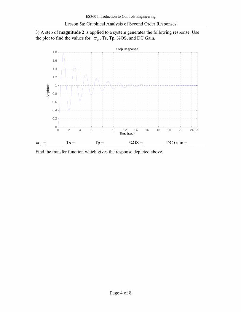
ES360 Introduction to Controls Engineering
Lesson 5a: Graphical Analysis of Second Order Responses
Page 4 of 8
3) A step of magnitude 2 is applied to a system generates the following response. Use the plot to find the values for: dϖ , Ts, Tp, %OS, and DC Gain.
Step Response
Time (sec)
Ampl
itude
0 2 4 6 8 10 12 14 16 18 20 22 24 250
0.2
0.4
0.6
0.8
1
1.2
1.4
1.6
1.8
dϖ = _______ Ts = _______ Tp = _________ %OS = ________ DC Gain = _______
Find the transfer function which gives the response depicted above.
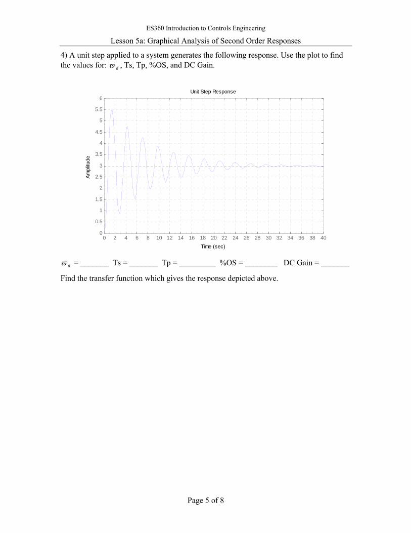
ES360 Introduction to Controls Engineering
Lesson 5a: Graphical Analysis of Second Order Responses
Page 5 of 8
4) A unit step applied to a system generates the following response. Use the plot to find the values for: dϖ , Ts, Tp, %OS, and DC Gain.
0 2 4 6 8 10 12 14 16 18 20 22 24 26 28 30 32 34 36 38 400
0.5
1
1.5
2
2.5
3
3.5
4
4.5
5
5.5
6Unit Step Response
Time (sec)
Ampl
itude
dϖ = _______ Ts = _______ Tp = _________ %OS = ________ DC Gain = _______
Find the transfer function which gives the response depicted above.
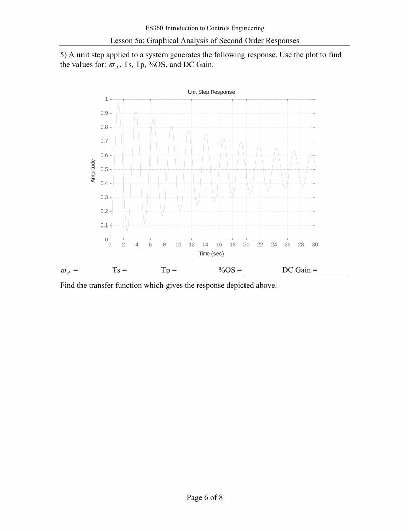
ES360 Introduction to Controls Engineering
Lesson 5a: Graphical Analysis of Second Order Responses
Page 6 of 8
5) A unit step applied to a system generates the following response. Use the plot to find the values for: dϖ , Ts, Tp, %OS, and DC Gain.
0 2 4 6 8 10 12 14 16 18 20 22 24 26 28 300
0.1
0.2
0.3
0.4
0.5
0.6
0.7
0.8
0.9
1Unit Step Response
Time (sec)
Ampl
itude
dϖ = _______ Ts = _______ Tp = _________ %OS = ________ DC Gain = _______
Find the transfer function which gives the response depicted above.
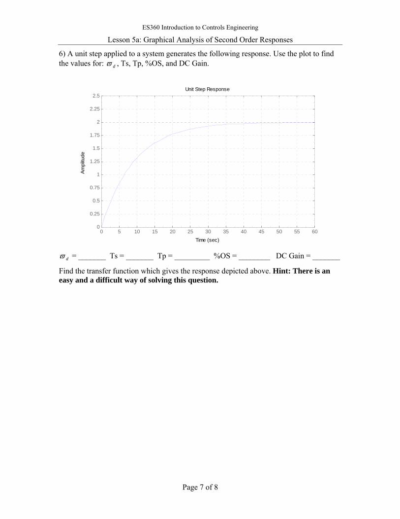
ES360 Introduction to Controls Engineering
Lesson 5a: Graphical Analysis of Second Order Responses
Page 7 of 8
6) A unit step applied to a system generates the following response. Use the plot to find the values for: dϖ , Ts, Tp, %OS, and DC Gain.
0 5 10 15 20 25 30 35 40 45 50 55 600
0.25
0.5
0.75
1
1.25
1.5
1.75
2
2.25
2.5Unit Step Response
Time (sec)
Ampl
itude
dϖ = _______ Ts = _______ Tp = _________ %OS = ________ DC Gain = _______
Find the transfer function which gives the response depicted above. Hint: There is an easy and a difficult way of solving this question.
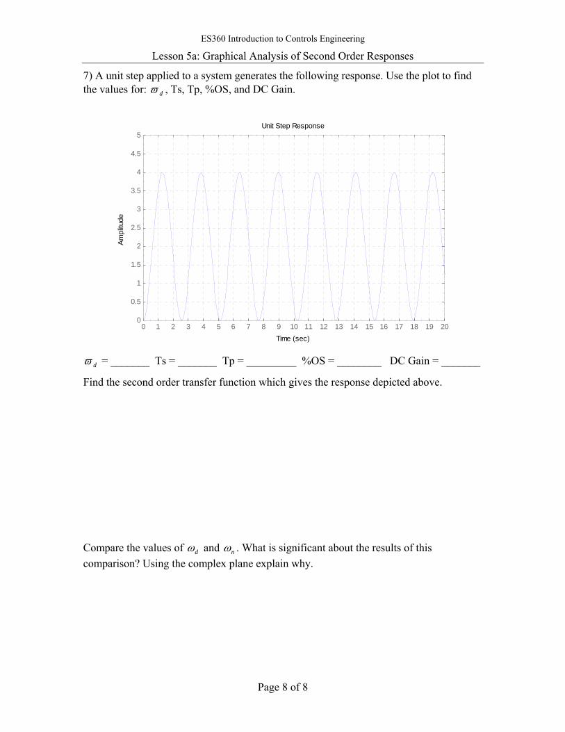
ES360 Introduction to Controls Engineering
Lesson 5a: Graphical Analysis of Second Order Responses
Page 8 of 8
7) A unit step applied to a system generates the following response. Use the plot to find the values for: dϖ , Ts, Tp, %OS, and DC Gain.
0 1 2 3 4 5 6 7 8 9 10 11 12 13 14 15 16 17 18 19 200
0.5
1
1.5
2
2.5
3
3.5
4
4.5
5Unit Step Response
Time (sec)
Ampl
itude
dϖ = _______ Ts = _______ Tp = _________ %OS = ________ DC Gain = _______
Find the second order transfer function which gives the response depicted above.
Compare the values of dω and nω . What is significant about the results of this comparison? Using the complex plane explain why.
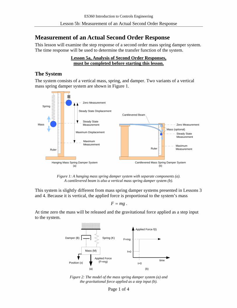
ES360 Introduction to Controls Engineering
Lesson 5b: Measurement of an Actual Second Order Response
Page 1 of 4
Measurement of an Actual Second Order Response This lesson will examine the step response of a second order mass spring damper system. The time response will be used to determine the transfer function of the system.
Lesson 5a, Analysis of Second Order Responses, must be completed before starting this lesson.
The System The system consists of a vertical mass, spring, and damper. Two variants of a vertical mass spring damper system are shown in Figure 1.
Hanging Mass Spring Damper System(a)
Cantilevered Beam
Mass (optional)
Ruler
Zero Measurement
Steady StateMeasurement
MaximumMeasurement
Mass
Spring
Ruler
Zero Measurement
MaximumMeasurement
Steady StateMeasurement
Steady State Displacement
Maximum Displacement
Cantilevered Mass Spring Damper System(b)
Figure 1: A hanging mass spring damper system with separate components (a). A cantilevered beam is also a vertical mass spring damper system (b).
This system is slightly different from mass spring damper systems presented in Lessons 3 and 4. Because it is vertical, the applied force is proportional to the system’s mass
mgF = .
At time zero the mass will be released and the gravitational force applied as a step input to the system.
(b)
t=0time
Applied Force f(t)
f=0
F=mg
(a)
Spring (K)Damper (B)
Mass (M)
Applied Force(F=mg)Position (x)
Figure 2: The model of the mass spring damper system (a) and
the gravitational force applied as a step input (b).
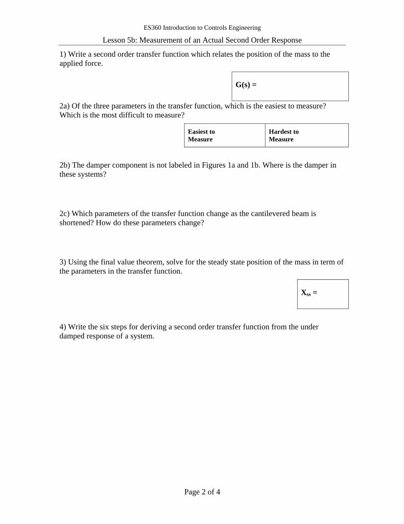
ES360 Introduction to Controls Engineering
Lesson 5b: Measurement of an Actual Second Order Response
Page 2 of 4
1) Write a second order transfer function which relates the position of the mass to the applied force.
G(s) =
2a) Of the three parameters in the transfer function, which is the easiest to measure? Which is the most difficult to measure?
Easiest to Measure
Hardest to Measure
2b) The damper component is not labeled in Figures 1a and 1b. Where is the damper in these systems?
2c) Which parameters of the transfer function change as the cantilevered beam is shortened? How do these parameters change?
3) Using the final value theorem, solve for the steady state position of the mass in term of the parameters in the transfer function.
Xss =
4) Write the six steps for deriving a second order transfer function from the under damped response of a system.

ES360 Introduction to Controls Engineering
Lesson 5b: Measurement of an Actual Second Order Response
Page 3 of 4
This lesson can be accomplished with either the hanging mass spring damper shown in Figure 1a or the cantilevered beam shown in Figure 1b.
All calculations should be done in metric units1.
5) Measure or calculate the following:
Lab Setup (Circle One): Hanging Mass Cantilevered Beam
Line Parameter English Metric Notes
1 Gravity g m/s2 9.8
2 Mass M kg
3 Zero Measurement in m
4 Steady State Measurement in m
5 Steady State Displacement Xss in m line 4 - line 3
6 Spring Constant K N/m
7 Cantilevered Beam Length L m Cant. Beam Only
Release the mass from the zero measurement point and record the peak time, period of oscillation, and maximum displacement. Perform four trials and average the results.
It is easiest to have a single person dedicated to measuring each parameter (Tp, period of oscillation, and maximum measurement).
Trial Period of Oscillation Peak Time Maximum Measurement
1
2
3
4
Average
6a) From the average maximum measurement calculate the average maximum displacement, see Figure 1. Calculate the %OS for the system.
Average Maximum Displacement Average %OS
1 1 inch = 2.54 cm = 0.0254 m 1 lb = 0.453 kg = 453 grams
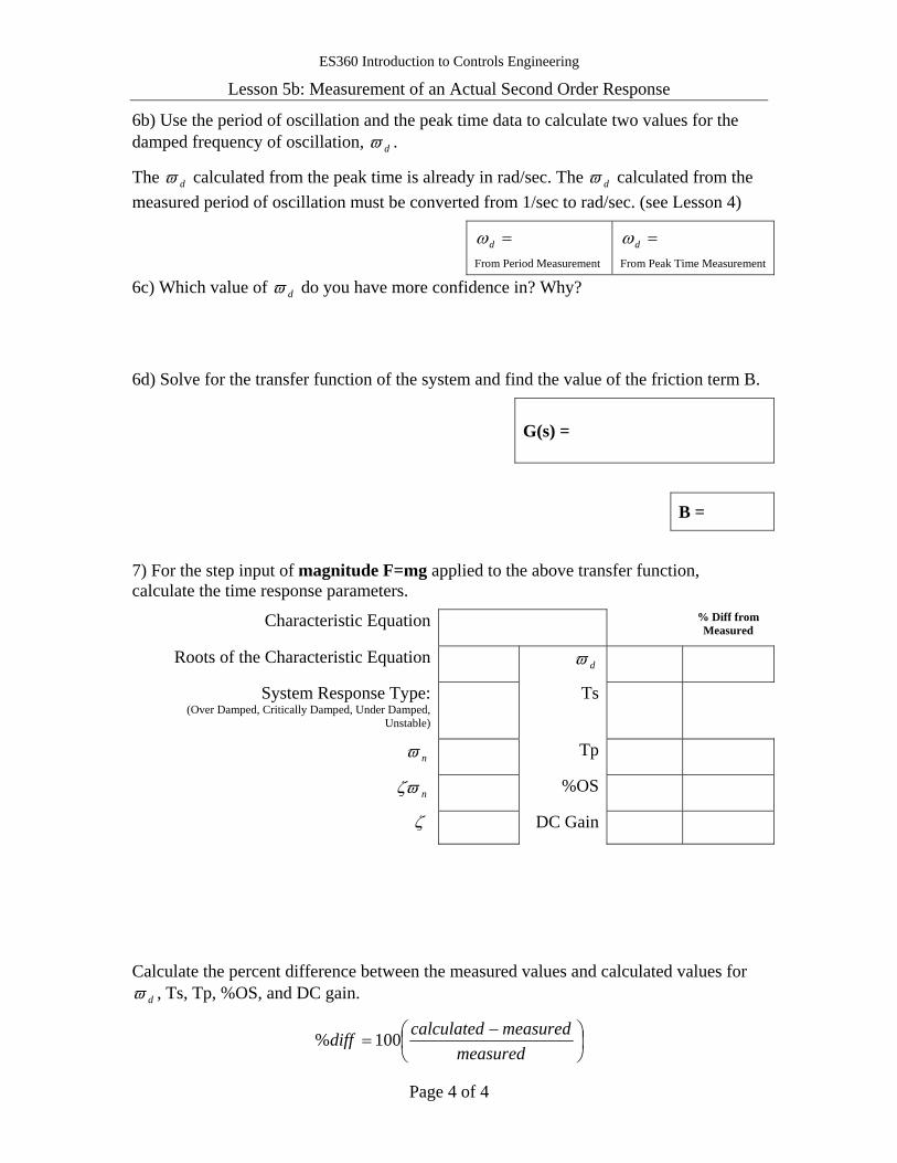
ES360 Introduction to Controls Engineering
Lesson 5b: Measurement of an Actual Second Order Response
Page 4 of 4
6b) Use the period of oscillation and the peak time data to calculate two values for the damped frequency of oscillation, dϖ .
The dϖ calculated from the peak time is already in rad/sec. The dϖ calculated from the measured period of oscillation must be converted from 1/sec to rad/sec. (see Lesson 4)
=dω
From Period Measurement
=dω
From Peak Time Measurement
6c) Which value of dϖ do you have more confidence in? Why?
6d) Solve for the transfer function of the system and find the value of the friction term B.
G(s) =
B =
7) For the step input of magnitude F=mg applied to the above transfer function, calculate the time response parameters.
Characteristic Equation % Diff from Measured
Roots of the Characteristic Equation dϖ
System Response Type:(Over Damped, Critically Damped, Under Damped,
Unstable)
Ts
nϖ Tp
nζϖ %OS
ζ DC Gain
Calculate the percent difference between the measured values and calculated values for dϖ , Ts, Tp, %OS, and DC gain.
⎟⎠⎞
⎜⎝⎛ −
=measured
measuredcalculateddiff 100%
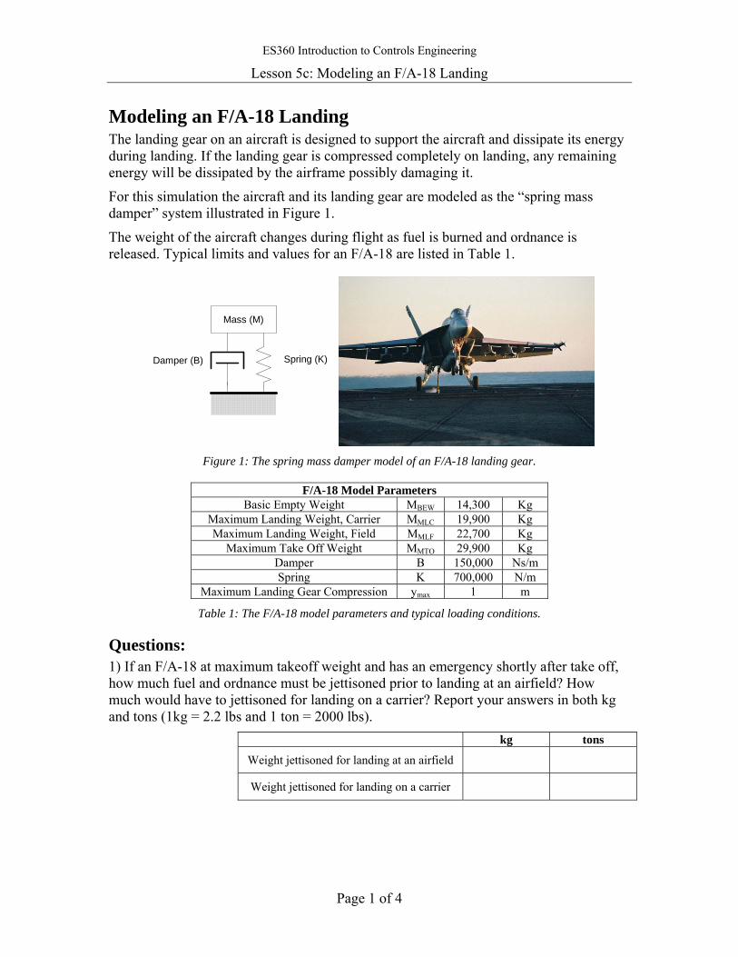
ES360 Introduction to Controls Engineering
Lesson 5c: Modeling an F/A-18 Landing
Page 1 of 4
Modeling an F/A-18 Landing The landing gear on an aircraft is designed to support the aircraft and dissipate its energy during landing. If the landing gear is compressed completely on landing, any remaining energy will be dissipated by the airframe possibly damaging it.
For this simulation the aircraft and its landing gear are modeled as the “spring mass damper” system illustrated in Figure 1.
The weight of the aircraft changes during flight as fuel is burned and ordnance is released. Typical limits and values for an F/A-18 are listed in Table 1.
Spring (K)Damper (B)
Mass (M)
Figure 1: The spring mass damper model of an F/A-18 landing gear.
F/A-18 Model Parameters Basic Empty Weight MBEW 14,300 Kg
Maximum Landing Weight, Carrier MMLC 19,900 Kg Maximum Landing Weight, Field MMLF 22,700 Kg
Maximum Take Off Weight MMTO 29,900 Kg Damper B 150,000 Ns/m Spring K 700,000 N/m
Maximum Landing Gear Compression ymax 1 m
Table 1: The F/A-18 model parameters and typical loading conditions.
Questions: 1) If an F/A-18 at maximum takeoff weight and has an emergency shortly after take off, how much fuel and ordnance must be jettisoned prior to landing at an airfield? How much would have to jettisoned for landing on a carrier? Report your answers in both kg and tons (1kg = 2.2 lbs and 1 ton = 2000 lbs).
kg tons
Weight jettisoned for landing at an airfield
Weight jettisoned for landing on a carrier

ES360 Introduction to Controls Engineering
Lesson 5c: Modeling an F/A-18 Landing
Page 2 of 4
2) Calculate the expected steady state displacement of the aircraft’s landing gear, in meters, for all four of the loading conditions (use Hook’s Law).
Found Via Hooks Law MBEW MMLC MMLF MMTO
Steady State Gear Displacement [m]
Use MATLAB and the Simulink model of the F/A-18’s landing gear to answer questions 3 through 5. The section “Running the F/A-18 Simulation” on page 4 has step by step instructions for using this Simulink model.
3) Check your answers to question 2. How closely did the simulation match your answers?
Found via Simulink MBEW MMLC MMLF MMTO
Steady State Gear Displacement [m]
4) Find the maximum decent rate, in feet per minute [fpm] and maximum acceleration [G’s], for field landings which will not fully compress the landing gear.
Max Decent Rate, Carrier Landing [fpm] Max Acceleration, Carrier Landing [G's]
5) Find the maximum decent rate, in feet per minute [fpm] and maximum acceleration [G’s], for carrier landings which will not fully compress the landing gear.
Max Decent Rate, Field Landing [fpm] Max Acceleration, Field Landing [G's]
6) Explain why changing the mass of the aircraft changes the maximum allowable decent rate and maximum acceleration of the aircraft.

ES360 Introduction to Controls Engineering
Lesson 5c: Modeling an F/A-18 Landing
Page 3 of 4
7) A more typical decent rate on landing is -600 fpm. Find the maximum acceleration and minimum distances from full landing gear compression for field and carrier landings
Landing at -600 fpm & Max Landing Weight
Maximum Gear Compression [m]
Maximum Acceleration [G’s]
Field
Carrier
8) Run the simulation and print the results, with a decent rate of -600 fpm at maximum carrier landing weight. Run the simulation with a spring stiffness of 350,000 N/m (half stiffness) and 1,400,000 N/, (twice stiffness). Print these results.
As spring stiffness increases how does maximum displacement, steady state displacement, maximum acceleration, the damping ratio (ζ) change, settling time, and %OS change? Put your answers in the table below.
9) Set K back to its original value of 700,000 N/m. At a decent rate of -600 fpm and maximum carrier landing weight, run the simulation again with a damper coefficient of 75,000 Ns/m (half value) and 300,000 Ns/m (twice value). Print these results.
As the damper’s value increases, how does maximum displacement, steady state displacement, maximum acceleration, the damping ratio (ζ) change, settling time, and %OS change? Put your answers in the table below.
Parameter Change as K increases (↑, ↓ or↔)
Change as B increases (↑, ↓ or↔)
Max Gear Displacement
Steady State Gear Displacement
Maximum Acceleration
Damping Ratio (ζ)
Settling Time (Ts)
%OS

ES360 Introduction to Controls Engineering
Lesson 5c: Modeling an F/A-18 Landing
Page 4 of 4
Running the F/A-18 Simulation: I. Ensure the files f18landing.m and f18.mdl are in a directory you have access too
(desktop, thumb drive, etc.).
II. Use the browse […] button at the top of the MATLAB command window to set the current (working) directory to the location where the files from step I are.
III. Enter the values for the model parameters into MATLAB >> M=19900; B=150000; K=700000;
IV. Enter a guess for the initial vertical velocity and enter this into MATLAB. Decent rates are entered as negative values in feet per minute.
>> Vo_fpm=-400; V. Run the f18landing command.
>> f18landing VI. This command uses the Simulink model to generate plots of landing gear
deflection vs. time, aircraft vertical velocity vs. time, and aircraft vertical acceleration vs. time. The f18landing command uses the variables Vo_fpm, M, B, and K to run the simulation. To run a simulation with different parameters, update the value of the parameter in MATLAB and rerun f18landing.
VII. Use the data cursor to read exact values from the plots.
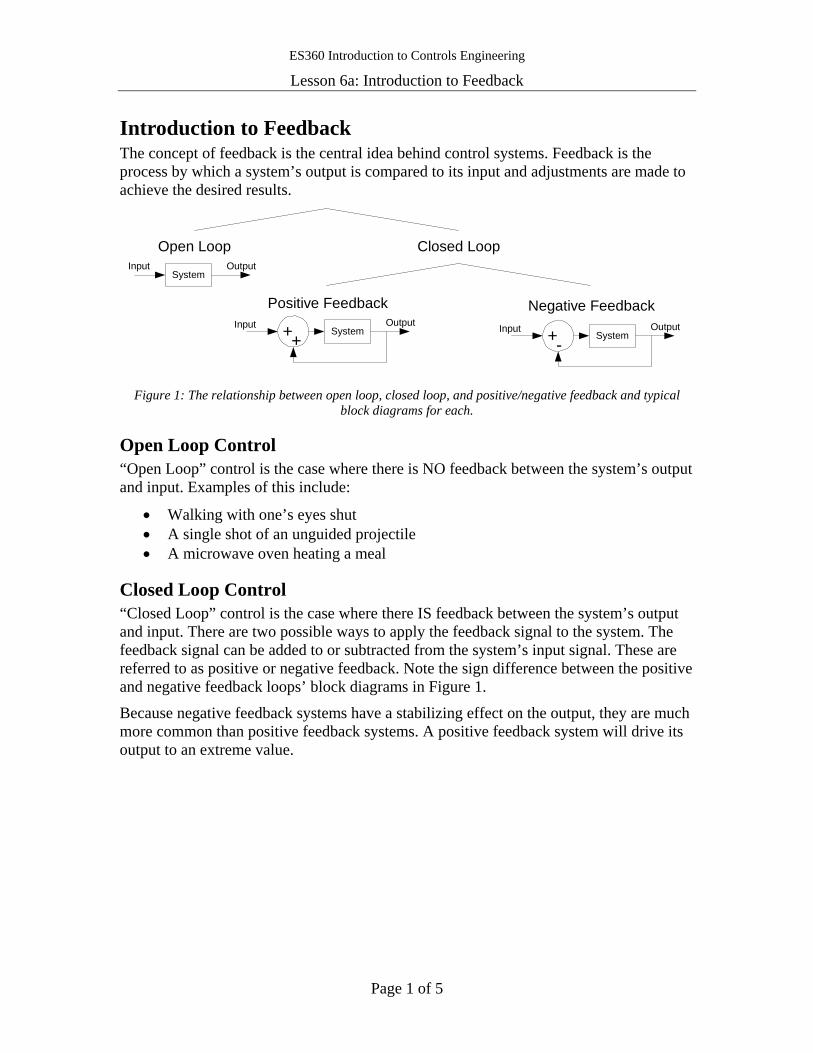
ES360 Introduction to Controls Engineering
Lesson 6a: Introduction to Feedback
Page 1 of 5
Introduction to Feedback The concept of feedback is the central idea behind control systems. Feedback is the process by which a system’s output is compared to its input and adjustments are made to achieve the desired results.
System+-Input OutputSystem++
Input Output
Open Loop Closed Loop
Negative FeedbackPositive Feedback
SystemInput Output
Figure 1: The relationship between open loop, closed loop, and positive/negative feedback and typical
block diagrams for each.
Open Loop Control “Open Loop” control is the case where there is NO feedback between the system’s output and input. Examples of this include:
• Walking with one’s eyes shut • A single shot of an unguided projectile • A microwave oven heating a meal
Closed Loop Control “Closed Loop” control is the case where there IS feedback between the system’s output and input. There are two possible ways to apply the feedback signal to the system. The feedback signal can be added to or subtracted from the system’s input signal. These are referred to as positive or negative feedback. Note the sign difference between the positive and negative feedback loops’ block diagrams in Figure 1.
Because negative feedback systems have a stabilizing effect on the output, they are much more common than positive feedback systems. A positive feedback system will drive its output to an extreme value.

ES360 Introduction to Controls Engineering
Lesson 6a: Introduction to Feedback
Page 2 of 5
An Automobile’s Cruise Control Example
The Negative Feedback Case
System+-R(s) C(s)E(s)
Figure 2: A simple negative feedback loop with the input R(s), error E(s), and output C(s) signals labeled.
The cruise control in a car is an excellent example of a negative feedback system.
Write the equation for the error signal E(s) for the negative feedback loop in Figure 2. Lesson 1b may be of some help.
E(s)=
If the error signal is positive, the control system opens the throttle more because the desired speed, R(s), is greater than actual speed, C(s). If the error signal is negative, the control system closes the throttle because desired speed, R(s), is less than actual speed, C(s). When the actual speed of the car is equal to the desired speed of the car, the error signal is zero and the control system does not change the throttle position.
If R(s), the desired speed, is set to 55mph and the actual speed of the car, C(s), is 45 mph, what is the value for E(s)? How does the cruise control change the throttle position?
E(s)=at 45mph
Throttle Position(circle one) Open More Close More Hold Position
As the car speeds up to 50 mph what happens to the magnitude of E(s)? How does the cruise control change the throttle position?
E(s)=at 50mph
Throttle Position(circle one) Open More Close More Hold Position
What is the value of E(s) at 55mph? How does the cruise control change the throttle position?
E(s)=at 55mph
Throttle Position(circle one) Open More Close More Hold Position
The car starts going down a hill and speeds up to 60 mph. What is the current value of E(s)? How does the cruise control change the throttle position?
E(s)=at 60mph
Throttle Position(circle one) Open More Close More Hold Position
Summary: This exercise has demonstrated how a negative feedback system regulates and stabilizes a system.
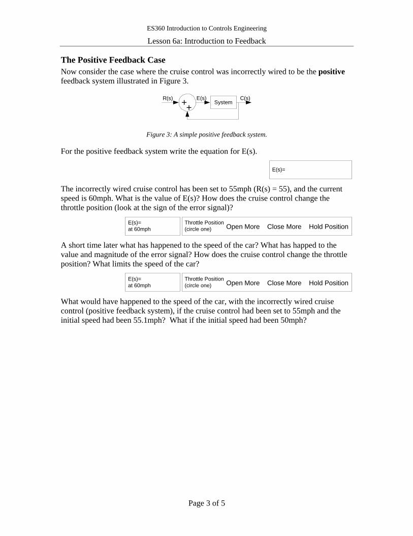
ES360 Introduction to Controls Engineering
Lesson 6a: Introduction to Feedback
Page 3 of 5
The Positive Feedback Case Now consider the case where the cruise control was incorrectly wired to be the positive feedback system illustrated in Figure 3.
System++R(s) C(s)E(s)
Figure 3: A simple positive feedback system.
For the positive feedback system write the equation for E(s).
E(s)=
The incorrectly wired cruise control has been set to 55mph (R(s) = 55), and the current speed is 60mph. What is the value of E(s)? How does the cruise control change the throttle position (look at the sign of the error signal)?
E(s)=at 60mph
Throttle Position(circle one) Open More Close More Hold Position
A short time later what has happened to the speed of the car? What has happed to the value and magnitude of the error signal? How does the cruise control change the throttle position? What limits the speed of the car?
E(s)=at 60mph
Throttle Position(circle one) Open More Close More Hold Position
What would have happened to the speed of the car, with the incorrectly wired cruise control (positive feedback system), if the cruise control had been set to 55mph and the initial speed had been 55.1mph? What if the initial speed had been 50mph?
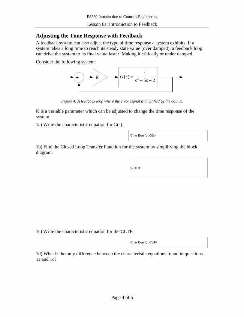
ES360 Introduction to Controls Engineering
Lesson 6a: Introduction to Feedback
Page 4 of 5
Adjusting the Time Response with Feedback A feedback system can also adjust the type of time response a system exhibits. If a system takes a long time to reach its steady state value (over damped), a feedback loop can drive the system to its final value faster. Making it critically or under damped.
Consider the following system:
+-
Figure 4: A feedback loop where the error signal is amplified by the gain K.
K is a variable parameter which can be adjusted to change the time response of the system.
1a) Write the characteristic equation for G(s).
Char Eqn for G(s)
1b) Find the Closed Loop Transfer Function for the system by simplifying the block diagram.
CLTF=
1c) Write the characteristic equation for the CLTF.
Char Eqn for CLTF
1d) What is the only difference between the characteristic equations found in questions 1a and 1c?
K 251)( 2 ++
=ss
sG
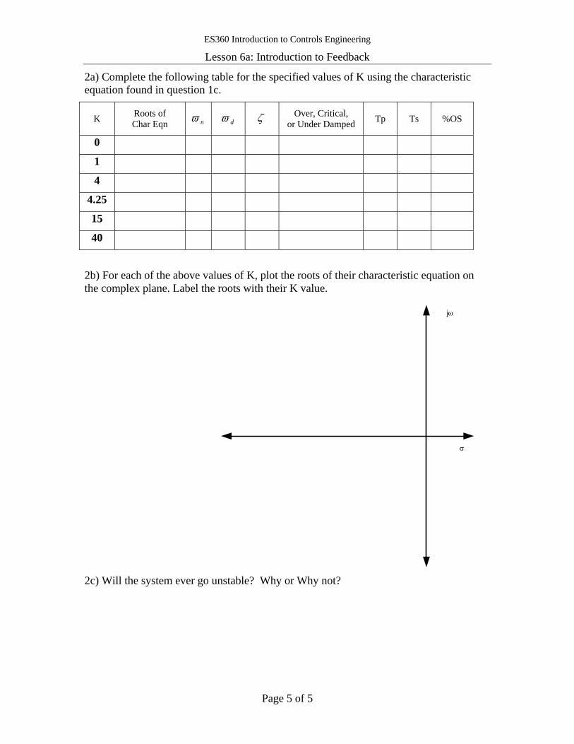
ES360 Introduction to Controls Engineering
Lesson 6a: Introduction to Feedback
Page 5 of 5
2a) Complete the following table for the specified values of K using the characteristic equation found in question 1c.
K Roots of Char Eqn nϖ dϖ ζ Over, Critical,
or Under Damped Tp Ts %OS
0
1
4
4.25
15
40
2b) For each of the above values of K, plot the roots of their characteristic equation on the complex plane. Label the roots with their K value.
σ
jω
2c) Will the system ever go unstable? Why or Why not?

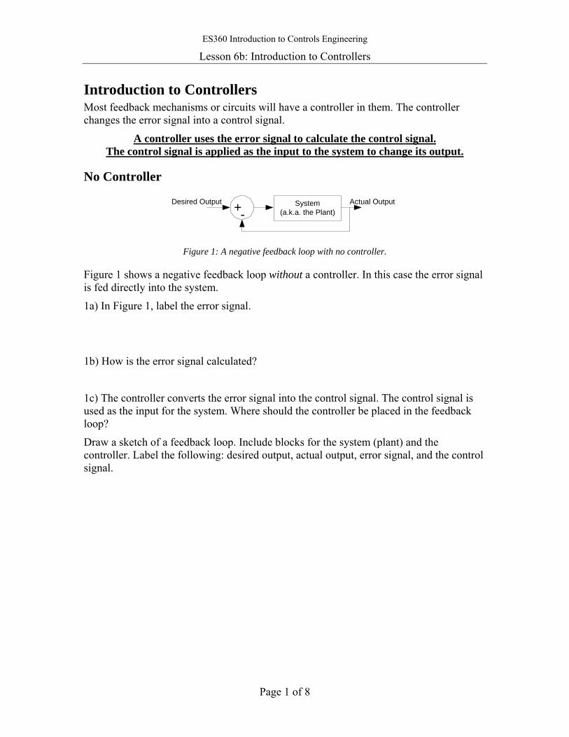
ES360 Introduction to Controls Engineering
Lesson 6b: Introduction to Controllers
Page 1 of 8
Introduction to Controllers Most feedback mechanisms or circuits will have a controller in them. The controller changes the error signal into a control signal.
A controller uses the error signal to calculate the control signal. The control signal is applied as the input to the system to change its output.
No Controller
System(a.k.a. the Plant)+-
Desired Output Actual Output
Figure 1: A negative feedback loop with no controller.
Figure 1 shows a negative feedback loop without a controller. In this case the error signal is fed directly into the system.
1a) In Figure 1, label the error signal.
1b) How is the error signal calculated?
1c) The controller converts the error signal into the control signal. The control signal is used as the input for the system. Where should the controller be placed in the feedback loop?
Draw a sketch of a feedback loop. Include blocks for the system (plant) and the controller. Label the following: desired output, actual output, error signal, and the control signal.
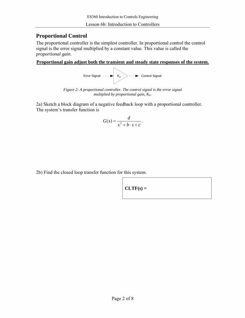
ES360 Introduction to Controls Engineering
Lesson 6b: Introduction to Controllers
Page 2 of 8
Proportional Control The proportional controller is the simplest controller. In proportional control the control signal is the error signal multiplied by a constant value. This value is called the proportional gain.
Proportional gain adjust both the transient and steady state responses of the system.
Control SignalError Signal KP
Figure 2: A proportional controller. The control signal is the error signal
multiplied by proportional gain, KP.
2a) Sketch a block diagram of a negative feedback loop with a proportional controller. The system’s transfer function is
csbsdsG
+⋅+= 2)( .
2b) Find the closed loop transfer function for this system.
CLTF(s) =
ES360 Introduction to Controls Engineering
Lesson 6b: Introduction to Controllers
Page 3 of 8
2c) In the closed loop transfer function, solve for the following in terms of KP, b, c, and d.
ωn = ζωn = ζ =
ωd = DC gain =
2d) Indicate how the following time response parameters change as the proportional gain, KP, increases.
Ts Tp %OS DC gain
2e) Does the proportional gain, KP, affect the steady state response of the system? Why or why not?
2f) Does the proportional gain affect the transient response (peak time, percent overshoot, etc.) of the system? Why or why not?
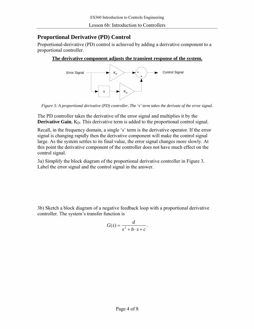
ES360 Introduction to Controls Engineering
Lesson 6b: Introduction to Controllers
Page 4 of 8
Proportional Derivative (PD) Control Proportional-derivative (PD) control is achieved by adding a derivative component to a proportional controller.
The derivative component adjusts the transient response of the system.
Control SignalError Signal KP+
+
KDs
Figure 3: A proportional derivative (PD) controller. The ‘s’ term takes the derivate of the error signal.
The PD controller takes the derivative of the error signal and multiplies it by the Derivative Gain, KD. This derivative term is added to the proportional control signal.
Recall, in the frequency domain, a single ‘s’ term is the derivative operator. If the error signal is changing rapidly then the derivative component will make the control signal large. As the system settles to its final value, the error signal changes more slowly. At this point the derivative component of the controller does not have much effect on the control signal.
3a) Simplify the block diagram of the proportional derivative controller in Figure 3. Label the error signal and the control signal in the answer.
3b) Sketch a block diagram of a negative feedback loop with a proportional derivative controller. The system’s transfer function is
csbsdsG
+⋅+= 2)( .
ES360 Introduction to Controls Engineering
Lesson 6b: Introduction to Controllers
Page 5 of 8
3c) Find the closed loop transfer function for this system.
CLTF(s) =
3d) Solve for the following in terms of KD, KP, b, c, and d.
ωn = ζωn = ζ =
ωd = DC gain =
3e) Indicate how the following time response parameters change as the derivative gain, KD, increases.
Ts Tp %OS DC gain
3f) Does the derivative gain, KD, affect the steady state response of the system? Why or why not?
3g) Does the derivative gain affect the transient response (peak time, percent overshoot, etc.) of the system? Why or why not?
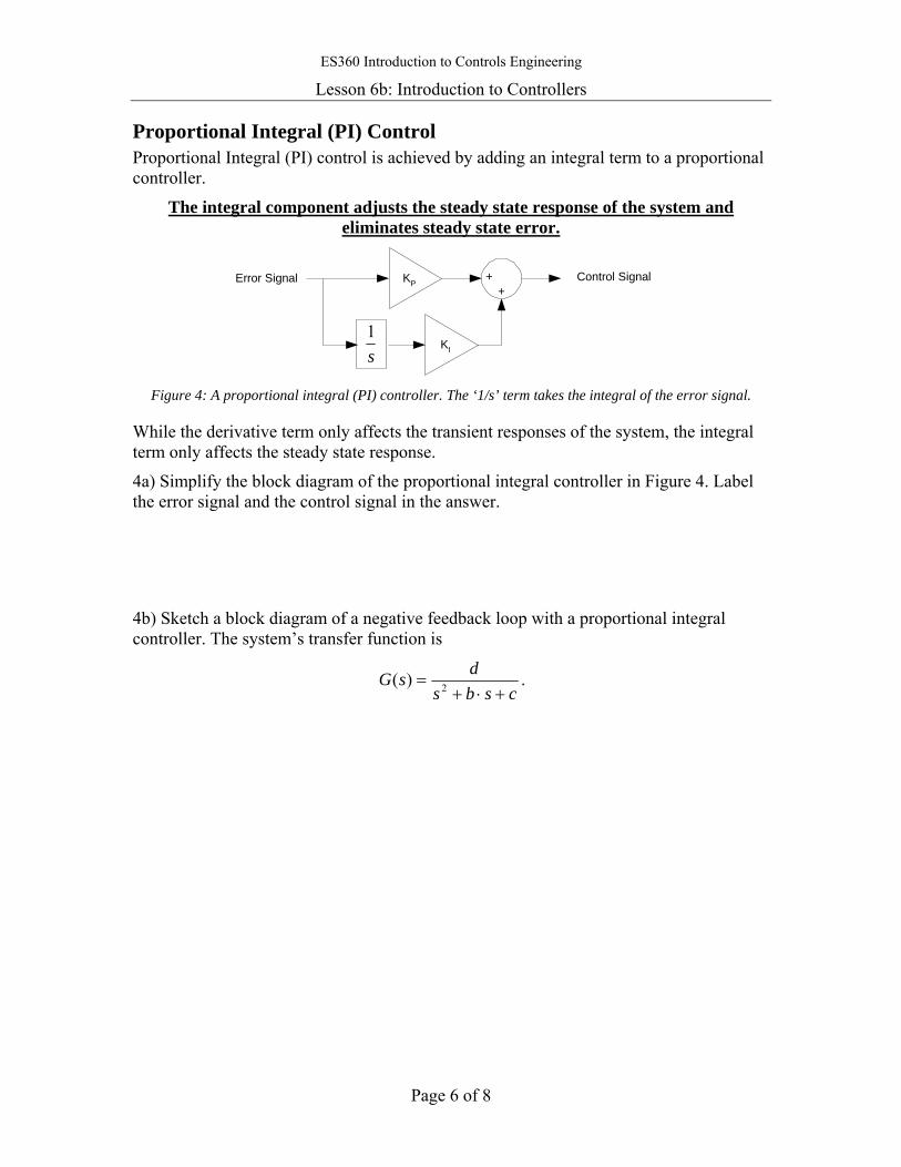
ES360 Introduction to Controls Engineering
Lesson 6b: Introduction to Controllers
Page 6 of 8
Proportional Integral (PI) Control Proportional Integral (PI) control is achieved by adding an integral term to a proportional controller.
The integral component adjusts the steady state response of the system and eliminates steady state error.
Control SignalError Signal KP+
+
KIs1
Figure 4: A proportional integral (PI) controller. The ‘1/s’ term takes the integral of the error signal.
While the derivative term only affects the transient responses of the system, the integral term only affects the steady state response.
4a) Simplify the block diagram of the proportional integral controller in Figure 4. Label the error signal and the control signal in the answer.
4b) Sketch a block diagram of a negative feedback loop with a proportional integral controller. The system’s transfer function is
csbsdsG
+⋅+= 2)( .
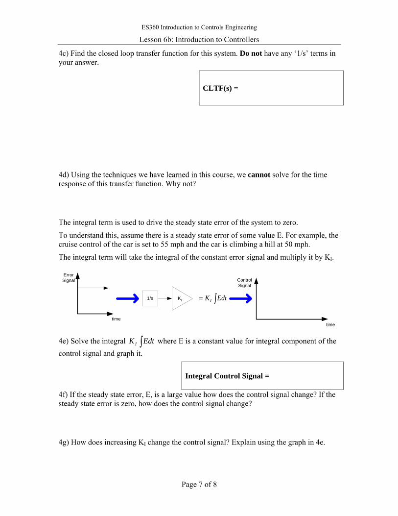
ES360 Introduction to Controls Engineering
Lesson 6b: Introduction to Controllers
Page 7 of 8
4c) Find the closed loop transfer function for this system. Do not have any ‘1/s’ terms in your answer.
CLTF(s) =
4d) Using the techniques we have learned in this course, we cannot solve for the time response of this transfer function. Why not?
The integral term is used to drive the steady state error of the system to zero.
To understand this, assume there is a steady state error of some value E. For example, the cruise control of the car is set to 55 mph and the car is climbing a hill at 50 mph.
The integral term will take the integral of the constant error signal and multiply it by KI.
KI1/s ∫= EdtKI
ControlSignal
time
ErrorSignal
time
4e) Solve the integral ∫ EdtK I where E is a constant value for integral component of the control signal and graph it.
Integral Control Signal =
4f) If the steady state error, E, is a large value how does the control signal change? If the steady state error is zero, how does the control signal change?
4g) How does increasing KI change the control signal? Explain using the graph in 4e.
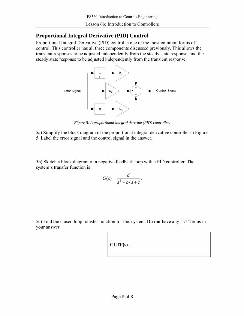
ES360 Introduction to Controls Engineering
Lesson 6b: Introduction to Controllers
Page 8 of 8
Proportional Integral Derivative (PID) Control Proportional Integral Derivative (PID) control is one of the most common forms of control. This controller has all three components discussed previously. This allows the transient responses to be adjusted independently from the steady state response, and the steady state response to be adjusted independently from the transient response.
Control SignalError Signal KP+
+
KDs
KI
+
s1
Figure 5: A proportional integral derivate (PID) controller.
5a) Simplify the block diagram of the proportional integral derivative controller in Figure 5. Label the error signal and the control signal in the answer.
5b) Sketch a block diagram of a negative feedback loop with a PID controller. The system’s transfer function is
csbsdsG
+⋅+= 2)( .
5c) Find the closed loop transfer function for this system. Do not have any ‘1/s’ terms in your answer
CLTF(s) =
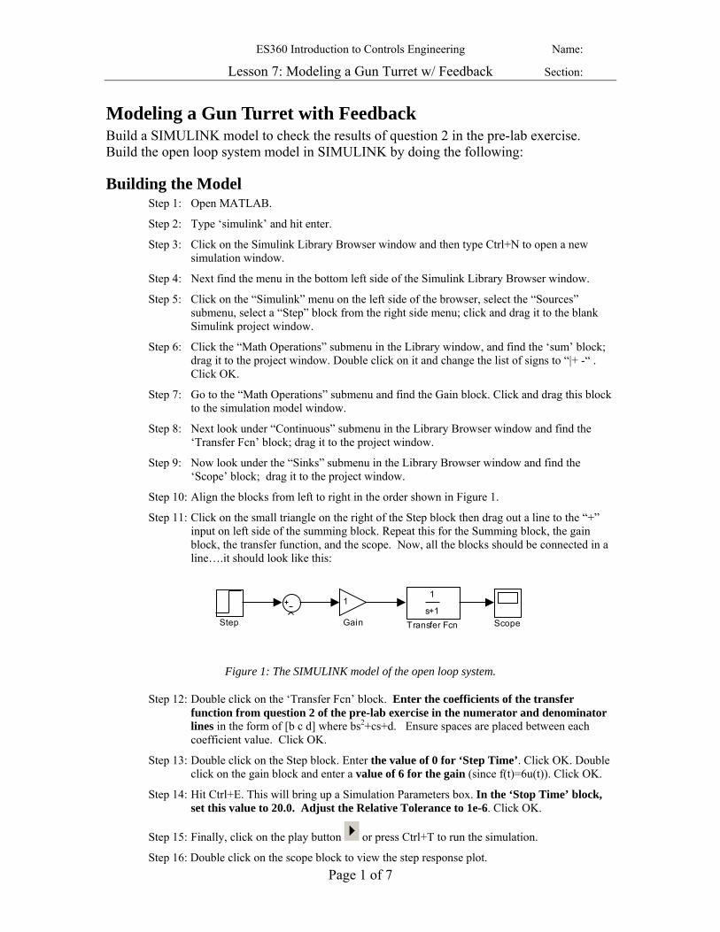
ES360 Introduction to Controls Engineering Name:
Lesson 7: Modeling a Gun Turret w/ Feedback Section:
Page 1 of 7
Modeling a Gun Turret with Feedback Build a SIMULINK model to check the results of question 2 in the pre-lab exercise. Build the open loop system model in SIMULINK by doing the following:
Building the Model Step 1: Open MATLAB.
Step 2: Type ‘simulink’ and hit enter.
Step 3: Click on the Simulink Library Browser window and then type Ctrl+N to open a new simulation window.
Step 4: Next find the menu in the bottom left side of the Simulink Library Browser window.
Step 5: Click on the “Simulink” menu on the left side of the browser, select the “Sources” submenu, select a “Step” block from the right side menu; click and drag it to the blank Simulink project window.
Step 6: Click the “Math Operations” submenu in the Library window, and find the ‘sum’ block; drag it to the project window. Double click on it and change the list of signs to “|+ -“ . Click OK.
Step 7: Go to the “Math Operations” submenu and find the Gain block. Click and drag this block to the simulation model window.
Step 8: Next look under “Continuous” submenu in the Library Browser window and find the ‘Transfer Fcn’ block; drag it to the project window.
Step 9: Now look under the “Sinks” submenu in the Library Browser window and find the ‘Scope’ block; drag it to the project window.
Step 10: Align the blocks from left to right in the order shown in Figure 1.
Step 11: Click on the small triangle on the right of the Step block then drag out a line to the “+” input on left side of the summing block. Repeat this for the Summing block, the gain block, the transfer function, and the scope. Now, all the blocks should be connected in a line….it should look like this:
1
s+1Transfer FcnStep Scope
1
Gain
Figure 1: The SIMULINK model of the open loop system.
Step 12: Double click on the ‘Transfer Fcn’ block. Enter the coefficients of the transfer function from question 2 of the pre-lab exercise in the numerator and denominator lines in the form of [b c d] where bs2+cs+d. Ensure spaces are placed between each coefficient value. Click OK.
Step 13: Double click on the Step block. Enter the value of 0 for ‘Step Time’. Click OK. Double click on the gain block and enter a value of 6 for the gain (since f(t)=6u(t)). Click OK.
Step 14: Hit Ctrl+E. This will bring up a Simulation Parameters box. In the ‘Stop Time’ block, set this value to 20.0. Adjust the Relative Tolerance to 1e-6. Click OK.
Step 15: Finally, click on the play button or press Ctrl+T to run the simulation.
Step 16: Double click on the scope block to view the step response plot.
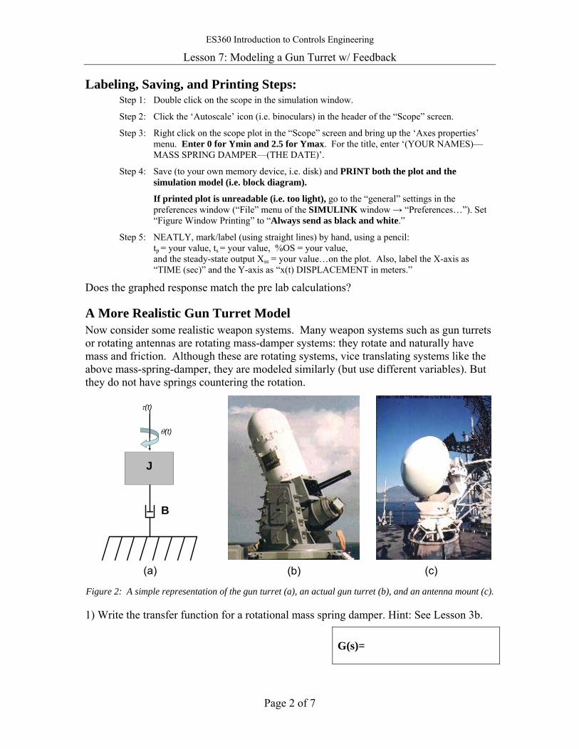
ES360 Introduction to Controls Engineering
Lesson 7: Modeling a Gun Turret w/ Feedback
Page 2 of 7
Labeling, Saving, and Printing Steps: Step 1: Double click on the scope in the simulation window.
Step 2: Click the ‘Autoscale’ icon (i.e. binoculars) in the header of the “Scope” screen.
Step 3: Right click on the scope plot in the “Scope” screen and bring up the ‘Axes properties’ menu. Enter 0 for Ymin and 2.5 for Ymax. For the title, enter ‘(YOUR NAMES)—MASS SPRING DAMPER—(THE DATE)’.
Step 4: Save (to your own memory device, i.e. disk) and PRINT both the plot and the simulation model (i.e. block diagram).
If printed plot is unreadable (i.e. too light), go to the “general” settings in the preferences window (“File” menu of the SIMULINK window → “Preferences…”). Set “Figure Window Printing” to “Always send as black and white.”
Step 5: NEATLY, mark/label (using straight lines) by hand, using a pencil: tp = your value, ts = your value, %OS = your value, and the steady-state output Xss = your value…on the plot. Also, label the X-axis as “TIME (sec)” and the Y-axis as “x(t) DISPLACEMENT in meters.”
Does the graphed response match the pre lab calculations?
A More Realistic Gun Turret Model Now consider some realistic weapon systems. Many weapon systems such as gun turrets or rotating antennas are rotating mass-damper systems: they rotate and naturally have mass and friction. Although these are rotating systems, vice translating systems like the above mass-spring-damper, they are modeled similarly (but use different variables). But they do not have springs countering the rotation.
B
J
τ(t)
θ(t)
(a) (b) (c) Figure 2: A simple representation of the gun turret (a), an actual gun turret (b), and an antenna mount (c).
1) Write the transfer function for a rotational mass spring damper. Hint: See Lesson 3b.
G(s)=

ES360 Introduction to Controls Engineering
Lesson 7: Modeling a Gun Turret w/ Feedback
Page 3 of 7
For this simulation use the following parameters: J=2000N-1-m-1-s-2 B= 1000 N-s τ(t)= 2000u(t) N-m (a step input). The gun turret has no spring.
2) Write the turret’s transfer function, substituting in the simulation parameters.
G(s)=
3) If you attempt to calculate θss, the steady state position of the gun turret, in response to a step input of torque, you get an unusual solution. Calculate it here:
θss=
4) Use your intuition to explain why this happens. If you apply a constant torque to a rotational mass with drag, will it stop at some particular position? Will it stop at all? Why is this different than a mass-spring-damper system?
Using SIMULINK to Investigate the Model 5) Simulate the step response of this open-loop system using the model developed in question 2.
Step 1: Double click on the ‘Transfer Fcn’ block. Enter the coefficients of the transfer function from question 2 into the numerator and denominator in the form of [b c d] where bs2+cs+d. Ensure spaces are placed between each coefficient value. Click OK.
Step 2: Double click on the gain block and enter 2000 [since τ(t)=2000u(t)]. Click OK. Click and drag on the gain block to make it larger. This will allow you to see the gain value.
Step 3: Finally, click on the play button or press Ctrl+T to run the simulation.
Plot the result as follows: Step 1: Double click on the scope in the simulation window.
Step 2: Click the ‘Autoscale’ icon (i.e. binoculars) in the header of the “Scope” screen.
Step 3: Right click on the scope plot in the “Scope” screen and bring up the ‘Axes properties’ menu. For the title, enter ‘(YOUR NAMES)—Gun Turret Step Response Without Feedback—(THE DATE)’.
Step 4: Print both the plot and the simulation model (i.e. block diagram).
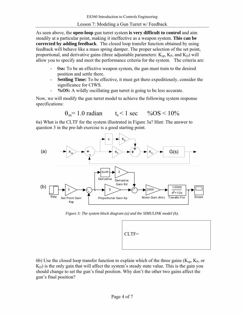
ES360 Introduction to Controls Engineering
Lesson 7: Modeling a Gun Turret w/ Feedback
Page 4 of 7
As seen above, the open-loop gun turret system is very difficult to control and aim steadily at a particular point, making it ineffective as a weapon system. This can be corrected by adding feedback. The closed loop transfer function obtained by using feedback will behave like a mass spring damper. The proper selection of the set point, proportional, and derivative gains (three adjustable parameters: Ksp, KP, and KD) will allow you to specify and meet the performance criteria for the system. The criteria are:
- θss: To be an effective weapon system, the gun must train to the desired position and settle there.
- Settling Time: To be effective, it must get there expeditiously, consider the significance for CIWS.
- %OS: A wildly oscillating gun turret is going to be less accurate.
Now, we will modify the gun turret model to achieve the following system response specifications:
θss= 1.0 radian ts < 1 sec %OS < 10% 6a) What is the CLTF for the system illustrated in Figure 3a? Hint: The answer to question 3 in the pre-lab exercise is a good starting point.
(a)
(b)
G(s)++ Km+- KP
KD
Ksp
s
1/2000
s +1/2s2
Transfer FcnStep
5
Set Point GainKsp
Scope
5
Proportional Gain Kp
2000
Motor Gain (Km)
5
DerivativeGain Kd
du/dt
Derivative
Figure 3: The system block diagram (a) and the SIMULINK model (b).
CLTF=
6b) Use the closed loop transfer function to explain which of the three gains (Ksp, KP, or KD) is the only gain that will affect the system’s steady state value. This is the gain you should change to set the gun’s final position. Why don’t the other two gains affect the gun’s final position?
ES360 Introduction to Controls Engineering
Lesson 7: Modeling a Gun Turret w/ Feedback
Page 5 of 7
7) Now we are going to use SIMULINK to iteratively find the controller gain values (Ksp, KP, and KD) which will meet the above requirements. Pick a value for each feedback constant, and adjust them until the above performance requirements are met. Write the final values in the spaces below. Do NOT get your values from other lab groups.
Using SIMULINK, model the system. Your block diagram should include the original blocks the pre-lab model, and will look like the diagram in Figure 3b after the following steps 1 to 12 below. Your values for the forward path gain, feedback gains and the transfer function should have been inserted. To see the values in the boxes, expand the boxes horizontally by clicking and dragging a box corner.
Step 1: Label the gain block to the left of the transfer function block ‘Motor Gain (Km)’.
Step 2: Click, then delete, the line from the sum block to the motor gain block .
Step 3: Click on the Library Browser window.
Step 4: Go to the “Math Operations” submenu and find the Gain block. Click and drag this block to the simulation model window three (3) times. Alternatively, you can use the copy and paste commands to duplicate the gain block.
Step 5: Go to the “Math Operations” submenu and find the Sum block. Click and drag this block to the simulation model window. Double click on the sum block and set the list of signs to ‘++|’. Move the this sum block to the left of the motor gain block.
Step 6: Click on the “Continuous” submenu in the Library Browser window and click on the Derivative. Drag one of these blocks to the simulation window.
Step 7: Place two gain blocks between the sum blocks, one below the other.
Step 8: Place the derivative block to the left of the upper Gain block.
Step 9: Place the last Gain block between the Step block and first Summing junction.
Step 10: Connect the blocks as illustrated in Figure 3b.
Step 11: Double click on the Gain blocks and enter your estimated values.
Left click on the three gain title blocks and properly rename them as “Set Point Gain Ksp”, “Proportional Gain Kp”, and “Derivative Gain Kd” as appropriate.
Step 12: Adjust your ‘Simulation Parameters’ using Ctrl+E:
Stop Time = 3 seconds, Relative Tolerance = 1e-6.
ES360 Introduction to Controls Engineering
Lesson 7: Modeling a Gun Turret w/ Feedback
Page 6 of 7
Run the simulation and verify your system meets the specs. It should, very closely. If not, recheck your math, correct errors, and try again. Once it meets the specs, print the results:
Step 1: Double click on the scope in the simulation window.
Step 2: Click the ‘Autoscale’ icon (i.e. binoculars) ) in the header of the “Scope” screen.
Step 3: Right click on the scope plot in the “Scope” screen and bring up the ‘Axes properties’ menu. For the title, enter ‘(YOUR NAME)—System Response With Feedback—(THE DATE)’. Click OK>
Step 4: PRINT both the plot and the simulation model (i.e. block diagram). Your name should be typed on the block diagram print out.
Step 5: NEATLY, mark/label (using straight lines) by hand using a pencil:
tp = your value, ts = your value, %PO = your value, and the steady-state output θss = your value…on the plot. Also, label the X-axis as “TIME (sec)” and the Y-axis as “θ(t) in radians.”
Ksp=
Set Point Gain
KP=
Proportional Gain
KD=
Derivative Gain

ES360 Introduction to Controls Engineering
Lesson 7: Modeling a Gun Turret w/ Feedback
Page 7 of 7
Feedback Malfunctions Now investigate (printed plots not required) the effects of some malfunctions of the control system. You should sketch a plot of the response as part of your answer. First use Ctrl-E to set stop time to 10 seconds, then simulate.
8) What happens if derivative control lost? Set KD to zero, and run the simulation.
9) What happens if proportional control is lost? Restore your original value of KD, set KP to zero, and run the simulation.
10) What happens if proportional control is reduced by 90%? Set the proportional gain to 10% of your original value and run the simulation.
11) What happens if the set point gain is reduced by 50%? Restore KP to your original value, set Ksp to half your original value, and run the simulation.
12) What happens if the feedback signal is lost? Restore Ksp to your original value, delete the feedback line, and run the simulation.
For this assignment to be complete you must include the printouts of the 3 block diagrams, and three output plots.

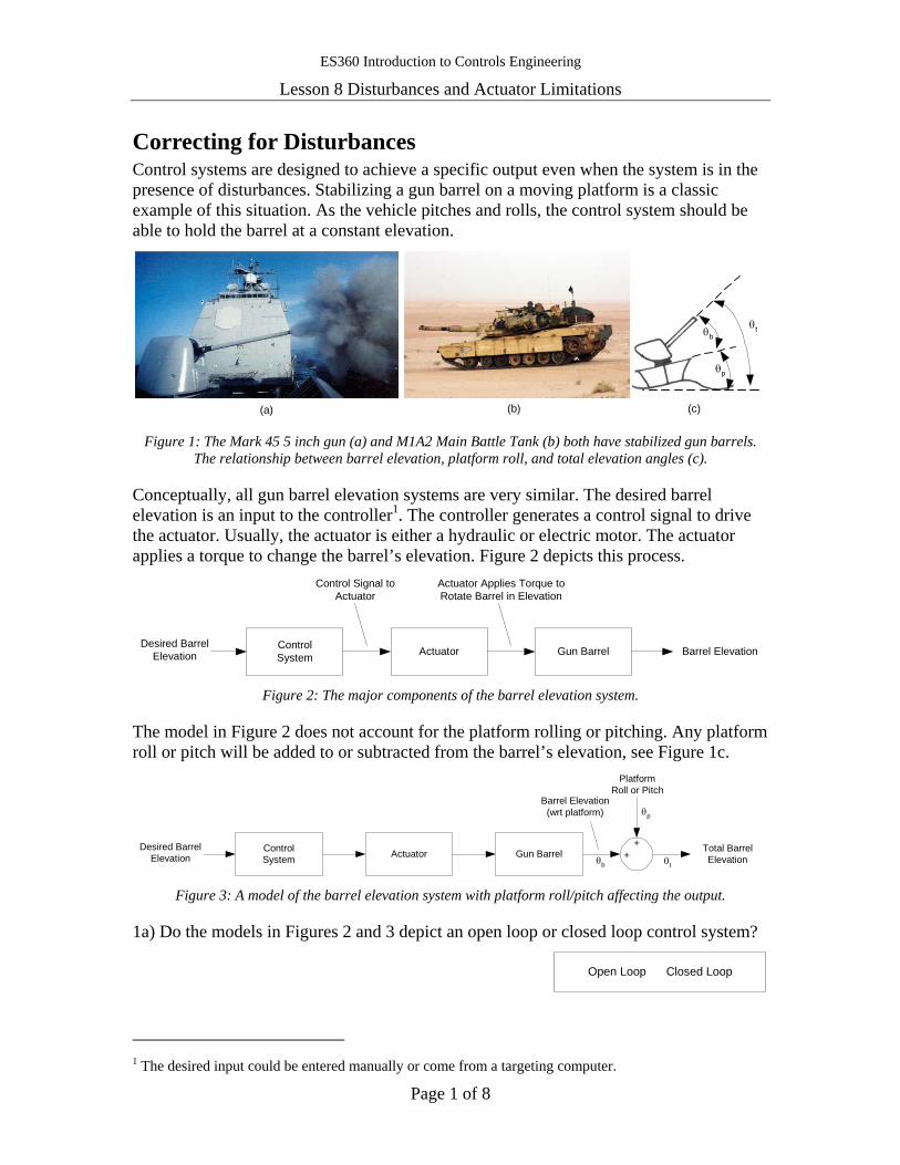
ES360 Introduction to Controls Engineering
Lesson 8 Disturbances and Actuator Limitations
Page 1 of 8
Correcting for Disturbances Control systems are designed to achieve a specific output even when the system is in the presence of disturbances. Stabilizing a gun barrel on a moving platform is a classic example of this situation. As the vehicle pitches and rolls, the control system should be able to hold the barrel at a constant elevation.
(a) (b)
θb
θp
θt
(c) Figure 1: The Mark 45 5 inch gun (a) and M1A2 Main Battle Tank (b) both have stabilized gun barrels.
The relationship between barrel elevation, platform roll, and total elevation angles (c).
Conceptually, all gun barrel elevation systems are very similar. The desired barrel elevation is an input to the controller1. The controller generates a control signal to drive the actuator. Usually, the actuator is either a hydraulic or electric motor. The actuator applies a torque to change the barrel’s elevation. Figure 2 depicts this process.
ActuatorControlSystem Gun Barrel
Desired BarrelElevation
Control Signal toActuator
Actuator Applies Torque toRotate Barrel in Elevation
Barrel Elevation
Figure 2: The major components of the barrel elevation system.
The model in Figure 2 does not account for the platform rolling or pitching. Any platform roll or pitch will be added to or subtracted from the barrel’s elevation, see Figure 1c.
ActuatorControlSystem Gun Barrel
Desired BarrelElevation
Barrel Elevation(wrt platform)
PlatformRoll or Pitch
Total BarrelElevation
++θb θt
θp
Figure 3: A model of the barrel elevation system with platform roll/pitch affecting the output.
1a) Do the models in Figures 2 and 3 depict an open loop or closed loop control system?
Open Loop Closed Loop
1 The desired input could be entered manually or come from a targeting computer.
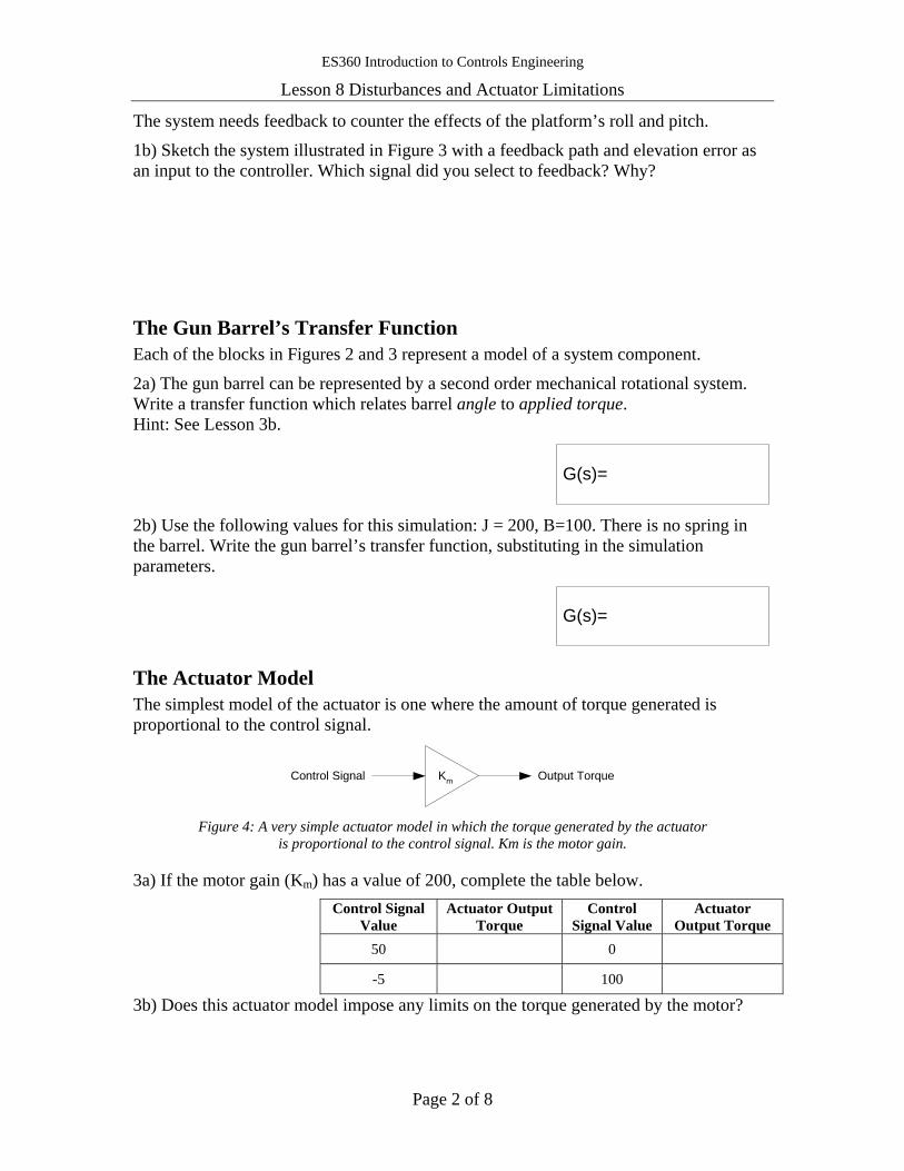
ES360 Introduction to Controls Engineering
Lesson 8 Disturbances and Actuator Limitations
Page 2 of 8
The system needs feedback to counter the effects of the platform’s roll and pitch.
1b) Sketch the system illustrated in Figure 3 with a feedback path and elevation error as an input to the controller. Which signal did you select to feedback? Why?
The Gun Barrel’s Transfer Function Each of the blocks in Figures 2 and 3 represent a model of a system component.
2a) The gun barrel can be represented by a second order mechanical rotational system. Write a transfer function which relates barrel angle to applied torque. Hint: See Lesson 3b.
G(s)=
2b) Use the following values for this simulation: J = 200, B=100. There is no spring in the barrel. Write the gun barrel’s transfer function, substituting in the simulation parameters.
G(s)=
The Actuator Model The simplest model of the actuator is one where the amount of torque generated is proportional to the control signal.
Km Output TorqueControl Signal
Figure 4: A very simple actuator model in which the torque generated by the actuator
is proportional to the control signal. Km is the motor gain.
3a) If the motor gain (Km) has a value of 200, complete the table below. Control Signal
Value Actuator Output
Torque Control
Signal Value Actuator
Output Torque 50 0
-5 100
3b) Does this actuator model impose any limits on the torque generated by the motor?
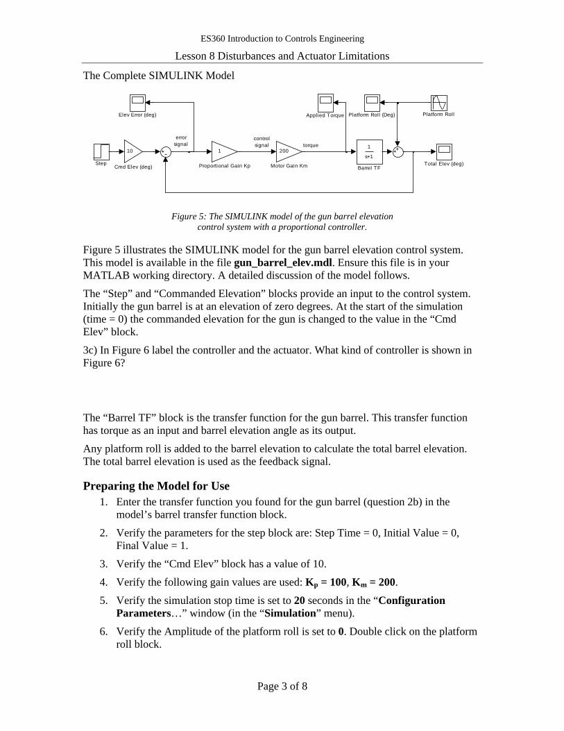
ES360 Introduction to Controls Engineering
Lesson 8 Disturbances and Actuator Limitations
Page 3 of 8
The Complete SIMULINK Model
controlsignal torque
errorsignal
Total Elev (deg)Step
1
Proportional Gain Kp
Platform Roll (Deg) Platform Roll
200
Motor Gain Km
Elev Error (deg)
10
Cmd Elev (deg)
1
s+1
Barrel TF
Applied Torque
Figure 5: The SIMULINK model of the gun barrel elevation
control system with a proportional controller.
Figure 5 illustrates the SIMULINK model for the gun barrel elevation control system. This model is available in the file gun_barrel_elev.mdl. Ensure this file is in your MATLAB working directory. A detailed discussion of the model follows.
The “Step” and “Commanded Elevation” blocks provide an input to the control system. Initially the gun barrel is at an elevation of zero degrees. At the start of the simulation (time = 0) the commanded elevation for the gun is changed to the value in the “Cmd Elev” block.
3c) In Figure 6 label the controller and the actuator. What kind of controller is shown in Figure 6?
The “Barrel TF” block is the transfer function for the gun barrel. This transfer function has torque as an input and barrel elevation angle as its output.
Any platform roll is added to the barrel elevation to calculate the total barrel elevation. The total barrel elevation is used as the feedback signal.
Preparing the Model for Use 1. Enter the transfer function you found for the gun barrel (question 2b) in the
model’s barrel transfer function block.
2. Verify the parameters for the step block are: Step Time = 0, Initial Value = 0, Final Value = 1.
3. Verify the “Cmd Elev” block has a value of 10.
4. Verify the following gain values are used: Kp = 100, Km = 200.
5. Verify the simulation stop time is set to 20 seconds in the “Configuration Parameters…” window (in the “Simulation” menu).
6. Verify the Amplitude of the platform roll is set to 0. Double click on the platform roll block.

ES360 Introduction to Controls Engineering
Lesson 8 Disturbances and Actuator Limitations
Page 4 of 8
Testing the Model with No Platform Roll 4a) Make a sketch of the complete model. You do not need to include the “scope”, “step”, or “Cmd Elev” blocks in your sketch.
4b) Assuming there is NO platform roll, find the closed loop transfer function for the system sketched in question 4a. No platform roll means the platform roll block and its summing junction can be ignored when finding the CLTF. Additionally, do not include the step input block or “commanded elevation” block.
CLTF(s)=
4c) Solve for the following, using the closed loop transfer function found in question 4b.
Response Type Ts %OS
4d) Calculate the steady state gun barrel elevation for a command elevation of 10 degrees applied as a step input. Hint: Use the final value theorem.
θss
ES360 Introduction to Controls Engineering
Lesson 8 Disturbances and Actuator Limitations
Page 5 of 8
4e) Verify your answers to questions 4c and 4d with the SIMULINK model. Run the model by clicking the button in the model window. Display the plots of Elevation Error, Applied Torque, and Barrel Elevation by double clicking on the scope blocks in the model. You may need to click the button in the plot windows to set the axis limits properly. Estimate the following values from the plots.
Response Type Ts %OS
4f) Did the simulation match your calculations? Does this seem like good performance for a gun barrel with NO platform motion?
A Better Controller (proportional derivative) To improve the response of the gun barrel replace the proportional controller with a proportional derivative controller. Hint: See Lesson 6b.
5a) Make a sketch of the complete model with PD control. You do not need to include the the “scope”, “step”, or “Cmd Elev” blocks in your sketch.
5b) Assuming there is NO platform roll, find the closed loop transfer function for the system sketched in question 5a. No platform roll means the platform roll block and its summing junction can be ignored when finding the CLTF. Additionally, do not include the step input block or “commanded elevation” block. Leave KP and KD as variables.
CLTF(s)=
5c) Using the closed loop transfer function found in question 5b and KP = 100 and KD = 10, solve for the following:
Response Type Ts %OS
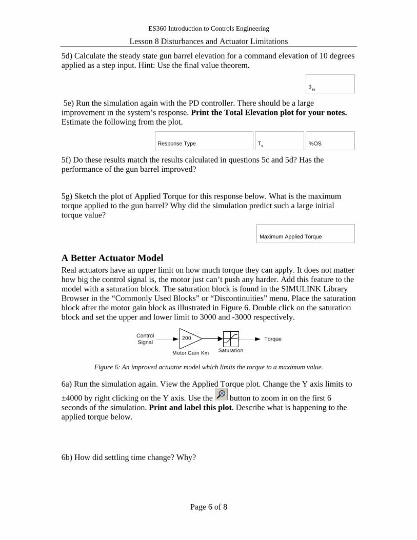
ES360 Introduction to Controls Engineering
Lesson 8 Disturbances and Actuator Limitations
Page 6 of 8
5d) Calculate the steady state gun barrel elevation for a command elevation of 10 degrees applied as a step input. Hint: Use the final value theorem.
θss 5e) Run the simulation again with the PD controller. There should be a large improvement in the system’s response. Print the Total Elevation plot for your notes. Estimate the following from the plot.
Response Type Ts %OS 5f) Do these results match the results calculated in questions 5c and 5d? Has the performance of the gun barrel improved?
5g) Sketch the plot of Applied Torque for this response below. What is the maximum torque applied to the gun barrel? Why did the simulation predict such a large initial torque value?
Maximum Applied Torque
A Better Actuator Model Real actuators have an upper limit on how much torque they can apply. It does not matter how big the control signal is, the motor just can’t push any harder. Add this feature to the model with a saturation block. The saturation block is found in the SIMULINK Library Browser in the “Commonly Used Blocks” or “Discontinuities” menu. Place the saturation block after the motor gain block as illustrated in Figure 6. Double click on the saturation block and set the upper and lower limit to 3000 and -3000 respectively.
ControlSignal
Saturation
200
Motor Gain Km
Torque
Figure 6: An improved actuator model which limits the torque to a maximum value.
6a) Run the simulation again. View the Applied Torque plot. Change the Y axis limits to
±4000 by right clicking on the Y axis. Use the button to zoom in on the first 6 seconds of the simulation. Print and label this plot. Describe what is happening to the applied torque below.
6b) How did settling time change? Why?
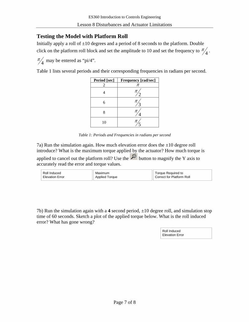
ES360 Introduction to Controls Engineering
Lesson 8 Disturbances and Actuator Limitations
Page 7 of 8
Testing the Model with Platform Roll Initially apply a roll of ±10 degrees and a period of 8 seconds to the platform. Double click on the platform roll block and set the amplitude to 10 and set the frequency to 4
π .
4π may be entered as “pi/4”.
Table 1 lists several periods and their corresponding frequencies in radians per second.
Table 1: Periods and Frequencies in radians per second
7a) Run the simulation again. How much elevation error does the ±10 degree roll introduce? What is the maximum torque applied by the actuator? How much torque is applied to cancel out the platform roll? Use the button to magnify the Y axis to accurately read the error and torque values.
Roll InducedElevation Error
MaximumApplied Torque
Torque Required toCorrect for Platform Roll
7b) Run the simulation again with a 4 second period, ±10 degree roll, and simulation stop time of 60 seconds. Sketch a plot of the applied torque below. What is the roll induced error? What has gone wrong?
Roll InducedElevation Error
Period [sec] Frequency [rad/sec] 2 π
4 2π
6 3π
8 4π
10 5π

ES360 Introduction to Controls Engineering
Lesson 8 Disturbances and Actuator Limitations
Page 8 of 8
7c) Set KP = 100 and KD = 10. Set the maximum torque of the motor to 9,000 Nm, by changing the upper and lower limits for the saturation block. Re-run the simulation. How does this improve the response, and why?
7d) Based on the results of this lab, what are two methods of improving a system’s ability to compensate for disturbances? Why?
ES360 Introduction to Controls Engineering
Lesson 9: PID Controllers
Page 1 of 13
Lesson 9: PID Controllers
The Generator Set Model The goal of this lesson is to control the frequency output of an AC generator set as the electrical load placed on the generator changes.1
Figure 1: A Caterpillar diesel generator set and a General Electric LM2500 gas turbine generator set.
1a) What determines the output frequency of an AC generator?
1b) What determines the required torque of an AC generator?
1c) As the loading of the generator increases, how does the required torque to rotate the generator change? What happens to the generator’s speed?
In this simplified model, the generator is rotated by an engine which is controlled by a controller.
Controller Engine Generator
Control SignalError Signal Torque Generator Speed (RPM)Desired Speed (RPM)
-+
Figure 2: The conceptual diagram of the model to control generator speed.
The engine is modeled as a 1st order system with the transfer function
1100)(+
=s
sGE .
1 The term “generator set” refers to the whole machine (i.e. controller, engine, and generator). The term “generator” refers to just the device which converts rotational motion to electricity.
ES360 Introduction to Controls Engineering
Lesson 9: PID Controllers
Page 2 of 13
The electrical generator is modeled as a 1st order rotational mechanical system with the transfer function
JB
JG s
sG+
=1
)(
where J is the rotational inertia of the generator and B is the friction coefficient for the generator. The generator’s transfer function has torque as its input and rotational speed as its output. The output frequency of the generator is determined by its rotational speed. The control system should maintain the required generator speed, and thereby output frequency, under a wide range of loading conditions.
As a larger electrical load is placed on the generator, more torque is required to keep the generator spinning at the same speed. This is analogous to adding more friction into the system. In a mechanical rotational system the relationship for friction is
ϖτ B=
where ω is rotational speed, B the frictional coefficient, and τ is torque. Adding more friction to the system increases the magnitude of B. In this model there are two sources of friction in the generator. The internal friction of the generator, GB , and the “friction” created by the electrical load on the generator, LB . Specifying both of the frictional terms in the generator’s transfer function yields
JBB
JG LGs
sG ++=
1
)( .
The block diagram for this transfer function is drawn with the frictional terms as separate blocks. This makes it easier for the simulation to vary the friction due to electrical loading, LB .
-+
BG
BL
+
+
S1
J1
Figure 3: The block diagram of the generator transfer function.
2) Simplify the block diagram in Figure 3 to show that it is equivalent to )(sGG listed above. Show the intermediate diagrams.
G(s)=
ES360 Introduction to Controls Engineering
Lesson 9: PID Controllers
Page 3 of 13
The Open Loop Model of the Generator Set Imagine there is no feedback and no controller in the generator set. The throttle on the engine is set to 1800 RPM and never changed.
3a) What will happen to generator speed as loading is increased? Why?
3b) Sketch an open loop block diagram with the appropriate transfer functions for the engine and generator. J = 1000 and BG = 100. Leave BL as a variable.
3c) Simplify the block diagram and write the resulting transfer function.
3d) Using the final value theorem, calculate the final values for the open loop system. The input is a step input of 1800 RPM. What happens to generator speed as loading is increased? Why?
BL Final Value
0
10
100
1,000
100,000
3e) Do the results in question 3d match your prediction in question 3a? How effective is open loop control in this application?
ES360 Introduction to Controls Engineering
Lesson 9: PID Controllers
Page 4 of 13
Proportional Control 4a) Sketch a proportional controller. Label the error signal and control signal. Hint: See Lesson 6b.
4b) How is the error signal for the controller generated?
4c) How is the control signal generated? Hint: See Lesson 6b.
4d) Sketch a block diagram of the complete generator set model with a proportional controller and the transfer functions for the engine and generator. Use the generator transfer function model from Figure 3. J = 1000 and BG = 100. Leave BL as a variable.
4e) Simplify the block diagram in question 4d to find the closed loop transfer function for the system. Hint: Use the solution found in question 2 of the pre-lab with KD set to zero.

ES360 Introduction to Controls Engineering
Lesson 9: PID Controllers
Page 5 of 13
4f) From your answer in 4e, calculate the proportional gain (KP) required to keep the generator speed at full load (BL=100,000) within 5% of its initial value. This means the DC gain of the closed loop transfer function found in 4c should be at least 0.95.
Kp=
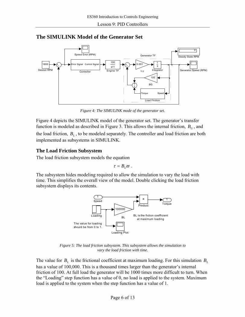
ES360 Introduction to Controls Engineering
Lesson 9: PID Controllers
Page 6 of 13
The SIMULINK Model of the Generator Set
Generator TF
0
Steady State RPMSpeed Error (RPM)
SpeedTorque
Load Friction
1s
Integrator Generator Speed (RPM)
100
s+1Engine TF
1800
Desired RPM
Error Signal Control Signal
Controller
100
BG
0.001
1/J
Figure 4: The SIMULINK mode of the generator set.
Figure 4 depicts the SIMULINK model of the generator set. The generator’s transfer function is modeled as described in Figure 3. This allows the internal friction, GB , and the load friction, LB , to be modeled separately. The controller and load friction are both implemented as subsystems in SIMULINK.
The Load Friction Subsystem The load friction subsystem models the equation
ϖτ LB= .
The subsystem hides modeling required to allow the simulation to vary the load with time. This simplifies the overall view of the model. Double clicking the load friction subsystem displays its contents.
The value for loadingshould be from 0 to 1.
BL is the fiction coefficientat maximum loading
1TorqueProduct
Loading Plot
Loading
100000
BL
1Speed
Figure 5: The load friction subsystem. This subsystem allows the simulation to
vary the load friction with time.
The value for LB is the frictional coefficient at maximum loading. For this simulation LB has a value of 100,000. This is a thousand times larger than the generator’s internal friction of 100. At full load the generator will be 1000 times more difficult to turn. When the “Loading” step function has a value of 0, no load is applied to the system. Maximum load is applied to the system when the step function has a value of 1.

ES360 Introduction to Controls Engineering
Lesson 9: PID Controllers
Page 7 of 13
Preparing the Model for Use 1. Download the model file generator.mdl to your work area and open it in
SIMULINK.
2. Set Simulation Stop Time to 20 seconds (Set in the Simulation Menu → Configuration Parameters…).
3. Set the following values: Desired RPM = 1800, BG=100, 1/J= 0.001
4. In the “Load Friction” subsystem:
a. BL=100,000
b. Loading Step Input: Initial Value = 0, Final Value = 1, Step Time = 10
Testing the Proportional Controller 4g) Verify the answer to question 4d with the SIMULINK model of the generator. After setting the model up for use, implement a proportional controller in the “Controller” subsystem. Use the gain value calculated in question 4f. Print the “Generator Speed” plot for your notes.
• Label it as “Generator No Load Step Response”.
• Annotate your Kp value on the plot.
• Annotate the point on the plot where full load is applied.
• What is the steady state generator speed at the end of the simulation? Is this within 5% of the desired RPM of 1800?
Final RPM= Kp=
4h) Initially the generator set is shutdown (0 RPM). At time zero the generator set gets started and the controller immediately tries to regulate generator speed to 1800 RPM. How good is the transient response between 0 and 10 seconds? What is the response type?
4i) After full loading is applied, at 10 seconds, the generator’s output is much smoother than it was for the first 10 seconds of the simulation. Why?
4j) Try to improve the transient response by lowering the gain KP in the controller. Does this improve the transient response? As KP is lowered, what happens to the steady state response (the final generator speed) at full load?
ES360 Introduction to Controls Engineering
Lesson 9: PID Controllers
Page 8 of 13
Proportional-Derivative (PD) Control 5a) Sketch a proportional derivative controller. Label the error signal and control signal.
5b) Write an expression for the control signal in terms of the error signal?
5c) Sketch a block diagram of the complete generator set model with a proportional-derivative controller and the transfer functions for the engine and generator. Use the generator transfer function model from Figure 3. J = 1000 and BG = 100. Leave BL as a variable.
5d) Simplify the block diagram in question 5c to find the closed loop transfer function for the system. Hint: Use the answer to question 2 of the pre-lab exercise.
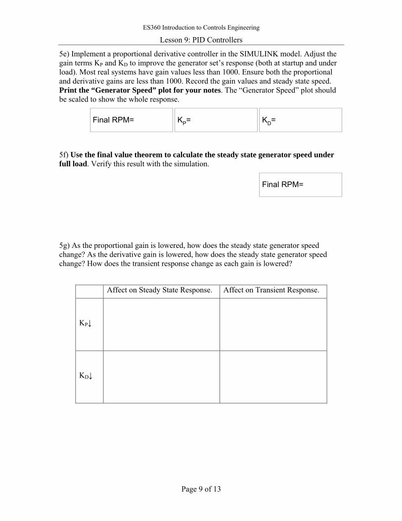
ES360 Introduction to Controls Engineering
Lesson 9: PID Controllers
Page 9 of 13
5e) Implement a proportional derivative controller in the SIMULINK model. Adjust the gain terms KP and KD to improve the generator set’s response (both at startup and under load). Most real systems have gain values less than 1000. Ensure both the proportional and derivative gains are less than 1000. Record the gain values and steady state speed. Print the “Generator Speed” plot for your notes. The “Generator Speed” plot should be scaled to show the whole response.
Final RPM= KP= KD=
5f) Use the final value theorem to calculate the steady state generator speed under full load. Verify this result with the simulation.
Final RPM=
5g) As the proportional gain is lowered, how does the steady state generator speed change? As the derivative gain is lowered, how does the steady state generator speed change? How does the transient response change as each gain is lowered?
Affect on Steady State Response. Affect on Transient Response.
KP↓
KD↓
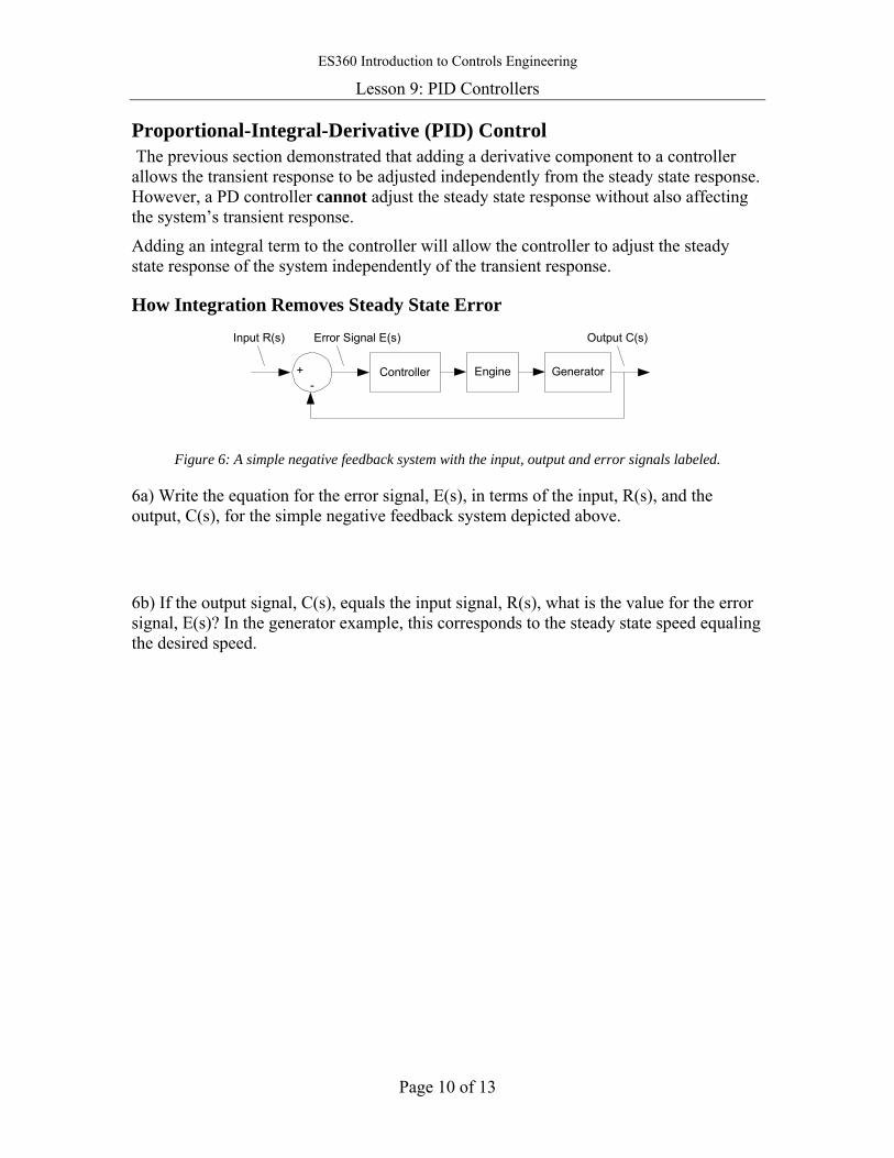
ES360 Introduction to Controls Engineering
Lesson 9: PID Controllers
Page 10 of 13
Proportional-Integral-Derivative (PID) Control The previous section demonstrated that adding a derivative component to a controller allows the transient response to be adjusted independently from the steady state response. However, a PD controller cannot adjust the steady state response without also affecting the system’s transient response.
Adding an integral term to the controller will allow the controller to adjust the steady state response of the system independently of the transient response.
How Integration Removes Steady State Error
Controller
Output C(s)Error Signal E(s)Input R(s)
-+ Engine Generator
Figure 6: A simple negative feedback system with the input, output and error signals labeled.
6a) Write the equation for the error signal, E(s), in terms of the input, R(s), and the output, C(s), for the simple negative feedback system depicted above.
6b) If the output signal, C(s), equals the input signal, R(s), what is the value for the error signal, E(s)? In the generator example, this corresponds to the steady state speed equaling the desired speed.
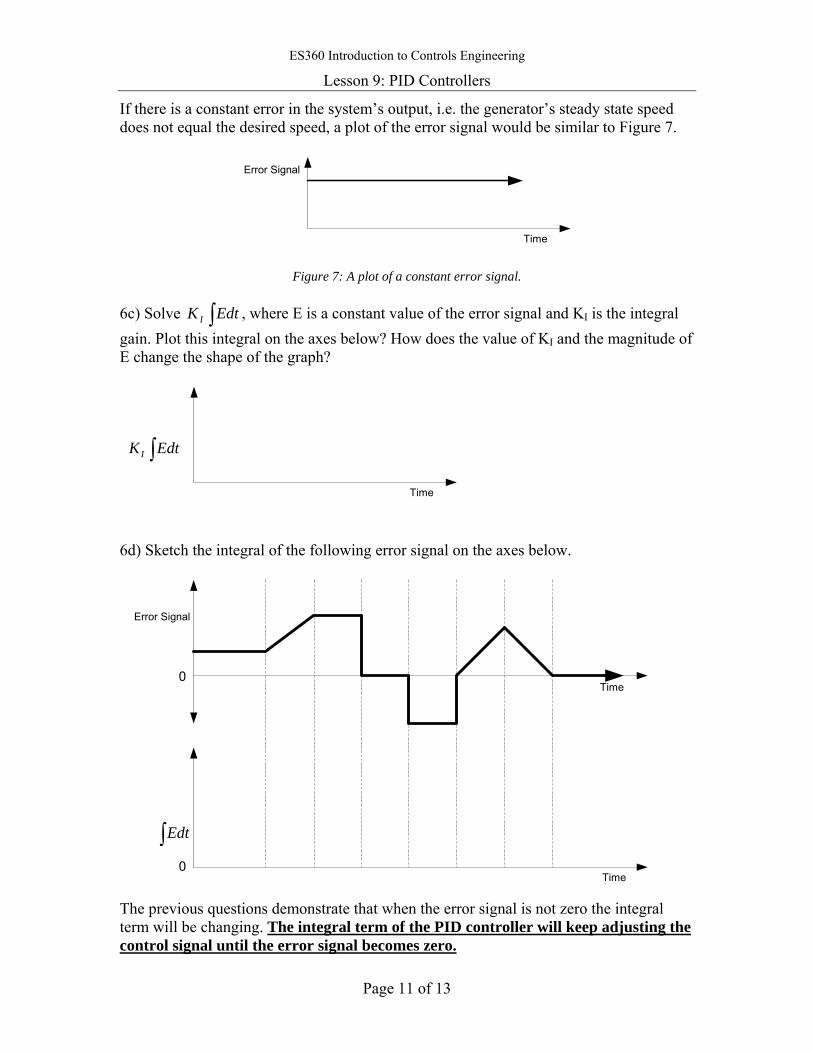
ES360 Introduction to Controls Engineering
Lesson 9: PID Controllers
Page 11 of 13
If there is a constant error in the system’s output, i.e. the generator’s steady state speed does not equal the desired speed, a plot of the error signal would be similar to Figure 7.
Time
Error Signal
Figure 7: A plot of a constant error signal.
6c) Solve ∫ EdtK I , where E is a constant value of the error signal and KI is the integral gain. Plot this integral on the axes below? How does the value of KI and the magnitude of E change the shape of the graph?
Time
∫ EdtKI
6d) Sketch the integral of the following error signal on the axes below.
Time
Error Signal
Time
∫ Edt
0
0
The previous questions demonstrate that when the error signal is not zero the integral term will be changing. The integral term of the PID controller will keep adjusting the control signal until the error signal becomes zero.
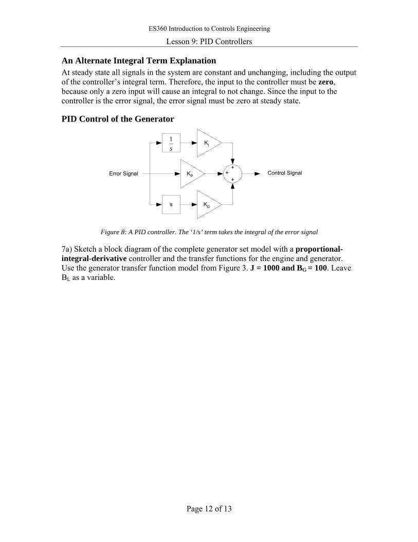
ES360 Introduction to Controls Engineering
Lesson 9: PID Controllers
Page 12 of 13
An Alternate Integral Term Explanation At steady state all signals in the system are constant and unchanging, including the output of the controller’s integral term. Therefore, the input to the controller must be zero, because only a zero input will cause an integral to not change. Since the input to the controller is the error signal, the error signal must be zero at steady state.
PID Control of the Generator
Control SignalError Signal KP+
+
KDs
KI
+
s1
Figure 8: A PID controller. The ‘1/s’ term takes the integral of the error signal
7a) Sketch a block diagram of the complete generator set model with a proportional-integral-derivative controller and the transfer functions for the engine and generator. Use the generator transfer function model from Figure 3. J = 1000 and BG = 100. Leave BL as a variable.
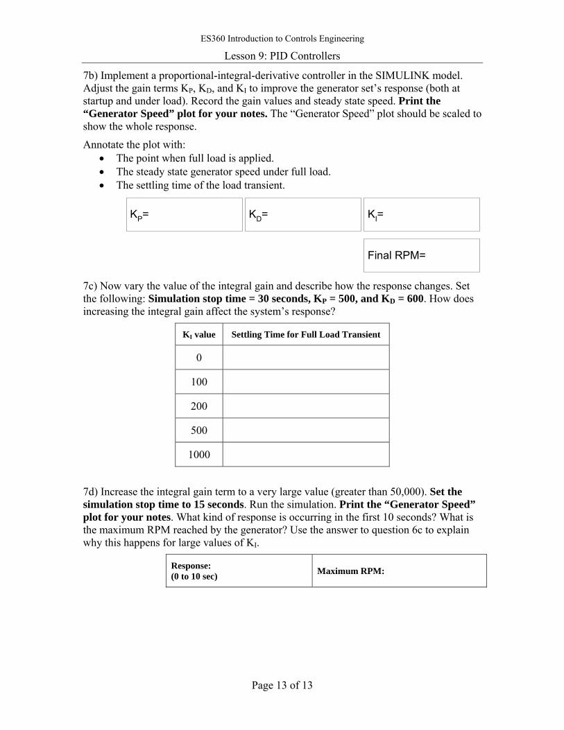
ES360 Introduction to Controls Engineering
Lesson 9: PID Controllers
Page 13 of 13
7b) Implement a proportional-integral-derivative controller in the SIMULINK model. Adjust the gain terms KP, KD, and KI to improve the generator set’s response (both at startup and under load). Record the gain values and steady state speed. Print the “Generator Speed” plot for your notes. The “Generator Speed” plot should be scaled to show the whole response.
Annotate the plot with: • The point when full load is applied. • The steady state generator speed under full load. • The settling time of the load transient.
KP= KD= KI=
Final RPM=
7c) Now vary the value of the integral gain and describe how the response changes. Set the following: Simulation stop time = 30 seconds, KP = 500, and KD = 600. How does increasing the integral gain affect the system’s response?
KI value Settling Time for Full Load Transient
0
100
200
500
1000
7d) Increase the integral gain term to a very large value (greater than 50,000). Set the simulation stop time to 15 seconds. Run the simulation. Print the “Generator Speed” plot for your notes. What kind of response is occurring in the first 10 seconds? What is the maximum RPM reached by the generator? Use the answer to question 6c to explain why this happens for large values of KI.
Response: (0 to 10 sec) Maximum RPM:


ES321L Introduction to Controls Engineering Name:
Lesson 10: PID Control and Discrete Sampling Section:
Page 1 of 16
Lesson 10: PID Control and Discrete Sampling
Part I: PID Control of the Cruise Missile’s Speed
Figure 1: The Tomahawk Land Attack Missile (TLAM), upper left. A Chinese YJ86LG, lower left. An Exocet impacting a target, right.
This lesson continues the exploration of a PID controller. For maximum strike effectiveness, a cruise missile’s “time on target” should be as close to the programmed value as possible. The PID controller will regulate the speed of a cruise missile to try to achieve the correct time on target. Typical parameters for a Tomahawk Land Attack Missile (TLAM) are listed in Table 1.
Simulation TLAM Parameters Maximum Speed 880 km/hr Minimum Speed 400 km/hr Maximum Range 1100 km
Table 1: TLAM Parameters
The mission profile can be graphed on a plot of distance vs. time. Initially (t=0) the missile is at the launch platform (d=0).
1a) What is the average speed required to reach a target 1000 km away in exactly 2 hours? Plot this mission profile on the axes below. How is speed depicted on this plot?
Time [hrs]
Dis
tanc
e [k
m]
Ave Speed =
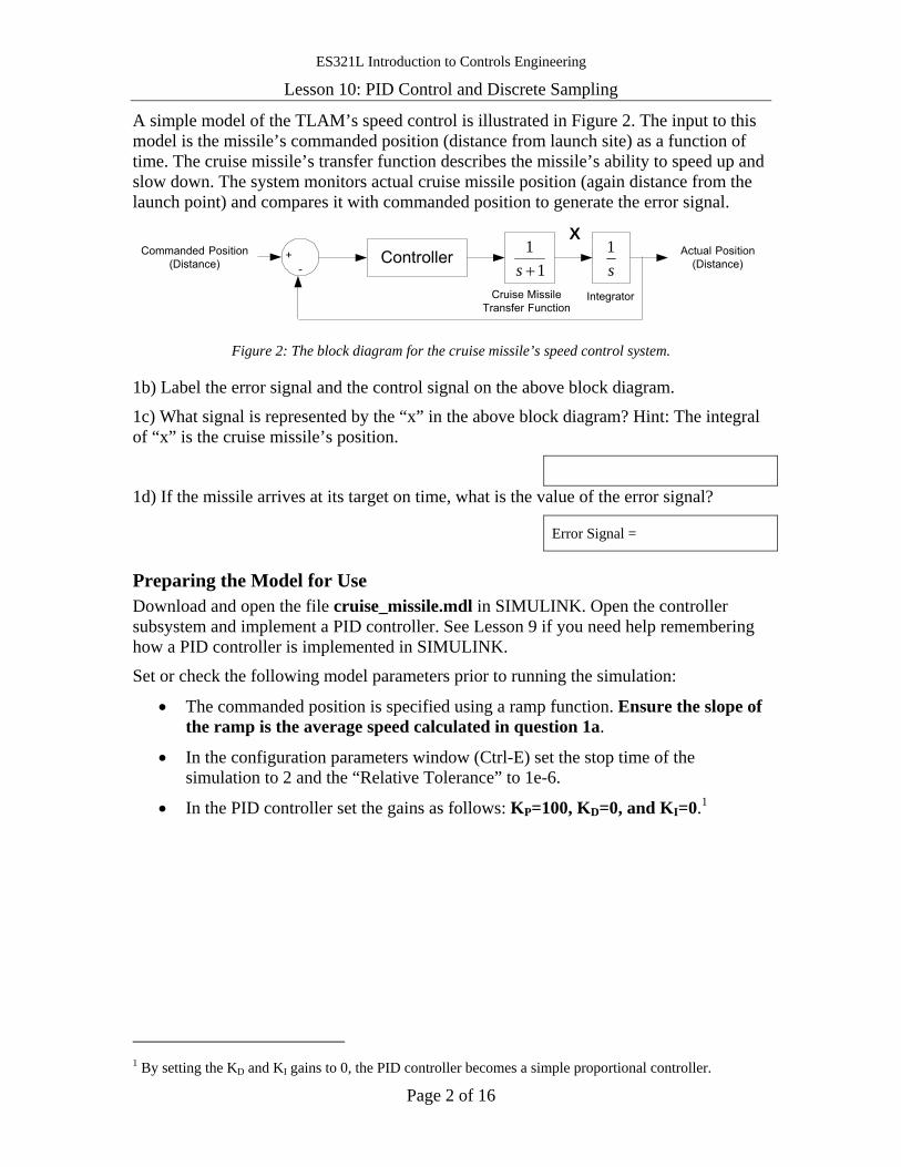
ES321L Introduction to Controls Engineering
Lesson 10: PID Control and Discrete Sampling
Page 2 of 16
A simple model of the TLAM’s speed control is illustrated in Figure 2. The input to this model is the missile’s commanded position (distance from launch site) as a function of time. The cruise missile’s transfer function describes the missile’s ability to speed up and slow down. The system monitors actual cruise missile position (again distance from the launch point) and compares it with commanded position to generate the error signal.
-+ Controller
s1
11+s
Cruise MissileTransfer Function
Integrator
XActual Position
(Distance)Commanded Position
(Distance)
Figure 2: The block diagram for the cruise missile’s speed control system.
1b) Label the error signal and the control signal on the above block diagram.
1c) What signal is represented by the “x” in the above block diagram? Hint: The integral of “x” is the cruise missile’s position.
1d) If the missile arrives at its target on time, what is the value of the error signal?
Error Signal =
Preparing the Model for Use Download and open the file cruise_missile.mdl in SIMULINK. Open the controller subsystem and implement a PID controller. See Lesson 9 if you need help remembering how a PID controller is implemented in SIMULINK.
Set or check the following model parameters prior to running the simulation:
• The commanded position is specified using a ramp function. Ensure the slope of the ramp is the average speed calculated in question 1a.
• In the configuration parameters window (Ctrl-E) set the stop time of the simulation to 2 and the “Relative Tolerance” to 1e-6.
• In the PID controller set the gains as follows: KP=100, KD=0, and KI=0.1
1 By setting the KD and KI gains to 0, the PID controller becomes a simple proportional controller.
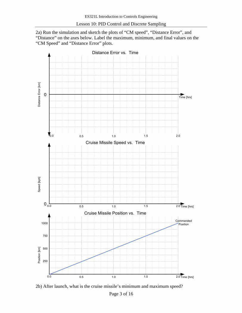
ES321L Introduction to Controls Engineering
Lesson 10: PID Control and Discrete Sampling
Page 3 of 16
2a) Run the simulation and sketch the plots of “CM speed”, “Distance Error”, and “Distance” on the axes below. Label the maximum, minimum, and final values on the “CM Speed” and “Distance Error” plots.
Dis
tanc
e E
rror
[km
]
Distance Error vs. Time
2.01.51.00.50.0
Time [hrs]0
Spe
ed [k
ph]
Cruise Missile Speed vs. Time
2.01.51.00.50.0 Time [hrs]0
Pos
ition
[km
]
Cruise Missile Position vs. Time
2.01.51.00.50.0 Time [hrs]
1000
500
750
250
CommandedPosition
2b) After launch, what is the cruise missile’s minimum and maximum speed?
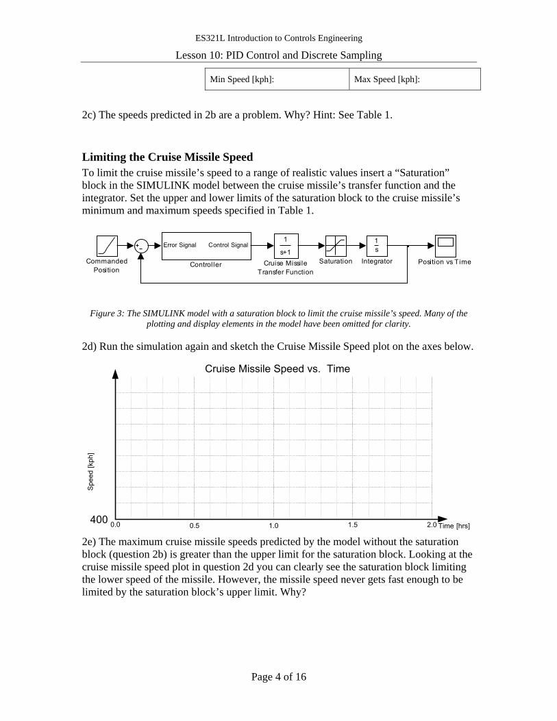
ES321L Introduction to Controls Engineering
Lesson 10: PID Control and Discrete Sampling
Page 4 of 16
Min Speed [kph]: Max Speed [kph]:
2c) The speeds predicted in 2b are a problem. Why? Hint: See Table 1.
Limiting the Cruise Missile Speed To limit the cruise missile’s speed to a range of realistic values insert a “Saturation” block in the SIMULINK model between the cruise missile’s transfer function and the integrator. Set the upper and lower limits of the saturation block to the cruise missile’s minimum and maximum speeds specified in Table 1.
Saturation Position vs Time
1s
Integrator
1
s+1Cruise Missile
Transfer Function
Error Signal Control Signal
ControllerCommandedPosition
Figure 3: The SIMULINK model with a saturation block to limit the cruise missile’s speed. Many of the
plotting and display elements in the model have been omitted for clarity.
2d) Run the simulation again and sketch the Cruise Missile Speed plot on the axes below.
Spe
ed [k
ph]
Cruise Missile Speed vs. Time
2.01.51.00.50.0 Time [hrs]400
2e) The maximum cruise missile speeds predicted by the model without the saturation block (question 2b) is greater than the upper limit for the saturation block. Looking at the cruise missile speed plot in question 2d you can clearly see the saturation block limiting the lower speed of the missile. However, the missile speed never gets fast enough to be limited by the saturation block’s upper limit. Why?
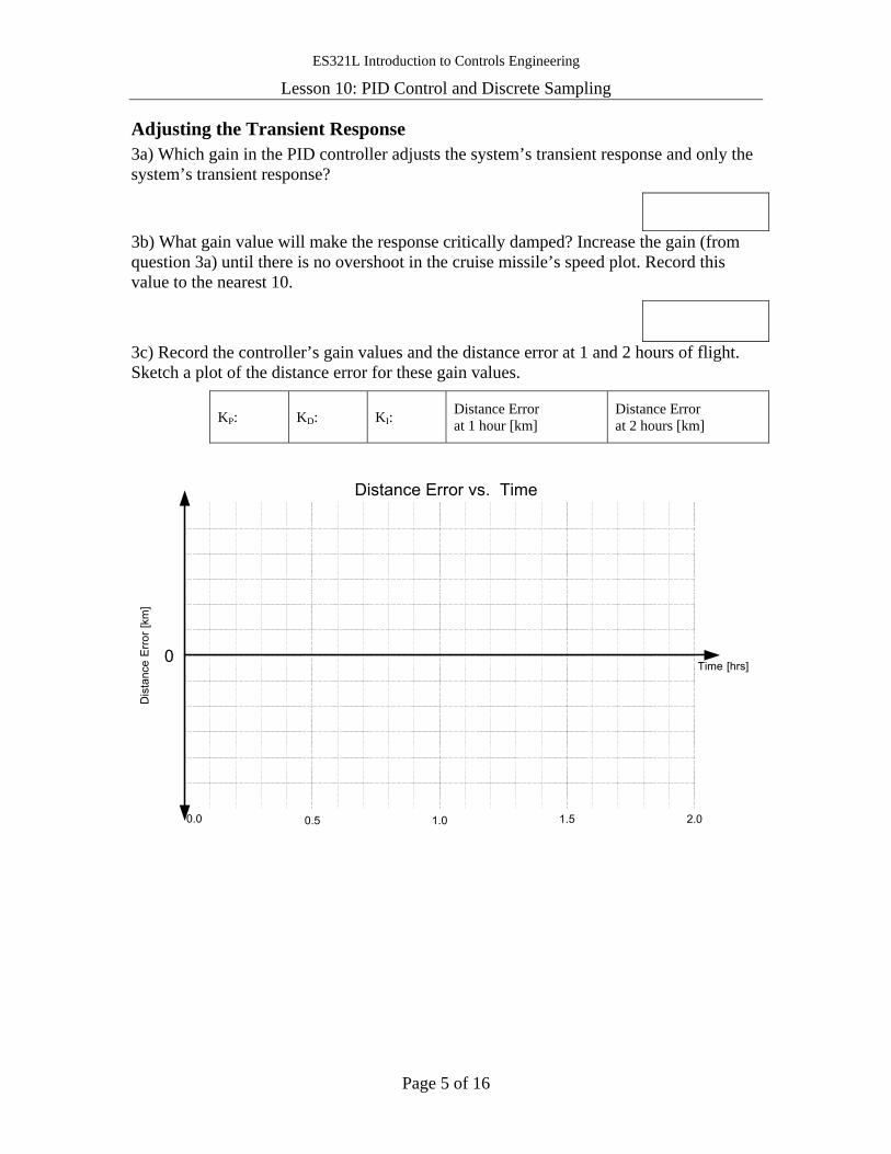
ES321L Introduction to Controls Engineering
Lesson 10: PID Control and Discrete Sampling
Page 5 of 16
Adjusting the Transient Response 3a) Which gain in the PID controller adjusts the system’s transient response and only the system’s transient response?
3b) What gain value will make the response critically damped? Increase the gain (from question 3a) until there is no overshoot in the cruise missile’s speed plot. Record this value to the nearest 10.
3c) Record the controller’s gain values and the distance error at 1 and 2 hours of flight. Sketch a plot of the distance error for these gain values.
KP: KD: KI: Distance Error at 1 hour [km]
Distance Error at 2 hours [km]
Dis
tanc
e E
rror [
km]
Distance Error vs. Time
2.01.51.00.50.0
Time [hrs]0
ES321L Introduction to Controls Engineering
Lesson 10: PID Control and Discrete Sampling
Page 6 of 16
Adjusting the Steady State Response 4a) Which gain term will adjust the system’s steady state value and only the system’s steady state value?
4b) Find the minimum value for this gain which minimizes the cruise missile’s distance error at 2 hrs. Record the gain value and the distance errors at 1 and 2 hours of flight. Sketch a plot of the distance error for these gain values.
KP: KD: KI: Distance Error at 1 hour [km]
Distance Error at 2 hours [km]
Dis
tanc
e E
rror [
km]
Distance Error vs. Time
2.01.51.00.50.0
Time [hrs]0
4c) Now try to also reduce the cruise missile’s distance error at 1 hour into flight. What happens to the distance error at 2 hours? Why?
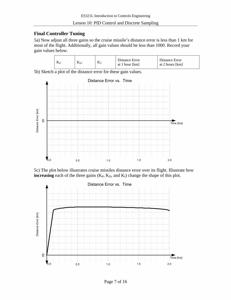
ES321L Introduction to Controls Engineering
Lesson 10: PID Control and Discrete Sampling
Page 7 of 16
Final Controller Tuning 5a) Now adjust all three gains so the cruise missile’s distance error is less than 1 km for most of the flight. Additionally, all gain values should be less than 1000. Record your gain values below.
KP: KD: KI: Distance Error at 1 hour [km]
Distance Error at 2 hours [km]
5b) Sketch a plot of the distance error for these gain values.
Dis
tanc
e E
rror [
km]
Distance Error vs. Time
2.01.51.00.50.0
Time [hrs]0
5c) The plot below illustrates cruise missiles distance error over its flight. Illustrate how increasing each of the three gains (KP, KD, and KI) change the shape of this plot.
Dis
tanc
e E
rror [
km]
Distance Error vs. Time
2.01.51.00.50.0
Time [hrs]0
ES321L Introduction to Controls Engineering
Lesson 10: PID Control and Discrete Sampling
Page 8 of 16
Part II: Discrete Sampling This section of the lesson will explore the differences between continuous and discrete sampling. In continuous sampling the feedback signal to the controller is always available and up to date at any and all instances of time. In discrete sampling the feedback signal to the controller is only updated periodically.
6a) Consider this simple example. When you are walking with your eyes open, you are receiving continuous feedback about your position with respect to objects around you. Now try walking around the room with your eyes closed, only open them once per second. How easy is it to walk quickly and avoid obstacles? How easy is it to run? Now try walking around the room again, this time only peek every 10 seconds. With your eyes closed longer, does this make it easier to move fast and avoid obstacles? Why or why not?
When you are walking with your eyes open your brain is a feedback system with continuous sampling. When walking with your eyes shut and only peeking occasionally, your brain is a feedback system with discrete sampling.
Discrete Sampling and the Cruise Missile The controller in the cruise missile needs a measurement of the missile’s current position to accurately fly the mission profile. A simple method of providing this position feedback is with a GPS receiver. However, most GPS receivers only provide position updates periodically (i.e. not continuously). This can be especially true in inclement weather or if obstacles are between the receiver and one or more of the satellites.
6b) How will the cruise missile’s performance change as the amount of time between position updates increases?
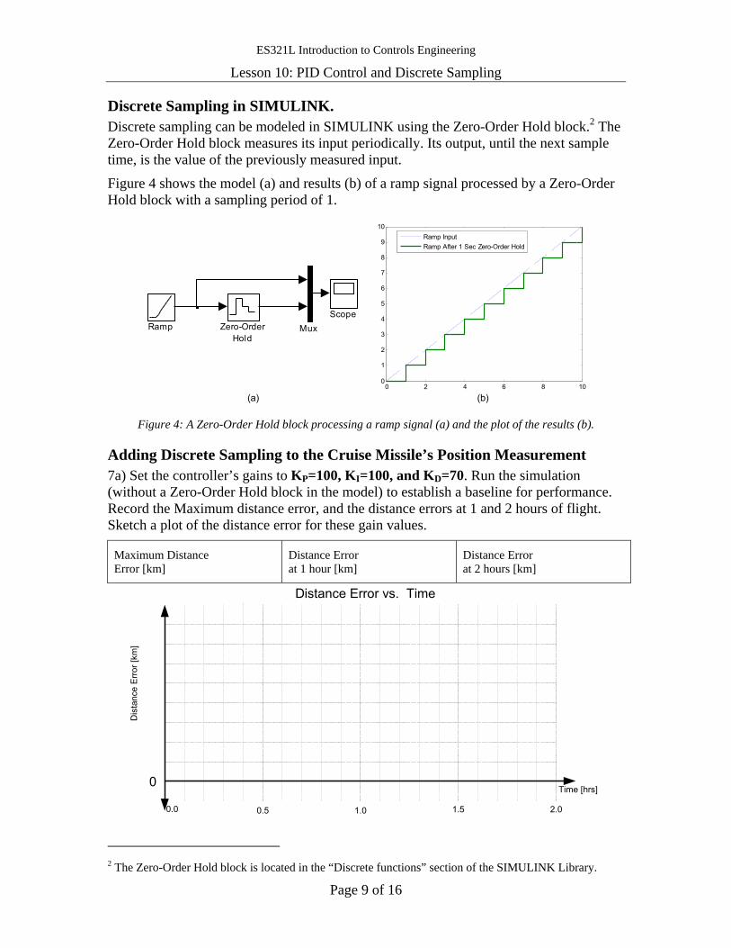
ES321L Introduction to Controls Engineering
Lesson 10: PID Control and Discrete Sampling
Page 9 of 16
Discrete Sampling in SIMULINK. Discrete sampling can be modeled in SIMULINK using the Zero-Order Hold block.2 The Zero-Order Hold block measures its input periodically. Its output, until the next sample time, is the value of the previously measured input.
Figure 4 shows the model (a) and results (b) of a ramp signal processed by a Zero-Order Hold block with a sampling period of 1.
MuxZero-OrderHold
ScopeRamp
0 2 4 6 8 100
1
2
3
4
5
6
7
8
9
10
Ramp InputRamp After 1 Sec Zero-Order Hold
(a) (b) Figure 4: A Zero-Order Hold block processing a ramp signal (a) and the plot of the results (b).
Adding Discrete Sampling to the Cruise Missile’s Position Measurement 7a) Set the controller’s gains to KP=100, KI=100, and KD=70. Run the simulation (without a Zero-Order Hold block in the model) to establish a baseline for performance. Record the Maximum distance error, and the distance errors at 1 and 2 hours of flight. Sketch a plot of the distance error for these gain values.
Maximum Distance Error [km]
Distance Error at 1 hour [km]
Distance Error at 2 hours [km]
Dis
tanc
e E
rror [
km]
Distance Error vs. Time
2.01.51.00.50.0
Time [hrs]0
2 The Zero-Order Hold block is located in the “Discrete functions” section of the SIMULINK Library.
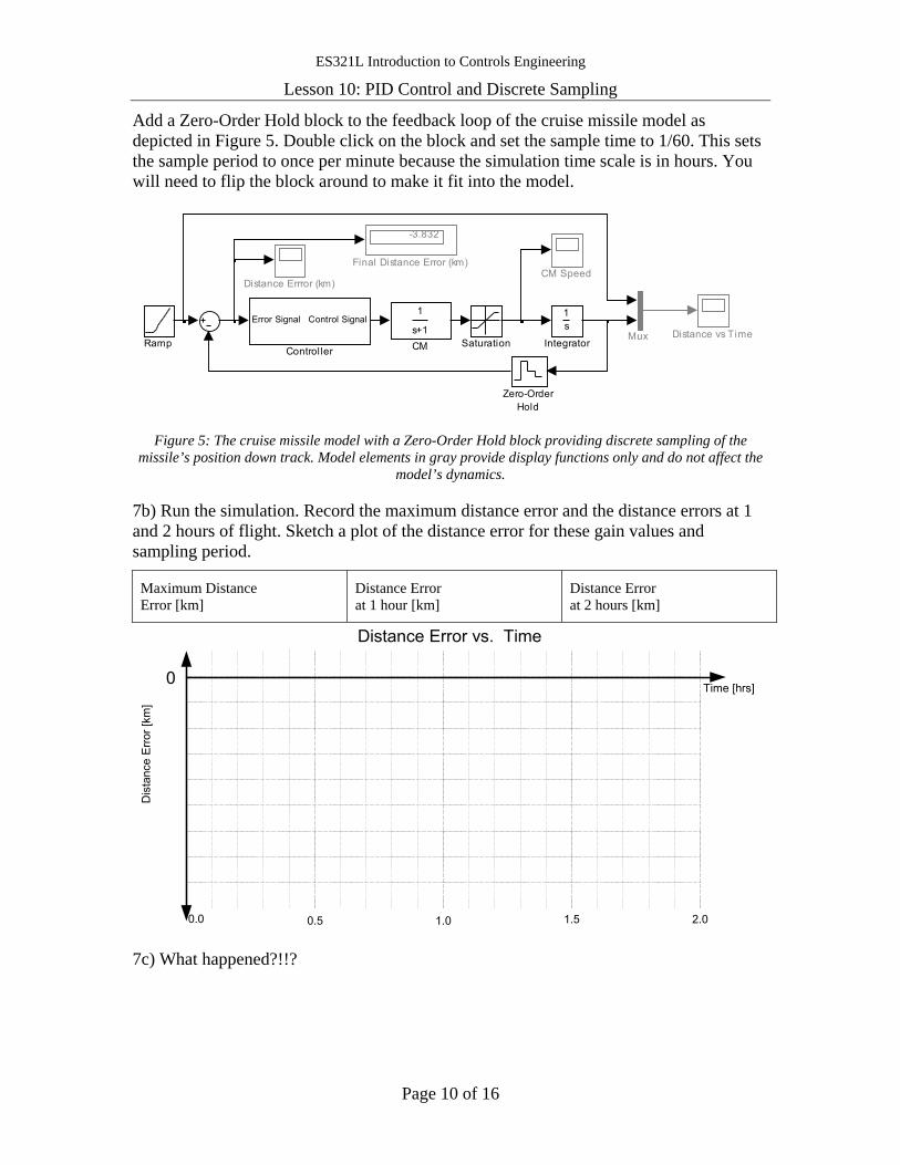
ES321L Introduction to Controls Engineering
Lesson 10: PID Control and Discrete Sampling
Page 10 of 16
Add a Zero-Order Hold block to the feedback loop of the cruise missile model as depicted in Figure 5. Double click on the block and set the sample time to 1/60. This sets the sample period to once per minute because the simulation time scale is in hours. You will need to flip the block around to make it fit into the model.
Mux
Zero-OrderHold
SaturationRamp
1s
Integrator
-3.832
Final Distance Error (km)
Distance vs Time
Distance Errror (km)
Error Signal Control Signal
Controller
CM Speed
1
s+1CM
Figure 5: The cruise missile model with a Zero-Order Hold block providing discrete sampling of the
missile’s position down track. Model elements in gray provide display functions only and do not affect the model’s dynamics.
7b) Run the simulation. Record the maximum distance error and the distance errors at 1 and 2 hours of flight. Sketch a plot of the distance error for these gain values and sampling period.
Maximum Distance Error [km]
Distance Error at 1 hour [km]
Distance Error at 2 hours [km]
Dis
tanc
e Er
ror [
km]
Distance Error vs. Time
2.01.51.00.50.0
Time [hrs]0
7c) What happened?!!?
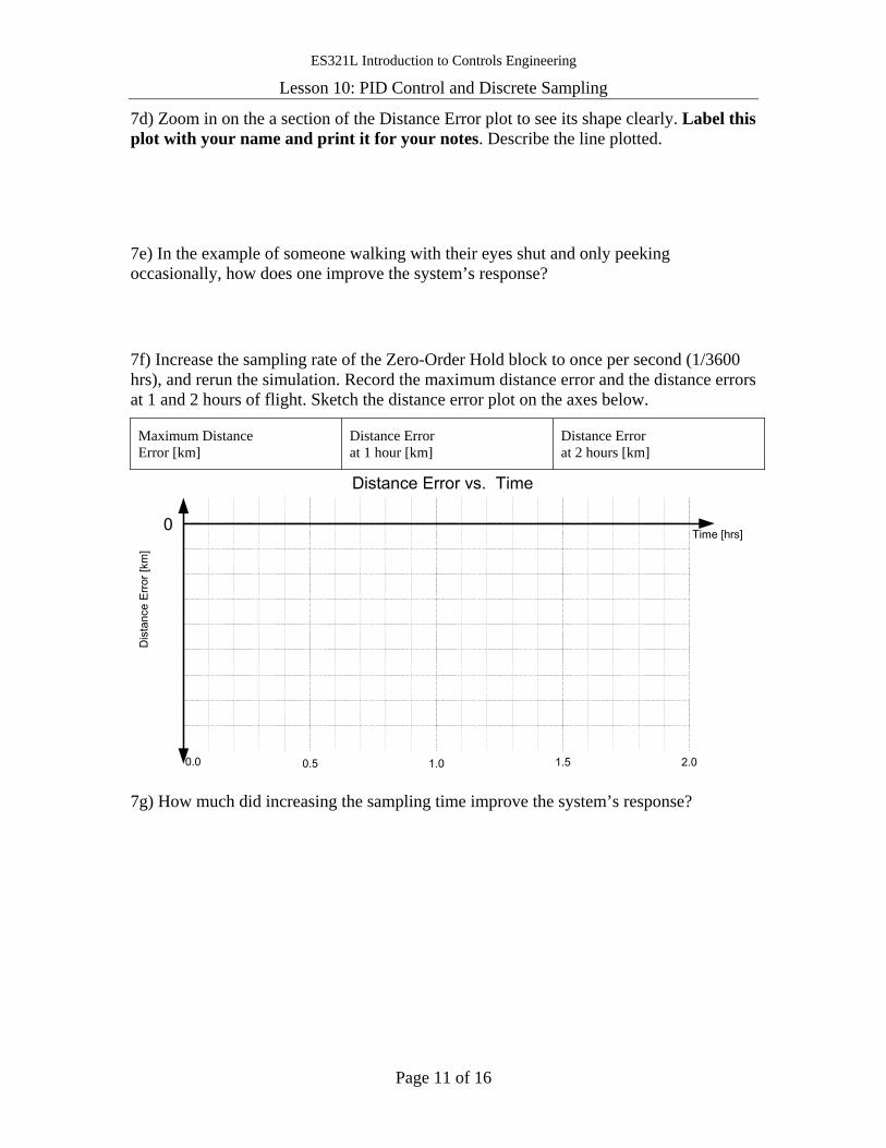
ES321L Introduction to Controls Engineering
Lesson 10: PID Control and Discrete Sampling
Page 11 of 16
7d) Zoom in on the a section of the Distance Error plot to see its shape clearly. Label this plot with your name and print it for your notes. Describe the line plotted.
7e) In the example of someone walking with their eyes shut and only peeking occasionally, how does one improve the system’s response?
7f) Increase the sampling rate of the Zero-Order Hold block to once per second (1/3600 hrs), and rerun the simulation. Record the maximum distance error and the distance errors at 1 and 2 hours of flight. Sketch the distance error plot on the axes below.
Maximum Distance Error [km]
Distance Error at 1 hour [km]
Distance Error at 2 hours [km]
Dis
tanc
e Er
ror [
km]
Distance Error vs. Time
2.01.51.00.50.0
Time [hrs]0
7g) How much did increasing the sampling time improve the system’s response?
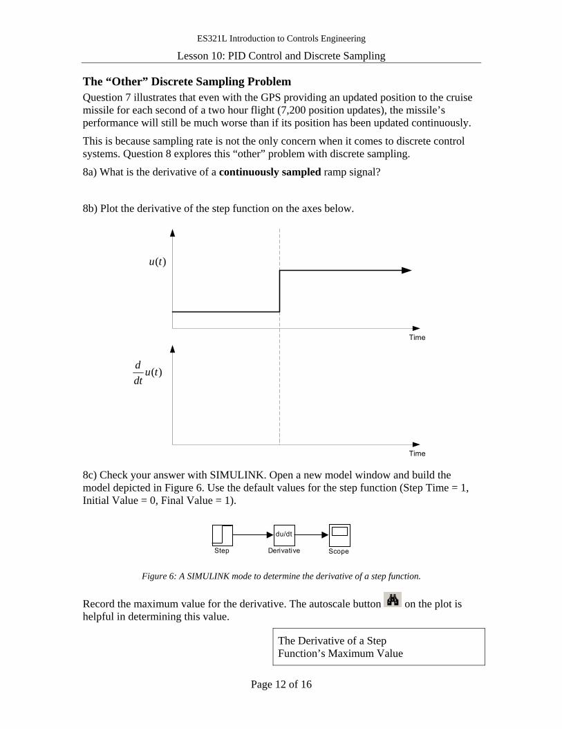
ES321L Introduction to Controls Engineering
Lesson 10: PID Control and Discrete Sampling
Page 12 of 16
The “Other” Discrete Sampling Problem Question 7 illustrates that even with the GPS providing an updated position to the cruise missile for each second of a two hour flight (7,200 position updates), the missile’s performance will still be much worse than if its position has been updated continuously.
This is because sampling rate is not the only concern when it comes to discrete control systems. Question 8 explores this “other” problem with discrete sampling.
8a) What is the derivative of a continuously sampled ramp signal?
8b) Plot the derivative of the step function on the axes below.
Time
Time
)(tu
)(tudtd
8c) Check your answer with SIMULINK. Open a new model window and build the model depicted in Figure 6. Use the default values for the step function (Step Time = 1, Initial Value = 0, Final Value = 1).
Step Scope
du/dt
Derivative
Figure 6: A SIMULINK mode to determine the derivative of a step function.
Record the maximum value for the derivative. The autoscale button on the plot is helpful in determining this value.
The Derivative of a Step Function’s Maximum Value
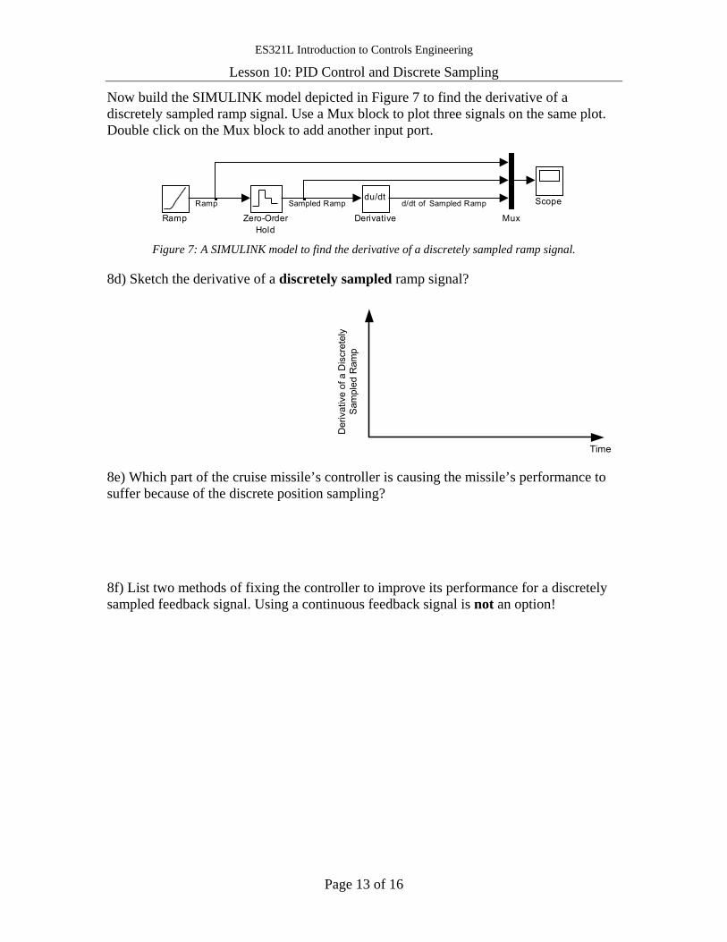
ES321L Introduction to Controls Engineering
Lesson 10: PID Control and Discrete Sampling
Page 13 of 16
Now build the SIMULINK model depicted in Figure 7 to find the derivative of a discretely sampled ramp signal. Use a Mux block to plot three signals on the same plot. Double click on the Mux block to add another input port.
MuxZero-OrderHold
Scope
Ramp
du/dt
Derivative
Sampled RampRamp d/dt of Sampled Ramp
Figure 7: A SIMULINK model to find the derivative of a discretely sampled ramp signal.
8d) Sketch the derivative of a discretely sampled ramp signal?
Time
Der
ivat
ive
of a
Dis
cret
ely
Sam
pled
Ram
p
8e) Which part of the cruise missile’s controller is causing the missile’s performance to suffer because of the discrete position sampling?
8f) List two methods of fixing the controller to improve its performance for a discretely sampled feedback signal. Using a continuous feedback signal is not an option!
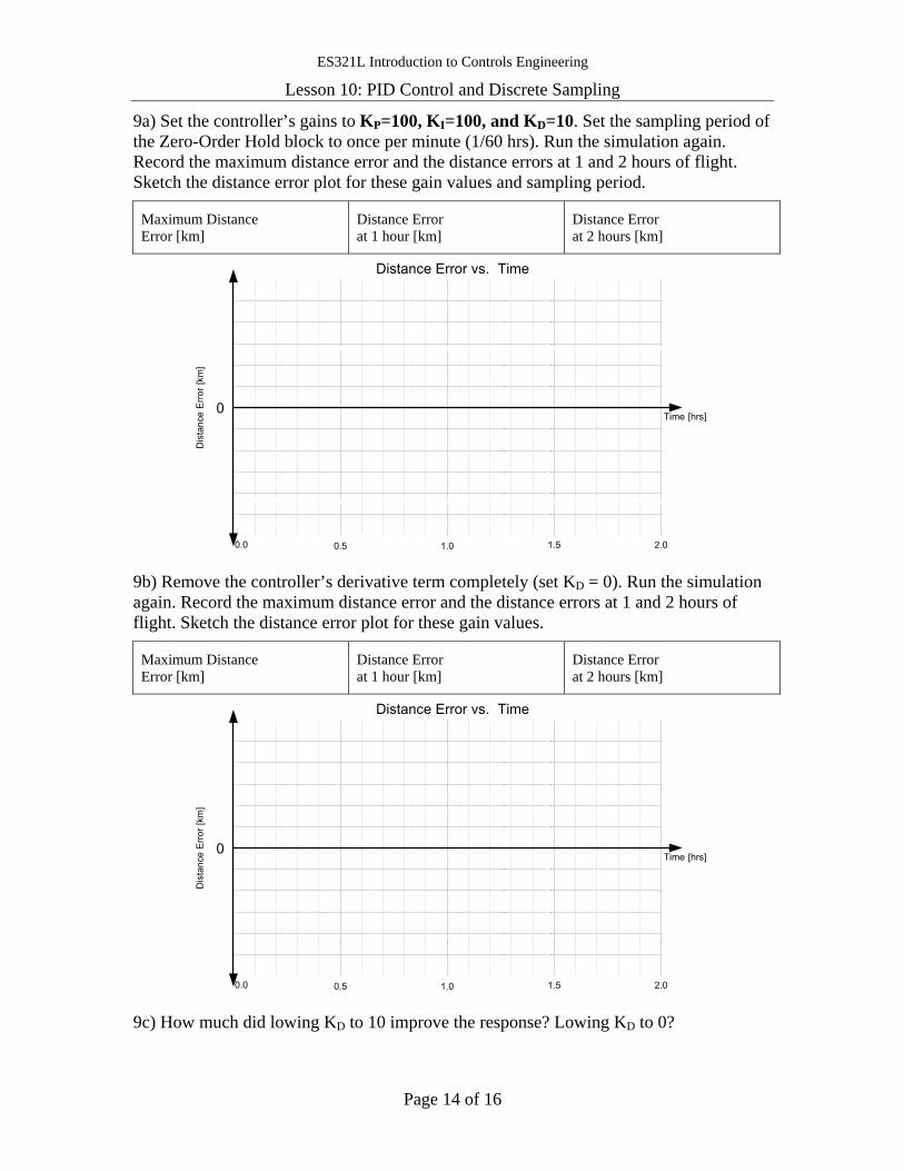
ES321L Introduction to Controls Engineering
Lesson 10: PID Control and Discrete Sampling
Page 14 of 16
9a) Set the controller’s gains to KP=100, KI=100, and KD=10. Set the sampling period of the Zero-Order Hold block to once per minute (1/60 hrs). Run the simulation again. Record the maximum distance error and the distance errors at 1 and 2 hours of flight. Sketch the distance error plot for these gain values and sampling period.
Maximum Distance Error [km]
Distance Error at 1 hour [km]
Distance Error at 2 hours [km]
Dis
tanc
e Er
ror [
km]
Distance Error vs. Time
2.01.51.00.50.0
Time [hrs]0
9b) Remove the controller’s derivative term completely (set KD = 0). Run the simulation again. Record the maximum distance error and the distance errors at 1 and 2 hours of flight. Sketch the distance error plot for these gain values.
Maximum Distance Error [km]
Distance Error at 1 hour [km]
Distance Error at 2 hours [km]
Dis
tanc
e E
rror [
km]
Distance Error vs. Time
2.01.51.00.50.0
Time [hrs]0
9c) How much did lowing KD to 10 improve the response? Lowing KD to 0?
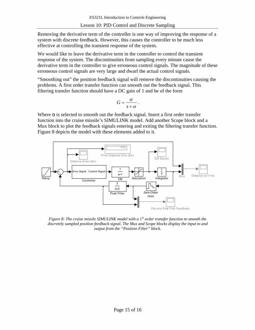
ES321L Introduction to Controls Engineering
Lesson 10: PID Control and Discrete Sampling
Page 15 of 16
Removing the derivative term of the controller is one way of improving the response of a system with discrete feedback. However, this causes the controller to be much less effective at controlling the transient response of the system.
We would like to leave the derivative term in the controller to control the transient response of the system. The discontinuities from sampling every minute cause the derivative term in the controller to give erroneous control signals. The magnitude of these erroneous control signals are very large and dwarf the actual control signals.
“Smoothing out” the position feedback signal will remove the discontinuities causing the problems. A first order transfer function can smooth out the feedback signal. This filtering transfer function should have a DC gain of 1 and be of the form
αα+
=s
G .
Where α is selected to smooth out the feedback signal. Insert a first order transfer function into the cruise missile’s SIMULINK model. Add another Scope block and a Mux block to plot the feedback signals entering and exiting the filtering transfer function. Figure 8 depicts the model with these elements added to it.
Mux
Zero-OrderHold
SaturationRamp
Pre and Post Filer Feedback
2
s+2Posit Fi lter
1s
Integrator
-123
Final Distance Error (km)
Distance vs Time
Distance Errror (km)
Error Signal Control Signal
Controller
CM Speed
1
s+1CM
Figure 8: The cruise missile SIMULINK model with a 1st order transfer function to smooth the
discretely sampled position feedback signal. The Mux and Scope blocks display the input to and output from the “Position Filter” block.

ES321L Introduction to Controls Engineering
Lesson 10: PID Control and Discrete Sampling
Page 16 of 16
10a) Set the sample time of the Zero-Order Hold block to once per minute (1/60 hrs). In Figure 8, α = 2. This value of α does not allow the filter’s output to accurately track its input. Run the simulation and adjust α so the position filter’s output closely tracts its input while at the same time smoothing its output. Record your value of α below.
α
Set all the controller gains to 100. Set the sample time of the Zero-Order Hold block to once per minute (1/60 hrs). 10b) Run the simulation again and print the “Cruise Missile Speed” and “Distance Error” plots for your notes. Label the plots with the gain values and sampling period. How is the cruise missile’s speed changing over the duration of the flight?
10c) Now set the sample time of the Zero-Order Hold block to once per second (1/3600 hrs). Run the simulation again and print the “Cruise Missile Speed” and “Distance Error” plots for your notes. Label the plots with the gain values and sampling period. How is the cruise missile’s speed changing over the duration of the flight?
10d) Has the faster sampling rate improved the cruise missile’s response?
10e) In this question, adjusting the sampling rate does affect the cruise missile’s response. In question 7, adjusting the sampling rate had little affect on the cruise missile’s response. Explain this difference in system behavior?
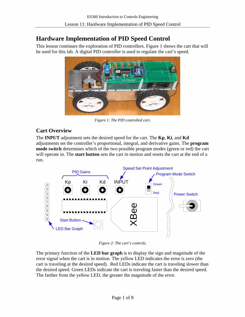
ES360 Introduction to Controls Engineering
Lesson 11: Hardware Implementation of PID Speed Control
Page 1 of 8
Hardware Implementation of PID Speed Control This lesson continues the exploration of PID controllers. Figure 1 shows the cart that will be used for this lab. A digital PID controller is used to regulate the cart’s speed.
Figure 1: The PID controlled cart.
Cart Overview The INPUT adjustment sets the desired speed for the cart. The Kp, Ki, and Kd adjustments set the controller’s proportional, integral, and derivative gains. The program mode switch determines which of the two possible program modes (green or red) the cart will operate in. The start button sets the cart in motion and resets the cart at the end of a run.
G
G
G
G
Y
R
R
R
R XB
ee
KdKp Ki INPUT
Start Button
LED Bar Graph
Program Mode Switch
Green
Red
PID GainsSpeed Set Point Adjustment
Power Switch
Figure 2: The cart’s controls.
The primary function of the LED bar graph is to display the sign and magnitude of the error signal when the cart is in motion. The yellow LED indicates the error is zero (the cart is traveling at the desired speed). Red LEDs indicate the cart is traveling slower than the desired speed. Green LEDs indicate the cart is traveling faster than the desired speed. The farther from the yellow LED, the greater the magnitude of the error.
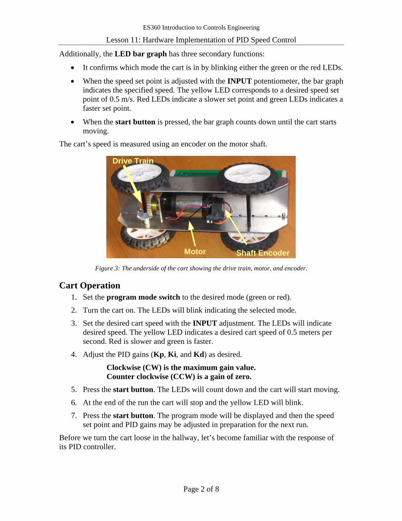
ES360 Introduction to Controls Engineering
Lesson 11: Hardware Implementation of PID Speed Control
Page 2 of 8
Additionally, the LED bar graph has three secondary functions:
• It confirms which mode the cart is in by blinking either the green or the red LEDs.
• When the speed set point is adjusted with the INPUT potentiometer, the bar graph indicates the specified speed. The yellow LED corresponds to a desired speed set point of 0.5 m/s. Red LEDs indicate a slower set point and green LEDs indicates a faster set point.
• When the start button is pressed, the bar graph counts down until the cart starts moving.
The cart’s speed is measured using an encoder on the motor shaft.
Shaft EncoderMotor
Drive Train
Figure 3: The underside of the cart showing the drive train, motor, and encoder.
Cart Operation 1. Set the program mode switch to the desired mode (green or red).
2. Turn the cart on. The LEDs will blink indicating the selected mode.
3. Set the desired cart speed with the INPUT adjustment. The LEDs will indicate desired speed. The yellow LED indicates a desired cart speed of 0.5 meters per second. Red is slower and green is faster.
4. Adjust the PID gains (Kp, Ki, and Kd) as desired.
Clockwise (CW) is the maximum gain value. Counter clockwise (CCW) is a gain of zero.
5. Press the start button. The LEDs will count down and the cart will start moving.
6. At the end of the run the cart will stop and the yellow LED will blink.
7. Press the start button. The program mode will be displayed and then the speed set point and PID gains may be adjusted in preparation for the next run.
Before we turn the cart loose in the hallway, let’s become familiar with the response of its PID controller.
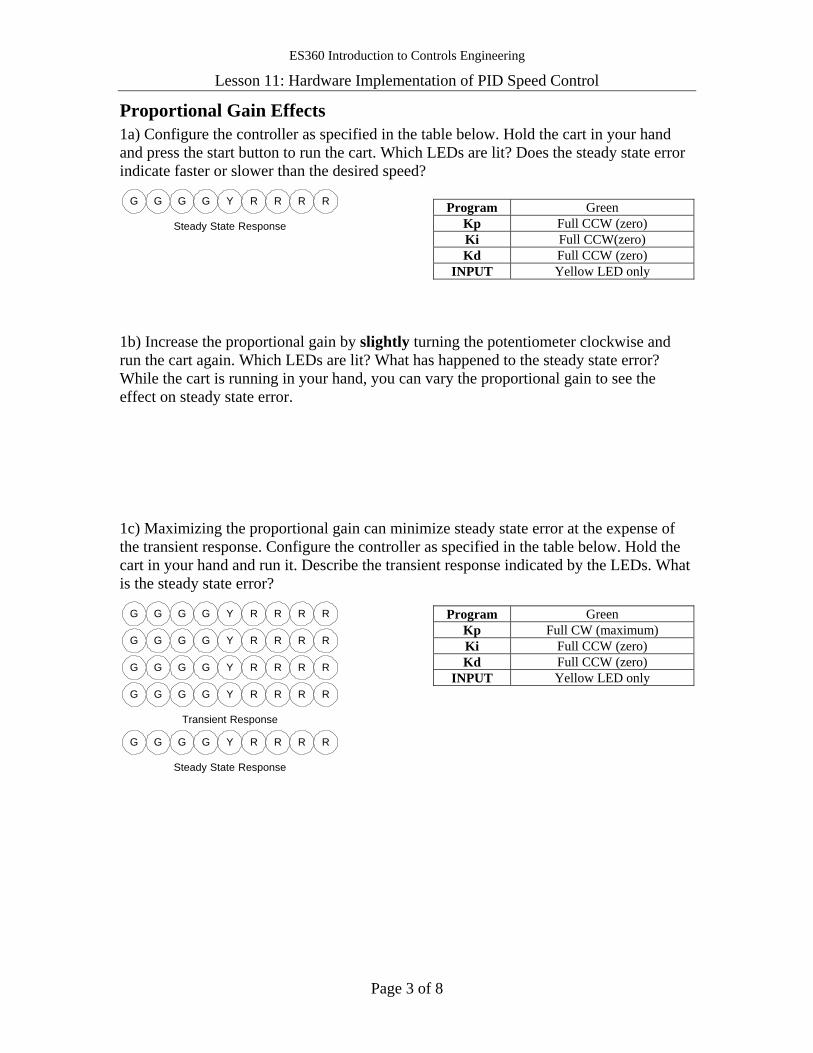
ES360 Introduction to Controls Engineering
Lesson 11: Hardware Implementation of PID Speed Control
Page 3 of 8
Proportional Gain Effects 1a) Configure the controller as specified in the table below. Hold the cart in your hand and press the start button to run the cart. Which LEDs are lit? Does the steady state error indicate faster or slower than the desired speed?
G G G G Y R R R R
Steady State Response
Program Green
Kp Full CCW (zero) Ki Full CCW(zero) Kd Full CCW (zero)
INPUT Yellow LED only
1b) Increase the proportional gain by slightly turning the potentiometer clockwise and run the cart again. Which LEDs are lit? What has happened to the steady state error? While the cart is running in your hand, you can vary the proportional gain to see the effect on steady state error.
1c) Maximizing the proportional gain can minimize steady state error at the expense of the transient response. Configure the controller as specified in the table below. Hold the cart in your hand and run it. Describe the transient response indicated by the LEDs. What is the steady state error?
G G G G Y R R R R
Transient Response
G G G G Y R R R R
G G G G Y R R R R
G G G G Y R R R R
G G G G Y R R R R
Steady State Response
Program Green
Kp Full CW (maximum) Ki Full CCW (zero) Kd Full CCW (zero)
INPUT Yellow LED only
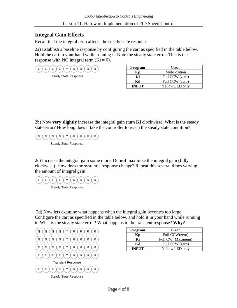
ES360 Introduction to Controls Engineering
Lesson 11: Hardware Implementation of PID Speed Control
Page 4 of 8
Integral Gain Effects Recall that the integral term affects the steady state response.
2a) Establish a baseline response by configuring the cart as specified in the table below. Hold the cart in your hand while running it. Note the steady state error. This is the response with NO integral term (Ki = 0).
G G G G Y R R R R
Steady State Response
Program Green Kp Mid-Position Ki Full CCW (zero) Kd Full CCW (zero)
INPUT Yellow LED only
2b) Now very slightly increase the integral gain (turn Ki clockwise). What is the steady state error? How long does it take the controller to reach the steady state condition?
G G G G Y R R R R
Steady State Response
2c) Increase the integral gain some more. Do not maximize the integral gain (fully clockwise). How does the system’s response change? Repeat this several times varying the amount of integral gain.
G G G G Y R R R R
Steady State Response
2d) Now lets examine what happens when the integral gain becomes too large. Configure the cart as specified in the table below, and hold it in your hand while running it. What is the steady state error? What happens to the transient response? Why?
G G G G Y R R R R
Transient Response
G G G G Y R R R R
G G G G Y R R R R
G G G G Y R R R R
G G G G Y R R R R
Steady State Response
Program Green Kp Full CCW(zero) Ki Full CW (Maximum) Kd Full CCW (zero)
INPUT Yellow LED only

ES360 Introduction to Controls Engineering
Lesson 11: Hardware Implementation of PID Speed Control
Page 5 of 8
Derivative Gain Effects Recall that the derivative gain affects only the transient response.
3a) Configure the cart to produce an under damped response by maximizing the proportional gain and setting the derivative and integral gains to zero specified in the table below. Hold it in your hand while running it. What is the largest oscillation of the error signal? What is the steady state error?
G G G G Y R R R R
Transient Response
G G G G Y R R R R
G G G G Y R R R R
G G G G Y R R R R
G G G G Y R R R R
Steady State Response
Program Green Kp Full CW (Maximum) Ki Full CCW (zero) Kd Full CCW (zero)
INPUT Yellow LED only
3b) Increase the derivative gain and run the cart again. Describe the transient response.
G G G G Y R R R R
Transient Response
G G G G Y R R R R
G G G G Y R R R R
G G G G Y R R R R
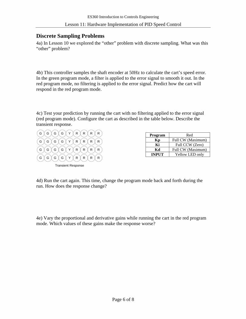
ES360 Introduction to Controls Engineering
Lesson 11: Hardware Implementation of PID Speed Control
Page 6 of 8
Discrete Sampling Problems 4a) In Lesson 10 we explored the “other” problem with discrete sampling. What was this “other” problem?
4b) This controller samples the shaft encoder at 50Hz to calculate the cart’s speed error. In the green program mode, a filter is applied to the error signal to smooth it out. In the red program mode, no filtering is applied to the error signal. Predict how the cart will respond in the red program mode.
4c) Test your prediction by running the cart with no filtering applied to the error signal (red program mode). Configure the cart as described in the table below. Describe the transient response.
G G G G Y R R R R
Transient Response
G G G G Y R R R R
G G G G Y R R R R
G G G G Y R R R R
Program Red
Kp Full CW (Maximum) Ki Full CCW (Zero) Kd Full CW (Maximum)
INPUT Yellow LED only
4d) Run the cart again. This time, change the program mode back and forth during the run. How does the response change?
4e) Vary the proportional and derivative gains while running the cart in the red program mode. Which values of these gains make the response worse?
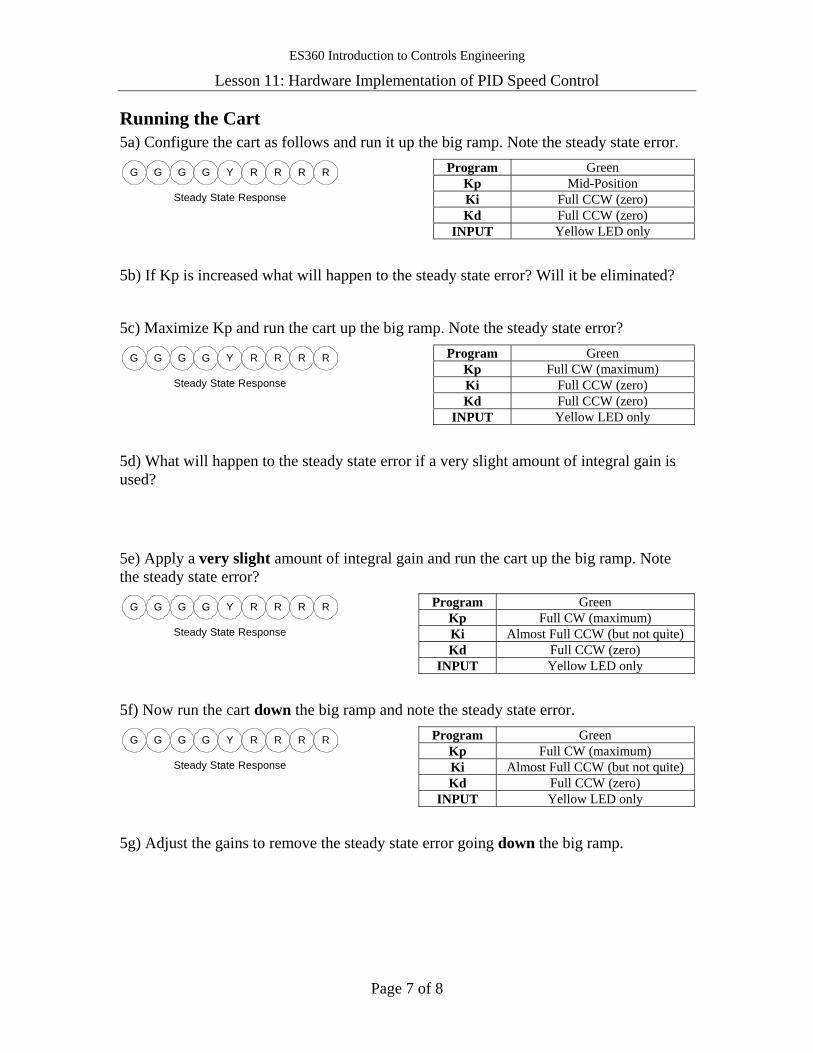
ES360 Introduction to Controls Engineering
Lesson 11: Hardware Implementation of PID Speed Control
Page 7 of 8
Running the Cart 5a) Configure the cart as follows and run it up the big ramp. Note the steady state error.
G G G G Y R R R R
Steady State Response
Program Green Kp Mid-Position Ki Full CCW (zero) Kd Full CCW (zero)
INPUT Yellow LED only
5b) If Kp is increased what will happen to the steady state error? Will it be eliminated?
5c) Maximize Kp and run the cart up the big ramp. Note the steady state error?
G G G G Y R R R R
Steady State Response
Program Green Kp Full CW (maximum) Ki Full CCW (zero) Kd Full CCW (zero)
INPUT Yellow LED only
5d) What will happen to the steady state error if a very slight amount of integral gain is used?
5e) Apply a very slight amount of integral gain and run the cart up the big ramp. Note the steady state error?
G G G G Y R R R R
Steady State Response
Program Green Kp Full CW (maximum) Ki Almost Full CCW (but not quite) Kd Full CCW (zero)
INPUT Yellow LED only
5f) Now run the cart down the big ramp and note the steady state error.
G G G G Y R R R R
Steady State Response
Program Green Kp Full CW (maximum) Ki Almost Full CCW (but not quite) Kd Full CCW (zero)
INPUT Yellow LED only
5g) Adjust the gains to remove the steady state error going down the big ramp.

ES360 Introduction to Controls Engineering
Lesson 11: Hardware Implementation of PID Speed Control
Page 8 of 8
5h) Were you able to remove the steady state error in question 5e? Why or why not?
5i) Add more friction to the cart by dragging a mass behind the cart as it runs down the ramp. Can you remove the steady state error now? Why or why not?
The cart is programmed to run a little over 5 meters. The goal is to have the cart run the 5 meter course in exactly 10 seconds. There are two 5 meter courses, one carpeted and one not carpeted. Run the cart several times on each. Adjust the gains to get the cart to run the course in exactly 10 seconds. You may use different gain settings for each course.
The cart should be run in the green program with the desired speed set to 0.5 meters per second (the yellow LED).
5j) Record your attempts in the table below. Course Speed Kp Ki Kd Time Comments
5k) For which course was it easier to have the cart meet the goal time? Why?