Efficient Algorithms for Mining Large Spatio-Temporal Data · 2020-01-17 · Efficient Algorithms...
198
Efficient Algorithms for Mining Large Spatio-Temporal Data Feng Chen Dissertation submitted to the faculty of the Virginia Polytechnic Institute and State University in partial fulfillment of the requirements for the degree of Doctor of Philosophy In Computer Science and Applications Chang-Tien Lu, Chair Ing Ray Chen Naren Ramakrishnan Wenjing Lou Yue Wang November 30, 2012 Falls Church, VA Keywords: Spatio-Temporal Analysis, Outlier Detection, Robust Prediction, Energy Disaggregation
Transcript of Efficient Algorithms for Mining Large Spatio-Temporal Data · 2020-01-17 · Efficient Algorithms...

Efficient Algorithms for Mining Large Spatio-Temporal Data
Feng Chen
Dissertation submitted to the faculty of the Virginia Polytechnic Institute and State University in
partial fulfillment of the requirements for the degree of
Doctor of Philosophy
In
Computer Science and Applications
Chang-Tien Lu, Chair
Ing Ray Chen
Naren Ramakrishnan
Wenjing Lou
Yue Wang
November 30, 2012
Falls Church, VA
Keywords: Spatio-Temporal Analysis, Outlier Detection, Robust Prediction, Energy
Disaggregation

Efficient Algorithms for Mining Large Spatio-Temporal Data
Feng Chen
ABSTRACT
Knowledge discovery on spatio-temporal datasets has attracted growing interests. Recent advances
on remote sensing technology mean that massive amounts of spatio-temporal data are being col-
lected, and its volume keeps increasing at an ever faster pace. It becomes critical to design efficient
algorithms for identifying novel and meaningful patterns from massive spatio-temporal datasets. Dif-
ferent from the other data sources, this data exhibits significant space-time statistical dependence,
and the assumption of i.i.d. is no longer valid. The exact modeling of space-time dependence will
render the exponential growth of model complexity as the data size increases. This research focuses
on the construction of efficient and effective approaches using approximate inference techniques for
three main mining tasks, including spatial outlier detection, robust spatio-temporal prediction, and
novel applications to real world problems.
Spatial novelty patterns, or spatial outliers, are those data points whose characteristics are markedly
different from their spatial neighbors. There are two major branches of spatial outlier detection
methodologies, which can be either global Kriging based or local Laplacian smoothing based. The
former approach requires the exact modeling of spatial dependence, which is time extensive; and the
latter approach requires the i.i.d. assumption of the smoothed observations, which is not statistically
solid. These two approaches are constrained to numerical data, but in real world applications we are
often faced with a variety of non-numerical data types, such as count, binary, nominal, and ordinal.
To summarize, the main research challenges are: 1) how much spatial dependence can be eliminated
via Laplace smoothing; 2) how to effectively and efficiently detect outliers for large numerical spatial
datasets; 3) how to generalize numerical detection methods and develop a unified outlier detection
framework suitable for large non-numerical datasets; 4) how to achieve accurate spatial prediction
even when the training data has been contaminated by outliers; 5) how to deal with spatio-temporal
data for the preceding problems.
To address the first and second challenges, we mathematically validated the effectiveness of Laplacian
smoothing on the elimination of spatial autocorrelations. This work provides fundamental support
for existing Laplacian smoothing based methods. We also discovered a nontrivial side-effect of
Laplacian smoothing, which ingests additional spatial variations to the data due to convolution
effects. To capture this extra variability, we proposed a generalized local statistical model, and
designed two fast forward and backward outlier detection methods that achieve a better balance
between computational efficiency and accuracy than most existing methods, and are well suited to
large numerical spatial datasets.
We addressed the third challenge by mapping non-numerical variables to latent numerical variables

iii
via a link function, such as logit function used in logistic regression, and then utilizing error-buffer
artificial variables, which follow a Student-t distribution, to capture the large valuations caused by
outliers. We proposed a unified statistical framework, which integrates the advantages of spatial
generalized linear mixed model, robust spatial linear model, reduced-rank dimension reduction, and
Bayesian hierarchical model. A linear-time approximate inference algorithm was designed to infer
the posterior distribution of the error-buffer artificial variables conditioned on observations. We
demonstrated that traditional numerical outlier detection methods can be directly applied to the
estimated artificial variables for outliers detection. To the best of our knowledge, this is the first
linear-time outlier detection algorithm that supports a variety of spatial attribute types, such as
binary, count, ordinal, and nominal.
To address the fourth and fifth challenges, we proposed a robust version of the Spatio-Temporal
Random Effects (STRE) model, namely the Robust STRE (R-STRE) model. The regular STRE
model is a recently proposed statistical model for large spatio-temporal data that has a linear
order time complexity, but is not best suited for non-Gaussian and contaminated datasets. This
deficiency can be systemically addressed by increasing the robustness of the model using heavy-
tailed distributions, such as the Huber, Laplace, or Student-t distribution to model the measurement
error, instead of the traditional Gaussian. However, the resulting R-STRE model becomes analytical
intractable, and direct application of approximate inferences techniques still has a cubic order time
complexity. To address the computational challenge, we reformulated the prediction problem as
a maximum a posterior (MAP) problem with a non-smooth objection function, transformed it to
a equivalent quadratic programming problem, and developed an efficient interior-point numerical
algorithm with a near linear order complexity. This work presents the first near linear time robust
prediction approach for large spatio-temporal datasets in both offline and online cases.

iv
Acknowledgements
First and foremost, I would like to thank my advisor, Dr. Chang-Tien Lu. Dr. Lu has contributed to
this work in many ways, and has taught me a tremendous amount. It was his energy and enthusiasm
that drew me to Virginia Tech, and led me down my current research path. Second, I would like
to thank my committee members, Dr. Ing Ray Chen, Dr. Naren Ramakrishnan, Dr. Wenjing Lou,
and Dr. Yue Wang; and my previous committee member Dr. Michael K. Badawy for many helpful
comments and insightful discussions from my proposal to final defense. Special thanks goes to Dr.
Wenjing Lou, who was willing to participate in my final defense committee at the last moment.
I would like to express appreciation to my friends in the Spatial Data Management Laboratory,
Xutong Liu, Yen-Cheng Lu, Bingsheng Wang, Haili Dong, Ting Hua, Liang Zhao, Kaiqun Fu, Manu
Shukla, Jing Dai, Ying Jin, Bing Liu, Arnold Boedijardjo, Edward Devilliers, Ray Dos Santos,
Wendell Jordan-Brangman, and Chad Steel. Many thanks for their precious comments on my
dissertation. Each discussion with them sparked new thoughts in my research. They made my
Ph.D. study an enjoyable journey with a lot of happy memory
Most importantly, I would like to thank my family and friends, for all of their love and support.

CONTENTS v
Contents
List of Figures x
List of Tables xi
1 Introduction 11.1 Research Issues . . . . . . . . . . . . . . . . . . . . . . . . . . . . . . . . . . . . . 3
1.1.1 Spatial Outlier Detection . . . . . . . . . . . . . . . . . . . . . . . . . . . . . . 3
1.1.2 Robust Spatio-Temporal Prediction . . . . . . . . . . . . . . . . . . . . . . . . 4
1.2 Contributions . . . . . . . . . . . . . . . . . . . . . . . . . . . . . . . . . . . . . . . 5
1.3 Proposal Organization . . . . . . . . . . . . . . . . . . . . . . . . . . . . . . . . . . 7
2 Theoretical Foundations and Related Works 92.1 Spatial Data Modeling . . . . . . . . . . . . . . . . . . . . . . . . . . . . . . . . . . 9
2.2 Laplacian Smoothing . . . . . . . . . . . . . . . . . . . . . . . . . . . . . . . . . . 14
2.3 Approximate Inference Techniques . . . . . . . . . . . . . . . . . . . . . . . . . . 16
2.4 Outlier Detection . . . . . . . . . . . . . . . . . . . . . . . . . . . . . . . . . . . . . 18
3 A Generalized Approach to Numerical Spatial Outlier Detec tion 213.1 Background and Motivation . . . . . . . . . . . . . . . . . . . . . . . . . . . . . . 22
3.2 Spatial Local Statistics and Related Works . . . . . . . . . . . . . . . . . . . . . 23
3.3 Generalized Local Spatial Statistics . . . . . . . . . . . . . . . . . . . . . . . . . . 24
3.3.1 Generalized Local Statistic Model (GLS) . . . . . . . . . . . . . . . . . . . . . 24
3.3.2 Theoretical Properties of GLS . . . . . . . . . . . . . . . . . . . . . . . . . . 26
3.4 Estimation and Inferences . . . . . . . . . . . . . . . . . . . . . . . . . . . . . . . 34
3.4.1 Generalized Least Squares Regression . . . . . . . . . . . . . . . . . . . . . . . 34
3.4.2 GLS-Backward Search Algorithm . . . . . . . . . . . . . . . . . . . . . . . . . 36
3.4.3 GLS-Forward Search Algorithm . . . . . . . . . . . . . . . . . . . . . . . . . . 37
3.4.4 Connections with Existing Methods . . . . . . . . . . . . . . . . . . . . . . . . 38
3.5 Simulations . . . . . . . . . . . . . . . . . . . . . . . . . . . . . . . . . . . . . . . . 40
3.5.1 Simulation Settings . . . . . . . . . . . . . . . . . . . . . . . . . . . . . . . . . 41
3.5.2 Detection Accuracy . . . . . . . . . . . . . . . . . . . . . . . . . . . . . . . . . 42
3.5.3 Computational Cost . . . . . . . . . . . . . . . . . . . . . . . . . . . . . . . . 43
3.5.4 Conclusion . . . . . . . . . . . . . . . . . . . . . . . . . . . . . . . . . . . . . 44

CONTENTS vi
4 A Generalized Approach to Non-Numerical Spatial Outlier D etection 464.1 Introduction . . . . . . . . . . . . . . . . . . . . . . . . . . . . . . . . . . . . . . . . 46
4.2 Theoretical Preliminaries . . . . . . . . . . . . . . . . . . . . . . . . . . . . . . . . 48
4.2.1 Reduced-Rank Spatial Linear (Gaussian Process) Model . . . . . . . . . . . . . 48
4.2.2 Spatial Generalized Linear Mixed Model (SGLMM) . . . . . . . . . . . . . . . . 49
4.3 Robust and Reduced-Rank Bayesian SGLMM model . . . . . . . . . . . . . . . . 50
4.3.1 The Observations Layer . . . . . . . . . . . . . . . . . . . . . . . . . . . . . . 50
4.3.2 The Latent Robust Gaussian process Layer . . . . . . . . . . . . . . . . . . . . 52
4.3.3 The Parameters Layer . . . . . . . . . . . . . . . . . . . . . . . . . . . . . . . 52
4.3.4 Theoretical Interpretation . . . . . . . . . . . . . . . . . . . . . . . . . . . . . 53
4.4 Robust Approximate Inference . . . . . . . . . . . . . . . . . . . . . . . . . . . . . 53
4.4.1 Inference on Latent variables . . . . . . . . . . . . . . . . . . . . . . . . . . . . 54
4.4.2 Inference on Parameters . . . . . . . . . . . . . . . . . . . . . . . . . . . . . . 55
4.4.3 Non-Numerical Spatial Outlier Detection . . . . . . . . . . . . . . . . . . . . . 55
4.4.4 Time and Space Complexity Analysis . . . . . . . . . . . . . . . . . . . . . . . 57
4.5 Experiments . . . . . . . . . . . . . . . . . . . . . . . . . . . . . . . . . . . . . . . . 58
4.5.1 Experiment Settings . . . . . . . . . . . . . . . . . . . . . . . . . . . . . . . . 58
4.5.2 Detection Effectiveness . . . . . . . . . . . . . . . . . . . . . . . . . . . . . . . 63
4.5.3 Detection Efficiency . . . . . . . . . . . . . . . . . . . . . . . . . . . . . . . . 66
4.5.4 Impact of Model Parameters . . . . . . . . . . . . . . . . . . . . . . . . . . . . 67
4.6 Conclusion . . . . . . . . . . . . . . . . . . . . . . . . . . . . . . . . . . . . . . . . 67
5 Robust Prediction for Large Spatio-Temporal Data Sets 695.1 Introduction . . . . . . . . . . . . . . . . . . . . . . . . . . . . . . . . . . . . . . . . 70
5.2 Theoretical Preliminaries . . . . . . . . . . . . . . . . . . . . . . . . . . . . . . . . 72
5.2.1 Spatio-Temporal Random Effects Model . . . . . . . . . . . . . . . . . . . . . . 72
5.2.2 Fixed Rank Spatio-Temporal Prediction . . . . . . . . . . . . . . . . . . . . . . 73
5.3 Problem Formulation . . . . . . . . . . . . . . . . . . . . . . . . . . . . . . . . . . 73
5.3.1 Robust Spatio-Temporal Random Effects Model . . . . . . . . . . . . . . . . . 74
5.3.2 Problem Formulation . . . . . . . . . . . . . . . . . . . . . . . . . . . . . . . . 74
5.4 A General Approach . . . . . . . . . . . . . . . . . . . . . . . . . . . . . . . . . . . 75
5.4.1 MAP Estimation of η1:T |T , ξ1:T |T . . . . . . . . . . . . . . . . . . . . . . . . 76
5.4.2 LA Estimation of the Precision Matrix G1:T |T . . . . . . . . . . . . . . . . . . 77
5.5 Optimization Techniques . . . . . . . . . . . . . . . . . . . . . . . . . . . . . . . . 79
5.5.1 Primal-Dual Optimization for Huber Distribution . . . . . . . . . . . . . . . . . 79
5.5.2 Primal-Dual Optimization for Laplace Distribution . . . . . . . . . . . . . . . . 82
5.5.3 Time and Space Complexity Analysis . . . . . . . . . . . . . . . . . . . . . . . 83
5.6 Experiments . . . . . . . . . . . . . . . . . . . . . . . . . . . . . . . . . . . . . . . . 83
5.6.1 Simulation Study . . . . . . . . . . . . . . . . . . . . . . . . . . . . . . . . . . 84
5.6.2 Experiments on Aerosol Optical Depth Data . . . . . . . . . . . . . . . . . . . 87
5.6.3 Experiments on Traffic Volume Data . . . . . . . . . . . . . . . . . . . . . . . 88

CONTENTS vii
6 Application 1: Activity Analysis Based on Low Sample Rate S mart Me-ters 956.1 Introduction . . . . . . . . . . . . . . . . . . . . . . . . . . . . . . . . . . . . . . . . 96
6.2 Background . . . . . . . . . . . . . . . . . . . . . . . . . . . . . . . . . . . . . . . . 97
6.2.1 Problem and Definition . . . . . . . . . . . . . . . . . . . . . . . . . . . . . . . 99
6.2.2 Research Challenges . . . . . . . . . . . . . . . . . . . . . . . . . . . . . . . . 99
6.2.3 Observations . . . . . . . . . . . . . . . . . . . . . . . . . . . . . . . . . . . . 100
6.3 A NEW STATISTICAL DISAGGREGATION FRAMEWORK . . . . . . . . . . . . . 101
6.4 DISAGGREGATION APPROACHES . . . . . . . . . . . . . . . . . . . . . . . . . . 103
6.4.1 HMM-based Approach . . . . . . . . . . . . . . . . . . . . . . . . . . . . . . . 104
6.4.2 Classification-GMM-based Approach . . . . . . . . . . . . . . . . . . . . . . . . 107
6.5 Evaluation & Findings . . . . . . . . . . . . . . . . . . . . . . . . . . . . . . . . . . 109
6.5.1 Datasets . . . . . . . . . . . . . . . . . . . . . . . . . . . . . . . . . . . . . . 109
6.5.2 Parameter Settings & Baseline Methods . . . . . . . . . . . . . . . . . . . . . . 110
6.5.3 Effectiveness Comparison . . . . . . . . . . . . . . . . . . . . . . . . . . . . . . 111
6.5.4 Impact of Sample Rate . . . . . . . . . . . . . . . . . . . . . . . . . . . . . . . 113
6.5.5 Disaggregation for Pilot Households . . . . . . . . . . . . . . . . . . . . . . . . 113
6.6 Related Work . . . . . . . . . . . . . . . . . . . . . . . . . . . . . . . . . . . . . . . 116
7 Application 2: Wireless Passive Device Fingerprinting us ing InfiniteHidden Markov Random Field 1187.1 Introduction . . . . . . . . . . . . . . . . . . . . . . . . . . . . . . . . . . . . . . . . 119
7.2 Related Work . . . . . . . . . . . . . . . . . . . . . . . . . . . . . . . . . . . . . . . 121
7.2.1 Radio-metric Based Device Fingerprinting . . . . . . . . . . . . . . . . . . . . . 121
7.2.2 RSS Based Device Fingerprinting . . . . . . . . . . . . . . . . . . . . . . . . . 121
7.3 Features for Device Fingerprinting . . . . . . . . . . . . . . . . . . . . . . . . . . 122
7.3.1 Time Measurement . . . . . . . . . . . . . . . . . . . . . . . . . . . . . . . . . 123
7.3.2 Frequency Measurement . . . . . . . . . . . . . . . . . . . . . . . . . . . . . . 123
7.3.3 Phase Shift Difference Measurement . . . . . . . . . . . . . . . . . . . . . . . 124
7.3.4 Angle of Arrival Measurement . . . . . . . . . . . . . . . . . . . . . . . . . . . 125
7.3.5 Radio Signal Strength (RSS) Measurement . . . . . . . . . . . . . . . . . . . . 125
7.4 Problem Formulation . . . . . . . . . . . . . . . . . . . . . . . . . . . . . . . . . . 127
7.5 Theoretical Backgrounds . . . . . . . . . . . . . . . . . . . . . . . . . . . . . . . . 128
7.5.1 Hidden Markov Random Field . . . . . . . . . . . . . . . . . . . . . . . . . . . 128
7.5.2 Infinite Gaussian Mixture Model . . . . . . . . . . . . . . . . . . . . . . . . . . 129
7.6 Infinite Hidden Markov Random Field (iHMRF) . . . . . . . . . . . . . . . . . . . 130
7.7 Incremental Variational Inference for the IHMRF Model . . . . . . . . . . . . . . 132
7.7.1 Model Building Phase . . . . . . . . . . . . . . . . . . . . . . . . . . . . . . . 134
7.7.2 Compression Phase . . . . . . . . . . . . . . . . . . . . . . . . . . . . . . . . . 135
7.7.3 Incremental Batch Update Phase . . . . . . . . . . . . . . . . . . . . . . . . . 136
7.8 Simulation Result . . . . . . . . . . . . . . . . . . . . . . . . . . . . . . . . . . . . 136

CONTENTS viii
7.8.1 Simulation Setup . . . . . . . . . . . . . . . . . . . . . . . . . . . . . . . . . . 137
7.8.2 Impacts of Instable RSS Collection Rates . . . . . . . . . . . . . . . . . . . . . 140
7.8.3 Impacts of Transmission Power Changes . . . . . . . . . . . . . . . . . . . . . 141
7.8.4 Comparisons on Precision, Recall, and F-Measure . . . . . . . . . . . . . . . . . 141
7.8.5 Comparison on Time Costs . . . . . . . . . . . . . . . . . . . . . . . . . . . . . 142
7.8.6 A Case Study on Detecting Masquerade Attacks . . . . . . . . . . . . . . . . . 142
7.9 Conclusion . . . . . . . . . . . . . . . . . . . . . . . . . . . . . . . . . . . . . . . . 143
8 Achievements and Future Work 1478.1 Achievements . . . . . . . . . . . . . . . . . . . . . . . . . . . . . . . . . . . . . . . 147
8.2 Future Work . . . . . . . . . . . . . . . . . . . . . . . . . . . . . . . . . . . . . . . . 151
8.2.1 Spatial and Spatio-Temporal Outlier Detection . . . . . . . . . . . . . . . . . . 151
8.2.2 Spatio-Temporal Anomalous Cluster Detection . . . . . . . . . . . . . . . . . . 152
8.2.3 Energy Disaggregation . . . . . . . . . . . . . . . . . . . . . . . . . . . . . . . 152
8.2.4 Wireless Device Fingerprinting . . . . . . . . . . . . . . . . . . . . . . . . . . . 153
8.3 Published Papers . . . . . . . . . . . . . . . . . . . . . . . . . . . . . . . . . . . . . 154
A Appendix 157A.1 Estimated Bound . . . . . . . . . . . . . . . . . . . . . . . . . . . . . . . . . . . . . 157
A.2 Definition of Matrices M and E . . . . . . . . . . . . . . . . . . . . . . . . . . . . 157
A.3 Proof of Theorem 2 . . . . . . . . . . . . . . . . . . . . . . . . . . . . . . . . . . . 160
A.4 Proof of Theorem 3 . . . . . . . . . . . . . . . . . . . . . . . . . . . . . . . . . . . 162
A.5 Offline Inference Solution for iHMRF . . . . . . . . . . . . . . . . . . . . . . . . . 163
Bibliography 164

LIST OF FIGURES ix
List of Figures
3.1 An example of correlation: it reflects the noise and direction of a linear relationship . . 29
3.2 The neighborhoods defined by 4 or 12-nearest-neighbors rules in gridded data, equal to
those defined by radiuses r and 2r . . . . . . . . . . . . . . . . . . . . . . . . . . . . . 31
3.3 Comparison on computational cost (setting: linear trend, isolated outliers, α = 0.1, σ20 =
2, c = 15,K = 8, n = 200) . . . . . . . . . . . . . . . . . . . . . . . . . . . . . . . . . 44
3.4 Outlier ROC Curve Comparison (the same setting: n = 200, b = 5, σ2C = 20) . . . . . 45
4.1 Graphic Model Representation of the 3RB-SGLMM Model . . . . . . . . . . . . . . . . 51
4.2 Spatial Distribution of Four Simulation Datasets . . . . . . . . . . . . . . . . . . . . . 60
4.3 Spatial Distribution of Six Real Life Datasets . . . . . . . . . . . . . . . . . . . . . . . 61
4.4 Spatial Distribution of Simulation Data . . . . . . . . . . . . . . . . . . . . . . . . . . 64
4.5 Detection Rate Comparison on Four Real Datasets . . . . . . . . . . . . . . . . . . . . 65
4.6 Time Cost Analysis . . . . . . . . . . . . . . . . . . . . . . . . . . . . . . . . . . . . . 66
4.7 Detection Rate Comparison Using Different Knot Sizes . . . . . . . . . . . . . . . . . . 67
5.1 pdfs of Heavy Tailed Distributions . . . . . . . . . . . . . . . . . . . . . . . . . . . . . 75
5.2 Approximations of Heavy Tailed Distributions . . . . . . . . . . . . . . . . . . . . . . . 78
5.3 Experiment Design . . . . . . . . . . . . . . . . . . . . . . . . . . . . . . . . . . . . . 84
5.4 Comparison between the FR-STP and RFR-STP using the data observed at four different
times and with different numbers of isolated outliers (15 unobserved locations from s =
113 to s = 127) . . . . . . . . . . . . . . . . . . . . . . . . . . . . . . . . . . . . . . . 92
5.5 Comparison between the FR-STP and RFR-STP using the data observed at two different
times and with different sizes of regional outliers (15 unobserved locations from s = 113
to s = 127) . . . . . . . . . . . . . . . . . . . . . . . . . . . . . . . . . . . . . . . . . 93
5.6 Comparison between the FR-STP and RFR-STP on the contaminated AOD data sets
observed at time t = 5 . . . . . . . . . . . . . . . . . . . . . . . . . . . . . . . . . . . 93
5.7 Comparison between the FR-STP and RFR-STP using the Traffic Volume Data on the
4th day. (Detectors #75 and #215 are spatial neighbors) . . . . . . . . . . . . . . . . . 94
6.1 An Example of Data and Disaggregated Activities . . . . . . . . . . . . . . . . . . . . 97
6.2 Data Acquisition . . . . . . . . . . . . . . . . . . . . . . . . . . . . . . . . . . . . . . 98
6.3 Smarter Water Service Architecture . . . . . . . . . . . . . . . . . . . . . . . . . . . . 99
6.4 Disaggregation Framework . . . . . . . . . . . . . . . . . . . . . . . . . . . . . . . . . 102
6.5 Impact of Interval Length . . . . . . . . . . . . . . . . . . . . . . . . . . . . . . . . . 113

LIST OF FIGURES x
6.6 Distribution vs. Demographic Info . . . . . . . . . . . . . . . . . . . . . . . . . . . . . 114
6.7 Washer Usage vs. Day of Week . . . . . . . . . . . . . . . . . . . . . . . . . . . . . . 115
6.8 Shower vs. Day of Week . . . . . . . . . . . . . . . . . . . . . . . . . . . . . . . . . . 115
6.9 Shower/Washer vs. Time of Day . . . . . . . . . . . . . . . . . . . . . . . . . . . . . . 116
7.1 Illustration of phase shift difference for constellation of QPSK symbols of two transmitters 124
7.2 Features extraction from packets . . . . . . . . . . . . . . . . . . . . . . . . . . . . . . 127
7.3 Graphical Model Representation of iGMM . . . . . . . . . . . . . . . . . . . . . . . . . 130
7.4 Graphical Model Representation of iHMRF . . . . . . . . . . . . . . . . . . . . . . . . 132
7.5 Spatial Distribution of Simulation Data . . . . . . . . . . . . . . . . . . . . . . . . . . 138
7.6 Comparison on Time Costs (Seconds) . . . . . . . . . . . . . . . . . . . . . . . . . . 142
7.7 Visualization for the UdelModels Data with 1 Building 10 Floors . . . . . . . . . . . . . 144
7.8 Visualization for the UdelModels - Chicago9B1k Data with Pedestrians and Cars . . . 145
7.9 Visualization for the UdelModels - Chicago9B1k Data with Only Cars . . . . . . . . . . 146
A.1 The comparison between the true correlation |ρ(ω∗i , ω
∗j ;θθθ)| and the estimated bound
function. Here, K = 12, c = 6. . . . . . . . . . . . . . . . . . . . . . . . . . . . . . . . 158
A.2 The comparison between the true correlation |ρ(ω∗i , ω
∗j ;θθθ)| and the estimated bound
function. Here, K = 12,c = 11. . . . . . . . . . . . . . . . . . . . . . . . . . . . . . . . 158
A.3 The comparison between the true correlation |ρ(ω∗i , ω
∗j ;θθθ)| and the estimated bound
function. Here, K = 12,c = 15. . . . . . . . . . . . . . . . . . . . . . . . . . . . . . . . 159
A.4 The comparison between the true correlation |ρ(ω∗i , ω
∗j ;θθθ)| and the estimated bound
function. Here, K = 12,c = 20. . . . . . . . . . . . . . . . . . . . . . . . . . . . . . . . 159
A.5 The comparison between the true correlation |ρ(ω∗i , ω
∗j ;θθθ)| and the estimated bound
function. Here, K = 12,c = 40. . . . . . . . . . . . . . . . . . . . . . . . . . . . . . . . 160

LIST OF TABLES xi
List of Tables
3.1 Description of major symbols . . . . . . . . . . . . . . . . . . . . . . . . . . . . . . . . 24
3.2 Combination of parameter settings . . . . . . . . . . . . . . . . . . . . . . . . . . . . . 42
3.3 Competition statistics for different combinations of parameter settings . . . . . . . . . 43
4.1 Simulation Model Settings . . . . . . . . . . . . . . . . . . . . . . . . . . . . . . . . . 59
4.2 Real life Data Settings . . . . . . . . . . . . . . . . . . . . . . . . . . . . . . . . . . . 62
5.1 Comparison of Time Cost using the Simulated and AOD Data (Seconds) . . . . . . . . 91
5.2 Comparison of Robustness using the AOD data . . . . . . . . . . . . . . . . . . . . . . 91
6.1 Terms & Definitions . . . . . . . . . . . . . . . . . . . . . . . . . . . . . . . . . . . . 100
6.2 Water Journaling of One Household . . . . . . . . . . . . . . . . . . . . . . . . . . . . 110
6.3 Precision, Recall, and F-measure on Simulation Data . . . . . . . . . . . . . . . . . . . 112
6.4 Precision, Recall, and F-measure on Volunteers . . . . . . . . . . . . . . . . . . . . . . 113
7.1 Device Fingerprinting Features . . . . . . . . . . . . . . . . . . . . . . . . . . . . . . . 125
7.2 Definition of TP, FP, FN, and TN . . . . . . . . . . . . . . . . . . . . . . . . . . . . . 137
7.3 Simulation Data Settings . . . . . . . . . . . . . . . . . . . . . . . . . . . . . . . . . . 137
7.4 Simulation Results Based on UdelModels with 1 Building 10 Floors . . . . . . . . . . . 139
7.5 Simulation Results Based on UdelModels - Chicago9Blk - with Pedestrians and Cars . . 139
7.6 Simulation Results Based on UdelModels - Chicago9Blk - with Only Cars . . . . . . . . 139
7.7 Simulation Results Based on UdelModels - Chicago9Blk - with Only Pedestrians . . . . 140
7.8 Unstable RSS Rates (UdelModels - Chicago9Blk - with Only Pedestrians) . . . . . . . 141
7.9 Change of Transmission Power (UdelModels - Chicago9Blk - with Only Pedestrians) . . 141
7.10 Detection Rates for Masquerade Attacks Based on UdelModels - Chicago9B1k - Pedestrains
143
7.11 Detection Rates for Masquerade Attacks on UdelModels - Chicago9B1k - 1 Building 10
Floors . . . . . . . . . . . . . . . . . . . . . . . . . . . . . . . . . . . . . . . . . . . . 143

Chapter 1 1
Chapter 1
Introduction
In recent years, with the advancements of remote sensoring techniques and the widespread use of
mobile devices, such as GPS and intelligent phones, the amount of spatial (or geographic) data have
been multiplied. The ever-increasing volume of spatial data has greatly challenged our ability to
store, retrieve, and extract useful but implicit knowledge from them. This is crucial for many ap-
plication domains including ecology and environmental management, public safety, transportation,
earth science, epidemiology, and climatology [4]. A number of research works have been conducted
to develop the Spatial Data Management System (SDBMS). The major research areas on spa-
tial databases include spatial data modeling, spatial data access, spatial data query, spatial data
visualization, and spatial data mining (or knowledge discovery).
Spatial data mining [285,224,264,263] is the process of discovering previously unknown and poten-
tially useful patterns from large spatial data sets. Similar to traditional data mining, spatial data
mining techniques can be categorized into clustering, classification, co-location mining, and outlier
detection [4]. However, traditional data mining may not be directly applied to mine spatial data
because of the complexity of spatial data, intrinsic spatial relationships, and spatial autocorrelations.
By the first law of geography, “Everything is related to everything else, but nearby things are more
related than distant things” [55].
In many applications, especially in sensor networks, the spatial data are continuously collected and
the addition of temporal information to spatial data makes the mining of spatial patterns even more
challenging. It is crucial to consider both spatial and temporal dependency during the knowledge
discovery process. To process temporal and streaming data, a number of work has been conducted
on the modelling [36], querying [42, 240, 244], classification [252, 230, 289, 291], clustering [245], as
well as visualization [210].
This research focuses on the development of local space and geometry based techniques for three
spatial mining tasks, including spatial outlier detection, anomalous cluster detection, and spatial
classification. These tasks have a wide array of applications. Some of them are described as follows.

Chapter 1 2
In this following chapters, we use “anomaly detection” to denote both the first two tasks.
• Event detection in sensor networks. Nowadays, sensor networks [214,5,6] have attracted
increasing attentions and many sensor networks are in the deployment process, such as habitat
monitoring applications [29], smart grid [30], and IBM smarter planet [31] projects. There are
a variety of sensor networks applications where anomaly detection is central. Typical examples
include: (1) environment monitoring, in which anomaly detection can identify when and where
an event occurs based on the regional temperature and humidity information collected by
sensors [27]; (2) habitat monitoring, in which sensors are equipped on endangered species to
monitor their daily life, and anomaly detection can indicate their abnormal behaviors [26]; (3)
health and medical monitoring, in which different portions of patients are equipped with sensors
and anomaly detection can indicate potential diseases [28]; (4) industry monitoring, in which
anomaly detection can detect possible malfunctions and other abnormalities by equipping
the temperature, pressure, and vibration amplitude sensors in the machines [29]; (5) target
tracking, in which the moving targets can by tracked by equipping GPS sensors and anomaly
detection can filter erroneous information and improve the tracking accuracy and efficiency [7,
8]; (6) detection of traffic incidents and traffic congestions [56, 286]; and (7) detection of
radioactive, biological or chemical materials [10, 9, 11].
• Object detection in digital images. The literature on the detection of spatial objects
in images has been several decades, mainly focused on the fields of satellite imagery [12–15],
computer vision [16, 17], and medical imaging [18–21]. One of its most recent applications is
within the brain imaging domain. Spatial anomalous cluster detection has been applied to
indicate brain regions that have been affected by some diseases, such as stroke or degenerative
diseases [78]. It has also been applied to identify brain regions that correlate to some brain
activities. For example, it is possible to tell wether a person is watching a movie or reading a
book by monitoring the functional magnetic resonance imaging (FMRI) images of their brain
activities [80].
• Disease Outbreak Surveillance. Disease surveillance is one of the major application do-
mains for spatial anomalous cluster detection. It is of great practical utility to detect the
emerging of disease outbreaks as early as possible. The presence of chemical and biological
pollutions in some geographic regions can also be detected indirectly if these materials have
impacts on human health [22–24].
• Intrusion and virus detection in a computer network. With the widespread use of
internet technologies, computers can be easily affected by virus or worms spreading through
a computer network [25]. The slightly abnormal symptoms (e.g., slight loss of performance
and presence of system instability) presented in infected computers could be difficult to be
detected on a single machine.

1.1 Research Issues 3
1.1 Research Issues
This research aims to investigate and develop local based efficient and effective learning techniques
for spatio-temporal data. The major research issues are stated as follows:
1.1.1 Spatial Outlier Detection
Spatial outlier detection aims to find a small group of data objects that deviate significantly from the
rest large amount of data, by considering the effects of spatial autocorrelations. Existing solutions
for spatial outlier detection can be categorized into two branches, including global and local based
detection methods. Global based methods were designed based on the robust estimation of global
statistical models (e.g., ordinary or universal Kriging models). For this category, outlier detection
can be regarded a by-product of the robust estimation of a prediction model. However there are
applications where outlier detection is central, rather than prediction. It may be important and
more efficient to identify outliers without being able to estimate the complete model. This is the
major motivation for local based detection methods. The basic idea of local based methods is
to first calculate the local difference (or Laplacian-smoothed value) for each object, which is the
difference between the non-spatial attribute of the object and the aggregated value (e.g., average)
of its spatial neighbors. By assuming i.i.d. normal distributions for these local differences, the local
based approach discovers outlier objects by robust estimation of the related local model parameters,
such as the aggregated values, mean, and standard deviation. There are four major issues that this
research addresses for spatial outlier detection.
1. Statistical foundations for local based methods. Existing local based detection methods
have the advantages of simplicity and high efficiency. These methods were designed based on
the fundamental assumption that the calculated local differences are i.i.d. normal. However,
no justifications for this assumption have ever been proposed. It is important to study the
situations where this assumption is appropriate and where it is inappropriate. The appropri-
ateness can be measured by a statistical significance level, e.g., at 0.5% level. A variety of
scenarios need to be tested, which can be modeled by different statistical frameworks (e.g., or-
dinary and universal kriging) under different parameter settings. Example parameters include
different data structures (e.g., continuous space, lattice space, and transportation network),
neighborhood definitions (e.g., defined by K nearest neighbors or by Voronoi), neighborhood
size, and covariance models (e.g., spherical, exponential, and gaussian kernels).
2. Accuracy and performance parametrization. There exist popular situations where the
assumption of i.i.d normal is violated. In these situations the performances of existing local
based detection methods deteriorate significantly. There are four major scenarios to be consid-
ered. First, some data may exhibit linear or nonlinear global trend, which can be represented by
some parametric forms, such as polynomial of spatial locations or linear combinations of other
basis functions (e.g., Gaussian basis functions). Second, the local (or Laplacian) smoothing
1.1.2 Robust Spatio-Temporal Prediction 4
process by calculating local differences can help reduce spatial autocorrelations between data
objects. However this smoothing process will also increase correlations between data objects
because of the convolution effect [54]. Third, some spatial data may have different regional
characteristics, such as population density, community types, and spatial heterogeneities, e.g.,
two cities separated by a mountain range. These regional features will lead to varying auto-
correlations across different regions. Fourth, some spatial data may exhibit a complex trend
structure that can not be described by some parametric form. In this case, nonparametric
estimation techniques need to be considered.
3. Comparisons between local and global based methods. Rare research works have been
published to compare the performance between local and global based methods theoretically
and empirically. From the theoretical side, the key is to identify the situations where the spatial
autocorrelations between objects can not be removed significantly (e.g., 0.05 level) by local (or
Laplacian) smoothing. In these situations, global based methods will perform superior over
local based methods. From the empirical side, a variety of real data sets need be tested to
further justify the results derived from the preceding theoretical analysis.
4. Extension to non-numerical spatial outlier detection. Most existing spatial outlier
detection methods are proposed for numerical spatial data. However, due to the spatial het-
erogeneity, data are often of different types, such as continuous, ordinal, and binary, each
of which conveys important information. For example, in economics studies, the living ar-
eas (continuous variables), the ages of dwelling (ordinal variables), and the indicator which
shows if a dwelling is located in a certain county (binary variables), are usually measured to
characterize the sale prices of houses. It is emerging to generalize univariate outlier detection
techniques to non-numerical data. Two of the major challenges are: 1) the modeling of spatial
dependence for non-numerical data is different from that for numerical data. It is necessary
to design an unified spatial model to capture the spatial dependence for different data types;
2) Laplacian smoothing is mainly applicable to numerical data. It is necessary to find an
alternative approximation strategy to speed up the outlier detection process.
1.1.2 Robust Spatio-Temporal Prediction
Efficient prediction for massive amounts of spatio-temporal data is an emerging challenge in the
data mining field. The state of the art Fixed rank spatio-temporal prediction (FR-STP) offers a
promising dimension-reduced approach for predicting large spatio-temporal data in linear time, but
is not applicable for the nonlinear dynamic environments popular in many real applications. This
deficiency can be systematically addressed by increasing the robustness of the FR-STP using heavy
tailed distributions, such as the Huber, Laplace, and Student’s t distributions. There are two major
issues that this research addresses for robust spatio-temporal prediction.
1. Robust Spatio-temporal prediction for numerical data There are currently two ap-
proaches for predicting spatio-temporal data, namely the Kriging based and dynamic (me-

1.2 Contributions 5
chanic or probabilistic) specification based approaches. Both approaches have the measure-
ment error components that can be modeled using heavy tailed distributions to increase the
models’ robustness. The extension will make the resulting approaches analytically intractable,
and efficient approximate algorithms need to be designed. For dynamic (mechanic or prob-
abilistic) specification based approach, the most advanced model is entitled Spatio-Temporal
Random Effects (STRE) model. It is technically challenging to design a robust version of the
STRE model, and design efficient algorithms that can do robust spatio-temporal prediction
in near linear time. In addition, strategies also need be developed to estimate the confidence
interval of the prediction results. The theoretical properties of the robust version of the STRE
model and its connection with the STRE model need to be explored.
2. Robust Spatio-temporal prediction for non-numerical data The key challenge is to
efficiently model spatial autocorrelations between attributes of different data types, such as
numerical, binary, count, and categorical. Based on spatial generalized linear models, the
observations of different data types at each time stamp can be mapped to a latent vector
of numerical random variables modeled by a multivariate Gaussian distribution. The spatial
autocorrelations between different data types can be then modeled using the covariance matrix
of the multivariate Gaussian distribution. The latent random vectors with different time
stamps can then be modeled by a first order autoregressive model (linear dynamic system) to
capture temporal autocorrelations. There are two major computational challenges. The first
is the necessity to invert an n by n covariance matrix that has the time complexity of O(n3).
The second component is the necessity of applying MCMC for inferences. These two challenges
can be addressed by modeling the latent spatial process as a reduced-rank Gaussian process,
and by using the Integrated Nested Laplace Approximation (INLA) to conduct approximate
inferences [301]. In order to increase the robustness of our proposed model, the model can be
further extended by adding a noise component with a heavy tailed distribution (e.g., Laplace,
Student-t distributions) to the latent Gaussian random variables, and the reduced rank and
INLA can be applied to conduct robust and approximate inferences.
1.2 Contributions
The major proposed research contributions can be stated as follows:
Spatial Outlier Detection
1. A generalized local statistics framework
Propose a new generalized local statistics (GLS) model and evaluate its major statistical prop-
erties. This new GLS model provides statistical interpretations and connections for existing
local and global based outlier detection methods. Propose improved detection methods based
on the GLS model. Conduct extensive simulations and real data sets evaluations to compare

1.2 Contributions 6
the performance between the proposed detection methods and all state of the art local and
global based detection methods. The simulations will consider broad settings (e.g, different
data sizes, global trend functions, distance metrics, neighborhood sizes, and kernel models),
in order to test a variety of scenarios.
2. Significance Evaluation for Laplacian Smoothing
Derive statistical relationships between the quality of Laplacian smoothing and different data
settings, such as data size, neighborhood size, and the spatial distance metric (e.g., Euclidean
and Manhattan distances) used. The objective is to study the situations where Laplacian
smoothing could help reduce autocorrelations between data objects to a significance level, e.g.,
0.05, for the problem of spatial outlier detection.
3. Extension of GLS to non-numerical spatial data
Generalize the proposed GLS model to non-numerical data. The generalized model will use
generalized spatial linear model to capture the spatial dependence between non-numerical
data, use heavy tailed distribution to capture variations due to outliers, and use approximate
inference algorithms such as integrated laplace nested approximation to achieve near linear
time detection efficiency.
To summarize, we proposed two efficient outlier detection approaches that are best suited for
large numerical and non-numerical spatial datasets, respectively.
Robust Spatio-Temporal Prediction
1. Formalization of the robust spatio-temporal prediction problem
A Robust Spatio-Temporal Random Effects (R-STRE) model is proposed in which the mea-
surement error follows a heavy tailed distribution, in place of the traditional Gaussian distribu-
tion. The RFR-STP problem is then formalized as a Maximum-A-Posterior (MAP) prediction
problem based on the R-STRE model.
2. Design of a general RFR-STP algorithm
A general prediction algorithm is proposed utilizing a framework of Newton’s methods that can
be applied to most existing heavy tailed distributions. The proposed algorithm outperformed
the traditional algorithms in nonlinear environments, where some of the underlined distribution
assumptions of Gaussian process and linear dynamic systems are violated.
3. Development of optimization techniques
For the special Huber and Laplace distributions, the corresponding robust prediction problems
with non-continuously differentiable objective functions were first reformulated as Quadratic
Programming (QP) problems, and then primal-dual interior point methods were applied to
achieve a near-linear-order time prediction efficiency.

1.3 Proposal Organization 7
4. Comprehensive experiments to validate the new algorithm’s robustness and effi-
ciency
The proposed techniques were evaluated using an extensive simulation study and experiments
on two real life data sets. The results demonstrated that the proposed algorithm outperformed
traditional prediction algorithms when the data were contaminated by a small portion of
outliers.
To summarize, we proposed the first near-linear-time robust prediction approach for large
spatio-temporal datasets in both offline and online cases.
Novel Applications
1. Activity Analysis Based on Low Sample Rate Smart Meters
Activity-level consumption insights were provided to residents and the city management team
to support decision making. A general disaggregation framework was designed with two imple-
mentations for different scenarios. Appropriate smart meter sample rate to enable consumption
disaggregation was explored. Interesting consumption patterns were identified from the dis-
aggregation results. To the best of our knowledge, this is the first unsupervised approach to
human activity analysis based on low sample rate smart meter data.
2. Device Fingerprinting to Enhance Wireless Security using Infinite Hidden Markov
Random Field
Wireless device fingerprinting is an emerging approach for detecting spoofing attacks in wireless
network. Existing methods utilize either time-independent features or time-dependent features,
but not both concurrently due to the complexity of different dynamic patterns. We proposed
a unified approach to fingerprinting based on iHMRF. The proposed approach is able to model
both time-independent and time-dependent features, and to automatically detect the number of
devices that is dynamically varying. We designed an efficient iHMRF-based online classification
algorithm for wireless environment using variational incremental inference, micro-clustering
techniques, and batch updates. Based on our literature survey, this is the first approach to
wireless device fingerprinting using iHMRF.
1.3 Proposal Organization
The remainder of this research proposal is organized as follows. Chapter 2 presents theoretical
backgrounds and literature survey. Chapter 3 defines a generalized local statistical framework and
three efficient and effective methods for spatial numerical outlier detection. Chapter 4 proposes
a generalized approach to do non-numerical spatial outlier detection, based on generalized linear
models and robust statistics. Chapter 5 presents a robust spatial temporal random effects model
and three efficient algorithms for near linear time robust prediction. Chapter 6 designs a general

1.3 Proposal Organization 8
statistical framework to do energy disaggregation for water smarter meter data. Chapter 7 presents
a novel application of infinite hidden Markov random fields (iHMRF) to the wireless finger printing
problem. Chapter 8 concludes and discusses our future work.

Chapter 2 9
Chapter 2
TheoreticalFoundations andRelated Works
This chapter first describes the fundamental concepts of spatial data mining, including spatial ran-
dom field, covariogram and semivariogram, spatial model decomposition, kriging models, and Lapla-
cian smoothing. It then presents literature surveys on outlier detection, anomalous cluster detection,
and locally linear classification.
2.1 Spatial Data Modeling
This section introduces four major statistical components for spatial data modeling, including spatial
random field, covariogram and semivariogram, spatial model decomposition, and kriging models.
Spatial Random Field
A spatial random field (SRF ) refers to a collection of random variables indexed by a set of spatial
coordinates. It can be represented as
Z(s) | s ∈ D ⊂ R2, (2.1)
where D is a fixed spatial region. A spatial random field is called a Gaussian spatial random field
if any subset of D, e.g., Z(s1), Z(s2), . . . , Z(sn) ⊂ D, follow a multivariate Gaussian distribution.
Note that D is an infinite collection spatial indexes and in real applications only a partial sample of
a particular realization of the random field is available.
A spatial random field is a strict (or strong) stationary random field if the distribution is invariant

2.1 Spatial Data Modeling 10
under translations of coordinates. It is second-order (or weak) stationary if the covariance between
random variables (Z(si) and Z(sj)) is a function of their spatial separation:
E(Z(s)) = µ; Cov[Z(si), Z(sj)] = C(h), (2.2)
where h = si − sj. C(h) is called the covariance function of the spatial process. A second-order
stationary spatial process is called isotropic if the covariance function C(h) = C(‖ h ‖), where ‖ h ‖
is a norm of the lag vector h (or the spatial distance between si and sj). Examples of distance
metrics include Euclidean distance, Manhattan distance, and network distance.
Covaroigram and Semivaroigram
Let Z(s) | s ∈ D ⊂ R2 be a spatial process and define
C∗(si, sj) = Cov(Z(si), Z(sj)). (2.3)
If C∗(si, sj) = C(si−sj), a function of spatial coordinate difference between si and sj, then C(si−sj)
is called the covariogram of the spatial process. If C(si − sj) = C(‖ si − sj ‖), it is called an
isotropic covariogram. There are four popular isotropic covariogram models (C(h;θθθ)), including
linear, spherical, exponential, and gaussian covariograms [53]. Two example models are formulated
as follows
A spherical model is defined as
C(h;θθθ = [b, c]T ) =
b, if h = 0, (2.4)
b
(
1 −3h
2c+
1
2
(
h
c
)3)
, if 0 ≤ h ≤ c, (2.5)
0, if h > 0. (2.6)
A exponential model is defined as
C(h;θθθ = [b, c]T ) =
b, if h = 0, (2.7)
b(1 − exp(−h/c)), if 0 < h ≤ c, (2.8)
0, if h > c. (2.9)
A covariogram model provides a parametric form of the variance-covariance matrix: V ar(Z) = Σ(θ),
where Σij = C(si − sj). A second-order stationary process can be cast terms of a covariogram func-
tion. The covariogram concept also indicates an implicit requirement of a second-order stationary
process: V ar(s) = C(s − s) = C(0), which is independent on s. Note that, for nonstationary pro-
cesses, the function C∗(si, sj) remains valid and the variance-covaraince matrix V ar(Z) = Σ can
still be constructed, but it is not called covariogram.
Similar to the concept of covariogram, if the function γ∗(si, sj) = 12V ar[Z(si)−Z(sj)] is a function
of the coordinate difference with γ∗(si − sj) = γ(si − sj), then the function γ(si − sj) is called the

2.1 Spatial Data Modeling 11
semivariogram of the spatial process. There is a close relation between covariogram and variogram.
If C(h) is well-defined, then covariogram and variogram are defining a same stationary process. The
equivalence can be derived as follows:
V ar[Z(si) − Z(sj)] = V ar[Z(si)] + V ar[Z(sj)] − 2Cov[Z(si), Z(sj)] (2.10)
= 2[C(0) − C(si − sj)] = 2γ(si − sj). (2.11)
Spatial Model Decomposition
A popular model decomposition for a spatial random field can be formulated as:
Z(s) = µ(s) + ω(s) + e(s), (2.12)
where µ(s) is the large scale trend (mean) of the spatial random field, ω(s) is the smooth-scale
variation, and e(s) is the white noise measurement error. The first component is determinis-
tic and the other two components are random processes. The large scale trend µ(s) is usually
modeled by a function of s and its related covariates x(s) : µ(s) = f(x(s),βββ), where βββ is a vec-
tor of unknown function parameters. For example, we can define f(x(s),βββ) = x(s)Tβββ, where
x(s) = [sd1, sd2, s2d1, s
2d2, sd1 · sd2]
T , and sd1 and sd2 refers to the first and second dimension coordi-
nates of s, respectively. In this case, the large scale trend is assumed to be a second-order polynomial
function of spatial locations. The smooth-scale variation ω(s) is a spatial process that causes spatial
dependencies between data objects.
Suppose a set of observations Z(s1), Z(s2), ..., Z(sn) is generated from a Gaussian spatial random
field that is second-order stationary and isotropic. By employing the above decomposition from,
let Z = [Z(s1), ..., Z(sn)]T , ω = [ω(s1), ..., ω(sn)]T , e = [e(s1), . . . , e(sn)]T , and X = [x1, . . . ,xn]T .
Then we have
Z = Xβ + ω + e ∼ N (Xβ,Σ(θθθ)), (2.13)
where Σ(θθθ) = V ar(Z) = Σω(θθθ) + σ20I, ω ∼ N (0n×1,Σn×n(θθθ)), and e ∼ N (0n×1, σ
20In×n).
Kriging Models
Kriging is a family of Best Unbiased Linear Predictors (BULP) for spatial data. There are three
most popular kriging models, including simply Kriging, ordinary Kriging, and universal kriging.
Simple Kriging is designed for spatial data with known means, ordinary Kriging is designed for
spatial data with constant but unknown means, and universal Kriging is designed for varying and
unknown means. The first two models can be looked as spatial cases of universal Kriging. The basic
idea of universal Kriging (UK) is stated as follows.
Given a set of observations S = Z(s1), Z(s2), ..., Z(sn) ⊂ U = Z(s) | s ∈ D ⊂ R2, the objective
is to predict the Z value of a “new” location s, Z(s) ∈ U − S. Universal kriging considers linear
predictors: Z(s) = x(s)Tβββ, where x(s) is a vector of covariates of s. Mean squared prediction error
is used as the error score function.

2.1 Spatial Data Modeling 12
Let Z = [Z(s1), ..., Z(sn)]T and x1, . . . ,xn]T . Assume that the variance-covariance V ar[Z] = Σ,
Cov[Z, Z(s)] = σσσ, and V ar[Z(s)] = σ0. Universal kriging is to solve the following optimization
problem.
minimizeaaa
E[
(aT Z − Z(s))2]
subject to E[aT Z] = E[Z(s)].(2.14)
By the method of Lagrange multipliers, we can derive the analytical solution as
a = Hσσσ + Σ−1X(XΣ−1X)−1x(s), (2.15)
where H = Σ−1 − Σ−1X(XΣ−1X)−1XΣ−1.
By the form of a, it can be readily derived that βββUK = (XΣ−1X)−1XΣ−1Z and the best linear
unbiased predictor of Z(s) can be written as
PUK(Z; s) = x(s)T βββUK + σσσTΣ−1(Z − XβββUK). (2.16)
The above optimization process assumes that the components Σ, σσσ, and σ0 are known. However,
in real applications, these components are unavailable and need to be treated as unknown model
parameters to be estimated. Without any assumption about structures of these components, the
total number of unknown parameters will be greater than N2, whereas the total number of training
observations is only N . It is impossible to accurately estimate all these parameters, given the
limited training data. To make the estimation process practical, some covariogram function C(h;θθθ)
is usually predefined, and the preceding components can be rewritten as Σ(θθθ), σσσ(θθθ), and σ0(θθθ).
Then the optimization problem becomes the search of optimal a and θθθ, such that the mean squared
prediction error can be minimized. Notice the relationship between a and βββ, the optimization
problem can also be reformulated as a generalized least squares problem:
minimizeβββ,θθθ
[Z − Xβββ]T
Σ(θθθ)−1 [Z− Xβββ]
subject to the constraints of θθθ defined by the covariogram function.(2.17)
By this form, it is now clear that the above problem is nonconvex and there is no analytical form
solution because of the component Σ(θθθ)−1 in the objective function. A numerical method termed
iteratively re-weighted generalized least squares (IRWGLS) is proposed to search for an local opti-
mal solution, but still computationally expensive [54]. The basic idea is to estimate the parameters
βββ and θθθ iteratively, similar the popular EM algorithm.
Spatial Linear (Gaussian Process) Model
Let Y (s) : s ∈ D ∈ R2 be a real-valued spatial process. The Spatial Linear Model (SLM) first
decomposes the spatial process into two additive components
Y (s) = Z(s) + ε(s), s ∈ D, (2.18)

2.1 Spatial Data Modeling 13
where ε(s) is a spatial white noise process with mean zero and var(ε(s)) = τ2 > 0, and τ2 is a
parameter to be estimated. The white noise assumption implies that cov(ε(s), ε(r)) = 0, unless
s = r. The hidden process Z(s) is assumed to have the linear mean structure
Z(s) = µ(s) + η(s), s ∈ D, (2.19)
where µ(s) is a vector of deterministic (spatial) mean or trend functions, modeling large scale
variations, and the random process η(s) captures the small scale variations. A common strategy is
to define µ = xT (s)β, where x(s) refers to a vector of known covariates, and the coefficients β are
unknown. The hidden process η(s) is assumed to follow a zero mean spatial Gaussian process
η(s) ∼ GP(
0, σ2C(η(s), η(s′)|φ))
, (2.20)
where σ2 refers to the variance, and C(η(s), η(t)|φ) refers to the correlation functions of the process
controlled by the parameter φ. By definition, a Gaussian process implies that any subset of latent
variables η = η(s1), · · · , η(sN ) follows a multivariate Gaussian distribution: η ∼ N (0,Σ), where
Σi,j = σ2C(η(si), η(sj). The correlation function C(η(si), η(sj)) controls the smoothness and scale
between latent variables (η(s)), and can be selected freely as long as the resulting covariance matrix
is symmetric and positive semi-definite. A popular so-called exponential function can be formalized
as
C(η(si), η(sj) = exp
(
‖ si − sj ‖2
φ
)
. (2.21)
Combining Equations (2.18) to (2.20) and defining µ(s) := xT (s)β, the SLM model can then be
described as
Y (s) = xT (s)β + η(s) + ε(s)
η(s) ∼ GP(
0, σ2C(η(s), η(s′)|φ))
ε(s) ∼ N (0, τ2) (2.22)
Let Y = [Y (s1), · · · , Y (sN )]T , the vector of observations at N sampled locations. A discretized
version of the GLM model can be formalized as
Y = Xβ + η + ε
η ∼ N (0, σ2R(φ))
ε ∼ N (0, τ2I), (2.23)
where X = [x(s1), · · · ,x(sN )]T , η = [η(s1), · · · , η(sN )]T , ε = [ε(s1), · · · , ε(sN )]T , and Rij(φ) =
C(η(si), η(sj)|φ)
Robust Spatial Linear (Gaussian Process) Model

2.2 Laplacian Smoothing 14
Recently, [255] presented a robust version of spatial linear model, by using the zero-mean Student’t
distribution to model the measurement error, instead of the traditional Gaussian distribution. The
robust SLM model can be formalized as
Y = Xβ + η + ε
η ∼ N (0, σ2R(φ))
εn ∼ Student′t(0, ν, τ), n = 1, · · · , N. (2.24)
The zero-mean Student’s t distribution Student′t(0, ν, τ) has the probability density function as
p(εtn) =Γ(ν
2 + 12 )
Γ(ν/2)(
1
πνσ)
12 (1 +
ε2
νσ)−
ν2 − 1
2 , (2.25)
where ν is the degrees of freedom and τ is the scale parameter.
Different from the regular SLM model, inferences based on the robust SLM model are analytically
intractable, and approximate methods need to be considered. The authors evaluated the performance
of the robust SLM model by using a variety of approximate inference methods, including Markov
chain Monte Carlo (MCMC), Laplace approximation, factorizing variational approximation (fVB),
and expectation propagation (EP). The results indicate that the EP approach outperformed other
approximate inference methods in overall on both the efficiency and effectiveness.
Bayesian Hierarchical Model
Bayesian hierarchical model refers to a type of statistical model where the parameters of a hierarchical
model are themselves treated as random variables, and the second-level parameters are known as
hyper-parameters. In the SGLMM model, the model parameters include β, σ2, φ, and τ . Prior
distributions can be defined on those parameters. Specifically, β is assigned a multivariate Gaussian
prior, i.e., β ∼ N (µβ ,Σβ). The variance component σ2 is assigned an inverse-Gamma prior, i.e.,
σ2 ∼ Inv-Gamma(ασ,βσ). The correlation parameter φ is usually assigned an informative prior
decided based on the underlying spatial domain, i.e., a uniform distribution over a finite range. The
prior distribution of the dispersion parameter τ is decided depending on the specific exponential
distribution. For Gaussian distribution, the prior is an Inverse-Gamma distribution. For binomial
and poisson, τ is set to 1, a deterministic value, and hence no priors are needed.
2.2 Laplacian Smoothing
This section introduces the concepts of (continuous) Laplace operator and discrete Laplace opera-
tor, and discusses Laplacian smoothing and its connections with local based spatial outlier detection
methods. The discussions are focused on a two-dimensional spatial space and could be straightfor-
wardly generalized to higher dimensional spaces.

2.2 Laplacian Smoothing 15
Continuous and Discrete Laplace Operator
A continuous Laplace operator () is defined as the divergence of the gradient of a function f .
Given a real-valued function f(x) : x = [x1, x2]T ∈ R2 → R twice-differentiable, the Laplacian of f
is defined by
f = 2f =
2∑
i=1
∂2f
∂x2i
. (2.26)
Let G = (V,E) be a graph with vertices V and edges E. Let f : V → R be a real-valued function
of the vertices. A discrete (or graph) Laplacian () is defined by
(f) (u) =∑
v∈N(u)
Wuv[f(u) − f(v)], (2.27)
where N(u) refers to nearest neighbors of the vertex u and Wuv refers to the weight of the edge
between u and v.
Edge weights can be defined based on specific application requirements. For a set of spatial ob-
servations Z(s1), Z(s2), ..., Z(sn), K-nearest neighbor graph is usually employed to model spatial
neighborhood relationships. In this graph, each vertex relates to a spatial location, and the function
f gives the nonspatial attribute value: f(si) = Z(si). There are two popular weight functions,
including averaging and heat kernels.
The averaging kernel is defined by
Wij =
1/K, if sj ∈ N(si), (2.28)
0, otherwise. (2.29)
The heat kernel is defined by
Wi,j =
exp− ‖sj−si‖
4t , if sj ∈ N(si), (2.30)
0, otherwise. (2.31)
Laplacian Smoothing
A Laplacian matrix Ln×n is defined as
Lij =
−Wij , if sj ∈ N(si), (2.32)n∑
j=1
Wij , if i = j, (2.33)
0, otherwise. (2.34)
Let D be a diagonal matrix with Dii =∑n
j=1 Wij . It can be derived that L = D − W. Let
2.3 Approximate Inference Techniques 16
Z = [Z(s1), Z(s2), ..., Z(sn)]T , then the discrete laplacians can be calculated by
Z = LZ. (2.35)
The linear transform process Z∗ = LZ is called Laplacian smoothing, and the components in Z∗ is
called adjusted observations after Laplacian smoothing (or Laplacian-smoothed observations)
There is a close connection between Laplacian smoothing and local based spatial outlier detection
methods. The local statistics defined in Equation 2.45 is the same as a Laplacian smoothing process
based on an averaging kernel. Notice that a second-order stationary process has a stable energy
for different realizations of the process. Assume that we are given the whole set of observations
R = Z(s) | s ∈ D ⊂ R2. Define the function f as f(s) = Z(s). Then the set Z(s) | s ∈ D ⊂ R2
relates to a three-dimensional manifold surface and the energy of the spatial process can be calculated
as
E(f) =
[∫
R
‖ f(s) ‖2 ds
]
= C, (2.36)
where C is a constant value.
Suppose only partial observations of the surface (or realization) are available: R = Z(s1), ..., Z(sn),
then we can use the discrete form of the energy function
E(f) = ZT LZ =∑
i,j
Wij [Z(si) − Z(sj)]2 ≈ C. (2.37)
The presence of outliers in the set R will increase the energy E(f) of the spatial process. Therefore,
outlier detection is actually to identify a small number of observations such that the updated energy
after removal of these observations can be minimized.
2.3 Approximate Inference Techniques
This section introduces two advanced approximate inference techniques, including the Integrated
Nested Laplace Approximation and Expectation Propagation.
The Integrated Nested Laplace Approximation
The integrated nested laplace approximation (INLA) [217] is a computational approach which is
proposed as an alternative of the time consuming MCMC method. The INLA approximation per-
forms Bayesian inferences in latent Gaussian fields. It approximates the marginal posteriors for the
latent variables as well as for the parameters of the Gaussian latent model, given by
π(vi|Y ) =
∫
π(vi|θ, Y )π(θ|Y )dθ (2.38)
This approximation is an efficient combination of Laplace approximations to the full conditionals

2.3 Approximate Inference Techniques 17
π(θ|Y ) and π(vi|θ, Y ), and finally executes numerical integration routines by integrating out the
parameter θ.
The INLA approach consists of three main approximations to obtain the marginal posteriors for
each latent variable. The first step is to approximate the full posterior π(θ|Y ), which is executed
using the Laplace approximation
π(θ|Y ) ∝π(v, θ, Y )
πG(v|θ, Y )
∣
∣
v=v∗(θ)(2.39)
As shown above, we need to approximate the full conditional distribution of π(v|Y, θ), which can
be achieved by a multivariate Gaussian density πG(v|Y, θ) [218]. The v∗(θ) is the mode of the full
conditional distribution of v for a given θ and can be estimated using πG(v|Y, θ). The posterior
π(θ|Y ) will be used later to integrate out the uncertainty with respect to θ when approximating
π(vi|Y ).
The second step executes the Laplace approximation of the full conditionals π(vi|θ, Y ) for specified
θ values. The density π(vi|θ, Y ) is approximated using Laplace approximation defined by
πLA(vi|θ, Y ) ∝π(v, θ, Y )
πG(v−i|vi, θ, Y )
∣
∣
v−i=v∗(vi,θ)(2.40)
where πG(v−i|vi, θ, Y ) refers to the Gaussian approximation of π(v−i|vi, θ, Y ) which takes the vi as
a fixed value. v∗(vi, θ) is the mode of π(v−i|vi, θ, Y ).
Finally, we can approximate the marginal posterior density of vi by combining the full posteriors
obtained in the previous steps. The approximation expression is shown as follows.
π(vi|Y ) ≈∑
k
π(vi|θk, Y )π(θk|Y )k (2.41)
It is a numerical summation on a representative set of θk, with area weight k for k = 1, · · · ,K.
Note that a good choice of the set θk is crucial to the accuracy of the above numerical integration.
Expectation Propagation
Expectation Propagation [219] is an efficient approximate inference framework that has been shown
better predictive performance than traditional inference approaches, such as variational approxi-
mation and Laplace approximation [255]. Given observed data D and hidden variables (including
parameters) θ, for many probabilistic models, the posterior distribution of θ given D comprises a
product of factors with the form
p(θ|D) =1
p(D)
∏
i
fi(θ). (2.42)

2.4 Outlier Detection 18
EP aims to approximate p(θ|D) by a product of factors
q(θ) =1
p(D)
∏
i
fi(θ), (2.43)
in which each factor fi(θ) relates to the one of the factors (fi(θ)) in Equation 2.42. The factors fi(θ)
are usually constrained to parametric forms (e.g., exponential family) in order to make the inference
algorithm practical.
Basically, EP conducts iterative refinement the approximate posterior q(θ|D) by adding additional
message passes through the factors. For each iteration, EP first replaces one of the approximate
factors fi(θ) with the true factor fi(θ), denoted as q\i(θ)fi(θ). It then refines the new posterior by
moments matching between qnew(θ) and q\i(θ)fi(θ). After that, the new factor fi(θ) is updated as
fi(θ) ∝qnew(θ)
q\i(θ). (2.44)
EP continues the refinement iterations until all factors fi(θ) converge. Note that, the EP convergence
has not be theoretically justified, but in practice the convergence is often achieved as occurred in
our problem.
2.4 Outlier Detection
This section first introduces general outlier detection, and then presents related works on spatial
outlier detection and multivariate spatial outlier detection [53, 54].
General Outlier Detection
Existing outlier detection algorithms can be classified into the following categories: clustering-based,
distribution-based, depth-based, density-based, and distance-based. A few clustering-based algo-
rithms have been designed to identify outliers as exceptional data points that do not belong to any
cluster [156,128,141]. Since these algorithms are not specifically designed for outlier detection, their
efficiency and effectiveness are not optimized. Distribution-based methods use a standard distribu-
tion to fit the data set so that data points deviating from this distribution are defined as outliers [154].
The primary limitation of these methods is that in many applications, the exact distribution of a
data set is unknown beforehand. Depth-based methods organize the data in different layers of k-d
convex hulls where data in the outer layers tend to be outliers [144, 283]. These methods are not
widely used due to their high computation costs for multi-attribute data. Density-based algorithms
define outliers in terms of their local reachability densities [123,133]. Local outlier factor (LOF) is a
typical example of density based algorithms which evaluate the outlierness of an object by compar-
ing its density with those of its neighbors. Distance-based methods may be the most widely used
techniques which define an outlier as a data point having an exceptionally far distance to the other
data points [262,280].

2.4 Outlier Detection 19
Spatial Outlier Detection
Traditional outlier detection algorithms can be applied to spatial data. However, their performance
is not assured since they treat spatial attributes and non-spatial attributes equally. For spatial
outlier detection, spatial and non-spatial dimensions should be considered separately. The spatial
dimension is used to define the neighborhood relationship, while the non-spatial dimension is often
used to define the discrepancy quantity. By the first law of geography, “Everything is related to
everything else, but nearby things are more related than distant things” [55].
A number of algorithms have been specifically designed to deal with spatial data. These methods
can be generally grouped into two categories, namely, graphic and quantitative approaches. Graphic
approaches are based on visualization of spatial data which highlights spatial outliers. Examples
include variogram clouds and pocket plots [247,277]. A Scatterplot shows the attribute value on the
X-axis and the average of the attribute values over the neighborhood on the Y -axis. Nodes far away
from the least square regression line are flagged as potential spatial outliers. A Moran scatterplot
is a plot of normalized attribute value against the neighborhood average of normalized attribute
values. It contains four quadrants where spatial outliers can be identified from the upper left and
lower right quadrants.
Quantitative methods provide tests to distinguish spatial outliers from the remainders of the data
set. These methods can be further grouped into two categories, namely, local statistics and global
statistics based approaches. Given a set of observations Z(s1), Z(s2), ..., Z(sn), a local spatial
statistic [56] is defined as
S(s) = [Z(s) − Esi∈N(s)(Z(si))], (2.45)
where G = s1, ..., sn ⊂ R2 is a set of spatial locations, s ∈ G, Z(s) ∈ R represents the value of Z
attribute at location s, N(s) is the set of spatial neighbors of s, and Esi∈N(s)(Z(si)) represents the
average attribute value for the neighbors of s. It is assumed that the set of local spatial statistics
S(s1), ..., S(sn) are independently and identically normally distributed (i.i.d. normal). Then
the popular Z-test [56] for detecting spatial outliers can be described as follows: Spatial statistic
ZS(s) = |(S(s) − µs)/σs| > Φ−1(α/2), where Φ is the cumulative distribution function (CDF ) of a
standard normal distribution, α refers to significance level and is usually set to 0.05, and µs and σs
are the sample mean and standard deviation, respectively.
Lu et al. [57] pointed out that the Z-test is susceptible to the well-known masking and swamping
effects. When multiple outliers exist in the data, the quantities Esi∈N(s)(Z(si)), µs, and σs are
biased estimates of the population means and standard deviation. As a result, some true outliers are
“masked” as normal objects and some normal objects are “swamped” and misclassified as outliers.
The authors proposed an iterative approach that detects outliers by multi-iterations. Each iteration
identifies only one outlier and modifies its attribute value so that it will not impact the results
of subsequent iterations. Later, Chen et al. [58] proposed a median based approach that uses
median estimator for the quantities Esi∈N(s)(Z(si)) and µs, and median absolute deviation (MAD)
estimator for σs. Hu and Sung [60] proposed an approach similar to [58], but using trimmed mean

2.4 Outlier Detection 20
to estimate Esi∈N(s)(Z(si)), instead of the median estimator. Sun and Chawla [61] presented a
spatial local outlier measure to capture the local behavior of data in their neighborhood. Shekhar et
al. [286] employed a graph-based method to define spatial neighborhoods (N(s)) and their method
is applied to a special case of transportation network.
Global based approaches identify outliers using the robust estimator of a global kriging model which
is the best linear unbiased estimator for geostatistical data. Particularly, Christensen et al. [62]
proposed diagnostics to detect spatial outliers on the estimation of covariance function. Cerioli and
Riani [63] developed a forward search procedure to identify spatial outliers for an ordinary kriging
model. Militino et al. [64] further generalized the forward search method in [63] to a universal kriging
model.
Multivariate Outlier Detection
The above methods for detecting outliers focus on low dimensional data. For detecting outliers with
numerous attributes, traditional outlier detection approaches are ineffective due to the curse of high
dimensionality, i.e., the sparsity of the data objects in a high dimensional space [212]. It has been
shown that the distance between any pair of data points in a high dimensional space is so similar
that either every data point or none of the data points can be viewed as an outlier if the concept of
proximity is used to define outliers [209]. As a result, traditional Euclidean distance cannot be used
to effectively detect outliers in high dimensional data sets. Two categories of research work have
been conducted to address this issue. One is to project high dimensional data to low dimensional
data [211, 212, 122, 249], and the other is to re-design distance functions to accurately define the
proximity relationship between data points [209].
Currently, there is a limited number methods proposed for multivariate spatial outlier detection.
Two representative approaches basically generalize local and global based univariate approaches to
multivariate spatial data. Particularly, Chen. et al. [58] extend the univariate median based (local)
method [58] to multivariate data. Mahalanobis distance is used to capture the local differences
correlations between different attributes, and Minimum Covariance Determinant (MCD) estima-
tor is used to replace Median estimator. Militino et al. [64] extend the univariate forward search
(global based) method to multivariate data. Multivariate kriging (or named co-kriging) model is
used to replace (univariate) kriging model. Other related methods include robust trend parameters
estimation [94] and robust covariogram parameters estimation [95] for multivariate spatial data.

Chapter 3 21
Chapter 3
A GeneralizedApproach to NumericalSpatial OutlierDetection
Local based approach is a major category of methods for spatial outlier detection (SOD). Currently,
there is a lack of systematic analysis on the statistical properties of this framework. For example,
most methods assume identical and independent normal distributions (i.i.d. normal) for the calcu-
lated local differences, but no justifications for this critical assumption have been presented. The
methods’ detection performance on geostatistic data with linear or nonlinear trend is also not well
studied. In addition, there is a lack of theoretical connections and empirical comparisons between
local and global based SOD approaches. This chapter discusses all these fundamental issues under
the proposed generalized local statistical (GLS) framework. Furthermore, robust estimation and
outlier detection methods are designed for the new GLS model. Extensive simulations demonstrated
that the SOD method based on the GLS model significantly outperformed all existing approaches
when the spatial data exhibits a linear or nonlinear trend.
This chapter is organized as follows. Section 3.1 introduces background and motivation. Section 3.2
introduces the generalized local statistical model and presents a rigorous theoretical treatment of
its fundamental statistical properties. Section 3.3 introduces several robust estimation and outlier
detection methods for the GLS model, and analyzes the connection between different SOD methods.
Section 3.4 provides the simulations and discussions, and Section 3.5 gives the conclusion.
3.1 Background and Motivation 22
3.1 Background and Motivation
The ever-increasing volume of spatial data has greatly challenged our ability to exact useful but
implicit knowledge from them. As an important branch of spatial data mining, spatial outlier detec-
tion aims to discover the objects whose non-spatial attribute values are significantly different from
the values of their spatial neighbors [53]. In contrast to traditional outlier detection, spatial outlier
detection must differentiate spatial and non-spatial attributes, and consider the spatial continuity
and autocorrelation between nearby samples. By the first law of geography, “Everything is related
to everything else, but nearby things are more related than distant things.” [55]
There are two main streams for spatial outlier detection (SOD): local and global based approaches.
Local based approach [56] first calculates the local difference (statistic) for each object, which is the
difference between the non-spatial attribute of the object and the aggregated value (e.g., average)
of its spatial neighbors. By assuming i.i.d. normal distributions for these local differences, the
local based approach discovers outlier objects by robust estimation of model parameters, such as
the aggregated values, mean, and standard deviation. Various methods have been presented by
using various spatial neighborhood definitions and robust estimation techniques [57,61]. The second
stream, global based, is to identify outliers using the robust estimator of a global kriging model which
is the best linear unbiased estimator for geostatistical data. Particularly, Christensen et al. [62]
proposed diagnostics to detect spatial outliers on the estimation of covariance function. Cerioli and
Riani [63] developed a forward search procedure to identify spatial outliers for an ordinary kriging
model. Militino et al. [64] further generalized the forward search method in [63] to a universal kriging
model. We focuses on local based methods, because local based methods are simpler to understand
and implement and can achieve better efficiency with minimal loss of accuracy. This will be justified
by extensive simulations in Section 3.5.
This work is primarily motivated by the current situation where there is still no systematic study
about the statistical properties of local based SOD methods. For example, existing works assume
i.i.d. on local differences, but no justifications have ever been proposed. Also, their performance
on spatial data with linear or nonlinear trends has not been well studied. There is also a lack of
research on the theoretical connections and empirical comparisons between local and global based
SOD methods. To that end, this chapter present a generalized framework for local based SOD
methods and theoretically and empirically compares it to global based SOD methods. The proposed
framework is casted within the statistical abstraction of a spatial Gaussian random field which is
the most popular model for geostatistical data [53, 54]. A major reason for its popularity is that
the optimal solution based on the Gaussian random field is equivalent to a best linear unbiased
estimator that imposes no particular distributional assumption.
A spatial Gaussian random field refers to a collection of dependent random variables that are asso-
ciated with a set of spatial indexes, Z(s), s ∈ D ⊂ R2, where D is a continuous fixed region. This
family of random variables can be characterized by a joint Gaussian probability density or distribu-
tion. In real applications, only partial observations of one realization (or a partial sample of size one)

3.2 Spatial Local Statistics and Related Works 23
are available: Z(s1), ..., Z(sn). In order to make this model operational, the requirements for sta-
tionarity and isotropy, such as second-order or intrinsic stationarity, are further imposed. Imposing
such an assumption reduces the number of model parameters required to be estimated. When the
data is second-order stationary and isotropic, the spatial correlation structure is described by some
semivariogram or covariance function, in which the correlation between two variables is dependent
on their spatial distance. Statistical inferences are then performed by assuming some explicit forms
of the covariance and mean functions.
Our major contributions are as follows:
• Design of a generalized local statistical framework: The general local statistical (GLS)
model is a generalized statistical framework for existing local based SOD methods. It can
effectively handle complex situations where the spatial data exhibits a global trend or non-
negligible dependences between local differences.
• Robust estimation and outlier detection methods based on the proposed GLS
framework: Analyze contamination issues that cause the masking and swamping effects of
outlier detection. Based on the analysis, two robust algorithms, GLS-backward search and
GLS-forward search, are proposed to estimate the parameters for the GLS model.
• In-depth study on the connection between different SOD methods: Present theo-
retical foundations for existing local based SOD methods and discuss the crucial connections
between local and global based SOD methods.
• Comprehensive simulations to validate the effectiveness and efficiency of GLS:
This is the first work that provides extensive comparisons between existing popular methods
through a systematic simulation study. The results show that the proposed GLS-SOD ap-
proach significantly outperformed all existing methods when the spatial data exhibits a linear
or nonlinear trend.
3.2 Spatial Local Statistics and Related Works
Given a set of observations Z(s1), Z(s2), ..., Z(sn), a local spatial statistic [56] is defined as
S(s) = [Z(s) − Esi∈N (s)(Z(si))], (3.1)
where G = s1, ..., sn ⊂ R2 is a set of spatial locations, s ∈ G, Z(s) ∈ R represents the value of Z
attribute at location s, N(s) is the set of spatial neighbors of s, and Esi∈N(s)(Z(si)) represents the
average attribute value for the neighbors of s. It is assumed that the set of local spatial statistics
S(s1), ..., S(sn) are independently and identically normally distributed (i.i.d. normal). Then
the popular Z-test [56] for detecting spatial outliers can be described as follows: Spatial statistic
ZS(s) = |(S(s) − µs)/σs| > Φ−1(α/2), where Φ is the cumulative distribution function (CDF ) of a

3.3 Generalized Local Spatial Statistics 24
standard normal distribution, α refers to significance level and is usually set to 0.05, and µs and σs
are the sample mean and standard deviation, respectively. An number of improved methods have
been proposed based on robust estimation of local model parameters, such as local statistics, mean,
and standard deviation [57, 58, 60, 61, 286].
Most existing local based methods assume that the set of local statistics S(s1), , S(sn) are i.i.d.
normal, but no justifications for this assumption have been proposed. As we will discuss in sub-
sequent sections, this i.i.d. assumption is only approximately true in certain scenarios, and the
dependencies between different local differences (statistics) must be considered when the spatial
data exhibit linear or nonlinear trend or the selected neighborhood size for each object is small. As
shown in our simulations in Section 3.5, the violation of i.i.d. assumption can significantly impact
the accuracies of the outlier detection methods.
3.3 Generalized Local Spatial Statistics
This section first introduces some preliminary background on spatial Gaussian random field, then
presents the generalized local statistical (GLS) model, and finally discusses the statistical properties
of our GLS model. Table 3.1 summarizes the key notations used in chapter.
Table 3.1: Description of major symbols
Symbol Descriptions
Z(si)ni=1 A given set of observations, where si ∈ R
2 is the spatial location and Z(·) is theZ attribute value
x(si)ni=1 x(si) is a vector of covariates of si, such as the bases of spatial coordinates of si
Z Z = [Z(s1), ..., Z(sn)]T
X X = [x(s1), ...,x(sn)]T
F Neighborhood weight matrix; See Equation 3.4
N(s) A general definition of spatial neighbors of s.
NK(s) K-nearest neighbors of s. We consider NK(s) as the specification of N(s).
K Neighborhood size. It is the major parameter to define spatial neighbors (NK(s)).
SOD Spatial Outlier Detection
GLS Generalized Local Statistics Model
β, σ, σ0 The unknown parameters in the GLS model
3.3.1 Generalized Local Statistic Model ( GLS)
Consider a spatial Gaussian random field Z(s)|s ∈ D ⊂ R2 with the following form:
Z(s) = f(x(s),β) + ω(s) + e(s), (3.2)

3.3.1 Generalized Local Statistic Model (GLS) 25
where D is a fixed region, f(x(s),β) is the large scale trend (mean) of the process, ω(s) is the smooth-
scale variation that is a Gaussian stationary process, and e(s) is the white noise measurement error
with variance σ20 . For the large scale trend f(x(s),β), x(s) is a vector of covariates, and β is a
vector of parameters for the trend model. We assume that x(s) is a vector of the basis of spatial
coordinates of s, and f(x(s),β) is a linear function with f(x(s),β) = x(s)Tβ. The nonlinear degree
of the trend depends on the polynomials of the elements in x(s). For the smooth-scale variation
ω(s), we assume that it is an isotropic second order stationary process, which means the covariance
Cov(Z(s1), Z(s2)) is a function of the spatial distance between s1 and s2: C(‖ s1 − s2 ‖). Various
distance metrics may be selected, such as L2 (Euclidean distance), L1 (Manhattan distance), and
graph distance [62].
Given a set of observations Z(s1), Z(s2), ..., Z(sn) that is a partial sample of a particular realization
of the spatial Gaussian random field, let Z = [Z(s1), ..., Z(sn)]T , ω = [ω(s1), ..., ω(sn)]T , e =
[e(s1), . . . , e(sn)]T , and X = [x1, . . . , xn]T . Then we have
Z = Xβ + ω + e ∼ N (Xβ,Σ + σ20I), (3.3)
where ω ∼ N (0n×1,Σn×n), and e ∼ N (0n×1, σ20In×n).
The vector of local spatial statistics calculated by Equation 3.1 can be reformulated as the matrix
form
diff(Z) = FZ, (3.4)
where F ∈ Rn×n is a neighborhood weight matrix with Fij = 1 when i = j; Fij = − 1K , when
sj ∈ NK(si); and Fij = 0 otherwise. By Equations 3.3 and 3.4, we can readily derive the generalized
local statistical (GLS) model as
diff(Z) ∼ N (FXβ,FΣFT + σ20FFT). (3.5)
As shown in Section 3.3.2, FΣFTcan be approximated by σ20I. It follows that the GLS form (5)
becomes asymptotically equivalent to
diff(Z) ∼ N (FXβ, σ2I + σ20FFT ). (3.6)
As indicated in Section 3.3.2 Theorem 1, when the neighborhood size is relatively large with K ≥ 8,
the component σ20FFT can be further approximated by σ2
0I. This leads to a simpler form of GLS
as
diff(Z) ∼ N (FXβ, (σ2 + σ20)I). (3.7)
Discussion: Local statistics is a popular technique used to reduce the dependence between sample
points. However, by employing the decomposition form as indicated in the above equations, we
observe that local statistics help reduce the correlations between sample points caused by smooth-
scale random variations, but at the same time it also induces “new” correlations due to the averaging

3.3.2 Theoretical Properties of GLS 26
of white noise variations. As discussed in [54], correlated data can be expressed as linear combination
of uncorrelated data. The approximateGLS form 3.6 explicitly models the “new” correlations caused
by the averaging of white noises variations. The approximate GLS form 3.7 essentially ignores these
“new” correlations. The form 3.7 may be considered when users expect high efficiency and allow
some loss of accuracy. This tradeoff is studied in Section 3.5 by simulations.
The generalized local statistical model above has the unknown parameters β, σ, and σ0. The robust
estimation of these parameters will be discussed in Section 3.4.
3.3.2 Theoretical Properties of GLS
This section studies the properties of two major covariance components σ20FFT and FΣFT , and
discusses the situations where they can be approximated by σ20I and σ2I, respectively. As shown
in equation 3.3, σ20FFT and FΣFT are the covariance matrices of the random vectors e∗ = Fe and
ω∗ = Fω, respectively. We focus on the study of their correlation structures. Because they are both
multivariate normally distributed, the correlation structure gives important information about the
related dependence structure (e.g., zero correlation implies independence). Three related theorems
are stated as follows:
Theorem 1 The random vector e∗ has two major properties
1. The variance V ar(e∗i ) = K+1K σ2
0 , i = 1...n,
2. The correlation |ρ(e∗i , e∗j )| ≤
2K+1 , ∀i, j with i 6= j,
where e∗i refers to the i-th element in the vector e∗.
Proof First, we prove Property 1. Recall that V ar(e∗) = σ20FFT , where F is the neighborhood
weight matrix (see Section 3.3.1 Equation 3.4 for the definition). For simplicity, we represent F as
[F1,F2, . . . ,Fn]T and let Fij denote the j-th component of the vector Fi. According to the definition
of F, Fii = 1;Fij = − 1K , if sj ∈ Nk(si); otherwise, Fij = 0. It implies that V ar(e∗i ) = [σ2
0FFT ]ij =
σ20F
Ti Fj = σ2
0(1 + ΣKi=1
1K2 ) = σ2
0(1 + 1K ) = 1+K
K σ20 , ∀i = 1, . . . , n. This proves Property 1.
Second, we prove Property 2. ∀i, j ∈ 1, . . . , n, the correlation ρ(e∗i , e∗j) = [σ2
0FFT ]ij/(K+1
K σ20) =
KK+1F
Ti Fj = K
K+1
∑nt=1 FitFjt = K
K+1 (FiiFji + FijFjj +∑n
t=1,t6=i,j FitFjt). The third component
in this equation satisfies∑n
t=1,t6=i,j FitFjt ∈ [0, 1K ], since Fit and Fjt can only be − 1
K or zero, and
the set Fiknk=1,k 6=i or Fjtn
t=1,t6=i has at most K elements with value − 1K . As to the components
FiiFji and FijFjj , we consider four different situations:
1. sj ∈ Nk(si), si ∈ Nk(sj): It implies that FiiFji = FijFjj = − 1K .
∣
∣ρ(e∗i , e∗j )∣
∣ = KK+1
∣
∣
∣FiiFji + FijFjj +∑n
k=1,k 6=i,j FikFjk
∣
∣
∣ = KK+1
∣
∣
∣− 2K +
∑nk=1,ki,j FikFjk
∣
∣
∣ ≤K
K+1 · 2K = 2
K+1 .

3.3.2 Theoretical Properties of GLS 27
2. sj ∈ Nk(si), si /∈ Nk(sj) : It implies that FiiFji = 0 and FijFjj = − 1K .
∣
∣ρ(e∗i , e∗j )∣
∣ = KK+1
∣
∣
∣FiiFji + FijFjj +∑n
k=1,k 6=i,j FikFjk
∣
∣
∣ = KK+1
∣
∣
∣− 1K +
∑nk=1,k 6=i,j FikFjk
∣
∣
∣
KK+1 ·
1K = 1
K+1 .
3. sj /∈ Nk(si), si ∈ Nk(sj) : It implies that FiiFji = − 1K and FijFjj = 0.
∣
∣ρ(e∗i , e∗j )∣
∣ = KK+1
∣
∣
∣FiiFji + FijFjj +
∑nk=1,k 6=i,j FikFjk
∣
∣
∣= K
K+1
∣
∣
∣− 1
K +∑n
k=1,k 6=i,j FikFjk
∣
∣
∣≤
KK+1 · 1
K = 1K+1 .
4. sj /∈ Nk(si), si /∈ Nk(sj) : It implies that FiiFji = FijFjj = 0.∣
∣ρ(e∗i , e∗j )∣
∣ = KK+1
∣
∣
∣FiiFji + FijFjj +∑n
k=1,k 6=i,j FikFjk
∣
∣
∣ = KK+1
∣
∣
∣
∑nk=1,k 6=i,j FikFjk
∣
∣
∣ ≤ KK+1 ·
1K = 1
K+1 .
Therefore, we conclude that |ρ(e∗i , e∗j )| ≤
2K+1 , ∀i, j with i 6= j.
Theorem 1 indicates that when the neighborhood size is relative large, the correlations between
the components in e∗ are very low (e.g., smaller than 0.2 when K=10 ) and the variance of each
component is very close to σ20 . In this case, σ2
0FFT ≈ σ20I. However, for a small neighborhood
size, as shown in simulations (Section 3.5), the dependence between the components in e∗ must be
considered.
The next two theorems are related to the random vector ωωω∗. It is very difficult to analytically
evaluate ωωω∗, because it is generated by an isotropic second order stationary process, and even when
the explicit form of the covariance function is known, the statistical properties of ωωω∗ are still not
straightforward. For this reason, several additional assumptions (constraints) need to be considered.
The following are three assumptions required for Theorem 2:
1. If NK(sl) ∩ NK(sd) 6= Φ, then, ∀si, sj , st ∈ NK(sl) ∩ NK(sd), their between spatial distances
are approximately equivalent: ‖ sj − si ‖≈‖ st − si ‖≈‖ sj − st ‖.
2. If sj ∈ NK(si), st /∈ NK(si),and NK(st) ∩ NK(si) = Φ, then ‖ st − si ‖≈‖ st − sj ‖.
3. The distance between any points that are K-nearest neighbors is approximately constant
everywhere.
The intuition on assumptions 1 and 2 is that, because neighbors are close to each other, they share
similar between-distances, and also share similar distances to the points that are not their neighbors.
The assumption 3 is valid when the spatial locations follow a uniform distribution or a grid structure.
Note that, the assumption 3 holds in many applications [65]. The situations where assumptions 1
and 2 are potentially violated will be discussed in Theorem 3.
Theorem 2 If the above assumptions 1 and 2 hold, then the random vector ωωω∗ has two major
properties

3.3.2 Theoretical Properties of GLS 28
1. The variance V ar(ω∗i ) ≈ 1+K
K (σ2 − Cxi), i = 1 . . . n
2. The correlation ρ(ω∗i , ω
∗j ) ≈ − 1
K , if sj ∈ NK(si) or si ∈ NK(sj); otherwise, ρ(ω∗i , ω
∗j ) ≈ 0,
where Csirefers to the average covariance value between si and its K-nearest neighbors, and
σ = C(0) refers to the constant variance for each component of ω. Further, if the assumption
3 also holds, then the variance V ar(ω∗i ) becomes constant everywhere.
Proof Let Σ = V ar(ω), D = V ar(ω∗) = FΣFT , and T = FΣ. Recall that ω∗ = Fω, where ω
is the smooth scale variation (see Section 3.3.1 Equation 3.3). The covariance component Σij =
Cov(ωi, ωj) = C(‖ si − sj ‖), where C(·) is a covariance function (e.g., exponential or spherical
functions) that depends on the distance hij =‖ si − sj ‖. By the covariance function C(·) and the
assumption 1, neighboring points must have the same covariance. For each point si, we represent
the constant covariance between si and its K-nearest neighbors as Csi. Let σ = C(0). The variance
for each component of ω can be calculated as: V ar(ωi) = Cov(ωi, ωi) = C(‖ si − si ‖) = C(0) =
σ, ∀i = 1, . . . , n. Then by matrix computation,
|Tij | ≈
σ2 − Csi, i = j, (3.8)
1
K(Csi
− σ2), sj ∈ NK(si) or si ∈ NK(sj), (3.9)
0, Otherwise. (3.10)
Particularly, by assumption 1, if i = j, then Tij =∑n
t=1[FitΣtj ] ≈ σ2 +K · (− 1KCsi
) = σ2 − Csi.
If i 6= j and sj ∈ NK(si) (or si ∈ NK(sj)), then Tij =∑n
k [FikΣkj ] ≈ [(K − 1) · (− 1KCsi
) +
(− 1Kσ
2)]+Csi= 1
K (Csi−σ2). For other cases, derived from the assumption 2, Tij =
∑nt [FitΣtj ] =
∑
st∈NK(si)(− 1
KC(st − sj)) + C(sj − si) ≈ 0. As to the covariance matrix D = FΣFT = TFT , by
matrix computation we have that
|Dij | ≈
1 +K
K
(
σ2 − Csi
)
, i = j, (3.11)
K + 1
K2
(
Csi− σ2
)
, sj ∈ NK(si) or si ∈ NK(sj), (3.12)
0, Otherwise. (3.13)
Particularly, if i = j, then Dij =∑n
t [Tit[FT ]tj ] ≈
∑Kt=1(−
1K · 1
K (Csi− σ2)) + (σ2 − Csi
) =1+K
K (σ2 − Csi). If i 6= j, sj ∈ NK(si), or si ∈ NK(sj), then Dij ≈ [∑K−1
t=1 (− 1K · 1
K (Csi− σ2)) −
1K (σ2 − Csi
)] + 1K (Csi
− σ2) = ( 1K + 1
K2 )(Csi− σ2). For other cases, where sj /∈ NK(si) and
si /∈ NK(sj), it has Dij =∑n
t [Tit · [FT ]tj ] = 0. We prove this statement by contradiction. Assume
that the value Dij does not equal zero in this situation. Then there must be some t ∈ 1, . . . , n
such that Tit · [FT ]tj 6= 0. This means st ∈ NK(si) and st ∈ NK(sj). According to assumption 1,
either si ∈ NK(sj) or sj ∈ NK(si) must be true, contradiction! Recall that D = V ar(ω∗). The
above results prove that V ar(ω∗i ) = Dii ≈ 1+K
K ; ρ(ω∗i , ω
∗j ) = Dij/Dii ≈ 1
K , if sj ∈ NK(si) or
si ∈ NK(sj); and ρ(ω∗i , ω
∗j ) ≈ 0, in other cases.

3.3.2 Theoretical Properties of GLS 29
Theorem 2 indicates that the correlations between the components in ωωω∗ are mostly zero, except
for neighboring points. Particularly, the correlations between neighboring points are all negative,
and their major impact factor is the neighborhood size K. The greater the value of K, the less the
neighbor points are correlated. However, K cannot be arbitrary large; otherwise, the assumptions
made above will be violated. For example, suppose n = 200 and K = 10, then only about 5% of
pairs are correlated. For these correlated components, the correlations are only close to −0.1. As
shown in Figure 3.1, 0.1 indicates a negligible correlation.
Figure 3.1: An example of correlation: it reflects the noise and direction of a linear relationship
Theorem 2 states two approximate properties of ω∗. However, it is not directly known how these
properties are impacted if assumptions 1 and 2 are violated. The next Theorem 3 will delve deeper
into this issue and provide more specific analysis on ω∗i . For Theorem 3, the following less restrictive
assumptions are employed:
1. The spatial locations s1, . . . , sn follow a grid structure and n ≤ 2500;
2. The spatial distance is defined by L2 (Euclidean) distance;
3. The covariance function Cov(Z(si), Z(sj)) = C(h), where h =‖ si − sj ‖2, follows a popular
spherical model;
4. Consider 4 or 12-nearest neighbors as spatial neighbors for each object.
Assumptions 1 and 2 are generic properties that can be readily applied to spatial data in general [53,
54]. In many applications, the total number of spatial locations is smaller than 200. Here, we consider
a much enlarged range with n ≤ 2500, for the purpose of generality. For assumption 3, a spherical
model is defined as
C(h;θθθ) =
B, if h = 0, (3.14)
b
(
1 −3h
2c+
1
2
(
h
c
)3)
, if 0 ≤ h ≤ c, (3.15)
0, if h > 0, (3.16)
where θ = (b, c)T , b ≥ 0, c ≥ 0, b = C(0;θ) refers to the constant variance for each object s, and
C(h;θ) is a decreasing function on the distance h.

3.3.2 Theoretical Properties of GLS 30
The reason for using a spherical model as opposed to exponential or Gaussian models is that the
spherical model leads to closed-form analytical results. The closed-form results will provide impor-
tant insights into its statistical properties. As for assumption 4, K is set to 4 or 12 due to the use of
the grid structure (assumption 1). In the grid, each object has four nearest objects with the same
distance r and eight next-nearest objects with the same distance 2r, where r is the grid cell size,
and so on. Hence, we can select K = 4, 12, 24, . . . We select the first two values with K = 4 and 12,
which are equivalent to defining neighborhoods with radiuses of r and 2r, respectively.
To make the results concise, we further set r2h/c3 ≈ 0 and r3/c3 ≈ 0, since r/c is usually very small
(e.g., 0.1) and h ≤ c. If h > c, then C(h;θ) = 0 and will lead to zero covariance. These components
are negligible compared to the components r/c and rh2/c.
Theorem 3 Under the above four assumptions, the random vector ω∗ has following properties on
the correlation structure
1. If K = 4 then
a) ρ(ω∗i , ω
∗j ) = 0, if d(sj , si) > c+ 2r,
b) |ρ(ω∗i , ω
∗j )| ≤ 0.4, if c ≤ 2r and d(sj , si) ≤ 2r,
c) |ρ(ω∗i , ω
∗j )| ≤ 0.22, if c > 2r and d(sj , si) ≤ 2r,
d) |ρ(ω∗i , ω
∗j )| ≤ 0.05, if d(sj , si) > 2r;
2. If K = 12, d(sj , si) ≥ c+ 4r, then ρ(ω∗i , ω
∗j ) = 0;
3. If K = 12, c < 4r, then
a) |ρ(ω∗i , ω
∗j )| ≤ 0.220, if d(sj , si) ≤ 2r,
b) |ρ(ω∗i , ω
∗j )| ≤ 0.110, if 2r < d(sj , si) ≤ 3r,
c) |ρ(ω∗i , ω
∗j )| ≤ 0.050, if d(sj , si) > 3r;
4. If K = 12, c ≥ 4r and row(sj) = row(si)(or col(sj) = col(si)), then
a) |ρ(ω∗i , ω
∗j )| ≤ 0.4741− 0.1179·c2/r2
1+c2/(2.707·r2) , if d(sj , si) = r
b) |ρ(ω∗i , ω
∗j )| ≤ 0.1203, if d(sj , si) = 2r
c) |ρ(ω∗i , ω
∗j )| ≤ 0.1719−
0.0158·h2ij/r2
1+c2/(10.5174·r2) , otherwise;
5. If K = 12, c ≥ 4r, row(sj) 6= row(si), and col(sj) 6= col(si), then |ρ(ω∗i , ω
∗j )| ≤ 0.1085 −
0.0028·h2ij/r2
1+h2ij/(37.6723·r2)
,
where r refers to the grid cell size, row(si) and col(si) refer to the row and column locations of the
object si in the grid structure, and hij = d(sj , si) is the L2 (or Euclidean) distance between si and
sj.

3.3.2 Theoretical Properties of GLS 31
(a) K = 4 (b) K = 12
Figure 3.2: The neighborhoods defined by 4 or 12-nearest-neighbors rules in gridded data, equal tothose defined by radiuses r and 2r
Proof The neighborhoods topologies defined by 4 and 8-nearest-neighbors rules are shown in Figure
3.2. The grayed objects are the spatial neighbors of the black object si. The symbol r refers to the
grid cell size.
Recall that ω∗ = Fω, where ω is the smooth scale variation (see Section 3.3.1 Equation 3.2). Let
Σ = V ar(ω), D = V ar(ω∗) = FΣFT , and T = FΣ. By assumption 3, ΣΣΣij = Cov(ωi, ωj) =
C(hij ;θθθ) = C(hij ;θθθ) −1K
∑
st∈NK(si)C(htj ;θθθ). Given that F is a neighborhood weight matrix
(see Equation 3.4), the component Tij =∑n
t=1(FitΣΣΣtj). By the relation D = TFT , we have that
Dij = Tij −1K
∑
st∈NK(sj)Tit. The correlation ρ(ω∗
i , ω∗j ) has the analytical form
ρ(ω∗i , ω
∗j ;θθθ) =
Dij
Dii=
Tij −1K
∑
st∈NK(sj)Tit
D11(3.17)
where Dii is constant and the same denominator D11 is used for different Dii. Notice that the form
(3.17) is actually the sum of K2 weighted spherical functions (C(·, θθθ)). This complex form makes
the function properties not well interpretable, such as the minimum value, the maximum value,
and the global trend with respect to the major parameters hij and c. For this reason, we further
develop a tight upper bound function of (3.17) that is monotone and has a simpler analytical form.
The development is based on five different cases as indicated in Theorem 3. Here we focus on two
representative cases, the second and the fifth cases. The upper bound functions for other cases can
be proved similarly.
• Case 1: K = 12 and d(sj , si) > c+ 4r.
It has C(hij ;θθθ) = 0 and C(htd;θθθ) = 0, ∀st ∈ NK(sj) ∪ sj, ∀sd ∈ NK(si) ∪ si. It implies that
ρ(ω∗i , ω
∗j ) = 0.
• Case 5: K = 12, c > 4r, row(sj) 6= row(si), and col(sj) 6= col(si).

3.3.2 Theoretical Properties of GLS 32
Based on the observations by visualization, we select a rational quadratic model (f(h;ααα) = α1 +α2h2
1+h2/α3) for the upper bounding function. The estimation of the parameters ααα is based on the
following steps:
Step 1: Let S1 = 1, 2, 3, . . . , 49, S2 = 1, 2, 3, . . . , 49, and S3 = 4, 5, 6, . . . , 15, 20, 40, 60, 80 ⊂
Sc = c|c ∈ R, c ≥ 4.
Step 2: Solve the following optimization problem
ααα = arg minααα∈R4
∑
row(sj)−row(si)∈S1,col(sj)−col(si)∈S2,
c∈S3
(
f(hij ;ααα) − |ρ(ω∗i , ω
∗j ;θθθ)|
)
subject to f(hij ;ααα) ≥ |ρ(ω∗i , ω
∗j ;θθθ)|, ∀i, j, c with row(sj) − row(si) ∈ S1,
col(sj) − col(si) ∈ S2, and c ∈ S3, where θθθ = (b, c) and b = 1.
(3.18)
Step 3: ∀(i, j) ∈ S1 × S2, solve the following optimization problem
cij = arg minc∈R, c≥4
(f(hij ; ααα) − |ρ(ω∗i , ω
∗j ;θθθ)|)
subject to θθθ = (b, c), b = 1.
(3.19)
Step 4: If ∀(i, j) ∈ S1 × S2, it satisfies the condition f(hij ; ααα) − ρ(
ω∗i , ω
∗j ;θθθ = [1, cij ]
T)
≥ 0, then
return ααα as the estimated values of ααα and terminate the algorithm; Otherwise, select a larger subset
(e.g., S3 = 1, 2, 3, , 100) of the feasible set x|x ∈ R, x ≥ 4 for the parameter c, and go to step 2.
The objective of the above algorithm is to estimate a local optimal setting for α. Particularly,
by assumption 1, the spatial locations follow a grid structure and the total number of points is
smaller than 2500. It implies that the set S1 × S2 includes all valid settings for the pair (row(sj)−
row(si), col(sj) − col(si)). The feasible set of the parameter c is Sc = c|c ∈ R, c ≥ 4. At step
one, we only select a representative subset (S3) of Sc. The optimization problem (3.18) is to find a
tight upper bound function based on the subset S3. Steps 2 and 3 test if the estimated parameters
ααα satisfy the upper bounding conditions that f(hij ; ααα) ≥ ρ(ω∗i , ω
∗j ;θθθ) for every valid settings of i, j,
and c. If the test is passed, then we can conclude that a feasible and local optimal ααα is obtained.
Otherwise, the algorithm will start a new iteration based on an enlarged subset of Sc.
The optimization problem (3.18) is a nonconvex problem. A local optimal solution of (3.18) can
be obtained by numerical methods, such as interior point method [66]. The estimated parameters
ααα = (0.1085,−0.0028, 37.6723). A local optimal solution of (A2) is acceptable for us, since our
objective is to find a tight upper bound function, but not necessarily a global optimal bound.
The optimization problem (3.19) is also a non-convex problem. Because it is a feasibility test-
ing procedure, a global optimal solution must be obtained. This can be achieved by exploring
the special structure of (3.19). Particularly, first the denominator of ρ(ω∗i , ω
∗j ;θθθ) is D11. By
the equation r3/c3 ≈ 0, it follows that D11 = τr/c, where τ is some scalar constant. Re-

3.3.2 Theoretical Properties of GLS 33
call that the numerator of ρ(ω∗i , ω
∗j ;θθθ) is a weighted sum of 144 spherical functions. Let S =
htd|st ∈ NK(sj) ∪ sj, sd ∈ NK(si) ∪ si. The set S has totally 144 components (scalars), which
can be used to divide the feasible region Sc = c|c ∈ R, c ≥ 4 into 145 sub-regions. It can be readily
derived that, in each sub-region, the absolute value of the correlation ρ(ω∗i , ω
∗j ;θθθ) has the polynomial
form ρ(ω∗i , ω
∗j ;θθθ) = τ1 + τ2
1c + 3
1c2 , where τ1, τ2, and τ3 are constant scalars depending on this sub-
region. By this polynomial form, we have that |ρ(ω∗i , ω
∗j ;θθθ)| only has one local (global) maximum
in each sub-region. By checking the maximum value in each region, we can obtain a global optimal
solution for the problem (3.19).
• Other Cases:
The upper bound functions can be obtained by using similar procedures in cases 1 and 5.
The complete form of the estimated upper bound function is stated in Theorem 3. Readers are
referred to Appendix A.1 for an empirical plot of the estimated bounds.
Theorem 3 implies similar patterns as drawn by Theorem 2 although Theorem 2 provides only
approximate properties. Theorem 3 is a further justification of these patterns. In the following
discussions, we consider the situation with c ≥ 5. The situation with c ≤ 5 will be discussed
separately. By Theorem 3, if c ≥ 5 , then |ρ(ω∗i , ω
∗j )| ≤ 0.22 when K = 4; and |ρ(ω∗
i , ω∗j )| ≤ 0.18
when K = 12. It indicates small absolute correlation values for different K values. The correlation
values slightly decreases when K increases. It can also be shown that most correlations are negative
and are close or equal to zero. Readers are referred to the Appendix for more detailed information
about (ω∗i , ω
∗j ). All these observations are consistent with the results from Theorem 2.
We have a comparison between σ20FFT and FΣFT . Consider two typical situations: K = 4 repre-
sents a small neighborhood; and K = 12 represents a relatively large neighborhood. If K = 4, then
|ρ(e∗i , e∗j )| ≤ 0.4 and |ρ(ω∗
i , ω∗j )| ≤ 0.22. If K = 12, then |ρ(e∗i , e
∗j)| ≤ 0.2 and |ρ(ω∗
i , ω∗j )| ≤ 0.18.
The impacts of these correlation values (degrees) are shown in Figure 3.1. Although both |ρ(e∗i , e∗j )|
and |ρ(∗i ,∗j )| increase when the neighborhood size K decreases, the absolute correlation |ρ(e∗i , e
∗j )|
increases more drastically. Based on these results, we will approximate FΣFT by σ2 I for different
settings of K, but will only approximate σ20FFT by σ2
0I, when K is relatively large, such as K ≥ 8.
Theorem 3 also indicates that when c is small (e.g., c < 5r), some correlations are relatively high
(e.g., |ρ(ω∗i , ω
∗j )| = 0.4 if K = 4, c = r, and d(sj , si) = r). In this case, an important observation is
that the correlation matrix of ω∗ exhibits similar structure as that of e∗. Particularly, if c < r, these
two correlation matrices become identical. In this situation, it is still reasonable to approximate
the correlation matrix of ω∗ as identity or unit matrix, since the lost structure information by this
approximation will be recovered while estimating the parameter σ0 for the vector e∗, because of the
similar structure between the covariance matrices V ar(ω∗) and V ar(e∗). For example, suppose c < r
and the constant variance for each component of e is σ2e , then we have that V ar(e) = ΣΣΣ = σ2
eI,
and V ar(e∗) = V ar(Fe) = FΣFT = σ2eFFT . By the Equation 3.5, the true distribution model
is: diff(Z) ∼ N (FXβββ,FΣFT + σ20FFT ) = N (FXβββ, (σ2
0 + σ2e)FFT ). If we approximate FΣFT as

3.4 Estimation and Inferences 34
σ2I instead, then by the Equation 3.6 the approximate model becomes diff(Z) ∼ N (FXβββ, σ2I +
σ20FFT ). By robust parameter estimation, the approximate model can still completely recover the
true distribution, ex., by setting the estimated parameters σ = 0 and σ0 =√
σ20 + σ2
e .
3.4 Estimation and Inferences
Spatial outlier detection (SOD) is usually coupled with a robust estimation process for the related
statistical model. This section introduces ordinary estimation methods for the GLS model, then
presents two robust estimation and outlier detection methods to reduce the masking and swamp-
ing effects, and discusses the connection between the proposed GLS-SOD methods with existing
representative methods, such as Kriging-based and Z-test SOD methods.
3.4.1 Generalized Least Squares Regression
Given a set of observationsZ(s1), Z(s2), . . . , Z(sn), the objective is to estimate the parameters
βββ, σ, and σ0 for the proposed GLS model. We consider mean squared error (MSE) as the score
function which is the most popular error function in spatial statistics [63]. This leads to a generalized
least square problem and can be formulated as:
minimizeβββ,σ0,σ
[
(FZ − FXβββ)T (σ2I + σ20FFT )−1(FZ − FXβββ)
]
subject to σ20 + σ2 = 1, σ0, σ ≥ 0.
(3.20)
Note that we scale σ0 and σ by a factor c with σ∗0 = σ0/c and σ∗ = σ/c, such that σ∗2
0 + σ∗2
= 1.
Without this constraint, the objective function in (3.20) will always be minimized by setting σ0 =
σ = ∞, and βββ to any value. For simplicity, we directly use the original symbols σ0 and σ, rather
than σ∗0 and σ∗. As shown in Theorem 4, the problem (3.20) is a convex optimization problem which
can be solved efficiently by numerical optimization methods such as interior point method [66]. Note
that when the neighborhood size (i.e., K) is large, the following holds: σ20FFT ≈ σ2
0I (see Section
3.3.2). Then (3.20) reduces to a regular least squares regression problem and an explicit solution is
available with βββ = (XT FT FX)−1XT FTFZ, and (σ2 + σ20) =‖ FXβββ − FZ ‖2
2 /(n− p− 1), where p
is the size of the vector βββ. For the purpose of outlier detection, it is unnecessary to further derive
the explicit forms of σ and σ0.
Theorem 4 The problem (3.20) is a convex optimization problem.
Proof Suppose λi and qi are the eigenvalues and corresponding (orthonormal) eigenvectors of the
matrix FFT . It can be readily shown that the problem (3.20) is equivalent to

3.4.1 Generalized Least Squares Regression 35
minimizeβββ,σ0,σ
[
n∑
i=1
(FZ− FXβββ)T qi2
σ2 + σ20λi
]
subject to σ20 + σ2 = 1, σ0, σ ≥ 0.
(3.21)
Let fi = (FZ−FXβββ)T qi2
σ2+σ20λi
, It suffices to prove that fi is a convex function, or equivalently ∂2
∂θθθ2 fi <
0, θθθ = [βββT , σ2, σ20 ]
T .
∂2
∂θθθ2fi =
XTFqi(σ2 + σ2
0λi)
(qTi Z − qT
i FXβββ)T
λi(qTi Z − qT
i FXβββ)T
XTFqi(σ2 + σ2
0λi)
(qTi Z − qT
i FXβββ)T
λi(qTi Z − qT
i FXβββ)T
T
0
When the parameters βββ, σ, and σ0 are estimated by generalized least squares, we can calculate the
standard residuals and use standard statistic test procedure to identify the outliers. This method
works well for sample data with small data contamination, but is susceptible to the well-known
masking and swamping effects when multiple outliers exist. For the GLS model, the masking and
swamping effects originate from two phases of the estimation process:
1. Phase I contamination occurs in the process of calculating local differences FZ. For exam-
ple, suppose we define neighbors by the K-nearest-neighbor rule. Consider an outlier object
Z∗(s1) = Z(s1)+ζ1, where Z(s1) is the normal value but it is contaminated by a large error ζ1,
and suppose only one of its neighbors is an outlier with Z∗(s) = Z(s)+ ζ, where ζ is the error.
The local difference diff(Z∗(s1)) = [Z(s1)−1K
∑
si∈N(s)(Z(si))]+ ζ1 − ζ/K. If ζ = Kζ1, then
the error is marginalized and we obtain a normal local difference for a outlier object Z∗(s1)
which will be identified as a normal object. If Z∗(s1) is a normal object with ζ = 0, then the
related local difference is contaminated by the error −ζ/K. This leads to the swamping effect
where the normal object Z∗(s1) may be misclassified as an outlier. For a relatively large K
(e.g., 8), it can be readily shown that Phase I contamination is more significant for a spatial
sample with clusters of outliers than a spatial sample with isolated outliers. Another important
observation is that the masking and swamping effects will not completely distort the ordering
of true outliers. The top ranking outliers are still usually a subset of the true outliers. This
observation motivates the backward algorithm presented in Section 3.4.3.
2. Phase II contamination occurs in the generalized regression process, where we regard Z∗ =
FZ as the pseudo “observed” values. The masking and swamping effects in this phase are the
same effects occurred in a general least squares regression process. This is consequence of the
biased estimates of the regression parameters (e.g., βββ, σ, and σ0) due to abnormal observations
in Z∗.
Drawbacks of existing robust estimation techniques:
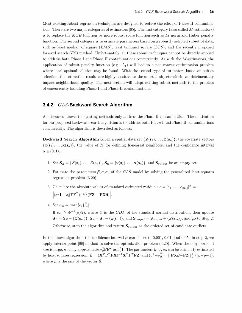
3.4.2 GLS-Backward Search Algorithm 36
Most existing robust regression techniques are designed to reduce the effect of Phase II contamina-
tion. There are two major categories of estimators [65]. The first category (also called M -estimators)
is to replace the MSE function by more robust score function such as L1 norm and Huber penalty
function. The second category is to estimate parameters based on a robustly selected subset of data,
such as least median of square (LMS), least trimmed square (LTS), and the recently proposed
forward search (FS) method. Unfortunately, all these robust techniques cannot be directly applied
to address both Phase I and Phase II contaminations concurrently. As with the M -estimators, the
application of robust penalty function (e.g., L1) will lead to a non-convex optimization problem
where local optimal solution may be found. With the second type of estimators based on subset
selection, the estimation results are highly sensitive to the selected objects which can detrimentally
impact neighborhood quality. The next section will adapt existing robust methods to the problem
of concurrently handling Phase I and Phase II contaminations.
3.4.2 GLS-Backward Search Algorithm
As discussed above, the existing methods only address the Phase II contamination. The motivation
for our proposed backward search algorithm is to address both Phase I and Phase II contaminations
concurrently. The algorithm is described as follows:
Backward Search Algorithm Given a spatial data set Z(s1), . . . , Z(sn), the covariate vectors
x(s1), . . . ,x(sn), the value of K for defining K-nearest neighbors, and the confidence interval
α ∈ (0, 1),
1. Set SZ = Z(s1), . . . , Z(sn), Sx = x(s1), . . . ,x(sn), and Soutput be an empty set.
2. Estimate the parameters βββ, σ, σ0 of the GLS model by solving the generalized least squares
regression problem (3.20).
3. Calculate the absolute values of standard estimated residuals e = [e1, . . . , e|SZ|]T =∣
∣
∣(σ2I + σ20FFT )−1/2(FZ − FXβββ)
∣
∣
∣.
4. Set em = maxei|SZ|i=1 .
If em ≥ Φ−1(α/2), where Φ is the CDF of the standard normal distribution, then update
SZ = SZ − Z(sm), Sx = Sx − x(sm), and Soutput = Soutput + Z(sm), and go to Step 2.
Otherwise, stop the algorithm and return Soutput as the ordered set of candidate outliers.
In the above algorithm, the confidence interval α can be set to 0.001, 0.01, and 0.05. In step 2, we
apply interior point [66] method to solve the optimization problem (3.20). When the neighborhood
size is large, we may approximate σ20FFT as σ2
0I. The parameters βββ, σ, σ0 can be efficiently estimated
by least squares regression: βββ = (XT FTFX)−1XTFT FZ, and (σ2+σ20) =‖ FXβββ−FZ ‖2
2 /(n−p−1),
where p is the size of the vector βββ.

3.4.3 GLS-Forward Search Algorithm 37
This backward search algorithm is designed based on the observation that top ranked outliers iden-
tified by the regular least squares method are still true outliers (in most cases) under both Phase I
and II contaminations. Suppose a true outlier s is removed after the first iteration, then both Phase
I and Phase II contaminations in the next iteration will be reduced. To illustrate this process, we
use the same example in Section 3.4. Recall that an outlier object Z∗(s) is decomposed into two
additive components Z∗(s) = Z(s)+ ζ, where Z(s) represents the normal value and ζ represents the
contamination error. Suppose s is the only outlier neighbor of an object s1 that happens to be an
outlier. Then the local difference diff(Z∗(s1)) = [Z(s1) −1K
∑
si∈N(s)(Z(si))] + ζ1 − ζ/K will be
marked as normal if ζ = K · ζ1. Suppose now that the true outlier Z(s) is removed and the newly
replaced neighbor for s1 is normal, then diff(Z∗(s1)) = [Z(s1) −1K
∑
si∈N(s)(Z(si))] + ζ1. This
local difference becomes an abnormal value and the masking effect is removed. Similarly, suppose
Z∗(s1) is a normal object, then its local difference is contaminated (swamped) by the error −ζ/K,
because of its outlier neighbor Z(s). The removal of s will make −ζ/K = 0 and therefore reducing
the swamping effect. For Phase II contamination, the removal of Z(s) leads to the removal of an
abnormal difference diff (Z∗(s)). The set of remaining local differences will therefore have less con-
tamination. The center of the distribution is less attracted by outliers, and the distributional shape
becomes less distorted. As a result, outliers tend to be more separated and normal objects tend to
be closer together. The masking and swamping effects are therefore reduced.
3.4.3 GLS-Forward Search Algorithm
This section adapts the popular Forward Search (FR) algorithm [65] to the GLS parameters esti-
mation problem. There are several restrictions to apply FR here. As discussed in Section 3.4.1, FR
starts from a robustly select subset of sample, but GLS is a statistical model based on neighborhood
aggregations. Considering only a subset of the observations Z(s1), . . . , Z(sn) will significantly im-
pact the quality of the calculated local differences. To apply FR algorithm, we make the assumption
that Phase I contamination is negligible compared to Phase II contamination. As discussed in Sec-
tion 3.4.1, this is reasonable for the case of isolated outliers. Based on this assumption, we consider
the local differences diff(Z(s1)), . . . , diff(Z(sn)) as pseudo “observations”, and then apply FR
algorithm to estimate the model parameters. By simulations, we also noticed that in this case
there is no significant difference between applying generalized least squares regression and regular
least squares regression. For the sake of efficiency, we only apply regular least squares regression to
estimate the parameters βββ, σ, and σ0. The FR algorithm is described as follows:
Forward Search algorithm Given a spatial data set Z(s1), . . . , Z(sn), the covariate vectors
x(s1), . . . ,x(sn), and the value of K for defining K-nearest neighbors,
1. Calculate the local differences: diff(Z) = FZ, and set Soutput be an empty set.
2. Set S = s1, . . . , sn; Set Z∗(S) = [Z∗(s1), . . . , Z∗(sn)] = diff(Z), and X∗(S) = [x∗(s1), . . . ,x
∗(sn)] =
FX, as the vector of pseudo “observations” and pseudo “covariates”.

3.4.4 Connections with Existing Methods 38
3. Apply least trimmed squares (LTS) [65] to find a robust subset of S, defined as S∗, and set
S∗test = S − S∗. The size of the subset S∗ is ⌊(n+ p+ 1)/2⌋ by default.
4. Estimate the parameter βββ based on Z∗(S∗) and X∗(S∗). Then calculate the absolute standard
residuals of S∗test as e =
√n−p−1|Z∗(S∗
test)−X∗(S∗
test)βββ|‖Z∗(S)−X∗(S)βββ‖2
.
5. Find the minimal residual of the test set S∗test:
em = mineiei∈S∗test
.
6. Update Soutput = Soutput + sm,S∗ = S∗ + sm,S∗test = S∗
test − sm. If S∗test is not empty,
go to step 4; otherwise, output the ordered set Soutput and terminate the algorithm.
The proposed FR algorithm provides an ordering of objects based on their agreements with the
GLS model. To identify outliers, it plots and monitors the change of the minimal residual with
the increasing size of the normal set S∗. A drastic drop implies that an outlier was added to
S∗. This plot could also help identify masked or swamped objects. Readers are referred to [65]
for details. A direct method for calculating the local differences can be achieved via robust mean
functions such as median and trimmed mean. However, as indicated by our simulation study, this
direct approach will deteriorate the performance of GLS. Recall that the statistical model of GLS:
diff(Z) ∼ N (FXβββ,FΣFT + σ20FFT ) . If we replace the left hand side diff(Z) = FZ by medians or
trimmed means, the right side will remain unchanged and thus still employs the average matrix F.
The increased bias caused by this inconsistency is much larger than the reduction of contamination
effects achieved through robust means.
3.4.4 Connections with Existing Methods
This section studies the connections between global (kriging) based [63–65], local spatial statistics
(LS) based methods [56–58,60,61,286,62], and the proposed GLS based SOD approach. First, we
review the first two approaches: Kriging-SOD and LS-SOD. The basic idea of Kriging-SOD is
to first apply robust methods to estimate the parameters of a global kriging model. The method
uses the estimated statistical model to predict the Z attribute of each sample location s, denoted as
Z(s), based on the Z values of other locations. The standardized residual (|Z(s)−Z(s)|/σs) follows
a standard normal distribution, where σs is the estimated standard deviation. If a residual is outside
the range [−Φ−1(α/2),Φ−1(α/2)], the corresponding object is reported as an outlier, where Φ is the
CDF and α is usually set 0.05. The LS-SOD approach assumes that diff(Z) ∼ N (1, σ2I). The
set of components in diff(Z) can be regarded as an i.i.d. sample of a univariate normal distribution
N (µ, σ). Robust techniques are designed to estimate µ and σ. The remaining steps are similar to
Kriging-SOD.
Theorem 5 Suppose that FΣFT = σ2I and the parameters of Kriging-SOD and GLS-SOD are
correctly calculated by robust estimation, then Kriging-SOD and GLS-SOD are equivalent.

3.4.4 Connections with Existing Methods 39
Proof
For Kriging-SOD, we consider a universal kriging model [53], since other kriging models (e.g.,
ordinary kriging) are its special cases. It suffices to prove that the standardized residuals cal-
culated by Kriging-SOD and GLS-SOD are identical. Without loss of generality, we test the
standardized residual of one particular sample point Z(sn). Let Z∗ = [Z(s1), . . . , Z(sn−1)]T and
Z = [Z∗T
, Z(sn)]T . By Section 3.3.1 Equation 3.3, Z ∼ N (Xβββ,D), where D = Σ+σ20I =
[
Σ∗ σσσ
σσσT σ2n
]
,
V ar(Z∗) = Σ∗, Cov(Z(s1),Z∗) = σσσ, and V ar(Z(sn)) = σ2
n.
Then, the standard residual by Kriging-SOD is
StdRsdKriging−SOD (Z(sn)) =[xT
nβββ + σσσT Σ∗−1
(Z∗ − X∗βββ)]
σn − σσσT Σ∗−1σσσ(3.22)
The standard residual by LS-SOD is
StdRsdKriging−SOD (Z(sn)) = StdRsdGLS−SOD (Z(sn)) (3.23)
The condition FΣFT = σ2I implies that σ2I + σ20FFT = FΣFT + σ2
0FFT = FDFT . Then, (σI +
σ0FFT )−1/2 = (FDFT )−1/2 = (FD1/2)−1 = D−1/2F−1. It follows that (σI + σ0FFT )−1/2(FZ −
FXβββ) = D−1/2F−1(FZ − FXβββ) = D−1/2(Z − Xβββ).
Further, given that D =
[
Σ∗ σσσ
σσσT σn
]
, it can be readily shown that
D−1/2 =
[
C−11 + C
−1/22 Σ∗−1
ββββββTΣ∗−1]1/2
0
−σσσTΣ∗−1
C−1/22 C
−1/22
, (3.24)
where C1 = Σ∗−1
− σnσσσσσσT and C2 = σn − σσσT ∗−1
σσσ.
Then, [(σI+σ0FFT )−1/2(FZ−FXβββ)]n = [D−1/2(Z−Xβββ)]n =
[
D−1/2
[
X∗βββ
xTnβββ
]
]
]
n
= −C−1/22 βββTΣ∗−1
X∗βββ+
C−1/22 xT
nβββ = xTnβββ + σσσT Σ∗−1
(Z∗ − X∗βββ)/(σn − σσσT Σ∗−1)
σσσ).
The above indicates that
StdRsdKriging−SOD (Z(sn)) = StdRsdGLS−SOD (Z(sn)) , (3.25)
We conclude that Kriging-SOD and GLS-SOD are equivalent.
Theorem 6 If FΣFT = σ2I, σ20FFT = σ2
0I, the parameters of GLS-SOD and LS-SOD are
correctly calculated by robust estimation, and one of the following conditions is true, then GLS-
SOD becomes equivalent to LS-SOD.
3.5 Simulations 40
1. Z(s) has a constant trend (mean): Xβββ = cI, where c is a constant value.
2. Z(s) is a linear trend of spatial coordinates, and each point s is the geometric center (or
centroid) of its neighbors.
Proof For either condition (1) or (2), it can be readily derived that FXβββ = 0. By conditions
FΣFT = σ2I and σ20FFT = σ2
0I, we have FZ ∼ N (0, (σ2 + σ20)I) which is consistent with the i.i.d.
assumption in LS-SOD. If we use the same robust methods to estimate the parameters, such as
using median and median absolute deviation (MAD) to estimate the mean and standard deviation
σ, then GLS-SOD becomes equivalent to LS-SOD.
Discussion: By Theorem 6, LS-SOD is a special form ofGLS-SOD. LS-SOD assumes V ar(diff(Z)) =
σ2I for some constant σ, but no justifications are presented. From this perspective, GLS-SOD ac-
tually provides a theoretical foundation for LS-SOD. Section 3.3.1 discusses the situations where
V ar(diff(Z)) can be approximated by (σ2 + σ20)I. Furthermore, under the conditions of Theorem
6, LS-SOD is equivalent to GLS-SOD and since the conditions also include “FΣFT = σ2I”, then
by Theorem 4 we have that GLS-SOD is equivalent to Kriging-SOD. Therefore, LS-SOD be-
comes equivalent to Kriging-SOD in this situation. Hence, it can be seen that the proposed GLS
framework can be parameterized to become instances of LS-SOD or Kriging-SOD. Further study
on various outlier detection methods can be greatly enhanced under the lens of this unifying GLS
framework.
As discussed in Section 3.3.1, FΣFT can be reasonably approximated by σ2I. From Theorem 5, the
major difference between Kriging-SOD and GLS-SOD is for which approach the related model
parameters can be estimated more accurately and efficiently. From this perspective, GLS-SOD is
superior to Kriging-SOD based on three major reasons: First, GLS-SOD has less uncertainty than
Kriging-SOD, since Kriging-SOD needs to further assume a semivariogram model. If the semi-
variogram model is not selected properly, the performance may be significantly impacted. Second,
GLS-SOD is a convex optimization problem and therefore a global optimal solution exists. How-
ever, Kriging-SOD is a non-convex optimization problem and relies on an iteratively reweighted
generalized least square (IRWGLS) approach [64] to determine a local solution. Finally, as shown
in Section 3.5 simulations, GLS-SOD runtime performance is superior to Kriging-SOD.
3.5 Simulations
This section conducts extensive simulations to compare the performance between the proposed
GLS based SOD methods and other related SOD methods. The experimental study follows the
standard statistical approach for evaluating the performance of spatial outlier detection methods
found in [63, 64, 53, 54].

3.5.1 Simulation Settings 41
3.5.1 Simulation Settings
Data set: The simulation data are generated based on the following statistical model:
Z(s) = xT (s)βββ + ω(s) + e(s) (3.26)
where ω(s) is a Gaussian random field with covariogram model C(h;θθθ).
We consider two popular covariogram models: spherical model and exponential model. See Equation
3.16 in Section 3.3.2 for the definition of a spherical model. The exponential model is defined as
C(h;θθθ = [b, c]T ) =
b, if h = 0, (3.27)
b(1 − exp(−h/c)), if 0 < h ≤ c, (3.28)
0, if h > c, (3.29)
These two models have the same parameters b and c. Recall that b is also the constant variance for
each Z(s).
For the trend component xT (s)βββ, we define x(s) = [1, x(s), y(s), x(s) ·y(s), x(s)2, y(s)2]T , where x(s)
and y(s) be the X and Y coordinates of the location s. This implies that the trend x(s)βββ is a
polynomial of order two. The nonlinearity of the trend is decided on the regression parameters βββ.
For example, if βββ = [1, 0, 0, 0, 0, 0]T ,then the trend is constant; if βββ = [1, 1, 1, 0, 0, 0]T , then the trend
is linear trend.
For the white noise component, we employ the following standard model [53]:
e(s) ∼
N (0, σ20), with probability 1 − α, (3.30)
N (0, σ2C), with probability α. (3.31)
There are three related parameters σ0, σC , and α. σ20 is the variance of a normal white noise, σ2
C is
the variance of contaminated error that generates outliers, and α is used to control the number of
outliers. Note that it is possible that the distribution N (0, σ2C) will also generate some normal white
noises. All true outliers must be only identified based on standard statistical test by calculating
the conditional mean and standard deviation for each observation [54]. We also consider the case
of clustered outliers. This can be simulated by constraining that the noises of a random cluster of
n · α points follow N (0, σ2C). In the simulations, we tested several representative settings for each
parameter, which are summarized in Table 3.2.
Outlier detection methods: We compared our methods with the state of the art local and global
based SOD methods, including Z-test [56], Median Z-test [58], IterativeZ-test [57], trimmedZ-
test [60], SLOM -test [61], and universal kriging (UK) based forward search [11,12] (noted as UK-
forward). Our proposed methods are identified as GLS-backward-G, GLS-backward-R, and GLS-
forward-R. GLS-backward-G refers to the GLS backward algorithm using generalized least squares
regression. GLS-backward-R refers to the GLS backward algorithm using regular least square
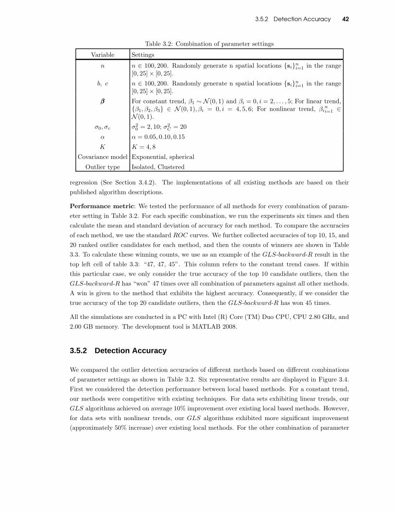
3.5.2 Detection Accuracy 42
Table 3.2: Combination of parameter settings
Variable Settings
n n ∈ 100, 200. Randomly generate n spatial locations sini=1 in the range
[0, 25]× [0, 25].
b, c n ∈ 100, 200. Randomly generate n spatial locations sini=1 in the range
[0, 25]× [0, 25].
βββ For constant trend, β1 ∼ N (0, 1) and βi = 0, i = 2, . . . , 5; For linear trend,β1, β2, β3 ∈ N (0, 1), βi = 0, i = 4, 5, 6; For nonlinear trend, βi
ni=1 ∈
N (0, 1).
σ0, σc σ20 = 2, 10; σ2
C = 20
α α = 0.05, 0.10, 0.15
K K = 4, 8
Covariance model Exponential, spherical
Outlier type Isolated, Clustered
regression (See Section 3.4.2). The implementations of all existing methods are based on their
published algorithm descriptions.
Performance metric: We tested the performance of all methods for every combination of param-
eter setting in Table 3.2. For each specific combination, we run the experiments six times and then
calculate the mean and standard deviation of accuracy for each method. To compare the accuracies
of each method, we use the standard ROC curves. We further collected accuracies of top 10, 15, and
20 ranked outlier candidates for each method, and then the counts of winners are shown in Table
3.3. To calculate these winning counts, we use as an example of the GLS-backward-R result in the
top left cell of table 3.3: “47, 47, 45”. This column refers to the constant trend cases. If within
this particular case, we only consider the true accuracy of the top 10 candidate outliers, then the
GLS-backward-R has “won” 47 times over all combination of parameters against all other methods.
A win is given to the method that exhibits the highest accuracy. Consequently, if we consider the
true accuracy of the top 20 candidate outliers, then the GLS-backward-R has won 45 times.
All the simulations are conducted in a PC with Intel (R) Core (TM) Duo CPU, CPU 2.80 GHz, and
2.00 GB memory. The development tool is MATLAB 2008.
3.5.2 Detection Accuracy
We compared the outlier detection accuracies of different methods based on different combinations
of parameter settings as shown in Table 3.2. Six representative results are displayed in Figure 3.4.
First we considered the detection performance between local based methods. For a constant trend,
our methods were competitive with existing techniques. For data sets exhibiting linear trends, our
GLS algorithms achieved on average 10% improvement over existing local based methods. However,
for data sets with nonlinear trends, our GLS algorithms exhibited more significant improvement
(approximately 50% increase) over existing local methods. For the other combination of parameter

3.5.3 Computational Cost 43
settings in Table 3.2, the winning statistics for each method are displayed in Table 3.3. These results
further justify the preceding performance results.
We also compared our GLS algorithms against the global based method UK-forward. Overall, our
methods were comparable to UK-forward. Particularly, GLS-backward-G attained better accuracy
than UK-forward on about half of the data sets. For the remaining data sets, the GLS-backward-G
is still competitive to the UK-forward. Additionally, as shown in Section 3.5.3, the UK-forward
incurs a significantly much higher computational cost than the GLS algorithms.
As discussed in Section 3.4.3, when K is small, the effects of σ20FFT must be considered and a gen-
eralized least regression is necessary. The theorems indicate that GLS-backward-G should perform
better then GLS-backward-R, this was justified in Figure 3.4 c).
Table 3.3: Competition statistics for different combinations of parameter settings
Algorithm Constant Trend Linear Trend Nonlinear Trend
GLS-backward-R 47, 47, 45 79, 72, 82 76, 81, 77
GLS-backward-G 88, 86, 89 114, 102, 120 141,144, 138
GLS-forward-R 13, 11, 14 22, 25, 27 40, 36, 47
Z-test 47, 35, 40 29, 30, 13 0, 0, 0
IterativeZ-test 35, 46, 63 16, 20, 21 0, 0, 0
MedianZ-test 20, 23, 29 1, 7, 8 0, 0, 0
TrimmedZ-test 15, 23, 32 5, 13, 13 0, 0, 0
SLOM -test 0,0, 0 0, 0, 0 0, 0, 0
Note: Each cell contains three values, representing the win timesfor the related method on the accuracies of top 10, 15, and 20ranked outlier candidates for all methods.
3.5.3 Computational Cost
The comparison on computational cost is shown in Figure 3.3. The results indicate that the time
cost of UK-forward is much higher than other methods. Even the second slowest method GLS-
backward-G, is still three times faster than UK-forward. The other local methods are approxi-
mately equal and hence much faster than UK-forward.
From the comparisons of both the accuracy and computational cost, it can be seen that our proposed
GLS-SOD algorithms (especially GLS−backward−G) is significantly more accurate than existing
local based algorithms when the spatial data exhibits either a linear or nonlinear spatial trend.
Our GLS algorithms are comparable to the global based method UK-forward on accuracy, but
significantly faster than UK-forward.

3.5.4 Conclusion 44
Figure 3.3: Comparison on computational cost (setting: linear trend, isolated outliers,α = 0.1, σ2
0 = 2, c = 15,K = 8, n = 200)
3.5.4 Conclusion
This chapter presents a generalized local statistical (GLS) framework for existing local based meth-
ods. This generalized statistical framework not only provides theoretical foundations for local based
methods, but can also significantly enhance spatial outlier detection methods. This is the first work
to present the theoretical connection between local and global based SOD methods under the GLS
framework.

3.5.4 Conclusion 45
(a) Constant trend, isolated outliers,α = 0.1, σ2
0 = 2, c = 15, K = 4(b) Linear trend, isolated outliers,
α = 0.1, σ20 = 2, c = 15, K = 8
(c) Nonlinear trend, isolated outliers,α = 0.15, σ2
0 = 10, c = 15, K = 4(d) Constant trend, clustered outliers,
α = 0.1, σ20 = 2, c = 25, K = 4
(e) Linear trend, clustered outliers,α = 0.15, σ2
0 = 2, c = 25, K = 8(f) Nonlinear trend, clustered outliers,
α = 0.15, σ20 = 10, c = 5, K = 8
Figure 3.4: Outlier ROC Curve Comparison (the same setting: n = 200, b = 5, σ2C = 20)

Chapter 4 46
Chapter 4
A GeneralizedApproach toNon-Numerical SpatialOutlier Detection
4.1 Introduction
Spatial outlier (anomaly) detection is an important problem that has received much attention in
recent years. Most existing methods are focused on numerical data, but in real world applications
we are often faced with a variety of data types. For example, in the field of disease surveillance, we
are monitoring public health data sources, such as medical sales (numerical attributes) and hospital
visits (count attributes). In the field of economics studies, the living areas (numerical attributes)
and the indicator which shows if a dwelling is located in a certain country (binary attributes) are
measured to characterize house sale prices. In the field of agriculture, the combinations (nominal
attributes) of soils are measured to study the geographic distribution of different plan types.
The traditional outlier detection algorithms can be classified into the following categories: clustering-
based, distribution-based, depth-based, density-based, and distance-based. Most of these approaches
are designed for numerical attributes, whereas real world datasets are usually of non-numerical data
types, such as binary, count, ordinal, and normal attributes. Direct application of these approaches
to non-numerical data leads to the loss of significant correlations between data objects, and their
extension to non-numerical data is also technically challenging. For example, the distance based
approach relies on well-defined measures to calculate the proximity between data observations, but
there is no unified distance measure that can be used for non-numerical attributes. The statistical
model based approach relies on the modeling of correlations between attributes, but there is no
4.1 Introduction 47
unified correlation measure available for non-numerical attributes.
There exists only one method designed for dealing with non-numerical spatial data, namely, pair
correlation function (PCF) based [303]. The authors propose a new metric, namely Pair Correlation
Ratio (PCR), to measure the spatial correlations between spatial categorical observations. The
PCR values are then applied to calculate the weights of neighbors to estimate the probability of a
given object being an outlier, and the weighted average of its neighbors is used as the estimator.
Note that, a number of methods have been proposed for general categorical datasets, which can be
grouped into four categories: rule based [1, 7, 15, 16, 26, 36], probability distribution based [6, 10,
25, 27], entropy based [13, 14], and similarity based [5, 28]. Because these general outlier methods
do not take spatial correlations in consideration, these general methods cannot be directly applied
to spatial categorical data.
To the best of our knowledge, there is no existing work that is able to address the following challenges
concurrently for spatial non-numerical outlier detection: 1) How to develop a unified framework
that can model spatial correlations for a variety of data types, such as binary, nominal, ordinal,
and count? 2) How to model large data variations caused by outliers? 3) How to develop an
efficient detection algorithm that is scalable for large spatial datasets? In this paper, we present a
statistical outlier detection model to address the preceding three challenges. We begin by presenting
a Bayesian generalized spatial linear model to model spatial correlations for a variety data types
characterized by the exponential distribution family. We then incorporate an additional “error
buffer” component based on Student-t distribution to capture the large variations caused by outliers.
Student-t distribution has been widely used in robust statistics to minimize the effects of outliers
in a variety of applications [10, 11]. After that, we integrate a latent reduced-rank spatial Kriging
model and present a approximate inference algorithm that can conduct the outlier detection process
in linear time.
The main contributions of our work can be summarized as follows:
• Design of a Robust and Reduced Rank Bayesian SGLMM (3RB-SGLMM) model.
A new 3RB-SGLMM model is developed, which integrates the advantages of SGLMM, robust
SLM, reduced-rank GLM, and Bayesian hierarchical model. Readers are referred to Chapter
2 about these four traditional models. This model supports all the data types characterized
by the family of exponential distribution. Although it still does not avoid the problem of high
dimensionality in the latent random variables, the special conditional independence structure
makes it possible to develop efficient detection algorithms with a linear time time complexity.
• Develop of an efficient algorithm for robust parameter estimation. The posterior
distribution of latent variables the 3RB-SGLMM model is approximated by Gaussian distri-
bution, and the model is calculated by iterative reweighted least squre (IRLS). The posterior
distribution of the model parameters are then estimated by Laplace approximation. Efficient
matrix manipulations are designed to guarantee that the whole estimate process can be done
in linear time.

4.2 Theoretical Preliminaries 48
• Design of an efficient algorithm for non-numerical spatial outlier detection. Given
the designed 3RB-SGLMM model, the outlier detection problem is then addressed by estimat-
ing the posterior distribution of the “error buffer” random variables that follow a Student-t
prior distribution. An efficient algorithm based on Gaussian and Laplace approximation tech-
niques to estimate the mode and Hessian of the negative log posterior, which are then used to
form an approximate Gaussian distribution for outlier detection.
• Comprehensive experiments to validate the effectiveness and efficiency of the pro-
posed techniques. We conducted extensive experiments on both simulation and real-life
datasets. The detection accuracy, time complexity, as well as the impact of parameters, are
evaluated, and the results demonstrated the good performance of our proposed non-numerical
spatial outlier detection approach.
The rest of the chapter is organized as follows. Section 4.2 presents theoretical preliminaries, in-
cluding reduced-rank spatial linear model and spatial generalized linear model (SGLM). Section 4.3
formulates a new robust and reduced rank Bayesian SGLM model, and discusses its connection with
traditional spatial models. Section 4.4 designs efficient algorithms to infer latent variables, estimate
model parameters, and detect non-numerical spatial outliers. Section 4.5 evaluates the effectiveness
and efficiency of our proposed techniqeus using both simulation and real life datasets. Section 4.6
concludes with a summary of our major work.
4.2 Theoretical Preliminaries
This section introduces two fundamental spatial statistical models, including Reduced-Rank Spatial
Linear Model (RR-SLM) and spatial generalized linear mixed Model (SGLMM).
4.2.1 Reduced-Rank Spatial Linear (Gaussian Process) Mode l
Spatial inferences (e.g., spatial prediction, outlier detection) based on the SLM model involve the
inversion of the N by N correlation matrix R(φ), which has the time complexity O(N3). This
characteristic makes the SLM model unscalable to large datasets. In order to increase the scalability,
Banerjee et al. proposed a reduced rank SLM model based on a set of knots s∗1, · · · , s∗M. The basic
idea is to estimate latent variables η(s1), · · · , η(sN based on η(s∗1), · · · , η(s∗M ) by using spatial
Kriging [45].
η = cT R∗(φ)−1η∗, (4.1)
η∗ ∼ N (0, σ2R∗(φ)), (4.2)

4.2.2 Spatial Generalized Linear Mixed Model (SGLMM) 49
where η∗ = [η(s∗1), · · · , η(s∗m)]T , R∗
ij(φ) = C(η(s∗i ), η(s∗j )|φ), and ci = C(η(s), η(s∗i )|φ). The reduced
rank SLM model can be formalized as
Y = Xβ + η + ε
η = cT R∗(φ)−1η∗,
η∗ ∼ N (0, σ2R∗(φ)),
ε ∼ N (0, τ2I). (4.3)
It is important to select a reasonable number of knots as well as their spatial locations. This is
related to the problem of spatial design and a rich literature can be found ( [46], [45]). There are
two popular knots selection strategies. This first one is to draw a uniform grid to cover the study
region and each grid point is regarded as a knot. The second one is to place knots such that each
knot covers a local domain and the regions that have dense data have more knots. In practice, it
is feasible to validate models by using different number of knots and different choices of knots to
obtain a reliable and robust configuration.
4.2.2 Spatial Generalized Linear Mixed Model (SGLMM)
The spatial generalized linear mixed model (SGLMM) can be described by a two-layer hierarchical
structure, including the observations and the latent Gaussian process layers.
• The Observations Layer
Let Y (s) be a response variable at locations s ∈ D ⊂ R2. It is assumed that Y (s) follows an
exponential family distribution with the probability density
f(Y (s)|θ(s), τ) = exp
(
Y (s)θ(s) − a(θ(s))
d(τ)+ h(Y (s), τ)
)
, (4.4)
where θ(s) and τ are model parameters. θ(s) is related to the mean of the distribution that
varies by location, and τ is called the dispersion parameter and is related to the variance of
the distribution. The functions h(y(s), τ), a(θ(s)), and d(τ) are known. Y (s) has mean and
variance
E(Y (s)) := µ(s) = a′(θ(s)), (4.5)
V ar(Y (s)) := σ(s)2 = a′′(θ(s))d(τ), (4.6)
where a′(θ(s)) and a′′(θ(s)) are the first and second derivatives of a(θ(s)). Many popular
distributions belong to this family, such as Gaussian, exponential, Binomial, Poisson, gamma,
and inverse Gaussian, Dirichlet, and chi-squared beta distributions.

4.3 Robust and Reduced-Rank Bayesian SGLMM model 50
• The Latent Spatial Gaussian Process Layer
Each random variable Y (s) in the observation layer is related to a latent random variable
(η(s)) through its mean (µ(s)) and a link function
g(µ(s)) = η(s) := x(s)Tβ + η(s), (4.7)
where x(s) refers to a vector of covariates and β refers to the vector of regression parameters.
The component η(s) follows a zero mean spatial Gaussian process as introduced in Section 2.1
η(s) ∼ GP(
0, σ2C(η(s), η(s′)|φ))
.
Given the observations Y = Y (s1), · · · , Y (sN ), a discretized form of the SGLMM model can be
described as
Y (sn) ∼ Exp(θ(sn), τ), n = 1, · · · , N,
µ = a′(θ),
g(µ) = Xβ + η,
η ∼ N (0, σ2R(φ)), (4.8)
where θ = [θ(s1), · · · , θ(sN )]T , a′(θ) = [a′(θ(s1)), · · · , a′(θ(sN ))]T , and Exp(θ(sn), τ) refers to an
exponential family distribution with the probability density
f(Y (sn)|θ(sn), τ) = exp
(
Y (sn)θ(sn) − a(θ(sn))
d(τ)+ h(Y (sn), τ)
)
. (4.9)
4.3 Robust and Reduced-Rank Bayesian SGLMM model
This section presents a Robust and Reduced-Rank Bayesian SGLMM model (3RB-SGLMM), which
integrates the advantages of SGLMM, robust SLM, reduced-rank GLM, and Bayesian hierarchical
model. The 3RB-SGLMM model can be formalized in the framework of Bayesian hierarchical model
with three layers, including the observations layer, the latent robust Gaussian process layer, and the
parameters layer. The graphic representation of the 3RB-SGLMM model is shown in Figure 4.1.
4.3.1 The Observations Layer
Given the observations Y = [Y (s1), · · · , Y (sN )], denote Yn = Y (sn). It is assumed that each Y (sn)
follows a distribution of exponential family
Yn ∼ Exp(θn, τ), n = 1, · · · , N,

4.3.1 The Observations Layer 51
Figure 4.1: Graphic Model Representation of the 3RB-SGLMM Model
where θn and τ refer to the distribution parameters, θn is related to the mean of the distribution
that varies by location sn, and τ is called the dispersion parameter and is related to the variance of
the distribution. The probability density function f(Yn|θn, τ) has the form
f(Yn|θn, τ) = exp
(
Ynθn − a(θn)
d(τ)+ h(Yn, τ)
)
, (4.10)
in which the specifications of functions θn, a(θn), d(τ), and h(Yn, τ) are defined based on the specific
distribution considered, such as poisson, binomial, and gamma distributions. For example, the
Binomial distribution B(mn, πn) has the density
p(Yn) =
(
mn
Yn
)
πYnn (1 − πn)mn−Yn . (4.11)
Taking logs, we can rewrite the density function as
log p(Yn) = Yn log(πn
1 − πn) +mn log(1 − πn) + log
(
mn
Yn
)
. (4.12)
This shows that θn = log( πn
1−πn), a(θn) = mn log(1 + exp θn), and h(Yn, τ) = log
(
mn
Yn
)
, where the
second term in the density function is rewritten as log(1 − πn) = − log(1 + exp θn).

4.3.2 The Latent Robust Gaussian process Layer 52
4.3.2 The Latent Robust Gaussian process Layer
The observations Yn are mapped to latent robust Gaussian process random variables µn through
the link function
g(a′(θn)) = µ, (4.13)
where the link function g(·) is defined on the specific distribution of Yn. For example, for binomial
and poisson distributions, the link functions are defined as g(x) = ln(x/(1 − x)) and g(x) = lnx,
respectively.
Denote µ = [µ1, µ2, · · · , µN ]. The vector of latent robust Gaussian process random variables µ has
the additive form
µ = Xβ + η + ξ,
ξn ∼ Student′t(0, ν, σξ), n = 1, · · · , N, (4.14)
where Xβ refers to the large-scale trend component, β refers to the vector of generalized regression
parameters, η refers to the micro-scale spatial Gaussian process component, and ξ refers to the
“error buffer” component that is added to absorb large variations caused by outliers. Each random
variable ξn follows a Student-t distribution that has a heavy tail in its portability density function.
The micro-scale spatial Gaussian process component η is characterized by a reduced rank spatial
linear model
η = CR∗(φ)−1η∗,
η∗ ∼ N (0, σ2R∗(φ)),
where η∗ = [η(s∗1), · · · , η(s∗m)]T , R∗
ij(φ) = C(η(s∗i ), η(s∗j )|φ), ci = C(η(s), η(s∗i )|φ), and C(·) refers
to a kernel function, such as exponential or Gaussian kernels. In this work, we used the popular
exponential kernel, but our model supports other kernels as well.
4.3.3 The Parameters Layer
The proposed 3RB-SGLMM model has the major parameters β, σ2, σ2ξ , φ, ν, and τ . We present a
Bayesian framework that makes it convenient to integrate prior or domain knowledge. The param-
eters are themselves treated as random variables, and the second-level parameters are known as

4.3.4 Theoretical Interpretation 53
hyper-parameters. The prior distributions are defined as
β ∼ N (µβ ,Σβ),
σ2 ∼ Inv −Gamma(ασ2 , γσ2),
σ2ξ ∼ Inv −Gamma(ασ2
ξ, γσ2
ξ),
φ ∼ Uniform(aφ, bφ),
ν ∼ Uniform(aν , bν),
τ ∼ (ατ , γτ ), (4.15)
where, for the equation “τ ∼ (ατ , γτ )”, we did not state the specific prior distribution of the
dispersion parameter τ , which is dependent on the specific exponential family distribution used
in the model (see Equation (4.10)). For example, for Gaussian distribution or inverse Gaussian
distribution, τ is assigned a inverse Gamma prior, i.e., τ ∼ IG(alphaτ , γτ ). For poisson distribution
or binomial distribution, τ is identical to 1, an non-stochastic value, and no prior distributions
are needed. For gamma distribution or exponential distribution, τ is assigned a gamma prior, i.e.,
τ ∼ Gamma(alphaτ , γτ ).
4.3.4 Theoretical Interpretation
Our proposed 3RB-SGLMM model can be regarded as a general framework for robust spatial in-
ferences. For example, if the original sampled locations s1, · · · , sN are selected as knots, then
the 3RB-SGLMM model de-generalizes to a robust Bayesian SGLMM model. If we further set all
prior distributions as uniform distributions, then the 3RB-SGLMM model de-generalizes to a robust
SGLMM model [256]. If the Gaussian distribution is further selected as the exponential family dis-
tribution, then the 3RB-SGLMM model de-generalizes to a robust GLM model (Equation (2.24)).
If we further set the degrees of freedom parameter to infinity, then the variational component ξn
follows a Gaussian distribution, and hence the 3RB-SGLMM model de-generalizes to a regular GLM
model (Equation (2.22)).
4.4 Robust Approximate Inference
This section presents efficient algorithms to estimate the posterior distributions of latent robust
Gaussian process variables η∗, ξ, model parameters β, φ, σ2, τ, ν. Based on the estimated pos-
teriors, we then present an efficient algorithm to detect non-numerical outliers. Lastly, we show that
all the preceding processes can be conducted in linear time.

4.4.1 Inference on Latent variables 54
4.4.1 Inference on Latent variables
For the purpose of computational convenience, we treat the vector of regression parameters β as
latent variables, instead of model parameters. Denote ω = [η∗,β, ξ]. The objective is to inference
the Gaussian approximation of the posterior p(ω|Y,Θ; Ω), where Θ = [τ, φ, ν, σ2ξ , σ
2] and Ω refers
to the set of hyper-parameters. Given the mode ω and Hessian Σ−1 of the negative log density
function log p(ω|Y,Θ; Ω), the posterior can then be approximated as
p(ω|Y,Θ; Ω) ≈ q(ω|Y,Θ; Ω) = N (ω,Σ). (4.16)
The mode ω can be calculated by solving the optimization problem ω = argminω
log p(ω|Y,Θ; Ω),
and the Hessian at the mode ω can be obtained by applying a second order Taylor expansion of
log p(ω|Y,Θ; Ω):
Σ−1 = −∇2 log p(ω|Y,Θ; Ω)∣
∣
ω=ω= HTGH + diag(R∗,Q), (4.17)
where H = [CT R∗−1,X, I]; R∗i,j = C(|s∗i − s∗j |;φ) for two knot locations s∗i and s∗j ; Ct,n = C(|sn −
st|;φ) for a knot location s∗t and an observation location sn; G is a diagonal matrix and Gn is the
Hessian of the negative log observation density function − log p(Yn|Xβ+ CTR∗−1η∗ + ξ); and Q is
a diagonal matrix with the form
Qnn =νσ2
ξn− ξ2n
ξ2n + νσ2ξn
(ν + 1). (4.18)
The specific form of Gn is decided based on the distribution of observations. For example, if the
observations follow a Binomial distribution , then Gn has the form
Gn = mnexp(xn)
(1 + exp(xn))2, (4.19)
where xn = [Xβ + CT R∗−1η∗ + ξ]n, and mn refers to the number of trials at location sn. If the
observations follow a Poisson distribution instead, then Gn has the form
Gn = exp(xn). (4.20)
The mode ω can be identified using general numerical optimization techniques, such as gradient
decent, Newton’s methods, and interior point methods. In our work, we employed the popular
iterative re-weighted least squares (IRLS) algorithm for generalized linear models that optimizes
the mode ω and Hessian Σ−1 jointly, and in practice a good approximation can be obtained in five
iterations for the task of non-numerical outlier detection.

4.4.2 Inference on Parameters 55
4.4.2 Inference on Parameters
This section presents an approximate algorithm based on Laplace approximation to infer the poste-
rior of model parameters p(ω|Y; Ω), by marginalizing out the latent variables Θ:
p(ω|Y; Ω) =
∫
p(ω,Θ|Y; Ω)dΘ. (4.21)
The above integration process is analytical intractable, and approximate inference techniques must
be applied. Because the posterior p(ω|Y; Ω) is skewed, Gaussian approximation is hence inappro-
priate. We first reformulate the posterior as the form
p(ω|Y; Ω) ∝p(Y|ω,Θ; Ω)p(ω|Θ; Ω)p(Θ; Ω)
p(ω|Y,Θ; Ω). (4.22)
As shown in Section 4.4.1, the denominator p(ω|Y,Θ; Ω) ≈ N (ω,Σ). Laplace approximation on
the right component of Equation 4.22 can be obtained as
p(Θ|Y; Ω) ≈ q(ω|Y; Ω) ∝p(Y|ω,Θ; Ω)p(ω|Θ; Ω)p(Θ; Ω)
p(ω|Y,Θ; Ω)
∣
∣
ω=ω. (4.23)
Because the posterior p(ω|Y,Θ; Ω) is skewed, the mode Θ and Hessian ΣΘ of the negative log
density function q(ω|Y; Ω) are not accurate to characterize the distribution. A more appropriate
strategy is to sample K contour points Θ1, · · · ,ΘK around the mode Θ, and then calculate the
corresponding posteriors q(Θ1|Y; Ω), · · · , q(ΘK |Y; Ω). After normalization, we obtain the weights
∆1, · · · ,∆k, in which∑
k ∆k = 1. The most challenging step is to calculate the mode Θ. First,
the mode can be obtained by solving the following optimization problem
argminΘ
− log p(Y|ω(Θ),Θ; Ω) − log p(ω(Θ)|Θ; Ω) − log p(Θ; Ω) + log q(ω(Θ)|Y,Θ; Ω), (4.24)
where ω(Θ) is the mode of p(ω|Y,Θ; Ω), which is a function of Θ. The Hessian of the negative log
density function − log q(ω(Θ)|Y,Θ; Ω) has been estimated in Section 4.4.1, and those of the other
components can be readily derived. In addition, the above problem is a low dimensionality problem,
since there are only five variables in Θ. It can be efficiently solved by using numerical optimization
techniques, such as scaled conjugate gradients and Newton’s methods.
4.4.3 Non-Numerical Spatial Outlier Detection
As shown in the proposed 3RB-SGLMM model, the “error buffer” variables ξ1, · · · , ξN are designed
to absorb large variations caused by outliers. The anomaly degree of an observation Yn will be
characterized by the anomaly degree of the corresponding variable ξn. The posterior p(ξ|Y,Θ; Ω)

4.4.3 Non-Numerical Spatial Outlier Detection 56
can be calculated as
p(ξ|Y,Θ; Ω) =
∫
p(ξ,β,η∗|Y; Ω)dβdη∗
=
∫
p(ξ,β,η∗|Y,Θ; Ω)p(Θ|Y; Ω)dΘdβdη∗
≈
∫
q(ξ,β,η∗|Y,Θ; Ω)p(Θ|Y; Ω)dΘdβdη∗
≈K∑
k=1
∆k
∫
q(ξ,β,η∗|Y,Θk; Ω)dβdη∗
=
K∑
k=1
∆kq(ξ|Y,Θk; Ω)
= N
(
ωξ,
K∑
k=1
∆2kΣξ
)
, (4.25)
where q(ξ,β,η∗|Y,Θ; Ω) = N (ω,Σ) has been obtained in Section 4.4.1, and the contour sample
points Θ1, · · · ,ΘK have been obtained in Section 4.4.2, and q(ξ|Y,Θk; Ω) = N (ωξ,Σξ) is a
subspace distribution of q(ξ,β,η∗|Y,Θ; Ω). Based on the preceding result, the 3RB-SGLMM model
based non-numerical spatial outlier detection algorithm can be described as follows:
1. Estimate the approximate posterior p(ω|Y,Θ; Ω) ≈ N (ω,Σ) by Equations 4.16 and 4.17.
2. Estimate the contour sample points of model parameters Θ1, · · · ,ΘK and the corresponding
weights ∆1, · · · ,∆K by Equations 4.23 and 4.24.
3. Estimate the approximate posterior q(ξ|Y,Θ; Ω) = N(
ωξ,∑K
k=1 ∆2kΣξ
)
by Equation 4.25.
4. Calculate the normalized Gaussian distribution q(ξ|Y,Θ; Ω) = N (0, I), where
ξ = (K∑
k=1
∆2kΣξ)
1/2(ξ − β). (4.26)
5. The absolute value ξn is returned as an estimate of the anomaly degree of the objection Yn and
the set Soutliers of candidate outliers can be calculated using the standard Z test statistics:
Soutliers = Yn||ξ| > 3. (4.27)
At step 5, the square root of the matrix (∑K
k=1 ∆2kΣξ)
1/2 has the time cost O(N3), which is in-
appropriate for large datasets. In our implementation, we further approximate the matrix Σξ as a
diagonal matrix, which makes the time cost down to O(N).

4.4.4 Time and Space Complexity Analysis 57
4.4.4 Time and Space Complexity Analysis
This section analyzes the space and time costs of the above three inferences discussed in Sections
4.4.1 to 4.4.3. First, for the inference of latent variables, we applied the popular IRLS algorithm to
estimate the mode ω and Hessian Σ−1 jointly. Suppose the required number of iterations is L. For
each iteration the dominated time cost is the inversion of the matrix [HTGH+ diag(R∗,Σβ,Q)] as
shown in Equation 4.17, where H = [CT R∗−1,X, I], R∗ ∈ RM×M , C ∈ RM×N , X ∈ RN×P , and
I ∈ RN×N , G ∈ RN×N , Q ∈ RN×N . The counts N,M, and P refer to the numbers of observations,
knots, and regression attributes (predictors), respectively. Without any matrix optimization, the
time cost of the inversion is O(N3).
However, the special structure of the matrix can be explored and the time cost of the inversion can
be reduced to O(N(M + P )3). Specifically, denote F = CTR∗−1,X and A = GF, F∗ = FT GF.
Then the component HTGH has the decomposition form
(
F∗ AT
A G
)
.
The matrix HTGH + diag(R∗,Σβ,Q) then has the decomposition form
(
F∗ + diag(R∗,Σβ) AT
A G + Q
)
.
According to matrix algebra, the inverse of the above form has the special structure
(
C−1 C12
CT12 C−1
2
)
,
where
C1 = F∗ + diag(R∗,Σβ) − AT (G + Q)−1A,
C2 = G + Q− A(F∗ + diag(R∗,Σβ))−1AT ,
C12 = −(F∗ + diag(R∗,Σβ))−1AT (G + Q)−1.
By the ShermanCMorrisonCWoodbury formulae, the inversion C−12 have the decomposition
C−12 = (G + Q)−1 − (G + Q)−1A
(
F∗ + diag(R∗,Σβ) + AT (G + Q)−1A)−1
A(G + Q)−1.
Based on the above matrix manipulation, the inversion of the matrix [HTGH + diag(R∗,Σβ,Q)]
can be calculated in the time cost N(M + P )3. Note that, the inversions of the matrices Q and R
have linear time cost O(N), since they are both diagonal matrices. Therefore, the total time cost of
the inference of the latent variables ω is O(LN(M + P )3).

4.5 Experiments 58
Second, for the inference of parameters, we applied Laplace approximation to estimate the posterior
of the vector of parameters Θ. The main time cost lies on the calculation of the mode Θ, in which we
applied Trust Region Reflective algorithm, the default setting of the fmincon function in Matlab
R2011b. Suppose the required number of iterations is W . For each iteration, the main cost lies
on the inference of latent variables based on the current estimated Θ value and on the inversion
of the variance-covariance matrix of knots, which has the time cost O(LN(M + P )3) + O(M3) =
O(LN(M + P )3). Therefore, the total time cost of this inference process is O(MLN(M + P )3)
Third, for the non-numerical outlier detection process, Step 1 has the time cost O(LN(M + P )3),
Step 2 has the time cost O(MLN(M +P )3). Steps 3 to 5 have the time cost O(KN). The total cost
of the outlier detection process is O(MLN(M + P )3). The required number (L) of IRLS iterations
is smaller than 5 in practice, and the required number of iterations for inferring the mode Θ is
the same scale as the size of Θ that equals 5. In addition, the number (M) of knots and that of
regression parameters are both negligible when the data set size N is large. To conclude, for large
data sets, we have the linear time cost O(N) for all the three inferences. It can be readily derived
that the total space cost is O(N) as well.
4.5 Experiments
This section evaluates the effectiveness and efficiency of our proposed techniques using both four
simulation and six real life datasets. We focused on binary datasets as a case study, but our proposed
techniques can also be applied to all data types that can be characterized by the family of exponential
distribution, such as count, ordinal, and nominal attributes. All the experiments were conducted
on a PC with Intel(R) Core(TM) I7-Q740, CPU 1.73Ghz, and 8.00 GB memory. The development
tool was MATLAB 2011. Note that, we re-implemented all the competitive methods based on their
original papers in our experiments, because the original implementations are unavailable. Although
we have strictly followed the rules of these papers, it is not guaranteed that we have fully accurately
implemented those methods and optimally tuned the related parameters.
it is still potentially possible that our implementations have some inappropriate components.
4.5.1 Experiment Settings
Simulation Datasets
The simulation datasets were generated based on the regular spatial generalized linear Mixed model
(SGLMM)
Y (s) ∼ Binomial(m, g(µ(s))),
g(µ(s)) = x(s)Tβ + η(s),
η(s) ∼ GP(0, σ2C(|s − t|);φ), (4.28)
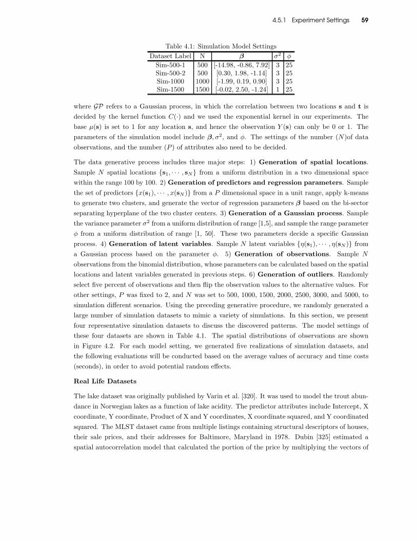
4.5.1 Experiment Settings 59
Table 4.1: Simulation Model Settings
Dataset Label N β σ2 φ
Sim-500-1 500 [-14.98, -0.86, 7.92] 3 25Sim-500-2 500 [0.30, 1.98, -1.14] 3 25Sim-1000 1000 [-1.99, 0.19, 0.90] 3 25Sim-1500 1500 [-0.02, 2.50, -1.24] 1 25
where GP refers to a Gaussian process, in which the correlation between two locations s and t is
decided by the kernel function C(·) and we used the exponential kernel in our experiments. The
base µ(s) is set to 1 for any location s, and hence the observation Y (s) can only be 0 or 1. The
parameters of the simulation model include β, σ2, and φ. The settings of the number (N)of data
observations, and the number (P ) of attributes also need to be decided.
The data generative process includes three major steps: 1) Generation of spatial locations.
Sample N spatial locations s1, · · · , sN from a uniform distribution in a two dimensional space
within the range 100 by 100. 2) Generation of predictors and regression parameters. Sample
the set of predictors x(s1), · · · , x(sN ) from a P dimensional space in a unit range, apply k-means
to generate two clusters, and generate the vector of regression parameters β based on the bi-sector
separating hyperplane of the two cluster centers. 3) Generation of a Gaussian process. Sample
the variance parameter σ2 from a uniform distribution of range [1,5], and sample the range parameter
φ from a uniform distribution of range [1, 50]. These two parameters decide a specific Gaussian
process. 4) Generation of latent variables. Sample N latent variables η(s1), · · · , η(sN ) from
a Gaussian process based on the parameter φ. 5) Generation of observations. Sample N
observations from the binomial distribution, whose parameters can be calculated based on the spatial
locations and latent variables generated in previous steps. 6) Generation of outliers. Randomly
select five percent of observations and then flip the observation values to the alternative values. For
other settings, P was fixed to 2, and N was set to 500, 1000, 1500, 2000, 2500, 3000, and 5000, to
simulation different scenarios. Using the preceding generative procedure, we randomly generated a
large number of simulation datasets to mimic a variety of simulations. In this section, we present
four representative simulation datasets to discuss the discovered patterns. The model settings of
these four datasets are shown in Table 4.1. The spatial distributions of observations are shown
in Figure 4.2. For each model setting, we generated five realizations of simulation datasets, and
the following evaluations will be conducted based on the average values of accuracy and time costs
(seconds), in order to avoid potential random effects.
Real Life Datasets
The lake dataset was originally published by Varin et al. [320]. It was used to model the trout abun-
dance in Norwegian lakes as a function of lake acidity. The predictor attributes include Intercept, X
coordinate, Y coordinate, Product of X and Y coordinates, X coordinate squared, and Y coordinated
squared. The MLST dataset came from multiple listings containing structural descriptors of houses,
their sale prices, and their addresses for Baltimore, Maryland in 1978. Dubin [325] estimated a
spatial autocorrelation model that calculated the portion of the price by multiplying the vectors of

4.5.1 Experiment Settings 60
10 20 30 40 50 60 70 80 90 100
10
20
30
40
50
60
70
80
90
100 0
0.1
0.2
0.3
0.4
0.5
0.6
0.7
0.8
0.9
1
(a) Sim-500-1
10 20 30 40 50 60 70 80 90 100
10
20
30
40
50
60
70
80
90
100 0
0.1
0.2
0.3
0.4
0.5
0.6
0.7
0.8
0.9
1
(b) Sim-1000
10 20 30 40 50 60 70 80 90 100
10
20
30
40
50
60
70
80
90
100 0
0.1
0.2
0.3
0.4
0.5
0.6
0.7
0.8
0.9
1
(c) Sim-1500
10 20 30 40 50 60 70 80 90 100
10
20
30
40
50
60
70
80
90
100 0
0.1
0.2
0.3
0.4
0.5
0.6
0.7
0.8
0.9
1
(d) Sim-500-2
Figure 4.2: Spatial Distribution of Four Simulation Datasets

4.5.1 Experiment Settings 61
10 20 30 40 50 60 70 80 90 100
10
20
30
40
50
60
70
80
90
100 0
0.1
0.2
0.3
0.4
0.5
0.6
0.7
0.8
0.9
1
(a) MLST
10 20 30 40 50 60 70 80 90 100
10
20
30
40
50
60
70
80
90
100 0
0.1
0.2
0.3
0.4
0.5
0.6
0.7
0.8
0.9
1
(b) LoaLoa
10 20 30 40 50 60 70 80 90 100
10
20
30
40
50
60
70
80
90
100 0
0.1
0.2
0.3
0.4
0.5
0.6
0.7
0.8
0.9
1
(c) BEF
10 20 30 40 50 60 70 80 90 100
10
20
30
40
50
60
70
80
90
100 0
0.1
0.2
0.3
0.4
0.5
0.6
0.7
0.8
0.9
1
(d) BostonSMSA
10 20 30 40 50 60 70 80 90 100
10
20
30
40
50
60
70
80
90
100 0
0.1
0.2
0.3
0.4
0.5
0.6
0.7
0.8
0.9
1
(e) Lake
10 20 30 40 50 60 70 80 90 100
10
20
30
40
50
60
70
80
90
100 0
0.1
0.2
0.3
0.4
0.5
0.6
0.7
0.8
0.9
1
(f) House
Figure 4.3: Spatial Distribution of Six Real Life Datasets

4.5.1 Experiment Settings 62
Table 4.2: Real life Data Settings
Dataset Label N Y # of Predictors (Size of x)
Lake 371 Trout abundance 6MLST 211 BE basal area 3BEF 437 BE basal area 5
LoaLoa 197 Number of positives 3BostonSMSA 506 House price 13
House 20640 House price 8
attributes by their estimated coefficients. The explained attributes used X coordinate, Y coordi-
nate, Product of X and Y coordinates, X coordinate squared, and Y coordinate squared. The BEF
dataset is a forest inventory dataset from the U.S. Department of Agriculture Forest Service. BEF
data is included in the spBayes R package [321]. The house dataset contains information collected
for a range of variables for all the block groups in California from the 1990 Census. The spatial
regression model of House was analyzed by Pace and Barry [322]. The predictor variables include
Median Income, Median Income2, Median Income3, ln(Median Age), ln(TotalRooms/Population),
ln(Bedrooms/Population), ln(Population/Households) and ln(Households). The Loa loa prevalence
data set was collected from 197 village surveys [323], which has the predictor variables, including
longitude, latitude, and elevation. The response variable is the number of positive, and the base
value is the number of people tested. The BostonSMSA dataset was used by Harrison and Rubin-
feld to investigate various methodological issues related to the use of housing data to estimate the
demand for clean air [324]. The predictor variables include levels of nitrogen oxides, particulate con-
centrations, average number of rooms, proportion of structures built before 1940, black population
proportion, lower status population proportion, crime rate, proportion of area zoned with large lots,
proportion of nonretail business area, property tax rate, pupil-teacher ratio, location contiguous to
the Charles River, weighted distance to the imployment centers, and an index of accessibility. These
six datasets are abbreviated as the names Lake, MLST, BEF, LoaLoa, BostonSMSA, and House.
The settings of these data sets are shown in table 4.2. If the response variables are numerical, we
discretized the variables into binary variables be setting the values above the median level as 1, and
those below that as 0. The spatial distributions of observations of these six datasets are shown in
Figure 4.3
Five Comparison Methods
We treated binary attributes as one special case of categorical attributes, and considered categorical
outlier detection methods as competitive methods.
For spatial outlier detection methods, Z-test [56] is one of the most popular methods to identify
spatial outliers under the null hypothesis stating that the data follows a normal distribution. When
operating it on the categorical data, we integrated Z-test with Lin and OF measurements. As a
result, there were two comparable methods, namely, Z-OF and Z-Lin.
Several advanced general categorical outlier detection methods have been proposed for categorical
data, including Bayes Net Method, Marginal Method, LERAD, Conditional Test, Conditional Test-

4.5.2 Detection Effectiveness 63
Combining Evidence, and Conditional Test-Partitioning. Over all these methods, experiments had
shown that the Conditional Test and its two variants outperformed all the other methods [326].
Therefore, we focused on the comparison of our method with the two best methods, denoted as
Conditional Test and Conditional Test-Combining Evidence. These methods were originally pro-
posed for multivariate categorical data, and we made straightforward simplifications to make them
applicable to binary data.
Performance Metric
To measure the effectiveness of our proposed techniques, we considered two popular metrics, includ-
ing precision and recall. To measure the efficiency of our proposed techniques, we considered the
running time cost in seconds. For the purpose of interpretation simplicity, we focus on the detection
recall based on the top K objects returned, where K is changed from 1 to N. By changing the K
values, we were able to draw a detect rate curve for each method, and then the performances of all
the methods can be straightforwardly compared.
4.5.2 Detection Effectiveness
Figures 4.4 and 4.5 show the detection results of our proposed detection method and the other five
competitive methods on four simulation and six real life datasets. The X axis refers to the sequence
of objects, and the Y axis refers to the detection rate (recall). For a given sequence number (k) on
the X axis, the detection rate for a specific method refers to the recall of true outliers among the
top k objects returned by this method as candidate outliers. The corresponding detection rate curve
is obtained by calculating the detect rates for k = 1, 2, 3, · · · , N . The comparison results in these
Figures indicate that our proposed detection method achieved the best detection accuracy on most
of the simulation and real data sets. Specifically, for the real data sets MLST and BostonSMSA, our
method outperformed the other methods by twenty and ten percent, respectively. For the simulation
datasets Sim-500-1 and Sim-1000, our method outperformed the other methods by thirty and twenty
percent, respectively. For the other datasets, our method still performed the best or comparable to
the best of the other methods. Another observation is that among the five competitive detection
methods, spatial outlier detection methods outperformed the general outlier detection methods by
more than twenty percent on all the datasets. One potential interpretation is that general outlier
detection methods did not consider spatial correlations into their designs, but spatial correlations
play an important role on the detection of spatial outliers.
We also observe an interesting pattern that potentially explains why our method performed similar to
the spatial detection methods Lin-Z and OF-Z on the simulation dataset Sim-500-1 and the real life
datasets Lake and House. The methods Lin-Z and OF-Z were designed based on the first Geographic
low: “Everything is related to everything else, but near things are more related than distant things.”
These methods basically consider the weighted average of nonspatial attribute values of an object’s
spatial neighbors to measure the outlier degree of the object. If the labels of its spatial neighbors
are mostly consistent with the label of the object, then this object tends to be normal; otherwise,

4.5.2 Detection Effectiveness 64
100 200 300 4000
0.2
0.4
0.6
0.8
1
Our MethodPCFCond−TestComb−EvidLin−ZOF−Z
(a) Sim-500-1
200 400 600 8000
0.2
0.4
0.6
0.8
1
Data ObjectsD
etec
tion
Rat
e
Our MethodPCFCond−TestComb−EvidLin−ZOF−Z
(b) Sim-1000
200 400 600 800 1000 1200 14000
0.2
0.4
0.6
0.8
1
Data Objects
Det
ectio
n R
ate
Our MethodPCFCond−TestComb−EvidLin−ZOF−Z
(c) Sim-1500
100 200 300 4000
0.2
0.4
0.6
0.8
1
Data Objects
Det
ectio
n R
ate
Our MethodPCFCond−TestComb−EvidLin−ZOF−Z
(d) Sim-500-1
Figure 4.4: Spatial Distribution of Simulation Data

4.5.2 Detection Effectiveness 65
50 100 150 2000
0.2
0.4
0.6
0.8
1
Data Objects
Det
ectio
n R
ate
Our MethodPCFCond−TestComb−EvidLin−ZOF−Z
(a) MLST
50 100 1500
0.2
0.4
0.6
0.8
1
Data Objects
Det
ectio
n R
ate
Our MethodPCFCond−TestComb−EvidLin−ZOF−Z
(b) LoaLoa
100 200 300 4000
0.2
0.4
0.6
0.8
1
Data Objects
Det
ectio
n R
ate
Our MethodPCFCond−TestComb−EvidLin−ZOF−Z
(c) BEF
100 200 300 400 5000
0.2
0.4
0.6
0.8
1
Data Objects
Det
ectio
n R
ate
Our MethodPCFCond−TestComb−EvidLin−ZOF−Z
(d) BostonSMSA
100 200 3000
0.2
0.4
0.6
0.8
1
Data Objects
Det
ectio
n R
ate
Our MethodPCFCond−TestComb−EvidLin−ZOF−Z
(e) Lake
2000 4000 6000 800010000120000
0.2
0.4
0.6
0.8
1
Data Objects
Det
ectio
n R
ate
Our MethodPCFCond−TestComb−EvidLin−ZOF−Z
(f) House
Figure 4.5: Detection Rate Comparison on Four Real Datasets

4.5.3 Detection Efficiency 66
it will be returned as a potential outlier. As a result, if the homogeneity of the spatial distribution
of observations is strong, then these methods tend to perform well. This pattern can be clearly
observed by comparing Figures 4.2 and 4.4. The Figures 4.2 (a) to 4.2 (d) are ordered based on the
homogeneity, from small to large, and we can consistently observe that the corresponding detection
difference between our method and the comparison methods Lin-Z and OF-Z are become smaller,
from 4.4 (a) to 4.4 (d). This pattern can also be identified by comparing the real life datasets MLST
and LoaLoa on both spatial distributions and detection rates.
4.5.3 Detection Efficiency
As analyzed in Section 4.4.4, the time complexity of our method is linearly scalable to the data set
size after matrix optimization, but the time complexity without using any matrix optimization is in
an order of cubic scale to the data set size. This feature was also validated in Figure 4.6, in which we
generated simulation datasets of different sizers from 500 to 5000 shown on the X axis. The Y axis
refers to the corresponding running time costs. First, it can be observed that the original version
of our method without optimization has a clear nonlinear (approximate cubic) increasing tendency
based on the data set size, and the time cost of the optimized version is linear increasing based on
the data set size. The similar pattern was observed by experiments on real life datasets. Notice that,
the increasing pattern for the unoptimized version has a violation point when the data set size is
3000. One potential interpretation is that we applied nonnumerical optimization techniques in our
approximate inference algorithms, in which the convergence rate is not only decided by the dataset
size, and the convergence rate at that point may be high due to some other impact factors related
to the data distribution.
500 1000 1500 2000 2500 3000 50000
500
1000
1500
2000
2500
3000
3500
4000
Sec
onds
Our Method (Optimized)Our Method (Not Optimized)
Figure 4.6: Time Cost Analysis

4.5.4 Impact of Model Parameters 67
4.5.4 Impact of Model Parameters
In our proposed detection algorithm, we need to predefine the hyper parameters of the proposed
3RB-SGLMM model, and also to predefine the number of knots. First, for all the hyper parameters,
we used the settings that lead to uniform distributions of the priors of the model parameters. This
strategy has been popularly used in probabilistic-model based on applications, and the resulting
solution becomes to similar to the MLE solution using a nonbayesian version of our proposed 3RB-
SGLMM model. Second, for the number of knots, we used the value 100 by default for all our
experiments. In practice, we observed that the outlier detection performance is not sensitive to the
number of knots used, as shown in Figure 4.7. In addition to the knot size, the way the knots are
generated may also matter. There are two popular strategies to generate knots. This first one is
to draw a uniform grid to cover the study region and each grid point is regarded as a knot. The
second one is to place knots such that each knot covers a local domain and the regions that have
dense data have more knots. In our experiments, we used k-means based clustering algorithm to
identify high density areas which are used to generate the knots. Our experiments show that this
strategy is relatively better than the uniform grid based methods. An potential interpretation is
that the spatial distribution of data observations are not uniform, such as in the situation where the
center location of a county or a city is used to characterize the spatial location of one observation,
and urban areas will have higher densities than country areas.
100 200 300 4000
0.2
0.4
0.6
0.8
1
Data Objects
Det
ectio
n R
ate
Our Method−Knot−5Our Method−Knot−10Our Method−Knot−20Our Method−Knot−50Our Method−Knot−100
(a) BEF
100 200 300 400 5000
0.2
0.4
0.6
0.8
1
Data Objects
Det
ectio
n R
ate
Our Method−Knot−5Our Method−Knot−10Our Method−Knot−20Our Method−Knot−50Our Method−Knot−100
(b) Boston
Figure 4.7: Detection Rate Comparison Using Different Knot Sizes
4.6 Conclusion
This chapter first presents a new 3RB-SGLMM model for the robust modeling of spatial non-
numerical data, and then develops a generalized approach to detect non-numerical spatial outliers,

4.6 Conclusion 68
such as for count, binary, ordinal, and nominal data. The results on both simulation and real life
datasets demonstrated that our proposed approach outperformed existing methods on the detection
accuracy and at the same archived a linear time complexity. To the best of our knowledge, this is the
first work to present a generalized framework this is suitable for different types of spatial datasets.
Chapter 5 69
Chapter 5
Robust Prediction forLarge Spatio-TemporalData Sets
Efficient prediction for massive amounts of spatio-temporal data is an emerging challenge in the
data mining field. Fixed rank spatio-temporal prediction (FR-STP) offers a promising dimension-
reduced approach for predicting large spatio-temporal data in linear time, but is not applicable for
the nonlinear dynamic environments popular in many real applications. This deficiency can be sys-
tematically addressed by increasing the robustness of the FR-STP using heavy tailed distributions,
such as the Huber, Laplace, and Students t distributions. This chapter presents a robust fixed
rank spatio-temporal prediction (RFR-STP) approach that outperforms the FR-STP in nonlinear
environments where the FR-STPs distribution assumptions are violated. This general RFR-STP
algorithm utilizes the framework of Newtons methods for most popular heavy tailed distributions,
and two optimization techniques for the special Huber and Laplace distributions. Extensive experi-
mental evaluations based on both simulated and real-life data sets demonstrate the robustness and
efficiency of the proposed RFR-STP approach.
The rest of this chapter is organized as follows. Section 2 reviews the STRE model and the FR-
STP approach. Section 3 presents the new R-STRE model and formalizes the RFR-STP problem. A
general approach to the RFR-STP problem is proposed in Section 4, and two optimization techniques
are discussed in Section 5. Experiments on both simulated and real life data sets are presented in
Section 6. The chapter concludes with a summary of the research presented in Section 7.

5.1 Introduction 70
5.1 Introduction
Spatial and temporal information exists almost everywhere in the real world. Most physical and
biological processes involve some degree of spatial and temporal variability [163, 278, 229]. Recent
advances in remote sensing technology mean that massive amounts of spatio-temporal data are now
collected, and this volume will only increase. For example, the National Aeronautics and Space
Administration (NASA) has launched satellites (e.g., the Terra satellite) that have the ability to
collect data on the order of 100,000 observations per day [288].
As one of the major research issues, the prediction of spatio-temporal data has attracted significant
considerations in fields such as environmetrics, biology, epidemiology, geography, and economics. Il-
lustrative applications include climate prediction [290,170], tactics identification in battlefields [168],
molecular dynamical pattern mining [295], medical imaging [226], periodic patterns detection on mo-
bile phone users [167], the prediction of infectious disease outbreaks [269] and urban network traffic
volume [266], advertising budget allocation [178], and financial migration motif prediction [232].
Given the large volume of spatio-temporal data, it is computationally challenging to apply tradi-
tional spatial and spatio-temporal prediction methods in either an allowable memory space limit or
an acceptable time limit, even in supercomputing environments [259]. Efficient prediction for large
spatio-temporal data has therefore become one of the emerging challenges in the data mining field.
There are currently two paradigms for predicting spatio-temporal data, namely the Kriging based
and dynamic (mechanic or probabilistic) specification based approaches [228]. The Kriging based
paradigm extends the spatial dimensions (d) to include an extra time dimension and focuses on mod-
eling the variance-covariance structure between observations in the resulting (d + 1)-dimensional
space. Different joint time-space covariance structures have been proposed to model the hetero-
geneities between temporal and spatial dimensions based on different scenarios. The dynamic spec-
ification based paradigm considers spatio-temporal processes through a dynamical-statistical (or
state space based) framework. Observations in the current state are dependent on those in previous
states through their dynamic mechanical (or probabilistic) relationships. This chapter focuses on the
dynamic statistical paradigm, as it explicitly models the knowledge of the phenomenon under study,
always leads to a valid variance-covariance structure, and supports fast predictions [257], [183].
In recent years, a number of methods have been proposed for spatio-temporal prediction using a
number of different techniques, including a spatio-temporal Kalman filter and smoother [251, 270,
292,227], multi-resolutional dynamics [253], Bayesian inference [241], spatial dynamic factor-analysis
[267], sparse approximations [268], and Markov chain Monte Carlo (MCMC) methods [220]. Recent
advance by Cressie and wikle [228] proposed a fixed rank spatio-temporal prediction (FR-STP)
approach that reduces the STP problem to a fixed dimension problem and thus allows predictions in
linear time. The FR-STP assumes that 1) the spatial dependence can be captured by a predefined
set of basis functions; 2) the temporal dependence can be modeled by a latent first-order Gaussian
autoregressive process; and 3) the measurement error can be modeled by a Gaussian distribution.
These assumptions make the FR-STP mainly applicable to linear dynamic environments.

5.1 Introduction 71
However, the spatio-temporal dynamics of real applications are usually nonlinear, and some of
the FR-STP’s distribution assumptions are often violated. For example, the data may have a
number of outliers, such as random hardware failures in digital control systems [239, 271], sensor
faults in aerospace applications [200,201], co-channel fading and interference in wireless communica-
tions [202], and traffic incidents and malfunctioning detectors in urban traffic networks [250]. This
chapter presents a robust spatio-temporal prediction approach for applications in nonlinear dynamic
environments where some of the FR-STP assumptions are violated.
A number of robust methods have been proposed for different learning problems, including multi-
variate regression, Kalman filtering and smoothing, clustering, and independent component analysis
(e.g., [271, 234, 248, 221, 172, 171, 173]). The majority of these methods can be summarized using a
probabilistic framework [271] in which the measurement error is modeled by a heavy tailed distribu-
tion, such as the Huber, Laplace, Student’s t, and Cauchy distributions, instead of the traditional
Gaussian distribution. The prediction problem can then be reformulated as a Maximum-A-Posterior
(MAP) prediction problem conditional on observations. However, employing heavy tailed distribu-
tions makes the prediction process analytically intractable. Although stochastic simulation methods
have been applied to estimate an approximate posterior distribution, for example via MCMC or
particle filtering [234,248,254], these versatile methods are very computationally intensive. Jylanki
et al. [255] presented an efficient expectation propagation algorithm for robust Gaussian process
regression based on the Student’s t distribution, while Svensn and Bishop [221] proposed a varia-
tional inference approach to robust Student’s t mixture clustering. Gandhi and Mili [239] proposed
a robust Kalman filter based on the Huber distribution and the iterative reweighted least squares
(IRLS) method. An efficient Kalman smoother was presented by Aravkin et al. [205] based on the
Laplace distribution and the convex composite extension of the Gauss-Newton method.
This chapter considers the same probabilistic framework as that used in existing robust methods.
Specifically, the Robust Fixed Rank Spatio-Temporal Prediction (RFR-STP) problem is first formu-
lated, then efficient nonlinear optimization algorithms are designed to perform a MAP prediction
and Laplace approximation applied to calculate a measure of the uncertainty of the MAP prediction.
The main contributions can be summarized as follows:
• Formalization of the RFR-STP problem: A Robust Spatio-Temporal Random Effects (R-
STRE) model is proposed in which the measurement error follows a heavy tailed distribution,
in place of the traditional Gaussian distribution. The RFR-STP problem is then formalized
as a MAP prediction problem based on the R-STRE model.
• Design of a general RFR-STP algorithm: A general RFR-STP algorithm is proposed utilizing a
framework of Newton’s methods that can be applied to most existing heavy tailed distributions.
The RFR-STP outperformed the FR-STP in nonlinear environments, where some of the FR-
STP’s distribution assumptions are violated.
• Development of optimization techniques : For the special Huber and Laplace distributions,
the corresponding RFR-STP problems with non-continuously differentiable objective func-

5.2 Theoretical Preliminaries 72
tions were first reformulated as Quadratic Programming (QP) problems, and then primal-dual
interior point methods were applied to achieve a near-linear-order time prediction efficiency.
• Comprehensive experiments to validate the new algorithm’s robustness and efficiency: The
RFR-STP was evaluated using an extensive simulation study and experiments on two real life
datasets. The results demonstrated that the RFR-STP outperformed the FR-STP when the
data were contaminated by a small portion of outliers.
5.2 Theoretical Preliminaries
This section reviews the Spatio-Temporal Random Effects (STRE) model and the Fixed Rank Spatio-
Temporal prediction (FR-STP) approach based on the STRE model.
5.2.1 Spatio-Temporal Random Effects Model
Consider a real-valued spatio-temporal process, Yt(s) : s ∈ D ⊂ Rd, t ∈ 1, 2, · · · , where D is
the spatial domain under study that can be finite or countably infinite. A discretized version of the
process can be represented as
Y1,Y2, · · · ,Yt,Yt+1, · · · , (5.1)
where Yt = [Yt(s1,t), Yt(s2,t), · · · , Yt(sMt,t)]T , and St = s1,t, s2,t, · · · , sMt,t refers to the set of Mt
study locations at time t. Observations and latent observations are given by the data process,
Zt = OtYt + εt, t = 1, 2, · · · , (5.2)
where Zt = [Zt(s1,t), · · · , Zt(sNt,t)]T , εt = [εt(s1,t), · · · , εt(sNt,t)]
T , and St = s1,t, s2,t, · · · , sNt,t.
It is assumed that Nt ≤ Mt and St ⊂ St, which means that only a subset of locations in St
have observations. The matrix Ot is an Nt ×Mt incidence matrix (a matrix with solely zeros and
ones) that is utilized to handle missing observations. The vector εt = [εt(s1,t), · · · , εt(sNt,t)]T is
a Gaussian random vector with mean zero and variance-covariance matrix σ2ε,tVε,t, where Vε,t =
diag(vε,t(sn,t)Nt
n=1).
The vector Yt is given by the spatial process,
Yt = Xtβt + νt, t = 1, 2, · · · , (5.3)
where Xt = [xt(s1,t), · · · ,xt(sMt,t)]T , xt(sn,t) ∈ ℜp refers to a vector of covariants, and the vector
of coefficients βt = (β1,t, · · · , βp,t)T is unknown. The random process νt captures the small scale
variation. For the traditional spatio-temporal Kalman filtering model, a large number of parameters
need to be estimated and the time complexity is proportional to the cube of the number of observa-
tions. A key advantage of the STRE model is that the small scale variation νt is given by a vector

5.2.2 Fixed Rank Spatio-Temporal Prediction 73
of Spatial Random Effects (SRE) processes,
νt = Stηt + ξt, t = 1, 2, · · · , (5.4)
where St = [St(s1,t), · · · , St(sMt,t)]T , St(sn,t) = [S1,t(sn,t), · · · , Sr,t(sn,t)]
T , 1 ≤ n ≤ Mt, is a vector
of r predefined spatial basis functions, such as wavelet and bisquare basis functions, and ηt is an
r-dimensional zero-mean Gaussian random vector with an r × r covaraince matrix given by Kt.
The first component in Equation (5.4) denotes a smoothed small-scale spatial variation at time t,
captured by the set of basis functions St.
The second component in Equation (5.4) captures the micro-scale variation in a similar way to
the nugget effect as defined in geostatistics [228]. It is assumed that ξt ∼ N (0, σ2ξ,tVξ,t), where
Vξ,t = diag(vξ,t(sn,t)Mt
n=1), and vξ,t(·) describes the variance of the micro-scale variation and is
typically considered to be known. The component ξt is indispensable, since it captures the extra
uncertainty due to the dimension reduction in replacing νt by Stηt. The coefficient vector ηt is
given by a vector-autoregressive process of order one,
ηt = Htηt−1 + ζt, t = 1, 2, · · · , (5.5)
where Ht refers to the so-called propagator matrix, ζt ∼ N (0,Ut) refers to an r-dimensional inno-
vation vector, and Ut is known as the innovation matrix. The initial state η0 ∼ Nr(0,K0), where
K0 is in general unknown.
5.2.2 Fixed Rank Spatio-Temporal Prediction
Given a set of observations Z1, · · · ,ZT , the spatio-temporal prediction problem is to predict the
latent (or de-noised) values Y1, · · · ,YT . As discussed in Subsection 5.2.1, the incidence matrix Ot
allows for the specification of missing observations, which makes it possible to concurrently predict
the latent Y values for both observed and unobserved locations. This is a smoothing problem if
t < T ; and a filtering problem if t = T . The Best Linear Unbiased Prediction (BLUP) based on
the STRE model is referred to as the Fixed Rank Spatio-Temporal Prediction (FR-STP) [228]. The
computational complexity of the FR-STP is O(∑
tNtr3), where r refers to the number of basis
functions used. In general, r is fixed with r ≪ Nt, and the time complexity equals O(∑
tNt).
In contrast, the traditional spatio-temporal Kalman filter and smoother has a time complexity
O(∑
tN3t ).
5.3 Problem Formulation
This section presents a robust version of the STRE model, namely the R-STRE model, and then
formalizes the Robust Fixed Rank Spatio-Temporal Prediction (RFR-STP) problem based on the
5.3.1 Robust Spatio-Temporal Random Effects Model 74
R-STRE model. Solutions to the RFR-STP problem will be presented in Section 5.4 and Section
5.5.
5.3.1 Robust Spatio-Temporal Random Effects Model
The proposed R-STRE model is defined as
Zt = OtYt + εt
Yt = Xtβ + Stηt + ξt,
ηt = Htηt−1 + ζt, t = 1, 2, · · · ,
in which most of the variables are defined as in the STRE model (See Subsection 5.2.1), except that
the measurement error εt(sn,t) now follows a heavy tailed distribution with the probability density
function f(ε;µ, σ2) = 1σh((ε − µ)/σ), where µ refers to the mean and σ refers to the dispersion
parameter. Examples of the h function include 1) the Laplace distribution: h(x) = 12e
−|x|; 2) the
Student’s t distribution: h(x) = c(x+ v)(p+v)/2, where c is a normalization constant, the case v = 1
is the Cauchy density, and the limiting case v → ∞ yields the normal distribution; and 3) the Huber
distribution: h(x) = ce−ϕ(x;κ),
ϕ(x;κ) =
κ|x| −1
2κ2, for |x| > κ
1
2x2, for |x| ≤ κ, (5.6)
where c is a normalization constant that ensures∫
cσe
−ϕ(x;κ) = 1, and κ is a range parameter of the
distribution. The probability density functions (pdf) of the Huber and Laplace distributions and
the pdf of the Gaussian distribution are compared in Figure 5.1.
5.3.2 Problem Formulation
Assume that the model parameters Ψ = σ2ε , σ
2ξ ,β,H1:T ,U1:T ,K0 have been estimated [228,259],
and we observe Z = Z1, · · · ,ZT . The RFR-STP is defined as the procedure used to infer the
posterior distribution p(Y1:T |Z1:T ;Ψ) based on the R-STRE model. Because the R-STRE model
employs a non-Gaussian distribution to model the measurement error, the inference of the posterior
distribution becomes analytically intractable. However, efficient numerical optimizations can be
applied to calculate a MAP estimate, which is a mode of the posterior distribution p(Y1:T |Z1:T ;Ψ),
and a Laplace approximation can then be applied to calculate an approximate measure of the
uncertainty (variance-covariance matrix) of the MAP estimate. The Laplace approximation is a
popular approximate inference method that identifies the Gaussian distribution that best fits a
given pdf, and the estimated mean is identical to the mode of the pdf function and is consistent
with a MAP estimate.

5.4 A General Approach 75
−5 −4 −3 −2 −1 0 1 2 3 4 50
0.05
0.1
0.15
0.2
0.25
0.3
0.35
0.4
x
f(x)
Gaussian(0,1)Huber(0,1)
(a) Gaussian vs. Huber pdfs
−5 −4 −3 −2 −1 0 1 2 3 4 50
0.1
0.2
0.3
0.4
0.5
0.6
0.7
0.8
x
f(x)
Gaussian(0,1)Laplace(0,1)
(b) Gaussian vs. Laplace pdfs
Figure 5.1: pdfs of Heavy Tailed Distributions
Let Yt|T and Σt|T be the MAP and variance-covariance matrix estimates of p(Yt|Z1:T ;Ψ). Let
ηt|T , ξt|T and Gt|T be the MAP and precision matrix of the joint posterior p(ηt, ξt|Z1:T ). As with
the FR-STP, it can be derived that
Yt|T = Xtβ + Stηt|T + ξt|T (5.7)
Σt|T = [St, I]G−1t|T [St, I]
T , (5.8)
where I refers to an identity matrix.
The key step in the RFR-STP is to estimate the components ηt|T , ξt|T , and Gt|T . The first two
components η1:T |T and ξ1:T |T can be estimated by solving the following MAP optimization problem
minimizeη1:T ,ξ1:T
− ln p (η1:T , ξ1:T |Z1:T ;Ψ) . (5.9)
A general approach to problem (5.9) will be presented in Section 5.4, followed by several optimization
techniques in Section 5.5. The precision matrix Gt|T will be estimated via Laplace approximation
in Subsection 5.4.2.
5.4 A General Approach
This section presents a general approach to the RFR-STP problem, without assuming any specific
distribution of the measurement error (εt(sn,t)). Here, a general form f(εt(sn,t); 0, σ2ε) is used to
denote the probability density function of εt(sn,t), where σε refers to the dispersion parameter.
As discussed in Subsection 5.3.2, the key step is to calculate the MAP estimate η1:T |T , ξ1:T |T

5.4.1 MAP Estimation of η1:T |T , ξ1:T |T 76
and the precision matrix G1:T |T . These will be discussed in Subsection 5.4.1 and Subsection 5.4.2,
respectively.
5.4.1 MAP Estimation of η1:T |T , ξ1:T |T
The MAP estimate η1:T |T , ξ1:T |T can be calculated by solving the following optimization problem
minimizeη1:T ,ξ1:T
− ln p (η1:T , ξ1:T |Z1:T ;Ψ) . (5.10)
Considering only ηt and ξt as variables, the negative logarithm of the pdf can be rewritten as
− ln p (η1:T , ξ1:T |Z1:T ;Ψ)
=T∑
t=1
ρ(σ−1ε,t V
− 12
ε,t (Zt − OtXtβ − OtStηt − Otξt)) +1
2
T∑
t=1
(ηt − Htηt−1)TU−1
t (ηt − Htηt−1)
+1
2
T∑
t=1
σ−2ξ,t ξ
Tt V−1
ξ,tξt + const
= 1Tρ(Z − OSη − Oξ) +1
2ηTMη + ETη +
1
2ξTΛξξ + const, (5.11)
where ρ(·) = − lnh(·), Zt = σ−1ε,t V
− 12
ε,t (Zt − OtXtβ), Z = [ZT1 , · · · , Z
TT ]T , S = diag(St
Tt=1),
Ot = σ−1ε,tV
− 12
ε,t Ot, O = diag(OtTt=1), Λξ,t = σ−2
ξ,t V−1ξ,t , Λξ = diag(Λξ,tT
t=1), η = [ηT1 , · · · ,η
TT ]T ,
and ξ = [ξT1 , · · · , ξ
TT ]T . The definitions of matrices M and E are given in Appendix A.2.
Problem (5.10) can then be simplified as
minimizeη,ξ
1Tρ(Z − OSη − Oξ) +1
2ηT Mη + ETη +
1
2ξTΛξξ + const. (5.12)
The optimal solution to problem (5.12) must satisfy
−ST OTψ(Z − OSη − Oξ) + Mη + E = 0, (5.13)
−OTψ(Z − OSη − Oξ) + Λξξ = 0, (5.14)
where ψ(·) = ∇ρ(·). In some special situations (e.g., for a Gaussian distribution), an analytical
solution may be obtained by solving the above system of equations. However, for heavy tailed
distributions such as the Huber, Laplace, and Student’s t distributions, problem (5.12) is analytically
intractable and efficient nonlinear optimization techniques need to be developed.
Theorem 1 Let φ(x) = d2ρ(x)/dx2. If φ(x) is constantly nonnegative, then problem (5.12) is a
strict convex optimization problem.
Proof To prove the convexity, it suffices to prove that its Hessian matrix Ω is positive definite.
Let f = − ln p(Z1:T ,η, ξ;Ψ) and Ω := [P,C;CT ,R], where P = ∇2f∇η2 , C = ∇2f
∇η∇ξ, and R = ∇2f
∇ξ2 .
5.4.2 LA Estimation of the Precision Matrix G1:T |T 77
By using the property of Schur Complements, the Hessian matrix Ω is positive definite if R and
P−CRCT are positive definite. These two positive definiteness conditions can be proved readily.
The condition required for Theorem 1 is satisfied for most heavy tailed distributions, including the
Huber distribution, Laplace distribution, Student’s t distribution, and Cauchy distribution. This
theorem ensures that the problem stated in Equation (10) is convex and a global optimum can
be obtained by using convex optimization techniques. Considering the high dimensionality of the
variables ξ, we present an iterative optimization algorithm utilizing the framework of Newton’s
methods, in which the variables η and ξ are optimized iteratively, until convergence occurs. One
interesting observation is that when η is fixed, the optimization of ξ can be separated into T
independent sub-optimizations of ξt, t = 1, · · · , T , which further reduces the required memory space
and time cost of the computation. Denote Φ(x) = ∇2ρ(x) = diag(φ(xi)mi ), where m refers to
the dimension of x. The general RFR-STP algorithm based on Newton’s methods is described in
Algorithm 1.
5.4.2 LA Estimation of the Precision Matrix G1:T |T
The precision matrix Gt|T can be decomposed into four components: Gt|T = [Pt|T ,Ct|T ;CTt|T ,Rt|T ],
which can be estimated via Laplace approximation (LA) as
Pt|T =∇2 − ln p (η1:T , ξ1:T |Z1:T ;Ψ)
∇η2t
∣
∣
∣
∣
ηt=ηt|T ,ξt=ξt|T
= STt OT
t Φ(Zt − OtStηt|T − Otξt|T )OtSt + HTt+1U
−1t+1Ht+1 + U−1
t
Rt|T =∇2 − ln p (η1:T , ξ1:T |Z1:T ;Ψ)
∇ξ2t
∣
∣
∣
∣
ηt=ηt|T ,ξt=ξt|T
= OTt Φ(Zt − OtStηt|T − Otξt|T )Ot + Λξ,t,
Ct|T =∇2 − ln p (η1:T , ξ1:T |Z1:T ;Ψ)
∇ηt∇ξt
∣
∣
∣
∣
ηt=ηt|T ,ξt=ξt|T
= STt OT
t Φ(Zt − OtStηt|T − Otξt|T )Ot,
where Φ(Zt − OtStηt|T − Otξt|T ) = diag(φ(Zt − OtStηt|T − Otξt|T )), φ(x) = [φ(x1), · · · , φ(xNt)]T ,
and φ(xn) = d2ρ(xn)dx2
n, n = 1, · · · , Nt. For example, φ(x) = 2 for a Gaussian distribution, and
φ(x) = −(p + v)(x + v)−2 for a student’s t distribution. For a Laplace distribution, the second
order derivative φ(x) equals zero (except at x = 0). In order to make φ(x) feasible everywhere, the
corresponding ρ function is often approximated as a smooth function
ρ(x) = ln(cosh(γ|x|))/γ +1
2ǫx2, (5.15)
where cosh(s) = es+e−s
2 . The parameter γ > 0 is fixed and the approximation converges to |x| as
γ → ∞. The second optional quadratic term in Equation (5.15) is used to stabilize the optimization
algorithms, with ǫ equal to a small positive value (e.g., 0.01). Based on the smoothing approximation,
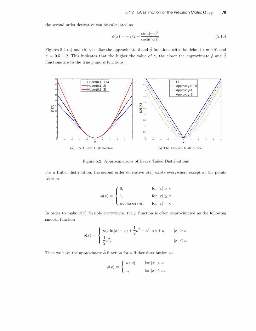
5.4.2 LA Estimation of the Precision Matrix G1:T |T 78
the second order derivative can be calculated as
φ(x) = −γ/2 +sinh(γx)2
cosh(γx)2(5.16)
Figures 5.2 (a) and (b) visualize the approximate ρ and φ functions with the default ǫ = 0.01 and
γ = 0.5, 1, 2. This indicates that the higher the value of γ, the closer the approximate ρ and φ
functions are to the true ρ and φ functions.
−5 −4 −3 −2 −1 0 1 2 3 4 50
2
4
6
8
10
12
14
16
18
20
22
x
ρ (x
)
Huber(0,1; 1.5)Huber(0,1; 2)Huber(0,1; 3)
(a) The Huber Distribution
−5 −4 −3 −2 −1 0 1 2 3 4 50
0.5
1
1.5
2
2.5
3
3.5
4
4.5
5
xab
s(x)
L1Approx: γ = 0.5Approx: γ=1Approx: γ=2
(b) The Laplace Distribution
Figure 5.2: Approximations of Heavy Tailed Distributions
For a Huber distribution, the second order derivative φ(x) exists everywhere except at the points
|x| = κ:
φ(x) =
0, for |x| > κ
1, for |x| ≤ κ
not existent, for |x| = κ
In order to make φ(x) feasible everywhere, the ρ function is often approximated as the following
smooth function
ρ(x) =
κ(x ln |x| − x) +1
2κ2 − κ2 lnκ+ κ, |x| > κ
1
2x2, |x| ≤ κ.
Then we have the approximate φ function for a Huber distribution as
φ(x) =
κ/|x|, for |x| > κ
1, for |x| ≤ κ.
5.5 Optimization Techniques 79
Figures 5.2 (a) and (b) visualize the approximate ρ and φ functions with different parameter settings
κ = 0.5, 1, 2,where the notation Huber(0, 1; 1.5) refers to a Huber distribution with a mean, variance,
and κ equal to 0, 1, and 1.5, respectively.
5.5 Optimization Techniques
This section presents two primal-dual optimization techniques for the RFR-STP algorithm when the
Huber or Laplace distribution is selected to model the measurement error.
5.5.1 Primal-Dual Optimization for Huber Distribution
This subsection explores the special structure of the R-STRE model based on the Huber distribution,
and presents a primal-dual interior point algorithm to achieve a close-to-linear-order time efficiency.
The Huber distribution is one of the most popular heavy tailed distributions used in robust statistics
[271]. In the R-STRE model, the Huber distribution is used to model the measurement error: the
random variable εt(sn,t) ∼ Huber(0, σε,t
√
vt(sn,t), κ). The pdf of the Huber distribution is defined
as p(ε;u, σ, κ) = 1σh(
ε−µσ ;κ), h(x;κ) = ce−ϕ(x;κ), and
ϕ(x;κ) =
κ|x| −1
2κ2, for |x| > κ
1
2x2, for |x| ≤ κ,
where c is a normalization constant to ensure that the integral∫
c/σe−ϕ(x;κ)dx = 1, and κ is a range
parameter of the distribution. The MAP optimization problem to be addressed is
minimizeη,ξ
1Tϕ(Z − OSη − Oξ) +1
2ηTMη + ETη
+1
2ξTΛξξ + const. (5.17)
Dual Problem
To derive a Lagrange dual of the primal problem stated in Equation (5.17), we first introduce a
new variable r and a new equality constraint r = Z − OSη − Oξ. The primal problem can be
reformulated as
minimizeη,ξ
1Tϕ(r) +1
2ηTMη + ETη +
1
2ξTΛξξ + const
subject to r = Z − OSη − Oξ
(5.18)
Associating an auxiliary variable ω with the equality constraint, we can derive the Lagrangian as
L(η, ξ, r,ω) = 1Tϕ(r) +1
2ηTMη + ETη +
1
2ξTΛξξ + ωT (r − Z + OSη + Oξ) + const.

5.5.1 Primal-Dual Optimization for Huber Distribution 80
Theorem 2 The dual function is
infη,ξ,r
L(η, ξ, r,ω) =
−ωT Z−1
2ωT O(SM−1ST + Λ−1
ξ )OTω − ωT OSM−1E −1
2ωTω + const, |ω| ≤ κ1
−∞, otherwise,
and
η = −M−1(ST OTω + E), (5.19)
ξ = −Λ−1ξ OTω. (5.20)
Proof See Appendix A.3.
Let G = O(SM−1ST + Λ−1ξ )OT + I. The dual problem can be reformulated as
minimizeω
ωT Z + ωT OSM−1E +1
2ωTGω + const
subject to ω − κ1 ≤ 0,−ω − κ1 ≤ 0.
(5.21)
Here, the condition “ω − κ1 ≤ 0” means that ωi − κ ≤ 0, ∀i. The above problem is a Quadratic
Programming (QP) problem with the variable ω. If it satisfies ω − κ1 ≤ 0 and −ω − κ1 ≤ 0,
the problem is said to be strictly dual feasible. After we have obtained the solution ω of the dual
problem stated in Equation (5.21), the primal variables η and ξ can be recovered via Equations
(5.19) and (5.20).
A Primal-Dual Interior-Point Method
The QP problem stated in Equation (5.21) can be solved by using standard numerical optimization
techniques such as deepest decent, Newton’s method, or interior point methods. This subsection
explores the special structure of the QP problem (5.21) by proposing a primal dual interior point
method. In the worst case, primal dual interior methods require a number of iterations equal to
O((∑
Nt)1/2). However, in practice this class of methods usually solves QP problems in a number of
steps that is independent of the data size. If the QP problem is processed correctly, the computation
cost is usually dominated by the cost of computing the search directions with time complexity
O(∑
Nt). Therefore, the total complexity is O(∑
Nt), which is the same as the time cost of the
traditional FR-STP approach.

5.5.1 Primal-Dual Optimization for Huber Distribution 81
The Lagrangian of problem (5.21) is
L(ω,λ1,λ2) = ωT Z + ωT OSM−1E +1
2ωTGω + λT
1 (ω − κ1) + λT2 (−ω − κ1) (5.22)
In order to select the search direction for the Newton step, we define the residual vector as
rt(ω,λ1,λ2) =
GTω + Z + OSM−1E + λ1 − λ2
−diag(λ1)(ω − κ1) − (1/t)1
−diag(λ2)(ω − κ1) − (1/t)1
,
where ω is primal feasible and λ1,λ2 are dual feasible, with a duality gap m/t. If ω,λ1,λ2 satisfy
rt(ω,λ1,λ2) = 0, then this is the optimal solution of problem (5.21). When t → ∞, the condition
rt(ω,λ1,λ2) = 0 degeneralizes to the standard Karush-Kuhn-Tucker (KKT) conditions for the dual
problem (5.21). The first component rdual is called the dual residual and the left two components
are centrality residuals. The basic idea of the primal dual interior point method is to iteratively
apply a Newton step to solve nonlinear Equations rt(ω,λ1,λ2) = 0 with increasing values of t.
Denote the current estimate and the Newton update as g = (ω,λ1,λ2) and ∆g = (∆ω,∆λ1,∆λ2),
respectively. The Newton step can be now represented by a system of linear equations
rt(g + ∆g) ≈ rt(g) +Drt(g)∆g = 0. (5.23)
In terms of ω, λ1, and λ2, we have
G I −I
−diag(λ1) −diag(ω − κ1) 0
diag(λ2) 0 diag(ω + κ1)
∆ω
∆λ1
∆λ2
= −
GTω + Z + OSM−1E + λ1 − λ2
−diag(λ1)(ω − κ1) − (1/t)1
−diag(λ2)(ω − κ1) − (1/t)1
The primal-dual search direction ∆gpd = (∆ω,∆λ1,∆λ2) is defined as the solution of the following
set of linear equations (5.24):
∆λ1 = −λ1 − diag(ω − κ1)−1
[
1
t1 + diag(λ1)∆ω
]
,
∆λ2 = −λ2 + diag(ω + κ1)−1
[
1
t1 + diag(λ2)∆ω)
]
,
∆ω = (B + D)−1
(−Bω + F) ,
B = OSM−1ST OT ,
D = OΛ−1ξ OT + I − diag(ω − κ1)−1diag(λ1) + diag(ω + κ1)−1diag(λ2), (5.24)
F = −OΛ−1ξ OTω − ω − Z − OSM−1E−
1
tdiag(κ1− ω)−11 +
1
tdiag(ω + κ1)−11.
5.5.2 Primal-Dual Optimization for Laplace Distribution 82
The primal-dual interior point algorithm is summarized in Algorithm 2.
5.5.2 Primal-Dual Optimization for Laplace Distribution
In this subsection, we consider how the Laplace distribution can be used to model the measurement
error. The Laplace distribution is another popular heavy tailed distribution that is widely used in ro-
bust statistics [271]. In the R-STRE model, the measurement error εt(sn,t) ∼ Laplace(0, σε,t
√
vt(sn,t)),
in which the pdf is defined as p(ε;u, σ) = 1σh(
ε−µσ ), and h(x) = 1
2e−|x|.
The MAP optimization problem to be solved is
minimizeη,ξ
∣
∣
∣Z − OSη − Oξ∣
∣
∣+1
2ηTMη + ETη +
1
2ξTΛξξ + const. (5.25)
To derive a Lagrange dual of the primal problem stated in Equation (5.25), we first introduce a new
variable r and a new equality constraint r = Z − OSη − Oξ. The primal problem (5.25) can be
reformulated as
minimizeη,ξ
1T |r| +1
2ηTMη + ETη +
1
2ξTΛξξ
subject to r = Z − OSη − Oξ
Associating an auxiliary variable ω with the equality constraint, we derive the Lagrangian as
L(η, r,ω) = 1T |r| +1
2ηTMη + ETη +
1
2ξTΛξξ + ωT (r − Z + OSη + Oξ).
Theorem 3 The dual function is
infη,r
L(η, r,ω) =
−1
2ωT O(SM−1ST + Λ−1
ξ )OTωωT Z− ωT OSM−1E + const, −1 ≤ ω ≤ 1 (5.26)
−∞, otherwise,
and
η = −M−1(ST OTω + E), (5.27)
ξ = −Λ−1ξ OTω. (5.28)
Proof See Appendix A.4.
By Theorem 3, the dual problem can be formalized as
minimizeω
ωT Z +1
2ωT O(SM−1ST + Λ−1
ξ )OTω + ωT OSM−1E + const
such that − 1 ≤ ω ≤ 1.
(5.29)
5.5.3 Time and Space Complexity Analysis 83
The above dual problem is a QP problem with the variable ω. If this satisfies −1 ≤ ω ≤ 1, the
problem is said to be strictly dual feasible. After we have obtained the solution ω of the dual
problem stated in Equation (5.29), the primal variable can be recovered via Equations (5.27) and
(5.28). An efficient primal-dual interior point algorithm can be designed, which has the same steps
as Algorithm 2 except for the formulas for calculating the components ω, λ1, and λ2. Readers are
referred to [236] for the detailed implementation.
5.5.3 Time and Space Complexity Analysis
This section evaluates the time and space complexity of the proposed RFR-STP-Huber algorithm,
which is designed based on interior point methods. Suppose the required number of interior point
iterations is L. As indicated in Algorithm 2, for each iteration the dominated time cost lies on the
calculation of the component ∆ω, which has the decomposition form
∆ω = (B + D)−1(−Bω + F).
The inversion of the matrix (B + D) can be calculated using the Sherman-Morrison-Woodbury
formula
(
OSM−1ST OT + D)−1
= D−1 − D−1OS(M + ST OTD−1OS)−1ST OTD−1.
Hence, the cost of inverting a square matrix of a large size (∑T
t=1Nt) is reduced to the cost of
inverting a square matrix of a much smaller size (Tr), and the time complexity is reduced from
O((∑T
t=1Nt)3) to O(
∑Tt=1Ntr
3). Note that the component (M + ST OTD−1OS) is sparse and the
inversion can be calculated using efficient solvers for sparse systems of linear equations. In practice,
the actual time cost is close to O(∑T
t=1Ntr3). Therefore, the total time cost of the proposed RFR-
STP-Huber algorithm is O(L∑T
t=1Ntr3). The total space cost is dominated by the required space
of the matrix (M + ST OTD−1OS), which takes O((∑T
t=1Nt)2). However, because this matrix is a
sparse matrix, the space cost of the compressed form reduces to O(∑T
t=1Nt ∗ r).
5.6 Experiments
This section focuses on the Huber distribution as a case study, and evaluates the robustness and effi-
ciency of the proposed RFR-STP based on both simulated and real-life data sets. All the experiments
were conducted on a PC with Intel(R) Core(TM) I7-Q740, CPU 1.73Ghz, and 8.00 GB memory.
The development tool was MATLAB 2011. Note that, we re-implemented all the competitive meth-
ods based on their original papers in our experiments, because the original implementations are
unavailable. Although we have strictly followed the rules of these papers, it is not guaranteed that
we have fully accurately implemented those methods and optimally tuned the related parameters.

5.6.1 Simulation Study 84
Figure 5.3: Experiment Design
As shown in Figure 6.4, the experimental design consisted of the following steps: 1) Data Prepro-
cessing, in which the raw data was reprocessed to obtain clean data Z, the log-transformation was
applied to Z such that the distribution was close-to-symmetric, and the study region selected; 2)
Parameter Estimation, in which the parameters of the STRE model were estimated based on Z
using the EM algorithm [259]; 3) Data Contamination, in which isolated or regional (cluster of)
outliers were added to the clean data Z to obtain the contaminated data Z; 4) Prediction, in which
the FR-STP was applied to Z to obtain the predicted Y, as the “true” Y, and then the FR-STP
and RFR-STP were applied to Z to predict Y; 5) Results Evaluation, where the mean absolute
percentage error (MAPE) and Root Mean Square Error (RMSE) between Y and Y were calculated:
MAPE =1
(∑T
t=1Nt)
T∑
t=1
Nt∑
n=1
|Ytn − Ytn|
Ytn
, (5.30)
RMSE =
1
(∑T
t=1Nt)
T∑
t=1
Nt∑
n=1
(Ytn − Ytn)2
12
. (5.31)
Subsection 5.6.1 presents a comprehensive simulation study, and Subsections 5.6.2 and 5.6.3 present
empirical evaluations based on two real-life datasets.
5.6.1 Simulation Study
This subsection presents a simulation study comparing the robustness of the proposed RFR-STP
approach with that the FR-STP approach. Here, we considered the same simulation model as that
used in the original FR-STP paper [228] to generate the simulated data.
1) Simulation Settings
The spatial domain was designed with one dimension and consisted of the observation locations
D = s : s = 1, · · · , 256. The temporal domain ranged from t = 1 to t = 100. The trend component
µt(s) was assumed identical to zero and the values Yt and Zt were simulated according to Equations
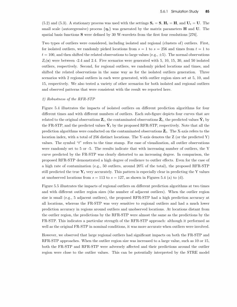
5.6.1 Simulation Study 85
(5.2) and (5.3). A stationary process was used with the settings St = S, Ht = H, and Ut = U. The
small scale (autoregressive) process ηt was generated by the matrix parameters H and U. The
spatial basis functions S were defined by 30 W-wavelets from the first four resolutions [276].
Two types of outliers were considered, including isolated and regional (clusters of) outliers. First,
for isolated outliers, we randomly picked locations from s = 1 to s = 256 and times from t = 1 to
t = 100, and then shifted the related observations to large values (e.g., ±5). The normal observations
Zt(s) were between -2.4 and 2.4. Five scenarios were generated with 5, 10, 15, 30, and 50 isolated
outliers, respectively. Second, for regional outliers, we randomly picked locations and times, and
shifted the related observations in the same way as for the isolated outliers generation. Three
scenarios with 2 regional outliers in each were generated, with outlier region sizes set at 5, 10, and
15, respectively. We also tested a variety of other scenarios for both isolated and regional outliers
and observed patterns that were consistent with the result we reported here.
2) Robustness of the RFR-STP
Figure 5.4 illustrates the impacts of isolated outliers on different prediction algorithms for four
different times and with different numbers of outliers. Each sub-figure depicts four curves that are
related to the original observations Zt, the contaminated observations Zt, the predicted values Yt by
the FR-STP, and the predicted values Yt by the proposed RFR-STP, respectively. Note that all the
prediction algorithms were conducted on the contaminated observations Zt. The X-axis refers to the
location index, with a total of 256 distinct locations. The Y-axis denotes the Z (or the predicted Y)
values. The symbol “t” refers to the time stamp. For ease of visualization, all outlier observations
were randomly set to 5 or -5. The results indicate that with increasing number of outliers, the Y
curve predicted by the FR-STP was clearly distorted to an increasing degree. In comparison, the
proposed RFR-STP demonstrated a high degree of resilience to outlier effects. Even for the case of
a high rate of contamination (e.g., 50 outliers, around 20% of the total), the proposed RFR-STP
still predicted the true Yt very accurately. This pattern is especially clear in predicting the Y values
at unobserved locations from s = 113 to s = 127, as shown in Figures 5.4 (a) to (d).
Figure 5.5 illustrates the impacts of regional outliers on different prediction algorithms at two times
and with different outlier region sizes (the number of adjacent outliers). When the outlier region
size is small (e.g., 5 adjacent outliers), the proposed RFR-STP had a high prediction accuracy at
all locations, whereas the FR-STP was very sensitive to regional outliers and had a much lower
prediction accuracy in regions around outliers and unobserved locations. At locations distant from
the outlier region, the predictions by the RFR-STP were almost the same as the predictions by the
FR-STP. This indicates a particular strength of the RFR-STP approach: although it performed as
well as the original FR-STP in nominal conditions, it was more accurate when outliers were involved.
However, we observed that large regional outliers had significant impacts on both the FR-STP and
RFR-STP approaches. When the outlier region size was increased to a large value, such as 10 or 15,
both the FR-STP and RFR-STP were adversely affected and their predictions around the outlier
region were close to the outlier values. This can be potentially interpreted by the STRE model

5.6.1 Simulation Study 86
assumptions (See Subsection 5.2.1) that define the spatio-temporal dependence between Z(si;u)
and Z(sj ; t), with i 6= j or u 6= t. In particular, the STRE model assumes a Gaussian process to
model the spatial dependence between Z(si; t) and Z(sj ; t), i 6= j, so observations will have a high
spatial correlation if they are spatially close. For the temporal dependence, the STRE model assumes
a first order autoregressive Markov process. That is, in addition to its dependence on observations
over other locations at time t, Zt is also dependent on its previous time observations Zt−1. Hence,
the STRE model considers a spatial Gaussian process, log-1 temporal autocorrelation, and white
noise (Gaussian distribution) to model the whole data variation. The proposed R-STRE model is
similar to the STRE model except that heavy tailed distributions such as the Huber and Laplace
distributions are utilized to model the white noise (the measurement error), instead of a Gaussian
distribution.
Spatio-temporal outliers can be interpreted as observations that have abnormally low correlations
with their spatio-temporal neighbors, considering normal deviations due to measurement error (white
noise). For the regular STRE model, when a data set has outliers the additional variation due to
those outliers will be captured by distorting the spatio-temporal dependence (or the sharpness of
the predicted Y curve). The white noise component is unable to handle large deviations due to
the light-tailed feature of the Gaussian distribution. This explains the distorted blue curves shown
in Figures 5.5 (a) and (b). A specific spatio-temporal autocorrelation pattern is associated with a
specific degree of sharpness of the resulting smoothed curves. In comparison, the proposed R-STRE
model uses heavy tailed distributions to model the measurement error. When outliers appear, the
proposed R-STRE model directly captures the additional large variation due to outliers as the
measurement error. When the outlier region becomes large, however, it becomes possible to use
normal spatio-temporal autocorrelations to directly capture the outlier variation. Intuitively, we are
able to use a smooth and unsharp curve to fit the observations well. This may explain why the
proposed RFR-STP failed to predict the correct Y values at locations close to the regional outliers
for large regional outliers.
2) Computational Efficiency of the RFR-STP
Table 5.1 compares the time cost for the RFR-STP and FR-STP approaches for different scenarios.
The results indicate that the optimized RFR-STP consistently achieved the same order of time
efficiency as FR-STP in all the scenarios tested. In contrast, the general RFR-STP had a time
efficiency that was around ten times lower than either the general FR-STP or the optimized RFR-
STP. One interpretation is that the optimized RFR-STP is a customized algorithm based on the
special structure of the Huber distribution, whereas the general FR-STP is a unified algorithm
designed for use with most existing heavy tailed distributions. Customized algorithms are usually
more efficient than non-customized algorithms. Considering that the FR-STP has a linear-order
time complexity, the general RFR-STP was still very fast, and should scale well with large datasets.
Note that the general RFR-STP was only compared with the optimized RFR-STP with regard to
time efficiency. As shown by Theorem 1, the RFR-STP is a strict convex problem for most existing
heavy tailed distributions, which implies that there exists a unique local (and global) optimum for
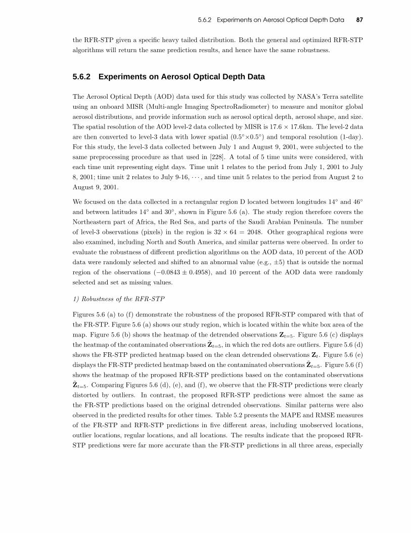
5.6.2 Experiments on Aerosol Optical Depth Data 87
the RFR-STP given a specific heavy tailed distribution. Both the general and optimized RFR-STP
algorithms will return the same prediction results, and hence have the same robustness.
5.6.2 Experiments on Aerosol Optical Depth Data
The Aerosol Optical Depth (AOD) data used for this study was collected by NASA’s Terra satellite
using an onboard MISR (Multi-angle Imaging SpectroRadiometer) to measure and monitor global
aerosol distributions, and provide information such as aerosol optical depth, aerosol shape, and size.
The spatial resolution of the AOD level-2 data collected by MISR is 17.6 × 17.6km. The level-2 data
are then converted to level-3 data with lower spatial (0.5×0.5) and temporal resolution (1-day).
For this study, the level-3 data collected between July 1 and August 9, 2001, were subjected to the
same preprocessing procedure as that used in [228]. A total of 5 time units were considered, with
each time unit representing eight days. Time unit 1 relates to the period from July 1, 2001 to July
8, 2001; time unit 2 relates to July 9-16, · · · , and time unit 5 relates to the period from August 2 to
August 9, 2001.
We focused on the data collected in a rectangular region D located between longitudes 14 and 46
and between latitudes 14 and 30, shown in Figure 5.6 (a). The study region therefore covers the
Northeastern part of Africa, the Red Sea, and parts of the Saudi Arabian Peninsula. The number
of level-3 observations (pixels) in the region is 32 × 64 = 2048. Other geographical regions were
also examined, including North and South America, and similar patterns were observed. In order to
evaluate the robustness of different prediction algorithms on the AOD data, 10 percent of the AOD
data were randomly selected and shifted to an abnormal value (e.g., ±5) that is outside the normal
region of the observations (−0.0843 ± 0.4958), and 10 percent of the AOD data were randomly
selected and set as missing values.
1) Robustness of the RFR-STP
Figures 5.6 (a) to (f) demonstrate the robustness of the proposed RFR-STP compared with that of
the FR-STP. Figure 5.6 (a) shows our study region, which is located within the white box area of the
map. Figure 5.6 (b) shows the heatmap of the detrended observations Zt=5. Figure 5.6 (c) displays
the heatmap of the contaminated observations Zt=5, in which the red dots are outliers. Figure 5.6 (d)
shows the FR-STP predicted heatmap based on the clean detrended observations Zt. Figure 5.6 (e)
displays the FR-STP predicted heatmap based on the contaminated observations Zt=5. Figure 5.6 (f)
shows the heatmap of the proposed RFR-STP predictions based on the contaminated observations
Zt=5. Comparing Figures 5.6 (d), (e), and (f), we observe that the FR-STP predictions were clearly
distorted by outliers. In contrast, the proposed RFR-STP predictions were almost the same as
the FR-STP predictions based on the original detrended observations. Similar patterns were also
observed in the predicted results for other times. Table 5.2 presents the MAPE and RMSE measures
of the FR-STP and RFR-STP predictions in five different areas, including unobserved locations,
outlier locations, regular locations, and all locations. The results indicate that the proposed RFR-
STP predictions were far more accurate than the FR-STP predictions in all three areas, especially

5.6.3 Experiments on Traffic Volume Data 88
the predictions at outlier locations.
2) Computational Efficiency of the RFR-STP
Table 1 compares the time cost for the the RFR-STP and FR-STP approaches. The results indicate
similar patterns as observed in the preceding simulation study. Both the general and the optimized
RFR-STP were computationally comparable to the FR-STP, and the optimized FR-STP had a much
higher computational efficiency than the general FR-STP algorithm. Similar patterns were observed
consistently on the traffic volume data set that will be discussed in the following subsection.
5.6.3 Experiments on Traffic Volume Data
The traffic volume data used here were collected in the downtown area of the city of Bellevue,
Washington (WA). A total of 105 detectors in this area were included in the modeling process. NE
8th Ave was selected as the test route because this is a major city corridor, with an annual average
weekday traffic of 37,700 veh/day. Data from 14 detectors, seven eastbound and seven westbound, on
NE 8th Ave were used to evaluate the robustness of different prediction algorithms. The evaluation
data were collected during the first week of June, 2007, and all data were aggregated into 5-minute
intervals to reduce the effect of random noise. Details of the preprocessing and model specification
are given in [294].
The X-axis refers to the timestamps from 5 am to 9 pm, and the Y-axis refers to the traffic volume,
aggregated at 5 minute intervals. Figure 5.7 (a) shows the traffic volume from detector #75 with
one significant spike of 1900 around 11 am, which was probably caused by a detector of malfunction.
On this detector, the FR-STP predictions exhibited a spike of over 800 triggered by the outlier.
However, the RFR-STP predictions had only a minor spike of around 550, which is a very reasonable
value. Figure 5.7 (b) shows the results for detector #215, with oscillating volumes throughout the
day. Because this detector was located close to detector #75 on the same route, the outlier on
detector #75 also affected the FR-STP predictions on detector #215. As can be observed from the
figure, the FR-STP predictions had a significant spike at exactly the same time the outlier appeared
on detector #75. In contrast, the RFR-STP predictions successfully limited the impact from the
spatially neighboring outlier to a reasonable value.
Another interesting observation shown in Figure 5.7 (b) is that most of the FR-STP predictions on
detector #215 were over-estimated, and the resulting curve predicted by the FR-STP failed to follow
the observation Z curve well. In contrast, the RFR-STP predictions were more accurate in most
locations. Although some of the RFR-STP predictions around 11AM were slightly over-estimated,
they were still more accurate than those of the FR-STP predictions. In addition, the RFR-STP
clearly limited the impacts of the outlier in a local temporal region, which provides a very good
demonstration of its robustness. One potential interpretation is that the FR-STP predictions were
conducted based on spatio-temporal autocorrelations captured by the STRE model. The outlier
observation on detector #75 around 11 am consequently had an impact on the predictions of both

5.6.3 Experiments on Traffic Volume Data 89
its spatial and temporal neighbors. The RFR-STP predictions were conducted based on the R-STRE
model, which is able to cope with large deviations caused by outliers as a part of the measurement
error by using a heavy tailed distribution. This feature limits the effect of outliers to a reasonable
value.

5.6.3 Experiments on Traffic Volume Data 90
ALGORITHM 1: A General RFR-STP Algorithm
input : Z1:T ,O1:T ,S1:T ,Vε,1:T ,Vξ,1:T ,Ψ
output: Y1:T |T
Calculate Z1:T , Z, O1:T , O, S,Λξ,1:T ,M,E by Equation (5.11);
Select initial values for η = [ηT1 , · · · , η
TT ]T and ξ1:T ;
Select a tolerance ǫ > 0;
repeatrepeat
Calculate the gradient and Hessian matrix for η:
b = −ST OTψ(Z − OSη − Oξ) + Mη + E;
P = ST OT Φ(Z − OSη − Oξ)OS + M;
Calculate the Newton step and decrement for η:
∆η = −P−1b; λ2η = bTP−1b;
Choose step size t by backtracking line search;
Update η = η + t∆η;
until λ2η/2 ≤ ǫ ;
for t = 1, · · · , T dorepeat
Calculate the gradient and Hessian matrix for ξt by Equations (10) and (11):
c = −OTt ψ(Zt − OtStηt − Otξt) + Λ
ξ,tξt;
R = OTt Φ(Zt − OtStηt − Otξt)Ot + Λ
ξ,t Compute the Newton step and
decrement for ξt:
∆ξt = −R−1c; λ2ξt
= cTR−1c;
Choose a step size t by backtracking line search;
Update ξt = ξt + t∆ξt;
until λ2ξt/2 ≤ ǫ ;
endUpdate λ2
η;
until λ2η ≤ ǫ, λ2
ξt≤ ǫT
t=1 ;
Calculate Y1:T |T by Equation (5.7)
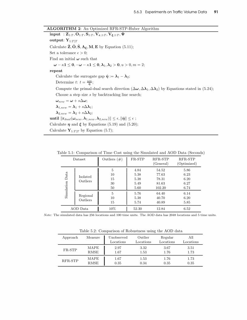
5.6.3 Experiments on Traffic Volume Data 91
ALGORITHM 2: An Optimized RFR-STP-Huber Algorithm
input : Z1:T ,O1:T ,S1:T ,Vε,1:T ,Vξ,1:T ,Ψ
output: Y1:T |T
Calculate Z, O, S,Λξ,M,E by Equation (5.11);
Set a tolerance ǫ > 0;
Find an initial ω such that
ω − κ1 ≤ 0,−ω − κ1 ≤ 0,λ1,λ2 > 0, u > 0,m = 2;
repeat
Calculate the surrogate gap η := λ1 − λ2;
Determine t: t = umη
;
Compute the primal-dual search direction (∆ω,∆λ1,∆λ2) by Equations stated in (5.24);
Choose a step size s by backtracking line search;
ωnew = ω + s∆ω;
λ1,new = λ1 + s∆λ1;
λ2,new = λ2 + s∆λ2;
until ‖rdual(ωnew,λ1,new,λ2,new)‖ ≤ ǫ, ‖η‖ ≤ ǫ ;
Calculate η and ξ by Equations (5.19) and (5.20);
Calculate Y1:T |T by Equation (5.7);
Table 5.1: Comparison of Time Cost using the Simulated and AOD Data (Seconds)
Dataset Outliers (#) FR-STP RFR-STP RFR-STP(General) (Optimized)
Sim
ula
tion
Data
IsolatedOutliers
5 4.84 54.52 5.8610 5.38 77.63 6.2315 5.38 78.31 6.2030 5.49 81.63 6.2750 5.60 102.20 6.74
RegionalOutliers
5 5.76 64.40 6.1410 5.38 40.70 6.2015 5.74 40.89 5.85
AOD Data 10% 52.30 12.84 6.52
Note: The simulated data has 256 locations and 100 time units. The AOD data has 2048 locations and 5 time units.
Table 5.2: Comparison of Robustness using the AOD data
Approach Measure Unobserved Outlier Regular AllLocations Locations Locations Locations
FR-STPMAPE 2.97 3.32 3.67 3.51RMSE 1.67 1.53 1.76 1.73
RFR-STPMAPE 1.67 1.53 1.76 1.73RMSE 0.35 0.34 0.35 0.35

5.6.3 Experiments on Traffic Volume Data 92
0 50 100 150 200 250
−4
−2
0
2
4
s
Observation Z Contaminated Z RFR−STP FR−STP
(a) t = 81, 10 outliers
0 50 100 150 200 250
−4
−2
0
2
4
s
(b) t = 17, 15 outliers
0 50 100 150 200 250
−4
−2
0
2
4
s
(c) t = 25, 30 outliers
0 50 100 150 200 250
−4
−2
0
2
4
s
(d) t = 63, 50 outliers
Figure 5.4: Comparison between the FR-STP and RFR-STP using the data observed at fourdifferent times and with different numbers of isolated outliers (15 unobserved locations from s =
113 to s = 127)

5.6.3 Experiments on Traffic Volume Data 93
0 50 100 150 200 250
−4
−2
0
2
4
s
Observation Z Contaminated Z RFR−STP FR−STP
(a) t = 8, 2 regional outliers of size 5
0 50 100 150 200 250−6
−4
−2
0
2
4
6
s
(b) t = 8, 2 regional outliers of size 15
Figure 5.5: Comparison between the FR-STP and RFR-STP using the data observed at twodifferent times and with different sizes of regional outliers (15 unobserved locations from s = 113 to
s = 127)
Longitude
Latit
ude
20 40 60 80 100 120 140 160 180
10
20
30
40
50
60
70
80
90
100
(a) Study Region
Longitude
Latit
ude
10 20 30 40 50 60
5
10
15
20
25
30
−1.5
−1
−0.5
0
0.5
1
1.5
(b) Detrended Observation Zt=5
Longitude
Latit
ude
10 20 30 40 50 60
5
10
15
20
25
30
−1.5
−1
−0.5
0
0.5
1
1.5
(c) Contaminated Zt=5
Longitude
Latit
ude
10 20 30 40 50 60
5
10
15
20
25
30
−1.5
−1
−0.5
0
0.5
1
1.5
(d) FR-STP Predictions on Zt=5
Longitude
Latit
ude
10 20 30 40 50 60
5
10
15
20
25
30
−1.5
−1
−0.5
0
0.5
1
1.5
(e) FR-STP Predictions on Zt=5
Longitude
Latit
ude
10 20 30 40 50 60
5
10
15
20
25
30
−1.5
−1
−0.5
0
0.5
1
1.5
(f) RFR-STP Predictions on Zt=5
Figure 5.6: Comparison between the FR-STP and RFR-STP on the contaminated AOD data setsobserved at time t = 5

5.6.3 Experiments on Traffic Volume Data 94
5 AM 7 AM 9 AM 11 AM 1 PM 3 PM 5 PM 7 PM 9PM0
500
1000
1500
2000
Time
Volu
me
Observation ZRFR−STP FR−STP
(a) t = 4th day, detector #75
5 AM 7 AM 9 AM 11 AM 1 PM 3 PM 5 PM 7 PM 9 PM0
200
400
600
800
1000
Time
Volu
me
Observation ZRFR−STP FR−STP
(b) t = 4th day, detector #215
Figure 5.7: Comparison between the FR-STP and RFR-STP using the Traffic Volume Data on the4th day. (Detectors #75 and #215 are spatial neighbors)

Chapter 6 95
Chapter 6
Application 1: ActivityAnalysis Based onLow Sample RateSmart Meters
Activity analysis disaggregates utility consumption from smart meters into specific usage that as-
sociates with human activities. It can not only help residents better manage their consumption
for sustainable lifestyle, but also allow utility managers to devise conservation programs. Existing
research efforts on disaggregating consumption focus on analyzing consumption features with high
sample rates (mainly between 1 Hz ∼ 1MHz). However, many smart meter deployments support
sample rates at most 1/900 Hz, which challenges activity analysis with occurrences of parallel activ-
ities, difficulty of aligning events, and lack of consumption features. We propose a novel statistical
framework for disaggregation on coarse granular smart meter readings by modeling fixture char-
acteristics, household behavior, and activity correlations. This framework has been implemented
into two approaches for different application scenarios, and has been deployed to serve over 300 pilot
households in Dubuque, IA. Interesting activity-level consumption patterns have been identified, and
the evaluation on both real and synthetic datasets has shown high accuracy on discovering washer
and shower.
This chapter is organized as follows: Section 2 illustrates the application deployment for the pro-
posed approach, and introduces the related challenges. A novel general statistical framework for
disaggregation is proposed in Section 3. The detailed implementations for water consumption disag-
gregation are described in Section 4. Section 5 evaluates the performance of the proposed approaches
under different scenarios with real-world and synthetic datasets and demonstrates some interesting
findings from the pilot households. The related work is reviewed in Section 6. Finally, Section 7
concludes our work with future directions.

6.1 Introduction 96
6.1 Introduction
Sustainability and design of sustainable technologies have become urgent and important priority for
cities given the unprecedented level of resource demand - water, energy, transit, healthcare, public
safety - to every imaginable service that makes a city attractive and desirable. At the same time,
digital reification of cyber-physical world has been possible with widespread penetration of sensing
and monitoring technologies. These two important catalysts have fuelled significant interest and cross
organizational collaboration among researchers, industries, urban planners, and government. A lot of
technology and research has recently focused on leveraging information from such digital reification
of cyber-physical world to help manage various services more efficiently. Our work takes a step
in that direction - examines the feasibility and provides innovative approaches towards influencing
people’s consumption behavior. More precisely, we provide activity analysis based on smart water
meter readings.
Given the real world constraints, we research the feasibility of activity analysis to identify activities
from smart utility meter readings. Our study is based on the hypothesis that consumption activities
disaggregated from meter readings will empower residents with appropriate insights to influence and
shape their behavior. This has been rightly validated through a city-wide survey [233] followed by
four-month-long experimentation with a real city [293]. In addition, from disaggregated consump-
tion, utility managers can design and assess conservation programs, and prioritize energy-saving
potential retrofits.
Research on disaggregating electricity or water load has been conducted on smart meter readings with
fine granularity (mainly between 1 Hz ∼ 1MHz). Existing approaches identify appliances (fixtures)
based on analyzing steady state or transient state change in real-time consumption. However, they
are not suitable for many existing smart meter infrastructure.
Real-world deployments of smart meters are designed for utility billing and some basic analysis
requirement, but many of them are not suitable for consumption disaggregation. Smart meters
transmit consumption readings using wireless protocols, which consume battery and have depen-
dency on physical environments. Although the meters can sample at a rate even higher than 1MHz,
many of existing deployments have chosen to accumulate to 15 min or even longer intervals to ensure
reliable data transmission. However, physical environment may still affect the data transmission.
This scenario brings the following challenges to consumption disaggregation: 1) Parallel usage ac-
tivities, e.g., a toilet flush and shower in the same 15 minute interval. 2) Difficulty of aligning usage
events temporally, e.g., a shower may appear in one or two intervals. 3) Lack of features, i.e., only
aggregated consumption and start time of each interval can be used to identify usage activity. An
example of such water meter data and expected disaggregated activities is illustrated in Figure 6.1.
To handle these challenges, we have designed a novel statistical framework for activity analysis
on coarse granular smart water meter readings, and deployed it as a component in Smarter Wa-
ter Service for Dubuque, IA. In this framework, fixture characteristics, household behavior, and
activity correlations are utilized to disaggregate consumption. To implement this framework, we

6.2 Background 97
Figure 6.1: An Example of Data and Disaggregated Activities
propose two approaches to identify activities. The first approach applies hidden Markov model to
capture the relationship among consumption events and hidden activities. The second approach
utilizes classification techniques to learn from labeled activities, and a Gaussian mixture model is
used for disaggregation. The proposed approaches have been validated using both real-world water
consumption and synthetic datasets. The experiments have demonstrated the capability of the pro-
posed disaggregation framework, illustrated the appropriate sample rate for disaggregation in various
applications, and revealed interesting usage insights from 300+ pilot households. In summary, the
major contributions of this work include:
• Providing activity-level consumption insights to residents and the city management team to
support decision making;
• Designing a general disaggregation framework with two implementations for different scenarios;
• Designing a general disaggregation framework with two implementations for different scenarios;
• Revealing interesting consumption patterns from the disaggregation results.
6.2 Background
The activity analysis is an important function provided in Smarter Water Service based on smart
water meters. The deployed environment of our smart water meter infrastructure is shown in
Figure 6.2. Since August 2010, over 300 pilot households have volunteered to install Neptune R900
smart water meters [274] with UFR (Unmeasured Flow Reducer), which transmit a new aggregated
reading roughly every 15 minutes through 900MHz wireless connection. Each aggregated reading
is broadcasted repeatedly within the entire interval to ensure the success of transmission. Wireless
gateways have been deployed in the city to collect these readings, attach timestamps, and send to
a data center through 3G network every hour. In addition, 6 volunteer households had applied

6.2 Background 98
data logger which records water consumption every 10 seconds, and had done water usage activity
journaling accordingly for a week. All the meter readings have been anonymized and sent to IBM
Computing Cloud for analytics.
Figure 6.2: Data Acquisition
The software architecture of the deployment is visualized in Figure 6.3. The smart meter data are
first cleaned and transformed by InfoSphere Information Server (IIS), and then stored in a Smart
Meter Database managed by DB2 . On top of this database, Cognos is utilized to provide OLAP
functions such as consumption metric and pattern monitoring; a java-based module is developed to
perform advanced analytics functions such as disaggregation and prediction. IBM WebSphere Ap-
plication Server (WAS) hosts the service layer to allow users interact with the services. In addition,
a community engagement component plays the role of motivating residents through competition and
collaboration via multiple media channels. The whole system, as a $850K deployment engagement
with Dubuque, IA, has been deployed on IBM Smarter Cities Sustainable Model Cloud, and provides
services to residents (300+ pilot households) and the city management team (about 10 government
employees) [293].
The main objective of this Smarter Water Service is to provide affective services that can help the
volunteers modify their behavior to be more sustainable, in other words, let the residents know
what they need to know to change their behavior. To achieve that goal, one important process is
to reveal disaggregated water consumption, so that the users can know where in their houses they
could conserve water, and sustainable operations or investment can be suggested. As a component
of Smarter Water Service, activity analysis shared the computing resources with the other custom
analytics. It works as a backend service that outputs activity-level consumption distribution reports
every month from 15-minute aggregated consumption. This component will continuously provide
consumption insights as part of the Smarter Water Service, and will be updated by enhancing
learning ability and expanded to the expected 4000 households with hourly readings by 2013.
A preliminary summary has shown 6.6% normalized accumulative consumption reduction in 8 weeks
after the Smarter Water Service was published in September 2010. In addition, a survey conducted
in December 2010 showed that since September, out of 64 respondents, 15 households had fixed leaks,

6.2.1 Problem and Definition 99
Figure 6.3: Smarter Water Service Architecture
13 respondents had shortened their showers, and 14 purchases on water-efficient toilet/appliances
had been made.
6.2.1 Problem and Definition
The problem of disaggregation from coarse granular smart water meter readings can be informally
described as follows:
Definition 1 (Disaggregation) Given a sequence of aggregated interval water consumption Con(T ) =
(Con1, · · · , ConT ), where Coni refers to the aggregated water consumption at the i-th time interval,
the proposed solution should return a set of activities ((A1, E1), · · · , (Ak, Ek)) that are most likely to
cause the aggregated consumption Con(T ), where Ai refers to an activity state (e.g., washer, shower,
or toilet uses), and Ei refers to an observation (event) of water consumption for this activity state
and is represented by a vector of event features, including total water consumption and start/end
time intervals.
The related terms and their definitions are summarized in Table 1, and will be used in the rest of the
chapter. We use capital letters to denote random variables and small letters to denote observations.
6.2.2 Research Challenges
General challenges for usage disaggregation from single main meter include the following: 1) Ap-
pliances (fixtures) with similar consumption patterns, e.g., certain sink usage and a toilet flush; 2)
Appliances/fixtures with multiple settings, e.g., normal, dedicated, and permanent of a washer; 3)
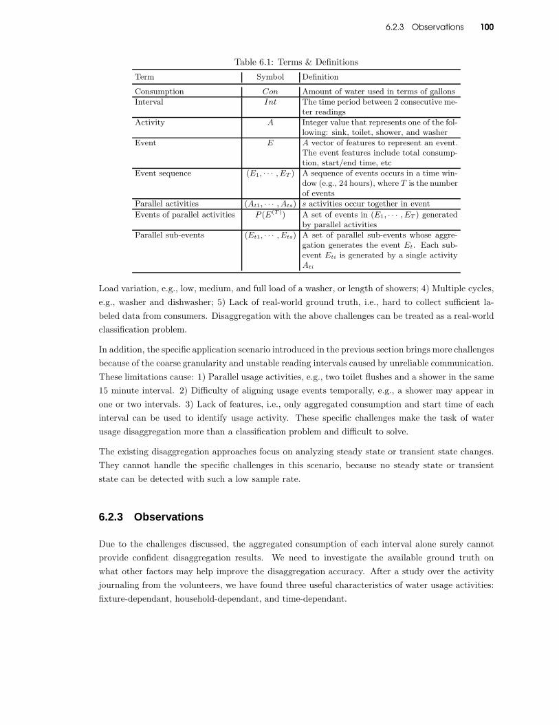
6.2.3 Observations 100
Table 6.1: Terms & Definitions
Term Symbol Definition
Consumption Con Amount of water used in terms of gallons
Interval Int The time period between 2 consecutive me-ter readings
Activity A Integer value that represents one of the fol-lowing: sink, toilet, shower, and washer
Event E A vector of features to represent an event.The event features include total consump-tion, start/end time, etc
Event sequence (E1, · · · , ET ) A sequence of events occurs in a time win-dow (e.g., 24 hours), where T is the numberof events
Parallel activities (At1, · · · , Ats) s activities occur together in event
Events of parallel activities P (E(T )) A set of events in (E1, · · · , ET ) generatedby parallel activities
Parallel sub-events (Et1, · · · , Ets) A set of parallel sub-events whose aggre-gation generates the event Et. Each sub-event Eti is generated by a single activityAti
Load variation, e.g., low, medium, and full load of a washer, or length of showers; 4) Multiple cycles,
e.g., washer and dishwasher; 5) Lack of real-world ground truth, i.e., hard to collect sufficient la-
beled data from consumers. Disaggregation with the above challenges can be treated as a real-world
classification problem.
In addition, the specific application scenario introduced in the previous section brings more challenges
because of the coarse granularity and unstable reading intervals caused by unreliable communication.
These limitations cause: 1) Parallel usage activities, e.g., two toilet flushes and a shower in the same
15 minute interval. 2) Difficulty of aligning usage events temporally, e.g., a shower may appear in
one or two intervals. 3) Lack of features, i.e., only aggregated consumption and start time of each
interval can be used to identify usage activity. These specific challenges make the task of water
usage disaggregation more than a classification problem and difficult to solve.
The existing disaggregation approaches focus on analyzing steady state or transient state changes.
They cannot handle the specific challenges in this scenario, because no steady state or transient
state can be detected with such a low sample rate.
6.2.3 Observations
Due to the challenges discussed, the aggregated consumption of each interval alone surely cannot
provide confident disaggregation results. We need to investigate the available ground truth on
what other factors may help improve the disaggregation accuracy. After a study over the activity
journaling from the volunteers, we have found three useful characteristics of water usage activities:
fixture-dependant, household-dependant, and time-dependant.

6.3 A NEW STATISTICAL DISAGGREGATION FRAMEWORK 101
Observations
Each fixture category has its own usage pattern in term of consumption and duration that can be
used to distinguish it from the others. Specifically, the amount of water consumed in a toilet flush
usually fell in several small ranges between 1.5 5 gallons, and was consistent for a specific toilet. A
load of washer generally lasted between 30 60 minutes, and consisted of multiple cycles with similar
water usage. Showers had consistent flow rate most of the time, and lasted from 5 minutes to 15
minutes in most cases. Sink usage was usually short in time and low in consumption. These patterns
can help briefly categorize the usage events. For example, any interval with flow rate lower than 0.1
gallons per 15 minutes can be filtered out as sink usage. However, using a fixture specification library
is not enough to identify parallel activities, or to deliver customized models for each household.
Household-dependant Pattern
Activity patterns heavily depend on the fixture models and occupants of a specific household. For
example, households with kids generally spent more time on shower every day; households with
open leaks showed continuous usage for a long time; some households have 3 toilets and each has a
different specification. Therefore, each household needs to be modeled separately to ensure accurate
disaggregation. These models can be learned from historical consumption records and household
profiles if available.
Time-dependant Pattern
According to human behavior, some activities may happen frequently during a specific time period,
which can be used to distinguish ambitious water usage. One interesting example of such pattern is
shower. Most of the labeled showers happened either close to the first event of usage in the morning
or close to the first event after work. Although toilet flush occurred almost any time in a day, it
was less frequent in working hours and midnight than the rest of a day. Not only time of day, but
also day of week has been found drawing impacts on activity patterns. An example could be washer
usage which happened mostly during weekends in some households. In addition, some activities are
found temporally associated. For instance, a toilet flush in many cases was followed by a short sink
usage for hand washing. According to the time-dependant activity patterns, timestamps of usage
events should be able to improve disaggregation results significantly.
6.3 A NEW STATISTICAL DISAGGREGATION FRAMEWORK
Coarse granular smart meter readings cause a large portion of parallel activities, and disaggregation
of parallel activities has become a critical and important challenge. This section introduces a new
General Disaggregation Framework (GDF) to address the disaggregation problem. As illustrated in

6.3 A NEW STATISTICAL DISAGGREGATION FRAMEWORK 102
Figure 6.4, the GDF framework applies six phases to disaggregate water consumption. The work
flow is described as follows:
Figure 6.4: Disaggregation Framework
Phase 1 Event extraction: Given a sequence of aggregated interval consumption Con(T ) =
(Con1, · · · , ConT ), the intervals with continuous consumption are grouped to generate events where
each represents one activity or parallel activities. The output of this phase is an event observation
sequence of a given time window: e(T ) = (e1, e2, · · · , eT ). Hence, e(T ) is regarded as one observation
of the event random variables E(T ) = (E1, E2, · · · , ET ). Each event Ei may be generated by a
hidden activity (Ai) or several parallel hidden activities (Ai1, · · · , Ais).
Phase 2 Model selection and training: Select an appropriate stochastic model D(E(T ); θ), such
as HMM or GMM, and estimate parameters θ based on historical labeled or unlabeled observations.
Phase 3 Parallel activity detection: Given the estimated stochastic model D(E(T ); θ), the
events with parallel activities P(e(T )) can be identified from anomalous events O(e(T )). Anomalous
events can be obtained using leave-one-out test, i.e., O(e(T )) = et|et ∈ R(E(−t) = e(−t), α),
where E(−t) = (E1, · · · , Et−1, Et+1, · · · , ET ), e(−t) = (e1, · · · , et−1, et+1, · · · , eT ). R(·) refers to
the outlying region of normal event Et that is defined based on the conditional distribution of
[Et|E(−t) = e(−t)] and a confidence level α (e.g., 0.99). The calculation of outlying regions based on
HMM and GMM models will be discussed in Section 4. This phase assumes all anomalous events are
generated due to parallel activities. An anomalous event may also be generated by true abnormal
activities such as a shower lasting more than an hour. However, it is difficult to differentiate these
only based on coarse granular meter readings. Hence, we only consider parallel activities.
Phase 4 Parallel size estimation: For each anomalous event observation et ∈ O(e(T )), the
number of parallel activities that generate et can be estimated by
s = mins|et ∈ R−Agg(E
(−t) = e(−t), Agg(Et1, · · · , Ets), α) (6.1)
where Et1, · · · , Ets refers to the parallel activities (random variables) whose aggregation generates
the event et, Agg(·) refers to the vector of aggregated features, and R−Agg(·) refers to the normal
region of the aggregated features Agg(Et1, · · · , Ets).Agg(Et1, · · · , Ets) returns aggregated features,
such as the total water consumption, the earliest start time, and the latest end time of the sub-events

6.4 DISAGGREGATION APPROACHES 103
Et1, · · · , Ets. The reason of selecting the minimal s is that heavy consumption (a washer load)
can always be decomposed into a large number of small activities (e.g., toilet flushes), which is not
reasonable.
Phase 5 Hidden activity identification: For each abnormal event Et ∈ O(ET ), given s, the
estimated size of parallel activities, this phase estimates the disaggregated activities
(at1, · · · , ats) = argmin(at1,··· ,ats)∈1,··· ,ms
Pr(At1 = at1, · · · , Ats = ats|E(−t) = e(−t),
Agg(Et1, · · · , Ets) = et). (6.2)
Phase 6 Consumption decomposition: Given the hidden parallel activities at1, · · · , ats esti-
mated in Phase 5, the related water consumption of these hidden activities can be estimated as:
(Con(et1), · · · , Con(ets)) = argmax(Con(et1),··· ,Con(ets))
L(Con(Et1) = Con(et1), · · · , Con(Ets)
= Con(ets)|E(−t) = e(−t), At1 = at1, · · · , Atm = ats,
Agg(Et1, · · · , Ets) = et), (6.3)
where L is the likelihood function, and Con(eti) is the consumption feature of the sub-event obser-
vation eti, i = 1, · · · , s.
Theorem 4 Given a sequence of aggregated consumption intervals Con(T ) = (Con1, · · · , ConT ),
GDF is able to identify true hidden activities ((A1, E1), · · · , (Ak, Ek)) of Con(T ), if the following
assumptions are satisfied: a) In Phase 1, The events can be correctly identified and the features
extracted are sufficient; b) The distribution D(E(T );θ) is correctly selected and estimated; c) All
anomalous events are due to parallel activities; d) The minimal s selected in Phase 4 is correct.
Proof The four conditions stated above assure that the built statistical model by GDF is consistent
with the true distribution of hidden activities of Con(T ). It follows that the activities identified by
GDF are most probable results and should be consistent with true hidden activities.
6.4 DISAGGREGATION APPROACHES
This section presents two approaches based on GDF to handle different disaggregation scenarios.
When there is no sufficient training data available, which is true in many real-world scenarios, we
propose an approach to learn hidden relationship among consumption events and activities without
user input based on hidden Markov model (HMM). When labeled activities are available for training,
we design the second approach to construct statistical models using classification techniques and
disaggregate parallel activities using Gaussian mixture model (GMM).

6.4.1 HMM-based Approach 104
6.4.1 HMM-based Approach
This section presents an implementation of GDF based on HMM. It is trained based on unlabeled
data and performs disaggregation without user input. For the purpose of simplicity, each event Ei
is represented by a single feature, the total water consumption. Other features, such as start/end
time intervals, and duration can be included to this approach in a straightforward manner.
Event Extraction (GDF Phase 1)
The key challenge of event extraction is the segmentation process. Without labeled historical data,
it is necessary to define a set of heuristic rules to generate meaningful events based on domain
knowledge. The basic criterion is to keep adjacent interval consumption in a single event if they
possibly relate to one activity or parallel activities. This is to avoid the situation where one activity is
divided to two separate events, which is not recoverable in our approach. If two nonparallel activities
are mistakenly grouped to one event, they can still be identified in the consequent disaggregation
process.
Similar to the idea of hierarchical clustering, a bottom-up based segmentation algorithm is proposed
as follows:
1. Preprocessing. Remove leaking effects, and filter out all zero-consumption intervals.
2. Initialization. Regard each left interval as one event. Then we have the sequence of initial
events (e1, , ek), where k is the number of nonzero consumption intervals.
3. Merging heavy events. Define a water consumption threshold ϑ (e.g., 5.5 gallons for 15-minute-
size intervals). For each continuous event pair (ei, ei+1), if Con(ei) > ϑ andCon(ei) > ϑ, merge
ei and ei+1. Repeat until no such pair exists.
4. Merging light events. For each event ei with Con(ei) > ϑ, if Con(ei−1) > 0, then merge ei
and ei−1. Similarly, if Con(ei+1) > 0, then merge ei and ei+1. If there is an event ei with
Con(ei) > 0, and both Con(ei−1) and Con(ei+1) greater than ϑ, then ei is merged to the
segment with the smallest consumption.
5. Merging peak events, Merge two peak events (Con(ei), Con(ej)) if dist(ei, ej) ≤ τ , where
dist(ei, ej) = tstart(ej)− tend(ei), and tstart(·) and tend(·) refer to the start and end time of an
event respectively. We define an event as a peak if its total water consumption is greater than a
threshold γ (e.g., 20 gallons). This step is specifically designed for fixtures like washers, which
consists of multiple peaks with more than 15 minutes empty cycle (no water consumption)
between peaks.

6.4.1 HMM-based Approach 105
HMM Parameter Estimation (GDF Phase 2)
A hidden Markov model is usually trained based on EM algorithm, which can only guarantee local
optimum. Given a large number of parameters to be estimated in a HMM model, including the
number of hidden states, the initial probabilities, the emission distribution of each state, and the
transition matrix, it is critical to find appropriate initial settings for these parameters. By empirical
evaluation, we decided a mixture model of three Gaussians for sink events, and Gaussian models for
other activity events. This section presents a heuristic based approach to seek initial settings for
each household based on generic domain knowledge:
1. Toilet identification. Hierarchical clustering is applied on events to identify toilet clusters. By
domain knowledge, toilet clusters could be identified by requiring the cluster size to be greater
than 3 times the total number of days in the training data, and the consumption standard
deviation smaller than 0.5 gallons.
2. Sink identification. Sink events can be identified as the events with consumption lower than
(µi − 2 ∗ σi), where µi and σi are the mean and standard deviation of the toilet cluster with
the smallest mean consumption in all toilet clusters.
3. Frequent pattern identification. After removing sink events and toilet clusters, hierarchical
clustering is applied on the remaining events to identify other qualified clusters. In order to
control the HMM complexity, we only keep the 12 clusters with the smallest standard deviation.
4. Cluster labeling. This step gives labels to the qualified clusters based on predefined rules such
as a shower usage should be within 5 ∼ 25 gallons. If some clusters are still not labeled, we
label these clusters as ”others”, which may relate to some unknown activity state or frequent
combination of parallel activities.
5. Anomaly removal. The anomalous events are identified based on a Gaussian mixture distri-
bution estimated from qualified clusters. These outliers will impact the training of HMM,
therefore they are removed from training data.
6. Probability estimation. Regarding each qualified cluster as a hidden state, we can get the
number of hidden states, the mean and standard deviation of each hidden state. The transition
matrix and initial probabilities can be estimated based on labeled events.
Disaggregation and Labeling (GDF Phase 3-6)
First, several notations are defined as follows. The set of activity states is 1, ,m, D is an m by
m transition matrix, π is the initial probability of the m states, pi(et) = Pr(Et = et|At = i), and
ui(t) = Pr(At = i). For the purpose of simplicity, we assume that each event Et conditioned on
activity state At follows a Gaussian distribution [EtAt = i] ∼ N (µi, σ2i ). Note that the following
derivations can also be straightforwardly extended to Gaussian mixture distributions.

6.4.1 HMM-based Approach 106
Let P (e) =
p1(e) 0 0
0 · · · 0
0 0 ps(e)
∈ Rs×s, αt = Pr(e1, . . . , et, At) ∈ Rs, αt(at) = αt = Pr(e1, . . . , et, At =
at) ∈ R, βt = Pr(et+1, . . . , eT |At) ∈ Rs, βt(at) = Pr(et+1, . . . , eT |At = at) ∈ R, and Bt = DP (et).
The HMM implementations of GDF Phase 3 to 6 are as follows:
GDF Phase 3: Parallel activity detection
The probability density function
P (Et = e|E(−t) = e(−t)) =αT
t−1DP (e)βt
αTt−1Dβt
=∑
i
wi(t)pi(e),
where wi(t) = di(t)∑
mj=1 dj(t)
, di(t) = [αTt−1D]i[βt]i. It indicates that [Et = e|E(−t) = e(−t)] follows a
GMM :
[Et = e|E(−t) = e(−t)] ∼∑
i
wi(t)N (x|µi, σ2i ).
The outlying region of the GMM model can be calculated as
R(e(−t), α) =
e∣
∣
∣|e− µk∗ | > σk∗Φ−1(
1 − α
2)
,
where k∗ is the Gaussian component closest to e, and Φ(·) is the cumulative density function (CDF)
of a standard Gaussian distribution. Here, we assume that the statistics of outlying events are
dominated by the component closest to the observation. This outlying region estimation has been
justified in [281] using extreme value statistics.
GDF Phase 4: Parallel size estimation
The probability density function
P (Et1 = et1, . . . , Ets = ets|e(−t)) =
αTt−1
∏si−1 DP (eti)βt
αTt−1D
sβt
=∑
(l1,...,ls)∈1,...,ms
wl1,...,lsPls(et1) · · ·Plm(ets),
where wl1,...,lm is the weight that can be calculated based on the form αTt−1 ·
∏si=1DP (eti) · βt/α
Tt−1D
sβt.
It implies that
[Et1, . . . , Ets|E(−t) = e(−t)] ∼
∑
(l1,...,ls)∈1,...,ms
wl1,...,lsN(
[µl1 , . . . , µls ]T , diag(σ2
l1 , . . . , σ2ls))
.

6.4.2 Classification-GMM-based Approach 107
By linear transformation, we have that
[Et1 + · · · + Ets|E(−t) = e(−t)] ∼
∑
(l1,...,ls)∈1,...,ms
wl1,...,lsN(
s∑
k=1
µli ,
s∑
k=1
σ2li
)
.
Note that here Agg(Et1, . . . , Etm) = Et1 + · · · + Ets. Since [Agg(Et1, . . . , Etm)∣
∣ E(−t) = e(−t)]
follows a Gaussian Mixture distribution, the normal region R−Agg(·) can be estimated similarly as in
the above GDF Phase 3.
GDF Phase 5: Hidden activity identification
The probability density function
Pr(At1 = at1, . . . , Ats = ats
∣
∣ E(−t) = e(−t), Et1 + · · · + Ets = et)
=αt1(at1)
∏s−1i=1 Pr(at(i+1)|ati)Pr(
∑
k Etk = et|at1, . . . , ats)βts(ats)
LT
where LT is the likelihood of the whole sequence and can be neglected when solving the problem
(6.2). Note that the random variables Et1, . . . , Ets are independent to each other given their hidden
activity states At1, . . . , Ats. The probability density function Pr(∑
k Etk = et | at1, . . . , ats) can be
calculated by simple linear transformation of independent Gaussian random variables.
GDF Phase 6: Consumption decomposition
Given the hidden activity states at1, . . . , ats, we have that
[Et1, . . . , Ets|at1, . . . , ats] ∼ N (µ,Σ),
where µ = [µat1 , . . . , µats]T ,Σ = diag(σ2
t1, . . . , σ2ats
). The optimal solution of the problem (6.3) can
be obtained as [282]
[et1, . . . , ets]T = µ− Σ−11T(1TΣ1)−1(1Tµ− et).
6.4.2 Classification-GMM-based Approach
Different from the HMM -based approach, this section presents a mixed model approach to the
disaggregation problem that requires labeled data for training. It first applies a classification model
(e.g., support vector machine, neural network, and k-nearest neighbor classifier) to classify each
event as a single activity, or a known frequent combination of parallel activities, or an unknown
infrequent combination of parallel activities. For the events classified to the last category (unknown
infrequent combinations), it applies an implementation of the GDF framework based on GMM to
disaggregate parallel activities.
Assume that we are given a sequence of aggregated interval consumption Con(T1) = (Con∗1, . . . , Con
∗T1
)
and the related hidden activities(
(a∗1, e∗1), . . . , (a
∗k, e
∗k))
as the labeled training data. The objective

6.4.2 Classification-GMM-based Approach 108
is to build a model on Con(T1) that can identify unknown hidden activities(
(a1, e1), . . . , (ak, ek))
of a new aggregated intervals consumption sequence Con(T ) = (Con1, . . . , ConT ).
Event Extraction (GDF Phase 1)
This phase first applies the same procedure as in Section 3.2.1 to identify a sequence of events. Here
each ei has six features, which include the start time, duration, total consumption, minimal interval
consumption, maximal interval consumption, and number of peaks.
Classification (GDF Phase 2)
The event extraction phase returns an event sequence (e1, . . . , ek), where each ei is represented by a
vector of six features (ei ∈ R6). Note that all the features are mapped to real type values, in order
to apply classification models such as SVM and neural network.
Here, we neglect the dependencies between events and treat (e1, . . . , ek) as a set of independent
training instances: e1, . . . , ek. Based on the labels (a∗1, e∗1), . . . , (a
∗k, e
∗k), it is able to identify hidden
activities of each event ei. To decide class labels, not only single activities (e.g., toilet, shower, and
washer) are treated as distinct classes, but also frequent combinations of parallel activities are
regarded as distinct classes. The current setting is that frequent parallel activities should occur at
least once per week.
GMM-based Disaggregation (GDF Phase 3-6)
After the classification process, each event has been labeled as a single activity, or known/unknown
combination of parallel activities. For parallel activities, a GMM -based implementation of the GDF
framework is proposed to disaggregate parallel activities. The basic procedures are as follows:
Based on the labels of training events e1, . . . , ek, it is able to collect training instances for each
activity state, such as toilet, shower, and washer. For simplicity, in this disaggregation step, we
only consider a single feature (the total water consumption), for each event ei. Each single-activity
related event (Et) can modeled by a Gaussian mixture distribution as Et ∼∑m
i=1 πiN (µi, σ2i ), where
πi is the prior probability of the activity state i, and N (µi, σ2i ) is the event distribution of activity
i.
Given an event et that is classified as parallel activities, the objective is to identify the most probable
hidden activities(
(at1, et1), . . . , (ats, ets))
with Agg(et1, . . . , ets) = et. Here the aggregation function
Agg is the summation function∑
(·). The GDF disaggregation framework can be employed here,
which can be regarded a simplified case of HMM based approach. Readers are referred to [261] for
detailed specifications.

6.5 Evaluation & Findings 109
6.5 Evaluation & Findings
The framework has been implemented using JDK 1.5 and deployed in the Custom Analytics Layer
of the Smarter Water Service (Figure 6.4). Pie charts of activity consumption distribution are
generated to illustrate how each fixture has been used on monthly basis. From the Smarter Water
Service layer interface, the residents can browse their own consumption distribution; meanwhile, the
government agency and utility manager can explore how water has been consumed by each activity
at regional level.
Both HMM-based and GMM-based approaches have been implemented and evaluated. Specifically,
for the GMM-based approach, we have assessed three classification methods, k-Nearest Neighbor
classification (kNN-GMM), Artificial Neural Network (ANN-GMM), and Support Vector Machine
(SVM-GMM) accordingly. Given the available labeled activities, the evaluation focused on identi-
fying toilet flushes, showers, and washer loads.
To evaluate the effectiveness of consumption disaggregation on identifying these activities, we
adopted three metrics, precision, recall, and F-measure. The major reason of using these metrics is
that the disaggregation evaluation is similar to an information retrieval process, where subsets of
intervals represent certain true activities and the testing results are also subsets of intervals labeled
as activities. The metrics need to capture not only how many labels are matched, but also how many
true activities are missed and how many false labels are placed. These metrics are defined as follows:
Precision refers to the portion of matched activities within the corresponding disaggregation results;
Recall refers to the portion of matched activities within the corresponding true activities; F-measure
is the harmonic mean of precision and recall.
To evaluate the proposed disaggregation solution, we have applied both HMM-based and GMM-
based approaches on the consumption of 6 volunteer households, as well as 50 simulation datasets
that were generated based on their labeled consumption. In addition, we varied the sample rate in
these datasets to investigate its impact on disaggregation results. The correlation between sample
rate and effectiveness can provide guidance to future planning and deployment of human activity
analysis applications.
Due to the lack of labeled activities from most of the pilot households, we only applied the HMM-
based model to analyze activities of the 300+ pilot households. Some interesting patterns discovered
can illustrate common human behavior characteristics.
6.5.1 Datasets
A real-world dataset was collected from 6 volunteer households. It consists of 1/10 Hz water reading
and the corresponding usage journaling records for 7 days. The usage journaling was input manually
by these volunteers, so it always has approximated timestamps and missing activities, which intro-
duce inaccuracy which needs to be handled carefully. Note that these households came from various
demographic categories and showed significantly different consumption patterns. A summary of

6.5.2 Parameter Settings & Baseline Methods 110
Table 6.2: Water Journaling of One Household
Fixture Occurrences Total Amount Percentage
Shower 1 5 71 7%Shower 2 5 57 6%Washer 9 366 38%Toilet 1 43 217 24%Toilet 2 33 68 7%
Other (sink & unlabeled) N/A 186 19%
labeled activities from one volunteer is listed in Table 6.2 as an example.
50 simulation datasets were generated by simulating occurrences and corresponding consumption
of activities according to their distributions in the labeled dataset from the 6 volunteer households.
Firstly, from the labeled activities, the number of instances of each activity in a week was estimated
using Poisson distribution. Each instance was randomly assigned to a day and time according to
the distributions of labeled activities in day-of-week and time-of-day domains. These distributions
were captured by activity occurrence histograms generated from labeled activities and smoothed
by kernel density. Once date and start time of an instance was determined, its consumption and
duration was randomly picked from a dictionary of the corresponding labeled activities. Finally,
consumption noise of each day was randomly picked from 42 (6 households * 7 days) samples, of
which each contains unlabeled consumption (¡2 gallons) of a whole day. In this way, simulated
consumption data for 6 months were generated in each dataset.
A live dataset was constructed from the 15-min consumption of all the pilot households since Au-
gust 2010. This dataset has inconsistent reading intervals all the time, missing readings due to
communication failure, and even water leaks that can impair the disaggregation results.
6.5.2 Parameter Settings & Baseline Methods
For HMM-based approach, the major settings are as follows: 1) in GDF Phase 1 (event extraction)
Step 3 (merging heavy events), the threshold ϑ was set to 5.5 gallons; 2) in GDF Phase 1 (event
extraction) Step 5 (merging peak events), the thresholds and were set to 15 minutes and 20 gallons,
respectively; 3) in GDF Phase 2 (HMM parameter estimation) Step 4 (cluster labeling), the clusters
with mean consumption between 1.2 gallon and 6 and frequency greater than two times per day were
labeled as toilets; the clusters with mean consumption between 8 and 30 were labeled as showers;
the clusters with mean consumptions between 30 and 55 gallons were labeled as washers; the clusters
with frequency smaller than 1 times per day were disregarded; and the left clusters were labeled as
”others”; 4) the number of states in HMM was decided automatically (See GDF Phase 2 step 3).
Note that all the preceding parameters were decided based on domain experiences.
For kNN-GMM-based approach, the event extraction phase was the same as that in HMM-based ap-
proach. Note that the same event extraction process was also used in all other compared approaches.
The kNN classifier used in the experiments was provided by MATLAB-2008a Bioinformatics Tool-

6.5.3 Effectiveness Comparison 111
box. One major parameter is the number of nearest neighbors used in the classification. We applied
10-folder cross validation to select the best k from the candidate values from 5 to 15.
For ANN-GMM-based approach, the neural network classifier was provided by MATLAB 2008a
Neural Network Toolbox. We used one-per-class cording for multiclass classification. In one-per-
class coding, each output neuron is designated the task of identifying a given class. The output code
for that should be 1 at this neuron and 0 for others. We used Levenberg-Marquardt backpropagation,
which is the default training algorithm in MATLAB. 10-folder cross validation was used to select
the best parameter ”the number of hidden layers” in the range from 2 layers to 8 layers. Other
parameters were the default settings. Note that, another popular training algorithm is ”Gradient
descent back propagation” with two major parameters ”learning rate” and ”the number of hidden
layers”. We have also tried this training algorithm in experiments. But results indicate that the
Levenberg-Marquardt backpropagation method is more accurate and efficient. For SVM-GMM-
based approach, the SVM classifier was provided by LIBSVM [222]. We used the popular radial
basis function as the kernel function. There are two parameters including cost (c) and gamma
(g). These two parameters were tuned by 10-folder cross validations, and the best parameters was
selected from different combinations of the cost parameter (c) range: log2(c) = 1 : 0.25 : 5, and the
gamma parameter (g) range: log2(g) = −7 : 0.25 : −1. We used the ”one-against-one” method for
multiclass classification.
Two baseline approaches, named random-pick and knapsack based, were applied to evaluate the
effectiveness of the above four proposed methods. The random-pick method is described as follows:
First, conduct the same event extraction as in HMM-based method; second, the events with con-
sumption smaller than 2 gallons are labeled as sink uses; third, the left events are randomly labeled
to toilet, shower, and washer uses.
The knapsack based method is described as follows: First, conduct the same event extraction as
in HMM-based method; second, knapsack each segment to the best combination of the follow-
ing activities: ”Toilet-old (1.6 gallons)”, ”Toilet-new (4 gallons)”, ”Shower-Low-flow (15 gallons)”,
”Shower-Standard (30 gallons)”, ”Laundry (50 gallons)”, and ”Sink (¡=1.6)”.
6.5.3 Effectiveness Comparison
To demonstrate the effectiveness of proposed approaches, we used the labeled activities from water
journaling and the simulation datasets as ground truth, and compared the proposed approaches.
The comparison was conducted among 4 versions of disaggregation approaches, HMM, kNN-GMM,
ANN-GMM, and SVM-GMM; and the two baseline solutions, random pick and knapsack. Cross
validation was applied to find the best parameters for the corresponding classification methods.
As shown in Table 6.3, all the proposed approaches achieved about 95% precision on shower iden-
tification, while the recall was relatively low (77 81%). It was because the deviation of shower
consumption is very high in real life. In many cases, consumption of a shower may be similar to that
of two toilet flushes, or a front-load washer. Therefore, some true showers could not be correctly

6.5.3 Effectiveness Comparison 112
Table 6.3: Precision, Recall, and F-measure on Simulation Data
Precision, Toilet Shower WasherRecall, Mean Mean Mean
F-measure, (Standard Deviation) (Standard Deviation) (Standard Deviation)
0.7704 (0.08), 0.9471 (0.04), 0.7839 (0.06),HMM 0.6651 (0.04), 0.7883 (0.04), 0.9610 (0.04),
0.7110 (0.04) 0.8594 (0.03) 0.8620 (0.04)
0.7291 (0.07), 0.9552 (0.02), 0.8536 (0.06),kNN-GMM 0.8552 (0.03), 0.7723 (0.05), 0.8937 (0.09),
0.7850 (0.04) 0.8530 (0.03) 0.8702 (0.06)
0.5982 (0.05), 0.9584 (0.03), 0.8554 (0.08),ANN-GMM 0.8709 (0.03), 0.7670 (0.06), 0.8994 (0.12),
0.7075 (0.04) 0.8505 (0.04) 0.8710 (0.09)
0.4669 (0.07), 0.9622 (0.02), 0.8613 (0.06),SVM-GMM 0.8873 (0.02), 0.8057 (0.05), 0.9329 (0.06),
0.6086 (0.06) 0.8761 (0.03) 0.8940 (0.04)
0.1022 (0.03), 0.1514 (0.03), 0.0737 (0.02),Random Pick 0.0531 (0.01), 0.1608 (0.04), 0.3237 (0.10),
0.0699 (0.02) 0.1560 (0.03) 0.1201 (0.07)
0.0655 (0.01), 0.4570 (0.05), 0.8619 (0.16),Knapsack 0.1534 (0.02), 0.3294 (0.05), 0.3516 (0.13),
0.0918 (0.02) 0.3828 (0,05) 0.4995 (0.19)
identified. But once an activity is labeled as a shower, it’s very likely to be true. Although these
four methods performed similarly on labeling showers, SVM-GMM achieved the highest scores.
Different to shower, washer loads were disaggregated with very high recall (89 96%), and relatively
low precision (78 86%). Generally, cloth washer is the heaviest and meanwhile the least frequent
activity on water consumption in a household. Based on the specifications and settings of a washer,
its water consumption is usually consistent. That’s the reason why almost all of the washer instances
can be learned and identified. On the other hand, a washer usage usually crosses multiple intervals.
This usage pattern may be similar to certain combinations of other consumption. Therefore, some
other consumption was classified as washer by the disaggregation approaches. In overall, SVM-GMM
achieved the best overall performance, and HMM got the highest recall.
Detecting toilet flushes is the most difficult task comparing to shower and washer. Because toilet
usage typically happens very frequently and costs a small amount of water, it is hard to be distin-
guished from sink usage in 15-minute interval, or be identified when combined with heavy activities
such as a shower or a washer load. All the four approaches had F-measure between 61% and 78%.
HMM was the only approach with precision higher than recall. KNN-GMM performed the best in
terms of F-measure.
Due to the small number of training data (¡= 4 days per house), GMM-based approaches failed
to disaggregate consumption on the volunteer households. As shown in Table 6.4, HMM perfectly
identified the washer usage, and disaggregated showers with high scores. The F-measure for toilet
disaggregation with HMM only achieved 55%, although still much better than the baselines.

6.5.4 Impact of Sample Rate 113
Table 6.4: Precision, Recall, and F-measure on Volunteers
Precision, Toilet Shower WasherRecall, Mean Mean Mean
F-measure, (Standard Deviation) (Standard Deviation) (Standard Deviation)
0.516 (0.27), 0.831 (0.138), 1 (0),HMM 0.597 (0.17), 0.818 (0.144), 1 (0),
0.5536 (0.22) 0.8244 (0.14) 1 (0)
0.20 (0.18), 0.08 (0.09), 0.07 (0.09),Random Pick 0.19 (0.08), 0.19 (0.16), 0.29 (0.34),
0.1949 (0.13) 0.1126 (0.17) 0.1128 (0.27)
0.20 (0.10), 0.52 (0.34), 0.44 (0.52),Knapsack 0.904 (0.01), 0.47 (0.16), 0.23 (0.27),
0.3275 (0.05) 0.4937 (0.25) 0.3021 (0.39)
6.5.4 Impact of Sample Rate
Choosing an appropriate sample rate for smart meter deployment is a very important decision
that may affect hardware and maintenance cost. This set of experiments can provide practical
suggestions from the requirement of activity analysis. Reading intervals of the simulation datasets
were varied from 15 min to 3 hours in this set of experiments to evaluate its impact on the accuracy
of disaggregation results. Both HMM and GMM methods were evaluated in this set of experiments.
SVM-GMM was selected to represent GMM, because it had shown practically good accuracy and
efficiency in previous experiments. As suggested in Figure 6.5, both 15 and 30 min intervals provide
acceptable results. 1 hour interval supports fair disaggregation of washer and shower, but cannot
identify more than half of toilet flushes.
Figure 6.5: Impact of Interval Length
6.5.5 Disaggregation for Pilot Households
The proposed HMM-based approach has been applied on 300+ pilot households with 15 minute meter
readings. Hidden Markov models were constructed for each household, and water consumption
since August 2010 was disaggregated into activities to provide insights to residents and the city

6.5.5 Disaggregation for Pilot Households 114
management team. Some interesting usage patterns discovered from the disaggregation results are
illustrated in the following paragraphs.
Figure 6.6: Distribution vs. Demographic Info
By combining with demographic survey results, we first summarize the consumption distribution
of different types of households in pie charts as shown in Figure 6.6. Each pie chart shows the
portion of water each activity used by a given group of households. The consumption that cannot
be disaggregated is included in category ’others’. The consumption distribution of all the pilot
households is illustrated in Figure 6.6 a), where toilet and shower used about 30% each, and washer
used about 25%. Households with single occupant (Figure 6.6 b)) showed different usage pattern,
where shower only consumed 21% of the overall usage and washer reduced to 22%. Figure 6.6 c)
shows the pie chart for households with two adults only. Compared to the single adult households,
households of two adults consumed significantly higher in shower. On the other hands, kids in general
caused more washer usage. As shown in Figure 6.6 d) and e), households with kids brought washer
usage to 28%, and more specifically, households with toddlers had increased washer usage further to
30%. By comparison, a resident can easily figure out on which activity his or her household needs
more efforts to conserve water.
Temporal patterns of washer and shower usage have been identified from the disaggregation results.
As shown in Figure 6.7, the pilot households preferred to use washer in weekends, and each weekday
there was about 0.9 load per household in average. Not only the number of loads, but also the size
of each load increased in weekends. Figure 7 b) illustrates that each load on Saturday used 9% more
water than a load on Tuesday or Wednesday. This is reasonable because usually heavy laundry is
saved to weekends.
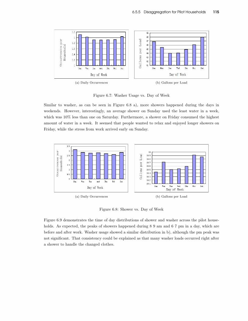
6.5.5 Disaggregation for Pilot Households 115
(a) Daily Occurrences (b) Gallons per Load
Figure 6.7: Washer Usage vs. Day of Week
Similar to washer, as can be seen in Figure 6.8 a), more showers happened during the days in
weekends. However, interestingly, an average shower on Sunday used the least water in a week,
which was 10% less than one on Saturday. Furthermore, a shower on Friday consumed the highest
amount of water in a week. It seemed that people wanted to relax and enjoyed longer showers on
Friday, while the stress from work arrived early on Sunday.
(a) Daily Occurrences (b) Gallons per Load
Figure 6.8: Shower vs. Day of Week
Figure 6.9 demonstrates the time of day distributions of shower and washer across the pilot house-
holds. As expected, the peaks of showers happened during 8 9 am and 6 7 pm in a day, which are
before and after work. Washer usage showed a similar distribution in b), although the pm peak was
not significant. That consistency could be explained as that many washer loads occurred right after
a shower to handle the changed clothes.

6.6 Related Work 116
(a) Shower (b) Washer Usage
Figure 6.9: Shower/Washer vs. Time of Day
6.6 Related Work
Non-intrusive load monitoring has been proposed based on analyzing steady state change and tran-
sient state change. So far most of the research effort has been focused on electricity load disaggrega-
tion with high sample rate [246,279,215,273,284,213,216]. A power meter with high sample rate (¿=
1Hz) can identify most of the state changes of multiple metrics (e.g., power, reactive power, voltage,
and harmonics) caused by individual appliances in a real-world home. Based on state change of cur-
rent and voltage, a non-intrusive load monitoring approach [246] was proposed to determine power
consumption of individual appliances. An electrical noise sensor has been used to disaggregate con-
sumption by running SVM on transient noise of turning on and off appliances [279]. By measuring
voltage of each outlet in a house, one approach [213] applied kNN and SVM to classify appliances.
This approach collected peak, average, and RMS of voltage of a single target with 4kHz sample rate,
and achieved best results using an NN classifier. An NN-based disaggregation approach has been
proposed to identify appliances with 90% accuracy using only the main power meter [215,216]. The
features it used consist of power, reactive power, voltage RMS, and harmonics for state transition.
RECAP has recently been proposed using artificial neural network (ANN) to disaggregate electricity
usage [284]. Features including power factor, peak and RMS of voltage and current were aggregated
every minute and analyzed in a 3-layer ANN. To extract better features, Matrix Pencil [273] has
been proposed to model each signal as complex plan, and use residues and poles as features for
disaggregation. Improved disaggregation results have been demonstrated.
Compared with electricity disaggregation, residential water disaggregation has attracted much less
research effort. To the best of our knowledge, there has not been any design that can disaggregate
water consumption either using a single water meter or from a sample rate lower than 500Hz.
Microphone-based sensors were applied on major water pipes (cold inlet, hot inlet, and sewing) to
recognize usage activities [237]. Combining the timestamps that these microphones detect noise, the
authors identified most of the water usages. However, this approach has difficulties to disaggregate
concurrent activities and cannot determine water volume. Integration of a water meter and a

6.6 Related Work 117
network of accelerometers [261] has been proposed to estimate the flow rates based on pipe vibration.
This approach has been applied in laboratory environments to disaggregate water usage. To avoid
accessing water pipes, an approach using pressure sensor on main source [238] was proposed to
identify fixtures. This approach applies hierarchical classifiers to first detect valve open and close
events, and then label fixtures. Due to the 1 kHz sample rate, it can clearly capture on and off
signals of fixtures from water pressure.

Chapter 7 118
Chapter 7
Application 2:Wireless PassiveDevice Fingerprintingusing Infinite HiddenMarkov Random Field
This chapter presents a new concept of device fingerprinting (or profiling) to enhance wireless se-
curity using Infinite Hidden Markov Random Field (iHMRF). Wireless device fingerprinting is an
emerging approach for detecting spoofing attacks in wireless network. Existing methods utilize ei-
ther time-independent features or time-dependent features, but not both concurrently due to the
complexity of different dynamic patterns. In this paper, we present a unified approach to finger-
printing based on iHMRF. The proposed approach is able to model both time-independent and
time-dependent features, and to automatically detect the number of devices that is dynamically
varying. We propose the first iHMRF-based online classification algorithm for wireless environment
using variational incremental inference, micro-clustering techniques, and batch updates. Extensive
simulation evaluations demonstrate the effectiveness and efficiency of this new approach.
The rest of the chapter is organized as follows. Section 7.1 introduces the background of the
problem. Section 7.2 formalizes the fingerprinting problem based on both time-dependent and
time-independent features. Section 7.3 discusses theoretical preliminaries, including Hidden Markov
Random Field (HMRF) and infinite Gaussian Mixture Model (iGMM). Section 7.4 formulates an
infinite hidden Markov random field (iHMRF) model for the fingerprinting problem, and Section 7.5
presents a new incremental inference algorithm for wireless streaming environment. Empirical vali-
dations of our proposed fingerprinting framework are presented in Section 7.6. The paper concludes
and discusses our future work in Section 7.7.

7.1 Introduction 119
7.1 Introduction
Nowadays, the proliferation of mobile devices moves the wireless networks toward “anytime-anywhere”
mobile service model. However, the open nature of wireless networks renders them susceptible to
various types of spoofing attacks. For example, the adversaries can collect nodes’ identity infor-
mation by passively monitoring the network traffic, and then masquerade as legitimate nodes to
disrupt network operations. Various attacks can be launched, such as packet injection [242], Sybil
attack [231], masquerade attack [235], etc. These identify-based attacks may hinder normal com-
munication and result in privacy leakage, which will lead to a huge outbreak of cybercrimes. As a
result, how to detect the presence of identity spoofing becomes a critical issue.
Two categories of existing solutions exist to detect identity spoofing attacks, namely, active detection
and passive detection. Active detection allows additional messages to be injected into the network,
such as challenges and responses used in cryptographic-based schemes for user authentication. In
the case that the entire node being compromised such that the cryptographic keys are exposed,
location related information can be used to facilitate node authentication. For example, in [71],
specific chipset, firmware or the driver of an 802.11 wireless device can be identified by watching
its responses to a crafted malformed 802.11 frames. However, the downside of active detection
methods lies in its requirement on extra message exchanges, which will accelerate the energy usage
and consume available bandwidth. In addition, the responses can also be spoofed, if they are device
dependent.
In contrast, passive detection methods extract device specific features from message transmissions,
which can be categorized as time-independent and time-dependent features. The main strength is
that these features are device dependent and hence can be used as an unique pattern to fingerprint
a specific device. Particularly, time-independent features include clock skew (observed from message
time stamps), sequence number anomalies (in MAC frames), timing (of probe frames for channel
scanning), and various RF parameters (transient phases at the onset of transmissions, frequency
offsets, phase offsets, I/Q offsets, etc.) [275]. Time-dependent features include radio signal strength
(RSS), angle of arrival, time of arrival, differential received signal strength, frequency difference
of arrival, etc. Note that, time-independent features refer to the signal measurements that have
constant mean values and are only randomized by white noises across the time. Time-dependent
features refer to the signal measurements whose mean values are time varying due to the essential
dynamical nature.
For the fingerprinting methods based on time-independent features [73,275,235,287,225,297], though
with a variety of implementations, basically it is assumed that the features form a cluster for each
device, which can be regarded as the unique fingerprinting pattern to identify the device. Two most
recent works are conducted by Brik et al. [73] and Nguyen et al. [275]. Brik et al. [73] proposed
the Passive RAdio-metric Device Identification System (PARADIS) utilizing modulation domain
radio-metrics, such as carrier frequency error, I/Q offset, etc. Nguyen et al. [275] further proposed
an unsupervised clustering method based on non-parametric Bayesian method and infinite Gaus-

7.1 Introduction 120
sian mixture model, which can automatically determine the number of clusters. To summarize,
time-independent features can be regarded as accurate and robust wireless signatures for particular
devices. However, the fingerprinting methods using time-independent features also have some limita-
tions. For example, these features are much harder to extract. Usually, some high-end measurement
devices are required to perform feature extraction. Moreover, the accuracy of these feature relies on
the precision of the measurement devices. Therefore, although time-dependent features are accurate
wireless signatures, the extracted features might include some errors due to the limitation of wireless
measurements.
For time-dependent features, the most popular family of methods for device identification is RSS-
based. In [72], a geographic location based identification technique against masquerading threats
was employed, where two alternate approaches are proposed: distance ratio test (DRT), which uti-
lizes the received signal strength (RSS) of a device, and distance difference test (DDT), which relies
on the received signal’s relative phase difference when the signal is received at different devices.
Zhao et al. [70] proposed a radio environment map (REM) which is a comprehensive database of
geographical features, available services, spectral regulations, locations, and activities of radio de-
vices and policies. Identification of cognitive radio (CR) node through an analysis of the transmitted
signal is investigated in [69] where wavelet transform is utilized to identify the transmitter finger-
print. However, the RSS measurements are time varying and only provide coarse spatial resolution.
Therefore, due to the dynamic nature, time-dependent features, such as RSS, cannot be regarded
as an accurate and reliable wireless signature alone.
The goal of this paper is to improve existing detection methods by considering additional features
that could potentially help improve the fingerprinting performance. Studies have been shown that
both time-independent features (e.g., frequency difference and phase shift difference) and time-
dependent features (e.g., RSS and time difference of arrival) can be used to do spoofing detection
[73, 235, 275, 287, 225, 297, 296, 298]. In this paper, we propose to concurrently model all the useful
features in a unified statistical framework, based on infinite hidden Markov random field (iHMRF).
All the device dependent features can be categorized into time-independent and time-dependent
features. The autocorrelation on time-dependent features is captured by using the so-called Markov
Property in iHMRF, in which data points that are similar on time-dependent features tend to have
consistent cluster labels. The time-independent features are captured through embedded Gaussian
mxitures in iHMRF. The main contributions of this work can be summarized as follows:
1. Design of a unified fingerprinting framework. To the best of our knowledge, this is the
first statistical approach to model both time-dependent and time-independent features in a
systematic framework for device fingerprinting.
2. Formulation of the fingerprinting problem via iHMRF modeling. We propose a novel
application of the iHMRF model to the device fingerprinting problem that captures correlations
on time-dependent features using the Markov property, and correlations on time-independent
features using an embedded Gaussian mixture model.

7.2 Related Work 121
3. Design of an online learning algorithm. We propose a new online classification algorithm
for the fingerprinting problem based on variational incremental inference, micro-clustering
techniques, and batch updates.
4. Comprehensive empirical validations. We conducted extensive simulations on a variety
of scenarios to validate the effectiveness and efficiency of our proposed techniques, competing
with existing state-of-the-art methods.
7.2 Related Work
A large body of literature has been dedicated to the issue of wireless device identification for detecting
spoofing attacks. In this section, we review the most relevant work in the literature. Based on
different types of features utilized, we classify these methods into two categories, including radio-
metric based methods, and radio signal strength (RSS) based methods.
7.2.1 Radio-metric Based Device Fingerprinting
In [73], Brik et al. proposed the Passive RAdio-metric Device Identification System (PARADIS)
utilizing modulation domain radio-metrics, such as carrier frequency error, I/Q offset, etc. The
experimental results show that these device dependent radio-metrics can effectively differentiate
devices. However, this method requires a training phase to collect the fingerprints of legitimate
nodes. Nguyen et al. [275] further proposed an unsupervised clustering method based on non-
parametric Bayesian method and infinite Gaussian mixture model. Without knowing the number of
devices, this method can automatically identify different devices by clustering their emitted packets
into different clusters. Our method also builds upon a non-parametric Bayesian framework for
unsupervised clustering. However, our method not only considers device dependent radio-metrics,
but also takes other device independent features into consideration to greatly improve the device
identification performance.
7.2.2 RSS Based Device Fingerprinting
Compared with radio-metric features, RSS feature is much easier to obtain, which makes RSS a
popular feature for device fingerprinting. Faria et al. [235] demonstrated strong correlations between
RSS signals and the physical location of devices, and proposed to use signalprint, a vector of RSS
values measured by surrounding Access Points (APs), to identify wireless devices for detecting
spoofing attacks. Sheng et al. [287] extended [235] and applied Gaussian mixture model to identify
clusters of the RSS readings. Chen et al. [225] used RSS and K-means cluster analysis. In both [287]
and [225], the number of clusters needs to be predefined. Later, Yang et al. [297] proposed two
cluster-based mechanisms that can automatically determine cluster numbers.

7.3 Features for Device Fingerprinting 122
However, the aforementioned methods [235, 287, 225, 297] only work in a static network (e.g., each
device is fixed in a specific location) and may raise a large number of false alarms in a mobile
network. The RSS profiles may change over time due to the nature of wireless device mobility. To
capture the RSS time-dependent property, Yang et al. [296] proposed the DEMOTE system that
partition the RSS trace of a node identity into two separate RSS traces, in which one trace is related
to a genuine node, and the other is related to a potential attacker. If the correlation between the
two traces is lower than a threshold, an alarm is alerted. They focused on two-class situations where
one genuine node and one attacker share a single identity (e.g., MAC address). This solution may
not be applicable to situations with multiple attackers sharing the same identity. Zeng et al. [298]
proposed a reciprocal channel variation-based identification (RCVI) technique to detect spoofing
attacks in mobile wireless networks. RCVI applies location de-correlation and reciprocal channel
variation to detect the original devices of all packets. However, this method assumes a bidirectional
communication between the genuine and the victim nodes. Therefore, it is not a completely passive
detection and requires senders to send the RSS information, which may cause unnecessary network
overheads.
Our paper also focuses on dynamic mobile networks. We observe that the above RSS based solution
for mobile networks share two more limitations. First, they both assume implicitly that wireless
devices and access points (AP) communicate periodically, and hence high sample rate location
features (e.g., RSS, TDOA) could be extracted. Second, they both consider device identification
(e.g., MAC address) into their fingerprinting process. The use of forgeable user identity information
may make the methods vulnerable to advanced spoofing attacks. For example, an attacker may
inject packets with randomly assigned device MAC addresses into the wireless network. This attack
will be hard to be detected if these MAC-addresses related victim devices are evaluated separately.
In contrary, our method takes the low sampling rate case into consideration. In addition, we neglect
the forgeable user identity information in our fingerprinting framework.
7.3 Features for Device Fingerprinting
Device fingerprinting means utilizing a set of unique features of devices that when exploited can be
used to differentiate wireless devices. Fingerprinting features can be classified in several ways. For
example, it can be categorize as time-dependent or time-independent features. As the name says
that some of the features varies over the time, whereas the others remain unchanged. There can be
device dependent and device-independent features as well. There can be transmitter fingerprinting
and receiver fingerprinting. The transmitter fingerprints are different than receiver’s radio-metric
parameters’ such as received power and are unique to the transmitter and not altered by the channel
condition and receiver structure.
In this section we briefly discuss about notable features that can be exploited for iHMRF based device
fingerprinting. Typically some common features of signal measurements/classifications are: angle-
of-arrival (AOA), received signal strength (RSS), time-of-arrival (TOA) and frequency-of-arrival

7.3.1 Time Measurement 123
(FOA). However, sometimes difference measurement features are well suited for creating traces for
particular applications. For example, time-difference-of-arrival (TDOA), frequency-difference-of-
arrival (FDOA), differential received signal strength (DRSS), phase shift difference (PSD) etc.
7.3.1 Time Measurement
The time required for a signal to travel from the transmitter (client or node) to the receiver (anchor or
access point) is directly proportional to the distance between them. The time-of-arrival (TOA) and
time-difference-of-arrival (TDOA) follows this principle. Propagation time measurement requires
synchronization between transmitter and receiver and knowledge of transmission and reception times
at one position. On the other hand, time difference measurements eliminates need for node to be
synchronized to anchors, but requires synchronization between anchors and doesn’t directly give
the distance between transmitter and receiver. The trilateration, conversion of the observations
to distances, from TOA or TDOA is done by d = cτ , where d is the distance, τ is the observed
time of flight (transmit time - receive time), and c is the propagation speed. The distance (from
observations) related to positions
dm = |(x, y) − (xm, ym)|2 ,m = 1, 2, 3, (7.1)
where (x, y) is the client position, (x1, y1), (x2, y2), and (x3, y3) are anchor positions, and |(x, y)|2 =√
x2 + y2. Here we have three non-linear equations with two unknowns, and it can be shown that
there is a single solution. Solving the equations requires more advanced algorithm unless linearization
technique applied. Using two observation points, TDOA can be calculated by
d = d1 − d2 = |(x, y) − (x1, y1)|2 − |(x, y) − (x2, y2)|2 .
The key sources of time measurement errors are: 1) synchronization error due imperfect reference
clock, measurement error such as error to determine the exact time of arrival of the signal and
signal fading (i.e., multipath), and environmental errors (e.g., non-line-of-sight propagation) that
adds delay not related to distance.
7.3.2 Frequency Measurement
Measuring ∆f , the difference between the carrier frequency of the received signal and the one of the
transmitted signal, can provide estimation about the device’s whereabout. The frequency difference
is a strong feature since each wireless transmitter has its own oscillator, and each oscillator creates
a unique carrier frequency. Frequency shift of the received signal is related to the velocity vector of
the transmitter relative to the receiver. Note that this mobility of transmitter introduces Doppler
Effect in the signal that smears signal frequency that can be measured. Frequency difference are

7.3.3 Phase Shift Difference Measurement 124
Device 1 Device 2
Figure 7.1: Illustration of phase shift difference for constellation of QPSK symbols of twotransmitters
more commonly used and obtained from Cross Ambiguity Function
C (∆f,∆t) =
∫ T
0
x (t)x∗ (t+ ∆t) e−jπ∆ftdt. (7.2)
It differs from time dependent features in that the frequency/phase shift feature observation points
must be in relative motion with respect to each other and the source, and FDOA can be calculated
by
f = f1 − f2 =v1λ
cos θ1 −v2λ
cos θ2. (7.3)
A major drawback of this measurement feature is that large amounts of data must be moved between
observation points or to a central position to do the cross-correlation that is necessary to estimate the
frequency shift. Other common source of frequency measurement errors are: 1) imperfect frequency
reference, 2) measurement errors such as noise, multipath etc., and non-stationary nature of the
frequency.
7.3.3 Phase Shift Difference Measurement
On top of aforementioned method, one can differentiate devices by looking into device’s I-Q phase
characteristic. Ideally the phase shift from one constellation to a neighbor one is 180 for BPSK
modulation and 90 for QPSK modulation. I-Q phase characteristics are different for I-phase and
Q-phase. The constellation may deviate from original position due to hardware variability, and
different devices have different constellations. Therefore, this feature can be measured and used as
classifier as well. Figure 7.1 shows an illustrative example of device signal constellations.
In this example we used QPSK as modulation of choice and considered feature extracted from the
constellation of QPSK. In QPSK, four symbols with different phases are transmitted where each
symbol represents two bits. Mathematically the transmitted symbol can be represented as
si (t) =
√
2Es
Tcos(
2πfct+ (2n− 1)π
4
)
, (7.4)

7.3.4 Angle of Arrival Measurement 125
where Es is the transmission power, T is symbol period, fc is the carrier frequency, and n is the
index for the four possible constellations. By changing n, we can vary the phases of the signal,
creating four phases π4 , 3π
4 , 5π4 , and 7π
4 . In the ideal case, the phase shift from one symbol to its
neighbor is 90. However, the transmitter amplifiers for I-phase and Q-phase might be different.
Consequently, the degree shift can have some variances.
7.3.4 Angle of Arrival Measurement
The direction of the nodes (or clients or devices) relative to the access points (or anchor) is equal to
the observed received angle-of-arrival (AOA or DOA), that can be used to create trace of device by
calculating the position of the nodes, or determining the angle of the position of node relative to the
access point. This process is called ‘triangulation’ where a minimum of two anchors and reference
coordinate are needed and can be calculated by two linear equations
y = tan θ1x+ (y1 − tan θ1x1) ,
y = tan θ2x+ (y2 − tan θ2x2) , (7.5)
where θ are angle between device and anchor and (x1, y1) and (x2, y2) are locations of the two
anchors.
Features Time Independent Time Dependent
Device DependentFrequency-of-arrival (FOA) Radio Signal Strength (RSS)
I/Q Offset Signal Noise Ratio (SNR)
Device Independent
Time-Difference-Of-Arrival (TDOA)
Phase Shift Difference (FSD) Time-Of-Arrival (TOA)
Carrier Frequency Offset (CFO) Angle-Of-Arrival (AOA)
Frequency-Difference-Of-Arrival (FDOA)
Table 7.1: Device Fingerprinting Features
Possible source of AOA errors are reference error (what is east?), measurement error for thermal
noise, environmental error (non-line-of-sight propagation).
7.3.5 Radio Signal Strength (RSS) Measurement
In free space signal power decays exponentially with distance that can be roughly estimated by
received signal strength. Translation of RSS measurement to distance requires knowledge of the
transmit power (i.e., reference value) and Knowledge of the relationship between distance and power

7.3.5 Radio Signal Strength (RSS) Measurement 126
decay (propagation model)
Pr (d) = P0 + 10n log10
(
d
d0
)
+Xσ, (7.6)
where P0 is the received power at reference distance d0 and Pr is the observed received power, d is
the distances, and n is the path loss exponent. The trilateration from RSS is done in the same way
as time measurement, except the conversion of the observations to distances is done by
d0 = d10
(
P0−Pr10n
)
. (7.7)
Differential RSS measurements eliminate need for transmit power knowledge and can provide im-
proved performance in correlated shadowing. The key limitations of this feature are: 1) Imperfect
knowledge of the transmit power or antenna gain, 2) measurement error such as signal fading (i.e.,
multipath), interference, and thermal noise, and 3) Environmental errors (e.g., non-line-of-sight
propagation) such as shadowing, biases the resulting distance estimate, and Imperfect knowledge of
the propagation exponent (model error).
Interestingly, the channel gain can be used as trait as well. The amplitude of received signal is
proportional to the channel gain, Ap. The general consensus is that the signals transmitted from the
same device over a short duration tend to have similar amplitude or effect of channel, even though
the absolute value of the amplitude is generally unknown. If the channel is Rayleigh faded multipath
channel, the channel gain can be expressed as
Ap∼= d−β |h|, (7.8)
where |h| is the fading component that is normally distributed with N (0, σ2h), d is distance from a
transmitted device to the sensing device, β is the path loss exponent. Thus the received signal gain
Ap can be described by the distribution
Ap ∼ N (0, d−2βσ2h). (7.9)
A notable difference is that by looking into channel characteristics only does not infer the locations
of devices directly, rather Ap as one more feature for the identification.
The aforementioned features are generic to most radio technologies. There are few other features
that can be used for specific technologies. For example, second-order cyclostationary feature of
OFDM signal can be used for identification.

7.4 Problem Formulation 127
7.4 Problem Formulation
Suppose we are given a sequence of N packet feature vectors (x1, s1, t1), · · · , (xN , sN , tN), where
xi ∈ Rp, si ∈ Rd, p and d refer to the numbers of time-independent and time-dependent features,
respectively, and ti refers to the arrival time of the ith packet on an access point. The goal is to
identity the sequence of hidden states (device labels): z1, · · · , zN , where zi ∈ 1, 2, · · · , C refers
to the hidden state of the packet feature vector (xi, si, ti), and C refers to the total number of
hidden states. There may exist some tis, in which the time distance between ti and ti+1 is large,
and the dependence between si and si+1 may be highly degraded because of the low collection rate.
The number C of hidden states is unknown and will be estimated using nonparametric Bayesian
techniques.
Figure 7.2: Features extraction from packets
The process of feature extraction is shown in Figure 1. Suppose multiple access points (APs) are
deployed across the network environment, which collect and send traffic information to a centralized
server, called a wireless appliance (WA). Each AP reports the RSS measurement for each packet
received, as well as other device dependent features, such as frequency difference and phase shift
difference. WA receives all the information and creates a fingerprint feature vector for each packet.
Note that, there may be some duplicated features reported by APs, such as frequency differences of
the repeated packets received by different APs. We will randomly select and keep one version, since
for device dependent features all different versions should exhibit similar patterns.
Several assumptions and constraints are stated as follows:
1. There is no training data about the fingerprints of legitimate devices available. The problem
will be addressed in a completely unsupervised manner.
2. The collection rate of RSS measurements may be unstable. Sometimes the collection rate will
be low, e.g., some devices are in standby status and there are no communications between the
devices and access points. Sometimes the collection rate will be high, e.g., the device users are
using calling services, sending text messages, or serving internet.

7.5 Theoretical Backgrounds 128
3. The number of clients (devices) is unknown and dynamic. Current clients may leave the
network and new clients may join the network in any time.
4. A wireless network may have a large number of concurrent clients. We will need to evaluate
the impact of the number of concurrent clients on the fingerprinting performance.
5. It is not allowed to add any additional out-band message exchanges. The problem will be
addressed using passive detection strategies.
6. Attackers have the ability to adjust transmission powers to increase localization uncertainties.
7. Attackers have the ability to masquerade as a large number of clients. Hence, we will not trust
device identity information and only consider device dependent features for fingerprinting.
7.5 Theoretical Backgrounds
This section introduces two basic statistical models, including Hidden Markov Random Field (HMRF)
and infinite Gaussian Mixture Model (iGMM). These two models provide theoretical fundamentals
to Infinite Hidden Markov Random Field (iHMRF) that will be applied to do wireless device finger-
printing.
7.5.1 Hidden Markov Random Field
Suppose we have a set of observations (x1, s1), · · · , (xN , sN ), where each observation (xi, si) has
p features (xi ∈ Rp) and d spatial coordinates (si ∈ Rd). Denote X = x1, · · · ,xN and S =
s1, · · · , sN. The objective is to infer the latent variables Z = z1, · · · , zn based on X and S,
where zi ∈ C, and C = 1, · · · , C denotes the set of class labels.
Hidden Markov Random Field (HMRF) can be described as a two-layer hierarchical model, including
the latent layer Z and the observation layer X. For the latent layer Z, HMRF considers spatial
dependencies between the observations Z. Nearby variables will have higher correlations than distant
variables. The neighborhood relationship is decided based on their closeness on spatial coordinates
s1, · · · , sn, such as by the K-nearest neighbors rule. This so-called Markov property can be
formulated as
p(zi = c|N(zi); γ) =1
Z(γ)exp
(
−∑
c∈Ci
Vc(zi = c,N(zi)|β)
)
, (7.10)
where Z(β) refers to a normalization constant, β is called the inverse temperature of the model,
N(zi) refers to the neighbors of zi, and Ci refers to the set of cliques, each of which contains zi as a
member. A clique c is defined as any set of variables such that all the variables in c are neighbors
to each other. Vc(·) is called clique potential, which is a measure of the consistence of the variables

7.5.2 Infinite Gaussian Mixture Model 129
in c. A clique potential Vc(Z|β) can be defined as
Vc(Z|γ) = β∏
i,j∈c
δ(zi − zj). (7.11)
The joint distribution p(Z|β) of an HMRF model is
p(Z) =∏
i
p(zi|N(zi); γ) =1
Z(γ)exp
(
−∑
c∈CVc(Z|β)
)
, (7.12)
where Z(β) is a normalization constant.
For the observation layer, HMRF defines the conditional distribution p(X|Z) as
p(X|Z; Θ) =
N∏
i=1
p(xi|zi; Θzi), (7.13)
p(xi|zi; Θzi) = N (xi|µzi
,Σzi), (7.14)
where each observation xi follows a Gaussian distribution conditioned on the latent variable zi.
Each class is related to a distinct Gaussian distribution, and we have totally C Gaussian mixtures.
Denote the parameters Θ = ΘcCc=1, and Θc = µc,Σc.
7.5.2 Infinite Gaussian Mixture Model
Infinite Gaussian Mixture Model (iGMM), also named Dirichlet Process Gaussian Mixture Model
(DPGMM), is an extension of the traditional Gaussian Mixture Model (GMM) to support an finite
number of Gaussian mixtures. Denote X = x1, · · · ,xN as observations, and Z = z1, · · · , zN as
latent class labels, where zi ∈ Ci = 1, · · · , C. Note that, different from HMRF, spatial coordinates
(attributes) are not considered here. iGMM can be defined as
vc|α ∼ Beta(1, α), c = 1, · · · ,∞, (7.15)
Θc|G0 ∼ G0, c = 1, · · · ,∞, (7.16)
xi|zi = c; Θc ∼ N (µc,Σc), (7.17)
zi|π(v) ∼ Multi(π(v)), (7.18)
where πc(v) = vc
∏c−1i=1 (1− vi). To interpret this model, we can look at its data generating process:
1. Draw vc|α ∼ Beta(1, α), c = 1, 2, · · · ,
2. Draw Θc = µc,Σc|G0 ∼ G0, c = 1, 2, · · · ,
3. For the ith data point
(a) Draw zi|v1, v2, · · · ∼Multi(π(v)),

7.6 Infinite Hidden Markov Random Field (iHMRF) 130
(b) Draw xi|zi = c ∼ N (, µc,Σc).
Particularly, step 1 samples a countably infinite set of random variables v from a beta distribution
Beta(1, α), where α is a hyper-parameter. The prior probabilities π(v) can then be calculated as
πc(v) = vc
c−1∏
i=1
(1 − vi), c = 1, 2, · · ·. (7.19)
Step 2 samples the model parameters Θc for each mixture c from a base distribution G0, which is
defined as
Σc ∼ InverseWishartυ0(Λ0), (7.20)
µc ∼ N (µ0,Σc/K0), (7.21)
where υ, µ0,Λ0 are the hyper-parameters. Steps 1 and 2 are called the stick-breaking construction
of a dirichlet process (DP). Given the prior probabilities π(v) and the Gaussian distribution param-
eters Θ1,Θ2, · · · , the last step (Step 3) is to i.i.d. sample N observations xi, zi, i = 1, 2, · · · , N .
For each point i, step 3.1 samples its class label from Multi(π(v)), and step 3.2 samples its features
xi from the corresponding Gaussian distribution N (µc,Σc).
Figure 7.3: Graphical Model Representation of iGMM
7.6 Infinite Hidden Markov Random Field (iHMRF)
Given the data set X = x1, · · · ,xN, S = s1, · · · , sN, and T = t1, t2, · · · , tN, with the unknown
class labels Z = z1, · · · , zN. The iHMRF model can be represented by a graphical model as shown
in Figure 7.4. Each node represents a random variable (or vector), and each dot represents a hyper-
parameter. The filled nodes refer to observations and blank nodes refer to latent variables. Basically,
we first use spatio-temporal features (s1, t1), · · · , (sN , tN ) to build a neighborhood graph for the

7.6 Infinite Hidden Markov Random Field (iHMRF) 131
latent state variables z1, · · · , zN, in which states zi and zj are connected by an undirected edge
if they are spatial temporal neighbors. Each latent state variable zi will emit an observation xi.
The iHMRF model is designed by this manner. According to the key property of a hidden Markov
random field, the hidden states should be consistent if they are neighbors to each other. However,
two neighbor nodes zi and zj could be assigned different cluster labels if their emission observations
xi and xj belong to two different Gaussian distributions. The iHMRF model can be defined as
follows:
Definition 1 Infinite Hidden Markov Random Field (iHMRF)
α|λ1, λ2 ∼ Gamma(λ1, λ2) (7.22)
βc|α ∼ Beta(1, α), c = 1, · · · ,∞, (7.23)
Θc|G0 ∼ G0, c = 1, · · · ,∞, (7.24)
xi|zi = c; Θc ∼ N (µc,Σc), (7.25)
zi|π(β) ∼ Multi(π(β)), (7.26)
p(Z) =
N∏
i=1
p(zi|π(β), zi,N(zi)), (7.27)
p(zi|π(β), zi,N(zi)) = p(zi = c|π(β))
×p(zi = c|zi,N(zi); γ), (7.28)
where Θc|G0 stands for:
Σc ∼ InverseWishartυ0(Λ0), (7.29)
µc ∼ N (g0,Σc/η0), (7.30)
and
p(zi = c|N(zi); γ) =1
Z(γ)exp
(
−∑
c∈Ci
Vc(zi = c,N(zi); γ)
)
, (7.31)
where λ1, λ2, γ, υ0,g0,Λ0, η0 are hyper-parameters.
Compared with HMRF and iGMM, the iHMRF model has three major advantages: First, iHMRF
is able to capture Gaussian mixtures information and spatial dependencies between latent variables
ziNi=1 concurrently, through Equations (7.25) and (7.28). As a result, iHMRF tends to decide the
value of zi both based on its neighbors and its closest Gaussian mixture. When conflicts occur, that
means the class labels of its spatial neighbors are not consistent with its closest Gaussian mixture, we
can adjust the inverse temperature parameter γ to decide the weight we put on each side. A smaller
value of γ implies that the model will favor more on the Gaussian mixtures information. In the
extreme when γ = 0, the model will degenerate and become equivalent to iGMM. Second, iHMRF is
able to automatically estimate the number of class labels (clusters), since Dirichlet Process (DP) is
used as the prior distribution for zi and xi. Third, iHMRF is robust to transmission power changes.

7.7 Incremental Variational Inference for the IHMRF Model 132
Figure 7.4: Graphical Model Representation of iHMRF
When a device changes its transmission power, it tends to increase the spatial entropy and makes
its spatial trajectory more highlighted than those of other devices. We observe that iHMRF inherits
the advantages of both HMRF and iGMM.
Based on the above iHMRF model specification, the fingerprinting problem can be reformulated as
a maximum-a-posterior (MAP) problem. It is to estimate the latent variables z1, · · · , zN, such
that their joint posterior probability based on the observations x1, · · · ,xN can be maximized:
z1, · · · , zN = argminz1,··· ,zN
p(z1, · · · , zN |x1, · · · ,xN ). (7.32)
Because the wireless device environment under study is a streaming environment, it is more ap-
propriate to do incremental inference (or classification). We will introduce efficient incremental
techniques in the next section 7.7.
7.7 Incremental Variational Inference for the IHMRF Model
Inference for the iHMRF model can be conducted based on variational inference, Markov chain
Monte Carlo (MCMC), and other methods. In this paper, we are focused on variational inference,
because it is computationally more scalable than MCMC techniques, and hence more applicable to
wireless streaming environment. Denote Φ = Z,Θ,v as the set of all latent random variables,
and θ = γ, λ1, λ2, υ0,g0,Λ0 as the set of hyper-parameters. The objective is to infer the latent Φ
given the observations X and hyper-parameters θ. Because it is intractable to calculate the posterior
p(Φ|X, θ), variance inference is applied to approximate the posterior with a parametric family of

7.7 Incremental Variational Inference for the IHMRF Model 133
factorized distributions q(Φ|X, θ) of the form
q(Φ|X, θ) = q(Z)q(α;λ1, λ2)
C−1∏
c=1
q(βc; ζc,1, ζc,2)
×C∏
c=1
q(µc,Σc; υc, ηc, gc, Λc). (7.33)
Denote the variational Free Energy functional as
F (q;X, θ) =
∫
q(Φ; θ) logp(Φ|X, θ)
q(Φ; θ)dΦ, (7.34)
which is a lower bound of the original log-evidence ln p(X|θ). The optimal solution based on the
parametric family can be obtained by maximizing the Free Energy functional:
minimizeθ
F (q(θ);X, θ), (7.35)
where the variational parameters to be estimated include θ = λ1, λ2, ζc,1, ζc,2, υc, ηc,gc,Λc, Cc=1.
These parameters can be optimized iteratively by coordinate accent until convergence to a local
optimum. The results have been derived by Chatzis et.al. [223].
In this section, we will focus on incremental inference, instead of the above offline inference (7.35).
Incremental inference is more suitable for a streaming environment as existing in our device fin-
gerprinting problem. Assume that we have a buffer bucket with a limited size (e.g., N) to store
the streaming observations. When the bucket is full, it will be processed and all the observations
in the bucket will be classified. Then the bucket is cleaned and is ready to accept new incoming
observations. We may consider multiple buckets in the process line, such that when one bucket
is being processed, other buckets are ready to store new incoming observations. Denote a bucket
data as B(i) = (x(i)1 , s
(i)1 , t
(i)1 ), · · · , (x
(i)N , s
(i)N , t
(i)N ), where i refers to the bucket sequence number.
The incremental inference problem is to process the incoming buckets B(1),B(2), · · · incrementally.
We consider a similar strategy as used in iGMM [265, 243], and propose an incremental inference
framework for iHMRF. The key components are summarized as follows:
1. Compression Phase: When the observations have been classified to different clusters, each
cluster is separated into a number of microclusters that tend to have consistent cluster labels,
even when the clusters have been reformed due to the process of new bucket data. For each
microcluster, its sufficient statistics are stored and the data points inside are discarded to save
memory space and improve computational efficiency.
2. Model Building Phase: The incremental inference will be conducted based on microclusters,
instead of data points. Some microclusters are allowed to be isolated data points.
3. Incremental Batch Update Phase: The incremental model updates based on the new bucket
and previous buckets need not to start from scratch. The model information estimated based

7.7.1 Model Building Phase 134
on previous buckets will be considered to improve the incremental update efficiency.
The technical details of the above three components are discussed in Sections 7.7.1, 7.7.2, and 7.7.3,
respectively.
7.7.1 Model Building Phase
This phase assumes that the observations in the current buckets have already been grouped to a
set of microclusters. When this phase is first run (as the initialization step), each observation will
be regarded a microcluster. For later iterations, the microclusters are generated from the previous
iterations (see Section 7.7.2). Denote A as a specific microcluster, nA as the cluster size, and
xA = 1nA
∑
xi∈A xi. The model building phase is to solve the following constrained optimization
problem
minimizeq(Φ;θ)
∫
q(Φ; θ) logp(W |X ; θ)
q(Φ; θ)dΦ
subject to q(zi) = q(zj), if ∃A s.t. zi, zj ∈ A,
(7.36)
where q(Φ; θ) is a factorized parametric form as defined in 7.33. Notice the difference the above
problem (7.36) and the traditional offline problem (7.35). New constraints are defined such that the
data points in a same microcluster must have identical class labels. Because each microcluster is now
summarized by its sufficient statistics, the computational efficiency is greatly improved. The above
problem can be optimized iteratively by coordinate accent until convergence to a local optimum.
The solution for each iteration can be obtained as
ζc,1 = 1 +∑
A
nAq(A = c) (7.37)
ζc,2 = 〈α〉 +C∑
k=c+1
∑
A
nAq(A = k) (7.38)
wc =∑
A
nAq(A = c) (7.39)
xc =
∑
A nAq(A = c)xA
wc(7.40)
Ξ =∑
A
nAq(A = c)(xA − xc)(xA − xc)T (7.41)
q(A = c) ∝ p(A = c|(N)(A); γ)πc(β)p(xA|Θc), (7.42)
where N(A) refers to the neighbors of the micro-cluster A, which are defined similar to those based
on data points. Here, we use the spatial center point of a microcluster to represent its spatial
location, with sA = 1nA
∑
si∈A si, and use the center time to represent its time domain location, with
tA = 1nA
∑
ti∈A ti. Note that, only the solution components that are different from the traditional
offline solution are presented above. Readers are referred to [223] for the estimation of the other
model parameters that have the same result as the offline iHMRF model, including ζc, Λc, υc, ηc,
and gc.

7.7.2 Compression Phase 135
7.7.2 Compression Phase
This phase focuses on the generation of microclusters. The microclusters will be generated such
that the data points in each microcluster tend to be located in a same cluster, even when the overall
clusters have been reformed due to the process of new bucket data. To address this challenge, a
straightforward strategy is to generate multiple candidate clusters from different ways and then look
for the micoclusters, each of which never overlaps with more than one candidate cluster concurrently.
However, this strategy has two potential deficiencies: First, it is computationally expensive since the
number of different groups increases exponentially with the data size; Second, it does not consider
the behavior of future data points. An optimized strategy is to predict up to ∆ future points based
on the empirical distribution estimated from existing data (x1,x2, · · · ,xT ):
p(xT+1, · · · ,xT+∆) =
T+∆∏
i=T+1
1
T
T∑
t=1
δ(xi − xt). (7.43)
We define a modified Free Energy functional by taking expectation on ∆ unobserved future points
as
F (q;X, θ) =
∫
dxT+1, · · · , dxT+∆F (q;X, θ)
·p(xT+1, · · · ,xT+∆). (7.44)
The solution by maximizing the above modified Free Energy functional can be obtained as
ζc,1 = 1 + (1 +∆
T)∑
A
nAq(A = c) (7.45)
ζc,2 = 〈α〉 + (1 +∆
T)
C∑
k=c+1
∑
A
nAq(A = k) (7.46)
wc = (1 +∆
T)∑
A
nAq(A = c) (7.47)
xc = (1 +∆
T)
∑
A nAq(A = c)xA
wc(7.48)
Ξ = (1 +∆
T)∑
A
nAq(A = c)(xA − xc)
(xA − xc)T (7.49)
q(A = c) ∝ p(A = c|(N)(A); γ)πc(β)p(xA|Θc), (7.50)
To conduct the compression phase, we first apply the model building phase to generate clusters.
Then for each candidate cluster, we split it into two clusters along its principal component, and
refine the clusters based on the above update rules 7.45, until convergence. The gain on the free
energy function is denoted as ∆F (q;X, θ). The cluster with the largest ∆F (q;X, θ) will be selected
as the final splitting cluster. Iterate the process until convergence, e.g., the gain ∆F (q;X, θ) is

7.7.3 Incremental Batch Update Phase 136
smaller than a predefined threshold or the consumed memory is greater than the memory space
limit.
7.7.3 Incremental Batch Update Phase
This phase assumes that all previous bucket data have been processed, and we have obtained the
estimate variational parameters ηc,Λc, υc,gc, ζc,1:2, λ1:2, wc, xc,ΞcCc=1. Suppose a new bucket data
have been arrived, and it is necessary classify the new bucket data points and update all existing
clusters. Denote the new bucket data as (x(n)1 , s
(n)1 , t
(n)1 ), · · · , (x
(n)N , s
(n)N , t
(n)N ). The incremental
Batch update phase can be described as
ζc,1 = ζc,1 +
N∑
i=1
q(z(n)i = c) (7.51)
ζc,2 = ζc,2 +
C∑
k=c+1
N∑
i=1
q(z(n)i = k) (7.52)
wc = wc +
N∑
i=1
q(z(n)i = c) (7.53)
xc =xcwc +
∑Ni=1 q(z
(n)i = c)x
(n)i
wc(7.54)
Ξ = Ξ +
N∑
i=1
q(z(n)i = c)(x
(n)i − xc)
(x(n)i − xc)
T (7.55)
q(z(n)i = c) ∝ p(z
(n)i = c|N(zi))πc(β)p(x
(n)i |Θc). (7.56)
The basic idea is to apply Equation (7.56) to estimate q(z(n)i ), and apply Equations (7.51) to (7.55)
to update the variational parameters ζc,1:2, wc, xc, and Ξ. The other parameters that are consistent
with the offline iHMRF model are then updated by the equations derived in [223].
7.8 Simulation Result
This section presents an extensive simulation study to validate the effectiveness and efficiency of our
proposed techniques, compared with existing solutions, such as Gaussian Mixture Model (GMM) and
infinite Gaussian Mixture model (iGMM) [275]. For our fingerprinting framework, we studied the
performances of two inference algorithms, including the offline variational inference algorithm [223]
and our proposed online (incremental) inference algorithm.

7.8.1 Simulation Setup 137
7.8.1 Simulation Setup
The simulation data generator includes two components. The first component is the generation of
time-independent features. The same simulator design as used in [275] were applied to generate time-
independent features. Basically, a number of devices will be chosen randomly in an area of 40×40 in
the time-independent feature space, with variances of the clusters chosen random in the range from
0 to 1. We considered two time-independent features, such that the data can be easily visualized.
The second component is the generation of time dependent features. We considered RSS features
and assumed that the collected RSS features have been triangulated to three dimensional spatial
coordinates. This is appropriate for mobile devices, because for different time periods users may
travel to different spatial regions and different Access Points (AP) will be able to collect the related
RSS traces data. By converting the RSS features to spatial coordinates, we do not need to consider
the issue of missing values for different access points. We used UdelModels to generate mobile device
traces data, which is a widely used simulator for generating human trajectory data [260]. Changes
of transmission power were simulated by shifting a trace segment with a randomly selected distance
and direction.
We considered four major metrics to evaluate the effectiveness of our framework, including precision,
recall, F-measure, and rand index (IR). These metrics are defined based on true positive rate (TP),
false positive rate (FP), false native rate (FN), and true negative rate (TN), as interpreted in Table
7.2. These metrics are defined as Precision = TP/(TP + FP );Recall = TP/(TP + FN);F −
Measure = Precision×RecallPrecision+Recall ; and Rand− Index(RI) = TP+TN
TP+TN+FN+FP .
Table 7.2: Definition of TP, FP, FN, and TN
Same Cluster Different Clusters
Same Class TP FNDifferent Classes FP TN
We used UdelModels to generate four simulation datasets to cover a variety of scenarios, including
indoor and outdoor environments. The basic features of these data sets are summarized in the
following table 7.3. For each setting, we generated five different versions, in order to calculate the
uncertainty (standard deviation) of the classification performance.
Table 7.3: Simulation Data Settings
Description # of Penetrations (Peds) # of Cars
1 Building 10 Floors 5, 10, 15 5, 10, 15Real City (Chicago9B1k) 5, 10, 15 5, 10, 15
We compared our framework with two existing approaches, including GMM and iGMM. For our
framework, we employed two inference algorithms, including the offline variational inference algo-
rithm for iHMRF [223], abbreviated as iHMRF-VI, and our proposed incremental inference algo-
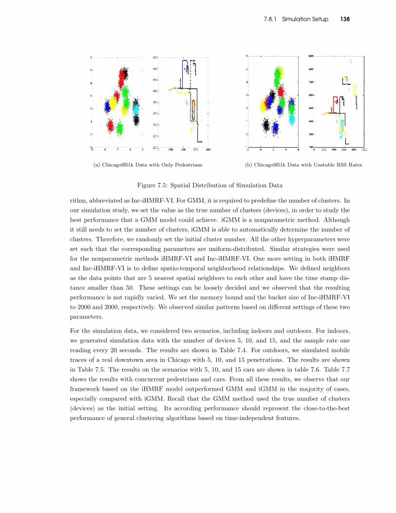
7.8.1 Simulation Setup 138
(a) Chicago9B1k Data with Only Pedestrians (b) Chicago9B1k Data with Unstable RSS Rates
Figure 7.5: Spatial Distribution of Simulation Data
rithm, abbreviated as Inc-iHMRF-VI. For GMM, it is required to predefine the number of clusters. In
our simulation study, we set the value as the true number of clusters (devices), in order to study the
best performance that a GMM model could achieve. iGMM is a nonparametric method. Although
it still needs to set the number of clusters, iGMM is able to automatically determine the number of
clusters. Therefore, we randomly set the initial cluster number. All the other hyperparameters were
set such that the corresponding parameters are uniform-distributed. Similar strategies were used
for the nonparametric methods iHMRF-VI and Inc-iHMRF-VI. One more setting in both iHMRF
and Inc-iHMRF-VI is to define spatio-temporal neighborhood relationships. We defined neighbors
as the data points that are 5 nearest spatial neighbors to each other and have the time stamp dis-
tance smaller than 50. These settings can be loosely decided and we observed that the resulting
performance is not rapidly varied. We set the memory bound and the bucket size of Inc-iHMRF-VI
to 2000 and 2000, respectively. We observed similar patterns based on different settings of these two
parameters.
For the simulation data, we considered two scenarios, including indoors and outdoors. For indoors,
we generated simulation data with the number of devices 5, 10, and 15, and the sample rate one
reading every 20 seconds. The results are shown in Table 7.4. For outdoors, we simulated mobile
traces of a real downtown area in Chicago with 5, 10, and 15 penetrations. The results are shown
in Table 7.5. The results on the scenarios with 5, 10, and 15 cars are shown in table 7.6. Table 7.7
shows the results with concurrent pedestrians and cars. From all these results, we observe that our
framework based on the iHMRF model outperformed GMM and iGMM in the majority of cases,
especially compared with iGMM. Recall that the GMM method used the true number of clusters
(devices) as the initial setting. Its according performance should represent the close-to-the-best
performance of general clustering algorithms based on time-independent features.

7.8.1 Simulation Setup 139
Table 7.4: Simulation Results Based on UdelModels with 1 Building 10 Floors
Methods # of Devices Precision Recall F-Measure Relative Index (RI)
iHMRF-VI 5 0.97 (0.02) 0.91 (0.13) 0.93 (0.07) 0.96 (0.04)10 0.72 (0.13) 0.81 (0.13) 0.76 (0.11) 0.93 (0.04)15 0.73 (0.09) 0.82 (0.06) 0.77 (0.07) 0.96 (0.01)
Inc-iHMRF-VI 5 0.88 (0.10) 0.94 (0.05) 0.91 (0.05) 0.95 (0.02)10 0.65 (0.28) 0.85 (0.14) 0.72 (0.23) 0.90 (0.09)15 0.51 (0.13) 0.79 (0.08) 0.62 (0.12) 0.92 (0.02)
iGMM-VI 5 0.86 (0.09) 0.44 (0.15) 0.57 (0.15) 0.80 (0.09)10 0.73 (0.11) 0.43 (0.10) 0.54 (0.10) 0.91 (0.03)15 0.56 (0.01) 0.30 (0.07) 0.38 (0.06) 0.92 (0.01)
GMM-EM 5 0.91 (0.15) 0.85 (0.22) 0.86 (0.16) 0.90 (0.10)10 0.72 (0.14) 0.83 (0.13) 0.77 (0.11) 0.93 (0.04)15 0.64 (0.11) 0.77 (0.06) 0.70 (0.08) 0.94 (0.01)
Table 7.5: Simulation Results Based on UdelModels - Chicago9Blk - with Pedestrians and Cars
Methods # of Devices Precision Recall F-Measure Relative Index (RI)
iHMRF-VI 5 Peds, 5 Cars 0.99 (0.01) 0.98 (0.01) 0.99 (0.01) 0.99 (0.01)10 Peds, 10 Cars 0.91 (0.10) 0.99 (0.10) 0.95 (0.05) 0.99 (0.01)15 Peds, 15 Cars 0.90 (0.09) 0.97 (0.02) 0.94 (0.05) 0.99 (0.01)
Inc-iHMRF-VI 5 Peds, 5 Cars 0.98 (0.02) 1.00 (0.00) 0.99 (0.01) 0.99 (0.01)10 Peds, 10 Cars 0.80 (0.13) 0.97 (0.04) 0.87 (0.08) 0.96 (0.02)15 Peds, 15 Cars 0.57 (0.07) 0.92 (0.08) 0.70 (0.07) 0.93 (0.02)
iGMM-VI 5 Peds, 5 Cars 0.90 (0.12) 0.29 (0.05) 0.44 (0.07) 0.80 (0.0610 Peds, 10 Cars 0.67 (0.08) 0.31 (0.06) 0.42 (0.06) 0.89 (0.02)15 Peds, 15 Cars 0.63 (0.06) 0.29 (0.06) 0.40 (0.06) 0.92 (0.01)
GMM-EM 5 Peds, 5 Cars 0.92 (0.13) 0.89 (0.06) 0.89 (0.07) 0.95 (0.03)10 Peds, 10 Cars 0.69 (0.08) 0.79 (0.11) 0.73 (0.09) 0.93 (0.03)15 Peds, 15 Cars 0.69 (0.12) 0.78 (0.06) 0.72 (0.08) 0.95 (0.02)
Table 7.6: Simulation Results Based on UdelModels - Chicago9Blk - with Only Cars
Methods # of Devices Precision Recall F-Measure Relative Index (RI)
iHMRF-VI 5 Cars 0.95 (0.03) 0.59 (0.08) 0.72 (0.06) 0.89 (0.02)10 Cars 0.83 (0.09) 0.55 (0.05) 0.66 (0.05) 0.93 (0.01)15 Cars 0.68 (0.08) 0.53 (0.09) 0.59 (0.08) 0.94 (0.01)
Inc-iHMRF-VI 5 Cars 0.89 (0.12) 0.98 (0.02) 0.93 (0.02) 0.97 (0.04)10 Cars 0.73 (0.11) 0.77 (0.09) 0.75 (0.06) 0.93 (0.02)15 Cars 0.56 (0.08) 0.83 (0.06) 0.66 (0.07) 0.93 (0.02)
iGMM-VI 5 Cars 0.82 (0.08) 0.30 (0.07) 0.44 (0.07) 0.82 (0.02)10 Cars 0.65 (0.10) 0.32 (0.07) 0.43 (0.08) 0.89 (0.01)15 Cars 0.55 (0.06) 0.29 (0.05) 0.38 (0.05) 0.92 (0.01)
GMM-EM 5 Cars 0.91 (0.12) 0.87 (0.13) 0.89 (0.12) 0.95 (0.05)10 Cars 0.79 (0.07) 0.81 (0.09) 0.89 (0.08) 0.95 (0.02)15 Cars 0.73 (0.04) 0.79 (0.09) 0.76 (0.06) 0.96 (0.01)
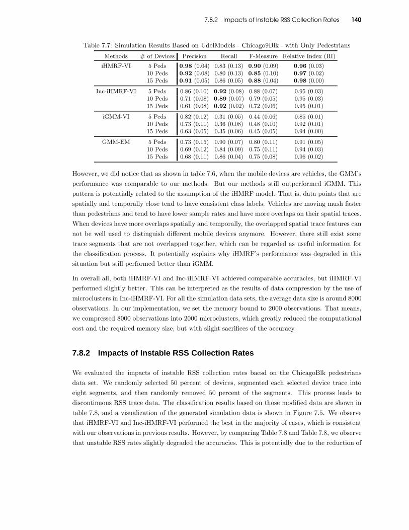
7.8.2 Impacts of Instable RSS Collection Rates 140
Table 7.7: Simulation Results Based on UdelModels - Chicago9Blk - with Only Pedestrians
Methods # of Devices Precision Recall F-Measure Relative Index (RI)
iHMRF-VI 5 Peds 0.98 (0.04) 0.83 (0.13) 0.90 (0.09) 0.96 (0.03)10 Peds 0.92 (0.08) 0.80 (0.13) 0.85 (0.10) 0.97 (0.02)15 Peds 0.91 (0.05) 0.86 (0.05) 0.88 (0.04) 0.98 (0.00)
Inc-iHMRF-VI 5 Peds 0.86 (0.10) 0.92 (0.08) 0.88 (0.07) 0.95 (0.03)10 Peds 0.71 (0.08) 0.89 (0.07) 0.79 (0.05) 0.95 (0.03)15 Peds 0.61 (0.08) 0.92 (0.02) 0.72 (0.06) 0.95 (0.01)
iGMM-VI 5 Peds 0.82 (0.12) 0.31 (0.05) 0.44 (0.06) 0.85 (0.01)10 Peds 0.73 (0.11) 0.36 (0.08) 0.48 (0.10) 0.92 (0.01)15 Peds 0.63 (0.05) 0.35 (0.06) 0.45 (0.05) 0.94 (0.00)
GMM-EM 5 Peds 0.73 (0.15) 0.90 (0.07) 0.80 (0.11) 0.91 (0.05)10 Peds 0.69 (0.12) 0.84 (0.09) 0.75 (0.11) 0.94 (0.03)15 Peds 0.68 (0.11) 0.86 (0.04) 0.75 (0.08) 0.96 (0.02)
However, we did notice that as shown in table 7.6, when the mobile devices are vehicles, the GMM’s
performance was comparable to our methods. But our methods still outperformed iGMM. This
pattern is potentially related to the assumption of the iHMRF model. That is, data points that are
spatially and temporally close tend to have consistent class labels. Vehicles are moving mush faster
than pedestrians and tend to have lower sample rates and have more overlaps on their spatial traces.
When devices have more overlaps spatially and temporally, the overlapped spatial trace features can
not be well used to distinguish different mobile devices anymore. However, there still exist some
trace segments that are not overlapped together, which can be regarded as useful information for
the classification process. It potentially explains why iHMRF’s performance was degraded in this
situation but still performed better than iGMM.
In overall all, both iHMRF-VI and Inc-iHMRF-VI achieved comparable accuracies, but iHMRF-VI
performed slightly better. This can be interpreted as the results of data compression by the use of
microclusters in Inc-iHMRF-VI. For all the simulation data sets, the average data size is around 8000
observations. In our implementation, we set the memory bound to 2000 observations. That means,
we compressed 8000 observations into 2000 microclusters, which greatly reduced the computational
cost and the required memory size, but with slight sacrifices of the accuracy.
7.8.2 Impacts of Instable RSS Collection Rates
We evaluated the impacts of instable RSS collection rates baesd on the ChicagoBlk pedestrians
data set. We randomly selected 50 percent of devices, segmented each selected device trace into
eight segments, and then randomly removed 50 percent of the segments. This process leads to
discontinuous RSS trace data. The classification results based on those modified data are shown in
table 7.8, and a visualization of the generated simulation data is shown in Figure 7.5. We observe
that iHMRF-VI and Inc-iHMRF-VI performed the best in the majority of cases, which is consistent
with our observations in previous results. However, by comparing Table 7.8 and Table 7.8, we observe
that unstable RSS rates slightly degraded the accuracies. This is potentially due to the reduction of

7.8.3 Impacts of Transmission Power Changes 141
Table 7.8: Unstable RSS Rates (UdelModels - Chicago9Blk - with Only Pedestrians)
Methods # of Devices Precision Recall F-Measure Relative Index (RI)
iHMRF-VI 5 Peds 0.91 (0.11) 0.77 (0.08) 0.83 (0.05) 0.93 (0.02)10 Peds 0.96 (0.05) 0.82 (0.11) 0.88 (0.08) 0.98 (0.02)15 Peds 0.84 (0.10) 0.83 (0.07) 0.83 (0.07) 0.98 (0.01)
Inc-iHMRF-VI 5 Peds 0.91 (0.17) 0.88 (0.15) 0.89 (0.15) 0.97 (0.04)10 Peds 0.77 (0.13) 0.86 (0.09) 0.81 (0.11) 0.95 (0.03)15 Peds 0.62 (0.10) 0.92 (0.02) 0.73 (0.07) 0.95 (0.02)
iGMM-VI 5 Peds 0.82 (0.13) 0.32 (0.07) 0.46 (0.09) 0.83 (0.02)10 Peds 0.71 (0.10) 0.31 (0.05) 0.43 (0.07) 0.91 (0.01)15 Peds 0.62 (0.09) 0.33 (0.06) 0.43 (0.06) 0.94 (0.01)
GMM-EM 5 Peds 0.75 (0.16) 0.90 (0.06) 0.81 (0.10) 0.90 (0.06)10 Peds 0.67 (0.08) 0.81 (0.07) 0.73 (0.04) 0.93 (0.02)15 Peds 0.71 (0.04) 0.82 (0.06) 0.76 (0.03) 0.96 (0.00)
samples size, since we have removed 50 percent of observations from 50 percent randomly selected
devices. However, as long as each segment is still composed of spatial and temporally adjacent data
points, the iHMRF model can be applied to capture the corresponding autocorrelations.
7.8.3 Impacts of Transmission Power Changes
Table 7.9: Change of Transmission Power (UdelModels - Chicago9Blk - with Only Pedestrians)
Methods # of Devices Precision Recall F-Measure Relative Index (RI)
iHMRF-VI 5 Peds 0.98 (0.02) 0.70 (0.07) 0.82 (0.06) 0.94 (0.02)10 Peds 0.95 (0.06) 0.77 (0.06) 0.85 (0.06) 0.97 (0.01)15 Peds 0.93 (0.04) 0.79 (0.05) 0.85 (0.02) 0.98 (0.00)
Inc-iHMRF-VI 5 Peds 0.76 (0.14) 0.98 (0.03) 0.85 (0.09) 0.93 (0.04)10 Peds 0.74 (0.12) 0.88 (0.08) 0.80 (0.09) 0.96 (0.02)15 Peds 0.58 (0.08) 0.86 (0.69) 0.69 (0.06) 0.95 (0.01)
iGMM-VI 5 Peds 0.83 (0.13) 0.31 (0.05) 0.45 (0.06) 0.85 (0.02)10 Peds 0.72 (0.11) 0.35 (0.07) 0.47 (0.09) 0.92 (0.01)15 Peds 0.65 (0.07) 0.35 (0.04) 0.45 (0.05) 0.94 (0.01)
GMM-EM 5 Peds 0.74 (0.11) 0.89 (0.04) 0.81 (0.07) 0.91 (0.04)10 Peds 0.63 (0.13) 0.83 (0.08) 0.71 (0.11) 0.93 (0.03)15 Peds 0.69 (0.04) 0.85 (0.04) 0.76 (0.02) 0.96 (0.00)
7.8.4 Comparisons on Precision, Recall, and F-Measure
Studies have been shown that attackers may hide their actual locations by periodically changing
the transmission powers of their mobile devices [258]. To simulate this behavior, we used the
ChicagoBlk pedestrians data set. Fifty percent of devices were selected, the trace of each selected
device was segmented into 8 same length pieces, and fifty percent of these pieces were shifted to
random directions with random spatial distances. The corresponding classification results are shown

7.8.5 Comparison on Time Costs 142
in Table 7.9. We observe that the changes of transmission power did not have significant impacts on
the accuracies. One potential interpretation is that the changes of transmission power will increase
the spatial entropy and hence make the devices’ corresponding traces more separated from other
traces. This will reduce the potential overlaps between device traces, and could even help improve
the accuracies of iHMRF-VI and Inc-iHMRF-VI.
7.8.5 Comparison on Time Costs
We evaluated the time costs of the four algorithms on three data sets, including ”1 Building 10
Floors” (7224 observations), ”Chicago9B1k with 10 Pedestrians and 10 Cars” (4525 observations),
and ”Chicago9B1k with 10 Pedestrians” (6000 observations). We set bucket size to 2000. That
means, the data will be processed bucket by bucket, 2000 observations each time. The results
are summarized in Figure 7.6. The X axis refers to the titles of the three data sets and the Y
axis refers to running duration (seconds). We can observe that our proposed incremental inference
algorithm Inc-iHMRF-VI is much more efficient than the offline inference algorithm iHMRF-VI. Our
algorithm Inc-iHMRF-VI is even faster than iGMM. This indicates an significant improvement on
the computational efficiency. The savings on time cost by Inc-iHMRF-VI will become greater when
the data size increases. Note that, GMM has the lowest time cost. However, since GMM does not
need to automatically estimate the number of clusters. Its time complexity should be much smaller
than iGMM and iHMRF.
1 Building 10 Floors Chicago9B1k−Peds−Cars Chicago9B1k−Peds0
20
40
60
80
100
120
140
160
iHMRF−VIiGMMGMMInc−iHMRF−VI
Figure 7.6: Comparison on Time Costs (Seconds)
7.8.6 A Case Study on Detecting Masquerade Attacks
This section presents a case study on masquerade attacks detection, which is one of the most dan-
gerous attack types. A masquerade attack refers to the attacking behavior where an attacker im-
personates an authorized user of a system by using a faked identity (e.g., MAC address) in order to

7.9 Conclusion 143
gain access to unauthorized personal resources. In order to simulate this attack behavior, we used
the ChicagoBlk pedestrians data set and the 1-Building-10-Floors data set, and randomly selected
k clusters and set their cluster identities into an identical cluster identity. By using fingerprinting
techniques, this type of attackers can be identified if we discover that multiple clusters share the
same identity information. Here k refers to the number of masquerade devices. We considered differ-
ent settings of k, from 3 to 6, and evaluated the related detection rates based on different detection
methods. The results are summarized in Table 7.8.6. The results indicate that our framework (by
either iHMRF-VI or Inc-iHMRF-VI) achieved the highest detection rate in most cases. The GMM
method performed slightly than Inc-iHMRF-VI and iHMRF-VI. However, here we used the true
number of clusters as the initial setting for the GMM method. In real applications, where the actual
number is unknown, the GMM method will perform much worse.
Peds Cars Att. iHMRF Inc-iHMRF iGMM GMM# # # -VI -VI
10 10 3 0.98 0.81 0.46 0.7610 10 4 0.97 0.84 0.55 0.8110 10 5 0.97 0.87 0.62 0.8410 10 6 0.97 0.88 0.67 0.8615 15 3 0.97 0.86 0.62 0.8515 15 4 0.97 0.85 0.62 0.8515 15 5 0.97 0.86 0.64 0.8615 15 6 0.97 0.87 0.66 0.87
Table 7.10: Detection Rates for MasqueradeAttacks Based on UdelModels - Chicago9B1k -
Pedestrains
Peds Cars Att. iHMRF Inc-iHMRF iGMM GMM# # # -VI -VI
10 0 3 0.71 0.86 0.44 0.7610 0 4 0.85 0.89 0.72 0.9410 0 5 0.89 0.91 0.73 0.8810 0 6 0.93 0.98 0.87 0.9515 0 3 0.80 0.60 0.36 0.6815 0 4 0.85 0.86 0.56 0.8715 0 5 0.88 0.86 0.65 0.8815 0 6 0.95 0.91 0.78 0.93
Table 7.11: Detection Rates for MasqueradeAttacks on UdelModels - Chicago9B1k - 1 Building
10 Floors
7.9 Conclusion
Device fingerprinting is a fundamental problem for wireless network security. Passive fingerprinting
techniques are effective since they are designed based on device-dependent features (e.g., RSS, AOD,
and TOA) that attackers can not manipulate. However, existing solutions can only support either
time-dependent or time-independent features, but no methods can handle both. This paper presents
the first unified fingerprinting approach based on infinite hidden Markov random field (iHMRF). It
is able to model both time-independent and time-dependent features concurrently and is able to
automatically detect the number of devices. We present a novel incremental classification algorithm
that is suitable for a streaming environment with limited memory and computational resources. Ex-
tensive numerical analysis further validated the effectiveness and efficiency of our proposed approach.
For our future work, we are planning to evaluate the performance of our proposed approach in real
life devices. We will also extend our approach to handle other related wireless security problems,
such as the identification of primary and secondary users to prevent dynamic spectrum access and
malicious behavior attacks in cognitive radio networks.

7.9 Conclusion 144
Figure 7.7: Visualization for the UdelModels Data with 1 Building 10 Floors

7.9 Conclusion 145
Figure 7.8: Visualization for the UdelModels - Chicago9B1k Data with Pedestrians and Cars

7.9 Conclusion 146
Figure 7.9: Visualization for the UdelModels - Chicago9B1k Data with Only Cars

Chapter 8 147
Chapter 8
Achievements andFuture Work
8.1 Achievements
In this thesis, I presented a number of efficient algorithms for mining large spatio-temporal data for a
variety of application domains, such as medical imaging, urban traffic prediction, weather forecasting,
and social networks. First, we proposed a generalized local statistical model for spatial outlier
detection, which is more accurate and computationally efficient than existing methods (Chapter
3). Second, we developed a reduced space dimension reduction model combined with an artificial
Student-t based random buffering process for detecting outliers in non-numerical data (Chapter 4).
Third, we presented a robust spatio-temporal random effects model and designed efficient algorithms
that can do robust spatio-temporal prediction in near-linear time (Chapter 5). Third, we developed
a generic hidden Markov model based approach to inferring hidden human activities that associate
with residential energy consumption data collected from smart meters (Chapter 6). Finally, we
presented a novel application of infinite Markov random field to the passive device fingerprinting
problem in the wireless security field and developed a new online learning algorithm for the streaming
environment in wireless networks (Chapter 7).
Spatial Outlier Detection (Chapter 3 and Chapter 4)
Spatial novelty patterns, or spatial outliers, are those observations whose characteristics are markedly
different from their spatial neighbors. There are two major branches of spatial outlier detection
(SOD) methodologies, including the global Kriging based and the local Laplacian smoothing based.
The former approach was designed based on robust statistics and the popular Kriging framework.
This approach is very effective, but has a low efficiency with a time complexity O(N4), where N is the
data cardinality. The latter approach applied Laplacian smoothing to eliminate spatial dependencies
between observations, and then converted the SOD problem into a general outlier detection problem.

8.1 Achievements 148
This approach has the time complexity of O(N2), but it implicitly assumes that the observations
modified by Laplacian smoothing are identically and independently distributed (i.i.d) and follow a
Gaussian distribution. In addition, these approaches were designed for numerical attributes, and
the large scale SOD problems for other data types, such as count, binary, and categorial attributes,
have not been well explored. We considered two open problems as follows:
1. Will the Laplacian smoothing process generate i.i.d. Gaussian observations?
2. How can numerical SOD methods be generalized to non-numerical data types, such as count,
binary, and categorial data?
To address the first problem, we theoretically and empirically validated the effectiveness of Laplacian
smoothing for the elimination of spatial autocorrelations, based on popular autocorrelation settings
(e.g., gaussian and exponential kernels). This work provides fundamental support for the family of
local based methods. However, we also discovered a side effect of Laplacian smoothing in that this
process generates an extra spatial autocorrelation variation to the data due to the convolution effects
between measurement errors. To capture this extra variability, we proposed a Generalized Local
Statistical (GLS) framework, and designed two improved forward and backward SOD methods [308],
which outperformed existing SOD methods in a number of simulation and real data sets.
We addressed the second problem by using generalized spatial linear models, which map observations
of different data types to latent numerical variables via a link function. Existing SOD techniques can
then be applied to latent numerical variables. In our optimized design, we first applied a Bayesian
generalized spatial linear model to capture spatial correlations for different data types, such as count,
binary, ordinal, and nominal. We then integrated an additional “error buffer” component based on
Student-t distribution to capture large variations caused by outliers. After that, we considered a
latent reduced-rank spatial Kriging model and designed an approximate inference algorithm that
has a linear time complexity. We have also proposed solutions to spatial categorical SOD [303],
multivariate SOD [314,300], local spatial outlier cluster detection [307], spatial anomaly trajectory
detection in a transportation network [310], and an entropy based method for assessing the number
of spatial outliers [312].
Robust Prediction for Large Spatio-Temporal Data (Chapter 5)
The spatio-temporal datasets being collected nowadays are usually in Gigabyte or even Terabyte
scale. In existing related work, only a limited number of methods have the ability to conduct efficient
spatio-temporal prediction in linear time, but these methods are still limited to Gaussian data. It
is challenging to deal with massive spatiotemporal datasets that are noisy and non-Gaussian. One
effective direction to address this challenge is the generalization of existing methods to make them
more robust when a small portion of data objects deviate from the distribution assumption. We
consider two open problems as follows
1. Is it possible to conduct robust offline spatio-temporal prediction in near linear time?

8.1 Achievements 149
2. Is it possible to conduct robust online spatio-temporal prediction in near linear time?
We proposed a robust version of the Spatio-Temporal Random Effects (STRE) model, namely the
Robust STRE (R-STRE) model. The regular STRE model is a recently proposed statistical model
for large spatio-temporal data that has a linear order time complexity. However, the STRE model
has been shown sensitive to outliers or anomaly observations. Our R-STRE model is more resilient
to outliers or other small departures from model assumptions. Specifically, the R-STRE model
assumes that the measurement error follows a heavy-tailed distribution, such as Huber and Laplace
distributions, instead of a traditional Gaussian distribution. This extension leads to non-analytical
solutions to inferences, such as smoothing, filtering, and forecasting. We proposed near-linear-time
primal-dual interior point algorithms to calculate the Maximum-A-Posterior (MAP) estimates and
applied Laplace approximations to calculate the uncertainty estimates (variance-covariance matrix)
for robust inferences. The theoretical properties of the proposed R-STRE model and its connection
with the regular STRE model were also explored. We also developed a related robust prediction
framework for large spatial data using integrated Gaussian and Laplace approximation techniques
[318].
The preceding approach only provides a solution to the spatio-temporal smoothing problem, which
aims to predict missing vlaues in historical data. It can not be directly applied to conduct efficient
online filtering and forecasting. In order to address this problem, we proposed an alternative ap-
proach [317] using backward and forward message passing to support incremental inference. This
approach can be efficiently implemented using a state-of-the-art approximate inference technique,
named expectation propagation, combined with a Student-t distribution to model the measurement
error. One of the main challenges using approximate inference is to address the high dimension-
ality challenge, that is, the posterior distribution of a large number of latent variables needs to
be approximated. We proposed a novel approximate inference approach, which approximates the
model into the form (we called approximate R-STRE model) that separates the high dimensional
latent variables into groups, and then estimates the posterior distributions of different groups of
variables separately in the framework of Expectation Propagation. We presented theoretical evalu-
ations to show that our solution based on the approximate R-STRE model becomes equivalent to
the traditional R-STRE model when the degree of freedom of the Student-t distribution is set to
infinite.
Energy Disaggregation (Activity Analysis) using Smart Meter Data (Chapter 6)
Sustainability and design of sustainable technologies have become urgent and important priority for
cities given the unprecedented level of resource demand - water, energy, transit, healthcare, public
safety - to every imaginable service that makes a city attractive and desirable. With the widespread
deployment of smart grid and smarter cities, smart meters have been installed in households and
industry buildings to measure the aggregated resource consumptions (e.g., power, water, and gas).
Energy disaggregation aims to disaggregate smarter meter data into the energy consumptions of
individual appliances, such as washer, refrigerator, laptop, and lighting. Studies have shown that
providing users appliance-level energy information can cause users to save significant amount of

8.1 Achievements 150
energy. Smart meter data usually has a low sampling frequency (e.g., one reading per 15 minutes
or 1 hour). This special feature makes most existing disaggregation techniques inappropriate, such
as Independent Component Analysis (ICA) used in audio source separation. Energy disaggregation
based on low frequency data is an emerging field that starts from early 2010. As one of the pioneers,
we collaborate with a group at IBM Research and work on three open problems as follows:
1. Is it possible to disaggregate lower frequency water smart meter data?
2. Is it possible to disaggregate lower frequency power smart meter data?
To address the first problem, we proposed a general statistical framework that disaggregates water
consumptions on coarse granular smart meter readings by modeling fixture characteristics, household
behavior, and activity correlations [304]. This framework is composed of six components, including
event extraction, model selection and training, parallel activity detection, parallel size estimation,
hidden activity identification, and consumption decomposition. We showed that if the event extrac-
tion is accurate, and the stochastic model is accurately selected and trained, our framework will lead
to a maximum-a-posterior solution for the disaggregation. Also, each component can be customized
for different application scenarios, which makes the framework very flexible and applicable. This
framework has been used in the first smarter city project of the united states, deployed by IBM to
the city of Dubuque in 2011. By a recent study conducted based a controlled group of 152 houeholds
and a noncontrolled group of 151 households for 9 weeks, the smarter city project achieved water
savings of 89,090 gallons (6.6%) for 9 weeks and 151 households.
To address the second problem (power energy disaggregation), we explored an alternative strategy
based on an energy disaggregation approach via discriminative sparse coding (DDSC) [306]. DDSC
aims to learn a unique disaggregation model for all households. We observed that this strategy is in-
appropriate, because different households may have different appliances and power usage habits. We
first reformulated DDSC as a generative statistical model, and then proposed a improved Bayesian
version of DDSC [319], in which we integrated household dependent information into the disaggrega-
tion framework, such as appliance information and power usage behaviors. Based on the improved
model, we proposed an efficient disaggregation algorithm by using variational inference techniques.
Wireless Device Fingerprinting (Chapter 7)
Wireless device fingerprinting is a fundamental problem for wireless security. Existing solutions have
been focused on either spatio-temporal independent features (e.g., phase shift difference, frequency
difference) or spatio-temporal dependent features (e.g., radio signal strength (RSS), time difference
of arrival (TDOA)). However, no works have been done to consider all useful features concurrently.
We presented a unified framework for the fingerprinting problem based on infinite hidden Markov
random field. Our framework is able to model both spatio-temporal independent and spatio-temporal
dependent features and is able to automatically detect the number of devices. We proposed the first
incremental classification algorithm for the iHMRF model that is suitable for the wireless streaming
environment that has limited memory and computational resources.

8.2 Future Work 151
8.2 Future Work
This section discusses important directions of the following topics for future work, including spatial
and spatio-temporal outlier detection, spatio-temporal anomalous cluster detection, energy disag-
gregation, and wireless device fingerprinting.
8.2.1 Spatial and Spatio-Temporal Outlier Detection
We have presented two generic solutions to the problems of numerical and non-numerical spatial
outlier detection. However, there are still a limited number of methods that can effectively and effi-
ciently detect outliers from large scale multivariate mixed type spatial datasets and spatio-temporal
datasets. For multivariate mixed type spatial datasets, there are three main challenges: 1) How to
model spatial correlations between mixed type attributes; 2) How to model large variations caused
by outliers; 3) How to detect outliers in a near linear time cost?
To address the first challenge, the mixed-type attributes can be mapped to latent numerical random
variables that are multivariate Gaussian in nature. Each attribute is mapped to a corresponding
latent numerical variable via a specific link function, such as a logit function for binary attributes,
and a log function for count attributes. Using link functions to model attributes of different types
is one of the most popular strategies for modeling non-numerical data. Based on this strategy, the
dependency between mixed type attributes is modeled by dependencies between their latent numer-
ical random variables using a variance-covariance matrix. To address the second challenge we may
employ a similar idea used in our approach for non-numerical outlier detection. An additional error
buffer component based on heavy tailed distributions, such as Student-t and Laplace distributions,
can be incorporated to capture large variations caused by anomalies. For the third challenge, we
can apply fixed rank or knot based dimension reduction techniques. Because the inference of the
resulting model is analytically intractable, approximate inference techniques need to be used, such
as interior point methods, Gaussian approximation, Laplace approximation, variational inference,
and expectation propagation.
For the problem of spatio-temporal outlier detection, one important subproblem is the detection of
non-numerical univariate outliers. There are two spatio-temporal models that can be used, including
the spatio-temporal random effects model (STRE) model and the spatio-temporal Kriging (STK)
model. In our work, we have demonstrated the effectiveness and efficiency of the detection methods
designed based on heavy tailed distributions. Here, we can consider a similar framework and add an
additional random variables that follow a heavy tailed distribution to absorb large variations caused
by outliers. One additional challenge is to consider both spatial and temporal correlations, which
make the design of efficient approximate inference algorithms more difficult. Another important
problem is the detection of multivariate mixed type outliers. We can use a similar strategy discussed
above for multivariate spatio-temporal data. Lastly, currently all the proposed algorithms are focused
on the detection of two-sided outliers. However, one-sided outliers are also very important. We are
planning to further extend our proposed algorithms such that one-sided outliers can also be identified.

8.2.2 Spatio-Temporal Anomalous Cluster Detection 152
8.2.2 Spatio-Temporal Anomalous Cluster Detection
Anomalous spatial cluster detection is different from general spatial outlier detection. The latter
focuses on the detection of isolated outliers, but the former focuses on the detection of a group
of outliers that are spatial neighbors to each other. The additional constraint of spatial affinity
between outliers makes spatial cluster detection more challenging. In previous years, a number of
works have been done for the detection of spatial clusters. One of the major approaches is the
so-called spatial scan statistics. This approach is very effective, but the computational cost is very
high and it is unable to detect irregularly shaped spatial clusters. To address these two challenges,
Neill et.al. [77–82] proposed fast subset scan and Bayesian scan statistics approaches.
Based on our previous work, there are several directions that can be explored to further improve the
performance of existing methods. First, the family of scan statistics based approaches assumes that
the trend of the data has been eliminated in advance. However, this may not be practical in a dy-
namic environment, in which the trend model needs to fitted concurrently with the process of spatial
cluster detection. In this situation, the scan statistics based approaches may be in inappropriate.
This challenge can be potentially addressed by using our proposed models based on heavy tailed
distributions. In our previous approaches, we assume that the error-buffer random variables that
follow a heavy tailed distribution are i.i.d. In order to identify the group of outliers that are spatial
neighbors to each other, we can further add an additional latent layer to these error-buffer random
variables, that forms a latent Markov random field, which uses the so-called Markov Property to
have consistent labels (normal or outlier) for neighbor observations.
The second direction is to consider the detection of anomalous clusters in heterogenous data. For
example, in order to detect social unrest events from social media, which includes spatial attributes,
temporal attributes, and many other types of attributes, it is necessary to extend traditional spatial
clustering techniques to support spatial, temporal, textual, and graph data attributes together.
Two potential strategies may be explored to address this challenge. The first strategy is to integrate
topic model and spatio-temporal random effects (or Kriging) model into an unified framework,
which makes is possible to model both spatio-temporal and textual data. The second strategy is
to integrate sliding window based techniques and scan statistics together. For each sliding window,
the potential spatial clusters and graph clusters are identified. Then for adjacent sliding windows,
the clusters that share the same locations, or textual content, or graph nodes are connected, and
then we are able to monitor the evolution patterns of clusters, and detect or even forecast significant
spatio-temporal clusters.
8.2.3 Energy Disaggregation
Energy disaggregation based on smarter meter data is a relatively new research topic that began
in last five years. Smart meter data usually has a low sampling frequency (e.g., one reading per 15
minutes or 1 hour). This special feature makes most traditional time series disaggregation techniques
inappropriate, such as the Independent Component Analysis (ICA) technique used in audio source

8.2.4 Wireless Device Fingerprinting 153
separation. In our previous work, we have presented an effective approach to the disaggregation of
water data based on HMM. For our future work, we are interested to explore two directions.
First, there are usually multiple types of energy consumption data that need to be disaggregated,
such as water, gas, and power, and these different types of data may have significant correlations
to each other. For example, a shower activity may concurrently consume both water and gas (or
power) resources, and a washer or diswasher usage may concurrently consume both water and
power resources. To address this challenge, we can extend the traditional factorial hidden Markov
model (FHMM) and consider an improved model, namely Parallel Factorial Hidden Markov Model
(P-FHMM). P-FHMM models each type of energy data via an individual FHMM model. The
multiple FHMM models are coupled together by considering dependencies between appliances of
different energy types. For example, washer-dryer will concurrently consumer power, water, and
gas; dishwaser will consume both power and water; and shower and toliet uses are closely correlated
with restroom lightening. In order to consider household dependent features, a Bayesian version of
the P-FHMM model (BP-FHMM) can be designed, in which users will be able to add household
dependent features (e.g., appliances profiles and energy usage habits) as priors of the state transition
and emission distribution parameters. Structured variational inference algorithms can be applied to
do multi-energy disaggregation based on P-FHMM and BP-FHMM models.
Second, in order to learn a FHMM model, it is required to collect a training set in advance for each
household that has the disaggregated consumption data of individual appliances, because different
households may have different appliances and consumption behaviors. However, this may be imprac-
tical since the collection of energy consumption data is not only label-extensive but also may cause
a lot of concerns on human privacy leaks. Therefore, it is important to developed a semi-supervised
model that can be trained based on the data collected from a limited number of households, and can
be directly applied the other households as well. Specifically, the goal is to learn a model based on
a small set of labeled data but a huge set of unlabeled data. An alternative approach is to consider
active learning techniques. Specifically, we first learn a model based on a small set of training data.
Then we apply the trained model to identify a small set of new streamed data to ask users to provide
labels, such that the model can be adapted to the change of appliances or users’ energy consumption
behaviors. Lastly, the proposed algorithms are mostly focused the temporal dimension. However,
smarter meter data also has the important spatial dimension. We are interested to study the energy
disaggregation problem based in both spatial and temporal dimensions.
8.2.4 Wireless Device Fingerprinting
As discussed in Chapter 7, we proposed an infinite hidden Markov random field model (iFHMM)
to capture correlations between both time-independent and time-dependent features. The iFHMM
model helps make spatial and temporal neighbors with a consistent cluster (device) label, but it
does not have the ability to differentiate the objects that are spatially far away, but temporally
close, using different cluster labels. For the problem of device fingerprinting, if two objects are in
this situation, they tend to origin from two different devices, because a device can not occur in

8.3 Published Papers 154
two different places at the same time. In order to address this challenge, the FHMM model can be
extended to consider the preceding additional constraint. In addition, the iFHMM model is unable to
explicitly model the dynamic pattern (e,g., spatial trajectory of RSS features), since it only has the
spatial infinity constraint. An alternative approach is to consider Spatial Temporal Kalman Filtering
(STKF) model, which has been widely used for predicting spatial trajectories. Another interesting
research problem is to apply the iFHMM or STKF model and hypothesis testing based techniques
to detect if a device changes locations within a specified time interval, for example, moving from
inside building to outside building.
8.3 Published Papers
1. Feng Chen, Jing Dai, Bingsheng Wang, Sambit Sahu, Milind Naphade, Chang-Tien Lu,“Activity
Analysis Based on Low Sample Rate Smart Meters,” Proceedings of the 17th ACM SIGKDD
International Conference on Knowledge Discovery and Data Mining (ACM-KDD), pages
240-248, 2011 (Acceptance rate: 17.5%)
2. Feng Chen, Chang-Tien Lu, Arnold P. Boedihardjo,“GLS-SOD: A Generalized Local Statis-
tical Approach for Spatial Outlier Detection,” Proceedings of the 16th ACM SIGKDD Interna-
tional Conference on Knowledge Discovery and Data Mining (ACM-KDD), pages 1069-1078,
2010 (Acceptance rate: 13%)
3. Feng Chen, Chang-Tien Lu, Arnold P. Boedihardjo,“On Locally Linear Classification by Pair-
wise Coupling,” Proceedings of the IEEE International Conference on Data Mining (IEEE
ICDM), pages 749-754, 2008 (Acceptance rate: 19%)
4. Feng Chen and Chang-Tien Lu, ”Nearest Neighbor Query,” Encyclopedia of Geographical
Information Science (1st Edition),
5. Feng Chen, Jaime Arredondo, Rupinder Paul Khandpur, Chang-Tien Lu, David Mares,
Dipak Gupta, and Naren Ramakrishnan,” Spatial Surrogates to Forecast Social Mobilization
and Civil Unrests,” Position Paper in CCC Workshop on “From GPS and Virtual Globes to
Spatial Computing-2012,” Washington, D.C., Sep 2012
6. Yang Chen, Feng Chen, Jing Dai, T. Charles Clancy, ”Student-t Based Robust Spatio-
Temporal Prediction,” the IEEE International Conference on Data Mining (IEEE ICDM),
2012 (Full paper, Acceptance rate 10.7%)
7. Xutong Liu, Feng Chen, Chang-Tien Lu, ”Robust Inference and Outlier Detrection for Large
Spatial Data Sets,” the IEEE International Conference on Data Mining (IEEE ICDM), 2012
(Full paper, Acceptance rate 10.7%)
8. Bingsheng Wang, Feng Chen, Haili Dong, Arnold Boedihardjo, and Chang-Tien Lu, ”Low-
Sample-Rate Water Consumption Disaggregation via Sparse Coding with Extended Discrimi-

8.3 Published Papers 155
native Dictionary,” the IEEE International Conference on Data Mining (IEEE ICDM), 2012
(Short paper, Acceptance rate 20%)
9. Jing Dai, Feng Chen, Sambit Sahu, Milind Naphade,“Regional Behavior Change Detection
via Local Spatial Scan,” Proceedings of the 18th ACM SIGSPATIAL International Conference
on Advances in Geographic Information Systems (ACM SIGSPATIAL GIS), 2010
10. Xutong Liu, Chang-Tien Lu, Feng Chen,“Spatial Outlier Detection: Random Walk Based
Approaches,” Proceedings of the 18th ACM SIGSPATIAL International Conference on Ad-
vances in Geographic Information Systems (ACM SIGSPATIAL GIS), 2010 (Acceptance
rate: 21%)
11. Xutong Liu, Chang-Tien Lu, Feng Chen,“Spatial Categorical Outlier Detection: Pair Corre-
lation Function Based Approach,” Proceedings of the 19th ACM SIGSPATIAL International
Conference on Advances in Geographic Information Systems (ACM SIGSPATIAL GIS),
to appear 2012
12. Qiben Yan, Ming Li, Feng Chen, Tingting Jiang, Wenjing Lou, Chang-Tien Lu, ”Optimal
Network Traffic Surveillance in Cognitive Radio Networks,” The 32nd IEEE International
Conference on Computer Communications (IEEE INFOCOM), 2013 (Acceptance rate 17%)
13. Arnold P. Boedihardjo, Chang-Tien Lu, Feng Chen,“A Framework for Estimating Complex
Probability Density Structures in Data Streams,” Proceedings of the ACM 17th Conference on
Information and Knowledge Management (ACM CIKM), pages 619-628, 2008 (Acceptance
rate: 17%)
14. Chang-Tien Lu, Arnold P. Boedihardjo, David Dai, Feng Chen,“HOMES: Highway Opera-
tions and Monitoring and Evaluation System,” ACM 16th International Conference on Ad-
vances in Geographic Information Systems (ACM SIGSPATIAL GIS), Poster Paper, pages
529-530, 2008
15. Dechang Chen, Chang-Tien Lu, Yufeng Kou, Feng Chen,“On Detecting Spatial Outliers,”
Journal of Geoimformatica, vol. 12, pages 455-475, 2008
16. Qifeng Lu, Feng Chen, Kathleen Hancock,“On Path Anomaly Detection in a Large Trans-
portation Network,” Journal of Computers, Environment and Urban Systems, vol. 33, pages
448-462, 2009
17. Yao-Jan Wu, Feng Chen, Chang-Tien Lu, Brian Smith, Yang Chen,“Traffic Flow Prediction
for Urban Network using Spatial Temporal Random Effects Model,” the 91st Annual Meeting
of the Transportation Research Board (TRB), to appear 2012
18. Jing Dai, Ming Li, Sambit Sahu, Milind Naphade, Feng Chen,“Multi-granular Demand Fore-
casting in Smarter Water,” Proceedings of the 13th International Conference on Ubiquitous
Computing (Ubicomp), Poster Paper, 2011

8.3 Published Papers 156
19. Xutong Liu, Chang-Tien Lu, and Feng Chen,“An Entropy-Based Method for Assessing the
Number of Spatial Outliers,” IEEE International Conference on Information Reuse and Inte-
gration (IRI), pages 244-249, 2008 Springer-Verlag, pages 776-781, 2008

Appendix A 157
Appendix A
Appendix
A.1 Estimated Bound
Theorem 3 presents an upper bound of the absolute correlation function |ρ(ω∗i , ω
∗j ;θθθ)|. The prop-
erties of this upper bound function are demonstrated in Figures [A.1-A.5], where we consider five
representative cases with c = 6, 11, 15, 2, 40, respectively. The X axis refers to the row difference
between sj and si: row(sj) − row(si). The Y axis refers to the column difference between sj and
si : col(sj) − col(si). The Z axis refers to the absolute correlation value. Each figure includes two
surfaces. The surface with colored (yellow to red) map refers to the surface calculated by the esti-
mated upper bound function. The surface in gray color scale refers to the surface calculated by the
true correlation function (see equation 3.17). These results demonstrate that the estimated upper
bound function is a tight upper bound of the true absolute correlation function |ρ(ω∗i , ω
∗j ;θθθ)|.
A.2 Definition of Matrices M and E
The matrices M and E are defined as follows:
M = CTC,E = CTa,
where a =[
−U− 1
21 H1η0,0, · · · ,0
]T
, η0 refers to the initial value and is predefined, and
C =
U− 1
21 0 · · · 0 0
−U− 1
22 H2 U
− 12
2 · · · 0 0...
......
...
0 0 · · · U− 1
2
T−1 0
0 0 · · · −U− 1
2
T HT U− 1
2
T
.

A.2 Definition of Matrices M and E 158
Figure A.1: The comparison between the true correlation |ρ(ω∗i , ω
∗j ;θθθ)| and the estimated bound
function. Here, K = 12, c = 6.
Figure A.2: The comparison between the true correlation |ρ(ω∗i , ω
∗j ;θθθ)| and the estimated bound
function. Here, K = 12,c = 11.

A.2 Definition of Matrices M and E 159
Figure A.3: The comparison between the true correlation |ρ(ω∗i , ω
∗j ;θθθ)| and the estimated bound
function. Here, K = 12,c = 15.
Figure A.4: The comparison between the true correlation |ρ(ω∗i , ω
∗j ;θθθ)| and the estimated bound
function. Here, K = 12,c = 20.

A.3 Proof of Theorem 2 160
Figure A.5: The comparison between the true correlation |ρ(ω∗i , ω
∗j ;θθθ)| and the estimated bound
function. Here, K = 12,c = 40.
It can be readily derived that
1
2
T∑
t=1
(ηt − Htηt−1)TU−1
t (ηt − Htηt−1)
=1
2(a + Cη)T (a + Cη) =
1
2ηT Mη + ETη +
1
2aT a.
A.3 Proof of Theorem 2
The dual function g(ω) is defined as
g(ω) = infη,ξ,r
L(η, ξ, r,ω) = infη,r,ξ
1Tϕ(r) +1
2ηT Mη + ETη +
1
2ξTΛξξ + ωT (r + OSη + Oξ − Z).
Fixing r and solving the system of liner questions
∇L(η, ξ, r,ω)
∇η= Mη + ST OTω + E = 0,
∇L(η, ξ, r,ω)
∇ξ= Λξξ + OTω = 0,
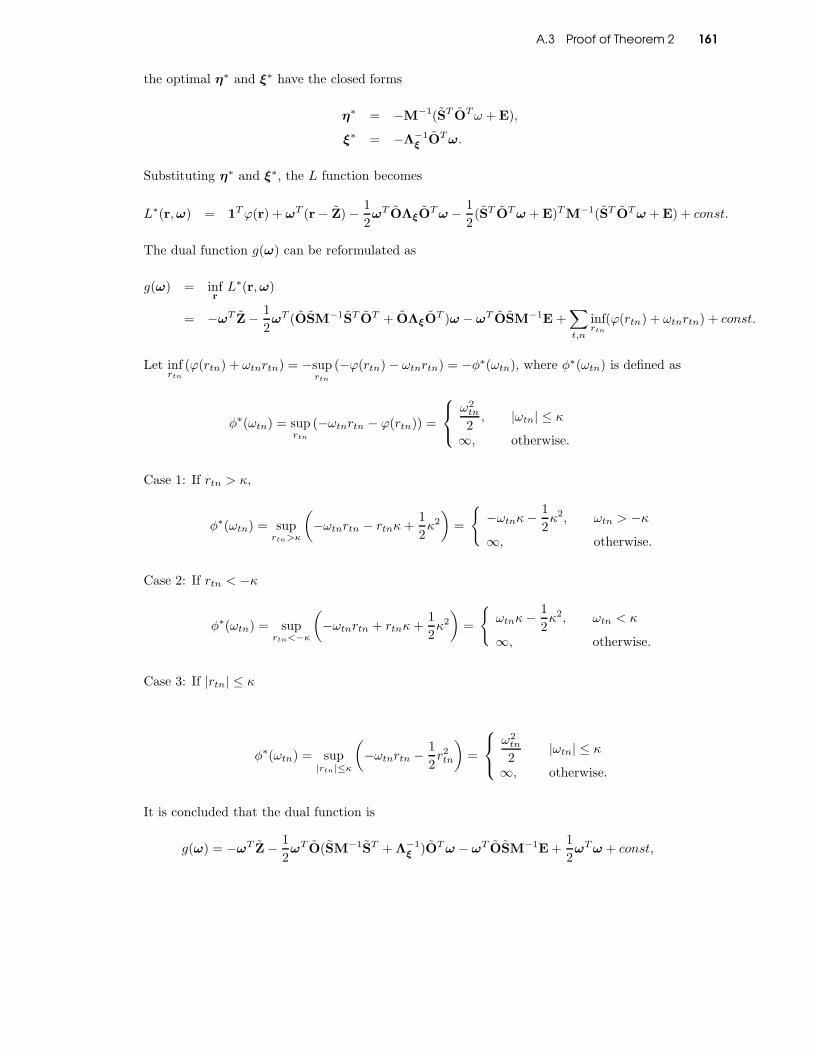
A.3 Proof of Theorem 2 161
the optimal η∗ and ξ∗ have the closed forms
η∗ = −M−1(ST OTω + E),
ξ∗ = −Λ−1ξ OTω.
Substituting η∗ and ξ∗, the L function becomes
L∗(r,ω) = 1Tϕ(r) + ωT (r − Z) −1
2ωT OΛξO
Tω −1
2(ST OTω + E)TM−1(ST OTω + E) + const.
The dual function g(ω) can be reformulated as
g(ω) = infrL∗(r,ω)
= −ωT Z −1
2ωT (OSM−1ST OT + OΛξO
T )ω − ωT OSM−1E +∑
t,n
infrtn
(ϕ(rtn) + ωtnrtn) + const.
Let infrtn
(ϕ(rtn) + ωtnrtn) = −suprtn
(−ϕ(rtn) − ωtnrtn) = −φ∗(ωtn), where φ∗(ωtn) is defined as
φ∗(ωtn) = suprtn
(−ωtnrtn − ϕ(rtn)) =
ω2tn
2, |ωtn| ≤ κ
∞, otherwise.
Case 1: If rtn > κ,
φ∗(ωtn) = suprtn>κ
(
−ωtnrtn − rtnκ+1
2κ2
)
=
−ωtnκ−1
2κ2, ωtn > −κ
∞, otherwise.
Case 2: If rtn < −κ
φ∗(ωtn) = suprtn<−κ
(
−ωtnrtn + rtnκ+1
2κ2
)
=
ωtnκ−1
2κ2, ωtn < κ
∞, otherwise.
Case 3: If |rtn| ≤ κ
φ∗(ωtn) = sup|rtn|≤κ
(
−ωtnrtn −1
2r2tn
)
=
ω2tn
2|ωtn| ≤ κ
∞, otherwise.
It is concluded that the dual function is
g(ω) = −ωT Z −1
2ωT O(SM−1ST + Λ−1
ξ )OTω − ωT OSM−1E +1
2ωTω + const,

A.4 Proof of Theorem 3 162
when |ω| ≤ κ1; and −∞, otherwise.
A.4 Proof of Theorem 3
The dual function g(ω) is defined as
g(ω) = infη,ξ,r
L(η, ξ, r,ω)
= infη,r,ξ
1T ‖r‖1 +1
2ηTMη + ETη +
1
2ξTΛξξ + ωT (r + OSη + Oξ − Z).
Fixing r, similar to the Huber distribution case, the optimal η∗ and ξ∗ have the closed forms
η∗ = −M−1(ST OTω + E),
ξ∗ = −Λ−1ξ OTω.
Substituting η∗ and ξ∗, the dual function can be reformulated as
g(ω) = −ωT Z−1
2ωT (OSM−1ST OT + OΛξO
T )ω − ωT OSM−1E + infr
(
‖r‖1 + ωT r)
+ const.
It can be readily proved that
infr
(
‖r‖1 + ωT r)
=
0, −1 ≤ ω ≤ 1
−∞, otherwise.
It is concluded that the dual function
g(ω) = −ωT Z −1
2ωT O(SM−1ST + Λ−1
ξ )OTω − ωT OSM−1E + const,
when 1 ≤ ω ≤ 1; g(ω) = −∞, otherwise.

A.5 Offline Inference Solution for iHMRF 163
A.5 Offline Inference Solution for iHMRF
The variational parameters are estimated as follows:
ζc,1 = 1 +
N∑
i=1
q(zi = c) (A.1)
ζc,2 =λ1
λ2
+
C∑
k=c+1
N∑
i=1
q(zi = k) (A.2)
λ1 = λ1 + C − 1 (A.3)
λ2 = λ2 −C−1∑
c=1
(ψ(ζc,2) − ψ(ζc,1 + ζc,2)) (A.4)
wc =N∑
i=1
q(zi = c) (A.5)
xc =
∑Ni=1 q(zi = c)xi
wc(A.6)
Ξ =
N∑
i=1
q(zi = c)(xi − xc)(xi − xc)T (A.7)
υc = υc + wc (A.8)
ηc = ηc + wc (A.9)
gc =υcgc + wcxc
υc(A.10)
Λc =υcwc
υc + wc(gc − xc)(gc − xc)
T + Λc
+Ξc (A.11)
q(xi = c) ∝ p(xi = c|(N)(xi); γ)πc(β)p(xi|Θc) (A.12)
πc(β) = exp
(
c−1∑
k=1
ψ(ζk,2) − ψ(ζk,1 + ζk,2)
)
× exp (ψ(ζc,1) − ψ(ζc,1 + ζc,2)) (A.13)
p(xi|Θc) = exp
−1
2log |
Λc
2| +
1
2
d∑
k=1
ψ(υc + 1 − k
2)
× exp
−1
2υc(xi − gc)
T Λ−1c (xi − gc)
× exp
−d
22π −
d
2ηc
(A.14)

BIBLIOGRAPHY 164
Bibliography
[1] Shekhar, S. and Huang, Y. Co-location Rules Mining: A Summary of Results. In Proc. Spatio-
temporal Symposium on Databases, 2001.
[2] Chawla, S., Shekhar, S., Wu, W-L, and Ozesmi, U. Modelling spatial dependencies for mining
geospatial data: An introduction. In Harvey Miller and Jiawei Han, editors, Geographic data
mining and Knowledge Discovery (GKD), 1999.
[3] Akyildiz, I., Su, W., Sankarasubramaniam, Y., and Cayirci, E. A survey on sensor networks. In
Communications Magazine, IEEE, vol. 40, issue 8, pages 101–114, 2002.
[4] Shekhar, S., Zhang, P., Huang, Y. and Vatsavai, R.R. Trends in spatial data mining. In:
Kargupta, H., Joshi, A. (Eds.), Data Mining: Next Generation Challenges and Future Directions,
AAAI/MIT Press. pp. 357-380, 2003.
[5] Culler, D., Estrin, D., and Srivastava, M. A survey on sensor networks. In Overview of sensor
networks. IEEE Computer, vol. 37, issue 8, pages 41–49, 2004.
[6] Zhao, F. and Guibas, L. A survey on sensor networks. In Wireless sensor networks: an infor-
mation processing approach, Morgan Kaufmann Pub, 2004.
[7] Arora, A., Dutta, P., Bapat, S., Kulathumani, V., Zhang, H., Naik, V., Mittal, V., Cao, H.,
Demirbas, M., Gouda, M., Choi, Y., Herman, T., Kulkarni, S., Arumugam, U., Nesterenko, M.,
Vora, A., and Miyashita, M. A line in the sand: a wireless sensor network for target detection,
classification, and tracking. In Journal of Computer Network, vol. 46, issue 5, pages 605–634,
2004.
[8] Li, D., Wong, K., Hu, Y.H., and Sayeed, A. Detection, classification, and tracking of targets. In
Signal Processing Magazine, IEEE, vol. 19, issue 2, pages 17–29, 2002.
[9] Brennan, S.M., Mielke, A.M., Torney, D.C., and Maccabe, A.B.. Radiation detection with
distributed sensor networks. In Computer, vol. 37, issue 8, pages 57–59, 2004.
[10] Cui, Y., Wei, Q., Park, H., and Lieber, C. Nanowire nanosensors for highly sensitive and
selective detection of biological and chemical species. In Science, vol. 293, issue 5533, pages
1289–1292, 2001.

BIBLIOGRAPHY 165
[11] Hills, R. Sensing for danger. In Science and Technology Review, July/August 2001.
[12] Caron, Y., Makris, P., and Vincent, N. A method for detecting artificial objects in natural
environments. In Proceedings 16th International Conference on Pattern Recognition, vol. 1, pages
600–603, IEEE Comput. Soc., 2002
[13] Geman, D. and Jedynak, B. An active testing model for tracking roads in satellite images. In
IEEE Trans. Pattern Anal. Mach. Intell., vol. 8, pages 1–14, 1996.
[14] Pozo, D., Olmo, F., and Alados-Arboledas, L. Fire detection and growth monitoring using a
multitemporal technique on AVHRR mid-infrared and thermal channels. In IEEE Remote Sensing
of Environment, vol. 60, issue 2, pages 111–120, 1997.
[15] Strickland, R. and Hahn, H. Wavelet transform methods for object detection and recovery. In
IEEE Trans. Image Process, vol. 6, issue 5, pages 724–735, 1997.
[16] Tan, H. and Zhang, Y. An energy minimization process for extracting eye feature based on
deformable template. In Lecture Notes in Computer Science, vol. 3852, pages 663–672, 2006.
[17] Zhong, Y., Jain, A., and Dubuisson-Jolly, M.P. Object tracking using deformable templates.
In IEEE Trans. Pattern Anal. Mach. Intell., vol. 2, issues 5, pages 544–549, 2000.
[18] Braams, J., Pruim, J., Freling, N., Nikkels, P., Roodenburg, J., Boering, G., Vaalburg, W., and
Vermey, A. Detection of lymph node metastases of squamous-cell cancer of the head and neck
with FDG-PET and MRI. In Journal of Nuclear Medicine, vol. 36, issues 2, pages 211–216, 1995.
[19] James, D., Clymer, B.D., and Schmalbrock, P. Texture detection of simulated microcalcification
susceptibility effects in magnetic resonance imaging of breasts. In Journal of Magnetic Resonance
Imaging, vol. 13, issues 6, pages 876–881, 2001.
[20] McInerney, T. and Terzopoulos, D. Deformable models in medical image analysis: a survey. In
Medical Image Analysis, vol. 1, issues 2, pages 91–108, 1996.
[21] Moon, N., Bullitt, E., van Leemput, K., and Gerig, G. Automatic brain and tumor segmen-
tation. In Proceedings of the 5th International Conference on Medical Image Computing and
Computer-Assisted Intervention-Part I, pages 372–379, 2002.
[22] Heffernan, R., Mostashari, F., Das, D., Karpati, A., Kulldorff, M., and Weiss, D. Syndromic
surveillance in public health practice. New York City. Emerging Infectious Diseases, vol. 10, issues
5, pages 858–864, 2004.
[23] Rotz, L. and Hughes, J. Advances in detecting and responding to threats from bioterrorism
and emerging infectious disease. In Nature Medicine, pages 130–136, 2004.
[24] Wagner, M., Tsui, F., Espino, J., Dato, V., Sittig, D., Caruana, R., Mcginnis, L., Deerfield, D.,
Druzdzel, M., and Fridsma, D. The emerging science of very early detection of disease outbreaks.
In Journal of Public Health Management and Practice, vol. 7, issues 6, pages 51–59, 2001.

BIBLIOGRAPHY 166
[25] Szor, P. The art of computer virus research and defense. Addison-Wesley Professional, 2005.
[26] Szewczyk, R., Osterweil, E., Polastre, J., Hamilton, M., Mainwaring, A., and Estrin, D. Habitat
monitoring with sensor networks. In Communications of the ACM, vol. 47 , issue 6, pages: 34–40,
June 2004.
[27] Gilbert, R. Statistical methods for environmental pollution monitoring. Wiley, 1987
[28] Marshall, C., Best, N., Bottle, A., and Aylin, P. Statistical issues in the prospective monitoring
of health outcomes across multiple units. In Journal of the Royal Statistical Society, vol. 167,
issue 3, pages 541–559, 2004.
[29] Zhang, Y., Meratnia, N., and Havinga, P. Outlier Detection Techniques for Wireless Sensor
Networks - A Survey. In Communications Surveys and Tutorials, IEEE, vol. 2, issue 2, pages 159
- 170, 2010.
[30] Schuler, R.E. The Smart Grid: A Bridge between Emerging Technologies, Society, and the
Environment. National Academy of Engineering (NAE), vol. 40, 2010.
[31] IBM Smarter Planet. http://www.ibm.com/smarterplanet/us/en/
[32] Gilardi, N., Kanevski, M., Maignan, M., and Mayoraz, E. Environmental and Pollution Spatial
Data Classification with Support Vector Machines and Geostatistics. Greece, ACAI’99, pages
43-51, July 1999.
[33] Inan, H.I, Aydinoglu, A.C., and Yomralioglu T. Spatial Classification of Land Parcels In Land
Adminstration Systems. In International Conference on Spatial Data Infrastructures, 2010.
[34] Koperski, K. and Han, J. Discovery of spatial association rules in geographic information
databases. In Advances in Spatial Databases, Proc. of 4th International Symposium, SSD’95,
pages 47–66, Portland, Maine, USA, 1995.
[35] Koperski, K., Adhikary, J., and Han, J. Spatial data mining: Progress and challenges. In
Workshop on Research Issues on Data Mining and Knowledge Discovery(DMKD’96), pages 1–10,
Montreal, Canada, 1996.
[36] Babcock, B, Babu, S., Datar, M, Motwani, R., and Widom, J. Models and issues in data stream
systems. In ACM, editor, Proceedings of the Twenty-First ACM SIGMOD-SIGACT-SIGART
Symposium on Principles of Database Systems: PODS 2002: Madison, Wisconsin, June 3–5,
2002, pages 1–16, New York, NY 10036, USA, 2002. ACM Press.
[37] Arias-Castro, E., Candes, E.J., and Durand, A. Detection of an anomalous cluster in a network.
In The Annals of Applied Statistics, Jan 2010.
[38] Arias-Castro, E, Donoho, D, and Huo, X. Near-optimal detection of geometric objects by fast
multiscale methods. In IEEE Transaction Information Theory, vol. 51, issue 7, pages 2402–2405,
2005.

BIBLIOGRAPHY 167
[39] Hall, P. and Jin, J. Innovated higher criticism for detecting sparse signals in correlated noise.
In Annals of Statistics, vol. 38, 2009. To appear.
[40] Arias-Castro, E, Cand‘es, E. J., Helgason, H., and Zeitouni, O. Searching for a trail of evidence
in a maze. In Annals of Statistics, vol. 36, issue 4, pages 1726–1757, 2008.
[41] Arias-Castro, E., Cand‘es, E. J., and Durand, A. Detection of an abnormal cluster in a network.
In The Bulleting of the Internation Statistical Association, Durban, South Africa, 2009.
[42] Babu, S., and Widom, J. Continuous queries over data streams. SIGMOD Rec., 30(3):109–120,
2001.
[43] Greenwald, M., and Khanna, S. Space-efficient online computation of quantile summaries. In
SIGMOD ’01: Proceedings of the 2001 ACM SIGMOD international conference on Management
of data, pages 58–66. ACM Press, 2001.
[44] Gao, L. and Wang, X.S. Continually evaluating similarity-based pattern queries on a streaming
time series. In SIGMOD ’02: Proceedings of the 2002 ACM SIGMOD international conference
on Management of data, pages 370–381. ACM Press, 2002.
[45] Banerjee, Sudipto and Gelfand, Alan E. and Finley, Andrew O. and Sang, Huiyan Gaussian
predictive process models for large spatial data sets. In Journal of the Royal Statistical Society:
Series B (Statistical Methodology), 70-4, pages 1467–9868. 2008.
[46] Finley, Andrew O. and Sang, Huiyan and Banerjee, Sudipto and Gelfand, Alan E. Improving
the performance of predictive process modeling for large datasets. In Comput. Stat. Data Anal.,
53-8, pages 2873–2884, 2008.
[47] Hulten, G., Spencer, L., and Domingos, P. Mining time-changing data streams, June 14 2001.
[48] Domingos, P., and Hulten, G. Mining high-speed data streams. In Knowledge Discovery and
Data Mining, pages 71–80, 2000.
[49] Street, W.N. and Kim, Y.S. A streaming ensemble algorithm (sea) for large-scale classification.
In KDD ’01: Proceedings of the seventh ACM SIGKDD international conference on Knowledge
discovery and data mining, pages 377–382. ACM Press, 2001.
[50] Wang, H.X., Fan, W., Yu, P.S., and Han, H. Mining concept-drifting data streams using en-
semble classifiers. In Pedro Domingos, Christos Faloutsos, Ted SEnator, Hillol Kargupta, and Lise
Getoor, editors, Proceedings of the ninth ACM SIGKDD International Conference on Knowledge
Discovery and Data Mining (KDD-03), pages 226–235, New York, August 24–27 2003. ACM
Press.
[51] Guha, S., Mishra, N., Motwani, R., and O’Callaghan, L. Clustering data streams. pages
359–366, 2000.

BIBLIOGRAPHY 168
[52] Aggarwal, C.C. A framework for diagnosing changes in evolving data streams. In Proceedings of
the 2003 ACM SIGMOD international conference on Management of data, pages 575–586. ACM
Press, 2003.
[53] Cressie, N.A Statistics for Spatial Data. Wiley, 1993.
[54] Schabenberger, O. and Gotway, C. A. Statistical Methods for Spatial Data Analysis. Boca
Raton: Chapman and Hall-CRC, Boca Raton, Florida, 2005.
[55] Tobler, W. R. Cellular geography. In Philosophy in Geography, pages 379–386. Dordrecht,
Holland. Dordrecht Reidel Publishing Company, 1979.
[56] Shekhar, S., Lu, C.-T. and Zhang, P. A Unified Approach to Spatial Outliers Detection. In
Journal of GeoInformatica, vol. 7, pages 139–166, 2003.
[57] Lu, C.-T., Chen, D. and Kou, Y. Algorithms for Spatial Outlier Detection. In Proceedings of
the 3rd IEEE International Conference on Data Mining, pages 597–600, 2003.
[58] Chen, D, Lu, C.-T., Kou, Y.F, and Chen, F. On Detecting Spatial Outliers. In Journal of
Geoinformatica, vol. 12, pages 455–475, 2008.
[59] Militino, A.F., Palacios, M.B., and Ugarte, M.D. Outliers detection in multivariate spatial
linear models. In Journal of Statistical Planning and Inference, vol. 136, issues 1, pages 125–146,
2006.
[60] Hu, T. and Sung, S.Y. A trimmed mean approach to finding spatial outliers. In Journal of
Intelligent Data Analysis, vol. 8, issue 1, pages 79–95, 2004.
[61] Sun, P. and Chawla, S. On Local Spatial Outliers. In Journal of Intelligent Data Analysis,
pages 209–216, 2004.
[62] Christensen, R., Johnson, W. and Pearson, L.M. Covariance function diagnostics for spatial
linear models. In Math. Geol., vol. 25, pages 145–160, 1993.
[63] Cerioli, A. and Riani, M. The ordering of spatial data and the detection of multiple outliers.
In Journal Computational Graphical Statistics, vol. 8, pages 239–258, 1999.
[64] Militino, A.F., Palacios, M.B. and Ugarte, M.D. Outlier detection in multivariate spatial linear
models. In Journal of Statistical Planning and Inference, vol. 136, pages 125–146, 2006.
[65] Atkinson, A.C. and Riani, M. Robust Diagnostics Regression Analysis. Springer Series in
Statistics, 2000.
[66] Boyd, S. and Vanderberghe, L. Convex Optimization. Cambridge Univ. Press, 2004.
[67] Glaz J., Naus, J.I., and Wallenstein, S. Scan Statistics. Springer, 2001.
[68] Iyengar, V. S. On detecting space-time clusters. In Proceedings ACM SIGKDD International
Conference on Knowledge Discovery and Data Mining, pages 587-592, 2004.

BIBLIOGRAPHY 169
[69] Caidan Zhao, Liang Xie, Xueyuan Jiang, Lianfen Huang, and Yan Yao A PHY-layer Authen-
tication Approach for Transmitter Identification in Cognitive Radio Networks. In PInternational
Conference on Communications and Mobile Computing, pages 154-158, 2012.
[70] Y. Zhao, J. H. Reed, S. Mao, and K. K. Bae Overhead Analysis for Radio Environment
Map-enabled Cognitive Radio Networks. In 1st IEEE Workshop on Networking Technologies for
Software Defined Radio Networks, pages 18-25, 2012.
[71] Bratus, Sergey and Cornelius, Cory and Kotz, David and Peebles, Daniel Active behavioral
fingerprinting of wireless devices. In Proceedings of the first ACM conference on Wireless network
security, pages 56–6, 2008.
[72] R. Chen, and J.M. Park Ensuring Trustworthy Spectrum Sensing in Cognitive Radio Networks.
In 1st IEEE Workshop on Networking Technologies for Software Defined Radio Networks, pages
110-119, 2009.
[73] Brik, Vladimir and Banerjee, Suman and Gruteser, Marco and Oh, Sangho Wireless Device
Identification with Radiometric Signatures. In Mobicom, 2008.
[74] Kulldorff, M. A spatial scan statistic. In Communications in Statistics: Theory and Methods,
vol. 26, pages 1481-1496, 1997.
[75] Kulldorff, M. Prospective time period geographic disease surveillance using a scan statistic. In
Journal of the Royal Statistical Society, vol. A164, pages 61-72, 2001.
[76] Kulldorff, M., Heffernan, R., Hartman, J., Assuncao, R., and Mostashari, F. A space-time
permutation scan statistic for disease outbreak detection. In PLoS Medicine, vol. 2, pages 216-
224, 2005.
[77] Neill, D. B. and Moore, A. Rapid Detection of Significant Spatial Clusters. In Proceedings
ACM SIGKDD International Conference on Knowledge Discovery and Data Mining, pages 256-
265, 2004.
[78] Neill, D. B. and Moore, A. Detection of spatial and spatio-temporal clusters. Ph.D. thesis,
Carnegie Mellon University, Department of Computer Science, Technical Report CMU-CS-06-
142, 2006.
[79] Neill, D. B., Moore, A, and Cooper, G.F. A Bayesian spatial scan statistic. In Y. Weiss, et al.,
eds. Advances in Neural Information Processing Systems, vol. 18, pages 1003-1010, 2006.
[80] Neill, D. B., Moore, A, Sabhnani, M., and Danel, K. Detection of emerging space-time clusters.
In Proceedings of the 11th ACM SIGKDD Conference on Knowledge Discovery and Data Mining,
pages 218–227, 2005.
[81] Neill, D. B. and Cooper, G.F. A multivariate Bayesian scan statistic for early event detection
and characterization. In Machine Learning, vol. 79, pages 261–282, 2010.

BIBLIOGRAPHY 170
[82] Neill, D. B. Fast subset scan for spatial pattern detection. In Journal of the Royal Statistical
Society (Series B: Statistical Methodology), vol. 74(2), pages 337–360, 2012.
[83] Barnett, V. and Lewis, T. Outliers in statistical data. 3rd ed. John Wiley and Sons, 1994.
[84] Agrawal, R., Gunopulos, D., and Raghavan, P. Automatic subspace clustering of high dimen-
sional data for data mining applications. In Proceedings ACM SIGKDD International Conference
on Knowledge Discovery and Data Mining, pages 94-105, 1998.
[85] Ester, M., Kriegel, H.P., Sander, J., and Xu, X.W. A density-base algorithm for discovering-
clusters in large spatial databases. In Proceedings ACM SIGKDD International Conference on
Knowledge Discovery and Data Mining, pages 44-49, 1996.
[86] Harel, D. and Koren, Y. Clustering spatial data using random walks. In Proceedings ACM
SIGKDD International Conference on Knowledge Discovery and Data Mining, pages 281-286,
2001.
[87] Wang, W., Yang, J., and Muntz, R.R. STING: a statistical information grid approach to spatial
data mining. In Proceedings 23rd Conference on Very Large Databases, pages 186-195, 1997.
[88] Kulldorff, M., Huang, L., and Konty, K. A scan statistic for continuous data based on the
normal probability model. In International Journal of Health Geographics, vol. 8, pages 58, 2009.
[89] Wu, M.X., Song, X.Y., Jermaine, C., Ranka, S., and Gums, J. A LRT framework for fast
spatial anomaly detection. In Proceedings ACM SIGKDD International Conference on Knowledge
Discovery and Data Mining, pages 887-896, 2009.
[90] Huang, L., Huang, L., Tiwari, R., Zuo, J., Kulldorff, M., and Feuer, E. Weighted normal
spatial scan statistic for heterogeneous population data. In Proceedings Journal of the American
Statistical Association, vol. 104, pages 886-898, 2009.
[91] Janeja, V. P. and Atluri, V. Random walks to identify anomalous free-form spatial scan win-
dows. In Proceedings IEEE Transactions on Knowledge and Data Engineering, vol. 20, pages
1378-1392, 2008.
[92] Agarwal, D., McGregor, A., Phillips, J.M., Venkatasubramanian, S., and Zhu, Z.Y. Spatial scan
statistics: approximations and performance study. In Proceedings ACM SIGKDD International
Conference on Knowledge Discovery and Data Mining, pages 24-33, 2006.
[93] Beckmann, M., Kriegel, H.P., Schneider, R., and Seeger, B. The R∗-tree: an efficient and robust
access method for points and rectangles. In Proceedings ACM SIGMOD International Conferences
on Management of Data, vol. 136, pages 322-331, 1990.
[94] Militino, A.F., Palacios, M.B., and Ugarte, M.D. Robust trend parameters in a multivariate
spatial linear model. Test, vol. 12, pages 101–113, 2003.
[95] Militino, A.F. and Ugarte, M.D. Assessing the covariance function in geostatistics. In Statistics
Probability Letter, vol. 52, pages 199–206, 2001.

BIBLIOGRAPHY 171
[96] T. Hastie and R. Tibshirani. Discriminant analysis by gaussian mixtures. In Journal of the
Royal Statistical Society, (Series B), vol. 58, pages 155–176, 1996.
[97] Schulmeister, B. and Wysotzki, F. Assessing the covariance function in geostatistics. In Machine
Learning and Statistics: the Interface, New York, JohnWiley and Sons, Inc, pages 133–151, 1997..
[98] Lu, B.L. and Ito, M. Task decomposition and module combination based on class relations:
a modular neural network for pattern classification. In IEEE Transaction on Neural Networks,
10(5), 1999.
[99] Kim, T.K. and Kittler, J. Locally Linear Discriminant Analysis for Multimodally Distributed
Classes for Face Recognition with a Single Model Image. In IEEE Transaction on Pattern Analysis
and Machine Intelligence, vol. 27(3), pages 318–327, 2005.
[100] Zhu, M.L. and Martinez, A.M. Subclass Discriminant Analysis. In IEEE Transaction on
Pattern Analysis and Machine Intelligence, vol. 28(8), pages 1274-1286, 2006
[101] J.J Wu, H. Hui, W. Peng, and J. Chen. Local Decomposition for Rare Class Analysis. In
Proceedings of the 13th ACM SIGKDD International Conference on Knowledge Discovery and
Data Mining (KDD), pages 814– 823, 2007.
[102] Geibel, P., Brefeld, U., and Wysotzki, F. Perceptron and SVM learning with generalized cost
models. In Journal of Intelligent Data Analysis, vol. 8(5), pages 439-455, 2004.
[103] Lu, B.L., Wang, K.A., Utiyama, M., and Isahara, H. A part-versus-part method for massively
parallel training of support vector machines. In Proceedings of International Joint Conference on
Neural Networks (IJCNN), vol. 1, pages 735–740, 2004.
[104] Cheng, H.B., Tang, P.N., and Jin, R. Localized Support Vector Machine and Its Efficient
Algorithm. In Proceedings of the Seventh SIAM International Conference on Data Mining, 2007.
[105] Hastie, T. and Tibshirani, R. Classification by pairwise coupling. In The Annals of Statistics,
vol. 26(1), pages 451–471, 1998.
[106] Wu, T.F., Lin, C.J., and Weng, R.C. Probability Estimates for Multi-class Classification by
Pairwise Coupling. In In The Journal of Machine Learning Research, vol. pages 975–1005, 2004.
[107] Friedman, J.H. On Bias, Variance, 0/1-Loss, and the Curse-of-Dimensionality. In Journal of
Data Mining and Knowledge Discovery, vol. 1(1), pages 55–77, 1997.
[108] Fraley, C., Raftery, A.E. Model-based clustering, discriminant analysis, and density estimation.
In Journal of the American Statistical Association, pages 611–631, 2002.
[109] Bashir, S. and Carter, E.M. High breakdown mixture discriminant analysis. In Journal of
Multivariate Analysis, vol. 93, pages 102–111, 2005.
[110] Theodoridis, S. and Mavroforakis, M. Reduced Convex Hulls: A Geometric Approach to
Support Vector Machines. In IEEE Signal Processing Magazine, vol. 24(3), pages 119–122, 2007.

BIBLIOGRAPHY 172
[111] Vapnik, V.N. The nature of statistical learning theory Springer-Verlag, New York, 1995.
[112] Hastie, T., Tibshirani, R., and Friedman, J. The Elements of Statistical Learning: Data
Mining, Inference, and Prediction. Springer, 2001.
[113] Aurenhammer, F. Voronoi Diagrams - A Survey of a Fundamental Geometric Data Structure
In Journal of ACM Computing Surveys, 23:345-405, 1991.
[114] Newman, D., Hettich, S., Blake, C., and Merz, C. Uci repository of machine learning databases,
1998.
[115] Chang, C.C. and Lin, C.J. LIBSVM : a library for support vector machines, 2001.
[116] Brazdil, P. and Gama, J. Statlog datasets. http://www.liacc.up.pt/ML/statlog/datasets.html.
[117] Neal, R.M. Delve datasets. http://www.cs.utoronto.ca/ delve/data/datasets.html.
[118] Aggarwal, C.C. Redesigning distance functions and distance-based applications for high di-
mensional data. SIGMOD Record, 30(1), March 2001.
[119] Aggarwal, C.C., Wolf, J.L., Yu, P.S., Procopiuc, C., and Park, J.S. Fast algorithms for
projected clustering. In Proceedings of the 1999 ACM SIGMOD International Conference on
Management of Data, pages 61–72, Philadelphia, Pennsylvania, United States, June 1-3 1999.
[120] Aggarwal, C.C. and Yu, P.S. Outlier detection for high dimensional data. In Proceedings of
the 2001 ACM SIGMOD International Conference on Management of Data, pages 37–46, Santa
Barbara, California, United States, May 2001.
[121] Barnett, V. and Lewis, T. Outliers in Statistical Data. John Wiley, New York, 1994.
[122] Berchtold, S., ohm, C.B., and Kriegal, H.-P. The pyramid-technique: Towards breaking the
curse of dimensionality. In Proceedings of the 1998 ACM SIGMOD International Conference on
Management of Data, pages 142–153, Seattle, Washington, United States, June 1998.
[123] Breunig, M.M., Kriegel, H.-P., Ng, R. T., and Sander, J. Lof: Identifying density-based local
outliers. In Proceedings of the 2000 ACM SIGMOD International Conference on Management of
Data, pages 93–104, Dallas, Texas, United States, May 14-19 2000.
[124] Cerioli, A. and Riani, M. The ordering of spatial data and the detection of multiple outliers.
Journal of Computational and Graphical Statistics, 8(2):239–258, June 1999.
[125] Chan, P.K., Fan, W., Prodromidis, A.L., and Stolfo, S.J. Distributed data mining in credit
card fraud detection. IEEE Intelligent Systems, 14(6):67–74, 1999.
[126] Chan, W.S. and Liu, W.N. Diagnosing shocks in stock markets of southeast asia, australia,
and new zealand. Mathematics and Computers in Simulation, 59(1-3):223–232, 2002.

BIBLIOGRAPHY 173
[127] Conci, A. and Proenca, C.B.. A system for real-time fabric inspection and industrial decision.
In Proceedings of the 14th International Conference on Software Engineering and Knowledge En-
gineering, pages 707–714, Ischia, Italy, July 15-19 2002.
[128] Ester, M., Kriegel, H.-P., Sander, J., and Xu, X. A density-based algorithm for discovering
clusters in large spatial databases with noise. In the Second International Conference on Knowledge
Discovery and Data Mining, pages 226–231, Portland, Oregon, United States, August 2-4 1996.
[129] Guttman, I. Linear Models: An Introduction. John Wiley, New York, 1982.
[130] Haining, R. Spatial Data Analysis in the Social and Environmental Sciences. Cambridge
University Press, 1993.
[131] Haslett, J., Brandley, R., Craig, P., Unwin, A., and Wills, G. Dynamic Graphics for Ex-
ploring Spatial Data With Application to Locating Global and Local Anomalies. The American
Statistician, 45:234–242, 1991.
[132] Hinneburg, A., Aggarwal, C.C., and Keim, D.A. What is the nearest neighbor in high dimen-
sional spaces? In Proceedings of 26th International Conference on Very Large Data Bases, pages
506–515, Cairo, Egypt, September 10-14 2000.
[133] Jin, W., Tung, A.K.H., and Han, J. Mining top-n local outliers in large databases. In Proceed-
ings of the Seventh ACM SIGKDD International Conference on Knowledge Discovery and Data
Mining, pages 293–298, San Francisco, California, United States, August 26-29 2001.
[134] Knorr, E.M. and Ng, R.T. Algorithms for mining distance-based outliers in large datasets. In
Proceedings of the 24th International Conference on Very Large Data Bases, pages 392–403, New
York City, NY, United States, August 24-27 1998.
[135] Liu, H., Jezek, K.C., and O’Kelly, M.E.. Detecting outliers in irregularly distributed spatial
data sets by locally adaptive and robust statistical analysis and gis. International Journal of
Geographical Information Science, 15(8):721–741, 2001.
[136] Lu, C.T., Chen, D., and Kou, Y. Detecting spatial outliers with multiple attributes. In
Proceedings of the 15th International Conference on Tools with Artificial Intelligence, pages 122–
128, Sacramento, California, United States, November 3-5 2003.
[137] Lu, C.T., Chen, D., and Kou, Y. Algorithms for spatial outlier detection. In Proceedings of
the Third IEEE International Conference on Data Mining, pages 597–600, Melbourne, Florida,
United States, November 19-22 2003.
[138] Lu, C.T. and Liang, L. R. Wavelet fuzzy classification for detecting and tracking region
outliers in meteorological data. In Proceedings of the 12th Annual ACM International Workshop
on Geographic Information Systems, pages 258–265, Washington DC, United States, November
12-13 2004.

BIBLIOGRAPHY 174
[139] Luc, A. Local indicators of spatial association: Lisa. Geographical Analysis, 27(2):93–115,
1995.
[140] Mkhadri, A. Shrinkage parameter for the modified linear discriminant analysis. Pattern
Recognition Letters, 16(3):267–275, 1995.
[141] Ng, R. T. and Han, J. Efficient and effective clustering methods for spatial data mining.
In Proceedings of the 20th International Conference on Very Large Data Bases, pages 144–155,
Santiago de Chile, Chile, September 12-15 1994.
[142] Panatier, Y. VARIOWIN: Software for Spatial Data Analysis in 2D. Springer-Verlag, New
York, 1996.
[143] Prastawa, M., Bullitt, E., Ho, S., and Gerig, G. A brain tumor segmentation framework based
on outlier detection. Medical Image Analysis, 9(5):457–466, 2004.
[144] Preparata, F. P. and Shamos, M. I. Computational Geometry - An Introduction. Springer,
1985.
[145] Ramaswamy, S., Rastogi, R., and Shim, K. Efficient algorithms for mining outliers from large
data sets. In Proceedings of the 2000 ACM SIGMOD International Conference on Management
of Data, volume 29, pages 427–438, Dallas, Texas, United States, May 16-18 2000.
[146] Ruts, I. and Rousseeuw, P. J. Computing depth contours of bivariate point clouds. Computa-
tional Statistics and Data Analysis, 23(1):153–168, 1996.
[147] Shekhar, S. and Chawla, S. A Tour of Spatial Databases. Prentice Hall, 2002.
[148] Shekhar, S., Lu, C., and Zhang, P. A unified approach to detecting spatial outliers. GeoInfor-
matica, 7(2):139–166, 2003.
[149] Shekhar, S., Lu, C.T., and Zhang, P. Detecting graph-based spatial outliers: algorithms and
applications (a summary of results). In Proceedings of the Seventh ACM SIGKDD International
Conference on Knowledge Discovery and Data Mining, pages 371–376, San Francisco, California,
United States, August 26-29 2001.
[150] Tipping. M. E. and Bishop, C. M. Mixtures of probabilistic principal component analysers.
Neural Computation, 11(2):443–482, 1999.
[151] Tobler, W. Cellular geography. In Philosophy in Geography, pages 379–386, Dordrecht, Hol-
land, 1979. Dordrecht Reidel Publishing Company.
[152] Wong, W.-K., Moore, A., Cooper, G., and Wagner, M. Rule-based anomaly pattern detection
for detecting disease outbreaks. In the Eighteenth National Conference on Artificial Intelligence,
pages 217–223, Edmonton, Alberta, Canada, July 28 - August 1 2002.
[153] Xu, L. Bayesian ying-yang machine, clustering and number of clusters. Pattern Recognition
Letters, 18(11-13):1167–1178, 1997.

BIBLIOGRAPHY 175
[154] Yamanishi, K., Takeuchi, J.-I., Williams, G., and Milne, P. On-line unsupervised outlier
detection using finite mixtures with discounting learning algorithms. Data Mining and Knowledge
Discovery, 8(3):275–300, 2004.
[155] Zanero, S. and Savaresi, S. M. Unsupervised learning techniques for an intrusion detection
system. In Proceedings of the 2004 ACM Symposium on Applied Computing, pages 412–419,
Nicosia, Cyprus, March 14-17 2004.
[156] Zhang, T., Ramakrishnan, R., and Livny, M. Birch: an efficient data clustering method for
very large databases. In Proceedings of the 1996 ACM SIGMOD International Conference on
Management of Data, pages 103–114, Montreal, Quebec, Canada, June 4-6 1996.
[157] Zhao, J., Lu, C.-T., and Kou, Y. Detecting region outliers in meteorological data. In Proceed-
ings of the 11th ACM international Symposium on Advances in Geographic Information Systems,
pages 49–55, New Orleans, Louisiana, United States, 2003.
[158] Hardin, J. and Rocke, D.M. The Distribution of Robust Distances. In Journal of Computa-
tional and Geographical Statistics, pages 928–946, 2005.
[159] Goldberg, Y., Zakai, A., Kushnir, D., and Ritov, Y. Manifold Learning: The Price of Normal-
ization In Journal of Machine Learning Research, vol. 9, pages 1909–1939, 2008.
[160] Belkin, M., Niyogi, P., and Sindhwani, V. Manifold Regularization: a Geometric Framework
for Learning from Labeled and Unlabeled Examples In Journal of Machine Learning Research,
vol. 7, pages 2399–2434, 2006.
[161] Belkin, M. and Niyogi, P. Laplacian Eigenmaps for Dimensionality Reduction and Data
Representation In Neural Computation, vol. 15, issues 6, pages 1373–1396, 2001.
[162] Liu, X.T., Lu, C.T., and Chen, F. Spatial Outlier Detection: Random Walk Based Ap-
proaches In Proceedings of the 18th ACM SIGSPATIAL International Conference on Advances in
Geographic Information Systems (ACM SIGSPATIAL GIS), San Jose, California, November 2-5,
2010
[163] K. Arrigo, G. Dijken, and S. Bushinsky, “Primary production in the southern ocean, 1997-
2006,” Journal of Geophysical Research, no. 113:C08004, 2008.
[164] C. Park, W. Bridewell, and P. Langley, “Integrated systems for inducing spatio-temporal
process models.” AAAI, M. Fox and D. Poole, Eds. AAAI Press, 2010.
[165] N. Cressie and C. Wikle, Statistics for Spatio-Temporal Data. Wiley, 2011, iSBN 978-
0471692744.
[166] T. Shi and N. Cressie, “Global statistical analysis of MISR aerosol data: A massive data
product from NASAs Terra satellite,” Environmetrics, vol. 18, pp. 665–680, 2007.
[167] H.P. Cao, N. Mamoulis, and D.W. Cheung, “Discovery of periodic patterns in spatiotemporal
sequences,” IEEE Trans. on Know. and Data. Eng. (TKDE), vol. 19, no. 4, pp. 453–467, 2007.

BIBLIOGRAPHY 176
[168] M. Celik, S. Shekhar, J.P. Rogers, and J.A. Shine, “Mixed-drove spatiotemporal co-occurrence
pattern mining,” IEEE Trans. on Know. and Data. Eng. (TKDE), vol. 20, no. 10, pp. 1322–1335,
2008.
[169] Y. Chen, K. Chen, and M. A. Nascimento, “Effective and efficient shape-based pattern detec-
tion over streaming time series,” IEEE Trans. on Know. and Data. Eng. (TKDE), vol. 24, no. 2,
pp. 265–278, Feb. 2012.
[170] Y. Huang, L. Zhang, and P.H. Zhang, “A Framework for Mining sequential patterns from
spatio-temporal event data sets,” IEEE Trans. on Know. and Data. Eng. (TKDE), vol. 20, no. 4,
pp. 433–448, 2008.
[171] J. Oh and K.D Kang, “A Predictive-Reactive Method for improving the robustness of real-time
data services,” IEEE Trans. on Know. and Data. Eng. (TKDE), to appear, March 2012.
[172] C. Tang and A. Zhang, “Cluster analysis for gene expression data: a survey” IEEE Trans. on
Know. and Data. Eng. (TKDE), vol. 6, no. 11, pp. 1370–1386, 2004.
[173] J. Abernethy, T. Evgeniou, O. Toubia, and J.P. Vert, “Eliciting consumer preferences using
robust adaptive choice questionnaires” IEEE Trans. on Know. and Data. Eng. (TKDE), vol. 2,
no. 2, pp. 145–155, 2007.
[174] P.-N. Tan, M. Steinbach, V. Kumar, C. Potter, S. Klooster, and A. Torregrosa, “Finding
spatio-temporal patterns in earth science data,” Proc. KDD Workshop Temporal Data Mining,
2001.
[175] H. Yang, S. Parthasarathy, and S. Mehta, “A generalized framework for mining spatio-temporal
patterns in scientific data,” KDD, pp. 716–721, 2005.
[176] V. Malbasa and S. Vucetic, “Spatially regularized logistic regression for disease mapping on
large moving populations.” KDD, pp. 1352–1360, 2011.
[177] W. Liu, Y. Zheng, S. Chawla, J. Yuan, and X. Xing, “Discovering spatio-temporal causal
interactions in traffic data streams,” KDD, pp. 1010–1018, 2011.
[178] A. Aravindakshan, K. Peters, and P. A. Naik, “Spatiotemporal allocation of advertising bud-
gets,” Journal of Marketing Research, vol. 49, no. 1, pp. 1–14, 2012.
[179] X. Du, R. Jin, L. Ding, V. E. Lee, and J. H. T. Jr., “Migration motif: a spatial - temporal
pattern mining approach for financial markets,” KDD, 2009, pp. 1135–1144.
[180] M. Katzfuss and N. Cressie, “Spatio-temporal smoothing and EM estimation for massive
remote-sensing data sets,” Journal of Time Series Analysis, vol. 32, no. 4, pp. 430–446, 2010.
[181] N. Cressie and C. Wikle, “Fixed rank filtering for spatial-temporal data,” Journal of Compu-
tational and Graphical Statistics, vol. 19, no. 3, pp. 724–745, 2010.

BIBLIOGRAPHY 177
[182] R.E. Kalman, “A new approach to linear filtering and prediction problems,” Trans. of the
ASME–Journal of Basic Engineering, vol. 82, no. Series D, pp. 35–45, 1960.
[183] B. Anderson, Adaptive Control. Oxford: Pergamon Press, 1984.
[184] H. Huang and N. Cressie, “Spatio-temporal prediction of snow water equivalent using the
Kalman filter,” Computational Statistics and Data Analysis, vol. 22, pp. 159–175, 1996.
[185] K. Mardia, C. Goodall, E. Redfern, and F. Alonso, “The Kriged Kalman filter,” Environmental
and Ecological Statistics, vol. 14, pp. 5–25, 1998.
[186] C. Wikle and N. Cressie, “A dimension-reduced approach to space-time Kalman filtering,”
Biometrika, vol. 86, pp. 815–829, 1999.
[187] N. Cressie and C. Wikle, “Space-time Kalman filter,” Encyclopedia of Environmetrics, vol. 4,
pp. 2045–2049, 2002.
[188] G. Johannesson, N. Cressie, and H. Huang, “Dyanmic multi-resolution spatial models,” Envi-
ronmental and Ecological Statistics, vol. 14, pp. 5–25, 2007.
[189] S. Ghosh, P. Bhave, J. Davis, and H. Lee, “Spatio-temporal analysis of total nitrate concen-
trations using dynamic statistical models,” Journal of the American Statistical Association, vol.
105, pp. 538–551, 2010.
[190] H. Lopes, E. Salazar, and D. Gamerman, “Spatial dynamic factor analysis,” Bayesian Analysis,
vol. 3, pp. 759–792, 2009.
[191] J. Luttinen and A. Ilin, “Variational Gaussian-process factor analysis for modeling spatio-
temporal data,” NIPS, pp. 1177–1185, 2009.
[192] V. Berrocal, A. Gelfand, and D. Holland, “A spatio-temporal downscaler for output from
numerical models,” Journal of Agrecultural, Biological, and Environmental Statistics, vol. 15, pp.
176–197, 2010.
[193] V. J. Hodge and J. Austin, “A survey of outlier detection methodologies,” Artificial Intelligence
Review, vol. 22, p. 2004, 2004.
[194] P. Jylanki, J. Vanhatalo, and A. Vehtari, “Gaussian process regression with a student-t likeli-
hood,” Journal of Machine Learning Research, p. Accept for Publication, pp. 3227–3257, 2011.
[195] S. Rosset, “Robust boosting and its relation to bagging,” KDD, pp. 249–255, 2005.
[196] R. Maronna, R. Martin, and V. Yohai, Robust Statistics: Theory and Methods. John Wiley
Sons, Ltd, 2006.
[197] J. Durbin and S. J. Koopman, “Monte Carlo maximum likelihood estimation for non-Gaussian
state space models,” Biometrika,, vol. 84, pp. 669–684, 1997.

BIBLIOGRAPHY 178
[198] W. Hastings, “Monte Carlo sampling methods using Markov chain and their applications,”
Biometrika, vol. 57, pp. 57–97, 1970.
[199] B. Jungbacker and S. J. Koopman, “Monte Carlo estimation for nonlinear non-Gaussian state
space models,” Biometrika, vol. 94, pp. 827–839, 2007.
[200] Y. Ruan and P. Willett, “Practical fusion of quantized measurements via particle fltering,”
Proc. IEEE Aerosp. Conf., pp. 1967C1978, 2003.
[201] O. Bar-Shalom and A. J. Weiss, “DOA estimation using one-bit quantized measurements,”
IEEE Trans. Aerosp. Electron. Syst., vol. 38, no. 3, pp. 868C884, 2002.
[202] N. M. Blachman, Noise and its Effect on Communication. New York: McGraw-Hill, 1966.
[203] M. Svensn and C. M. Bishop, “Robust Bayesian mixture modelling,” Neurocomputing, vol. 64,
pp. 235–252, 2005.
[204] M. A. Gandhi and L. Mili, “Robust Kalman filter based on a generalized maximum-likelihood-
type estimator.” IEEE Trans. on Signal Processing, vol. 58, no. 5, pp. 2509–2520, 2010.
[205] A. Y. Aravkin, B. M. Bell, J. V. Burke, and G. Pillonetto, “An l1 -Laplace robust Kalman
smoother.” IEEE Trans. Automat. Contr., vol. 56, no. 12, pp. 2898–2911, 2011.
[206] F. Chen, Y. Chen, C.-T. Lu., and Y.-J. Wu. , “Robust fixed rank prediction for large spatio-
temporal data,” Technical Report, 2012. http://filebox.vt.edu/users/chenf/rfrstp-techrpt.pdf
code: http://filebox.vt.edu/users/chenf/rfrstp-package.zip
[207] D. Nychka, C. Wikle, and J. Royle, “Multiresolution models for nonstationary spatial covari-
ance functions,” Statistical Modeling, vol. 2, pp. 315–331, 2002.
[208] Y.-J. Wu, F. Chen, C. Lu, B. Smith, and Y. Chen, “Traffic flow prediction for urban network
using spatio-temporal random effects model,” 91st Annual Meeting of the Transportation Research
Board (TRB), 2012.
[209] Charu C. Aggarwal. Redesigning Distance Functions and Distance-Based Applications for
High Dimensional Data. SIGMOD Record, 30(1), March 2001.
[210] Charu C. Aggarwal. A framework for diagnosing changes in evolving data streams. In Proceed-
ings of the 2003 ACM SIGMOD international conference on Management of data, pages 575–586.
ACM Press, 2003.
[211] Charu C. Aggarwal, Cecilia Magdalena Procopiuc, Joel L. Wolf, Philip S. Yu, and Jong Soo
Park. Fast algorithms for projected clustering. In SIGMOD 1999, Proceedings ACM SIGMOD
International Conference on Management of Data, June 1-3, 1999, Philadelphia, Pennsylvania,
USA, pages 61–72. ACM Press, 1999.
[212] Charu C. Aggarwal and Philip S. Yu. Outlier detection for high dimensional data. In Proceed-
ings of the 2001 ACM SIGMOD International Conference on Management of Data, volume 30.
ACM, 2001.

BIBLIOGRAPHY 179
[213] Takeshi S Aitoh, Tomoyuki O Saki, Ryosuke K Onishi, and Kazunori S Ugahara. Current
sensor based home appliance and state of appliance recognition. SICE Journal of Control Mea-
surement and System Integration, 3(2):086–093, 2010.
[214] I. F. Akyildiz, T. Melodia, and K. R. Chowdhury. A survey on wireless multimedia sensor
networks. Computer Netw., 51(4):921–960, 2007.
[215] Mario Berges, Ethan Goldman, H Scott Matthews, and Lucio Soibelman. Learning systems
for electric consumption of buildings. Computing in Civil Engineering, 143(1):1–10, 2009.
[216] Mario E. Berges, Ethan Goldman, H. Scott Matthews, and Lucio Soibelman. Enhancing
electricity audits in residential buildings with nonintrusive load monitoring. Journal of Industrial
Ecology, 14(5):844–858, 2010.
[217] Havard Rue, Sara Martino, and Nicolas Chopin Approximate Bayesian inference for latent
Gaussian models by using integrated nested Laplace approximations. Journal of the Royal Sta-
tistical Society: Series B (Statistical Methodology, 71-2, 319–392, 2009.
[218] Havard Rue and Leonhard Held Gaussian Markov Random Fields: Theory and Applications.
Monographs on Statistics and Applied Probability, 2005.
[219] Havard Rue and Leonhard Held Expectation Propagation for approximate Bayesian inference.
UAI, 362-369, 2001.
[220] V. Berrocal, A.E. Gelfand, and D.M. Holland. A spatio-temporal downscaler for output from
numerical models. Journal of Agrecultural, Biological, and Environmental Statistics, 15:176–197,
2010.
[221] Christopher M. Bishop and Markus Svensn. Robust bayesian mixture modelling. Neurocom-
puting, 64:235–252, 2005.
[222] C. C. Chang and C. J. Lin. LIBSVM: a library for support vector machines. Online, 2001.
[223] Sotirios P. Chatzis and Gabriel Tsechpenakis. The infinite hidden markov random field model.
Trans. Neur. Netw., 21:1004–1014, June 2010.
[224] S. Chawla, S. Shekhar, W-L Wu, and U. Ozesmi. Modelling spatial dependencies for mining
geospatial data: An introduction. In Harvey Miller and Jiawei Han, editors, Geographic data
mining and Knowledge Discovery (GKD), 1999.
[225] Yingying Chen, Wade Trappe, and Richard P. Martin. Detecting and localizing wireless
spoofing attacks. In Proceedings of the Fourth Annual IEEE Communications Society Conference
on Sensor, Mesh and Ad Hoc Communications and Networks, SECON 2007, Merged with IEEE
International Workshop on Wireless Ad-hoc and Sensor Networks (IWWAN), June 18-21, 2007,
San Diego, pages 193–202. IEEE, 2007.

BIBLIOGRAPHY 180
[226] Yueguo Chen, Ke Chen, and Mario A. Nascimento. Effective and efficient shape-based pattern
detection over streaming time series. IEEE Trans. on Knowl. and Data Eng., 24(2):265–278,
February 2012.
[227] N. Cressie and C.K. Wikle. Space-time kalman filter. Encyclopedia of Environmetrics, 4:2045–
2049, 2002.
[228] N. Cressie and C.K. Wikle. Fixed rank filtering for spatial-temporal data. Journal of Compu-
tational and Graphical Statistics, 19(3):724–745, 2010.
[229] N. Cressie and C.K. Wikle. Statistics for Spatio-Temporal Data. Wiley, 2011. ISBN 978-
0471692744.
[230] P. Domingos and G. Hulten. Mining high-speed data streams. In Knowledge Discovery and
Data Mining, pages 71–80, 2000.
[231] John R. Douceur. The sybil attack. In Revised Papers from the First International Workshop
on Peer-to-Peer Systems, IPTPS ’01, pages 251–260, London, UK, 2002. Springer-Verlag.
[232] Xiaoxi Du, Ruoming Jin, Liang Ding, Victor E. Lee, and John H. Thornton Jr. Migration
motif: a spatial - temporal pattern mining approach for financial markets. In KDD, pages 1135–
1144, 2009.
[233] Dubuque2.0. Inspiring sustainability, 2010.
[234] J. Durbin and S. J. Koopman. Monte carlo maximum likelihood estimation for non-gaussian
state space models. Biometrika,, 84:669–684, 1997.
[235] Daniel B. Faria and David R. Cheriton. Detecting identity-based attacks in wireless network
using signalprints. In Proceedings of the 2006 ACM Workshop on Wireless Security (WiSe ’06),
pages 43–52. ACM Press, September 2006.
[236] Chang-Tien Lu Yao-Jan Wu Feng Chen, Yang Chen. Robust fixed rank prediction for large
spatio-temporal data. Technical Report, 2012.
[237] James Fogarty, Carolyn Au, and Scott E. Hudson. Sensing from the basement: a feasibility
study of unobtrusive and low-cost home activity recognition. In Proceedings of the 19th annual
ACM symposium on User interface software and technology, UIST ’06, pages 91–100, 2006.
[238] Jon E. Froehlich, Eric Larson, Tim Campbell, Conor Haggerty, James Fogarty, and Shwetak N.
Patel. Hydrosense: infrastructure-mediated single-point sensing of whole-home water activity. In
Proceedings of the 11th international conference on Ubiquitous computing, Ubicomp ’09, pages
235–244, 2009.
[239] M.A. Gandhi and L. Mili. Robust kalman filter based on a generalized maximum-likelihood-
type estimator. IEEE Transactions on Signal Processing, 58:2509–2520, 2010.

BIBLIOGRAPHY 181
[240] Like Gao and X. Sean Wang. Continually evaluating similarity-based pattern queries on a
streaming time series. In SIGMOD ’02: Proceedings of the 2002 ACM SIGMOD international
conference on Management of data, pages 370–381. ACM Press, 2002.
[241] S.K. Ghosh, P.V. Bhave, J.M. Davis, and H. Lee. Spatio-temporal analysis of total nitrate
concentrations using dynamic statistical models. Journal of the American Statistical Association,
105:538–551, 2010.
[242] Thomer M. Gil and Massimiliano Poletto. Multops: a data-structure for bandwidth attack
detection. In Proceedings of the 10th conference on USENIX Security Symposium - Volume 10,
SSYM’01, pages 3–3, Berkeley, CA, USA, 2001. USENIX Association.
[243] Ryan Gomes, Max Welling, and Pietro Perona. Incremental learning of nonparametric bayesian
mixture models. In CVPR. IEEE Computer Society, 2008.
[244] Michael Greenwald and Sanjeev Khanna. Space-efficient online computation of quantile sum-
maries. In SIGMOD ’01: Proceedings of the 2001 ACM SIGMOD international conference on
Management of data, pages 58–66. ACM Press, 2001.
[245] S. Guha, N. Mishra, R. Motwani, and L. O’Callaghan. Clustering data streams. pages 359–366,
2000.
[246] G. W. Hart. Nonintrusive appliance load monitoring. Proceedings of the IEEE, 80(12):1870–
1891, August 2002.
[247] J. Haslett, R. Brandley, P. Craig, A. Unwin, and G. Wills. Dynamic Graphics for Exploring
Spatial Data With Application to Locating Global and Local Anomalies. The American Statisti-
cian, 45:234–242, 1991.
[248] W.K. Hastings. Monte carlo sampling methods using markov chain and their applications.
Biometrika, 57:57–97, 1970.
[249] Alexander Hinneburg, Charu C. Aggarwal, and Daniel A. Keim. What is the nearest neighbor
in high dimensional spaces? In VLDB 2000, Proceedings of 26th International Conference on
Very Large Data Bases, pages 506–515, 2000.
[250] Victoria J. Hodge and Jim Austin. A survey of outlier detection methodologies. Artificial
Intelligence Review, 22:2004, 2004.
[251] H.C. Huang and N. Cressie. Spatio-temporal prediction of snow water equivalent using the
kalman filter. Computational Statistics and Data Analysis, 22:159–175, 1996.
[252] Geoff Hulten, Laurie Spencer, and Pedro Domingos. Mining time-changing data streams,
June 14 2001.
[253] G. Johannesson, N. Cressie, and H.C. Huang. Dyanmic multi-resolution spatial models. En-
vironmental and Ecological Statistics, 14:5–25, 2007.

BIBLIOGRAPHY 182
[254] B. Jungbacker and S. J. Koopman. Monte carlo estimation for nonlinear non-gaussian state
space models. Biometrika, 94:827–839, 2007.
[255] P. Jylanki, J. Vanhatalo, and A. Vehtari. Gaussian process regression with a student-t likeli-
hood. Journal of Machine Learning Research, page Accept for Publication, 2011.
[256] Bishop, Christopher M. Pattern Recognition and Machine Learning (Information Science and
Statistics). Springer-Verlag New York, Inc., 2006.
[257] Kalman, Rudolph, and Emil. A New Approach to Linear Filtering and Prediction Problems.
Transactions of the ASME–Journal of Basic Engineering, 82(Series D):35–45, 1960.
[258] Chris Karlof and David Wagner. Secure routing in wireless sensor networks: attacks and
countermeasures. Elsevier: Ad Hoc Networks, 1:293–315, 2003.
[259] M. Katzfuss and N. Cressie. Spatio-temporal smoothing and em estimation for massive remote-
sensing data sets. Journal of Time Series Analysis, 32(4):430–446, 2010.
[260] Jonghyun Kim, Vinay Sridhara, and Stephan Bohacek. Realistic mobility simulation of urban
mesh networks. Ad Hoc Netw., 7:411–430, March 2009.
[261] Younghun Kim, Thomas Schmid, Zainul M. Charbiwala, Jonathan Friedman, and Mani B.
Srivastava. Nawms: nonintrusive autonomous water monitoring system. In Proceedings of the 6th
ACM conference on Embedded network sensor systems, SenSys ’08, pages 309–322, 2008.
[262] E. Knorr and R. Ng. Algorithms for mining distance based outliers in large datasets. In
Proceedings of 24 th VLDB Conference, 1998.
[263] K. Koperski, J. Adhikary, and J. Han. Spatial data mining: Progress and challenges. In
Workshop on Research Issues on Data Mining and Knowledge Discovery(DMKD’96), pages 1–10,
Montreal, Canada, 1996.
[264] K. Koperski and J. Han. Discovery of spatial association rules in geographic information
databases. In Advances in Spatial Databases, Proc. of 4th International Symposium, SSD’95,
pages 47–66, Portland, Maine, USA, 1995.
[265] Kenichi Kurihara, Max Welling, and Nikos A. Vlassis. Accelerated variational dirichlet process
mixtures. In NIPS’06, pages 761–768, 2006.
[266] Wei Liu, Yu Zheng, Sanjay Chawla, Jing Yuan, and Xie Xing. Discovering spatio-temporal
causal interactions in traffic data streams. In KDD, pages 1010–1018, 2011.
[267] H.F. Lopes, E. Salazar, and D. gamerman. Spatial dynamic factor analysis. Bayesian Analysis,
3:759–792, 2009.
[268] Jaakko Luttinen and Alexander Ilin. Variational gaussian-process factor analysis for modeling
spatio-temporal data. In Y. Bengio, D. Schuurmans, J. Lafferty, C. K. I. Williams, and A. Culotta,
editors, Advances in Neural Information Processing Systems 22, pages 1177–1185, 2009.

BIBLIOGRAPHY 183
[269] Vuk Malbasa and Slobodan Vucetic. Spatially regularized logistic regression for disease map-
ping on large moving populations. In KDD, pages 1352–1360, 2011.
[270] K.V. Mardia, C. Goodall, E.J. Redfern, and F.J. Alonso. The kriged kalman filter. Environ-
mental and Ecological Statistics, 14:5–25, 1998.
[271] R.A. Maronna, R.D. Martin, and V.J. Yohai. Robust Statistics: Theory and Methods. John
Wiley Sons, Ltd, 2006.
[272] David Moore, Colleen Shannon, Douglas J. Brown, Geoffrey M. Voelker, and Stefan Savage.
Inferring internet denial-of-service activity. ACM Trans. Comput. Syst., 24:115–139, May 2006.
[273] Hala Najmeddine, Khalil El Khamlichi Drissi, Christophe Pasquier, Claire Faure, Kamal Ker-
roum, Thierry Jouannet, Michel Michou, and Alioune Diop. Smart metering by using ”matrix
pencil”;. In Environment and Electrical Engineering (EEEIC), 2010 9th International Conference
on, pages 238 –241, may 2010.
[274] Neptune Technology Group. R900 RF Wall or Pit MIU Product Sheet, 2009.
[275] Nam Tuan Nguyen, Guanbo Zheng, Zhu Han, and Rong Zheng. Device fingerprinting to
enhance wireless security using nonparametric bayesian method. In INFOCOM, pages 1404–1412.
IEEE, 2011.
[276] D. Nychka, C. Wikle, and J.A. Royle. Multiresolution models for nonstationary spatial co-
variance functions. Statistical Modeling, 2:315–331, 2002.
[277] Y. Panatier. Variowin. Software For Spatial Data Analysis in 2D. New York: Springer-Verlag,
1996.
[278] Chunki Park, Will Bridewell, and Pat Langley. Integrated systems for inducing spatio-temporal
process models. In Maria Fox and David Poole, editors, AAAI. AAAI Press, 2010.
[279] Shwetak N. Patel, Thomas Robertson, Julie A. Kientz, Matthew S. Reynolds, and Gregory D.
Abowd. At the flick of a switch: Detecting and classifying unique electrical events on the residential
power line (nominated for the best paper award). volume 4717 of Lecture Notes in Computer
Science, pages 271–288. Springer, 2007.
[280] S. Ramaswamy, R. Rastogi, and K. Shim. Efficient Algorithms for Mining Outliers from Large
Data Sets. In Proceedings of the 2000 ACM SIGMOD International Conference on Management
of Data, pages 427–438, 2000.
[281] S. J. Roberts. Novelty detection using extreme value statistics. IEE Proceedings-Vision Image
and Signal Processing, 146(3):124, 1999.
[282] Havard Rue. Fast sampling of gaussian markov random fields. Journal of the Royal Statistical
Society: Series B (Statistical Methodology), 63(2):325–338, 2001.

BIBLIOGRAPHY 184
[283] I. Ruts and P. Rousseeuw. Computing Depth Contours of Bivariate Point Clouds. In Compu-
tational Statistics and Data Analysis, 23:153–168, 1996.
[284] A.G. Ruzzelli, C. Nicolas, A. Schoofs, and G.M.P. O’Hare. Real-time recognition and profiling
of appliances through a single electricity sensor. In Sensor Mesh and Ad Hoc Communications
and Networks (SECON), 2010 7th Annual IEEE Communications Society Conference on, pages
1–9, june 2010.
[285] S. Shekhar and Y. Huang. Co-location Rules Mining: A Summary of Results. In Proc. Spatio-
temporal Symposium on Databases, 2001.
[286] S. Shekhar, C.T. Lu, and P. Zhang. Detecting Graph-Based Spatial Outlier: Algorithms and
Applications(A Summary of Results). In Proc. of the Seventh ACM-SIGKDD Int’l Conference on
Knowledge Discovery and Data Mining, Aug 2001.
[287] Yong Sheng, Keren Tan, Guanling Chen, David Kotz, and Andrew Campbell. Detecting 802.11
mac layer spoofing using received signal strength. In INFOCOM, pages 1768–1776. IEEE, 2008.
[288] T. Shi and N. Cressie. Global statistical analysis of misr aerosol data: A massive data product
from nasa’s terra satellite. Environmetrics, 18:665–680, 2007.
[289] W. Nick Street and YongSeog Kim. A streaming ensemble algorithm (sea) for large-scale
classification. In KDD ’01: Proceedings of the seventh ACM SIGKDD international conference
on Knowledge discovery and data mining, pages 377–382. ACM Press, 2001.
[290] Pang-Ning Tan, Michael Steinbach, Vipin Kumar, Christopher Potter, Steven Klooster, and
Alicia Torregrosa. Finding spatio-temporal patterns in earth science data. Proc. KDD Workshop
Temporal Data Mining, 2001.
[291] Haixun Wang, Wei Fan, Philip S. Yu, and Han Han. Mining concept-drifting data streams
using ensemble classifiers. In Pedro Domingos, Christos Faloutsos, Ted SEnator, Hillol Kargupta,
and Lise Getoor, editors, Proceedings of the ninth ACM SIGKDD International Conference on
Knowledge Discovery and Data Mining (KDD-03), pages 226–235, New York, August 24–27 2003.
ACM Press.
[292] C.K. Wikle and N. Cressie. A dimension-reduced approach to space-time kalman filtering.
Biometrika, 86:815–829, 1999.
[293] T. Woody. Smart water meters catch on in lowa. The New York Times New York City, 2010.
[294] Y-J. Wu, F. Chen, C.T. Lu, B. Smith, and Y. Chen. Traffic flow prediction for urban net-
work using spatio-temporal random effects model. In 91st Annual Meeting of the Transportation
Research Board (TRB), 2012.
[295] Hui Yang, Srinivasan Parthasarathy, and Sameep Mehta. A generalized framework for mining
spatio-temporal patterns in scientific data. In KDD, pages 716–721, 2005.
BIBLIOGRAPHY 185
[296] Jie Yang, Yingying Chen, and Wade Trappe. Detecting spoofing attacks in mobile wireless
environments. In SECON, pages 1–9. IEEE, 2009.
[297] Jie Yang, Yingying Chen, Wade Trappe, and Jay Cheng. Determining the number of attackers
and localizing multiple adversaries in wireless spoofing attacks. In INFOCOM, pages 666–674.
IEEE, 2009.
[298] Kai Zeng, Kannan Govindan, Daniel Wu, and Prasant Mohapatra. Identity-based attack
detection in mobile wireless networks. In INFOCOM, pages 1880–1888. IEEE, 2011.
[299] Yao-Jan Wu, Feng Chen, Lu Chang-Tien, Brian Smith, and Yang Chen. Traffic flow estimation
and prediction for urban network using spatial temporal random effects model. In the 91st Annual
Meeting of the Transportation Research Board (TRB). Accepted, 2012.
[300] Xutong Liu, Feng Chen, and Chang-Tien Lu. Fast multivariate spatial categorical outlier
detection based on pair correlations. Journal of Geoinformatica. Submitted, 2012.
[301] Xutong Liu, Feng Chen, and Chang-Tien Lu. Approximate inferences for large mix-type
spatio-temporal data. In IEEE Transactions on Knowledge and Data Engineering (IEEE TKDE).
Submitted, 2012.
[302] Arnold P. Boedihardjo, Chang-Tien Lu, and Feng Chen. Fast adaptive kernel density estima-
tors for data streams. In ACM Transactions on Knowledge Discovery from Data (ACM-TKDD).
Submitted, 2012.
[303] Xutong Liu, Feng Chen, and Chang-Tien Lu. Spatial categorical outlier detection: pair cor-
relation function based approach. In Isabel Cruz and Divyakant Agrawal, editors, GIS, pages
465–468. ACM, 2011.
[304] Feng Chen, Jing Dai, Bingsheng Wang, Sambit Sahu, Milind R. Naphade, and Chang-Tien
Lu. Activity analysis based on low sample rate smart meters. In Chid Apt, Joydeep Ghosh, and
Padhraic Smyth, editors, KDD, pages 240–248. ACM, 2011.
[305] Xutong Liu, Chang-Tien Lu, and Feng Chen. Spatial outlier detection: random walk based
approaches. In Divyakant Agrawal, Pusheng Zhang, Amr El Abbadi, and Mohamed F. Mokbel,
editors, GIS, pages 370–379. ACM, 2010.
[306] J. Zico Kolter, Siddharth Batra, and Andrew Y. Ng. Energy disaggregation via discriminative
sparse coding. In John D. Lafferty, Christopher K. I. Williams, John Shawe-Taylor, Richard S.
Zemel, and Aron Culotta, editors, NIPS, pages 1153–1161. Curran Associates, Inc., 2010.
[307] Jing Dai, Feng Chen, Sambit Sahu, and Milind R. Naphade. Regional behavior change de-
tection via local spatial scan. In Divyakant Agrawal, Pusheng Zhang, Amr El Abbadi, and
Mohamed F. Mokbel, editors, GIS, pages 490–493. ACM, 2010.
[308] Feng Chen, Chang-Tien Lu, and Arnold P. Boedihardjo. GLS-SOD: a generalized local statisti-
cal approach for spatial outlier detection. In Proceedings of the 16th ACM SIGKDD international

BIBLIOGRAPHY 186
conference on Knowledge discovery and data mining, KDD ’10, pages 1069–1078, New York, NY,
USA, 2010.
[309] J. Van Gael, Y. W. Teh, and Z. Ghahramani. The infinite factorial hidden Markov model. In
Advances in Neural Information Processing Systems, volume 21, 2009.
[310] Qifeng Lu, Feng Chen, and Kathleen L. Hancock. On path anomaly detection in a large
transportation network. Journal of Computers, Environment and Urban Systems, 33(6):448–462,
2009.
[311] Chang-Tien Lu, Arnold P. Boedihardjo, Jing Dai, and Feng Chen. Homes: highway operation
monitoring and evaluation system. In Proceedings of the 16th ACM SIGSPATIAL international
conference on Advances in geographic information systems, GIS ’08, pages 85:1–85:2, New York,
NY, USA, 2008. ACM.
[312] Xutong Liu, Chang-Tien Lu, and Feng Chen. An entropy-based method for assessing the
number of spatial outliers. In IRI, pages 244–249. IEEE Systems, Man, and Cybernetics Society,
2008.
[313] Feng Chen, Chang-Tien Lu, and Arnold P. Boedihardjo. On locally linear classification by
pairwise coupling. In Proceedings of the 8th IEEE International Conference on Data Mining
(ICDM 2008), December 15-19, 2008, Pisa, Italy, pages 749–754. IEEE Computer Society, 2008.
[314] Dechang Chen, Chang-Tien Lu, Yufeng Kou, and Feng Chen. On detecting spatial outliers.
GeoInformatica, 12(4):455–475, 2008.
[315] Arnold P. Boedihardjo, Chang-Tien Lu, and Feng Chen. A framework for estimating complex
probability density structures in data streams. In James G. Shanahan, Sihem Amer-Yahia, Ioana
Manolescu, Yi Zhang, David A. Evans, Aleksander Kolcz, Key-Sun Choi, and Abdur Chowdhury,
editors, CIKM, pages 619–628. ACM, 2008.
[316] Jing Dai, Ming Li, Sambit Sahu, Milind Naphade, and Feng Chen. Multi-granular demand
forecasting in smarter water. In Proceedings of the 13th International Conference on Ubiquitous
Computing (Ubicomp). Poster Paper.
[317] Yang Chen, Feng Chen, Jing Dai, and T. Charles Clancy. Student-t Based Robust Spatio-
Temporal Prediction. To Appear In the IEEE International Conference on Data Mining (IEEE
ICDM), 2012.
[318] Xutong Liu, Feng Chen, Chang-Tien Lu Robust Inference and Outlier Detrection for Large
Spatial Data Sets To Appear In the IEEE International Conference on Data Mining (IEEE
ICDM), 2012
[319] Bingsheng Wang, Feng Chen, Haili Dong, Arnold Boedihardjo, and Chang-Tien Lu Low-
Sample-Rate Water Consumption Disaggregation via Sparse Coding with Extended Discriminative
Dictionary To Appear In the IEEE International Conference on Data Mining (IEEE ICDM), 2012

BIBLIOGRAPHY 187
[320] C. Varin, G. Host, and O. Skare. Pairwise likelihood inference in spatial generalized linear
mixed models Computational Statistics and Data Analysis, 49(4):1173C1191, 2005.
[321] Andrew O. Finley, Sudipto Banerjee, and Bradley P. Carlin. spBayes: An R Package for
Univariate and Multivariate Hierarchical Point-referenced Spatial Models In Journal of Statistical
Software,, 19 (04), 2007
[322] K. Pace and R. Barry. Sparse spatial autoregressions. In Statistics and Probability Letters,
33(3):291C297, 1997.
[323] DIGGLE, P. J., THOMSON, M. C., CHRISTENSEN, O. F., ROWLINGSON, B.. OBSOMER,
V., GARDON, J., and et al. Spatial Modelling and Prediction of Loa Loa Risk: Decision Making
Under Uncertainty. In Annals of Tropical Medicine and Parasitology, 101(6):499-509, 2007.
[324] Harrison, David, and Daniel L. Bubinfeld Hedonidc Housing Prices and the Demand for Clean
Air. In Journal of Envirnomental Economics and Management, 31:403-405, 1996.
[325] R. A. Dubin. Spatial autocorrelation and neighborhood quality. In Regional Science and Urban
Economics, 22(3):433C452, 1992.
[326] K. Das and J. Schneider. Detecting anomalous records in categorical datasets. In Proceedings
of the 13th ACM SIGKDD international conference on Knowledge discovery and data mining,
KDD ’07, 220-229, 2007.