
Aalborg Universitet Aspects of temporal and spatio-temporal ...
164
Aalborg Universitet Aspects of temporal and spatio-temporal processes Rasmussen, Jakob Gulddahl Publication date: 2007 Document Version Publisher's PDF, also known as Version of record Link to publication from Aalborg University Citation for published version (APA): Rasmussen, J. G. (2007). Aspects of temporal and spatio-temporal processes. Aalborg: Department of Mathematical Sciences, Aalborg University. Ph.D. Report Series, No. 14 General rights Copyright and moral rights for the publications made accessible in the public portal are retained by the authors and/or other copyright owners and it is a condition of accessing publications that users recognise and abide by the legal requirements associated with these rights. ? Users may download and print one copy of any publication from the public portal for the purpose of private study or research. ? You may not further distribute the material or use it for any profit-making activity or commercial gain ? You may freely distribute the URL identifying the publication in the public portal ? Take down policy If you believe that this document breaches copyright please contact us at [email protected] providing details, and we will remove access to the work immediately and investigate your claim. Downloaded from vbn.aau.dk on: marts 26, 2018
Transcript of Aalborg Universitet Aspects of temporal and spatio-temporal ...

Aalborg Universitet
Aspects of temporal and spatio-temporal processes
Rasmussen, Jakob Gulddahl
Publication date:2007
Document VersionPublisher's PDF, also known as Version of record
Link to publication from Aalborg University
Citation for published version (APA):Rasmussen, J. G. (2007). Aspects of temporal and spatio-temporal processes. Aalborg: Department ofMathematical Sciences, Aalborg University. Ph.D. Report Series, No. 14
General rightsCopyright and moral rights for the publications made accessible in the public portal are retained by the authors and/or other copyright ownersand it is a condition of accessing publications that users recognise and abide by the legal requirements associated with these rights.
? Users may download and print one copy of any publication from the public portal for the purpose of private study or research. ? You may not further distribute the material or use it for any profit-making activity or commercial gain ? You may freely distribute the URL identifying the publication in the public portal ?
Take down policyIf you believe that this document breaches copyright please contact us at [email protected] providing details, and we will remove access tothe work immediately and investigate your claim.
Downloaded from vbn.aau.dk on: marts 26, 2018
Aspects of Temporal and
Spatio-temporal Processes
Jakob Gulddahl Rasmussen
PhD Thesis
August 2006
Department of Mathematical SciencesAalborg University
Denmark


Preface
This thesis is the result of my PhD-study at the Department of Math-ematical Sciences, Aalborg University, Denmark. The topic of thethesis is temporal and spatio-temporal processes.
Chapter 1 contains short introductions to point processes andlattice processes, focusing on concepts that are used in later chapters.
Chapter 2–5 contains the following papers:
2. Møller, J. & Rasmussen, J. G. (2005). Perfect Simulation ofHawkes Processes. Advances in Applied Probability. Vol. 37,no. 3, pp. 629-646.
3. Møller, J. & Rasmussen, J. G. (2006). Approximate Simulationof Hawkes Processes. Methodology and Computing in AppliedProbability. Vol. 8, no. 1, pp. 53-64.
4. Zhu, J., Møller, J., Rasmussen, J. G., Aukema, B. H. & Raffa,K. F. (2006). Spatial-temporal modeling of forest gaps gener-ated by colonization from below- and above-ground bark beetlespecies. Research Report R-2006-4, Department of Mathemat-ical Sciences, Aalborg University.
5. Rasmussen, J. G., Møller, J., Aukema, B. H., Raffa, K. F.& Zhu, J. (2006). Bayesian inference for multivariate pointprocesses observed at sparsely distributed times. Research Re-port R-2006-24, Department of Mathematical Sciences, AalborgUniversity.
iii
iv
The published papers and research reports have been included onlychanging layout, numbering, and a few minor details from the versionthat appears in the above list. As a consequence the notation is notconsistent between the chapters, and some material is repeated indifferent chapters. On the other hand, the chapters may be readindependently of each other.
Chapter 6 contains a section on work in progress, and since thisthesis includes much programming to do the heavy computationsinvolved, it also contains a section describing the use of some of theseprograms, so that others may be able to use or be inspired by these.
I wish to thank my supervisor Jesper Møller, who has proposedmany of the problems and solutions addressed in this thesis and hasbeen a great source of inspiration. I also wish to thank Jun Zhufor hosting me in my stay at the University of Wisconsin-Madison,for many useful discussions, and for collaborating with Jesper andme on several projects. I also would like to thank Brian Aukema andKenneth Raffa for their participations in these projects. Furthermore,I would like to thank Øivind Skare for letting me use his software andfor providing help with this. Finally, I wish to thank the rest of mycolleagues with whom I have had many small but useful discussionson theoretical and practical issues.
Aalborg, August 2006 Jakob G. Rasmussen
Minor corrections have been made to this revised version.
Aalborg, February 2007 Jakob G. Rasmussen
Summary in English
This thesis treats temporal and spatio-temporal processes, particu-larly point processes and lattice processes. Such processes are usefulmodels for many types of data of events occurring in time and space.However, inference using these processes is often difficult, even whenone employs simulation. Various aspects of simulation algorithms andsimulation based inference are treated in this thesis from theoreticaland practical points of view.
The thesis begins with describing well-known theory of point pro-cesses and lattice processes. The focus is (marked) temporal pointprocesses and, to a lesser extent, lattice processes, and the conceptsconsidered consist primarily of theory that is used in later chapters.Furthermore, various simulation algorithms for point processes andlattice processes are considered. The introduction is concluded byconsidering various kinds of missing data, since the main issues inthis thesis are strongly related to this subject.
One of the two primary issues addressed in this thesis is edgeeffects. Roughly speaking, edge effects means that a process is ob-served on a time interval (or a region in space), but what happensoutside this interval may influence the process within the intervalcausing errors in calculations or simulation algorithms.
Specifically, simulation algorithms for a particular class of pointprocesses called Hawkes processes are developed and examined. AHawkes process is an important (marked) temporal point processwith interesting theory and several practical applications. By view-ing the Hawkes process as a Poisson cluster process with a certain
v
vi
branching and conditional independence structure, a straightforwardsimulation algorithm for Hawkes processes is easily constructed, butthis algorithm suffers from edge effects. One solution to this prob-lem, a perfect simulation algorithm, is constructed, where “perfect”here refers to the fact that the algorithm does not suffer from edgeeffects. Furthermore, various propositions and theorems are provedto make this algorithm practically useful. Illuminating examples arepresented showing the usefulness as well as the limitations of thealgorithm, and empirical results are obtained.
The straightforward simulation algorithm is also examined in moredetail, and various measures for the error committed when using thisalgorithm are discussed. Theoretical results are obtained for calcu-lating these measures, and the examples used to illustrate the perfectsimulation algorithm are revisited. Empirical results regarding themeasures are obtained, and we show empirically that this algorithmis much faster than the perfect simulation algorithm.
The other primary issue addressed in this thesis is continuoustime processes observed only at a discrete set of times. Many datasets have events that may occur at any time point on the continu-ous time line; that is, the natural model for such a data set wouldbe a (marked) temporal point process. However, some of these datasets require the physical presence of an observer and are thus onlyobserved at a rather sparse set of discrete times. In this thesis twomodelling approaches for such data sets are considered. The firstapproach is a discrete time process, where the situation at the ob-servation times is modelled, and the fact that the events actuallyhappens between the observation times is ignored. The second ap-proach is a continuous time process, where what happens betweenthe observation times is regarded as missing data. Both approachesare explored from an applied point of view, using a data set involvinga plantation of red pine trees and two types of beetles attacking thesetrees.
In the discrete time case, a complicated Bayesian autoregressivetype of spatio-temporal model is constructed, quantifying the rela-
vii
tions among mortality of the red pine trees and attacks of the twotypes of beetles including correlation across space and over time. Forinference, Markov chain Monte Carlo algorithms are used, and prac-tical results are obtained from these. Furthermore, simulation basedmodel checking is made.
In the continuous time case, the focus is changed from the appli-cation to the methodology. The continuous and discrete time pro-cesses are compared, and the strengths and limitations of the twoapproaches are discussed. A subset of the data set used in the dis-crete case is modelled using a multivariate temporal point process,mainly with the purpose of illustrating the use of such a process inthe setup with sparsely distributed observation times. We here showempirically that the continuous time processes can indeed be a usefuland efficient alternative to the discrete time processes.
All of the problems treated in this thesis have required program-ing for calculations, and in the last part of the thesis the use of someof these programs is explained. Furthermore, three works in progressare described. These are a spatial point process model for the loca-tion of barrows in a part of Jutland, a description of the biologicalimplications of the discrete and continuous time models for insectspread, and finally some ideas on applications for a spatial version ofthe Hawkes process.

viii
Summary in Danish
Denne afhandling omhandler tids- og rumtidsprocesser, specielt punkt-processer og lattice processer. Disse processer er anvendelige sommodeller for mange typer data, som bestar af begivenheder i rumog tid. Imidlertidigt er inferens for disse processer ofte problematisk,selv nar der anvendes simulation. Forskellige aspekter af simulations-algoritmer og simulationsbaseret inferens bliver undersøgt i denneafhandling fra teoretiske og praktiske indgangsvinkler.
Afhandlinger starter med en gennemgang af velkendt teori forpunktprocesser og lattice processer. Fokus lagt pa (mærkede) punkt-processer i tid og i et mindre omfang lattice processer, og de kon-cepter, der bliver betragtet, bestar primært af teori, der er brugti senere kapitler. Desuden bliver forskellige simulationsalgoritmerfor punktprocesser og lattice processer gennemgaet. Introduktionenbliver afsluttet med at se pa forskellige former for manglende data,da de primære problemstillinger i denne afhandling er grundet i detteemne.
Et af de to primære problemer, der bliver undersøgt i denne af-handling, er kanteffekter. Groft sagt betyder kanteffekter, at en pro-ces bliver observeret pa et tidsinterval (eller en omrade i rummet),men det, der sker udenfor tidsintervallet, kan influere processen in-denfor tidsintervallet og skabe fejl i beregninger og simulationsalgo-ritmer.
Mere specifikt bliver simulationsalgoritmer for en speciel klasse afpunktprocesser kaldet Hawkes processer udviklet og undersøgt. EnHawkes proces er en vigtig (mærket) punktproces pa tidslinjen med
ix
x
interessant teori og adskillige praktiske anvendelser. Ved at betragteHawkes processen som en Poisson klyngeproces med visse forgrenings-og betingede uafhængigheds-strukturer, kan en simpel simulationsal-goritme for Hawkes processer let konstrueres, men denne algoritmeer pavirket af kanteffekter. En løsning pa dette problem, en perfektsimulationsalgoritme, bliver konstrueret, hvor “perfekt” her refererertil det faktum, at algoritmen ikke bliver pavirket af kanteffekter.Derudover bliver forskellige sætninger bevist med henblik pa at gøredenne algoritme praktisk anvendelig. Illuminerende eksempler, somviser anvendeligheden samt begrænsningerne for algoritmen, bliverpræsenteret, og empiriske resultater bliver opnaet.
Den simple simulationsalgoritme bliver ogsa undersøgt i flere de-taljer, og forskellige mal for fejlen begaet ved at bruge denne algo-ritme bliver diskuteret. Teoretiske resultater til at beregne disse malbliver lavet, og eksemplerne brugt til at illustrere den perfekte simu-lationsalgoritme bliver betragtet igen. Empiriske resultater omkringmalene bliver lavet, og vi viser empirisk, at denne algoritme er megethurtigere end den perfekte simulationsalgoritme.
Den anden primære problemstilling i denne afhandling er sto-kastiske processer i kontinuert tid observeret kun til diskrete tider.Mange datasæt har begivenheder, der kan ske pa et hvilket som helsttidspunkt pa den kontinuerte tidslinje; det vil sige, den naturligemodel for et sadan datasæt er en (mærket) punktproces pa tidslin-jen. Dog kræver nogle datasæt den fysiske tilstedeværelse af en ob-servatør, og bliver derfor kun observeret pa et ret begrænset antaldiskrete tidspunkter. I denne afhandling bliver to metoder til model-lering af sadanne datasæt betragtet. Den første metode er processer idiskret tid, hvor situationen til observationstiderne bliver modelleret,og det faktum, at begivenheder rent faktisk finder sted mellem ob-servationstiderne, bliver ignoreret. Den anden metode er processer ikontinuert tid, hvor det, der sker mellem observationstiderne, bliverbetragtet som manglende data. Begge metoder bliver undersøgt fraet anvendt synspunkt, hvor der bruges et datasæt, der involverer enplantage af fyrtræer og to typer biller, som angriber disse træer.

xi
I tilfældet med diskret tid bliver der konstrueret en kompliceretBayesiansk autoregressiv type af rumtidsmodel, som kvantificerer re-lationerne mellem trædødelighed og billeangreb og inkluderer kor-relation over rum og tid. Til inferens bruges Markov kæde MonteCarlo algoritmer, og der opnas praktiske resultater ved hjælp af disse.Desuden bliver der lavet simulationsbaseret model tests.
I tilfældet med kontinuert tid bliver fokus ændret fra anvendelsetil metode. Tilfældene med kontinuert og diskret tid bliver sam-menlignet, og styrkerne og begrænsningerne af de to indgangsvinklerbliver diskuteret. En delmængde af datasættet brugt i forbindelsemed det diskrete tilfælde bliver modelleret ved hjælp af en multi-variat punktproces i tid, primært med det formal at illustrere brugenaf denne type proces i tilfældet med et lille antal observationstider.Vi viser her empirisk, at processer i kontinuert tid virkeligt kan væreet brugbart og effektivt alternativ til processer i diskret tid.
Alle problemstillingerne i denne afhandling har krævet program-mering til beregningerne, og i den sidste del af afhandlingen beskrivesnogle af disse programmer. Desuden bliver der beskrevet tre projekterunder udarbejdelse. Disse er en rumlig punktproces til modelleringaf placeringen af gravhøje i en del af Jylland, en beskrivelse af de bi-ologiske konsekvenser af modellerne for insektspredning i kontinuertog diskret tid, og sidst nogle ideer til anvendelser af en rumlig versionaf Hawkes processen.

xii
Table of Contents
Preface iii
Summary in English v
Summary in Danish ix
1 Introduction 1
1.1 Temporal and spatio-temporal processes . . . . . . . 1
1.2 Point processes . . . . . . . . . . . . . . . . . . . . . 3
1.2.1 Definition . . . . . . . . . . . . . . . . . . . . 3
1.2.2 The temporal dimension . . . . . . . . . . . . 3
1.2.3 Marked point processes . . . . . . . . . . . . . 5
1.2.4 Examples of point processes . . . . . . . . . . 7
1.3 Lattice processes . . . . . . . . . . . . . . . . . . . . 11
1.3.1 Definition . . . . . . . . . . . . . . . . . . . . 11
1.3.2 Auto-models . . . . . . . . . . . . . . . . . . . 12
1.4 Simulation . . . . . . . . . . . . . . . . . . . . . . . . 14
1.4.1 Poisson and related processes . . . . . . . . . 15
1.4.2 Simulation using the conditional intensity . . 16
1.4.3 Simulation using MCMC . . . . . . . . . . . . 18
1.5 Missing data . . . . . . . . . . . . . . . . . . . . . . . 19
1.5.1 Edge effects . . . . . . . . . . . . . . . . . . . 20
1.5.2 Continuous time processes observed at discretetimes . . . . . . . . . . . . . . . . . . . . . . . 21
xiii
xiv Table of Contents
2 Perfect simulation of Hawkes processes 27
2.1 Introduction . . . . . . . . . . . . . . . . . . . . . . . 28
2.2 Preliminaries and examples . . . . . . . . . . . . . . 32
2.2.1 The branching structure and self-similarity prop-erty of clusters . . . . . . . . . . . . . . . . . 32
2.2.2 A basic assumption and some terminology andnotation . . . . . . . . . . . . . . . . . . . . . 33
2.2.3 Examples . . . . . . . . . . . . . . . . . . . . 34
2.3 Perfect Simulation . . . . . . . . . . . . . . . . . . . 38
2.4 The distribution of the length of a cluster . . . . . . 42
2.4.1 An integral equation for F . . . . . . . . . . . 42
2.4.2 Monotonicity properties and convergence results 44
2.4.3 Examples . . . . . . . . . . . . . . . . . . . . 48
2.5 Simulation of I2 . . . . . . . . . . . . . . . . . . . . . 50
2.6 Extensions and open problems . . . . . . . . . . . . . 53
3 Approximate simulation of Hawkes processes 61
3.1 Introduction . . . . . . . . . . . . . . . . . . . . . . . 62
3.2 Preliminaries . . . . . . . . . . . . . . . . . . . . . . 64
3.3 Approximations of F . . . . . . . . . . . . . . . . . . 65
3.4 Edge effects . . . . . . . . . . . . . . . . . . . . . . . 68
3.4.1 The mean number of missing offspring . . . . 68
3.4.2 The probability of having any missing offspring 70
3.4.3 The total variation distance between simula-tions and the target distribution . . . . . . . . 71
3.4.4 Extensions and open problems . . . . . . . . . 72
3.5 Examples and comparison with perfect simulation . . 73
3.5.1 An unmarked Hawkes process model . . . . . 73
3.5.2 A marked Hawkes process model with birthand death transitions . . . . . . . . . . . . . . 77
3.5.3 A heavy-tailed distribution for L . . . . . . . 77
4 Spatial-temporal modeling of forest gaps generated by
Table of Contents xv
colonization from below- and above-ground bark bee-
tle species 81
4.1 Introduction . . . . . . . . . . . . . . . . . . . . . . . 83
4.2 Bark beetle and red pine data . . . . . . . . . . . . . 85
4.2.1 Background . . . . . . . . . . . . . . . . . . . 85
4.2.2 Description of data . . . . . . . . . . . . . . . 86
4.3 Observation model . . . . . . . . . . . . . . . . . . . 87
4.3.1 Notation . . . . . . . . . . . . . . . . . . . . . 87
4.3.2 Temporal model . . . . . . . . . . . . . . . . . 89
4.3.3 Likelihood based on turpentine beetle coloniza-tion . . . . . . . . . . . . . . . . . . . . . . . 91
4.3.4 Likelihood based on Ips spp. colonization . . . 93
4.3.5 Likelihood based on tree condition . . . . . . 94
4.4 Bayesian model and posterior simulations . . . . . . . 95
4.5 Statistical inference and discussion of the ecologicalquestions . . . . . . . . . . . . . . . . . . . . . . . . . 97
4.5.1 Posterior distributions of the model parameters 97
4.5.2 Empirical and predictive rates of mortality andIps spp. colonization . . . . . . . . . . . . . . 101
4.5.3 Checking further aspects of the model . . . . 106
4.6 Concluding remarks . . . . . . . . . . . . . . . . . . . 109
5 Bayesian inference for multivariate point processes ob-
served at sparsely distributed times 115
5.1 Introduction . . . . . . . . . . . . . . . . . . . . . . . 116
5.2 Notation . . . . . . . . . . . . . . . . . . . . . . . . . 119
5.3 Model . . . . . . . . . . . . . . . . . . . . . . . . . . 120
5.4 Inference . . . . . . . . . . . . . . . . . . . . . . . . . 122
5.4.1 Posterior simulation and estimation . . . . . . 122
5.4.2 Model checking . . . . . . . . . . . . . . . . . 126
5.5 Comparison between continuous and discrete time mod-els . . . . . . . . . . . . . . . . . . . . . . . . . . . . 128
xvi Table of Contents
6 Software and work in progress 135
6.1 Software . . . . . . . . . . . . . . . . . . . . . . . . . 1356.1.1 Downloading, compiling and running programs 1356.1.2 Software for Chapters 2 and 3 . . . . . . . . . 1366.1.3 Software for Chapter 4 . . . . . . . . . . . . . 1386.1.4 Software for Chapter 5 . . . . . . . . . . . . . 140
6.2 Work in progress . . . . . . . . . . . . . . . . . . . . 1436.2.1 Modelling the spatial distribution of barrows . 1436.2.2 Biological conclusions derived from beetle col-
onization models . . . . . . . . . . . . . . . . 1456.2.3 Spatial Hawkes processes and applications . . 146
Chapter 1
Introduction
1.1 Temporal and spatio-temporal pro-
cesses
Many data sets consists of events or objects scattered randomlythroughout time and space. In order to obtain an understanding ofsuch data sets, it is important to construct realistic models of them.In this thesis I work with various aspects of two general classes ofstochastic processes for modelling such data sets: point processesand lattice processes.
A point process is a stochastic process whose realisations are pat-terns of points in some arbitrary set. In practice, this set is often asubset of the time line, in which case I use the term temporal pointprocess, or a subset of the physical space, in which case I use theterm spatial point point process. In a temporal point process thepoints represent the times of events (and are thus often referred toas events). Many types of data can be modelled by such processes,for example times of earthquakes or other disasters, arrivals of cus-tomers in a queuing system, or failures in a computer network. Ina spatial point process the points represent the location of events orobjects. In applications the points usually fall within some subset of
1
2 Chapter 1. Introduction
R2 or R
3. Examples of data in R2 include the position of trees in a
forest, and the position of plants infected with a certain disease, andin R
3 an example is the position of stars. Note that the term spatialpoint process is often used for a point process defined on a generalspace (including temporal point processes), but to keep the distinc-tion between point processes in time and in space clear, I will use itto refer to processes modelling locations in the physical space. Sincetemporal point processes are the primary focus of this thesis, I willoften work with the temporal cases and just briefly discuss the spa-tial cases. In Section 1.2, I introduce some theory of point processes;for more comprehensive introductions to the subject, see Møller andWaagepetersen (2004) or Daley and Vere-Jones (2003).
In applications we often have other information connected to anevent or object which is also of interest or which has impact on otherevents or objects. For example, when modelling earthquakes, themagnitude of the earthquake and the location of the epicentre maybe included to make a more realistic and useful model, or when mo-delling the locations of trees, we may wish to include some measureof the size of a tree. A point process including such additional in-formation is called a marked point process. If a process includesinformation on both time and space, we call it a spatio-temporal(or spatial-temporal) point process. In Section 1.2.3, some theoryof marked point processes is described; again more comprehensiveintroductions can be found in Møller and Waagepetersen (2004) orDaley and Vere-Jones (2003).
Unlike point processes, which are (usually) used for modellingevents or objects on a continuous space, lattice processes are usedfor modelling events or objects on a discrete space. Example of datamodelled by a lattice process include the number of beetles attackingeach tree in a plantations, or the number of cases of a disease indifferent regions of a country. The spatio-temporal lattice processeswhich we will encounter in this thesis are extensions of a spatial latticeprocess, so I will focus on the spatial case in this chapter. Latticeprocesses are treated in Section 1.3; for a more thorough treatment,
1.2. Point processes 3
see Besag (1974).
1.2 Point processes
1.2.1 Definition
One way of defining a point process is by using counting measures.If we think of a temporal point process as a random countable set oftimes (or events) X = {ti}, where each ti belongs to some subset ofthe real numbers, say S ⊆ R, we can define such a point process bythe number of events located in various subsets of S. More precisely,let B denote the set of Borel sets in S, and let N(B) be the numberof events falling in any B ∈ B. Furthermore, we restrict the attentionto locally finite point processes, i.e. if B0 denotes the bounded Borelsets in S, then N(B) < ∞ for any B ∈ B0. Technically speaking, Nis an stochastic counting measure on B.
There are in fact many ways of defining a point process, for exam-ple at page 41 in Daley and Vere-Jones (2003) four equivalent waysof defining a temporal point process are shown, including the abovedefinition where the point process is defined by a stochastic countingmeasure. One advantage of using counting measures is that this def-inition immediately extends to spatial point processes: simply let Sbe a subset of R
d instead of R (and in this case the points are calledxi instead of ti and are not referred to as events).
1.2.2 The temporal dimension
Usually we think of time as having an evolutionary character: whathappens now may depend on what happened in the past, but noton what is going to happen in the future. Many important classesof temporal point processes also has such an evolutionary character,where the natural order of time is respected. I will use the termevolutionary (temporal) point process for these processes. The central

4 Chapter 1. Introduction
point of this section is that such processes can be described using theso-called conditional intensity function.
To understand what the conditional intensity function is, we firsthave to define the history of the process. The history Ht− is the σ-algebra of events that has occurred strictly before time t (t− denotesthe “time just before time t” and should not be confused with t− usedin Section 1.5 and Chapters 2 and 3). In practice we can usually justthink of this as the set of times of all events that have occurred beforet. Using the history, the λ(t) can be defined somewhat heuristically:
λ(t) = E[N(dt)|Ht−]/dt,
i.e. the risk of an event occurring at time t conditional on whathas occurred before t. Note that the dependence of the conditionalintensity on the history is suppressed in the notation. For a morestrict definition of the conditional intensity function, see Daley andVere-Jones (2003).
The conditional intensity function turns out to have many uses.Firstly, it is a convenient way of defining an evolutionary temporalpoint process, since it describes what is happening locally at time tand often is fairly easy to interpret. For example, the model usedin Chapter 5 is defined by specifying a conditional intensity functionthat fits various aspects of the data set in that chapter. Secondly, theconditional intensity function can be used for simulation-based modelchecking and prediction, since some simulation algorithms are basedon the conditional intensity function (see Section 1.4.2). Thirdly,the likelihood function can be expressed on closed form using theconditional intensity function; if the point process is defined on theinterval S = [0, t+) for some fixed t+ > 0, then the likelihood functionis given by
L =
N([0,t+))∏
i=1
λ(ti)
exp
(
−
∫ t+
0
λ(s)ds
)
.
Finally, there are other uses of the conditional intensity function, forexample a goodness-of-fit test known as residual analysis for point
1.2. Point processes 5
processes (Ogata, 1988), or the distribution of the length of the timeintervals between subsequent events (see e.g. Daley and Vere-Jones(2003)). It should be obvious from all of this that the conditionalintensity function is a powerful tool for dealing with evolutionarytemporal point processes.
Not all point processes have a temporal (or similar) dimensionwith an evolutionary character. Purely spatial point processes usu-ally have no natural order on the space. As a result of this, there isno such thing as a history or a conditional intensity; actually thereis a similar concept called the Papangelou conditional intensity, seePapangelou (1974), but, although it is quite useful, it does not havethe same general usage as the conditional intensity described here.Thus we do not have an easy and general way of obtaining likeli-hood functions, simulation algorithms, etc., but we can usually getaround the problems caused by this. For example, for many classesof spatial point processes the likelihood is known only up to an un-known normalising constant. There are many ways of approximatingor avoiding unknown normalising constants when the likelihood func-tion is used in practice, for example importance sampling (see e.g.Møller and Waagepetersen (2004)), bridge or path sampling (Gelmanand Meng, 1998), and auxiliary variables (Møller et al., 2006), butthey are usually rather computationally heavy.
1.2.3 Marked point processes
Sometimes we wish to include other information into a temporal pointprocess (or spatial point process; see e.g. Møller and Waagepetersen(2004)) about an event than just its time, since this other informa-tion may have impact on the times of later events or it may be ofseparate interest. This extra information about an event is handledby introducing marks: to each event ti is attached a mark zi ∈ Mwhere M is a probability space called a mark space equipped with aprobability measure Q. Furthermore, the mark space is also equippedwith a reference measure ℓM chosen such that Q has a density with
6 Chapter 1. Introduction
respect to ℓM . Typically the reference measure is the Lebesgue mea-sure if M = R
d, or counting measure if M is a discrete space. Formarked processes, N(B) is redefined to be the number of markedevents (ti, zi) ∈ B where B is a measurable set in R ×M , and theground process, i.e. the marginal process consisting of the unmarkedevents, is denoted Ng.
Much of the theory of temporal point processes generalises to themarked case, including the theory of evolutionary temporal point pro-cesses described in Section 1.2.2. For evolutionary marked temporalpoint processes, the conditional intensity generalises to
λ(t, z) = E[N(dt× ℓM(dz))|Ht−]/(dt ℓM(dz)),
where the history now contains information on the marks as well astimes of past events; for a strict definition of the conditional intensityfunction for a marked temporal point process, see Daley and Vere-Jones (2003). The ground intensity, i.e. the conditional intensityfor the ground process, is denoted λg for marked processes. It isoften convenient to factorise the conditional intensity into the groundintensity and the conditional density with respect to ℓM for the markgiven the time t and the history Ht−,
λ(t, z) = λg(t)f(z|t).
Note that just as in the case with the conditional intensities, thedependence on the past in the conditional mark density has beensuppressed in the notation. If the marked point process is definedon [0, t+) ×M for some fixed t+ > 0, then the likelihood function isgiven by
L =
Ng([0,t+))∏
i=1
λ(ti, zi)
exp
(
−
∫ t+
0
λg(s)ds
)
.
Most of the other uses of the conditional intensity function for theunmarked case also generalises to the marked case, for example one
1.2. Point processes 7
of the simulation algorithms in Section 1.4.2 is described for markedprocesses. See Daley and Vere-Jones (2003) for more details on theconditional intensity function for the marked case.
If the distribution of an arbitrary mark zi is independent of thepast, i.e. (tj, zj) for all tj < ti, then the marks are said to be un-predictable. Unpredictable marks may depend on the future times(but not marks), or, reformulated in the spirit of the evolutionarycharacter of time, the future times may depend on the unpredictablemarks. Unpredictable marks are particularly easy to handle, sincewe can treat them as a sequence of independent random variables.
An important special case of marked temporal point processes isspatio-temporal point processes, where the marks denote spatial loca-tions. A spatial location typically means a point in a rectangle or alattice in R
2 or R3. Another important special case is multivariate
temporal point processes, where we have multiple dependent tempo-ral point processes. Mathematically a multivariate temporal pointprocess is simply a marked temporal point process where the markspace has a finite number of states.
1.2.4 Examples of point processes
There are many types of point processes, and I will only considera few examples below. For comprehensive introductions to differentclasses of point processes, see e.g. Møller and Waagepetersen (2004),Daley and Vere-Jones (2003), or van Lieshout (2000).
1.2.4.1 Poisson processes
The most basic example of temporal (or spatial) point processes isthe Poisson process. It is best thought of as a model for eventsoccurring independently of each other. To define it, let λ be a non-negative measurable function on S. A point process is a Poissonprocess with intensity function λ if for any disjoint B1, . . . , Bn ∈ B0,N(B1), . . . , N(Bn) are independent and N(Bi) is Poisson distributed
8 Chapter 1. Introduction
with mean∫
Biλ(t)dt for i = 1, . . . , n. The intensity function turns
out to be the conditional intensity function and hence I use the nota-tion λ for both functions. If λ is constant, the process is called a ho-mogeneous Poisson process, otherwise it is inhomogeneous. A homo-geneous temporal Poisson process with intensity λ has a particularlysimple characterisation: the time intervals between subsequent eventsare independent exponentially distributed random variables with in-verse mean λ. This characterisation is very useful for constructinga simulation algorithm for a homogeneous temporal Poisson process(see Section 1.4.1).
Poisson processes have the advantage of being simple - many in-teresting quantities can be analytically derived. However, Poissonprocesses are not very useful for modelling real data, since all eventsare assumed to happen independently. They are, however, a veryuseful starting point for defining other processes; for example, thePoisson process is used to define the class of Hawkes processes inChapters 2 and 3.
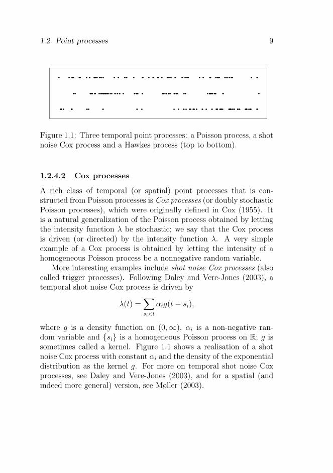
Poisson processes are also used as a reference mark for defining theconcepts of a clustered or regular point process. If the points of a pointpattern tend to fall in clusters more than a Poisson process we saythat the point pattern is clustered. Conversely, if the points insteadtend to be more evenly distributed than a Poisson process, we saythat it is regular. Figure 1.1 shows a realisation of a temporal Poissonprocess. Furthermore, two clustered point processes are shown; theseprocesses are introduced in Sections 1.2.4.2 and 1.2.4.3. From thefigure it is clear that the events of the two clustered processes tendmore to fall in clusters than the events of the Poisson process.
Poisson processes are a huge subject, and e.g. Kingman (1993) isdedicated to the study of these. Furthermore, many books on pointprocesses have a chapter on Poisson processes, see e.g. Møller andWaagepetersen (2004) or Daley and Vere-Jones (2003).
1.2. Point processes 9
Figure 1.1: Three temporal point processes: a Poisson process, a shotnoise Cox process and a Hawkes process (top to bottom).
1.2.4.2 Cox processes
A rich class of temporal (or spatial) point processes that is con-structed from Poisson processes is Cox processes (or doubly stochasticPoisson processes), which were originally defined in Cox (1955). Itis a natural generalization of the Poisson process obtained by lettingthe intensity function λ be stochastic; we say that the Cox processis driven (or directed) by the intensity function λ. A very simpleexample of a Cox process is obtained by letting the intensity of ahomogeneous Poisson process be a nonnegative random variable.
More interesting examples include shot noise Cox processes (alsocalled trigger processes). Following Daley and Vere-Jones (2003), atemporal shot noise Cox process is driven by
λ(t) =∑
si<t
αig(t− si),
where g is a density function on (0,∞), αi is a non-negative ran-dom variable and {si} is a homogeneous Poisson process on R; g issometimes called a kernel. Figure 1.1 shows a realisation of a shotnoise Cox process with constant αi and the density of the exponentialdistribution as the kernel g. For more on temporal shot noise Coxprocesses, see Daley and Vere-Jones (2003), and for a spatial (andindeed more general) version, see Møller (2003).
10 Chapter 1. Introduction
Another interesting example is log Gaussian Cox processes. Thelog Gaussian Cox processes are defined by their intensity, which is theexponential of a Gaussian field. The theory of log Gaussian processescan be found in Møller et al. (1998).
1.2.4.3 Cluster processes
A cluster process is a point process intended for modelling clusteredpoint patterns by constructing clusters individually. The definitionof a cluster process is divided into two parts. Firstly a point processknown as a centre process is generated. Then each point (or centre) inthe centre process generates a new point process called a componentprocess or a cluster. The cluster process consists of the superpositionof the clusters, where the centres may or may not be included. Thecentres are also sometimes called ancestors, parents or immigrants,the points in the clusters are sometimes called children or offspring,and if the centres follow a Poisson process, the cluster process is calleda Poisson cluster process.
An example of a Poisson cluster process is the Thomas process(Thomas, 1949). Here the clusters are i.i.d. relative to their centresand each cluster is itself a Poisson process where the intensity func-tion is proportional to the normal density function with the clustercentre as mean and some fixed variance. Another example is the shotnoise Cox process described in Section 1.2.4.2.
An example of a Poisson cluster process where the clusters arenot simply Poisson processes is the Hawkes process (or self-excitingprocess). There are two equivalent ways of defining the Hawkes pro-cess. The first way is by specifying its conditional intensity function;for example, in the unmarked case, this is given by
λ(t) = µ(t) +∑
ti<t
γ(t− ti),
where µ and γ are non-negative, measurable functions and γ(t) = 0for t ≤ 0. The conditional intensity function (or, more precisely,
1.3. Lattice processes 11
the ground intensity) for the marked case is given by formula (2.1)in Chapter 2. The other way is to use a construction of clusterswith a certain branching structure of Poisson processes; this is donein Definition 2.1 in Chapter 2. Figure 1.1 shows a realisation ofan unmarked Hawkes process, where γ is an exponentially decayingfunction on [0,∞), and µ is constant. Since the Hawkes process isthe focus of Chapters 2 and 3, I will postpone all further details untilthese chapters. For more theory on Hawkes processes, see Hawkes(1971a,b, 1972); Hawkes and Oakes (1974); Bremaud and Massoulie(2001, 2002); Torrisi (2002), and for applications of Hawkes processes,see e.g. Vere-Jones and Ozaki (1982); Chornoboy et al. (1988); Ogata(1988, 1998). A purely spatial version of this process also exists, seeMøller and Torrisi (2005).
1.3 Lattice processes
1.3.1 Definition
A lattice process (or lattice model) is used to model a system of ran-dom variables associated to a set of sites, where sites for examplecould represent a fixed set of physical locations or times. Basically,a lattice process is just a random vector X, where each entry in thevector xi correspond to a site i. Thus we could define a lattice processby its joint distribution. However, as Besag (1974) points out, it isusually more convenient to specify a lattice process by the conditionaldistribution Pi of the random variable xi at a site i given the set of allother sites. In Chapter 4 we refer to this as the local characteristicsince it describes the local behaviour of the process. Note that Pi
has much the same role as the conditional intensity defined for tem-poral processes in Section 1.2.2. Much like the conditional intensity,it provides an easy way of defining a model on a complex systemby defining what is happening locally. However, it does not havethe evolutionary character which makes the conditional intensity souseful.
12 Chapter 1. Introduction
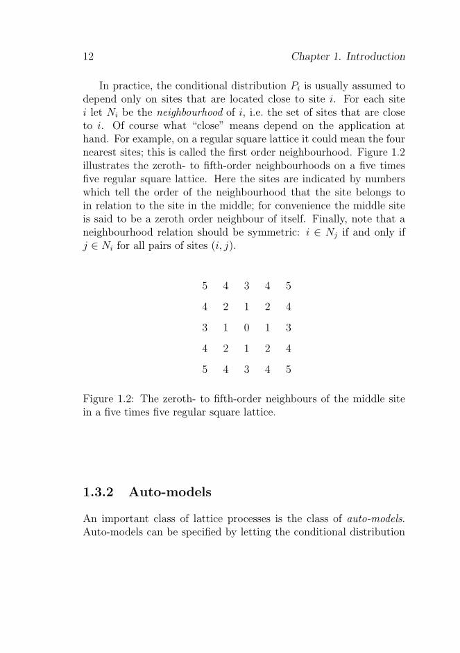
In practice, the conditional distribution Pi is usually assumed todepend only on sites that are located close to site i. For each sitei let Ni be the neighbourhood of i, i.e. the set of sites that are closeto i. Of course what “close” means depend on the application athand. For example, on a regular square lattice it could mean the fournearest sites; this is called the first order neighbourhood. Figure 1.2illustrates the zeroth- to fifth-order neighbourhoods on a five timesfive regular square lattice. Here the sites are indicated by numberswhich tell the order of the neighbourhood that the site belongs toin relation to the site in the middle; for convenience the middle siteis said to be a zeroth order neighbour of itself. Finally, note that aneighbourhood relation should be symmetric: i ∈ Nj if and only ifj ∈ Ni for all pairs of sites (i, j).
5
4
3
4
5
4
2
1
2
4
3
1
0
1
3
4
2
1
2
4
5
4
3
4
5
Figure 1.2: The zeroth- to fifth-order neighbours of the middle sitein a five times five regular square lattice.
1.3.2 Auto-models
An important class of lattice processes is the class of auto-models.Auto-models can be specified by letting the conditional distribution

1.3. Lattice processes 13
of a site i given its neighbours Pi(xi|Ni) have the form
Pi(xi|Ni) ∝ exp
(
xiGi(xi) +∑
j∈Ni
βi,jxixj
)
,
where Gi is a real-valued function and βi,j ∈ R fulfills that βi,j = βj,i
for each pair of sites (i, j).One example of an auto-model is the autologistic model. For each
site i, let xi be Bernoulli distributed and Gi(xi) = αi be constant.The autologistic model can then be specified through its conditionaldistribution at site i,
Pi(xi|Ni) =exp(αixi +
∑
j∈Niβi,jxixj)
1 + exp(αi +∑
j∈Niβi,jxj)
.
Locally βi,j is easily interpreted: a positive βi,j means that xi willtend to have the same value as xj, whereas a negative βi,j means itwill tend to have a different value than xj. Globally an autologisticmodel with numerically large, positive values for βi,j has large clustersof zeros and ones. In the case of a first order neighbourhood on asquare lattice, an autologistic model with numerically large, negativevalues for βi,j tends to have chess board patterns. These two casesof patterns of zeros and ones are analogous to clustered and regularpoint patterns. The size of the parameter space is usually reduced forthis model to be practically useful, for example by setting βi,j = β forall neighbour pairs (i, j) and αi = α for all i. Figure 1.3 shows tworealisations of autologistic processes with a first order neighbourhoodon a 20 × 20 lattice; on the left-hand side β is positive, and on theright-hand side β is negative.
One problem associated with the autologistic model is that thelikelihood function is known only up to an unknown normalizing con-stant; by the Hammersley-Clifford theorem (see e.g. Besag (1974)),the likelihood function can be shown to be
L =1
cexp
(
∑
i
αixi +∑
i
∑
j∈Ni,j>i
βi,jxixj
)
,

14 Chapter 1. Introduction
Figure 1.3: Left: a realisation of the autologistic model with positiveβi,j = β. Right: as left, but with negative βi,j = β.
where c denotes the normalizing constant. It is only feasible to calcu-late the normalizing constant through brute force in cases with smalllattices. Otherwise techniques such as those mentioned at the end ofSection 1.2.2 are needed.
There are of course many other auto-models than the autologisticmodel, for example the auto-Poisson model, where the conditionaldistribution of xi is Poisson. For details on this and other auto-models, see Besag (1974).
1.4 Simulation
Most point processes of any applicational value are quite complexstochastic processes, and often it is impossible to derive quantities ofinterest analytically. Instead one must turn to simulation algorithmsfor approximating such quantities. Simulation is an invaluable toolfor example in parameter estimation, model checking, and prediction.Even something as simple as getting an idea of what a typical reali-sation of a particular type of point process looks like may require theuse of a simulation algorithm.
There are many different simulation algorithms available for sim-ulating a point process with a given set of parameters; many of these
1.4. Simulation 15
algorithms are tailored to specific classes of point processes, whileothers are rather general but not always very efficient. I will in noway try to give a comprehensive introduction to the subject; insteadI will focus on algorithms that are relevant to the later chapters.
1.4.1 Poisson and related processes
Since the Poisson process is one of the simplest examples of pointprocesses, it is probably not much of a surprise that it is also one ofthe simplest processes to simulate. The homogeneous temporal Pois-son process with intensity λ is easily simulated on an interval [0, t+)by using that the lengths of the time intervals between subsequentevents are i.i.d. exponentially distributed random variables. Firstsimulate i.i.d. exponential variables Yi with inverse mean λ. Eachevent are then given by ti =
∑i
j=1 Yj. The algorithm terminatesonce the end of the time interval t+ has been reached. Another wayof simulating a homogeneous Poisson process with intensity λ is asfollows: first simulate the number of events as a Poisson variable withmean λt+ and then simulate the times of the events as i.i.d. uniformvariables on [0, t+). This latter method generalizes directly to thespatial Poisson process, where we need to simulate uniform variableson the simulation region.
Inhomogeneous Poisson processes can be simulated in several waysdepending on the shape of the intensity function. A quite general wayis independent thinning. Independent thinning means that we takea point process X1 = {ti} and obtain another process X2 by inde-pendently keeping each event ti from X1 with a specified probabilityp(ti) (called the retention probability), or otherwise throw ti away.If X1 is a Poisson process with intensity function λ1(t), then X2 is aPoisson process with intensity λ2(t) = p(t)λ1(t) (see e.g. Møller andWaagepetersen (2004)). This means we can simulate an inhomoge-neous Poisson process X2 with a bounded intensity λ2(t) by usingindependent thinning on a simulation of a homogeneous Poisson pro-cess X1 with intensity λ1 = sup(λ2(t)). For specific functional forms
16 Chapter 1. Introduction
of the intensity function, it may be more convenient to use otheralgorithms. For example, if the intensity has the shape of an unnor-malized exponential density function, then it is easiest to simulate itby first simulating the number of events as the appropriate Poissonvariable, and then simulate the time of each event as i.i.d. exponentialvariables.
Since many processes are defined using the Poisson process asa starting point, it is often possible to simulate these directly byexploiting the definition. For example, conditionally on the intensity,a Cox process is a Poisson process, so if we can simulate the intensity,then we can simply simulate the Poisson process afterwards using oneof the above techniques. Another example is the Hawkes process. Ifthe Hawkes process is defined using Poisson processes as in Chapter 3,then Algorithm 3.1 is an straightforward procedure for simulatingthe process once one knows a simulation algorithm for the Poissonprocesses used in the definition.
1.4.2 Simulation using the conditional intensity
One of the reasons that the conditional intensity function is so use-ful is that it leads to two rather general simulation algorithms forevolutionary temporal point processes.
One of these algorithms is Ogata’s modified thinning algorithm(Ogata, 1981), or rather, its generalization to marked processes (seee.g. Daley and Vere-Jones (2003), page 273). This algorithm is ageneralization of the independent thinning algorithm used for simu-lating inhomogeneous Poisson processes as described in Section 1.4.1.The basic idea behind Ogata’s modified thinning algorithm is thatwe start at the first time in the simulation interval (e.g. time 0 inthe interval [0, t+)) and go forward in time. We propose new eventsone after another, and check right away whether to keep an event,since this changes the conditional intensity function for later times.More specifically, the algorithm requires that there exists two func-tions m(t) = m(t|Ht−) and l(t) = l(t|Ht−) such that λg(t+u) ≤ m(t)
1.4. Simulation 17
for 0 ≤ u < l(t). The function l(t) is the maximum length of time wewill go forward in time in one step of the algorithm, and m(t) is themaximum value that the conditional intensity may attain in this in-terval. For simulating a process on the interval [0, t+), the algorithmfor the marked case is as follows:
Algorithm 1.1 (Ogata’s modified thinning algorithm.)
1. Set t=0 and n=0.
2. Repeat until t > t+:
(a) Compute m(t) and l(t).
(b) Generate independent random variables T ∼ Exp(m(t))and U ∼ Unif([0, 1]).
(c) If T > l(t), set t = t+ l(t).
(d) Else if t+ T > t+ or U > λg(t+ T )/m(t), set t = t+ T .
(e) Otherwise, set n = n+1, tn = t+T , t = t+T and simulatezn ∼ Q.
3. Output is {t1, . . . , tn}.
Here Exp(m(t)) denotes the exponential distribution with inversemean m(t), and Unif([0, 1]) denotes the uniform distribution on theinterval [0, 1]. This algorithm is very useful for simulating the pointprocess used in Chapter 5, but it is much less efficient than Algo-rithm 3.1 in Chapter 3 for simulating Hawkes processes.
The other algorithm that uses the conditional intensity functionfor simulating evolutionary temporal point processes is simulation byinversion. The basic idea in this algorithm is that we simulate anumber of unit exponential variables, and then we transform theseinto time intervals for the process we are simulating. Assuming thatwe want to simulate the process on [0, t+), the algorithm is as follows:
18 Chapter 1. Introduction
Algorithm 1.2 (Simulation by inversion.)
1. Set t = 0, t0 = 0 and n = 0 (note that t0 is not an event).
2. Repeat until t > t+:
(a) Generate T ∼ Exp(1).
(b) Calculate t, where T =∫ t
tnλ(s)ds.
(c) If t < t+, set n = n+ 1 and tn = t.
3. Output is {t1, . . . , tn}.
The difficult part of this algorithm is of course calculating t in step(2b) since this requires finding the inverse of the integrated condi-tional intensity function.
1.4.3 Simulation using MCMC
It often happens that a stochastic process is too complex to simu-late directly, but when all else fails, one can usually turn to Markovchain Monte Carlo (MCMC) techniques for simulating a point pro-cess. Spatial point processes and spatial lattice processes are twotypes of stochastic processes that frequently require the use of anMCMC algorithm for simulation. Furthermore, inference for mostpoint processes or lattice processes is often not possible analytically.Instead MCMC based simulation is useful for obtaining, for exam-ple, an approximation of the posterior distributions of parameters inthe case of Bayesian inference (for an introduction to Bayesian infer-ence, see e.g. Gelman et al. (2004)). I will assume that the conceptsof MCMC is well-known to the reader; for an introduction to Mar-kov chains, see e.g. Meyn and Tweedie (1993) or Norris (1997), andfor an introduction to MCMC in practice with a focus on posteriordistributions, see Tierney (1994).
Since we never meet any point process that requires the use ofan MCMC algorithm for simulation in this thesis, I will not go
1.5. Missing data 19
into details with simulation algorithms for these; see e.g. Møller andWaagepetersen (2004) or van Lieshout (2000) for introductions tothis subject. Instead I will consider the following algorithm for sim-ulating a lattice process, since this is used in Chapter 4. We start atsome configuration (say all xi = 0) and use a Gibbs sampler wherewe update each xi one at a time in some random or fixed order.Each xi is updated by drawing a new value for xi from it conditionaldistribution given the state of all the other sites Pi.
One of the problems with MCMC based approaches is that inprinciple the Markov chains have to run infinitely long before reach-ing the target distribution. One solution to this problem is to putthe MCMC algorithm into the framework of perfect simulation. Byperfect simulation is meant that the output of the algorithm followsthe target distribution exactly. In Chapter 4, the Gibbs sampler de-scribed above is combined with a perfect simulation technique knownas Propp-Wilson’s coupling from the past (Propp and Wilson, 1996)to obtain perfect simulations. Other examples of perfect simulationinclude dominated coupling from the past (Kendall and Møller, 2000),Wilson’s read-once algorithm (Wilson, 2000), and perfect simulationusing clans of ancestors (Fernandez et al., 2002). For an overview ofvarious perfect simulation algorithms in relation to point processes,see Møller and Waagepetersen (2004).
1.5 Missing data
Often it is the case that a useful model needs more information thanthe observed data provides. That is, we have a so-called missing dataproblem. In this thesis, missing data in various forms are centralparts of the problems studied, and therefore I will introduce the twomissing data problems which will be treated in Chapters 2–5.
20 Chapter 1. Introduction
1.5.1 Edge effects
Many point processes are defined on an infinite set, e.g. the timeline R, but in practice we only observe data on a finite observationregion. However, the observed data may depend on the unobserveddata outside the observation region. If we try to simulate new dataon the observation region without taking this fact into account, thenthe simulation will not be exact. Furthermore, calculations of variousfunctions, such as the likelihood function, may also contain errors.The errors resulting from only observing the process on a limitedregion without taking the region outside the observation region intoaccount are known as edge effects. Many kinds of stochastic processessuffer from edge effects, but I will only consider point processes, andfurthermore I will focus on edge effects in relation to simulation.
Evolutionary temporal point processes are usually simulated on atime interval, say [0, t+), but what happens during this time intervalmay depend on the past. For example, we may wish to simulate atemporal point process model for the times of earthquakes and theiraftershocks aftershocks. If we simply simulate the times of earth-quakes and aftershocks on [0, t+) and completely ignore that theremay have been earthquakes before time 0, then the aftershocks ofearthquakes occurring before time 0 will be missing. Results basedon such a simulation will be biased and may lead to the wrong con-clusions. Since simulation is an important tool for prediction andmodel checking for point processes, methods are needed for dealingwith edge effects.
An easy, but only approximate, method for simulating a pointprocess without edge effects is to simulate it on a larger region. Inthe case of an evolutionary temporal point process on [0, t+), thismeans that we would start our simulation at some time before time0, say t− < 0; the question is what value of t− we should choose toobtain a simulation without significant edge effects. Algorithm 3.1in Chapter 3 simulates a Hawkes process by starting at time t−. Inthat chapter, various ways of quantifying edge effects are considered
1.5. Missing data 21
to obtain an idea of what t− to choose to make a simulation withinsignificant edge effects (see also Bremaud and Massoulie (2002) andBremaud et al. (2002)). In principle, most simulation algorithms,for example Ogata’s modified thinning algorithm, can be used on alarger region, but in general it is difficult to determine how large thesimulation region should be.
There are also algorithms which can simulate specific classes ofpoint processes completely without edge effects. Brix and Kendall(2002) (see also Møller (2003)) introduces a clever way of simulatingpoint processes that are simultaneously Poisson cluster processes andCox processes without any edge effects. They simulate exactly thoseclusters which have one or more events inside the simulation region,whether or not the cluster centre is inside the simulation region. InChapter 2 we make a non-trivial extension to this simulation methodand obtain a simulation algorithm for the Hawkes process that doesnot suffer from edge effects.
There are many other methods for dealing with edge effects invarious contexts. Møller and Waagepetersen (2004), Daley and Vere-Jones (2003), and some of the references therein provide various tech-niques of dealing with edge effects in simulations and calculations, e.g.minus sampling, edge correction factors, and periodic boundaries.
1.5.2 Continuous time processes observed at dis-
crete times
Stochastic processes may be defined on a continuous subset of thetime line R, but sometimes it may only be possible to observe theprocess on a discrete set of observation times. For example, an eventmay be that a tree has become infested with insects, but in orderto detect the time of this event, we will need to observe the treecontinuously, which may not possible in practice. If the data is onlyobserved at discrete times, it only provides partial information aboutthe events, for example whether or not one or more events have oc-curred between two observation times. Obviously, such a missing
22 Chapter 1. Introduction
data setup of discrete observation times can apply to many types ofcontinuous time stochastic processes, but in this thesis the attentionwill be restricted to multivariate temporal point processes.
There are several ways of dealing with this missing data prob-lem for a multivariate temporal point process. One way is simplyto ignore that the observed and unobserved data are continuous andinstead model only the observed data using a discrete time process,i.e. a lattice process can be used instead of a multivariate temporalpoint process. This seems to be the standard approach for modellingsuch systems, and has for example been done in Besag and Tantrum(2003). However, this approach is not unproblematic. In Chapter 4, acomplex system of trees and insects with annual observations is mod-elled using a spatio-temporal autoregressive type of model. However,in this particular model unknown normalising constants appear inthe likelihood function, which complicates the computations consid-erably.
Another way is to specify a continuous time model and then sim-ulate the missing data using MCMC. In general, this approach mayseem to be conceptually and computationally more difficult than thediscrete time approach, and this approach seems to be avoided in theliterature. However, in some cases the inclusion of continuous timemay pay off. In Chapter 5, a part of the discretely observed data fromChapter 4 is modelled using a multivariate temporal point process.There the inclusion of continuous time means that the conditionalintensity function (see Section 1.2.2) can be used for specifying amodel, which implies that an expression for the likelihood function isavailable without any unknown normalizing constants. In Chapter 5the advantages and disadvantages of the discrete and continuous timeapproaches to the missing data are discussed.
1.5. Missing data 23
References
Besag, J. and Tantrum, J. (2003). Likelihood analysis of binary datain space and time. In P. J. Green, N. L. Hjort, and S. Richard-son, editors, Highly Structured Stochastic Systems, pages 289–295.Oxford University Press, Oxford.
Besag, J. E. (1974). Spatial interaction and the statistical analysis oflattice systems (with discussion). Journal of the Royal StatisticalSociety Series B , 36, 192–236.
Bremaud, P. and Massoulie, L. (2001). Hawkes branching point pro-cesses without ancestors. Journal of Applied Probability , 38, 122–135.
Bremaud, P. and Massoulie, L. (2002). Power spectra of generalshot noises and Hawkes point processes with a random excitation.Advances in Applied Probability , 34, 205–222.
Bremaud, P., Nappo, G., and Torrisi, G. (2002). Rate of convergenceto equilibrium of marked Hawkes processes. Journal of AppliedProbability , 39, 123–136.
Brix, A. and Kendall, W. (2002). Simulation of cluster point processeswithout edge effects. Advances in Applied Probability , 34, 267–280.
Chornoboy, E. S., Schramm, L. P., and Karr, A. F. (1988). Maximumlikelihood identification of neural point process systems. Advancesin Applied Probability , 34, 267–280.
Cox, D. R. (1955). Some statistical models related with series ofevents. Journal of the Royal Statistical Society Series B , 17, 129–164.
Daley, D. J. and Vere-Jones, D. (2003). An Introduction to the Theoryof Point Processes, Volume I: Elementary Theory and Methods .Springer, New York, 2nd edition.
24 Chapter 1. Introduction
Fernandez, R., Ferrari, P. A., and Garcia, N. L. (2002). Perfectsimulation for interacting point processes, loss networks and isingmodels. Stochastic Processes and Their Applications , 102, 63–88.
Gelman, A. and Meng, X. (1998). Simulating normalizing constants:From importance sampling to bridge sampling to path sampling.Statistical Science, 13(2), 163–185.
Gelman, A., Carlin, J. B., Stern, H. S., and Rubin, D. B. (2004).Bayesian Data Analysis . Chapman & Hall, Boca Raton, 2nd edi-tion.
Hawkes, A. G. (1971a). Point spectra of some mutually excitingpoint processes. Journal of the Royal Statistical Society Series B ,33, 438–443.
Hawkes, A. G. (1971b). Spectra of some self-exciting and mutuallyexciting point processes. Biometrika, 58(1), 83–90.
Hawkes, A. G. (1972). Spectra of some mutually exciting point pro-cesses with associated variables. In P. A. W. Lewis, editor, Stochas-tic Point Processes , pages 261–271. Wiley, New York,.
Hawkes, A. G. and Oakes, D. (1974). A cluster representation of aself-exciting process. Journal of Applied Probability , 11, 493–503.
Kendall, W. S. and Møller, J. (2000). Perfect simulation using dom-inating processes on ordered spaces, with application to locallystable point processes. Advances in Applied Probability , 32, 844–865.
Kingman, J. F. C. (1993). Poisson processes . Oxford UniversityPress, Oxford.
Meyn, S. P. and Tweedie, R. L. (1993). Markov Chains and StochasticStability . Springer Verlag, London.
1.5. Missing data 25
Møller, J. (2003). Shot noise Cox processes. Advances in AppliedProbability , 35, 614–640.
Møller, J. and Torrisi, G. L. (2005). Second order analysis for spa-tial hawkes processes. Research Report R-2005-20, Department ofMathematical Sciences, Aalborg University.
Møller, J. and Waagepetersen, R. P. (2004). Statistical Inference andSimulation for Spatial Point Processes . Chapman & Hall, BocaRaton, Florida.
Møller, J., Syversveen, A. R., and Waagepetersen, R. P. (1998). LogGaussian Cox processes. Scandinavian Journal of Statistics , 25,451–482.
Møller, J. M., Pettitt, A. N., Berthelsen, K. K., and Reeves, R. W.(2006). An efficient markov chain monte carlo method for distribu-tions with intractable normalising constants. Biometrika, 93. Toappear.
Norris, J. R. (1997). Markov Chains . Cambridge University Press,New York.
Ogata, Y. (1981). On Lewis’ simulation method for point processes.IEEE Transactions on Information Theory , IT-27(1), 23–31.
Ogata, Y. (1988). Statistical models for earthquake occurrences andresidual analysis for point processes. Journal of the American Sta-tistical Association, 83(401), 9–27.
Ogata, Y. (1998). Space-time point-process models for earthquakeoccurrences. Annals of the Institute of Statistical Mathematics ,50(2), 379–402.
Papangelou, F. (1974). The conditional intensity of general pointprocesses and an application to line processes. Zeitschrift furWahrscheinlichkeitstheorie und Verwandte Gebiete, 28, 207–226.
26 Chapter 1. Introduction
Propp, J. G. and Wilson, D. B. (1996). Exact sampling with coupledMarkov chains and applications to statistical mechanics. RandomStructures and Algorithms, 9, 223–252.
Thomas, M. (1949). A generalization of Poisson’s binomial limit foruse in ecology. Biometrika, 36, 18–25.
Tierney, L. (1994). Markov chains for exploring posterior distribu-tions. The Annals of Statistics , 22(4), 1701–1762.
Torrisi, G. L. (2002). A class of interacting marked point processes:rate of convergence to equilibrium. Journal of Applied Probability ,39, 137–160.
van Lieshout, M. (2000). Markov Point Processes and Their Appli-cations . Imperial College Press, London.
Vere-Jones, D. and Ozaki, T. (1982). Some examples of statisticalinference applied to earthquake data. Annals of the Institute ofStatistical Mathematics , 34, 189–207.
Wilson, D. B. (2000). How to couple from the past using a read-once source of randomness. Random Structures and Algorithms,16, 85–113.
Chapter 2
Perfect simulation of
Hawkes processes
Jesper Møller & Jakob G. Rasmussen
Department of Mathematical Sciences, Aalborg University, FredrikBajers Vej 7G, DK-9220 Aalborg, Denmark.
Email addresses: [email protected] & [email protected]
Abstract
Our objective is to construct a perfect simulation algorithm for un-marked and marked Hawkes processes. The usual straightforwardsimulation algorithm suffers from edge effects, whereas our perfectsimulation algorithm does not. By viewing Hawkes processes as Pois-son cluster processes and using their branching and conditional inde-pendence structures, useful approximations of the distribution func-tion for the length of a cluster are derived. This is used to constructupper and lower processes for the perfect simulation algorithm. Atail-lightness condition turns out to be of importance for the applica-bility of the perfect simulation algorithm. Examples of applicationsand empirical results are presented.
27
28 Chapter 2. Perfect simulation of Hawkes processes
Keywords: Approximate simulation; dominated coupling from thepast; edge effects; exact simulation; marked Hawkes process; markedpoint process; perfect simulation; point process; Poisson cluster pro-cess; thinning; upper process; lower process
2000 Mathematical Subject Classification: Primary 60G55Secondary 68U20
2.1 Introduction
Unmarked and marked Hawkes processes (Hawkes, 1971a,b, 1972;Hawkes and Oakes, 1974) play a fundamental role for point pro-cess theory and its applications, cf., for example, Daley and Vere-Jones (2003), and they have important applications in seismology(Hawkes and Adamopoulos, 1973; Ogata, 1988, 1998; Vere-Jones andOzaki, 1982) and neurophysiology (Bremaud and Massoulie, 1996;Chornoboy et al., 2002). There are many ways to define a markedHawkes process, but for our purpose it is most convenient to defineit as a marked Poisson cluster process X = {(ti, Zi)} with events (ortimes) ti ∈ R and marks Zi defined on an arbitrary (mark) space Mequipped with a probability distribution Q. The cluster centres of Xare given by certain events called immigrants, while the other eventsare called offspring.
Definition 2.1 (Hawkes process with unpredictable marks.)
(a) The immigrants follow a Poisson process with a locally inte-grable intensity function µ(t), t ∈ R.
(b) The marks associated to the immigrants are independent andidentically distributed (i.i.d.) with distribution Q, and are in-dependent of the immigrants.
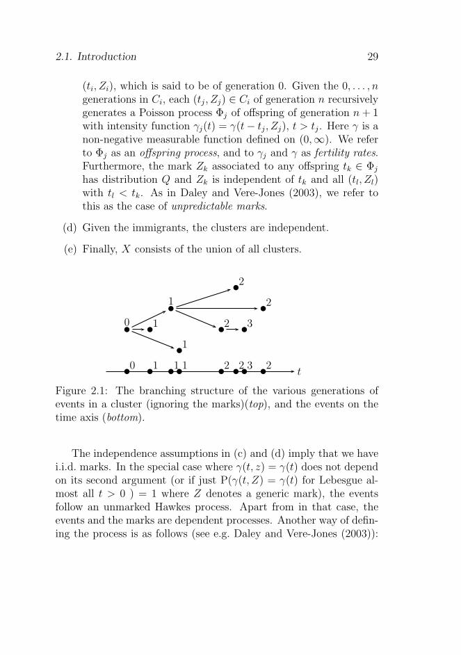
(c) Each immigrant ti generates a cluster Ci, which consists ofmarked events of generations of order n = 0, 1, . . . with thefollowing branching structure (see Figure 2.1). We first have
2.1. Introduction 29
(ti, Zi), which is said to be of generation 0. Given the 0, . . . , ngenerations in Ci, each (tj, Zj) ∈ Ci of generation n recursivelygenerates a Poisson process Φj of offspring of generation n+ 1with intensity function γj(t) = γ(t− tj, Zj), t > tj. Here γ is anon-negative measurable function defined on (0,∞). We referto Φj as an offspring process, and to γj and γ as fertility rates.Furthermore, the mark Zk associated to any offspring tk ∈ Φj
has distribution Q and Zk is independent of tk and all (tl, Zl)with tl < tk. As in Daley and Vere-Jones (2003), we refer tothis as the case of unpredictable marks.
(d) Given the immigrants, the clusters are independent.
(e) Finally, X consists of the union of all clusters.
0
1
1
1
2
2
2 3
0 11 1 2 22 3t
Figure 2.1: The branching structure of the various generations ofevents in a cluster (ignoring the marks)(top), and the events on thetime axis (bottom).
The independence assumptions in (c) and (d) imply that we havei.i.d. marks. In the special case where γ(t, z) = γ(t) does not dependon its second argument (or if just P(γ(t, Z) = γ(t) for Lebesgue al-most all t > 0 ) = 1 where Z denotes a generic mark), the eventsfollow an unmarked Hawkes process. Apart from in that case, theevents and the marks are dependent processes. Another way of defin-ing the process is as follows (see e.g. Daley and Vere-Jones (2003)):

30 Chapter 2. Perfect simulation of Hawkes processes
The marks are i.i.d. and the conditional intensity function λ(t) at timet ∈ R for the events given the previous history {(tk, Zk) : tk < t} isgiven by
λ(t) = µ(t) +∑
ti<t
γ(t− ti, Zi). (2.1)
Simulation procedures for Hawkes processes are needed for vari-ous reasons: Analytical results are rather limited due to the complexstochastic structure; statistical inference, especially model checkingand prediction, require simulations; and displaying simulated realiza-tions of specific model constructions provides a better understandingof the model. The general approach for simulating a (marked orunmarked) point process is to use a thinning algorithm such as theShedler-Lewis thinning algorithm or Ogata’s modified thinning algo-rithm (see e.g. Daley and Vere-Jones (2003)). However, Definition 2.1immediately leads to the following approximate simulation algorithm,where t− ∈ [−∞, 0] and t+ ∈ (0,∞] are user-specified parameters,and the output consists of all marked points (ti, Zi) with ti ∈ [0, t+).
Algorithm 2.1 The following steps (i)-(ii) generate an approximatesimulation of those marked events (ti, Zi) ∈ X with 0 ≤ ti < t+.
(i) Simulate the immigrants on [t−, t+).
(ii) For each such immigrant ti, simulate Zi and those (tj, Zj) ∈ Ci
with ti < tj < t+.
In general Algorithm 2.1 suffers from edge effects, since clustersgenerated by immigrants before time t− may contain offspring in[0, t+). Bremaud et al. (2002) studied the ‘rate of installation’, i.e.they considered a coupling of X, after time 0, with the output fromAlgorithm 2.1 when t+ = ∞. Under a tail-lightness assumption (seethe paragraph after Proposition 2.3, below) and other conditions,they established an exponentially decreasing bound for the probabil-ity P(t−,∞), say, that X, after time 0, coincides with the output ofthe algorithm. Algorithm 2.1 is also investigated in our own work
2.1. Introduction 31
(Møller and Rasmussen, 2004) where various measures for edge ef-fects, including refined results for P(t−,∞), were introduced.
Our objective in this paper is to construct a perfect (or exact) sim-ulation algorithm. Perfect simulation has been a hot research topicsince the seminal Propp-Wilson algorithm (Propp and Wilson, 1996)appeared, but the areas of application have so far been rather limitedand many perfect simulation algorithms proposed in the literature aretoo slow for real applications. As demonstrated in Møller and Ras-mussen (2004) our perfect simulation algorithm can be practical andefficient. Moreover, apart from the advantage of not suffering fromedge effects, our perfect simulation algorithm can also be useful inquantifying the edge effects suffered by Algorithm 2.1 (see Møller andRasmussen (2004)).
The perfect simulation algorithm is derived using similar princi-ples as in Brix and Kendall (2002), but our algorithm is a non-trivialextension, since the Brix-Kendall algorithm requires the knowledgeof the cumulative distribution function (CDF) F for the length of acluster, and F is unknown even for the simplest examples of Hawkesprocesses. By establishing certain monotonicity and convergence re-sults, we are able to approximate F to any required precision, and,more importantly, to construct a dominating process and upper andlower processes in a similar fashion as in the dominated-coupling-from-the-past algorithm of Kendall and Møller (2000). Under a tail-lightness condition, our perfect simulation algorithm turns out to befeasible in applications, while in the heavy-tailed case, we can at leastsay something about the approximate form of F , cf. Example 2.7.
The paper is organised as follows. Section 2.2 contains some pre-liminaries, including illuminating examples of Hawkes process modelsused throughout the paper to illustrate our results. In Section 2.3, wedescribe the perfect simulation algorithm, assuming that F is known,while the above-mentioned convergence and monotonicity results areestablished in Section 2.4. Section 2.5 completes the perfect simu-lation algorithm, using dominated coupling from the past. Finally,Section 2.6 contains a discussion of our algorithm and results, and
32 Chapter 2. Perfect simulation of Hawkes processes
suggestions on how to extend these to more general settings.
2.2 Preliminaries and examples
2.2.1 The branching structure and self-similarity
property of clusters
By Definition 2.1, we can view the marked Hawkes process X ={(ti, Zi)} as a Poisson cluster process with cluster centres given by theimmigrants, where the clusters, given the immigrants, are indepen-dent. In this section, we describe a self-similarity property resultingfrom the specific branching structure within a cluster.
For events ti < tj, we say that (tj, Zj) has ancestor ti of ordern ≥ 1 if there is a sequence s1 . . . , sn of offspring such that sn = tjand sk, k = 1, . . . , n, is one of the offspring of sk−1, with s0 = ti. Wethen say that tj is an offspring of nth generation with respect to ti;for convenience, we say that ti is of zeroth generation with respect toitself. Now we define the total offspring process Ci as all those (tj, Zj)such that tj is an event of generation n ∈ N0 with respect to ti (notethat (ti, Zi) ∈ Ci). The clusters are defined as those Ci for which tiis an immigrant (see Definition 2.1).
The total offspring processes have the same branching structurerelative to their generating events. More precisely, since γi(t) = γ(t−ti, Zi) for any event ti, we see by Definition 2.1 that conditional onevents ti < tj, the translated total offspring processes Ci − ti ≡{(tl − ti, Zl) : (tl, Zl) ∈ Ci} and Cj − tj ≡ {(tl − tj, Zl) : (tl, Zl) ∈ Cj}are identically distributed.
In particular, conditional on the immigrants, the clusters relativeto their cluster centres (the immigrants) are i.i.d. with distributionP, say. Furthermore, conditional on a cluster’s nth generation eventsGn, say, in a cluster, the translated total offspring processes Cj − tjwith tj ∈ Gn are i.i.d. with distribution P. We refer to this lastproperty as the i.i.d. self-similarity property of offspring processes or,
2.2. Preliminaries and examples 33
for short, the self-similarity property. Note that the assumption ofunpredictable marks is essential for these properties to hold.
2.2.2 A basic assumption and some terminology
and notation
Let F denote the CDF for the length L of a cluster, i.e. the timebetween the immigrant and the last event of the cluster. Considerthe mean number of events in any offspring process Φ(ti), ν ≡ Eν,where
ν =
∫ ∞
0
γ(t, Z) dt
is the total fertility rate of an offspring process and Z denotes ageneric mark with distribution Q. Henceforth, we assume that
0 < ν < 1. (2.2)
The condition ν < 1 appears commonly in the literature on Haw-kes processes (see e.g. Bremaud et al. (2002), Daley and Vere-Jones(2003), and Hawkes and Oakes (1974)), and is essential to our con-vergence results in Section 2.4.2. It implies that
F (0) = Ee−ν > 0 (2.3)
where F (0) is the probability that a cluster has no offspring. It isequivalent to assuming that ES < ∞, where S denotes the numberof events in a cluster: by induction on n = 0, 1 . . ., because of thebranching and conditional independence structure of a cluster, νn isthe mean number of generation n events in a cluster, meaning that
ES = 1 + ν + ν2 + · · · = 1/(1 − ν) (2.4)
if ν < 1, while ES = ∞ otherwise.The other condition, ν > 0, excludes the trivial case where there
are almost surely no offspring. It is readily seen to be equivalent to
F < 1. (2.5)
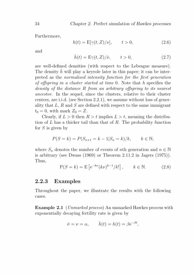
34 Chapter 2. Perfect simulation of Hawkes processes
Furthermore,
h(t) = E[γ(t, Z)/ν], t > 0, (2.6)
and
h(t) = Eγ(t, Z)/ν, t > 0, (2.7)
are well-defined densities (with respect to the Lebesgue measure).The density h will play a keyrole later in this paper; it can be inter-preted as the normalised intensity function for the first generationof offspring in a cluster started at time 0. Note that h specifies thedensity of the distance R from an arbitrary offspring to its nearestancestor. In the sequel, since the clusters, relative to their clustercenters, are i.i.d. (see Section 2.2.1), we assume without loss of gener-ality that L, R and S are defined with respect to the same immigrantt0 = 0, with mark Z0 = Z.
Clearly, if L > 0 then R > t implies L > t, meaning the distribu-tion of L has a thicker tail than that of R. The probability functionfor S is given by
P (S = k) = P (Sn+1 = k − 1|Sn = k)/k, k ∈ N,
where Sn denotes the number of events of nth generation and n ∈ N
is arbitrary (see Dwass (1969) or Theorem 2.11.2 in Jagers (1975)).Thus,
P(S = k) = E[
e−kν(kν)k−1/k!]
, k ∈ N. (2.8)
2.2.3 Examples
Throughout the paper, we illustrate the results with the followingcases.
Example 2.1 (Unmarked process) An unmarked Hawkes process withexponentially decaying fertility rate is given by
ν = ν = α, h(t) = h(t) = βe−βt,

2.2. Preliminaries and examples 35
where 0 < α < 1 and β > 0 are parameters. Here 1/β is a scaleparameter for both the distribution of R and the distribution of L.
The left-hand panel of Figure 2.2 shows perfect simulations ofthis process on [0, 10] when µ(t) = 1 is constant, α = 0.9, and β =10, 5, 2, 1. By (2.4), we expect to see about 10 clusters (in total) and100 events. The clusters of course become more visible as β increases.
The left-hand panel of Figure 2.3 shows six simulations of clusterswith α = 0.9. Here, α is an inverse scaling parameter; β is irrelevantsince, to obtain comparable results for this example and the followingtwo examples, we have omitted showing the scale. All the clustershave been simulated conditional on S > 1 to avoid the frequent andrather uninteresting case containing only the immigrant. These fewsimulations indicate the general tendency of L vary widely. 2
Example 2.2 (Birth-death process) Consider a marked Hawkes pro-cess with
γ(t, Z) = α1(t ≤ Z)/EZ,
where α, 0 < α < 1, is a parameter, Z is a positive random variable,and 1(·) denotes the indicator function. Then X can be viewed as abirth-death process with birth at time ti and survival time Zi of thei’th individual. The birth rate is
λ(t) = µ(t) + (α/EZ)card(
{i : ti < t ≤ ti + Zi})
, t ∈ R,
(cf. (2.1)). Moreover,
ν = αZ/EZ, ν = α, h(t) = E(1(t ≤ Z)/Z), h(t) = P(Z ≥ t)/EZ.
Since ν is random, the distribution of S is more dispersed than in theunmarked case (cf. (2.8)).
The special case where µ(t) = µ is constant and Z is exponentiallydistributed with mean 1/β is considered at page 136 in Bremaudet al. (2002). In this case, X is a time-homogeneous Markov birth-death process with birth rate µ + αβn and death rate βn, where
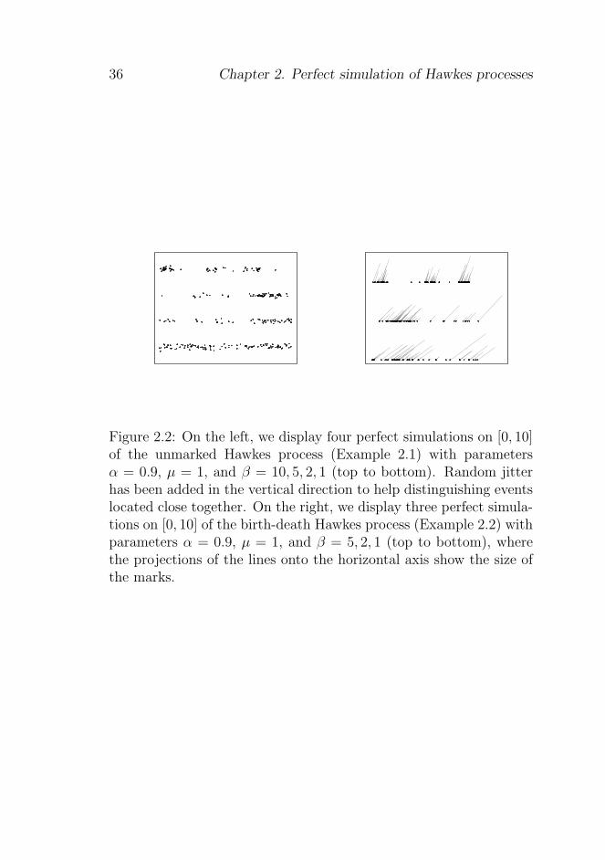
36 Chapter 2. Perfect simulation of Hawkes processes
Figure 2.2: On the left, we display four perfect simulations on [0, 10]of the unmarked Hawkes process (Example 2.1) with parametersα = 0.9, µ = 1, and β = 10, 5, 2, 1 (top to bottom). Random jitterhas been added in the vertical direction to help distinguishing eventslocated close together. On the right, we display three perfect simula-tions on [0, 10] of the birth-death Hawkes process (Example 2.2) withparameters α = 0.9, µ = 1, and β = 5, 2, 1 (top to bottom), wherethe projections of the lines onto the horizontal axis show the size ofthe marks.
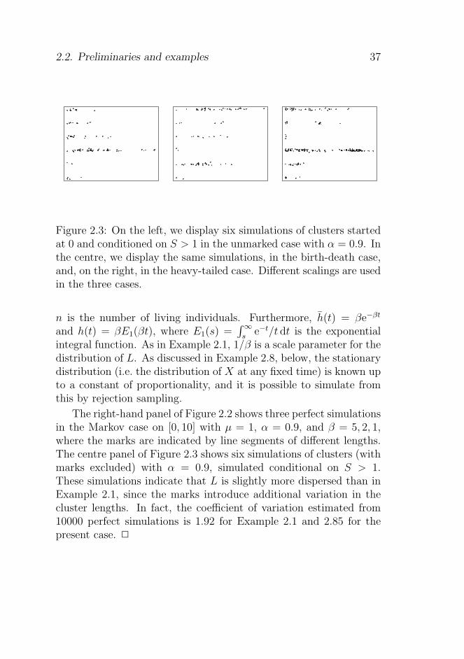
2.2. Preliminaries and examples 37
Figure 2.3: On the left, we display six simulations of clusters startedat 0 and conditioned on S > 1 in the unmarked case with α = 0.9. Inthe centre, we display the same simulations, in the birth-death case,and, on the right, in the heavy-tailed case. Different scalings are usedin the three cases.
n is the number of living individuals. Furthermore, h(t) = βe−βt
and h(t) = βE1(βt), where E1(s) =∫∞
se−t/t dt is the exponential
integral function. As in Example 2.1, 1/β is a scale parameter for thedistribution of L. As discussed in Example 2.8, below, the stationarydistribution (i.e. the distribution of X at any fixed time) is known upto a constant of proportionality, and it is possible to simulate fromthis by rejection sampling.
The right-hand panel of Figure 2.2 shows three perfect simulationsin the Markov case on [0, 10] with µ = 1, α = 0.9, and β = 5, 2, 1,where the marks are indicated by line segments of different lengths.The centre panel of Figure 2.3 shows six simulations of clusters (withmarks excluded) with α = 0.9, simulated conditional on S > 1.These simulations indicate that L is slightly more dispersed than inExample 2.1, since the marks introduce additional variation in thecluster lengths. In fact, the coefficient of variation estimated from10000 perfect simulations is 1.92 for Example 2.1 and 2.85 for thepresent case. 2
38 Chapter 2. Perfect simulation of Hawkes processes
Example 2.3 (Heavy-tailed distribution for L) Suppose that γ(t, Z)= αZe−tZ , where α ∈ (0, 1) is a parameter and Z is exponentiallydistributed with mean 1/β. Then ν = ν = α is constant, meaningthat the distribution of S is the same as in the unmarked case (cf.(2.8)). Furthermore,
h(t) = h(t) = β/(t+ β)2
specifies a Pareto density. This is a heavy-tailed distribution, asit has infinite Laplace transform (L(θ) = EeθR = ∞ for all θ > 0).Moreover, it has infinite moments ( E
(
Rp)
= ∞ for all p ≥ 1). Conse-quently, L also has a heavy-tailed distribution with infinite momentsand infinite Laplace transform. Note that β is a scale parameter forthe distribution of L.
The right-hand panel of Figure 2.3 shows six simulations of clus-ters with α = 0.9 and β = 1. These indicate that L is much moredispersed than in Examples 2.1 and 2.2 (in fact, the dispersion isinfinite in the present case). 2
2.3 Perfect Simulation
Assuming for the moment that F (the CDF for the length of a clus-ter) is known, the following algorithm for perfect simulation of themarked Hawkes process is similar to the algorithm for simulationof Poisson cluster processes without edge effects given in Brix andKendall (2002) (see also Møller (2003) and Møller and Waagepetersen(2004)).
Algorithm 2.2 Let I1 be the point process of immigrants on [0, t+),and let I2 be the point process of immigrants ti < 0 such that{(tj, Zj) ∈ Ci : tj ∈ [0,∞)} 6= ∅.
1. Simulate I1 as a Poisson process with intensity function λ1(t) =µ(t) on [0, t+).
2.3. Perfect Simulation 39
2. For each ti ∈ I1, simulate Zi and those (tj, Zj) ∈ Ci with ti <tj < t+.
3. Simulate I2 as a Poisson process with intensity function λ2(t) =(1 − F (−t))µ(t) on (−∞, 0).
4. For each ti ∈ I2, simulate Zi and {(tj, Zj) ∈ Ci : tj ∈ [0, t+)}conditional on the event that {(tj, Zj) ∈ Ci : tj ∈ [0,∞)} 6= ∅.
5. The output is all marked points from (1), (2), and (4).
Remark 2.1 In steps (1) and (2) of Algorithm 2.2, we use Algo-rithm 2.1 (with t− = 0). In step (4), it is not obvious how to con-struct an elegant approach ensuring that at least one point will fallafter 0. Instead, we use a simple rejection sampler: we repeatedlysimulate Zi from Q and the successive generations of offspring tj toti (together with their marks Zj) until there is at least one event ofCi after time 0.
The key point is how to simulate I2 in step (3), since this requiresthe knowledge of F , which is unknown in closed form (Remark 2.3,below). In Section 2.4, we address this problem and, in Section 2.5,we construct an algorithm for simulating I2.
In practice we must require that I2 is (almost surely) finite or,equivalently, that
∫ 0
−∞
(1 − F (−t))µ(t) dt <∞. (2.9)
In the case that µ(t) is bounded, (2.9) is satisfied if supt≥0 µ(t) EL <∞. A condition for finiteness of EL is established in Lemma 2.1 andRemark 2.2, below. 2
Proposition 2.1 The output of Algorithm 2.2 follows the distribu-tion of the marked Hawkes process.
Proof. The immigrant process minus I1 ∪ I2 generates clusterswith no events in [0, t+). Since I1 consists of the immigrants on
40 Chapter 2. Perfect simulation of Hawkes processes
[0, t+), it follows directly that I1 is a Poisson process with intensityλ1(t) = µ(t) on [0, t+). Since I2 is those immigrants on (−∞, 0) withoffspring after 0, I2 can be viewed as an independent thinning of theimmigrant process with retention probability p(t) = 1− F (−t), and,thus, I2 is a Poisson process with intensity λ2(t) = (1 − F (−t))µ(t).Since I1 and I2 are independent, it follows from Section 2.2.1 that{Ci : ti ∈ I1} and {Ci : ti ∈ I2} are independent. Viewing themarked Hawkes process as a Poisson cluster process, it follows fromRemark 2.1 that the clusters are generated in the right way in steps(2) and (4) of Algorithm 2.2 when we only want to sample thosemarked points (tj, Zj) with tj ∈ [0, t+). Thus, Algorithm 2.2 producesrealizations from the distribution of the marked Hawkes process. 2
Using the notation of Section 2.2.2, the following lemma gener-alises and sharpens a result of Hawkes and Oakes (1974) about themean length of a cluster.
Lemma 2.1 We have that
1
Ee−νE[
(1 − e−ν)E[R|Z]]
≤ EL ≤ν
1 − νER. (2.10)
Proof. Consider a cluster starting with an immigrant at timet0 = 0, with mark Z0 = Z (cf. Section 2.2.1). For tj ∈ G1, letRj denote the distance from tj to 0, and Lj the length of the totaloffspring process Cj started by tj. Then L = max{Rj +Lj : tj ∈ G1},so, if we condition on Z, and let Rj,z be distributed as Rj, conditionalon the event Z = z, then
EL = EE[L|Z] = E
[
∞∑
i=1
e−ννi
i!E [max{Rj,Z + Lj : j = 1, . . . , i}]
]
.
(2.11)To obtain the upper inequality, observe that
EL ≤ E
[
∞∑
i=1
e−ννi
i!E
[
i∑
j=1
(Rj,Z + Lj)
]]
= E[νE[R|Z]] + νEL,
2.3. Perfect Simulation 41
where we have used that the Lj are identically distributed and hasthe same distribution as L because of the self-similarity property(Section 2.2.1), and the fact that the Rj are identically distributedwhen conditioned on Z. Hence,
EL ≤1
1 − νE[νE[R|Z]] =
1
1 − νE
[∫ ∞
0
sγ(s, Z)ds
]
=ν
1 − νER,
which verifies the upper inequality. Finally, by (2.11),
EL ≥ E
[
∞∑
i=1
e−ννi
i!(E[R|Z] + EL)
]
= E[
(1 − e−ν)E[R|Z]]
+ E[1 − e−ν ]EL,
which reduces to the lower inequality. 2
Remark 2.2 If either ν or γ/ν is independent of Z (in other words,either the number or the locations of offspring in an offspring processare independent of the mark associated to the generic event), then itis easily proven that h = h and, thus, (2.10) reduces to
(
1
Ee−ν− 1
)
ER ≤ EL ≤ν
1 − νER.
Consequently, EL < ∞ if and only if ER < ∞. This immediatelyshows that EL < ∞ in Example 2.1 and EL = ∞ in Example 2.3.In Example 2.2, when Z is exponentially distributed with mean 1/β,(2.10) becomes
α(α+ 2)
2(α+ 1)β≤ EL ≤
α
β(1 − α),
so in this case EL <∞. Not surprisingly, apart from for small valuesof α ∈ (0, 1), the bounds are rather poor and of little use except inestablishing finiteness of EL. 2
42 Chapter 2. Perfect simulation of Hawkes processes
2.4 The distribution of the length of a
cluster
In this section we derive various distributional results concerning thelength L of a cluster. The results are needed in Section 2.5 to com-plete step (3) in Algorithm 2.2; however, many of the results are alsoof independent interest.
2.4.1 An integral equation for F
Below, in Proposition 2.2, an integral equation for F is derived, andwe discuss how to approximate F by numerical methods, using a cer-tain recursion. Proposition 2.2 is a generalisation of Theorem 5 ofHawkes and Oakes (1974), which is proved using void probabilitiesobtained from a general result for the probability-generating func-tional for an unmarked Hawkes process. However, as was pointedout in Daley and Vere-Jones (2003), the probability generating func-tional for the marked Hawkes process is difficult to obtain. We givea direct proof based on void probabilities.
For n ∈ N0, let 1n denote the CDF for the length of a cluster whenall events of generation n+1, n+2, . . . are removed (it becomes clearin Section 2.4.2 why we use the notation 1n). Clearly, 1n is decreasingin n, 1n → F pointwise as n→ ∞, and
10(t) = 1, t ≥ 0. (2.12)
Let C denote the class of Borel functions f : [0,∞) 7→ [0, 1]. Forf ∈ C, define ϕ(f) ∈ C by
ϕ(f)(t) = E
[
exp
(
−ν +
∫ t
0
f(t− s)γ(s, Z) ds
)]
, t ≥ 0.
(2.13)
Proposition 2.2 We have
1n = ϕ(1n−1), n ∈ N, (2.14)
2.4. The distribution of the length of a cluster 43
and
F = ϕ(F ). (2.15)
Proof. As in the proof of Lemma 2.1, we can consider a clusterstarted at time t0 = 0, with associated marks Z0 = Z. For a fixedt ≥ 0 and n ∈ N, split Φ(0) into three point processes Φ1, Φ2, Φ3:Φ1 consists of those first generation offspring ti ∈ Φ(0) ∩ [0, t) thatdo not generate events of generation n − 1 or lower with respectto ti on [t,∞); Φ2 = (Φ(0) ∩ [0, t)) \ Φ1 consists of the remainingfirst generation offspring on [0, t); and Φ3 = Φ(0) ∩ [t,∞) consistsof the first generation offspring on [t,∞). Conditional on Z, Φ1, Φ2,and Φ3 are independent Poisson processes with intensity functionsλ1(s) = γ(s, Z)1n−1(t− s) on [0, t), λ2(s) = γ(s, Z)(1 − 1n−1(t − s))on [0, t), and λ3(s) = γ(s, Z) on [t,∞), respectively. This follows byan independent thinning argument since, conditional on Gn (the n-thgeneration of offspring in C0), the processes Cj − tj with tj ∈ Gn arei.i.d. and distributed as C0 (this is the self-similarity property fromSection 2.2.1). Consequently,
1n(t) = E[P(Φ2 = ∅|Z)P(Φ3 = ∅|Z)]
= E exp
(
−
∫ t
0
λ2(s, Z) ds−
∫ ∞
t
λ3(s, Z) ds
)
which reduces to (2.14). Taking the limit as n → ∞ on both sidesof (2.14), we obtain (2.15) by monotone convergence, since 1n(t) ≤1n−1(t) for all t ≥ 0 and n ∈ N. 2
Remark 2.3 As illustrated in the following example, we have beenunsuccessful in using (2.15) to obtain a closed form expression for Feven for simple choices of γ. Fortunately, the recursion (2.14) pro-vides a useful numerical approximation to F . As the integral in (2.13)with f = 1n−1 quickly becomes difficult to evaluate analytically as nincreases, we compute the integral numerically, using a quadraturerule. 2
44 Chapter 2. Perfect simulation of Hawkes processes
Example 2.4 (Unmarked process) Consider Example 2.1 with β =1. Then (2.15) is equivalent to
∫ t
0
F (s)es ds =et
αln(eαF (t))
which is not analytically solvable. 2
2.4.2 Monotonicity properties and convergence
results
As established in Theorem 2.1 below, many approximations of Fother than 1n exist, and their rates of convergence may be geometricwith respect to different norms. Notice that certain monotonicityproperties are fulfilled by ϕ, where, for functions f : [0,∞) 7→ [0, 1],we recursively define ϕ[0](f) = f and ϕ[n](f) = ϕ(ϕ[n−1](f)), n =1, 2, . . . and set fn = ϕ[n](f), n = 0, 1, . . .. Note that Fn = F for alln ∈ N0. As 1n = ϕ[n](1) is decreasing towards the CDF F , cases inwhich G is a CDF and Gn increases to F are of particular interest.
Lemma 2.2 For any f, g ∈ C, we have
f ≤ g ⇒ fn ≤ gn, n ∈ N, (2.16)
f ≤ ϕ(f) ⇒ fn is nondecreasing in n, (2.17)
f ≥ ϕ(f) ⇒ fn is nonincreasing in n. (2.18)
Proof. Equation (2.16) follows immediately from (2.13) when n = 1,and then by induction in the remaining cases. Equations (2.17) and(2.18) follow from (2.16). 2
Theorem 2.1 With respect to the supremum norm ‖f‖∞ =supt≥0 |f(t)|, ϕ is a contraction on C, that is, for all f, g ∈ C andn ∈ N, we have that fn, gn ∈ C and
‖ϕ(f) − ϕ(g)‖∞ ≤ ν‖f − g‖∞. (2.19)
2.4. The distribution of the length of a cluster 45
Furthermore, F is the unique fixpoint, i.e.
‖F − fn‖∞ → 0 as n→ ∞, (2.20)
and
‖F − fn‖∞ ≤νn
1 − ν‖ϕ(f) − f‖∞, (2.21)
where ‖ϕ(f)−f‖∞ ≤ 1. Furthermore, if f ≤ ϕ(f) or f ≥ ϕ(f), thenfn converges to F from below or, respectively, above.
Proof. Let f, g ∈ C. Recall that, by the mean value theorem (e.g.Theorem 5.11 in Apostol (1974)), for any real numbers x and y, wehave ex − ey = (x− y)ez(x,y), where z(x, y) is a real number betweenx and y. Thus by (2.13),
‖ϕ(f)−ϕ(g)‖∞ = supt≥0
∣
∣
∣
∣
E
[
e−νec(t,f,g)
∫ t
0
(f(t− s) − g(t− s))γ(s, Z)ds
]∣
∣
∣
∣
where c(t, f, g) is random variable between∫ t
0f(t− s)γ(s, Z) ds and
∫ t
0g(t− s)γ(s, Z) ds. Since f, g ≤ 1, we obtain ec(t,f,g) ≤ eν , cf. (2.2).
Consequently,
‖ϕ(f) − ϕ(g)‖∞ ≤ supt≥0
∣
∣
∣
∣
E
[∫ t
0
(f(t− s) − g(t− s))γ(s, Z) ds
]∣
∣
∣
∣
≤ E
[∫ ∞
0
‖f − g‖∞ γ(s, Z) ds
]
= ν ‖f − g‖∞.
Thereby, (2.19) is verified. Since C is complete (see e.g. Theorem 3.11in Rudin (1987)), it follows, from the fixpoint theorem for contrac-tions (see e.g. Theorem 4.48 in Apostol (1974)), that the contractionhas a unique fixpoint: by (2.15), this is F .
Since f ∈ C implies that ϕ(f) ∈ C, we find that fn ∈ C byinduction. Hence, using (2.15), (2.19) and induction, we have
‖fn − F‖∞ = ‖ϕ(fn−1) − ϕ(F )‖∞ ≤ ν‖fn−1 − F‖∞ ≤ νn‖f − F‖∞,(2.22)
46 Chapter 2. Perfect simulation of Hawkes processes
for n ∈ N. Since ν < 1, we recover (2.20).Similarly to (2.22), we have
‖fn − fn−1‖∞ ≤ νn−1‖f1 − f‖∞, n ∈ N. (2.23)
Furthermore, by (2.20), we have
‖F − f‖∞ = limm→∞
‖fm − f‖∞.
So, by the triangle inequality and (2.23), we have
‖F − f‖∞ ≤ limm→∞
(
‖f1 − f‖∞ + ‖f2 − f1‖∞ + · · · + ‖fm − fm−1‖∞)
≤ limm→∞
‖f1 − f‖∞(
1 + ν + · · · + νm−1)
=‖f1 − f‖∞
1 − ν
(see (2.2)). Combining this with (2.22), we obtain (2.21). Finally,if f ≤ ϕ(f) or f ≥ ϕ(f) then by (2.17) or, respectively, (2.18)) and(2.20), fn converges from below or, respectively, above. 2
Similar results to those in Theorem 2.1, but for the L1-norm, wereestablished in Møller and Rasmussen (2004). The following remarkand proposition show how to find upper and lower bounds on F inmany cases.
Remark 2.4 Consider a function f ∈ C. The conditions f ≤ ϕ(f)and f ≥ ϕ(f) are satisfied for the extreme cases f = 0 and f =1, respectively. The upper bound f = 1 is useful in the followingsections, but the lower bound f = 0 is too small a function for ourpurposes; if we require that EL < ∞ (cf. Remark 2.1) then f = 0cannot be used (in fact we use only f = 0 when producing the right-hand plot in Figure 2.4, below). To obtain a more useful lower bound,observe that f ≤ ϕ(f) implies f ≤ F < 1 (cf. (2.5) and Theorem 2.1).If f < 1 then a sufficient condition for f ≤ ϕ(f) is
1
ν≥
∫ t
0(1 − f(t− s))h(s) ds+
∫∞
th(s) ds
1 − f(t), t ≥ 0. (2.24)
2.4. The distribution of the length of a cluster 47
This follows readily from (2.7) and (2.13), using the fact that ex ≥1 + x.
The function f in (2.24) is closest to F when f is a CDF G and wehave equality in (2.24). Equivalently, G satisfies the renewal equation
G(t) = 1 − ν + ν
∫ t
0
G(t− s)h(s) ds, t ≥ 0,
which has the unique solution
G(t) = 1 − ν +∞∑
n=1
(1 − ν)νn
∫ t
0
h∗n(s) ds, t ≥ 0, (2.25)
where ∗n denotes n-times convolution (see Theorem IV2.4 in As-mussen (1987)). In other words, G is the CDF of R1 + · · · + RK
(setting R1 + · · · + RK = 0 if K = 0), where K, R1, R2, . . . are in-dependent random variables, each Ri has density h, and K has ageometric density (1 − ν)νn. Interestingly, this geometric density isequal to ESn/ES (see (2.4)).
The next proposition shows that, in many situations, G ≤ ϕ(G)when G is an exponential CDF with a sufficiently large mean. In suchcases, F has no heavier tails than such an exponential distribution.2
Denote by
L(θ) =
∫ ∞
0
eθth(t) dt, θ ∈ R,
the Laplace transform of h.
Proposition 2.3 If G(t) = 1 − e−θt for t ≥ 0, where θ > 0 andL(θ) ≤ 1/ν, then G ≤ ϕ(G).
Proof. Upon inserting f = G into the right-hand side of (2.24), weobtain
∫ t
0
eθsh(s) ds+ eθt
∫ ∞
t
h(s) ds.

48 Chapter 2. Perfect simulation of Hawkes processes
Since this is an increasing function of t > 0, (2.24) is satisfied if andonly if L(θ) ≤ 1/ν. 2
Note that Proposition 2.3 always applies for sufficiently small θ >0, except in the case where h is heavy-tailed in the sense that L(θ) =∞ for all θ > 0. The condition L(θ) ≤ 1/ν is equivalent to thetail-lightness condition (2.1) in Bremaud et al. (2002).
2.4.3 Examples
In Examples 2.5 and 2.6 below, we let
G(t) = 1 − e−θt, t ≥ 0, (2.26)
be the exponential CDF with parameter θ > 0.
Example 2.5 (Unmarked process) For the case in Example 2.1, L(θ)= β/(β−θ) if θ < β, and L(θ) = ∞ otherwise. Interestingly, for ‘thebest choice’ θ = L−1(1/ν) = β(1−α), (2.26) becomes the CDF for Rtimes ES, which is easily seen to be the same as the CDF in (2.25).
The left-hand panel of Figure 2.4 shows 1n and Gn when θ =β(1 − α) and (α, β) = (0.9, 1). The convergence of 1n and Gn (withrespect to ‖ · ‖∞) and the approximate form of F are clearly visible.Since G is a CDF and Gn+1 ≥ Gn, we find that Gn is also a CDF. Thecentre panel of Figure 2.4 shows the density F ′(t)/(1−F (0)) (t > 0)approximated by
1
2
(
1′n(t)
1 − 1n(0)+
G′n(t)
1 −Gn(0)
)
when n = 50 (in which case 1′n(t)/(1− 1n(0)) and G′n(t)/(1−Gn(0))
are effectively equal). As shown in the plot, the density is close tothe exponential density with the same mean, but the tail is slightlythicker. 2
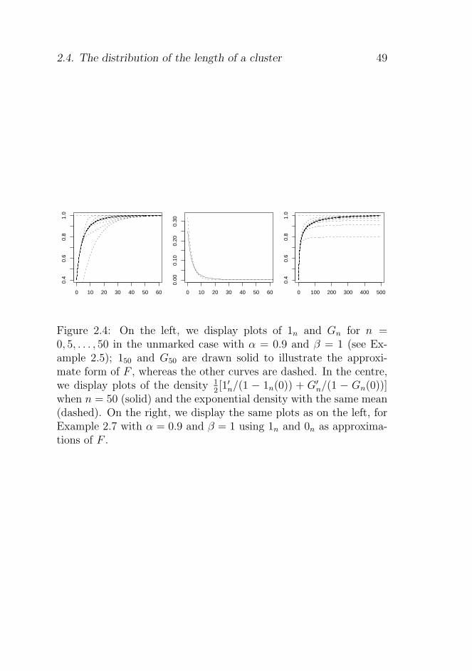
2.4. The distribution of the length of a cluster 49
0 10 20 30 40 50 60
0.4
0.6
0.8
1.0
0 10 20 30 40 50 60
0.00
0.10
0.20
0.30
0 100 200 300 400 5000.
40.
60.
81.
0
Figure 2.4: On the left, we display plots of 1n and Gn for n =0, 5, . . . , 50 in the unmarked case with α = 0.9 and β = 1 (see Ex-ample 2.5); 150 and G50 are drawn solid to illustrate the approxi-mate form of F , whereas the other curves are dashed. In the centre,we display plots of the density 1
2[1′n/(1 − 1n(0)) + G′
n/(1 − Gn(0))]when n = 50 (solid) and the exponential density with the same mean(dashed). On the right, we display the same plots as on the left, forExample 2.7 with α = 0.9 and β = 1 using 1n and 0n as approxima-tions of F .
50 Chapter 2. Perfect simulation of Hawkes processes
Example 2.6 (Birth-death process) For the case in Example 2.2,
L(θ) = E
∫ Z
0
eθs
EZds =
LZ(θ) − 1
θEZ
where LZ(θ) = EeθZ is the Laplace transform of Z. In the specialcase where Z is exponentially distributed with mean 1/β, L(θ) =LZ(θ) = β/(β − θ) is of the same form as in Example 2.5. Plots of1n, Gn, and
1
2
(
1′n1 − 1n(0)
+G′
n
1 −Gn(0)
)
for n = 0, 5, . . . , 50 and (α, β) = (0.9, 1) are similar to those in theleft-hand and centre panels of Figure 2.4 and are therefore omitted.2
Example 2.7 (Heavy-tailed distribution for L) For the case in Ex-ample 2.3, Proposition 2.3 does not apply, as L(θ) = ∞ for all θ > 0.The CDF in (2.25) is not known on closed form, since the convolu-tions are not tractable (in fact, this is the case when h specifies anyknown heavy-tailed distribution, including the Pareto, Weibull, log-normal or loggamma distribution). Nonetheless, it is still possible toget an idea of what F looks like: the right-hand panel of Figure 2.4shows 1n and 0n for n = 0, 5, . . . , 50 in the case (α, β) = (0.9, 1). Asin Examples 2.5 and 2.6, the convergence of 1n and Gn (where, now,G = 0) and the approximate form of F are clearly visible. How-ever, as indicated by the plots and verified in Møller and Rasmussen(2004), limt→0Gn(t) < 1 when G = 0, meaning that Gn is not a CDF.2
2.5 Simulation of I2
To complete the perfect simulation algorithm (Algorithm 2.2), weneed a useful way of simulating I2. Our procedure is based on a
2.5. Simulation of I2 51
dominating process and the use of coupled upper and lower pro-cesses, in the spirit of the dominated-coupling-from-the-past algo-rithm (Kendall and Møller, 2000).
Suppose that f ∈ C is in closed form, with f ≤ ϕ(f), and that(2.9) is satisfied when we replace F by f (situations in which theserequirements are fulfilled are considered in Sections 2.3, 2.4.2 and2.4.3). Particularly, if µ is constant and f is a CDF, (2.9) impliesthat f has a finite mean. Now, for n ∈ N0, let Un and Ln denotePoisson processes on (−∞, 0) with intensity functions
λun(t) = (1 − fn(−t))µ(t) and λl
n(t) = (1 − 1n(−t))µ(t),
respectively. By Theorem 2.1, λun is nonincreasing and λl
n is nonde-creasing in n, and they both converge to λ2 (geometrically fast withrespect to the supremum norm). Consequently, we can use indepen-dent thinning to obtain the following sandwiching/funneling property(cf. Kendall and Møller (2000)):
∅ = L0 ⊆ L1 ⊆ L2 ⊆ · · · ⊆ I2 ⊆ · · · ⊆ U2 ⊆ U1 ⊆ U0. (2.27)
The details are given by the following algorithm.
Algorithm 2.3 (Simulation of I2.)
1. Generate a realization {(t1, Z1), . . . , (tk, Zk)} of U0, where t1 <. . . < tk.
2. If U0 = ∅, then return I2 = ∅ and stop; otherwise generate inde-pendent uniform numbers W1, . . . ,Wk on [0, 1] (independentlyof U0), and set n = 1.
3. For j = 1, . . . , k, assign (tj, Zj) to Ln or Un if Wjλu0(tj) ≤ λl
n(tj)or, respectively, Wjλ
u0(tj) ≤ λu
n(tj).
4. If Un = Ln, then return I2 = Ln and stop; otherwise increase nby 1 and repeat steps (3)–(4).
52 Chapter 2. Perfect simulation of Hawkes processes
Proposition 2.4 Algorithm 2.3 works correctly and terminates al-most surely within finite time.
Proof. To see this, imagine that, regardless of whether U0 = ∅ in step(2) or Un = Ln in step (4), we continue to generate (U1, L1), (U2, L2),etc. Furthermore, add an extra step: for j = 1, . . . , k, assign (tj, Zj)to I2 if and only if
Wjλun(tj) ≤ λ2(tj).
Then clearly, because of the convergence properties of λun and λl
n (seethe discussion above), (2.27) is satisfied and, conditional on t1, . . . , tk,
P(Ln 6= Un for all n ∈ N0)
≤k∑
j=1
limn→∞
P(Wjλu0(tj) ≤ λu
n(tj), Wjλu0(tj) > λl
n(tj))
=k∑
j=1
P(λ2(tj) < Wjλu0(tj) ≤ λ2(tj)) = 0.
Thus, almost surely Algorithm 2.3 terminates within finite time andthe output equals I2. 2
Remark 2.5 We compute 1n and fn numerically, using a quadraturerule (see Remark 2.3). After step (1) in Algorithm 2.3, we let the lastquadrature point be given by −t1 (since we do not need to calculate1n(t) and fn(t) for t > −t1). Since we have to calculate 1n andfn recursively for all n = 0, 1, 2, . . . until Algorithm 2.3 terminates,there is no advantage in using a doubling scheme for n, as in thePropp-Wilson algorithm (Propp and Wilson, 1996). 2
Example 2.8 (Birth-death process.) We have checked our computercode for Algorithms 2.2 and 2.3 by comparing with results producedby another perfect simulation algorithm. Consider the case in Exam-ple 2.2 when µ(t) = µ is constant and Z is exponentially distributedwith mean 1/β. If N denotes the number of events alive at time 0,
2.6. Extensions and open problems 53
we have the following detailed balance condition for its equilibriumdensity πn:
πn(µ+ αβn) = πn+1β(n+ 1), n ∈ N0.
This density is well defined, since limn→∞ πn+1/πn = α < 1. Now,choose m ∈ N0 and ǫ ≥ 0 such that a = α + ǫ < 1 and πn+1/πn ≤ awhenever n ≥ m. If µ ≤ αβ, we can take ǫ = m = 0; otherwise, wecan use m ≥ (µ− αβ)/(βǫ) for some ǫ > 0. Define an unnormalizeddensity π′
n, n ∈ N0, by π′n = πn/π0 if n ≤ m, and π′
n = an−mπm/π0
otherwise. We can easily sample from π′n by inversion (see Ripley
(1987)), since we can calculate
∞∑
0
π′n =
m∑
0
πn
π0
+a
1 − a
πm
π0
.
Then, since π′n ≥ πn/π0, we can sample N from πn by rejection
sampling (see Ripley (1987)). Furthermore, conditional on N = n,we generate n independent marks Z ′
1, . . . , Z′n that are exponentially
distributed with mean 1/β (here, we exploit the memoryless propertyof the exponential distribution). Finally, we simulate the markedHawkes process with events in (0, t+], using the conditional intensity
λ′(t) = µ+ αβ
(
n∑
i=1
1[t < Z ′i] +
∑
0<ti<t
1[t < ti + Zi]
)
.
We have implemented this algorithm for comparison with our al-gorithm. Not surprisingly, it is a lot faster than our perfect simulationalgorithm (roughly 1200 times as fast in the case α = 0.9, β = µ = 1,and t+ = 10), since it exploits the fact that we know the stationarydistribution in this special case. 2
2.6 Extensions and open problems
Except for the heavy-tailed case, our perfect simulation algorithm isfeasible in the examples we have considered. However, simulation
54 Chapter 2. Perfect simulation of Hawkes processes
of the heavy-tailed cases is an unsolved problem. In these cases,we can only say something about the approximate form of F (seeExample 2.7).
For applications such as in seismology (Ogata, 1998), extensionsof our results and algorithms to the heavy-tailed cases are impor-tant. The epidemic type aftershock sequences (ETAS) model (Ogata(1988)) used for modeling times and magnitudes of earthquakes, isa heavy-tailed marked Hawkes process. Its spatio-temporal exten-sion, which also includes the locations of the earthquakes (see Ogata(1998)), furthermore involves the problem of predictable marks (thelocation of an aftershock depends on the location of the earthquakethat causes it). This problem is easily solved, though, since the timesand magnitudes are independent of the locations and can be simu-lated without worrying about these. This, of course, still leaves theunsolved problem of the heavy tails.
Extensions to nonlinear Hawkes processes (Bremaud and Mas-soulie, 1996; Daley and Vere-Jones, 2003) would also be interesting.However, things again become complicated, since a nonlinear Hawkesprocess is not even a Poisson cluster process.
Simulations of Hawkes processes with predictable marks can, insome cases, be obtained by using a thinning algorithm, if it is possibleto dominate the Hawkes process with predictable marks by a Hawkesprocess with unpredictable marks. We illustrate the procedure witha simple birth-death example.
Example 2.9 (Birth-death process) Consider two birth-death Haw-kes processes as defined in Example 2.2. Let Ψ1 have unpredictablemarks, with Z1
i ∼ Exp(β), and let Ψ2 have predictable marks, withZ2
i ∼ Exp(β + 1/Z2An), where Z2
An is the mark of the first order an-cestor of ti. Both models have γ(t, Z) = αβ1[t < Z], with the sameα and β, and they also have the same µ(t). The model Ψ2 has the in-tuitive appeal that long-living individuals have long-living offspring.Note that the intensity of Ψ1 dominates the intensity of Ψ2 if themarks are simulated such that Z1
i > Z2i .
2.6. Extensions and open problems 55
To simulate Ψ2, we first simulate Ψ1 using Algorithm 2.3, withthe modifications that we associate both marks Z1
i and Z2i to the
event ti, and we keep all events from the algorithm whether they fallin or before [0, t+). Each marked event (tj, Z
1j ) is then included in
Ψ2 with retention probability
µ(t) + αβ∑
ti<tj ,ti∈Ψ21[tj − ti < Z2
i ]
µ(t) + αβ∑
ti<tj1[tj − ti < Z1
i ]
and the final output is all marked events from Ψ2 falling in [0, t+). Itis easily proven that these retention probabilities result in the correctprocess Ψ2. 2
Another process that would be interesting to obtain by thinning isthe Hawkes process without immigrants considered in Bremaud andMassoulie (2001); this process has µ(t) = 0 for all t. However, forthis to be non-trivial (i.e. not almost surely empty), it is necessarythat ν = 1, which means that any dominating Hawkes process hasν ≥ 1 and, thus, cannot be simulated by Algorithm 2.3.
Many of our results and algorithms can be modified if we slightlyextend the definition in Section 2.1 of a marked Hawkes process, asfollows. For any event ti with associated mark Zi, let ni denote thenumber of (first generation) offspring generated by (ti, Zi), and sup-pose that ni, conditional on Zi, is not necessarily Poisson distributed,but ni is still conditionally independent of ti and the previous history.A particular simple case occurs when ni is either 1 or 0, and
p = E[P(ni = 1|Zi)]
is assumed to be strictly between 0 and 1 (here p plays a similar roleas ν introduced in Section 2.4). Then we redefine ϕ by
ϕ(f)(t) = 1 − p+ p
∫ t
0
f(t− s)h(s) ds
where, now,h(s) = E(p(Z)h(s, Z))/p.
56 Chapter 2. Perfect simulation of Hawkes processes
Since ϕ is now linear, the situation is much simpler. For example, Fis given by G in (2.25) (with ν replaced by p).
Another extension of practical relevance is to consider a non-Poisson immigrant process, e.g. a Markov or Cox process. The resultsin Section 2.4 do not depend on the choice of immigrant process, andthe straightforward simulation algorithm (Algorithm 2.1) applies pro-vided it is feasible to simulate the immigrants on [t−, t+). However,the perfect simulation algorithm relies much on the assumption thatthe immigrant process is Poisson.
Finally, we notice that it would be interesting to extend ourideas to spatial Hawkes processes (see Møller and Torrisi (2004a)and Møller and Torrisi (2004b)).
Acknowledgements
We are grateful to Søren Asmussen, Svend Berntsen, Horia Cornean,Martin Jacobsen, Arne Jensen, and Giovanni Luca Torrisi for help-ful discussions. The research of Jesper Møller was supported by theDanish Natural Science Research Council and the Network in Mathe-matical Physics and Stochastics (MaPhySto), funded by grants fromthe Danish National Research Foundation.
References
Apostol, T. M. (1974). Mathematical Analysis . Addison-Wesley,Reading.
Asmussen, S. (1987). Applied Probability and Queues . Wiley, Chich-ester.
Bremaud, P. and Massoulie, L. (1996). Stability of nonlinear Hawkesprocesses. Ann. Prob., 24, 1563–1588.
2.6. Extensions and open problems 57
Bremaud, P. and Massoulie, L. (2001). Hawkes branching point pro-cesses without ancestors. J. Appl. Prob., 38, 122–135.
Bremaud, P., Nappo, G., and Torrisi, G. (2002). Rate of convergenceto equilibrium of marked Hawkes processes. J. Appl. Prob., 39,123–136.
Brix, A. and Kendall, W. (2002). Simulation of cluster point processeswithout edge effects. Adv. Appl. Prob., 34, 267–280.
Chornoboy, E. S., Schramm, L. P., and Karr, A. F. (2002). Maximumlikelihood identification of neural point process systems. Adv. Appl.Prob., 34, 267–280.
Daley, D. J. and Vere-Jones, D. (2003). An Introduction to the Theoryof Point Processes, Volume I: Elementary Theory and Methods .Springer, New York, 2nd edition.
Dwass, M. (1969). The total progeny in a branching process and arelated random walk. J. Appl. Prob., 6, 682–686.
Hawkes, A. G. (1971a). Point spectra of some mutually exciting pointprocesses. J. Roy. Statist. Soc. Ser. B , 33, 438–443.
Hawkes, A. G. (1971b). Spectra of some self-exciting and mutuallyexciting point processes. Biometrika, 58(1), 83–90.
Hawkes, A. G. (1972). Spectra of some mutually exciting point pro-cesses with associated variables. In P. A. W. Lewis, editor, Stochas-tic Point Processes , pages 261–271. Wiley, New York,.
Hawkes, A. G. and Adamopoulos, L. (1973). Cluster models forearthquakes – regional comparisons. Bull. Int. Statist. Inst., 45,454–461.
Hawkes, A. G. and Oakes, D. (1974). A cluster representation of aself-exciting process. J. Appl. Prob., 11, 493–503.
58 Chapter 2. Perfect simulation of Hawkes processes
Jagers, P. (1975). Branching Processes with Biological Applications .John Wiley & Sons, London.
Kendall, W. S. and Møller, J. (2000). Perfect simulation using dom-inating processes on ordered spaces, with application to locallystable point processes. Adv. Appl. Prob., 32, 844–865.
Møller, J. (2003). Shot noise Cox processes. Adv. Appl. Prob., 35,614–640.
Møller, J. and Rasmussen, J. G. (2004). Approximate simula-tion of Hawkes processes. Research report R-2004-28, Depart-ment of Mathematical Sciences, Aalborg University. Available athttp://www.math.aau.dk/ jm.
Møller, J. and Torrisi, G. L. (2004a). Generalised shotnoise Cox processes. Research report R-2004-07, Depart-ment of Mathematical Sciences, Aalborg University. Available athttp://www.math.aau.dk/ jm.
Møller, J. and Torrisi, G. L. (2004b). Perfect and approximate sim-ulation of spatial Hawkes processes. In preparation.
Møller, J. and Waagepetersen, R. P. (2004). Statistical Inference andSimulation for Spatial Point Processes . Chapman & Hall, BocaRaton, Florida.
Ogata, Y. (1988). Statistical models for earthquake occurrences andresidual analysis for point processes. J. Amer. Statist. Assoc.,83(401), 9–27.
Ogata, Y. (1998). Space-time point-process models for earthquakeoccurrences. Ann. Inst. Statist. Math., 50(2), 379–402.
Propp, J. G. and Wilson, D. B. (1996). Exact sampling with coupledMarkov chains and applications to statistical mechanics. RandomStructures and Algorithms, 9, 223–252.

2.6. Extensions and open problems 59
Ripley, B. D. (1987). Stochastic Simulation. Wiley, New York.
Rudin, W. (1987). Real and Complex Analysis . McGraw-Hill, NewYork.
Vere-Jones, D. and Ozaki, T. (1982). Some examples of statisticalinference applied to earthquake data. Ann. Inst. Statist. Math.,34, 189–207.

60 Chapter 2. Perfect simulation of Hawkes processes
Chapter 3
Approximate simulation of
Hawkes processes
Jesper Møller & Jakob G. Rasmussen
Department of Mathematical Sciences, Aalborg University, FredrikBajers Vej 7G, DK-9220 Aalborg, Denmark.
Email addresses: [email protected] & [email protected]
Abstract
Hawkes processes are important in point process theory and its appli-cations, and simulation of such processes are often needed for variousstatistical purposes. This article concerns a simulation algorithm forunmarked and marked Hawkes processes, exploiting that the processcan be constructed as a Poisson cluster process. The algorithm suf-fers from edge effects but is much faster than the perfect simulationalgorithm introduced in our previous work Møller and Rasmussen(2004). We derive various useful measures for the error committedwhen using the algorithm, and we discuss various empirical resultsfor the algorithm compared with perfect simulations. Extensions of
61
62 Chapter 3. Approximate simulation of Hawkes processes
the algorithm and the results to more general types of marked pointprocesses are also discussed.
Keywords: Edge effects; Hawkes process; marked point process; Pois-son cluster process; simulation.
2000 Mathematical Subject Classification: Primary 60G55Secondary 68U20
3.1 Introduction
This paper concerns a useful simulation algorithm for unmarked andmarked Hawkes processes (Hawkes, 1971a,b, 1972; Hawkes and Oakes,1974; Daley and Vere-Jones, 2003). Such processes are important inpoint process theory and its applications, cf., for example, p. 183in Daley and Vere-Jones (2003). Particularly, marked Hawkes pro-cesses have applications in seismology (Hawkes and Adamopoulos,1973; Vere-Jones and Ozaki, 1982; Ogata, 1988, 1998) and neuro-physiology (Chornoboy et al., 2002). The algorithm in this papersuffers from edge effects but is of more practical importance than theperfect simulation algorithm introduced in Møller and Rasmussen(2004).
There are many ways to define a marked Hawkes process, but forour purpose it is most convenient to define it as a marked Poissoncluster process X = {(ti, Zi)} with events (or times) ti ∈ R andmarks Zi defined on an arbitrary (mark) space M equipped with aprobability distribution Q. The cluster centres of X correspond tocertain events called immigrants and the rest of the events are calledoffspring.
Definition 3.1 (Hawkes process with unpredictable marks)
(a) The immigrants follow a Poisson process with a locally inte-grable intensity function µ(t), t ∈ R.
(b) The marks associated to the immigrants are i.i.d. with distri-bution Q and independent of the immigrants.
3.1. Introduction 63
(c) Each immigrant ti generates a cluster Ci, which consists ofmarked events of generations of order n = 0, 1, . . . with thefollowing branching structure: First we have (ti, Zi), which issaid to be of generation zero. Recursively, given the 0, . . . , ngenerations in Ci, each (tj, Zj) ∈ Ci of generation n generates aPoisson process Φj of offspring of generation n+1 with intensityfunction γj(t) = γ(t − tj, Zj), t > tj. Here γ is a non-negativemeasurable function defined on (0,∞). We refer to Φj as an off-spring process, and to γj and γ as fertility rates. Furthermore,the associated mark Zk to any offspring tk ∈ Φj has distribu-tion Q and Zk is independent of tk and all (tl, Zl) with tl < tk.As in Daley and Vere-Jones (2003) we refer to this as the caseof unpredictable marks.
(d) The clusters given the immigrants are independent.
(e) Finally, X consists of the union of all clusters.
Simulation procedures for Hawkes processes are needed for variousreasons: Analytical results are rather limited due to the complexstochastic structure; statistical inference, especially model checkingand prediction require simulations; displaying simulated realisationsof specific model constructions provide a better understanding of themodel. The general approach for simulating a (marked or unmarked)point process is to use a thinning algorithm such as Shedler-Lewisthinning algorithm or Ogata’s modified thinning algorithm, see e.g.Daley and Vere-Jones (2003). However, Definition 3.1 immediatelyleads to the following simpler and more efficient simulation algorithm,where t− ∈ [−∞, 0] and t+ ∈ (0,∞] are user-specified parameters,and the output is all marked points (ti, Zi) with ti ∈ [0, t+).
Algorithm 3.1 The following steps (i)-(ii) generate a simulation ofthose marked events (ti, Zi) ∈ X with 0 ≤ ti < t+.
(i) Simulate the immigrants on [t−, t+).
64 Chapter 3. Approximate simulation of Hawkes processes
(ii) For each such immigrant ti, simulate Zi and those (tj, Zj) ∈ Ci
with ti < tj < t+.
Usually in applications steps (i) and (ii) are easy because (a)–(c)in Definition 3.1 are straightforward. As discussed in Section 3.4.4,Algorithm 3.1 and many of our results apply or easily extend to thecase where the immigrant process is non-Poisson.
Ideally we should take t− = −∞, but in practice we need todetermine t− such that
∫ 0
t−
µ(t) dt < ∞. When∫ t
−
−∞µ(t) dt > 0,
Algorithm 3.1 suffers from edge effects, since clusters generated byimmigrants before time t− may contain offspring in [0, t+). The ob-jective in this paper is to quantify these edge effects and to compareAlgorithm 3.1 with the perfect simulation algorithm in Møller andRasmussen (2004).
The paper is organised as follows. Section 3.2 contains some pre-liminaries. Section 3.3 contains some convergence results needed inthis paper. In Section 3.4 various quantitative results for edge ef-fects are introduced, and among other things we relate our resultsto those in Bremaud et al. (2002) (which concerns approximate sim-ulation of a stationary marked Hawkes process with unpredictablemarks). Section 3.5 presents various examples of applications andempirical results for Algorithm 3.1, Ogata’s modified thinning algo-rithm and the perfect simulation algorithm in Møller and Rasmussen(2004).
3.2 Preliminaries
Let F denote the c.d.f. (cumulative distribution function) for L, thelength of a cluster, i.e. the time between the immigrant and the lastevent of the cluster. Consider the mean number of events in anyoffspring process Φi, ν ≡ Eν, where
ν =
∫ ∞
0
γ(t, Z) dt
3.3. Approximations of F 65
is the total fertility rate of an offspring process and Z denotes ageneric mark with distribution Q. We assume that
0 < ν < 1, (3.1)
which among other places is needed in Proposition 3.1. This as-sumption is discussed in detail in Bremaud and Massoulie (2001)and Møller and Rasmussen (2004). Finally, let
h(t) = Eγ(t, Z)/ν, t > 0, (3.2)
which can be interpreted as the normalised intensity function for thefirst generation of offspring in a cluster started at time 0.
3.3 Approximations of F
It turns out that F is unknown even for very simple cases of Hawkesprocesses, cf. Møller and Rasmussen (2004).
We first recall some convergence results from Møller and Ras-mussen (2004) and next establish a new useful result (Proposition 3.1)which provide useful approximations of F .
For n ∈ N0, let 1n denote the c.d.f. for the length of a clusterwhen all events of generation n + 1, n + 2, . . . are removed. Clearly,1n is decreasing in n, 1n → F pointwise as n→ ∞, and
10(t) = 1, t ≥ 0. (3.3)
Let C denote the class of Borel functions f : [0,∞) 7→ [0, 1]. Forf ∈ C, define ϕ(f) ∈ C by
ϕ(f)(t) = E
[
exp
(
−ν +
∫ t
0
f(t− s)γ(s, Z) ds
)]
, t ≥ 0. (3.4)
Then, as verified in Møller and Rasmussen (2004) the assumption ofunpredictable marks implies that
1n = ϕ(1n−1), n ∈ N, (3.5)
66 Chapter 3. Approximate simulation of Hawkes processes
and
F = ϕ(F ). (3.6)
The recursion (3.5) provides a useful numerical approximation toF . As the integral in (3.4) with f = 1n−1 quickly becomes diffi-cult to evaluate analytically as n increases, we compute the integralnumerically, using a quadrature rule.
Convergence with respect to the supremum norm of 1n and certainother functions towards F is established in Møller and Rasmussen(2004). In this paper establishing convergence with respect to theL1-norm becomes relevant. We let C1 denote the class of functionsf ∈ C with ‖F − f‖1 <∞, where ‖g‖1 =
∫∞
0|g(t)| dt is the L1-norm.
Proposition 3.1 With respect to the L1-norm, ϕ is a contractionon C1, that is, for all f, g ∈ C1 and n ∈ N, we have that fn, gn ∈ C1
and
‖ϕ(f) − ϕ(g)‖1 ≤ ν‖f − g‖1. (3.7)
Furthermore, F is the unique fixpoint,
‖F − fn‖1 → 0 as n→ ∞, (3.8)
and if either f ≤ ϕ(f) or f ≥ ϕ(f), then fn increases respectivelydecreases towards F with a geometric rate:
‖F − fn‖1 ≤νn
1 − ν‖ϕ(f) − f‖1. (3.9)
Proof. Let f, g ∈ C1. Recall that by the mean value theorem (e.g.Theorem 5.11 in Apostol (1974)), for any real numbers x and y,ex − ey = (x− y)ez(x,y), where z(x, y) is a real number between x andy. Thus by (3.4),
‖ϕ(f) − ϕ(g)‖1
=
∫ ∞
0
∣
∣
∣
∣
E
[
e−νec(t,f,g)
∫ t
0
(f(t− s) − g(t− s))γ(s, Z)ds
]∣
∣
∣
∣
dt (3.10)

3.3. Approximations of F 67
where c(t, f, g) is a random variable between∫ t
0f(t−s)γ(s, Z) ds and
∫ t
0g(t− s)γ(s, Z) ds. Since f, g ≤ 1, we obtain ec(t,f,g) ≤ eν , cf. (3.1).
Consequently,
‖ϕ(f) − ϕ(g)‖1 ≤
∫ ∞
0
∣
∣
∣
∣
E
[∫ t
0
(f(t− s) − g(t− s))γ(s, Z) ds
]∣
∣
∣
∣
dt
(3.11)
≤ E
[∫ ∞
0
∫ ∞
0
|f(u) − g(u)| du γ(s, Z) ds
]
= ν ‖f − g‖1
(3.12)
where in the latter inequality we have used first the triangle in-equality, next Fubini’s theorem, and finally a simple transformation.Thereby (3.7) is verified. The remaining part is verified along similarlines as in the proof of Theorem 1 in Møller and Rasmussen (2004)(with the minor observations that F is the unique fixpoint becauseof (3.8), and that we use monotone convergence when establishing(3.9)). 2
Remark 3.1 The following observation motivates why we restrictattention to the class C1 in Proposition 3.1, at least when consideringfunctions f ∈ C such that f ≤ F : For such functions f convergencefails as
‖F − f‖1 = ∞ ⇒ ‖F − fn‖1 = ∞, n ∈ N. (3.13)
To verify this, consider two non-negative Borel functions f ≤ g de-fined on [0,∞). Then as in (3.10)–(3.12), but now observing thatc(t, f, g) is between 0 and ν,
‖ϕ(f) − ϕ(g)‖1 ≥ E
[∫ ∞
0
∫ ∞
0
(g(u) − f(u))e−νγ(s, Z) ds du
]
= ‖f − g‖1E[νe−ν ].
By (3.1), E[νe−ν ] > 0, and so letting g = F , we obtain (3.13) whenn = 1, whereby (3.13) follows by induction.

68 Chapter 3. Approximate simulation of Hawkes processes
As noted the sequence fn = 1n decreases towards F pointwise. Inorder to obtain L1-convergence by Proposition 3.1 we need 10 ∈ C1,that is, EL = ‖1−F‖1 is finite. A sufficient and necessary conditionfor this is given in Lemma 1 in Møller and Rasmussen (2004).
To construct a sequence fn which increases towards F in the L1-norm, it suffices to find f ∈ C1 such that f ≤ ϕ(f). Methods for find-ing a c.d.f. G with G ≤ ϕ(G) are discussed in Møller and Rasmussen(2004) (see in particular Proposition 3 in Møller and Rasmussen(2004)), in which case G ≤ F (see Theorem 1 in Møller and Ras-mussen (2004)). Note that ifG ≤ F is a c.d.f. and ‖1−F‖1 <∞, thenG needs to have a finite mean, since ‖1−G‖1 = ‖F −G‖1 +‖1−F‖1.2
3.4 Edge effects
Let N(t−, t+) denote the number of missing events when using Algo-rithm 3.1. In this section we consider the mean number of missingoffspring, E(t−, t+) ≡ EN(t−, t+), and the probability of having anymissing offspring, P(t−, t+) ≡ P(N(t−, t+) > 0). Furthermore, werelate these to the total variation distance between simulations andthe target distribution.
3.4.1 The mean number of missing offspring
Consider a cluster C0 = {(si, Zi)} started at time t0 = 0. This hasconditional intensity function
λ0(t) = γ(t, Z0) +∑
0<si<t
γ(t− si, Zi), t ≥ 0, (3.14)
and unpredictable marks with distribution Q. For t > 0, let λ(t) =Eλ0(t) be the intensity function of the offspring in C0, and γ(t) =Eγ(t, Z) = νh(t) be the intensity function of the first generation ofoffspring in C0. The following proposition expresses E(t−, t+) andλ(t) in terms of µ and γ.
3.4. Edge effects 69
Proposition 3.2 We have that
λ(t) =∞∑
n=1
γ∗n(t) =∞∑
n=1
νnh∗n(t), t ≥ 0, (3.15)
where ∗n denotes convolution n times, and
E(t−, t+) =
∫ t−
−∞
(∫ t+−t
−t
λ(s) ds
)
µ(t) dt. (3.16)
Proof. We claim that ρn = γ∗n is the intensity function of Gn, then-th generation of offspring in the cluster C0: This is clearly true forn = 1, and so by induction
ρn+1(t) = E∑
si∈Gn
γ(t− si, Zi) = E∑
si∈Gn
E[γ(t− si, Zi)|si]
= E∑
si∈Gn
γ(t− si) =
∫ t
0
ρn(s)γ(t− s) ds = γ∗(n+1)
where we have used Campbell’s theorem in the second last equalityand the induction hypothesis in the last equality. Thereby (3.15)follows. Finally, if I denotes the Poisson process of immigrants,
E(t−, t+) = E∑
ti∈I
∑
s∈Ci
1[ti < t−, 0 ≤ s < t+]
= E∑
ti∈I: ti<t−
E
[
∑
s∈Ci
1[0 ≤ s < t+]
∣
∣
∣
∣
ti
]
= E∑
ti∈I: ti<t−
∫ t+−ti
−ti
λ(u) du
which reduces to (3.16) by Campbell’s theorem. 2
The convolution γ∗n is only computable for a few kinds of models(see Section 3.5).
70 Chapter 3. Approximate simulation of Hawkes processes
Remark 3.2 It follows immediately that
ρ = µ+ µ ∗ λ (3.17)
is the intensity function of all events. When quantifying edge effectsit is natural to consider E(t−, t+)/E(t+), where
E(t+) =
∫ t+
0
ρ(t) dt
is the expected number of events on [0, t+]. 2
3.4.2 The probability of having any missing off-
spring
Obviously, P(t−, t+) is an increasing function of t+ ∈ (0,∞]. Proposi-tion 3.3 gives an expression and upper and lower bounds for P(t−,∞).
Proposition 3.3 We have that
P(t−,∞) = 1 − exp
(
−
∫ t−
−∞
(1 − F (−t))µ(t) dt
)
. (3.18)
Further, for any f ∈ C1 such that f ≤ ϕ(f), we have an upper bound,
P(t−,∞) ≤ 1 − exp
(
−
∫ t−
−∞
(1 − fn(−t))µ(t) dt
)
, (3.19)
which is a decreasing function of n, and a lower bound
P(t−,∞) ≥ 1 − exp
(
−
∫ t−
−∞
(1 − 1n(−t))µ(t) dt
)
, (3.20)
which is a increasing function of n.

3.4. Edge effects 71
Proof. Let It−
be the point process of immigrants ti < t− with{(tj, Zj) ∈ Ci : tj ≥ 0} 6= ∅. Then It
−
is a Poisson process withintensity function λt
−
(t) = (1 − F (−t))µ(t) on (−∞, t−), since wecan view It
−
as an independent thinning of the immigrant processon (−∞, t−), with retention probabilities p(t) = 1 − F (−t), t <t−. Hence, since P(t−,∞) equals the probability that It
−
6= ∅, weobtain (3.18). Thereby (3.19) and (3.20) follows from (3.18) andProposition 3.1. 2
Remark 3.3 Proposition 3.1 ensures that the upper bound in (3.19)and the lower bound in (3.20) converge monotoneously to P(t−,∞)provided e.g. that µ is bounded and EL <∞, cf. Remark 3.1. 2
3.4.3 The total variation distance between simu-
lations and the target distribution
Recently, Bremaud et al. (2002) derived related results to Proposi-tions 3.2 and 3.3 when µ(t) is constant and t+ = ∞. Proposition 3.4below generalises certain inequalities in Bremaud et al. (2002) (page133, line 3 from below, and equation (3.13)) to the situation in thepresent paper where µ(t) is not necessarily constant and t+ may befinite. Moreover, our proof is much simpler.
We let X be another marked Hawkes process obtained from X byremoving all clusters Ci with immigrants ti < t−. Furthermore, we letY and Y denote the restriction of X and X to the marked events on[0, t+), and denote their distributions by π(t−, t+) and π(t−, t+). Thusthe output of Algorithm 3.1 follows π(t−, t+), which approximates thetarget distribution π(t−, t+).
Proposition 3.4 Let ‖·‖TV denote the total variation distance, then
‖π(t−, t+) − π(t−, t+)‖TV ≤ P(t−, t+) ≤ E(t−, t+). (3.21)
Proof. By the construction of Y , we have that Y ⊆ Y . The firstinequality then follows immediately from the coupling inequality (see
72 Chapter 3. Approximate simulation of Hawkes processes
e.g. Lindvall (1992)), while the second inequality is trivially satisfied.2
Remark 3.4 In contrast to the first upper bound in (3.21) the sec-ond upper bound does not depend on knowing F or any approxima-tion of F , cf. Propositions 3.2 and 3.3. 2
3.4.4 Extensions and open problems
It would be of practical importance to extend our results to the caseof predictable marks. Proposition 3.4 is still true if the conditionalintensity function for X is larger than or equal to the conditionalintensity function for X; this follows by a thinning argument, cf.Daley and Vere-Jones (2003). However, this observation seems of lit-tle use, since the assumption of unpredictable marks is essential inthe proofs of (3.15) in Proposition 3.2 and (3.19)–(3.20) in Proposi-tion 3.3. Moreover, though (3.18) in Proposition 3.3 remains true, itis expected to be of limited use, since F is expected to be of a morecomplicated form in the case of predictable marks.
The following observations may also be of practical relevance.
Algorithm 3.1 applies for a non-Poisson immigrant process, e.g. aMarkov or Cox process provided it is feasible to simulate the immi-grants on [t−, t+). Furthermore, Proposition 3.2 remains true for anyimmigrant process with intensity function µ. Finally, Proposition 3.3partly relies on the immigrants being a Poisson process: for instance,if now µ is a random intensity function and the immigrant process isa Cox process driven by µ, then (3.18)–(3.20) should be modified bytaking the mean of the expressions on the right hand sides.
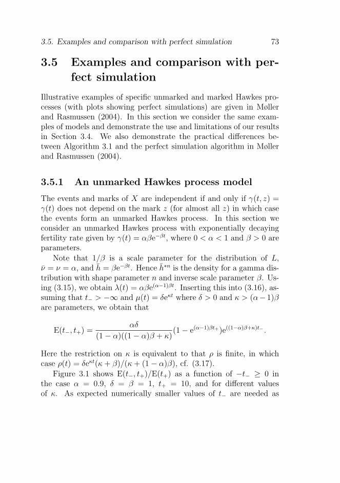
3.5. Examples and comparison with perfect simulation 73
3.5 Examples and comparison with per-
fect simulation
Illustrative examples of specific unmarked and marked Hawkes pro-cesses (with plots showing perfect simulations) are given in Møllerand Rasmussen (2004). In this section we consider the same exam-ples of models and demonstrate the use and limitations of our resultsin Section 3.4. We also demonstrate the practical differences be-tween Algorithm 3.1 and the perfect simulation algorithm in Møllerand Rasmussen (2004).
3.5.1 An unmarked Hawkes process model
The events and marks of X are independent if and only if γ(t, z) =γ(t) does not depend on the mark z (for almost all z) in which casethe events form an unmarked Hawkes process. In this section weconsider an unmarked Hawkes process with exponentially decayingfertility rate given by γ(t) = αβe−βt, where 0 < α < 1 and β > 0 areparameters.
Note that 1/β is a scale parameter for the distribution of L,ν = ν = α, and h = βe−βt. Hence h∗n is the density for a gamma dis-tribution with shape parameter n and inverse scale parameter β. Us-ing (3.15), we obtain λ(t) = αβe(α−1)βt. Inserting this into (3.16), as-suming that t− > −∞ and µ(t) = δeκt where δ > 0 and κ > (α−1)βare parameters, we obtain that
E(t−, t+) =αδ
(1 − α)((1 − α)β + κ)(1 − e(α−1)βt+)e((1−α)β+κ)t
− .
Here the restriction on κ is equivalent to that ρ is finite, in whichcase ρ(t) = δeκt(κ+ β)/(κ+ (1 − α)β), cf. (3.17).
Figure 3.1 shows E(t−, t+)/E(t+) as a function of −t− ≥ 0 inthe case α = 0.9, δ = β = 1, t+ = 10, and for different valuesof κ. As expected numerically smaller values of t− are needed as
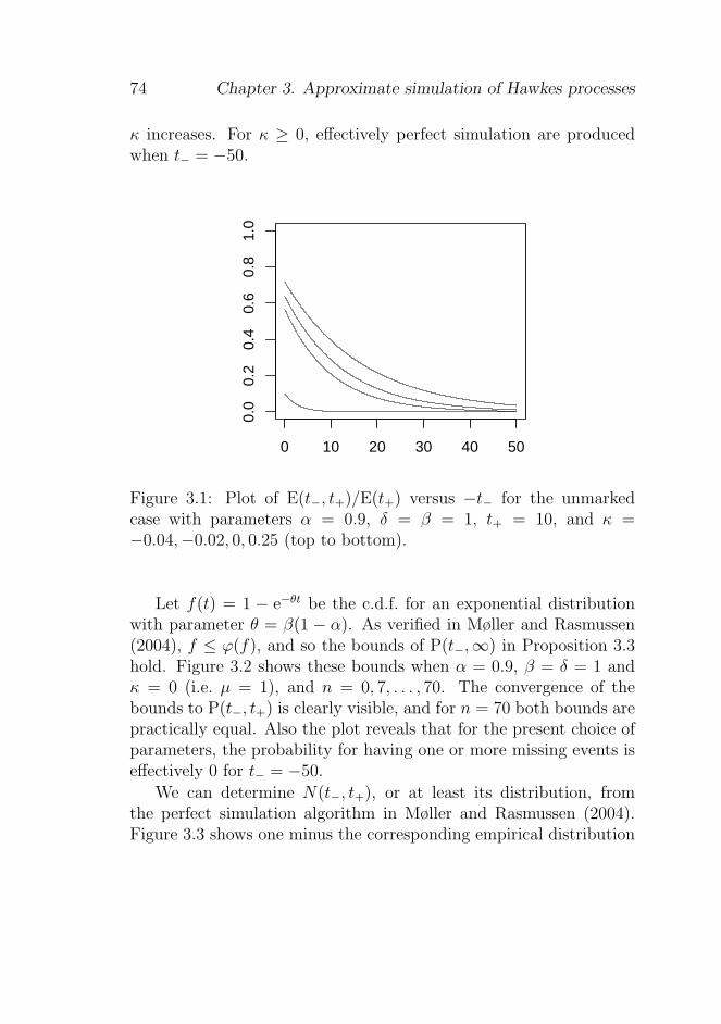
74 Chapter 3. Approximate simulation of Hawkes processes
κ increases. For κ ≥ 0, effectively perfect simulation are producedwhen t− = −50.
0 10 20 30 40 50
0.0
0.2
0.4
0.6
0.8
1.0
Figure 3.1: Plot of E(t−, t+)/E(t+) versus −t− for the unmarkedcase with parameters α = 0.9, δ = β = 1, t+ = 10, and κ =−0.04,−0.02, 0, 0.25 (top to bottom).
Let f(t) = 1 − e−θt be the c.d.f. for an exponential distributionwith parameter θ = β(1 − α). As verified in Møller and Rasmussen(2004), f ≤ ϕ(f), and so the bounds of P(t−,∞) in Proposition 3.3hold. Figure 3.2 shows these bounds when α = 0.9, β = δ = 1 andκ = 0 (i.e. µ = 1), and n = 0, 7, . . . , 70. The convergence of thebounds to P(t−, t+) is clearly visible, and for n = 70 both bounds arepractically equal. Also the plot reveals that for the present choice ofparameters, the probability for having one or more missing events iseffectively 0 for t− = −50.
We can determine N(t−, t+), or at least its distribution, fromthe perfect simulation algorithm in Møller and Rasmussen (2004).Figure 3.3 shows one minus the corresponding empirical distribution

3.5. Examples and comparison with perfect simulation 75
0 10 20 30 40 50
0.0
0.2
0.4
0.6
0.8
1.0
Figure 3.2: Upper and lower bounds (3.19) and (3.20) of P (t−, t+)versus −t− in the unmarked case with α = 0.9, µ = β = 1, t+ = ∞,and n = 0, 7, . . . , 70. The bounds using n = 70 are shown in blackto illustrate the approximate form of P(t−, t+), whereas the rest areshown in gray.
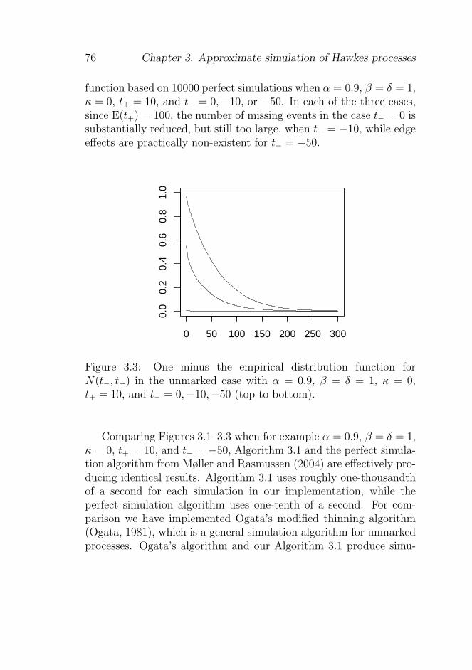
76 Chapter 3. Approximate simulation of Hawkes processes
function based on 10000 perfect simulations when α = 0.9, β = δ = 1,κ = 0, t+ = 10, and t− = 0,−10, or −50. In each of the three cases,since E(t+) = 100, the number of missing events in the case t− = 0 issubstantially reduced, but still too large, when t− = −10, while edgeeffects are practically non-existent for t− = −50.
0 50 100 150 200 250 300
0.0
0.2
0.4
0.6
0.8
1.0
Figure 3.3: One minus the empirical distribution function forN(t−, t+) in the unmarked case with α = 0.9, β = δ = 1, κ = 0,t+ = 10, and t− = 0,−10,−50 (top to bottom).
Comparing Figures 3.1–3.3 when for example α = 0.9, β = δ = 1,κ = 0, t+ = 10, and t− = −50, Algorithm 3.1 and the perfect simula-tion algorithm from Møller and Rasmussen (2004) are effectively pro-ducing identical results. Algorithm 3.1 uses roughly one-thousandthof a second for each simulation in our implementation, while theperfect simulation algorithm uses one-tenth of a second. For com-parison we have implemented Ogata’s modified thinning algorithm(Ogata, 1981), which is a general simulation algorithm for unmarkedprocesses. Ogata’s algorithm and our Algorithm 3.1 produce simu-
3.5. Examples and comparison with perfect simulation 77
lations with the same distribution; however, Ogata’s algorithm usesapproximately one-twentieth of a second to make an approximatesimulation.
3.5.2 A marked Hawkes process model with birth
and death transitions
Consider a marked Hawkes process with
γ(t, z) = α1[t ≤ z]/EZ,
where 0 < α < 1 is a parameter, Z is a positive random variablewith distribution Q, and 1[·] denotes the indicator function. ThenX can be viewed as a birth and death process, with birth at time tiand survival time Zi of the i’th individual (more general birth anddeath processes (even non-Markovian) are considered in Bremaudand Massoulie (2002) and Torrisi (2002)).
The special case where µ(t) = µ is constant and Z is exponentiallydistributed with mean 1/β is considered at page 136 in Bremaud et al.(2002). Since h(t) = βe−βt is the same function as in Section 3.5.1,E(t−, t+) is also the same as in Section 3.5.1. Further, a plot ofP (t−, t+) (omitted here) is similar to Figure 3.2 (when using thesame parameters). Also a plot of the empirical distribution functionof N(t−, t+) (omitted here) is similar to Figure 3.3.
When for example α = 0.9, β = µ = 1, t+ = 10, and t− = −50,Algorithm 3.1 uses roughly one-five hundredth of a second for eachsimulation, and the perfect simulation algorithm uses just under threeseconds. As in the unmarked case both algorithms are feasible, butthe difference is much more clear in the present case.
3.5.3 A heavy-tailed distribution for L
We conclude by observing that heavy-tailed cases of the distributionof L are problematic. For instance, suppose that
γ(t, z) = αze−tz, (3.22)

78 Chapter 3. Approximate simulation of Hawkes processes
where α ∈ (0, 1) is a parameter, and let Q be the exponential distri-bution with mean 1/β. As argued in Møller and Rasmussen (2004),h(t) = β/(t + β)2 is a Pareto density and L has a heavy-tailed dis-tribution with infinite moments and infinite Laplace transform. AsEL = ∞, Proposition 3.1 and hence Proposition 3.3 seem of ratherlimited use, cf. Remark 3.1. Proposition 3.2 in Bremaud et al. (2002)establish and upper bound for P (t−,∞) for such heavy-tailed casesunder certain mild conditions, however, in the case of 3.22 their re-sult does not apply. Proposition 3.2 is also not applicable, since λ isnot known on closed form, cf. Example 7 in Møller and Rasmussen(2004). It is a challenging open problem to handle such heavy-tailedcases.
Acknowledgements
The research of Jesper Møller was supported by the Danish NaturalScience Research Council and the Network in Mathematical Physicsand Stochastics (MaPhySto), funded by grants from the Danish Na-tional Research Foundation.
References
Apostol, T. M. (1974). Mathematical Analysis . Addison-Wesley,Reading.
Bremaud, P. and Massoulie, L. (2001). Hawkes branching point pro-cesses without ancestors. J. Appl. Prob., 38, 122–135.
Bremaud, P. and Massoulie, L. (2002). Power spectra of general shotnoises and Hawkes point processes with a random excitation. Adv.Appl. Prob., 34, 205–222.
Bremaud, P., Nappo, G., and Torrisi, G. (2002). Rate of convergence
3.5. Examples and comparison with perfect simulation 79
to equilibrium of marked Hawkes processes. J. Appl. Prob., 39,123–136.
Chornoboy, E. S., Schramm, L. P., and Karr, A. F. (2002). Maximumlikelihood identification of neural point process systems. Adv. Appl.Prob., 34, 267–280.
Daley, D. J. and Vere-Jones, D. (2003). An Introduction to the Theoryof Point Processes, Volume I: Elementary Theory and Methods .Springer, New York, 2nd edition.
Hawkes, A. G. (1971a). Point spectra of some mutually exciting pointprocesses. J. Roy. Statist. Soc. Ser. B , 33, 438–443.
Hawkes, A. G. (1971b). Spectra of some self-exciting and mutuallyexciting point processes. Biometrika, 58(1), 83–90.
Hawkes, A. G. (1972). Spectra of some mutually exciting point pro-cesses with associated variables. In P. A. W. Lewis, editor, Stochas-tic Point Processes , pages 261–271. Wiley, New York,.
Hawkes, A. G. and Adamopoulos, L. (1973). Cluster models forearthquakes – regional comparisons. Bull. Int. Statist. Inst., 45,454–461.
Hawkes, A. G. and Oakes, D. (1974). A cluster representation of aself-exciting process. J. Appl. Prob., 11, 493–503.
Lindvall, T. (1992). Lectures on the Coupling Method . Wiley, NewYork.
Møller, J. and Rasmussen, J. G. (2004). Perfect simulationof Hawkes processes. Research report R-2004-18, Depart-ment of Mathematical Sciences, Aalborg University. Available athttp://www.math.aau.dk.
Ogata, Y. (1981). On Lewis’ simulation method for point processes.IEEE Transactions on Information Theory , IT-27(1), 23–31.
80 Chapter 3. Approximate simulation of Hawkes processes
Ogata, Y. (1988). Statistical models for earthquake occurrences andresidual analysis for point processes. J. Amer. Statist. Assoc.,83(401), 9–27.
Ogata, Y. (1998). Space-time point-process models for earthquakeoccurrences. Ann. Inst. Statist. Math., 50(2), 379–402.
Torrisi, G. L. (2002). A class of interacting marked point processes:rate of convergence to equilibrium. J. Appl. Prob., 39, 137–160.
Vere-Jones, D. and Ozaki, T. (1982). Some examples of statisticalinference applied to earthquake data. Ann. Inst. Statist. Math.,34, 189–207.
Chapter 4
Spatial-temporal modeling
of forest gaps generated by
colonization from below-
and above-ground bark
beetle species
Jun Zhu
Department of Statistics, University of Wisconsin-Madison.
Email addresses: [email protected]
Jesper Møller & Jakob G. Rasmussen
Department of Mathematical Sciences, Aalborg University.
Email addresses: [email protected] & [email protected]
Brian H. Aukema & Kenneth F. Raffa
Department of Entomology, University of Wisconsin-Madison.
Email addresses: [email protected]
81

82 Chapter 4. Spatial-temporal modeling of forest gaps
Abstract
Studies of forest declines are important, because they both reducetimber production and affect successional trajectories of landscapesand ecosystems. Of particular interest is the decline of red pineswhich is characterized by expanding areas of dead and chlorotic treesin plantations throughout the Great Lakes Region. Here we examinethe impact of two bark beetle groups, namely red turpentine beetlesand pine engraver bark beetles, on tree mortality and the subsequentgap formation over time in a plantation in Wisconsin. We constructspatial-temporal statistical models that quantify the relations amongred turpentine beetle colonization, pine engraver bark beetle coloniza-tion, and mortality of red pine trees, while accounting for correlationacross space and over time. For statistical inference, we adopt aBayesian hierarchical model and devise Markov chain Monte Carloalgorithms for obtaining the posterior distributions of model param-eters as well as posterior predictive distributions. Our data analysisresults suggest that red turpentine beetle colonization is associatedwith higher likelihood of pine engraver bark beetle colonization andpine engraver bark beetle colonization is associated with higher likeli-hood of red pine tree mortality, whereas there is no direct associationbetween red turpentine beetle colonization and red pine tree mortal-ity. There is strong evidence that red turpentine beetle colonizationdoes not kill a red pine tree directly, but rather predisposes the treeto subsequent colonization by pine engraver bark beetles. The evi-dence is also strong that pine engraver bark beetles are the ultimatemortality agents of red pine trees.
Keywords: Autologistic model, Bayesian inference, forest entomol-ogy, Markov chain Monte Carlo, perfect simulation, spatial-temporalprocesses.
4.1. Introduction 83
4.1 Introduction
Studies of forest declines are of great interest to the timber indus-try, natural resource managers, and ecologists alike, because thesedeclines both reduce timber production and affect successional tra-jectories of landscapes and ecosystems. Decline syndromes occur inforests throughout the world, and occur at a variety of scales (Auclair,2005). Declines due to soil acidification and atmospheric pollutionmay affect large areas (Battles and Fahey, 2000; Drohan et al., 2002;Purdon et al., 2004) while declines due to insect and/or disease com-plexes may exhibit smaller mosaics of mortality such as gap forma-tion, which is our focus here (Klepzig et al., 1991; Erbilgin and Raffa,2003). In some systems, areas of large-scale mortality to insects andpathogens may originate from such small-scale mosaics. Character-izing spatial patterns and gaining inference about the processes thatmay create such patterns may assist in policy and management deci-sions when dealing with declines. Indeed, linking pattern and processis a key goal in ecology.
In particular we examine tree mortality and the subsequent gapformation over time in red pine forests. Decline of red pines is charac-terized by expanding areas, termed “pockets” of dead, slow growing,and chlorotic trees in plantations throughout the Great Lakes Region(Klepzig et al., 1991). Abiotic factors such as soil characteristics anddrought stress can predispose trees to biotic mortality agents such asinsects and root pathogens (Klepzig et al., 1991; Erbilgin and Raffa,2002). Here we focus on the impact of two bark beetle groups, called“turpentine beetles” and “Ips spp.” (for details of the species, seeSection 4.2), on the decline of red pines in a plantation in Wisconsin.
Past studies on red pine decline have yielded valuable insights onindividual components of this system by examining multiple levels ofscale, from detailed studies on individual trees (Klepzig et al., 1995;Raffa and Smalley, 1995; Klepzig et al., 1996) to regional studiescomparing multiple sites (Klepzig et al., 1991; Erbilgin and Raffa,2002, 2003). Despite these advances, elucidation of exact mechanisms
84 Chapter 4. Spatial-temporal modeling of forest gaps
of pocket development and expansion remain elusive since a single sitehas never been observed over more than three years. In the presentstudy, we examine a seven-year data set of annual surveys of all treesin a plantation. Each year, each of the 2,715 trees was examinedfor presence/absence of Ips spp., tree condition (alive/dead), andthe number of pitch tubes, each of which signifies colonization by aturpentine beetle. We attempt to answer several important ecologicalquestions. Of most interest is how the mortality rate of a tree isassociated with the turpentine beetle and Ips spp. colonization. Forexample, how different are the mortality rates between a tree thathas been colonized by both groups and a tree that has been colonizedby just one group of bark beetles? Related to these questions arethe degree of association between turpentine beetle and Ips spp. Forexample, what is the likelihood of a tree that has been colonizedby turpentine beetles will be colonized by Ips spp. subsequently?Moreover it is also of interest to quantify the spatial and temporalrelations among turpentine beetle colonization, Ips spp. colonization,and tree mortality.
The study of red pine declines poses statistical challenges, in thatprocesses giving rise to patterns of mortality may act at different lev-els of temporal and spatial scales. Here we construct spatial-temporalmodels that quantify the relations among the activities of turpentinebeetle, the activities of Ips spp., and the conditions of red pine trees.Furthermore, we introduce spatial and temporal terms into the modelthat account for correlations across space and over time. For statis-tical inference, we adopt a Bayesian hierarchical model and Markovchain Monte Carlo (MCMC) algorithms that enable us to obtain theposterior distributions of the model parameters and posterior predic-tive distributions. The model for Ips spp. also involves an unknownnormalizing constant. Thus when we use a Metropolis-Hastings algo-rithm, we approximate a ratio of normalizing constants by path sam-pling (Gelman and Meng, 1998) combined with the Propp-Wilsonalgorithm for perfect simulation (Propp and Wilson, 1996; Møller,1999).
4.2. Bark beetle and red pine data 85
The remainder of the paper is organized as follows. In Section 4.2,we describe some more biological background and the data. In Sec-tion 4.3, we specify a set of spatial-temporal models for the data.The Bayesian model and simulation algorithms are specified in Sec-tion 4.4. We describe the results of the data analysis and address theecological questions in Section 4.5. Section 4.6 contains concludingremarks.
4.2 Bark beetle and red pine data
4.2.1 Background
Bark beetle species are characterized by their ability to mine andreproduce below the surface of the bark of trees. The red turpentinebeetle (Dendroctonus valens (LeConte)), which we in short call “tur-pentine beetle”, is one of the most widely distributed bark beetles inNorth America. Colonization by turpentine beetle adults concentratein the lower stems of pine trees. The larvae breed largely below thesoil line in the root collar and primary lateral root regions. An exter-nal indicator of colonization by the turpentine beetle is a pitch tubeon the outer surface of the bark just above the soil line or pitch pelletson the ground. Peak flight and colonization in Wisconsin occur inlate April and May. Turpentine beetles colonize primarily trees thatare weakened by drought and fire, for example, but may also colo-nize apparently healthy trees. These beetles vector the staining fungiLeptographium terebrantis and L. procerum (Klepzig et al., 1991). Itis hypothesized that a colonization of a healthy tree by turpentinebeetles does not kill the tree but may predispose it to subsequentcolonization by other bark beetles such as engraver beetles.
Engraver beetles (predominantly Ips pini (Say), although addi-tionally some Ips grandicollis (Eichhoff) in our study site (Klepziget al., 1991)), which we in short call “Ips spp.”, may have up tothree generations from spring to early fall (Erbilgin et al., 2002; Er-bilgin and Raffa, 2002; Aukema et al., 2005). Successful colonization
86 Chapter 4. Spatial-temporal modeling of forest gaps
by the Ips spp. is indicated by fine sawdust shavings pushed to theouter surface of the bark and galleries inside the tree. Ips spp. bee-tles produce aggregation pheromones as they enter host trees, thusattacking trees en masse over very short periods. These mass attackstypically result in complete utilization of the resource within a singlegeneration, making it unlikely that subsequent Ips spp. or turpentinebeetles will enter. Ips spp. also vector the fungal associate Ophios-toma ips, whose colonization may impede the upward flow of waterto the tree crowns. Lack of water leads the needles to wither and diewhile the color characteristically fades from green to red to brown.Ips spp. brood adults leave the tree through emergence holes on thesurface of the outer bark, the most apparent external indicator thata tree has been colonized by Ips spp. The tree is most likely to diewithin a few weeks after an attack.
4.2.2 Description of data
The study area is a red pine plantation near Spring Green, Wisconsin.In 1986, each of the 2,715 trees in the plantation was surveyed and itscondition (alive/dead) was recorded. From 1987 to 1992, subsequentsurveys were conducted not only of the tree condition, but also aboutthe colonization of turpentine beetles and Ips spp. For turpentinebeetles, the number of pitch tubes on the outer surface of a barkwas recorded, while for Ips spp., an indicator variable of Ips spp.colonization (yes/no) was recorded. The survey took place in autumnof each year, after beetles had become dormant.
Selected image plots in Figure 4.1 illustrate the nature of the data.For 1987, colonization of turpentine beetles (zero or positive numberof pitch tubes), colonization of Ips spp. (yes/no), and condition oftrees (alive/dead) are shown (Figure 4.1(a)–(c)). For 1992, similarplots are shown, except that colonization of Ips spp. here includescolonization from 1987 to 1992 (Figure 4.1(d)–(f)). There is clearindication of spatial dependence among tree conditions, Ips spp. col-onization, and turpentine beetle colonization. A gap of dead trees

4.3. Observation model 87
was evident in the southeastern part of the plantation in the begin-ning and expanded over the years. Furthermore there was a strongassociation between the spatial pattern of Ips spp. colonization andthat of tree mortality, but the link was not as obvious between tur-pentine beetle colonization and tree mortality.
There were 126 dead trees in 1986. From 1987 to 1992, a totalof 344 trees died, 339 trees were colonized by Ips spp., and 152 treeswere colonized by turpentine beetles. Among the 344 dead trees, amajority of 330 were colonized by Ips spp. and 73 were colonized byturpentine beetles. Only 9 out of 339 trees that were colonized byIps spp. survived by 1992, whereas 79 out of 152 of the trees thatwere colonized by turpentine beetles survived. Ips spp. colonizationseemed to associate more with those trees with a larger number ofpitch tubes of turpentine beetles, although the evidence was subtledue to the small number of trees that had a large number of pitchtubes.
4.3 Observation model
4.3.1 Notation
Let t = −1, 0, . . . , 5 index the time of survey from 1986 to 1992and let i = 1, . . . , 2715 index the sites of 2,715 red pine trees inthe plantation that were surveyed. For the purpose of modeling,we consider time points t = . . . ,−1, 0, 1, . . . and define xt,i, yt,i, zt,i,and ut,i as follows. Since the survey was conducted in autumn, afterinsect and tree dormancy for any given year, the data reflect insectactivities and tree conditions throughout that year. At time t and sitei, let xt,i denote the turpentine beetle colonization variable such thatxt,i is the cumulative number of turpentine beetle pitch tubes on thebark. Further, let yt,i denote the Ips spp. colonization variable suchthat yt,i = 0, 1, 2 correspond respectively to no Ips spp. colonization,colonization by Ips spp. in year t, and colonization by Ips spp. in aprevious year. Let ut,i denote an indicator variable of whether Ips
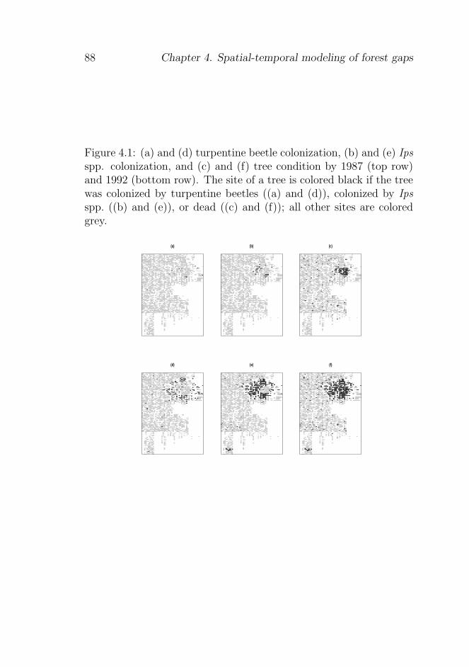
88 Chapter 4. Spatial-temporal modeling of forest gaps
Figure 4.1: (a) and (d) turpentine beetle colonization, (b) and (e) Ipsspp. colonization, and (c) and (f) tree condition by 1987 (top row)and 1992 (bottom row). The site of a tree is colored black if the treewas colonized by turpentine beetles ((a) and (d)), colonized by Ipsspp. ((b) and (e)), or dead ((c) and (f)); all other sites are coloredgrey.
(a)
(d)
(b)
(e)
(c)
(f)
4.3. Observation model 89
spp. colonization took place during year t at site i, i.e. ut,i = 1 ifyt,i = 1 and ut,i = 0 otherwise. In consistency with the data, weassume that Ips spp. colonization could only occur once at a givensite and after colonization of a tree, Ips spp. leaves the tree before theend of the flight season of the same year (before the annual survey).Thus ut,i = 1 for at most one year t. Finally, let zt,i denote the treecondition variable such that zt,i = 0 if the tree was alive and zt,i = 1if the tree was dead at time t and site i.
We let xt = (xt,1, . . . , xt,2715), yt = (yt,1, . . . , yt,2715), and zt =(zt,1, . . . , zt,2715) denote the vectors of respectively the turpentine bee-tle colonization variables, the Ips spp. colonization variables, andthe tree condition variables at time t and all the sites. Further, letut = (ut,1, . . . , ut,2715) and wt = (xt, yt, zt). Since turpentine beetlecolonization typically precedes Ips spp. colonization, which in turnprecedes the death of a tree, we order the variables xt, yt, zt such thatxt precedes yt and yt precedes zt. Thus, the data under study areordered as (z−1, x0, y0, z0, . . . , x5, y5, z5), while the unobserved datain the past are ordered as (. . . , x−2, y−2, z−2, x−1, y−1).
4.3.2 Temporal model
In Sections 4.3.3–4.3.5, we shall construct a set of spatial-temporalmodels to capture the relations among the variables xt,i, yt,i, andzt,i, while accounting for spatial and temporal dependence. Beforespecifying these details, it is useful to give a brief description of thetemporal process wt and how the likelihood factorizes.
In equations (4.1)–(4.3) below we naturally consider a sequen-tial model construction such that for each time t, we specify theconditional distribution of xt first, yt second, zt third given the rel-evant past. The detailed model descriptions (4.5), (4.8), and (4.12)in Sections 4.3.3–4.3.5 imply the following conditional independencestructure for the temporal process. Let [a|b] denote the conditionaldistribution of a random component a given another random com-ponent b. For the turpentine beetle colonization variables at time
90 Chapter 4. Spatial-temporal modeling of forest gaps
t,[xt|(ws)s=t−1,t−2,...] ∼ [xt|xt−1, zt−1] (4.1)
depends on a parameter θ as specified in Section 4.3.3; for the Ipsspp. beetle colonization variables at time t,
[yt|xt, (ws)s=t−1,t−2,...] ∼ [yt|xt, yt−1, zt−1] (4.2)
depends on a parameter ψ (Section 4.3.4); for the tree conditionvariables at time t,
[zt|xt, yt, (ws)s=t−1,t−2,...] ∼ [zt|xt, yt, zt−1] (4.3)
depends on a parameter ϕ (Section 4.3.5). For the correspondinglikelihood terms, we write L(1)(θ) = L(1)(θ;xt|xt−1, zt−1), L
(2)(ψ) =L(2)(ψ; yt|xt, yt−1, zt−1), and L(3)(ϕ) = L(3)(ϕ; zt|xt, yt, zt−1).
For statistical inference we condition on
e = (z−1, x0, y0)
since by (4.1)–(4.3), the remaining data
d = (z0, x1, y1, z1, . . . , x5, y5, z5)
are conditionally independent of the unobserved (. . . , x−2, y−2, z−2,x−1, y−1). We let L(θ, ψ, ϕ) = L(θ, ψ, ϕ; d|e) denote the likelihoodbased on the conditional distribution of d given e. By (4.1)–(4.3),this factorizes into
L(θ, ψ, ϕ; d|e) = L(1)(θ)L(2)(ψ)L(3)(ϕ)
given by the likelihood terms for each type of data
L(1)(θ) =5∏
t=1
L(1)t (θ), L(2)(ϕ) =
5∏
t=1
L(2)t (ϕ), L(3)(ψ) =
5∏
t=0
L(3)t (ψ), (4.4)
where L(1)t (θ)=L
(1)t (θ;xt|xt−1, zt−1), L
(2)t (ψ)=L
(2)t (ψ; yt|xt, yt−1, zt−1),
and L(3)t (ϕ) = L
(3)t (ϕ; zt|xt, yt, zt−1) are specified at the end of Sec-
tions 4.3.3–4.3.5.
4.3. Observation model 91
In Sections 4.3.3–4.3.5, our strategy is for each time, site, andtype of data xt,i, yt,i, or zt,i to specify a “local characteristic” whichonly depends on “local information”. For example, by the local char-acteristic of yt,i, we mean the conditional distribution of yt,i given theother yt,j, j 6= i and the previous history xt, (ws)s=t−1,t−2,.... We ex-press the local information with respect to the grid of tree locationsand consider for site i its first-, second-, . . . order neighbors whichare the (up to) four nearest, four second nearest, . . . sites to i.
4.3.3 Likelihood based on turpentine beetle col-
onization
The cumulative number of turpentine beetles at time t and site i isassumed to depend on local information such that
[xt,i|(xt,j)j 6=i, (ws)s=t−1,t−2,...] ∼[
xt,i|xt−1,Nxi, zt−1,i
]
(4.5)
where xt−1,Nxi
is the vector of variables xj with j ∈ Nxi . Here Nx
i
consists of i and its neighbors up to the fifth order, and we assumethat the conditional distribution of turpentine beetle colonization attime t depends only on turpentine beetle colonization at time t − 1and at sites in Nx
i , since this neighborhood is fairly large but is stillinterpretable biologically (see Section 4.5 for further details). Sinceturpentine beetles colonize red pines during only one brief period peryear, and a tree can be colonized by multiple turpentine beetles, weassume conditional independence among nearby sites within the sameyear. On the other hand, turpentine beetles that colonize a tree inone spring tend to colonize nearby trees in the next spring. Thus webuild into the model a possible relation between turpentine beetlecolonization at time t and at time t− 1.
The local characteristic [xt,i|xt−1,Nxi, zt−1,i] is specified as follows.
If the tree at site i was dead at time t − 1 (i.e. zt−1,i = 1), the lo-cal characteristic is deterministic with xt,i = xt−1,i, since turpentinebeetles will not colonize a dead tree. Turpentine beetles could the-oretically colonize a tree that dies from competitive thinning, i.e., a
92 Chapter 4. Spatial-temporal modeling of forest gaps
process in which the growth of neighboring trees blocks out neces-sary sunlight. However, such events were rare in the stand, as theinsects would likely colonize the weakened tree in advance of treedeath. Moreover, the diameter and subcortical tissues of trees thathave been crowded to death are frequently too thin to serve as asuitable breeding substrate for this insect. Turpentine beetles couldalso colonize a healthy tree that was killed suddenly, such as by alightning strike or during a wind storm. However, we did not findany visual evidence of lightning (e.g., shredded bark, burn marks,or shattered limbs) or windthrow (other than trees that had alreadybeen killed) in any of our annual surveys. Hence, focusing on thecolonization of live trees, if the tree at site i was alive at time t − 1(i.e. zt−1,i = 0), we assume that
[
xt,i − xt−1,i|xt−1,Nxi, zt−1,i = 0
]
∼ Poisson(λt,i)
where
log(λt,i) = θ0 + θ1
∑
j∈Nxi
xt−1,j. (4.6)
Thus, given the past, the xt,i − xt−1,i with zt−1,i = 0 form a samplefrom a Poisson regression, so
L(1)t (θ) ∝
∏
i:zt−1,i=0
λxt,i−xt−1,i
t,i exp(−λt,i)
= exp
∑
i:zt−1,i=0
[
(xt,i − xt−1,i)
(
θ0 + θ1
∑
j∈Nxi
xt−1,j
)
− exp
(
θ0 + θ1
∑
j∈Nxi
xt−1,j
)]
. (4.7)
4.3. Observation model 93
4.3.4 Likelihood based on Ips spp. colonization
The conditional dependence structure for whether colonization by Ipsbeetles has occurred is assumed to be
[yt,i|xt, (yt,j)j 6=i, (ws)s=t−1,t−2,...]
∼ [yt,i|xt,i, ut,Nyi, ut−1,N
yi, yt−1,i, zt−1,i]. (4.8)
Thus we assume that the conditional distribution of Ips spp. colo-nization at time t depends on turpentine beetle colonization at timet, Ips spp. colonization at sites j ∈ N y
i at both time t−1 and t, whereN y
i consists of the first and second order neighbors to i (note that N yi
does not include i). Since it is hypothesized that turpentine beetlespredispose red pines to colonization by Ips spp., we include in themodel a possible relation to the number of turpentine beetle pitchtubes on the tree. Since Ips spp. attack different red pines 1–3 timesper year and can overwinter near the trees they have colonized, we as-sume relations among neighboring sites for both time t and t− 1 andthat a first- and second-order neighborhood would suffice to capturespatial dependence in this study.
The local characteristic [yt,i|xt,i, ut,Nyi, ut−1,N
yi, yt−1,i, zt−1,i] is spec-
ified as follows. If the tree at site i was dead at time t − 1 (i.e.zt−1,i = 1) or was colonized by Ips spp. at previous times (i.e.,yt−1,i = 1 or 2), the local characteristic is deterministic with yt,i = 0or 2, since Ips spp. will not colonize a dead tree. Ips spp. could the-oretically colonize a tree that dies from competitive thinning, i.e.,overshadowing and crowding by more dominant neighbors, althoughin practice the insects would likely find and colonize a weakened treein advance of tree death, and would colonize only if the subcorticaltissue was sufficiently thick. Such trees also contribute little to theecological dynamics of the system, as they are commonly colonized bycompeting species of insects against which Ips spp. fare poorly. Wealso disregard the possibility that Ips spp. colonize lightning strikesor recent windthrow of live trees, due to the absence of such eventsobserved during our annual surveys. Hence, focusing on colonization
94 Chapter 4. Spatial-temporal modeling of forest gaps
of live trees, if the tree at site i was alive at time t−1 (i.e. zt−1,i = 0)and was not colonized previously (yt,i = 0), the local characteristic isassumed to be a logistic regression,
[
yt,i|xt,i, ut,Nyi, ut−1,N
yi, yt−1,i = 0, zt−1,i = 0
]
∼ Bernoulli(pt,i) (4.9)
where
logit(pt,i) = ψ0 + ψ1xt,i + ψ2
∑
j∈Nyi
ut−1,j + ψ3
∑
j∈Nyi
ut,j. (4.10)
Since ut,i = yt,i in (4.9), by the Hammersley-Clifford theorem, L(2)t (ψ)
is equal to
exp
∑
i:yt−1,i=zt−1,i=0
ψ0 + ψ1xt,i + ψ2
∑
j∈Nyi
ut−1,j
ut,i
+ψ3
∑
i<j: j∈Nyi
ut,iut,j
/
c(xt, yt−1, zt−1, ψ) (4.11)
where c(xt, yt−1, zt−1, ψ) is a normalizing constant (note that j ∈N y
i ⇔ i ∈ N yj ). In other words, given the past, the ut,i with yt,i =
zt,i = 0 form an autologistic model (Besag, 1974).
4.3.5 Likelihood based on tree condition
The conditional dependence structure for tree condition is assumedto be
[zt,i|xt, yt, (zt,j)j 6=i, (ws)s=t−1,t−2,...] ∼ [zt,i|xt,i, ut,i, zt−1,Nzi, zt−1,i] (4.12)
where the neighborhood N zi consists of the neighbors up to the fifth
order. If the tree at site i was dead at time t − 1 (i.e. zt−1,i = 1),the local characteristic is deterministic with zt,i = 1, because a dead
4.4. Bayesian model and posterior simulations 95
tree remains dead. But if the tree at site i was alive at time t − 1(i.e. zt−1,i = 0), the local characteristic is assumed to be a logisticregression,
[
zt,i|xt,i, ut,i, zt−1,Nzi, zt−1,i = 0
]
∼ Bernoulli(qt,i)
where
logit(qt,i) = ϕ0 + ϕ1xt,i + ϕ2ut,i + ϕ3
∑
j∈Nzi
zt−1,j. (4.13)
That is, mortality rate of a tree depends on both turpentine beetlecolonization and Ips spp. colonization. The additional term involvingthe tree condition at time t−1 is a way of accounting for any potentialspatial dependence. Again we consider a fairly large neighborhoodthat consists of neighbors up to the fifth order. Conditional on thepast, the zt,i with zt−1,i = 0 form a sample from a logistic regressions,so
L(3)t (ϕ) =
∏
i:zt−1,i=0
exp(zt,ilogit(qt,i))
1 + exp(logit(qt,i))
=∏
i:zt−1,i=0
exp(zt,i(ϕ0 + ϕ1xt,i + ϕ2ut,i + ϕ3
∑
j∈Nzizt−1,j))
1 + exp(ϕ0 + ϕ1xt,i + ϕ2ut,i + ϕ3
∑
j∈Nzizt−1,j)
.
(4.14)
4.4 Bayesian model and posterior simu-
lations
We assume independent improper uniform priors
p(θ) ∝ 1, θ ∈ R2; p(ψ) ∝ 1, ψ ∈ R
4; p(ϕ) ∝ 1, ϕ ∈ R4.
Thus θ, ψ, ϕ are a posteriori independent with densities
π(θ) ∝ L(1)(θ), θ ∈ R2; π(ψ) ∝ L(2)(ψ), ψ ∈ R
4;
π(ϕ) ∝ L(3)(ϕ), ϕ ∈ R4. (4.15)
96 Chapter 4. Spatial-temporal modeling of forest gaps
For a discussion of posterior properity, see Appendix A. For the re-maining discussion of MCMC simulations, we assume the reader isfamiliar with MCMC methods (e.g. Robert and Casella (2004)).
For turpentine beetles, we will simulate from the marginal pos-terior distribution of θ using a Metropolis within Gibbs algorithm,where we alternate between updating θ0 and θ1. Since the full condi-tional for λ0 = exp(θ0) is a Gamma distribution with shape parameter∑
t,i(xt,i−xt−1,i) and inverse scale parameter∑
t,i exp(θ1
∑
j∈Nxixt−1,j),
where in both cases the sum∑
t,i is over those t, i with zt−1,i = yt−1,i =0, we use a Gibbs update for this component. The full conditionalfor the other parameter θ1 is not a standard distribution, so herewe use a Metropolis random walk algorithm with a normal proposaldistribution, cf. Robert and Casella (2004).
For Ips spp., suppose we use a Metropolis-Hastings algorithm tosimulate from the marginal posterior distribution of ψ. Let L
(2)unnorm(ψ;u)
denote L(2) in (4.4) but without the unknown normalizing constant
c(ψ) =5∏
t=1
c(xt, yt−1, zt−1, ψ)
from (4.11); here u denotes the vector of all observed ut,i values.If ψ is the current and ψ′ is the proposed parameter values in theMetropolis-Hastings algorithm, then the Hastings ratio depends onthe ratio c(ψ′)/c(ψ) of unknown normalizing constants. This can beapproximated by path sampling (e.g. Gelman and Meng (1998)),
logc(ψ′)
c(ψ)≈
1
n
n∑
k=1
[
d
dslogL(2)
unnorm(ψ(sk); υk)
]
. (4.16)
Here we let s1, . . . , sn be independent and uniformly distributed on[0, 1], and ψ(s) = sψ′ + (1 − s)ψ, 0 ≤ s ≤ 1 is a line segment.Further, each υk is a perfect simulation of u = (u1, . . . , u5) where ut
given the past follows the autologistic model (4.11) with parameterψ(sk) (Propp and Wilson, 1996; Møller, 1999). Furthermore, givens1, . . . , sn, the perfect simulations υ1, . . . , υn are independent.
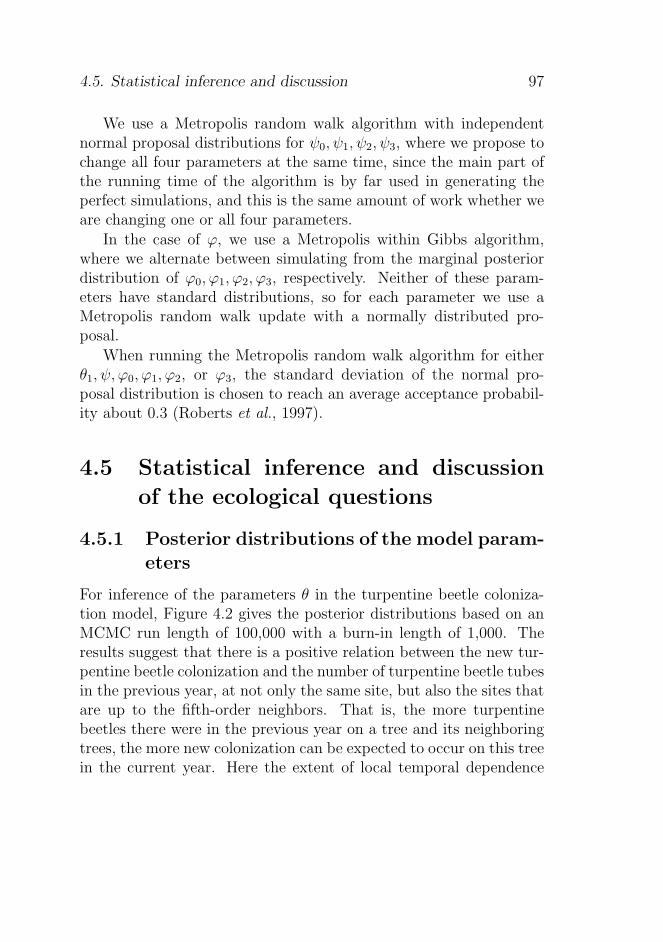
4.5. Statistical inference and discussion 97
We use a Metropolis random walk algorithm with independentnormal proposal distributions for ψ0, ψ1, ψ2, ψ3, where we propose tochange all four parameters at the same time, since the main part ofthe running time of the algorithm is by far used in generating theperfect simulations, and this is the same amount of work whether weare changing one or all four parameters.
In the case of ϕ, we use a Metropolis within Gibbs algorithm,where we alternate between simulating from the marginal posteriordistribution of ϕ0, ϕ1, ϕ2, ϕ3, respectively. Neither of these param-eters have standard distributions, so for each parameter we use aMetropolis random walk update with a normally distributed pro-posal.
When running the Metropolis random walk algorithm for eitherθ1, ψ, ϕ0, ϕ1, ϕ2, or ϕ3, the standard deviation of the normal pro-posal distribution is chosen to reach an average acceptance probabil-ity about 0.3 (Roberts et al., 1997).
4.5 Statistical inference and discussion
of the ecological questions
4.5.1 Posterior distributions of the model param-
eters
For inference of the parameters θ in the turpentine beetle coloniza-tion model, Figure 4.2 gives the posterior distributions based on anMCMC run length of 100,000 with a burn-in length of 1,000. Theresults suggest that there is a positive relation between the new tur-pentine beetle colonization and the number of turpentine beetle tubesin the previous year, at not only the same site, but also the sites thatare up to the fifth-order neighbors. That is, the more turpentinebeetles there were in the previous year on a tree and its neighboringtrees, the more new colonization can be expected to occur on this treein the current year. Here the extent of local temporal dependence
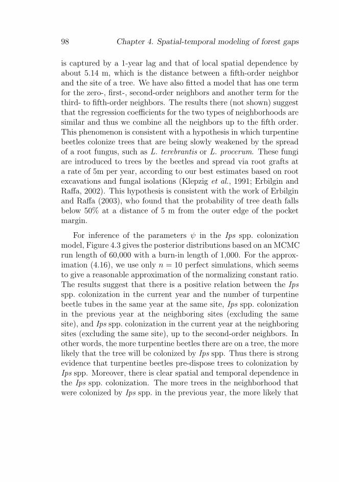
98 Chapter 4. Spatial-temporal modeling of forest gaps
is captured by a 1-year lag and that of local spatial dependence byabout 5.14 m, which is the distance between a fifth-order neighborand the site of a tree. We have also fitted a model that has one termfor the zero-, first-, second-order neighbors and another term for thethird- to fifth-order neighbors. The results there (not shown) suggestthat the regression coefficients for the two types of neighborhoods aresimilar and thus we combine all the neighbors up to the fifth order.This phenomenon is consistent with a hypothesis in which turpentinebeetles colonize trees that are being slowly weakened by the spreadof a root fungus, such as L. terebrantis or L. procerum. These fungiare introduced to trees by the beetles and spread via root grafts ata rate of 5m per year, according to our best estimates based on rootexcavations and fungal isolations (Klepzig et al., 1991; Erbilgin andRaffa, 2002). This hypothesis is consistent with the work of Erbilginand Raffa (2003), who found that the probability of tree death fallsbelow 50% at a distance of 5 m from the outer edge of the pocketmargin.
For inference of the parameters ψ in the Ips spp. colonizationmodel, Figure 4.3 gives the posterior distributions based on an MCMCrun length of 60,000 with a burn-in length of 1,000. For the approx-imation (4.16), we use only n = 10 perfect simulations, which seemsto give a reasonable approximation of the normalizing constant ratio.The results suggest that there is a positive relation between the Ipsspp. colonization in the current year and the number of turpentinebeetle tubes in the same year at the same site, Ips spp. colonizationin the previous year at the neighboring sites (excluding the samesite), and Ips spp. colonization in the current year at the neighboringsites (excluding the same site), up to the second-order neighbors. Inother words, the more turpentine beetles there are on a tree, the morelikely that the tree will be colonized by Ips spp. Thus there is strongevidence that turpentine beetles pre-dispose trees to colonization byIps spp. Moreover, there is clear spatial and temporal dependence inthe Ips spp. colonization. The more trees in the neighborhood thatwere colonized by Ips spp. in the previous year, the more likely that
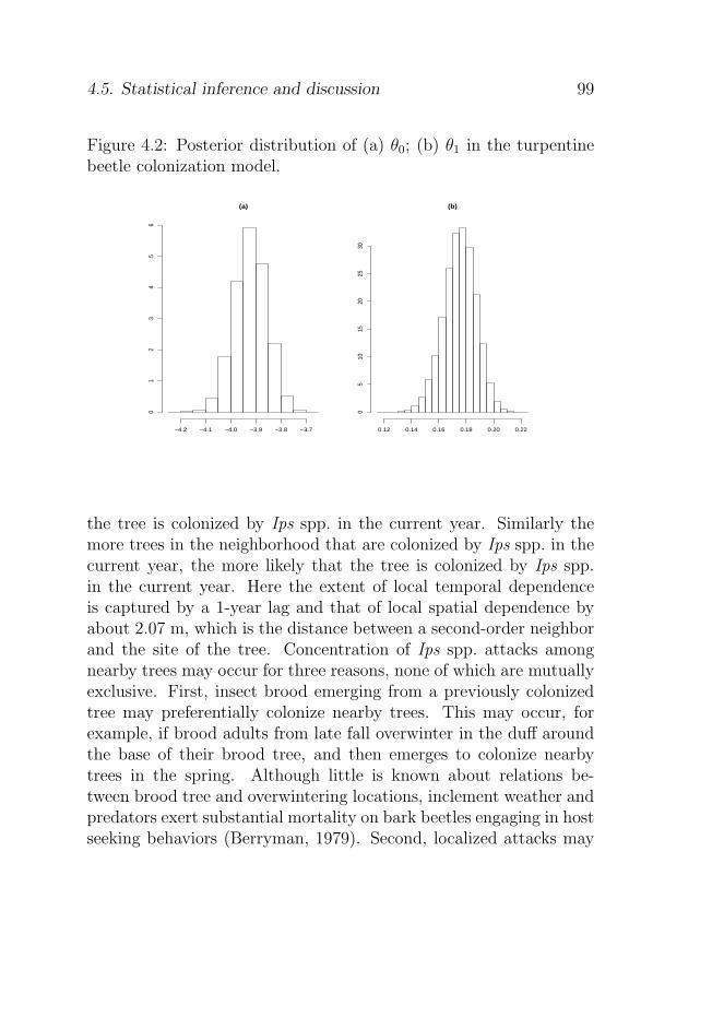
4.5. Statistical inference and discussion 99
Figure 4.2: Posterior distribution of (a) θ0; (b) θ1 in the turpentinebeetle colonization model.
(a)
−4.2 −4.1 −4.0 −3.9 −3.8 −3.7
01
23
45
6
(b)
0.12 0.14 0.16 0.18 0.20 0.22
05
1015
2025
30
the tree is colonized by Ips spp. in the current year. Similarly themore trees in the neighborhood that are colonized by Ips spp. in thecurrent year, the more likely that the tree is colonized by Ips spp.in the current year. Here the extent of local temporal dependenceis captured by a 1-year lag and that of local spatial dependence byabout 2.07 m, which is the distance between a second-order neighborand the site of the tree. Concentration of Ips spp. attacks amongnearby trees may occur for three reasons, none of which are mutuallyexclusive. First, insect brood emerging from a previously colonizedtree may preferentially colonize nearby trees. This may occur, forexample, if brood adults from late fall overwinter in the duff aroundthe base of their brood tree, and then emerges to colonize nearbytrees in the spring. Although little is known about relations be-tween brood tree and overwintering locations, inclement weather andpredators exert substantial mortality on bark beetles engaging in hostseeking behaviors (Berryman, 1979). Second, localized attacks may
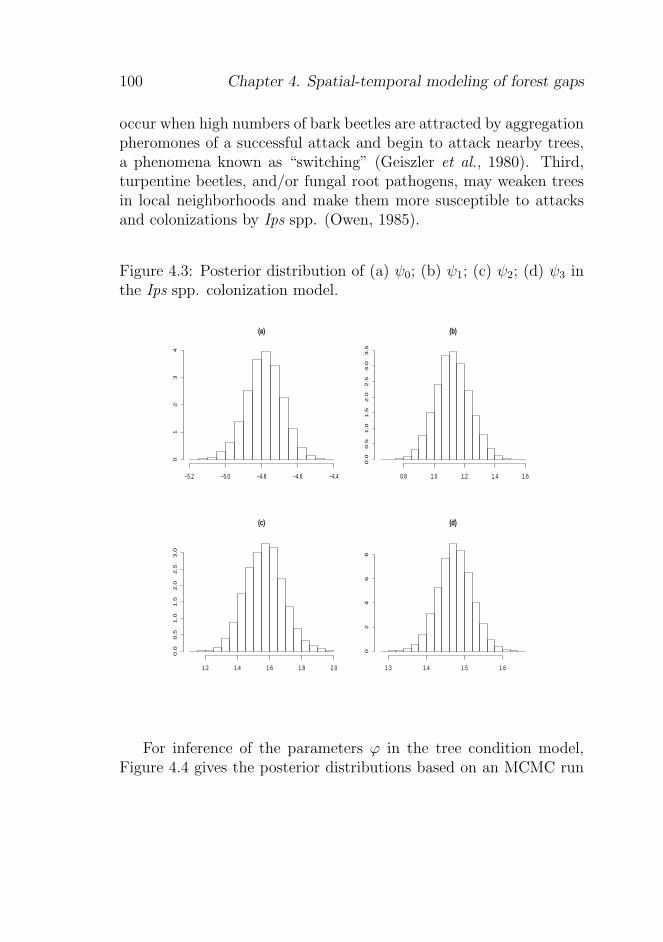
100 Chapter 4. Spatial-temporal modeling of forest gaps
occur when high numbers of bark beetles are attracted by aggregationpheromones of a successful attack and begin to attack nearby trees,a phenomena known as “switching” (Geiszler et al., 1980). Third,turpentine beetles, and/or fungal root pathogens, may weaken treesin local neighborhoods and make them more susceptible to attacksand colonizations by Ips spp. (Owen, 1985).
Figure 4.3: Posterior distribution of (a) ψ0; (b) ψ1; (c) ψ2; (d) ψ3 inthe Ips spp. colonization model.
(a)
−5.2 −5.0 −4.8 −4.6 −4.4
01
23
4
(b)
0.8 1.0 1.2 1.4 1.6
0.0
0.5
1.0
1.5
2.0
2.5
3.0
3.5
(c)
1.2 1.4 1.6 1.8 2.0
0.0
0.5
1.0
1.5
2.0
2.5
3.0
(d)
1.3 1.4 1.5 1.6
02
46
8
For inference of the parameters ϕ in the tree condition model,Figure 4.4 gives the posterior distributions based on an MCMC run

4.5. Statistical inference and discussion 101
length of 100,000 with a burn-in length of 1,000. The results sug-gest that there is no evidence of a direct relation between a tree’scondition and the number of its turpentine beetle tubes, but thereis a strong positive relation between Ips spp. colonization and sub-sequent tree death. That is, the number of turpentine beetles doesnot directly influence the mortality of tree, but there is a very largeincrease in the probability that a tree dies after colonized by Ipsspp. in the same year. This is not surprising, as trees may survivecolonization of the root collar by turpentine beetles for more thanone year. However, Ips spp. utilize aggregation pheromones to at-tract high numbers of conspecifics that quickly colonize all availablesubcortical tissue. The water-conducting tissues are mined by thedeveloping larvae, and the tree dies soon thereafter. Furthermoreit appears necessary to account for the spatial-temporal dependenceamong the tree conditions.
4.5.2 Empirical and predictive rates of mortality
and Ips spp. colonization
In this and the next subsection we check important aspects of themodel that correspond to the ecological questions of interest, particu-larly the relations among turpentine beetle colonization, Ips spp. colo-nization, and tree conditions (see Section 4.1). The model checking isbased on posterior predictive distributions obtained by a Monte Carlosample (x(s), u(s), z(s)), s = 1, . . . , S where the Monte Carlo samplesize is chosen to be S = 100. More precisely, since inference is per-formed conditional on e, given a posterior simulation (θ(s), ψ(s), ϕ(s)),we simulate “new data” (x(s), u(s), z(s)) from the conditional distribu-tion of d given e as specified in Section 4.3. This is done using thesequential model construction in Section 4.3, where simulation of xt
and zt given their relevant past is straightforward (see Sections 4.3.3and 4.3.5), while we use perfect simulation for yt given the relevant
past (see Section 4.3.4). Note that x(s)0 = x0, y
(s)0 = y0, and z
(s)−1 = z−1.
The samples (θ(s), ψ(s), ϕ(s)), s = 1, . . . , S are chosen such that they
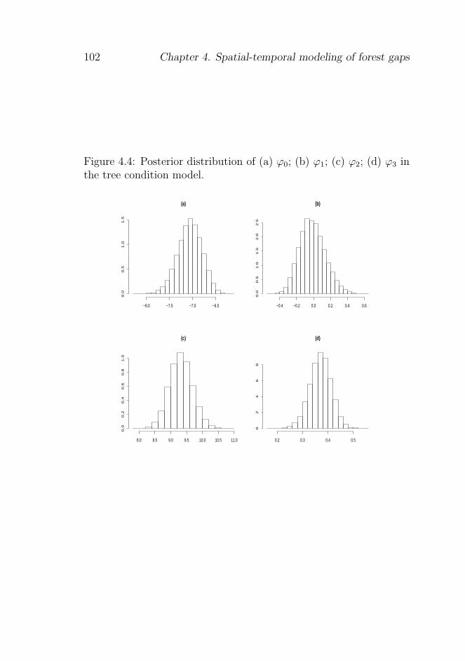
102 Chapter 4. Spatial-temporal modeling of forest gaps
Figure 4.4: Posterior distribution of (a) ϕ0; (b) ϕ1; (c) ϕ2; (d) ϕ3 inthe tree condition model.
(a)
−8.0 −7.5 −7.0 −6.5
0.0
0.5
1.0
1.5
(b)
−0.4 −0.2 0.0 0.2 0.4 0.6
0.0
0.5
1.0
1.5
2.0
2.5
(c)
8.0 8.5 9.0 9.5 10.0 10.5 11.0
0.0
0.2
0.4
0.6
0.8
1.0
(d)
0.2 0.3 0.4 0.5
02
46
8
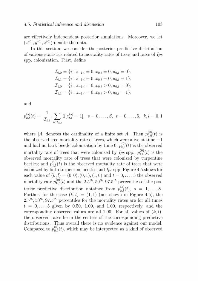
4.5. Statistical inference and discussion 103
are effectively independent posterior simulations. Moreover, we let(x(0), y(0), z(0)) denote the data.
In this section, we consider the posterior predictive distributionof various statistics related to mortality rates of trees and rates of Ipsspp. colonization. First, define
I0,0 = {i : z−1,i = 0, x0,i = 0, u0,i = 0},
I0,1 = {i : z−1,i = 0, x0,i = 0, u0,i = 1},
I1,0 = {i : z−1,i = 0, x0,i > 0, u0,i = 0},
I1,1 = {i : z−1,i = 0, x0,i > 0, u0,i = 1},
and
p(s)k,l (t) =
1
|Ik,l|
∑
i∈Ik,l
1[z(s)t,i = 1], s = 0, . . . , S, t = 0, . . . , 5, k, l = 0, 1
where |A| denotes the cardinality of a finite set A. Then p(0)0,0(t) is
the observed tree mortality rate of trees, which were alive at time −1and had no bark beetle colonization by time 0; p
(0)0,1(t) is the observed
mortality rate of trees that were colonized by Ips spp.; p(0)1,0(t) is the
observed mortality rate of trees that were colonized by turpentinebeetles; and p
(0)1,1(t) is the observed mortality rate of trees that were
colonized by both turpentine beetles and Ips spp. Figure 4.5 shows foreach value of (k, l) = (0, 0), (0, 1), (1, 0) and t = 0, . . . , 5 the observed
mortality rate p(0)k,l (t) and the 2.5th, 50th, 97.5th percentiles of the pos-
terior predictive distribution obtained from p(s)k,l (t), s = 1, . . . , S.
Further, for the case (k, l) = (1, 1) (not shown in Figure 4.5), the2.5th, 50th, 97.5th percentiles for the mortality rates are for all timest = 0, . . . , 5 given by 0.50, 1.00, and 1.00, respectively, and thecorresponding observed values are all 1.00. For all values of (k, l),the observed rates lie in the centers of the corresponding predictivedistributions. Thus overall there is no evidence against our model.Compared to p
(0)0,0(t), which may be interpreted as a kind of observed

104 Chapter 4. Spatial-temporal modeling of forest gaps
baseline mortality rate, p(0)0,1(t) increased greatly and the large in-
crease occurred within the same year of Ips spp. colonization; p(0)1,0(t)
increased at time 1 and the increase leveled off at time 2; and p(0)1,1(t)
is nearly 100% within the same year of the colonization. The pre-dictive distributions show a similar behavior. The fact that deathsof trees occur in both the first and the second year after turpentinebeetle colonization gives further evidence that turpentine beetles pre-dispose a tree to death rather than killing a tree directly. The resulthere also supports the theory that Ips spp., unlike turpentine beetles,are the ultimate mortality agents of red pines.
Figure 4.5: Central 95% prediction intervals and medians (indicatedby bars) for the tree mortality rates over time t = 0, . . . , 5 amongthose trees that were alive at t = −1 and, (a) were not colonized(xi,0 = ui,0 = 0), (b) were colonized by turpentine beetles (xi,0 >0, ui,0 = 0), and (c) were colonized by Ips spp. (xi,0 = 0, ui,0 = 1) att = 0. The corresponding observed tree mortality rates are indicatedby crosses. Note the different scales on the y-axes.
0 1 2 3 4 5
0.00
0.05
0.10
0.15
0.20
(a)
0 1 2 3 4 5
0.0
0.2
0.4
0.6
0.8
1.0
(b)
0 1 2 3 4 5
0.80
0.85
0.90
0.95
1.00
(c)
Next, let
Ik = {i : z−1,i = 0, x0,i = k}, k = 0, 1,
denote the collection of sites where a tree was alive at time −1 andwas (k = 1) or was not (k = 0) colonized by turpentine beetles by
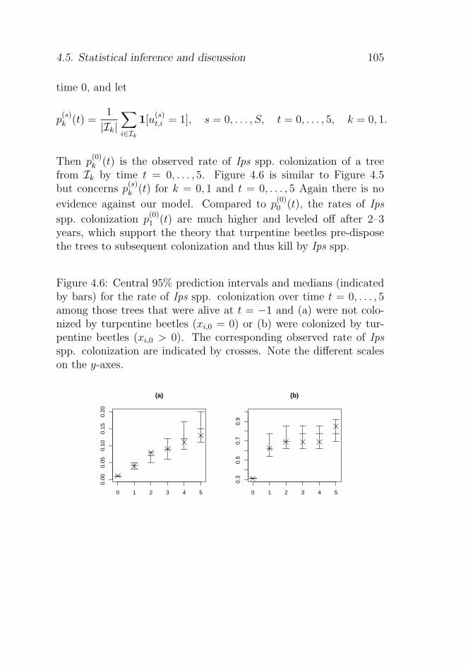
4.5. Statistical inference and discussion 105
time 0, and let
p(s)k (t) =
1
|Ik|
∑
i∈Ik
1[u(s)t,i = 1], s = 0, . . . , S, t = 0, . . . , 5, k = 0, 1.
Then p(0)k (t) is the observed rate of Ips spp. colonization of a tree
from Ik by time t = 0, . . . , 5. Figure 4.6 is similar to Figure 4.5but concerns p
(s)k (t) for k = 0, 1 and t = 0, . . . , 5 Again there is no
evidence against our model. Compared to p(0)0 (t), the rates of Ips
spp. colonization p(0)1 (t) are much higher and leveled off after 2–3
years, which support the theory that turpentine beetles pre-disposethe trees to subsequent colonization and thus kill by Ips spp.
Figure 4.6: Central 95% prediction intervals and medians (indicatedby bars) for the rate of Ips spp. colonization over time t = 0, . . . , 5among those trees that were alive at t = −1 and (a) were not colo-nized by turpentine beetles (xi,0 = 0) or (b) were colonized by tur-pentine beetles (xi,0 > 0). The corresponding observed rate of Ipsspp. colonization are indicated by crosses. Note the different scaleson the y-axes.
0 1 2 3 4 5
0.00
0.05
0.10
0.15
0.20
(a)
0 1 2 3 4 5
0.3
0.5
0.7
0.9
(b)

106 Chapter 4. Spatial-temporal modeling of forest gaps
4.5.3 Checking further aspects of the model
To check whether the model captures the relation between turpentinebeetle colonization and Ips spp. colonization and between coloniza-tion of Ips spp. and tree mortality, we consider
r(s)x,u =
5∑
t=1
∑
i
(x(s)t,i − x
(s)t−1,i)u
(s)t,i , r(s)
u,z =5∑
t=1
∑
i
u(s)t,i z
(s)t,i , s = 0, . . . , S.
Here r(0)x,u summarizes the observed relation between new colonization
of turpentine beetles and new colonization of Ips spp. in the sameyear and at the same site, and r
(0)u,z summarizes the observed occur-
rences of Ips spp. colonization that is involved in mortality of trees.Furthermore, for spatial dependence structure, we consider
v(s)x,x(δ) =
∑
i,j:d(i,j)∈N(δ)
1[x(s)5,i > 0, x
(s)5,j > 0], s = 0, . . . , S, δ > 0,
v(s)y,y(δ) =
∑
i,j:d(i,j)∈N(δ)
1[y(s)5,i > 0, y
(s)5,j > 0], s = 0, . . . , S, δ > 0,
v(s)z,z(δ) =
∑
i,j:d(i,j)∈N(δ)
1[z(s)5,i = 1, z
(s)5,j = 1], s = 0, . . . , S, δ > 0,
where d(i, j) denotes the Euclidean distance between sites i and
j, and N(δ) = (δ − 1, δ] is a half-open interval. That is, v(0)x,x(δ)
(v(0)y,y(δ), v
(0)z,z(δ)) captures the observed spatial relation between tur-
pentine beetle colonization (Ips spp. colonization, tree mortality) attwo sites that are at least δ−1 and at most δ apart in distance. Herewe focus on cumulative effect of all three variables for simplicity.
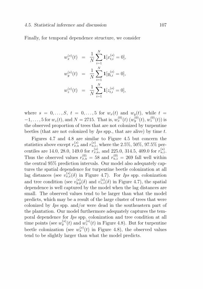
4.5. Statistical inference and discussion 107
Finally, for temporal dependence structure, we consider
w(s)x (t) =
1
N
N∑
i=1
1[x(s)t,i = 0],
w(s)y (t) =
1
N
N∑
i=1
1[y(s)t,i = 0],
w(s)z (t) =
1
N
N∑
i=1
1[z(s)t,i = 0],
where s = 0, . . . , S, t = 0, . . . , 5 for wx(t) and wy(t), while t =
−1, . . . , 5 for wz(t), andN = 2715. That is, w(0)x (t) (w
(0)y (t), w
(0)z (t)) is
the observed proportion of trees that are not colonized by turpentinebeetles (that are not colonized by Ips spp., that are alive) by time t.
Figures 4.7 and 4.8 are similar to Figure 4.5 but concern thestatistics above except r
(s)x,u and r
(s)u,z, where the 2.5%, 50%, 97.5% per-
centiles are 14.0, 28.0, 149.0 for r(s)x,u, and 225.0, 314.5, 409.0 for r
(s)u,z.
Thus the observed values r(0)x,u = 58 and r
(0)u,z = 269 fall well within
the central 95% prediction intervals. Our model also adequately cap-tures the spatial dependence for turpentine beetle colonization at alllag distances (see v
(s)x,x(δ) in Figure 4.7). For Ips spp. colonization
and tree condition (see v(s)y,y(δ) and v
(s)z,z(δ) in Figure 4.7), the spatial
dependence is well captured by the model when the lag distances aresmall. The observed values tend to be larger than what the modelpredicts, which may be a result of the large cluster of trees that werecolonized by Ips spp. and/or were dead in the southeastern part ofthe plantation. Our model furthermore adequately captures the tem-poral dependence for Ips spp. colonization and tree condition at alltime points (see w
(s)y (t) and w
(s)z (t) in Figure 4.8). But for turpentine
beetle colonization (see w(s)x (t) in Figure 4.8), the observed values
tend to be slightly larger than what the model predicts.
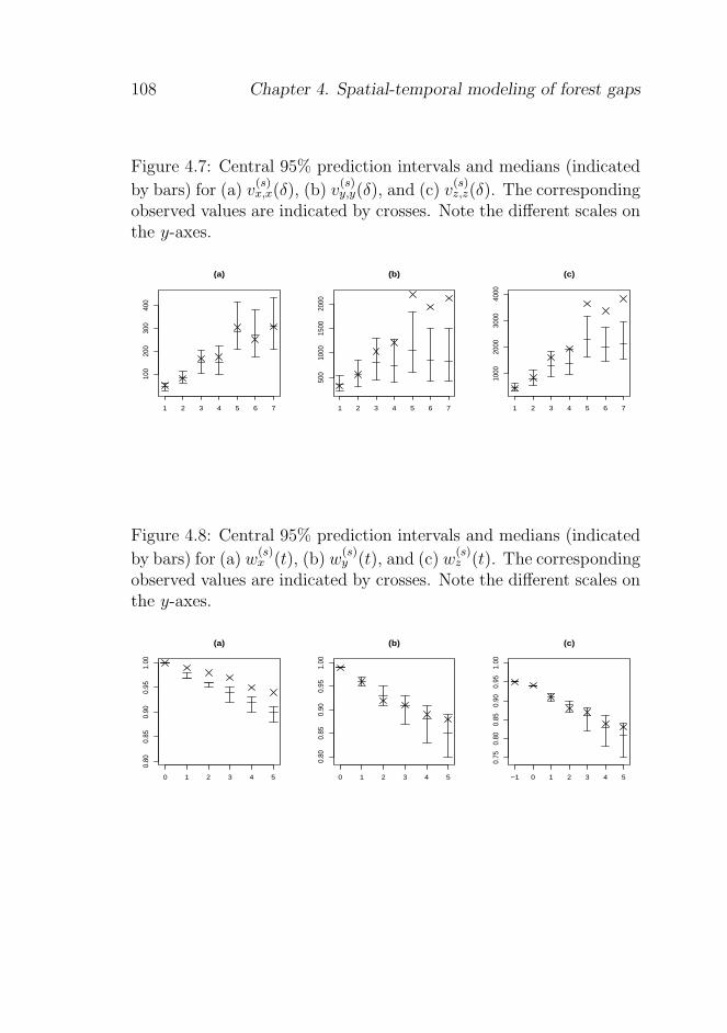
108 Chapter 4. Spatial-temporal modeling of forest gaps
Figure 4.7: Central 95% prediction intervals and medians (indicated
by bars) for (a) v(s)x,x(δ), (b) v
(s)y,y(δ), and (c) v
(s)z,z(δ). The corresponding
observed values are indicated by crosses. Note the different scales onthe y-axes.
1 2 3 4 5 6 7
100
200
300
400
(a)
1 2 3 4 5 6 7
500
1000
1500
2000
(b)
1 2 3 4 5 6 7
1000
2000
3000
4000
(c)
Figure 4.8: Central 95% prediction intervals and medians (indicated
by bars) for (a) w(s)x (t), (b) w
(s)y (t), and (c) w
(s)z (t). The corresponding
observed values are indicated by crosses. Note the different scales onthe y-axes.
0 1 2 3 4 5
0.80
0.85
0.90
0.95
1.00
(a)
0 1 2 3 4 5
0.80
0.85
0.90
0.95
1.00
(b)
−1 0 1 2 3 4 5
0.75
0.80
0.85
0.90
0.95
1.00
(c)
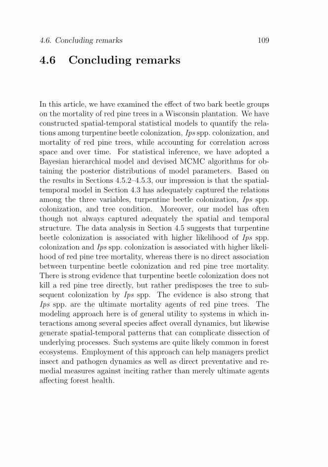
4.6. Concluding remarks 109
4.6 Concluding remarks
In this article, we have examined the effect of two bark beetle groupson the mortality of red pine trees in a Wisconsin plantation. We haveconstructed spatial-temporal statistical models to quantify the rela-tions among turpentine beetle colonization, Ips spp. colonization, andmortality of red pine trees, while accounting for correlation acrossspace and over time. For statistical inference, we have adopted aBayesian hierarchical model and devised MCMC algorithms for ob-taining the posterior distributions of model parameters. Based onthe results in Sections 4.5.2–4.5.3, our impression is that the spatial-temporal model in Section 4.3 has adequately captured the relationsamong the three variables, turpentine beetle colonization, Ips spp.colonization, and tree condition. Moreover, our model has oftenthough not always captured adequately the spatial and temporalstructure. The data analysis in Section 4.5 suggests that turpentinebeetle colonization is associated with higher likelihood of Ips spp.colonization and Ips spp. colonization is associated with higher likeli-hood of red pine tree mortality, whereas there is no direct associationbetween turpentine beetle colonization and red pine tree mortality.There is strong evidence that turpentine beetle colonization does notkill a red pine tree directly, but rather predisposes the tree to sub-sequent colonization by Ips spp. The evidence is also strong thatIps spp. are the ultimate mortality agents of red pine trees. Themodeling approach here is of general utility to systems in which in-teractions among several species affect overall dynamics, but likewisegenerate spatial-temporal patterns that can complicate dissection ofunderlying processes. Such systems are quite likely common in forestecosystems. Employment of this approach can help managers predictinsect and pathogen dynamics as well as direct preventative and re-medial measures against inciting rather than merely ultimate agentsaffecting forest health.
110 Chapter 4. Spatial-temporal modeling of forest gaps
Appendix A
From a practical viewpoint, we would expect our MCMC runs to di-verge if an improper posterior distribution had been specified. Froma theoretical viewpoint, since the three likelihood functions in (4.15)are log concave, properity of the posteriors with uniform improperpriors is equivalent to the existence of the maximum likelihood es-timate (MLE) based on L(1)(θ), L(2)(ψ), and L(3)(ϕ), respectively.This can be established as sketched below.
The likelihood functions L(1)(θ), L(2)(ψ), L(3)(ϕ) in (4.7), (4.11),
(4.14) are products of log concave functions L(1)t (θ), L
(2)t (ψ), L
(3)t (ϕ),
respectively. Therefore, to verify the existence of the MLE basedon L(1)(θ), L(2)(ψ), L(3)(ϕ), it suffices for each t = 1, . . . , 5 to verify
the existence of the MLE based on L(1)t (θ), L
(2)t (ψ), L
(3)t (ϕ), respec-
tively. This can easily be checked in the cases of the Poisson regres-sion L
(1)t (θ) based on the data xt and the logistic regression L(3)(ϕ)
based on the data zt, either by theoretical results (Barndorff-Nielsen,1978; Jacobsen, 1989) or using software for generalized linear mod-
els. Moreover, by (4.11), L(2)t (ψ) is of regular exponential family form
with canonical statistic
s(2)t (ut) =
∑
i:yt−1,i=zt−1,i=0
ut,i, xt,iut,i,∑
j∈Nyi
ut−1,jut,i,∑
j: j∈Nyi
ut,iut,j
.
Consequently, by a well-known result from exponential family theory(Barndorff-Nielsen, 1978), the MLE of ψ based on the data ut exists
if s(2)t (ut) belongs to the interior of the convex hull of its support.
This condition seems less straightforward to check, so alternatively,MCMC methods for finding the MLE may be applied (Geyer andThompson, 1992).
4.6. Concluding remarks 111
Acknowledgment
Funding has been provided for this research from NSF: DEB-0314215and the Wisconsin Alumni Research Foundation. We thank the Wis-consin Department of Natural Resources for providing the researchsite.
References
Auclair, A. N. D. (2005). Patterns and general characteristics ofsevere forest dieback from 1950 to 1995 in the northeastern UnitedStates. Canadian Journal of Forest Research, 35, 1342–1355.
Aukema, B. H., Clayton, M. K., and Raffa, K. F. (2005). Modelingflight activity and population dynamics of the pine engraver, Ipspini, in the Great Lakes region: Effects of weather and predatorsat short time scales. Population Ecology , 47, 61–69.
Barndorff-Nielsen, O. E. (1978). Information and Exponential Fam-ilies in Statistical Theory . Wiley, Chichester.
Battles, J. J. and Fahey, T. J. (2000). Gap dynamics following forestdecline: a case study of red spruce forests. Ecological Applications ,10, 760–774.
Berryman, A. A. (1979). Dynamics of bark beetle populations: Anal-ysis of dispersal and redistribution. Entomologique Suisse, 52,227–234.
Besag, J. E. (1974). Spatial interaction and the statistical analysis oflattice systems (with discussion). Journal of the Royal StatisticalSociety Series B , 36, 192–236.
Drohan, P. J., Stout, S. L., and Petersen, G. W. (2002). A studyof sugar maple (Acer saccharum Marsh) decline during 1979–1989

112 Chapter 4. Spatial-temporal modeling of forest gaps
in northern Pennsylvania. Forest Ecology and Management , 170,1–17.
Erbilgin, N. and Raffa, K. F. (2002). Association of declining redpine stands with reduced populations of bark beetle predators,seasonal increases in root colonizing insects, and incidence of rootpathogens. Forest Ecology and Management , 164, 221–236.
Erbilgin, N. and Raffa, K. F. (2003). Spatial analysis of forest gapsresulting from bark beetle colonization of red pines experiencingbelowground herbivory and infection. Forest Ecology and Manage-ment , 177, 145–153.
Erbilgin, N., Nordheim, E. V., Aukema, B. H., and Raffa, K. F.(2002). Population dynamics of Ips pini and Ips grandicollis in redpine plantations in Wisconsin: within- and between-year associa-tions with predators, competitors, and habitat quality. Environ-mental Entomology , 31, 1043–1051.
Geiszler, D. R., Gallucci, V. F., and Gara, R. I. (1980). Modelingthe dynamics of mountain pine beetle aggregation in a lodgepolepine stand. Oecologia, 46, 244–253.
Gelman, A. and Meng, X. (1998). Simulating normalizing constants:From importance sampling to bridge sampling to path sampling.Statistical Science, 13, 163–185.
Geyer, C. J. and Thompson, E. A. (1992). Constrained Monte Carlomaximum likelihood for dependent data. Journal of the Royal So-ciety of Statistics Series B , 54, 657–699.
Jacobsen, M. (1989). Existence and unicity of MLE in discrete ex-ponential family distributions. Scandinavian Journal of Statistics ,16, 335–349.
Klepzig, K., Smalley, E. B., and Raffa, K. F. (1996). Combinedchemical defenses against an insect-fungal complex. Journal ofChemical Ecology , 22, 1367–1388.

4.6. Concluding remarks 113
Klepzig, K. D., Raffa, K. F., and Smalley, E. B. (1991). Association ofinsect-fungal complexes with red pine decline in Wisconsin. ForestScience, 41, 1119–1139.
Klepzig, K. D., Kruger, E. L., Smalley, E. B., and Raffa, K. F.(1995). Effects of biotic and abiotic stress on induced accumu-lation of terpenes and phenolics in red pines inoculated with barkbeetle-vectored fungus. Journal of Chemical Ecology , 21, 601–626.
Møller, J. (1999). Perfect simulation of conditionally specified models.Journal of the Royal Statistical Society Series B , 61, 251–264.
Owen, D. R. (1985). The Role of Dendroctonus valens and Its Vec-tored Fungi in the Mortality of Ponderosa Pine. Ph.D. dissertation,University of California-Berkeley, Berkeley, California.
Propp, J. G. and Wilson, D. B. (1996). Exact sampling with coupledMarkov chains and applications to statistical mechanics. RandomStructures and Algorithms, 9, 223–252.
Purdon, M., Cienciala, E., Metelka, V., Beranova, J., Hunova, I.,and Cerny, M. (2004). Regional variation in forest health underlong-term air pollution mitigated by lithological conditions. ForestEcology and Management , 195, 355–371.
Raffa, K. and Smalley, E. (1995). Interaction of pre-attack and in-duced monoterpene concentrations in host conifer defense againstbark beetle-fungal complexes. Oecologia, 102, 285–295.
Robert, C. and Casella, G. (2004). Monte Carlo Statistical Methods .Springer, New York, 2nd edition.
Roberts, G. O., Gelman, A., and Gilks, W. R. (1997). Weak conver-gence and optimal scaling of random walk Metropolis algorithms.Annals of Applied Probability , 7, 110–120.

114 Chapter 4. Spatial-temporal modeling of forest gaps
Chapter 5
Bayesian inference for
multivariate point processes
observed at sparsely
distributed times
Jakob G. Rasmussen & Jesper Møller
Department of Mathematical Sciences, Aalborg University.
Email addresses: [email protected] & [email protected]
Brian H. Aukema
Canadian Forest Service and University of Northern British Columbia
Email addresses: [email protected]
Kenneth F. Raffa
Department of Entomology, University of Wisconsin-Madison.
Email addresses: [email protected]
Jun Zhu
Department of Statistics, University of Wisconsin-Madison.
Email addresses: [email protected]
115
116 Chapter 5. Bayesian inference for multivariate point processes
Abstract
We consider statistical and computational aspects of simulation-basedBayesian inference for a multivariate point process which is only ob-served at sparsely distributed times. For specificity we consider aparticular data set which has earlier been analyzed by a discretetime model involving unknown normalizing constants. We discussthe advantages and disadvantages of using continuous time processescompared to discrete time processes in the setting of the present pa-per as well as other spatial-temporal situations.
Keywords: Bark beetle, conditional intensity, forest entomology, Mar-kov chain Monte Carlo, missing data, prediction, spatial-temporalprocess.
5.1 Introduction
This paper concerns statistical inference of spatial-temporal processesthat are observed on a spatial lattice but only at sparsely distributedtime points. Zhu et al. (2006) analyzed such a data set using aspatial-temporal autoregressive type of model, which assumes thattime is discrete and coincides with the observation times. Here wepropose an alternative continuous time model, based on multivariatepoint processes (Daley and Vere-Jones, 2003), and develop Bayesianinference for estimating the model parameters and the times of events.The proposed methodology is illustrated by a subset of the data setfeatured in Zhu et al. (2006), but we do not attempt to address allthe scientific questions in that paper. Instead the focus is on themethodology and our conclusion is that a multivariate point processmodel may have several advantages compared to a spatial-temporalautoregressive type of model.
The data set in Zhu et al. (2006) is from a study of a planta-tion of red pines located near Spring Green, Wisconsin, USA. Eachtree was examined annually, and three types of data were recorded.
5.1. Introduction 117
The tree’s condition (alive or dead) was recorded from 1986 to 1992.The number of Dendroctonus valens (LeConte), a bark beetle here-after called “turpentine beetle” that attacks the base of the tree, wasrecorded from 1987 to 1992. The presence or absence of Ips spp.(predominantly Ips pini (Say) and to a lesser extent Ips grandicollis(Eichhoff)), another bark beetle that mass attacks the main stem, wasalso recorded from 1987 to 1992. The turpentine beetle has one gen-eration per year, with new attacks occurring from late April throughJune, and each beetle attacking only one tree (Furniss and Carolin,1980). Ips spp. have two to three generations per year, dependingon temperature. They become active in early May and dormant inSeptember. Again, each beetle attacks only one tree. The primaryobjectives in Zhu et al. (2006) were quantifying the relations betweenthe two types of beetles and the condition of the trees, as well as cap-turing the spatial and temporal structure of colonization by the twobeetle types and the condition of the trees. Of special interest wasthe fact that a large gap of dead trees appeared.
In the present paper, we model Ips spp., using the turpentinebeetles as a covariate. Furthermore, we only consider the area im-mediately around the gap, where Figure 5.1 shows the Ips spp. data.Focusing on a subset of the trees leads of course to loss of importantbiological information, but since we want to illustrate the method-ological aspects, we do not aim at an overly complex model. We spec-ify a multivariate point process model for Ips spp., using a Bayesiansetting where we regard what happens between the observation timesas missing data. For short we refer to the multivariate point processmodel as a continuous time model and the spatial-temporal autore-gressive type of model in Zhu et al. (2006) as a discrete time model.
The paper is organized as follows. Section 5.2 introduces theneeded notation. Section 5.3 specifies the multivariate point processmodel and prior assumptions, and Section 5.4 discusses simulationbased Bayesian inference. Section 5.5 concludes with a comparisonbetween continuous time and discrete time models for the specificmodels considered in Zhu et al. (2006) and the present paper as well
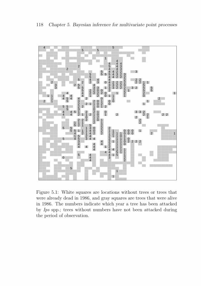
118 Chapter 5. Bayesian inference for multivariate point processes
4 55 5
14
4 4 42 5 4 3
2 4 4 35 4 4 2 2 3
5 5 5 5 4 3 2 35 4 4 2 2 2
5 4 4 4 2 2 22 2 2 3 0 4 2 2 2 2 2 2 1 1
3 2 5 4 3 3 2 2 0 53 5 5 3 3 1 3 3 2 2 2 3 2 5 5
5 2 2 0 0 2 2 1 5 54 4 2 2 2 2 0 1 2 2 1
1 1 4 4 4 1 2 0 1 1 1 01 4 5 4 4 2 0 1 2
2 1 5 3 2 0 1 0 0 12 2 1 1 0 2 0 1
5 5 2 2 1 0 1 25 3 0
4 4 5 1 2 2 1 0 3 3 24 4 2 1 1 2 1 0 1 2 2 2 2 2
0 1 2 2 12 2 2 1 0 1 2
1 1 1 2 1 25 2 1 5 2
5 5 1 3 0 2 25 5 1 1 1 4 0 2 1 1 0 0 0 1
4 2 1 4 2 2 1 2 1 1 0 0 0 2 11 5 2 4 2 1 1 0 1
5 4 5 3 4 4 2 1 1 1 03 4 2 1 1 1 0 2 2 2 24 4 4 2 1 1 04 4 4 1 2 1 1
4 4 4 1 1 14 4 5 1 1
5 4 4 1 5 10 4 3 2
4 2
51
1
Figure 5.1: White squares are locations without trees or trees thatwere already dead in 1986, and gray squares are trees that were alivein 1986. The numbers indicate which year a tree has been attackedby Ips spp.; trees without numbers have not been attacked duringthe period of observation.
5.2. Notation 119
as for more general models.
5.2 Notation
The data were collected during autumn, when Ips spp. were dormantuntil the beginning of the next attack period the following spring. Forconvenience we can therefore assume that the data were observed atthe times k = 0, 1, . . . , 5 which correspond to the end of the years1987, 1988, . . . , 1992. Further, we let k = −1 correspond to the endof year 1986, and we say that time t is in year k if k − 1 < t ≤ k.
We let i = 1, . . . , 807 index the sites, i.e. the locations with livingtrees at time −1. Let yt,i = 0 if site i has not been previously attackedby Ips spp. at time t, yt,i = 1 if it has been attacked earlier in thesame year, and yt,i = 2 if it has been attacked in a previous year. Byan “event” at the tree i we mean a transition of the zero-one processvt,i = 1[yt,i ≥ 1], where 1[·] denotes the indicator function. We denotethe time of this transition ti. We do not consider a transition 1 → 2for yt,i as an event, since it is certain that this transition happens atthe end of the year at which the event took place. Note that thereis a one-to-one correspondence between the process vs,i for s < t (ors ≤ t) and the process ys,i for s < t (or s ≤ t).
The process vs = (vs,1, . . . , vs,807) is a particular kind of multivari-ate point process (or counting process), where each vt,i is restrictedto be either zero or one. Such a process is specified by the condi-tional intensity function (Daley and Vere-Jones, 2003): For each treei, given the history of the process vs for times s < t, let
λt,i = E [dvt,i| (vs)s<t] /dt
denote the conditional intensity of the tree being attacked by Ips spp.In the next section we specify models for the conditional intensity,allowing λt,i to depend on covariate information (xs,i)s<t, where xt,i
denotes the number of turpentine beetles at time t and site i. It willalso depend on external information related to Ips spp. activity and

120 Chapter 5. Bayesian inference for multivariate point processes
on “neighboring information”. For a site i, consider its first-, second-,... order neighbors, which are the (up to) four nearest, four secondnearest,... sites to i, and let Ni denote the set of first to fifth orderneighbors of i. Finally, let ut,i = 1[yt,i = 1] and let nt,i =
∑
j∈Niut,j
be the number of neighbors of i that are infested with Ips spp. bytime t in the same year.
5.3 Model
As usual, t− means the time just before time t. Assume that for t inyear k,
λt,i = 1[vt−,i = 0]ρ(t){
ψ0 + ψ1nα1
t−,i + ψ2nα2
(k−1)−,i+ ψ3xk−,i
}
(5.1)
where ρ is a non-negative function, ψ0, ψ1, ψ2, ψ3 are non-negativeparameters, and α1 = α2 = 2 (this choice and alternative models arediscussed at the end of this section). The term 1[vt−,i = 0] is included,since Ips spp. do not attack the same tree twice. The meaning of theother terms in (5.1) is given below.
The function ρ incorporates external information about Ips spp.activity due to seasonal variation. Figure 5.2 shows ρ and reflects thefact that Ips spp. has a window of activity about four-five monthsand normally peak around July. Specifically, for t in year k, ρ(t) =ϕ((t− µk)/σk) where ϕ is the standard normal density function andthe parameters µk and σk are determined as follows. Aukema et al.(2005) modeled Ips spp. activity as the number of Ips spp. caught intraps every week during the flight period in 2001–2002, using a linearregression model with various explanatory variables, but only thetemperature is available in our study. Therefore we refit the modelwith temperature as the only explanatory variable, and estimate µk
and σk by the empirical mean and standard deviation obtained frompredicting the number of Ips spp. that would have been caught duringeach week of the kth year. Since µk − k and σk do not depend
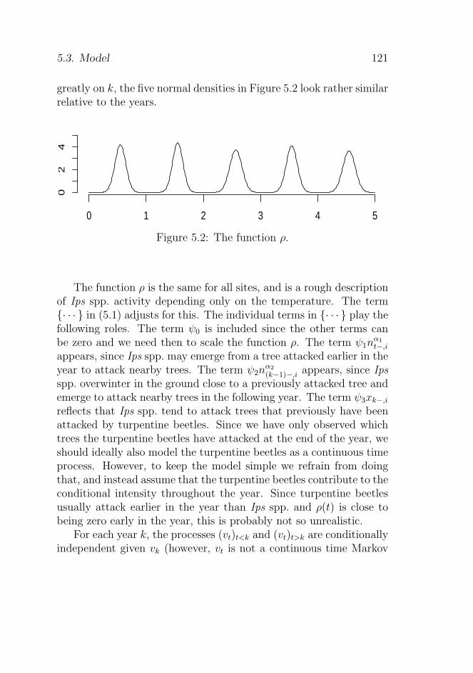
5.3. Model 121
greatly on k, the five normal densities in Figure 5.2 look rather similarrelative to the years.
0 1 2 3 4 5
02
4
Figure 5.2: The function ρ.
The function ρ is the same for all sites, and is a rough descriptionof Ips spp. activity depending only on the temperature. The term{· · · } in (5.1) adjusts for this. The individual terms in {· · · } play thefollowing roles. The term ψ0 is included since the other terms canbe zero and we need then to scale the function ρ. The term ψ1n
α1
t−,i
appears, since Ips spp. may emerge from a tree attacked earlier in theyear to attack nearby trees. The term ψ2n
α2
(k−1)−,iappears, since Ips
spp. overwinter in the ground close to a previously attacked tree andemerge to attack nearby trees in the following year. The term ψ3xk−,i
reflects that Ips spp. tend to attack trees that previously have beenattacked by turpentine beetles. Since we have only observed whichtrees the turpentine beetles have attacked at the end of the year, weshould ideally also model the turpentine beetles as a continuous timeprocess. However, to keep the model simple we refrain from doingthat, and instead assume that the turpentine beetles contribute to theconditional intensity throughout the year. Since turpentine beetlesusually attack earlier in the year than Ips spp. and ρ(t) is close tobeing zero early in the year, this is probably not so unrealistic.
For each year k, the processes (vt)t<k and (vt)t>k are conditionallyindependent given vk (however, vt is not a continuous time Markov
122 Chapter 5. Bayesian inference for multivariate point processes
process). We therefore condition on v0 and consider the likelihoodfunction based on the remaining data d = (vt)0<t≤5 (i.e. including themissing data on the time interval [0, 5]). Letting ψ = (ψ0, ψ1, ψ2, ψ3),the likelihood is
L(ψ; d|v0) =5∏
k=1
[
∏
i: k−1<ti≤k
λti,i
]
exp
(
−
∫ k
k−1
∑
i
λt,i dt
)
. (5.2)
Furthermore, we specify an improper uniform prior for ψ on [0,∞)4.Thus the conditional density of ψ given d (and v0) is proportional tothe likelihood (5.2). A rigorous proof that this conditional distri-bution of ψ is proper seems difficult, but from a practical point ofview we would expect the MCMC runs described in Section 5.4.1 todiverge if the distribution was improper. This is not the case, andalternatively we could replace the range of ψ by a very large butbounded region.
Actually, before considering the model (5.1), we analyzed themodel with
λt,i = ρ(t) exp(
ψ0 + ψ1nt−,i + ψ2n(k−1)−,i + ψ3xk−,i
)
,
where ψ0, ψ1, ψ2, ψ3 are real parameters. This model is of a somewhatsimilar form as the model in Zhu et al. (2006), but a model checkalong similar lines as in Section 5.4.2 showed that the model didnot fit the data well. Partly inspired by the form of the Hawkesprocess (Hawkes, 1971; Daley and Vere-Jones, 2003), we then turnedto the model (5.1) but with α1 = α2 = 1. We observed a misfit andconsidered therefore alternative values α1, α2 ∈ {0, 1, 2}. We finallyconcluded that the model (5.1) with α1 = α2 = 2 fit best.
5.4 Inference
5.4.1 Posterior simulation and estimation
The posterior distribution is the conditional joint distribution of ψand the missing data on [0, 5] given the observations y0, y1, . . . , y5.
5.4. Inference 123
We use a Metropolis-within-Gibbs algorithm to simulate from theposterior distribution — we assume that the reader is familiar withMarkov chain Monte Carlo (MCMC) methods; see e.g. Robert andCasella (2004).
Specifically, we propose to update each of the four parametersψ0, ψ1, ψ2, ψ3 one at a time using Metropolis random walk steps withnormal proposal distributions, where the proposal variances are cho-sen to reach an average acceptance ratio of approximately 0.25 (Ro-berts et al., 1997). Moreover, within a given year k at a site i eitherone event ti ∈ (k − 1, k] has happened, where we do not know theexact value of ti, or nothing has happened. If an event has happenedat site i, we need to simulate the unknown ti from its conditional dis-tribution given “everything else”, i.e. from the density proportionalto λt,i, with t ∈ (k − 1, k]. We do this by visiting all the sites withevents in some pre-determined order, updating ti by an independentMetropolis sampler with proposal density ρ(t), t ∈ (k − 1, k].
Figure 5.3 shows plots of the posterior distributions of ψ0, ψ1, ψ2,ψ3 based on an MCMC run length of 100,000 with a burn-in lengthof 1,000. Note that all of the parameters are clearly bounded awayfrom zero. Obviously, since ψ1 respective ψ2 is significant, the prob-ability that a tree is going to be attacked increases when more treesin the neighborhood have been attacked earlier in the year respectivein the previous year. This leads to several potential biological mech-anisms. One is that once a beetle enters a tree and emits aggregationpheromones (Wood, 1982), large numbers of beetles from previouslyattacked neighboring trees are available to respond and hence rapidlyexhaust the tree’s defenses (Raffa and Berryman, 1983). Second, fac-tors that predispose trees to being susceptible to attack may be dis-tributed in a highly clustered fashion, and the resident populationof beetles again respond to the first entries thereby generating theobserved pattern (Erbilgin and Raffa, 2003). Obviously these are notmutually exclusive. Finally, the significance of ψ3 in (5.1) impliesthat trees are more susceptible to being attacked by Ips spp. if theyhave been attacked by turpentine beetles previously.
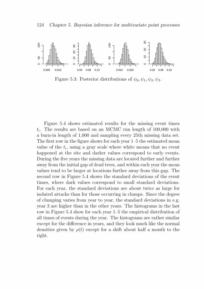
124 Chapter 5. Bayesian inference for multivariate point processes
0.005 0.015
05
01
50
0.04 0.08 0.120
10
20
30
0.010 0.020
05
01
50
0.02 0.06 0.10
01
02
03
0
Figure 5.3: Posterior distributions of ψ0, ψ1, ψ2, ψ3.
Figure 5.4 shows estimated results for the missing event timesti. The results are based on an MCMC run length of 100,000 witha burn-in length of 1,000 and sampling every 25th missing data set.The first row in the figure shows for each year 1–5 the estimated meanvalue of the ti, using a gray scale where white means that no eventhappened at the site and darker values correspond to early events.During the five years the missing data are located further and furtheraway from the initial gap of dead trees, and within each year the meanvalues tend to be larger at locations further away from this gap. Thesecond row in Figure 5.4 shows the standard deviations of the eventtimes, where dark values correspond to small standard deviations.For each year, the standard deviations are about twice as large forisolated attacks than for those occurring in clumps. Since the degreeof clumping varies from year to year, the standard deviations in e.g.year 3 are higher than in the other years. The histograms in the lastrow in Figure 5.4 show for each year 1–5 the empirical distribution ofall times of events during the year. The histograms are rather similarexcept for the difference in years, and they look much like the normaldensities given by ρ(t) except for a shift about half a month to theright.

5.4. Inference 125
0.0 0.2 0.4 0.6 0.8 1.0
01
23
4
1.0 1.2 1.4 1.6 1.8 2.0
01
23
4
2.0 2.2 2.4 2.6 2.8 3.0
01
23
4
3.0 3.2 3.4 3.6 3.8 4.0
01
23
4
4.0 4.2 4.4 4.6 4.8 5.0
01
23
4
Figure 5.4: Columns: years 1, 2, 3, 4, 5. First row: gray scale plotsof estimated mean event times. Second row: gray scale plots of esti-mated standard deviations of event times. Last row: histograms ofall event times and ρ(t) within each year.

126 Chapter 5. Bayesian inference for multivariate point processes
5.4.2 Model checking
Following the idea of posterior predictive model checking (Gelmanet al., 1996), we consider posterior predictions: for each l = 1, 2, . . .,we simulate a realization from the posterior distribution and use thiswhen simulating “new data” u
(l)t,i and v
(l)t,i from the observation model;
see Appendix A. For convenience, let u(0)t,i = ut,i and v
(0)t,i = vt,i denote
the data.
To check how well the model fits the data, we first consider thenumber of attacks in each year,
w(l)1 (t) =
∑
i
u(l)t,i ,
where t = 1, . . . , 5. The left plot in Figure 5.5 shows the 2.5, 50, 97.5percentiles estimated from w
(l)1 (t) for l = 0, . . . , 199. The values of
w(0)1 (t) is also shown in the figure. In all years except year 3 where
the number of Ips spp. attacks was particularly low, w(0)1 (t) is located
in the central interval.
Second, let d(i, j) denote Euclidean distance between site i andj. For δ ≥ 1,
w(l)2 (δ) =
∑
i<j: d(i,j)∈(δ−1,δ]
v(l)5,iv
(l)5,j,
is the number of pairs of sites between δ−1 and δ apart and attackedat some time during the observation period. Thus w
(l)2 (δ) quantifies
the degree of spatial clustering. The center plot in Figure 5.5 showsw
(l)2 (δ) for δ = 1, . . . , 5 in the same way as in the first plot. Again
there are no discrepancies between the model and the data.
Third, in order to combine temporal and spatial information, con-sider the number of neighboring sites that are attacked in years timet apart,
w(l)3 (t) =
∑
i,j,k: j∈Ni,k=t,...,5
u(l)k,iu
(l)k−t,j
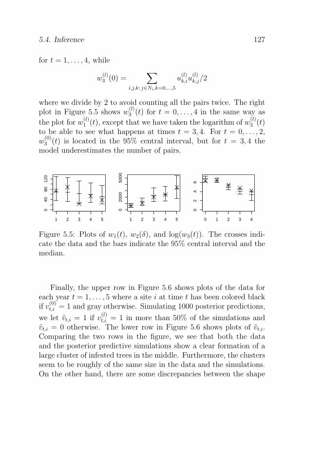
5.4. Inference 127
for t = 1, . . . , 4, while
w(l)3 (0) =
∑
i,j,k: j∈Ni,k=0,...,5
u(l)k,iu
(l)k,j/2
where we divide by 2 to avoid counting all the pairs twice. The rightplot in Figure 5.5 shows w
(l)3 (t) for t = 0, . . . , 4 in the same way as
the plot for w(l)1 (t), except that we have taken the logarithm of w
(l)3 (t)
to be able to see what happens at times t = 3, 4. For t = 0, . . . , 2,w
(0)3 (t) is located in the 95% central interval, but for t = 3, 4 the
model underestimates the number of pairs.
1 2 3 4 5
04
08
01
20
1 2 3 4 5
02
00
05
00
0
0 1 2 3 4
02
46
Figure 5.5: Plots of w1(t), w2(δ), and log(w3(t)). The crosses indi-cate the data and the bars indicate the 95% central interval and themedian.
Finally, the upper row in Figure 5.6 shows plots of the data foreach year t = 1, . . . , 5 where a site i at time t has been colored blackif v
(0)t,i = 1 and gray otherwise. Simulating 1000 posterior predictions,
we let vt,i = 1 if v(l)t,i = 1 in more than 50% of the simulations and
vt,i = 0 otherwise. The lower row in Figure 5.6 shows plots of vt,i.Comparing the two rows in the figure, we see that both the dataand the posterior predictive simulations show a clear formation of alarge cluster of infested trees in the middle. Furthermore, the clustersseem to be roughly of the same size in the data and the simulations.On the other hand, there are some discrepancies between the shape
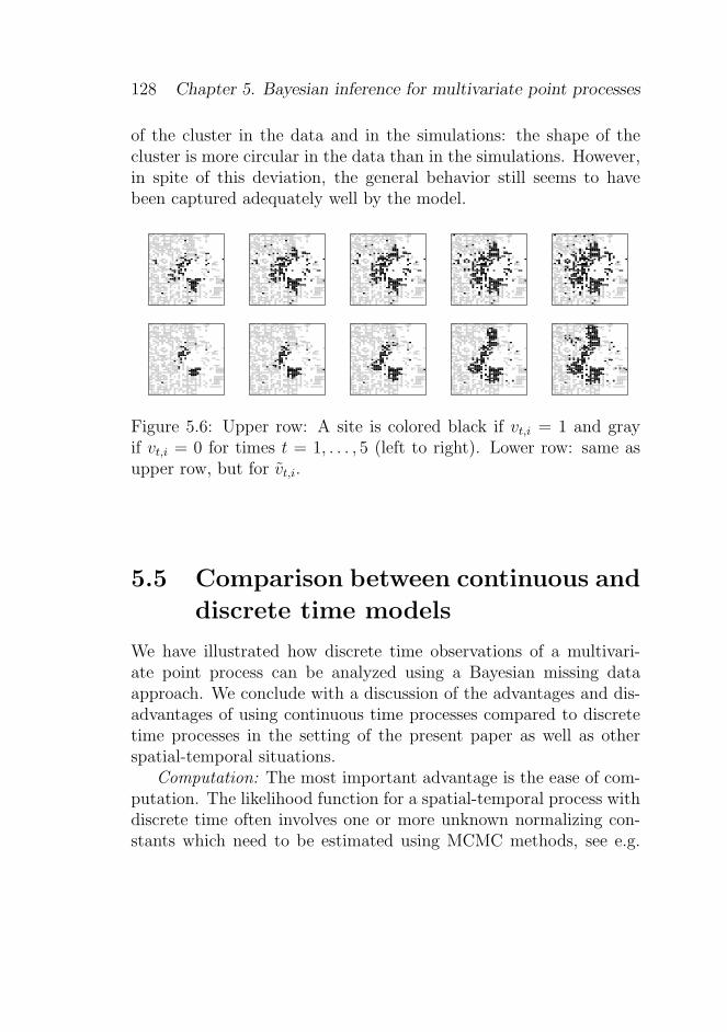
128 Chapter 5. Bayesian inference for multivariate point processes
of the cluster in the data and in the simulations: the shape of thecluster is more circular in the data than in the simulations. However,in spite of this deviation, the general behavior still seems to havebeen captured adequately well by the model.
Figure 5.6: Upper row: A site is colored black if vt,i = 1 and grayif vt,i = 0 for times t = 1, . . . , 5 (left to right). Lower row: same asupper row, but for vt,i.
5.5 Comparison between continuous and
discrete time models
We have illustrated how discrete time observations of a multivari-ate point process can be analyzed using a Bayesian missing dataapproach. We conclude with a discussion of the advantages and dis-advantages of using continuous time processes compared to discretetime processes in the setting of the present paper as well as otherspatial-temporal situations.
Computation: The most important advantage is the ease of com-putation. The likelihood function for a spatial-temporal process withdiscrete time often involves one or more unknown normalizing con-stants which need to be estimated using MCMC methods, see e.g.
5.5. Comparison between continuous and discrete time models 129
the Markov random field models in Besag and Tantrum (2003) andZhu et al. (2006). In contrast the likelihood function for a multivari-ate point process is completely specified by modeling the conditionalintensity, cf. equation (5.2). In Zhu et al. (2006), we modeled thedata set consisting of the three types of data given by turpentinebeetles, Ips spp. and tree conditions. The likelihood function for thismodel factorized into three terms, one for each type of data, wherewe can compare the term corresponding to Ips spp. and the modelused in the present paper, when we include the Ips spp. at all sites(rather than restricting the data to the subset of sites considered sofar in the present paper). For this particular comparison, the com-putation time of the MCMC algorithm for posterior distributions forthe discrete time model is roughly two hundred times longer thanthe corresponding computation time for the continuous time model.This improvement in speed means that we have been able to investi-gate several variations of the model (5.1) (see the end of Section 5.3),something we could not do within practical time limits in the caseof the discrete time process for Ips spp. in Zhu et al. (2006). On theother hand, in Zhu et al. (2006) the likelihood terms correspondingturpentine beetle colonization and tree conditions were easy to spec-ify, and calculations for these terms were very fast. Extending thecontinuous time model to include turpentine beetles and tree condi-tions may be much more involved, and a comparison between sucha model and the full model in Zhu et al. (2006) may well turn outdifferently.
External information: For a discrete time process as compared toa continuous time process, it may be difficult to incorporate external(or, in a broad sense, covariate) information in the form of anotherstochastic process observed at a different time scale than the discretetime process. For example, the ρ term in (5.1) incorporates externalinformation about Ips spp. activity due to seasonal variation; suchinformation can only be incorporated into the model in Zhu et al.(2006) after some form of aggregation. On the other hand, we re-quire the external information that was collected in the field across
130 Chapter 5. Bayesian inference for multivariate point processes
a full season of Ips spp. activity modeled into ρ to obtain a realis-tic continuous time model for Ips spp. attacks. If we had no suchinformation or only unreliable information available, the continuoustime model approach would be problematic. It would also be a prob-lem if the modeling form of ρ is misspecified. Specifying ρ is timeconsuming, and this partially offsets the advantage of the shortercomputation time for the continuous time model.
Time scale comparability: While the parameters of two continuoustime processes may be compared even if their time scales for obser-vations (i.e. time lengths between observation times) are different, itmay not be meaningful to compare the parameters of two discretetime processes with different time scales. The choice of observationtimes in Zhu et al. (2006) is biologically meaningful, since we haveannual observation after cessation of insect activity; however, sup-pose that we had another data set with observations every secondyear. Further, imagine that we wish to use a model of the same formas in Zhu et al. (2006) for this other data set. Then, because ofthe different time scales, we cannot directly compare the parametersgoverning e.g. Ips spp. activity.
Consistency: Although observed only at discrete times, the typesof data considered in the present paper come from an underlyingcontinuous time process, and the existence of an underlying continu-ous time process is not ensured by specifying a discrete time process.Obviously, this is not an issue when we have specified a continuoustime model, but our continuous time model only approximates thecomplexity of the system under study. Indeed, Ips spp. colonizationdoes not occur exactly at one time point; it is a complicated processinvolving hundreds or thousands of beetles attacking over a short pe-riod of time. On the other hand, the discrete time model reflects thecumulative Ips spp. attacks throughout the past season, and in thissense it is a perfectly sensible model for the system under study.
Estimation of missing data: A continuous time process allows usto model what has happened between observation times, where in ourcase the event times of within-season Ips spp. attacks can be readily
5.5. Comparison between continuous and discrete time models 131
estimated by the MCMC algorithm in Section 5.4.1. In contrast it isnot possible to do this kind of estimation for missing data based onthe model in Zhu et al. (2006), although it was not a part of the sci-entific objectives there. In the present paper, the estimates providesome trustful qualitative results regarding how the times of eventsdepend on the distance to the gap of dead trees and the similar be-havior over the years. However, quantitative results depend much ona careful modeling of external information, particularly the functionρ.
Predictions: It is straightforward to predict what may happen atany time after the final observation time, applying Ogata’s modifiedthinning algorithm for the continuous time process in the presentpaper (see Appendix A). The discrete time model in Zhu et al. (2006)allows us only to predict what may happen annually.
In conclusion, spatial-temporal processes often suffer from beingcomputationally intensive, and we have demonstrated that in thepresent case, using a continuous time process is indeed a viable al-ternative to a discrete time process.
Appendix A
For model checking in Section 5.4.2, we need to simulate new datafrom the observation model. For this we use Ogata’s modified thin-ning algorithm extended to marked processes (Daley and Vere-Jones,2003; Ogata, 1981).
Factorize the intensity, λt,i = λt × p(i|t), where λt =∑
i λt,i is theintensity for the temporal process of events disregarding the location,and p(i|t) ∝ λt,i is the probability function for the location giventhe time of the event. Note that the dependence on the past events(locations and times) of both functions are suppressed in the notation.Furthermore, define two functions l(t) and m(t) by l(t) = t+ 0.1 fork−1 < t ≤ µk and l(t) = k for µk < t ≤ k, and m(t) = maxs∈[t,l(t)] λs.Ogata’s modified thinning algorithm is then started at time t = 0 and
132 Chapter 5. Bayesian inference for multivariate point processes
the following steps are repeated until t > 5:
1. Compute l(t) and m(t).
2. Generate an exponentially distributed variable T with inversemean m(t) and a uniform variable U on [0, 1] independently ofeach other.
3. If T > l(t), set t = t+ l(t).
4. Else if t+ T > 5 or U > λt+T/m(t), set t = t+ T .
5. Otherwise, let the next event be ti = t+T , where i is generatedusing the probability function p(i|t), and set t = t+ T .
The output is the set of all ti obtained in step 5.Combining this algorithm with a sample of the posterior distri-
butions in Section 5.4.1, we get posterior predictions. In practice weget a sample of the posterior distributions by taking values from theMarkov chains at regular intervals chosen such that the sample iseffectively independent.
Acknowledgments
This work was supported by the Danish Natural Science ResearchCouncil, USDA NRI (2003-3502-13528), NSF (DEB0314215), andthe UW-Madison College of Agricultural and Life Sciences. We aregrateful to the Wisconsin Department of Natural Resources for pro-viding the study site.
References
Aukema, B. H., Clayton, M. K., and Raffa, K. F. (2005). Modelingflight activity and population dynamics of the pine engraver, Ipspini, in the Great Lakes region: Effects of weather and predatorsat short time scales. Population Ecology , 47, 61–69.
5.5. Comparison between continuous and discrete time models 133
Besag, J. and Tantrum, J. (2003). Likelihood analysis of binary datain space and time. In P. J. Green, N. L. Hjort, and S. Richard-son, editors, Highly Structured Stochastic Systems, pages 289–295.Oxford University Press, Oxford.
Daley, D. J. and Vere-Jones, D. (2003). An Introduction to the Theoryof Point Processes, Volume I: Elementary Theory and Methods .Springer, New York, 2nd edition.
Erbilgin, N. and Raffa, K. F. (2003). Spatial analysis of forest gapsresulting from bark beetle colonization of red pines experiencingbelowground herbivory and infection. For. Ecol. & Manag., 177,145–153.
Furniss, R. L. and Carolin, V. M. (1980). Western Forest Insects .USDA FS Misc. Publ. 1339. Washington DC. 654 pp.
Gelman, A., Meng, X. L., and Stern, H. S. (1996). Posterior pre-dictive assessment of model fitness via realized discrepancies (withdiscussion). Statistica Sinica, 6, 733–807.
Hawkes, A. G. (1971). Spectra of some self-exciting and mutuallyexciting point processes. Biometrika, 58, 83–90.
Ogata, Y. (1981). On Lewis’ simulation method for point processes.IEEE Transactions on Information Theory , IT-27, 23–31.
Raffa, K. F. and Berryman, A. A. (1983). The role of host plantresistance in the colonization behavior and ecology of bark beetles.Ecol. Monogr., 53, 27–49.
Robert, C. and Casella, G. (2004). Monte Carlo Statistical Methods .Springer, New York, 2nd edition.
Roberts, G. O., Gelman, A., and Gilks, W. R. (1997). Weak conver-gence and optimal scaling of random walk Metropolis algorithms.Annals of Applied Probability , 7, 110–120.
134 Chapter 5. Bayesian inference for multivariate point processes
Wood, D. L. (1982). The role of pheromones, kairomones, and al-lomones in the host selection and colonization behavoir of barkbeetles. Ann. Rev. of Entomol., 27, 411–446.
Zhu, J., Rasmussen, J. G., Møller, J., Aukema, B. H., and Raffa, K.(2006). Spatial-temporal modeling of forest gaps generated by col-onization from below- and above-ground beetle species. Researchreport R-2006-04, Department of Mathematical Sciences, AalborgUniversity. Available at http://www.math.aau.dk/∼jm. (Submit-ted for publication).

Chapter 6
Software and work in
progress
6.1 Software
Since all the papers included in this thesis have been computation-ally heavy and required much programming, I have added this sec-tion describing some (though far from all) of the many programsused. This allows other people to use or be inspired by the programs.Section 6.1.1 describes some general issues of the programs, and Sec-tions 6.1.2–6.1.4 are dedicated to the specific programs used in eachchapter. I assume that the reader is familiar with the correspondingtheoretical chapters before reading the following sections.
6.1.1 Downloading, compiling and running pro-
grams
All the implementations have been done in C++ on a Linux system,but should work equally well on Windows. The files needed can bedownloaded from
www.math.aau.dk/∼jgr/downloads/
135
136 Chapter 6. Software and work in progress
where the name of the file needed is stated in each of the followingsections. All files have been compressed using zip, and can be uncom-pressed using the command unzip filename (on a Linux system).The specific files retrieved from the compressed file are described inthe following sections. To compile one of the programs on a Linuxsystem, use the command
g++ -o outputfile inputfile -lm
where inputfile is the name of the C++ source code file to be com-piled, and outputfile is the user-specified name of the programfile to be generated. The program is then run with the commandoutputfile. Any parameters should be set in inputfile prior tocompiling and running the program; the parameters are describedin the following sections. Note that only the files described as mainprograms in the following sections can be compiled and run; tryingto compile other files will result in an error.
6.1.2 Software for Chapters 2 and 3
This section explains the use of some of the programs I have used forsimulating Hawkes processes in Chapters 2 and 3. From Chapter 2, Ihave included the perfect simulation algorithms (Algorithms 2.2 and2.3 combined) for the Hawkes process with exponentially decaying off-spring intensity (Example 2.1) and the birth and death type Hawkesprocess with exponential life times (Example 2.2). From Chapter 3, Ihave included the approximate simulation algorithm (Algorithm 3.1)for the same examples.
All the files needed can be extracted from the file SimHawkes.zipas described in Section 6.1.1. There are two types of files included.The first type are the main programs for simulating the two processeswith the two algorithms:
• SimHawkesASExp.cpp: Approximate simulation of the Hawkesprocess with exponential offspring intensity.

6.1. Software 137
• SimHawkesASBD.cpp: Approximate simulation of the birth-deathHawkes process.
• SimHawkesPSExp.cpp: Perfect simulation of the Hawkes pro-cess with exponential offspring intensity.
• SimHawkesPSBD.cpp: Perfect simulation of the birth-death Haw-kes process.
The other files contain the algorithms that the main programs use(these files cannot be compiled and run as separate programs). Thefiles are:
• SimHawkesTools.cpp: Basic tools needed by the other pro-grams.
• SimHawkesExp.cpp: Simulation algorithms for the Hawkes pro-cess with exponential offspring intensity.
• SimHawkesBD.cpp: Simulation algorithms for the birth-deathHawkes process with exponential life times.
Prior to compiling and running the programs, various parametersfound in the main programs can be changed:
• mu > 0: The intensity of the immigrant process.
• 0 < alpha < 1: The mean number of offspring generated byany event.
• beta > 0: The parameter used in the exponential offspringintensity (for the Hawkes process with exponential offspringintensity) or the inverse mean of life times (for the birth-deathHawkes process).
• tplus > 0: Simulation interval is [0, tplus].

138 Chapter 6. Software and work in progress
• tminus ≤ 0: Starting value for approximate simulation algo-rithms, i.e. the approximate simulation algorithm simulates im-migrants on the interval [tminus, tplus]
• ngrid ∈ N: Number of grid points used in quadrature rule forapproximating integrals in perfect simulation algorithms. Notethat this should not be set too low.
See Chapters 2 and 3 for more details on the parameters.The output of either one of the four main programs is a text-file
called either hawkesexp.dat or hawkesbd.dat depending on whetherit is a Hawkes process with exponential offspring intensity or a birth-death Hawkes process. The file hawkesexp.dat contains one col-umn of simulated event times. The file hawkesbd.dat contains twocolumns of real numbers - the first one is the event times, and thesecond one is the marks (i.e. life times).
6.1.3 Software for Chapter 4
This section describes the implementation of one of the algorithmsused in Chapter 4. This is the MCMC algorithm for approximat-ing the posterior distribution of parameters (ψ0, ψ1, ψ2, ψ3) (see Sec-tion 4.4 for details). The reason for only including this single programout of the many programs used is that it contains most of the inter-esting algorithms (e.g. perfect simulation and path sampling), andalready it is rather comprehensive.
The files included can be extracted from BeetlesTrees.zip asdescribed in Section 6.1.1. The following file contain the main pro-gram:
• mcmc psi path.cpp: The main program for the MCMC runsfor approximating the posterior distributions of the parame-ters (ψ0, ψ1, ψ2, ψ3) using path sampling for approximating theunknown normalizing constants.
The algorithms used by the main programs are included in the fol-lowing files (these files cannot be compiled and run):

6.1. Software 139
• data.cpp: Algorithms for loading data and creating neighbour-hood structures.
• sim autolog process.cpp: Algorithms for making perfect sim-ulations of autologistic processes.
• random.c and random.h: Algorithms for simulating randomvariables.
Finally all files with the extension .dat are data files. Note that sincethe data is not publicly available the files included are fake data, i.e.the data is fine for illustrative purposes, but will not give the sameresults as those obtained in Chapter 4.
• turp87sim.dat,. . . ,turp92sim.dat: Matrices of turpentine bee-tle data for each year, where each entry indicates the state ofthe tree at a position in a regular grid; an entry of -1 meansthere is no tree at the position, 0 means that the tree at thisposition has not been attacked at this time, an entry largerthan 0 means that this number of turpentine beetles is presentin the tree at this position.
• ips87sim.dat,. . . ,ips92sim.dat: Ips spp. colonization datarepresented as a matrix for each year; an entry of -1 meansthere is no tree at the position, 0 means that the tree has notbeen attacked at this time, 1 means it has been attacked.
• trees86sim.dat,. . . ,trees92sim.dat: Matrices of tree condi-tion data for each year; an entry of -1 means there is no treeat the position, 0 means that the tree at this position is alive,and 1 means that it is dead.
The program contains the following parameters that can be ad-justed before compiling and running the programs:
• NumSteps: Number of steps used in the MCMC run. Note thatthe algorithm is rather slow, and setting NumSteps too highmay result in a very long running time.

140 Chapter 6. Software and work in progress
• NumSim: Number of perfect simulations used in the approxima-tion of the normalizing constants when using path sampling.
• sigma0,. . . ,sigma3: Standard deviations used in the normallydistributed proposals for each of the four parameters.
The output of the program is a file named mcmc psi.dat con-taining a matrix with one row for each step in the MCMC run.Each row has five columns: the first four entries are the values of(ψ0, ψ1, ψ2, ψ3) and the last row contains the acceptance ratio for thisparticular MCMC step. This output is also written to the screenwhen the program is running.
6.1.4 Software for Chapter 5
This section describes some of the programs used in Chapter 5.Specifically, the software described is the implementations of theMCMC algorithms for approximating the posterior distribution of pa-rameters (see Section 5.4.1) and Ogata’s modified thinning algorithmfor generating posterior predictions (see Appendix A in Chapter 5).
The files needed can be extracted from the file BeetlesCont.zip
as described in Section 6.1.1. The following files contain the mainprograms:
• mcmcclin.cpp: MCMC algorithms for approximating posteriordistributions of the parameters in the model.
• csimclin.cpp: Algorithms for simulating event times, i.e. thetimes of Ips spp. attacks.
The algorithms used by the main programs are included in the fol-lowing files (these files cannot be compiled and run):
• datac.cpp: Algorithms for loading data and creating neigh-bourhood structures.
6.1. Software 141
• thinningclin.cpp: Ogata’s modified thinning algorithm usedfor simulating times of Ips spp. attacks.
• random2.c and random2.h: Algorithms for simulating randomvariables.
Finally all files with the extension .dat are data files. As in Sec-tion 6.1.3, the data is not the real data, and will not give the sameresults as those obtained in Chapter 5.
• rho.dat: Coefficients for ρ(t).
• ips87sim.dat,. . . ,ips92sim.dat: Ips spp. data represented asa matrix; an entry of -1 means there is no tree at the position,0 means that the tree has not been attacked at this time, 1means it has been attacked.
• turp87sim.dat,. . . ,turp92sim.dat: Turpentine beetles datarepresented as a matrix; an entry of -1 means there is no treeat the position, 0 means that the tree has not been attackedat this time, an entry larger than 0 means that this number ofturpentine beetles is present in the tree.
• treessim.dat: Tree data represented as a matrix; an entry of-1 means there is no tree at the position, 0 means that the treeis alive, 1 means it is dead. Only positions with living trees areused by the algorithm.
The program mcmcclin.cpp contains the following parametersthat can be adjusted before compiling and running the programs:
• NumSteps: Number of steps used in the MCMC algorithm.
• inc0,. . . ,inc6: Various models have been tried in Chapter 5,and the programs described in this section not only includes thefour parameters (ψ0, ψ1, ψ2, ψ3) from model (5.1) in Chapter 5,but also three other parameters. In the program the parameters
142 Chapter 6. Software and work in progress
are numbered 0, . . . , 6, and the parameters numbered (0, 2, 4, 5)correspond to (ψ0, ψ1, ψ2, ψ3). Parameters (1, 3) corresponds to(ψ1, ψ2) but without squaring, and parameter 6 corresponds toψ3 but with xk−,i squared. Setting incx equal to one, wherex = 0, . . . , 6, includes the corresponding term.
• sd0,. . . ,sd6: Standard deviations used for making normally dis-tributed proposals in the MCMC algorithm for each of the sevenparameters.
The output of the program mcmcclin.cpp is a file called psi.dat con-taining a matrix, which includes a row for each step in the MCMCrun. Each row contains 14 entries of parameter values and accep-tance ratios; the first two entries contain the parameter value andacceptance ratio for parameter 0, entries three and four contain theparameter value and acceptance ratio for parameter 1, and so on.Any parameter not included (i.e. by setting incx equal to zero, wherex = 0, . . . , 6) is set equal to zero in this file.
The program csimclin.cpp contains the following parameters:
• type: If type equals 0 the parameters used in the simulation istaken from the file psi.dat (i.e. it can be considered a randomdraw from the posterior distributions of the parameters), andif it equals 1 the parameters are user-specified.
• step: In the case of parameters being taken from psi.dat,this specifies which step in the Markov chain the parametersare taken from.
• psi0,. . . ,psi6: In the case of parameters being user-specified,these specifies the values of the seven parameters. Here the fourparameters (psi0,psi2,psi4,psi5) correspond to (ψ0,ψ1,ψ2,ψ3)from Chapter 5 as described above.
The output of this program is a matrix of times of Ips spp. attackssaved in the file simtimes.dat. An entry of -1 specifies a position
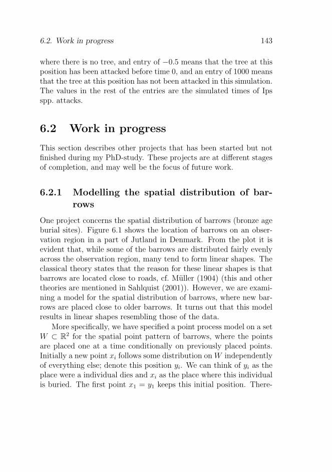
6.2. Work in progress 143
where there is no tree, and entry of −0.5 means that the tree at thisposition has been attacked before time 0, and an entry of 1000 meansthat the tree at this position has not been attacked in this simulation.The values in the rest of the entries are the simulated times of Ipsspp. attacks.
6.2 Work in progress
This section describes other projects that has been started but notfinished during my PhD-study. These projects are at different stagesof completion, and may well be the focus of future work.
6.2.1 Modelling the spatial distribution of bar-
rows
One project concerns the spatial distribution of barrows (bronze ageburial sites). Figure 6.1 shows the location of barrows on an obser-vation region in a part of Jutland in Denmark. From the plot it isevident that, while some of the barrows are distributed fairly evenlyacross the observation region, many tend to form linear shapes. Theclassical theory states that the reason for these linear shapes is thatbarrows are located close to roads, cf. Muller (1904) (this and othertheories are mentioned in Sahlquist (2001)). However, we are exami-ning a model for the spatial distribution of barrows, where new bar-rows are placed close to older barrows. It turns out that this modelresults in linear shapes resembling those of the data.
More specifically, we have specified a point process model on a setW ⊂ R
2 for the spatial point pattern of barrows, where the pointsare placed one at a time conditionally on previously placed points.Initially a new point xi follows some distribution on W independentlyof everything else; denote this position yi. We can think of yi as theplace were a individual dies and xi as the place where this individualis buried. The first point x1 = y1 keeps this initial position. There-
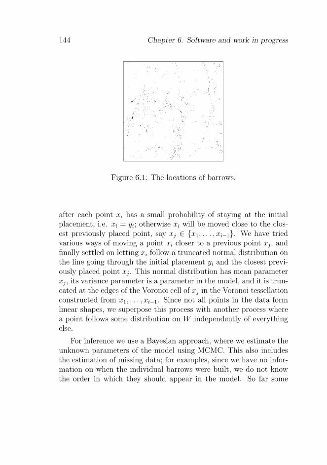
144 Chapter 6. Software and work in progress
Figure 6.1: The locations of barrows.
after each point xi has a small probability of staying at the initialplacement, i.e. xi = yi; otherwise xi will be moved close to the clos-est previously placed point, say xj ∈ {x1, . . . , xi−1}. We have triedvarious ways of moving a point xi closer to a previous point xj, andfinally settled on letting xi follow a truncated normal distribution onthe line going through the initial placement yi and the closest previ-ously placed point xj. This normal distribution has mean parameterxj, its variance parameter is a parameter in the model, and it is trun-cated at the edges of the Voronoi cell of xj in the Voronoi tessellationconstructed from x1, . . . , xi−1. Since not all points in the data formlinear shapes, we superpose this process with another process wherea point follows some distribution on W independently of everythingelse.
For inference we use a Bayesian approach, where we estimate theunknown parameters of the model using MCMC. This also includesthe estimation of missing data; for examples, since we have no infor-mation on when the individual barrows were built, we do not knowthe order in which they should appear in the model. So far some
6.2. Work in progress 145
preliminary results have been obtained using simulation, includingposterior distributions of the parameters of the model and modelchecking based on various summary statistics. These results havebeen obtained from programs I have made (except for the programsgenerating the Voronoi tessellations which have kindly been lent tous by Øivind Skare). They indicate that the model fits the data fairlywell.
We have also considered including various covariates regarding thelandscape to make a more realistic model. For example, the densityof settlements is lower in very marshy terrains than on good soil,and it seems unlikely that people would cross a big river to bury aperson on the other side. Therefore, extending the model to includeinformation about population densities on different soil types andthe difficulty of moving on certain terrain types would be useful toobtain a more realistic model. However, since the model withoutthese extensions already involves many calculations (mainly becauseof the Voronoi tessellations), the computations are already somewhatslow. It seems difficult to incorporate the landscape in a way thatis both realistic and computationally feasible. Fortunately, the datashown in Figure 6.1 seems to be quite homogeneous with respect tothe landscape, and it should be possible to obtain a realistic modelfor this particular data set without considering these covariates.
6.2.2 Biological conclusions derived from beetle
colonization models
The papers in Chapters 4 and 5 are treating the same data set fromtwo different points of view. Chapter 4 is an applied statistical pa-per where the aim is a Bayesian spatio-temporal autoregressive typeof model describing the locations of beetle attacks and tree deaths.In Chapter 5 the aim is an alternative statistical methodology, amultivariate point process model with missing data, for modeling asubset of this data. A third paper by the same authors is presentlyin preparation. This paper treats the biological implications of the
146 Chapter 6. Software and work in progress
conclusions in the two previous papers (mainly the paper treated inChapter 4). Furthermore, the paper includes an additional type ofbeetle known as root weevils (Coleoptera: Scolytidae; alt. Curculion-idae: Scolytinae).
There are two primary biological issues treated in this paper. Thefirst one is the impact of the different types of beetles on tree mortal-ity. The question here is what the role of the various types of beetlesare. For example, in Chapter 4 we discovered that Ips spp. are a causeof death of the trees, and, although turpentine beetles are not killingthe trees directly, they predipose the trees to later attacks by Ips spp.The second issue is the spatio-temporal spread of the different kindsof beetles, and how they relate to gap formations. The full biologicalimplications of the conclusions derived regarding both of these issuesare important for formulating forest management strategies.
6.2.3 Spatial Hawkes processes and applications
The Hawkes process consider in Chapters 2 and 3 can easily be gener-alized to a spatial version on R
d, see e.g. Møller and Torrisi (2005) forthe definition. As Møller and Torrisi (2005) points out, this processis a natural process for modelling the spatial spread of epidemics orindividuals from a reproducing population.
Recently the spatial Hawkes process has received some attentionfrom a theoretical point of view. Møller and Torrisi (2005) obtain ex-pressions for various summary statistics, while Bremaud et al. (2005)consider power spectra. However, there seems to be no practical workdone using the spatial Hawkes processes so far. Jesper Møller and Ihave discussed various possible data sets. Particularly, we have con-sidered the weed data set modelled in Brix and Møller (2001) andBrix and Chadoeuf (2002).
6.2. Work in progress 147
References
Bremaud, P., Massoulie, L., and Ridolfi, A. (2005). Power spectraof random spike fields and related processes. Advances in AppliedProbability , 37(4), 1116–1146.
Brix, A. and Chadoeuf, J. (2002). Spatio-temporal modeling of weedsand shot-noise G Cox processes. Biometrical Journal , 44(1), 83–99.
Brix, A. and Møller, J. (2001). Space-time multitype log gaussianprocesses with a view to modelling weed data. Scandinavian Jour-nal of Statistics , 28, 471–488.
Møller, J. and Torrisi, G. L. (2005). Second order analysis for spa-tial hawkes processes. Research Report R-2005-20, Department ofMathematical Sciences, Aalborg University.
Muller, S. (1904). Vei og bygd i sten- og bronzealderen. Aarbøger forNordisk Oldkyndighed og Historie, pages 1–64.
Sahlquist, L. (2001). Territorial behaviour and communication in aritual landscape. Geografiska Annaler , 83 B(2), 79–102.