Effects of transient climate change on basin hydrology. 1 ...

HYDROLOGICAL PROCESSESHydrol. Process. 16, 1151–1175 (2002)Published online in Wiley InterScience (www.interscience.wiley.com). DOI: 10.1002/hyp.1055

Effects of transient climate change on basin hydrology.1. Precipitation scenarios for the Arno River, central Italy

Paolo Burlando1* and Renzo Rosso2

1 Institute of Hydromechanics and Water Resources Management, ETH Zurich, ETH Honggerberg, CH-8093 Zurich, Switzerland2 Department of Hydraulic, Environmental and Surveying Engineering, Politecnico di Milano, Leonardo da Vinci 32, I-20133 Milan, Italy

Abstract:

Long-term simulations of temporal rainfall and temperature under transient global climate conditions are discussed togive an insight into potential modifications of atmospheric inputs at the basin scale in the Arno River in central Italy.The outputs from a global circulation model (GCM), simulating climate changes due to an increase in the greenhouseeffect resulting from a continuous trend in the growth of CO2 atmospheric concentration and accounting for theinfluence of both CO2 and sulphate aerosols, are downscaled using a stochastic approach based on the observed non-stationarity of precipitation and temperature patterns. By using the historical joint variability of the internal structureof storm events, one can infer future changes in storm duration and depth from GCM trend variables, thus indicatingthe extent of changes in the occurrence of wet and dry periods and in the daily rates, including those of distributionalproperties at the monthly and annual scales. Because the changes detected mainly affect the tails of the distributions,one can conclude that modifications can occur in both low and high values of rainfall at the monthly and annual scales,with a shift of the storm patterns towards shorter and more intense convective rainfall, especially in the summer season.Stochastic simulation also shows that the distributional and scaling properties of rainfall extremes may progressivelychange, thus indicating that some revision of current practices to estimate extreme storms is needed to account forpossible effects of non-stationary climate conditions. This approach provides local precipitation that, together withtemperature scenarios, can be used for hydrological simulation of basin water fluxes in the Arno River, as reported ina companion paper (Burlando P, Rosso R. Hydrological Processes this issue). Copyright 2002 John Wiley & Sons,Ltd.

KEY WORDS precipitation scenarios; climate change; stochastic downscaling

INTRODUCTION

It is widely recognized that the natural and anthropogenic production of greenhouse gases might inducemany changes in the natural environment. The most investigated of these changes are those relevantto climate—specifically to the potential increase of global and local temperatures—and to the resultingmodification of rainfall space–time distribution. These primary effects could generate a number of directand indirect impacts on the environment and the society, such as changes in water resources, increaseddesertification, loss of biodiversity, sea-level rise, and changes in agricultural productivity, as summarized forinstance, by the Special Reports of the Intergovernmental Panel on Climate Change (IPCC, 1995a–c, 1997).

During the 1980s a major focus was on global and large-scale effects of anthropogenic climate change(e.g. Manabe and Stouffer, 1980; Manabe and Wetherald, 1987), whereas attention given to regional andlocal impacts was only emphasized in the 1990s. In this respect, the study performed by Nemec and Schaake(1982) was pioneering work, in which the effect of changes in temperature and precipitation on river flowsand reservoir operation in several test catchments in North America were simulated. Since then, there hasbeen an increasing degree of research interest in both global and local effects of a potential climate change

* Correspondence to: Professor P. Burlando, Institute of Hydromechanics and Water Resources Management, ETH Zurich, ETH Honggerberg,CH-8093, Zurich, Switzerland. E-mail: [email protected]

Received 19 September 2001Copyright 2002 John Wiley & Sons, Ltd. Accepted 15 October 2001

1152 P. BURLANDO AND R. ROSSO

(e.g. Cohen, 1986; Askew, 1987; Gleick, 1987; Manabe and Wetherald, 1987; Mimikou and Kouvopoulos,1991; Burlando et al., 1997, Dvorak et al., 1997; Strzepek and Yates,1997). One should notice, however, thatgreat attention has been directed towards understanding the impact of changes of the mean climate, whereasonly a limited number of contributions assessing the variability of changes, including extreme value analysis,can be found in the literature (e.g. Burlando and Rosso, 1991; Boorman and Sefton, 1997; Mearns et al.,1997).

One can approach climate-induced non-stationarity in hydrological processes using different methods,including the analysis of palaeo-climate analogues, and that of proxy and historical data. An alternative routeis the development of hydrological simulations at the basin scale using meteorological data inputs retrievedfrom global climate scenarios, which are provided by global circulation models (GCMs). Unfortunately,the structure of GCMs is such that their space resolution is too coarse and not adequate to describe thevariability at the basin scale. Moreover, most of the models use rough representations to describe hydrologicprocesses, despite the large effort that has been made in recent years to improve the GCM components of thesoil–vegetation–atmosphere interaction (e.g. Koster and Suarez, 1994; Blyth et al., 1999). For these reasonsthere is a serious restriction in the direct use of GCM-based scenarios for investigating the possible impactsof climate change.

Identifying local climate scenarios for impact analysis, therefore, implies the definition of more detailed localscenarios by ‘downscaling’ GCMs results. This can be done by approaching the problem according to severaltechniques (Giorgi and Mearns, 1991). For instance, the improvement of high-resolution climate models, theso-called regional Climate Models (ReCMs) or limited-area models (LAMs), which use boundary conditionsobtained from the global prediction to drive a nested regional climate model, may improve the quality ofthe hydrological variables generated (Giorgi et al., 1994; Mearns et al., 1995; Ohmura et al., 1996). Nestedmodels can provide useful information on day-to-day variability and can account for forcing due to increasedgreenhouse gas concentrations. However, the reliability of this approach to analyse the local variability ofthe processes is nowadays still questionable, especially with respect to the description of precipitation and itsvariability at such small scales. Models belonging to this class are still a considerable way from providinga tool for engineering and impact analysis because of several problems. Recent contributions in the relevantliterature indeed report on systematic errors similar to those of GCMs, which increase as the LAM domainis reduced (Machenhauer et al., 1996), let alone the relatively large errors in the fundamental near-surfaceclimate parameters, surface air temperature and precipitation (Christensen et al., 1997). Similarly, Cubaschet al. (1996) note that regional nested models exhibit problems connected with the boundary conditions, sothat it is difficult to obtain sufficiently long runs, which are necessary to have a high statistical confidence inpredictions. Despite the progress achieved in recent years and active ongoing research, LAMs still need toimprove with respect to the inadequacy of the model physics. In view of climate reproduction, it is generallyagreed that winter-time simulations are satisfactory (although on a 50 km grid-scale), whereas more seriousproblems occur in summer-time, essentially related to the correct representation of energy fluxes and radiationbalance driving the convective activity.

Two alternative routes are represented by statistical and stochastic downscaling. The literature reports anumber of contributions dealing with statistical downscaling (e.g. Huth and Kysely, 2000; Wilby, 1998, Wilbyet al., 1998). Statistical downscaling methods are often criticized because of their fundamental postulate thatassumes statistical relationships between climatic and hydrological variables—often a multiple regression—tobe invariant in the observed and in the modified (predicted) climate. This problem is overcome by stochasticdownscaling methodologies, like those described by Burlando and Rosso (1991), Matyasovszky et al. (1993),Katz (1996), Semenov and Barrow (1997), Dubrovsky (1997) and Corte-Real et al. (1998), among others.These techniques, in essence, allow modelling of future climate conditions based on stochastic models that areable to model the present climate; satisfactorily the parameters of such models are modified to account for thechanging climate according to different techniques, often linked to predictions given by GCMs simulations.

This is the case, for instance, in the analytical framework introduced by Burlando and Rosso (1991),and further used by Burlando et al. (1997). These authors make use of the ratio between the mean daily

Copyright 2002 John Wiley & Sons, Ltd. Hydrol. Process. 16, 1151–1175 (2002)

TRANSIENT CLIMATE CHANGE ON BASIN HYDROLOGY 1153

precipitation in GCM control simulations and the same variable in GCM simulations under changed climateas a driving variable for the re-parameterization of a stochastic model of temporal rainfall, which is thenused to simulate the continuous temporal process of rainfall at a point in space, corresponding to a raingaugestation. The re-parameterization under climate change is obtained by means of an analytical framework basedon observed properties of rainfall and on the structure of the stochastic model of the temporal rainfall process.It is worth noticing that this downscaling framework allows analysis of changes in the internal structuresof the storm events. It is thus capable of accounting for changes in the variance of the process, which isgenerally not the case for most of the downscaling procedures available in the literature. It is well recognizedthat analysing the variance of the process is of great importance, when dealing with water resources analysis,in order to capture the variability of the process and perform a correct frequency analysis. The importanceof this aspect of the analysis and of how extreme values of precipitation may change has been widelyrecognized in the literature (e.g. Giorgi and Mearns, 1991; Beniston, 1994; IPCC, 1996), because of theirlarger impact on natural and socio-economic systems in relation to changes in mean climate (Beniston, 1998).This indicates that changes in extreme properties of precipitation—for instance, the enhancement of ‘dry’or ‘wet’ conditions—may have impacts, the severity of which could be more significant than a change intemperature extremes alone.

Moving from the downscaling technique introduced by Burlando and Rosso (1991), the present study—andits related companion paper; see Burlando and Rosso (2002)—illustrates an extensive analysis of the effectsof a potential climate change on hydrological processes at the basin scale, especially addressing changesin the variability of rainfall process and at a space–time scale of interest for engineering design problemsin mesoscale catchments. Moreover, unlike previous studies, the analysis presented hereafter makes useof a transient climate-change scenario as a starting point for the generation of local scenarios. The GCMscenarios forming the basis for downscaling have been generated (Mitchell et al., 1995) by assuming thatthe doubling of CO2 atmospheric concentration is reached by a continuous, time-dependent increase in thepercentage of greenhouse gases, thus generating a transient scenario, which looks more realistic than thesteady-state 2 ð CO2 often adopted by impact studies. Furthermore, the GCM scenario adopted also accountsfor the action of sulphate aerosols, the cooling mechanism of which has been recognized to be the secondmost influential anthropogenic forcing component in the atmosphere after greenhouse gases (Mitchell et al.,1995).

Long-term simulations of temporal rainfall under transient conditions have, therefore, been performed toinvestigate the modification of rainfall, and rainfall-driven processes, as illustrated by Burlando and Rosso(2002), due to non-stationarities that might be caused by a progressively changing climate. First, the parametersof the rainfall model have been investigated, as they reflect the internal structure of storm events, henceallowing detection of any change in storm duration and depth. Secondly, a number of statistical propertieshave been analysed in order to outline the extent of changes in the occurrence of wet and dry periods and inthe mean daily amounts, including frequency analysis, to point out any change in the distributional propertiesat the monthly and yearly scales. Finally, simulated rainfall extremes have been examined in the search formodifications in distributional and scaling properties, which might affect the estimates obtained by means ofthe current techniques, as well as the technique itself.

The results of the investigation provide interesting clues, indicating, for instance, that some changes mightoccur in the tail of the distributions, hence affecting both the low and the high values of rainfall at themonthly and annual scales, as further outlined below. A shift of the patterns of storms towards shorterand more intense convective rainfall also seems more likely, especially in the summer season. The latterchange has also been detected by analysing alterations in the scaling properties of rainfall extremes, thatdenoted changes from scaling to multiscaling behaviour (see below), and, more generally, in the sense ofan increased variability of the process. Accordingly, noticeable modifications potentially induced by non-stationarity indicate that more attention should be paid to design storm estimation procedures, and indicatethe need for a revision of the techniques currently in use in order to account for both natural and man-inducedclimatic fluctuations.



DOWNSCALING OF GCM PRECIPITATION SCENARIOS VIA STOCHASTIC MODELLING OFTEMPORAL RAINFALL

General

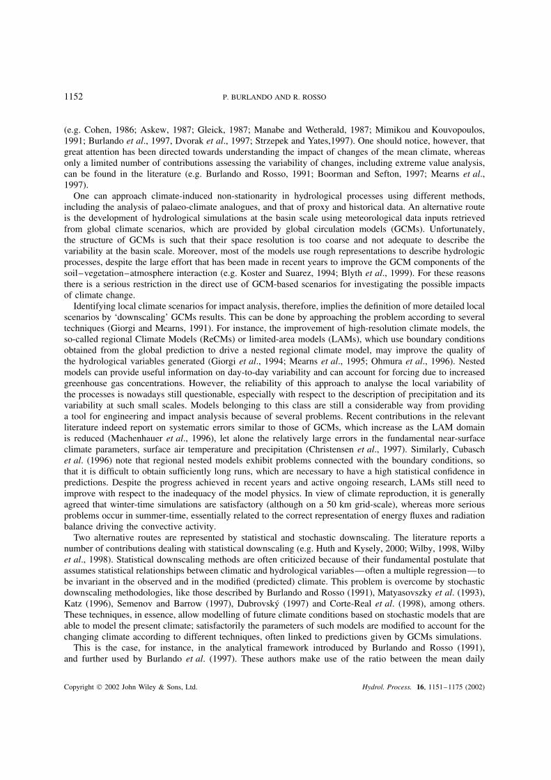
The approach used by Burlando and Rosso (1991) to derive precipitation scenarios at the local and basinscales from GCM outputs is based on stochastic modelling of temporal precipitation using a physically basedrepresentation of the major features of the underlying process. Poisson cluster models give a representation ofthese features as reflected by storm cell dynamics, the statistical properties of which are represented by modelvariates, such as the duration, temporal displacement and rain rate of a cell, and the rate of occurrence of cellclusters and their temporal displacement. An example of cluster model is the Neyman–Scott rectangular pulses(NSRP) model illustrated in Figure 1, which has been shown capable of capturing the observed statisticalproperties of both continuous rainfall and rainfall extremes for a wide range of climate conditions (e.g.Burlando, 1989; Cowpertwait, 1991, 1994, 1995; Burlando and Rosso, 1993; Cowpertwait et al., 1996a, b).For the specific area analysed by the present investigation, the NSRP model has been shown to match themain rainfall characteristics, thereby including statistical, scaling and extreme properties over the period1962–86 (Burlando and Rosso, 1993; Olsson and Burlando, 2002). Under the assumption of a stationaryrainfall process, one can then derive model parameters using the observed precipitation series and matchingthe model-computed statistics with the observed. These are often derived by aggregating the process atdifferent temporal scales in order to achieve a robust model, which is capable of representing the statisticalproperties of precipitation processes over a range of temporal scales. Because cluster dependence shouldreflect seasonal variability, one must introduce a time-dependent (periodic) model parameterization, whichmakes use of statistics on a monthly basis, in order to capture the annual precipitation patterns (e.g. Burlandoand Rosso, 1993). The persistence of wet and dry periods may affect the statistical properties of the observedprocess, thus resulting in different parameter estimates, which then reflect the non-stationary character ofprecipitation rates. In this respect, the NSRP model used in the analysis is briefly reviewed below.

The NSRP model of temporal rainfall

Let X�t� denote rainfall rate at a point in space and time t. The NSRP model is based on Poisson arrivalsof storms, a cluster of rectangular pulses or cells of random height and duration that are randomly displaced

w2

rain

fall

inte

nsity

wj wj+1w1

x(t)

wj = interarrival time of events (pulses)ti

(1) = displacement of the j-th cell from the cluster centertc1

= duration of the i-th pulseic1

= intensity of the i-th pulse

00 t1 tj t

time

t3(1) t2

(1)

t1(1)

t2(1)

t1(1)

tc1

ic

Figure 1. Sketch of the NSRP model of point precipitation



from the cluster origin being associated with each arrival. The superposition of these pulses provides thedescription of the storm profile. It is often assumed that both the intensity and the duration of a pulse areindependent and identically distributed with exponential marginals, being displaced from the cluster originaccording to an exponential distribution, and the number of cells assumed to follow a geometric distribution.The second-order properties of the aggregated process XT�t� at scale T were derived under these assumptionsby Rodriguez-Iturbe (1986), resulting in

E[XT�t�] D ��υ�T �1�

var[XT�t�] D 2��2υ3�

(T

υ� 1 C exp

(�T

υ

))[2 � ˇ2υ2�� 1�

1 � ˇ2υ2

]

C 2��2υ2�� 1�

ˇ�1 � ˇ2υ2�[ˇT � 1 C exp��ˇT�] �2�

cov[XiT, XiCk

T ] D ��2υ3�

[2 � ˇ2υ2�� 1�

1 � ˇ2υ2

] [1 � exp

(�T

υ

)]2

exp[�T�k � 1�

υ

]

C ��2υ2�� 1�

ˇ�1 � ˇ2υ2�[1 � exp��ˇT�]2 exp[�ˇ�k � 1�T]k ½ 1 �3�

where � is the Poisson rate of storm arrival, � and υ are respectively the mean intensity and the mean durationof a pulse, � is the mean number of cells in a cluster, and ˇ�1 is the mean displacement of a cell from thecluster origin. The scale of fluctuation � of the process X�t�, which provides the time interval required toobtain stable (low variance) estimates of the mean of the fluctuating process of rainfall intensity, can beexpressed as

� D 2υ�� C 1�

2 C �� 1�ˇυ

�1 C ˇυ�

�4�

One notes that the scale of fluctuation is independent of the Poisson rate and of the rain rate of a cell, butit is almost equal to twice the average pulse duration for the range of values of υ, ˇ, and � usually found innature.

Downscaling of GCM precipitation outputs using the NSRP model

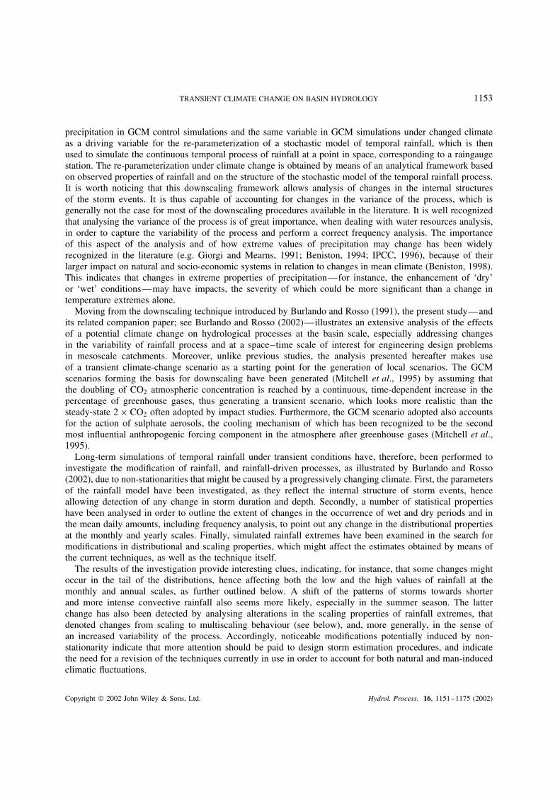
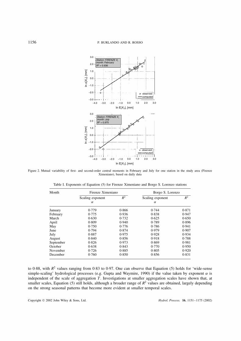
The non-stationary behaviour of precipitation processes is reflected by the statistical properties observed indifferent periods. For example, the second-order statistics of rain rate are expected to vary from one monthto the next. Therefore, one can assume that the process is second-order periodic-stationary, i.e. stationary ina month. However, the average rain rate and its second-order moments in a month of a certain year, e.g. July1998, differ from those observed in the same month of another year, e.g. July 1999. This variability is shownin Figure 2, where the estimated standard deviation sXT�t� is plotted against the estimated mean mXT�t�, ofthe daily precipitation rate at Firenze Ximeniano station in the study area. One can assume that

s2XT�t;�� D b[mXT�t;��]

2˛ �5�

where the scaling exponent ˛ and the constant b can be estimated from the aggregated data of precipitationrate. Here, XT�t; �� denotes aggregated precipitation rate at time t of the �th period of the year, with T denotingthe length of the aggregation window. Figure 2 shows that Equation (5) can reasonably fit the joint variabilityof the observed second-order statistics for the station examined. This assumption is also supported by a largeamount of daily precipitation data in the Arno River basin, as shown in Table I for two stations of the studyarea. The estimated values of the monthly scaling exponent of Equation (5) are found to range from 0Ð73



3.0

2.0

1.0

0.0

−1.0

−2.0

−3.0

−4.0 −3.0 −2.0 −1.0 0.0 1.0 2.0 3.0

−4.0 −3.0 −2.0 −1.0 0.0 1.0 2.0 3.0

Station: FIRENZE Ximonth: FebruaryR2 = 0.936

Station: FIRENZE Ximonth: JulyR2 = 0.975

observedcomputed

observedcomputed

In s

[XT],

[mm

]

3.0

2.0

1.0

0.0

−1.0

−2.0

−3.0

In s

[XT],

[mm

]

In E[XT], [mm]

In E[XT], [mm]

Figure 2. Mutual variability of first- and second-order central moments in February and July for one station in the study area (FirenzeXimeniano), based on daily data

Table I. Exponents of Equation (5) for Firenze Ximeniano and Borgo S. Lorenzo stations

Month Firenze Ximeniano Borgo S. Lorenzo

Scaling exponent R2 Scaling exponent R2

˛ ˛

January 0Ð779 0Ð866 0Ð744 0Ð871February 0Ð775 0Ð936 0Ð838 0Ð947March 0Ð630 0Ð732 0Ð625 0Ð650April 0Ð809 0Ð940 0Ð789 0Ð896May 0Ð750 0Ð776 0Ð786 0Ð941June 0Ð794 0Ð874 0Ð979 0Ð907July 0Ð887 0Ð975 0Ð928 0Ð934August 0Ð840 0Ð856 0Ð918 0Ð788September 0Ð826 0Ð973 0Ð869 0Ð981October 0Ð638 0Ð843 0Ð770 0Ð950November 0Ð726 0Ð885 0Ð805 0Ð920December 0Ð760 0Ð850 0Ð856 0Ð831

to 0Ð88, with R2 values ranging from 0Ð83 to 0Ð97. One can observe that Equation (5) holds for ‘wide-sensesimple-scaling’ hydrological processes (e.g. Gupta and Waymire, 1990) if the value taken by exponent ˛ isindependent of the scale of aggregation T. Investigations at smaller aggregation scales have shown that, atsmaller scales, Equation (5) still holds, although a broader range of R2 values are obtained, largely dependingon the strong seasonal patterns that become more evident at smaller temporal scales.



If one assumes that the modification in the trend variate is expressed by the ratio Km between the meandaily precipitation of the enhanced CO2 scenario m�nðCO2� and the present climate mean daily precipitationm�control� corresponding to the control scenario:

m�nðCO2�

m�control�D Km �6�

the conjecture that the shape and parameters of Equation (5) do not change under the modified scenario yields

2Y

2X

D K D K2˛m �7�

where, for the sake of simplicity, the index Y stands for the enhanced CO2 scenario and X for the controlone. This implies that the standard deviation of the precipitation rate will be modified by a factor of K˛

m ifthe trend of precipitation changes by a factor of Km.

One can obtain a similar relationship to investigate the variability in the scale of fluctuation. Under thefurther assumption of system linearity, one gets (Vanmarcke, 1983)

2X�X

m2X

D 2Y�Y

m2Y

�8�

which can be used to derive the ratio K� of the scales of fluctuation under modified and control conditions,i.e.

K� D K2�1�˛�m �9�

Accordingly, Equations (6), (7) and (9) provide the framework for rescaling the second-order statistics ofthe precipitation rate as a function of the ratio Km representing the change in the precipitation trend. Becausethe second-order statistics of the NSRP model are a function of the five parameters of the model, one can usethese equations to derive analytical relationships for rescaling three out of five parameters of the stochasticmodel. To this purpose, relationships similar to Equation (5) can be written to relate the changes of some ofthe NSRP model parameters between the present (control) and the enhanced CO2 scenario, thus obtaining

�Y

�XD K�;

�Y

�XD K�;

υY

υXD Kυ �10�

For the two remaining parameters, � and ˇ, it is assumed that the number of cells per cluster is unmodifiedunder the enhanced CO2 scenarios, i.e. K� D 1, and that the mean displacement of cells from the clusterorigin is rescaled with respect to the cell duration, namely according to the power law

ˇY

ˇXD Kˇ D �Kυ�

s �11�

where s is a scaling exponent to be evaluated on the basis of the parameter estimated for the control scenario.By combining the NSRP model second-order statistics, i.e. Equations (1)–(3), with Equations (6), (7)

and (9) one finally obtains, after a few manipulations, the ratios K�, K�, and Kυ as functions of Km, whichis the factor of change in the trend of precipitation as provided by GCMs outputs, in the form

K� D Km

K�Kυ�12�

K� D K2˛�1m

Kυ

�1 C 2�

�3 C 4��13�

Kυ D 1 C K�sC1�υ ˇXυX

2 C K�sC1�υ ˇXυX�� C 1�

� K2�1�˛�m

�1 C ˇXυX�

2 C ˇXυX�� C 1��14�



where the mean pulse duration computed for the present scenario υX, the scale of temporal aggregation T,and the scaling factor ˛ are the parameters used for model rescaling, and 1, 2, 3 and 4 are functionsof υX, �, ˇX and T. These are given by

1 D{

υX

[2 � ˇ2

Xυ2X�� 1�

�1 � ˇ2Xυ2

X�

] [T

υX� 1 C exp

(� T

υX

)]}�15�

2 D �� 1�

ˇX�1 � ˇXυX�[ˇX � 1 C exp��ˇXT�] �16�

3 D{

KυυX

[2 � K2�mC1�

υ ˇ2Xυ2

X�� 1�

�1 � K2�mC1�υ ˇ2

Xυ2X�

] [T

KυυX� 1 C exp

(� T

KυυX

)]}�17�

4 D �� 1�

Kmυ ˇX�1 � KmC1

υ ˇXυX�[Km

υ ˇXT � 1 � exp��Kmυ ˇXT�] �18�

After the ratio of change in the precipitation trend Km is obtained from the analysis of the GCM meandaily precipitation totals as averaged on a monthly basis, it is straightforward to estimate the new NSRPparameterization for the n ð CO2 scenario from Equations (11)–(14).

One can observe that this technique limits to the minimum the propagation of GCM errors, which are wellrecognized to be affected by substantial problems with respect to direct simulation of hydrological variables,as clarified in the above sections. This is as a result of the ratio being computed between two homogeneousvariables that are affected by the same bias because they have been computed by the same model. This ratio,and not the mean daily rainfall predicted by GCMs, is used to rescale the historical mean daily rainfall ascomputed from an observed series into a value that is assumed to represent the mean daily rainfall potentially‘measured’ in a changed climate. In other words, it is assumed that the ratio between the observed meandaily rainfall and the mean daily rainfall that is expected to occur under climate change is characterized bythe same ratio computed on the basis of the values predicted by GCMs in the control simulation and in theCO2-enhanced simulation respectively. Although it is recognized that this is an assumption, it must also beobserved that, in practice, the assessment of its validity, and of the validity of any other assumption based onGCM simulation of the recent climate, is not particularly easy because of the uncertainties associated withthe emission scenarios that underlie GCMs predictions.

PRECIPITATION SCENARIOS FOR THE ARNO RIVER BASIN

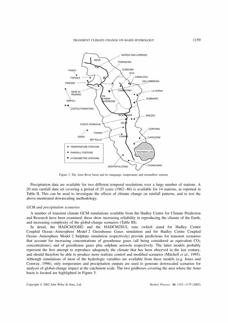
The geographical area selected to perform the analysis of the impact of a potential climate change onprecipitation, and then on rainfall-driven processes (Burlando and Rosso, 2002), is the Arno River basin. Alarge set of historical data is available for the Arno River basin, including both fine resolution and daily rainfallrecords and daily temperature data for a considerable number of stations (Figure 3). Also, daily streamflowand peak flood discharge records are available, thus allowing a detailed simulation of the hydrologic processat different space and time scales.

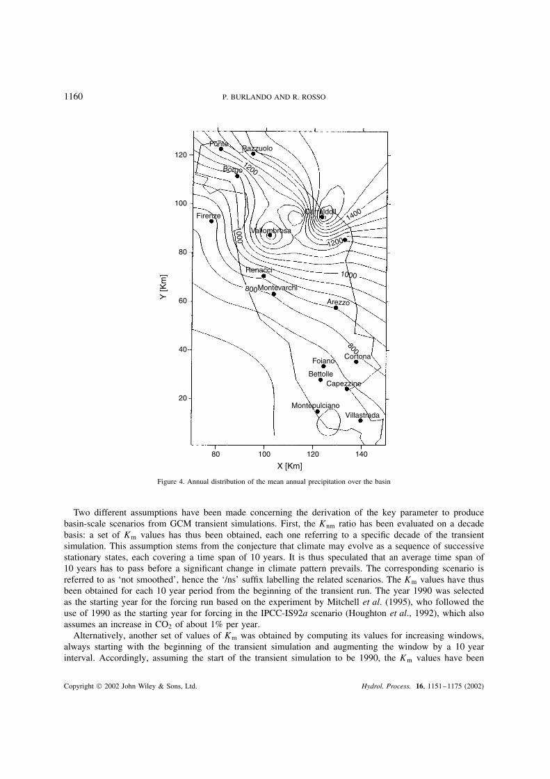
The basin is representative of a Mediterranean climate, with a total annual precipitation from about 700 to1700 mm (Figure 4), and is therefore located in one of the regions that are expected to suffer significantly froma global change. Heavy storms mainly occur in autumn, following dry summers. The mixture of mountainousand flat areas offers a good opportunity to test global-change effects at different elevations and for differentlocal climatic patterns. The mean monthly distribution for summer and autumn precipitation clearly denotesthat the analysis of the potential climate-change impacts is important not only for floods, but also in view ofthe potential increase in summer dryness leading to a water shortage, which is already sometimes a problemin the current climate. A broader description of the Arno River basin is provided in Burlando and Rosso(2002).



BORGO SAN LORENZO

FORNACINA

CONSUMA

STIA

CAMALDOLI

VALLOMBROSA

LA VERNA

SUBBIANO

AREZZO

CORTONA

CAPEZZINE

TRASTMENO LAKE

CHIANCIANOMONTEPULCIANO

TEMPERATURE STATIONS

RAINFALL STATIONS

HYDROMETRIC STATIONS

BETTOLLE

FOIANO

SIENA

PONTE FERROVIA

CASTELFIORENTINO

EMPOLI

NAVE DIROSANO

FIRENZE

FIESOLE

PRATO

SIEVE

VALD'ARNOSUPERIORE

INTERBASIN

VALDI

CHIANA

CASENTINO

Figure 3. The Arno River basin and its raingauge, temperature and streamflow stations

Precipitation data are available for two different temporal resolutions over a large number of stations. A20 min rainfall data set covering a period of 25 years (1962–86) is available for 14 stations, as reported inTable II. This can be used to investigate the effects of climate change on rainfall patterns, and to test theabove-mentioned downscaling methodology.

GCM and precipitation scenarios

A number of transient climate GCM simulations available from the Hadley Centre for Climate Predictionand Research have been examined; these show increasing reliability in reproducing the climate of the Earth,and increasing complexity of the global-change scenarios (Table III).

In detail, the HADCM2GHG and the HADCM2SUL runs (which stand for Hadley CentreCoupled Ocean–Atmosphere Model 2 Greenhouse Gases simulation and for Hadley Centre CoupledOcean–Atmosphere Model 2 Sulphate simulation respectively) provide predictions for transient scenariosthat account for increasing concentrations of greenhouse gases (all being considered as equivalent CO2

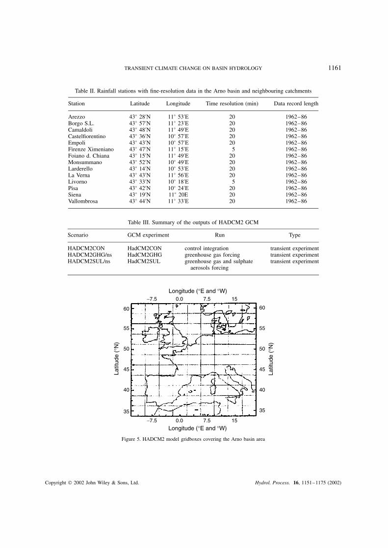
concentrations), and of greenhouse gases plus sulphate aerosols respectively. The latter models probablyrepresent the first attempt to reproduce adequately the climate that has been observed in the last century,and should therefore be able to produce more realistic control and modified scenarios (Mitchell et al., 1995).Although simulations of most of the hydrologic variables are available from these models (e.g. Jones andConway, 1996), only temperature and precipitation outputs are used to generate downscaled scenarios foranalysis of global-change impact at the catchment scale. The two gridboxes covering the area where the Arnobasin is located are highlighted in Figure 5.



1400

1200

Carraldoll

Vallombrosa

Renacci

800Montevarchi

Arezzo1000

Firenze

Borgo1200

PonteRazzuolo

800

CortonaFoiano

BettolleCapezzine

MontepulcianoVillastrada

80 100 120 140

20

40

60

80

100

120

X [Km]

Y [K

m] 1000

Figure 4. Annual distribution of the mean annual precipitation over the basin

Two different assumptions have been made concerning the derivation of the key parameter to producebasin-scale scenarios from GCM transient simulations. First, the Knm ratio has been evaluated on a decadebasis: a set of Km values has thus been obtained, each one referring to a specific decade of the transientsimulation. This assumption stems from the conjecture that climate may evolve as a sequence of successivestationary states, each covering a time span of 10 years. It is thus speculated that an average time span of10 years has to pass before a significant change in climate pattern prevails. The corresponding scenario isreferred to as ‘not smoothed’, hence the ‘/ns’ suffix labelling the related scenarios. The Km values have thusbeen obtained for each 10 year period from the beginning of the transient run. The year 1990 was selectedas the starting year for the forcing run based on the experiment by Mitchell et al. (1995), who followed theuse of 1990 as the starting year for forcing in the IPCC-IS92a scenario (Houghton et al., 1992), which alsoassumes an increase in CO2 of about 1% per year.

Alternatively, another set of values of Km was obtained by computing its values for increasing windows,always starting with the beginning of the transient simulation and augmenting the window by a 10 yearinterval. Accordingly, assuming the start of the transient simulation to be 1990, the Km values have been



Table II. Rainfall stations with fine-resolution data in the Arno basin and neighbouring catchments

Station Latitude Longitude Time resolution (min) Data record length

Arezzo 43° 280N 11° 530E 20 1962–86Borgo S.L. 43° 570N 11° 230E 20 1962–86Camaldoli 43° 480N 11° 490E 20 1962–86Castelfiorentino 43° 360N 10° 570E 20 1962–86Empoli 43° 430N 10° 570E 20 1962–86Firenze Ximeniano 43° 470N 11° 150E 5 1962–86Foiano d. Chiana 43° 150N 11° 490E 20 1962–86Monsummano 43° 520N 10° 490E 20 1962–86Larderello 43° 140N 10° 530E 20 1962–86La Verna 43° 430N 11° 560E 20 1962–86Livorno 43° 330N 10° 180E 5 1962–86Pisa 43° 420N 10° 240E 20 1962–86Siena 43° 190N 11° 20E 20 1962–86Vallombrosa 43° 440N 11° 330E 20 1962–86

Table III. Summary of the outputs of HADCM2 GCM

Scenario GCM experiment Run Type

HADCM2CON HadCM2CON control integration transient experimentHADCM2GHG/ns HadCM2GHG greenhouse gas forcing transient experimentHADCM2SUL/ns HadCM2SUL greenhouse gas and sulphate

aerosols forcingtransient experiment

60

55

50

45

35

40

60

55

50

45

35

40

−7.5 0.0 7.5 15

−7.5 0.0 7.5 15

Longitude (°E and °W)

Latit

ude

(°N

)

Latit

ude

(°N

)

Longitude (°E and °W)

Figure 5. HADCM2 model gridboxes covering the Arno basin area



obtained for the periods 1990–99, 1990–2009, and so on up to the last 10 year increase, yielding an averagingperiod from 1990 to 2099. This second criterion provides a smoothing of the fluctuations determined by thisforcing (hence, the suffix ‘/s’, standing for ‘smoothed’, that labels the corresponding scenarios). Although thismay be questionable, it is conjectured that nature will partially smooth the forcing due to climate change,for instance, by compensating the richer CO2 atmosphere with the enhancement of vegetation activity and,therefore, increasing the magnitude of CO2 sinks.

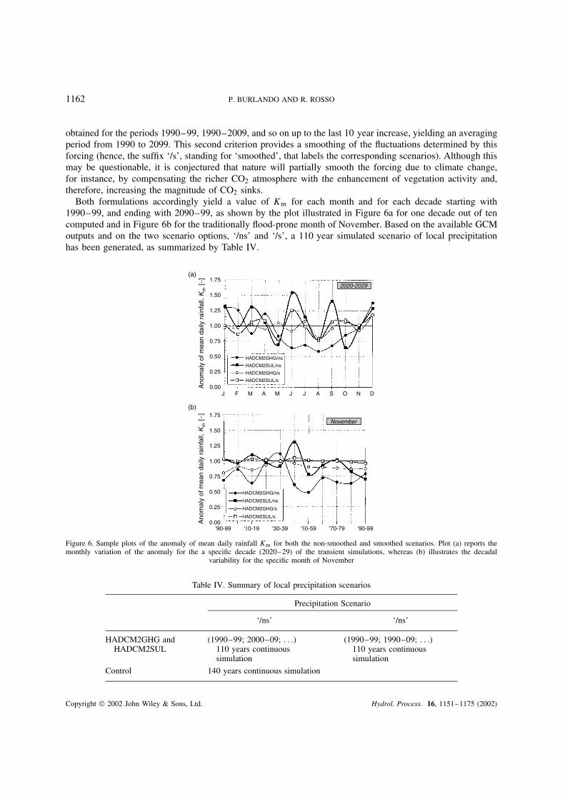
Both formulations accordingly yield a value of Km for each month and for each decade starting with1990–99, and ending with 2090–99, as shown by the plot illustrated in Figure 6a for one decade out of tencomputed and in Figure 6b for the traditionally flood-prone month of November. Based on the available GCMoutputs and on the two scenario options, ‘/ns’ and ‘/s’, a 110 year simulated scenario of local precipitationhas been generated, as summarized by Table IV.

1.75

1.50

1.25

1.00

0.75

0.50

0.25

0.00

HADCM2GHG/ns

HADCM2SUL/ns

HADCM2GHG/s

HADCM2SUL/s

HADCM2GHG/ns

HADCM2SUL/ns

HADCM2GHG/s

HADCM2SUL/s

(a)

(b)

J F M A M J J A S O N D

Ano

mal

y of

mea

n da

ily r

ainf

all,

Km

[−]

1.75

1.50

1.25

1.00

0.75

0.50

0.25

0.00Ano

mal

y of

mea

n da

ily r

ainf

all,

Km

[−]

'90-99 '10-19 '30-39 '50-59 '70-79 '90-99

2020-2029

November

Figure 6. Sample plots of the anomaly of mean daily rainfall Km for both the non-smoothed and smoothed scenarios. Plot (a) reports themonthly variation of the anomaly for the a specific decade (2020–29) of the transient simulations, whereas (b) illustrates the decadal

variability for the specific month of November

Table IV. Summary of local precipitation scenarios

Precipitation Scenario

‘/ns’ ‘/ns’

HADCM2GHG andHADCM2SUL

(1990–99; 2000–09; . . .)110 years continuoussimulation

(1990–99; 1990–09; . . .)110 years continuoussimulation

Control 140 years continuous simulation



THE EXPECTED IMPACT ON RAINFALL REGIME

Internal structure of rainfall events

One of the advantages of the NSRP model technique for the downscaling of GCM precipitation outputsstems from the capability of the stochastic model to perform continuous simulations of the temporal rainfallprocess. This makes an investigation of the internal structure of rainfall events possible, thereby providing aninsight into possible structural changes involved in the modification of rainfall patterns. These modificationsare described by the changes detected in the component variates under the new scenario, as reflected bymodified parameters of the NSRP model.

The results obtained for the transient scenarios benefit from GCM predictions that provide controlsimulations closer to the actual climate than those of the previous generation of models (e.g. Mitchellet al., 1995). Accordingly, the re-parameterization for both the HADCM2GHG and the HADCM2SULscenarios, and for both the ‘/ns’ and ‘/s’ schemes, provides a heterogeneous impact on rainfall pattern,rather than a generalized reduction of rainfall amounts and occurrences as usually retrieved from climatemodels and predicted by most steady-state (2 ð CO2) simulations. As expected, rainfall patterns under theHADCM2GHG/s and HADCM2SUL/s scenarios generally display a smoother response to climate changethan under the ‘/ns’ scenarios, thereby somehow limiting the quantitative impact of climate change, but notmodifying its general trend.

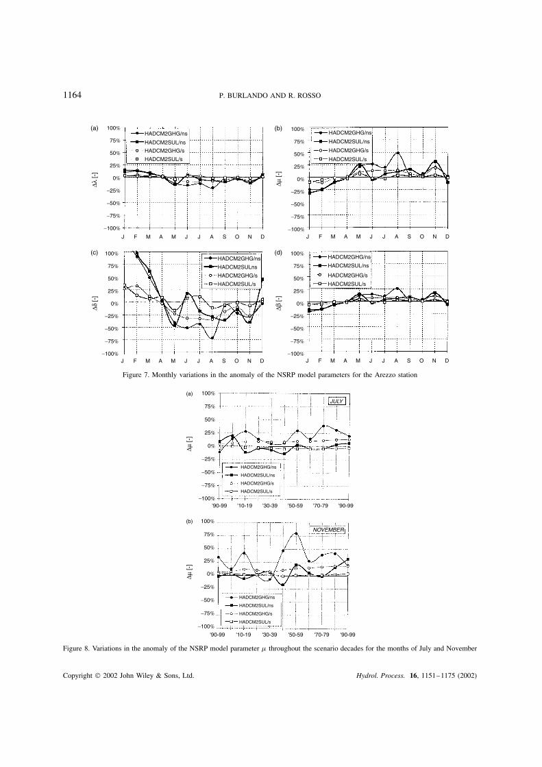
In detail, the mean number of events � displays a decrease in the summer and autumn seasons in all ofthe transient scenarios, ranging from a few percent in late spring and early autumn to about 25% reduction inJuly and August (Figure 7a). The number of storm arrivals conversely increases in the winter season (Januaryto March). Only under the HADCM2SUL/s scenario does � exhibit a weak fluctuation around the no-changeline. A reduction of the frequency of the events should therefore be expected, similar to what is foreseenaccording to many predictions referring to stationary 2 ð CO2 scenarios.

The average rainfall rate � of a storm cell and its duration υ are affected by a dual impact, as shownin Figure 7b and c, illustrating that � increases and υ decreases in spring, summer and autumn, therebystrengthening the hypothesis of an increase in the frequency of short but intense rainfall events throughoutmost of the year, including those seasons that are already characterized by a proneness to flood events. Winterevents should conversely be characterized by a strengthening of the frontal activities with persistent rainfall,as indicated by the increase in the event arrival rate and of the mean cell duration. This behaviour is moredetectable when the ‘/ns’ scenarios are examined, and when the effect of the greenhouse gases is consideredwithout accounting for the sulphate aerosols influence. The latter will contribute to local short-term cooling ofthe atmosphere and, therefore, to a weakening of convective gradients. It is only under the HADCM2SUL/sscenario that the re-parameterization results in a weak and less significant fluctuation in the mean intensity ofcells around the no-change line. Less significant variations are finally observed for the mean displacement ofcells from the cluster origin ˇ, which increases in spring, summer and early autumn, and decreases in winter(Figure 7d). These anomalies also exhibit a tendency to consolidate the outlined patterns for summer monthsthroughout all of the 110 years of the simulation under transient scenarios. As shown in Figure 8, this effectis stronger for greenhouse gas forcing, and weaker when sulphate aerosols are also considered. Similarly, thetendency is more visible if the ‘/ns’ scenarios are considered. The dual case has been observed for winter andautumn months.

As a result of the above changes in NSRP parameters, the long-term simulations of the downscaledprecipitation process from the transient scenarios examined indicate that, for all of the four scenarios examined,one should expect that both the cluster duration and the number of clusters will reduce for the summer season(see Figure 9). This is a consequence of the expected reduction in the mean duration of a cell and in the meannumber of events. An increase in cluster duration is conversely simulated for the winter season, correspondingto the increase in the cell duration already mentioned, which could lead to an increase in high-frequency flood



100%

75%

50%

25%

0%

−25%

−50%

−75%

−100%

100%

75%

50%

25%

0%

−25%

−50%

−75%

−100%

100%

75%

50%

25%

0%

−25%

−50%

−75%

−100%

100%

75%

50%

25%

0%

−25%

−50%

−75%

−100%

HADCM2GHG/ns

HADCM2GHG/s

HADCM2SUL/s

HADCM2SUL/ns

HADCM2GHG/ns

HADCM2GHG/s

HADCM2SUL/s

HADCM2SUL/ns

HADCM2GHG/ns

HADCM2GHG/s

HADCM2SUL/s

HADCM2SULns

HADCM2GHG/ns

HADCM2GHG/s

HADCM2SUL/s

HADCM2SUL/ns





∆λ [-

]∆δ

[-]

∆β [-

]∆µ

[-]

(a)

(c) (d)

(b)

Figure 7. Monthly variations in the anomaly of the NSRP model parameters for the Arezzo station

75%

50%

25%

0%

0%

−25%

−50%

−75%

−100%

100%

75%

50%

25%

−25%

−50%

−75%

−100%

100%

HADCM2GHG/ns

HADCM2GHG/s

HADCM2SUL/s

HADCM2SUL/ns

HADCM2GHG/ns

HADCM2GHG/s

HADCM2SUL/s

HADCM2SUL/ns

'90-99 '10-19 '30-39 '50-59 '70-79 '90-99

'90-99 '10-19 '30-39 '50-59 '70-79 '90-99

JULY

NOVEMBER

(b)

(a)

∆µ [-

]∆µ

[-]

Figure 8. Variations in the anomaly of the NSRP model parameter � throughout the scenario decades for the months of July and November



75%

50%

25%

0%

−25%

−50%

−75%

−100%

100%

75%

50%

25%

0%

−25%

−50%

−75%

−100%

100%

HADCM2GHG/ns

HADCM2GHG/s

HADCM2SUL/s

HADCM2SUL/ns

HADCM2GHG/ns

HADCM2GHG/s

HADCM2SUL/s

HADCM2SUL/ns

Station: AREZZO

Station: AREZZO



∆ cl

uste

r du

ratio

n [-

]∆#

of c

lust

ers

[-]

(a)

(b)

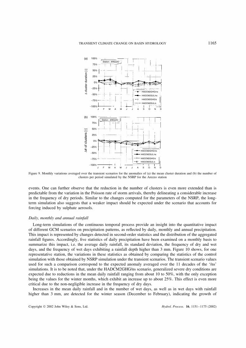
Figure 9. Monthly variations averaged over the transient scenarios for the anomalies of (a) the mean cluster duration and (b) the number ofclusters per period simulated by the NSRP for the Arezzo station

events. One can further observe that the reduction in the number of clusters is even more extended than ispredictable from the variation in the Poisson rate of storm arrivals, thereby delineating a considerable increasein the frequency of dry periods. Similar to the changes computed for the parameters of the NSRP, the long-term simulation also suggests that a weaker impact should be expected under the scenario that accounts forforcing induced by sulphate aerosols.

Daily, monthly and annual rainfall

Long-term simulations of the continuous temporal process provide an insight into the quantitative impactof different GCM scenarios on precipitation patterns, as reflected by daily, monthly and annual precipitation.This impact is represented by changes detected in second-order statistics and the distribution of the aggregatedrainfall figures. Accordingly, five statistics of daily precipitation have been examined on a monthly basis tosummarize this impact, i.e. the average daily rainfall, its standard deviation, the frequency of dry and wetdays, and the frequency of wet days exhibiting a rainfall depth higher than 3 mm. Figure 10 shows, for onerepresentative station, the variations in these statistics as obtained by comparing the statistics of the controlsimulation with those obtained by NSRP simulation under the transient scenarios. The transient scenario valuesused for such a comparison correspond to the expected anomaly averaged over the 11 decades of the ‘/ns’simulations. It is to be noted that, under the HADCM2GHG/ns scenario, generalized severe dry conditions areexpected due to reductions in the mean daily rainfall ranging from about 10 to 50%, with the only exceptionbeing the values for the winter months, which exhibit an increase up to about 25%. This effect is even morecritical due to the non-negligible increase in the frequency of dry days.

Increases in the mean daily rainfall and in the number of wet days, as well as in wet days with rainfallhigher than 3 mm, are detected for the winter season (December to February), indicating the growth of



100%

75%

50%

25%

0%

−25%

−50%

−75%

−100%

100%

75%

50%

25%

0%

−25%

−50%

−75%

−100%

100%

75%

50%

25%

0%

−25%

−50%

−75%

−100%

100%

75%

50%

25%

0%

−25%

−50%

−75%

−100%

100%

75%

50%

25%

0%

−25%

−50%

−75%

−100%






HADCM2GHG/ns

HADCM2SUL/ns

HADCM2GHG/ns

HADCM2SUL/ns

HADCM2GHG/ns

HADCM2SUL/ns

HADCM2GHG/ns

HADCM2SUL/ns

HADCM2GHG/ns

HADCM2SUL/ns

Station: AREZZO Station: AREZZO

Station: AREZZOStation: AREZZO

Station: AREZZO

∆ m

ean

daily

rai

nfal

l [m

m]

∆ va

rianc

e of

dai

ly r

ainf

all [

mm

]

∆ fr

eque

ncy

of d

ry d

ays

[-]

∆ fr

eque

ncy

of w

et d

ays

[-]

∆ fr

eque

ncy

of w

et d

ays,

H>

3 m

m [-

]

(a)

(c)

(e)

(d)

(b)

Figure 10. Station Arezzo, HADCM2GHG/ns scenario. Monthly variations averaged over the transient scenarios for the basic statistics ofdaily rainfall: (a) mean, (b) variance, (c) frequency of dry days, (d) frequency of wet days, (e) frequency of days with rainfall depth >3 mm

potentially high-flow periods in the winter season. Figure 10 also suggests that the results from the NSRPmodel parameterized from the transient scenario HADCM2SUL/ns provide a weaker impact than thosecoming from HADCM2GHG/ns climate simulations. The impact due to greenhouse gases is weakened ifthe sulphate aerosols are included (HADCM2SUL/ns), and when the smoothed scenarios (HADCM2GHG/sand HADCM2SUL/s) are considered. In the case of sulphate-aerosol simulations, the modification of the meandaily rainfall, as well as of the frequency of wet days, is distinctly reduced, as shown in Figure 10. Further,it is worth noticing that the predicted variation in the frequency of wet days in November practically equalsthe increase of the frequency of days characterized by rainfall depths higher than 3 mm; this indicates that ahigher frequency of high flows could be expected for this specific season, which is already recognized as apotential flood period for this area in the present climate.



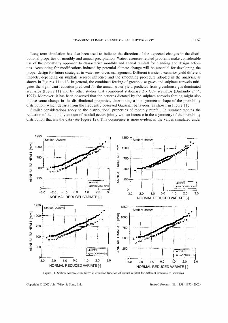
Long-term simulation has also been used to indicate the direction of the expected changes in the distri-butional properties of monthly and annual precipitation. Water-resources-related problems make considerableuse of the probability approach to characterize monthly and annual rainfall for planning and design activi-ties. Accounting for modifications induced by potential climate change will be essential for developing theproper design for future strategies in water resources management. Different transient scenarios yield differentimpacts, depending on sulphate aerosol influence and the smoothing procedure adopted in the analysis, asshown in Figures 11 to 13. In general, the combined forcing of greenhouse gases and sulphate aerosols miti-gates the significant reduction predicted for the annual water yield predicted from greenhouse-gas-dominatedscenarios (Figure 11) and by other studies that considered stationary 2 ð CO2 scenarios (Burlando et al.,1997). Moreover, it has been observed that the patterns dictated by the sulphate aerosols forcing might alsoinduce some change in the distributional properties, determining a non-symmetric shape of the probabilitydistribution, which departs from the frequently observed Gaussian behaviour, as shown in Figure 11c.

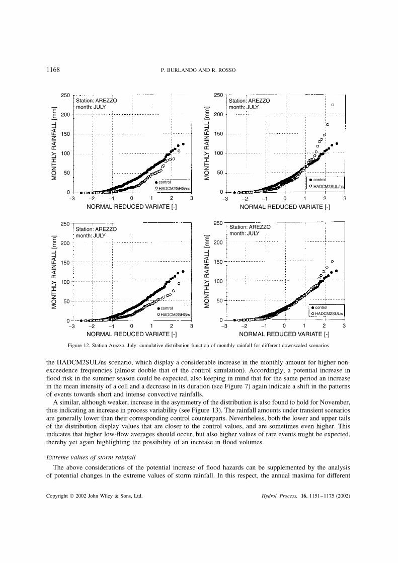
Similar considerations apply to the distributional properties of monthly rainfall. In summer months thereduction of the monthly amount of rainfall occurs jointly with an increase in the asymmetry of the probabilitydistribution that fits the data (see Figure 12). This occurrence is more evident in the values simulated under

1250

1000

750

500

250

0

1250

1000

750

500

250

0

1250

1000

750

500

250

0

1250

1000

750

500

250

0

−3.0 −2.0 −1.0 0.0 1.0 2.0 3.0

−3.0 −2.0 −1.0 0.0 1.0 2.0 3.0 −3.0 −2.0 −1.0 0.0 1.0 2.0 3.0

−3.0 −2.0 −1.0 0.0 1.0 2.0 3.0

Station: Arezzo Station: Arezzo

Station: ArezzoStation: Arezzo

NORMAL REDUCED VARIATE [-]

NORMAL REDUCED VARIATE [-] NORMAL REDUCED VARIATE [-]


AN

NU

AL

RA

INFA

LL [m

m]

AN

NU

AL

RA

INFA

LL [m

m]

AN

NU

AL

RA

INFA

LL [m

m]

AN

NU

AL

RA

INFA

LL [m

m]

control

HADCM2GHG/ns

control

HADCM2GHG/s

control

HADCM2SUL/ns

control

HADCM2SUL/s

Figure 11. Station Arezzo: cumulative distribution function of annual rainfall for different downscaled scenarios



250

200

150

100

50

0

250

200

150

100

50

0

250

200

150

100

50

0

250

200

150

100

50

0−3 −2 −1 0 1 2 3

−3 −2 −1 0 1 2 3 −3 −2 −1 0 1 2 3

−3 −2 −1 0 1 2 3



MO

NT

HLY

RA

INFA

LL [m

m]

MO

NT

HLY

RA

INFA

LL [m

m]

MO

NT

HLY

RA

INFA

LL [m

m]

MO

NT

HLY

RA

INFA

LL [m

m]

control

HADCM2GHG/ns

control

HADCM2SUL/ns

control

HADCM2SUL/scontrol

HADCM2GHG/s

Station: AREZZOmonth: JULY




Figure 12. Station Arezzo, July: cumulative distribution function of monthly rainfall for different downscaled scenarios

the HADCM2SUL/ns scenario, which display a considerable increase in the monthly amount for higher non-exceedence frequencies (almost double that of the control simulation). Accordingly, a potential increase inflood risk in the summer season could be expected, also keeping in mind that for the same period an increasein the mean intensity of a cell and a decrease in its duration (see Figure 7) again indicate a shift in the patternsof events towards short and intense convective rainfalls.

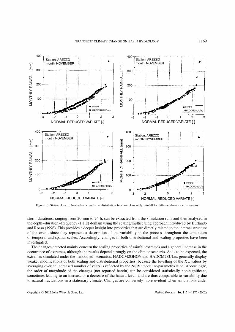
A similar, although weaker, increase in the asymmetry of the distribution is also found to hold for November,thus indicating an increase in process variability (see Figure 13). The rainfall amounts under transient scenariosare generally lower than their corresponding control counterparts. Nevertheless, both the lower and upper tailsof the distribution display values that are closer to the control values, and are sometimes even higher. Thisindicates that higher low-flow averages should occur, but also higher values of rare events might be expected,thereby yet again highlighting the possibility of an increase in flood volumes.

Extreme values of storm rainfall

The above considerations of the potential increase of flood hazards can be supplemented by the analysisof potential changes in the extreme values of storm rainfall. In this respect, the annual maxima for different



400

300

200

100

0

400

300

200

100

0

400

300

200

100

0

−3 −2 −1 0 1 2 3


−3 −2 −1 0 1 2 3

NORMAL REDUCED VARIATE [-]−3 −2 −1 0 1 2 3


control

HADCM2GHG/ns

control

HADCM2GHG/s

Station: AREZZOmonth: NOVEMBER



400

300

200

100

0−3 −2 −1 0 1 2 3


control

HADCM2SUL/ns

control

HADCM2SUL/s


MO

NT

HLY

RA

INFA

LL [m

m]

MO

NT

HLY

RA

INFA

LL [m

m]

MO

NT

HLY

RA

INFA

LL [m

m]

MO

NT

HLY

RA

INFA

LL [m

m]

Figure 13. Station Arezzo, November: cumulative distribution function of monthly rainfall for different downscaled scenarios

storm durations, ranging from 20 min to 24 h, can be extracted from the simulation runs and then analysed inthe depth–duration–frequency (DDF) domain using the scaling/multiscaling approach introduced by Burlandoand Rosso (1996). This provides a deeper insight into properties that are directly related to the internal structureof the event, since they represent a description of the variability in the process throughout the continuumof temporal and spatial scales. Accordingly, changes in both distributional and scaling properties have beeninvestigated.

The changes detected mainly concern the scaling properties of rainfall extremes and a general increase in theoccurrence of extremes, although the results depend strongly on the climate scenario. As is to be expected, theextremes simulated under the ‘smoothed’ scenarios, HADCM2GHG/s and HADCM2SUL/s, generally displayweaker modifications of both scaling and distributional properties, because the levelling of the Km values byaveraging over an increased number of years is reflected by the NSRP model re-parametrization. Accordingly,the order of magnitude of the changes (not reported herein) can be considered statistically non-significant,sometimes leading to an increase or a decrease of the hazard level, and are thus comparable to variability dueto natural fluctuations in a stationary climate. Changes are conversely more evident when simulations under



200

150

100

50

0

200

150

100

50

0

200

150

100

50

0

200

150

100

50

01 10 100 1000

1 10 100 1000 1 10 100 1000

1 10 100 1000RETURN PERIOD, R [years]

RETURN PERIOD, R [years] RETURN PERIOD, R [years]

RETURN PERIOD, R [years]

RA

INFA

LL D

EP

TH

[mm

] R

AIN

FALL

DE

PT

H [m

m]

RA

INFA

LL D

EP

TH

[mm

] R

AIN

FALL

DE

PT

H [m

m]

controlHADCM2GHG/ns

controlHADCM2SUL/ns

controlHADCM2SUL/ns

controlHADCM2GHG/nsStation: VALLOMBROSA Station: AREZZO

Station: FIRENZE Station: BORGO S.L

T = 24h

T = 24h

T = 24h

T = 6h

T = 6h

T = 6h

T = 1h

T = 1h

T = 24h

T = 6h

T = 1h

T = 1h

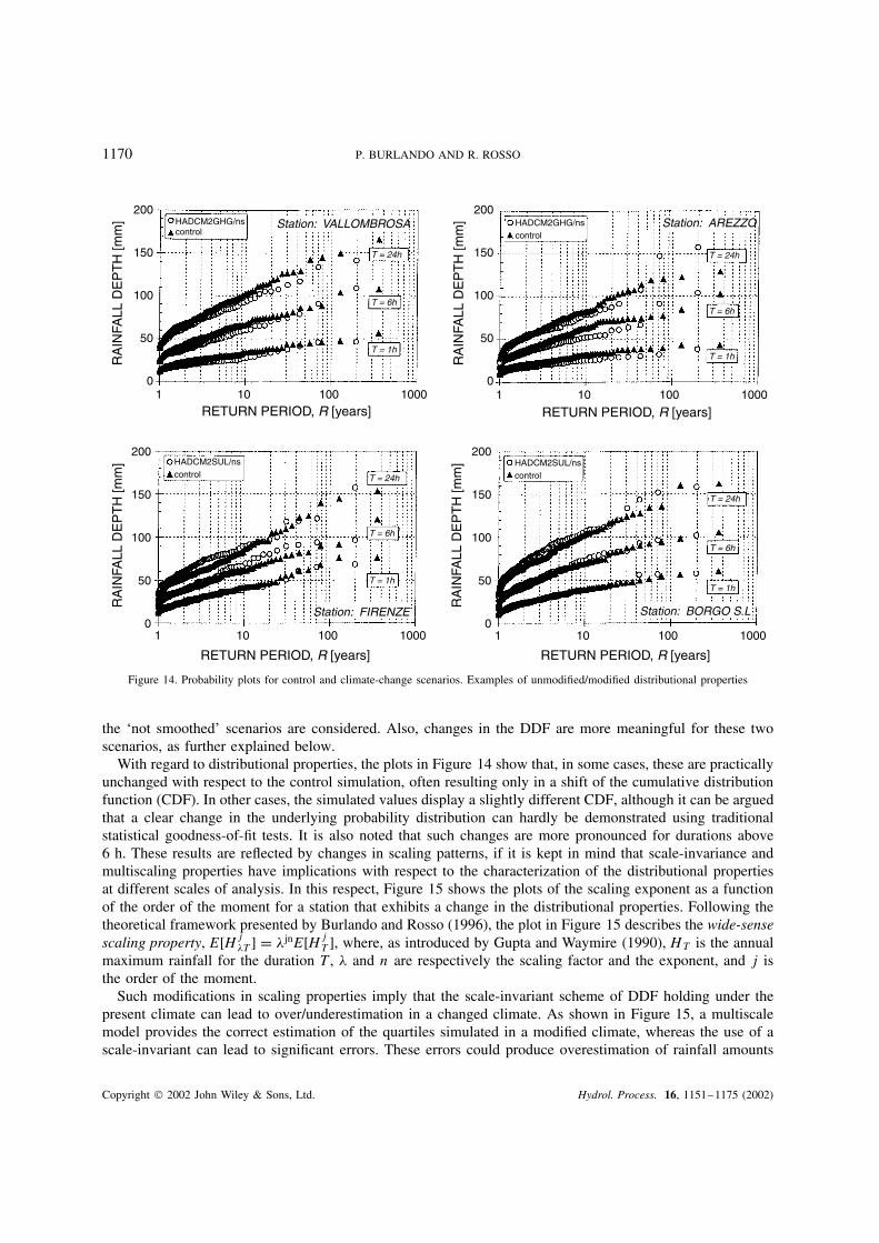
Figure 14. Probability plots for control and climate-change scenarios. Examples of unmodified/modified distributional properties

the ‘not smoothed’ scenarios are considered. Also, changes in the DDF are more meaningful for these twoscenarios, as further explained below.

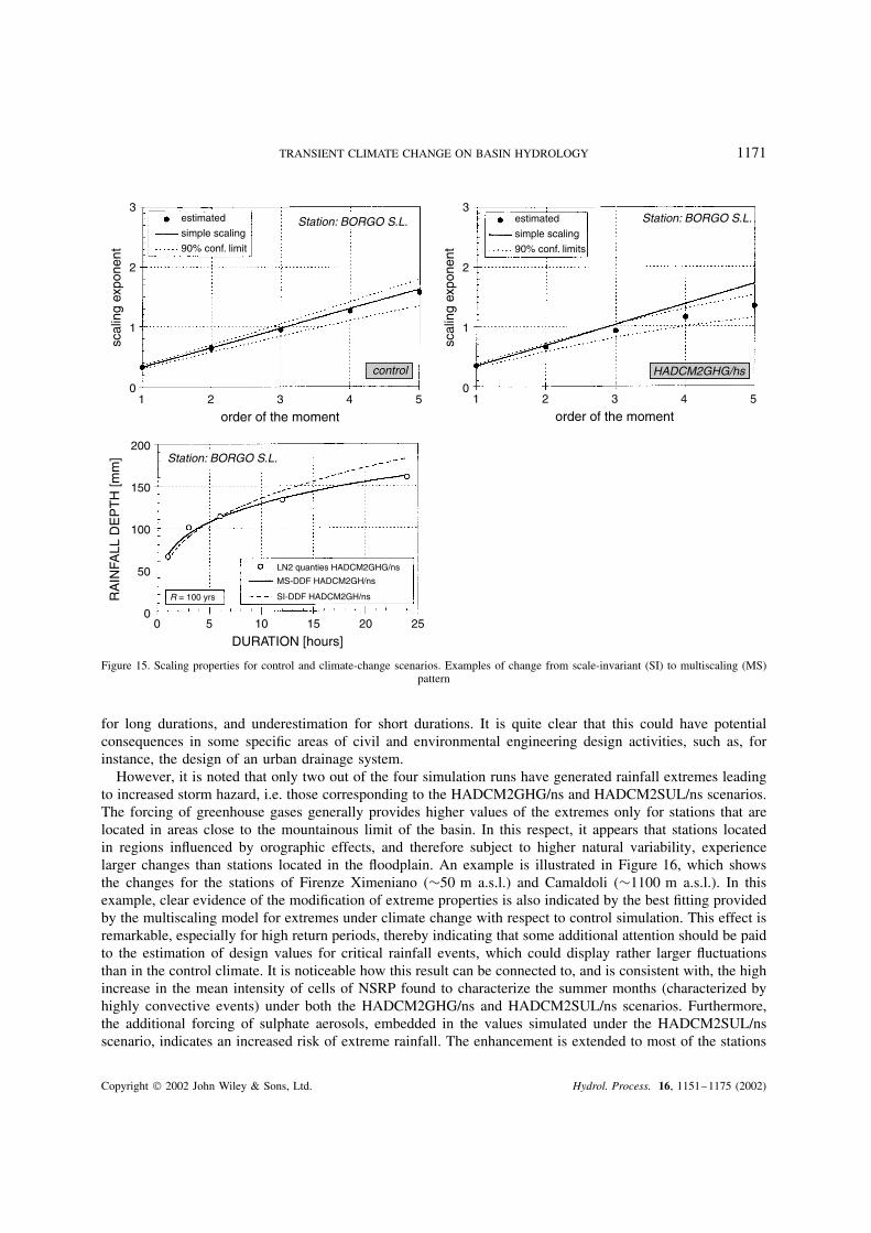
With regard to distributional properties, the plots in Figure 14 show that, in some cases, these are practicallyunchanged with respect to the control simulation, often resulting only in a shift of the cumulative distributionfunction (CDF). In other cases, the simulated values display a slightly different CDF, although it can be arguedthat a clear change in the underlying probability distribution can hardly be demonstrated using traditionalstatistical goodness-of-fit tests. It is also noted that such changes are more pronounced for durations above6 h. These results are reflected by changes in scaling patterns, if it is kept in mind that scale-invariance andmultiscaling properties have implications with respect to the characterization of the distributional propertiesat different scales of analysis. In this respect, Figure 15 shows the plots of the scaling exponent as a functionof the order of the moment for a station that exhibits a change in the distributional properties. Following thetheoretical framework presented by Burlando and Rosso (1996), the plot in Figure 15 describes the wide-sensescaling property, E[Hj

�T] D �jnE[HjT], where, as introduced by Gupta and Waymire (1990), HT is the annual

maximum rainfall for the duration T, � and n are respectively the scaling factor and the exponent, and j isthe order of the moment.

Such modifications in scaling properties imply that the scale-invariant scheme of DDF holding under thepresent climate can lead to over/underestimation in a changed climate. As shown in Figure 15, a multiscalemodel provides the correct estimation of the quartiles simulated in a modified climate, whereas the use of ascale-invariant can lead to significant errors. These errors could produce overestimation of rainfall amounts



3

2

1

1 2 3 4 5

0 5 10 15 20 25

0

200

150

100

50

0

order of the moment1 2 3 4 5

order of the moment

DURATION [hours]

scal

ing

expo

nent

3

2

1

0

scal

ing

expo

nent

RA

INFA

LL D

EP

TH

[mm

]

estimated

simple scaling

90% conf. limit

estimated

simple scaling

90% conf. limits

Station: BORGO S.L. Station: BORGO S.L.

Station: BORGO S.L.

R = 100 yrs

LN2 quanties HADCM2GHG/ns

MS-DDF HADCM2GH/ns

SI-DDF HADCM2GH/ns

control HADCM2GHG/hs

Figure 15. Scaling properties for control and climate-change scenarios. Examples of change from scale-invariant (SI) to multiscaling (MS)pattern

for long durations, and underestimation for short durations. It is quite clear that this could have potentialconsequences in some specific areas of civil and environmental engineering design activities, such as, forinstance, the design of an urban drainage system.

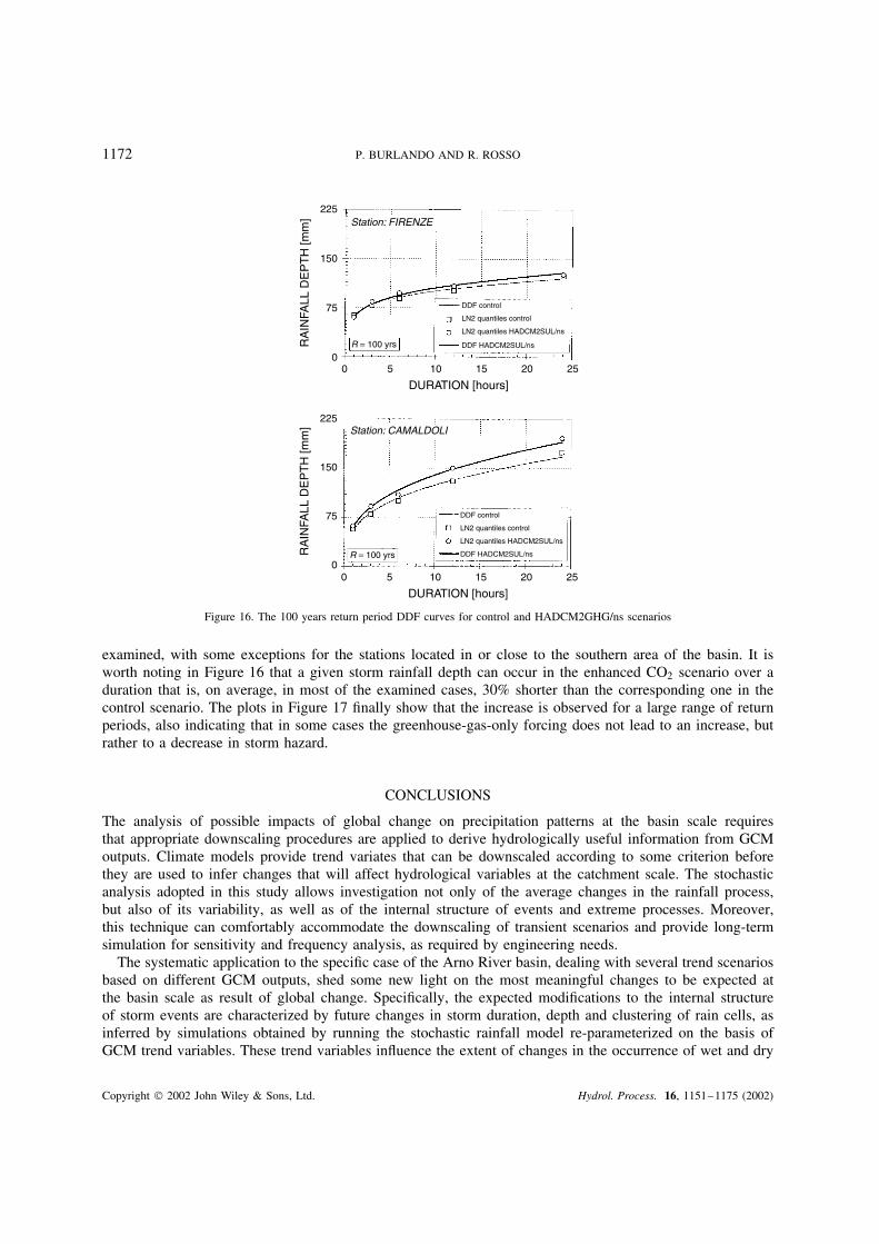
However, it is noted that only two out of the four simulation runs have generated rainfall extremes leadingto increased storm hazard, i.e. those corresponding to the HADCM2GHG/ns and HADCM2SUL/ns scenarios.The forcing of greenhouse gases generally provides higher values of the extremes only for stations that arelocated in areas close to the mountainous limit of the basin. In this respect, it appears that stations locatedin regions influenced by orographic effects, and therefore subject to higher natural variability, experiencelarger changes than stations located in the floodplain. An example is illustrated in Figure 16, which showsthe changes for the stations of Firenze Ximeniano (¾50 m a.s.l.) and Camaldoli (¾1100 m a.s.l.). In thisexample, clear evidence of the modification of extreme properties is also indicated by the best fitting providedby the multiscaling model for extremes under climate change with respect to control simulation. This effect isremarkable, especially for high return periods, thereby indicating that some additional attention should be paidto the estimation of design values for critical rainfall events, which could display rather larger fluctuationsthan in the control climate. It is noticeable how this result can be connected to, and is consistent with, the highincrease in the mean intensity of cells of NSRP found to characterize the summer months (characterized byhighly convective events) under both the HADCM2GHG/ns and HADCM2SUL/ns scenarios. Furthermore,the additional forcing of sulphate aerosols, embedded in the values simulated under the HADCM2SUL/nsscenario, indicates an increased risk of extreme rainfall. The enhancement is extended to most of the stations



225

150

75

00 5 10 15 20 25

Station: FIRENZE

Station: CAMALDOLI

R = 100 yrs

R = 100 yrs

DDF control

DDF HADCM2SUL/ns

LN2 quantiles control

LN2 quantiles HADCM2SUL/ns

DDF control

DDF HADCM2SUL/ns

LN2 quantiles control

LN2 quantiles HADCM2SUL/ns

RA

INFA

LL D

EP

TH

[mm

]

225

150

75

0

RA

INFA

LL D

EP

TH

[mm

]

DURATION [hours]

0 5 10 15 20 25

DURATION [hours]

Figure 16. The 100 years return period DDF curves for control and HADCM2GHG/ns scenarios

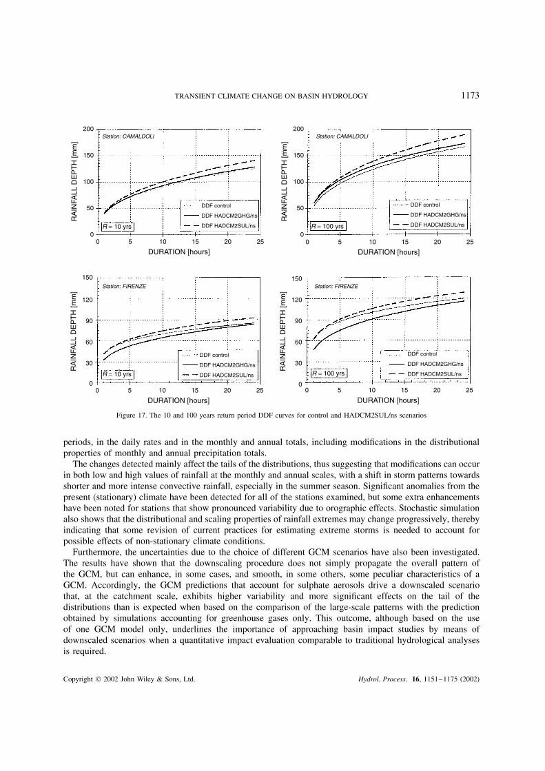
examined, with some exceptions for the stations located in or close to the southern area of the basin. It isworth noting in Figure 16 that a given storm rainfall depth can occur in the enhanced CO2 scenario over aduration that is, on average, in most of the examined cases, 30% shorter than the corresponding one in thecontrol scenario. The plots in Figure 17 finally show that the increase is observed for a large range of returnperiods, also indicating that in some cases the greenhouse-gas-only forcing does not lead to an increase, butrather to a decrease in storm hazard.

CONCLUSIONS

The analysis of possible impacts of global change on precipitation patterns at the basin scale requiresthat appropriate downscaling procedures are applied to derive hydrologically useful information from GCMoutputs. Climate models provide trend variates that can be downscaled according to some criterion beforethey are used to infer changes that will affect hydrological variables at the catchment scale. The stochasticanalysis adopted in this study allows investigation not only of the average changes in the rainfall process,but also of its variability, as well as of the internal structure of events and extreme processes. Moreover,this technique can comfortably accommodate the downscaling of transient scenarios and provide long-termsimulation for sensitivity and frequency analysis, as required by engineering needs.

The systematic application to the specific case of the Arno River basin, dealing with several trend scenariosbased on different GCM outputs, shed some new light on the most meaningful changes to be expected atthe basin scale as result of global change. Specifically, the expected modifications to the internal structureof storm events are characterized by future changes in storm duration, depth and clustering of rain cells, asinferred by simulations obtained by running the stochastic rainfall model re-parameterized on the basis ofGCM trend variables. These trend variables influence the extent of changes in the occurrence of wet and dry



200

150

100

50

00 5 10 15 20 25

R = 10 yrs R = 100 yrs

R = 10 yrs R = 100 yrs

DDF control

DDF HADCM2SUL/ns

DDF HADCM2GHG/ns

DDF control

DDF HADCM2SUL/ns

DDF HADCM2GHG/ns

DDF control

DDF HADCM2SUL/ns

DDF HADCM2GHG/ns

DDF control

DDF HADCM2SUL/ns

DDF HADCM2GHG/ns

Station: CAMALDOLI Station: CAMALDOLI

Station: FIRENZE Station: FIRENZE

RA

INFA

LL D

EP

TH

[mm

]

200

150

100

50

0

RA

INFA

LL D

EP

TH

[mm

]150

120

90

60

30

0

RA

INFA

LL D

EP

TH

[mm

]

150

120

90

60

30

0

RA

INFA

LL D

EP

TH

[mm

]

DURATION [hours]0 5 10 15 20 25

DURATION [hours]

0 5 10 15 20 25

DURATION [hours]

0 5 10 15 20 25

DURATION [hours]

Figure 17. The 10 and 100 years return period DDF curves for control and HADCM2SUL/ns scenarios

periods, in the daily rates and in the monthly and annual totals, including modifications in the distributionalproperties of monthly and annual precipitation totals.

The changes detected mainly affect the tails of the distributions, thus suggesting that modifications can occurin both low and high values of rainfall at the monthly and annual scales, with a shift in storm patterns towardsshorter and more intense convective rainfall, especially in the summer season. Significant anomalies from thepresent (stationary) climate have been detected for all of the stations examined, but some extra enhancementshave been noted for stations that show pronounced variability due to orographic effects. Stochastic simulationalso shows that the distributional and scaling properties of rainfall extremes may change progressively, therebyindicating that some revision of current practices for estimating extreme storms is needed to account forpossible effects of non-stationary climate conditions.

Furthermore, the uncertainties due to the choice of different GCM scenarios have also been investigated.The results have shown that the downscaling procedure does not simply propagate the overall pattern ofthe GCM, but can enhance, in some cases, and smooth, in some others, some peculiar characteristics of aGCM. Accordingly, the GCM predictions that account for sulphate aerosols drive a downscaled scenariothat, at the catchment scale, exhibits higher variability and more significant effects on the tail of thedistributions than is expected when based on the comparison of the large-scale patterns with the predictionobtained by simulations accounting for greenhouse gases only. This outcome, although based on the useof one GCM model only, underlines the importance of approaching basin impact studies by means ofdownscaled scenarios when a quantitative impact evaluation comparable to traditional hydrological analysesis required.



Finally, the above approach provides local precipitation scenarios that are also useful for extensivesimulation of basin water fluxes in the Arno River, as further reported in a companion paper (Burlandoand Rosso, 2002).

ACKNOWLEDGEMENTS

This research work has been supported by the European Union through the POPSICLE project under the IVFramework Programme (contract no. EV5V-CT94-0510). The Hadley Research Centre for Climate Predictionand Research is gratefully acknowledged for allowing the use of the outputs from HADCM2 models. Gratefulthanks are due to Alberto Montanari (DISTART, University of Bologna) for his help in data processing.

REFERENCES

Askew AJ. 1987. Climate change and water resources. In The Influence of Climate Change and Climate Variability on the Hydrologic Regimeand Water Resources , Solomon SI, Beran M, Hogg W (eds). IAHS Publication, Vol. 168. IAHS: Wallingford; 421–430.

Beniston M (ed.). 1994. Mountain Environments in Changing Climates . Routledge Publishing Co.: London.Beniston M. 1998. From Turbulence to Climate. Springer Verlag: Berlin.Blyth EM, Harding RJ, Essery R. 1999. A coupled dual source GCM SVAT. Hydrology and Earth System Sciences 3(1): 71–84.Boorman DB, Sefton CEM. 1997. Recognizing the uncertainty in the quantification of the effects of climate change on hydrological response.

Climatic Change 35: 415–434.Burlando P. 1989. Mathematical models for temporal rainfall simulation and prediction. PhD thesis, Institute of Hydraulics, Politecnico di

Milano, Milan, Italy; (in Italian).Burlando P, Rosso R. 1991. Extreme storm rainfall and climate change. Atmospheric Research 27: 169–189.Burlando P, Rosso R. 1993. Stochastic models of temporal rainfall: reproducibility, estimation and prediction of extreme events. In Stochastic

Hydrology and its Use in Water Resources Systems Simulation and Optimization, Salas JD, Harboe R, Marco-Segura J (eds). KluwerAcademic: Dordrecht, The Netherlands; 137–173.

Burlando P, Rosso R. 1996. Scaling and multiscaling depth–duration–Frequency curves of storm precipitation. Journal of Hydrology187(1–2): 45–64.

Burlando P, Rosso R. 2002. Effects of transient climate change on basin hydrology. 2. Impacts on runoff variability in the Arno River,Central Italy. Hydrological Processes 16: 1177–1199.

Burlando P, Grossi G, Montanari A, Rosso R. 1997. POPSICLE—production of precipitation scenarios for impact assessment of climatechange in Europe. EC Framework III Project RTD EV5V-CT94-0510, Contractor’s Final Report of CIRITA Politecnico di Milano, Milan,Italy.

Christensen JH, Machenhauer B, Jones RG, Schar C, Ruti PM, Castro M, Visconti G. 1997. Validation of present-day regional climatesimulations over Europe: LAM simulations with observed boundary conditions. Climate Dynamics 13: 489–506.

Cohen SJ. 1986. Impacts of CO2-induced climatic change on water resources in the Great Lakes Basin. Climatic Change 8: 135–153.Corte-Real J, Xu H, Qian B. 1998. Downscaling GCM large-scale information to regional climate scenario: a weather generator based on

daily circulation patterns. Annales de Geophysical 16(suppl.): C450.Cowpertwait PSP. 1991. Further developments of the Neyman–Scott clustered point process for modelling rainfall. Water Resources Research

27(7): 1431–1438.Cowpertwait PSP. 1994. A generalized point process model for rainfall. Proceedings of the Royal Society of London, Series A: Mathematics

and Physical Sciences 447: 23–37.Cowpertwait PSP. 1995. A generalized spatial–temporal model of rainfall based on a clustered point process. Proceedings of the Royal

Society of London, Series A: Mathematics and Physical Sciences 450: 163–175.Cowpertwait PSP, O’Connell PE, Metcalfe AV, Mawdsley J. 1996a. Stochastic point process modelling of rainfall. I. Single-site fitting and

validation. Journal of Hydrology 175: 17–46.Cowpertwait PSP, O’Connell PE, Metcalfe AV, Mawdsley J. 1996b. Stochastic point process modelling of rainfall. II. Regionalization and

disaggregation. Journal of Hydrology 175: 47–65.Cubasch U, von Storch H, Waszkewitz J, Zorita E. 1996. Estimates of climate change in southern Europe using different downscaling

techniques. Report No. 183, Max-Plank-Institut fur Meteorologie, Hamburg, Germany.Dubrovsky M. 1997. Creating daily weather series with use of the weather generator. Environmetrics 8: 409–424.Dvorak V, Hladny J, Kasparek L. 1997. Climate change hydrology and water resources impact and adaptation for selected river basins in

the Czech Republic. Climatic Change 36: 93–106.Giorgi F, Mearns LO. 1991. Approaches to the simulation of regional climate change: a review. Reviews of Geophysics 29: 191–216.Giorgi F, Brodeur CS, Bates GT. 1994. Regional climate change scenarios over the United States produced with a nested regional climate

model. Journal of Climate 7: 375–399.Gleick PH. 1987. Global climatic changes and regional hydrology: impacts and responses. In The Influence of Climate Change and Climate

Variability on the Hydrologic Regimes and Water Resources , Solomon SI, Beran M, Hogg W (eds). IAHS Publication, Vol. 168. IAHS:Wallingford; 389–402.



Gupta VK, Waymire E. 1990. Multiscaling properties of spatial rainfall and river flow distributions. Journal of Geophysical Research 95(D3):1999–2009.

Houghton JT, Callander BA, Varney SK (eds). 1992. Climate Change 1992: The Supplementary Report to the IPCC Scientific Assessment .Cambridge University Press: Cambridge; 200 pp.

Huth R, Kysely J. 2000. Constructing site-specific climate change scenarios on a monthly scale using statistical downscaling. Theoreticaland Applied Climatology 66(1–2): 13–27.

IPCC. 1995a. Climate Change 1995: The Science of Climate Change Contribution of Working Group I to the Second Assessment Report ofthe Intergovernmental Panel on Climate Change, Houghton JT, Meiro Filho LG, Callander BA, Harris N, Kattenberg A, Maskell K (eds).Cambridge University Press: 572 pp.

IPCC. 1995b. Climate Change 1995: Impacts, Adaptations and Mitigation of Climate Change: Scientific–Technical Analyses Contributionof Working Group II to the Second Assessment Report of the Intergovernmental Panel on Climate Change, Watson RT, Zinyowera MC,Moss RH (eds). Cambridge University Press: 878 pp.

IPCC. 1995c. Climate Change 1995: Economic and Social Dimensions of Climate Change Contribution of Working Group III to the SecondAssessment Report of the Intergovernmental Panel on Climate Change, Bruce J, Lee H, Haites E (eds). Cambridge University Press:448 pp.

IPCC. 1996. Climate Change. The IPCC Second Assessment Report . Cambridge University Press: Cambridge.IPCC. 1997. The regional impacts of climate change: an assessment of vulnerability, Watson RT, Zinyowera MC, Moss RH, Dokken DJ

(eds). A special report of IPCC Working Group II.Jones PD, Conway D. 1996. POPSICLE—production of precipitation scenarios for impact assessment of climate change in Europe. EC

Framework III Project RTD EV5V-CT94-0510, Contractor’s Final Report, University of East Anglia, Norwich, UK.Katz RW. 1996. Use of conditional stochastic models to generate climate change scenarios. Climatic Change 32(3): 237–255.Koster RD, Suarez MJ. 1994. The components of a SVAT scheme and their effects on a GCMs hydrological cycle. Advances in Water

Resources 17(1–2): 61–78.Machenhauer B, Windelband M, Botzet M, Jones RG, Deque M. 1996. Validation of present-day regional climate simulations over Europe:

nested LAM and variable resolution global model simulations with observed mixed layer ocean boundary conditions. Report No. 191, MaxPlanck Institute for Meteorology, Hamburg, Germany.

Manabe S, Stouffer RJ. 1980. Sensitivity of a global climate model to an increasing the CO2 concentration in the atmosphere. Journal ofAtmospheric Science 37: 99–118.

Manabe S, Wetherald RT. 1987. Large scale changes of soil wetness induced by an increase in atmospheric carbon dioxide. Journal ofAtmospheric Science 44: 1211–1235.

Matyasovszky I, Bogardi I, Bardossy A, Duckstein L. 1993. Space–time precipitation reflecting climate change. Hydrological SciencesJournal 38: 539–558.

Mearns LO, Giorgi F, McDaniel L, Shields C. 1995. Analysis of daily variability of precipitation in a nested regional climatemodel—comparison with observations and doubled CO2 results. Global and Planetary change 10: 55–78.

Mearns LO, Rosenzweig C, Goldberg R. 1997. Mean and variance change in climate scenarios: methods, agricultural applications, andmeasures of uncertainty. Climatic Change 35: 367–396.

Mimikou M, Kouvopoulos YS. 1991. Regional climate change impacts: 1. Impacts on water resources. Hydrological Sciences Journal 36:247–258.

Mitchell JFB, Johns TC, Gregory JM, Tett SFB. 1995. Climate response to increasing levels of greenhouse gases and sulphate aerosols.Nature 376: 501–504.

Nemec J, Schaake JC. 1982. Sensitivity of water resource system to climate variations. Hydrological Sciences Journal 27: 327–343.Ohmura A, Beniston M, Rotach M, Tschuck P, Wild M, Marinucci MR. 1996. Simulation of climate trends over the alpine region. Final

report, Nat. Res. Project 31. Vdf Hochschulverlag AG: Zurich, Switzerland.Olsson J, Burlando P. 2002. Reproduction of temporal scaling by a rectangular pulses rainfall model. Hydrological Processes 16: 611–630.Rodriguez-Iturbe I. 1986. Scale of fluctuation of rainfall models. Water Resources Research 22(9): 15S–37S.Semenov MA, Barrow EM. 1997. Use of stochastic weather generator in the development of climate change scenarios. Climatic Change

35: 397–414.Strzepek KM, Yates D. 1997. Climate change impacts on the hydrologic resources of Europe: a simplified continental scale analysis. Climatic

Change 36: 79–92.Vanmarcke E. 1983. Random fields: analysis and synthesis . MIT Press: Cambridge, MA.Wilby RL. 1998. Statistical downscaling of daily precipitation using daily airflow and seasonal teleconnection indices. Climate Research

10(3): 163–178.Wilby RL, Wigley TML, Conway D, Jones PD, Hewiston BC, Main J, Wilks DS. 1998. Statistical downscaling of general circulation model

output: a comparison of methods. Water Resources Research 34(11): 2995–3008.


Effects of transient climate change on basin hydrology. 1 ...

Documents

Transcript of Effects of transient climate change on basin hydrology. 1 ...