Hydrology of the Upper Malad River Basin, Southeastern Idaho
93
Hydrology of the Upper Malad River Basin, Southeastern Idaho By E. J. PLUHOWSKI GEOLOGICAL SURVEY WATER-SUPPLY PAPER 1888 UNITED STATES GOVERNMENT PRINTING OFFICE, WASHINGTON : 1970
Transcript of Hydrology of the Upper Malad River Basin, Southeastern Idaho

Hydrology of the Upper Malad River Basin, Southeastern IdahoBy E. J. PLUHOWSKI
GEOLOGICAL SURVEY WATER-SUPPLY PAPER 1888
UNITED STATES GOVERNMENT PRINTING OFFICE, WASHINGTON : 1970

UNITED STATES DEPARTMENT OF THE INTERIOR
WALTER J. HIGKEL, Secretary
GEOLOGICAL SURVEY
William T. Pecora, Director
Library of Congress catalog-card No. 73-604793
For sale by the Superintendent of Documents, U.S. Government Printing Office Washington, D.C. 20402 - Price 45 cents
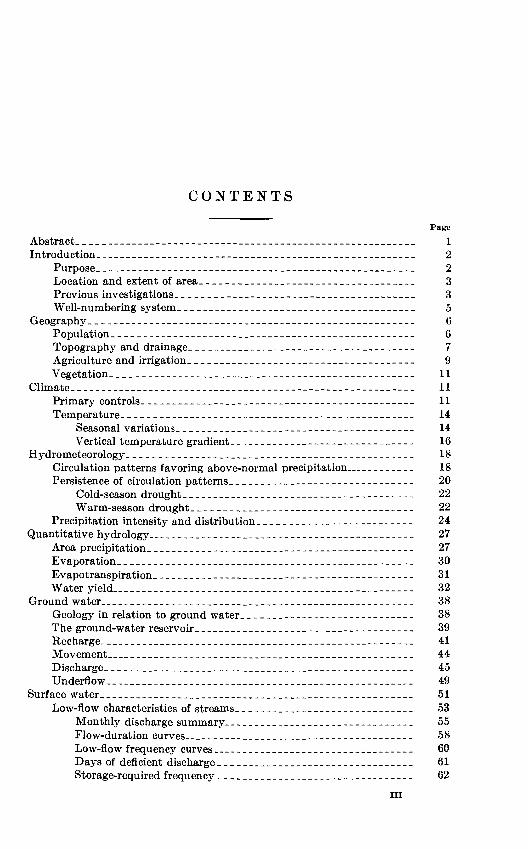
CONTENTS
PageAbstract. _________-__-_-----_-------____-____-___________________ 1Introduction._____________________________________________________ 2
Purpose.___-_-___---------------_---_-_-_---_____________-_-_ 2Location and extent of area.-__-_-__________-_--_-_-_-_________ 3Previous investigations._______________________________________ 3Well-numbering system________________________________________ 5
Geography. ______-_____-_--____-__-__--__-_---_-_-___-____-__-_-- 6Population ___________________________________________________ 6Topography and drainage.____-__________--__-_____-_______---- 7Agriculture and irrigation_________________-__-_-___-___-_------ 9Vegetation. ___-______________-_________-_-_---_-_-___-___---_ 11
Climate._________________-___-_____..__----_---------_------_----- 11Primary controls.____________-__-_-_-___-_---_--____---__---__ 11Temperature. ___________________________-_-----__---_-___--_- 14
Seasonal variations._______________________________________ 14Vertical temperature gradient-____________-----_-------__--- 16
Hydrometeorology _ ____________________________--_-_-_-_-------_-_ 18Circulation patterns favoring above-normal precipitation ________ 18Persistence of circulation patterns.______________________---_--_- 20
Cold-season drought.__________________-__--__--_--------__ 22Warm-season drought_____-_________------------------_-_- 22
Precipitation intensity and distribution__________-___-----_-_--__ 24Quantitative hydrology_____________________-__--_---_--_------_-_ 27
Area precipitation.______-_-_____________-_-_-__--_------------ 27Evaporation.___________________________________ ___---_-__--_ 30Evapotranspiration. _______________________-_-___---_____------ 31Water yield..._.___.___.___._._..___.__._ ________.._._.___.. 32
Ground water_____________________________________________________ 38Geology in relation to ground water.____________________________ 38The ground-water reservoir.______-_______-___-_____------------ 39Recharge. __________-________________________--__-__-_------__ 41Movement__ ________________________________________________ 44Discharge.___________________________________________________ 45Underflow- ____________________________________________________ 49
Surface water.____________________________________________________ 51Low-flow characteristics of streams._____________________________ 53
Monthly discharge summary._______________________________ 55Flow-duration curves__-_----_________-__--___----_--_---- 58Low-flow frequency curves________________________________ 60Days of deficient discharge_____..______________-____--_---- 61Storage-required frequency _________________________________ 62
in
IV CONTENTS
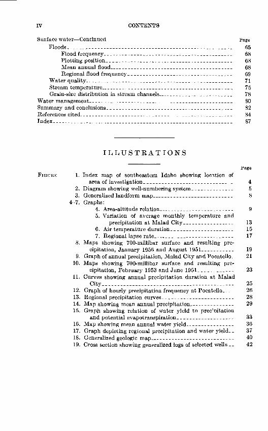
Surface water ContinuedFloods._______________________________
Flood frequency.__________________Plotting position._________________Mean annual flood____--_--_-______Regional flood frequency.__________
Water quality.._______________________Stream temperature.___________________Grain-size distribution in stream channels-
Water management. -__-___-_-__-__________Summary and conclusions._________________References cited.___--_-__-_-________.____.Index.__----_-_--_-_-_-_______--_________
Page 65 68 68686971757880828487
ILLUSTEATIONS
Page FIGURE 1. Index map of southeastern Idaho showing location of
area of investigation._____________________________ 42. Diagram showing well-numbering system._____________ 53. Generalized landform map__--_____-_--__-_-_-___-_ 8
4-7. Graphs:4. Area-altitude relation_______________________ 95. Variation of average monthly temperature and
precipitation at Malad City__-_-___--__-___- 136. Air temperature duration.____________________ 157. Regional lapse rate____________-____.____--- 17
8. Maps showing 700-millibar surface and resulting pre cipitation, January 1956 and August 1951.__________ 19
9. Graph of annual precipitation, Malad City and Pocatello. 2110. Maps showing 700-millibar surface and resulting pre
cipitation, February 1953 and June 1951 ____________ 2311. Curves showing annual precipitation duration at Malad
City_____._--______._._-__-____----------_------ 2512. Graph of hourly precipitation frequency at Pocatello.--- 2613. Regional precipitation curves--_----__--------------_ 2814. Map showing mean annual precipitation.-------.--.--- 2915. Graph showing relation of water yield to prec'oitation
and potential evapotranspiration___________-___-_-- 3316. Map showing mean annual water yield-_______________ 3617. Graph depicting regional precipitation and water yield. _ 3718. Generalized geologic map__--------------_----------- 4019. Cross section showing generalized logs of selected wells __ 42

CONTENTS V
FIGURES 20-23. Graphs: Page20. Soil particle-size distribution.-___--_--_______________ 4321. Hydrographs of wells_______________________._______ 4622. Streamflow along the Little Malad River and Deep
Creek.--_---__-_-_--_____-_-_____-_____-..._____ 4723. Length of stream-gaging records____________________ 5224. Map showing location of stream-gaging sites and weather
stations.________________________________________ 5425-32. Graphs:
25. Duration, Devil Creek above Campbell Creek________ 5926. Low-flow frequency, Devil Creek above Campbell Creek. 6027. Deficient discharge frequency, Devil Creek above Camp
bell Creek_________-__________________.-.--______ 6228. Frequency-mass curves, Devil Creek above Campbell
Creek._.____-_-____._.___-________________ 6329. Allowable draft frequency, Devil Creek above Campbell
Creek._______-__---_-__---_--______--___________ 6430. Weather conditions at Malad City and hydrograph for
Malad River at Woodruff_____.-________._________ 6731. Flood frequency ___________________________________ 6932. Relation of mean annual flood to drainage area._______ 7033. Map showing chemical quality of surface water. _______ 7434. Graph of air and stream temperatures._______________ 7735. Graphs showing streambed grain-size distribution. _____ 79
TABLES
Page TABLE 1. Maximum recorded precipitation intensities at Malad
City, 1940-62--___-_.____-__--------------------- 272. Rainfall intensity for selected frequencies and time
durations at Malad City______-------------------- 273. Mean monthly land-pan evaporation from selected
stations._____-___________________--_------__---- 304. Streamflow measurement sites along the Little Malad
River and Deep Creek______________--_-------__-- 485. Monthly streamflow characteristics of selected gaging
stations.___________________________-__._-------- 576. Duration of daily flow at selected stations, adjusted to
base period, 1932-59----_-_--_-------------------- 597. Low-flow frequency at selected stations, adjusted to base
period, 1932-59---------------------------------- 618. Annual low-flow frequency for days of deficient discharge
at selected stations, adjusted to base period, 1932-59-- 639. Storage-required frequency for selected stations, adjusted
to base period, 1932-59--------------------------- 6510. Peak discharges at selected gaging stations.___-____-_- 71 11 Chemical analyses of water from selected stream sites in the
upper Malad River basin______________---__------- 73
HYDROLOGY OF THE UPPER MALAD RIVER BASIN, SOUTHEASTERN IDAHO
By E. J. PLUHOWSKI
ABSTRACT
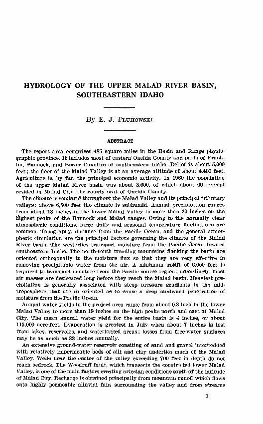
The report area comprises 485 square miles in the Basin and Range physio graphic province. It includes most of eastern' Oneida County and parts of Frank lin, Bannock, and Power Counties of southeastern Idaho. Relief is about 5,000 feet; the floor of the Malad Valley is at an average altitude of about 4,400 feet. Agriculture is, by far, the principal economic activity. In 1960 the population of the upper Malad River basin was about 3,600, of which about 60 percent resided in Malad City, the county seat of Oneida County.
The climate is semiarid throughout the Malad Valley and its principal tributary valleys; above 6,500 feet the climate is subhumid. Annual precipitation ranges from aibout 13 inches in the lower Malad Valley to more than 30 inches on the highest peaks of the Bannock and Malad ranges. Owing to the normally clear atmospheric conditions, large daily and seasonal temperature fluctuations are common. Topography, distance from the Pacific Ocean, and the general atmos pheric circulation are the principal factors governing the climate of the Malad River basin. The westerlies transport moisture from the Pacific Ocean toward southeastern Idaho. The north-south trending mountains flanking the barm are oriented orthogonally to the moisture flux so that they are very effective in removing precipitable water from the air. A minimum uplift of 6,000 feet is required to transport moisture from the Pacific source region; accordingly, most air masses are desiccated long before they reach the Malad basin. Heaviest pre cipitation is generally associated with steep pressure gradients in th^ mid- troposphere that are so oriented as to cause a deep landward penetration of moisture from the Pacific Ocean.
Annual water yields in the project area range from about 0.8 inch in the lower Malad Valley to more than 19 inches on the high peaks north and east of Malad City. The mean annual water yield for the entire basin is 4 inches, or about 115,000 acre-feet. Evaporation is greatest in July when about 7 inches is lost from lakes, reservoirs, and waterlogged areas; losses from free-water surfaces may be as much as 38 inches annually.
An extensive ground-water reservoir consiting of sand and gravel inter^edded with relatively impermeable beds of silt and clay underlies much of the Malad Valley. Wells near the center of the valley exceeding 700 feet in depth do not reach bedrock. The Woodruff fault, which transects the constricted lower Malad Valley, is one of the main factors creating artesian conditions south of the latitude of Malad City. Recharge is obtained principally from mountain runoff which flows onto highly permeable alluvial fans surrounding the valley and from streams
2 HYDROLOGY, UPPER MALAD RIVER BASIN, IDAHO
that flow across the valley floor. On the basis of a \v<a tor-balance analysis, under flow from the project area was estimated to be 28,000 acre-feet annually, surface- water outflow was 51,000 acre-feet, and transbasin imports were about 4,000 acrenfeet.
The principal tributaries of the Malad River are perennial along their upper and middle reaches and have well-sustained low flows. During the growing season, all surface waiter entering the Malad Valley is used for irrigatior. Some irriga tion is practiced in the principal tributary valleys; however, a shortage of suitable reservoir sites has hampered surface-water development in these areas. The highly porous deposits underlying the Malad Valley tend to attenuate flood peaks. An unusual combination of meteorologic events early in 1962 effectively counteracted the high absorptive capacity of the valley and predisposed the basin to high flood risk. Subsequent rapid snowmelt combine 1 with frozen ground produced 'the extraordinary flood of February 12, 1962.
Calcium and bicarbonate commonly are the most abundant ions in the surface waters of the upper Malad River basin. In August 1967, the dissolved-solids content of streamflow ranged from 200 to 350 milligrams per liter in the middle and upper parts of the basin; however, much greater values were measured in the Malad River between Woodruff and Cherry Creek Lane. Witl the exception of that reach, the surface water of the project area is suitable fo*" irrigating all but the most sensitive crops.
The total water yield is not sufficient to meet all the water needs of the basin. A comprehensive water-management plan Is required to ensure optimal use of the water resource.
INTRODUCTION
PURPOSE
The upper Malad River basin is an agricultural region whose econ omy depends largely on irrigation. Although annual precipitation on the valley floor is marginal even in wet years, moderate precipitation on the surrounding highlands yields sufficient runoff to supply much of the basin's water needs. Overland runoff from, tl ^ hard-rock uplands spills onto the permeable valley floor where part of it filters into the ground. Some of the water that seeps into the ground perco lates through the zone of aeration and eventually merges with the ground-water reservoir. Irrigation for the production of high-value cash crops is provided by diverting streams into ditches and by pump ing from the extensive ground-water reservoir underlying the Malad Valley.
Despite the generally favorable situation, the basin i? not without its problems with regard to water. Heavy pumping of artesian aquifers underlying the southern part of the valley has lowered pressures to such an extent that many wells which once flowed freely no longer do so, and the discharge of flowing wells has diminished. The density of water-loving plants has increased in much of the lower part of the valley owing to irrigation from numerous flowing wells. Large tracts south of Malad City are unsuitable for agriculture beer use of heavy
INTRODUCTION 6
concentrations of salt and alkali in the soils especially in areas of ground-water discharge.
The purpose of this report is to evaluate the hydrologic factors that directly or indirectly affect the water balance of the upper Malad River basin. Specifically, an attempt is made to assess the water yield of the basin. Surface-water supplies are evaluated, and methods of increasing the beneficial use of water in the basin are suggested.
LOCATION AND EXTENT OF AREA
The study area comprises the 485-square-inile drainage area of the Malad River above Woodruff, Idaho. It includes most of eastern Oneida County and parts of Franklin, Bannock, and Power Counties of southeastern Idaho (fig. 1). Malad City, the principal town in the basin, is about 50 miles south of Pocatello, Idaho, and about 100 miles north of Salt Lake City, Utah.
The Malad Valley is bounded on the east by the Bannock and the Malad Ranges and on the west and southwest by the Blue Spring Hills (fig. 3). On the north the valley is divided into two principal drainage systems which are separated by a spur of the Bannock Range. South of the spur much of the valley is underlain by an artesian aquifer. The principal axis of the basin trends northward and is about 37 miles in length; the basin is about 24 miles across at its widest point.
PREVIOUS INVESTIGATIONS
One of the earliest accounts of the geology and landforms of the upper Malad River basin was made by Bradley (1873). Peale (1879) described the limestone formations which crop out in the Blue Spring Hills. Several of the principal stratigraphic units of the basin were defined by Piper (1924). The Woodruff fault, which trends eastward across the constricted south end of the Malad Valley, was described in a report by Mower and Nace (1957). That report contains a descrip tion of the geology of the basin in relation to the ground-water reservoir.
Thompson and Faris (1932) measured the discharge from artesian wells south of Malad City in 1931. They made a preliminary evalua tion of the water resources of the basin and recommended that surface supplies be used in the spring and early summer and that ground water be reserved for use during periods of low flow. This suggestion was made to conserve water by improving the efficiency of water use in the basin. Livingston and McDonald (1943) estimated the total flow from artesian wells to be 6,000 gpm (gallons per minute) in the Malad Valley during July 1943. They measured considerable subsur-
367-852 0 70 2

4 HYDROLOGY, UPPER MALAD RIVER BASIN, IDAHO
face migration of water through uncapped or leaky artesian wells. Mower and Nace (1957) estimated evapotranspiration losses from
the middle and lower parts of the Malad Valley to be about 37,000 acre-feet a year. Water-level measurements for some observation wells, records of daily discharge for gaging stations, and discharge measurements made at partial-record sites are published in annual water-supply papers .and open-file reports of the U.S. Geological Survey.
114°45
44
43'
42°
113° 112°
Rupert
MONTANA
IDAHO
St. Anthony I
O
IS i£
CARIBC U
Soda Springs
( __
UTAH50 MILES
FIGUKE 1. Map of southeastern Idaho showing area of investigation.
INTRODUCTION
WELL-NUMBERING SYSTEM
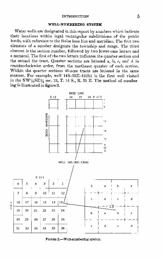
Water wells are designated in this report by numbers which indicate their locations within legal rectangular subdivisions of the public lands, with reference to the Boise base line and meridian. The fir^t two elements of a number designate the township and range. The third element is the section number, followed by two lower-case letters and a numeral. The first of the two letters indicates the quarter section and the second the tract. Quarter sections are lettered a, b, c, and d in counterclockwise order, from the northeast quarter of each section. Within the quarter sections 40-acre tracts are lettered in the same manner. For example, well 14S-35E-13dbl is the first well visited in the NW^SE^ sec. 13, T. 14 S., K. 35 E. The method of number ing is illustrated in figure 2.
R 1 E.
BASE LINE34 35 36 R 37 E
WELL 14S-35E-13dbl
R 35 E
6
7
18
19
30
31
5
8
17
20
29
32
4
9
16
21
28
33
3
10
15
22
27
34
2
11
14
23
26
35
1
12 1
13cL
24
25
36
FIGUBE 2. Well-numbering system.
6 HYDROLOGY, TIPPER MALAD RIVER BASIN, IDAHO
GEOGRAPHY
POPULATION
The Malad Valley was first settled in 1855, but the settlement dis banded in 1858 owing to the destruction of crops by locurts. The first permanent settlement of the Malad Valley was established in 1864 at the site of what is now Malad City (Howell, 1960). In 1866 the Oneida County seat was moved from Soda Springs to Malad City which helped spur the growth of the town. By 1870, Malad City had a pop ulation of 571, and it continued to grow steadily for another 50 years. Owing to a good perennial supply of wrater, wild game, fertile lands, and an adequate supply of timber nearby, the valley was largely settled by the turn of the century. A railroad, built in 1906, stimulated popu lation growth by connecting the expanding agricultural economy of the Malad Valley with the large population centers of Ogden and Salt Lake City, Utah. The population of the basin continued to increase until shortly after World War I.
After the boom years of World War I, the population of the study basin followed the downward trend of many other farm-based econ omies in the Nation. The population of Oneida County, for example, has declined steadily since 1920. By 1960, the countywide population was only 54 percent of the 1920 population as shown in tl °, following table:
Population of Malad City and Oneida County, Idaho
I960 1950 1940 1930 1920 1910 1900
Malad City....................................... 2,274 2,715 2,731 2,535 3,OfO 1,904 1,360Oneida County................................... 3,603 4,387 5,417 5,870 6,723 ................
Malad City, on the other hand, showed substantial growth between 1900 and 1920. After a decline in population during the 1920's some recovery occurred during the 1930's; however, since 1950 its popula tion has declined again. Much of the increase in the population of Malad City during 1900-50 probably resulted from a tendency on the part of farmers to move into town as improved roads and automobiles reduced travel time between town and farm. The countywide decline in population can be ascribed to an exodus of people to large urban centers and a growing tendency toward larger farms. Improved mech anization has greatly increased the acreage which a farmer can success fully cultivate. Efficient farms grow at the expense of less efficient enterprises; thus, the basin has fewer farms today than at any time since 1900.

GEOGRAPHY 7
TOPOGBAPHY AND DBAINAGE
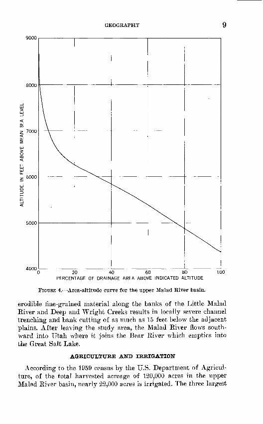
The upper Malad River basin is in the Basin and Range physio graphic province (Fenneman, 1931). Extreme relief is about 5,000 feet. The average altitude of the Malad Valley floor is about 4,400 feet, and it ranges from about 4,350 feet at Woodruff to 4,800 feet where the valley abuts the surrounding highlands. The Malad T7"alley has low relief and is about 7 miles wide and 11 miles long. About 3 miles above Woodruff the valley abruptly narrows to a width c f 2 to 3 miles, and this constricted cross section is maintained southward into Utah. Highest altitudes are 9,285 feet at Oxford Peak and 9,001 feet at Mount Elkhorn. Both peaks are part of the Bannock Range which forms the northern and, with the Malad Range, the eastern boundaries of the study basin (figure 3). In the Blue Spring Hills to the west, the highest peaks are less than 8,000 feet. The mean alti tude of the basin is 5,600 feet (fig 4), and only 6 percent of the r.rea is above 7,000 feet in altitude.
The mountain ranges are oriented north-south, and their crests form the boundaries of the basin everywhere except across the constricted lower Malad Valley. In general, the uplands are well dissected by numerous ephemeral channels which have eroded sharp V-shaped val leys. Both the mountains and their surrounding foothills are being degraded by a combination of sheet wash, gullying, and channel erosion.
The products of the upland erosion have formed alluvial fans at the base of the foothills. Upon flowing onto the alluvial fans the competence of streams to move sediment is quickly reduced. This is due principally to lower gradients and the rapid infiltration of streamflow into the pervious bed material. As a result of the combi nation of discharge loss and sediment deposition, most ephemeral channels lose their identity a short distance beyond the foothills. The slopes of the alluvial fans gradually decrease until they merge with the valley floor.
In general, the principal tributary basins, the Little Malad River and Devil and Deep Creeks, are well dissected and characterized by moderate gradients and narrow flood plains. These streams ore pe rennial north of the Malad Valley and are sustained by springs and transbasin diversions. The flow in all streams that move acrcss the Malad Valley is generally sluggish owing to the predominantly gentle gradients. The Malad River, whose source is a spring on the valley floor north of Pleasantview, flows entirely within the western part of the Malad Valley; consequently its gradient is low and its course is meandering. Bank erosion may be severe during high-flow periods in all stream channels traversing the Malad Valley. Highly

HYDROLOGY, UPPER MALAD RIVER BASIN, IDAHO
EXPLANATION
R 34 EU|« «ft
T. 10 S
42°30' =
T. 11 S
Valley floor Alluvial fansIncludes flood plains of the _____
principal tributary valleys \S\\~-\-\iand alluvial and lacustrine CsVvvlplain,, of the Malad Valley Dissected uplands
Local relief generally less than 1,500 feet
Dissected uplandsLocal relief generally greater
than 1,500 feet
Spring
T 12S
T. 13 S
T. 14 5
T.15S
T. 16 S
. Generalized landforni map of the upper Malad Riv?r basin.
GEOGRAPHY
9000
8000
7000
6000
5000
40000 20 40 60 80
PERCENTAGE OF DRAINAGE AREA ABOVE INDICATED ALTITUDE100
FIGURE 4. Area-altitude curve for the upper Malad River basin.
erodible fine-grained material along the banks of the Little Malad River and Deep and Wright Creeks results in locally severe channel trenching and bank cutting of as much as 15 feet below the adjacent plains. After leaving the study area, the Malad Eiver flows south ward into Utah where it joins the Bear River which empties into the Great Salt Lake.
AGRICULTURE AND IRRIGATION
According to the 1959 census by the U.S. Department of Agricul ture, of the total harvested acreage of 120,000 acres in the upper Malad River basin, nearly 22,000 acres is irrigated. The three largest

10 HYDROLOGY, UPPER MALAD RIVER BASIN, IDAHO
cash crops are winter wheat (1,280,000 bushels), barley (872,000 bushels), and spring wheat (186,000 bushels); potatoes and sugar beets are the principal irrigated row crops. In addition, extensive tracts are devoted to the production of hay and forage crops, partic ularly in the Malad Valley. A substantial part of total farm income is obtained from the sale of cattle and sheep.
Agricultural development in the Malad Valley was b°gun in the mid-1860's. Within a short time nearly the entire flow of streams in the valley was being diverted for irrigation during the growing season. Desirable lands adjacent to the streams were quickly brought under irrigation and further expansion of irrigated r<?reage was slow. Following the appropriation of most surface-water supplies, dry-land farming of wheat and barley was attempted successfully on the foothills surrounding the Malad Valley and in its principal tributary valleys. About 1900 the large potential yield of the artesian basin in the southern part of the valley was recognized. Flowing wells were drilled in a wide area south of Malad City and much new land was brought under irrigation. Development of nonartesian water with pumped wells was begun about 1930, and substantial areas of land north and west of Malad City are irrigated with water from pumped wells. To augment surface-water supplies, a large part of the headwater flow of Birch Creek in the Snake River basin was diverted into Devil Creek. This imported water is the principal supply for much of the irrigated land in Devil Creek valley and the part of the Malad Valley lying north of Malad City. Small storage reservoirs have been constructed on Deep Creek, Davis Creek, and the Little Malad River. Currently (1967) a new reservoir is being constructed on the Little Malad River near Daniels, about 3i/£ miles above Elkhorn Dam.
Surface-water users in the Malad Valley recognized early the need for careful management of the comparatively small quantity of water that is available to them. They are, moreover, aware tha.t much im provement in surface-water management is possible by employing more efficient engineering and land-use practices. In contrast to the coopera tive efforts with regard to surface water, development and use of ground water has been uncoordinated and without much regard to the overall water economy of the valley. Waste of ground water, especially from flowing wells, commonly occurs with little action taken by well owners to limit waste. Widespread declines of piezometric levels in the artesian aquifers may, in part, be traced to the haphazard and inef ficient use of the valley's ground-water resources. Owing to excessive application and waste of water on some tracts of land, other tracts of arable land remain unirrigated because water is not available. Clearly,
CLIMATE 11
optimum use of the water resources of the basin cannot be attained until both surface-water and ground-water supplies are efficiently utilized.
VEGETATION
Water-loving vegetation of generally low economic value is domi nant in low-lying parts of the Malad Valley. Phreatic vegetation also grows along the banks of many streams, where it serves to maintain channel stability. According to Mower and Nace (1957), the pre vailing type of phreatophyte is mainly a function of the depth to \vater. In general alfalfa (an important cash crop) and rabbitbrush grow where the depth to water ranges from 10 to 35 feet; desert saltsrass, greasewood, and pickleweed grow where the depth to water is £ to 10 feet; sedge, wire rush, marsh reedgrass, and desert saltgrass grow where the depth to water is 1 to 5 feet; rushes, cattails, and sedges grow where depth to water is only a few inches, or where water is ponded during most of the growing season. In all, water-loving vegeta tion occupies nearly 13,000 acres of bottom land, principally south of Malad City.
In uncultivated valley areas where the depth to water is beyond the reach of water-loving vegetation, sagebrush and native grasses rre the most abundant plants. Sagebrush is the dominant plant form on the foothills between altitudes of 5,600 and 6,000 feet where it is usually associated with juniper. Juniper, scrub oak, and scrub maple arc prev alent from 6,000 to 7,000 feet. Above 7,000 feet, dense stands of pine, fir, spruce, and aspen grow wherever the environment is favorable.
CLIMATE
PRIMARY CONTROLS
The climatic regimen of the upper Malad River basin is governed by the same physical elements that control daily weather throughout the temperate zone. Differential heating between landmasses and the oceans results in the establishment of the semipermanent atmospheric centers of high and low pressure. In winter, the extensive land areas of the northern hemisphere lose heat to the atmosphere at a faster rate than the adjacent oceans. The consequent buildup of cold air over the continent creates reservoirs of heavy dense air at the surface. The relatively warmer and therefore lighter air over the oceans tends to rise, generating centers of low pressure. This process reverses itself in summer when landmasses are warmer than ocean areas at the same latitude.
The principal centers of weather action affecting the climate of the Malad basin in winter are the Aleutian low and the Great Basin high;
367-858 O 70 <3
12 HYDROLOGY, UPPER MALAD RIVER BASIN, IDAHO
in summer the eastern Pacific high is dominant. Each of th°.se pressure cells is characterized by seasonal changes in intensity; in addition, the Aleutian low and the eastern Pacific high migrate considerably. Sea sonal variations in the characteristics of large quasi-permanent pres sure systems stem from the changing pattern of land and sea tempera tures previously outlined. The Aleutian low and the Great Basin high are most intense in winter, whereas the eastern Pacific high, is weakest at that time. With the approach of summer the Great Basin high dissipates and the Aleutian low weakens considerably. The eastern Pacific high, on the other hand, attains its peak intensity in summer and dominates the weather of a large part of the West, including south eastern Idaho.
Seasonal variation of air pressure at the surface and global atmos pheric movement strongly influence the climate of the Malad River basin. Weather systems are transported from west to east by the pre vailing westerlies which are the principal element of the general cir culation pattern affecting the climate of southeastern Idaho. Although mostly well above the friction zone near the earth's surface, the west erlies vary widely in direction and intensity from day to day. Much of this variation is due to planetary or long waves in the up ^er wester lies that are now generally recognized as the primary factor controlling weather in the middle latitudes. It has also been shown that wave trains in the upper air circulation are closely related to the semiper manent pressure centers at sea level (Klein, 1956, p. 203-219). There fore, the orientation of the planetary waves with respect to the Malad Valley plus large-scale centers of weather action at the surface consti tute the principal atmospheric controls on weather and climate in the study basin.
The Pacific Ocean is the primary source of moisture for much of the West owing to the prevailing west-to-east atmospheric circulation. Ac cordingly, the topographic barriers between the upper Malad River basin and the Pacific Ocean have a profound effect on the amount of moisture reaching the basin. Because the numerous north-south moun tain ranges are oriented orthogonally to the moisture flow from the Pacific Ocean, they may be labeled as "moisture barriers." The amount of uplift to which a given quantity of air is subjected depends on the specific route it is forced to take over the mountains. However, it has been shown that Pacific airmasses are uplifted at least 6,000 feet by the time they arrive over the Malad River basin (U.S. Department of Commerce, 1953, p. 11). Because most of the moisture in the atmos phere is concentrated within 6,000 feet of the surface, much of the precipitable water of any maritime airmass will be removed long before it reaches the Malad River basin.
CLIMATE 13
10
PRECIPITATION, IN INCHES
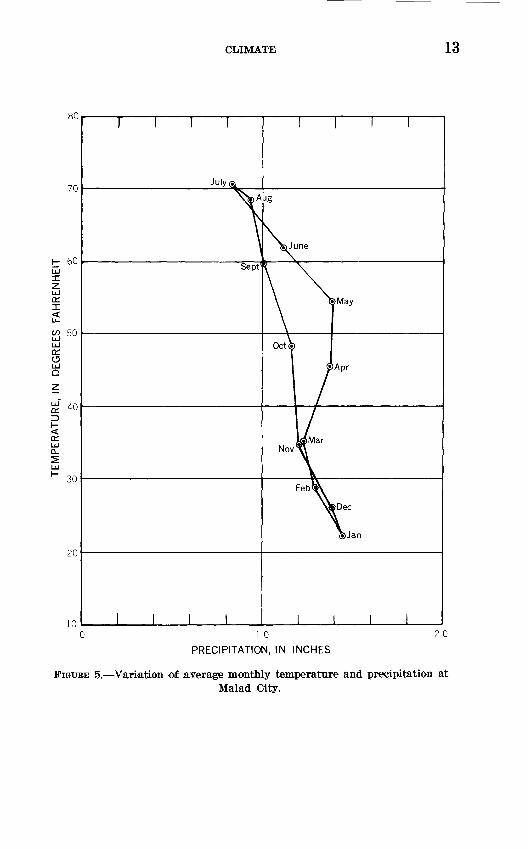
FIGURE 5. Variation of average monthly temperature and precipitation atMalad City.
14 HYDROLOGY, UPPER MALAD RIVER BASIN, IDAHO
TEMPERATURE
SEASONAL VARIATION'S
Temperatures in the upper Malad River basin have strong conti nental characteristics as demonstrated by the graph depicting the variation of average monthly temperature and precipitation for Malad City (fig. 5). The range of mean monthly temperatures at Malad City is almost 50 °F.; extreme temperatures range from 25° to 108 °F. Temperatures as low as 33°F have been recorded at the Malad City Airport. January is the coldest month and July the warmest. Decem ber is normally colder than February, which is characteristic of a continental-type climate.
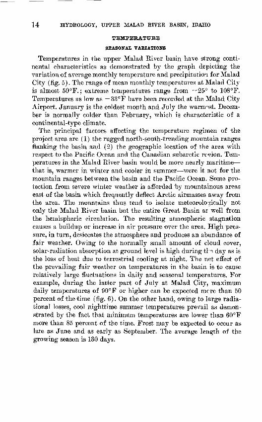
The principal factors affecting the temperature regimen of the project area are (1) the rugged north-south-trending mountain ranges flanking the basin and (2) the geographic location of the area with respect to the Pacific Ocean and the Canadian subarctic region. Tem peratures in the Malad River basin would be more nearly maritime that is, warmer in winter and cooler in summer were it not for the mountain ranges between the basin and the Pacific Ocean. Some pro tection from severe winter weather is afforded by mountainous areas east of the basin which frequently deflect Arctic airmasses away from the area. The mountains thus tend to isolate meteorologically not only the Malad River basin but the entire Great Basin a? well from the hemispheric circulation. The resulting atmospheric stagnation causes a buildup or increase in air pressure over the area. High pres sure, in turn, desiccates the atmosphere and produces an abundance of fair weather. Owing to the normally small amount of cloud cover, solar-radiation absorption at ground level is high during tH day as is the loss of heat due to terrestrial cooling at night. The net effect of the prevailing fair weather on temperatures in the basin is to cause relatively large fluctuations in daily and seasonal temperatures. For example, during the latter part of July at Malad City, maximum daily temperatures of 90°F or higher can be expected mrre than 50 percent of the time (fig. 6). On the other hand, owing to large radia- tional losses, cool nighttime summer temperatures prevail as demon strated by the fact that minimum temperatures are lower than 60 °F more than 85 percent of the time. Frost may be expected to occur as late as June and as early as September. The average length of the growing season is 130 days.
PERCENTAGE OF TIME MINIMUM DAILY
TEMPERATURE EQUALED OR WAS
LOWER THAN THAT SHOWN
§m -F* w ro oooo
\
PERCENTAGE OF TIME MAXIMUM DAILY
TEMPERATURE EQUALED OREXCEEDED THAT SHOWN
16 HYDROLOGY, TIPPER MALAD RIVER BASIN, IDAHO
VERTICAL TEMPERATURE GRADIENT
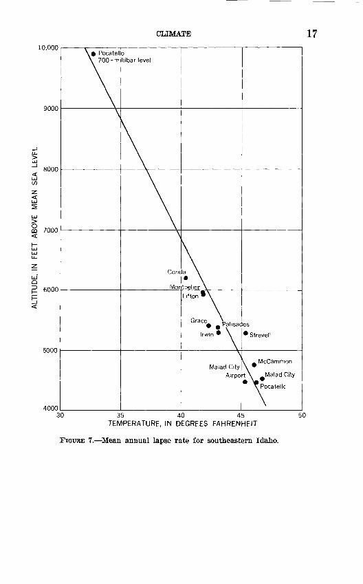
Evapotranspiration, one of the principal elements in any water- budget analysis, is highly temperature dependent. For evaluation of this important variable, some knowledge regarding the rate of change of temperature with altitude (lapse rate) is often helpful. An accurate assessment of the regional lapse rate was needed to estimate mean annual temperature, which was then used to compute wpter loss by evapotranspiration throughout the basin. Owing to the scanty meteorologic data in the upper Malad River basin, it was necessary to use climatic data for all of southeastern Idaho in the lapse-rate analysis.
The lapse rate over southeastern Idaho varies seasonally; it is greater in summer than in winter. In summer, a high rate of absorbed radiation at the surface during the day causes substantial warming of the air immediately above the ground. The effect of this hept exchange on ambient temperature decreases progressively with incr3asing alti tude so that air temperatures near the surface are higher relative to those in the midtroposphere and upper troposphere. In winter, on the other hand, large outgoing radiational losses at the surface produce sharp temperature inversions at night. Accordingly, nighttime tem peratures in the valley may be much lower than those observed in the mountains. The overall effect is to reduce the average lapse rate in winter to about 1°F per 1,000 feet from the maximum seasonal rate in summer of about 3.5°F per 1,000 feet.
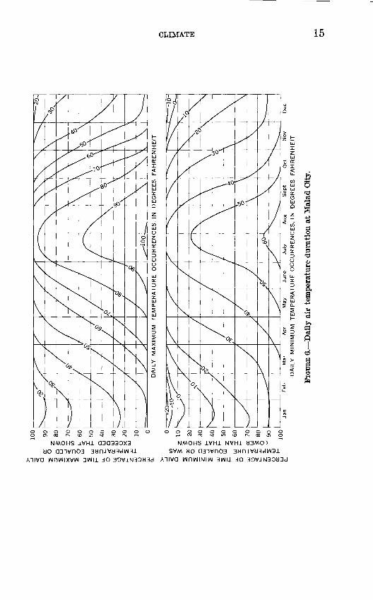
The mean annual lapse rate in the basin is about 2.5°F per 1,000 feet, as shown in figure 7, which is based on long-term records of U.S. Weather Bureau stations. The lapse rate obtained from figure 7 is just 0.2 C F lower than that of the standard atmosphere (Landsberg, 1958, p.161).
CLIMATE 17
10,000
Malad CityAirport \ Malad City
» ^Pocatellc
400035 40 45
TEMPERATURE, IN DEGREES FAHRENHEIT
FIGURE 7. Mean annual lapse rate for southeastern Idaho.

18 HYDROLOGY, UPPER MALAD RIVER BASIN, IDAHO
HYDROMETEOROLOGY
With the exception of a relatively small amount of surface water imported from the Birch Creek basin, virtually all the v^ater in the study area is obtained from precipitation. Clearly, any assessment of the water potential of the basin must be predicated on a thorough analysis of all aspects of precipitation. To accomplish this task, one should analyze the causes of rainfall if an insight is to be gained into the nature of this critical component of the hydrologic environment.
CIRCULATION PATTERNS FAVORING ABOVE-NOLJCAL PRECIPITATION
The amount of moisture available for precipitation over the Malad Valley is dependent on the strength of the westerlies over the area. The strength of the westerlies, in turn, is a function of the pressure gradient within the troposphere. Any orientation of pressure patterns that causes a strong movement of air from the Pacific Cbean (espe cially the southeastern Pacific) toward Idaho is likely to produce heavy precipitation.
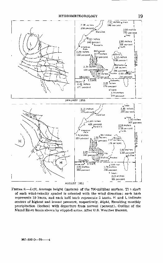
The upper air regime commonly associated with heavy precipitation in Idaho is characterized by a trough of low pressure off the California coast with a stronger-than-normal ridge oriented north-south over the Rocky Mountains. The southwesterly movement of air associated with such a system can move vast quantities of moisture-laden air from the southeast Pacific Ocean area inland toward southeastern Idaho. For example, in January 1956 a deep trough of low pressure off the west coast of North America (fig. 8) produced a steep pressure gradient in the eastern Pacific Ocean; concomitantly, a ridge of high pressure developed along the Rocky Mountains. This pressure field induced a stronger-than-normal flow of air to move over the project area from the Pacific Ocean. Moreover, the trajectory of this air was from the west-southwest so that much of its path was over warm ocean surfaces. The high moisture content of the maritime air, in combination with the strong flow pattern, resulted in above-normal precipitation in much of the West. Mean monthly precipitation in areas adjacent to the upper Malad River basin was above normal, ranging from 128 to 260 percent of normal, as shown in the upper right-hand part of figure 8. Wave patterns in the upper westerlies are most sinuous in the late fall and winter; in summer th°,y are less pronounced. The overall effect of the weakened wave pattern in sum mer is to reduce the ability of moisture-laden airmasses tc penetrate very far inland, thereby fostering aridity in much of the West.
Despite weakening of the atmospheric circulation over southeastern Idaho in summer, the influx of moisture from the southeastern Pacific
HYDROMETEOROLOGY
2.29 inches McCammon 164 percent^ 3_Zl' nches
' \ 260 percent/:::: ..4
2.35 inches"::
165 percent^
j:::: 2.44 inches^
__IDAHO ^U74~percent* _ _
Snowville UTAH
2.26 inches
171 percent
Grace1 53 inches
[128 percent
[ontpeHer(. '1.86 inches
J 186 percent Veston O93lriSrl
155 percentI -r
3.25 inches \ 1 179 percent Vy
Logan 2.74 inches
177 percent
M
JANUARY 1956
3.39 inches
390 percent)
. Gray I?.32 inches
307 percent2.58 inches i
2.53 percent .
0.82 inches
255 percent (v jtJl±""-"" -^ iirace\ ::V.V107 percent ill inches '
.ii{|:::?| 178 P ercent
) £^^y inc ii'Malad"City l.uy percent 242 percent!1.:::-:;/ ^ ,-^Lifton 1
';:;:,1.23 inches^Preston r*\ |
IDAJHO ^ 246~percent _ _ ___/ /_ __I
,wvale« UTAH ~ .RichmoTTT") ~1 .95 inches 1.74 inches \ ( I1.95 inches
394 percent
1.74 inches \ )
238 percent Vj Logan
2.25 inches
331 percent
AUGUST 1951
FIGURE 8. Left, Average height (meters) of the 700-millibar surface. Tl * shaft of each wind-velocity symbol is oriented with the wind direction; each barb represents 10 knots, and each half barb represents 5 knots. H and L indicate centers of highest and lowest pressure, respectively. Right, Resulting monthly precipitation (inches) with departure from normal (percent). Outline of the Malad River basin shown by stippled areas. After U.S. Weather Bureau.
367_852 0 7C
20 HYDROLOGY, UPPER MALAD RIVER BASIN, IDAHO
Ocean and, to a lesser extent, from the Gulf of Mexico may occasionally result in heavy rainfall. During the warm season a weak upper air trough in the midtroposphere normally separates the eastern Pacific high from a quasi-stationary high over the South-Central United States. Frontal activity is rarely associated with the trough, and its intensity is so slight that little movement of air is generated by the weak pressure field. Accordingly, high pressure predominates, causing fair weather throughout much of the West. However, if the trough deepens and moves eastward toward the west coast of the United States, a flow of moist air may spread as far as southeast Idaho, and sporadic thunderstorm and shower activity is likely to be generated in the study area.
The mean pressure field for August 1951 shown in the lower part of figure 8 portrays a pattern that is conducive to heavy summer rainfall in southeastern Idaho. The deeper-than-normal trough extending from Washington southwestward to the Pacific Ocean caused a sub stantial flow of moist air to move inland. The anomalous pmoimts of atmospheric moisture over southeastern Idaho produced rainfall which ranged from 107 to 426 percent of normal for the month, 'as shown in the lower right-hand part of figure 8.
PEESISTENX3E OF CIECULATION PATTEENS
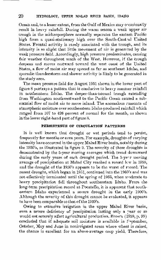
It is well known that drought or wet periods tend to persist, frequently for months or even years. For example, droughts of varying intensity have occurred in the upper Malad River basin, notably during the 1930's, as illustrated in figure 9. The severity of these droughts is demonstrated by the 5-year moving averages which trend downward during the early years of each drought period. The 5-ye^r moving average of precipitation at Malad City reached a record lew in 1958, and the drought of the 1950's appears to be the worst of record. The recent drought, which began in 1951, continued into the 1960's and was not effectively terminated until the spring of 1963, when iroderate to heavy precipitation fell throughout southeastern Idaho. From the long-term precipitation record at Pocatello, it is apparent that south eastern Idaho experienced a severe drought in the early 1900's. Although the severity of this drought cannot be evaluated, it appears to have been comparable to that of the 1930's.
Owing to extensive irrigation in the upper Malad River basin, even a severe deficiency of precipitation lasting only a ^ear or so would not severely affect agricultural production. Brown (1959, p. 99) concluded that if adequate soil moisture is available in J? Q/ptember, October, May and June in nonirrigated areas where wheat is raised, the chance is excellent for an above-average crop yield. Therefore,
22 HYDROLOGY, UPPER MALAD RIVER BASEST, IDAHO
during a severe drought, it may be possible to have at least an average crop yield even in dry-farm areas provided that rainfall is well timed. During a protracted dry spell, however, the surface-water supplies may become seriously reduced after carryover water from earlier wet periods is depleted. Moreover, increased pumping of ground-water reserves to counter the effect of drought on crops, in combination with sharply lowered recharge, may cause substantial decline? in water levels.
COLD-SEASON DROUGHT
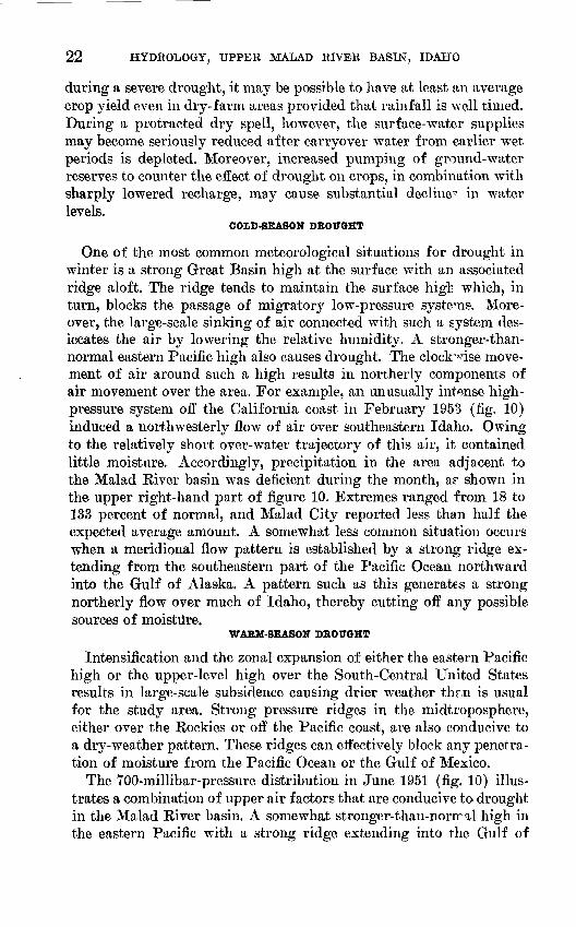
One of the most common meteorological situations for drought in winter is a strong Great Basin high at the surface with an associated ridge aloft. The ridge tends to maintain the surface high which, in turn, blocks the passage of migratory low-pressure systems. More over, the large-scale sinking of air connected with such a system des iccates the air by lowering the relative humidity. A stronger-than- normal eastern Pacific high also causes drought. The clockwise move ment of air around such a high results in northerly components of air movement over the area. For example, an unusually intense high- pressure system off the California coast in February 1953 (fig. 10) induced a northwesterly flow of air over southeastern Idaho. Owing to the relatively short over-water trajectory of this air, it contained little moisture. Accordingly, precipitation in the area adjacent to the Malad River basin was deficient during the month, a^ shown in the upper right-hand part of figure 10. Extremes ranged from 18 to 133 percent of normal, and Malad City reported less than half the expected average amount. A somewhat less common situation occurs when a meridional flow pattern is established by a strong ridge ex tending from the southeastern part of the Pacific Ocean northward into the Gulf of Alaska. A pattern such as this generates a strong northerly flow over much of Idaho, thereby cutting off any possible sources of moistilre.
WARM-SEASON DROUGHT
Intensification and the zonal expansion of either the eastern Pacific high or the upper-level high over the South-Central United States results in large-scale subsidence causing drier weather thr,n is usual for the study area. Strong pressure ridges in the midtroposphere, either over the Rockies or off the Pacific coast, are also conducive to a dry-weather pattern. These ridges can effectively block any penetra tion of moisture from the Pacific Ocean or the Gulf of Mexico.
The YOO-millibar-pressure distribution in June 1951 (fig. 10) illus trates a combination of upper air factors that are conducive to drought in the Malad River basin. A somewhat stronger-than-norrral high in the eastern Pacific with a strong ridge extending into the Gulf of
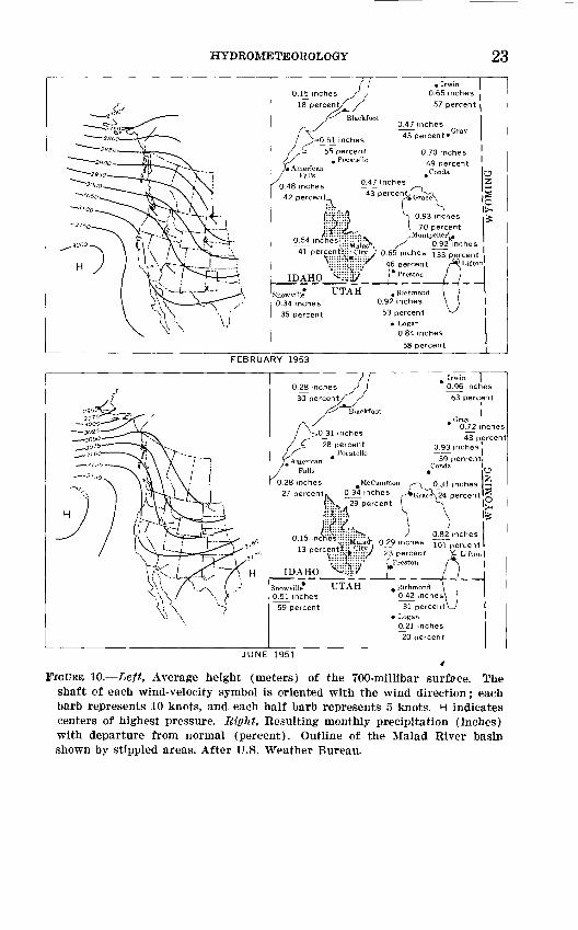
HYDROMETEOROLOGY 23
. , __ . r^?.?.%City / rj.65 inches 133 percent
^i-liiniiii:;^ 46 percent r^Lifton
FEBRUARY 1953
0.28 inches
30 percent
0.96 inches
63 percent I
* 0-72 inches
43 percent 0.93 inches!
0.82 inches inches To~fpercen t
Lifton
AHO _ OW_ __ £_ _ _DAHOSnowville- 0.51 inches
59 percent
UTAH
i
1
JUNE 1951t
FIGURE 10. Left, Average height (meters) of the 700-millibar surface. The shaft of each wind-velocity symbol is oriented with the wind direction; each barb represents 10 knots, and each half barb represents 5 knots. H indicates centers of highest pressure. Right, Resulting monthly precipitation (inches) with departure from normal (percent). Outline of the Malad River basin shown by stippled areas. After U.S. Weather Bureau.
24 HYDROLOGY, UPPER MALAD RIVER BASEST, IDAHO
Alaska effectively shielded much of Idaho from landward movement of moist Pacific airmasses. Moreover, the subsidence resulting from the high-pressure cell produced cloudless skies for extended periods dur ing the month. Despite above-normal sunshine, temperatures were below expected seasonal levels owing to the influx of cool air from the Gulf of Alaska.
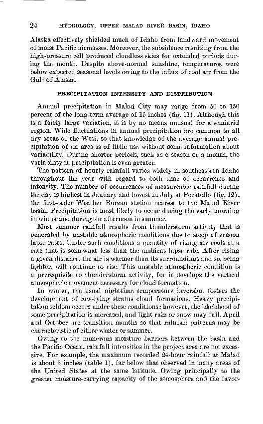
PRECIPITATION INTENSITY AND DISTRIBUTION
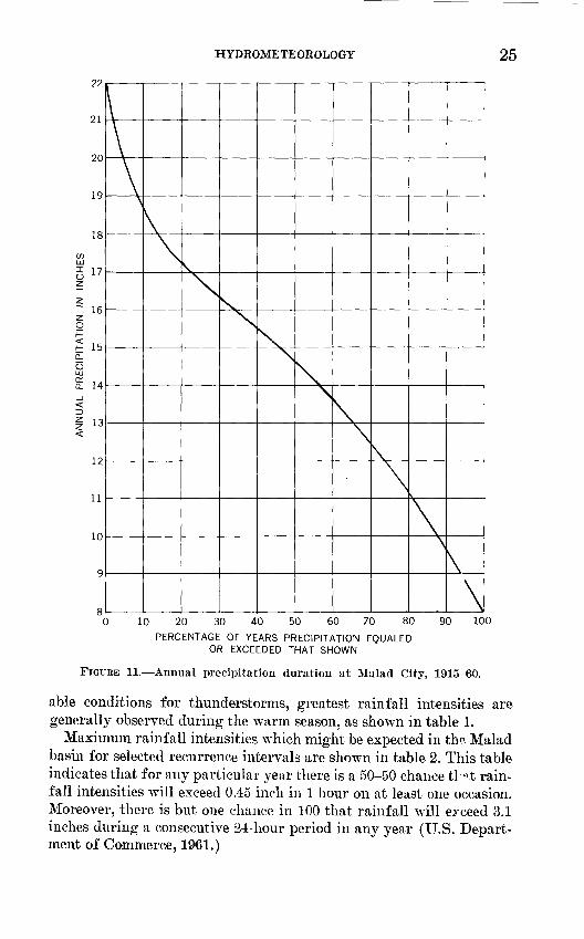
Annual precipitation in Malad City may range from 50 to 150 percent of the long-term average of 15 inches (fig. 11). Although this is a fairly large variation, it is by no means unusual for a semiarid region. Wide fluctuations in annual precipitation are common to all dry areas of the West, so that knowledge of the average annual pre cipitation of an area is of little use without some information about variability. During shorter periods, such as a season or a month, the variability in precipitation is even greater.
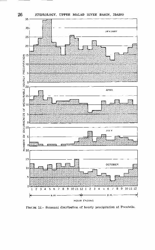
The pattern of hourly rainfall varies widely in southeastern Idaho throughout the year with regard to both time of occurrence and intensity. The number of occurrences of measureable rainfall during the day is highest in January and lowest in July at Pocatello (fig. 12), the first-order Weather Bureau station nearest to the Malad River basin. Precipitation is most likely to occur during the early morning in winter and during the afternoon in summer.
Most summer rainfall results from thunderstorm activity that is generated by unstable atmospheric conditions due to steep afternoon lapse rates. Under such conditions a quantity of rising air cools at a rate that is somewhat less than the ambient lapse rate. After rising a given distance, the air is warmer than its surroundings and so, being lighter, will continue to rise. This unstable atmospheric condition is a prerequisite to thunderstorm activity, for it develops tH vertical atmospheric movement necessary for cloud formation.
In winter, the usual nighttime temperature inversion fosters the development of low-lying stratus cloud formations. Heavy precipi tation seldom occurs under these conditions; however, the likelihood of some precipitation is increased, and light rain or snow may fall. April and October are transition months so that rainfall patterns may be characteristic of either winter or summer.
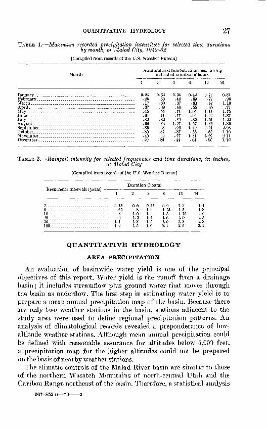
Owing to the numerous moisture barriers between the basin and the Pacific Ocean, rainfall intensities in the project area are not exces sive. For example, the maximum recorded 24-hour rainfall at Malad is about 3 inches (table 1), far below that observed in many areas of the United States at the same latitude. Owing principally to the greater moisture-carrying capacity of the atmosphere and the favor-
HYDROMETEOROLOGY 25
22
21
20
19
17
~ 16
15
14
13
12
11
10
\
30 40 50 60 70 8010 20PERCENTAGE OF YEARS PRECIPITATION EQUALED
OR EXCEEDED THAT SHOWN
90 100
FIGURE 11. Annual precipitation duration at Malad City, 1915-60.
able conditions for thunderstorms, greatest rainfall intensities are generally observed during the warm season, as shown in table 1.
Maximum rainfall intensities which might be expected in the Malad basin for selected recurrence intervals are shown in table 2. This table indicates that for any particular year there is a 50-50 chance tH.t rain fall intensities will exceed 0.45 inch in 1 hour on at least one occasion. Moreover, there is but one chance in 100 that rainfall will exceed 3.1 inches during a consecutive 24-hour period in any year (U.S. Depart ment of Commerce, 1961.)
26 HYDROLOGY, UPPER MALAD RIVER BASIN, IDAHO
35
I 20
123456789 10 11 12 1234 56789 10 11 12
HOUR ENDING
FIGURE 12. Seasonal distribution of hourly precipitation at Pocatello.
QUANTITATIVE HYDROLOGY 27
TABLE 1. Maximum recorded precipitation intensities for selected time durations by month, at Malad City, 1940-62
[Compiled from records of the U.S. Weather Bureau]
Accumulated rainfall, in inches, during Month indicated number of hours
12 24
January ............................February. ..........................March--.-....---.-...--....-.--....April...-...----.-...---....-......May. ...............................June.-----.--....--.---...-..---....July................................August--.--.---.----.--.--.-...-.-.September. .........................October _ .........................November ..........................December ..........................
....------..-.--.-.-.-- 0.24
......---...-----.---.- .25
........--...--.--...-- .17-..--..-....--.---..-.- .37....................... .45.........-....----...-- .64........--....-.--..-.- .82....................... .65....................... .35....................... .30....................... .40....................... .20
0.32.30.30.39.54.71.82.86.68.37.62.34
0.34.40.37.40.71.77.82
1.27.96.37.77.44
0.42.69.60.55
1.04.94.82
1.271.49.55
1.31.64
0.7f.7f.8?.65
1.441.221.011.352.01.80
i.69.8C
0.81.96
1.10.71
1.751.371.221.352.981.162 111.16
TABLE 2. Rainfall intensity for selected frequencies and time durations, in inches,at Malad City
[Compiled from records of the U.S. Weather Bureau]
Duration (hours) Recurrence intervals (years)
6 12 24
9
10
SO.......--.-....-..100 .
.......... . 0.45
.............. .65
._ . .8
....... .9
.. .... 1.1
.............. 1.2
0.6.8
1.01.21.31.5
0.751.01.21.41.51.6
0.91.251.51.61.92.1
1.21.51.752.02.32.5
1.41.82.02.52.83.1
QUANTITATIVE HYDROLOGY
AREA PRECIPITATION
An evaluation of basinwide water yield is one of the principal objectives of this report. Water yield is the runoff from a drainage basin; it includes streamflow plus ground water that moves through the basin as underflow. The first step in estimating water yield is to prepare a mean annual precipitation map of the basin. Because there are only two weather stations in the basin, stations adjacent to the study area were used to define regional precipitation patterns. An analysis of climatological records revealed a preponderance of low- altitude weather stations. Although mean annual precipitation could be defined with reasonable assurance for altitudes below 5,000 feet, a precipitation map for the higher altitudes could not be prepared on the basis of nearby weather stations.
The climatic controls of the Malad River basin are similar to those of the northern Wasatch Mountains of north-central Utah and the Caribou Range northeast of the basin. Therefore, a statistical analysis
367-852 O 70 5
28 HYDROLOGY, UPPER MALAD RIVER BASIN, IDAHO
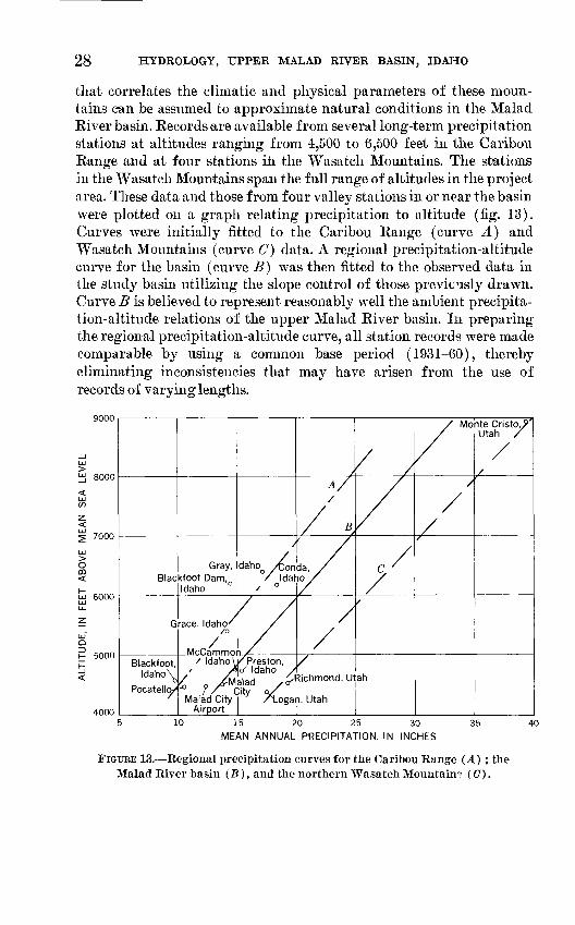
that correlates the climatic and physical parameters of these moun tains can be assumed to approximate natural conditions in the Malad River basin. Records are available from several long-term precipitation stations at altitudes ranging from 4,500 to 6,500 feet in the Caribou Range and at four stations in the Wasatch Mountains. The stations in the Wasatch Mountains span the full range of altitudes in the project area. These data and those from four valley stations in or near the basin were plotted on a graph relating precipitation to altitude (fig. 13). Curves were initially fitted to the Caribou Range (curve A) and Wasatch Mountains (curve C) data. A regional precipitation-altitude curve for the basin (curve B] was then fitted to the observed data in the study basin utilizing the slope control of those previously drawn. Curve B is believed to represent reasonably well the ambient precipita tion-altitude relations of the upper Malad River basin. In preparing the regional precipitation-altitude curve, all station records were made comparable by using a common base period (1931-60), thereby eliminating inconsistencies that may have arisen from the use of records of varying lengths.
9000
8000
7000
6000
5000
4000
Blac
G
Blackfoot, Idaho^
Pocatello/
Gray, (foot Dam, o Idaho
ace, Idaho'/o
/ Idahol
'' rAMalad City
Airport
daho /Con / Idah
¥_/Preston, </ Idaho / alad /a''-ity °/
/^Loga
/
Ja, / 10/
/
Richmond, U1
i, Utah
/
[/
/
ah
/ Mo
/
nte Cristo,J>' Utah /
5 10 15 20 25 30 35 4
MEAN ANNUAL PRECIPITATION, IN INCHES
FIGURE 13. Regional precipitation curves for the Caribou Range (A) ; the Malad River basin (B), and the northern Wasatch Mountain? (C).
QUANTITATIVE HYDROLOGY 29
R 34 E
T 105EXPLANATION
T 11 S
T 12 S
T 135
T 14 S
T 155
T. 165
Line of equal mean annual precipitationInterval 2 and 5 inthes
XFORD PEAK
UTAH
5 MILES
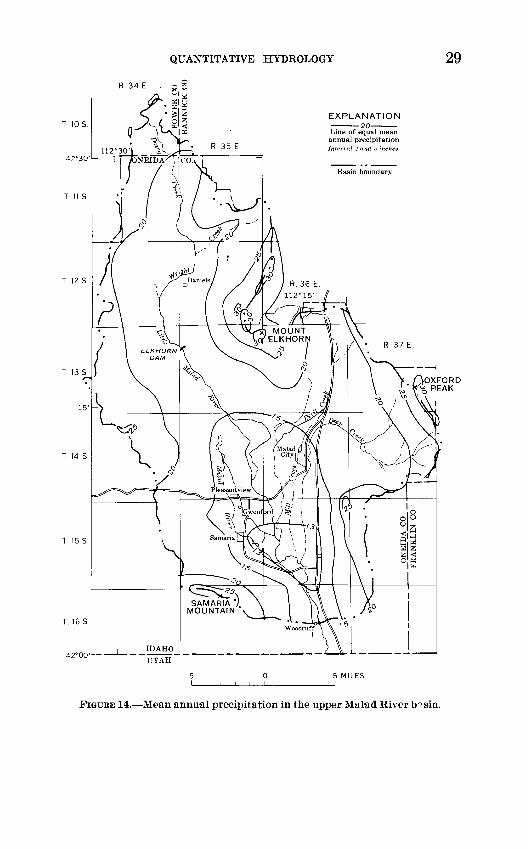
FIGUEE 14. Mean annual precipitation in the upper Malad River bisin.
30 HYDROLOGY, UPPER MALAD RIVER BASIN, IDAHO
With the aid of the regional basin curve (curve B, fig. 13), a mean annual precipitation map (fig. 14) was made for the project area. This figure was prepared by use of an overlay on a topographic map of the basin. The altitudes corresponding to selected amounts of pre cipitation were obtained from the regional basin curve, and their smoothed outline was drawn on the overlay sheet.
The range of mean annual precipitation in the basin is about 20 inches. Precipitation on the highest summits of the basin (about 9,000 feet) is about 21/2 times greater than that on the Malad Piver flood plain above Woodruff. The estimated mean annual precipitation for the entire basin is 18.5 inches.
EVAPORATION
The quantity of water evaporated from free-water surfaces in the project area may be estimated from land-pan evaporation data at nearby stations. The evaporation from free-water surfaces also may be applied to waterlogged land surfaces in the basin to estimate the annual water losses from such areas.
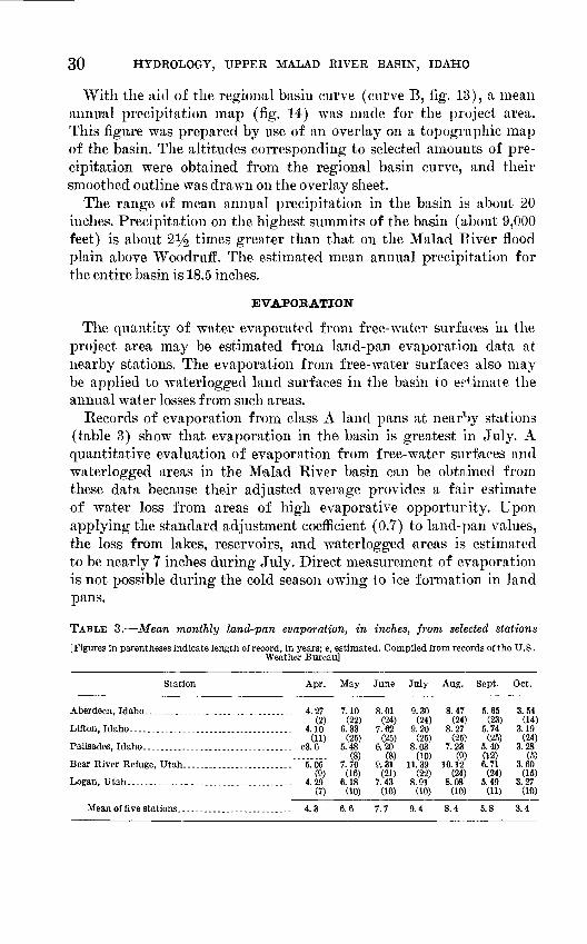
Records of evaporation from class A land pans at nearby stations (table 3) show that evaporation in the basin is greatest in July. A quantitative evaluation of evaporation from free-water surfaces and waterlogged areas in the Malad River basin can be obtained from these data because their adjusted average provides a fair estimate of water loss from areas of high evaporative opporturity. Upon applying the standard adjustment coefficient (0.7) to land-pan values, the loss from lakes, reservoirs, and waterlogged areas is estimated to be nearly 7 inches during July. Direct measurement of evaporation is not possible during the cold season owing to ice formation in land pans.
TABLE 3. Mean monthly land-pan evaporation, in inches, from selected stations
[Figures in parentheses indicate length of record, in years; e, estimated. Compiled from records of the U.S.Weather Bureau]
Station Apr. May June July Aug. Sept. Oct.
Aberdeen, Idaho. ...............
Lifton, Idaho.................. _ .....
Palisades, Idaho....... ...... . . ....
Bear River Refuge, Utah..............
Logan, Utah..... __ ...... _ .......
Mean of five stations... _ .........
............ 4.27(2)
............ 4.10(11)
............ e3.6
............ 5.05(9)
............ 4.29(7)
............ 4.3
7.10(22)
6.33(25)
5.48(8)
7.70(16)
6.18(10)
6.6
8.01(24)
7.62(25)
6.20(8)
9.31(21)
7.43(10)
7.7
9.30(24)
9.20(25)
8.03(10)
11.39(22)
8.91(10)
9.4
8.47(24>
8.27(25)
7.23(9)
10.12(24)
8.08(10)
8.4
5.65(23)
5.74(25)
5.40(12)6.71
(24) 5.49
(11)
5.8
3.54(14)
3.19(24)
3.28(5)
3.60(15)
3.27(10)
3.4
QUANTITATIVE HYDROLOGY 31
To estimate the loss from November through March, use was made of a formula developed by Meyer (1944, p. 238) as follows:
where£T =mean monthly evaporation, in incheses = saturation vapor pressure of water corresponding to
mean monthly temperature, in indies ea = actual air vapor pressure for the month, in inches
/y = mean monthly wind velocity, in miles per hour
From this equation the following values for evaporation, in inches, were obtained : November, 2.3 ; December, 1.1 ; January, 0.9 ; February, 1.1, and March, 2.4. Mean annual land-pan evaporation in the Malad Valley is computed to be 53.4 inches. Applying a 0.7 adjustment co efficient to land-pan values, the computed average annual evaporation from lakes and waterlogged areas is about 38 inches.
EVAPOTBANSPIBATION
Evapotranspiration is water that is returned to the atmosphere from a land area by direct evaporation from water surfaces and moist soil and through transpiration by vegetation. Evapotranspiration has first call on precipitation; it reduces the amount of water avail able for streamflow or for recharge to the ground-water reservoir. It may be considered "nature's take," or that part of precipitation that is consumed by plants, economic or not, and otherwise lost di rectly back to the atmosphere. The rate of evapotranspiration depends chiefly upon air and water temperatures, wind movement, solar radi ation, humidity, availability of moisture, and character of the land surface and plant cover. Many of the climatic parameters a Meeting evapotranspiration are so interrelated that it is virtually impossible to isolate them. In addition to climatic factors, numerous othQ,r vari ables such as plant cover, land management, degree of urbanization, and type of soil affect the rate of water loss. Because the interrelation of these variables is complex, direct field measurement of evapo transpiration is difficult and subject to large errors.
32 HYDROLOGY, UPPER MALAD RIVER BASIN, IDAHO
WATER YIELD
If direct measurement of evapotranspiration were possible, compu tation of water yield would be simple. Evapotranspiration may, how ever, be estimated by any one of several indirect methods. Using the water-balance equation we may compute water yield as follows:
Water yield=precipitation evapotranspiration ± change in ground-water storage.
If a long period is selected for analysis, the change in ground-water storage can be neglected, and mean annual water yield (comprising both ground water and surface-water runoff) is the difference between precipitation and evapotranspiration. Unfortunately, su°li an ap proach is generally not feasible and other methods must be applied.
Except in areas where the land surface is sufficiently close to the water table to be continuously saturated, the actual rate of evapotrans piration from a given area at any particular time may rarge from a maximum equivalent to that in saturated soils immediately rfter heavy precipitation to none during protracted dry periods. Clearly, water loss is largely a function of "evaporation opportunity," or the percent age of time that soils are saturated. In the semiarid Malad Valley, such conditions occur only in permanently waterlogged areas and where fine-grained clayey soil inhibits downward percolation of water. Because of numerous unassessable factors, accurate computation of monthly evapotranspiration rates for the basin as a whole if practical ly impossible with present-day techniques. Nevertheless, rough esti mates of water losses from irrigated areas can be obtained b^ applying Thornthwaite's method (1948).
Thornthwaite used mean monthly air temperature and a correction factor based on hours of daylight to compute potential evapctranspira tion. This is the amount of water that might be lost in an irrigated area that is adequately supplied with water. Using a nomogram devised by Van Hylckama (1959, p. 107) to simplify computations, the potential evapotranspiration for the Malad Valley is estimated to be 24 inches annually. Thus, a water loss of about 2 feet may be expected from row crops such as sugar beets where ample irrigation water is applied. The water losses from water-loving plants, such as alfalfa, are greater than those resulting from row crops and may approach or even exceed evaporation from free-water surfaces.
The determination of water yield is based on a method developed by W. B. Langbein for use in the Baft River basin of south-central Idaho (Nace and others, 1961, p. 36-47). A graphical correlation was plotted between the ratios of runoff to potential evapotranspiration (R:L] and of precipitation to potential evapotranspiration (P :L) for selected river basins throughout the United States (fig. 15). T1V gaging

QUANTITATIVE HYDROLOGY 33
in 5;-H a
NOIlVaidSNVaiOdVA3 -|VllN310d 01 CH3IA d31VM JO OllVd

34 HYDROLOGY, UPPER MALAD RIVER BASIN, IDAHO
stations used by Langbein and others (1949, table 4) were those for which the measured outflow is the total water yield of trs basin. In most instances, the selected gaging site is underlain by impermeable deposits that block the movement of ground water, thereby forcing it to move out of the ground and into the stream above the station. Thus, the entire water yield passes the gaging station as streamflow. Poten tial evapotranspiration is computed from a graph relating water loss to mean annual temperature based on precipitation-runof* studies in humid areas (Williams and others, 1940, p. 53). In computing mean annual temperature for his analysis, Langbein attempted to allow for seasonal variations in evaporation rates by weighting mean monthly temperatures by the amount of precipitation in each month. For ex ample, if summer were the wettest time of the year, then tH weighted annual temperature and therefore the computed potential evaporation would be higher than if heaviest precipitation fell in winter. In the Malad River basin precipitation is fairly well distributed throughout the year so that only a small adjustment had to be applied to mean annual temperatures.
The individual basin data in figure 15 are in fairly good agreement with the curve of relation although some scatter is evident. The scat ter, of course, is to be expected because factors other than climate can have a significant effect on water loss. Water loss in a basin containing highly permeable soils is generally lower than expected because water percolates downward rapidly and thus reduces the chance of loss due to evaporation. By way of illustration, evapotranspiration in the south- central part of Long Island, N. Y., is estimated to be about 21 inches, or only about 46 percent of the mean annual precipitation (Pluhowski and Kantrowitz, 1964, p. 30). The average ratio of evapotranspiration to mean annual precipitation for the Nation as a whole is about 70 per cent. The low ratio of evapotranspiration to precipitation on Long Island is ascribed- to the highly permeable sandy soils underlying the area which limit evapotranspiration and permit high recharge rates to the ground-water reservoir. Clayey soils, on the other hand, tend to inhibit the infiltration and percolation of precipitation, thereby in creasing the opportunity for large evapotranspiration losses. Other factors such as soil depth, runoff of snowmelt from frozen ground, vegetative cover, degree of urbanization, and topographic relief also have a significant bearing on producing the scatter of the data points in figure 15.
To test the validity of Langbein's data with regard to southeastern Idaho, a study was made to find gaging stations near the project basin so situated geologically that ground-water outflow past the stations is negligible and surface runoff is equivalent to water yield. Two suitable
QUANTITATIVE HYDROLOGY 35
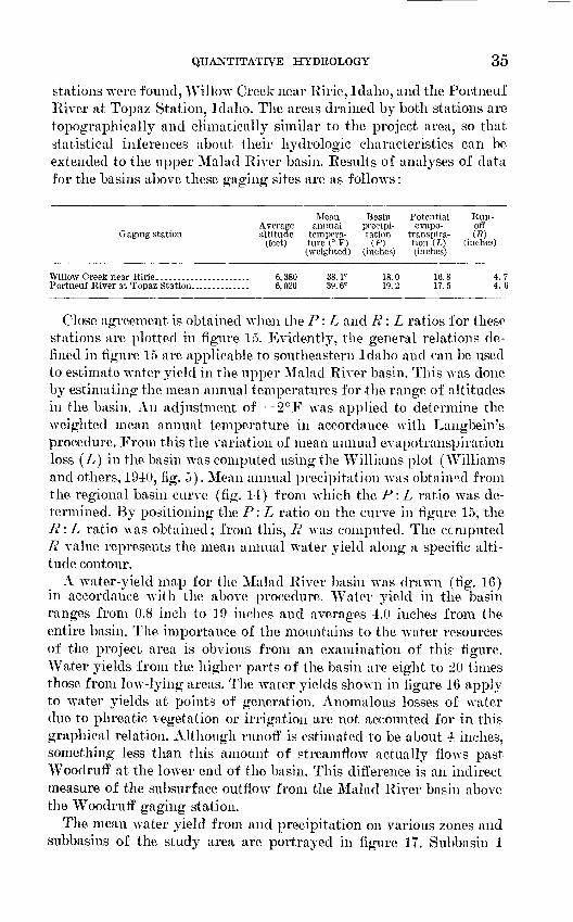
stations were found, "Willow Creek near Eirie, Idaho, and the Portneuf River at Topaz Station, Idaho. The areas drained by both stations are topographically and climatically similar to the project area, so that statistical inferences about their hydrologic characteristics can be extended to the upper Malad River basin. Results of analyses of data for the basins above these gaging sites are as follows:
Gaging stationAveragealtitude
(feet)
_..... 6,380...... 6,020
Meanannual
temperature (° F)(weighted)
38.1°39.6°
Basinprecipitation
(P)(inches)
18.019.2
Potentialevapo-
transpira-tion (L)(inches)
16.817.5
Runoff(R)
(inches)
4. 74.6
Close agreement is obtained when the P: L and R: L ratios for these stations are plotted in figure 15. Evidently, the general relations de fined in figure 15 are applicable to southeastern Idaho and can be used to estimate water yield in the upper Malad River basin. This was done by estimating the mean annual temperatures for the range of altitudes in the basin. An adjustment of 2°F was applied to determine the weighted mean annual temperature in accordance with Langbein's procedure. From this the variation of mean annual evapotranspiration loss (L) in the basin was computed using the Williams plot (Williams and others, 1940, fig. 5). Mean annual precipitation was obtained from the regional basin curve (fig. 14) from which the P:L ratio was de termined. By positioning the P: L ratio on the curve in figure 15, the R:L ratio was obtained; from this, R was computed. The computed R value represents the mean annual water yield along a specific alti tude contour.
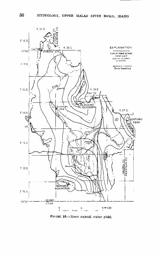
A water-yield map for the Malad River basin was drawn (fig. 16) in accordance with the above procedure. Water yield in the basin ranges from 0.8 inch to 19 inches and averages 4.0 inches from the entire basin. The importance of the mountains to the water resources of the project area is obvious from an examination of this figure. Water yields from the higher parts of the basin are eight to 20 times those from low-lying areas. The water yields shown in figure 16 apply to water yields at points of generation. Anomalous losses of water due to phreatic vegetation or irrigation are not accounted for in this graphical relation. Although runoff is estimated to be about 4 inches, something less than this amount of streamflow actually flows past Woodruff at the lower end of the basin. This difference is an indirect measure of the subsurface outflow from the Malad River basin above the Woodruff gaging station.
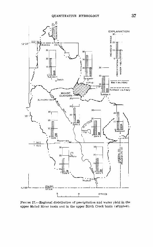
The mean water yield from and precipitation on various zones and subbasins of the study area are portrayed in figure 17. Subbasin 1
36 HYDROLOGY, UPPER MALAD RIVER BASIN, IDAHO
T 10 S
EXPLANATION
T 11 S
T 12S
T 13 S
T 15S
T 16 S
FIGURE 16. Mean annual water yield.
QUANTITATIVE HYDROLOGY 37
/;0.0
.Slg *ll<
EXPLANATION 30
112-30')
1 H roNEIDA CO V Ii; \
4 2° 00
SMILES
FIGURE 17. Regional distribution of precipitation and water yield in the upper Malad River basin and in the upper Birch Creek basin (stippled).
38 HYDROLOGY, UPPER MALAD RIVER BASIN, IDAHO
represents the Little Malad Eiver drainage area above Elkhorn Reser voir (Dam) ; subbasin 2, Birch Creek above transbasin diversion; subbasin 3, Devil Creek above Campbell Creek; and subbasin 4, Deep Creek above Henderson Reservoir. Although Birch Creek is just out side the upper Malad River basin, it has been included in the analyses because most of its flow is diverted into the study area. Mean annual precipitation ranges from a low of 16.0 to a high of 25.4 inches, and annual water yield ranges from 2.4 to 10.4 inches in zone 5 and sub- basin 2, respectively. A 60-percent increase in precipitation between these two subareas resulted in nearly a 450-percent increase in water yield.
GROUND WATER
GEOLOGY IN RELATION TO GROUND WATER
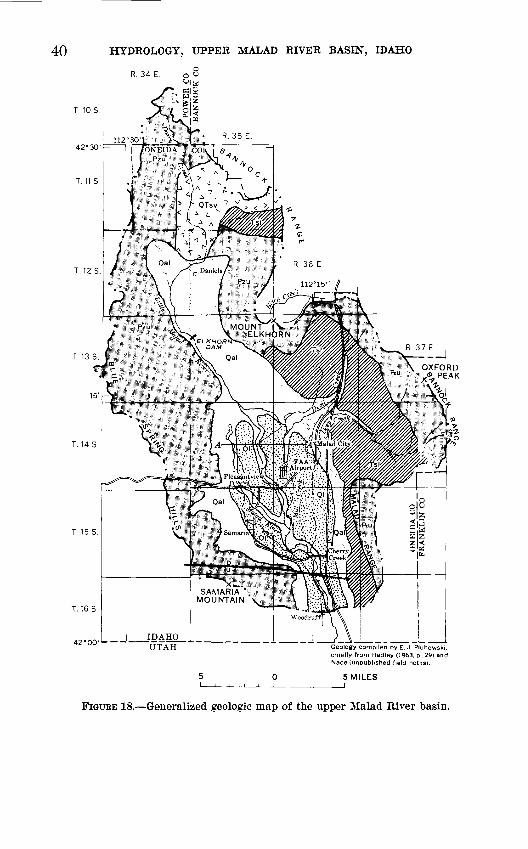
The mountains of the study basin are composed principally of Paleozoic rocks (fig. 18) ranging in age from Cambrian to Permian (Mower and Nace, 1957). Extensive limestone deposits crop out along the Blue Spring Hills in the Wells stratigraphic unit (Piper, 1924). Hadley (1963) reported that the Blue Spring Hills are a series of fault blocks that have been tilted to the southwest. Much of the north ern part of the basin in underlain by the Monroe Canyon and Madison Limestones. The Salt Lake Formation consisting of continental sand stone, shale, and siltstone is extensively exposed along the flanks of the Malad and Bannock Ranges northeast of Malad City.
The Bonneville and Provo shorelines of ancient Lake Bonneville are well defined on foothills surrounding the Malad Valley. A thick sequence of sediments accumulated beneath the lake (the Lake Bonne ville Group) in Quaternary time. This sequence consists of layers, lenses, and tongues of permeable sand and gravel interbedded with less permeable to impermeable beds of silt and clay. The Lake Bonne ville sediments are underlain by sediments of similar characteristics that were deposited by older Quaternary lakes. The aggregate thick ness of the Lake Bonneville Group is not known, but probably does not exceed 50 feet at the deepest points near the middle of the Malad Valley (R. W. Mower, written commun., 1967). Wells exceeding 700 feet in depth do not reach bedrock.
In addition to the lacustrine deposits, alluvial and colluvial deposits accumulated during dry climatic regimes. During dry periods the lake receded beyond the lower boundary of the Malad Vr!ley, and fluvial erosion and deposition took place. Both fine- and coarse-grained materials were deposited by streams as they gradually swung laterally across the valley. Fine-grained materials were washed onto the valley floor from the surrounding uplands by such erosional processes as sheet runoff, soil creep, and gullying. The resulting heterogeneous
GROUND WATER 39
deposit, now hundreds of feet thick, forms the ground-water reservoir. This unconsolidated highly porous geologic unit of widely varying permeability is analogous to a sponge, absorbing much of th°, runoff from the mountains. In this way, the ground-water reservoir partially deters the rapid outflow of water from the area and substantially reduces natural water losses by minimizing the opportunity for evapotranspiration. The ground-water reservoir thereby fulfills the vital function of conserving and storing water for man's use.
THE GROUND-WATER RESERVOIR
The source of much of the economically recoverable ground water in the project area is the thick sequence of unconsolidated alluvial deposits of gravel, sand, silt, and clay underlying the Malad Vrlley and its principal tributary valleys (fig. 18). The gravel and sand beds are of small areal extent, and clay and silt are the dominant materials. A cross section along line A-A' of figure 24 shows the general nature of the deposits in the area west of Malad City (fig. 19). Gravel or sand and gravel alternate irregularly with clay, silt, or clay with gravel; the former are aquifers, strata producing water, and the latter are aquicludes, strata that yield little or no water. The individual beds, such as the sand and gravel at and near the 4,500-foot level in the plotted logs, are not necessarily correlative. Many individual deposits thicken, thin, or pinch out entirely over «, few tens or Kindreds of feet. Water is found in the pore spaces between particles composing the ground-water reservoir. Although fine-grained material such as silt and clay are highly porous, they offer considerable resistance to the movement of water and are very low in permeability. Sand and gravel, on the other hand, are permeable because of their relatively low frictional resistance to water movement.
Ground water occurs under unconfined conditions in the middle and upper parts of the Malad Valley and in the alluvium of most tribu tary valleys. Perched water occurs locally in much of this ar^a in the lenses of sand and gravel that are separated from the main water table by less permeable material. Artesian ground water occurs at depths ranging from a few tens of feet to more than 70 feet south of Malad City, where many wells tap aquifers in the Lake Bonneville Group of Pleistocene age. The Woodruff fault (fig. 18), which trends east-west across the constricted south end of the Malad Valley, is 'a major factor governing flow patterns within the upstream ground- water reservoir. The upthrown southern block of impermeable Paleo zoic sedimentary rocks effectively blocks the downvalley movement of ground water (Nace and Mower, 1957, p. 8). Some of the deeper water-bearing sediments in the Malad Valley probably abut against
40 HYDROLOGY, UPPER MALAD RIVER BASIN, IDAHO
R. 34 E
T 105
T. 11 S
T. 165
Geology compiled by E. J. Pluhowski. chiefly from Hadley (1963, pi.29) and Nace (unpublished field notis).
SMILES
FIGURE 18. Generalized geologic map of the upper Malad River basin.
GROUND WATER 41
the fault block creating artesian conditions in parts of the ground- water reservoir. Considerable upward migration of artesian water takes place through uncased or leaky artesian wells, especially in areas just north of the Woodruff fault and south of a line between Pleasant- view and Malad City.
RECHARGE
The bulk of the recharge to the ground-water reservoir is from direct infiltration of precipitation or surface runoff into the alluvial fans ringing the Malad Valley, from losing streams and canals, and
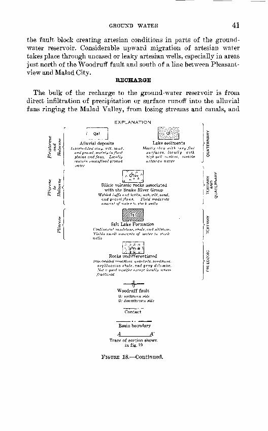
EXPLANATION
Alluvial depositsInterbedded clay, silt, sand,
andgravel, mainly in flood plains and fans. Locally contain unconfined ground water
Lake sedimentsMostly clay with very flat
surfaces, locally with high salt content: contain artesian water
A QTsv A
Silicic volcanic rocks associated with the Snake River Group
Welded tuffs and latite; ash, silt, sand, and gravel flows. Yield moderate amount of water to stock wells
Salt Lake FormationContinental sandstone, shale, and siltstone. Yields small amounts of water to stock wells
Rocks undifferentiatedInterbedded limestone, quartzite, sandstone,
argillaceous shale, and gray dolomite. Not a good aquifer except locally where fractured
D U
Woodruff faultU,' upthrown side D; downthrown side
t <
It V 5
a
Contact
Basin boundary
A______A'Trace of section shown
in fig. 19
FIGURE 18. Continued.
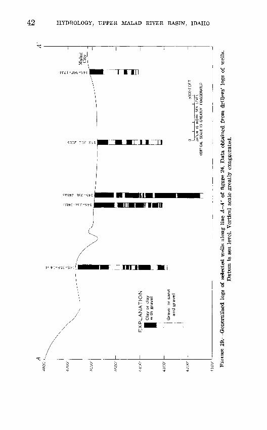
A'
EX
PLA
NA
TIO
N
Cla
y o
r cl
ay
with
gra
vel
Gra
vel
or
sand
and g
rave
l
0 DA
TU
M
IS
ME
AN
S
EA
LE
VE
L V
ER
TIC
AL
SC
ALE
IS
G
RE
AT
LY
EX
AG
GE
RA
TE
D
to
FIG
URE
19.
Gen
eral
ized
log
s of
sel
ecte
d w
ells
alo
ng l
ine
A-A
' of
fig
ure
24.
Dat
a ob
tain
ed f
rom
dri
ller
s' l
ogs
of w
ells
.D
atum
is
sea
leve
l. V
ertic
al s
cale
gre
atly
exa
gger
ated
.

GROUND WATER 43
from unconsumecl irrigation water. Some recharge is received from precipitation that falls on the floor of the Malad Valley and infiltrates downward through the soil zone and the unsaturated zone. However, much of this water is retained as soil moisture and only a small amount reaches the ground-water reservoir. A small quantity of recharge reaches the Malad Valley aquifer system as a consequence of trans- basin diversions of surface water from Birch Creek. The imported water is used for irrigation north of Malad City, and part of it niters downward into the ground-water body.
The alluvial fans surrounding the floor of the Malad Valley are the principal zones of recharge for the underlying aquifer system. The heterogeneous mixture of clay, silt, sand, and gravel composing the alluvial fans laps directly against rocks of Paleozoic age that form the surrounding mountain ranges. Two samples of alluvium were obtained to illustrate in a cursory manner their textural characteristics (fig. 20). Sample 1 is from soil at the base of the exposed alluvium near the western edge of the Malad Valley floor, and sample L is from the upper part of the exposed alluvium southeast of the village of Cherry Creek. The relatively coarse material composing srmple 2, obtained at a point about 500 feet above the valley floor, is in sharp contrast to the predominantly fine-grained material in sample 1. Much of the material near the base of the exposure is very fine sand, silt, and clay, whereas farther upslope coarse sand and gravel predominate. Owing to the highly permeable zone in the upper part of the alluvial fans, runoff from mountain streams and precipitation directly on the alluvium is readily absorbed and transmitted to the ground-water reservoir.
0.5 1.0 2 5 PARTICLE SIZE, IN MILLIMETERS
FIGUEE 20. Particlensize distribution of selected soil samples in the Malad Valley.
367-852 O 70 7
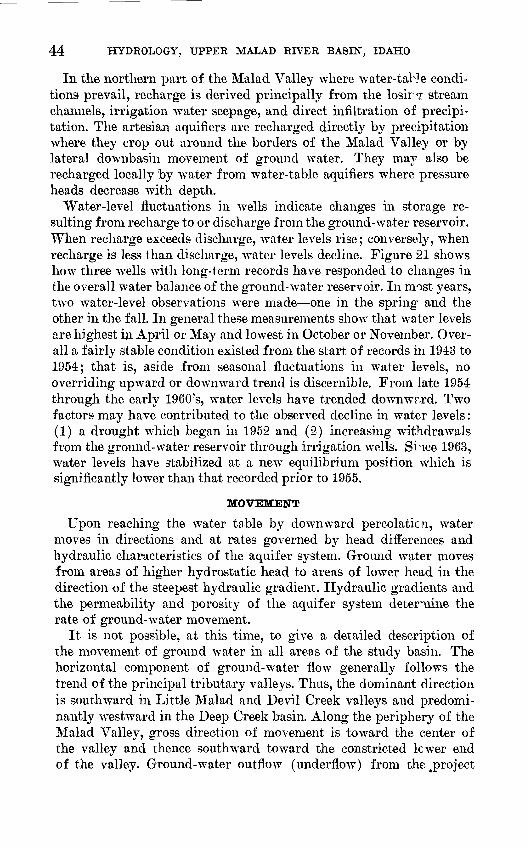
44 HYDROLOGY, UPPER MALAD RIVER BASIN, IDAHO
111 the northern part of the Malad Valley where water-tab]e condi tions prevail, recharge is derived principally from the losir? stream channels, irrigation water seepage, and direct infiltration of precipi tation. The artesian aquifiers are recharged directly by precipitation where they crop out around the borders of the Malad Valley or by lateral downbasin movement of ground water. They may also be recharged locally by water from water-table aquifiers where pressure heads decrease with depth.
Water-level fluctuations in wells indicate changes in storage re sulting from recharge to or discharge from the ground-water reservoir. When recharge exceeds discharge, water levels rise; conversely, when recharge is less than discharge, water levels decline. Figure 21 shows how three wells with long-term records have responded to changes in the overall water balance of the ground-water reservoir. In most years, two water-level observations were made one in the spring- and the other in the fall. In general these measurements show that water levels are highest in April or May and lowest in October or November. Over all a fairly stable condition existed from the start of records in 1943 to 1954; that is, aside from seasonal fluctuations in water levels, no overriding upward or downward trend is discernible. From late 1954 through the early 1960's, water levels have trended downward. Two factors may have contributed to the observed decline in water levels: (1) a drought which began in 1952 and (2) increasing withdrawals from the ground-water reservoir through irrigation wells. Since 1963, water levels have stabilized at a new equilibrium position which is significantly lower than that recorded prior to 1955.
MOVEMENT
Upon reaching the water table by downward percolatic n, water moves in directions and at rates governed by head differences and hydraulic characteristics of the aquifer system. Ground water moves from areas of higher hydrostatic head to areas of lower head in the direction of the steepest hydraulic gradient. Hydraulic gradients and the permeability and porosity of the aquifer system determine the rate of ground-water movement.
It is not possible, at this time, to give a detailed description of the movement of ground water in all areas of the study basin. The horizontal component of ground-water flow generally follows the trend of the principal tributary valleys. Thus, the dominant direction is southward in Little Malad and Devil Creek valleys and predomi nantly westward in the Deep Creek basin. Along the periphery of the Malad Valley, gross direction of movement is toward the center of the valley and thence southward toward the constricted kwer end of the valley. Ground-water outflow (underflow) from the ^project

GROUND WATER 45
area is southward paralleling the movement of the Malad River (fig. 3).
The vertical component of ground-water movement is predomi nantly downward in all recharge areas, particularly where the artesian aquifers crop out near the uplands flanking the Malad Valley. There may be considerable migration of water along bedding planes and some around well casings. A large -amount of upward migration of water occurs near wells penetrating the artesian aquifers. Thermal springs in the vicinity of the Woodruff fault suggests the existence of upward movement of ground water deep within the reservoir for some distance north of the fault. Downstream from the fault to the lower boundary of the project area, ground water probably moves horizontally with a slight upward component locally.
DISCHARGE
Ground water is discharged from the basin by seepage to streams, evapotranspiration, springs, underflow, and pumping. The rate at which it is discharged depends on many interrelated factors includ ing season of the year, volume of recharge, intensity of pumping, soil and aquifer characteristics, and vegetal cover. Ground-water discharge to the Malad River, to springs, and as underflow is at a maximum from March to May; it is at a minimum from September to November. Evapotranspiration and pumpage are greatest in sum mer and least in winter.
In contrast to virtually all stream reaches in the Malad Valley, the Malad River between Cherry Creek Lane and the Woodruff gaging station is a gaining reach. For example, the discharge of the river on August 1, 1962, at Cherry Creek Lane was 0.80 cfs (cubic feet per second), whereas it was 17.0 cfs at the Woodruff gage at out 4% miles downstream. These measurements represent dry-weatl Q,r flow so that they reflect ground-water discharge to the reach. O^ing to seepage losses upstream and substantial diversions for irrigation, summer flow in the Malad River is often very small at the Cherry Creek Lane site. Much of the gain in flow below Cherry Cre^vk Lane enters the river from Woodruff Springs located 2 miles above the Malad River gaging station and about 1 mile south of the Woodruff fault. As previously noted, the fault acts as a barrier to ground-water movement. The springs and seeps in the reach of the Malad River between Cherry Creek Lane and the gaging station discharge highly mineralized ground water. The close proximity of Woodruff Springs to the Woodruff fault suggests that the springs may derive part of their discharge from an upward flow pattern within the ground-water reservoir created by the fault.
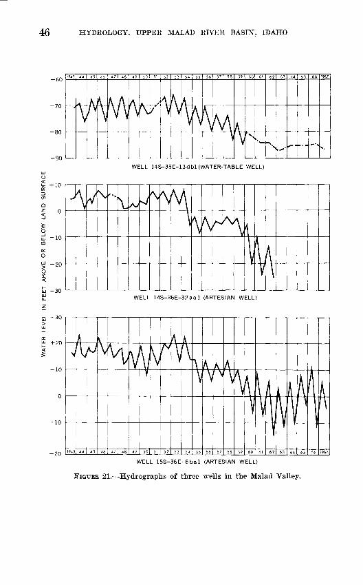
W
WA
TE
R
LEV
EL,
IN
F
EE
T
AB
OV
E
OR
B
ELO
W
LA
ND
S
UR
FA
CE
+
+
I I
I +
r\3
co
oo
ro
*"
'-'o
o
o
o
o
o
o
Oi
E z:
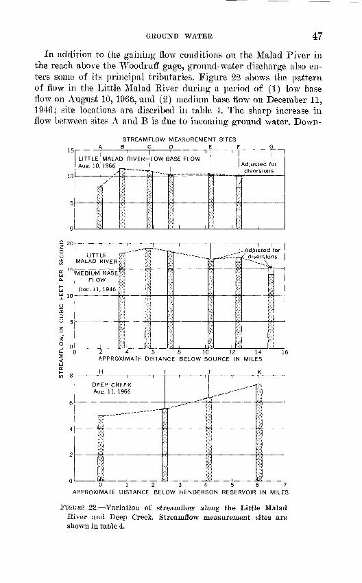
GROUND WATER 47
In addition to the gaining flow conditions on the Malad Piver in the reach above the Woodruff gage, ground-water discharge also en ters some of its principal tributaries. Figure 22 shows the pattern of flow in the Little Malad River during a period of (1) low base flow on August 10, 1966, and (2) medium base flow on December 11, 1946; site locations are discribed in table <±. The sharp increase in flow between sites A and B is due to incoming ground water. Down-
STREAMFLOW MEASUREMENT SITES BCD E F
10
LITTLE Aug. 10
1 MALA 1966
P
i
1D
i
1 |ll RIVER LOW BASE FLOW
J
||1 1 : .
« |
Adjusted for diversions
/
'1 I
O oLJJOT tr 15LJJ Q.
LJJ
£ 100mD 0 5z
°> n
i
LITTLE MALAD RIVER
MEDIUM BASE FLOW
Dec. 11, 1946
l
i6
'm
1
1
1
'?S$
1
1~~~" r ?---.-
[
' >. ;
"-
1
1
i511sm
4
>st
i-Adjusted for / diversionsi "¥
5
|
1 ]:
ill
t o 2 4 6 8 10 12 14 APPROXIMATE DISTANCE BELOW SOURCE, IN MILES
16
OT 8
DEEP CREEK Aug. 11, 1966
0123456 7 APPROXIMATE DISTANCE BELOW HENDERSON RESERVOIR, IN MILF.S
FIGURE 22. Variation of streamflow along the Little Malad River and Deep Creek. Streamflow measurement sites are shown in table 4.

48 HYDROLOGY, UPPER MALAD RIVER BASIN, IDAHO
stream from site B (gaging station) streamflow declined slightly, indicating seepage loss. The seepage run on December 11, 1946, shows the same pattern except that gaining conditions extended somewhat further downstream. Along Deep Creek a steady outflow of ground water is apparent in the downstream direction. This condition prob ably is characteristic of the stream, because a protracted drought had reduced ground-water levels sharply prior to the seepage run. De spite the substantial loss of recharge, ground-water levels in the Deep Creek valley remained higher than stream stages and the result was a continued outflow of water from the aquifer to the creek. The bulk of the water supply for Malad City is derived from a series of in filtration galleries that intercept the flow of ground water before it reaches Deep Creek in the vicinity of site J (fig. 22 and table 4). The intercepted water is conveyed to a detention reservoir from which it is pumped to the city for distribution.
TABLE 4. Streamflow measurement sites along the Little Malad River and Deep Creek
Identifi- Statlon name cation
letter in fig. 24
Little Malad Eiver above ELkhorn Eeser- B voir (Dam).
Little Malad Eiver below Elkhorn Beser- voir (Dam).....----.....--..--..........- C
Little Malad Eiver at Jones Eanch . ........ DLittle Malad Eiver above Sand Eid?e ditch. E Little Malad Eiver below St. Johns Canal.. F Little Malad Eiver at Sand Eidge damsite.. G
Deep Creek below Henderson Eeservoir. . . . H Deep Creek above Malad City water-supply
Distance in miles i Quarter
1. 9 SWJiNWJi 3.6 SEMSEM
i. 3 NW&SWJ!10.4 NEkNEjJ 12. 5 NEJaSEJ<£ 15.0 NE>|SE^
0 NWJiNEJi
2. 9 NWJiSE^ 4.3 SWjiNEJ^ 6. 1 SWMSW&
Location
Section
26 35
7 17 33
3 14
18
2 10 15
T^own- st ip (S.)
1212
13 13 13 14 14
14
14 14 14
Eange (E.)
34 34
35 35 35 35 35
37
36 36 36
i Distances given are below the source for the Little Malad Biver and below Henderson Eeservoir for Deep Creek.
Widespread salinization of soils is evident in the lower Malad Valley because of evapotranspiration from the ground-water reservoir. Water is withdrawn by direct evaporation if the capillary fringe is at or near land surface. The height to which capillary water rises depends largely upon the spacing between individual particles. The fire-grained material throughout the Malad Valley permits water to rise well above the wrater table by capillary action; if this water reaches near the land surface, it is subject to evaporation. The rate at which ground water is lost to the atmosphere is governed by the same climatic factors that affect evaporation from free-water surfaces. Water is also withdrawn from the ground-water reservoir wherever plant roots penetrate the water table or the capillary zone. Salts in the evaporated water that are left behind in the soil zone at or near land surface tend to accumu-
GROUND WATER 49
late there as the evaporated water is replaced by upward moving capil lary water. The salts cannot move downward against the rising water and no leaching by infiltrating precipitation is possible. Concentration of certain salts causes a reduction in soil permeability and hardening of the soil. Crops cannot be grown economically under these conditions, and the land eventually becomes unproductive.
Some loss of productive land may be due to the increased use of irrigation water. However, most of the unproductive acreage in the project area consists of saline and alkaline soils resulting from ground- water evapotranspiration, principally in the lower Malad Valley. In other words, owing to the natural salinization of soils stemming from ground-water evapotranspiration, some sections of the lower Malad Valley were unsuited to agriculture long before the advent of civilization.
UNDERFLOW
Ground-water outflow^ (underflow) from the upper Malad Biver basin in the vicinity of the Woodruff gaging station can be estimated by use of the following water-balance equation for the bas'n:
Input=output ± change in storage (1)
where, for the purposes of this study, change in storage may be ne glected owing to the long period of record (1931-60) used in the analysis.
A small amount of surface water is imported into the study area from Birch Creek by way of a transbasin diversion channel. Aside from this flow, there is no evidence of any other importatior of water from outside the basin. Precipitation in its various forms is clearly the basin's major source of water. Inflow to the basin, therefore, con sists oi precipitation plus the relatively small quantity imported from Birch Creek. Outflow from the basin consists of evapotranspiration, surface-water outflow at Woodruff, and underflow. Substituting these factors in equation 1 and neglecting storage change over the long term, the equation is:
Precipitation+imported water= evapotranspiration + surface-water outflow + underflow
(2)
Solving for underflow and transposing terms:
Underflow = precipitation evapotranspiration surface-water outflow + imported water
(3)
50 HYDROLOGY, UPPER MALAD RIVER BASIN, IDAHO
The first two terms on the right-hand side of equation 3 are equiv alent to water yield, or water that is available as surface runoff or ground-water recharge after evapotranspiration demands have been satisfied. A fair estimate of water yield may be obtained using Lang- bein's method; however, his ratio plot (fig. 15) is based largely on areas that are free of excessive losses due to irrigation. Irrigation is widespread in the Malad Valley, so the substantial water looses stem ming from irrigation must be included in the water-balance equation. Equation 3 can therefore be restated as follows:
U=WY-IL-SWO+IW (4) where U= underflow
WY= water yieldIL = net loss due to irrigation
SWO = surface-water outflowIW= imported water (from Birch Creek)
Each of the items on the right-hand side of equation 4 can be quantita tively evaluated so that it is possible to obtain a fair estimate of ground-water underflow.
According to a Department of Agriculture census, about 22,000 acres was irrigated in the Malad Valley in 1959. If potential evapo transpiration is assumed to approximate irrigation-water looses, then an estimate of such losses can be made. Potential evapotranspiration in the Malad Valley is about 24 inches as computed by the Thornthwaite (1948) method. Therefore about 44,000 acre-feet of water was con sumptively used in 1959 for irrigation in the basin, but this is not the actual water loss due to irrigation. The actual loss from the irriga ted lands is that amount remaining after "effective" precipitation during the growing season is subtracted from the water loss originat ing from irrigation (44,000 acre-feet). Effective precipitation is rain fall that infiltrates into the soil and becomes available to crc^s in the form of soil moisture. Total rainfall during the growing season (May 15-Sept. 30) is 4.6 inches, of which only 2 inches is estimated to be available to crops. Accordingly, the loss of water due to irrigation is 24 inches minus 2 inches, or 22 inches (40,000 acre-feet) annually.
The annual water yield of the basin is 4 inches, or about 115,000 acre-feet for the 485 square-mile basin above the Woodruff gaging station. On the basis of two discharge measurements and tH record of flow at Devil Creek above Campbell Creek, transbasin imports of flow from Birch Creek are estimated to average 4,000 acre-feet annu ally. Surface-water outflow from the basin consists of an average annual discharge in the Malad River of 61 cfs (44,000 acre-feet) and an estimated flow of 7,000 acre-feet in the Warm Springs Canal which bypasses the Woodruff gaging station; therefore, the total annual
SURFACE WATER 51
surface-water outflow is about 51,000 acre-feet. Each factor in the right-hand side of equation 4 has now been quantitatively evaluated. Substituting- the computed values in equation 4 gives:
Underflow=115,000 - 40,000 - 51,000+4,000=28,000 acre-feet
The total outflow^ (water yield) from the upper Malad River basin, above Woodruff, is 51,000 acre-feet of surface water plus 28,000 acre- feet of ground water, or about 79,000 acre-feet. For the basin, Mower and Nace (1957) estimated that about 37,000 acre-feet of water is consumed annually by phreatic vegetation. Clearly, a substantial part of the total water resources of the basin is being consumed by water- loving vegetation. Control or eradication of the undesirable phreatic growths or replacement with beneficial crops represents a major area for improvement in the basin's water balance. A substantial reduction in water loss could be gained by careful application of water to irri gated crops so that only water actually needed for optimum growth and soil flushing is provided. Elimination of water losses due to phreatic growths plus reduction of irrigation losses by optimal appli cation of water to crops could conceivably result in a 50-percent increase in the beneficial water use of the basin.
SURFACE WATER
The earliest measurements of streamflow in the upper Malad River basin were probably those made during the period 1911-13 on the Little Malad River. The first systematic attempt to measure streamflow in the basin was made during the 1932 water year (a 12-month period begin ning Oct. 1 and ending the following Sept. 30) with the establishment of water-stage recorders on six streams. Since that time, about 150 station-years of record (through 1967) have been collected and about half of this represents the combined records of three stations namely, Malad River at Woodruff, Little Malad River above Elkhorn Reser voir (Dam), and Devil Creek above Campbell Creek. During the 1930's, stream-gaging activities were concentrated on Deep Creek, a major tributary to the east of Malad City, and Devil Creek which drains a large area north of the city. These streams were gaged to evaluate their potential as possible sites for water-supply reservoirs. Currently (1968), only two stations are still in operation, Malad River at Woodruff and Little Malad River above Elkhorn Reservoir (Dam). The gaging station on Deep Creek was discontinued in 1949 8 f ter com pletion of Henderson Reservoir just upstream from the gag°. Miscel laneous discharge measurements were made principally during the late 1940's, in 1962, and in 1966. In all, streamflow at 38 sites has been measured either continuously through the use of recorders or inter-

ST
RE
AM
A
ND
L
OC
AT
ION
1 2 3 4 5 6 7 8 9
10
11
12
13
14
15
16
17
18 19
20
21
22
23
24
25 27 29 31
32
33
34 3
6
37
38
m
o
i i
ma
mm
mi
mr3
mm
mm
mm
mfm
ml
mm
mT
i MM
I
mm
mm
m
.^S
WM
D
n n aZ
)
ED a a a
CD
I I
1 1
1 1
I I
C
mm
mm
m
jge
ai
a
mm mm
m_-
i
en a a a n a n a a d a a en
Mala
d R
iver
at
sp
rin
gs,
near
Mala
d C
ity
Mala
d R
iver
be
low
sp
rin
gs,
near
Mala
d C
ity
Mala
d R
ive
r near
Ma
lad
City
Mala
d R
iver
near
Ple
asa
ntv
iew
Mala
d R
ive
r at
Ple
asantv
iew
Mala
d R
iver
near
Sa
ma
ria
(above
Gw
en
ford
Mill
ditch)
Gw
en
ford
Mill
ditch
near
Sa
ma
ria
Mala
d R
iver
near
Sa
ma
ria
(belo
w G
we
nfo
rd M
ill d
itch
)M
ala
d R
iver
near
Sa
ma
ria
(2
mile
s b
elo
w G
we
nfo
rd M
ill d
itch)
Ma
in C
an
al
near
Sa
ma
ria
(2
mile
s b
elo
w G
wenfo
rd M
ill d
itch)
Div
ers
ion
canal
near
Sa
ma
ria
(div
ert
s f
rom
Main
Canal)
Wa
rm S
prin
gs C
an
al
near
Sa
ma
ria
Wa
rm S
prin
gs C
an
al
near
Wo
od
ruff
Wa
rm S
prings C
an
al
at
Woodru
ffL
ittle
Mala
d R
ive
r b
elo
w s
prin
gs,
near
Da
nie
lsD
airy C
ree
k near
Da
nie
lsW
right
Cre
ek
near
Da
nie
ls
Little M
ala
d R
iver
ab
ove
Elk
horn
Re
se
rvo
ir (
Dam
), n
ear
Ma
lad
City
Little M
ala
d R
iver
be
low
E
lkh
orn
R
eserv
oir (
Dam
), n
ear
Mala
d C
ity
Little M
ala
d R
iver
at
Ed
Jones R
anch
, near
Mala
d C
ityLittle M
ala
d R
iver
at
Sand R
idg
e d
itch
, near
Mala
d C
ity
Sand R
idg
e d
itch n
ear
Ma
lad
City
St.
Johns C
an
al
near
Ma
lad
City
Little M
ala
d R
ive
r b
elo
w S
t. J
ohns C
an
al
headin
g,
near
Mala
d C
ity
Little
Mala
d R
ive
r near
Ple
asa
ntv
iew
Devi
l C
reek
be
low
Birch
Cre
ek
div
ers
ion, near
Mala
d C
ity
Devi
l C
reek
above
Eva
ns
div
iders
, near
Mala
d C
ity
Da
vis
Cre
ek
at
sourc
e,
near
Mala
d C
ity
Devi
l C
reek
near
Ma
lad
City
Mill
Cre
ek
be
low
Eva
ns
div
iders
, near
Mala
d C
ity
Th
ird
Cre
ek
near
Ma
lad
City
De
ep
Cre
ek
at
Mala
d C
ity
Mala
d R
ive
r at
Cherr
y C
reek L
an
e,
near
Wo
od
ruff
M
ala
d R
ive
r at
Woodru
ff
EX
PL
AN
AT
ION
Co
ntin
uo
us r
eco
rds
Occa
sio
na
l dis
charg
e
me
asu
rem
en
ts o
nly
Oi to 53 M
ft) §
CO
19
35
1
94
0
1945
\^
WA
TE
R
YE
AR
E
ND
ING
n 1
95
5
1Q6D
SE
PT
EM
BE
R
30
FIGT
JBE
23. L
engt
h of
str
eam
-gag
ing
reco
rds.
Num
bers
on
left
ref
er to
site
s sh
own
in f
igur
e 24
.
SURFACE WATER 53
mittently by miscellaneous discharge measurements. Following the severe flood of February 1962, indirect measurements of p°,ak dis charge were made on several streams in the basin.
The length and type of streamflow record available at each site are shown in figure 23. Locations of the discharge-measurement sites are indicated in figure 24, and pertinent descriptive data are srown on pages 55-57. Daily discharge records for gaging stations in th°i Malad River basin and the results of discharge measurements of partial- record stations are published in U.S. Geological Survey water-supply papers titled "Surface Water Supply of the United States, Prrt 10."
Surface-water resources have, almost from the start, played a key role in the argicultural development of the Malad River basin. Shortly after the base flow of streams had been exhausted, numerous detention reservoirs were built to store runoff. The largest of these, Henderson Reservoir on Deep Creek, is used for irrigation and recreation. There is a small public water-supply detention basin just north of Malad City; however, virtually all other reservoirs in the project area were built to supply water for irrigation.
With one exception, all reservoirs have functioned satisfactorily. Owing to the presence of cavernous limestone deposits at the Elkhorn damsite (about 14 miles northwest of Malad City), the reservoir would not hold water except for brief periods following her.vy run off. In the spring of 1966, construction was begun on a new reservoir on the Little Malad River at a point about 4 miles above the Elkhorn damsite. A considerable effort was made to eliminate underf ow past the damsite by grouting concrete deep into the streambed and the flanking hill slopes. Construction on the project was nearing comple tion in 1967. Thus, no appraisal of the success of this venture will be possible in the near future. If the project is a success, then part of the spring runoff can be stored for later use during the irrigation season. The storage of water that has virtually gone unusei in the past will permit substantial expansion of irrigated acreage in the Little Malad River valley by providing water for land that previously was used for grazing and dryfarming.
LOW-FLOW CHARACTERISTICS OF STREAMS
One of the principal goals of water management in the project area involves detaining as much of the spring runoff as possible in efficient reservoirs. In addition to a comprehensive appraisal of the subsurface geology of a proposed damsite, detailed information on the amount and variability of streamflow is also needed. In particular, the water
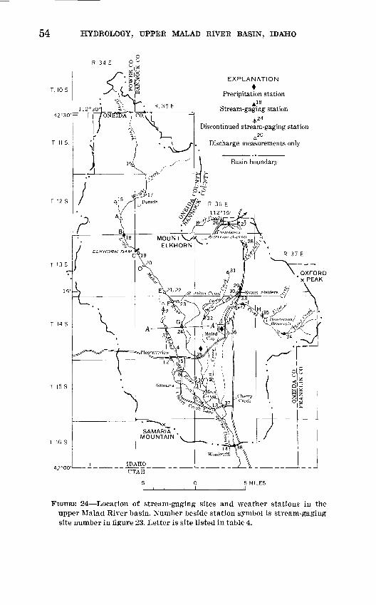
54 HYDROLOGY, UPPER MALAD RIVER BASIN, IDAHO
R 34 E
T. 105.
T 11 S.
EXPLANATION
Precipitation station
A 18Stream-gaging station
424 Discontinued stream-gaging station
A20
Discharge measurements only
Basin boundary
T 12 S
T. 135
T 145
T 15 S
T 16 S
FIGURE 24 Location of stream-gaging sites and weather stations in the upper Malad River basin. Number beside station symbol is stream-gaging site number in figure 23. Letter is site listed in table 4.
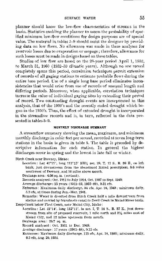
SURFACE WATER 55
planner should know the low-flow characteristics of streairs in the basin. Statistics enabling the planner to assess the probability of spec ified minimum low-flow conditions for design purposes are of special value. The material in tables 5-9 should assist the designer by provid ing data on low flows. No allowance was made in these analyses for reservoir losses due to evaporation or seepage; therefore, allowance for such losses must be made in designs based on these tables.
Studies of low flow are based on the 28-year period April 1, 1932, to March 31, 1960 (1932-59 climatic years). Although no one record completely spans this period, correlation techniques permit extension of records of all gaging stations to estimate probable flows during the entire base period. Use of a single long base period eliminates incon sistencies that would arise from use of records of unequal length and differing periods. Moreover, when applicable, correlation techniques increase the value of individual gaging sites by extending their period of record. Two outstanding drought events are incorporated in this analysis, that of the 1930's and the recently ended drought which be gan in the 1950's. Thus, the effect of extended drought is incorporated in the streamflow records and is, in turn, reflected in the data pre sented in tables 5-9.
MONTHLY DISCHARGE SUMMARY
A streamflow summary showing the mean, maximum, and minimum monthly discharge in cubic feet per second, recorded at seven long-term stations in the basin is given in table 5. The table is preceded by de scriptive information for each station. In general the highest discharges occur in spring and the lowest in late fall or winter.
Birch Creek near Downey, Idaho:Location: Lat 42°21', long 112°15' SEi/4 sec. 28, T. 12 S., R. 36 E., on left
bank, just downstream from the abandoned Malad powerplant, 8.6 milessouthwest of Downey, and 10 miles above mouth.
Drainage area : 6v56,sq- m. (revised).Records analyzed: Oct. 1911 to July 1914, Oct. 1937 to Sept. 1949. Average discharge: 13 years (1911-12, 1937-49), 9.31 cfs. Extremes: Maximum daily discharge, 34 cfs, Apr. 24, 1943; minimum daily,
5.2 cfs, at times during Jan.-Mar. 1941. Remarks: Water is diverted from Birch Creek half a mile downstream from
station and carried by transbasin canal to Devil Creek in Malad River basin. Deep Creek below First Creek, near Malad City, Idaho:
Location: Lat 42°14', long 112°11', in sec. 7, T. 14 S., R. 37 E., just down stream from site of proposed reservoir, 1 mile north and 3% miles east ofMalad City, and 12 miles upstream from mouth.
Drainage area: 29.7 sq. m. Record analyzed: Oct. 1931 to Dec. 1948. Average discharge: 17 years (1931-48), 9.11 cfs. Extremes : Maximum daily discharge, 113 cfs, Apr. 18, 1936; minimum daily,
0.3 cfs, Aug. 29,1934.
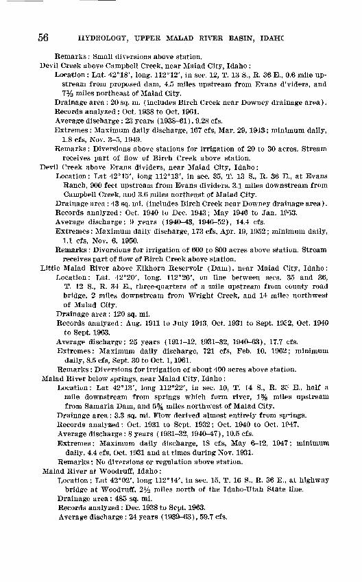
56 HYDROLOGY, UPPER MALAD RIVER BASIN, IDAHC
Remarks: Small diversions above station. Devil Creek above Campbell Creek, near Malad City, Idaho :
Location : Lat. 42°18', long. 112° 12', in sec. 12, T. 13 S., R. 36 E., 0.6 mile up stream from proposed dam, 4.5 miles upstream from Evans d'viders, and7y2 miles northeast of Malad City.
Drainage area : 20 sq. m. (includes Birch Creek near Downey drainage area). Records analyzed : Oct. 1938 to Oct. 1961. Average discharge : 23 years (1938-61), 9.28 cfs. Extremes: Maximum daily discharge, 167 cfs, Mar. 29, 1943; minimum daily,
1.8 cfs, Nov. 3-5, 1949. Remarks: Diversions above stations for irrigation of 20 to 30 acres. Stream
receives part of flow of Birch Creek above station. Devil Creek above Evans dividers, near Malad City, Idaho:
Location: Lat 42°15', long 112°13', in sec. 35, T. 13 S., R. 36 II, at EvansRanch, 900 feet upstream from Evans dividers, 3.1 miles downstream fromCampbell Creek, and 3.6 miles northeast of Malad City.
Drainage area : 43 sq. mi. (includes Birch Creek near Downey drainage area). Records analyzed: Oct. 1940 to Dec. 1943; May 1946 to Jan. 1953. Average discharge: 9 years (1940-43, 1946-52), 14.4 cfs. Extremes: Maximum daily discharge, 173 cfs, Apr. 19, 1952; minimum daily,
1.1 cfs, Nov. 6, 1950. Remarks : Diversions for irrigation of 600 to 800 acres above station. Stream
receives part of flow of Birch Creek above station.Little Malad River above Elkhorn Reservoir (Dam), near Malad City, Idaho:
Location: Lat. 42°20', long. 112°26', on line between sees. 35 and 36,T. 12 S., R. 34 E., three-quarters of a mile upstream from county roadbridge, 2 miles downstream from Wright Creek, and 14 mile? northwestof Malad City.
Drainage area : 120 sq. mi. Records analyzed: Aug. 1911 to July 1913, Oct. 1931 to Sept. 19S2, Oct. 1940
to Sept. 1963.Average discharge: 25 years (1911-12, 1931-32, 1940-63), 17.7 cfs. Extremes: Maximum daily discharge, 721 cfs, Feb. 10, 1962; minimum
daily, 8.5 cfs, Sept. 30 to Oct. 1,1961.Remarks: Diversions for irrigation of about 400 acres above station.
Malad River below springs, near Malad City, Idaho :Location: Lat 42°13', long 112°22', in sec. 10, T: 14 S., R. 3e E., half a
mile downstream from springs which form river, 1% miles upstream from Samaria Dam, and 5% miles northwest, of Malad City.
Drainage area: 3.3 sq. mi. Flow derived almost entirely from springs. Records analyzed: Oct. 1931 to Sept. 1932; Oct. 1940 to Oct. 1947. Average discharge : 8 years (1931-32, 1940-47), 10.5 cfs. Extremes: Maximum daily discharge, 18 cfs, May 6-12, 1947; minimum
daily, 4.4 cfs, Oct. 1931 and at times during Nov. 1931. Remarks: No diversions or regulation above station.
Malad River at Woodruff, Idaho :Location: Lat 42°02', long 112°14', in sec. 15, T. 16 S., R. 36 E., at highway
bridge at Woodruff, 2 1/4 miles north of the Idaho-Utah State line. Drainage area : 485 sq. mi. Records analyzed: Dec. 1938 to Sept. 1963. Average discharge : 24 years (1939-63), 59.7 cfs.
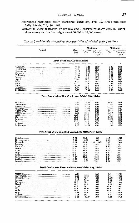
SURFACE WATER 57
Extremes: Maximum daily discharge, 2,240 efs, Feb. 12, 1962; minimum daily, 8.0 cfs, July 16,1960.
Remarks: Flow regulated by several small reservoirs above station. Diver sions above station for irrigation of 20,000 to 25,000 acres.
TABLE 5. Monthly sir earn flow chafacteristics of selected gaging stations
Month Mean (cfs)
Maximum
Cfs Calendar year
Minimum
Cfe Calendar year
Birch Creek near Downey, Idaho
July............
.. ......................-....... 7.65
.................................. 7.51
................................... 7.16
.................................... 7.15
. .._-....--..--.........__..._ 7.53
.................................... 12.4
.-...--..__--.._ ..__.-....--. 16.2_._....--._..-..._.-.....-......... 12.7.................................... 9.39.................................... 8.44.................................... 7.98
9.45 9.40 9.14 8.86
10.3 11.1 23.6 21.1 17.6 11.8 10.1 9.56
Deep Creek below First Creek, near Malad City,
January--.-....
July.. ..........
.................................... 3.05
................................... 3.00
.................................... 2.97
..... rr . ............................ 2.99
.................................... 3.80
.................................... 7.07
.................................... 22.1
.................................... 26.9
.................................... 17.7
.-_...... -.._..........--.-.... 10.8--....--.--.....-...--....-....-...- 5.56.................................... 3.02
5.48 4.74 4.85 3.96 7.70
16.4 58.9 51.2 30.4 14.9 11.5 8.20
1912 1912 1911 1912 1912 1912 1943 1912 1912 1945 1945 1912
Idaho
1946 1946 1945 1946 1943 1943 1936 1932 1945 1937 1937 1945
5.42 5.24 4.28 5.22 5.34 6.06 8.69 9.94 7.54 6.97 6.53 6.37
0.97 1.43 1.34 1.90 2.34 3.52 4.64 3.03 2.08
.84
.44
.52
1913 1913 1913 1914 1914 1914 1945 1939 1939 1940 1940 1913
1934 1934 1931 1936 1937 1944 1934 1934 1934 1934 1934 1934
Devil Creek above Campbell Creek, near Malad City, Idaho
July.........----.
.................................... 7.01---...-.-...-........--..--.....-..- 7.44.................................... 7.64.................................... 7.59
......-.-...----...-.-.........---.. 11.5
.................................... 17.5
.................................... 10.47 ^7
. . -. -....-.-.. ....--.. 6.62
.................................... 6.45
10. 3 1950 9. 95 1951
10.0 1951, 1952 9. 82 1952
11. 6 1947 25. 5 1943 46. 4 1952 23. 8 1952 21. 7 1945 11. 1 1950 9. 29 1952 8. 99 1951
4.47 4.98 5.22 5.2? 4.8P 6.05 4.9F 5. If 4.5f 4.5F 4. 40 3.92
1960 1959 1959 1957 1956 1961 1961 1961 1961 1961 1960 1961
Devil Creek above Evans dividers, near Malad City, Idaho
July... .----....
Seotember ....
.................................... 9.12
.................................... 9.77
.................................... 9.91
.................................... 9.85
.................................... 11.0
.................................... 17.5
.................................... 40.2
...--.---.-....-.-...-.-............ 26.4
......... .............. .......... 14.7
.................................... 9.34
.................................... 7.74
.................................... 7.31
11.5 12.3 13.1 12.5 18.1 35.3 76.7 40.0 23.4 14.9 10.7 9.10
1950 1950 1950 1951 1947 1943 1952 1952 1950 1950 1950 1950
6.5 7.61 7.52 7.60 7.67 9 18
17.4 18 0 10 0 7.11 5 47 6.29
1940 1942 1940 1942 1949 1942 1947 1947 1941 1949 1949 1942
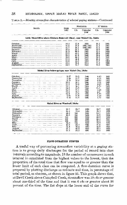
58 HYDROLOGY, UPPER MALAD RIVER BASIN, IDAHO
TABLE 5. Monthly streamflow characteristics of selected gaging stations Continued
Month Mean (cfs)
Maximum M'limum
Cfs Calendar year
Cfs Calendar year
Little Malad River above Elkhorn Reservoir (Dam), near Malad City, Idaho
October _ .......................November. ..--...-....---....-..December............. ..........January. ........................February... .....................March ......----...-.-...---.....April.. ..._......................May.. ---..-----..---------...--.June.............................July............................AUgUSt ----.---.-..--.-__---.....September- ......................
................... 14.2
................... 14.5
..-.....-.-.--.--.. 14.7
................... 15.3
................... 21.3
..... ...----.---.. 22.2--- --._-.---. 23.2..---..--.--....... 20.0..-.....---...-.... 17.3-.------..--.. 15.8..-...-.-.-...-.... 14.6-.-.--....-..--.... 13.9
17.817.618.122.188.050.541.334.224.821.222.417.7
19521950, 19521945, 1952
196219621962194819521912191219121952
10.111.111.512.012.513.613.912.510.811.711.310.0
196119611961196119321932196119611961196319631961
Malad River below springs, near Malad City, Idaho
October. -.___.-..__.-_._..__.-__November.. ............... ......December. ......................January. ........................February. .......................March.....---....---............April............................May. .,---------------...-.-._---June......... --------------------July....----..............--.--..August -.--.--------..-.-----..--September.......................
..-....--...--..... 8.07
...--__..-.-......- 7.99
................... 8.74
..........-..---.. 10.0
................... 11.0
..--... ..- 12.1 -.--..- .---.- 13.4-_.-..........--- 14.0-.---.-.-.-_--.---- 12.0...--...-.....-.... 10.2.-.-.... ........ 9.51................... 9.15
10.511.713.814.113.414.115.517.114.111.911.811.0
194619451945194619441944194619461945194619461946
4.404.7*6.3?7.518.899.75
11.19. 908.07. 507.197.77
193119311931194219411942194219321932193219321932
Malad River at Woodruff, Idaho
October.........................November .......................December.... ________ .........January. _-_.---_..-____________.February. .......................March...........................April. ...........................May.............................June.... ....-_-....--_-..........July..-.-..----........-........AUgUSt ---------.----.-..--..---.S eptember. .-------..............
.................... 32.7
.....-_. . .-._. 56.4
.-.___..._.-..--._.. 69.0
.................... 66.5
..._._..._.____-_... 116
......._..........-. 129
.................... 103
.................... 53.2
..........._..--.... 32.3
..-...--...._....... 21.4
.................... 21.7
.................... 21.2
53.799.4
19415045024928011489.233.440.329.2
195219461946195319621946195219501945195219521951
18.725.932.128.348.949.335.618.815.314.313.915.2
196219621962196319601961196119611961196219631963
FLOW-DURATION CURVES
A useful way of portraying streamflow variability at a gaging sta tion is to group daily discharges for the period of record into class intervals according to magnitude. If the number of occurrences in each interval is cumulated from the highest values to the lowest, then the proportion of the total time that flow was equal to or greater than the lower limit of each class can be computed. A flow-duration curve is prepared by plotting discharge as ordinate and time, in percentage of total period, as abscissa, as shown in figure 25. This graph shows that, at Devil Creek above Campbell Creek, streamflow was 10 cfs o*1 greater about one-third of the time and that it was 6 cfs or greater about 90 percent of the time. The flat slope at the lower end of the cnrve for
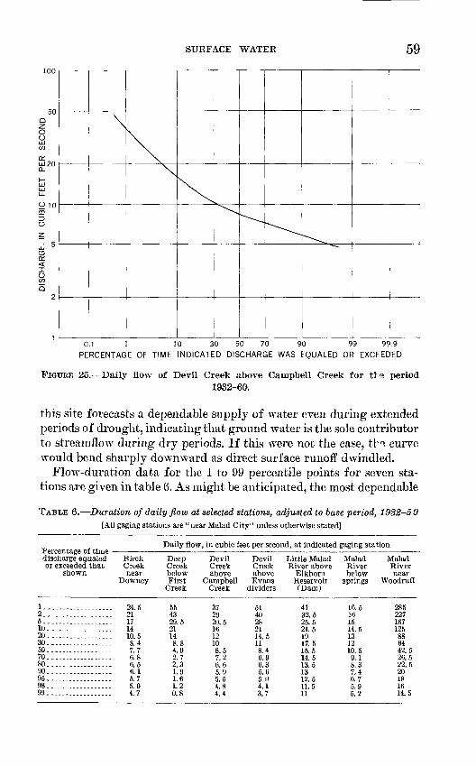
SURFACE WATER 59100
120
010
0.1 1 10 30 50 70 90 99 99.9
PERCENTAGE OF TIME INDICATED DISCHARGE WAS EQUALED OR EXCEEDED
FIGURE 25. Daily flow of Devil Creek above Campbell Creek for tl-"> period1932-60.
this site forecasts a dependable supply of water even during extended periods of drought, indicating that ground water is the sole contributor to streamflow during dry periods. If this were not the case, th Q< curve would bend sharply downward as direct surface runoff dwindled.
Flow-duration data for the 1 to 99 percentile points for seven sta tions are given in table 6. As might be anticipated, the most dependable
TABLE 6. Duration of daily flow at selected stations, adjusted to base period, 1932-59[All gaging stations are "near Malad City" unless otherwise stated]
Daily flow, in cubic feet per second, at indicated gaging station
discharge equaledor exceeded that
shown
BirchCreeknear
Downey
DeepCreekbelowFirst
Creek
DevilCreekabove
CampbellCreek
DevilCreekaboveEvans
dividers
Little MaladRiver above
ElkhomReservoir(Dam)
MaladRiverbelow
springs
MaladRivernear
Woodruff
24.521171410.58.47.76.86.56.15.75.04.7
554329.521148.84.02.72.31.91.61.20.8
372920.51612108.57.26.65.95.54.84.4
5140282114.5118.46.96.35.65.04.13.7
4132.525.521.51917.515.514.513.51312.511.511
16.5161514.5131210.59.18.37.46.75.95.2
285227167125886442.526.522.520181614.5
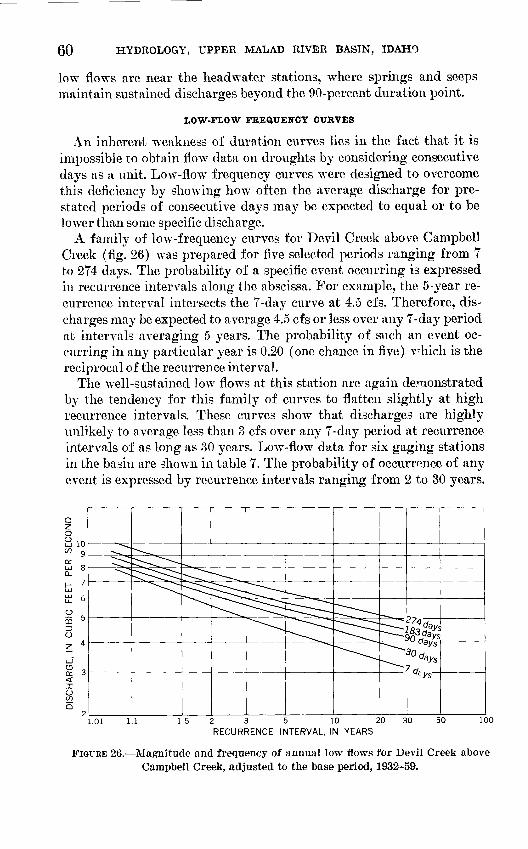
60 HYDROLOGY, UPPER MALAD RIVER BASIN, IDAHO
low flows are near the headwater stations, where springs and seeps maintain sustained discharges beyond the 90-percent duration point.
LOW-FLOW FREQUENCY CURVES
An inherent weakness of duration curves lies in the fact that it is impossible to obtain flow data on droughts by considering consecutive days as a unit. Low-flow frequency curves were designed to overcome this deficiency by showing how often the average discharge for pre- stated periods of consecutive days may be expected to equal or to be lower than some specific discharge.
A family of low-frequency curves for Devil Creek above Campbell Creek (fig. 26) was prepared for five selected periods ranging from 7 to 274 days. The probability of a specific event occurring is expressed in recurrence intervals along the abscissa. For example, the 5-year re currence interval intersects the 7-day curve at 4.5 cfs. Therefore, dis charges may be expected to average 4.5 cfs or less over any 7-day period at intervals averaging 5 years. The probability of such an event oc curring in any particular year is 0.20 (one chance in five) which is the reciprocal of the recurrence interval.
The well-sustained low flows at this station are again demonstrated by the tendency for this family of curves to flatten slightly at high recurrence intervals. These curves show that discharges are highly unlikely to average less than 3 cfs over any 7-day period at recurrence intervals of as long as 30 years. Low-flow data for six gaging stations in the basin are shown in table 7. The probability of occurrence of any event is expressed by recurrence intervals ranging from 2 to 30 years.
1.5 235 10 20 RECURRENCE INTERVAL, IN YEARS
50 100
FIGURE 26. Magnitude and frequency of annual low flows for Devil Creek above Campbell Creek, adjusted to the base period, 1932-59.
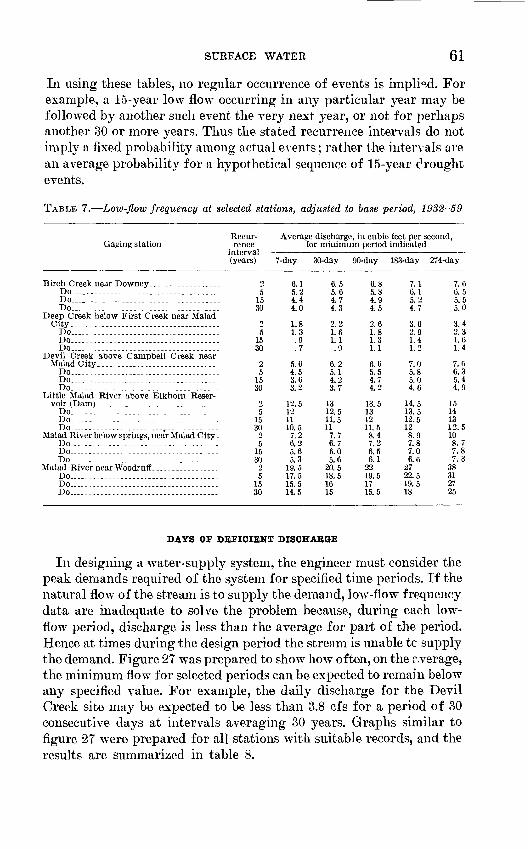
SURFACE WATER 61
In using these tables, no regular occurrence of events is implied. For example, a 15-year low flow occurring in any particular year may be followed by another such event the very next year, or not for perhaps another 30 or more years. Thus the stated recurrence intervals do not imply a fixed probability among actual events; rather the intervals are an average probability for a hypothetical sequence of 15-year brought events.
TABLE 7. Low-flow frequency at selected stations, adjusted to base period, 1932-59
Recur- G aging station rence
interval (years)
Do.. ............................... ....Do.....-.-.--.-.... ..-....--.___....._.Do .-.... ............ --._.. ......
Deep Creek below First Creek near Malad City---..---...-...-........-.............
Do.. ................................. ...Do.. ...--.--.-.----.-....-............. -Do.-.-------..-..-.---.-.----....-.--...
Devil Creek above Campbell Creek near Malad City. --.-.......-...---...----.... .
Do......................................Do... ....... ........ ....... .......... ..Do. . --.--.. -.-.._. ..--....-.-..-.
Little Malad River above Elkhorn Reser-
Do....... ...............................Do. ........ ........---..--.--..-.--...--Do --.. . ...... .,- -.-.
Malad River below springs, near Malad City. Do _ ..-----.-----.......-........_....Do......................................Do......................................
Malad River near Woodruff-. .........._....Do......................................Do......................................Do. --.......-.--....--........-......
2 5
15 30
2 5
15 30
2 5
15 30
2 5
15 30
5 15 30
25
15 30
Average discharge, in cubic feet per second, for minimum period indicated
7-day 30-day 90-day 183-day 274-day
6.1 5.2 4.4 4.0
1.8 1.3 .9.7
5.6 4.5 3.6 3.2
12.5 12 11 10.5 7.2 6.2 5.6 5.3
19.5 17.5 15.5 14.5
6.5 5.6 4.7 4.3
2.2 1.6 1.1 .9
6.2 5.1 4.2 3.7
13 12.5 11.5 11 7.7 6.7 6.0 5.6
20.5 18.5 16 15
6.8 5.8 4.9 4.5
2.6 1.8 1.3 1.1
6.6 5.54.7 4.2
13.5 13 12 11.5 8.4 7.2 6.5 6.1
22 19.5 17 15.5
7.1 6.1 5.2 4.7
3.0 2.0 1.4 1.2
7.0 5.8 5.0 4.6
14.5 13.5 12.5 12 8.9 7.8 7.0 6.6
27 22.5 19.5 18
7.6 6.5 5.5 5.0
3.4 2.3 1.6 1.4
7.6 6.3 5.4 4.9
15 14 13 12.5 10 8.7 7.8 7.3
38 31 27 25
DAYS OF DEFICIENT DISCHARGE
111 designing a water-supply system, the engineer must consider the peak demands required of the system for specified time periods. If the natural flow of the stream is to supply the demand, low-flow frequency data are inadequate to solve the problem because, during each low- flow period, discharge is less than the average for part of the period. Hence at times during the design period the stream is unable tc supply the demand. Figure 27 was prepared to show how often, on the average, the minimum flow for selected periods can be expected to remain below any specified value. For example, the daily discharge for the Devil Creek site may be expected to be less than 3.8 cfs for a period of 30 consecutive days at intervals averaging 30 years. Graphs similar to figure 27 were prepared for all stations with suitable records, and the results are summarized in table 8.
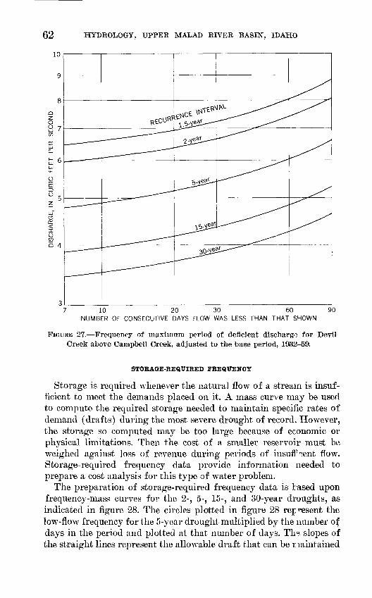
62 HYDROLOGY, UPPER MALAD RIVER BASIN, IDAHO
7 10 20 30 60NUMBER OF CONSECUTIVE DAYS FLOW WAS LESS THAN THAT SHOWN
FIGURE 27. Frequency of maximum period of deficient discharge for Devil Creek above Campbell Creek, adjusted to the base period, 1932-59.
STORAGE-REQUIRED FREQUENCY
Storage is required whenever the natural flow of a stream is insuf ficient to meet the demands placed on it. A mass curve may be used to compute the required storage needed to maintain specific rates of demand (drafts) during the most severe drought of record. However, the storage so computed may be too large because of economic or physical limitations. Then the cost of a smaller reservoir must be weighed against loss of revenue during periods of insuff ",ent flow. Storage-required frequency data provide information needed to prepare a cost analysis for this type of water problem.
The preparation of storage-required frequency data is based upon frequency-mass curves for the 2-, 5-, 15-, and 30-year droughts, as indicated in figure 28. The circles plotted in figure 28 rep^sent the low-flow frequency for the 5-year drought multiplied by the number of days in the period and plotted at that number of days. ThQ, slopes of the straight lines represent the allowable draft that can be maintained

SURFACE WATER 63
TABLE 8. Annual low-flow frequency for days of deficient discharge at selected stations, adjusted to base period, 1932-59
Gaging station
Discharge, in cubic feet per second, Recurrence below which flow remained con-
interval tinuous for length of mininum period (years) indicated
7-day 30-day 60-day 90-day
Birch Creek near Downey.. ....... ...................Do........ ........................................Do.......-..... ...............................Do... ....... . .. -.. ....... . . ....
Deep Creek below First Creek near Malad City _ ...Do.... ............................................Do .Do . .-.---. ...... ... ...
Devil Creek above Campbell Creek near Malad City.Do ....... .. .. . ... .......Do.......................... ...................Do . . - ..
Little Malad River above Elkhorn Reservoir (Dam),near Malad C ity -- --. -
Do....... .............-.........-.....-.......Do .Do .
Malad River below springs, near Malad City. --------Do. .-.-...-...-................ ...........Do ..Do
Malad River at Woodruff... - . . .Do...-- . ........ -..__..-.__......._.-... ...Do Do
25
1530
25
153025
1530
25
1530
25
1530
25
1530
6.35.34.64.12.11.51.0.8
6.04.83.93.4
13121110.57.56.55.85.5
2017.515.514.5
6.65.64.84.32.81.91.31.06.65.44.43.8
13.512.51211.58.47.26.56.1
21.5191716
7.16.05.14.63.22.21.51.27.36.C4.84.2
14.513.512.5129.07.87.16.6
2420.518.517
7.56.45.44.93.72.41.61.38.16.65.24.6
15.5141312.59.88.37.57.0
272219.518
100 150 200 250 300 PERIOD OF MINIMUM DISCHARGE, IN DAYS
FIGURE 28. Frequency-mass curve and storage-draft lines for Devil Creek above Campbell Creek for the 5-year recurrence interval, adjusted to the 1932-59 base period.
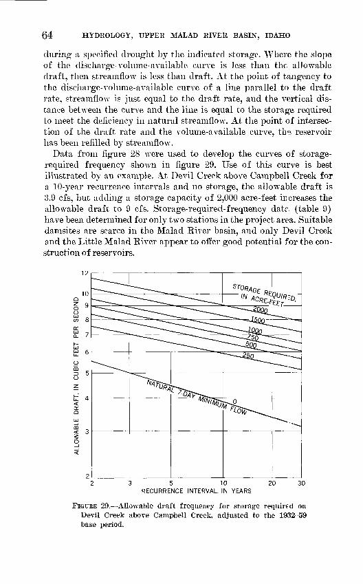
64 HYDROLOGY, UPPER MALAD RIVER BASIN, IDAHO
during a specified drought by tho indicated storage. Where the slope of the discharge-volume-available curve is less than the allowable draft, then streamflow is less than draft. At the point of tangency to the discharge-volume-available curve of a line parallel to the draft rate, streamflow is just equal to the draft rate, and the vertical dis tance between the curve and the line is equal to the storage required to meet the deficiency in natural streamflow. At the point of intersec tion of the draft rate and the volume-available curve, tli 0, reservoir has been refilled by streamflow.
Data from figure 28 were used to develop the curves of storage- required frequency shown in figure 29. Use of this curve is best illustrated by an example. At Devil Creek above Campbell Creek for a 10-year recurrence intervals and no storage, the allowable draft is 3.9 cfs, but adding a storage capacity of 2,000 acre-feet in creases the allowable draft to 9 cfs. Storage-required-frequency datr, (table 9) have been determined for only two stations in the project area. Suitable damsites are scarce in the Malad Eiver basin, and only Devil Creek and the Little Malad Eiver appear to offer good potential for the con struction of reservoirs.
5 10 RECURRENCE INTERVAL, IN YEARS
20 30
FIGURE 29. Allowable draft frequency for storage required on Devil Creek above Campbell Creek, adjusted to the 1932-59 base period.
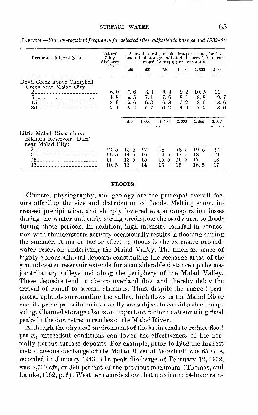
SURFACE WATER 65
TABLE 9. Storage-required frequency for selected sites, adjusted to base period 1932-59
Recurrence interval (years)Natural Allowable draft, in cubic feet per second, for the
7-day amount of storage indicated, in acre-feet, uncor- discharge rected for seepage or evaporation
(cfs)250 500 750 1,000 1,500 2,000
Devil Creek above Campbell Creek near Malad City:
6. 04. 83. 93.4
7. 66. 55. 65. 2
8. 37. 16. 35. 7
8.97. 66. 86.2
9.28. 17.26.6
10. 58. 88. 07. 3
119. 78. 68.0
500 1,000 1,500 2,000 2,500 3,000
Little Malad River above Elkhorn Reservoir (Dam) near Malad City:
25 ____________15---_--_----_30 ________ _
_________ 12._________ 11._________ 11
10.
55
5
15. 514. 513. 513
17161514
18161515
55
18171616
555
19181716
20191817
FLOODS
Climate, physiography, and geology are the principal overall fac tors affecting the size and distribution of floods. Melting snow, in creased precipitation, and sharply lowered evapotranspiration losses during the winter and early spring predispose the study area to floods during those periods. In addition, high-intensity rainfall in connec tion with thunderstorm activity occasionally results in flooding during the summer. A major factor affecting floods is the extensive ground- water reservoir underlying the Malad Valley. The thick sequence of highly porous alluvial deposits constituting the recharge area? of the ground-water reservoir extends for a considerable distance up the ma jor tributary valleys and along the periphery of the Malad Valley. These deposits tend to absorb overland flow and thereby delay the arrival of runoff to stream channels. Thus, despite the rugged peri pheral uplands surrounding the valley, high flows in the Malad River and its principal tributaries usually are subject to considerable damp ening. Channel storage also is an important factor in attenuatirg flood peaks in the downstream reaches of the Malad River.
Although the physical environment of the basin tends to reduce flood peaks, antecedent conditions can lower the effectiveness of the nor mally porous surface deposits. For example, prior to 1962 the highest instantaneous discharge of the Malad River at Woodruff was 650 cfs, recorded in January 1943. The peak discharge of February 12, 1962, was 2,530 cfs, or 390 percent of the previous maximum (Thomas, and Lamke, 1962, p. 6). Weather records show that maximum 24-hour rain-
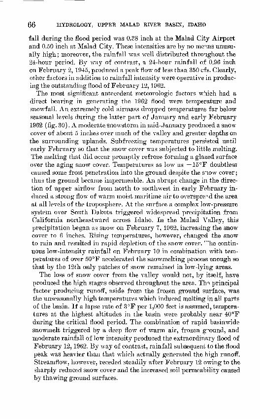
66 HYDROLOGY, UPPER MALAD RIVER BASEST, IDAHO
fall during the flood period was 0.38 inch at the Malad City Airport and 0.50 inch at Malad City. These intensities are by no me-'vns unusu ally high; moreover, the rainfall was well distributed throughout the 24-hour period. By way of contrast, a 24-hour rainfall of 0.96 inch on February 2, 1945, produced a peak flow of less than 350 cfs. Clearly, other factors in addition to rainfall intensity were operative in produc ing the outstanding flood of February 12,1962.
The most significant antecedent meteorologic factors which had a direct bearing in generating the 1962 flood were temperature and snowfall. An extremely cold airmass dropped temperatures far below seasonal levels during the latter part of January and early February 1962 (fig. 30). A moderate snowstorm in mid-January produced a snow cover of about 5 inches over much of the valley and greater depths on the surrounding uplands. Sub freezing temperatures persisted until early February so that the snow cover was subjected to little melting. The melting that did occur promptly refroze forming a glazed surface over the aging snow cover. Temperatures as low as 15°F doubtless caused some frost penetration into the ground despite the snow cover; thus the ground became impermeable. An abrupt change in the direc tion of upper airflow from north to southwest in early February in duced a strong flow of warm moist maritime air to overspread the area at all levels of the troposphere. At the surface a complex low-pressure system over South Dakota triggered widespread precipitation from California northeastward across Idaho. In the Malad Valley, this precipitation began as snow on February 7, 1962, increasing the snow cover to 6 inches. Rising temperatures, however, changed the snow to rain and resulted in rapid depletion of the snow cover. The contin uous low-intensity rainfall on February 10 in combination with tem peratures of over 50°F accelerated the snowmelting process enough so that by the 12th only patches of snow remained in low-lying areas.
The loss of snow cover from the valley would not, by itself, have produced the high stages observed throughout the area. Th^ principal factor producing runoff, aside from the frozen ground surface, was the unseasonally high temperatures which induced melting in all parts of the basin. If a lapse rate of 3°F per 1,000 feet is assumed, tempera tures at the highest altitudes in the basin were probably near 40°F during the critical flood period. The combination of rapid basinwide snowmelt triggered by a deep flow of warm air, frozen ground, and moderate rainfall of low intensity produced the extraordinary flood of February 12,1962. By way of contrast, rainfall subsequent to the flood peak was heavier than that which actually generated the high runoff. Streamflow, however, receded steadily after February 12 owing to the sharply reduced snow cover and the increased soil permeability caused by thawing ground surfaces.
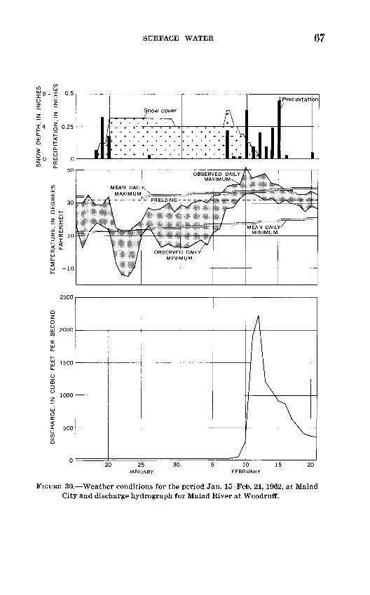
SURFACE WATER 67
Z4 tLJ Q
io w
rl 0.5
0.25 ~1.1 + + +
Snow coverl+-+-+-\
l+\
i:-|-> ,1,1Precipitation/
II
2500
1500
1000
20 25 JANUARY
30 10 FEBRUARY
15 20
FIGURE 30. Weather conditions for the period Jan. 15-Feb. 21,1962, at Malad City and discharge hydrograph for Malad River at Woodruff.

68 HYDROLOGY, UPPER MALAD RIVER BASEST, IDAHO
FLOOD FREQUENCY
The flood of February 12, 1962, was a very rare event which could be evaluated statistically if sufficiently long records were available. Unfortunately, streamflow records in the upper Malad Elver basin are far too short to permit an accurate appraisal of the frequency of recurrence of floods of this magnitude. Nevertheless, the records are of sufficient length to provide valuable information on the magnitude and frequency of floods having recurrence intervals as long r,s 50 years. Knowledge of the flood characteristics of streams provides a basis for designing structures to be located on their flood plains. Economic considerations dictate the choice of a design frequency; however, an evaluation of these economic factors is beyond the scope of this report.
On the basis of available records, the period 1939-63 was selected as the base period for flood analysis. Five stations have records of sufficient length for use in the analysis. Only one station was in operation through the base period; records for the other stations were extended by correlation with nearby stations.
PLOTTING POSITION
The analysis of floodflows starts with a listing of all annual peak discharges at a gaging station. These are ranked according to mag nitude starting with the highest flood as 1. Plotting positions (recur rence intervals) for each flood were computed by using the formula
RI= > where RI is the recurrence interval, n is the number of m
years of record, and m is the order number.Annual floods are plotted against recurrence interval on a special
form devised by Powell (1943), and the resulting curve of relation is a straight line for all stations used in this report. The recurrence inter val of a flood does not imply any regularity of occurrence; rather it is the average time that a given flood will be equaled or exceeded during a long period of time.
MEAN ANNUAL FLOOD
The mean annual flood at a given station is the arithmetic mean of the annual peak discharges in an infinitely long series of such events. The recurrence interval of the mean annual flood is 2.33 years, accord ing to the theory of extreme values as applied to floods by Gumbel (1945). The 2.33-year flood can be determined graphically and is the mean annual flood used in this report.
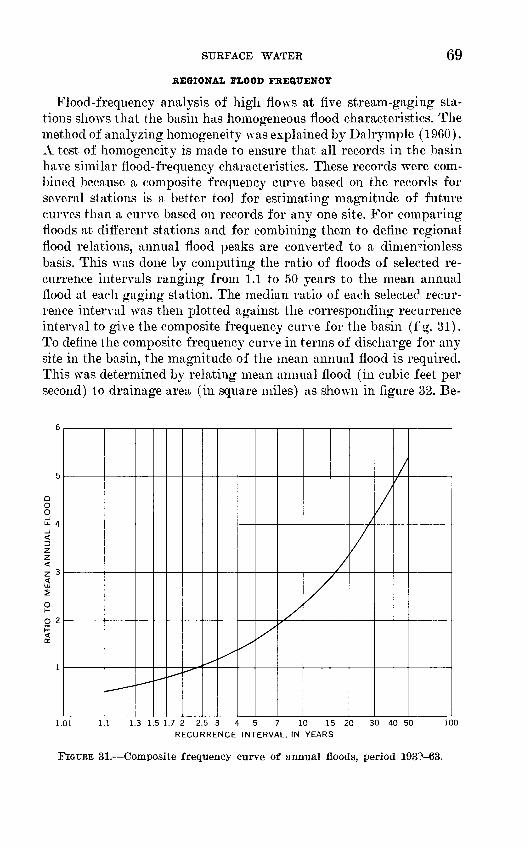
SURFACE WATER 69
REGIONAL FLOOD FREQUENCY
Flood-frequency analysis of high flows at five stream-gaging sta tions shows that the basin has homogeneous flood characteristics. The method of analyzing homogeneity was explained by Dalrymple (1960). A test of homogeneity is made to ensure that all records in the basin have similar flood-frequency characteristics. These records were com bined because a composite frequency curve based on the records for several stations is a better tool for estimating magnitude of future curves than a curve based on records for any one site. For comparing floods at different stations and for combining them to define regional flood relations, annual flood peaks are converted to a dimen^ionless basis. This was done by computing the ratio of floods of selected re currence intervals ranging from 1.1 to 50 years to the mean annual flood at each gaging station. The median ratio of each selectee1 recur rence interval was then plotted against the corresponding recurrence interval to give the composite frequency curve for the basin (f g. 31). To define the composite frequency curve in terms of discharge for any site in the basin, the magnitude of the mean annual flood is required. This was determined by relating mean annual flood (in cubic feet per second) to drainage area (in square miles) as shown in figure 32. Be
O 2
1.01 1.1 1.3 1.5 1.7 2 2.5 3 4 5 7 10 15 20 RECURRENCE INTERVAL, IN YEARS
30 40 50 100
FIGURE 31. Composite frequency curve of annual floods, period 193?-63.
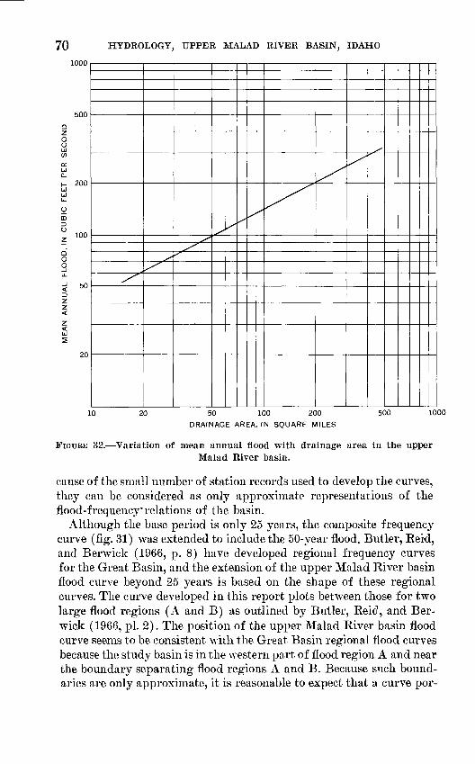
70 HYDROLOGY, UPPER MALAD RIVER BASIN, IDAHO
1000
500
200
100
50
20
10 20 50 100 200
DRAINAGE AREA, IN SQUARE MILES
500 1000
FIGUEE 32. Variation of mean annual flood with drainage area in the upperMalad River basin.
cause of the small number of station records used to develop the curves, they can be considered as only approximate representations of the flood-frequency* relations of the basin.
Although the base period is only 25 years, the composite frequency curve (fig. 31) was extended to include the 50-year flood. Butler, Reid, and Berwick (1966, p. 8) have developed regional frequency curves for the Great Basin, and the extension of the upper Malad Jliver basin flood curve beyond 25 years is based on the shape of these regional curves. The curve developed in this report plots between those for two large flood regions (A and B) as outlined by Butler, Reic1 , and Ber wick (1966, pi. 2). The position of the upper Malad River basin flood curve seems to be consistent with the Great Basin regional flood curves because the study basin is in the western part of flood region A and near the boundary separating flood regions A and B. Because such bound aries are only approximate, it is reasonable to expect that a curve por-
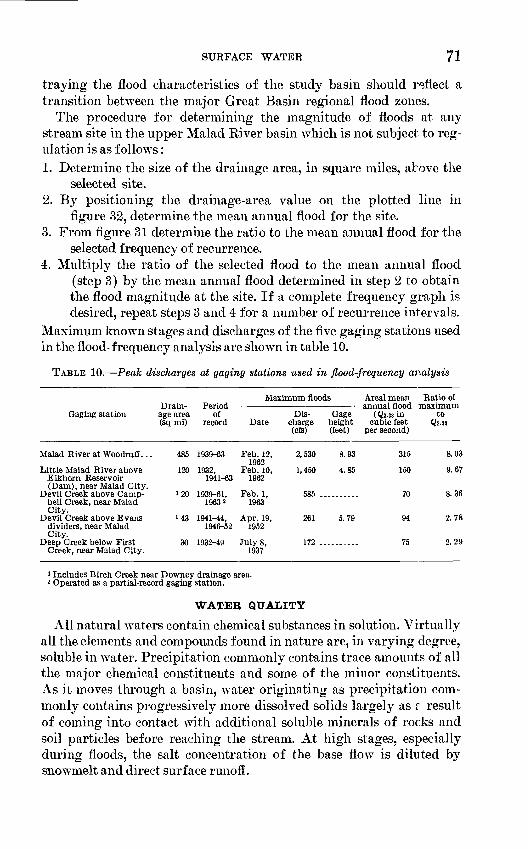
SURFACE WATER 71
traying the flood characteristics of the study basin should reflect a transition between the major Great Basin regional flood zones.
The procedure for determining the magnitude of floods at any stream site in the upper Malad River basin which is not subject to reg ulation is as follows:1. Determine the size of the drainage area, in square miles, above the
selected site.2. By positioning the drainage-area value on the plotted line in
figure 32, determine the mean annual flood for the site.3. From figure 31 determine the ratio to the mean annual flood for the
selected frequency of recurrence.4. Multiply the ratio of the selected flood to the mean annual flood
(step 3) by the mean annual flood determined in step 2 to obtain the flood magnitude at the site. If a complete frequency graph is desired, repeat steps 3 and 4 for a number of recurrence intervals.
Maximum known stages and discharges of the five gaging stations usedin the flood-frequency analysis are shown in table 10.
TABLE 10. Peak discharges at gaging stations used in flood-frequency analysis
Drain- Period Gaging station age area of
(sq mi) record
Malad River at Woodruff. ..
Little Malad River above Elkhorn Reservoir (Dam), near Malad City.
Devil Creek above Camp bell Creek, near Malad City.
Devil Creek above Evans dividers, near Malad City.
Deep Creek below First Creek, near Malad City.
485 1939-63
120 1932, 1941-63
120 1939-61, 19632
'43 1941-14, 1946-52
30 1932-49
Maximum floods An
Dis- Gage ( Date charge height ci
(cfs) (feet) per
Feb. 12, 2, 530 8. 93 1962
Feb. 10, 1, 450 4. 85 1962
Feb. 1, 585 ..........1963
Apr. 19, 261 5. 79 1952
1937
sal mean Ratio of ual flood maximum Qs.33 in to ibic feet Q2.33 second)
315 8. 03
150 9. 67
70 8. 36
94 2. 78
75 2. 29
1 Includes Birch Creek near Downey drainage area.2 Operated as a partial-record gaging station.
WATER QUALITY
All natural waters contain chemical substances in solution. Virtually all the elements and compounds found in nature are, in varying degree, soluble in water. Precipitation commonly contains trace amounts of all the major chemical constituents and some of the minor constituents. As it moves through a basin, water originating as precipitation com monly contains progressively more dissolved solids largely as r result of coming into contact with additional soluble minerals of rocks and soil particles before reaching the stream. At high stages, especially during floods, the salt concentration of the base flow is diluted by snowmelt and direct surface runoff.
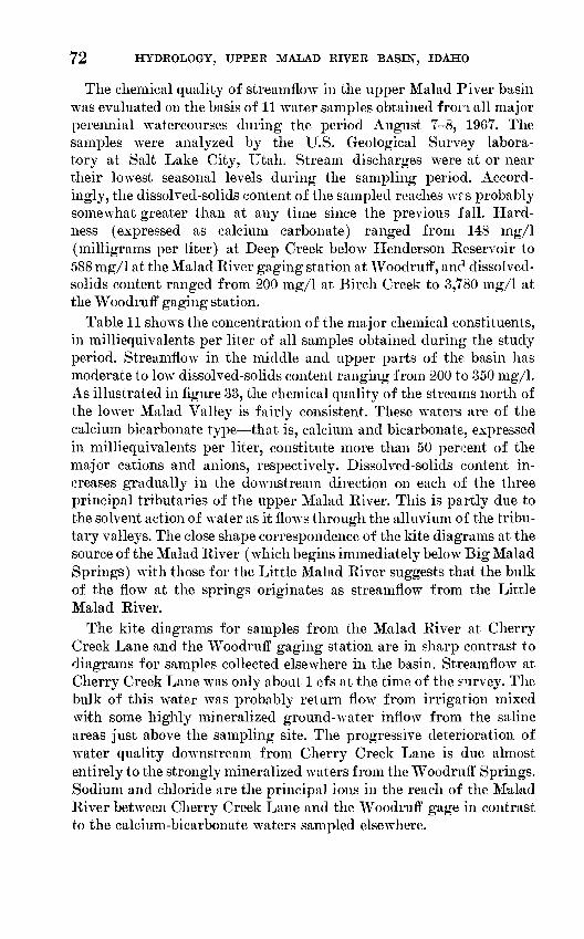
72 HYDROLOGY, UPPER MALAD RIVER BASIN, IDAHO
The chemical quality of streamflow in the upper Malad Piver basin was evaluated on the basis of 11 water samples obtained from all major perennial watercourses during the period August 7-8, 1967. The samples were analyzed by the U.S. Geological Survey labora tory at Salt Lake City, Utah. Stream discharges were at or near their lowest seasonal levels during the sampling period. Accord ingly, the dissolved-solids content of the sampled reaches WPS probably somewhat greater than at any time since the previous fall. Hard ness (expressed as calcium carbonate) ranged from 148 mg/1 (milligrams per liter) at Deep Creek below Henderson Keservoir to 588 mg/1 at the Malad Kiver gaging station at Woodruff, anc1 dissolved- solids content ranged from 200 mg/1 at Birch Creek to 3,780 mg/1 at the Woodruff gaging station.
Table 11 shows the concentration of the major chemical constituents, in milliequivalents per liter of all samples obtained during the study period. Streamflow in the middle and upper parts of the basin has moderate to low dissolved-solids content ranging from 200 to 350 mg/1. As illustrated in figure 33, the chemical quality of the streams north of the lower Malad Valley is fairly consistent. These waters are of the calcium bicarbonate type that is, calcium and bicarbonate, expressed in milliequivalents per liter, constitute more than 50 percent of the major cations and anions, respectively. Dissolved-solids content in creases gradually in the downstream direction on each of the three principal tributaries of the upper Malad River. This is partly due to the solvent action of water as it flows through the alluvium of the tribu tary valleys. The close shape correspondence of the kite diagrams at the source of the Malad River (which begins immediately below Big Malad Springs) with those for the Little Malad River suggests that the bulk of the flow at the springs originates as streamflow from the Little Malad River.
The kite diagrams for samples from the Malad River at Cherry Creek Lane and the Woodruff gaging station are in sharp contrast to diagrams for samples collected elsewhere in the basin. Streamflow at Cherry Creek Lane was only about 1 cfs at the time of the survey. The bulk of this water was probably return flow from irrigation mixed with some highly mineralized ground-water inflow from the saline areas just above the sampling site. The progressive deterioration of water quality downstream from Cherry Creek Lane is due almost entirely to the strongly mineralized waters from the Woodruff Springs. Sodium and chloride are the principal ions in the reach of the Malad River between Cherry Creek Lane and the Woodruff gage in contrast to the calcium-bicarbonate waters sampled elsewhere.
Deep Creek below Henderson Reservoir, near Malad City
(T. 14 S., R. 37 E., sec. 18ab). ............................. 0730 ...... Deep Creek at Highway 191, near Malad City (T. 14 S., R.
36 E., sec. lOac) ................................. ....... 0800 ...... Devil Creek near Malad City (T. 14 S., R. 36 E.,sec. 18dd). 0840 ' 5 St. Johns Canal near Malad City (T. 14 S., R. 35 E.,sec. 2M). 0900 ......
Malad River at springs, near Malad City (T. 14 S., R. 35 E.,
sec.9ad)_..---~~ ---- - - - - ----------------- - - 0915 ...... 1
Little Malad River above Elkhorn Reservoir (Dam), near
Malad City (T. 12 S., R. 34 E., sec. 35-36)...--.......-.-.. 0945 13 1 Dairy Creek near Daniels (T. 11 S., R. 35 E., sec. 18bc)..-.. 1040 '1.5 1
rffc. CJi -J asrffc-as 00
tOtO to tOi_>l-' l-> OS Gi tO CJI -*J -*J O1
CO tO CO CO CO tO tO
rffc.«O O OOOO I rffc.cs rffc. iKJgo as
I-"-" I-" l-l 0
o as CD cji «q tn oo i&oo to toasos o
o *! 00 OO OO -0 -4 OSorf»- -J tOrf?a> -j
rffcrffc. rffc. rffc.rffc.CO tO
£C 8 S?S8 8
5S £ SSSo- %
t-* h^ 1 i O
OOO to OCn rffc. CO CnlO rf>. toes O «"
0
SS 8 Sgg? S
COCO CO CO CO bO tOen-" rffc. oo*- Q S C7» tO -4 00 CO CO
0
rf. *. rffc. rffc.rffc.CO tOtoco ~i 10 toco oo
COCn CJI CnCOOO OO
orffc.O5 as OCnCS C"
ooo £ <oso" co oi-a en co torffc. '-'
toco co co**ico en
August 8, 1967
Malad River at Woodruff (T. 16 S., R. 36 E., sec. 15dc)..-..- 1015 16 23 24 8.80 2.96 50.31 8.26 0.77 53.03 0.01 3,780 5.14 81 21 6,250 8.0
Malad River at Cherry Creek Lane, near Woodruff (T. 15 S.,
R. 36 E., sec. 28da) ........... ........................ 1045 '1 23 43 4.00 5.60 16.31 8.36 4.33 13.20 .02 1,590 2.16 63 7.4 2,520 8.1
Devil Creek above Evans dividers, near Malad City (T. 13
S., R.36E., sec. 35cc).... -...--.-- - --..--.-.. 1115 '8 16 11 2.56 1.76 .55 4.13 .27 .42 .05 259 .35 11 .4 434 7.9
BirchCreeknearDowney (T. 12 S., R. 36 E., sec. 29db)...- 1150 '6 10 6.4 2.08 1.68 .18 3.67 .13 .13 .02 200 .27 4 .1 348 7.7
August 7, 1967
CO »-!
ST
H
S
Discharge (cfs)
Temperature (°C)
Silica (SiO2) ppm
Calcium ' (Ca)
Magnesium (Mg)
Sodium + e; potassium y (Na+K) £
Bicarbonate p (HC03) g
Sulphate ~ (SOi) »
Chloride 2 (Cl)
Nitrate (N08)
Parts per H million w 2
2.W
Tons per 8" *f acre-foot o.
Percent sodium
Sodium adsorp tion ratio
Specific conduc tance microm- hos at 25° C
PH
h > 6r pH
C c- CT
O
S
1«c oCT O
«ssgc
c
oc5cff- CTS o
CT S
Op-
p o
CT
5
tCT
Sss
r c* C CT
<; o
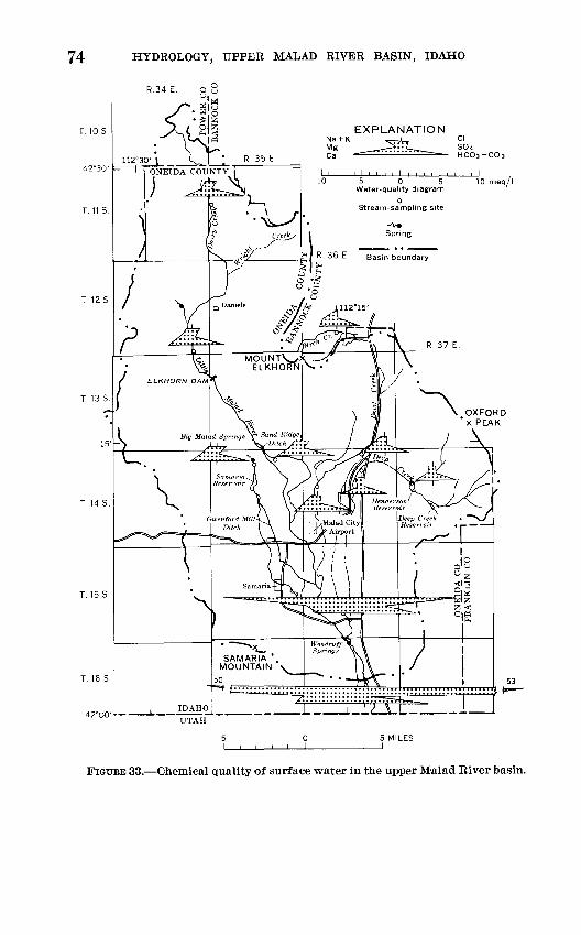
74 HYDROLOGY, UPPER MALAD RIVER BASIN, IDAHO
R.34E.
T. 10 S
T.11S
EXPLANATIONNa + K , 1 Cl
so <Ca HCOa+COs
10 meq/l
T 12 S
T 13 S
T 14 S
T.15 S
T. 16 S
42"00 f L '
FIGURE 33. Chemical quality of surface water in the upper M'alad Biver basin.
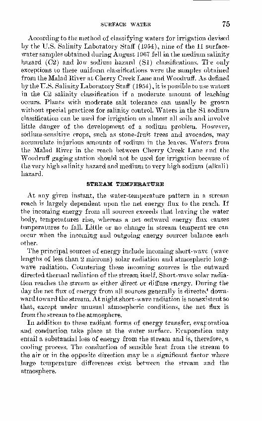
SURFACE WATER 75
According to the method of classifying waters for irrigation devised by the U.S. Salinity Laboratory Staff (1954), nine of the 11 surface- water samples obtained during August 1967 fell in the medium salinity hazard (C2) and low sodium hazard (Si) classifications. TTe only exceptions to these uniform classifications were the samples obtained from the Malad River at Cherry Creek Lane and Woodruff. As denned by the U.S. Salinity Laboratory Staff (1954), it is possible to use waters in the C2 salinity classification if a moderate amount of leaching occurs. Plants with moderate salt tolerance can usually be grown without special practices for salinity control. Waters in the SI sodium classification can be used for irrigation on almost all soils and involve little danger of the development of a sodium problem. However, sodium-sensitive crops, such as stone-fruit trees and avocados, may accumulate injurious amounts of sodium in the leaves. Waters from the Malad River in the reach between Cherry Creek Lane ?nd the Woodruff gaging station should not be used for irrigation because of the very high salinity hazard and medium to very high sodium (alkali) hazard.
STREAM TEMPERATURE
At any given instant, the water-temperature pattern in a stream reach is largely dependent upon the net energy flux to the reach. If the incoming energy from all sources exceeds that leaving the water body, temperatures rise, whereas a net outward energy flux causes temperatures to fall. Little or no change in stream temperature can occur when the incoming and outgoing energy sources balance each other.
The principal sources of energy include incoming short-wave (wave lengths of less than 2 microns) solar radiation and atmospheric long wave radiation. Countering these incoming sources is the outward directed thermal radiation of the stream itself. Short-wave solar radia tion reaches the stream as either direct or diffuse energy. During the day the net flux of energy from all sources generally is directed down ward toward the stream. At night short-wave radiation is nonexistent so that, except under unusual atmospheric conditions, the net flux is from the stream to the atmosphere.
In addition to these radiant forms of energy transfer, evaporation and conduction take place at the water surface. Evaporation may entail a substantial loss of energy from the stream and is, therefore, a cooling process. The conduction of sensible heat from the stream to the air or in the opposite direction may be a significant factor where large temperature differences exist between the stream and the atmosphere.
76 HYDROLOGY, UPPER MALAD RIVER BASEST, IDAHO
111 general, the above factors are of paramount importance with regard to water temperatures; other energy sinks and sources are usually negligible. Local geologic, topographic, or hydrologic con ditions, however, may create unusual thermal imbalances that exert considerable control on temperature. For example, the seasonal fluc tuation of water temperature of two streams on Long Island was found to be considerably less along reaches receiving heavy ground- water inflow than in reaches where such inflow was of lesser magnitude. (Pluhowski, 1961, p. D55-D58). The advection of a disproportionate quantity of energy from the ground-water reservoir was the dominant factor controlling the temperatures in the middle reaches of the streams. Moore (1964, p. D185-D189) found that stream temperatures in Oregon in east-west oriented streams are 2° to 4°C warmer in July than temperatures in north-south oriented streams. This is due to the fact that east-west oriented streams receive 5 to 20 percent more solar radiation than do north-south trending rivers (Geiger, 19C5, p. 202). Clearly, the temperature regimen of any stream reach is a function of many complex interrelated parameters.
Thermal patterns in the basin were determined by a series of tem perature observations made in three watercourses on August 15, 1966 (fig. 34). Sky conditions were clear throughout much of the day; only a few high scattered cirrus clouds were observed during the afternoon. Both the level of atmospheric haze and the percentage of relative humidity were low so that ineteorologic factors produced nearly ideal conditions for the transfer of large amounts of solar energy. Air temperatures were 43 degrees to 94 degrees F, for a range of 51 degrees F a large daily fluctuation even for the semiarid Malad Valley.
Water temperatures at the source of the Malad River below Big Malad Springs fluctuated little despite the strong downward flux of radiant energy. The measurement site at this point was at the outlet of a small pond created by gravity springs. It is likely that the temperature of the spring water entering the pond was constant throughout the day. Therefore, the small temperature fluctuation observed at the outlet of the pond was due to energy exchanged at its surface.
Water temperatures fluctuated nearly 17° C during the day in the Malad River near Cherry Creek, a point about 12 miles below the source. The discharge at this site was less than 0.5 cfc, owing to upstream diversions and natural channel losses. Sluggish flow com bined with a high ratio of water surface area to volume produced the large observed temperature fluctuation. Stream temperatures at this site reached a maximum about 2 hours earlier than air tempera ture. Owing to the north-south orientation of the Malad River at
SURFACE WATER 77
St. Johns Canal near Malad City
Malad River below Big Malad Spring
12p.m.
FIGURE 34. Air and stream temperatures on Aug. 15, 1966, at selected sitesin the Malad Valley.
Cherry Creek Lane and to 10-foot-high banks, considerable shading overspread the stream by midafternoon. With the ensuing reduction of solar energy, there was a reversal in net energy flux, causing water temperatures to fall earlier than expected.
During the irrigation season the entire flow of the Little Malad River is diverted into St. Johns Canal. Accordingly, thermal patterns in the canal are representative of those in the Little Malad Eiver. Water temperatures in the canal fluctuated between the temp «,rature ranges previously discussed; the observed range was less than 6° C. The discharge (about 10 cfs) and the depth-width ratio were sub stantially greater in the canal than at either of the other sites where temperature was measured. As a consequence, the low ratio of water surface area to volume in the canal attenuated temperature variations. Highest temperatures in the canal occurred after the time of maximum air temperature owing to a slow rate of energy release which resulted from the relatively large quantity of stored heat in the water.
78 HYDROLOGY, UPPER MALAD RIVER BASIN, IDAHO
GBAIN-SIZE DISTBIBUTION IN STBEAM CHANNELS
In general, the rate at which streambed particles decrease in size in the downstream direction is relatively rapid in the upstream reaches of streams (Leopold and others, 1964, p. 191). Even a cursory examination of streambed material will corroborate the validity of this statement along most reaches in the project arer. Angular boulders are common in high-altitude ephemeral washes; well- rounded boulders and cobbles may be found in the upper reaches of perennial streams; and fine gravel, silt, and clay predominate in the do\vnstream reaches of virtually all major watercourses in the basin.
Two streams, the Little Malad River and Devil Creek, were selected for field analysis to obtain quantitative data on streambed material. The pebble-count method was used. At each site 100 pebbles were col lected at random from the streambed. Measurements of the three principal axes of each pebble were made, and the pebbles were ranked according to size (minimum 2 mm). The number of pebbles in each size category was determined. The resulting totals were then cumulated from the smallest to the largest category and plotted on semilogarithmic paper to analyze particle sizes in each selected reach.
The largest particles in the streambed of Devil Creek were found in an ephemeral wash below the point where the stream f rst has an identifiable channel. The D50 (the diameter exceeded by 50 percent of the grains) point is about TO mm (fig. 35). A sharp reduction in grain sizes was observed near the former stream-gaging station above Campbell Creek and in the reach above Evans dividers. These sites are 5 and 8.5 miles, respectively, below the upstream ephemeral sampling point. The D50 grain size is about 10 mm at both sides; however, fewer large particles were found in the reach above Evans dividers. Thus, grain sizes decrease rapidly in the uppermost reaches of Devil Creek but much more slowly farther downstream.
The same general pattern of decreasing grain sizes in the down stream direction is exhibited in the channel of the Little Malad River (fig. 35). The sampling site in sec. 26, T. 12 S., R. 34 E., is about half a mile below the point where the combined flow of Dairy Creek and Wright Creek enters the river. The D50 grain size at thir station is about 90 mm, whereas it is 60 mm just below Elkhorn Dam, 4 miles downstream. A sample of the bed material from Dairy Creek (fig. 35) had grain sizes considerably smaller than those measured at either site on the Little Malad River. The bulk of the coarse material in the Little Malad River, therefore, must be derived from Wright Creek, whose channel contains numerous boulders and cobbles.
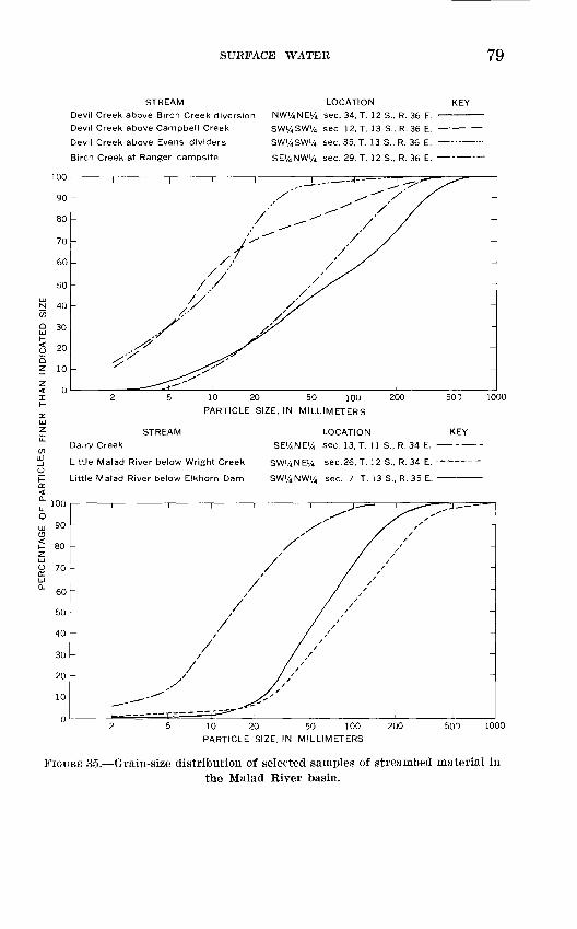
SURFACE WATER 79
STREAM
Devil Creek above Birch Creek diversion
Devil Creek above Campbell Creek
Devil Creek above Evans dividers
Birch Creek at Ranger campsite
LOCATION KEY NWi/4 NEi/4 sec. 34, T. 12 S., R. 36 E.
swi/4 swi/4 sec 12, T. 13 s., R.se E. SWViSWVi sec. 35, T. 13 S., R. 36 E. -
SEViNWVi sec. 29, T. 12 S., R. 36 E. -
100
10 20 50 100
PARTICLE SIZE, IN MILLIMETERS
200 500 1000
STREAM
Dairy Creek
Little Malad River below Wright Creek
Little Malad River below Elkhorn Dam
LOCATION KEY
S£1/4NEi/4 sec. 13, T. 11 S., R. 34 E. - -
SWViNEVi sec.26, T. 12 S., R. 34 E. -
SWi/4 NWi/4 sec. 7. T. 13 S., R. 35 E.
10 20 50 100 PARTICLE SIZE, IN MILLIMETERS
200 500 1000
FIGURE 35. Grain-size distribution of selected samples of streambed material inthe Malad River basin.
80 HYDROLOGY, UPPER MALAD RIVER BASIN, IDAHO
WATER MANAGEMENT
The quantity of Avater available for irrigation in the upper Malad River basin is far short of that required to supply all suitable agricul tural lands. A principal objective of water management is to distribute the available Avater so that optimum beneficial use may be derived from the existing supply. Such factors as Avater rights, definitions of maximum beneficial use, and conflicting economic and political in terests often complicate the task of making a Avater-rranagement study and of carrying out technical recommendations. Water problems involving surface supplies are generally apparent and the law may be applied to settle litigation. Serious misuse of surface-water supplies is usually avoided because users and managers are instinctively aware of the more obvious instances of nonbeneficial practices. Unfortu nately, the situation with regard to ground-Avater management is not so readily apparent. The response of aquifers to pumping is relatively sloAv, so the effects of stresses on the ground-Avater system cannot be predicted with any great degree of precision.
Ideally, efficient basimvide water management generally implies the conjunctive use of ground-Avater and surf ace-Avater resources. This can be achieved because aquifers are basically nonstructural storage reser voirs and are therefore analogous to surface reservoirs. Accordingly, systems-analysis techniques such as linear and dynamic programming can be used to suggest optimal operating procedures and to evaluate maximum accrued benefits within an existing framework of economic, legal, and physical constraints.
The ground-water reservoir underlying the Malad Valley may seem to contain an inexhaustible supply of potable Avater. In fact the aquifer system does contain a large supply of stored Avater, but its quality ranges widely from very poor to excellent. Although the reserve of fresh ground water has been adequate to meet most demands, the sup ply can be seriously depleted by excessive pumpage which leads to increased pumping costs, deterioration of water quality, and reduced yields from Avells. Data currently available are not adequate to deter mine what is excessive. Wells must produce a cone of depression in the water table or lower artesian heads if they are to yield water. Lower ing of water levels within an aquifer system is essential if its potential is to be achieved. A major objective of ground-Avater management is to determine an aquifer's limitations and to operate Avithin those con straints. Continued decline of \vater levels during periods of normal or above-normal recharge may be a danger signal. As shown in figure 21, pressure heads and Avater levels have been declining for many years in parts of the Malad Valley. No doubt drought and deficiert recharge intensified this trend, but it is unlikely that drought was the sole cause of the decline.
WATER MANAGEMENT 81
To gain an understanding of the internal state of the aquifer system, one must (1) define the principal hydrogeologic controls, (2) deter mine the subsurface boundaries of the ground-water reservoir, (3) evaluate the spatial distribution of transmissivity and storage co efficients, and (4) assess the quality of the water within the system. Little information is currently available in the upper Malad River basin regarding any of these important ground-water considerations. Clearly, the current program of water-level observations should be continued. Moreover, an expanded program of ground-water investi gation must be instituted to provide data needed for the assessment of the basin's ground-water resources.
As noted elsewhere, surface-water users in the basin generally are proficient in managing their small water supplies. However, attempts to store part of the excess water generated by spring freshets for use during the irrigation season have been only partially successful. Hen- derson Reservoir and Deep Creek Reservoir on Deep Creek are usually filled following the normally heavy late winter and early spring runoff, and the bulk of this water is used for irrigation. Elkhorn Reser voir on the Little Malad River failed from the start to held any appreciable amount of water, owing to large bank and underflow losses. Samaria Reservoir on the Malad River is much less dependent on spring runoff because it receives a steady supply from springs and seeps. Only small diversion dams have been built on Devil Creek, although several suitable sites for larger dams are available. Owing to the generally poor quality of the streamflow at the Woodruff gage, especially during low-flow periods, it is doubtful that this water can be stored for downvalley irrigation without first diluting it with fresh water.
Eradication of phreatic growths, efficient irrigation practices, and salvaging water lost by evapotranspiration are perhaps th<^ most promising approaches for increasing the efficiency of water use in the basin. By first lowering water levels 30 to 50 feet in areas where ground water is lost by evapotranspiration and then maintaining these levels, it should be possible to salvage part of the natural discharge from the ground-water reservoir. However, as water levels decline, some loss of streamflow may occur, especially in reaches that normally receive part of their flow from ground-water seepage. Ground-water discharge by evapotranspiration is widespread in parts of the lower Malad Valley. In these areas the soils consist of fine-grained mater: al that is saturated with precipitated salts. The poorly drained tight soils are not conducive to leaching, so it is doubtful whether such land could be of economic value for agriculture. In other parts of thQ, basin, it should be economically feasible to combine ground-water roclama-

82 HYDROLOGY, UPPER MALAD RIVER BASIN, IDAHO
tion projects with programs designed to remove low-benefit phreatic vegetation. Decreasing evapotranspiration loss in areas of phreato- phytes while depleting streamflow within allowable limits would increase the beneficial use of water in the basin by an amount equiva lent to the water salvaged.
Although State law prohibits waste of water from artesian wells (McGuinness, 1951, p. 19), many flowing wells in the lower Malad Valley remain uncapped throughout the year. Some water users main tain, however, that the winter flow is not wasted. In their opinion, this flow is necessary to flush salts from the fields. Nevertheless, leaky or uncased artesian wells are numerous and these contribute to reductions of pressure and storage and to the basin's overall water loss. Much of the water from uncapped artesian wells is applied continually to large tracts of land that are now waterlogged. Repairing poorly con structed and leaky artesian wells would be a useful step in curtailing the inefficient use of ground water.
SUMMARY AND CONCLUSIONS
A thick sequence of interbedded clay, silt, sand, and gravel deposits of highly variable horizontal and vertical permeability constitutes the ground-water reservoir underlying the Malad Valley. The thickness of this unconsolidated material is greater than 700 feet locally; its total thickness is not known. The project area has extensive reserves of stored ground water which have fostered irrigation in the valley, especially south of the latitude of Malad City where arteHan condi tions are prevalent. Since the end of World War II, increased pumpage and protracted drought have steadily lowered artesian pressure heads in many parts of the lower Malad Valley. Runoff from the hard-rock mountainous areas around the periphery of the basin is one of the main sources of recharge to the ground-water reservoir. Th°s principal direction of grbund-water movement is southward in the Malad Valley (figure 3) and generally parallel to the longitudinal axes of the prin cipal tributary valleys. Discharge from the ground-water system is by evapotranspiration, springs, seepage to streams, pumping, and as underflow past the constricted lower Malad Valley.
The orientation of the mountain ranges east and west of the study area orthogonally to the prevailing eastward flow of air creates an environment that is very efficient in removing atmospheric moisture. Runoff from the high elevations of the basin is from eight to nearly 20 times greater than that generated in low-lying areas.
The principal climatic controls are the large-scale surface and upper-air centers of atmospheric action that govern the flow of mois ture to the basin. Owing to its inland position and the numerous

SUMMARY AND CONCLUSIONS 83
meridional mountain ranges to the west, a minimum uplift of 6,000 feet is applied to airmasses moving over the basin from the Pacific Ocean. Consequently, the precipitable water of originally moist air- masses is largely depleted long before the airmasses reach the Malad River basin. In addition, migratory low-pressure systems are often diverted away from the project area by high pressure that normally develops in the atmosphere over the Great Basin. The characteristic sinking motion of the air in high-pressure systems tends to further desiccate the atmosphere. This combination of factors is largely responsible for the semiarid climate of the Malad basin.
Ephemeral streams are common to much of the basin, particularly in the mountains and the lower Malad Valley. Stream channels are well defined in the uplands; however, most of them rapidly become indistinct after moving onto the alluvial fans that surround the Malad Valley. The principal streams of the basin are perennial, except below reaches where the entire flow is diverted into canals for irriga tion or in the lower Malad Valley where seepage losses may reduce flows to zero. Perennial streams are supplied by gravity springs that characteristically discharge fairly uniform quantities of water.
Streamflow records in the basin were first collected in 1911; however, a continuing stream-gaging program did not begin until 1931. Low- flow and flood analyses were prepared for several long-term stations covering a 29-year base period, water years 1932-60. Well-sustained low flows characterize the upper reaches of most perennial streams, but greater discharge variability and therefore less reliability are common in the lower reaches. A regional flood-frequency analysis of the basin shows that at the 50-year recurrence interval, peak in stantaneous runoff values of 16.5 cfs per sq mi may be expected from drainage areas of 20 sq mi; 11 cfs per sq mi from drainage areas of 50 sq mi; and 8.5 cfs per sq mi from drainage areas of 100 sq mi.
As in many other parts of the Nation, storage of surface-water resources by the construction of dams and reservoirs is limited in the Malad River basin owing to a scarcity of suitable sites. Two streams, Devil Creek and the Little Malad River, may be suitable for limited water development. A moderate supply of water is available in both streams, particularly if some storage is provided.
Stream temperatures are a function of many interrelated variables, so water-temperature fluctuations may differ considerably from point to point along a stream. The range of water temperatures on a clear summer day was observed to be 1°C at a point near the source of the Malad River to almost 17 °C in a reach 12 miles downstream. Spring flow at the source kept stream temperatures within a very narrow range, whereas a high ratio of water surface area to volume at the

84 HYDROLOGY, UPPER MALAD RIVER BASIN, IDAFO
downstream site permitted high solar-radiation absorptior to produce the large observed fluctuation.
The grain size of streambed material in Devil Creek decreases rapidly below the headwaters of the stream. The D50 size (the diam eter exceeded by 50 percent of the grains) at the source is 70 mm, whereas at a point 5 miles downstream it is only 10 mm. The bulk of the coarse material in the Little Malad River is derived from Wright Creek rather than Dairy Creek, which has a preponderance of relatively fine-grained bed material. There is a gradual downstream siae reduction in streambed material in. both the Little Malad River and in the middle and lower reaches of Devil Creek.
The computed mean annual water yield of the project area is about 115,000 acre-feet per year, which is equivalent to 4.0 inches over the basin. The mean annual outflow from the basin is computed to be 51,000 acre-feet of surface water and 28,000 acre-feet of ground water. The difference between input and output is largely accounted for by evapotranspiration losses, especially from irrigated areas. Mower and Nace (1957) have estimated losses from phreatic growths at 37,000 acre-feet. Accordingly, decreasing evapotranspiration in ar?.as infested by phreatophytes could substantially increase the beneficial use of water in the basin. Efficient use of the water resources of the basin would be of direct benefit to agriculture, as thousands of acr^s of fertile land could be brought under irrigation by salvaging this water.
REFERENCES CITED
Bradley, F. H., 1873, Report of Frank H. Bradley, geologist of the Snake Riverdivision, in Hayden, F. V., U.S. Geol. and Geog. Survey of the Terr., Ann.Rept. 6, 1872: p. 189-271.
Brown, M. J., 1959, The relation of weather factors to the yield of winter wheatin Box Elder County, Utah: Monthly Weather Rev. v. 87, no. 3, p. 99.
Butler, E. B., Reid, J. K., and Berwick, V. K., 1966, Magnitude and frequency offloods in the United States Part 10, The Great Basin: U.S. Geol. SurveyWater-Supply Paper 1684, 256 p.
Dalrymple, Tate, 1960, Flood-frequency analysis: U.S. Geol. Survey Water-Supply Paper 1543-A, 80 p.
Fenneman, N. M., 1931, Physiography of western United States: New York, Mc-Graw-Hill Book Co., 510 p.
Geiger, Rudolf, 1965, The climate near the ground: Cambridge, Mass., HarvardUniv. Press, 611 p.
Gumbel, E. J., 1945, Floods estimated by the probability method: Enj*. News-Rec.,June 14, p. 97-101.
Hadley, R. F., 1963, Hydrology of stock-water development in southeasternIdaho: U.S. Geol. Survey Water-Supply Paper 1475-P, p. 563-5P9.
Howell, G. F., 1960, Early history of the Malad Valley: Brigham Young Univ.master's thesis, 110 p.
Klein, W. H., 1956, Some empirical characteristics of long waves on monthly meancharts : Monthly Weather Rev., v. 80, no. 11, p. 203-219.
REFERENCES CITED 85
Landsberg, Helmut, 1958, Physical climatology: Du Bois, Pa., Gray PublishingCo., Inc., 446 p.
Langbein, W. B., and others, 1949, Annual runoff in the United States: U.S. Geol.Survey Circ. 52,14 p.
Leopold, L. B., Wolman, G. M., and Miller, J. P., 1964, Fluvial processes in geo-morphology : San Francisco, Calif, W. H. Freeman Co., 522 p.
Livingston, Penn, and McDonald, H. R., 1943, Underground leakage from artesianwells in Malad Valley, Idaho : U.S. Geol. Survey open-file rept., 38 p., 4 pis.
McGuinness, C. L., 1951, Water law with special reference to ground water: U.S.Geol. Survey Circ. 117, 30 p.
Meyer, A. F, 1944, The elements of hydrology: New York, John Wiley ard Sons,Inc, 522 p.
Moore, A. M., 1964, Correlation and analysis of water-temperature data for Ore gon streams, in Geological Survey research 1964: U.S. Geol. Survey Prof.Paper 501-D, p. D185-D189.
Mower, R. W., and Nace, R. L., 1957, Water consumption by water-loving plants inthe Malad Valley, Oneida County, Idaho: U.S. Geol. Survey Water-SupplyPaper 1412, 33 p.
Xace, R. L., and others, 1961, Water resources of the Raft River basin, Idaho- Utah : U.S. Geol. Survey Water-Supply Paper 1587,138 p.
Peale, A. C., 1879, Report on the geology of the Green River district [Wyoming],in Hayden, F. V., U.S. Geol. and Geog. Survey of the Terr., Ann. Rept. 11,1877 :p. 509-S46.
Piper, A. M., 1924, Possibility of petroleum in Power and Oneida Counties, Idaho :Idaho Bur. Mines and Geology, Pamph. 12, 24 p.
Pluhowski, E. J., 1961, Variation in temperature of two streams on Long Island,New York, in Short papers in the geologic and hydrologic sciences: U.S. GeoLSurvey Professional Paper 424-D, p. D55-D58.
Pluhowski, E. J., and Kantrowitz, I. H., 1964, Hydrology of the Babylon-Is'ip area,Suffolk County, Long Island, New York. U.S. Geol. Survey Water-SupplyPaper 1768, 119 p.
Powell, R. W., 1943, A simple method of estimating flood frequencies: Civil Eng.,v. 13, no. 2, p. 105-106.
Thomas, C. A., and Lamke, R. D., 1962, Floods of February 1962 in southern Idahoand northeastern Nevada: U.S. Geol. Survey Circ. 467, 30 p.
Thompson, D. G., and Faris, R. W., 1932, Preliminary report of water resourcesof Malad and Curlew Valleys, Oneida County, Idaho: U.S. Geol. Surveyopen-file rept., 140 p.
Thornthwaite, C. W., 1948, An approach toward a rational classification of cli mate : Geog. Rev., v. 38, p. 55-94.
U.S. Department of Commerce, 1953, Critical meteorological conditions fo" designfloods in the Snake River basin: Weather Bur. Coop. Rept. 11, p. 11.
1961, Rainfall frequency atlas of the United States: Weather Bur. Tech.Paper 40,115 p.
U.S. Salinity Laboratory Staff, 1954, Diagnosis and improvement of saline andalkali soils: U.S. Dept. Agriculture Handb. 60,160 p.
Van Hylckama, T. E. A., 1959, A monogram to determine monthly potential evap-otranspiration : Monthly Weather Rev., v. 87, no. 3, p. 107.
Williams, G. R., and others, 1940, Natural water loss in selected drainage basins:U.S. Geol. Survey Water-Supply Paper 846, 62 p.
INDEX
[Italic page numbers indicate major references]
A Page Agriculture ...................... _ ..... 9
development. 10length of growing seascn--_-_._-_._ ......_ 14
Alfalfa _-.--_ ._..----. .- _-_- 11,32Alkali-.....-...-...-.......-.- ......... 3Alluvial fans Altitude, Malad Valley. Aquicludes- ............Aquifers---------------
7.----___._ 7.... .-. ..... 39------.-..----- 39
artesian. ------._-..-------.----_-. 2,3,10,44water-table- . . ....--.-.-.-...-.-.-.... 44
Artesian ground water-..-. ______ ........... 39Artesian wells ------------------.-.------.-- 3,82Aspen. .. ...... ... ...... ..----- ------. .- 11Atmosphere, circulation patterns. -..-.-.- 12Avocados- -.----------------_-_----_-_-_ -__ 75
Bannock County. _ -_- 3BannockRange. -__..---.----.--.-_-_-._. _3,7,38 Barley..--.. --- ----. ---- ..--- 10Basin and Range physiographic province..... 7Bear River.-.._._._.. .....--._......-...-. 9Big Malad Springs--...... ..-.- 76Birch Creek...-.---------.-....---- 10,38,43,49,72Birch Creek near Downey, gaging station. _. -. SB Blue Spring Hills---..-------------------- 3,7,38Bonneville shoreline. -._._. ___.___ 38
Campbell Creek... .-.-. ---.-..-.. 38,50,78C apillary water....-.-................. -.-.. 48Caribou Range................... ..... ... 27Cattails---------------------------------- 11Cattle-----.-------------.------. ----- 10Cherry Creek.... ........... ...... ... 43Cherry Creek Lane_........................ 45Circulation patterns. 18,20Climate, Aleutian low..- - .- -------- 11
analysis of records. - . - 27controls---- --------------------- 11,27,82eastern Pacific high................... .. 12Great Basin high..__............ .... . 11
Crops-.-------------------------------- 10
D
Dairy Creek...-._.__-..___.------...-- 78,84Daniels ---------------------------------- 10Davis Creek, reservoir. ..................... 1CDeep Creek--. 7,48,51,53,72,81Deep Creek below First Creek, near Malad
City, gaging station SB
Page Deep Creek Reservoir. 10,81Desert saltgrass. -- _ 11Devil Creek.----------. _. 7,10,38, 50, 5',81,83,84
reservoir potential.__-- 64Devil Creek above Campbell Creek, near
Malad City, gaging station.----- 51,55,58,60,64
Devil Creek above Evans dividers, nearMalad City, gaging station....... 66
Discharge, artesian wells.------------------ 3Devil Creek-....---...-.-------- 61Malad River at Cherry Creek Lane------ 45Malad River at Woodruff- --__-__--- 45,65
Dissolved-solids content, surface water. ------ 72Drought -- n
E
Elkhorn Reservoir (Dam) .....--.. . 10,38,78,81unsatisfactory............................ 53
Ephemeral streams. 7,83Equation, recurrence interval . 68
underflow 49water loss. - __ - - 31water yield..... -------------------------- 32
Evans dividers.-----..---------------------.- 56,78Evaporation . _ --- - .- 30,32Evapo transpiration. .--_---_._--- 16, SI, 45,49
definition . 31Long Island, N.Y-.......----_--. -_-_- 34losses.. ------------ 4potential---_ - - 34, 50Thornthwaite's method. - ____-_ 32, 50Williams plot ..... -------------- 35
Faults -- - - - - 3,33,39,45Fir. 11Floods BB
magnitude determination .... .....--. 71Malad Valley-- 66
Flow-duration curves, surface water.._._. __ 58Flowing wells, Malad City. - - - - 10Forage crops 10Franklin County-. - 3
GGaging stations:
Birch Creek near Downey 55Deep Creek below First Creek, near
MaladCity ------------------ 55Devil Creek above Campbell Creek, near
Malad City.. -------- 51,55,58,60,64
88 INDEX
Gaging stations Continued Page Devil Creek above Evans dividers, near
Malad City.-..----.-_...-._----- 56Little Malad River above Elkhorn Reser
voir (Dam), near Malad City-... 51,56 Malad River at Cherry Creek Lane. - _ _. _ 72 Malad River ar Woodruff. ---___..___.... 45,
49, 50,51, 56, 65,72,75,81 Malad River below springs, near Malad
City --....--.....-_...__.-..... 56Portneuf River at Topaz Station. -.-.-___ 35 Willow Creek near Ririe ............... 35
Geography.-.---. -___._-.____..____...___.___ 6Grain-size analysis, streams_. -_......______ 78Gravity springs.............................. 76,83Greasewood- -___ .____.________.______ _ _ 11Great Basin............................ 14,22,70,83Great Salt Lake..-........................... 9Ground water, artesian..--.....----....-....- 39
discharge...-------....................... 45,82
infiltration galleries..-......--.......---.- 48management- -.-....--.....--........-.-- 10movement__ ____________________________ 44, 82nonartesian............................... 10pumping.-.-......--..._.--......-.._..-. 22recharge--.......-...---....---.-....--.-- 41reservoir ....................... 2,39,65,80,82underflow.-.........-_-_....-._.....-. 44,48,49
HHardness, surface water. Hay....................
................ 72
.--.---.___---.. 10Henderson Reservoir................ 38,51,53,72,81Hydrology, quantitative........---.-..-.--.. %7Hydrometeorology........................... 18
Introduction- ................................ %Investigations, previous.-.................... 3Irrigation--..... _------..-_-----_-_-.-.--._-_ 2,9
Juniper-
Lake Bonneville-............................. 38Lake Bonneville Group...-..__.......- -__ 38,39Land pans, class A.--_._ _____ -_.__ _-__ 30Langbein's method, water yield-............. 32, 50Lapse rate-.------__...-..... .....- ... 16,66Limestone formations, Blue Spring Hills- - - - - 3Little Malad River............. 7,47,51,77,81,83,84
reservoir_.............................. 10potential............................. 64
Little Malad River above Elkhorn Reservoir (Dam), near Malad City, gaging station-.......................... 51,66
Location and extent of area................... 3Long Island, N.Y., evapotranspiration.------ 34
stream temperatures. -............... _ 76Low-flow characteristics, streams...-......--. 53
M
Madison Limestone-
Page Malad City............. 2,3,6,10, 14,22,38,39,41,82
precipitation...__................... 20,24,66water supply............................. 48
Malad City Airport, precipitation............ 66temperature.-............................ 14
Malad Range...-_.......................... 3,7,38Malad River, drainage area...---_........... 3
reservoir-_....._...................... 81source.................................... 7temperature.............................. 76
Malad River at Cherry Creek Lane, gagingstation........................... 72
Malad River at Woodruff, gaging station..... 45,49,50, 51, 56, 65, 72,75,81
Malad River below springs, near Malad City,gaging station...__________.___.__ 56
Malad Valley..------_.-_--..--.-.-.-. 3,32,39,76acreage irrigated-...--....--.---.......... 50
alluvial fans-..._........................... 43flood of 1962.............................. 66ground-water reservoir.----- -_._-- - 65,80population............................... 6topography and drainage................. 7
Marsh reedgrass----------.......--.....-.... 11Moisture barriers.----_.----_-----_---.- ---- 12,24Monroe Canyon Limestone------.-------.-.- 38Mount Elkhorn-.__-__....-. .......-..-.. 7Mower, R. W., written communication ._ 38
O Ogden, Utah............ ................... 6Oneida County__........-..---...-..-..-.. 3,6Oregon, stream temperatures. --....... ..--- 76Oxford Peak................................ 7
Perched water..... Perennial streams. Phreatophytes- - - - Pickleweed----.-.. Fine -------
.....-.........- . 39
. ___.-. _ 83 ...-....-...--- ... 11.-----.-.-----.-...... 11.---.._ -.-.. - 11
Pleasantview.-.............................. 7,41Pocatello-------------------------------- 3,20,24Population, Malad Valley.........._------ 6Portneuf River at Topaz Statton, gaging
station----.----...-------.-----. 35Potatoes ...... .......................... 10Power County.. ........................... 3Precipitation, areal distribution_........... &7
eflective....................--- ..------. 50intensity-................................ #4Malad City.---..-..-.---.-------.--. 20,24,66Malad City Airport-.--...,-------------- 66mean annual....-..--.---------------..-. 30,38relation to altitude-.-----.-------. -- - 28seasonal distribution.---...............-- $4
Provo shoreline ........-....-.----..-.-.-.- 38Pumping, ground water------.------.-------- 22Purpose of report-..........-.....--.....-.--- 3
R11Rabbitbrush-...---. -.--.................
Rainfall. See Precipitation.Recurrence interval, formula................. 68Relief, Malad Valley___....._........... 7
INDEX 89
Page Reservoirs..................... 10,38,51,53,64,72,81Rocky Mountains...--....-...-.-..---....-.. 18Rushes....................................... 11
Sagebrush..........St. Johns Canal..-. Salinization of soils- Salt-...............Salt Lake City, Utah......................... 3,(Salt Lake Fonnation- Samaria Reservoir....Scrub maple...__... Scrub oak............Sedge -..-----....
_......-..-....... 38.................. 81.................. 11.................. 11................... 11
Sheep..-..........-.-.-..-..-.----------.--.. 10Snake River basin............................ 10Soda Springs. ............................. 6Springs. ........................... 7,45,76,82,83Spruce _. _.. - . 11Stone-fruit trees...-..-.-.--.-.---.-_------... 75Streams. See Surface water.Sugar beets................................... 10,32Summary and conclusions -----_.-.-----_. 8iSurface water.. ........................... 61
days of deficient discharge................ 61dissolved-solids content .---.--.-----_.- 72droughts.-...-...--.-.-..----------.--.-_ 22ephemeral streams-. .................. 7,83floods.-----.....-.........-.......-.. .. 65flow-duration curves.-------- . - 58frequency-mass curves_.........-.. .. 62grain-size distribution--.-. . _ - 78hardness-.------.-,-..---.------.-- 72low-flow characteristics.. ..-.----------. 55low-flow frequency curves.-.._____- _. 60management- ___.._.____.____.__ _. ___ 10monthly discharge summary.-.......,._. 55perennial streams .....----..- -.-..--. 83quality. ----___ ---. --.- -- -- 71salinity hazard--.....------ .- - -- 75
---------- 48,83
Surface water Continued Page sodium hazard. --... ................... 75storage-required frequency. ........... 6ttemperature. ............................. 76,S3
Temperature, air...... ---. ... ....... 14water....--.----.-----------------.-- 75,83
Thornthwaite's method, evapotranspiration. - 32,50 Thunderstorms. ___ __.-. - -- -- 24Topography and drainage.----.------------- 7
U Underflow.. . - --- - 44,48,49
Vegetation.-.-.... .- -- -. . 11
W Warm Springs Canal.... - --- . ..... 50Wasatch Mountains...._ _ _ _ 27Water loss, estimates....-- .. ..--..-. --- 30,34
equation- ----...__ - - ----- 31Water management-_--_ . 80Water yield-.--..---.----------------- Si
above Woodruff--.....-....-..-..- ..-.- 51annual.................. .. --...--.... 50equation...... .............. .... ... 32evaluation. ---- - --.. --.--. 27Langbein's method....................... 32,50mean...........-..------------........... 35
Weather stations........----..- ..--.---.... 27Well-numbering system.._ __-_-_ __._-_ _ 5 Wells, artesian---.----------------- 3,82
flowing-................. .--..-....-.. 10Wells stratigraphic unit...--....---..------. 38Wheat..--... - .-- -- - 10,20 Willow Creek near Ririe, gaging station...... 35Wirerush- .- 11Woodruff.. -.--..-------------.-.- 3,7,30,35Woodruff fault.... -.- ----- 3,39,45Woodruff Springs....... ..-. . ...... 45,72Wright Creek-....----...-.-.. --- 9,78,84