1

BASIN SCALE CONCEPT VALIDATION: Urban Hydrology Model

Draft 09/13/12

By: Olivia Wright and Erkan Istanbulluoglu

Effective Impervious Area A rainfall-runoff depth analysis of storm events is used to estimate the effective impervious area

of the basin and the initial abstraction of impervious surfaces (Boyd et al. 1993, 1994). The

analysis evaluates the runoff depth of each storm as a function of the storm’s precipitation depth.

The slope of the relationship estimates the fraction of the basin that contributes to runoff, and the

rainfall axis intercept estimates the initial abstraction that must be satisfied before runoff can

occur.

Storm events were calculated by summing consecutively occurring hourly precipitation.

Individual storm events were separated by 24 hours of no precipitation. Due to the

responsiveness of our basin, we assumed the runoff event occurred during the same time period

as the precipitation event. Plotting the full range of observed storm events estimates an initial

abstraction as 4 mm. Runoff can be calculated as:

EIACIPR a )(

P is precipitation (hourly)

Ia is initial abstraction

C is runoff coefficient

EIA effective impervious fraction in basin

Figure 1 shows the rainfall-runoff depth plot for dry season storm events with initial abstraction

removed. The analysis focused on surface runoff with baseflow removed. The effective

impervious area during dry season storm events ranged from approximately 9-20%. For summer

rainfall, we assume that effective impervious area (EIA) is the dominant source of runoff and the

slope that captures the high end of storm event depths can be assumed to be EIA.

Figure 1. Rainfall- runoff depth plots

2

Table 1 presents the area of the impervious land use categories and the fraction of the basin they

cover. The total impervious area (TIA) calculated from spatial data is 70% of the basin, while the

estimated EIA is 20%.

Table 1. Impervious land cover area and fraction of basin

Hydrologic Modeling of land processes and LID treatment This study uses a lumped Urban Hydrology Model to estimate the long term hydrologic behavior

of Newaukum Urban basin considering current land cover [Istanbulluoglu et al., 2012], figure 2.

The model is a lumped representation of an urbanized landscape.

Figure 2. Conceptual representation of the processes in the Urban Hydrology Model

The depth averaged soil moisture in the root zone layer is calculated by the mass balance

equation (Istanbulluoglu, 2012)

)()( sDsETIdt

dsnZ aar

n is porosity

Zr is effective rooting depth

Impervious Category Area (acres) Fraction of Basin

Roads 41.32 0.15

Rooftop 24.92 0.09

Other 120.10 0.45

Total Impervious Area 186.34 0.70

Effective Impervious Area 53.46 0.20

3

s is soil moisture

t is time

Ia is infiltration rate

ETa is actual evapotranspiration rate

D is drainage

Interception from the canopy is calculated by:

),min( max ttI PVVIC

Imax is a maximum hourly interception

Vt is the fraction of vegetation cover on the land surface (includes dry and live

biomass)

P is depth of rainfall

When P is larger than CI, throughfall occurs at the same rate as precipitation. The precipitation

duration reaching the ground is reduced to account for initial filling of the canopy storage during

the early part of the rain event. When the soil is unsaturated, the infiltration rate is determined by

the minimum of the precipitation rate and the infiltration capacity. After soil saturation, the

infiltration rate is reduced to the drainage rate:

I

Ic

aCPs

CPs

D

IpI

1

10],min[

Ic is infiltration capacity

p is average pervious input rate

IMPfrac

CoeffEIAfracIMPfracCPCPp I

I

1

))()(()(

IMPfrac is the impervious surface fraction of the basin

EIAfrac is the effective impervious fraction of the basin

Coeff is the runoff coefficient

Surface runoff occurs when p exceeds Ia and is approximated by:

a

aa

sIp

IpIpR

0

)(

The root zone layer is assumed to have uniform soil texture, porosity, and hydraulic

conductivity. The drainage of the soil column by gravity is modeled to occur at the lowest

boundary of the soil layer. At soil saturation, the drainage is at its maximum and is calculated as

the saturated hydraulic conductivity (Ks) and decays exponentially to a value of zero at field

capacity, sfc.

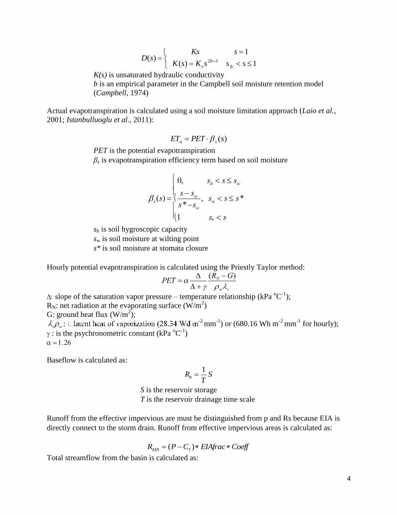
4

1)(

1)( 32

sssKsK

sKssD

fc

b

s

K(s) is unsaturated hydraulic conductivity

b is an empirical parameter in the Campbell soil moisture retention model

(Campbell, 1974)

Actual evapotranspiration is calculated using a soil moisture limitation approach (Laio et al.,

2001; Istanbulluoglu et al., 2011):

)(sPETET sa

PET is the potential evapotranspiration

βs is evapotranspiration efficiency term based on soil moisture

s(s)

0, sh s sw

s sw

s*sw, sw s s*

1 s* s

sh is soil hygroscopic capacity

sw is soil moisture at wilting point

s* is soil moisture at stomata closure

Hourly potential evapotranspiration is calculated using the Priestly Taylor method:

PET

(RN G)

wv slope of the saturation vapor pressure – temperature relationship (kPa

oC

-1);

RN: net radiation at the evaporating surface (W/m2)

G: ground heat flux (W/m2);

vw-2

mm-1

) or (680.16 Wh m-2

mm-1

for hourly);

: is the psychronometric constant (kPa oC

-1)

Baseflow is calculated as:

ST

Rb

1

S is the reservoir storage

T is the reservoir drainage time scale

Runoff from the effective impervious are must be distinguished from p and Rs because EIA is

directly connect to the storm drain. Runoff from effective impervious areas is calculated as:

CoeffEIAfracCPR IEIA )( Total streamflow from the basin is calculated as:

5

EIAsb RRRR

The model also includes a dynamic vegetation component that updates the amount of biomass

and LAI below and above ground [Istanbulluoglu et al., 2012].

Model Variations and Decision variables Three variations of the model are evaluated to determine the effectiveness of BMP application:

(1) Urban land use (no BMPs), (2) Urban land use with BMP treatment and (3) forested

conditions.

The urban land use model with no BMP treatment simulates existing hydrologic conditions to

evaluate the current health of the catchment. The urban land use with BMP treatment model

simulates the impact various BMP treatment scenarios have on basin hydrology. The forested

model simulates the hydrology of the basin with a natural landscape prior to development. The

forested condition is used to further evaluate the effectiveness of the BMP scenario model.

Model input and calibration The model is forced with precipitation and potential evapotranspiration. Input to the model

includes the basin’s total impervious fraction, effective impervious fraction, and runoff

coefficient.

Total Impervious Fraction 0.70

Effective Impervious Fraction 0.20

Coefficient 0.90

Table 2. Model basin characteristic input values

The urban land use (no BMPs) modele is calibrated to 3 years of observed streamflow data. The

calibration parameters of the model are Fg, Variable Infiltration Capacity (VIC) b-shape

parameter, and T. Fg controls the fraction of drainage water that directly contributes to

groundwater, VIC b-shape parameter controls the shape of the infiltration capacity curve, and

the T controls the reservoir drainage timescale. Model calibration was performed using flow

duration curves and the Nash-Sutcliffe (NS) model efficiency coefficient to match the modeled

runoff to observed. Figures 3(a-c) are calibration plots for the first year of observed data. Figures

4(a-c) are calibration plots for the 3 years of observed data.

6

Figure 3a. Modeled vs observed streamflow

Figure 3b. Flow duration curve Figure 3c. Observed and modeled streamflow

Figure 4a. Modeled vs observed streamflow

High flow 1-year Model Calibration

First year of observed data

Calibration parameters: Fg=0.79,

VIC b-shape =1, Tdecay=4

Modeled and observed streamflow

difference: 2.60 mm

NS: 0.72

3 year calibration:

3 years of observed streamflow

Calibration parameters: Fg=0.87,

VIC b-shape =0.1, Tdecay=18

Modeled and observed streamflow

difference: 11.35 mm

NS: 0.52

7

Figure 4b. Flow duration curve Figure 4c. Observed and modeled streamflow

Using the modeled 3 year calibration parameters, Newaukum Urban runoff was generated for 12

years using observed precipitation forcing data.

Water Balance Output

During model calibration, we found a significant portion of drainage water contributing to

groundwater storage, with an estimated Fg value of 0.87. Furthermore, the groundwater storage

seems to be lost from the basin (Figure 5). Due to the location of the catchment at the headwaters

of Newaukum Creek basin, our model calibration assumes groundwater storage bypasses the

Newaukum Urban outlet and joins the channel network farther downstream in the basin.

Figure 5. Catchment water balance

To verify the accuracy of our model, we calculated the water balance ratios to ensure water

balance closure. Table 3 presents the ratios for the 3-year calibration period.

Table 3. Water basin ratios for Urban, 3-year calibration

Model Output ETa/P Q/P Drainage/P

3 year calibration Urban 0.321 0.240 0.466

8

Bioretention Model: Bucket Grassland Model (BGM)

Bioretention cells are modeled using a modified lumped bucket hydrology model, the Bucket

Grassland Model (BGM) (Istanbulluoglu et al., 2012), Figure 7. Our modifications include a

ponding layer above the soil layer. The ponding layer captures the surface runoff until the

ponding volume exceeds the storage volume, resulting in surface overflow from the bioretention

cell.

Figure 7. Bioretention Model

BMP Treatment Train and Options

Figure 8. BMP Treatment Train

Rs: Direct surface runoff.

Rq: Throughflow, lateral flow, or

quick flow.

Zr: root zone depth

Rb: base flow

D: Percolation, leakage, or drainage

from the root zone

Fg: fraction of the leakage that goes

to the groundwater reservoir

1 bio cell for every 1000 sqft of

impervious surface

Overflow is directly connected to

stormdrain

Collects runoff from rooftops, roads,

driveways, and parking lots

Bioretention cells collect water from

EIA (20% of basin)

2,329 cells for total EIA treatment

9

Table 5. Bioretention cell options

Results

Water Balance Ratios

Flow duration Curves

Forested condition and urban land use, no treatment

Option 1 Option 2

length (ft) 4.1 10

width (ft) 4.1 10

weir height (ft) 1 1

soil depth (ft) 2 2

loamy sand porosity 0.42 0.42

area of footprint (ft2) 16.81 100

volume of storage (gal) 231.38 1376.42

infiltration capacity (in/hr) 1.34 1.34

Bioretention dimensions

Model Output ETa/P Q/P Drainage/P

Forested 0.503 0.065 0.431

Urban, no BMP 0.313 0.237 0.450

Urban, BMP Option 1 0.311 0.201 0.448

Urban, BMP Option 2 0.306 0.123 0.440

10

BMP Treatment Option 1

BMP Treatment Option 2

11

Hydrologic indicators

Indicator target ranges:

Current Conditions

Forested Conditions

B-IBI GoalStream

ConditionHPC HPR PEAK:BASE

> 35 Good 3.0 – 7.0 90 – 110 6.7 – 28.3

30 – 35 Fair 2.0 – 8.7 34 – 168 6.7 – 28.8

24 – 29 Poor 7.3 – 10.7 115 – 178 3.5 – 45.0

< 16 Very Poor 10.0 – 22.0 160 – 306 13.0 – 40.0

12

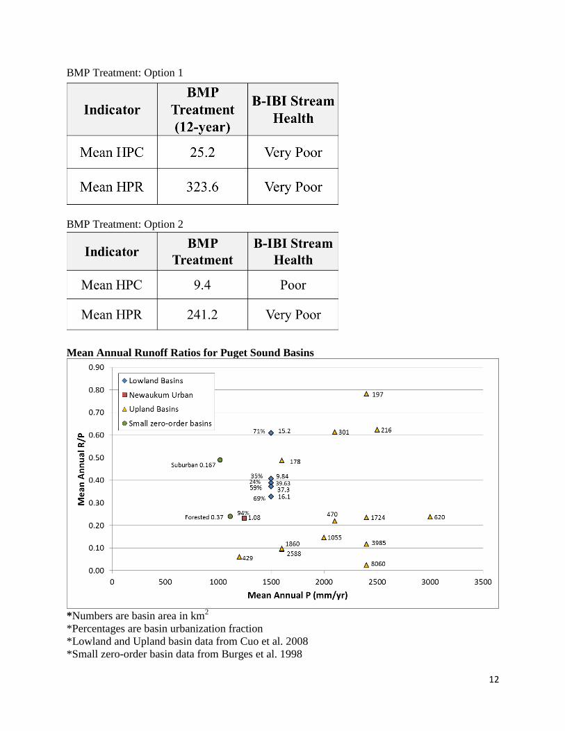
BMP Treatment: Option 1

BMP Treatment: Option 2

Mean Annual Runoff Ratios for Puget Sound Basins

*Numbers are basin area in km

2

*Percentages are basin urbanization fraction

*Lowland and Upland basin data from Cuo et al. 2008

*Small zero-order basin data from Burges et al. 1998

197

39.63 24%

13

References

ASCE-EWRI (2005). The ASCE Standardized Reference Evapotranspiration Equation. Report

of the Task Committee on Standardization of Reference Evapotranspiration. Environmental and

Water Resources Institute of the American Society of Civil Engineers, Reston, Virginia, USA.

DeGasperi et al. (2009). Linking hydrologic alteration to biological impairment in urbanization

streams of the Puget Lowland, Washington, USA. Journal of American Water Resource

Association, 45(2), 512-533.

Boyd, M.J., M. C. Bufill, R. M. Knee (1993). Pervious and impervious runoff in urban

catchments, Hydrological Sciences, 38(6), 463-478.

Boyd, M.J., M. C. Bufill, R. M. Knee (1994). Predicting pervious and impervious storm runoff

from urban drainage basins, Hydrological Sciences, 39(4), 321-332.

Burges, S.J., M.S. Wigmosta, and J.M. Meena (1998). Hydrological effects of land-use change in

a zero-order catchment, Journal of Hydrologic Engineering, 3, 86-97.

Campbell, G. S. (1974). A simple method for determining unsaturated conductivity from

moisture retention data, Soil Sciences, 117, 3311-314.

Chapman, T. (1991). Comment on ‘‘Evaluation of automated techniques for base flow and

recession analyses’’ by R. J. Nathan and T. A. McMahon, Water Resources Research, 27, 1783–

1784.

Cuo, L., D. P. Lettenmaier, B.V. Mattheussen, P. Storck, and M Wiley (2008). Hydrologic

prediction for urban watersheds with the Distributed Hydrology-Soil-Vegetation Model,

Hydrologic Processes, doi: 10.1002/hyp.7023.

Fore, L.S., J.R. Karr. And R.W. Wisseman (1996). Assessing Invertebrate Responses to Human

Activities: Evaluating Alternative Approaches. Journal of the North American Benthological

Society 15(2), 212-231.

Hino, M., and M. Hasabe (1984). Identification and prediction of nonlinear hydrologic systems

by the filter-separation autoregressive (AR) method: extension to hourly hydrologic data,

Journal of Hydrology, 68, 181-210.

Horner, R.R., D.B. Booth, A. Azous, and C.W. May (1997). Watershed Determinants of

Ecosystem Functioning. In L.A. Roesner (ed.), Effects of Watershed Development and

Management on Aquatic Ecosystems, American Society of Civil Engineers, New York, NY, 251-

274.

Horner, R. (2011). Development of Flow and Water Quality Indicators. Unpublished Status

Report.

14

Horner, R. (2012). Development of Flow and Water Quality Indicators. Unpublished Status

Report.

Istanbulluoglu, E., T. Wang, and D. A. Wedin (2012). Evaluation of ecohydrologic model

parsimony at local and regional scales in a semiarid grassland ecosystem, Ecohydrology, 5, 121-

142.

Karr, J.R., and C.O. Yoder (2004). The Biological Assessment and Criteria Improve Total

Maximum Daily Load Decision Making, Journal of Environmental Engineering, 130 (6), 594-

604.

Laio, F., A. Porporato, L. Ridolfi, I Rodriguez-Iturbe (2001). Plants in water controlled

ecosystems: Active role in hydrologic processes and response to water stress II. Probabilistic soil

moisture dynamics, Advances in Water Resources, 24, 707-723.

Linsley, R. K., M.A. Kohler, and J.L.H. Paulhus (1958). Hydrology for Engineers, McGraw-Hill,

New York.

May, C.W. (1996). Assessment of Cumulative Effects of Urbanization on Small Streams in the

Puget Sound Lowland Ecoregion: Implications for Salmonid Resource Management. Ph.D.

dissertation, University of Washington, Seattle, WA, U.S.A.

May, C.W., E.B. Welch, R.R. Horner, J.R. Karr, and B.W. Mar (1997). Quality Indices for

Urbanization Effects in Puget Sound Lowland Streams. Washington Department of Ecology,

Olympia, WA.

Nathan, R. J., and T. A. McMahon (1990). Evaluation of automated techniques for base flow and

recession analyses, Water Resources Research, 26, 1465– 1473.

Smakhtin, V. U. (2001). Low flow hydrology: A review, Journal of Hydrology., 240, 147– 186.

Shoemaker, L., J. Riverson Jr., K. Alvi, J. X. Zhen, S. Paul, and T. Rafi (2009). SUSTAIN - A

Framework for Placement of Best Management Practices in Urban Watersheds to Protect Water

Quality. EPA/600/R-09/095. U.S. Environmental Protection Agency, Water Supply and Water

Resources Division, National Risk Management Research Laboratory, Cincinnati, OH.

Sujono, J., S. Shikasho, and K. Hiramatsu (2004). A comparison of techniques for hydrograph

recession analysis, Hydrological Processes, 18, 403-313.

Wang, T., E. Istanbulluoglu, J. Lenters, and D. Scott (2009). On the role of groundwater and soil

texture in the regional water balance: An investigation of the Nebraska Sand Hills, USA, Water

Resources Research, 45, W10413, doi:10.1029/2009WR007733.