EFFECTS OF CURVATURE ON THE STRESSES by THIEN NGUYEN ...

EFFECTS OF CURVATURE ON THE STRESSES

OF A CURVED LAMINATED BEAMS

SUBJECTED TO BENDING

by

THIEN NGUYEN

Presented to the Faculty of the Graduate School of

The University of Texas at Arlington in Partial Fulfillment

of the Requirements

for the Degree of

MASTER OF SCIENCE IN MECHANICAL ENGINEERING

THE UNIVERSITY OF TEXAS AT ARLINGTON

MAY 2010

iii

ACKNOWLEDGEMENTS

I would like to sincerely thank and appreciate to my supervising professor, Dr. Wen S.

Chan for his guidance, support, and encouragement throughout my research in every aspect.

My gratitude goes to the committee members: Dr. Seiichi Nomura and Dr. Haiying Huang, for

providing guidance and support.

Most of all, thanks to my up coming son, Dat Nguyen, and my beloved wife, Tram

Nguyen, for her love, support, and encouragement. Without her love and support, none of this

research work would have proceeded.

Finally, thanks to my parents, my brothers, and my sisters for their love and support.

April 16, 2010

iv

ABSTRACT

EFFECTS OF CURVATURE ON THE STRESSES

OF A CURVED LAMINATED BEAM

SUBJECTED TO BENDING

Thien Nguyen, M.S.

The University of Texas at Arlington, 2010

Supervising Professor: Wen S. Chan

In aircraft structural applications, curved laminated beam structures are often used as

part of the internal structure. If the curved composite structure is subjected to bending that

tends to flatten or compress the composite structure, interlaminar stresses can be generated in

the thickness direction of the composites. These interlaminar stresses are the major factor of

delamination failure. Besides these stresses, the in-plane stresses can be also affected by the

pre-existence of the beam curvature.

This research has studied the variation of both tangential and radial stresses with

respect to the changing in curvature, stacking sequence, and fiber orientation in a curved

laminated beam subjected to a bending moment. Three 3-D finite element models of the curved

laminated beam have been developed in PATRAN / NASTRAN. These models have been

validated for isotropic material, Al-2014-T6, and orthotropic material, T300/977-2

v

graphite/epoxy, with all 00 plies lay-up. The finite element models of the curved laminated beam

provide solutions showing an excellent agreement with the exact solutions for both tangential

and radial stresses.

An analytical method to calculate the tangential stress was also developed for a curved

laminated beam subjected to a bending moment. The tangential stress results from this method

were compared well with the results from the finite element method. The analytical closed-form

expressions of axial, coupling and bending stiffness, as well as their characteristics were also

investigated.

vi

TABLE OF CONTENTS

ACKNOWLEDGEMENTS ................................................................................................................iii ABSTRACT ..................................................................................................................................... iv LIST OF ILLUSTRATIONS.............................................................................................................. ix LIST OF TABLES............................................................................................................................xii Chapter Page

1. INTRODUCTION……………………………………..………..…........................................1

1.1 Composite Material Overview ..........................................................................1

1.1.1 History ..............................................................................................1

1.1.2 Definition and Applications...............................................................1

1.1.3 Curved Laminated Beam .................................................................2 1.1.4 Past works in Composite Curved Beam ..........................................3

1.2 Objectives and Approach to the Thesis ...........................................................6

1.3 Outline of the Thesis ........................................................................................8

2. FINITE ELEMENT MODEL ............................................................................................9

2.1 Geometry and Material Used ...........................................................................9

2.1.1 Geometry of Curved Laminated Beam ............................................9 2.1.2 Material of Composite Laminate ....................................................10

2.2 Development of Finite Element Model ...........................................................12

2.2.1 Modeling Creation ..........................................................................12 2.2.2 Meshing Generation.......................................................................13 2.2.3 Creation of Local Coordinate Systems ..........................................15 2.2.4 Boundary and Loading Conditions.................................................16

2.3 Model Validation.............................................................................................17

vii

2.3.1 Isotropic Material............................................................................17 2.3.1.1 FEM Result ....................................................................17 2.3.1.2 Exact Solution ................................................................19

2.3.2 Orthotropic Material........................................................................23

2.4 Convergence..................................................................................................26

3. ANALYTICAL METHOD FOR CURVED LAMINATED BEAM.....................................28

3.1 Review of Lamination Theory.........................................................................28

3.1.1 Elastic Stress-Strain Relationship of Lamina.................................29 3.1.2 Constitutive Equation of Laminate (Lamination Theory)................31

3.2 Curved Laminated Beam ...............................................................................33

4. STRESS EFFECT OF CURVATURE AND STACKING SEQUENCE.........................35

4.1 The Curvature Effect on Laminate Stresses ..................................................35

4.1.1 Stress Distribution ..........................................................................35

4.1.1.1 Stress Distribution for 00 ply...........................................37 4.1.1.2 Stress Distribution for -450 ply and +450 ply ..................38 4.1.1.3 Stress Distribution for 900 ply.........................................40

4.1.2 Stress Comparison.........................................................................41

4.1.2.1 The Stress Variation for +450 ply#1 ...............................42 4.1.2.2 The Stress Variation for -450 ply#2 ................................44 4.1.2.3 The Stress Variation for 900 ply#4 .................................46 4.1.2.4 The Stress Variation for 00 ply#6 ...................................48

4.1.3 Stacking Sequence [+450/-450/900

2/002]S .......................................50

4.2 The Fiber Orientation Effect on Laminate Stresses.......................................51

4.2.1 Symmetric and Balanced Laminates .............................................51 4.2.2 Symmetric / Unsymmetrical and Balanced / Unbalanced

Laminates .......................................................................................54

viii

4.3 The Effect of Stacking Sequence...................................................................56

5. CONCLUSIONS AND FUTURE WORK ......................................................................58

APPENDIX

A. GENERAL PROCEDURE TO CREATE A 3D FEM FOR AN ISOTROPIC AND A CURVED LAMINATED BEAM IN PATRAN ..............................................................61

B. MATHEMATICAL PROCEDURE TO VERIFY THE ACCURACY OF MATRIX [A], [B], AND [D] WHEN THE CURVATURE GOES TO INFINITY...............................70

REFERENCES...............................................................................................................................76 BIOGRAPHICAL INFORMATION ..................................................................................................77

ix

LIST OF ILLUSTRATIONS

Figure Page 1.1 Examples of aircraft structural components...............................................................................3 1.2 Opening and Closing modes of composite curved beam. .........................................................6 1.3 Interlaminar stresses in radius region ........................................................................................7 2.1 Iso view of 3-D curved beam......................................................................................................9 2.2 Pure bending loading ...............................................................................................................10 2.3 The creation of 12 surfaces......................................................................................................13 2.4 The defined mesh seeds of 3-D solid model............................................................................13 2.5 Hex 8 element ..........................................................................................................................14 2.6 Isomesh of 3-D solid model......................................................................................................14 2.7 30 Groups of elements along the transverse direction ............................................................15 2.8 The creation of local coordinate for each ply ...........................................................................16 2.9 Two boundary conditions respect to global coordinate system ...............................................17 2.10 Center group and its radial and circumferential directions.....................................................18 2.11 Curved beam subjected to bending moment and its cross section .......................................20 2.12 Radial stress comparison between isotropic FEM and exact solution...................................22 2.13 Tangential stress comparison between isotropic FEM and exact solution ............................22 2.14 Local coordinate system for each element group ..................................................................23 2.15 Radial stress comparison for isotropic, orthotropic and exact solution..................................25 2.16 Tangential stress comparison for isotropic, orthotropic and exact solution ...........................25 2.17 Selected center group ............................................................................................................26 2.18 The convergence of tangential stress ....................................................................................27 2.19 The convergence of radial stress ...........................................................................................27

x

3.1 Coordinate systems of lamina and laminate ............................................................................29 3.2 Element of single layer with force and moment resultants.......................................................31 3.3 Laminate plate geometry and layer numbering system ...........................................................32 3.4 The configurations of curved beam and its cross section........................................................33 4.1 The lay-up sequence of composite curved beam ....................................................................36 4.2 The distribution of tangential stress σθ in 00 ply .......................................................................37 4.3 The distribution of radial stress σr in 00 ply ..............................................................................37 4.4 The distribution of tangential stress σθ in -450 ply....................................................................38 4.5 The distribution of radial stress σr in -450 ply ...........................................................................38 4.6 The distribution of tangential stress σθ in +450 ply ...................................................................39 4.7 The distribution of radial stress σr in +450 ply ..........................................................................39 4.8 The distribution of tangential stress σθ in 900 ply .....................................................................40 4.9 The distribution of radial stress σr in 900 ply ............................................................................40 4.10 Elements on each ply at different angle position ...................................................................41 4.11 Tangential stress for +450 lay-up ...........................................................................................43 4.12 Radial stress for +450 lay-up ..................................................................................................43 4.13 Tangential stress for -450 lay-up ............................................................................................45 4.14 Radial stress for -450 lay-up...................................................................................................45 4.15 Tangential stress for 900 lay-up..............................................................................................47 4.16 Radial stress for 900 lay-up ....................................................................................................47 4.17 Tangential stress for 00 lay-up................................................................................................49 4.18 Radial stress for 00 lay-up ......................................................................................................49 4.19 Description of laminate coding for five different stacking sequences ....................................51 4.20 The selected elements in 900 layer #6 at different angle positions........................................52 4.21 Stress for element at 270 angle position ................................................................................52 4.22 Stress for element at 330 angle position ................................................................................53

xi

4.23 Stress for element at 390 angle position ................................................................................53 4.24 Description of laminate coding for three different stacking sequences..................................54 4.25 The variation of tangential stress ...........................................................................................55

xii

LIST OF TABLES

Table Page 2.1 Geometric parameters for three different curved beam models ..............................................10

2.2 Required material properties for NASTRAN MAT 9 Card........................................................10

2.3 Material properties for Graphite/Epoxy at 700 F Ambient ........................................................11 2.4 Material properties for Graphite/Epoxy at 700 F Ambient in NASTRAN MAT 9.......................12 2.5 Material properties for Al-2014-T6 in NASTRAN MAT 1..........................................................18 2.6 The recorded stress values from FEM for isotropic material ...................................................19 2.7 Dimensions of curved beam model..........................................................................................19 2.8 The calculated stress values from exact solution ....................................................................21 2.9 The recorded stress values from FEM for orthotropic material................................................24 4.1 Ply sequence for 12-ply composite curved beam ....................................................................36 4.2 The stress values for +450 ply#1..............................................................................................42 4.3 The stress values for -450 ply#2...............................................................................................44 4.4 The stress values for 900 ply#4................................................................................................46 4.5 The stress values for 00 ply#6..................................................................................................48 4.6 The comparison for tangential stress .......................................................................................50 4.7 Laminate stacking sequences..................................................................................................56 4.8 Matrices comparison for laminate 3 .........................................................................................56 4.9 Matrices comparison for mid-plane radius R1 = 0.2444 inches ...............................................57 4.10 Matrices comparison for laminate 3 & 5.................................................................................57

1

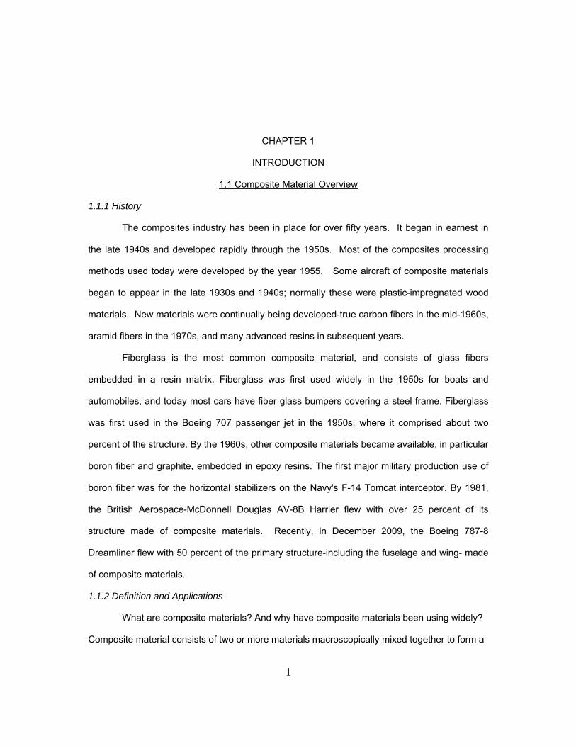
CHAPTER 1

INTRODUCTION

1.1 Composite Material Overview

1.1.1 History

The composites industry has been in place for over fifty years. It began in earnest in

the late 1940s and developed rapidly through the 1950s. Most of the composites processing

methods used today were developed by the year 1955. Some aircraft of composite materials

began to appear in the late 1930s and 1940s; normally these were plastic-impregnated wood

materials. New materials were continually being developed-true carbon fibers in the mid-1960s,

aramid fibers in the 1970s, and many advanced resins in subsequent years.

Fiberglass is the most common composite material, and consists of glass fibers

embedded in a resin matrix. Fiberglass was first used widely in the 1950s for boats and

automobiles, and today most cars have fiber glass bumpers covering a steel frame. Fiberglass

was first used in the Boeing 707 passenger jet in the 1950s, where it comprised about two

percent of the structure. By the 1960s, other composite materials became available, in particular

boron fiber and graphite, embedded in epoxy resins. The first major military production use of

boron fiber was for the horizontal stabilizers on the Navy's F-14 Tomcat interceptor. By 1981,

the British Aerospace-McDonnell Douglas AV-8B Harrier flew with over 25 percent of its

structure made of composite materials. Recently, in December 2009, the Boeing 787-8

Dreamliner flew with 50 percent of the primary structure-including the fuselage and wing- made

of composite materials.

1.1.2 Definition and Applications

What are composite materials? And why have composite materials been using widely?

Composite material consists of two or more materials macroscopically mixed together to form a

2

useful new material. This new material contains on constituent to reinforce the other

constituent. The composite reinforcement is often in the form of continuous fibers which are

high specific stiffness and strength. To take advantages of these unique properties of the fiber

reinforced composites, a structure often contains multiple layers laminated together with each

layer oriented in the direction of the pre-determined structural function. Due to lack of the

thickness reinforcement, laminate is prone to delamination resulting in loss of stiffness, strength

and fatigue life.

Composite materials are now the most preferred materials in aircraft structures. Many

aircraft are currently undergoing the design that takes advantage of composite materials for

primary structure applications. Composites are different from metals in several ways. These

include their largely elastic response, their ability for tailoring of strength and stiffness, their

damage tolerance characteristics, and their sensitivity to environmental factors. However,

unlike metals, composite materials often give little or no warning before weakening the

structural members in aircraft.

1.1.3 Curved Laminated Beam

Most of structural components in aircraft structures in general and in composite

structures in particular could contain curved beam regions or could be in the form of curved

panels. In structural applications, beam is one of the primary structures that used to support the

bending and transverse loads. Beams can be straight or curved. Examples include Z-stiffener,

angle clip, angle bracket and panel with supporting stringers in aircraft system, as shown in

Figure 1.1. Improper design of these curved beam/panel structures may lead to structural

failures.

3

Figure 1.1. Examples of aircraft structural components.

1.1.4 Past works in Composite Curved Beam

Numerous of studies, researches had been done in the linear/or nonlinear for straight beams.

However, much less works have been done for the laminated beams, particularly the curved

beams.

Sayegh and Dong [1] in 1970 investigated the stresses and displacements of a three-

layer curved beam subjected to loading conditions of pure flexure and applied axial force using

both technical theory and orthotropic elasticity. It was shown that for a beam, whose radius of

curvature is large compared to the total thickness, technical theory gives adequate results

provided the properties of the layer are approximately the same. For large differences, the

prediction by the technical theory may be in considerable error.

Cheung and Sorensen [2] provided additional insight into the effect on the radial

stresses due to the axial loads that are present in the curved beams. Equations of tangential,

Angle Clip

Angle Bracket

Radius region

Z-Stiffener

Panel with supporting stringers

Angle Clip

Angle Bracket

Radius region

Z-Stiffener

Panel with supporting stringers

4

radial, and shear stress were developed for curved beams under an axial load. The theory of

elasticity with polar coordinates for plane stress applied to an orthotropic material was used.

The theoretical radial stresses predicted by Wilson's equation were verified by a rigorous theory

of elasticity solution as both solutions gave almost identical results. They concluded that the

effect of axial load on the radial stress in curved beams is small.

Graff and Springer [3] developed a finite element code to calculate the stresses and

strains in thick, curved composite laminates subjected to an arbitrary, but consistent,

combination of forces and displacements. The analysis was formulated using anisotropic,

bilinear quadrilateral and tri-linear hexahedral continuum elements. A computer code was then

written for either three-dimensional or two-dimensional (plane stress or plane strain) analysis of

curved laminates. The accuracy of the computer code was evaluated by generating numerical

results for three problems for which analytical solutions exist, and by comparing the numerical

and analytical results. In every case the agreement between the numerical and analytical

results was excellent.

Barbero et al. [4] investigated the bending behavior of glass fiber reinforced composite

beam. They showed that the bending stiffness is low compared to that of steel sections of the

same shape. They concluded that shear deformation effects are important for composite

beams. This is due to relatively low elastic modulus of glass fibers when compared to steel and

the low shear modulus of matrix resin.

Madabhusi-Raman and Davalos [5] later derived a form for the shear correction factor

for laminated rectangular beams with symmetric or asymmetric cross-ply or angle-ply lay-ups. In

this work, the shear correction factor was computed by equating the shear strain energy

obtained from the constitutive relations of first order shear deformable laminated plate theory to

that obtained using the “actual” shear stress distribution calculated a posteriori, i.e. computed

using the equilibrium equations of elasticity.

5

Kasal and Heiduschle [6] studied the application of fiber composite materials in

reinforcement of laminated wood arches subjected to radial tension. An experimental program

was designed that included testing of mechanical properties of composite tubes, studying

properties of the wood-composite tube interface, testing of the wood-steel rod interface, and

testing of models of laminated wood arches. The application of composite materials in radial

reinforcement of arches is feasible and possibly has advantages over the glued-in steel rods

because of greater flexibility of sizes and properties of reinforcing elements, low mass, and

potential ease of installation.

Wang and Shenoi [7] studied the through-thickness tension in curved sandwich beam

using an elasticity-theory-based approach. This approach ensures an accurate description of

the through-thickness stresses in curved sandwich beam. The critical load for instability of a

curved beam on an elastic foundation which is correspondent to the skin of sandwich beam, is

considered and compared with the result for a flat beam on an elastic foundation. Wang and

Shenoi also studied the flexural strength of sandwich beam to identify debonding and local

instability characteristics. The effects of various parameters, such as geometrical configuration,

stiffness of the skin and core, on through-thickness tension stress and local instability

respectively are included in this study.

Qatu [8] in 2004 addressed the vibration of laminated curved beams and rings

subjected to combined loading, bending and shear loads. The fundamental equations and

energy functional for laminated curved beams and closed rings were developed and presented

in both exact and approximate solutions. These equations are very useful for design engineers.

6

1.2 Objectives and Approach to the Thesis

The composite curved beam regions are vulnerable to out-of-plane failures. Loads

which tend to open or close the curved beam regions result in tensile or compressive radial

stress, respectively, as shown in Figure 1.2.

Figure 1.2. Opening and Closing modes of composite curved beam.

The typical failure mode for this region is delamination in the radius area. Delamination

is one of the major causes of failure in laminated composite structures, in which the layers of

the material separate from each other. Delamination can be caused by interlaminar shear

stresses ( θτ r ) between the layers, or tensile radial stresses ( rσ ) across the layers. Tensile

radial stress (out-of-plane stress) is the principal cause of delamination in the composite curved

beam structures (see Figure 1.3). Once the delamination takes place, the composite structure

could lose their strength and stiffness significantly, and may lead to a catastrophic structural

collapse.

7

Figure 1.3. Interlaminar stresses in radius region.

Interlaminar stress is a key parameter to be taken into consideration for any composite

structural design, especially for structures that contain radius areas. Composite structures are

often optimized for minimum weight and maximum strength. Thus, design of composite

structures to meet the structural specifications is a challenge problem. Understanding the

behavior of the interlaminar stresses in the composite curved beam structures is significant to

structural design in many fields. The variation of interlaminar stresses can lead to the changing

in geometry design of structural components. Thus, interlaminar stresses must be considered

in the design, validation, and certification phases of airframe development.

The primary objective of this study is to investigate the laminate stresses in a curved

laminated beam subjected to a pure bending moment. The study was focused on both radial

stress (out-of-plane stress) and tangential stress (in-plane stress) effects due to the curvatures,

stacking sequences and fiber orientations. An approximated closed-form relationship of

laminate constitutive equation is developed to understanding the characteristics of a curved

laminate. A 3-D finite element model of PATRAN / NASTRAN was developed to investigate

both radial and tangential stress distribution.

This study intended to provide the better understanding about the variation of radial

and tangential stresses due to laminate curvature, stacking sequence, and fiber orientation in

the curved beam.

8

1.3 Outline of the Thesis

Chapter 2 presents procedure to develop the geometry, the 3-D finite element model,

the material used and its boundary conditions. The validation of analyzed model and the

convergence for stresses are also included.

Chapter 3 presents a brief review of lamination theory. An analytical method to

calculate the tangential ply stress in a curved laminated beam is presented.

Effects of the tangential and radial ply stresses with the variation of curvature are

included in Chapter 4. Effects of the ply stresses due to stacking sequence such as

symmetrical versus unsymmetrical and balanced versus unbalanced are also investigated in

this Chapter. A comparison of the results between the analytical method and FEM method is

included in this Chapter as well.

Chapter 5 concludes the work and provides a future work.

9

CHAPTER 2

FINITE ELEMENT MODEL

This Chapter describes in detail the geometry, material used in the model, how the

model constructed, and the boundary conditions used. PATRAN / NASTRAN was used to

develop the required 3-D finite element model.

2.1 Geometry and Material Used

2.1.1. Geometry of Curved Laminated Beam

Three semicircular curved beam models with different curvatures were constructed.

The dimensions of these three models are listed in Table 2.1. Figure 2.1 shows the geometry of

a typical curved beam 3-D model.

Figure 2.1. Iso view of 3-D curved beam.

10

Table 2.1. Geometric parameters for three different curved beam models.

Configuration Inner Radius, Ri (inches)

Outer Radius, Ro (inches)

Mid-Plane Curvature, R

(inches)

Width w (inches)

Model I 0.2 0.2888 0.2444 1 Model II 0.6 0.6888 0.6444 1 Model III 1.8 1.8888 1.8444 1

Figure 2.2. Pure bending loading.

2.1.2 Material of Composite Laminate

The material properties required to define the NASTRAN MAT9 card are shown in

Table 2.2 below. Four MAT9 cards are used for the curved beam, one for 00-ply elements, one

for 900-ply elements, one for the -450-ply elements, and one for the +450-ply elements.

Table 2.2. Required material properties for NASTRAN MAT 9 Card

Required Material Properties E1 E2 E3 v12 v23 v31 G12 G23 G31

Material 1, Material 2, and Material 3 Directions Correspond to the Element Material Directions Defined in Figure 2.1 & 2.7.

11

The material used for a laminate composite is T300/977-2 graphite/epoxy. The lay-up of the

laminate is chosen as symmetric and balanced laminate to eliminate the coupling effects of

bending and shear in the flat laminate. The stacking sequence is [-45/+45/902/02]S. The

unidirectional orthotropic material properties for graphite/epoxy at 700F/ambient temperature are

tabulated in Table 2.3.

Table 2.3. Material properties for Graphite/Epoxy at 700 F Ambient

The constants E1, E2 and E3 are the nominal Young moduli of composite ply. The subscripts 1,

2, and 3 are fiber direction, transverse to the fiber direction, and out-of-plane direction,

respectively. The constants G12, G23 and G13 are the shear moduli with respect to 1-2, 2-3, and

1-3 planes, respectively. The constants 12ν , 13ν and 23ν are Poisson’s ratios. Material property

values for the NASTRAN MAT9 card per Table 2.2 requirement are derived from the

graphite/epoxy lamina property values tabulated in Table 2.4.

Lamina Properties for Graphite/Epoxy at 700F/Ambient E1 = 21.75 Msi E2 = 1.595 Msi E3 = 1.595 Msi

12ν = 0.25

13ν = 0.25

23ν = 0.45 G12 = 0.8702 Msi G23 = 0.5366 Msi G13 = 0.8702 Msi tply = 0.0074 in


12

Table 2.4. Material properties for Graphite/Epoxy at 700 F Ambient in NASTRAN MAT 9

Material Properties for NASTRAN MAT9 for Graphite/Epoxy at 700F/Ambient

E1 = 21.75 Msi

E2 = 1.595 Msi

E3 = 1.595 Msi

12ν = 0.25

31ν = 0.0183

23ν = 0.45 G12 = 0.8702 Msi

G23 = 0.5366 Msi

G31 = 0.8702 Msi

tply = 0.0074 in


Where, 0183.075.21

595.125.01

31331 =×=×=

EE

υυ

2.2 Development of Finite Element Model

2.2.1 Modeling Creation

PATRAN has been used to develop the 3-D solid finite element model. PATRAN uses

the Global Model Tolerance when it creates geometry. The default value is 0.005. When

creating geometry, if two points are within a distance of the Global Model Tolerance, then

PATRAN will only create the first point and not the second. This rule also applies to curves,

surfaces, and solids. Due to the thickness of each ply in the curved beam model is 0.0074 inch

(greater than the default value 0.005), the Global Model Tolerance is set at 0.0005 to improve

the model usability. The procedure for generating 3-D Solid FEM for this study is shown below.

1. The 1ST curved surface with inner radius Ri was created.

2. Then 11 more curved surfaces were created by using the “Normal to Surface” method. The

distance between each surface is 0.0074 inches.

3. 12 solids were created from these 12 surfaces with the thickness of 0.0074 for each solid.

13

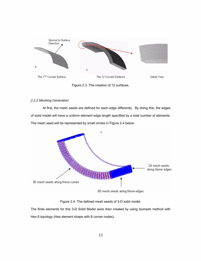
Figure 2.3. The creation of 12 surfaces.

2.2.2 Meshing Generation

At first, the mesh seeds are defined for each edge differently. By doing this, the edges

of solid model will have a uniform element edge length specified by a total number of elements.

The mesh seed will be represented by small circles in Figure 2.4 below.

Figure 2.4. The defined mesh seeds of 3-D solid model.

The finite elements for this 3-D Solid Model were then created by using Isomesh method with

Hex 8 topology (Hex element shape with 8 corner nodes).

14

Figure 2.5. Hex 8 element.

This Isomesh created equally-spaced nodes along each edge in the model. A real value will be

assigned to the element edge length for a given mesh. This value is known as global element

edge length. This global element edge length was calculated automatically as 0.0264. This

value can be adjusted in case of encounter difficulties.

The action of equivalence was applied for the entire model with equivalencing tolerance of

0.0005 to delete any duplicated nodes or extra nodes in the model. This 3-D Solid Model

contains 43200 Hex 8 elements with the aspect ratio of 9.7 for all elements generated. The

meshing is shown in Figure 2.6 below.

Figure 2.6. Isomesh of 3-D solid model.

15

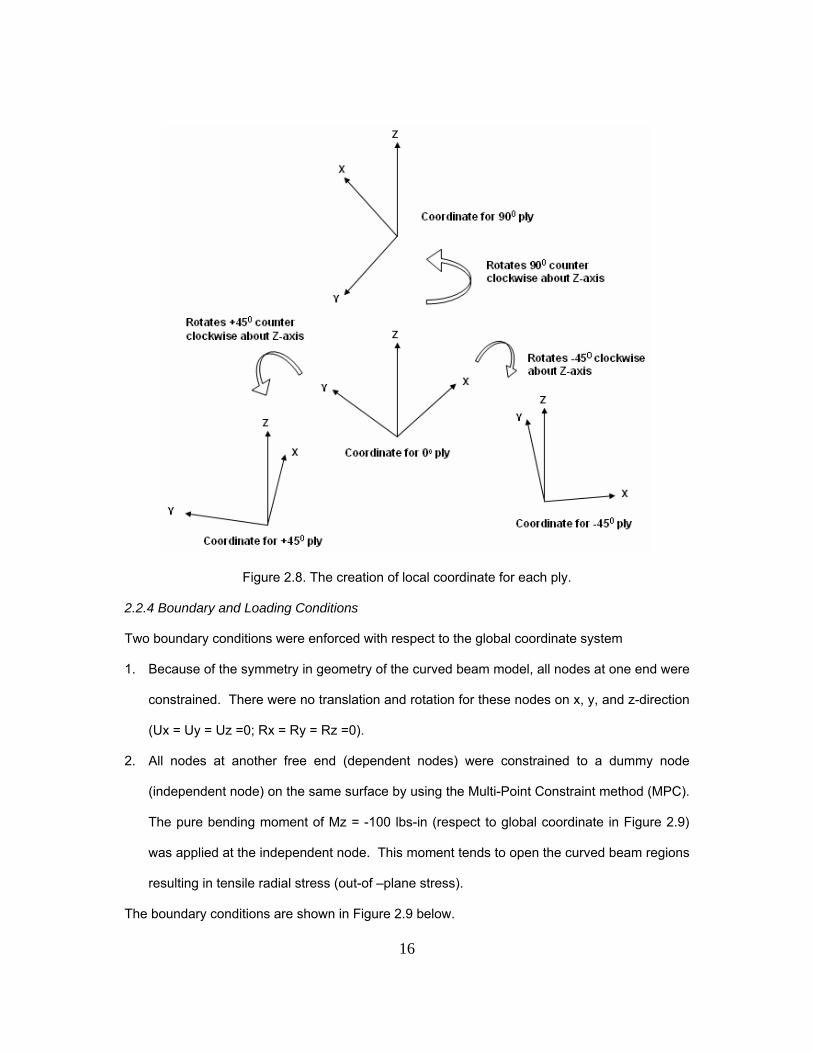
2.2.3 Creation of Local Coordinate Systems

The composite curve beam is modeled by NASTRAN 3-D CHEXA Solid elements. The

curved beam model contains 12 plies lay-up. Each ply is explicitly modeled by two rows of

elements. The model was divided into 30 groups, as shown in Figure 2.7. By doing this, the

curved beam is represented by several straight beam elements. Each group was assigned to

different local coordinate systems, corresponding to the angle of fiber orientation of each layer

of laminated composite. The material X-direction, Y-direction and Z-direction for the elements

in the curved beam model were established to be the fiber direction (material direction 1), the

transverse to the fiber direction (material direction 2) and the out-of plane direction (material

direction 3), respectively. Four local coordinate systems were assigned to each element group.

At first, a local coordinate was created for 00 ply. Then, this local coordinate was rotated at -450,

+450 and 900. This procedure created four different local coordinates which associate to four

different angle of fiber orientation: 00, -450, +450 and 900. The creation of local coordinates for

each element group is shown in Figure 2.8.

Figure 2.7. 30 Groups of elements along the transverse direction.

16

Figure 2.8. The creation of local coordinate for each ply.

2.2.4 Boundary and Loading Conditions

Two boundary conditions were enforced with respect to the global coordinate system

1. Because of the symmetry in geometry of the curved beam model, all nodes at one end were

constrained. There were no translation and rotation for these nodes on x, y, and z-direction

(Ux = Uy = Uz =0; Rx = Ry = Rz =0).

2. All nodes at another free end (dependent nodes) were constrained to a dummy node

(independent node) on the same surface by using the Multi-Point Constraint method (MPC).

The pure bending moment of Mz = -100 lbs-in (respect to global coordinate in Figure 2.9)

was applied at the independent node. This moment tends to open the curved beam regions

resulting in tensile radial stress (out-of –plane stress).

The boundary conditions are shown in Figure 2.9 below.

17

Figure 2.9. Two boundary conditions respect to global coordinate system.

2.3 Model Validation

The purpose of this section is to validate the curve beam FEM using the closed-form

solution. The geometry, meshing, elements, boundary conditions, and loading conditions for

this curve beam remained the same as defined in the sections above.

2.3.1 Isotropic Material

2.3.1.1 FEM Result

An isotropic material, Al-2014-T6, was used instead of T300/977-2 graphite/epoxy.

Because of the uniformity in all directions, one cylindrical coordinate system was used for the

entire model. The material properties for Al-2014-T6 are shown in Table 2.5.

18

Table 2.5. Material properties for Al-2014-T6 in NASTRAN MAT 1

Material Properties for NASTRAN MAT1

for Al-2014-T6E 10.6 Msi ν 0.35 G 3.9 Msi

For the most accuracy in the results from FEM, a group of through thickness elements in the

middle of the model was selected to eliminate the “edge effective”.

Figure 2.10. Center group and its radial and circumferential directions.

The radial stress and tangential (along circumferential direction) stress at the Centroid of each

element in center group, as shown in Figure 2.10, were recorded from the output results in

PATRAN. Table 2.6 summarizes these stresses respect to radial position (the distance from

the center of curved beam, as shown in Figure 2.14, to the centroid of each element).

19

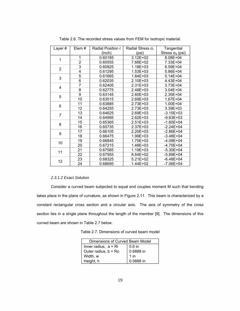
Table 2.6. The recorded stress values from FEM for isotropic material.

Layer # Elem # Radial Position r (inch)

Radial Stress σr (psi)

Tangential Stress σθ (psi)

1 0.60185 3.12E+02 8.08E+04 1 2 0.60555 7.68E+02 7.33E+04 3 0.60925 1.18E+03 6.59E+04 2 4 0.61295 1.53E+03 5.86E+04 5 0.61665 1.84E+03 5.14E+04 3 6 0.62035 2.10E+03 4.43E+04 7 0.62405 2.31E+03 3.73E+04 4 8 0.62775 2.48E+03 3.04E+04 9 0.63145 2.60E+03 2.35E+04 5 10 0.63515 2.69E+03 1.67E+04 11 0.63885 2.73E+03 1.00E+04 6 12 0.64255 2.73E+03 3.39E+03 13 0.64625 2.69E+03 -3.15E+03 7 14 0.64995 2.62E+03 -9.63E+03 15 0.65365 2.51E+03 -1.60E+04 8 16 0.65735 2.37E+03 -2.24E+04 17 0.66105 2.20E+03 -2.86E+04 9 18 0.66475 1.99E+03 -3.48E+04 19 0.66845 1.75E+03 -4.09E+04 10 20 0.67215 1.48E+03 -4.70E+04 21 0.67585 1.19E+03 -5.30E+04 11 22 0.67955 8.64E+02 -5.89E+04 23 0.68325 5.21E+02 -6.48E+04 12 24 0.68695 1.44E+02 -7.06E+04

2.3.1.2 Exact Solution

Consider a curved beam subjected to equal end couples moment M such that bending

takes place in the plane of curvature, as shown in Figure 2.11. This beam is characterized by a

constant rectangular cross section and a circular axis. The axis of symmetry of the cross

section lies in a single plane throughout the length of the member [9]. The dimensions of this

curved beam are shown in Table 2.7 below.

Table 2.7. Dimensions of curved beam model

Dimensions of Curved Beam Model Inner radius, a = Ri 0.6 in Outer radius, b = Ro 0.6888 in Width, w 1 in Height, h 0.0888 in

20

Figure 2.11. Curved beam subjected to bending moment and its cross section.

The radial and tangential stresses were calculated by following equations:

⎥⎦

⎤⎢⎣

⎡⎟⎠⎞

⎜⎝⎛⋅⎟⎟

⎠

⎞⎜⎜⎝

⎛−−⎟

⎠⎞

⎜⎝⎛⋅⎟⎟

⎠

⎞⎜⎜⎝

⎛−⋅=

ab

ra

ar

ba

NtbM

r ln1ln142

2

2

2

2σ

⎥⎦

⎤⎢⎣

⎡⎟⎠⎞

⎜⎝⎛⋅⎟⎟

⎠

⎞⎜⎜⎝

⎛+−⎟

⎠⎞

⎜⎝⎛ +⋅⎟⎟

⎠

⎞⎜⎜⎝

⎛−⋅=

ab

ra

ar

ba

NtbM ln1ln114

2

2

2

2

2θσ (Section 5.13, [9])

Where, ⎟⎠⎞

⎜⎝⎛−⎟⎟

⎠

⎞⎜⎜⎝

⎛−=

ab

ba

baN 2

2

22

2

2

ln41 ,

100=M inlbs − , and oi RrR << ; ( iRa = ; oRb = )

These equations are applicable throughout the curved beam. The radial stresses rσ as

determined from the equation above are found positive (tensile). The tangential stresses θσ

are found positive (tensile) for the elements below the mid-plane, and negative (compressive)

for the elements above the mid-plane, as shown in Figure 2.11. Table 2.8 summarizes the

calculated radial stresses rσ and tangential stresses θσ with respect to 24 different radial

positions.

21

Table 2.8. The calculated stress values from exact solution.





The radial stresses and tangential stresses in Table 2.6 and Table 2.8 were plotted in two

different graphs with respect to the variation of radial positions for comparison purposes. The

graphs in Figure 2.12, and Figure 2.13, as shown on the next page, show a good agreement

between FEM results for isotropic material and Exact solutions. Since these results compared

well, the isotropic curved beam model is validated.

22

Figure 2.12. Radial stress comparison between isotropic FEM and exact solution.

Figure 2.13. Tangential stress comparison between isotropic FEM and exact solution.

Exact vs. FEM

0.00E+00

5.00E+02

1.00E+03

1.50E+03

2.00E+03

2.50E+03

3.00E+03

0.59 0.60 0.61 0.62 0.63 0.64 0.65 0.66 0.67 0.68 0.69 0.70

Radial position

Rad

ial S

tres

s

Exact SolutionFEM_Result

Exact vs. FEM

-8.00E+04

-6.00E+04

-4.00E+04

-2.00E+04

0.00E+00

2.00E+04

4.00E+04

6.00E+04

8.00E+04

1.00E+05

0.59 0.60 0.61 0.62 0.63 0.64 0.65 0.66 0.67 0.68 0.69 0.70

Radial position

Tang

entia

l Str

ess

Exact SolutionFEM_Result

23

2.3.2 Orthotropic Material

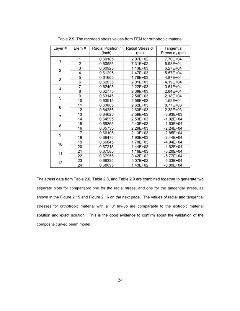
An orthotropic material, T300/977-2 graphite/epoxy, was used. The required material

properties for NASTRAN MAT9 Card are shown in Table 2.4. All 00 plies lay-up was applied for

this curved beam model. The material properties of T300/977-2 graphite/epoxy for 00-ply

elements were assigned to a different element group associated with a different local coordinate

system. There were thirty element groups associated with thirty local coordinate systems.

Figure 2.14. Local coordinate system for each element group.

The material X-direction (perpendicular to the Y-Z plane), Y-direction, and Z-direction were

established to be the fiber direction, the transverse to fiber direction and the out-of plane

direction, respectively. The behavior of the curved beam with the orthotropic material contains

all 00 plies lay-up similar to the curved beam with the isotropic material. The recorded radial

and tangential stress values, as shown in Table 2.9, were compared to the results from the

isotropic material and exact solution in Section 2.3.1.

24

Table 2.9. The recorded stress values from FEM for orthotropic material





The stress data from Table 2.6, Table 2.8, and Table 2.9 are combined together to generate two

separate plots for comparison: one for the radial stress, and one for the tangential stress, as

shown in the Figure 2.15 and Figure 2.16 on the next page. The values of radial and tangential

stresses for orthotropic material with all 00 lay-up are comparable to the isotropic material

solution and exact solution. This is the good evidence to confirm about the validation of the

composite curved beam model.

25

Stress Comparison

0.00E+00

5.00E+02

1.00E+03

1.50E+03

2.00E+03

2.50E+03

3.00E+03

0.59 0.60 0.61 0.62 0.63 0.64 0.65 0.66 0.67 0.68 0.69 0.70

Radial position

Rad

ial S

tres

s

Exact SolutionFEM OrthotropicFEM Isotropic

Figure 2.15. Radial stress comparison for isotropic, orthotropic and exact solution.

Stress Comparison

-8.00E+04

-6.00E+04

-4.00E+04

-2.00E+04

0.00E+00

2.00E+04

4.00E+04

6.00E+04

8.00E+04

1.00E+05

0.59 0.60 0.61 0.62 0.63 0.64 0.65 0.66 0.67 0.68 0.69 0.70

Radial position

Tang

entia

l Str

ess

Exact SolutionFEM OrthotropicFEM Isotropic

Figure 2.16. Tangential stress comparison for isotropic, orthotropic and exact solution.

26

2.4 Convergence

The convergence study was conducted for an isotropic semicircular curved beam,

Model I (mid-plane curvature R1 = 0.2444 inches). The geometry dimensions of this Model I are

shown in Table 2.1. The isotropic material, Al-2014-T6, was used. Due to the uniformity in all

direction of isotropic material, one cylindrical coordinate system was used for the entire model.

The meshing, boundary conditions, and loading conditions remained the same as defined in

Section 2.2. This curved beam model contains 12 plies. Each ply is explicitly modeled by one

row of element. The mesh of this analyzed curved beam model was refined six times. The

number of elements was recorded as: 5400, 7200, 9000, 10800, 12600, and 14400 elements.

The tangential (in-plane) stress and radial (out-of-plane) stress of twelve different elements from

selected center group (through thickness) in this curved beam model were examined. The

values of these stresses were recorded and plotted for convergence examination.

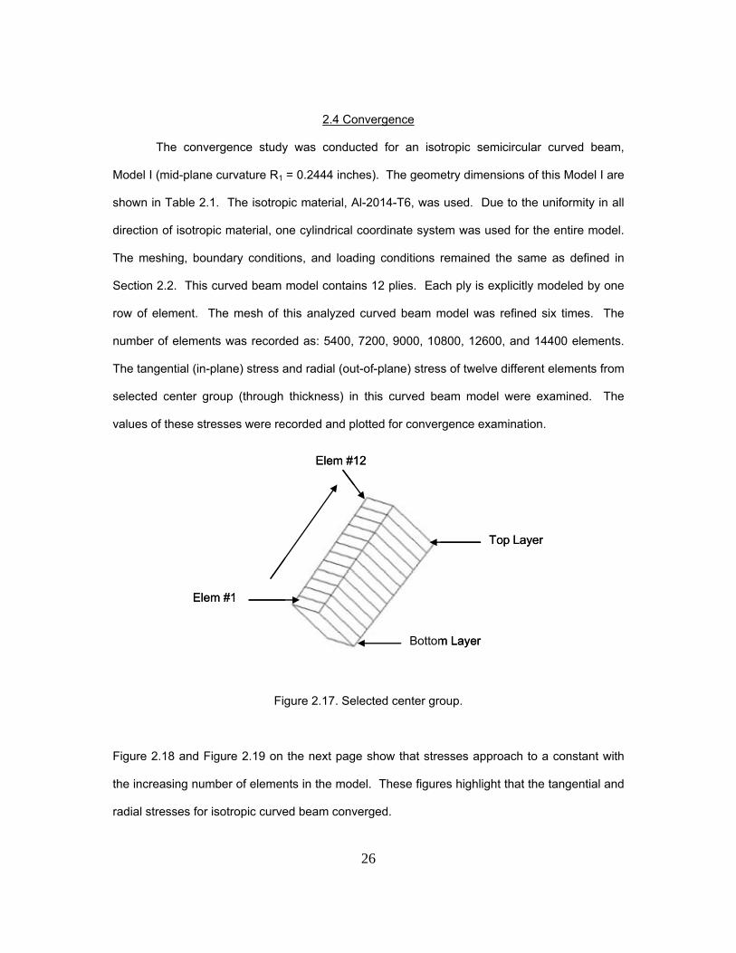
Figure 2.17. Selected center group.

Figure 2.18 and Figure 2.19 on the next page show that stresses approach to a constant with

the increasing number of elements in the model. These figures highlight that the tangential and

radial stresses for isotropic curved beam converged.

Elem #1

Elem #12

Top Layer

Bottom Layer

Elem #1

Elem #12

Top Layer

Bottom Layer

27

Figure 2.18. The convergence of tangential stress.

Figure 2.19. The convergence of radial stress.

Stress Vs. No. Elements

0.00E+00

5.00E+02

1.00E+03

1.50E+03

2.00E+03

2.50E+03

3.00E+03

4000 6000 8000 10000 12000 14000 16000

No. Element

Tang

entia

l stre

ss, p

si

Element 1

Element 2

Element 3Element 4

Element 5

Element 6

Element 7

Element 8

Element 9Element 10

Element 11

Element 12

Stress Vs. No. Elements

-8.00E+04

-6.00E+04

-4.00E+04

-2.00E+04

0.00E+00

2.00E+04

4.00E+04

6.00E+04

8.00E+04

1.00E+05

4000 6000 8000 10000 12000 14000 16000

No. Element

Rad

ial s

tress

, psi

Element 1Element 2Element 3Element 4Element 5Element 6Element 7Element 8Element 9Element 10Element 11Element 12

28

CHAPTER 3

ANALYTICAL METHOD FOR CURVED LAMINATED BEAM

This Chapter will cover the development of equations used to calculate the tangential

ply stress θσ in the curved laminated beam under bending based upon the Classical

Lamination Theory (CLT). A brief description of the Lamination Theory is depicted below. The

detail of derivation can be found in Ref. [10]. The constitutive equation for a narrow laminated

beam is also included.

3.1 Review of Lamination Theory

The overall behavior of a multidirectional laminate is a function of the properties and

stacking sequence of the individual layers. Classical Lamination Theory (CLT) is the most

commonly used to analyze the behavior of laminated plate. It is also used to evaluate strains

and stresses of plies in the laminate. CLT is based on the following assumption to analyze the

behavior of laminate:

1. Each layer (lamina) of the laminate is quasi-homogeneous and orthotropic.

2. The laminate is thin with its lateral dimensions much larger than its thickness. Hence,

the laminate and its layers are in a state of plane stress.

3. All displacements are small compared with the thickness of the laminate.

A laminate contains multiple layers. Each layer has its preferred fiber orientation. Hence, it is

convenient to use one coordinate system to represent the fiber direction of a layer and another

coordinate system common to all the layers for the laminates. These coordinate systems are

described in Figure 3.1.

29

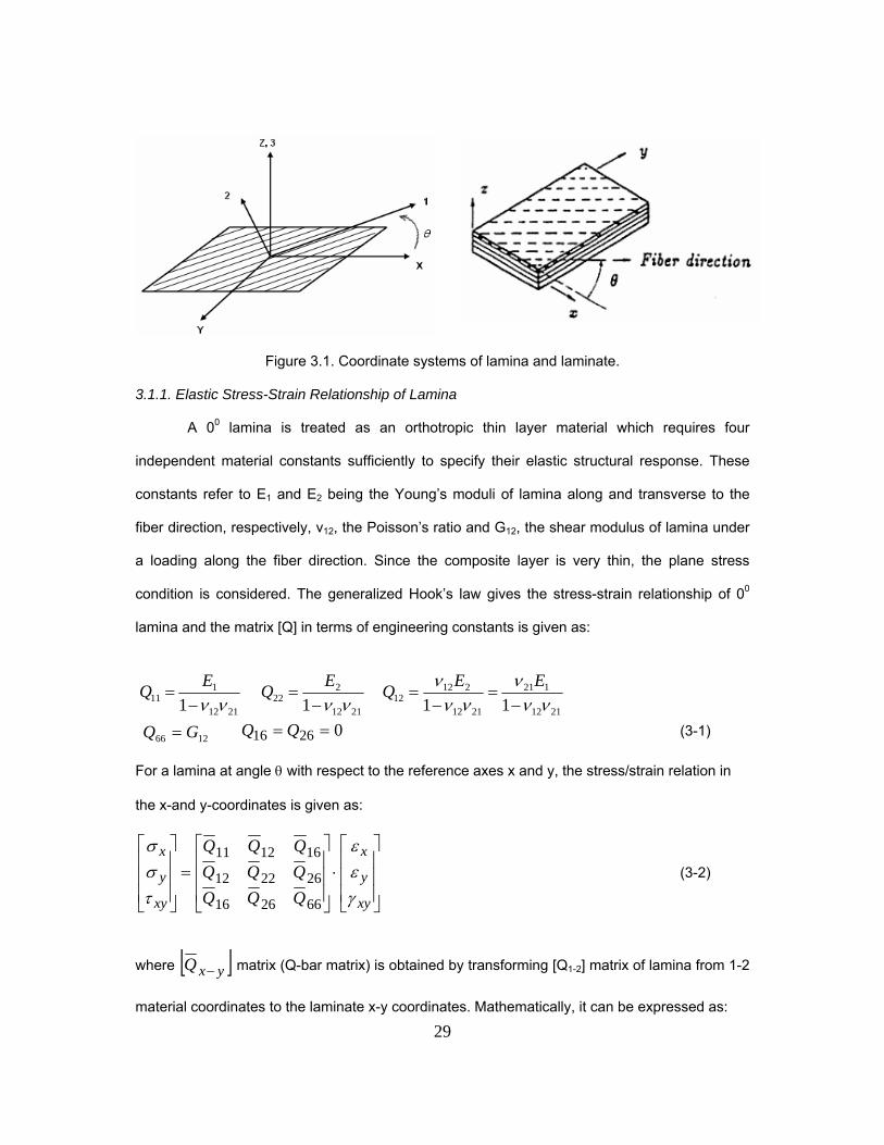
Figure 3.1. Coordinate systems of lamina and laminate.

3.1.1. Elastic Stress-Strain Relationship of Lamina

A 00 lamina is treated as an orthotropic thin layer material which requires four

independent material constants sufficiently to specify their elastic structural response. These

constants refer to E1 and E2 being the Young’s moduli of lamina along and transverse to the

fiber direction, respectively, ν12, the Poisson’s ratio and G12, the shear modulus of lamina under

a loading along the fiber direction. Since the composite layer is very thin, the plane stress

condition is considered. The generalized Hook’s law gives the stress-strain relationship of 00

lamina and the matrix [Q] in terms of engineering constants is given as:

02616 == QQ (3-1)

For a lamina at angle θ with respect to the reference axes x and y, the stress/strain relation in

the x-and y-coordinates is given as:

⎥⎥⎥

⎦

⎤

⎢⎢⎢

⎣

⎡

⋅⎥⎥⎥

⎦

⎤

⎢⎢⎢

⎣

⎡

=⎥⎥⎥

⎦

⎤

⎢⎢⎢

⎣

⎡

xy

y

x

xy

y

x

QQQQQQQQQ

γεε

τσσ

662616

262212

161211 (3-2)

where [ ]yxQ − matrix (Q-bar matrix) is obtained by transforming [Q1-2] matrix of lamina from 1-2

material coordinates to the laminate x-y coordinates. Mathematically, it can be expressed as:

2112

111 1 νν−=

EQ2112

222 1 νν−=

EQ2112

121

2112

21212 11 νν

ννν

ν−

=−

=EEQ

1266 GQ =

30

[ ] ( )[ ] [ ] ( )[ ]θθ εσ TQTQ yx ⋅⋅−= −− 21 (3-3)

[Tσ(+θ)] and [Tε(+θ)] are the transformation matrices that relate the stress and strain

components in x-y coordinates to the 1-2 coordinates, respectively. They are defined as where

m=cosθ, n= sinθ and θ is the fiber orientation of the lamina [11].

( )[ ]( )⎥

⎥⎥

⎦

⎤

⎢⎢⎢

⎣

⎡

−−−=

22

22

22

22

nmmnmnmnmn

mnnmT θσ and ( )[ ]

( )⎥⎥⎥

⎦

⎤

⎢⎢⎢

⎣

⎡

−−−=

22

22

22

22 nmmnmnmnmn

mnnmT θε (3-4)

Substituting equations 3.4 and 3.1 into 3.3, the components of the Q-bar matrix can be explicitly

expressed as:

( )661222

224

114

11 22 QQnmQnQmQ +++=

( ) ( ) 1244

66221122

12 4 QnmQQQnmQ ++−+=

( )661222

224

114

22 22 QQnmQmQnQ +++= (3-5) Strains at any point in the kth ply of a laminate can be calculated using the following relationship:

⎥⎥⎥

⎦

⎤

⎢⎢⎢

⎣

⎡

⋅+⎥⎥⎥

⎦

⎤

⎢⎢⎢

⎣

⎡

=⎥⎥⎥

⎦

⎤

⎢⎢⎢

⎣

⎡

xy

y

x

k

xy

y

x

kxy

y

x

kkk

z0

0

0

γεε

γεε

(3-6)

where εx

0, εy

0 and γxy

0 are the mid-plane strains, and κx, κy and κxy are the mid-plane curvatures.

zk is the z- coordinate of the interested point within the kth layer measured from the mid-plane to

the lamina and εx, εy and γxy are the strains in the kth ply.

)2()2( 6612223

6612113

16 QQQmnQQQnmQ −−−−−=

)2()2( 6612223

6612113

26 QQQnmQQQmnQ −−−−−=

6644

6612221122

66 )()22( QnmQQQQnmQ ++−−+=

31

3.1.2. Constitutive Equation of Laminate (Lamination Theory)

The structural response of a laminate is represented by the strains and curvatures

about its mid-plane. The total in-plane forces [ ]N and moments [ ]M per unit width of the

laminated plate are obtained by integrating forces of each ply through the laminate thickness as

shown in Figure 3.2. Mathematically, they are expressed as:

∑ ∫=

− ⎥⎥⎥

⎦

⎤

⎢⎢⎢

⎣

⎡

=⎥⎥⎥

⎦

⎤

⎢⎢⎢

⎣

⎡n

k

z

zkxy

y

x

xy

y

x k

k

dzNNN

11 τσσ

and ∑ ∫=

−

⋅⎥⎥⎥

⎦

⎤

⎢⎢⎢

⎣

⎡

=⎥⎥⎥

⎦

⎤

⎢⎢⎢

⎣

⎡n

k

z

zkxy

y

x

xy

y

x k

k

zdzMMM

11 τσσ

(3-7)

where zk-1and zk are the distances from the reference plane (often chosen at the mid-plane of

the laminate, as shown in Figure 3.3) to the kth-layer’s lower and upper surfaces, respectively.

Figure 3.2. Element of single layer with force and moment resultants.

32

Figure 3.3. Laminate plate geometry and layer numbering system.

Substituting Equations 3.2, 3.6 into 3.7, the general load-deformation relation of laminate can be

written in terms of the mid-plane strain and curvature as shown below:

⎥⎦

⎤⎢⎣

⎡⋅⎥

⎦

⎤⎢⎣

⎡=⎥

⎦

⎤⎢⎣

⎡κε 0

DBBA

MN

(3-8)

The [A], [B] and [D] matrices are given as (3-9)

where zk-1 and zk are the z-coordinates of the bottom and upper surfaces of the kth layer,

respectively. The matrix [ ]kyxQ − is the stiffness matrix of kth layer.

∑=

−− −=n

kkkkyx zzQB

1

21

2 )(][21][

∑=

−− −=n

kkkkyx zzQD

1

31

3 )(][31][

∑=

−− −=n

kkkkyx zzQA

11 )(][][

33

The [A] matrix is called in-plane extensional stiffness matrix because it directly relates the in-

plane strains ( 000 ,, xyyx γεε ) to the in-plane forces per unit width ( xyyx NNN ,, ). The [B] matrix is

called extensional-bending coupling stiffness matrix. This matrix relates the in-plane strains to

the bending moments and curvatures to in-plane forces. The [D] matrix is the bending stiffness

matrix because it relates the curvatures ( xyyx KKK ,, ) to the bending moments per unit width

( xyyx MMM ,, ).

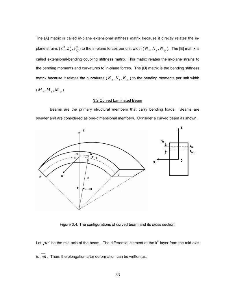
3.2 Curved Laminated Beam

Beams are the primary structural members that carry bending loads. Beams are

slender and are considered as one-dimensional members. Consider a curved beam as shown.

Figure 3.4. The configurations of curved beam and its cross section.

Let 'ρρ be the mid-axis of the beam. The differential element at the kth layer from the mid-axis

is ___mn . Then, the elongation after deformation can be written as:

Zk

Zk-1

Z

X 0

hk

Zk

Zk-1

Z

X 0

hk

Zk

Zk-1

Z

X 0

hk

Zk

Zk-1

Z

X 0

Zk

Zk-1

Z

X 0

hk

34

( ) θεθ ⋅+ dzR (3-10)

This elongation can be also described in terms of the mid-plane strain 0ε and their curvature κ .

( )κεθ ⋅+⋅ zdR 0 (3-11)

Combining 3-10 and 3-11, we have:

( )κεεθ ⋅++

= zzR

R0 (3-12)

For simplicity, the stress θσ at the kth layer can be approximated by:

kkk Q ,,

__

, θθθθ εσ = (3-13)

The resultant force and moment per unit width, θN and θM are obtained as:

( )∑∫ ∑∫= =− −

⋅++

==n

k

h

h

n

k

h

h kkk

k

k

k

dzkzzR

RQdzN1 1

0,

__

,1 1

εσ θθθθ

θθθθθ ε kBA += 0 (3-14)

∑∫=

+=⋅=−

n

k

h

h k kDBdzzM k

k10,

1θθθθθθθ εσ (3-15)

where,

∑ ∫= − +

⋅=

n

k

z

zkk

k zRdzRQA

1,

__

1θθθθ

∑ ∫= − +

⋅=

n

k

z

zkk

k zRzdzRQB

1,

__

1θθθθ

∑ ∫= − +

⋅=

n

k

z

zkk

k zRdzzRQD

1

2

,

__

1θθθθ

Explicitly,

∑= −+

+=

n

k k

kk zR

zRQRA

1 1,

__lnθθθθ (3-16)

35

( )∑= −

− ⎥⎦

⎤⎢⎣

⎡++

⋅−−=n

k k

kkkk zR

zRRzzQRB

1 11,

__

lnθθθθ (3-17)

( ) ( )∑= −

−− ⎥⎦

⎤⎢⎣

⎡⎟⎟⎠

⎞⎜⎜⎝

⎛++

+−−−=n

k k

kkkkkk zR

zRRzzRzzQRD

1 1

21

21

2,

__

ln21

θθθθ (3-18)

Combining Equations 3-14 and 3-15, we have:

⎥⎦

⎤⎢⎣

⎡⎥⎦

⎤⎢⎣

⎡=⎥

⎦

⎤⎢⎣

⎡

θθθθθ

θθθθ

θθ

θθ

κε 0

DBBA

MN

or ⎥⎦

⎤⎢⎣

⎡⋅⎥

⎦

⎤⎢⎣

⎡=⎥

⎦

⎤⎢⎣

⎡−

θθ

θθ

θθθθ

θθθθ

θκε

MN

DBBA 1

0 (3-19)

Since θθM is the only load applied to the laminated curved beam, Equation 3-19 can be re-

written as:

Δ

−= θθθθε

B; and

Δ= θθ

θθA

M

where 2θθθθθθ BDA −=Δ

θθA , θθB and θθD are referring to the extensional, coupling and bending stiffness along the θ

direction, respectively. They are equivalent to 22A , 22B and 22D for the plate laminate as the

mid-plane curvature R approaches to∞ . This is proved and shown in Appendix B. It is also

noted that θθB is not equal zero even if the laminate is symmetric with respect to its mid-plane.

With the values of 0ε and θκ , the in-plane stress θσ at any given position can be obtained from

Equations 3-12 and 3-13.

35

CHAPTER 4

STRESS EFFECT OF CURVATURE AND STACKING SEQUENCE

This Chapter discusses the tangential and radial stresses due to the variation of the

laminate curvature. The characteristics of the axial, bending and their coupling stiffness of the

curved beam are also investigated.

4.1 The Curvature Effect on Laminate Stresses

Three curved beam models with the difference in geometry dimensions were examined.

The meshing, number of elements, boundary conditions, and loading conditions remained the

same as defined in Chapter 2. Four local coordinate systems were assigned to each element

group. Each of these four local coordinate systems was associated to a different angle of fiber

orientation: 00, -450, +450, and 900, as shown in Figure 2.4. The T300/977-2 graphite/epoxy

laminate with stacking sequence of [+45/-45/902/02]S, quasi-orthotropic material, was used for

these three models. The required material properties for NASTRAN MAT9 Card are shown in

Table 2.4.

4.1.1 Stress Distribution

Model I with the mid-plane curvature of R1 = 0.2444 inches was examined and analyzed

in PATRAN/NASTRAN. The geometrical dimensions of this Model I are shown in Table 2.1.

Four plies (00 ply#6, -450 ply#2, +450 ply#1 & and 900 ply#4) from the lower half and four plies

from the upper half (00 ply#7, -450 ply#11, +450 ply#12, and 900 ply#9) of analyzed model were

selected to show different stresses distributions. The ply in the model and its sequence are

shown below.

36

Table 4.1. Ply sequence for 12-ply composite curved beam.

Ply # Orientation

1 +450 2 -450 3 900 4 900 5 00 6 00

Mid-Plane 7 00 8 00 9 900 10 900 11 -450 12 +450

Figure 4.1. The lay-up sequence of composite curved beam.

The stress distributions of eight selected plies are shown in the figures over the next pages.

37

4.1.1.1 Stress Distribution for 00 ply

Figures 4.2 and 4.3 show the tangential and radial stress contours of ply #6 and #7. As

shown, the higher stress is located at the vicinity of both free edges of the curved and straight

sides. Both tangential and radial stresses are somewhat uniform at the place away from the

free edges.

Figure 4.2. The distribution of tangential stress σθ in 00 ply.

Figure 4.3. The distribution of radial stress σr in 00 ply.

Radial stress σr of ply #6 Radial stress σr of ply #7 Radial stress σr of ply #6 Radial stress σr of ply #7

Tangential stress σθ of ply #6 Tangential stress σθ of ply #7Tangential stress σθ of ply #6 Tangential stress σθ of ply #7Tangential stress σθ of ply #6 Tangential stress σθ of ply #7

Radial stress σr of ply #6 Radial stress σr of ply #7

38

4.1.1.2 Stress Distribution for -450 ply and +450 ply

The σθ and σr stress contours are plotted in Figures 4.4 and 4.5 for -450 ply and Figures

4.6 and 4.7 for +450 ply. Comparing σθ of plies #1 and #2, the maximum magnitude occurs

along its fiber direction. The radial stress seems to be not significantly affected by the positive

or negative fiber direction.

Figure 4.4. The distribution of tangential stress σθ in -450 ply.

Figure 4.5. The distribution of radial stress σr in -450 ply.

Tangential stress σθ of ply #11 Tangential stress σθ of ply #2 Tangential stress σθ of ply #11 Tangential stress σθ of ply #2

Radial stress σr of ply #2 Radial stress σr of ply #11 Radial stress σr of ply #2 Radial stress σr of ply #11 Radial stress σr of ply #11

Tangential stress σθ of ply #2 Tangential stress σθ of ply #11

Radial stress σr of ply #2

39

Figure 4.6. The distribution of tangential stress σθ in +450 ply.

Figure 4.7. The distribution of radial stress σr in +450 ply.

Tangential stress σθ of ply #1 Tangential stress σθ of ply #12Tangential stress σθ of ply #1 Tangential stress σθ of ply #12




40

4.1.1.3 Stress Distribution for 900 ply

Since the moment is applied in the θ direction, 900 ply is the major load carrying ply of

the laminate in this case. Figures 4.8 and 4.9 show the tangential and the radial stress contours

of ply # 4 and ply #9, respectively. σθ is the highest stress component among all the plies in the

laminate. If there is no curvature in the laminate, σθ in ply #4 and #9 should be equal in

magnitude but opposite sign because of symmetrical laminate. However, this is not the case for

the curved laminate. As shown, σθ in ply #4 is larger than σθ in ply #9.

Figure 4.8. The distribution of tangential stress σθ in 900 ply.

Figure 4.9. The distribution of radial stress σr in 900 ply.

Tangential stress σθ of ply #9 Tangential stress σθ of ply #4 Tangential stress σθ of ply #9 Tangential stress σθ of ply #4




41

4.1.2 Stress Comparison

Curved beam Model I, Model II and Model III with three different mid-plane curvatures

were examined and analyzed using PATRAN/NASTRAN. The geometrical dimensions of these

three models are shown in Table 2.1. Four different plies (00 ply#6, -450 ply#2, +450 ply#1 &

and 900 ply#4) from the lower half of these models were selected for stress comparison.

Twenty different elements which associated with twenty different angle positions from each ply,

as shown in Figure 4.10, were selected to eliminate the “edge effective”.

Figure 4.10. Elements on each ply at different angle position.

The values of radial stress rσ and tangential stress θσ for these twenty elements were

recorded from the PATRAN/NASTRAN output. These stress values were then plotted into

different graphs. Each of these graphs shows the stress variation of each individual ply at a

different angle of fiber orientation from three different analyzed curved beam models. The

behavior and the variation of interlaminar stresses from each different layer due to the changing

in curvature of each model highlighted clearly from these graphs.

Twenty selected elements

42

4.1.2.1 The Stress Variation for +450 ply#1

Table 4.2. The stress values for +450 ply#1.

(deg) Model I (R1 = 0.2444) Model II (R2 = 0.6444) Model III (R3 = 1.8444) Angle

Position

σr (psi)

σθ (psi)

σr (psi)

σθ (psi)

σr (psi)

σθ (psi)

30 5.11E+02 5.48E+04 4.70E+02 4.74E+04 1.43E+02 4.50E+0427 5.13E+02 5.49E+04 4.61E+02 4.72E+04 1.44E+02 4.50E+0424 5.14E+02 5.50E+04 4.64E+02 4.70E+04 1.46E+02 4.51E+0421 5.15E+02 5.50E+04 4.60E+02 4.69E+04 1.41E+02 4.52E+0418 5.16E+02 5.51E+04 4.60E+02 4.67E+04 1.49E+02 4.54E+0415 5.16E+02 5.51E+04 4.59E+02 4.66E+04 1.46E+02 4.55E+0412 5.16E+02 5.51E+04 4.59E+02 4.66E+04 1.37E+02 4.55E+049 5.16E+02 5.52E+04 4.58E+02 4.65E+04 1.50E+02 4.56E+046 5.17E+02 5.52E+04 4.59E+02 4.65E+04 1.40E+02 4.56E+043 5.17E+02 5.52E+04 4.58E+02 4.65E+04 1.54E+02 4.57E+04-3 5.17E+02 5.52E+04 4.58E+02 4.65E+04 1.32E+02 4.57E+04-6 5.18E+02 5.53E+04 4.59E+02 4.65E+04 1.51E+02 4.57E+04-9 5.18E+02 5.53E+04 4.58E+02 4.66E+04 1.46E+02 4.57E+04

-12 5.19E+02 5.54E+04 4.60E+02 4.66E+04 1.41E+02 4.57E+04-15 5.20E+02 5.54E+04 4.59E+02 4.67E+04 1.45E+02 4.56E+04-18 5.21E+02 5.55E+04 4.62E+02 4.68E+04 1.52E+02 4.56E+04-21 5.22E+02 5.57E+04 4.60E+02 4.70E+04 1.34E+02 4.55E+04-24 5.25E+02 5.59E+04 4.66E+02 4.71E+04 1.57E+02 4.56E+04-27 5.28E+02 5.62E+04 4.61E+02 4.73E+04 1.34E+02 4.55E+04-30 5.31E+02 5.65E+04 4.75E+02 4.76E+04 1.59E+02 4.57E+04

The tangential stress θσ and radial stress rσ are found to be positive for +450 lay-up #1, as

shown in Figure 4.11 and Figure 4.12 on the next page. As expected, the stresses θσ and

rσ along the curve angle position are fairly constant. However, these stresses decrease with

the increasing of curvatures. Figure 4.12 clearly highlights the effect of curvature on radial

stress rσ . Model I (R1 = 0.2444) with the lowest in radius of curvature produces the highest in

interlaminar stresses. On the other hand, Model III (R3 = 1.8444) with the highest in radius of

curvature produces the lowest in interlaminar stresses.

43

The Variation of Tangential Stress for +45deg Lay-up

0.00E+00

1.00E+04

2.00E+04

3.00E+04

4.00E+04

5.00E+04

6.00E+04

-40 -30 -20 -10 0 10 20 30 40

Angle Position

Tang

entia

l Str

ess Curvature_R1

Curvature_R2

Curvature_R3

Figure 4.11. Tangential stress for +450 lay-up.

The Variation of Radial Stress for +45deg Lay-up

0.00E+00

1.00E+02

2.00E+02

3.00E+02

4.00E+02

5.00E+02

6.00E+02

-40 -30 -20 -10 0 10 20 30 40

Angle Position

Rad

ial S

tres

s

Curvature_R1

Curvature_R2

Curvature_R3

Figure 4.12. Radial stress for +450 lay-up.

44

4.1.2.2 The Stress Variation for -450 ply#2

Table 4.3. The stress values for -450 ply#2.


Position

σr (psi)

σθ (psi)

σr (psi)

σθ (psi)

σr (psi)

σθ (psi)



The tangential stress θσ and radial stress rσ are found to be positive for -450 lay-up #2, as

shown in Figure 4.13 and Figure 4.14 on the next page. For this -450 lay-up, the tangential

stress θσ increases with the increasing of curvature. The radial stress rσ decreases with the

increasing of curvature. Model I (R1 = 0.2444) with the lowest in radius of curvature produces

the highest in radial stress and lowest in tangential stress. On the other hand, Model III (R3

=1.8444) with the highest in curvature produces the lowest in radial stress and highest

tangential stress.

45

The Variation of Tangential Stress for -45deg Lay-up

2.80E+04

4.20E+04

5.60E+04

-40 -30 -20 -10 0 10 20 30 40

Angle Position

Tang

entia

l Str

ess

Curvature_R1

Curvature_R2

Curvature_R3

Figure 4.13. Tangential stress for -450 lay-up.

The Variation of Radial Stress for -45deg Lay-up

0.00E+00

5.00E+02

1.00E+03

1.50E+03

2.00E+03

2.50E+03

3.00E+03

3.50E+03

-40 -30 -20 -10 0 10 20 30 40

Angle Position

Rad

ial S

tres

s

Curvature_R1

Curvature_R2

Curvature_R3

Figure 4.14. Radial stress for -450 lay-up.

46

4.1.2.3 The Stress Variation for 900 ply#4

Table 4.4. The stress values for 900 ply#4.


Position

σr (psi)

σθ (psi)

σr (psi)

σθ (psi)

σr (psi)

σθ (psi)



The tangential stress θσ and radial stress rσ are found to be positive for 900 lay-up #4, as

shown in Figure 4.15 and Figure 4.16 on the next page. For this 900 lay-up, the tangential

stress θσ increases with the increasing of curvature. The radial stress rσ decreases with the

increasing of curvature. Model I (R1 = 0.2444) with the lowest in radius of curvature produces

the highest in radial stress and lowest in tangential stress. On the other hand, Model III (R3 =

1.8444) with the highest in radius of curvature produces the lowest in radial stress and highest

tangential stress.

47

The Variation of Tangential Stress for 90deg Lay-up

0.00E+00

1.00E+04

2.00E+04

3.00E+04

4.00E+04

5.00E+04

6.00E+04

7.00E+04

8.00E+04

9.00E+04

1.00E+05

-40 -30 -20 -10 0 10 20 30 40

Angle Position

Tang

entia

l Str

ess

Curvature_R1

Curvature_R2

Curvature_R3

Figure 4.15. Tangential stress for 900 lay-up.

The Variation of Radial Stress for 90deg Lay-up

0.00E+00

1.00E+03

2.00E+03

3.00E+03

4.00E+03

5.00E+03

6.00E+03

7.00E+03

8.00E+03

9.00E+03

-40 -30 -20 -10 0 10 20 30 40

Angle Position

Rad

ial S

tres

s

Curvature_R1

Curvature_R2

Curvature_R3

Figure 4.16. Radial stress for 900 lay-up.

48

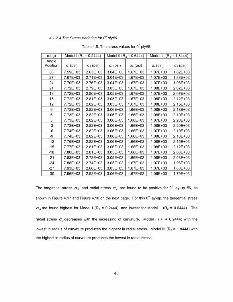
4.1.2.4 The Stress Variation for 00 ply#6

Table 4.5. The stress values for 00 ply#6.


Position

σr (psi)

σθ (psi)

σr (psi)

σθ (psi)

σr (psi)

σθ (psi)



The tangential stress θσ and radial stress rσ are found to be positive for 00 lay-up #6, as

shown in Figure 4.17 and Figure 4.18 on the next page. For this 00 lay-up, the tangential stress

θσ are found highest for Model I (R1 = 0.2444), and lowest for Model II (R2 = 0.6444). The

radial stress rσ decreases with the increasing of curvature. Model I (R1 = 0.2444) with the

lowest in radius of curvature produces the highest in radial stress. Model III (R3 = 1.8444) with

the highest in radius of curvature produces the lowest in radial stress.

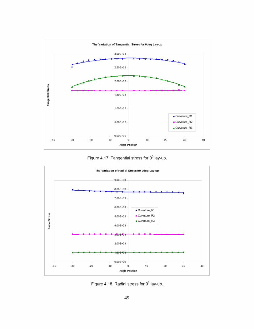
49

The Variation of Tangential Stress for 0deg Lay-up

0.00E+00

5.00E+02

1.00E+03

1.50E+03

2.00E+03

2.50E+03

3.00E+03

-40 -30 -20 -10 0 10 20 30 40

Angle Position

Tang

entia

l Str

ess

Curvature_R1

Curvature_R2

Curvature_R3

Figure 4.17. Tangential stress for 00 lay-up.

The Variation of Radial Stress for 0deg Lay-up

0.00E+00

1.00E+03

2.00E+03

3.00E+03

4.00E+03

5.00E+03

6.00E+03

7.00E+03

8.00E+03

9.00E+03

-40 -30 -20 -10 0 10 20 30 40

Angle Position

Rad

ial S

tres

s

Curvature_R1

Curvature_R2

Curvature_R3

Figure 4.18. Radial stress for 00 lay-up.

50

4.1.3 Stacking Sequence [+450/-450/9002/00

2]S

The tangential stresses along the θ direction of -450 (ply#2), +450 (ply #1) and 900 (ply

#4) are calculated using the closed-form solution in Chapter 3. These calculated stress values

are used to validate the obtained tangential stress values in Section 4.1.2. The comparison

between FEM and the closed-form solution is shown in Table 4.6.

Table 4.6. The comparison for tangential stress.

Applied bending moment Mθθ = 100 lbs-in Tangential stress, σθθ (psi)

R1 = 0.2444 inches R2 = 0.6444 inches R3 = 1.8444 inches

FEM Present FEM Present FEM Present -450 Ply 4.09E+04 4.20E+04 4.37E+04 4.03E+04 4.45E+04 3.97E+04 +450 Ply 5.52E+04 5.36E+04 4.65E+04 4.97E+04 4.57E+04 4.83E+04 900 Ply 5.07E+04 5.21E+04 6.28E+04 5.64E+04 8.58E+04 7.13E+04

% Different % Different % Different -450 Ply 2.62 8.44 12.09 +450 Ply 2.99 6.44 5.38 900 Ply 2.69 11.35 20.34

The difference in tangential stress between the FEM result and the closed-form solution is

predictable. This difference takes place due to the fact that the FEM includes 3D material

properties while the closed-form solution includes only 1D material property.

51

4.2 The Fiber Orientation Effect on Laminate Stresses

The effect of fiber orientation is also investigated. Model I (R1 = 0.2444) was examined.

The meshing, the number of elements, boundary conditions and material coordinate systems for

this model were remained the same as defined in Sections 2.1 and 2.2.

4.2.1 Symmetric and Balanced Laminates

A T300/977-2 graphite/epoxy laminate with stacking sequence of [ θ± / θ± / 9002]S was

used for the selected models, where =θ 150, 300, 450, 600, and 750. A different local

coordinate was created for each different angle of fiber orientation: 00, +150, -150, +300, -300,

+450, -450, +600, -600, +750, and -750. There are five different stacking sequences were applied

for this model. They are: [ 015± / 015± / 9002]S, [ 030± / 030± / 900

2]S, [ 045± / 045± / 9002]S,

[ 060± / 060± / 9002]S, and [ 075± / 075± / 900

2]S.

S.S #1 S.S #2 S.S #3 S.S #4 S.S #5 +150 +300 +450 +600 +750 -150 -300 -450 -600 -750 +150 +300 +450 +600 +750 -150 -300 -450 -600 -750 900 900 900 900 900 900 900 900 900 900 900 900 900 900 900 900 900 900 900 900 -150 -300 -450 -600 -750 +150 +300 +450 +600 +750 -150 -300 -450 -600 -750 +150 +300 +450 +600 +750

Figure 4.19. Description of laminate coding for five different stacking sequences.

The interlaminar stresses for the elements in 900 layer are expected to be different for each

stacking sequence. To study the effect of changing in stacking sequence, three different

elements in the 900 layer #6 from the lower half of the curved beam model were examined.

52

These three elements were selected from three different angle positions (270, 330 and 390), as

shown in Figure 4.20. The element at 450 angle position was not selected for this case study

since the result at this position may be strongly affected by the end condition enforced by FEM.

Figure 4.20. The selected elements in 900 layer #6 at different angle positions.

The variation of θσ and rσ stresses for the selected elements in 900 layer #6 at various angle

positions (270, 330, and 390) are shown below for five different stacking sequences.

Color Codes

Figure 4.21. Stress for element at 270 angle position.

Element at 27deg angle position.

0.00E+00

2.00E+03

4.00E+03

6.00E+03

8.00E+03

1.00E+04

1.20E+04

27

Angle Position, deg

Rad

ial S

tres

s, p

si

S.S #1

S.S #2

S.S #3

S.S #4

S.S #5


-6.00E+03

-4.00E+03

-2.00E+03

0.00E+00

2.00E+03

4.00E+03

6.00E+03

8.00E+03

1.00E+04

1.20E+04

1.40E+04

27

Angle Position, deg

Tang

entia

l Str

ess,

psi

S.S #1

S.S #2

S.S #3

S.S #4

S.S #5


0.00E+00

2.00E+03

4.00E+03

6.00E+03

8.00E+03

1.00E+04

1.20E+04

27

Angle Position, deg

Rad

ial S

tres

s, p

si

S.S #1

S.S #2

S.S #3

S.S #4

S.S #5


-6.00E+03

-4.00E+03

-2.00E+03

0.00E+00

2.00E+03

4.00E+03

6.00E+03

8.00E+03

1.00E+04

1.20E+04

1.40E+04

27

Angle Position, deg

Tang

entia

l Str

ess,

psi

S.S #1

S.S #2

S.S #3

S.S #4

S.S #5

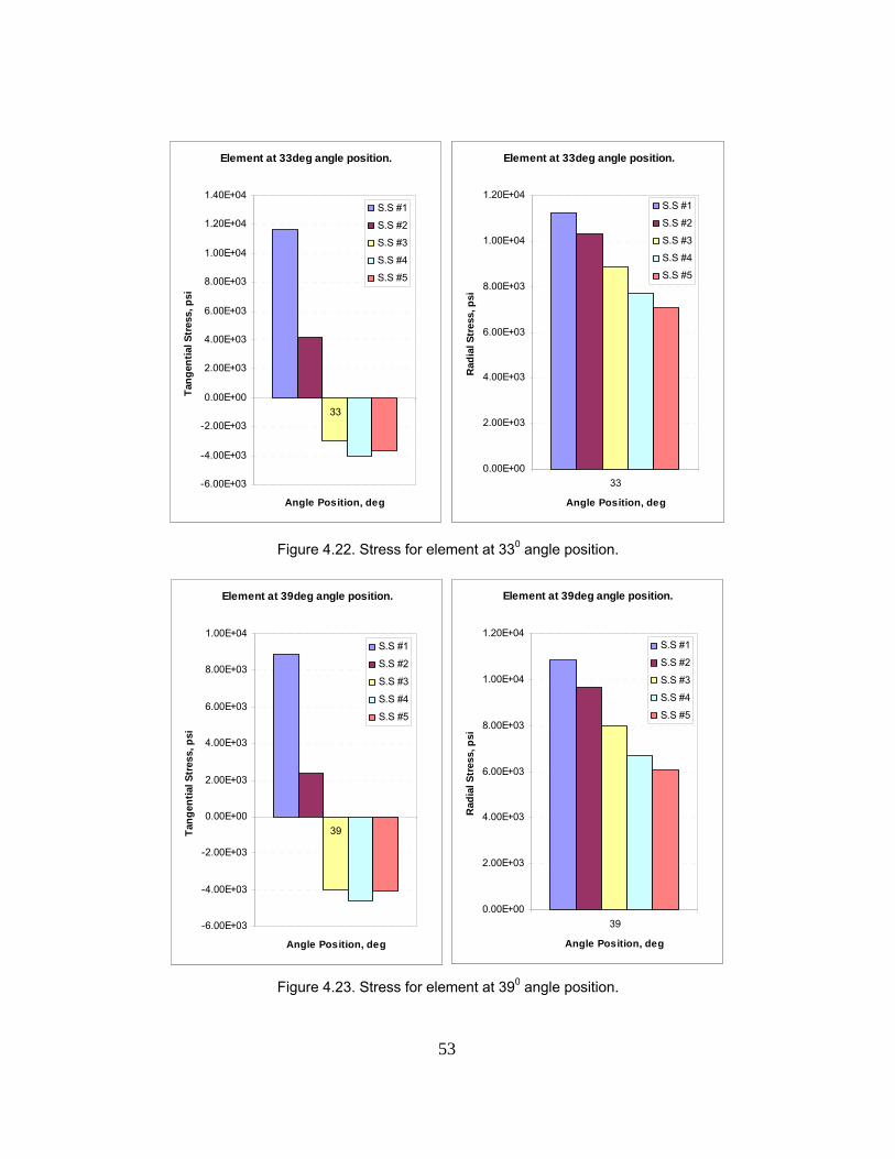
53




0.00E+00

2.00E+03

4.00E+03

6.00E+03

8.00E+03

1.00E+04

1.20E+04

33

Angle Position, deg

Rad

ial S

tres

s, p

si

S.S #1

S.S #2

S.S #3

S.S #4

S.S #5


-6.00E+03

-4.00E+03

-2.00E+03

0.00E+00

2.00E+03

4.00E+03

6.00E+03

8.00E+03

1.00E+04

1.20E+04

1.40E+04

33

Angle Position, deg

Tang

entia

l Str

ess,

psi

S.S #1

S.S #2

S.S #3

S.S #4

S.S #5


0.00E+00

2.00E+03

4.00E+03

6.00E+03

8.00E+03

1.00E+04

1.20E+04

33

Angle Position, deg

Rad

ial S

tres

s, p

si

S.S #1

S.S #2

S.S #3

S.S #4

S.S #5


-6.00E+03

-4.00E+03

-2.00E+03

0.00E+00

2.00E+03

4.00E+03

6.00E+03

8.00E+03

1.00E+04

1.20E+04

1.40E+04

33

Angle Position, deg

Tang

entia

l Str

ess,

psi

S.S #1

S.S #2

S.S #3

S.S #4

S.S #5


-6.00E+03

-4.00E+03

-2.00E+03

0.00E+00

2.00E+03

4.00E+03

6.00E+03

8.00E+03

1.00E+04

39

Angle Position, deg

Tang

entia

l Str

ess,

psi

S.S #1

S.S #2

S.S #3

S.S #4

S.S #5


0.00E+00

2.00E+03

4.00E+03

6.00E+03

8.00E+03

1.00E+04

1.20E+04

39

Angle Position, deg

Rad

ial S

tres

s, p

si

S.S #1

S.S #2

S.S #3

S.S #4

S.S #5


-6.00E+03

-4.00E+03

-2.00E+03

0.00E+00

2.00E+03

4.00E+03

6.00E+03

8.00E+03

1.00E+04

39

Angle Position, deg

Tang

entia

l Str

ess,

psi

S.S #1

S.S #2

S.S #3

S.S #4

S.S #5


0.00E+00

2.00E+03

4.00E+03

6.00E+03

8.00E+03

1.00E+04

1.20E+04

39

Angle Position, deg

Rad

ial S

tres

s, p

si

S.S #1

S.S #2

S.S #3

S.S #4

S.S #5

54

Figures 4.21, 4.22 and 4.23 highlight clearly the effect of fiber orientations on the interlaminar

stresses ( θσ and rσ ). The radial stress rσ is found positive for all stacking sequences at all

selected angle positions. The stacking sequences #1 & #2 produced positive tangential stress

θσ and the stacking sequences #3, #4, & #5 produced negative tangential stress θσ at all

selected angle positions. This is because of the shift of the neutral axis of the curved laminate

as the fiber orientation changes. The stacking sequence #1, [ 015± / 015± / 9002]S, produced

the highest interlaminar stresses ( θσ and rσ ) for elements in 900 layer #6.

4.2.2 Symmetric / Unsymmetrical and Balanced / Unbalanced Laminates

The effects of three other stacking sequences on the tangential stress were also

investigated. The symmetric and balanced laminate [ ]T20

40

20 45/90/45 m± , unsymmetrical

and balanced laminate [ ]T40

20

20 90/45/45 ±± , and unsymmetrical and unbalanced laminate

[ ]T40

80 90/45+ were applied in the same Model I (R1 = 0.2444). The layer #1 of +450 fiber

orientation was selected to show the different in tangential stress. The stacking sequences are

shown below.

S.S #1 S.S #2 S.S #3 +450 +450 +450 -450 -450 +450 +450 +450 +450 -450 -450 +450 900 +450 +450 900 -450 +450 900 +450 +450 900 -450 +450 -450 900 900 +450 900 900 -450 900 900 +450 900 900

Figure 4.24. Description of laminate coding for three different stacking sequences.

55

Twenty different elements which associated with twenty different angle positions, as shown in

Figure 4.10, were selected for this study. The tangential stresses from three different stacking

sequences were plotted in the same graph for comparison purposes.

Tangential Stress, +45 deg Ply, Layer #1

0.00E+00

1.00E+04

2.00E+04

3.00E+04

4.00E+04

5.00E+04

6.00E+04

7.00E+04

8.00E+04

9.00E+04

-40 -30 -20 -10 0 10 20 30 40Angle position, deg

Tang

entia

l stre

ss, p

si

Layup_01Layup_02Layup_03

Figure 4.25. The variation of tangential stress.

The tangential stress θσ was found positive for all stacking sequences. The symmetric and

balanced laminate [ ]T20

40

20 45/90/45 m± produced the highest tangential stress for +450

layer #1. The unsymmetrical and balanced laminate [ ]T40

20

20 90/45/45 ±± produced the

lowest tangential stress for +450 layer #1.

56

4.3 The Effect of Stacking Sequence

Five different laminates were examined to show the effect of the lay-up stacking

sequences on the extensional stiffness matrix [A], extensional-bending coupling stiffness matrix

[B], and bending stiffness matrix [D]. These five laminates and their lay-up stacking sequences

are shown in Table 4.7 below.

Table 4.7. Laminate stacking sequences.

LAMINATE 1 [00/00/+450/-450/900/900]S Symmetric and Balanced LAMINATE 2 [+450/00/00/-450/900/900]S Symmetric and Balanced LAMINATE 3 [+450/-450/00/00/900/900]S Symmetric and Balanced LAMINATE 4 [+450/-450/900/900/00/00]S Symmetric and Balanced LAMINATE 5 [+450

2/-4502/00

4/9004]T Unsymmetrical and Balanced

The calculated values of matrices θθA , θθB , and θθD using Equations 3-16, 3-17, and 3-18

with different laminate stacking sequences and/or different mid-plane radius R are shown in the

following table.

Table 4.8. Matrices comparison for laminate 3.

R1 = 0.2444 R2 = 0.6444 R3 = 1.8444 R ∞ Aθθ (105

lb/in) 9.055 9.002 8.995 8.994 Bθθ (102 lb) -14.88 -5.54 -1.93 0.00

Dθθ (102 lb-in) 3.64 3.57 3.56 3.56

As indicated in Table 4.8, θθA and θθD fairly remain constant as R increases. However, the

magnitude of θθB strongly decreases as R increases. The values of matrices θθA , θθB and

θθD are then re-evaluated with four different laminates (1, 2, 3, and 4) and one mid-plane

radius, R = 0.2444 inches. These values are shown in Table 4.9. Unlike the plate laminate, the

changing of stacking sequence in the curved laminate does affect the axial stiffness, θθA .

57

It should be also noted that 0≠θθB for curved laminates as listed in Table 4.9. This Table 4.9

also indicates that increasing R gives significant reduction of θθB .

Table 4.9. Matrices comparison for mid-plane radius R1 = 0.2444 inches.

LAMINATE 1 LAMINATE 2 LAMINATE 3 LAMINATE 4 Aθθ (105

lb/in) 9.031 9.044 9.055 9.099 Bθθ (102 lb) -9.03 -12.34 -14.88 -25.74

Dθθ (102 lb-in) 2.21 3.02 3.64 6.29

The effect of symmetric and balanced laminate and unsymmetrical and balanced laminate was

also investigated. Laminate 3 and laminate 5 were examined with four mid-plane radius

R1 = 0.2444 inches, R2 = 0.6444 inches, R3 = 1.8444 inches, and R ∞. The values of

matrices θθA , θθB and θθD are shown below.

Table 4.10. Matrices comparison for laminate 3 & 5.

R1 = 0.2444 R2 = 0.6444 LAMINATE

3LAMINATE 5 LAMINATE 3 LAMINATE 5

Aθθ (105 lb/in) 9.055 8.588 9.002 8.810

Bθθ (102 lb) -14.88 99.22 -5.54 118.40 Dθθ (102 lb-in) 3.64 7.69 3.57 7.92

R3 = 1.8444 R ∞ LAMINATE

3LAMINATE 5 LAMINATE 3 LAMINATE 5

Aθθ (105 lb/in) 8.995 8.925 8.994 8.994

Bθθ (102 lb) -1.93 126.33 0.00 130.69 Dθθ (102 lb-in) 3.56 8.05 3.56 8.12

As the radius of curvature R goes to infinity, a curved laminate becomes a plate laminate. In

this case, extensional-bending coupling stiffness matrix [B] is only affected by the stacking

sequence in laminate. This indication is shown in Table 4.10. For laminate 3 (symmetric and

balanced), Bθθ is equal to zero when the radius of curvature R goes to infinity. For laminate 5

(unsymmetrical and balanced), Bθθ is not equal to zero when the radius of curvature R goes to

infinity.

58

CHAPTER 5

CONCLUSIONS AND FUTURE WORK

The research has studied the variation of both tangential and radial stresses respect to

the changing in curvatures, stacking sequences and fiber orientations in a curved laminated

beam subjected to a bending moment. Three 3-D finite element models of the curved laminated

beam have been developed in PATRAN / NASTRAN. These models have been validated for

isotropic material, Al-2014-T6, and orthotropic material, T300/977-2 graphite/epoxy, with all 00

plies lay-up. The finite element models of the curved laminated beam provide solutions

showing an excellent agreement with the exact solutions for both tangential and radial stresses.

An analytical method to calculate the tangential stress was also developed for a curved

laminated beam subjected to a bending moment. The tangential stress results from this method

were compared well with the results from finite element method. The analytical closed-form

expressions of axial, coupling and bending stiffness, as well as their characteristics were also

investigated.

From this research, the following conclusions can be made.

For the same stacking sequence, [+450/-450/9002/00

2]S with three different given radius

of curvatures:

• In +450 (layer #1, the bottom layer) and -450 (layer #2, the 2nd to the bottom),

the tangential and radial stresses increase with the decreasing in radius of

curvatures.

• In 900 (layer #4, from the bottom layer), the tangential stress decreases with the

decreasing in radius of curvature. The radial stress increases with the

decreasing in curvature.

59

• In 00 (layer #6, from the bottom), the tangential stress is highest for radius of

curvature R1 and lowest for radius of curvature R2. The radial stress increases

with the decreasing in curvature.

For a given radius of curvature with five different symmetric and balanced stacking

sequences, the stress for elements on 900 layer #6 from the bottom layer:

• The radial stress is positive for all stacking sequences.

• The tangential stresses from stacking sequence #1, [ 015± / 015± / 9002]S, and

stacking sequence #2, [ 030± / 030± / 9002]S, are positive.

• The tangential stresses from stacking sequence #3, [ 045± / 045± / 9002]S,

stacking sequence #4, [ 060± / 060± / 9002]S, and stacking sequence #5,

[ 075± / 075± / 9002]S, are negative.

• The tangential and radial stresses from stacking sequence #1, [ 015± / 015± /

9002]S, are highest.

For a given radius of curvature with three different stacking sequences:

[ ]T20

40

20 45/90/45 m± , [ ]T4

02

02

0 90/45/45 ±± , and [ ]T40

80 90/45+ , the stress for

elements on +450 layer #1, bottom layer:

• The tangential stresses θσ are positive for all stacking sequences.

• The symmetric and balanced laminate, [ ]T20

40

20 45/90/45 m± , produced the

highest tangential stress.

• The unsymmetrical and balanced laminate, [ ]T40

20

20 90/45/45 ±± ,

produced the lowest tangential stress.

60

For a symmetric and balanced laminate:

• θθA and θθD fairly remain constant as R increases.

• The magnitude of θθA is affected by the changing of stacking sequence in the

curved laminate.

• θθB is not equal to zero for curved laminated beam but its magnitude strongly

decreases as R increases.

• The increasing of radius curvature gives significant reduction of θθB .

In future studies, the developed analytical method could be extended to laminated

cylindrical shell. The hygrothermal effects on the tangential and radial stresses can be

included. Effect of stress components due to the boundary conditions and loading of the curved

beam can be investigated.

61

APPENDIX A

GENERAL PROCEDURE TO CREATE A 3D FEM FOR AN ISOTROPIC AND A CURVED LAMINATED BEAM IN PATRAN

62

Figure A1. The creation of 12 surfaces.

Figure A2. The creation of 12 solids and mesh seeds.

Original first surface

11 surfaces offset from original first surface

Ply thickness

Original first surface

11 surfaces offset from original first surface

Ply thickness

Each solid was extruded from each surface

Create mesh seeds for edges

Extrudedthickness

Each solid was extruded from each surface

Create mesh seeds for edges

Extrudedthickness

63

Figure A3. The creation for the mesh and MPC.

Create Mesh Create Multipoint ConstraintCreate Mesh Create Multipoint Constraint

64

Figure A4. The creation of local coordinates for each element group in laminate.

00 Coord 1 -450 Coord 2 450 Coord 3 900 Coord 400 Coord 1 -450 Coord 2 450 Coord 3 900 Coord 4

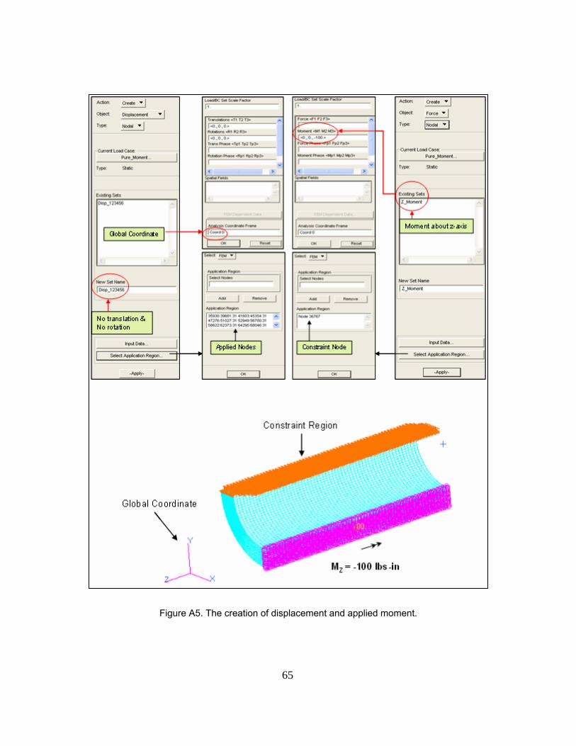
65

Figure A5. The creation of displacement and applied moment.

66

Figure A6. The creation of cylindrical coordinate system for isotropic.

Figure A7. The creation of Isotropic material and 3D solid elements.

Cylindrical coordinate system

1

1

Applied Elements

Material propertiesCylindrical coordinate system

1

1

Applied Elements

Material properties

67

Figure A8. The creation of 3D orthotropic material and 3D solid group elements.

68

Figure A9. The creation of analysis Load case.

Boundary Conditions

Load Case

Boundary Conditions

Load Case

69

Figure A10. The procedure to set up the analysis.

12

34

1

2

3

4

Request results respect to materialCoordinate system

12

34

1

2

3

4

Request results respect to materialCoordinate system

70

APPENDIX B

MATHEMATICAL PROCEDURE TO VERIFY THE ACCURACY OF MATRIX [A], [B], AND [D] WHEN THE CURVATURE GOES TO INFINITY

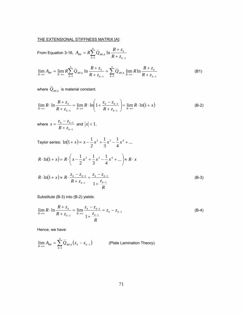
71

THE EXTENSIONAL STIFFNESS MATRIX [A]:

From Equation 3-16, ∑= −+

+=

n

k k

kk zR

zRQRA

1 1,

__lnθθθθ

∑∑= −

∞→= −

∞→∞→ ++

=++

=n

k k

k

Rk

n

k k

kkRR zR

zRRQ

zRzR

QRA1 1

,

__

1 1,

__lnlimlnlimlim θθθθθθ (B1)

where kQ ,

__

θθ is material constant.

( )xRzRzz

RzRzR

RR

k

kk

Rk

k

R+⋅=⎟⎟

⎠

⎞⎜⎜⎝

⎛+−

+⋅=++

⋅∞→

−

−

∞→−

∞→1lnlim1lnlimlnlim

1

1

1

(B-2)

where 1

1

−

−

+−

=k

kk

zRzz

x and .1<x

Taylor series: ( ) ...41

31

211ln 432 +−+−=+ xxxxx

( ) xRxxxxRxR ⋅≈⎟⎠⎞

⎜⎝⎛ +−+−⋅=+⋅ ...

41

31

211ln 432

( )

Rzzz

zRzz

RxRk

kk

k

kk

1

1

1

1

11ln

−

−

−

−

+

−=

+−

⋅≈+⋅ (B-3)

Substitute (B-3) into (B-2) yields:

11

1

1 1limlnlim −

−

−

∞→−

∞→−=

+

−=

++

⋅ kkk

kk

Rk

k

Rzz

Rzzz

zRzR

R (B-4)

Hence, we have:

( )11

,

__

lim −=

∞→−= ∑ kk

n

kkR

zzQA θθθθ (Plate Lamination Theory).

72

THE EXTENSIONAL-BENDING COUPLING STIFFNESS MATRIX [B]:

From Equation 3-17, ( )∑= −

− ⎥⎦

⎤⎢⎣

⎡++

⋅−−=n

k k

kkkk zR

zRRzzQRB

1 11,

__

lnθθθθ

( )∑= −

−∞→∞→ ⎥⎦

⎤⎢⎣

⎡++

⋅−−⋅=n

k k

kkkkRR zR

zRRzzRQB

1 1

21,

__

lnlimlim θθθθ

( ) ⎟⎟⎠

⎞⎜⎜⎝

⎛++

⋅−−⋅=−

∞→−∞→=

∞→ ∑1

21

1,

__

lnlimlimlimk

k

RkkR

n

kkR zR

zRRzzRQB θθθθ (B-5)

( )xRzRzR

RR

k

k

R+⋅=

++

⋅∞→

−∞→

1lnlimlnlim 2

1

2 , where 1

1

−

−

+−

=k

kk

zRzz

x and .1<x

( ) ( ) ⎟⎠⎞

⎜⎝⎛ ⋅−⋅≈⎟

⎠⎞

⎜⎝⎛ +−+−⋅=+⋅

∞→∞→∞→

2243222

21lim...

41

31

21lim1lnlim xRxRxxxxRxR

RRR (B-6)

( ) ( )yzzR

Rzzz

RzRzz

RxR kkRk

kk

Rk

kk

RR +−=

⎟⎟⎟⎟

⎠

⎞

⎜⎜⎜⎜

⎝

⎛

+

−⋅=

+−

⋅=⋅ −∞→−

−

∞→−

−

∞→∞→ 11lim

1limlimlim 1

1

1

1

122 (B-7)

where R

zy k 1−= and 1<y

Taylor series: ...11

1 32 +−+−=+

yyyy

for 1<y (B-8)

Substitute (B8) into (B7) yields:

( ) ⎟⎟⎠

⎞⎜⎜⎝

⎛+⎟

⎠⎞

⎜⎝⎛−⎟

⎠⎞

⎜⎝⎛+−⋅−⋅=⋅ −−−

−∞→∞→...1limlim

31

211

12

Rz

Rz

Rz

zzRxR kkkkkRR

( ) ( )1112 limlimlim −−∞→−∞→∞→

−⋅−−⋅≈⋅ kkkRkkRRzzzzzRxR

( ) ( )111lim −−−∞→−⋅−−⋅= kkkkkR

zzzzzR (B-9)

73

( ) ( )⎟⎟⎟⎟

⎠

⎞

⎜⎜⎜⎜

⎝

⎛

⎟⎟⎟⎟

⎠

⎞

⎜⎜⎜⎜

⎝

⎛

+⋅−=⎟⎟

⎠

⎞⎜⎜⎝

⎛+−

⋅=⋅

−−∞→

−

−

∞→∞→

2

1

21

2

1

12

1

1lim21lim

21

2lim

Rz

zzzRzz

RxRk

kkRk

kk

RR

Taylor series: ⎟⎟⎠

⎞⎜⎜⎝

⎛+⎟

⎠⎞

⎜⎝⎛−⎟

⎠⎞

⎜⎝⎛+−=

+

−−−

−

...11

1 31

211

1 Rz

Rz

Rz

Rz

kkk

k

Then, ( ) ( ) ( )2

12

1

2

21lim

21

2lim −−∞→∞→

−=−=⋅

kkkkRRzzzzxR

(B-10)

Equation B-6 becomes:

( ) ( ) ( )21111

1

2 lim21limlimlnlim −∞→−−∞→−∞→

−∞→

−−−⋅−−⋅=++

⋅ kkRkkkRkkRk

k

RzzzzzzzR

zRzR

R

( ) ( ) ( )12

1111

2 lim21lnlim −∞→−−−

−∞→

−⋅+−−−⋅−=++

⋅ kkRkkkkkk

k

RzzRzzzzz

zRzR

R

( ) ( )122

11

2 lim21lnlim −∞→−

−∞→

−⋅+−=++

⋅ kkRkkk

k

RzzRzz

zRzR

R (B-11)

Substitute B-11 into B-5 yields:

( ) ( ) ( )⎟⎠⎞

⎜⎝⎛ −⋅−−−−⋅= −∞→−−∞→

=∞→ ∑ 1

2211

1,

__

lim21limlim kkRkkkkR

n

kkR

zzRzzzzRQB θθθθ

( )21

2

1,

__

21lim −

=∞→

−= ∑ kk

n

kkR

zzQB θθθθ (Plate Lamination Theory).

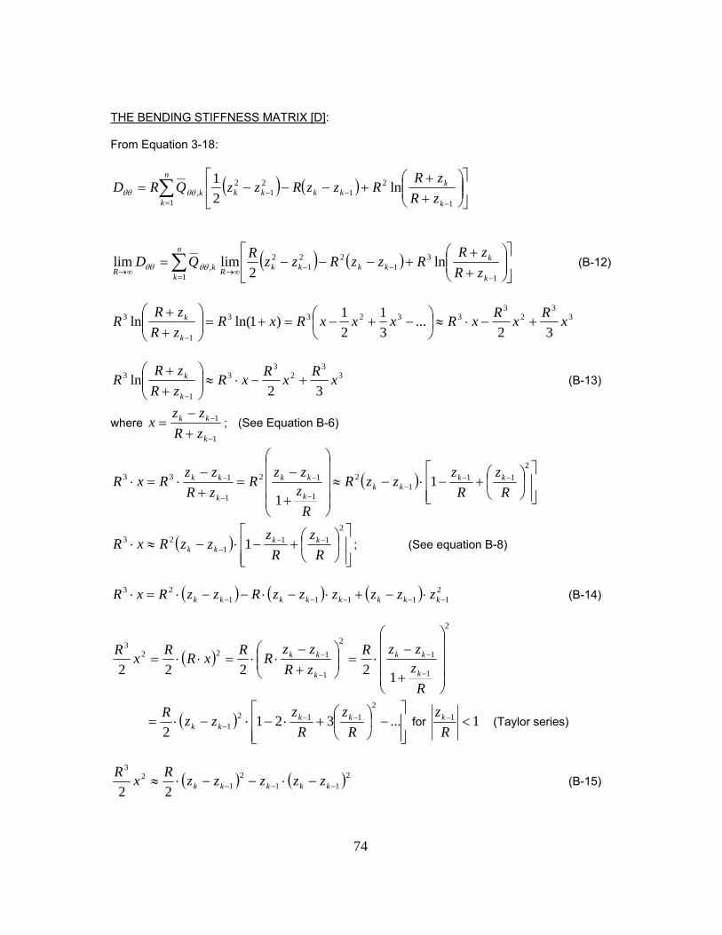
74

THE BENDING STIFFNESS MATRIX [D]: From Equation 3-18:

( ) ( )∑= −

−− ⎥⎦

⎤⎢⎣

⎡⎟⎟⎠

⎞⎜⎜⎝

⎛++

+−−−=n

k k

kkkkkk zR

zRRzzRzzQRD

1 1

21

21

2,

__ln

21

θθθθ

( ) ( )∑= −

−−∞→∞→⎥⎦

⎤⎢⎣

⎡⎟⎟⎠

⎞⎜⎜⎝

⎛++

+−−−=n

k k

kkkkkRkR zR

zRRzzRzzRQD

1 1

31

221

2,

__ln

2limlim θθθθ (B-12)

33

23

33233

1

3

32...

31

21)1ln(ln xRxRxRxxxRxR

zRzR

Rk

k +−⋅≈⎟⎠⎞

⎜⎝⎛ −+−=+=⎟⎟

⎠

⎞⎜⎜⎝

⎛++

−

33

23

3

1

3

32ln xRxRxR

zRzR

Rk

k +−⋅≈⎟⎟⎠

⎞⎜⎜⎝

⎛++

−

(B-13)

where 1

1

−

−

+−

=k

kk

zRzz

x ; (See Equation B-6)

( )⎥⎥⎦

⎤

⎢⎢⎣

⎡⎟⎠⎞

⎜⎝⎛+−⋅−≈

⎟⎟⎟⎟

⎠

⎞

⎜⎜⎜⎜

⎝

⎛

+

−=

+−

⋅=⋅ −−−

−

−

−

−2

111

2

1

12

1

133 11 R

zR

zzzR

Rzzz

RzRzz

RxR kkkk

k

kk

k

kk

( )⎥⎥⎦

⎤

⎢⎢⎣

⎡⎟⎠⎞

⎜⎝⎛+−⋅−≈⋅ −−

−

211

123 1

Rz

Rz

zzRxR kkkk ; (See equation B-8)

( ) ( ) ( ) 2

1111123

−−−−− ⋅−+⋅−⋅−−⋅=⋅ kkkkkkkk zzzzzzRzzRxR (B-14)

( )

2

1

1

2

1

1223

12222⎟⎟⎟⎟

⎠

⎞

⎜⎜⎜⎜

⎝

⎛

+

−⋅=⎟⎟

⎠

⎞⎜⎜⎝

⎛+−

⋅⋅=⋅⋅=−

−

−

−

RzzzR

zRzz

RRxRRxRk

kk

k

kk

( )⎥⎥⎦

⎤

⎢⎢⎣

⎡−⎟

⎠⎞

⎜⎝⎛+⋅−⋅−⋅= −−

− ...3212

2112

1 Rz

Rz

zzR kkkk for 11 <−

Rzk (Taylor series)

( ) ( )211

21

23

22 −−− −⋅−−⋅≈ kkkkk zzzzzRxR (B-15)

75

( ) ( )31

3

1

1333

31

31

31

3 −−

− −⋅≈⎟⎟⎠

⎞⎜⎜⎝

⎛+−

⋅⋅=⋅⋅= kkk

kk zzzRzz

RxRxR (B-16)

(Using the same approach in Equation B-15) Substitute B-14, B-15, and B-16 into B-12 yields:

( ) ( ) ( )

( ) ( ) ( )

( ) ( )

∑=

−∞→−−∞→

−∞→−−∞→−−∞→

−∞→−∞→−∞→

∞→

⎥⎥⎥⎥⎥⎥⎥

⎦

⎤

⎢⎢⎢⎢⎢⎢⎢

⎣

⎡

−⋅+−⋅+

−⋅−⋅−+⋅−⋅−

−⋅+−−−

=n

k

kkRkkkR

kkRkkkRkkkR

kkRkkRkkR

kR

zzzzz

zzRzzzzzzR

zzRzzRzzR

QD1

31

211

21

21111

12

122

12

,

__

31limlim

2limlimlim

limlim2

lim

lim θθθθ

( ) ( ) ( )

( )∑=

−−−−−∞→

−−−−−

∞→

⎥⎥⎥⎥

⎦

⎤

⎢⎢⎢⎢

⎣

⎡

−⋅+−⋅+⋅−−+

−⋅+−⋅+⋅−=

n

kkkkkkkkkkR

kkkkkkkk

kRzzzzzzzzzR

zzzzzzzzQD

1 211

2211

21

2

31

211

211

,

__

2222

lim

31

lim θθθθ

( ) ( ) ( )∑=

−−−−−∞→ ⎥⎦⎤

⎢⎣⎡ −⋅+−⋅+⋅−=

n

kkkkkkkkkkR

zzzzzzzzQD1

31

211

211,

__

31lim θθθθ

( )∑=

−∞→−=

n

kkkkR

zzQD1

31

3,

__

31lim θθθθ (Plate Lamination Theory).

76

REFERENCES

1) Sayegh A. F. and Dong S. B., M.ASCE, “Analysis of Laminated Curved Beams”,

Journal of the Engineering Mechanics Division, August 1970.

2) Cheung C. K. and Sorensen H. C., “Effect of axial loads on radial stress in curved

beams”, Wood and Fiber Science Journal, Volume 15, Number 3 / July 1983.

3) Graff E. and Springer G. S., “Stress analysis of thick, curved composite laminates”,

Computers & Structures journal, Volume 38, Issue 1, 1991, Pages 41-55.

4) Barbero, E. J., Fu, S. H., and Raftoyiannis, I., “Ultimate bending strength of composite

beams “, ASCE J. Mater, Civil Engng 3, 1991, pp. 293-306.

5) Madabhusi-Raman, P. and Davalos J. F., Static shear correction factor for laminated

rectangular beams. Composites Part B: Engineering, 1996. 27(3-4): p. 285-293.

6) Kasal B. and Heiduschle A., “Radial reinforcement of curved glue laminated wood

beams with composite materials”, Forest Products Journal, Jan 2004.

7) Wang W. and Shenoi R. A., “Analytical Solutions to Predict Flexural Behavior of Curved

Sandwich Beams”, Journal of Sandwich Structures and Materials, Vol. 6, No. 3, 199-

216 (2004).

8) Qatu M. S., Vibration of Laminated Shells and Plates, Elsevier Academic Press, 2004.

9) Ugural A. C. and Fenster S. K., Advanced Strength and Applied Elasticity 4th ed.,

Pearson Education, Inc., 2003.

10) Daniel, I.M. and Ishai, O., Engineering Mechanics of Composite Materials, 2nd edition,

Oxford University Press, 2006.

11) Chan W. S., Composite Lecture Notes, University of Texas at Arlington, Spring 2008.

77

BIOGRAPHICAL INFORMATION

Thien Nguyen received his Bachelor Degree in Mechanical Engineering from the

University of Texas at Arlington in 2007. He graduated with Summa Cum Laude Honor and

received numerous recognitions during his years as a undergraduate student. Thien was a

member of both Pi Tau Sigma and Alpha Chi Honor Society.

He started his Master’s degree in Mechanical Engineering at the University of Texas at

Arlington immediately after he received his Bachelor’s Degree. While pursuing his Master’s

Degree, Thien works for Vought Aircraft Industry as a Structural Engineer.

His research interests include composite structure analysis, finite element analysis, and

behavior of composite materials. Thien Nguyen received Master of Science Degree in

Mechanical Engineering from the University of Texas at Arlington in May 2010.

EFFECTS OF CURVATURE ON THE STRESSES by THIEN NGUYEN ...

Documents

Transcript of EFFECTS OF CURVATURE ON THE STRESSES by THIEN NGUYEN ...