EE123 Digital Signal Processing - EECS Instructional ...ee123/sp16/Notes/Lecture10_STFT... ·...

M. Lustig, EECS UC Berkeley

EE123Digital Signal Processing

Lecture 10Time-Dependent FT


Announcements!

• Midterm: 02/22/2016– Open everything–... but cheat sheet recommended instead– 10am-12pm

• How’s the lab going?

Frequency Analysis with DFT

Length of window determines spectral resolution

Type of window determines side-lobe amplitude.(Some windows have better tradeo↵ betweenresolution-sidelobe)

Zero-padding approximates the DTFT better. Does notintroduce new information!

Miki Lustig UCB. Based on Course Notes by J.M Kahn Spring 2014, EE123 Digital Signal Processing

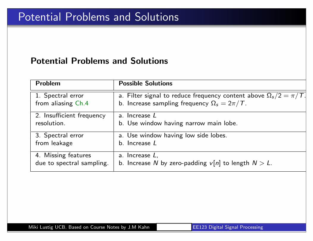
Potential Problems and Solutions

Potential Problems and Solutions

Problem Possible Solutions

1. Spectral error a. Filter signal to reduce frequency content above ⌦

s

/2 = ⇡/T .

from aliasing Ch.4 b. Increase sampling frequency ⌦

s

= 2⇡/T .

2. Insu�cient frequency a. Increase L

resolution. b. Use window having narrow main lobe.

3. Spectral error a. Use window having low side lobes.

from leakage b. Increase L

4. Missing features a. Increase L,

due to spectral sampling. b. Increase N by zero-padding v [n] to length N > L.

Miki Lustig UCB. Based on Course Notes by J.M Kahn Spring 2014, EE123 Digital Signal Processing

H(ej!)x[n] y[n]


Subtleties in filtering/processing with DFT

• System is implemented by overlap-and-save• Filtering using DFT

H[k]

π 2π0


Subtleties in filtering/processing with DFTH[k] h[n]

H(ejw)

π-π

π 2π0


Last Time

• Frequency Analysis with DFT• Windowing• Zero-Padding

• Today:– Time-Dependent Fourier Transform– Heisenberg Boxes


Discrete Transforms (Finite)

• DFT is only one out of a LARGE class of transforms

• Used for:–Analysis–Compression–Denoising–Detection–Recognition–Approximation (Sparse)

Sparse representation has been one of the hottest research topics in the last 15 years in sp

• Spectrum of a bird chirping– Interesting,.... but...– Does not tell the whole story– No temporal information!


Example: Bird Chirp

Play Sound!

0 0.5 1 1.5 2 2.5

x 104

0

100

200

300

400

500

600

Hz

Spectrum of a bird chirp

No temporal information!

Miki Lustig UCB. Based on Course Notes by J.M Kahn Fall 2011, EE123 Digital Signal Processing

Example of spectral analysis

x[n]

n

• To get temporal information, use part of the signal around every time point

• Mapping from 1D ⇒ 2D, n discrete, w cont.

• Simply slide a window and compute DTFTM. Lustig, EECS UC Berkeley

Time Dependent Fourier Transform

X[n,!) =1X

m=�1x[n+m]w[m]e�j!m

*Also called Short-time Fourier Transform (STFT)

• To get temporal information, use part of the signal around every time point


Time Dependent Fourier Transform

X[n,!) =1X

m=�1x[n+m]w[m]e�j!m

*Also called Short-time Fourier Transform (STFT)


Spectrogram

Time, s

Fre

quency, H

z

2 4 6 8 10 12 14 16 180

1000

2000

3000

4000

0 500 1000 1500 2000 2500 3000 3500 4000 45000

5

10

15

20

25

30

Frequency, Hz

0 500 1000 1500 2000 2500 3000 3500 4000 45000

2

4

6

8

10

12

Frequency, Hz

0 500 1000 1500 2000 2500 3000 3500 4000 45000

5

10

15

20

25

30

Frequency, Hz

0 500 1000 1500 2000 2500 3000 3500 4000 45000

2

4

6

8

10

12

Frequency, Hz

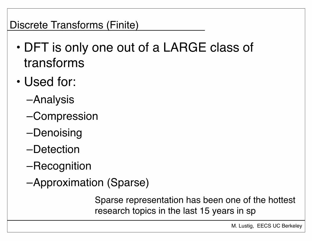
Xr[k] =L�1X

m=0

x[rR+m]w[m]e�j2⇡km/N


Discrete Time Dependent FT

• L - Window length• R - Jump of samples • N - DFT length

• Tradeoff between time and frequency resolution

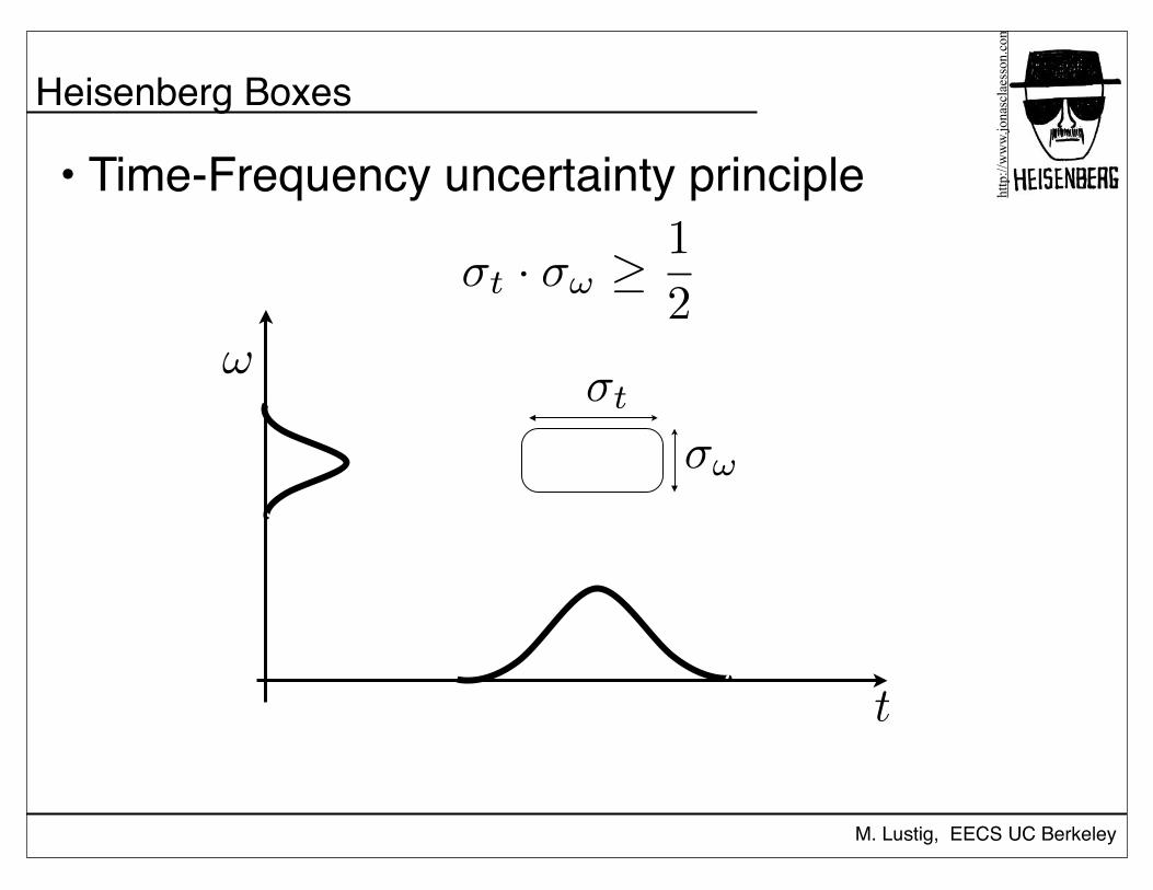
t

!

�t · �! � 1

2

�t

�!


Heisenberg Boxes

• Time-Frequency uncertainty principle http://www.jonasclaesson.com

�! =2⇡

N

�t = N

�! ·�t = 2⇡


DFT

X[k] =N�1X

n=0

x[n]e�j2⇡kn/N

!

tone DFT coefficient

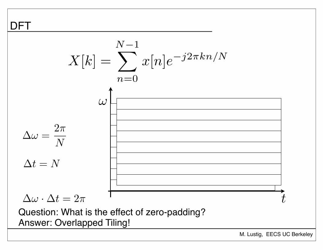
�! =2⇡

N

�t = N

�! ·�t = 2⇡


DFT

X[k] =N�1X

n=0

x[n]e�j2⇡kn/N

!

tQuestion: What is the effect of zero-padding?Answer: Overlapped Tiling!

X[r, k] =L�1X

m=0


�! =2⇡

L

�t = L


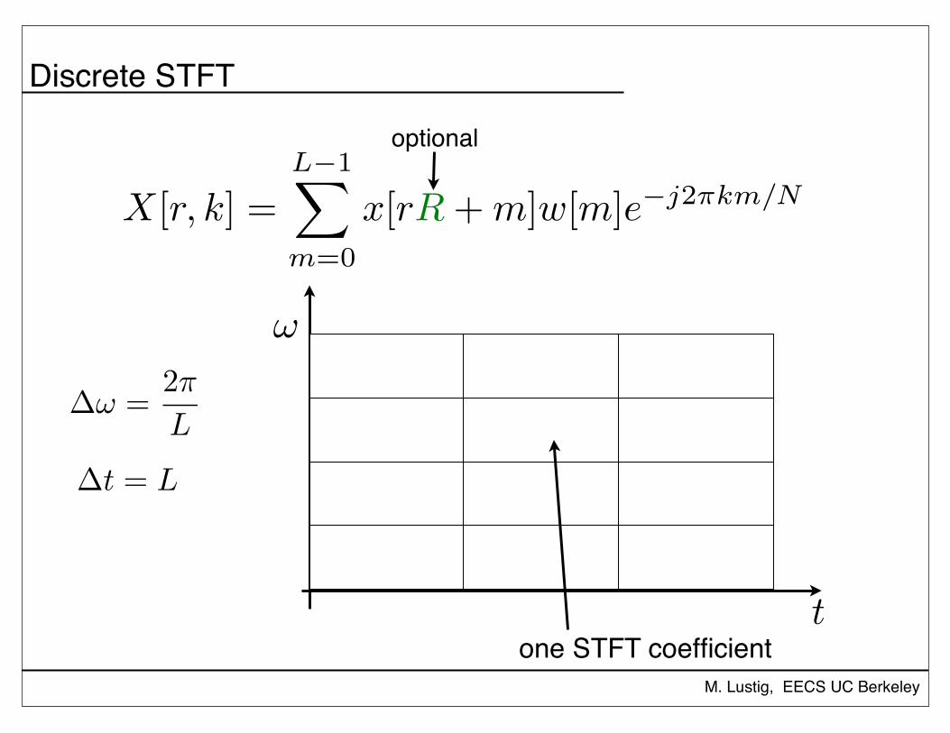
Discrete STFT

optional

!

tone STFT coefficient

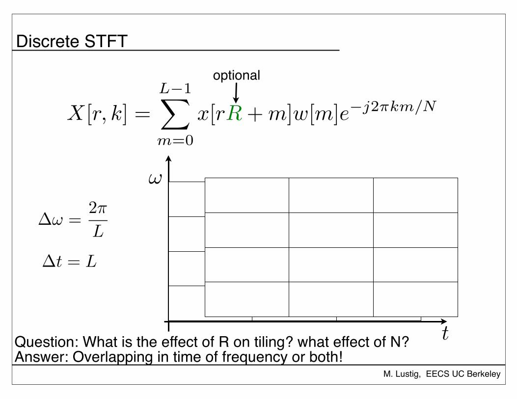
X[r, k] =L�1X

m=0


�! =2⇡

L

�t = L


Discrete STFT

optional

!

tQuestion: What is the effect of R on tiling? what effect of N?Answer: Overlapping in time of frequency or both!

Time, s

Fre

qu

en

cy,

Hz

1 2 3 4 5 6 7 80

1000

2000

3000

4000


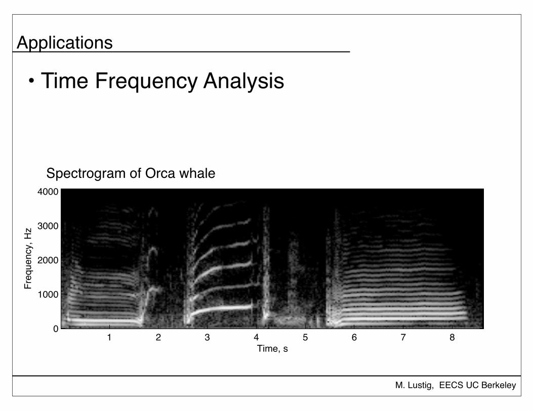
Applications

• Time Frequency Analysis

Spectrogram of Orca whale

Time, s

Freq

uenc

y, H

z

2 4 6 8 10 12 14 16 180

1000

2000

3000

4000


Spectrogram

• What is the difference between the spectrograms?

Time, s

Freq

uenc

y, H

z

2 4 6 8 10 12 14 16 180

1000

2000

3000

4000

a) Window size B<Ab) Window size B>A

(B)

(A)

c) Window type is differentd) (A) uses overlapping window


Windows Examples

Here we consider several examples. As before, the sampling rate is!s

/2⇡ = 1/T = 20 Hz.Rectangular Window, L = 32

0 5 10 15 20 25 300

0.2

0.4

0.6

0.8

1

1.2

n

w[n

]

Rectangular Window, L = 32

-20 -10 0 10 200

5

10

15

20

25

30

35

40

/2 (Hz)

|W(ejT)|

DTFT of Rectangular Window

0 5 10 15 20 25 30

-1.5

-1

-0.5

0

0.5

1

1.5

n

v[n]

Sampled, Windowed Signal, Rectangular Window, L = 32

-20 -10 0 10 200

5

10

15

20

/2 (Hz)

|V(ejT)|

DTFT of Sampled, Windowed Signal


Sidelobes of Hann vs rectangular windowWindows Examples

Hamming Window, L = 32

0 5 10 15 20 25 300

0.2

0.4

0.6

0.8

1

1.2

n

w[n

]


-20 -10 0 10 200

5

10

15

20

/2 (Hz)

|W(ejT)|

DTFT of Hamming Window

0 5 10 15 20 25 30

-1.5

-1

-0.5

0

0.5

1

1.5

n

v[n]

Sampled, Windowed Signal, Hamming Window, L = 32

-20 -10 0 10 200

2

4

6

8

10

/2 (Hz)

|V(ejT)|



Time, s

Freq

uenc

y, H

z

2 4 6 8 10 12 14 16 180

1000

2000

3000

4000


Spectrogram

• What is the difference between the spectrograms?

Time, s

Freq

uenc

y, H

z

2 4 6 8 10 12 14 16 180

1000

2000

3000

4000

a) Window size B<Ab) Window size B>A

c) Window type is differentd) (A) uses overlapping window

(A)

(B)


SpectrogramWindows Examples


0 5 10 15 20 25 300

0.2

0.4

0.6

0.8

1

1.2

n

w[n

]


-20 -10 0 10 200

5

10

15

20

/2 (Hz)

|W(ejT)|


0 5 10 15 20 25 30

-1.5

-1

-0.5

0

0.5

1

1.5

n

v[n]


-20 -10 0 10 200

2

4

6

8

10

/2 (Hz)

|V(ejT)|



Windows Examples


0 10 20 30 40 50 600

0.2

0.4

0.6

0.8

1

1.2

n

w[n

]


-20 -10 0 10 200

5

10

15

20

25

30

35

40

/2 (Hz)

|W(ejT)|


0 10 20 30 40 50 60

-1.5

-1

-0.5

0

0.5

1

1.5

n

v[n

]


-20 -10 0 10 200

5

10

15

20

/2 (Hz)

|V(ejT)|




Spectrogram of FM

n

Original Signal

Overlapping

Hann Windows

N Samples

M Samples

Figure 6: Extracting segments of a long signal with a Hann window

how the frequency resolution improves, while the temporal resolution degrades.

Task 5: Time-Frequency plots of the radio-frequency spectrum with the SDR.

The samples that are obtained by the SDR represent a bandwidth of the spectrum around a center fre-quency. Hence, when demodulating to base-band (i.e. zero frequency) the signal must be imaginary sinceit has a non symmetric Fourier transform. In this case, we would like to display both sides of the spectrum.

Modify the function myspectrogram(x,m,fs) such that it detects if the input signal x is complex. Inthat case, it will compute a double sided spectrum that is centered around DC. For this, it would we usefulto use the matlab commands: isreal and fftshift.

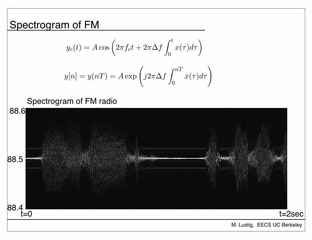
We will first look at radio FM spectrum. In the US the broadcast FM radio band is 88.1-107.9Mhz.It is split into 200KHz slots. This is relatively a large bandwidth and therefor it is also called widebandFM as opposed to narrowband FM which can be as low as 5 Khz. In FM radio the information is encodedby modulating the frequency of the carrier,

yc(t) = A cos✓2⇡fct+ 2⇡�f

Z t

0

x(⌧)d⌧◆.

Here, fc is the carrier frequency, �f is the frequency deviation and x(t) is a normalized baseband signal.

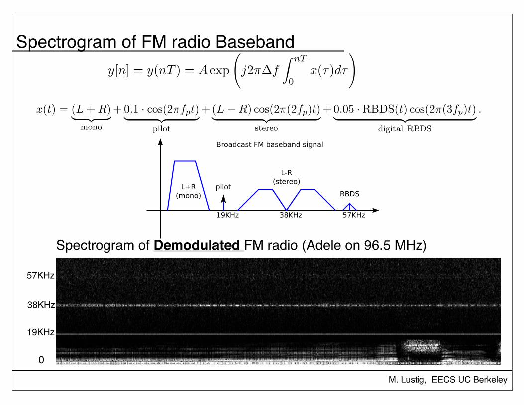
The broadcast FM baseband signal, x(t), consists of mono (Left+Right) Channels from 30Hz to 15 KHz,a pilot signal at fp = 19 KHz, amplitude modulated Stereo (Left - Right) channels around 2 · fp = 38KHzand digital RBDS, which encodes the station information, song name etc. at 3 · fp = 57KHz. (See

8

http://en.wikipedia.org/wiki/FM_broadcasting for more information). The baseband signal is:

x(t) = (L+R)| {z }

mono

+0.1 · cos(2⇡fpt)| {z }pilot

+(L�R) cos(2⇡(2fp)t)| {z }stereo

+0.05 · RBDS(t) cos(2⇡(3fp)t)| {z }digital RBDS

.

The signal RBDS(t) is a signal consists of ±1 at constant intervals which encode 0, and 1 bits. This is thespectrum of x(t):

Now, the SDR already demodulates by the carrier frequency fc, so the samples you get are actually

y[n] = y(nT ) = A exp

j2⇡�f

Z nT

0

x(⌧)d⌧

!

,

where T is the sampling rate.

Pick your favorite radio station (make sure there is good reception where you live! Don’t try it in thebasement or in rooms inside Cory that do not have windows). I’ve tested good reception from Cory hall5th floor at 88.5Mhz and 94.1Mhz. Acquire 4 seconds of data at a sampling rate of 200,000 Hz. Youcan use either rtl_tcp or rtl_sdr for that. Compute and display a spectrogram with a window of 500samples. Include the spectrogram in your report. What is the spectral and temporal resolution? Explainwhat you see. Don’t forget to play with di↵erent dynamic ranges of the spectrogram for best visualization.

In many analog radio systems, FM demodulation is performed by implementing a phased-locked loopthat tracks the frequency of the signal and extract the message x(t). However, it is very easy to implementan FM demodulation when the samples are discrete. Note, that the signal x(t) is proportional to theinstantaneous frequency of the signal. It is also proportional to the derivative of the phase! We can imple-ment this by computing the finite di↵erences of the phase of our signal angle(y[n])-angle(y[n-1]). Analternative that is robust to phase wrapping is to compute the product y[n]y⇤[n� 1] and then compute itsphase. Convince yourself that it works! In matlab it can be simply implemented by:

>> x = angle(y[2:end].*conj(y[1:end-1]));

FM demodulate the samples you got from the SDR and display the spectrogram. Note, that afterFMdemodulating the signal should be real and hence only half the spectrum should be displayed. Identify themono audio, the pilot, the stereo and the RBDS signals. Note, that the RBDS signal may be too weak todetect or may need better spectral resolution.

9

Spectrogram of FM radio

t=0 t=2sec

88.5

88.6

88.4


Spectrogram of FM radio Baseband


x(t) = (L+R)| {z }

mono




.




j2⇡�f

Z nT

0

x(⌧)d⌧

!

,






9


x(t) = (L+R)| {z }

mono




.


��

��

��

��

�� !" #��#�� $��



j2⇡�f

Z nT

0

x(⌧)d⌧

!

,






9


x(t) = (L+R)| {z }

mono




.




j2⇡�f

Z nT

0

x(⌧)d⌧

!

,






9

Spectrogram of Demodulated FM radio (Adele on 96.5 MHz)

0

19KHz

38KHz

57KHz


Subcarrier FM radio (Hidden Radio Stations)


Applications

• Time Frequency Analysis

Spectrogram of digital communications - Frequency Shift Keying

t=0 t=1sec

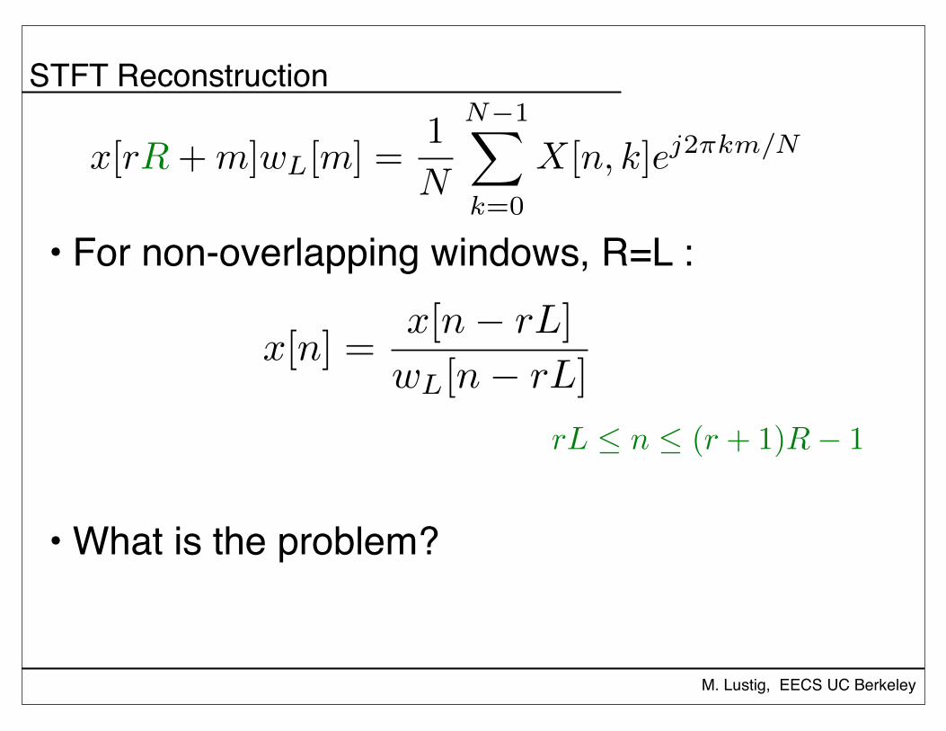
x[rR+m]wL[m] =1

N

N�1X

k=0

X[n, k]ej2⇡km/N


STFT Reconstruction

• For non-overlapping windows, R=L :

• What is the problem?

x[n] =x[n� rL]

wL[n� rL]

rL n (r + 1)R� 1

x[rR+m]wL[m] =1

N

N�1X

k=0

X[n, k]ej2⇡km/N


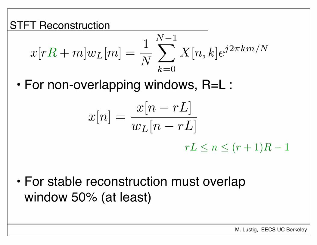
STFT Reconstruction

• For non-overlapping windows, R=L :

• For stable reconstruction must overlap window 50% (at least)

x[n] =x[n� rL]

wL[n� rL]

rL n (r + 1)R� 1


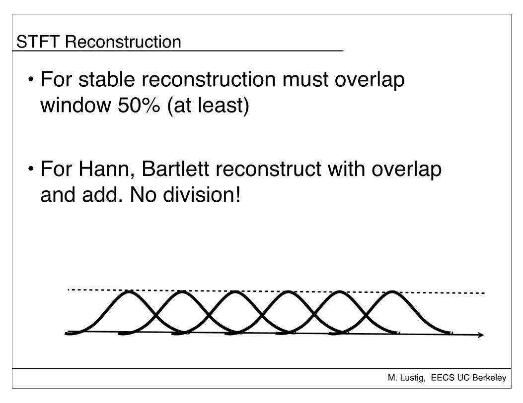
STFT Reconstruction

• For stable reconstruction must overlap window 50% (at least)

• For Hann, Bartlett reconstruct with overlap and add. No division!


Applications

• Noise removal

• Recall bird chirp x[n]

n

Example: Bird Chirp

Play Sound!

0 0.5 1 1.5 2 2.5

x 104

0

100

200

300

400

500

600

Hz

Spectrum of a bird chirp

No temporal information!



Application

• Denoising of Sparse spectrograms

• Spectrum is sparse! can implement adaptive filter, or just threshold!

Time, s

Fre

quency, H

z

2 4 6 8 10 12 14 16 180

1000

2000

3000

4000


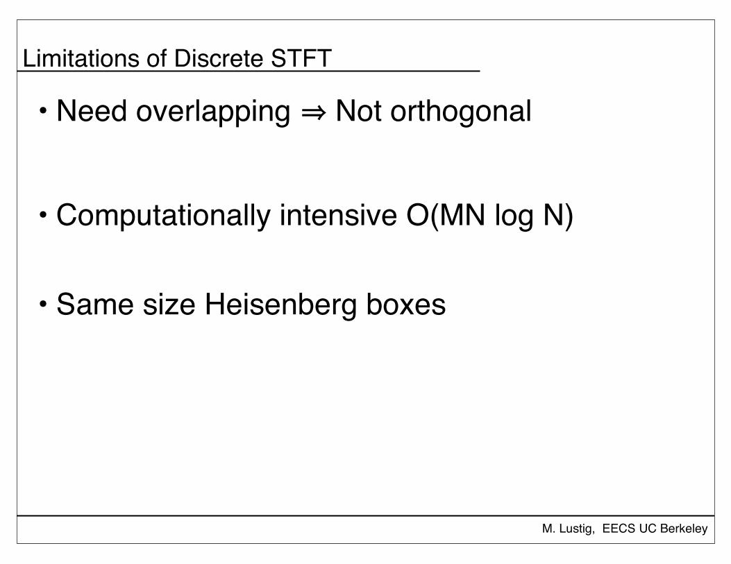
Limitations of Discrete STFT

• Need overlapping ⇒ Not orthogonal

• Computationally intensive O(MN log N)

• Same size Heisenberg boxes


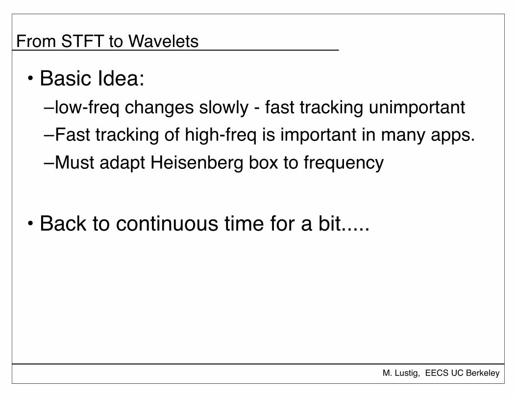
From STFT to Wavelets

• Basic Idea:–low-freq changes slowly - fast tracking unimportant–Fast tracking of high-freq is important in many apps.–Must adapt Heisenberg box to frequency

• Back to continuous time for a bit.....

EE123 Digital Signal Processing - EECS Instructional ...ee123/sp16/Notes/Lecture10_STFT... ·...

Documents

Transcript of EE123 Digital Signal Processing - EECS Instructional ...ee123/sp16/Notes/Lecture10_STFT... ·...