Review: DTFT

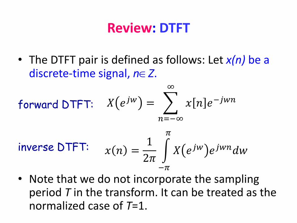
• The DTFT pair is defined as follows: Let x(n) be a discrete-time signal, nZ.

forward DTFT: inverse DTFT:

• Note that we do not incorporate the sampling period T in the transform. It can be treated as the normalized case of T=1.

𝑋 𝑒𝑗𝑤 = 𝑥 𝑛 𝑒−𝑗𝑤𝑛∞

𝑛=−∞

𝑥 𝑛 =1

2𝜋 𝑋 𝑒𝑗𝑤 𝑒𝑗𝑤𝑛𝑑𝑤

𝜋

−𝜋

Review: DTFT

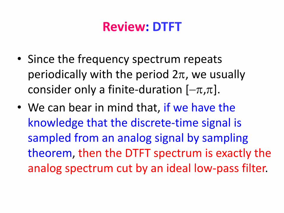
• Since the frequency spectrum repeats periodically with the period 2, we usually consider only a finite-duration [,].

• We can bear in mind that, if we have the knowledge that the discrete-time signal is sampled from an analog signal by sampling theorem, then the DTFT spectrum is exactly the analog spectrum cut by an ideal low-pass filter.

Review: DTFT

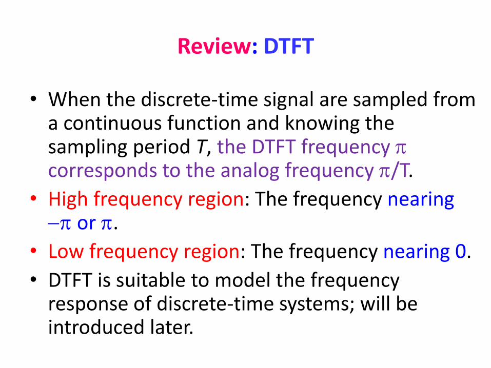
• When the discrete-time signal are sampled from a continuous function and knowing the sampling period T, the DTFT frequency corresponds to the analog frequency /T.

• High frequency region: The frequency nearing or .

• Low frequency region: The frequency nearing 0.

• DTFT is suitable to model the frequency response of discrete-time systems; will be introduced later.

This Week

• Discrete Fourier Transform (in short, DFT)

• Remember we have introduced three kinds of Fourier transforms.

• However, what we are able to deal with in the discrete-time domain is usually a finite-duration signal.

• DFT is the final (fourth) Fourier transform, where its input is a discrete-time finite-duration signal.

How to manipulate Frequencies in Discrete-time Domain?

Two Main Approaches

Details will be introduced in later courses

• Difference Equations

x[n]: input, y[n]: output

• That is, building a system that makes use of the current and previous inputs x[n], x[n-1], x[n-2] ….

as well as the previous outputs y[n-1], y[n-2], …

Linear System

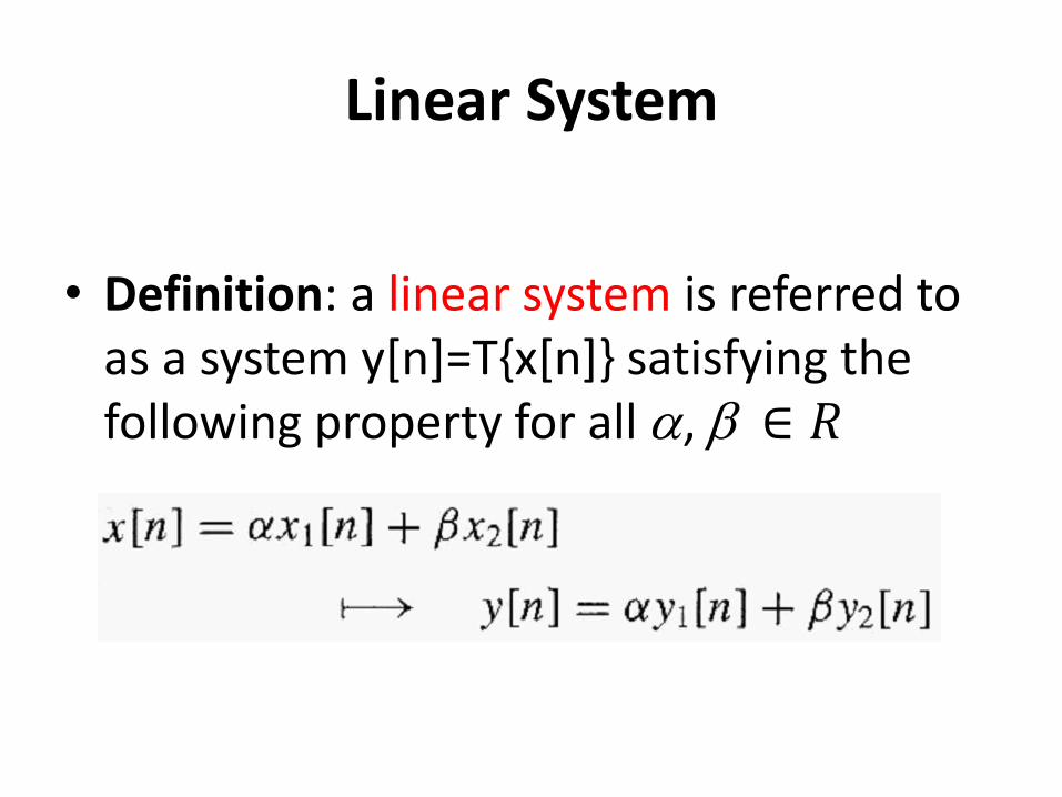
• Definition: a linear system is referred to as a system y[n]=T{x[n]} satisfying the following property for all , ∈ 𝑅

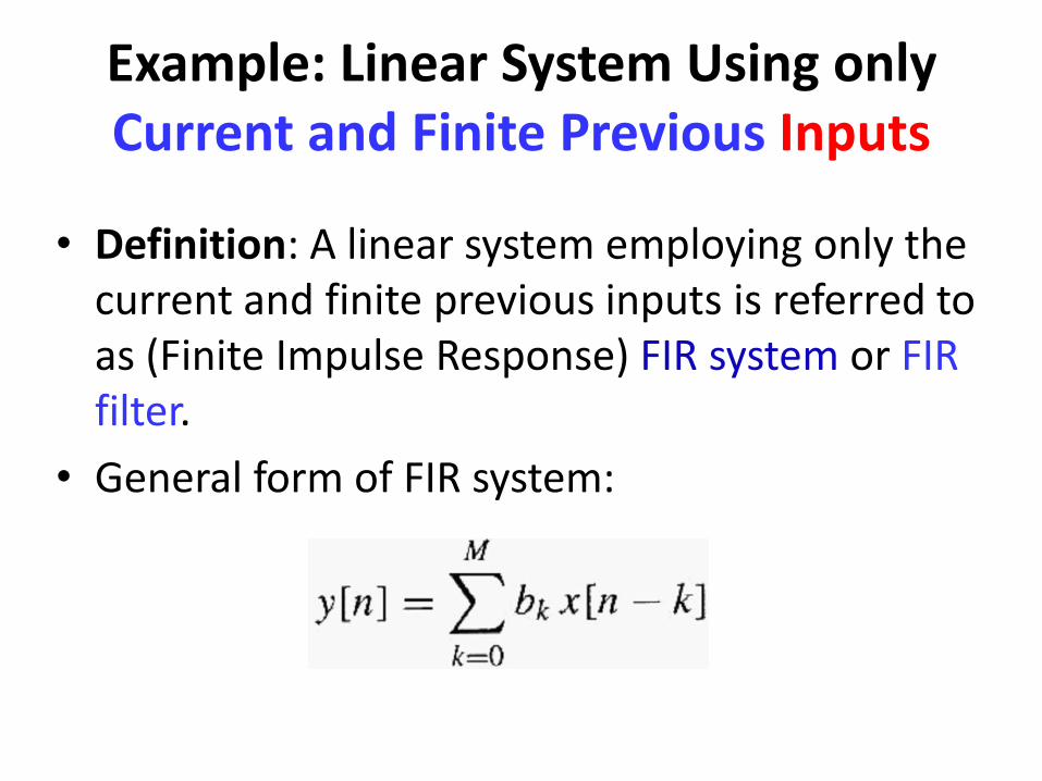
Example: Linear System Using only Current and Finite Previous Inputs

• Definition: A linear system employing only the current and finite previous inputs is referred to as (Finite Impulse Response) FIR system or FIR filter.

• General form of FIR system:

Example of FIR: running average filters

• 3-point running average filter:

• 7-point running average filter

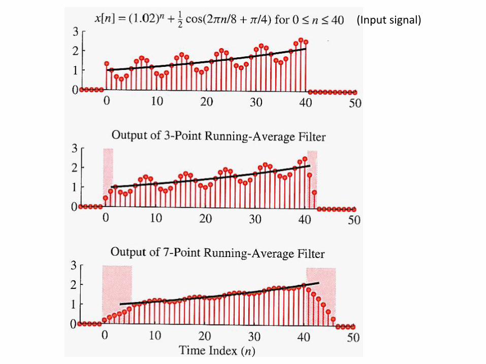
(Input signal)

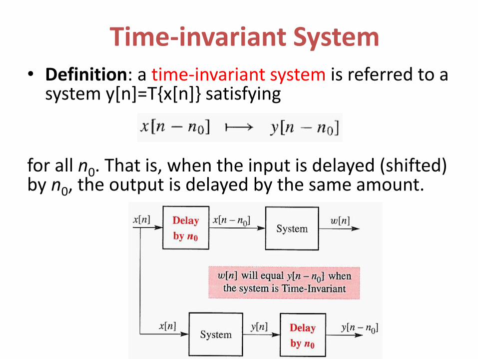
Time-invariant System • Definition: a time-invariant system is referred to a

system y[n]=T{x[n]} satisfying

for all n0. That is, when the input is delayed (shifted) by n0, the output is delayed by the same amount.

Linear Time-invariant (LTI) System

• It can be easily verified that the FIR filter of the form

is a time-invariant system.

Linear Time-invariant (LTI) System

• Definition: A system that is both linear and time-invariant is referred to as an LTI system.

• Example: FIR filter is an LTI system.

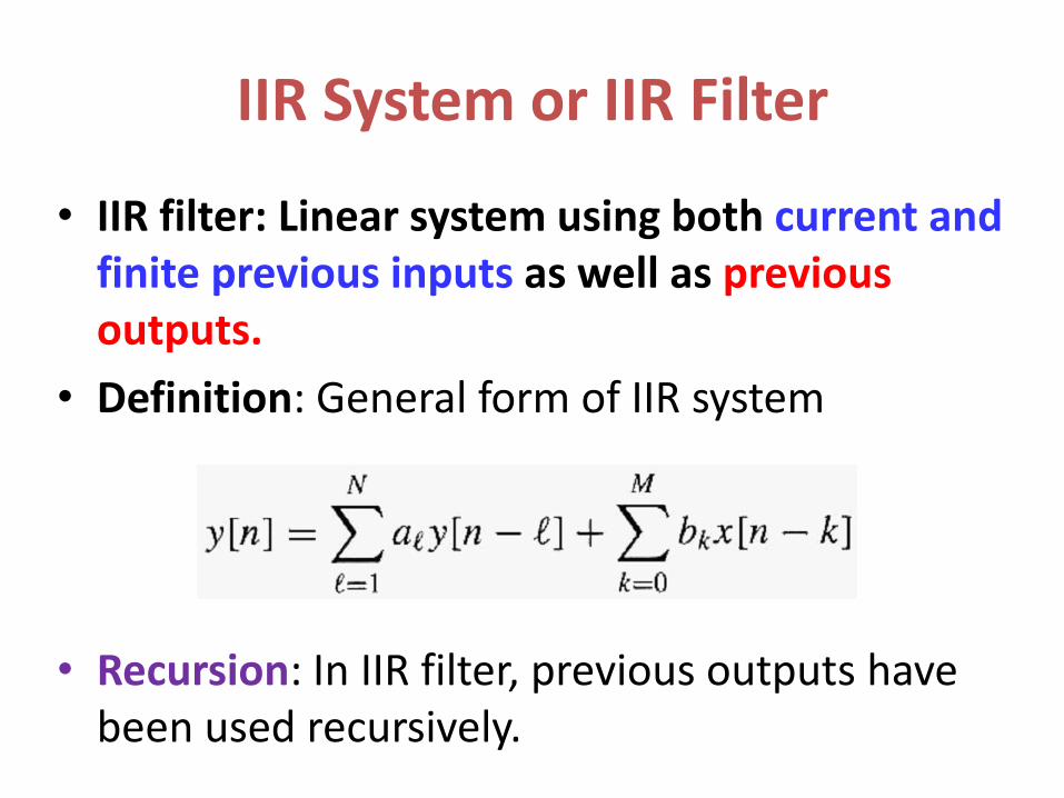
IIR System or IIR Filter

• IIR filter: Linear system using both current and finite previous inputs as well as previous outputs.

• Definition: General form of IIR system

• Recursion: In IIR filter, previous outputs have been used recursively.

General form of LTI system

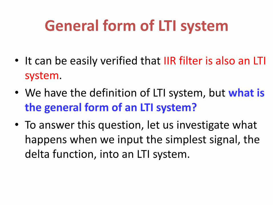
• It can be easily verified that IIR filter is also an LTI system.

• We have the definition of LTI system, but what is the general form of an LTI system?

• To answer this question, let us investigate what happens when we input the simplest signal, the delta function, into an LTI system.

General form of LTI system

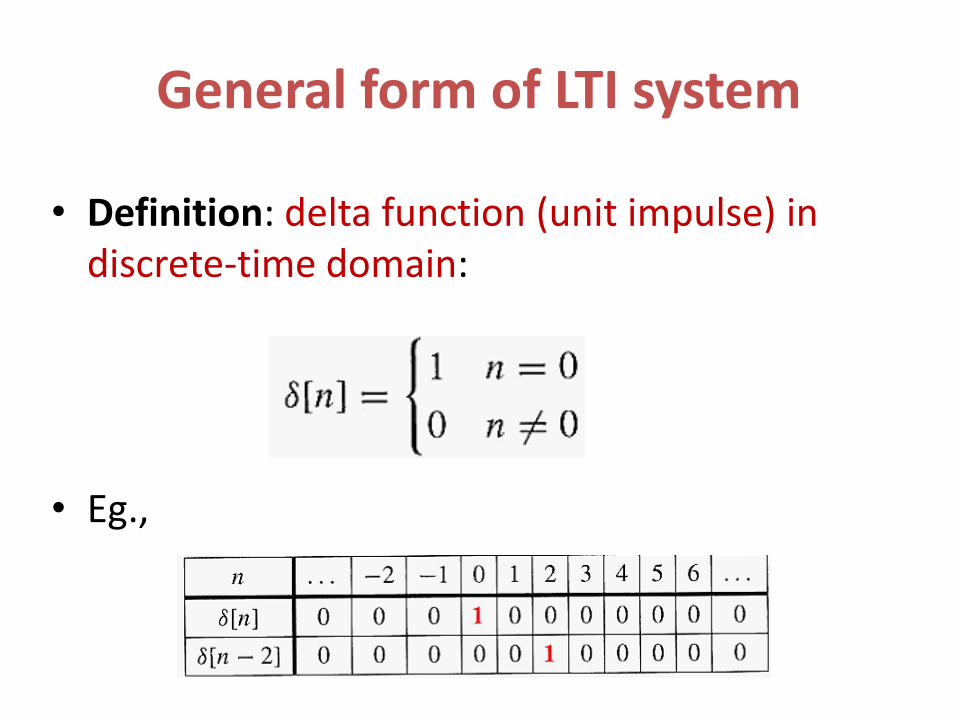
• Definition: delta function (unit impulse) in discrete-time domain:

• Eg.,

Impulse Response

• When taking the unit impulse [n] as input to a system, the output h[n] is called the impulse response of this system.

• Property: Any discrete-time signal x[n] can be represented as the linear combination of delayed unit-impulse functions, as shown below:

k

knkxnx

Impulse Response

• Then, we have the following property for the impulse response of an LTI system:

• So

[ ]

k

y n x k h n k

k

k

knTkx

knkxTny

by Time-invariance

by Linearity

Impulse Response

• Hence, when we know the impulse response h[n] of a linear system, then the output signal can be completely determined by the input signal and the impulse response from the above equation.

[ ]

k

y n x k h n k

Knowing an LTI system

Knowing its impulse response

equivalent to

Impulse Response

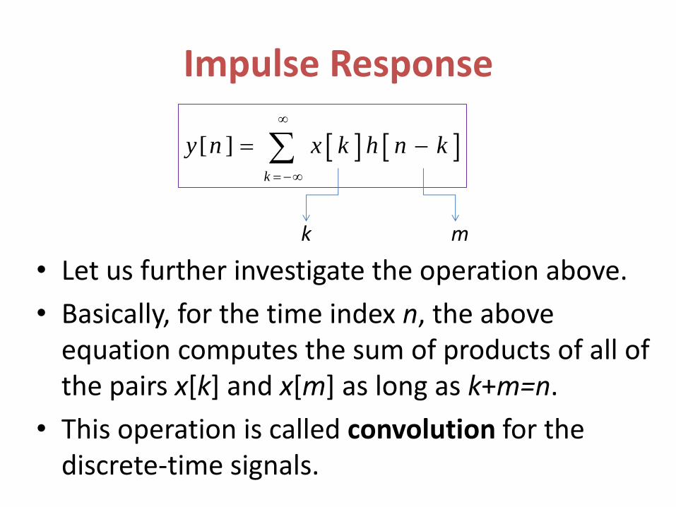
• Let us further investigate the operation above.

• Basically, for the time index n, the above equation computes the sum of products of all of the pairs x[k] and x[m] as long as k+m=n.

• This operation is called convolution for the discrete-time signals.

[ ]

k

y n x k h n k

k m

Convolution (for discrete-time signals)

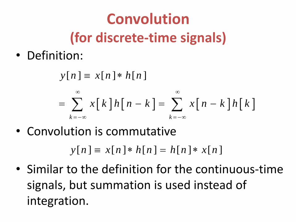
• Definition:

• Convolution is commutative

• Similar to the definition for the continuous-time signals, but summation is used instead of integration.

[ ] [ ] [ ]

k k

y n x n h n

x k h n k x n k h k

[ ] [ ] [ ] [ ] [ ]y n x n h n h n x n

Example

Example

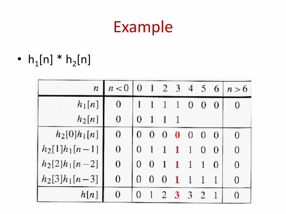
• h1[n] * h2[n]

Analogous to the arithmetic multiplication

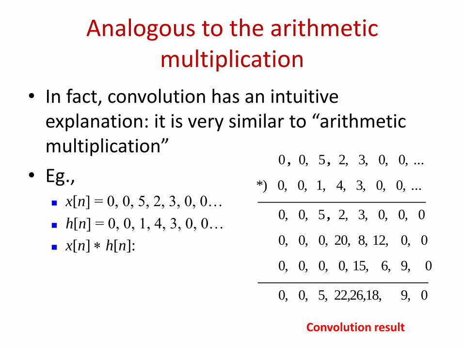
• In fact, convolution has an intuitive explanation: it is very similar to “arithmetic multiplication”

• Eg., x[n] = 0, 0, 5, 2, 3, 0, 0…

h[n] = 0, 0, 1, 4, 3, 0, 0…

x[n] h[n]:

0 9, 22,26,18, 5, 0, 0,

0 9, 6, 15, 0, 0, 0, 0,

0 0, 12, 8, 20, 0, 0, 0,

0 0, 0, 3, 2, 5 0, 0,

... 0, 0, 3, 4, 1, 0, 0, *)

... 0, 0, 3, 2, 5 0, 0

,

,,

Convolution result

Interpreted as Polynomial Multiplication

• Convolution can also be explained intuitively by polynomial multiplication:

• Consider f[n] h[n]

Response of LTI System

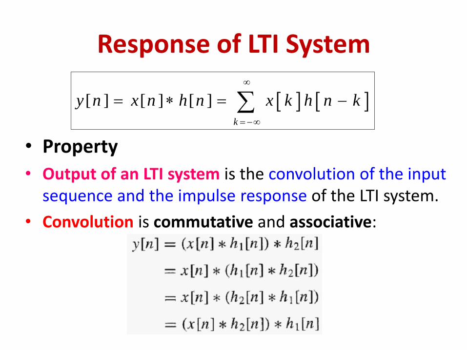
• Property

• Output of an LTI system is the convolution of the input sequence and the impulse response of the LTI system.

• Convolution is commutative and associative:

[ ] [ ] [ ]

k

y n x n h n x k h n k

Equivalent Systems

• Hence, we have the following equivalent systems:

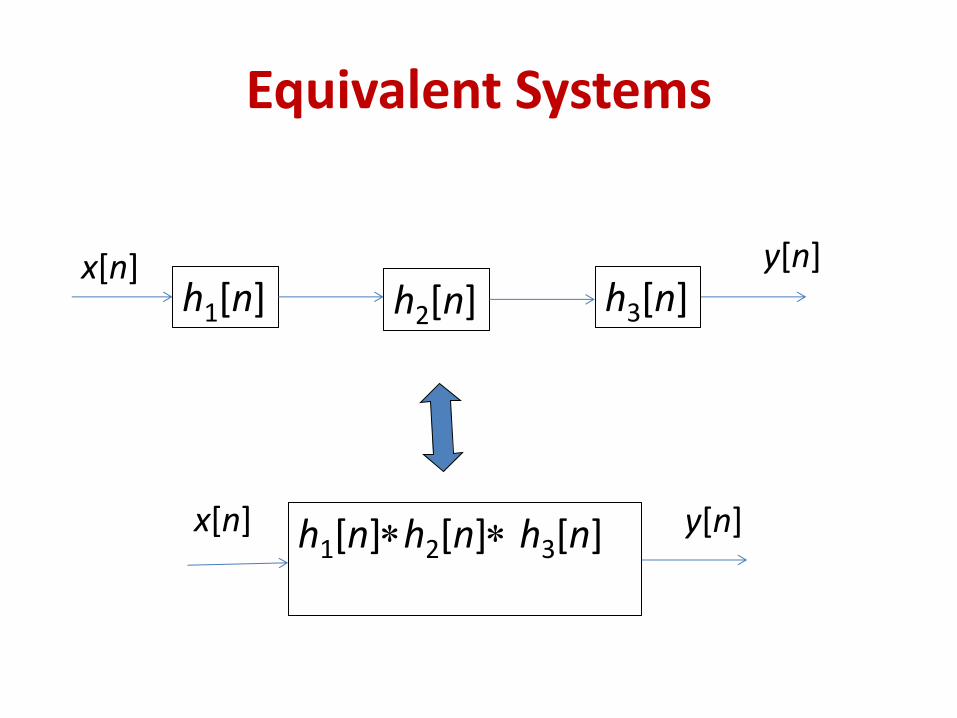
Equivalent Systems

h1[n] h2[n] h3[n]

x[n] y[n]

h1[n]h2[n] h3[n]

x[n] y[n]

Convolution and Equivalent System

• Property

• Convolution is also distributive over addition:

x[n] (h1[n] + h2[n]) = x[n] h1[n] + x[n] h2[n].

Ideal delay: h[n] = [n-nd]

Moving average

Accumulator

Forward difference: h[n] = [n+1][n]

Backward difference: h[n] = [n][n1]

Impulse Responses of Some LTI Systems

otherwise0

1

121

21

MnMMMnh

otherwise0

01 nnh

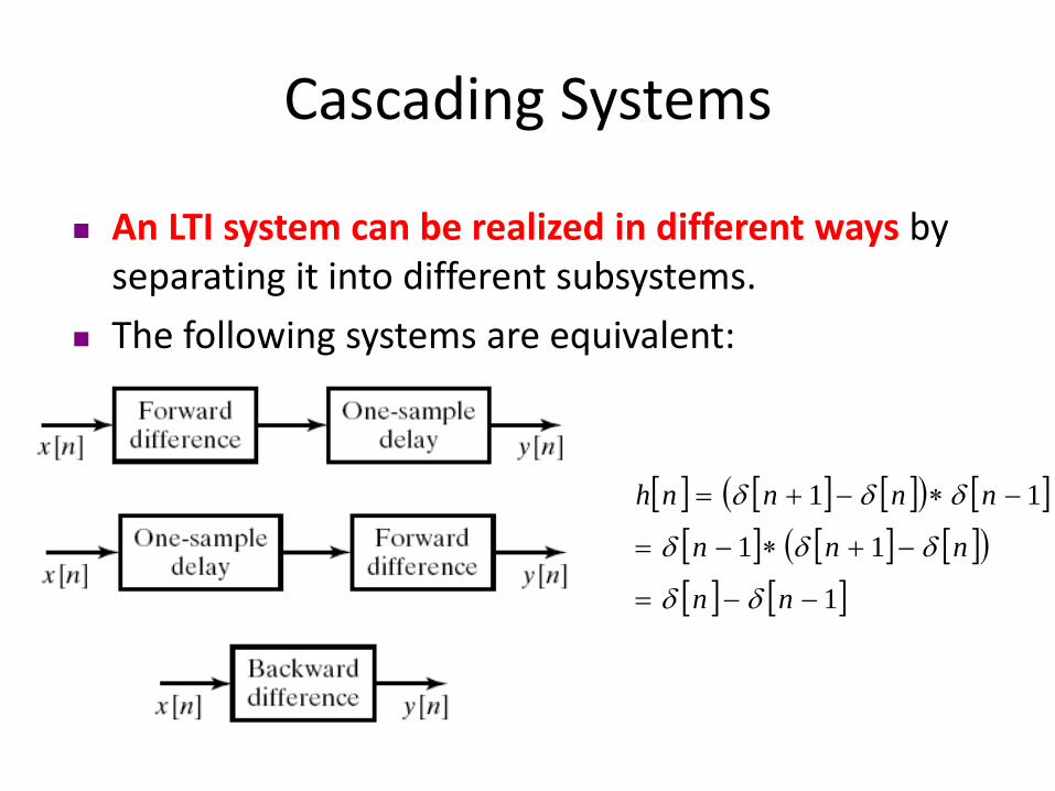
An LTI system can be realized in different ways by separating it into different subsystems.

The following systems are equivalent:

Cascading Systems

1

11

11

nn

nnn

nnnnh

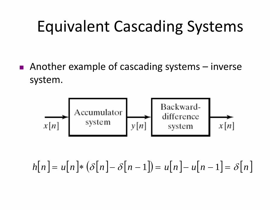
Another example of cascading systems – inverse system.

Equivalent Cascading Systems

nnununnnunh 11

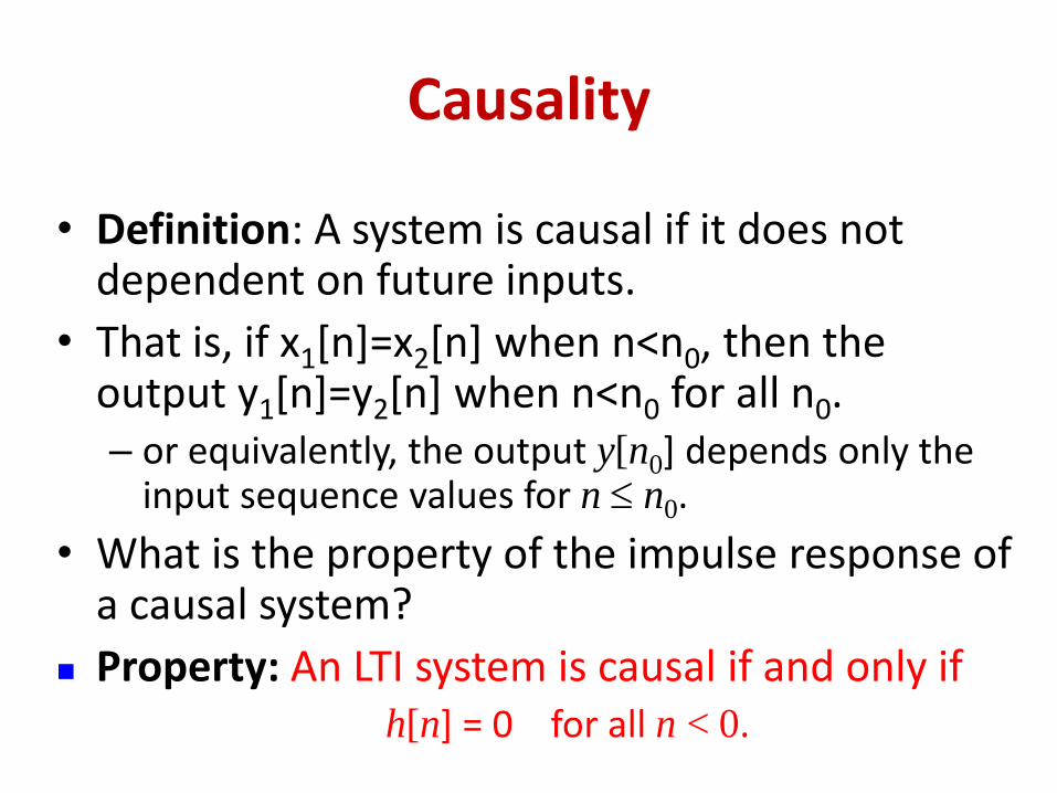
Causality

• Definition: A system is causal if it does not dependent on future inputs.

• That is, if x1[n]=x2[n] when n<n0, then the output y1[n]=y2[n] when n<n0 for all n0. – or equivalently, the output y[n0] depends only the

input sequence values for n n0.

• What is the property of the impulse response of a causal system?

Property: An LTI system is causal if and only if h[n] = 0 for all n < 0.

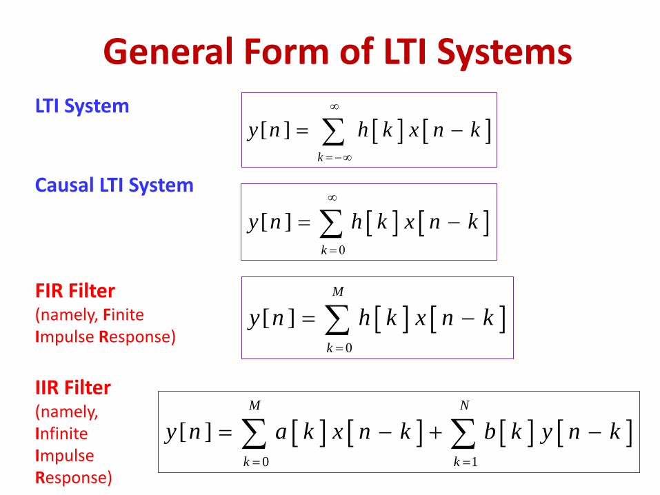
General Form of LTI Systems

LTI System

Causal LTI System

FIR Filter (namely, Finite Impulse Response)

IIR Filter (namely, Infinite Impulse Response)

[ ]

k

y n h k x n k

0

[ ]

k

y n h k x n k

0

[ ]

M

k

y n h k x n k

0 1

[ ]

M N

k k

y n a k x n k b k y n k

Difference Equation

• From the above, we can find that both FIR and IIR filters are causal LTI Systems.

• They are both difference equations. • Difference equation: (variables are functions. y: unknown function; x: given)

• Both FIR and IIR filters are solutions of difference equations.

• IIR filter is the case when a0=1. Difference equation is merely a more general form.

M

m

m

N

k

k mnxbknya

00

Realization of an LTI System

• Difference equation is an LTI system.

• Another important property is that difference equation is realizable by recursion:

– To realize or implement an LTI system, we cannot but exploit previously appeared (available) inputs and/or outputs.

• Question: Are all the LTI systems able to be implemented by using difference equations?

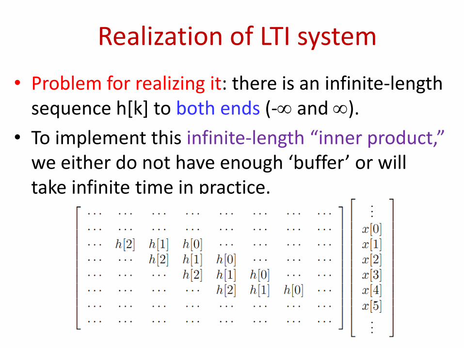
Illustration: (infinite-long) Matrix Vector

• A General LTI system is of the form:

• Can be explained as a infinite-dimensional matrix/vector product

[ ]

k

y n h k x n k

[ 3] [0] [ 1] [ 2 ] [ 3] [ 4 ] [ 5]

[ 2 ] [1] [0] [ 1] [ 2 ] [ 3] [ 4 ]

[ 1] [2 ] [1] [0] [ 1] [ 2 ] [ 3]

[0] [3] [2 ] [1] [0] [ 1] [ 2 ]

[1] [4 ] [3] [2 ] [1] [0

[2 ]

y h h h h h h

y h h h h h h

y h h h h h h

y h h h h h h

y h h h h h

y

[ 3]

[ 2 ]

[ 1]

[0]

] [ 1] [1]

[5] [4 ] [3] [2 ] [1] [0] [2 ]

x

x

x

x

h x

h h h h h h x

Realization of LTI system

• Problem for realizing it: there is an infinite-length sequence h[k] to both ends (- and ).

• To implement this infinite-length “inner product,” we either do not have enough ‘buffer’ or will take infinite time in practice.

Realization of LTI System

• By recursion, IIR filter can track back and approaches to one-side-infinity.

• We could allow the system to take future inputs (eg. future L samples), and delay the output by the same time-length L. With this idea, “IIR filter” becomes

• However, the range L is still finite. • We cannot implement the situation when L

approaches to infinity by difference equation. • In sum, we cannot realize the LTI system when the

impulse response has double-sided infinite-durations.

1

[ ]

M N

k L k L

y n L a k x n k b k y n k

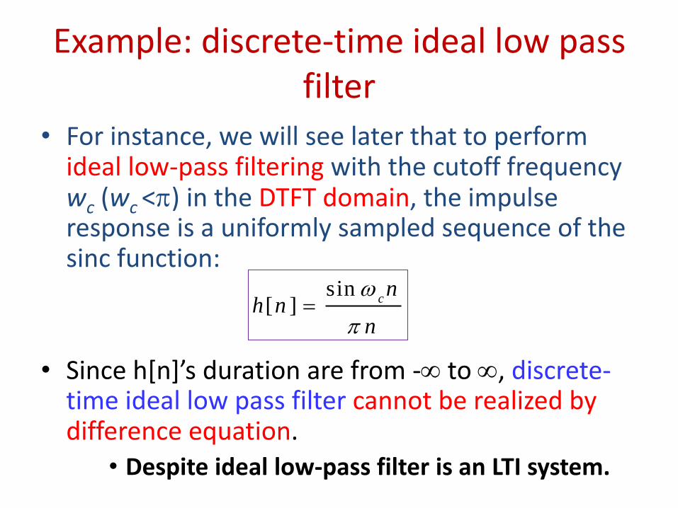
Example: discrete-time ideal low pass filter

• For instance, we will see later that to perform ideal low-pass filtering with the cutoff frequency wc (wc <) in the DTFT domain, the impulse response is a uniformly sampled sequence of the sinc function:

• Since h[n]’s duration are from - to , discrete-time ideal low pass filter cannot be realized by difference equation.

• Despite ideal low-pass filter is an LTI system.

sin[ ] c

nh n

n

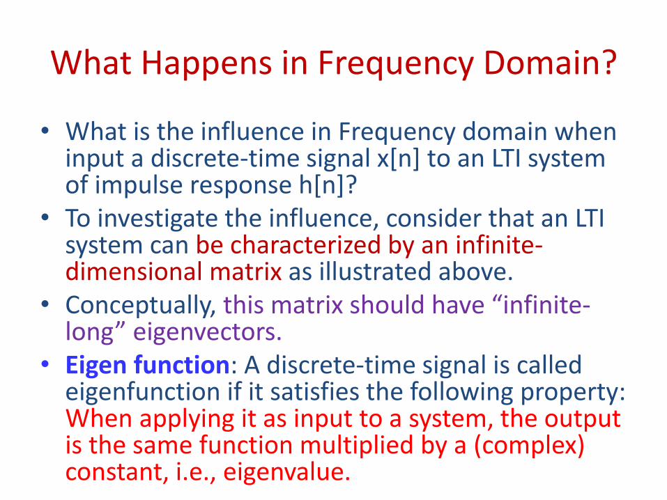
What Happens in Frequency Domain?

• What is the influence in Frequency domain when input a discrete-time signal x[n] to an LTI system of impulse response h[n]?

• To investigate the influence, consider that an LTI system can be characterized by an infinite-dimensional matrix as illustrated above.

• Conceptually, this matrix should have “infinite-long” eigenvectors.

• Eigen function: A discrete-time signal is called eigenfunction if it satisfies the following property: When applying it as input to a system, the output is the same function multiplied by a (complex) constant, i.e., eigenvalue.

Eigenfunction of LTI System

Property: x[n] = ejwn is the eigenfunction of all LTI systems (wR)

Pf: Let h[n] be the impulse response of an LTI system, when ejwn is applied as the input,

Let

we can see

k

jwkjwn

k

knjwekheekhny

k

jwkjwekheH

jwnjweeHny

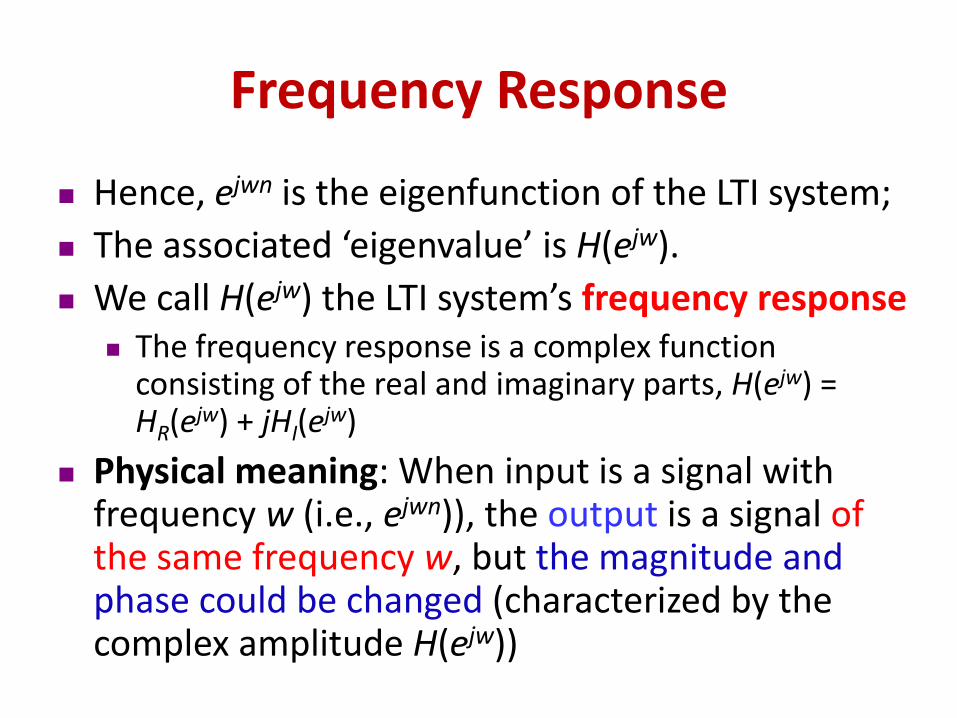
Frequency Response

Hence, ejwn is the eigenfunction of the LTI system;

The associated ‘eigenvalue’ is H(ejw).

We call H(ejw) the LTI system’s frequency response The frequency response is a complex function

consisting of the real and imaginary parts, H(ejw) = HR(ejw) + jHI(e

jw)

Physical meaning: When input is a signal with frequency w (i.e., ejwn)), the output is a signal of the same frequency w, but the magnitude and phase could be changed (characterized by the complex amplitude H(ejw))

Frequency Response

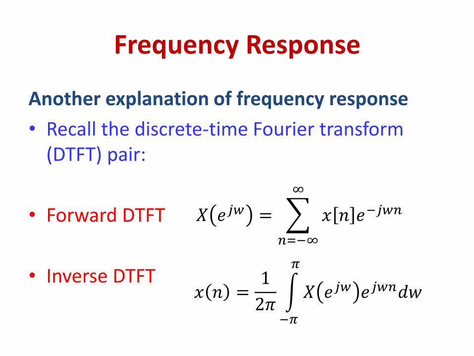
Another explanation of frequency response

• Recall the discrete-time Fourier transform (DTFT) pair:

• Forward DTFT

• Inverse DTFT

𝑋 𝑒𝑗𝑤 = 𝑥 𝑛 𝑒−𝑗𝑤𝑛∞

𝑛=−∞

𝑥 𝑛 =1

2𝜋 𝑋 𝑒𝑗𝑤 𝑒𝑗𝑤𝑛𝑑𝑤

𝜋

−𝜋

Frequency Response

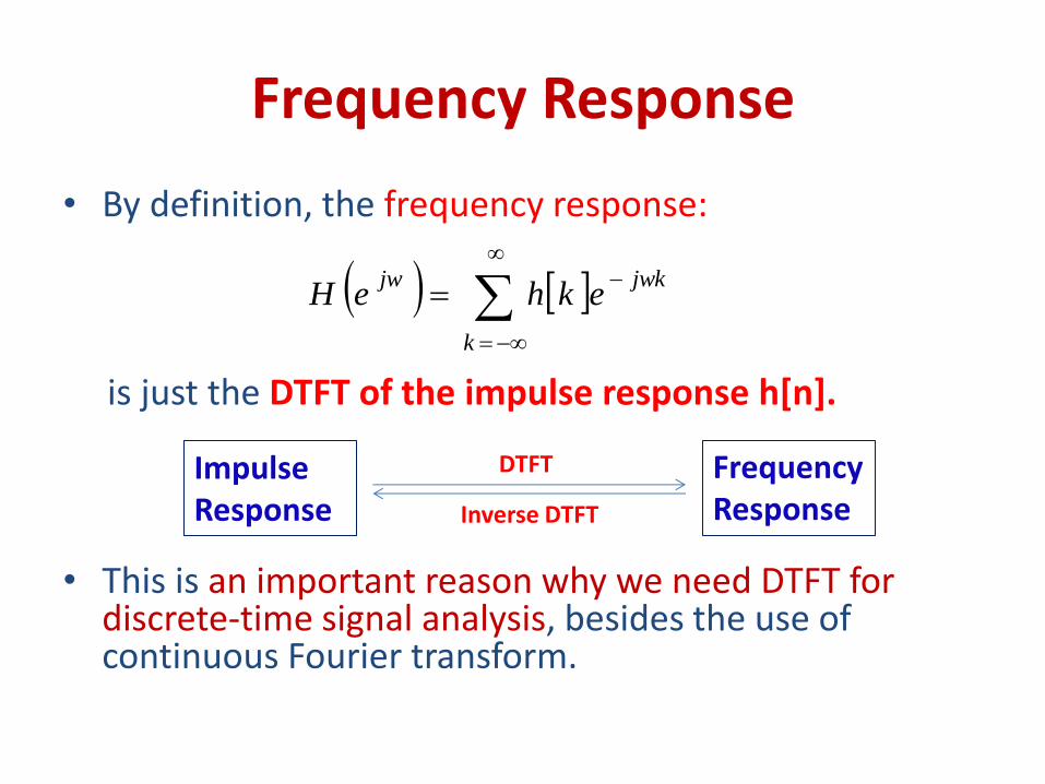
• By definition, the frequency response:

is just the DTFT of the impulse response h[n].

• This is an important reason why we need DTFT for discrete-time signal analysis, besides the use of continuous Fourier transform.

k

jwkjwekheH

Impulse Response

Frequency Response

DTFT

Inverse DTFT

LTI System and Frequency Response

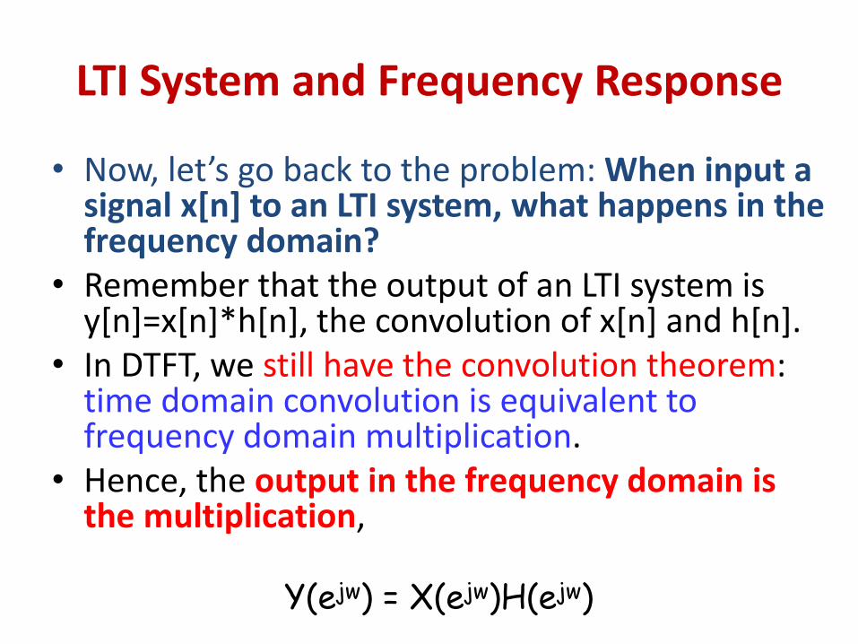
• Now, let’s go back to the problem: When input a signal x[n] to an LTI system, what happens in the frequency domain?

• Remember that the output of an LTI system is y[n]=x[n]*h[n], the convolution of x[n] and h[n].

• In DTFT, we still have the convolution theorem: time domain convolution is equivalent to frequency domain multiplication.

• Hence, the output in the frequency domain is the multiplication,

Y(ejw) = X(ejw)H(ejw)

Multiplication in Frequency Domain

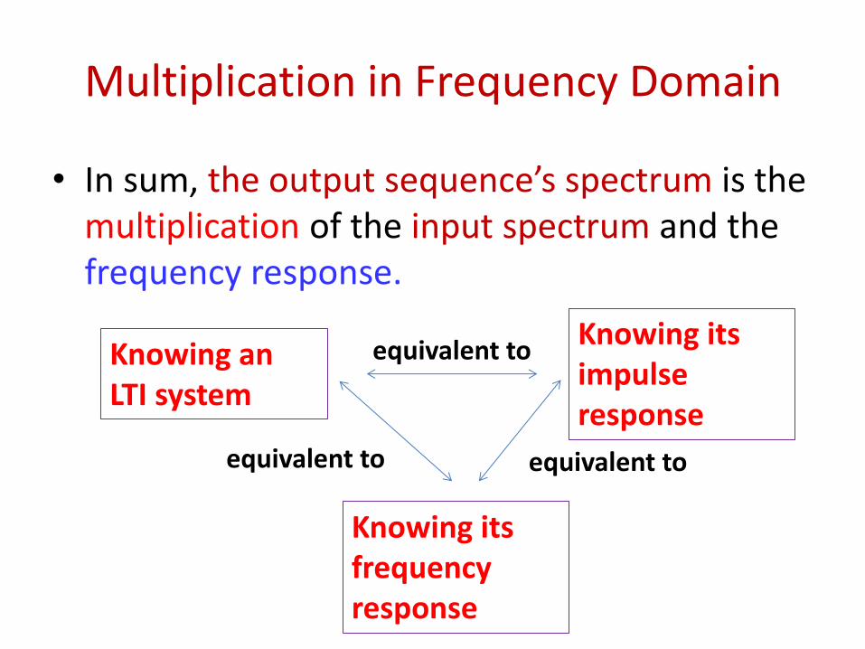
• In sum, the output sequence’s spectrum is the multiplication of the input spectrum and the frequency response.

Knowing an LTI system

Knowing its impulse response

equivalent to

Knowing its frequency response

equivalent to equivalent to

• Sinusoidal responses of LTI systems:

– The response of x1[n] and x2[n] are

– 𝑦1 𝑛 =𝐴

2𝑒𝑗𝜙𝐻 𝑒𝑗𝑤0 𝑒𝑗𝑤0𝑛 =

𝐴

2𝐻 𝑒𝑗𝑤 𝑒𝑗(𝑤0𝑛+𝜙)

– 𝑦2 𝑛 =𝐴

2𝑒−𝑗𝜙𝐻 𝑒−𝑗𝑤0 𝑒−𝑗𝑤0𝑛 =

𝐴

2𝐻 𝑒−𝑗𝑤0 𝑒−𝑗(𝑤0𝑛+𝜙)

– The total response is y[n] = y1[n] + y2[n]

Application Example of Eigenfunctions

nxnxeeA

eeA

nwAnxnjwjnjwj

21000

22

cos

Impulse response of the moving-average system is

Therefore, the frequency response is

Example: Frequency Response of the

Moving-average System

otherwise0

1

121

21

MnMMMnh

2

1

1

1

21

M

Mn

jwnjwe

MMeH

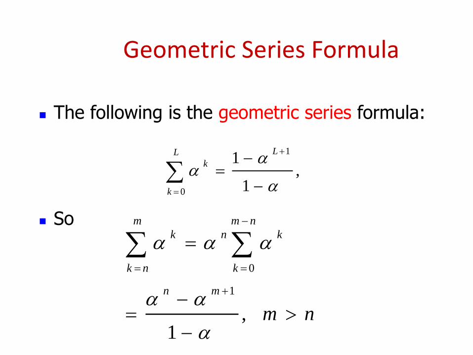
The following is the geometric series formula:

So

Geometric Series Formula

0

1

, 1

m m n

k n k

k n k

n m

m n

1

0

1,

1

LL

k

k

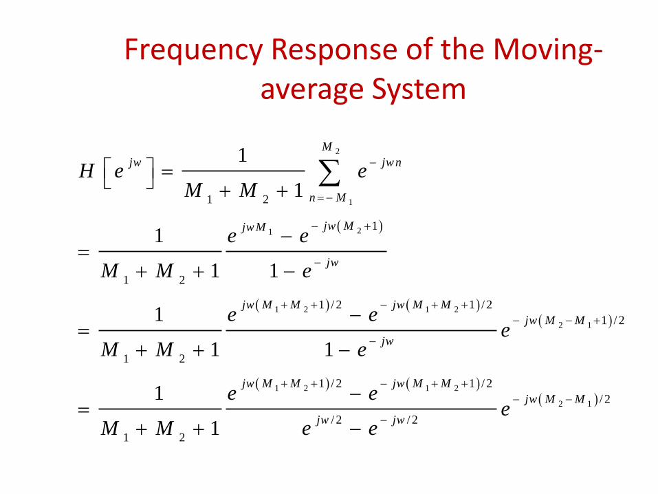
Frequency Response of the Moving-average System

2

1

21

1 2 1 2

2 1

1 2 1 2

2 1

1 2

1

1 2

1 / 2 1 / 2

1 / 2

1 2

1 / 2 1 / 2

/ 2

/ 2 / 2

1 2

1

1

1

1 1

1

1 1

1

1

M

jw jw n

n M

jw Mjw M

jw

jw M M jw M M

jw M M

jw

jw M M jw M M

jw M M

jw jw

H e eM M

e e

M M e

e ee

M M e

e ee

M M e e

Frequency Response of the Moving-average System

1 2 1 2

2 1

2 1

1 / 2 1 / 2

/ 2

/ 2 / 2

1 2

1 2 / 2

1 2

1

1

sin 1 / 21

1 sin / 2

expjw

jw M M jw M M

jw M Mjw

jw jw

jw M M

j H ejw

e eH e e

M M e e

w M Me

M M w

H e

(magnitude and phase)

Further evaluation

Spectrum of the Moving-average System (M1 = 0 and M2 = 4)

Recall that, in DTFT, the frequency response is repeated with period 2. “High frequency” is close to .

Amplitude response

Phase response

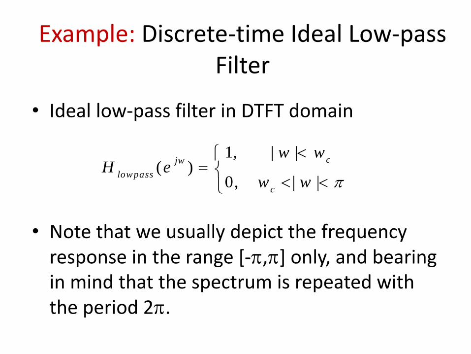
Example: Discrete-time Ideal Low-pass Filter

1, | |( )

0, | |

cjw

lowpass

c

w wH e

w w

• Ideal low-pass filter in DTFT domain

• Note that we usually depict the frequency response in the range [-,] only, and bearing in mind that the spectrum is repeated with the period 2.

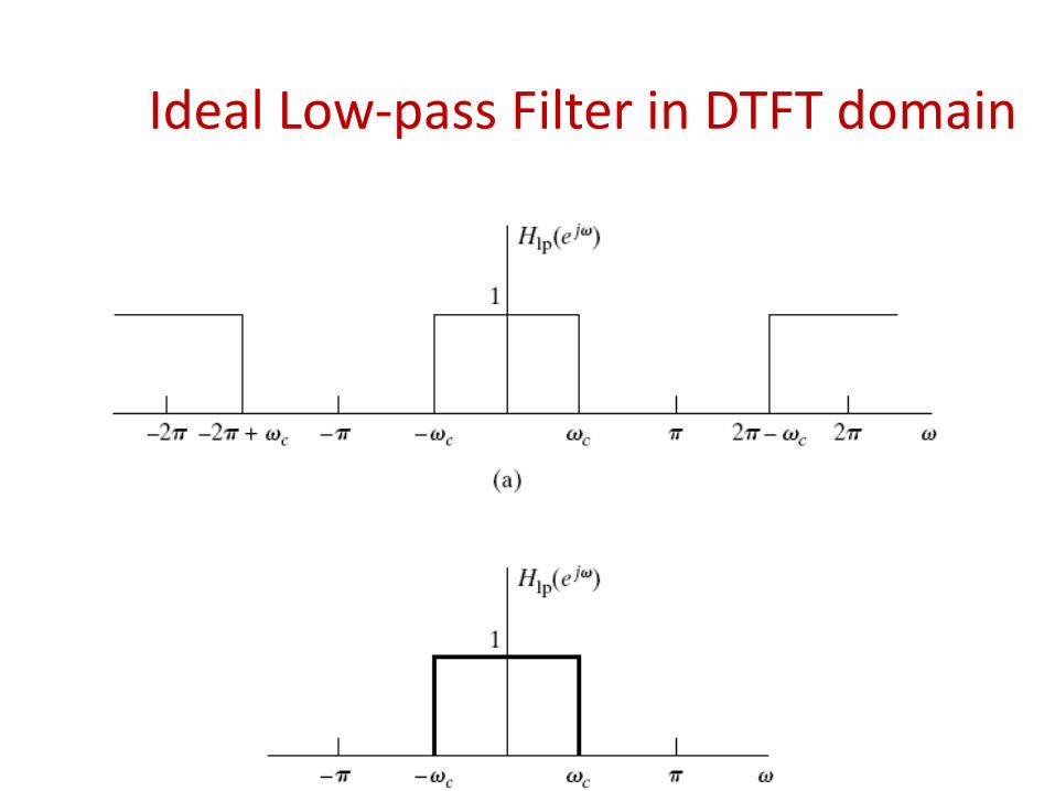
Ideal Low-pass Filter in DTFT domain

Discrete-time Ideal Low-pass Filter

• The impulse response hlowpass[n] can be found by inverse Fourier transform:

1

[ ]2

1 1| ( )

2 2

sin

c

c

c c c

c

wjw n

low passw

w jw n jw njw n

w

c

h n e dw

e e ejn jn

w n

n

Uniform samples of Sinc function

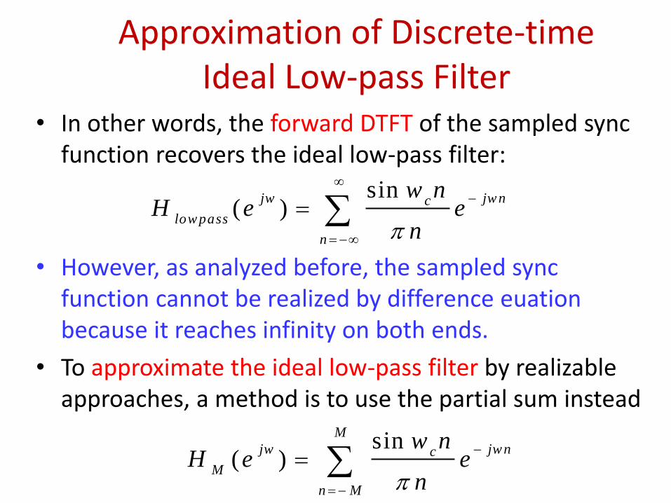
Approximation of Discrete-time Ideal Low-pass Filter

• In other words, the forward DTFT of the sampled sync function recovers the ideal low-pass filter:

• However, as analyzed before, the sampled sync function cannot be realized by difference euation because it reaches infinity on both ends.

• To approximate the ideal low-pass filter by realizable approaches, a method is to use the partial sum instead

sin( )

M

jw jw nc

M

n M

w nH e e

n

sin( )

jw jw nc

low pass

n

w nH e e

n

Approximation of Discrete-time Ideal Low-pass Filter

• Examples of M=1, 3, 7, 19

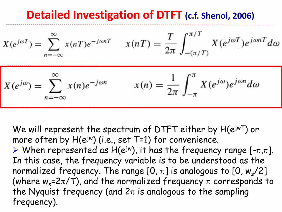
We will represent the spectrum of DTFT either by H(ejwT) or more often by H(ejw) (i.e., set T=1) for convenience. When represented as H(ejw), it has the frequency range [-,]. In this case, the frequency variable is to be understood as the normalized frequency. The range [0, ] is analogous to [0, ws/2] (where ws=2/T), and the normalized frequency corresponds to the Nyquist frequency (and 2 is analogous to the sampling frequency).

Detailed Investigation of DTFT (c.f. Shenoi, 2006)

DC response When w=0, the complex exponential ejw becomes a constant signal, and the frequency response X(ejw) is often called the DC response when w=0.

–The term DC stands for direct current, which is a constant current.

DTFT Properties Revisited

Time shifting

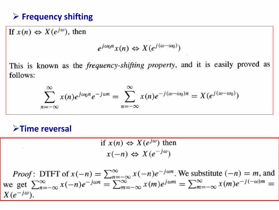
Frequency shifting

Time reversal

DTFT of (n)

DTFT of (n+k)+ (n-k)

According to the time-shifting property,

Hence

jwn

n

n

en

jwkjwkeknekn

is of DTFT , is of DTFT

wkeeknknjwkjwk

cos2 is of DTFT

10

jwe

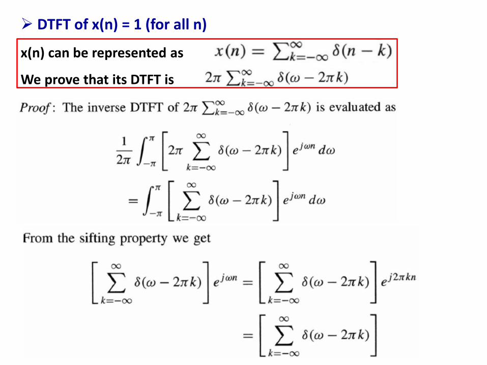
DTFT of x(n) = 1 (for all n)

x(n) can be represented as

We prove that its DTFT is

Hence

dwekwjwn

k

2

dwwdwwdwwdww

dwkw

k

2

ndww allfor 1

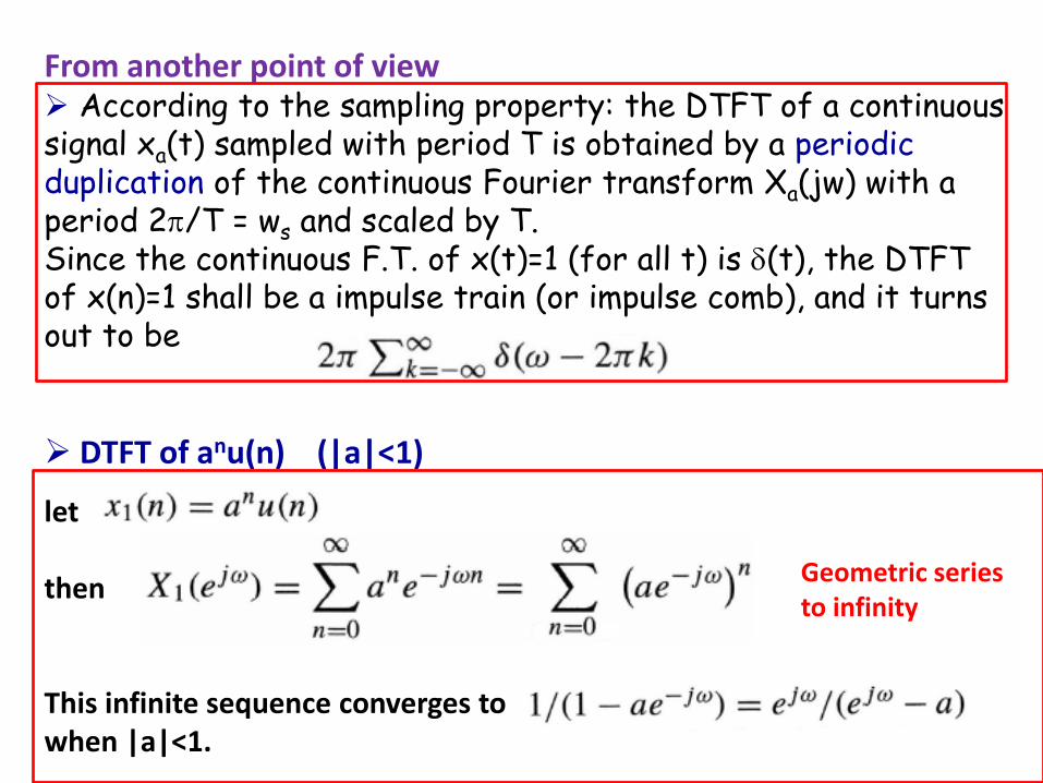
From another point of view According to the sampling property: the DTFT of a continuous signal xa(t) sampled with period T is obtained by a periodic duplication of the continuous Fourier transform Xa(jw) with a period 2/T = ws and scaled by T. Since the continuous F.T. of x(t)=1 (for all t) is (t), the DTFT of x(n)=1 shall be a impulse train (or impulse comb), and it turns out to be

DTFT of anu(n) (|a|<1)

let then This infinite sequence converges to when |a|<1.

Geometric series to infinity

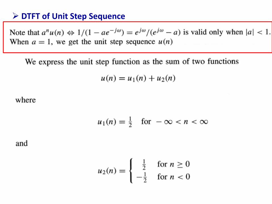
DTFT of Unit Step Sequence

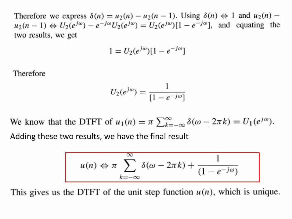
Adding these two results, we have the final result

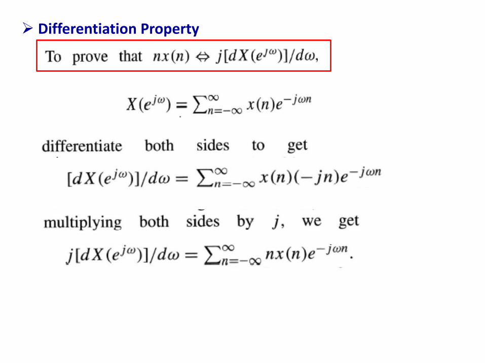
Differentiation Property

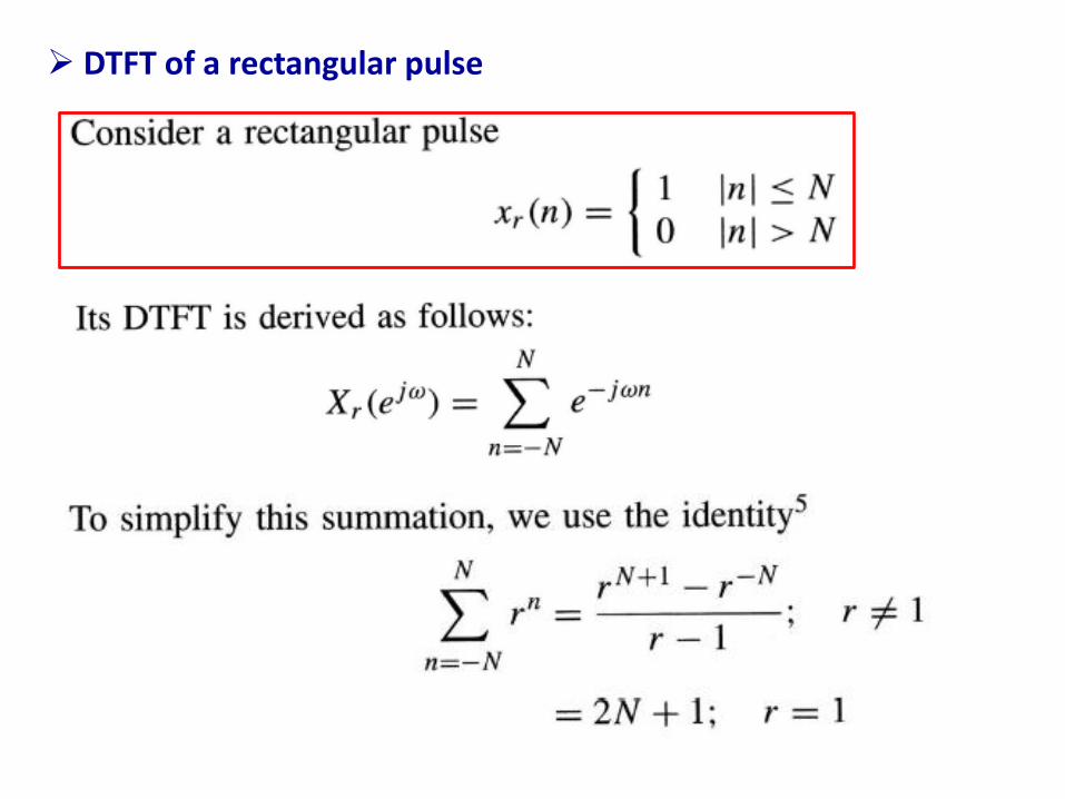
DTFT of a rectangular pulse

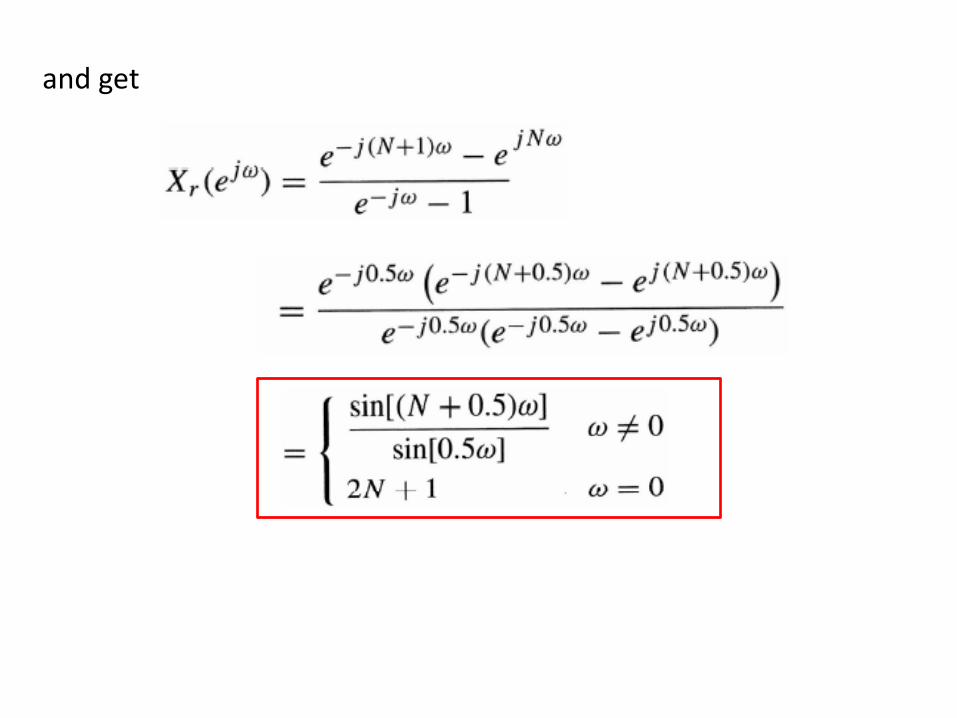
and get