
Research Report: Identification of major economic drivers ...
Economic Drivers of Mineral Supply
U.S. Geological Survey Open-File Report 02-335
Lorie A. Wagner, Daniel E. Sullivan, and John L. Sznopek
With an Introduction to the Series by Eric E. Rodenburg
Part of a multi-chapter study titled “The Meaning of Scarcity in the 21st Century”
U.S. Geological Survey
1

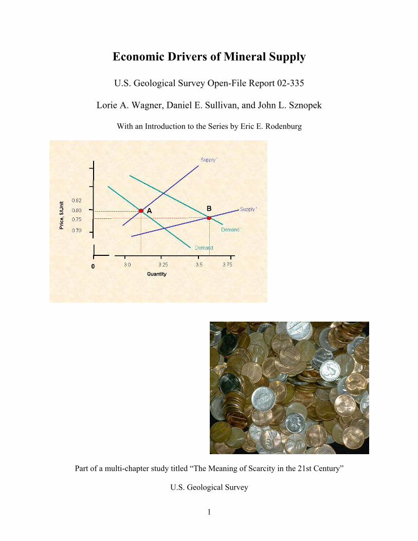
On the cover:
Supply – demand relation
Photograph of coins (Brøderbund Software, Inc., 1997)
2
CONTENTS Introduction to the series 8 Abstract 12 Introduction to the study 13 Economic drivers of mineral supply 15 Sidebar: What are constant dollars? 18
Use 19 Historical minerals use in the United States 20 Sidebar: Consumption and use of materials 25 Resources and reserves 28 Sidebar: Resource, reserve base, and reserve definitions 29 Supply-demand relation theory 36 Sidebar: Prices and exploration for new mines 41 Sidebar: The molybdenum story – creation of markets and price changes and
the Climax Mine 44 Price 54
Sidebar: Prices and closing mines 56 Sidebar: Higher silver prices and increased recycling 58 Historical prices 61
Production 64 Sidebar: Mercury’s declining production 64 Sidebar: Favorable political and economic factors required in recovering mineral deposits – Congo (Kinshasa) 67 Historical production 69
Globalization 71 Historical imports and exports in the United States 72 Sidebar: Globalization of the aluminum industry 79 Technology and productivity 81 Historical productivity 84 Sidebar: Technology and productivity in the copper industry 87 Production costs 89 Capital costs 92 Strategies for efficient materials usage 94
Sidebar: The copper penny 96 Summary 97 References 100
Appendix A – Supply – demand relation theory 105 Appendix B – Prices 114 Appendix C – Production 152 Appendix D – Economic case study - Aluminum 180 Appendix E – Economic case study - Copper 209 Appendix F – Economic case study - Potash 232 Appendix G – Economic case study - Sulfur 251
3

FIGURES 1. The role of nonfuel minerals in the U.S. economy for the year 2000 16 2. Value of nonfuel mineral production in the United States in constant 2000 dollars,
1950-2000 17 3. Renewable and nonrenewable materials used in the United States, 1900-2000 21 4. U.S. flow of raw materials by weight, 1900-2000 22 5. U.S. flow of raw materials by weight, 1950 and 2000 23 6. Major elements of mineral-resource classification, excluding reserve base and
inferred reserve base 30 7. Reserve base and inferred reserve base classification categories 31 8. Demand curve 38 9. Supply curve 40 10. Distribution of mineral exploration budgets in the year 2000, by commodity
grouping 42 11. Supply-demand curve showing the equilibrium point 43 12. U.S. molybdenum concentrate production and price, 1900-2000 45 13. U.S. exports and imports of molybdenum ores and concentrates, 1918-2000 47 14. U.S. and world production of molybdenum concentrate, 1900-2000 50 15. U.S. apparent consumption of molybdenum, 1900-2000 51 16. U.S. stocks of molybdenum, 1941-2000 53 17. U.S. silver price, in constant 2000 dollars per troy ounce (yearly average),
1900-2000 59 18. U.S. silver production from old scrap versus price, in constant 2000 dollars,
1974-84 60 19. U.S. mine production composite price index, in 2000 constant dollars, 1905-2000 62 20. U.S. composite mine mineral production index, 1906-2000 70 21. Total U.S. imports and exports in constant 2000 dollars, 1971-2000 72 22. U.S. net import reliance for selected nonfuel mineral materials, 2000 74 23. U.S. imports of mineral raw materials, 1978-2000 76 24. U.S. imports of mineral raw materials as percent of total U.S. imports
(value based), 1978-2000 77 25. U.S. mineral price index, in constant 2000 dollars, versus U.S. consumption
of raw materials, 1900-2000 78 26. U.S. aluminum trade data and apparent consumption, 1900-2000 81 27. U.S. mining industries labor productivity indexes, 1947-97 85 28. U.S. stone, clay, glass, and concrete products productivity indexes, 1949-98 86 29. U.S. copper industry labor productivity index, 1955-98 88 30. U.S. mineral price index, in constant 2000 dollars, versus U.S. consumption
of raw materials, 1900-2000 97 Appendix A. Supply – demand relation A1. The competitive price system 105 A2. Hypothetical supply-demand situation for copper 108 A3. Equilibrium price and quantity changes as a result of shifts in supply and demand 110 A4. Equilibrium price or quantity impacts of supply or demand increases 112
4
Appendix B. Prices B1. U.S. mine production composite price index, in constant 2000 dollars, 1905-2000 116 B2. U.S. industrial minerals price index, in constant 2000 dollars, 1905-2000 131 B3. U.S. cement price, in constant 2000 dollars, 1900-2000 132 B4. U.S. clay price, in constant 2000 dollars, 1900-2000 133 B5. U.S. lime price, in constant 2000 dollars, 1904-2000 134 B6. U.S. phosphate rock price, in constant 2000 dollars, 1900-2000 135 B7. U.S. salt price, in constant 2000 dollars, 1900-2000 136 B8. U.S. sand and gravel price, in constant 2000 dollars, 1902-2000 137 B9. U.S. crushed stone price, in constant 2000 dollars, 1905-2000 138 B10. U.S. metal price index, in constant 2000 dollars, 1900-2000 140 B11. U.S. copper price, in constant 2000 dollars, 1900-2000 141 B12. U.S. gold price, in constant 2000 dollars, 1900-2000 143 B13. U.S. mine production composite price index excluding gold, in constant 2000 dollars, 1905-2000 144 B14. U.S. iron ore price, in constant 2000 dollars, 1900-2000 145 B15. U.S. lead price, in constant 2000 dollars, 1900-2000 146 B16. U.S. zinc price, in constant 2000 dollars, 1900-2000 147 B17. U.S. aluminum price, in constant 2000 dollars, 1900-2000 149 Appendix C – Production C1. U.S. composite mineral production index, 1906-2000 161 C2. U.S. industrial mineral production index, 1904-2000 162 C3. U.S. cement production, 1900-2000 163 C4. U.S. clay production, 1900-2000 164 C5. U.S. lime production, 1904-2000 165 C6. U.S. phosphate rock production, 1900-2000 166 C7. U.S. salt production, 1900-2000 167 C8. U.S. sand and gravel production, 1902-2000 168 C9. U.S. crushed stone production, 1900-2000 169 C10. U.S. metal mine production index, 1906-2000 170 C11. U.S. copper mine production, 1900-2000 171 C12. U.S. gold mine production, 1900-2000 173 C13. U.S. iron ore production, 1900-2000 174 C14. U.S. lead mine production, 1906-2000 175 C15. U.S. zinc mine production, 1900-2000 176 C16. U.S. aluminum metal production, 1900-2000 177 Appendix D – Aluminum case study D1. U.S aluminum flow diagram 182 D2. U.S. aluminum price, in constant 2000 dollars, 1900-2000 184 D3. U.S. Bauxite price, in constant 2000 dollars, and world production, 1900-2000 185 D4. U.S. production of alumina, bauxite, and primary aluminum, 1900-2000 188 D5. U.S. primary and secondary (old) aluminum production, 1900-2000 190 D6. World production of alumina, bauxite, and primary aluminum, 1900-2000 191
5
D7. U.S. primary aluminum production as a percent of world production, 1900-2000 192 D8. U.S. apparent consumption of alumina, aluminum and bauxite, 1900-2000 195 D9. U.S. distribution of end-use shipments of aluminum products, 1980-2000 196 D10. U.S. bauxite imports and exports, 1900-2000 198 D11. U.S. alumina imports, exports, and production, 1935-2000 199 D12. U.S. aluminum imports and exports, 1911-2000 200 D13. U.S. aluminum productivity and number of aluminum industry employees, 1964-2000 202 Appendix E – Copper case study E1. U.S. copper price, in constant 2000 dollars, 1900-2000 210 E2. U.S. copper mine production, copper content, 1900-2000 211 E3. U.S. copper price, in constant 2000 dollars, compared to mine production, 1900-2000 213 E4. U.S. copper refinery production, copper metal, 1900-2000 214 E5. U.S. copper refinery production by source, by percent, 1900-2000 215 E6. World copper mine production, copper content, 1900-2000 216 E7. U.S. share of world copper mine production, by percent, copper content, 1900-2000 217 E8. U.S. apparent consumption of copper metal, 1900-2000 220 E9. U.S. apparent consumption of copper, in terms of metric tons per capita, 1900-2000 221 E10. U.S. net imports of refined copper metal, thousand metric tons, 1900-2000 222 E11. U.S. copper mining labor productivity index from the Bureau of Labor Statistics, output per hour, 1955-98 223 Appendix F – Potash case study F1. U.S. potash average price, in constant 2000 dollars, 1922-2000 234 F2. U.S. potash mine production, 1915-2000 235 F3. U.S. potash price, compared to U.S. mine production, 1920-2000 237 F4. World potash mine production, 1920-2000 238 F5. U.S. share of world potash mine production, 1921-2000 239 F6. U.S. apparent consumption of potash, 1905-2000 241 F7. U.S. apparent consumption of potash per capita, 1924-2000 242 F8. U.S. imports of potash, 1905-2000 243 F9. U.S. exports of potash, 1937-2000 244 F10. U.S. net imports of potash, 1905-2000 245 Appendix G – Sulfur case study G1. U.S sulfur flow diagram 252 G2. U.S. sulfur price, in constant 2000 dollars, 1900-2000 256 G3. U.S sulfur production trends, 1900-2000 259 G4. World sulfur production, 1940-2000 261 G5. World byproduct sulfur production, 1989-2000 262 G6. U.S. sulfur production as a percent of world sulfur production, 1940-2000 263 G7. U.S. apparent consumption of sulfur, 1900-2000 265
6
G8. End use of sulfur and sulfuric acid in the United States, 1975-2000 267 G9. U.S. elemental sulfur imports and exports, 1900-2000 269 G10. U.S sulfur productivity and number of sulfur industry employees, 1955-2000 270 TABLES 1. Copper resource, reserve base, and reserve estimates for the year 2001 33 2. World copper reserves 35 3. Value of nonfuel mineral production in the United States in the year 2000 63 4. 1997 mining costs, in thousand dollars 90 Appendix B – Prices B1. Value of nonfuel mineral production in the United States in the year 2000 117 B2. Prices of selected mineral commodities in current dollars 118 B3. Prices of selected mineral commodities in constant dollars 123 B4. Consumer price index, 2000 = 100 128 B5. Price indexes, in constant 2000 dollars 129 Appendix C – Production C1. Production of selected mineral commodities, in thousand tons, unless otherwise noted 154 C2. Production indexes, 2000 = 100 159 Appendix D – Aluminum case study D1. Bauxite reserves and reserve base estimates, in million tons 194 D2. Domestic primary aluminum industry data 203 Appendix E – Copper case study E1. Production costs for U.S copper mining industry in 1997 225 Appendix F – Potash case study F1. Unit price of potash, in dollars per ton 233 F2. Domestic production of potash, in tons 236 F3. Production costs for potash, soda, and borate mineral mining industry in 1997 247 Appendix G – Sulfur case study G1. Price of sulfur, in dollars per ton 255 G2. Domestic production of sulfur, in thousands of tons 258 G3. Sulfur reserves and reserve base estimates, in million tons of sulfur 264
7
INTRODUCTION TO THE SERIES1
The possibility of future mineral scarcity is an important concern of environmental activists,
those desiring to limit population growth, and those concerned with wealth distribution between
industrialized and developing countries. Through the years, observers from Thomas Malthus
(1798) to the 1972 Club of Rome report, (Meadows and others, 1972), for example, predicted
exhaustion of resources at various dates, most of which have come and gone without the dire
consequences of societal collapse they envisioned.
The static model from which these predictions came continues to inform many who choose to
believe that mineral production cannot meet the material aspirations of a rapidly growing world
population if consumption (one component of which is resource capitalization, which is often
overlooked by these analysts) of some resources continues to increase. The perception of future
scarcity, for example, motivated the Factor Ten Club, a group of resource economists, to issue
the Carnoules Declaration in 1994 and 1995. The Declarations called for a swift 10-fold increase
in material efficiency among industrialized countries to free materials for people in developing
countries (Factor 10 Club, 1995).
The concerns of future scarcity may in part be caused by misinterpretation and (or) the misuse of
published mineral reserve estimates for non-fuel mineral commodities. A reserve is that part of
an in-place demonstrated resource that can be economically extracted or produced at the time of
estimation (U.S. Bureau of Mines and U.S. Geological Survey, 1980). Some misinterpret the
1 Introduction to the series was written by Eric E. Rodenburg, Chief, Minerals and Materials Analysis Section, U.S. Geological Survey.
8
term “reserve” as an estimate of all-that-is-left.
Mineral supply starts with the physical existence of materials, and can be no greater than its
occurrence in the Earth’s crust. The amount of material actually supplied to society (economic
supply) is that which is called forth by demand (willingness-to-pay), as moderated by the cost of
production, which is influenced by physical realities, technology, politics, and social concerns.
In fact, many of the minerals that the Earth’s population demands exist in nearly inexhaustible
amounts. Additionally, there is an enormous stock of resources in materials in-use (machinery,
buildings, and roads) and in unutilized waste (landfills). There is, however, a growing
understanding that physical scarcity is not the only, or even the most, important issue. Industrial
activities extract and transform resources into products people use. In many cases, these
activities come with direct or accumulative environmental consequences that can pose serious
threats to ecosystems and human health. Thus, the important issue of scarcity may be the
capacity of Earth’s geologic, hydrologic, and atmospheric systems to assimilate the wastes
(Meadows and others, 1972).
This series, “Scarcity in the 21st Century”, addresses resource constraints and opportunities, and
the effects of their interactions on resource supply. Assessing potential supply requires a whole
systems approach, both in physical terms by looking at the flows of materials through the
economy, and in human terms by integrating the interactive domains of economics, environment,
policy, technology, and societal values.
9
In 1929, D.F. Hewett, of the United States Geological Survey (USGS), reflecting on the effects
of war on metal production, identified four factors he deemed most important in influencing
metal production (Hewett, 1929).
1. Geology
“First, there are the geological factors, which are concerned with the minerals
present; their number and kind, which determine whether the problem of recovery
is simple or complex; the degree of their concentration or dissemination; their
border relations; the shape and extent of the recognizable masses.”
2. Technology
“Second, there are the technical factors of mining, treatment and refining. A
review of these leaves a vivid impression of the labor involved in their
improvement but they necessarily yield cumulative benefits.”
3. Economics
“The third group of factors that affects rates of production are economic, and
among these factors cost and selling price are outstanding... Since 1800 the trend
of prices for the common metals, measured not only by monetary units but by the
cost in human effort, has been almost steadily downward…”
4. Politics
“The fourth group of factors that affect metal-production curves are political or lie
between politics and economics.”
10
The four factors do not operate separately, but rather as parts of an integrated system, which also
includes social constraints and drivers such as environmental issues and the structure of the
mining industry.
“Scarcity in the 21st Century” is composed of six chapters to be published in a series of USGS
Open File Reports and then compiled as a USGS Circular.
Chapter 1: “The Supply of Materials” examines the physical supply of minerals on the planet, in
the ground and products-in-use, waste streams, and waste deposits (landfills). Current and future
potential for recycling of products-in-use and landfill materials are examined.
Chapter 2: “Economic Drivers of Mineral Supply” explores price, investment, costs, and
productivity, and their relevance to supply.
Chapter 3: “Technological Advancements – A Factor in Increasing Resource Use” investigates
the impact of technological change on mineral extraction, processing, use and substitution.
Chapter 4: “Social Constraints and Encouragement to Mineral Supply” addresses social realities
that affect mineral supply, nationally and globally, and the socio-cultural trends that promise to
have an impact on future supplies.
Chapter 5: “Policy – A Factor Determining the Parameters of Minerals Supply and Demand”
examines the effect of government policies that either promote or restrain mineral development,
11
some of which include: access, title, regulation, rent, royalty, and tax fees, and direct and indirect
subsidies. This chapter also discusses the affects of corporate policies on mineral supply.
Chapter 6: “Overview of Minerals Supply” presents an overall view of these parameters of
supply to show their synergy in supply and ultimately production.
Each chapter contains ample reference to historical information about one or more commodities
to illustrate the concepts.
ABSTRACT
The debate over the adequacy of future supplies of mineral resources continues in light of the
growing use of mineral-based materials in the United States. According to the U.S. Geological
Survey, the quantity of new materials utilized each year has dramatically increased from 161
million tons2 in 1900 to 3.2 billion tons in 2000. Of all the materials used during the 20th
century in the United States, more than half were used in the last 25 years.
With the Earth’s endowment of natural resources remaining constant, and increased demand for
resources, economic theory states that as depletion approaches, prices rise. This study shows
that many economic drivers (conditions that create an economic incentive for producers to act in
a particular way) such as the impact of globalization, technological improvements, productivity
increases, and efficient materials usage are at work simultaneously to impact minerals markets
2 In this report, all tons are metric tons unless otherwise noted.
12
and supply. As a result of these economic drivers, the historical price trend of mineral prices3 in
constant dollars has declined as demand has risen. When price is measured by the cost in human
effort, the price trend also has been almost steadily downward.
Although the United States economy continues its increasing mineral consumption trend, the
supply of minerals has been able to keep pace. This study shows that in general supply has
grown faster than demand, causing a declining trend in mineral prices.
INTRODUCTION TO THE STUDY
The objective of this study is to analyze the main economic drivers that prompt producers to
either supply more or less mineral-based materials to the market. Economic drivers are those
conditions that create an economic incentive for producers to act in a particular way.
Price is an example of an economic driver because, as prices rise, producers supply more
mineral-based materials to the market. Price may be the most important economic driver since
other economic drivers such as production costs and the impacts of globalization, influence
price. This study builds upon research conducted previously (Sullivan, Sznopek, and Wagner,
2000) that analyzed the long-term trend of mineral prices in the United States.
An almost endless list of factors could be considered economic drivers because in one-way or
3 All historical mineral prices in this study are from U.S. Geological Survey Open-File Report 01-006 where they are referred to as unit value. For a complete explanation of unit value, please refer to the methodology section of OFR 01-006 at URL http://minerals.usgs.gov/minerals/pubs/of01-006/.
13
another these factors can impact the supply-demand curve. These factors include people’s
perceptions of the economy, current events, political activities, population and factors such as the
weather. Governmental actions in the form of taxes, environmental regulations, and
governmental spending also can greatly influence the decisions producers make regarding the
amount of material to be supplied to the market. These factors are complex, take place
simultaneously, and interact with one another. This study addresses the major economic factors
that influence the amount of material supplied to the market. Other chapters in this series
“Scarcity in the 21st Century” address additional factors.
Chapter 1: “The supply of materials” examines the physical endowment of minerals.
Chapter 3: “Technological advancements - A factor in increasing resource use”
addresses the impact of technological change.
Chapter 4: “Mineral supply - Sociocultural drivers and constraints” addresses the social
realities that affect mineral supply.
Chapter 5: “Policy – A factor determining the parameters of mineral supply and
demand” examines the effect of government policies including regulation, rents/royalties,
subsidies, and taxes.
Chapter 6: “Overview of minerals supply” brings together these parameters of supply to
show their synergy in supply and ultimately production.
These chapters present additional information on factors which influence the amount of
material supplied to the market.
This report shows the supply of minerals in the United States has been sufficient to meet the
increasing consumption trend of the U.S. economy. The historical trend of mineral prices in
14

constant dollars continues to decline due to the impact of efficient materials use, globalization,
productivity increases, and technological improvements.
In this report, trends in material use and resources and reserves are discussed first. Then the
basic principles of the supply-demand relation theory follow to support the subsequent
discussion regarding economic drivers such as price, production, globalization, technology and
productivity, production costs, capital costs, and strategies for efficient materials use. More
detailed discussion of the theory of the supply-demand relation, price indices and prices, and
production indices and production levels is presented in Appendices A, B, and C, respectively.
Case studies describing the economic drivers for the commodities aluminum, copper, potash, and
sulfur are presented in Appendices D, E, F, and G, respectively.
ECONOMIC DRIVERS OF MINERAL SUPPLY
Economic activity is one way human beings provide for their material requirements, including
both basic necessities and additional items that make life more enjoyable. Mineral-based
materials play a vital role in the economy of the United States and the world. The value of
domestic production of mineral raw materials from mining was estimated at $40 billion in 2000,
while the value of old scrap4 reclaimed in this same year was estimated at $10 billion (U.S.
Geological Survey, 2001a, p. 4). As shown in figure 1, these raw materials are processed
domestically to produce aluminum, brick, cement, copper, fertilizers, steel, and other products.
Shipments of processed nonfuel minerals in the United States in the year 2000 were valued at
4 Old scrap is the term used for products that have reached the end of their economic life and are discarded and then enter back into the system as material available for recycling.
15
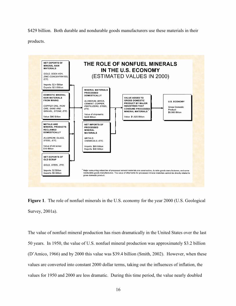
$429 billion. Both durable and nondurable goods manufacturers use these materials in their
products.
*
*
Figure 1. The role of nonfuel minerals in the U.S. economy for the year 2000 (U.S. Geological
Survey, 2001a).
The value of nonfuel mineral production has risen dramatically in the United States over the last
50 years. In 1950, the value of U.S. nonfuel mineral production was approximately $3.2 billion
(D’Amico, 1966) and by 2000 this value was $39.4 billion (Smith, 2002). However, when these
values are converted into constant 2000 dollar terms, taking out the influences of inflation, the
values for 1950 and 2000 are less dramatic. During this time period, the value nearly doubled
16
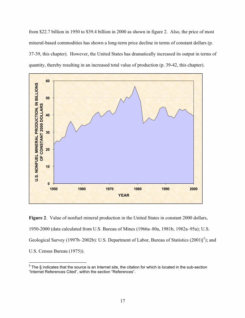
from $22.7 billion in 1950 to $39.4 billion in 2000 as shown in figure 2. Also, the price of most
mineral-based commodities has shown a long-term price decline in terms of constant dollars (p.
37-39, this chapter). However, the United States has dramatically increased its output in terms of
quantity, thereby resulting in an increased total value of production (p. 39-42, this chapter).
0
10
20
30
40
50
60
1950 1960 1970 1980 1990 2000YEAR
U.S
. NO
NFU
EL M
INER
AL
PRO
DU
CTI
ON
, IN
BIL
LIO
NS
OF
CO
NST
AN
T 20
00 D
OLL
AR
S
Figure 2. Value of nonfuel mineral production in the United States in constant 2000 dollars,
1950-2000 (data calculated from U.S. Bureau of Mines (1966a–80a, 1981b, 1982a–95a); U.S.
Geological Survey (1997b–2002b): U.S. Department of Labor, Bureau of Statistics (2001§5); and
U.S. Census Bureau (1975)).
5 The § indicates that the source is an Internet site, the citation for which is located in the sub-section “Internet References Cited”, within the section “References”.
17
What Are Constant Dollars?
The dollar you use to buy something today looks like the dollar that you spent last year or the
one you spent 20 years ago, but it is not the same. The loaf of bread that you can currently buy
for a dollar may have cost 95 cents last year and 50 cents 20 years ago. Thus the dollar that you
had 20 years ago would have purchased two loaves of bread at that time. The basket of groceries
that you purchased last year for $57 currently costs you $60. What has happened to the dollar?
Why does it purchase less today than it did in the past?
What happened is called inflation. Inflation is an increase in the general level of prices and an
erosion of the purchasing power of the dollar. Both inflation (increasing prices) and deflation
(decreasing prices) are possible. However moderate inflation has been the prevailing trend in
our modern economy since World War II.
Constant dollars are dollars in which the effects of changes in the purchasing power of today’s
dollar (current dollars) over time have been removed. Analysts have developed price indexes to
estimate constant dollars. Price indexes estimate the relative changes in average prices over
time.
This analysis uses the Consumer Price Index (CPI) to estimate constant dollars. The CPI utilizes
changes in the average prices of a market basket of goods to estimate changes in the value of a
dollar. The market basket is designed to be a representative sample of goods purchased. The
18
What Are Constant Dollars?Continued
CPI can be used to estimate how many of today’s dollars it would have cost to purchase a loaf of
bread or some other item in past years. Constant dollars are in comparable terms over time.
Thus we can compare the real prices of a good at different time periods.
Historical trends of some of the factors that affect the amount of material supplied are important
trends to be examined. The historical time series identifies long-term trends and can indicate
possible future scenarios regarding the supply of minerals. Analyzing historical data is
important, as it can reveal how past supply shortages have been overcome, or diverted. It can
also show how the economic system can work to reduce the possibility of future resource
scarcity.
Use
Before a mineral can attain any value, it needs to be located, extracted, and converted into usable
products for which a demand exists, and delivered to consumers in the required quantities and
qualities at the needed times and locations. Demand for minerals stimulates their supply.
Demand is the relation between the various possible prices of a product and the amounts of it
that consumers are willing and able to buy during some period of time, other economic factors
remaining the same. It is important to note the “willing and able to buy” concept is different
from a consumer’s wants and needs. A consumer’s desire or willingness to purchase a product
has no impact on demand if the consumer does not have the purchasing power to buy the
19
product. In many cases, consumption (or use) is a proxy for demand because products were
actually purchased by the consumer.
Supply occurs to meet current and anticipated demand. In theory, if there is no demand for a
material, the supply will be zero. When demand increases, prices tend to rise and/or producers
supply more goods to the market to keep up with the rising demand. When demand increases
faster than supply, temporary shortages exist6. When supply increases faster than demand,
excess supply in the form of stockpiles can become an issue.
Historical minerals usage in the United States
Food, fuel, and materials are three broad categories of commodities used in the economy to
support the requirements of society. The following section from Matos and Wagner, 1998,
examines the historical usage of mineral-based materials since 1900. The mineral-based
materials of metal and industrial mineral commodities like cement and sand and gravel are
examined.
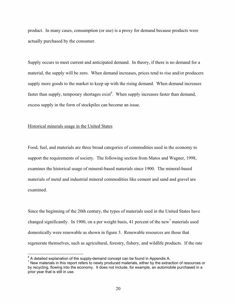
Since the beginning of the 20th century, the types of materials used in the United States have
changed significantly. In 1900, on a per weight basis, 41 percent of the new7 materials used
domestically were renewable as shown in figure 3. Renewable resources are those that
regenerate themselves, such as agricultural, forestry, fishery, and wildlife products. If the rate
6 A detailed explanation of the supply-demand concept can be found in Appendix A. 7 New materials in this report refers to newly produced materials, either by the extraction of resources or by recycling, flowing into the economy. It does not include, for example, an automobile purchased in a prior year that is still in use.
20
they are harvested becomes so great that it drives the resource to exhaustion or extinction,
however, renewable resources can become nonrenewable. In contrast, nonrenewable resources
typically form over long periods of geologic time. They include metals, industrial minerals, and
organic materials (such as fossil-fuel-derived materials).
0
10
20
30
40
50
60
70
80
90
100
1900 1910 1920 1930 1940 1950 1960 1970 1980 1990 2000
YEAR
PER
CEN
TAG
E O
F TO
TAL
MA
TER
IALS
USE
D, O
N A
PER
-WEI
GH
T B
ASI
S Nonrenewable materials
Renewable materials
Figure 3. Renewable and nonrenewable materials used in the United States, 1900-2000
(Wagner, 2002).
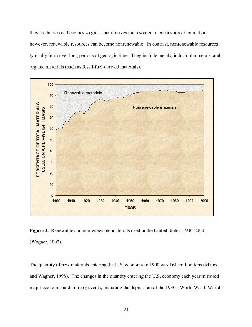
The quantity of new materials entering the U.S. economy in 1900 was 161 million tons (Matos
and Wagner, 1998). The changes in the quantity entering the U.S. economy each year mirrored
major economic and military events, including the depression of the 1930s, World War I, World
21
War II, the post-World War II boom, the ‘oil crisis’ of the 1970s, and the recession of the 1980s
as shown in figure 4. During this time frame, the U.S. economy moved rapidly from an
agricultural to an industrial base. In the 1950s and 1960s, it started to shift toward a service
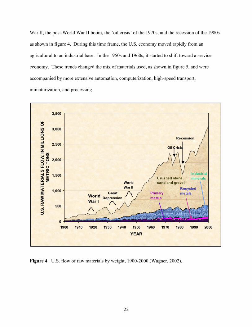
economy. These trends changed the mix of materials used, as shown in figure 5, and were
accompanied by more extensive automation, computerization, high-speed transport,
miniaturization, and processing.
0
500
1,000
1,500
2,000
2,500
3,000
3,500
1900 1910 1920 1930 1940 1950 1960 1970 1980 1990 2000
YEAR
U.S.
RAW
MAT
ERIA
LS F
LOW
, IN
MIL
LIO
NS O
F M
ETRI
C TO
NS
Industrial minerals
Recycled metalsPrimary
metalsWorld War I
World War II
Great Depression
Oil Crisis
Recession
Crushed stone, sand and gravel
Figure 4. U.S. flow of raw materials by weight, 1900-2000 (Wagner, 2002).
22
Metals
2000
5%4%4%12%
75%Crushed stone,
sand and gravel
Industrial minerals
MetalsNonrenewable
organics
Agricultural and forest products
1950
10%3%
8%17%
62%Crushed stone,
sand and gravel
Industrial minerals
Nonrenewable organics
Agricultural and forest products
Figure 5. U.S. flow of raw materials by weight, 1950 and 2000 (Wagner, 2002).
By the end of the 20th century, only 5 percent of the 3,400 million tons of new materials entering
the U.S. economy in 2000 were renewable whereas 41 percent of the 161 million tons were
renewable in 1900. Of all the materials used during this century in the United States, more than
half were used in the last 25 years. More details on the data and trends of materials usage in the
United States are presented in Matos and Wagner (1998, p.109-113).
Crushed stone and construction sand and gravel make up as much as three quarters (by weight)
of new resources used annually. Use of these materials greatly increased as a result of
23

infrastructure growth (especially the interstate highway system) after World War II. In recent
decades, construction materials have been used mainly in building new suburban complexes,
widening and rebuilding roads damaged from weather and heavy traffic loads, and in
construction of bridges, ramps, and buildings.
Other industrial mineral commodities account for the next largest share of materials use. These
include cement for concrete; potash and phosphate for fertilizer; gypsum for drywall and plaster;
fluorspar for acid; soda ash for glass and chemicals; and sulfur, abrasives, asbestos, and other
minerals used for products and manufacturing processes.
On a percentage basis, the use of metals, by weight, declined slightly relative to other materials.
Reasons for this include the desire for lighter-weight materials (such as aluminum), the
introduction of high-strength, low-alloy steel in vehicles, and the availability of substitute
materials such as plastics.
Improvements in recycling technologies, reduced recycling costs, and increased consumer
preferences for environmentally friendly products have resulted in the growth of recycling of
metals and industrial mineral commodities, such as concrete. The sudden emergence of recycled
metals, shown in figure 4, in the 1960s reflects data disaggregation. Before the 1960s, recycled
metals were included in total metals values. According to 2000 estimates, 62.1 percent of all
aluminum beverage cans were recycled (Aluminum Association, Inc., 2001§). The 2000
recycling rates for steel-containing products were 84.1 percent for appliances, 95.0 percent for
automobiles, and 58.4 percent for steel cans (Steel Recycling Institute, 2001§). As a result of
24
this level of recycling of iron and steel, 55 percent of the requirement for iron and steel is met by
recycled sources (Fenton, 2002, p. 63.14). This means that 74 million tons less material
comprising iron and steel was produced from primary (virgin) sources.
Consumption and Use of Materials
From Wagner, 2002, p. 5
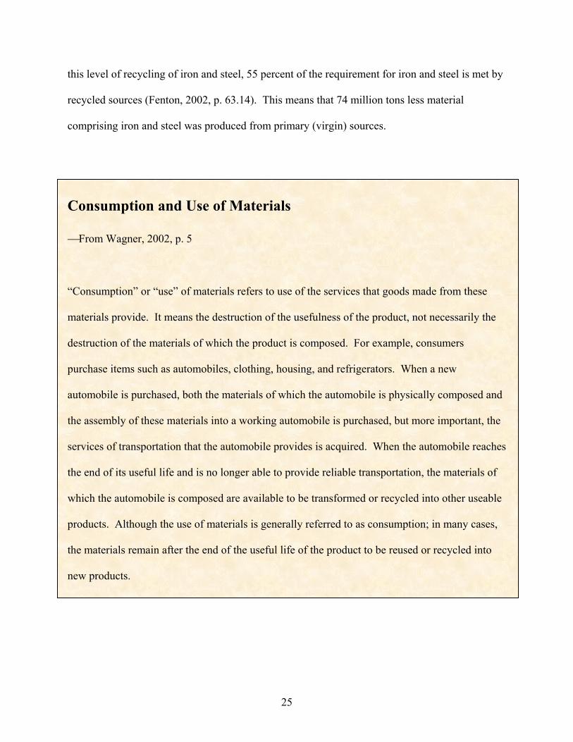
“Consumption” or “use” of materials refers to use of the services that goods made from these
materials provide. It means the destruction of the usefulness of the product, not necessarily the
destruction of the materials of which the product is composed. For example, consumers
purchase items such as automobiles, clothing, housing, and refrigerators. When a new
automobile is purchased, both the materials of which the automobile is physically composed and
the assembly of these materials into a working automobile is purchased, but more important, the
services of transportation that the automobile provides is acquired. When the automobile reaches
the end of its useful life and is no longer able to provide reliable transportation, the materials of
which the automobile is composed are available to be transformed or recycled into other useable
products. Although the use of materials is generally referred to as consumption; in many cases,
the materials remain after the end of the useful life of the product to be reused or recycled into
new products.
25
Consumption and Use of MaterialsContinued
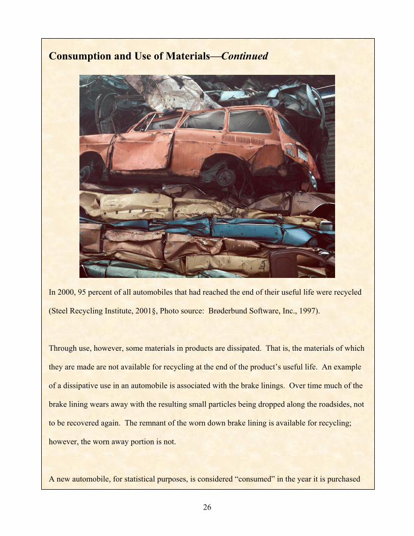
In 2000, 95 percent of all automobiles that had reached the end of their useful life were recycled
(Steel Recycling Institute, 2001§, Photo source: Brøderbund Software, Inc., 1997).
Through use, however, some materials in products are dissipated. That is, the materials of which
they are made are not available for recycling at the end of the product’s useful life. An example
of a dissipative use in an automobile is associated with the brake linings. Over time much of the
brake lining wears away with the resulting small particles being dropped along the roadsides, not
to be recovered again. The remnant of the worn down brake lining is available for recycling;
however, the worn away portion is not.
A new automobile, for statistical purposes, is considered “consumed” in the year it is purchased
26
Consumption and Use of MaterialsContinued
by a consumer and driven off the showroom floor, even though it may provide many years of
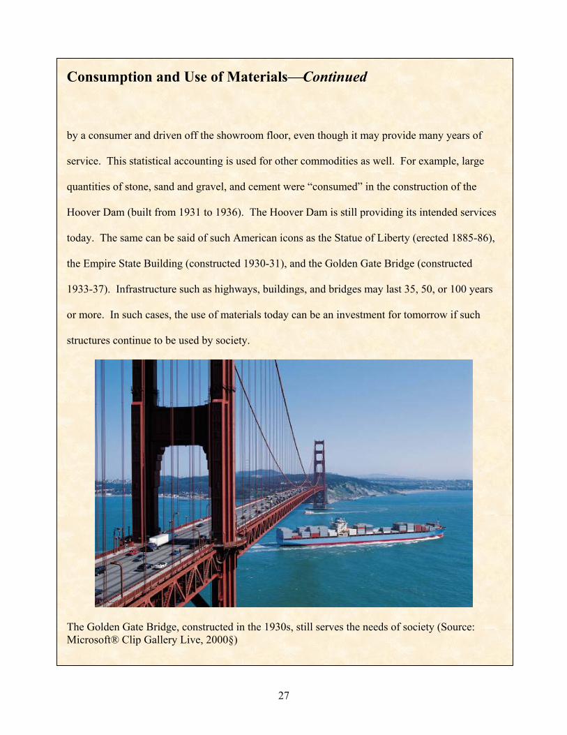
service. This statistical accounting is used for other commodities as well. For example, large
quantities of stone, sand and gravel, and cement were “consumed” in the construction of the
Hoover Dam (built from 1931 to 1936). The Hoover Dam is still providing its intended services
today. The same can be said of such American icons as the Statue of Liberty (erected 1885-86),
the Empire State Building (constructed 1930-31), and the Golden Gate Bridge (constructed
1933-37). Infrastructure such as highways, buildings, and bridges may last 35, 50, or 100 years
or more. In such cases, the use of materials today can be an investment for tomorrow if such
structures continue to be used by society.
The Golden Gate Bridge, constructed in the 1930s, still serves the needs of society (Source: Microsoft® Clip Gallery Live, 2000§)
27

Resources and reserves
How is it possible to use nonrenewable resources without running out in the future? How is it
that nonrenewable resources are still plentiful and in many cases even more available than in the
past as shown by the falling trend in mineral material prices? Except for a few substances,
notably crude oil and natural gas, which are discretely different from the rock masses that
contain them, the quantities of mineral materials in even the upper few miles of the earth’s crust
approach near inexhaustible accounts by current projections. A single cubic mile of average
crustal rock contains a billion tons of aluminum, over 500 million tons of iron, 1 million tons of
zinc, and 600 thousand tons of copper (Brooks, 1973, p. 4).
In 1973, Brooks questioned why did the perception persist that mineral materials are in short
supply with so much material in existence? Much of the confusion comes from different
interpretations of the terms used to describe the amount of material available and the factors that
cause mineral materials to move from one classification to another. Terms such as resources,
reserve base, and reserves are frequently used among experts in this field when discussing the
amount of mineral materials available for extraction. These terms can lead to confusion when
interpreting the actual amount of material left in the ground to be extracted. As stated by
Zwartendyk (1981), “Immense – and immensely misconstruable – figures for mineral resources
fail to impart a clear picture of mineral-resource adequacy and long-term mineral supply. Such
figures are almost routinely mistaken for amounts that will be available at acceptable prices
when and where needed, as if the world were economically frictionless”. Detailed discussions of
28
resource, reserve base and reserves can be found in the sidebar “Resource, Reserve Base, and
Reserve Definitions.”
Resource, Reserve Base, and Reserve Definitions
Through the years, geologists, mining engineers, and others operating in the minerals field have
used various terms to describe and classify mineral resources, which are defined herein include
energy materials. Some of these terms have gained wide use and acceptance, although they are
not always used with precisely the same meaning. The U.S. Geological Survey and the former
U.S. Bureau of Mines developed a common classification and nomenclature system. The most
recent work was published in 1980 as U.S. Geological Survey Circular 831 – “Principles of a
Resource/Reserve Classification for Minerals” (U.S. Bureau of Mines and U.S. Geological
Survey, 1980) and has been reprinted in the publication “Mineral Commodity Summaries” (U.S.
Geological Survey, 2001a, p. 191).
Long-term public and commercial planning must be based on the probability of discovering new
deposits, on developing economic extraction processes for currently unworkable deposits, and on
knowing which resources are immediately available. Thus, resources must be continuously
reassessed in the light of new geologic knowledge, or progress in science and technology, and of
shifts in economic and political conditions. To best serve these planning needs, identified
resources should be classified from two standpoints: (1) purely geologic or physical/chemical
characteristics – such as grade, quality tonnage, thickness, and depth – of the material in place;
and (2) profitability analyses based on costs of extracting and marketing the material in a given
29
Resource, Reserve Base, and Reserve DefinitionsContinued
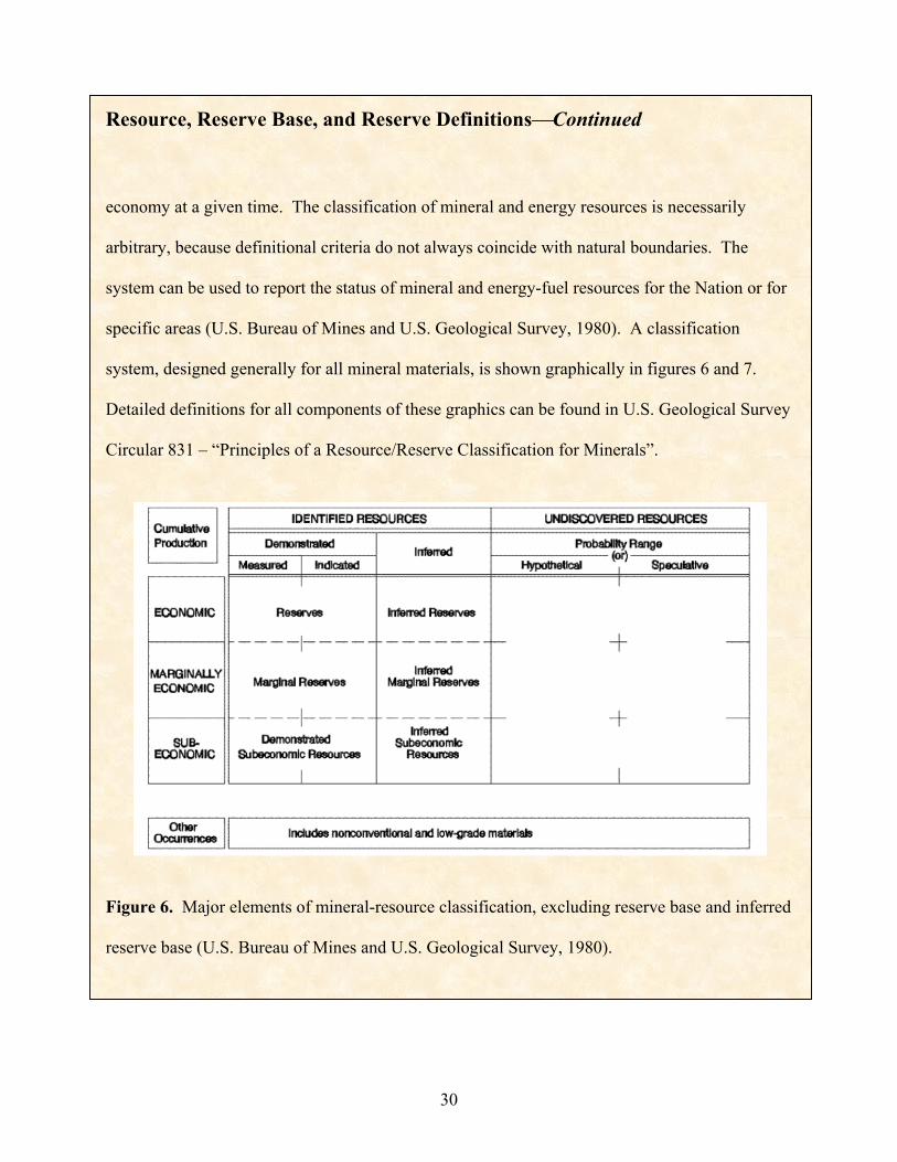
economy at a given time. The classification of mineral and energy resources is necessarily
arbitrary, because definitional criteria do not always coincide with natural boundaries. The
system can be used to report the status of mineral and energy-fuel resources for the Nation or for
specific areas (U.S. Bureau of Mines and U.S. Geological Survey, 1980). A classification
system, designed generally for all mineral materials, is shown graphically in figures 6 and 7.
Detailed definitions for all components of these graphics can be found in U.S. Geological Survey
Circular 831 – “Principles of a Resource/Reserve Classification for Minerals”.
Figure 6. Major elements of mineral-resource classification, excluding reserve base and inferred
reserve base (U.S. Bureau of Mines and U.S. Geological Survey, 1980).
30
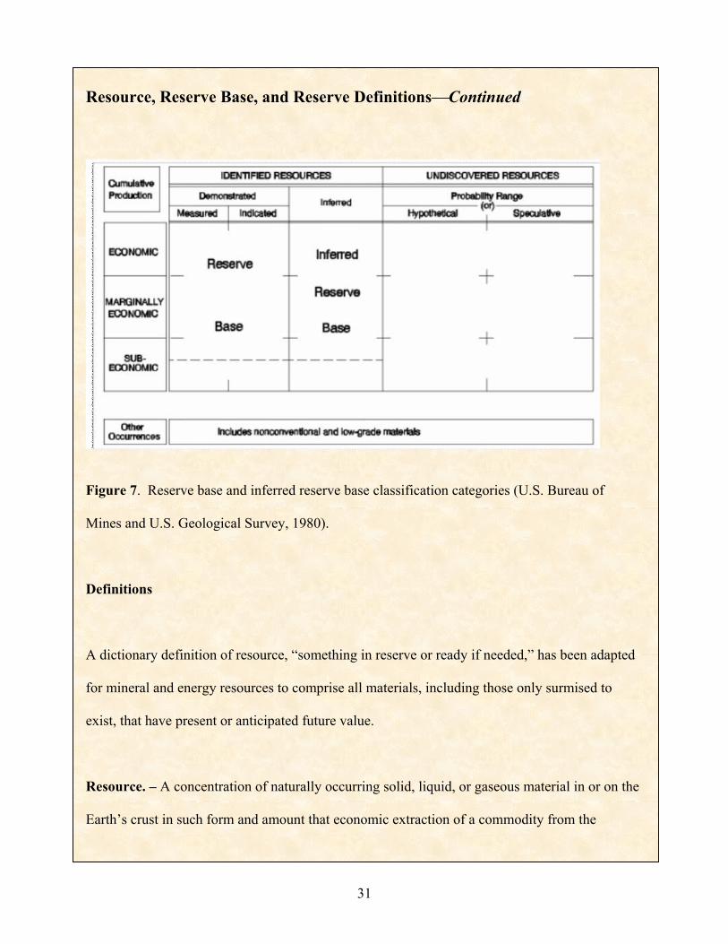
Resource, Reserve Base, and Reserve DefinitionsContinued
Figure 7. Reserve base and inferred reserve base classification categories (U.S. Bureau of
Mines and U.S. Geological Survey, 1980).
Definitions
A dictionary definition of resource, “something in reserve or ready if needed,” has been adapted
for mineral and energy resources to comprise all materials, including those only surmised to
exist, that have present or anticipated future value.
Resource. – A concentration of naturally occurring solid, liquid, or gaseous material in or on the
Earth’s crust in such form and amount that economic extraction of a commodity from the
31
32
Resource, Reserve Base, and Reserve DefinitionsContinued
concentration is currently or potentially feasible (U.S. Bureau of Mines and U.S. Geological
Survey, 1980).
Reserve Base. – That part of an identified resource that meets specified minimum physical and
chemical criteria related to current mining and production practices, including those for grade,
quality, thickness, and depth. The reserve base is the in-place demonstrated (measured plus
indicated) resource from which reserves are estimated. It may encompass those parts of the
resources that have a reasonable potential for becoming economically available within planning
horizons beyond those that assume proven technology, and current economics. The reserve base
includes those resources that are currently economic (reserves), marginally economic (marginal
reserves), and some of those that are currently subeconomic (subeconomic resources). The term
“geologic reserve” has been applied by others generally to the reserve-base category, but it also
may include the inferred-reserve-base category; it is not a part of this classification system (U.S.
Bureau of Mines and U.S. Geological Survey, 1980).
Reserves. – That part of the reserve base that could be economically extracted or produced at the
time of determination. The term “reserves” need not signify that extraction facilities are in place
and operative. Reserves include only recoverable materials; thus, terms such as “extractable
reserves” and “recoverable reserves” are redundant and are not a part of this classification system
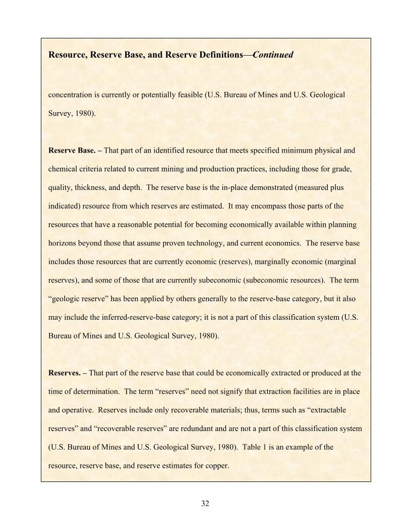
(U.S. Bureau of Mines and U.S. Geological Survey, 1980). Table 1 is an example of the
resource, reserve base, and reserve estimates for copper.
Resource, Reserve Base, and Reserve DefinitionsContinued
Table 1. Copper resource, reserve base, and reserve estimates for the year 2001.
[Data from D.L. Edelstein, 2002, p. 55]
Estimated resources, reserve base, and reserves (Million of metric tons)
Copper Resources United States Discovered 350 Undiscovered 290 Total 640 World Land based 1,600 Deep-sea nodules 700 Total 2,300
Copper Reserve Base United States 90 World 650
Copper Reserves United States 45 World 340
Many descriptions of the supply of mineral materials include only the material that could be
mined at today’s prices and today’s technology – what is properly termed “reserves.” This term
does not include the amount of mineral materials that would be available over the long term with
the development of new technology allowing more ore to be economically mined and with
changing cost and price scenarios. This is the main reason why a common national or world
level analysis of the ‘number of years remaining’ is not valid. As reported by Zwartendyk
(1974), the “life index” of reserves is one such measure, also referred to as the “life expectancy”
of reserves, “reserve life” or “reserves/production ratio.” It is a misleading statistic that is widely
used as a measure of “adequacy” of reserves of a mineral commodity on a national scale. In
33
spite of its serious weaknesses as a statistic, it continues to gain undeserved and unjustified
international respectability. In this analysis, the national or world reserve estimate for a
commodity is divided by the current annual production (or consumption) level to yield the
number of years remaining for production of that particular commodity at current prices.
Because production costs and sales prices change frequently, virtually continuously in some
cases, reserves also change frequently, even though the physical endowment of the earth’s crust
remains constant. As the economics change, mineral material that was once considered a
resource can become a reserve. The amount of mineral material considered a reserve is
influenced by numerous factors such as prices, the development of new technologies, costs to
extract the mineral material, and discoveries of new deposits. Once the mineralized material in a
deposit is considered a reserve (meaning it is economically available), it does not necessarily
exist forever. Product prices can decline and/or costs can rise to levels at which the mineral
deposit becomes uneconomic, whereby reserves of a mine cease to exit economically.
In addition, because delineating reserves requires investment in drilling, stated reserves of a mine
may be approximately the same over many years. Typically, management will desire to have
enough reserves to support production capacity for its planning horizon, for example, 5 to 10
years, and will not delineate more new reserves beyond that planning horizon. In a few States in
America, there is a disincentive to develop additional new reserves as the calculation method for
property taxes includes estimating future production and earnings. As a result, this method of
valuation imposes a tax on the mineral reserves in place. This is a disincentive to exploration
drilling and therefore efficient mine planning, because additions to reserves increase the mine
life, creating greater future earnings and a greater tax liability (Gentry and O’Neil, 1984, p. 182).
34
Thus, as proven reserves are produced; more may be added by additional drilling. For that
reason, it is useful to consider quoted reserves as the current working inventory (Harris, 1985).
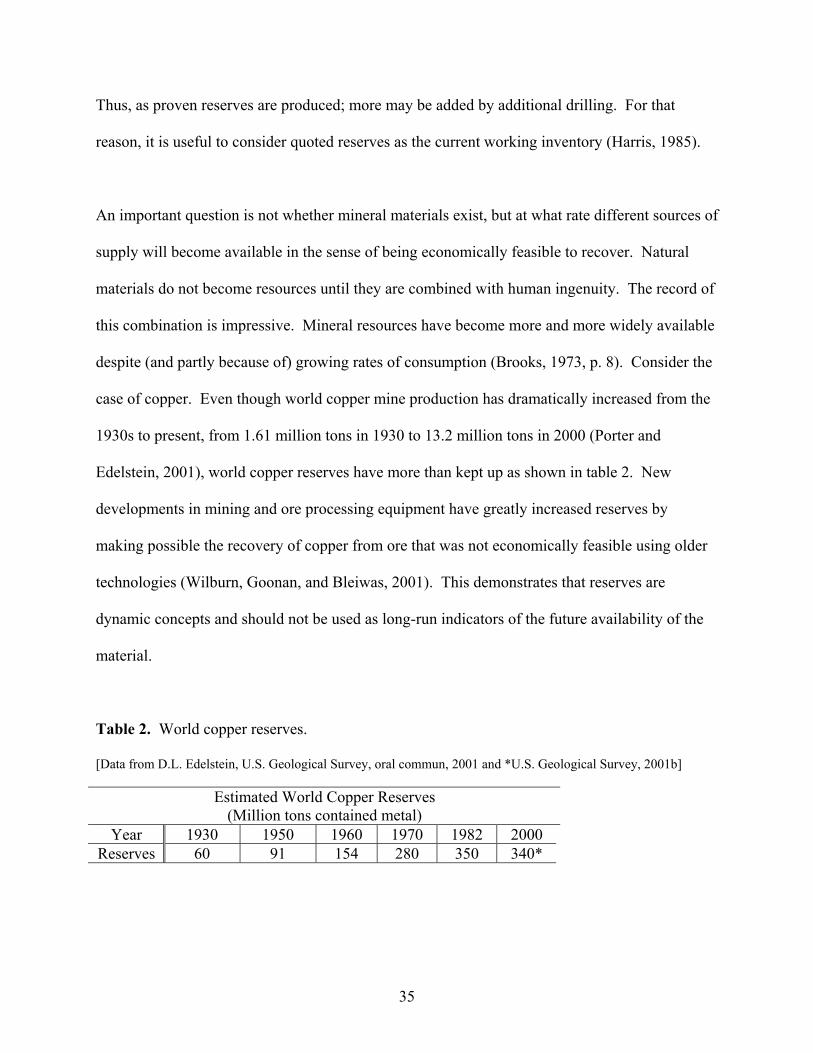
An important question is not whether mineral materials exist, but at what rate different sources of
supply will become available in the sense of being economically feasible to recover. Natural
materials do not become resources until they are combined with human ingenuity. The record of
this combination is impressive. Mineral resources have become more and more widely available
despite (and partly because of) growing rates of consumption (Brooks, 1973, p. 8). Consider the
case of copper. Even though world copper mine production has dramatically increased from the
1930s to present, from 1.61 million tons in 1930 to 13.2 million tons in 2000 (Porter and
Edelstein, 2001), world copper reserves have more than kept up as shown in table 2. New
developments in mining and ore processing equipment have greatly increased reserves by
making possible the recovery of copper from ore that was not economically feasible using older
technologies (Wilburn, Goonan, and Bleiwas, 2001). This demonstrates that reserves are
dynamic concepts and should not be used as long-run indicators of the future availability of the
material.
Table 2. World copper reserves.
[Data from D.L. Edelstein, U.S. Geological Survey, oral commun, 2001 and *U.S. Geological Survey, 2001b]
Estimated World Copper Reserves (Million tons contained metal)
Year 1930 1950 1960 1970 1982 2000 Reserves 60 91 154 280 350 340*
35
Understanding the movement of deposits from the resource to reserve category requires an
explanation of the theoretical relations between supply and demand and a discussion of factors
that can make a deposit economic or noneconomic.
Supply-demand relation theory
In order to try to understand the complex set of economic drivers that influence producer’s
decisions, it is useful as a starting point, to consider the basic economic theory of supply and
demand. Although it is based on several key, and in some cases theoretical assumptions, it
nevertheless allows a number of important decision variables to be identified. If it is assumed
that the market for minerals is perfectly competitive, free from government intervention, and
staffed by rational profit-maximizers, then the scale of mineral production will be determined by
the level of consumer demands and the cost of getting the mineral to them.
What, how, and for whom are the three basic questions related to the supply-demand relation that
every economy must solve. The answers to these questions in a free enterprise economy are
determined primarily by a system of markets and prices. They include:
1. What things will be produced is determined by the votes of consumers – by their
everyday decisions to purchase an item and to not purchase a different item. Ultimately
the money they spend provides the payroll that employees (also consumers) receive in
wages. Thus, the circle is completed (closed).
36
2. How things are produced is determined by the competition between different producers.
In theory, the method that has the lowest cost at any time will displace a more costly
method.
3. For whom things are produced is determined by supply and demand in the markets for
productive services: by interest rates, land rents, profits, and wage rates, all of which go
to determine the income of those who participate in the market.
Therefore, each commodity and each service has a “price.” Workers receive money for what
they sell (their skills), and use this money to buy what they need or want. In this system,
consumers reign and vote with their dollars to get services, or to purchase the things they want.
The dollars of consumers compete against each other for services or commodities, and the people
with the most votes theoretically end up with the most influence on what gets produced and
where those goods go.
If more is wanted of any commodity, the suppliers will receive a large number of new orders.
This increased demand will cause the price of the commodity to rise until more is produced.
Similarly, if more of a commodity is produced than people will buy at the last quoted market
price, the commodity’s price will drop until the excess is absorbed. Since the commodity is now
selling for a lower price, producers will be inclined to produce less. Eventually, the supply and
demand situation will equalize, and that price where this occurs is called the equilibrium price.
There exists at any one time a relation between the market price and the quantity demanded of
that commodity. This relation between price and quantity purchased is shown graphically by the
“demand schedule” or “demand curve.” The demand curve for each individual mineral at any
37
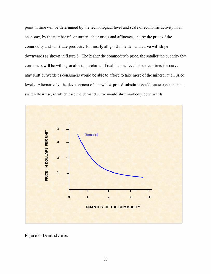
point in time will be determined by the technological level and scale of economic activity in an
economy, by the number of consumers, their tastes and affluence, and by the price of the
commodity and substitute products. For nearly all goods, the demand curve will slope
downwards as shown in figure 8. The higher the commodity’s price, the smaller the quantity that
consumers will be willing or able to purchase. If real income levels rise over time, the curve
may shift outwards as consumers would be able to afford to take more of the mineral at all price
levels. Alternatively, the development of a new low-priced substitute could cause consumers to
switch their use, in which case the demand curve would shift markedly downwards.
QUANTITY OF THE COMMODITY
PRIC
E, IN
DO
LLA
RS
PER
UN
IT
0
Demand
1 2 3 4
4
3
2
1
Figure 8. Demand curve.
38
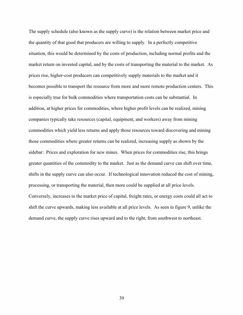
The supply schedule (also known as the supply curve) is the relation between market price and
the quantity of that good that producers are willing to supply. In a perfectly competitive
situation, this would be determined by the costs of production, including normal profits and the
market return on invested capital, and by the costs of transporting the material to the market. As
prices rise, higher-cost producers can competitively supply materials to the market and it
becomes possible to transport the resource from more and more remote production centers. This
is especially true for bulk commodities where transportation costs can be substantial. In
addition, at higher prices for commodities, where higher profit levels can be realized, mining
companies typically take resources (capital, equipment, and workers) away from mining
commodities which yield less returns and apply those resources toward discovering and mining
those commodities where greater returns can be realized, increasing supply as shown by the
sidebar: Prices and exploration for new mines. When prices for commodities rise, this brings
greater quantities of the commodity to the market. Just as the demand curve can shift over time,
shifts in the supply curve can also occur. If technological innovation reduced the cost of mining,
processing, or transporting the material, then more could be supplied at all price levels.
Conversely, increases in the market price of capital, freight rates, or energy costs could all act to
shift the curve upwards, making less available at all price levels. As seen in figure 9, unlike the
demand curve, the supply curve rises upward and to the right, from southwest to northeast.
39
Supply
0 1 2 3 4
4
3
2
1
PRIC
E, IN
DO
LLA
RS
PER
UN
IT
QUANTITY OF THE COMMODITY
Figure 9. Supply curve.
40
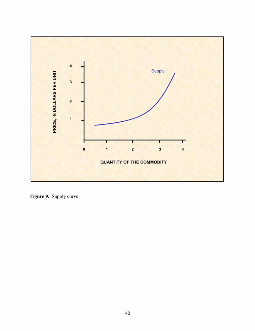
Prices and Exploration for New Mines
From Wilburn, 2001
Prices for some metals in the year 2000 remained near 1999 levels (gold, lead, and silver), and
others inched upward from average 1999 prices (copper and zinc). Significant price increases
for palladium (>64 percent) and nickel (44 percent), and a lower increase for platinum (>3
percent) resulted in some exploration companies reconsidering the mix of commodities being
explored. It appears that during this period of generally low metal prices, the necessity for some
exploration companies to contain costs has led them to shift their exploration focus away from
areas where environmental costs may be significant or exploration more expensive, in spite of
favorable policy climate or geology.
Figure 10 illustrates the distribution of reported mineral exploration budget estimates for 2000 by
commodity grouping. According to the Metals Economics Group (2000) budget estimates, the
principal targets for gold exploration in 2000 were in Latin America, Australia, and the United
States. Gold remained the principal exploration target in 2000, although the exploration budget
for gold in 2000 was 18 percent lower in nominal terms than that budgeted for gold in 1999 and
much lower than the 1997 estimated budget for gold exploration. This decrease probably reflects
the continued depressed gold price, which has declined steadily since 1996 and investor wariness
for funding gold exploration activities while gold remained at a low price level.
41
42
Gold46%
Copper19%
Nickel10%Diamond
10%
Lead and zinc9%
Other mineral commodities
6%
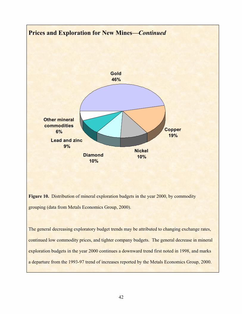
Prices and Exploration for New MinesContinued
Figure 10. Distribution of mineral exploration budgets in the year 2000, by commodity
grouping (data from Metals Economics Group, 2000).
The general decreasing exploratory budget trends may be attributed to changing exchange rates,
continued low commodity prices, and tighter company budgets. The general decrease in mineral
exploration budgets in the year 2000 continues a downward trend first noted in 1998, and marks
a departure from the 1993-97 trend of increases reported by the Metals Economics Group, 2000.
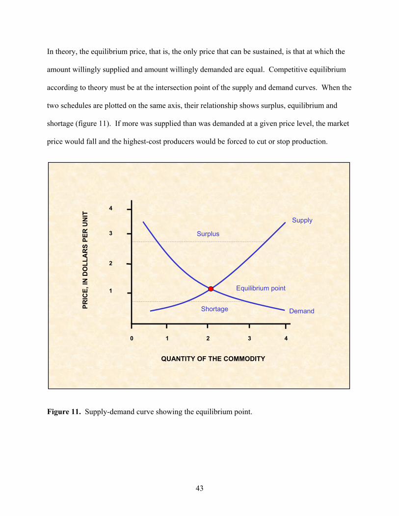
In theory, the equilibrium price, that is, the only price that can be sustained, is that at which the
amount willingly supplied and amount willingly demanded are equal. Competitive equilibrium
according to theory must be at the intersection point of the supply and demand curves. When the
two schedules are plotted on the same axis, their relationship shows surplus, equilibrium and
shortage (figure 11). If more was supplied than was demanded at a given price level, the market
price would fall and the highest-cost producers would be forced to cut or stop production.
Equilibrium point
Demand
Supply
Surplus
Shortage
0 1 2 3 4
4
3
2
1
QUANTITY OF THE COMMODITY
PRIC
E, IN
DO
LLA
RS
PER
UN
IT
Figure 11. Supply-demand curve showing the equilibrium point.
43
As people’s desires and needs change, as technologies used to produce the goods improve, and
as supplies of natural resources and other productive factors change, the marketplace commonly
adjusts by registering changes in the prices and the quantities sold of commodities. The
equilibrium market price and quantity traded of a good will not change as long as both the
demand and supply curve for the item does not shift. However, a shift in one or both of these
curves could lead to the establishment of a new equilibrium position.
The Molybdenum Story – Creation of Markets, Price Changes, and
the Climax Mine
World War I generated the first appreciable uses of molybdenum, when it was substituted for
tungsten in high-speed steels and used as an alloying element in certain steels for military
armament (Blossom, 1985, p. 522). Prior to this time, molybdenum was a laboratory curiosity, a
metallic element that had no use.
As World War I raged in Europe in 1914, British, French, German, and Russian armament
manufacturers competed to buy all available molybdenum (Voynick, 1996, p. 14). Throughout
1914 to 1916, the annual average molybdenum concentrate price, in terms of dollars per
kilogram of molybdenum content, remained at $2.24 as shown by figure 12. This higher price
(from $0.45/kilogram in 1912) triggered commercial molybdenum mining in the United States.
Development of the Climax deposit, the world’s largest, later proved the viability of high-
tonnage extraction of relatively low-grade ore and established the United States as the leading
producer of molybdenum (Blossom, 1985, p 522).
44
0
10
20
30
40
50
60
70
80
1900 1910 1920 1930 1940 1950 1960 1970 1980 1990 2000
YEAR
U.S.
PR
OD
UCTI
ON,
IN T
HO
USA
NDS
OF
MET
RIC
TO
NS
OF
MO
LYB
DEN
UM
C
ON
TEN
T
0
5
10
15
20
25
PRIC
E, IN
DO
LLA
RS
PER
KIL
OG
RA
MM
OLY
BD
ENU
M C
ON
TEN
T
Production Price
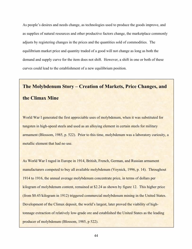
The Molybdenum Story – Creation of Markets, Price Changes, and
the Climax MineContinued
Figure 12. U.S. molybdenum concentrate production and price, 1900 – 2000 (data from Kelly
and Magyar, 2001).
The end of World War I in 1918 signaled changes for the molybdenum market. Output
terminated in 1920 in the United States and most other countries because nonmilitary
consumption of molybdenum was insufficient to support continued production. However,
industrial efforts to develop peacetime applications, primarily as an alloy in steels and cast irons,
were successful, and by the mid-1920s, demand exceeded that of the war years (Blossom, 1985,
p. 522). Operations resumed at the Climax deposit in 1924. By 1930, world output of
45
The Molybdenum Story – Creation of Markets, Price Changes, and
the Climax MineContinued
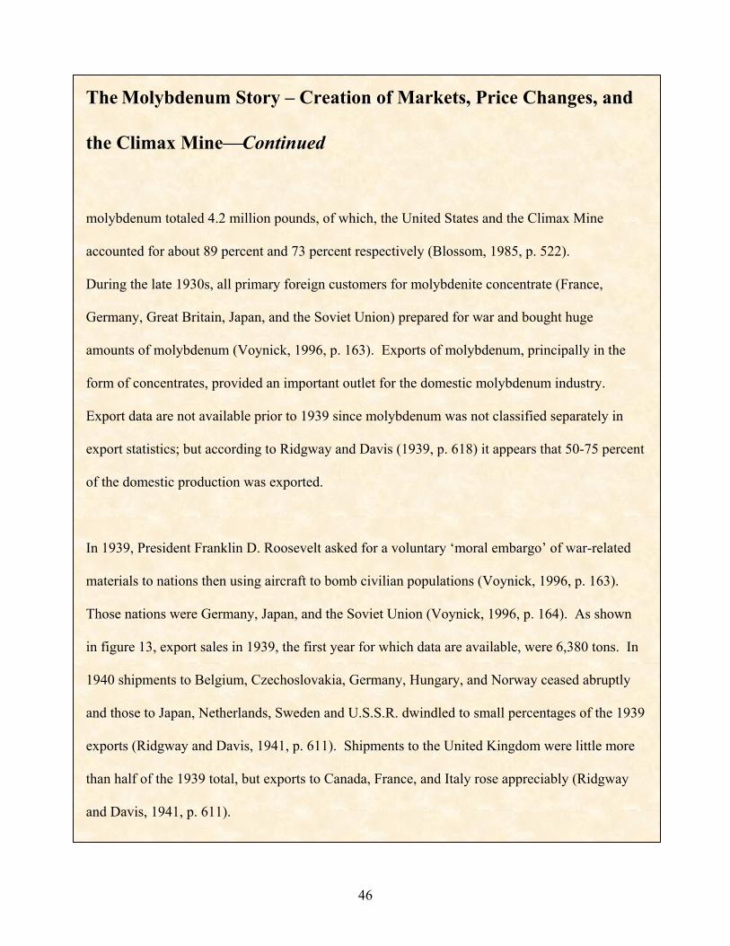
molybdenum totaled 4.2 million pounds, of which, the United States and the Climax Mine
accounted for about 89 percent and 73 percent respectively (Blossom, 1985, p. 522).
During the late 1930s, all primary foreign customers for molybdenite concentrate (France,
Germany, Great Britain, Japan, and the Soviet Union) prepared for war and bought huge
amounts of molybdenum (Voynick, 1996, p. 163). Exports of molybdenum, principally in the
form of concentrates, provided an important outlet for the domestic molybdenum industry.
Export data are not available prior to 1939 since molybdenum was not classified separately in
export statistics; but according to Ridgway and Davis (1939, p. 618) it appears that 50-75 percent
of the domestic production was exported.
In 1939, President Franklin D. Roosevelt asked for a voluntary ‘moral embargo’ of war-related
materials to nations then using aircraft to bomb civilian populations (Voynick, 1996, p. 163).
Those nations were Germany, Japan, and the Soviet Union (Voynick, 1996, p. 164). As shown
in figure 13, export sales in 1939, the first year for which data are available, were 6,380 tons. In
1940 shipments to Belgium, Czechoslovakia, Germany, Hungary, and Norway ceased abruptly
and those to Japan, Netherlands, Sweden and U.S.S.R. dwindled to small percentages of the 1939
exports (Ridgway and Davis, 1941, p. 611). Shipments to the United Kingdom were little more
than half of the 1939 total, but exports to Canada, France, and Italy rose appreciably (Ridgway
and Davis, 1941, p. 611).
46

47
0
10
20
30
40
50
60
70
1910 1920 1930 1940 1950 1960 1970 1980 1990 2000
YEAR
U.S.
EXP
ORT
S AN
D IM
PORT
S O
F M
OLY
BDEN
UM
ORE
S AN
D CO
NCEN
TRAT
ES, I
N TH
OUS
ANDS
OF
MET
RIC
TONS
OF
MO
LYBD
ENUM
CO
NTEN
T
Exports Imports
The Molybdenum Story – Creation of Markets, Price Changes, and
the Climax MineContinued
Figure 13. U.S. exports and imports of molybdenum ores and concentrates, 1918-2000 (data
from Kelly and Magyar, 2001).
In 1941, as in 1940, shipments of molybdenum concentrates from the United States to foreign
countries represented about 19 percent of domestic production, compared to 67 percent in 1939
(Betz and van Siclen, 1943, p. 627). As has been the case for a number of years, the Climax
Molybdenum Co. was the world’s leading producer of molybdenum, and in 1941 it supplied 69
percent of the domestic output (Betz and van Siclen, 1943, p. 627).
The Molybdenum Story – Creation of Markets, Price Changes, and
the Climax MineContinued
In December of 1941, under authority of the Executive War Powers Act, President Roosevelt
placed American industry under the direction of the War Production Board; a quasi-military
agency empowered to control military supply and distribution and to maximize industrial
production (Voynick, 1996, p. 170). Global war made foreign supplies of such alloying metals
as tungsten, chromium, nickel, manganese and vanadium scarce and unreliable, and the ready
availability of tough molybdenum steels was obviously vital to victory (Voynick, 1996, p. 170).
But molybdenum was unique from the standpoint of supply, for no other metal in the world was
so utterly dependent upon a single mine source – the Climax Mine (Voynick, 1996, p. 170). In
January 1942, the War Production Board served notice that it had assigned the Climax Mine the
highest operating priority of any mine in the United States (Voynick, 1996, p. 170). By order of
the War Production Board, the Climax Mine would immediately achieve and maintain maximum
production (Voynick, 1996, p. 170). In an effort to assist in metals production in the United
States, the War Production Board closed all primary gold mines in order to redirect men and
mining materials to the production of iron, coal, and base and alloying metals. In addition, the
War Department released 4,000 experienced miners from military service (Voynick, 1996, p.
173).
Even with American industry working around the clock, a full year passed before molybdenite
ore mined and milled at Climax could be converted, alloyed into steels, manufactured into
armament, and shipped to combat zones (Voynick, 1996, p. 191). When World War II finally
48
The Molybdenum Story – Creation of Markets, Price Changes, and
the Climax MineContinued
ended in August 1945, the Climax Mine produced 5,000 short tons per day as it headed for
uncertainties of a deep postwar depression (Voynick, 1996, p. 192). Over the following years,
Climax, which produced 75 percent of the world’s molybdenum supply, remained the dominant
influence on market price (Voynick, 1996, p. 193). Following the Korean War (1950-1953), the
United States embarked upon an unprecedented, prolonged period of industrial growth and
economic prosperity interrupted only briefly by the recession of 1958 (Voynick, 1996, p. 259).
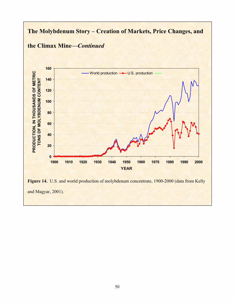
In just 10 years (1960-70), annual world mine production of ores and concentrates doubled as
shown in figure 14. During the 1960s, researchers found new uses in moly-sulfide and moly-
grease lubricants, special corrosion- and abrasion-resistant alloys, and high temperature alloys
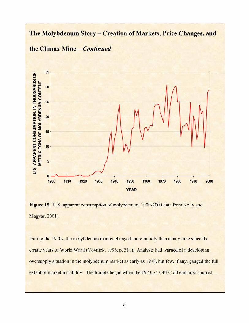
for rocket engine parts for the space program (Voynick, 1996, p. 260). Apparent consumption of
molybdenum in the United States rose throughout the 1960s as shown in figure 15. Throughout
the 1960s prices steadily rose and then rose more rapidly in the mid-1970s. By 1981, the annual
average molybdenum concentrate price had increased to $22.28/kilogram molybdenum content
(Kelly and Magyar, 2001) as shown in figure 12.
49
0
20
40
60
80
100
120
140
160
1900 1910 1920 1930 1940 1950 1960 1970 1980 1990 2000YEAR
PRO
DU
CTI
ON
, IN
TH
OU
SAN
DS
OF
MET
RIC
TO
NS
OF
MO
LYB
DEN
UM
CO
NTE
NT
World production U.S. production
The Molybdenum Story – Creation of Markets, Price Changes, and
the Climax MineContinued
Figure 14. U.S. and world production of molybdenum concentrate, 1900-2000 (data from Kelly
and Magyar, 2001).
50
0
5
10
15
20
25
30
35
1900 1910 1920 1930 1940 1950 1960 1970 1980 1990 2000
YEAR
U.S.
APP
AREN
T CO
NSUM
PTIO
N, IN
THO
USAN
DS O
FM
ETRI
C TO
NS O
F M
OLY
BDEN
UM C
ONT
ENT
The Molybdenum Story – Creation of Markets, Price Changes, and
the Climax MineContinued
Figure 15. U.S. apparent consumption of molybdenum, 1900-2000 data from Kelly and
Magyar, 2001).
During the 1970s, the molybdenum market changed more rapidly than at any time since the
erratic years of World War I (Voynick, 1996, p. 311). Analysts had warned of a developing
oversupply situation in the molybdenum market as early as 1978, but few, if any, gauged the full
extent of market instability. The trouble began when the 1973-74 OPEC oil embargo spurred
51
The Molybdenum Story – Creation of Markets, Price Changes, and
the Climax MineContinued
demand for high-molybdenum oil-field steel, disrupting the projected market growth patterns.
The market tightened further in 1975 when the Federal Government terminated its molybdenum
stockpile disposal sales. Higher prices attracted the attention of competition, namely copper
mining companies, which could recover by-product or co-product molybdenum (Voynick, 1996,
p. 312). As prices offered no prospect of flattening, more molybdenum consumers turned to
alternative alloying metals (Voynick, 1996, p. 315). American mining companies, burdened by
lower-grade ores, escalating environmental restrictions, and high labor costs, was hard-pressed to
compete with higher-grade ores and cheap labor of foreign mines (Voynick, 1996, p. 315).
The depth of the worsening recession became fully apparent in summer of 1981. The
inflationary, soaring oil prices of 1980 began collapsing, killing the drilling boom along with
demand for high-molybdenum oil-field steel. Automotive and general manufacturing slowed
dramatically; U.S. steel companies, operating at half-capacity, laid off thousands of workers.
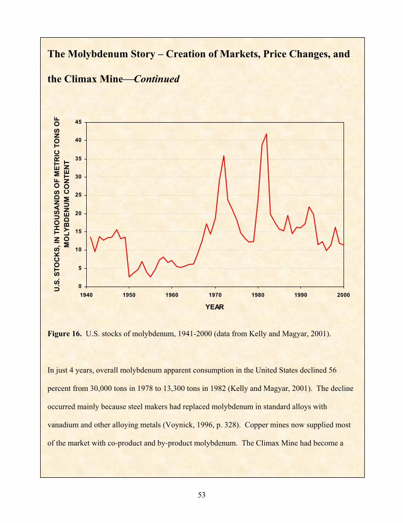
The molybdenum mining industry suddenly faced the worst possible scenario: Burdened with
record stockpiles (figure 16) and a huge overproduction capacity, the molybdenum market began
falling apart (Voynick, 1996, p. 316). In one year, from 1982 to 1983, the average annual
molybdenum concentrate price dropped from $22.80/kilogram to $15.97 per kilogram (Kelly and
Magyar, 2001). At this point in time, the Climax Mine was shut down – layoffs began in
January of 1982 as a result of the continued deterioration of the molybdenum market (Voynick,
1996, p. 319).
52
53
0
5
10
15
20
25
30
35
40
45
1940 1950 1960 1970 1980 1990 2000
YEAR
U.S
. STO
CK
S, IN
TH
OU
SAN
DS
OF
MET
RIC
TO
NS
OF
MO
LYB
DEN
UM
CO
NTE
NT
The Molybdenum Story – Creation of Markets, Price Changes, and
the Climax MineContinued
Figure 16. U.S. stocks of molybdenum, 1941-2000 (data from Kelly and Magyar, 2001).
In just 4 years, overall molybdenum apparent consumption in the United States declined 56
percent from 30,000 tons in 1978 to 13,300 tons in 1982 (Kelly and Magyar, 2001). The decline
occurred mainly because steel makers had replaced molybdenum in standard alloys with
vanadium and other alloying metals (Voynick, 1996, p. 328). Copper mines now supplied most
of the market with co-product and by-product molybdenum. The Climax Mine had become a
The Molybdenum Story – Creation of Markets, Price Changes, and
the Climax MineContinued
‘swing producer’ – they would produce only when warranted by market conditions (Voynick,
1996, p. 328).
The U.S. production of molybdenum reached a peak of 68,400 tons in 1980. The lowest U.S.
production since 1980 was 15,200 tons in 1983. At the end of the 20th century, U.S. production
was trending downward. Molybdenum was being used in many more applications, such as
stainless steel, catalysts and lubricants, with reported consumption averaging over 20,000 tons
per year in the last decade of the century (Blossom, 2002, p. 53.1).
Bartlett Mountain represents the history of the Climax Mine as well as its future (Voynick, 1996,
p. 340). Even after mining 470 million short tons of ore, huge amounts of ore still remain in
place (Voynick, 1996, p. 340). Although underground workings and reserves have been written
off, open pit reserves are estimated at 137 million short tons with an average grade of 0.317
percent molybdenite (Voynick, 1996, p. 340). Contained within those ore reserves are 400
million pounds of elemental molybdenum worth in excess of a billion dollars (Voynick, 1996, p.
340).
Price
Mineral prices are an important driver of mineral supply. In economic theory, the market price is
at the intersection of the supply and demand curves. It is at the equilibrium point where the
54
quantity demanded equals the quantity supplied. Price changes may result from variations in
supply or demand or both. Appendix A contains additional examples of how shifts in demand
and supply can affect equilibrium price and quantity.
When a commodity’s price increases, deposits may become economically viable and allow new
deposits to be developed or previously shutdown operations to reopen. Such activities can
supply more materials to the market. Alternatively, decreasing commodity prices can result in
operations shutting down because they are no longer profitable as discussed in the sidebar:
Prices and Closing Mines.
The demand for, and prices of, many metals are characteristically highly volatile. In economic
theory a demand change would affect price levels, and this would immediately cause the quantity
supplied to change in response. Therefore, shortage and surpluses (and the associated price
fluctuations) should be short-lived features. However, there are four major imperfections within
pure economic theory relative to the operation of the minerals sector that combine to inhibit a
quick market response and act to compound the problems of the cyclical volatility of prices. It
should not be assumed that those minerals markets with relatively stable price trends are less
imperfect and conform more closely to the idealized, perfectly competitive market model; in fact
rather the reverse is true (Rees, 1985, p. 127).
First, since it normally takes at least four years to bring new supply or mineral-based materials
capacity on-stream, shortages can persist resulting in major price rises. Second, once capacity
exists and fixed costs have been incurred, producers are reluctant to curb output as long as some
55
contribution is being made to overhead. Third, price variations are magnified by the nature of
demand for some minerals. The major end-uses for a number of metals are the construction
industry and the production of machinery, commercial vehicles and other intermediate goods, all
of which are more profoundly affected by recession than other sectors of the economy. The
effects of recession will be magnified for the producers of intermediate goods; in their case the
recession will not only be deeper, but also more prolonged, since consumer demand has to pick
up before new orders for plant and machinery are made. The fourth important factor creating
cyclical volatility is the nature of many of the open or auction markets for minerals. In most
cases, these are strictly marginal, that is they deal with only a fraction of total production and
sales (Rees, 1985, p. 127).
Prices and Closing Mines
Although there are additional factors such as environmental, and societal issues that affect the
decision to cease a particular operation, both a commodity’s selling price and the costs to provide
that commodity are integral parts of the final determination. The following examples illustrate
economic impacts upon the mining industry as commodity prices decreased and mining
industries strived to lower their operating costs.
Phelps Dodge Corp., the largest U.S. copper producer, trimmed output by a third and eliminated
1,650 positions to cut costs and streamline operations in 1999. The announcement came against
the backdrop of slumping copper prices, which suffered for the better part of two years due to
decreased demand in the Far East. It also follows a similar announcement recently by Australian
56

Prices and Closing MinesContinued
resource company Broken Hills Proprietary Co. (now BHP Billiton) to shutter its U.S. operations
(Excuria, Inc., 1999§).
The Mesabi Iron Range is located in northern Minnesota. The mining industry in this region was
originally built on the raw ore that lay just beneath the surface. From the 1890s through the
World Wars, the Mesabi Iron Range was the leading producer of iron ore in the United States.
But the mining that fueled the Industrial Revolution and the war effort left the area tapped of its
raw iron reserves by the early 1950s. What saved the Mesabi Iron Range at this time was
taconite, the very hard rock that encases soft-ore deposits and contains 20 to 30 percent iron. In
the 1950s, a complicated process was developed to separate the iron from the rock. Taconite is
blasted out of the ground and loaded onto large trucks and taken to a mill. There, the rock is
processed into a powder (finer than flour) and then passed through a magnetic separator so that
the iron can be removed. The iron is then wetted, mixed with clay and lime, and baked into
marble-sized pellets that are about 80 percent iron. This resulted in a consistent product that
steel makers preferred. This mechanized process, however, required continuous improvements
to maintain a competitive economic edge and over time, these technological upgrades gradually
reduced the number of workers. When taconite was first produced over 30 years ago, the largest
mine in Minnesota produced 14 million tons of pellets a year with 4,200 workers. In 1999, 16
million tons were produced with only 1,500 workers. In recent years, Minnesotans are again
faced with new mine closures as the modernization of the steel industry has led to more efficient
furnaces and decreased use of taconite. The emergence of these processes, cheaper labor, and
57
Prices and Closing MinesContinued
rich iron-ore deposits in other countries are drawing mining companies elsewhere as domestic
steel producers have chosen to relocate their new facilities outside the United States (adapted
from The Christian Science Monitor, 2000, p. 1). These two examples have a common theme.
Economics are major drivers of the mining industry.
Recycling, a significant factor in the supply of many of the metals used in our society, provides
environmental benefits in terms of energy savings, reduced volumes of waste, and reduced
emissions associated with energy savings (Papp, 2002, p. 63.1). For commodities that are
recycled, rising prices tend to bring additional scrap to the market place. In some cases,
significantly higher prices can bring large amounts of material to the market, as is the case for
silver in 1980, see the sidebar: Higher Silver Prices and Increased Recycling.
Higher Silver Prices and Increased Recycling
Following the dramatic rise in the price of gold as a result of rising inflation in the late 1970s, the
average price of silver spiked to an all time historical high in 1980 of almost $43 per troy ounce
(2000 dollars) as shown in figure 17. This final surge was attributed to speculation associated
with the Hunt brothers’ attempt to corner the silver market (Drake, 1981). After topping out in
1980, the price of silver then fell drastically, at one point, to under $5 per troy ounce in 1982.
58
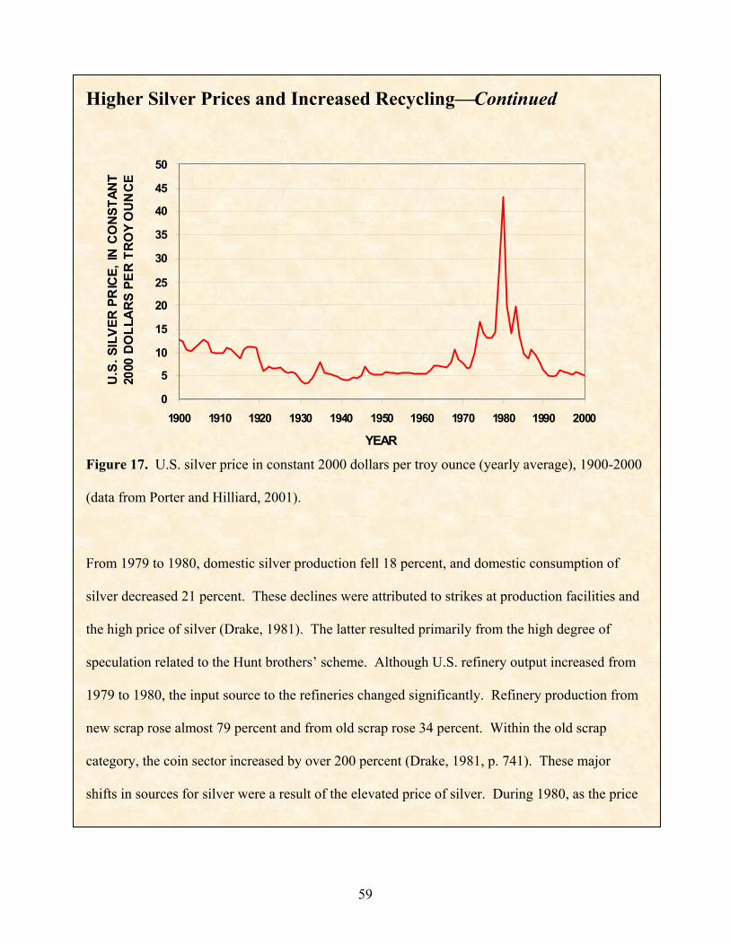
0
5
10
15
20
25
30
35
40
45
50
1900 1910 1920 1930 1940 1950 1960 1970 1980 1990 2000
YEAR
U.S
. SIL
VER
PR
ICE,
IN C
ONS
TAN
T 20
00 D
OLL
ARS
PE
R T
ROY
OU
NC
E
Higher Silver Prices and Increased RecyclingContinued
Figure 17. U.S. silver price in constant 2000 dollars per troy ounce (yearly average), 1900-2000
(data from Porter and Hilliard, 2001).
From 1979 to 1980, domestic silver production fell 18 percent, and domestic consumption of
silver decreased 21 percent. These declines were attributed to strikes at production facilities and
the high price of silver (Drake, 1981). The latter resulted primarily from the high degree of
speculation related to the Hunt brothers’ scheme. Although U.S. refinery output increased from
1979 to 1980, the input source to the refineries changed significantly. Refinery production from
new scrap rose almost 79 percent and from old scrap rose 34 percent. Within the old scrap
category, the coin sector increased by over 200 percent (Drake, 1981, p. 741). These major
shifts in sources for silver were a result of the elevated price of silver. During 1980, as the price
59
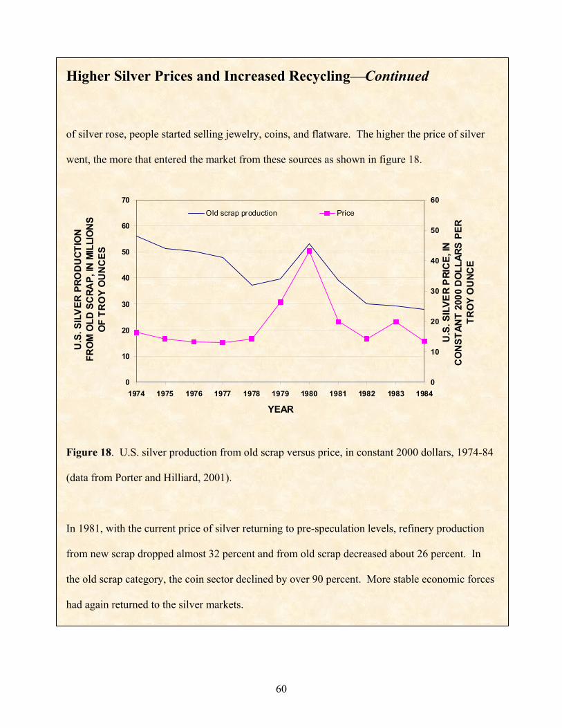
60
0
10
20
30
40
50
60
70
1974 1975 1976 1977 1978 1979 1980 1981 1982 1983 1984
YEAR
U.S
. SIL
VER
PRO
DU
CTIO
N
FRO
M O
LD S
CRA
P, IN
MIL
LIO
NS
OF
TRO
Y O
UN
CES
0
10
20
30
40
50
60
U.S
. SIL
VER
PRI
CE,
IN
CO
NST
ANT
2000
DO
LLAR
S P
ER
TRO
Y O
UNC
E
Old scrap production Price
Higher Silver Prices and Increased RecyclingContinued
of silver rose, people started selling jewelry, coins, and flatware. The higher the price of silver
went, the more that entered the market from these sources as shown in figure 18.
Figure 18. U.S. silver production from old scrap versus price, in constant 2000 dollars, 1974-84
(data from Porter and Hilliard, 2001).
In 1981, with the current price of silver returning to pre-speculation levels, refinery production
from new scrap dropped almost 32 percent and from old scrap decreased about 26 percent. In
the old scrap category, the coin sector declined by over 90 percent. More stable economic forces
had again returned to the silver markets.
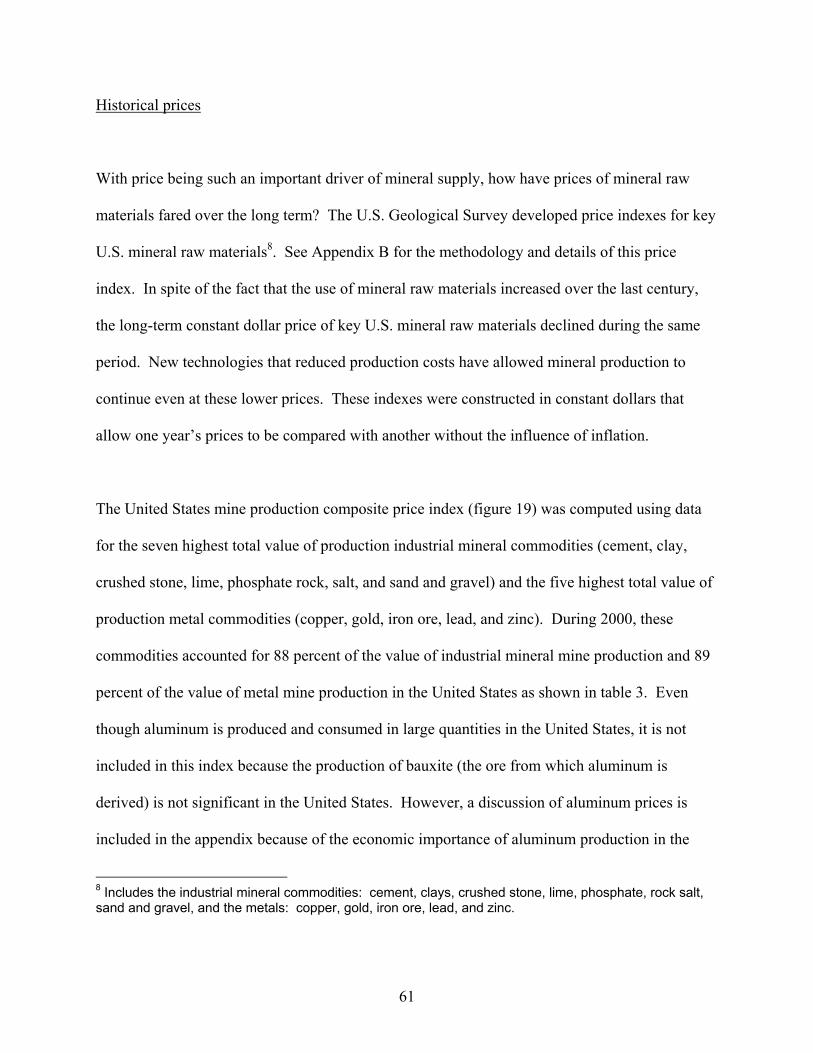
Historical prices
With price being such an important driver of mineral supply, how have prices of mineral raw
materials fared over the long term? The U.S. Geological Survey developed price indexes for key
U.S. mineral raw materials8. See Appendix B for the methodology and details of this price
index. In spite of the fact that the use of mineral raw materials increased over the last century,
the long-term constant dollar price of key U.S. mineral raw materials declined during the same
period. New technologies that reduced production costs have allowed mineral production to
continue even at these lower prices. These indexes were constructed in constant dollars that
allow one year’s prices to be compared with another without the influence of inflation.
The United States mine production composite price index (figure 19) was computed using data
for the seven highest total value of production industrial mineral commodities (cement, clay,
crushed stone, lime, phosphate rock, salt, and sand and gravel) and the five highest total value of
production metal commodities (copper, gold, iron ore, lead, and zinc). During 2000, these
commodities accounted for 88 percent of the value of industrial mineral mine production and 89
percent of the value of metal mine production in the United States as shown in table 3. Even
though aluminum is produced and consumed in large quantities in the United States, it is not
included in this index because the production of bauxite (the ore from which aluminum is
derived) is not significant in the United States. However, a discussion of aluminum prices is
included in the appendix because of the economic importance of aluminum production in the
8 Includes the industrial mineral commodities: cement, clays, crushed stone, lime, phosphate, rock salt, sand and gravel, and the metals: copper, gold, iron ore, lead, and zinc.
61
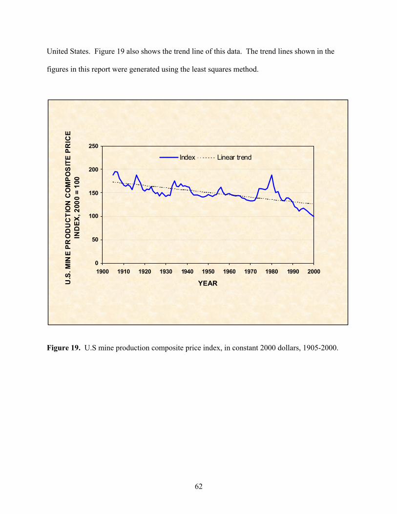
United States. Figure 19 also shows the trend line of this data. The trend lines shown in the
figures in this report were generated using the least squares method.
0
50
100
150
200
250
1900 1910 1920 1930 1940 1950 1960 1970 1980 1990 2000
YEARU.S
. MIN
E PR
OD
UC
TIO
N C
OM
POS
ITE
PR
ICE
IND
EX, 2
000
= 10
0
Index Linear trend
Figure 19. U.S mine production composite price index, in constant 2000 dollars, 1905-2000.
62
Table 3. Value of nonfuel mineral production in the United States in 2000
[Adapted from Smith, 2002]
Material Million dollars Percent Industrial minerals Cement 6,891 23.6 Clays 1,529 5.2 Lime 1,180 4.0 Phosphate rock, marketable1 932 3.2 Salt 1,040 3.6 Sand and gravel 5,946 20.4 Stone, crushed 8,390 28.7 Other industrial minerals 3,292 11.3 Total 29,200 100.0 Metals Copper 2,810 27.5 Gold 3,180 31.2 Iron ore, usable2 1,560 15.3 Lead 439 4.3 Zinc 1,020 10.0 Other metals 1,191 11.7 Total 10,200 100.0 1 The product of additional processing and condensing to the point of salability (S.M. Jasinski, U.S. Geological Survey, oral communication, 2002). 2 Agglomerates, concentrates, direct-shipping ore, and byproduct ore for consumption (U.S. Geological Survey, 2001a, p. 83).
As table 3 shows, the value of industrial minerals production is more than double that of metals.
Therefore, the composite price index is predominantly influenced by the prices of the key
industrial minerals – crushed stone, cement, and sand and gravel. Overall, the trend of the
inflation-adjusted prices shown in the composite price index (figure 19) dropped throughout the
20th century, declining from 185 in 1905 to 100 in the year 2000. This reduction occurred even
though the use of mineral materials in the United States increased during this time frame to meet
the needs of the economy. The decreasing long-term price trend is an indication that adequate
sources of supply exist, competition within the industry is prevalent, and the costs of production
63
have decreased. Detailed analyses of the composite price index in terms of industrial minerals,
metals, and the individual commodities can be found in Appendix B.
Production
According to economic theory, production of mineral commodities occurs to satisfy demand. If
demand for a commodity were nonexistent or decreased due to environmental regulations, prices
would fall and production would decrease, (explained in sidebar: Mercury’s Declining
Production). If production exceeds the amount demanded, a surplus situation is developed and
prices usually decrease to reach a new equilibrium point. In theory, production only occurs to
meet demand. The fact that production of mineral commodities has been able to keep up with or
exceed the demand for minerals is, in part, an indicator that based on the past, scarcity has not
been an issue for mineral resources in general.
Mercury’s Declining Production
In the year 2000, it was estimated that 1,050 tons (64 percent) of the world’s mercury mine
production was to be split evenly between Spain and Kyrgyzstan. The latter represents 86
percent of the former Soviet Union’s production. Other countries that are major producers
include Algeria and China. The trend in world mercury production continues to decline because
of decreased consumption and lower prices.
64
Mercury’s Declining ProductionContinued
Mercury production from mining in the United States has been historically small compared to
other countries. The last operating mercury mine in the United States (McDermitt Mine,
Nevada) closed in 1990. Currently, the only domestic mercury recovered from mining is from
byproduct production from gold and silver mines in several western states, mostly Nevada.
Mercury occurs with gold and silver ores and is usually recovered to avoid contamination of the
environment during gold processing.
Since 1991, recovery of secondary or recycled mercury has surpassed mercury production in the
United States. Because of disposal issues, legal restrictions and potential liability, recovery of
mercury from wastes, in some cases, is more cost effective than disposal. The last time data was
reported, in 1997, mercury recovered by recycling (from discarded and obsolete products such as
batteries, fluorescent lights, dental amalgams, control instruments, and electrolytic wastes) and
U.S. consumption was roughly in balance at slightly under 400 tons. The amount of mercury
recovered from recycling may increase as a result of increasing government regulation.
Historically, mercury had many uses and appeared in many products. Consumption declined as
the toxic nature of this metal became better understood and substitutes were developed mostly as
a result of legislation requiring its elimination from certain products. As an illustration, total
domestic mercury consumption in 1970 was over 2,100 tons, but by 1997 it dropped to under
400 tons. Dissipative mercury uses, such as in paints, have also shown dramatic reductions in
the last decade. Mercury use in paint was about 200 tons in 1985, but was phased out completely
65
Mercury’s Declining ProductionContinued
in the United States by 1992. In addition, mercury use has been essentially eliminated from
household batteries. Since 1989, the largest U.S. consumption of mercury has been in the
production of chlorine and caustic soda. This industry uses approximately one third of the total
domestic consumption. Modern plants have greatly reduced or completely eliminated the need
for mercury and the remaining mercury-cell plants are doing a better job of recycling within their
own systems. In 1997, it was estimated that mercury consumed in this application declined over
50 percent since 1989. (Adapted from Sznopek and Goonan, 2000)
There are four main economic factors which influence where minerals will be produced:
• The existence of an ore body of the appropriate tonnage and grade.
• The location, size, and composition of markets for the mined product.
• The costs of production including the need for infrastructure.
• The costs of transporting the mined material to market.
As markets have changed in their relative importance, so too has the location of the least-cost
mineral production sites. The growth over the last 50 years in the number of mineral producers
throughout the world and the changes in their relative importance in part, at least, reflect the
reduced concentration of mineral consumption. Iron ore mining provides a good illustration of
this. In 1950, the United States dominated world iron ore production, producing 40 percent of
the world total and consuming nearly 44 percent of the world total (Melcher, 1953, p. 615). But
by 2000, the United States produced only approximately 6 percent of the world total and
66
consumed only about 8 percent of total world production (Kirk, 2001, p. 82). Moreover,
although the advanced nations still dominate world steel consumption, industrialization in many
parts of the lesser-developed countries further broadened the range of potential ore markets. As
a consequence, the United States has declined in relative importance as an ore producer and a
wide range of new ore sources have found profitable market outlets. Countries such as Australia,
Brazil, China, India, and Russia, which were either small or non-producers in the 1950s, are
today major supply sources. Australian production is now 158 million tons per year compared
with just over 2 million tons in 1950 (Kirk, 2001, p. 82, and Melcher, 1953, p. 643). Much of
this increase in Australia is attributed to the rapid expansion of the Japanese market.
Favorable Political and Economic Factors Required in Recovering
Mineral Deposits – Congo (Kinshasa)
Markets function within specific economic and political systems. Supply and demand theory
explains how the market system works given certain assumptions. These assumptions include
the ability of producers and consumers to make free, rational, and informed decisions. When
economic and social order breaks down, even a country with a wealth of resources will not be
able to benefit from its resource endowment. The Democratic Republic of the Congo [Congo
(Kinshasa)] is one such example.
In 1985, the state-owned mining companies Generale des Carriers et des Mines du Zaire
(Gecamines) and Societe de Development Industriel et Minier du Zaire produced about 7 percent
67
Favorable Political and Economic Factors Required in Recovering
Mineral Deposits – Congo (Kinshasa)Continued
of global copper mine production, 62 percent of global cobalt mine production, and about 1
percent of world zinc mine output. By 2000, Congo (Kinshasa) produced less than 0.5 percent of
global copper mine production, approximately 20 percent of global cobalt mine production, and
zinc production dropped by over 90 percent. These acute decreases in mineral output from
Congo (Kinshasa) during this 15-year period were a result of a sequence of events that were
unpredictable, but the impacts on their mining industry linger today.
During the early 1990s, the output of copper and cobalt declined precipitously as production was
only 10 percent of capacity. The fall in output was attributable to the collapse of the Kamoto
underground mine in 1990, the flooding of the Dikuluwe and Kova open pit mines in 1991, and
the rioting that damaged Gecamines’ production facilities in 1992. In addition, the redirection of
sales revenue by the Government prevented Gecamines from spending money on maintenance
and reinvestment. After 1995, the fall in copper and cobalt prices exacerbated Gecamines’
difficulties and two civil wars (1996-97 and 1998-2002) discouraged foreign investors from
providing the capital that Gecamines needed to maintain or upgrade its facilities. In early 2002,
decaying national infrastructure and the lack of money for fuel, spare parts, and such process
reagents as sulfuric acid further hobbled Gecamines’ operations. The result of these problems
was that potential foreign investment of more than $2 billion in the minerals sector remained on
hold.
68
Favorable Political and Economic Factors Required in Recovering
Mineral Deposits – Congo (Kinshasa)Continued
The plight of Congo (Kinshasa) demonstrates that having rich mineral resources alone is no
guarantee of the success of a country’s mining sector. Congo (Kinshasa) is a country with
substantial high-grade minerals deposits, but has been unable to utilize this advantage because of
political and economic factors. In the future, Congo (Kinshasa) may be able to revive its
minerals sector with the implementation of a recently signed peace agreement and if the
introduction of a new mining code succeeds in encouraging the flow of capital back into its
mining industries. (Adapted from Coakley and Yager, 2002)
Historical production
Production indexes for raw mineral materials over the last century have been calculated by the
USGS. These indexes incorporate the same mineral commodities that were used to develop the
price indexes.9 Appendix C explains the methodology and details of the production index. The
U.S. composite raw mineral production index is shown in figure 20. This index, similar to the
price index, represents almost 90 percent of the value of domestic production of industrial
minerals and metals. The peaks and troughs of the production index reflect major international
conflicts and other economic events. There was a major downturn during the Great Depression
of the 1930s when raw material demand dried up. A peak was reached during World War II
when many types of materials were needed to construct military equipment. The index bottomed
9 Includes the industrial mineral commodities: cement, clays, lime, phosphate rock, salt, sand and gravel, stone-crushed, and the metals: copper, gold, iron ore, lead, and zinc.
69
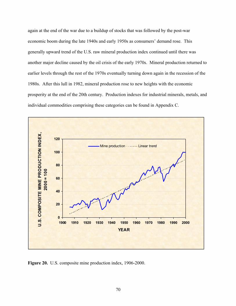
again at the end of the war due to a buildup of stocks that was followed by the post-war
economic boom during the late 1940s and early 1950s as consumers’ demand rose. This
generally upward trend of the U.S. raw mineral production index continued until there was
another major decline caused by the oil crisis of the early 1970s. Mineral production returned to
earlier levels through the rest of the 1970s eventually turning down again in the recession of the
1980s. After this lull in 1982, mineral production rose to new heights with the economic
prosperity at the end of the 20th century. Production indexes for industrial minerals, metals, and
individual commodities comprising these categories can be found in Appendix C.
0
20
40
60
80
100
120
1900 1910 1920 1930 1940 1950 1960 1970 1980 1990 2000
YEAR
U.S
. CO
MPO
SITE
MIN
E P
RO
DU
CTI
ON
IND
EX,
2000
= 1
00
Mine production Linear trend
Figure 20. U.S. composite mine production index, 1906-2000.
70
The U.S. composite raw mineral production index has an increasing long-term trend, exhibiting
nearly a 3 percent average annual growth rate over its 94-year span. In contrast, during its 95
year history the composite price index exhibited an annual average decline of slightly more than
one half of a percent. How can the production index increase over this time period while the
price index, a major driver of mineral supply decline? Such factors as the development of giant
mining trucks, faster and more efficient conveyor systems, and other technologic advancements,
as well as the discovery of additional large-scale economic deposits led to reduced costs of
production. These lower costs of production, plus an increased global supply contributed to
decreased prices.
Globalization
Throughout the 20th century, the speed of communication has increased and the transportation of
materials has become more cost effective. Production technology has constantly improved, and
accessibility to worldwide labor sources and markets has grown as a result of international free
trade agreements such as the North American Free Trade Agreement. These are some of the
factors that have contributed to the globalization of mineral supply.
Globalization refers to a market system that extends beyond national borders and creates
international competition for all materials. Globalization results in part from technological
advances that have made it easier and quicker to complete international transactions for trade
flows. It means greater access to technology, cheaper imports, and larger export markets and
offers greater opportunities for trade in more and larger markets around the world.
71

Historical imports and exports in the United States
As the United States’ economy continues to grow, imports have expanded, reflecting increasing
U.S. consumption. Figure 21 shows total U.S. imports and exports of all goods. Since the early
1980s, the gap between imports and exports continues to widen as the United States economy
becomes more dependent on and integrated within global markets.
0
200
400
600
800
1,000
1,200
1,400
1971 1975 1979 1983 1987 1991 1995 1999
YEAR
TOTA
L U
.S. I
MPO
RTS
AN
D E
XPO
RTS
, IN
B
ILLI
ON
S O
F C
ON
STA
NT
2000
DO
LLA
RS Exports Imports (cost, insurance, freight)
Figure 21. Total U.S. imports and exports in constant 2000 dollars, 1971-2000 (data from
International Monetary Fund, 2001).
72

Imports to the United States of mineral-based materials originate from all over the world. Figure
22 demonstrates the global nature of mineral-based material imports into the United States. This
figure is the result of several factors of which location of mineral-based materials and extraction
costs are the major factors.
73
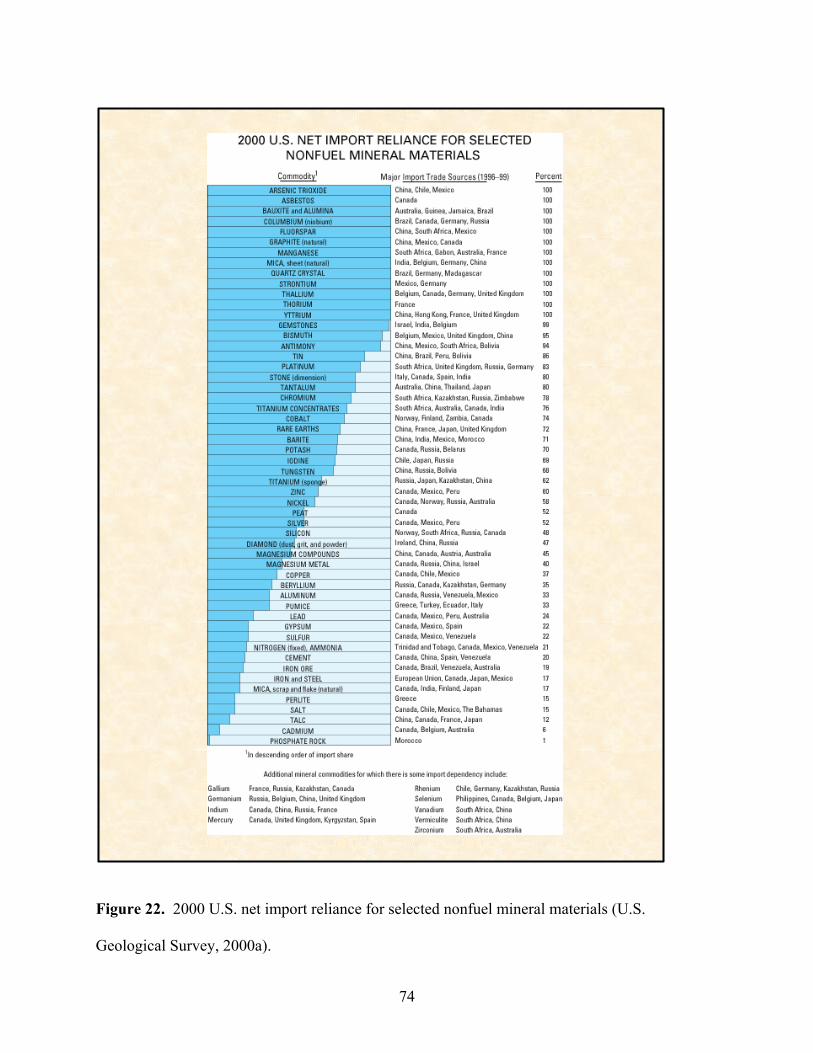
Figure 22. 2000 U.S. net import reliance for selected nonfuel mineral materials (U.S.
Geological Survey, 2000a).
74
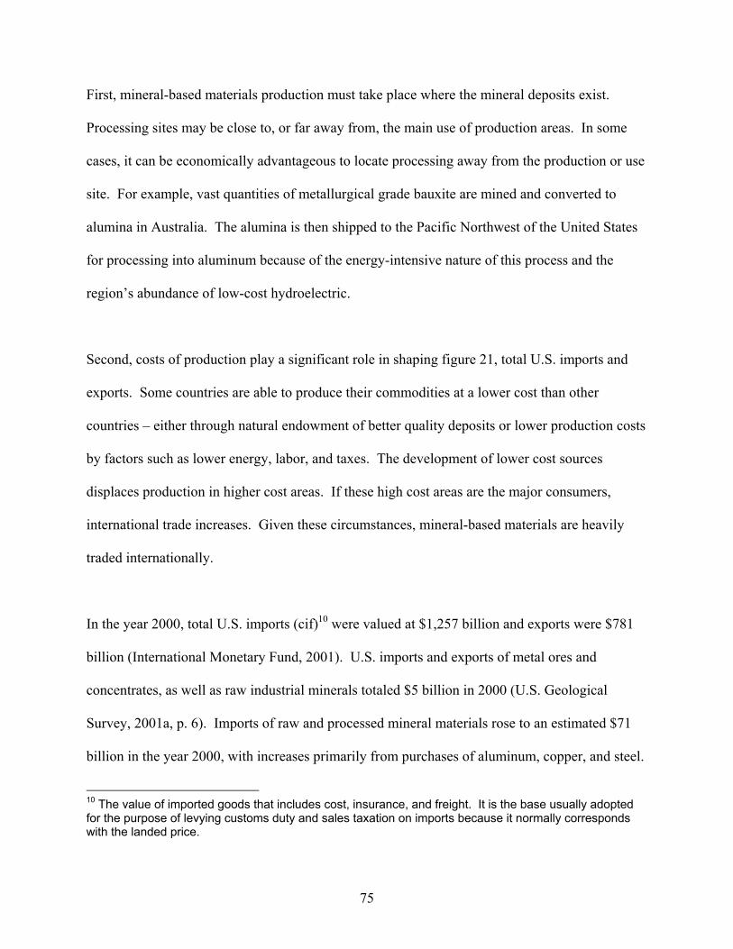
First, mineral-based materials production must take place where the mineral deposits exist.
Processing sites may be close to, or far away from, the main use of production areas. In some
cases, it can be economically advantageous to locate processing away from the production or use
site. For example, vast quantities of metallurgical grade bauxite are mined and converted to
alumina in Australia. The alumina is then shipped to the Pacific Northwest of the United States
for processing into aluminum because of the energy-intensive nature of this process and the
region’s abundance of low-cost hydroelectric.
Second, costs of production play a significant role in shaping figure 21, total U.S. imports and
exports. Some countries are able to produce their commodities at a lower cost than other
countries – either through natural endowment of better quality deposits or lower production costs
by factors such as lower energy, labor, and taxes. The development of lower cost sources
displaces production in higher cost areas. If these high cost areas are the major consumers,
international trade increases. Given these circumstances, mineral-based materials are heavily
traded internationally.
In the year 2000, total U.S. imports (cif)10 were valued at $1,257 billion and exports were $781
billion (International Monetary Fund, 2001). U.S. imports and exports of metal ores and
concentrates, as well as raw industrial minerals totaled $5 billion in 2000 (U.S. Geological
Survey, 2001a, p. 6). Imports of raw and processed mineral materials rose to an estimated $71
billion in the year 2000, with increases primarily from purchases of aluminum, copper, and steel.
10 The value of imported goods that includes cost, insurance, and freight. It is the base usually adopted for the purpose of levying customs duty and sales taxation on imports because it normally corresponds with the landed price.
75
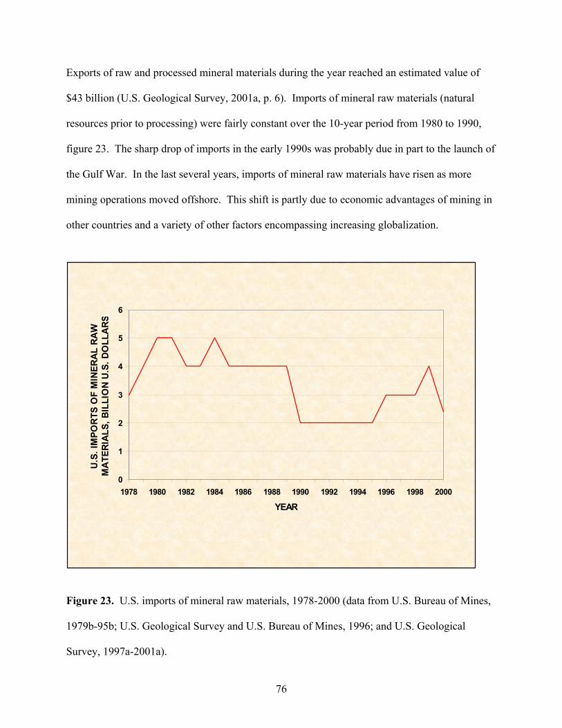
Exports of raw and processed mineral materials during the year reached an estimated value of
$43 billion (U.S. Geological Survey, 2001a, p. 6). Imports of mineral raw materials (natural
resources prior to processing) were fairly constant over the 10-year period from 1980 to 1990,
figure 23. The sharp drop of imports in the early 1990s was probably due in part to the launch of
the Gulf War. In the last several years, imports of mineral raw materials have risen as more
mining operations moved offshore. This shift is partly due to economic advantages of mining in
other countries and a variety of other factors encompassing increasing globalization.
0
1
2
3
4
5
6
1978 1980 1982 1984 1986 1988 1990 1992 1994 1996 1998 2000
YEAR
U.S.
IMPO
RTS
OF
MIN
ERAL
RAW
M
ATER
IALS
, BIL
LIO
N U.
S. D
OLL
ARS
Figure 23. U.S. imports of mineral raw materials, 1978-2000 (data from U.S. Bureau of Mines,
1979b-95b; U.S. Geological Survey and U.S. Bureau of Mines, 1996; and U.S. Geological
Survey, 1997a-2001a).
76
U.S. imports of mineral raw materials as a percent of total U.S. imports are shown in figure 24.
As shown by this figure, U.S. imports of mineral raw materials have remained below 2 percent
of total imports since 1978 and were less than 0.5 percent in 2000.
0.0
0.5
1.0
1.5
2.0
2.5
1978 1980 1982 1984 1986 1988 1990 1992 1994 1996 1998 2000
YEAR
U.S
. IM
POR
TS O
F M
INER
AL
RA
W
MA
TER
IALS
AS
A P
ERC
ENT
OF
TOTA
L U
.S. I
MPO
RTS
Figure 24. U.S. imports of mineral raw materials as percent of total U.S. imports (value based),
1978-2000 (data from International Monetary Fund, 2001; U.S. Bureau of Mines, 1979b-95b;
U.S. Geological Survey and U.S. Bureau of Mines, 1996; and U.S. Geological Survey, 1997a-
2001a).
The declining trend illustrated in figure 24 is an indication that fewer raw materials are being
imported into the United States even though total domestic imports continue to increase (figure
77
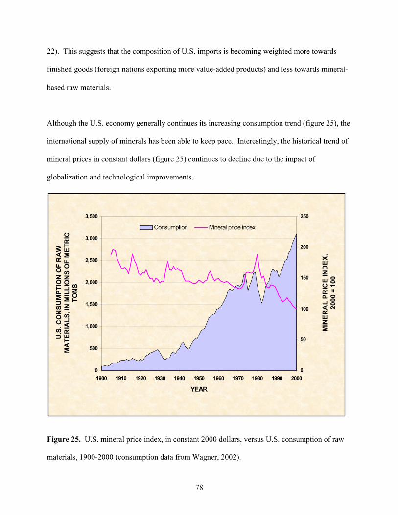
22). This suggests that the composition of U.S. imports is becoming weighted more towards
finished goods (foreign nations exporting more value-added products) and less towards mineral-
based raw materials.
Although the U.S. economy generally continues its increasing consumption trend (figure 25), the
international supply of minerals has been able to keep pace. Interestingly, the historical trend of
mineral prices in constant dollars (figure 25) continues to decline due to the impact of
globalization and technological improvements.
0
500
1,000
1,500
2,000
2,500
3,000
3,500
1900 1910 1920 1930 1940 1950 1960 1970 1980 1990 2000
YEAR
U.S
. CO
NSU
MPT
ION
OF
RA
W
MA
TER
IALS
, IN
MIL
LIO
NS
OF
MET
RIC
TO
NS
0
50
100
150
200
250
MIN
ERA
L PR
ICE
IND
EX,
2000
= 1
00
Consumption Mineral price index
Figure 25. U.S. mineral price index, in constant 2000 dollars, versus U.S. consumption of raw
materials, 1900-2000 (consumption data from Wagner, 2002).
78
Globalization of the Aluminum Industry
Although aluminum was isolated and identified in the early 1800s, a commercial process to
economically recover it was not discovered until the beginning of the 20th century (U.S. Bureau
of Mines, 1985c). The primary source for aluminum is the metallurgical grade of bauxite ore,
which is spread unequally all over the globe. This bauxite ore is treated to obtain aluminum
oxide (alumina), which is further processed to produce aluminum metal.
Aluminum was not widely utilized until WWII when its was incorporated into military aircraft.
Since then, many other uses followed that took advantage of aluminum’s properties of high
strength and lightweight. Automobile components, beverage cans, and foils are just a few of
these applications. Another important advantage of aluminum is that it can be efficiently
recycled requiring far less energy than from the extraction of aluminum from bauxite ore
(Aluminum Association, Inc., 2000§).
Initially, some of the less developed metallurgical-grade bauxite-producing countries operated
their mining operations with no additional processing facilities. If possible, they moved into
higher value processing by producing alumina or aluminum metal. This expansion was primarily
determined by two factors: extensive bauxite deposits and abundant availability of low-cost
energy.
The extraction of aluminum metal from alumina is extremely energy intensive; therefore,
countries that have access to continuous, cheap energy sources (oil, hydroelectric, or natural gas)
79
11 Apparent consumption is defined as: Apparent consumption = production + imports - exports ± (stock
change).
Globalization of the Aluminum IndustryContinued
became prime candidates for aluminum processing. Normally, these conditions did not
coincide; so processing facilities were located away from the mines. As international demand
for aluminum and associated products increased, the development of mining and processing
operations spread worldwide. Paralleling this action, international trade in bauxite, alumina, and
aluminum became routine (U.S. Bureau of Mines, 1985c).
U.S. aluminum trade data and apparent consumption11 are presented in figure 26. Imports and
exports quantities were approximately equal until the early 1990s when they diverged with
imports rising sharply. This trend will probably continue as the domestic aluminum industry
depends more on imports due to higher energy prices and stricter environmental regulations.
The substantial growth of apparent consumption of aluminum in figure 26 reflects the
widespread application of this metal in global industries such as building and construction,
containers and packaging, and transportation.
80
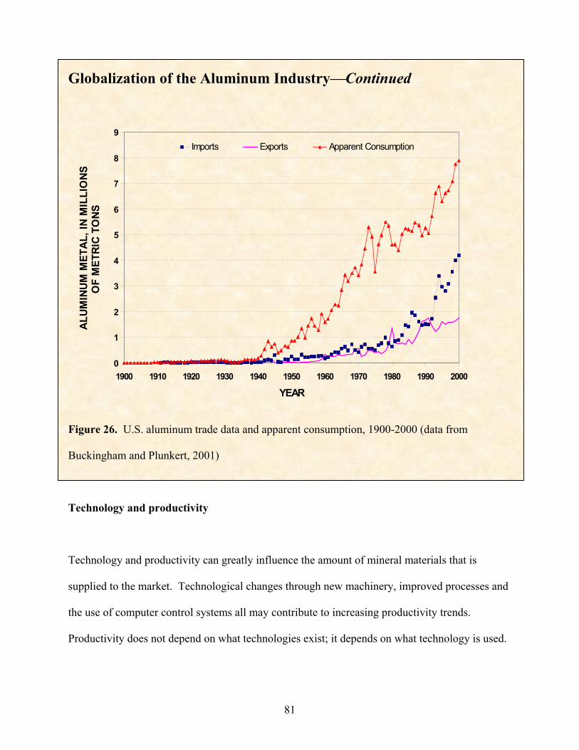
0
1
2
3
4
5
6
7
8
9
1900 1910 1920 1930 1940 1950 1960 1970 1980 1990 2000
YEAR
ALUM
INUM
MET
AL, I
N M
ILLI
ONS
OF
MET
RIC
TONS
Imports Exports Apparent Consumption
Globalization of the Aluminum IndustryContinued
Figure 26. U.S. aluminum trade data and apparent consumption, 1900-2000 (data from
Buckingham and Plunkert, 2001)
Technology and productivity
Technology and productivity can greatly influence the amount of mineral materials that is
supplied to the market. Technological changes through new machinery, improved processes and
the use of computer control systems all may contribute to increasing productivity trends.
Productivity does not depend on what technologies exist; it depends on what technology is used.
81
Improvements in productivity can ultimately lead to economic growth that in turn creates higher
living standards.
The mining industry has seen dramatic improvements in productivity due to advances in
technology. Some technological examples are remote control mining and drilling equipment that
will permit faster extraction and access to previously inaccessible deposits (Thomson, 1999).
This new technology allows additional deposits to be mined, thereby increasing the supply of
materials. Other examples include huge trucks, high volume crushers, high-speed conveyor
belts, and automated control systems that can significantly reduce the costs of producing
minerals. These lower costs result in more deposits being able to be economically mined, in turn
increasing supply.
Productivity is driven by technology and depends to a large extent on production hardware and
software. More information on how technology has changed the mining industry is presented in
Chapter 3 in this series titled “Technological Advancements – A Factor in Increasing Resource
Use” (Wilburn, Goonan, and Bleiwas, 2001).
Labor productivity (LP), which gauges the amount of gross domestic product (GDP) created per
hour of work, is often taken as a measure of how efficient labor is in the economy. The more
GDP each worker can produce, the better off the economy. The concept of increased
productivity relates to a worker’s ability to produce the same output with fewer labor hours,
thereby supplying more materials at a lower per unit cost.
82
Several decades following World War II were often characterized as a “Golden Age” for
industrialized economies (Appelbaum and Schettkat, 1995). During this time frame,
unemployment was low, real incomes increased, and productivity grew. When the era of
computers began in the 1950s, they were used primarily in academic and industrial research to
perform calculations that were impractical or impossible to do manually (Jonscher, 1994).
Technological progress, which implies that a unit of labor can eventually produce more output,
makes a unit of labor more valuable. Given time, this concept theoretically translates into higher
wages and higher standards of living for all.
The United States had the poorest labor productivity record of the seven big industrial economies
during the 1980s, with an average growth of only 1 percent a year, less than half that in Europe
or Japan (The Economist, 1991). Productivity usually goes down in the early stages of a
recession, as most firms are reluctant to lay workers off. As the economy turned upwards at the
end of the 1982, productivity gains were evidence of the impact of American companies’
response to stronger global competition. By trimming jobs as soon as there is an indication of a
slow down, employers attempt to increase productivity. In the last decade, productivity has been
the main driver of economic growth. Productivity growth (manufacturing sector) averaged 4.2
percent per year from 1993 to the end of 1999 (Council of Economic Advisers, 2000).
Productivity increases for all sectors of the United States economy is presented in the Economic
Report of the President, 2002 (Council of Economic Advisers, 2002).
Productivity measures provide important insights into technological changes and the effects of
economic shifts. Important business decisions are made not only on market conditions, but also
83
on the impacts of the various input components that make up the productivity indexes. Although
labor productivity measurements have been traditionally based on output per hour, another
measurement of productivity published by the Bureau of Labor Statistics (BLS) uses a more
complex approach called multifactor productivity (MFP). Multifactor productivity (MFP)
compares changes in output to changes in a composite of inputs used in production – capital,
labor, and intermediate purchases. Capital includes equipment, inventories, land, and structures.
Intermediate purchases are composed of materials, fuels, electricity, and purchased services.12
This expansive input list allows MFP indexes to mirror advances in technology and production
efficiency. Some of the uses for indexes are: economic indicators of technical progress and unit
factor costs; basis for research on the sources of productivity advance; identification of policy
options that can affect the pace of productivity change; aid in understanding trends in output per
hour of all persons; and to provide a more comprehensive productivity measure that incorporates
capital in addition to labor inputs (U.S. Department of Labor, Bureau of Labor Statistics, 2000§).
Historical productivity
Historical labor productivities based upon output per employee hour for two separate sectors of
the mining industries (aluminum and nonmetallic minerals) are shown in figure 27. Each index
reflects the continuous upward productivity trends in the mining industries as technological
improvements came into being. The sidebar: Technology and productivity in the copper
industry contains specific data and more details related to the productivity of the copper industry.
12 For a thorough explanation, refer to the U.S. Department of Labor, Bureau of Labor Statistics, 1997.
84
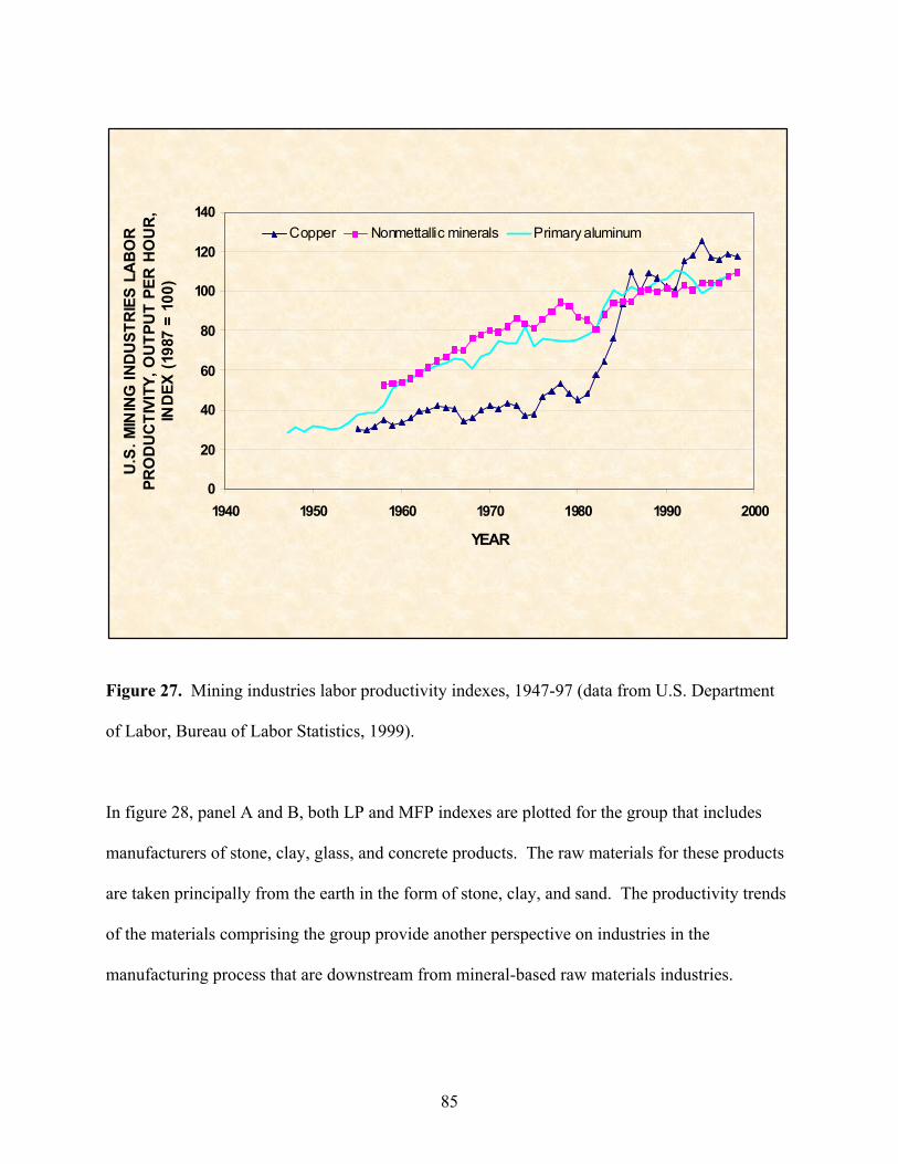
0
20
40
60
80
100
120
140
1940 1950 1960 1970 1980 1990 2000
YEAR
U.S
. MIN
ING
IND
UST
RIE
S L
AB
OR
PR
OD
UC
TIVI
TY, O
UTP
UT
PER
HO
UR
,IN
DEX
(19
87 =
100
)
Copper Nonmettallic minerals Primary aluminum
Figure 27. Mining industries labor productivity indexes, 1947-97 (data from U.S. Department
of Labor, Bureau of Labor Statistics, 1999).
In figure 28, panel A and B, both LP and MFP indexes are plotted for the group that includes
manufacturers of stone, clay, glass, and concrete products. The raw materials for these products
are taken principally from the earth in the form of stone, clay, and sand. The productivity trends
of the materials comprising the group provide another perspective on industries in the
manufacturing process that are downstream from mineral-based raw materials industries.
85
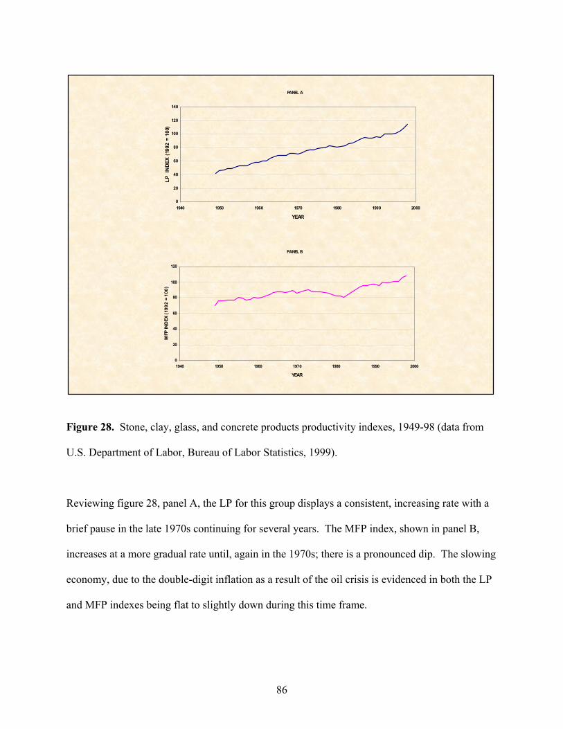
PANEL A
0
20
40
60
80
100
120
140
1940 1950 1960 1970 1980 1990 2000
YEAR
LP I
NDE
X (1
992
= 10
0)
PANEL B
0
20
40
60
80
100
120
1940 1950 1960 1970 1980 1990 2000
YEAR
MFP
INDE
X (1
992
= 10
0)
Figure 28. Stone, clay, glass, and concrete products productivity indexes, 1949-98 (data from
U.S. Department of Labor, Bureau of Labor Statistics, 1999).
Reviewing figure 28, panel A, the LP for this group displays a consistent, increasing rate with a
brief pause in the late 1970s continuing for several years. The MFP index, shown in panel B,
increases at a more gradual rate until, again in the 1970s; there is a pronounced dip. The slowing
economy, due to the double-digit inflation as a result of the oil crisis is evidenced in both the LP
and MFP indexes being flat to slightly down during this time frame.
86
Productivity growth trends have generally increased after WW II with several exceptions. These
stagnant periods were usually associated with recession, for example, 1970s oil crisis, but
technology has continued to provide the means for both higher outputs and shrinking inputs.
Technology and Productivity in the Copper Industry
Reviewing figure 29, the copper industry labor productivity index had a flat to slightly increasing
trend from the 1950s through the 1970s. The 1980s saw a spike up in the index, primarily as a
result of management and labor negotiations that ultimately led to dramatic decreases in labor at
copper mining facilities (Wilburn, Goonan, Bleiwas, 2001, p. 121). In 1970, world copper
reserves were estimated at 280 million tons of contained metal (D.L. Edelstein, USGS, oral
commun., 2000). By 1982, world copper reserves had risen to 350 million tons of contained
metal (D.L. Edelstein, U.S. Geological Survey, oral commun., 2000) partly as a result of the
development of solvent extraction – electrowinning, which could treat lower grade ores. From
1987 to 1997, the labor productivity index resumed its steady increasing trend with the average
annual increase of 1.7 percent (U.S. Department of Labor, Bureau of Labor Statistics, 1999).
87
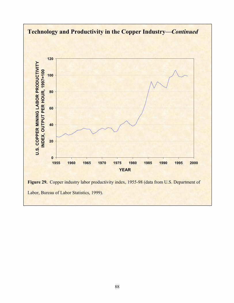
0
20
40
60
80
100
120
1955 1960 1965 1970 1975 1980 1985 1990 1995 2000
YEAR
U.S
. CO
PPER
MIN
ING
LA
BO
R P
RO
DU
CTI
VITY
IN
DEX
, OU
TPU
T PE
R H
OU
R, 1
997=
100
Technology and Productivity in the Copper IndustryContinued
Figure 29. Copper industry labor productivity index, 1955-98 (data from U.S. Department of
Labor, Bureau of Labor Statistics, 1999).
88
Production costs
Production costs have a major impact on the amount of mineral materials that are supplied to the
market. The quantity producers are willing to sell is a result of their production costs and the
market price of the commodity. Producers try to keep their production costs as low as possible
to maintain a competitive place in the marketplace even if prices fall. Under normal
circumstances, if prices fall below costs, operations will tend to shut down, thereby decreasing
the supply of material to the marketplace. As the discussion in Appendix A explains, when this
happens, market forces work to establish a new equilibrium price. If the new equilibrium price is
high enough, closed producers may reopen or new operations may be developed to supply
material to the market.
Table 4 contains cost data for selected mining industries. It is adapted from data published by
the U.S. Census Bureau who compile the data from the economic census that is conducted every
5 years. The Census reports include such statistics as number of establishments, employment,
payroll, value added by mining, cost of supplies used, value of shipments and receipts, capital
expenditures, and other measures for each segment of the mining industry for 1997. This table
(4) reports only selected costs; therefore total costs of mining cannot be derived from this table.
As shown in the table, production costs are made up of operating costs which include for
example, energy, labor, material inputs, overhead, reclamation, and taxes and capital costs such
as acquisition, capital equipment renewal, and exploration.
89
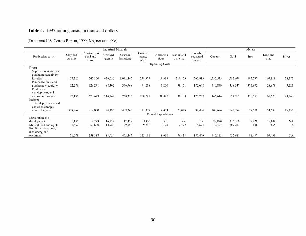
Table 4. 1997 mining costs, in thousand dollars.
[Data from U.S. Census Bureau, 1999; NA, not available]
Industrial Minerals Metals
Production costs Clay and ceramic
Construction sand and
gravel
Crushed granite
Crushed limestone
Crushed stone, other
Dimension stone
Kaolin and ball clay
Potash, soda, and borates
Copper Gold Iron Lead and zinc Silver
Operating Costs
Supplies, material, and purchased machinery installed
157,225
745,100
420,050
1,092,445
278,979
18,989
210,139
300,819
1,333,575
1,597,678
603,797
163,119
28,272 Purchased fuels and purchased electricity
62,278
329,271
88,302
346,968
91,208
8,200
99,151
172,648
410,879
358,337
375,972
28,879
9,221
Production, development, and exploration wages
87,135
679,673
214,162
738,316
208,761
30,827
90,108
177,739
446,646
674,983
330,553
67,623
29,248 Indirect
Total depreciation and depletion charges during the year
318,269
318,060
124,395
408,265
111,027
6,074
73,045
94,404
303,696
643,284
128,570
54,633
16,435 Capital Expenditures
Exploration and development
1,135
12,273
16,132
12,378
11320
531
NA
NA
88,870
216,369
9,420
16,108
NA
Mineral land and rights 1,562 53,600 18,960 29,956 9,998 1,120 2,779 14,694 19,377 207,213 106 NA 6 Buildings, structures, machinery, and equipment
71,078
358,187
183,924
492,447
123,101
9,050
76,433
150,499
440,163
922,668
81,437
93,499
NA
Direct
90
Operating costs include both direct and indirect costs. Direct costs, or variable costs, are those
items such as labor, materials, and supplies, which are consumed directly in the production
process and which are used roughly in direct proportion to the level of production. On the other
hand, indirect costs, or fixed costs, are expenditures that are independent of the level of
production – at least over certain ranges. Examples of fixed costs include such items as office
expenses (buildings, staff), insurance, and property tax. The relatively high level of fixed costs
in mining usually means that the break-even production level for mining facilities is closer to
capacity than for firms with lower fixed costs. This is a major contributing factor in why
operators attempt to run mines at capacity, often employing three-shift, seven-day-per-week
work schedules (Gentry and O’Neil, 1984, p.18).
The production of minerals is a highly capital-intensive activity; the greater the output over
which the capital costs can be spread, the lower the unit production cost. The larger the output at
the site, the greater the use of cost reducing bulk production and transportation technologies. A
small producer, constrained by a limited local market may be forced out of business because of
higher production costs. Larger producers can serve several markets and since they have higher
production volumes, they may be able to take advantage of economies-of-scale and achieve
lower per unit production costs than smaller producers. This has been one factor that has favored
the large multinational companies in relation to small local producers.
The physical characteristics of a particular mineral deposit are only one set among the many
variables that affect the overall production cost at each site. Nevertheless, all other things being
equal, geology and physical geography do play a role in determining which supply sources will
91
be developed first. The size and geometry of the deposit will affect the production level, with
large deposits allowing economies of scale to be achieved. The quality of the mineral and the
possibility of producing co-products or by-products from the same deposit will influence per unit
production costs. Ores of low metal content normally will be more expensive to mine, since a
high proportion of the extracted material will be waste, and even more important, such ores will
involve higher processing costs. The structure of the deposit and its surroundings also affects
production costs. Such factors as whether the deposit can be mined using surface methods, the
thickness of the overburden, and whether de-watering of the mine will be necessary all affect the
costs of production.
Capital costs
In addition to operating costs, mining operations clearly must also consider capital costs. Capital
costs are those expenditures made to acquire or develop capital assets, the benefits from which
will be derived over several years. Capital costs include such items as mining machinery and
equipment, mine development, exploration and property acquisition, and working capital. The
largest share of capital costs is incurred to get the project started, but some capital expenditures
are made yearly throughout the life of the operation (Gentry and O’Neil, 1984, p. 18). The
mining industry is characterized by a high degree of capital intensity because of the large-scale
nature of modern mining activities. In the category of assets per unit of sales, mining ranks near
the top of all industrial sectors (Gentry and O’Neil, 1984, p. 17).
92
Average capital costs for capacity expansions at existing mines are approximately one-half the
cost for nonproducing deposits (Porter and Peterson, 1992). This is because for completely new
mining operations in areas not already established as mining sites, the costs of infrastructure
(hospitals, housing, power plants, recreation facilities, schools, transport and water) are incurred.
These costs can dwarf the capital costs of the mine or processing plant. Significant cost
advantages, therefore, accrue to sites where the mining companies can use existing services or
for those projects that involve the expansion of production at existing mining or processing sites.
If a company has to pay for all the infrastructure, then the mineral deposit would need to be very
large, so that the capital costs could be spread over enough units of output to allow them to be
competitively priced.
Capital costs also affect output levels once production is underway. According to economic
theory, firms will cut output as prices fall and high-cost producers will shut down completely.
However in practice, since the capital costs are fixed and do not vary with output, firms may opt
to maintain output levels as long as the variable costs are covered and at least some contribution
is being made to fixed costs (Rees, 1985, p. 104). Some companies may be able to maintain
loss-making output levels for years, and may find this preferable to abandoning the plant and
losing all the fixed assets. This tends to mean that production levels need not be responsive to a
price fall, supplies continue to exceed demands and prices are driven still lower. This is one of
the factors contributing to metal price volatility as explained on page 43.
93

Strategies for efficient materials usage
New product designs have altered and typically lessened the amount of materials used to
manufacture products, thereby extending the life of mineral deposits. An example is the design
of thin walls for metal beverage containers. This resulted in using less material; therefore, more
aluminum is available for future use. This helps to hold down metal prices, as more costly
deposits do not need to be developed to meet demand. Products are continually reengineered, for
example through substitution of plastic for metal in plumbing and automobile parts, to meet
product requirements while still meeting performance criteria.
Substitution occurs when a different material now satisfies a need that had previously been
satisfied by another material. Substitution can occur in different ways. A new material can
replace the material in a specific product such as the use of aluminum for copper in long distance
electrical transmission lines or plastic replacing steel in automobile bumpers. See the sidebar:
The copper penny. A more subtle form of material substitution occurs when a new product using
different materials replaces the function of an original product, such as cell phones using
airwaves instead of copper wires used by conventional phones. Substitution contributes to
efficient material usage by utilizing more economically available materials. In this way it also
alleviates materials scarcity. If a material becomes relatively scarce, thus more expensive, a less
expensive, more abundant material, available at a lower price, generally replaces it.
Recycling is recovering the material contained in a product at the end of that product’s useful
life. It occurs when the value of the recycled material is sufficient to make recovering profitable.
94
This can occur through natural market forces or when regulations or taxes make recycling
financially attractive. The price received for recycled material governs the amount of material
that is recycled. When materials are recycled they become valuable resources instead of waste.
By supplementing the quantity of material available to the market, recycling conserves virgin
material and makes more material available to the market. Recycling, including composting,
diverted 64 million tons of material away from landfills and incinerators in 1999. In 1999, the
United States recycled 28 percent of its waste, a rate that has almost doubled during the past 15
years (U.S. Environmental Protection Agency, 2002§).
Source reduction means utilizing less material to attain the same economic benefit. This can be
accomplished by changing the design or manufacturing process of these products so less material
is used. Source reduction results in less material entering the disposal stream and when a
product is made using less material then more products can be made with a given quantity of
material. Source reduction has the effect of reducing the physical requirement for materials.
Source reduction saves natural resources, reduces waste, and reduces costs.
95
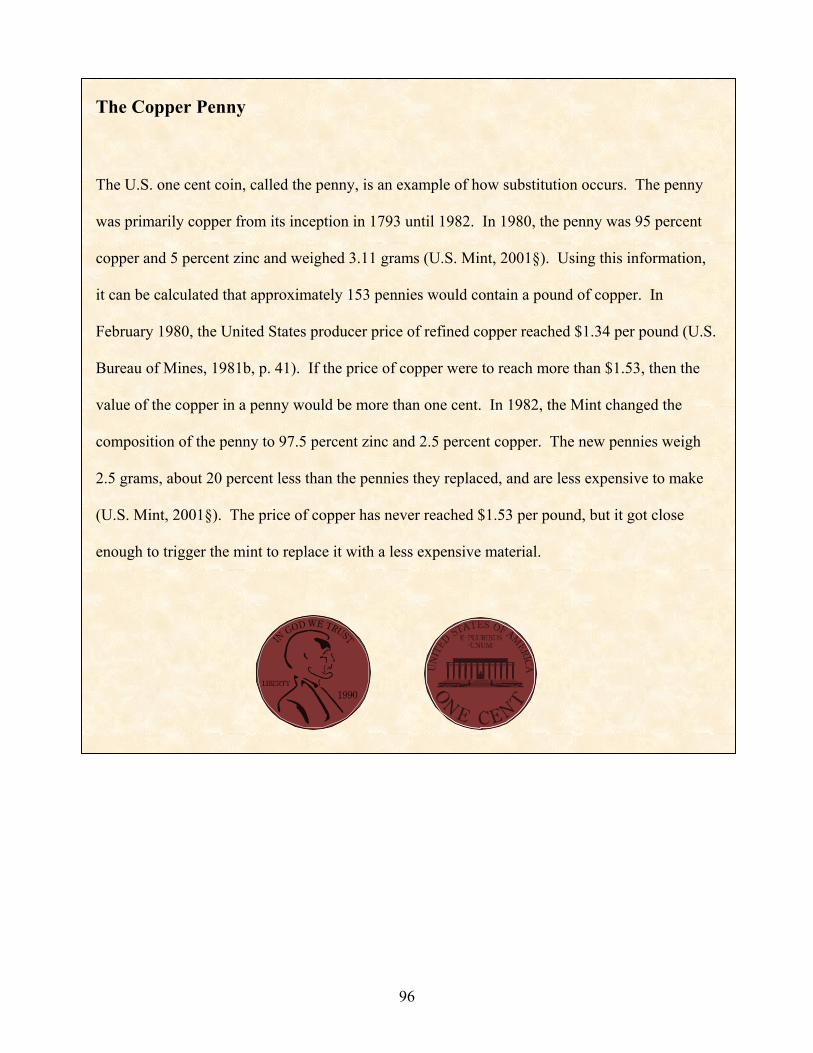
The Copper Penny
The U.S. one cent coin, called the penny, is an example of how substitution occurs. The penny
was primarily copper from its inception in 1793 until 1982. In 1980, the penny was 95 percent
copper and 5 percent zinc and weighed 3.11 grams (U.S. Mint, 2001§). Using this information,
it can be calculated that approximately 153 pennies would contain a pound of copper. In
February 1980, the United States producer price of refined copper reached $1.34 per pound (U.S.
Bureau of Mines, 1981b, p. 41). If the price of copper were to reach more than $1.53, then the
value of the copper in a penny would be more than one cent. In 1982, the Mint changed the
composition of the penny to 97.5 percent zinc and 2.5 percent copper. The new pennies weigh
2.5 grams, about 20 percent less than the pennies they replaced, and are less expensive to make
(U.S. Mint, 2001§). The price of copper has never reached $1.53 per pound, but it got close
enough to trigger the mint to replace it with a less expensive material.
96
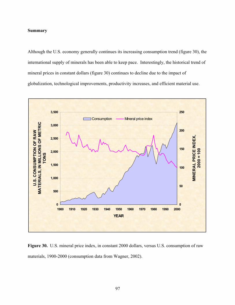
Summary
Although the U.S. economy generally continues its increasing consumption trend (figure 30), the
international supply of minerals has been able to keep pace. Interestingly, the historical trend of
mineral prices in constant dollars (figure 30) continues to decline due to the impact of
globalization, technological improvements, productivity increases, and efficient material use.
0
500
1,000
1,500
2,000
2,500
3,000
3,500
1900 1910 1920 1930 1940 1950 1960 1970 1980 1990 2000
YEAR
U.S
. CO
NSU
MPT
ION
OF
RA
W
MA
TER
IALS
, IN
MIL
LIO
NS
OF
MET
RIC
TO
NS
0
50
100
150
200
250
MIN
ERA
L PR
ICE
IND
EX,
2000
= 1
00
Consumption Mineral price index
Figure 30. U.S. mineral price index, in constant 2000 dollars, versus U.S. consumption of raw
materials, 1900-2000 (consumption data from Wagner, 2002).
97
As shown by the previous discussions, many economic drivers are at work simultaneously to
impact minerals markets and supply. To an economist, a rising long-term price for a commodity
indicates increasing scarcity of supply relative to demand. This is what we should expect with
minerals as depletion progresses. However, in general, mineral prices have historically fallen in
real terms. Therefore, the data show that supply has grown faster than demand. Not all metal
prices have decreased in real terms. Some minerals, such as iron ore and gold, have experienced
price increases, but it cannot be assumed that recent short-term price increases for all mineral
commodities result from increasing long-run scarcity. There are a variety of reasons for
mineral price increases, and these reasons are as much political as they are economic and
geological. Prices for a commodity are, however, relevant. If mineral prices rise, the joint effect
will be to cut demand, increase supply, and encourage recycling. On the demand side, an
immediate tendency will be to turn away from use of expensive minerals and use less expensive
substitutes. At the same time higher prices retard demand, they also increase supply.
Exploration is stimulated and mineral deposits that were formerly too costly to operate may
become working mines. Indeed, there is a strong incentive to find new technologies to work
these deposits economically. If new waste treatment regulations threaten to increase operating
costs, operators may seek ways to reduce the volume of waste, or find more efficient ways to
treat it. Other production problems could be approached in the same way. In addition, new
technologies can result in cost effective mining of unconventional deposits, increasing reserves
of a commodity. Thus the opportunity for technology to augment supplies is extensive. Where
new technology permits an unconventional type of deposit to be mined, the increase could be
very large. For example, the quantities of manganese, copper, and nickel on the deep sea floor
dwarf conventional sources, but recovering them is still too expensive (Brooks, 1973, p. 4).
98
There is strong evidence indicating that vast quantities of mineral resources exist that could be
mined. Further, either as their price goes up or as their cost goes down (which is to say, as
technology of extraction improves), the volume of mineable material could increase significantly
(Brooks, 1973, p. 7). “Since 1800, the trend of prices for the common metals, measured not only
by monetary units but by the cost in human effort, has been almost steadily downward…”
(Hewett, 1929). As shown by the productivity section of this report (figure 28) this trend has
continued into the 21st century.
99
REFERENCES
Appelbaum, Eileen, and Schettkat, Ronald, 1995, Employment and productivity in industrialized economies, in International Labour Review, v. 134, no. 4, July-October, P. 605-624. Betz, Frederick, Jr., and van Siclen, A.P., 1943, Molybdenum, and vanadium, in Minerals Yearbook 1941: U.S. Bureau of Mines, p. 627-641. Blossom, J.W., 2002, Molybdenum, in Metals and Minerals: U.S. Geological Survey Minerals Yearbook 2000, v. I, p. 53.1–53.9. Blossom, J.W., 1985, Molybdenum, in Mineral Facts and Problems, 1985 edition: U.S. Bureau of Mines Bulletin 675, 956 p. Brooks, D.B., 1973, Minerals –An expanding or a dwindling resource?: Department of Energy, Mines and Resources Canada; Mineral Bulletin MR 134, 17 p. Buckingham, D.A., and Plunkert, P.A., 2001, Aluminum statistics, in Historical statistics for mineral commodities in the United States: U.S. Geological Survey Open-File Report 01-006. The Christian Science Monitor, 2000, An uncertain future in iron country—With new mine closure, Minnesotans see their unique way of life slipping away: The Christian Science Monitor, November 21, p. 1. Coakley, G.J., and Yager, Thomas, 2002, Trip report on U.S. Geological Survey visit to mining sectors in Zambia, Democratic Republic of the Congo and Tanzania, January 22 – February2002: U.S. Geological Survey Open-File Report 02-239, 133 p. Council of Economic Advisers, 2000, Economic report of the President: Council of Economic Advisers, Washington, D.C., February, 424 p. Council of Economic Advisers, 2002, Economic report of the President: Council of Economic Advisers, Washington, D.C., February, 441 p. D’Amico, K.J., 1966, Statistical summary, in Metals and Minerals: U.S. Bureau of Mines Minerals Yearbook 1965, v. I, p. 95-134. Drake, H.J., 1981, Silver, in Metals and Minerals: U.S. Geological Survey Minerals Yearbook 1980, v. I, p. 731-745. The Economist (US), 1991, Productivity pickup: The Economist (US), v. 319, no. 7708, May 25, p. 72. Edelstein, D.L., 2002, Copper, in Mineral Commodity Summaries, 2002: U.S. Geological Survey, p. 55.
100
Factor 10 Club, 1995, Carnoules Declaration 1994/1995 of the Factor 10 Club: Wuppertal Institute, Wuppertal, Germany, 6 p. See also, Internet References, Declaration94, 2002, below. Fenton, M.D., 2002, Recycling – Metals – Iron and steel, in Metals and Minerals: U.S. Geological Survey Minerals Yearbook 2000, v. I, p. 63.1-63.16. Gentry, D.W., and O’Neil, T.J., 1984, Mine investment analysis: American Institute of Mining, Metallurgical, and Petroleum Engineers, 502 p. Harris, D.P., 1985, Mineral resource information, supply, and policy analysis, in Economics of the Mineral Industries 4th Edition: American Institute of Mining, Metallurgical, and Petroleum Engineers, 1985, p. 183. Hewett, D.F., 1929, Cycles in metal production, in Transactions of the American Institute of Mining and Metallurgical Engineers, 1929 Yearbook, p. 65-98. International Monetary Fund, 2001, International financial statistics yearbook: Washington, D.C., International Monetary Fund, p. 1031. Jonscher, Charles, 1994, An economic study of the information technology revolution, in Allen, T.J., and Scott-Morton, M.S., Information Technology and the Corporation of the 1990’s, Oxford: Oxford University Press, 1994, pp. 5-42. Kelly, T.D., and Magyar, J.W., 2001, Molybdenum statistics, in Historical statistics for mineral commodities in the United States: U.S. Geological Survey Open-File Report 01-006. Kirk, W.S., 2001, Iron ore, in Mineral Commodity Summaries 2001: U.S. Geological Survey, p. 82-83. Malthus, T.J., 1798, An essay on the principle of population: J. Johnson, London, U.K., 7 p. Matos, G.R., and Wagner, L.A., 1998, Consumption of materials in the United States, 1900-1995: Annual Review of Energy and the Environment 1998, v. 23, p. 107-122. Meadows, D.H., Meadows, D.L., Randers, Jørgen, and Behrens, W.W., III, 1972, The limits to growth: New York, N.Y., Universe Books, 205 p. Melcher, N.B., 1953, Iron ore, in Metals and Minerals: U.S. Bureau of Mines Minerals Yearbook 1950, v.I, p. 613-643. Metals Economics Group, 2000, Metals economics group strategic report 2000: Metals Economics Group, Halifax, Nova Scotia, Canada, 12 p. Papp, J.F., 2002, Recycling – Metals, in Metals and Minerals: U.S. Geological Survey Minerals Yearbook 2000, v. I, p. 63.1-63.16
101
Porter, K.E., and Edelstein, D.L., 2001, Copper statistics, in Historical statistics for mineral commodities in the United States: U.S. Geological Survey Open-File Report 01-006. Porter, K.E., and Hilliard, H.E., 2001, Silver statistics, in Historical statistics for mineral commodities in the United States: U.S. Geological Survey Open-File Report 01-006. Porter, K.E., and Peterson, G.R., 1992, The availability of primary copper in market economy countries –A minerals availability appraisal: U.S. Bureau of Mines Information Circular 9310, 32 p. Rees, Judith, 1985, Natural resources – Allocation, economics, and policy: New York, Methuen & Co. Ltd., 449 p. Ridgway, R.H., and Davis, H.W., 1941, Molybdenum, tungsten and vanadium, in Minerals Yearbook 1941—Review of 1940: U.S. Bureau of Mines Minerals Yearbook 1940, p. 609-628. Ridgway, R.H., and Davis, H.W., 1939, Molybdenum, tungsten and vanadium, in Minerals Yearbook 1939—Review of 1938: U.S. Bureau of Mines Minerals Yearbook 1939, p. 615-631. Smith, S.D., 2002, Statistical summary, in Metals and Minerals: U.S. Geological Survey Minerals Yearbook 2000, v. I, p. 3.1–3.29. Sullivan, D.E., Sznopek, J.L., and Wagner, L.A., 2000, 20th century U.S. mineral prices decline in constant dollars: U.S. Geological Survey Open-File Report 00-389, 9 p. Sznopek, J.L., and Goonan, T.G., 2000, The materials flow of mercury in the economies of the United States and the world: U.S. Geological Survey Circular 1197, 28 p. Thomson, Allison, 1999, Industry output and employment projections to 2008, in Monthly Labor Review, November, p. 33-50. U.S. Bureau of Mines, 1966a-80a and 1982a-95a, Statistical summary, in Metals and Minerals: U.S. Bureau of Mines Minerals Yearbook 1965-77 and 1981-94, v. I. U.S. Bureau of Mines, 1979b-95b, Mineral commodity summaries 1979-95: U.S. Bureau of Mines. U.S. Bureau of Mines, 1985c, Mineral facts and problems, 1985 edition: U.S. Bureau of Mines Bulletin 675, 956 p. U.S. Bureau of Mines and U.S. Geological Survey, 1980, Principles of a resource/reserve classification for minerals: U. S. Geological Survey Circular 831, 5 p. U.S. Census Bureau, 1999, Various reports, in 1997 Economic Census– Mining: U.S. Census Bureau, EC97N-2122, and EC97N-21232.
102
U.S. Census Bureau, 1975, Historical statistics of the United States– Colonial times to 1970: U.S. Census Bureau series E 135, v. I, p. 210-211. U.S. Department of Labor, Bureau of Labor Statistics, 1997, Handbook of methods: U.S. Department of Labor, Bureau of Labor Statistics, April 1997, p. 89-99. U.S. Department of Labor, Bureau of Labor Statistics, 1999, Unit labor costs for selected industries, 1987-97: U.S. Department of Labor, Bureau of Labor Statistics, November 1999. U.S. Geological Survey, 1997a-2001a, Mineral commodity summaries 1997-2001: U.S. Geological Survey. U.S. Geological Survey, 1997b-2001b, Statistical summary, in Metals and Minerals: U.S. Geological Survey Minerals Yearbook 1995-1999, v. I. U.S. Geological Survey and U.S. Bureau of Mines, 1996, Mineral commodity summaries 1996: U.S. Geological Survey and U.S. Bureau of Mines, 195 p. Voynick, S.M., 1996, Climax – The history of Colorado’s climax molybdenum mine: Missoula, Montana, Mountain Press Publishing Company, 364 p. Wagner, L.A., 2002, Materials in the economy—Material flows, scarcity, and the environment: U.S. Geological Survey Circular 1221, 29 p. Wilburn, D.R., 2001, Exploration: Mining Engineering, v. 53, no. 5, May, p. 41-51. Wilburn, D.R., Goonan, T.G., Bleiwas, D.I., 2001, Technological advancement – A factor in increasing resource use: U.S. Geological Survey Open File Report 01-197, 154 p. Zwartendyk, Jan, 1974, The life index of mineral reserves—A statistical mirage: CIM Bulletin, V. 67, no. 750, October, p. 67-70. Zwartendyk, Jan, 1981, Economic issues in mineral resource adequacy and in the long-term supply of minerals: Economic Geology, v. 76, no. 5, August, p. 999-1005. Internet references cited
Aluminum Association, Inc., 2000, Recycling results, accessed October 17, 2000, at URL http://www.aluminum.org/ default2.cfm/4/35. Aluminum Association, Inc., 2001, Americans recycle 2 of 3 aluminum cans, accessed October 19, 2001, at URL http://www.aluminum.org/newsa.cfm?pressid=108.
103
Declaration94, 2002, 1994 declaration of the Factor 10 Club, accessed July 19, 2002, at URL http://www.techfak.uni-bielefeld.de/~walter/f10/declaration94.html. Excuria, Inc., 1999, Phelps shuttering plants – No. 1 copper producer cutting 1,650 jobs as demand, prices decline, June 30, 1999, accessed June 28, 2001, at URL http://www.excuria.com/bizop.asp?IID=11714&SRC=altavista. Steel Recycling Institute, 2001, Fact sheet—A few facts about steel – North America’s #1 recycled material, accessed October 19, 2001 at URL http://www.recycle-steel.org/fact/main.html. U.S. Department of Labor, Bureau of Labor Statistics, 2000, Multifactor productivity overview, accessed November 6, 2000, at URL http://stats.bls.gov/mprover.htm. U.S. Department of Labor, Bureau of Labor Statistics, 2001, Consumer price indexes, accessed December 18, 2001, at URL ftp://ftp.bls.gov/pub/special.requests/cpi/cpiai.txt. U.S. Environmental Protection Agency, Office of Solid Waste, 2002, Recycling, accessed July 16, 2002, at URL http://www.epa.gov/epaoswer/non-hw/muncpl/recycle.htm. U.S. Mint, 2001, The composition of the cent, accessed March 5, 2001, at URL http://www.usmint.gov/faqs/circulating_coins/index.cfm. Photo credits Brøderbund Software, Inc., 1997, ClickArt® 300,000—Premiere image pak: Brøderbund Software, Inc. Microsoft®, Inc., 2000, Microsoft® Clip Gallery Live, accessed August 2, 2000, at URL http://cgl.microsoft.com/clipgallerylive/default.asp.
104
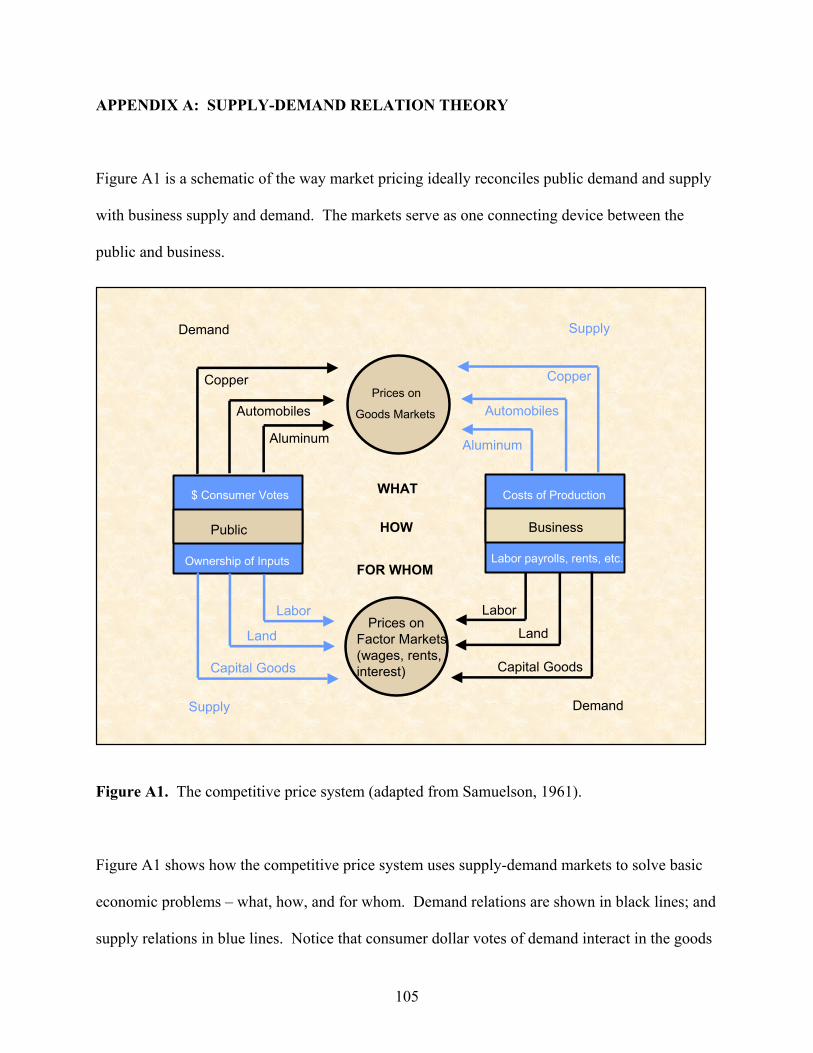
APPENDIX A: SUPPLY-DEMAND RELATION THEORY
Figure A1 is a schematic of the way market pricing ideally reconciles public demand and supply
with business supply and demand. The markets serve as one connecting device between the
public and business.
Supply
Capital Goods
Land
Labor
Aluminum
Automobiles
Copper
Supply
$ Consumer Votes
Ownership of Inputs
Costs of Production
Labor payrolls, rents, etc.
Labor
Land
Capital Goods
Demand
Demand
Copper
Automobiles
Aluminum
Prices on
Goods Markets
Prices on Factor Markets (wages, rents, interest)
WHAT
HOW
FOR WHOM
Public Business
Figure A1. The competitive price system (adapted from Samuelson, 1961).
Figure A1 shows how the competitive price system uses supply-demand markets to solve basic
economic problems – what, how, and for whom. Demand relations are shown in black lines; and
supply relations in blue lines. Notice that consumer dollar votes of demand interact in the goods
105
markets (upper half of schematic) with business-cost supply decisions, thus helping determine
“What” is produced. Also shown is how business demand for inputs or productive factors meets
the public’s supply of labor and other inputs in the factor markets (lower half of schematic) to
help determine wage, rent, and interest income – that is, “For Whom” goods are produced.
Business competition to buy factor inputs and sell goods most cheaply determines “How” goods
are to be produced. It is important to understand that all parts of this diagram interact with one
another.
It is also important to remember that this schematic represents economic theory in a perfect
market and does not take externalities into account. Externalities (or external costs and benefits)
are simply the uncompensated side effects of any economic or social activity that are not
considered by individuals when making private decisions. The word ‘uncompensated’ is
important as it serves to exclude all the external costs and benefits that arise in the course of
normal market transactions. Externalities occur when the by-products of an activity result in
costs or benefits to other people, which go uncompensated by exchange of money or goods.
Whenever producers or consumers make usage decisions on the basis of their own private costs
and benefits and are allowed to neglect the external effects of their actions, the usage patterns are
likely to deviate markedly from those that are socially optimal or desirable (Rees, 1985, p. 244).
This next section will explain how supply and demand work together in a competitive market to
reach an equilibrium point for a commodity. Additional examples of the workings of supply and
demand are found in the main text of this report.
106
Supply and demand schedules
As people’s desires and needs change, as technologies used to produce the goods change, as
supplies of natural resources and other productive factors change, the marketplace registers
changes in the prices and the quantities sold of commodities. For example, assuming figure A2
represents the supply-demand situation for copper where markets with large numbers of buyers
and sellers are free from government interference or monopolization, theoretically, an
equilibrium price will be generated. It is important to note that for illustrative purposes, straight
lines are used to represent the supply and demand curves. For more detail on the supply-demand
relation see Miller, 1998.
107
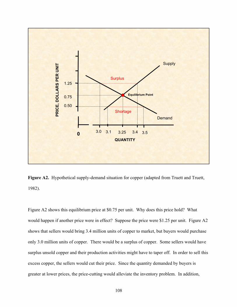
QUANTITY
PRIC
E, D
OLL
ARS
PER
UN
IT
0
Demand
Supply
0.75
0.50
1.25
Equilibrium Point
3.25 3.53.0 3.43.1
Surplus
Shortage
Figure A2. Hypothetical supply-demand situation for copper (adapted from Truett and Truett,
1982).
Figure A2 shows this equilibrium price at $0.75 per unit. Why does this price hold? What
would happen if another price were in effect? Suppose the price were $1.25 per unit. Figure A2
shows that sellers would bring 3.4 million units of copper to market, but buyers would purchase
only 3.0 million units of copper. There would be a surplus of copper. Some sellers would have
surplus unsold copper and their production activities might have to taper off. In order to sell this
excess copper, the sellers would cut their price. Since the quantity demanded by buyers is
greater at lower prices, the price-cutting would alleviate the inventory problem. In addition,
108
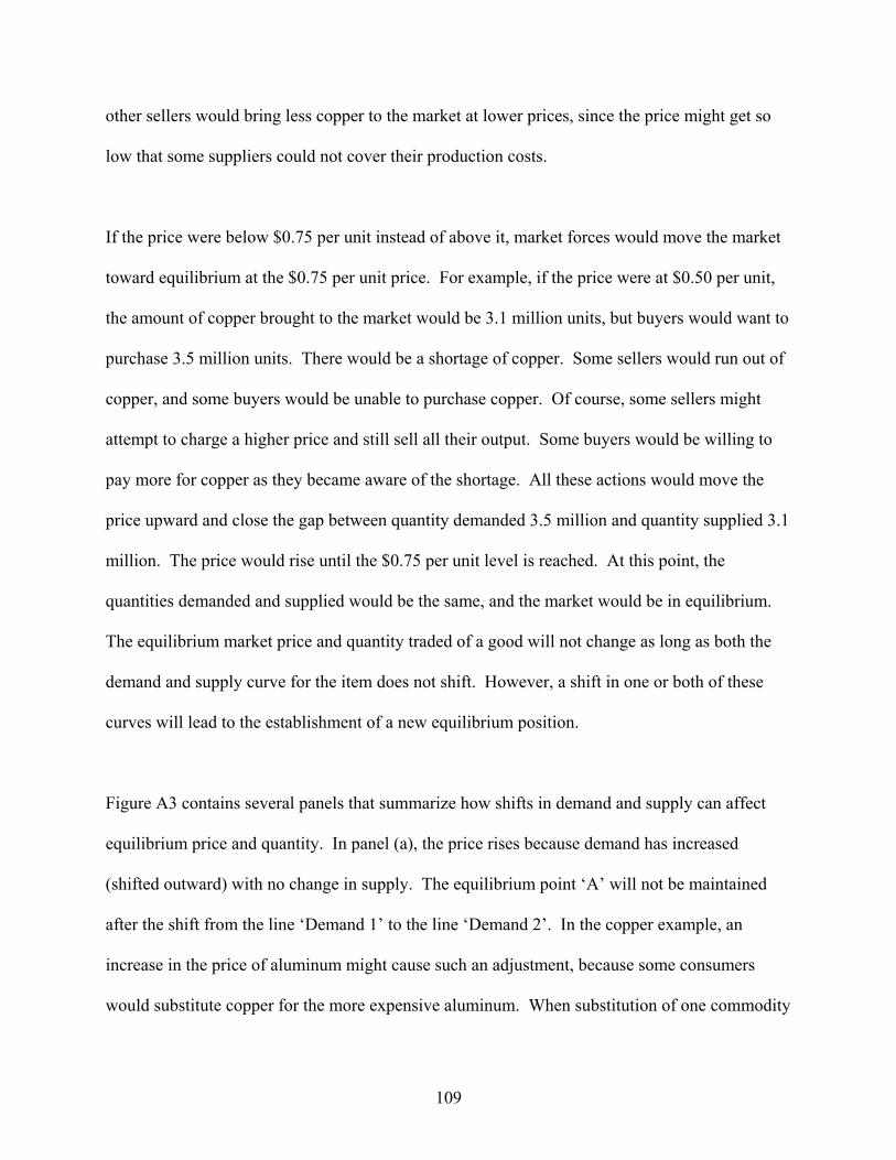
other sellers would bring less copper to the market at lower prices, since the price might get so
low that some suppliers could not cover their production costs.
If the price were below $0.75 per unit instead of above it, market forces would move the market
toward equilibrium at the $0.75 per unit price. For example, if the price were at $0.50 per unit,
the amount of copper brought to the market would be 3.1 million units, but buyers would want to
purchase 3.5 million units. There would be a shortage of copper. Some sellers would run out of
copper, and some buyers would be unable to purchase copper. Of course, some sellers might
attempt to charge a higher price and still sell all their output. Some buyers would be willing to
pay more for copper as they became aware of the shortage. All these actions would move the
price upward and close the gap between quantity demanded 3.5 million and quantity supplied 3.1
million. The price would rise until the $0.75 per unit level is reached. At this point, the
quantities demanded and supplied would be the same, and the market would be in equilibrium.
The equilibrium market price and quantity traded of a good will not change as long as both the
demand and supply curve for the item does not shift. However, a shift in one or both of these
curves will lead to the establishment of a new equilibrium position.
Figure A3 contains several panels that summarize how shifts in demand and supply can affect
equilibrium price and quantity. In panel (a), the price rises because demand has increased
(shifted outward) with no change in supply. The equilibrium point ‘A’ will not be maintained
after the shift from the line ‘Demand 1’ to the line ‘Demand 2’. In the copper example, an
increase in the price of aluminum might cause such an adjustment, because some consumers
would substitute copper for the more expensive aluminum. When substitution of one commodity
109
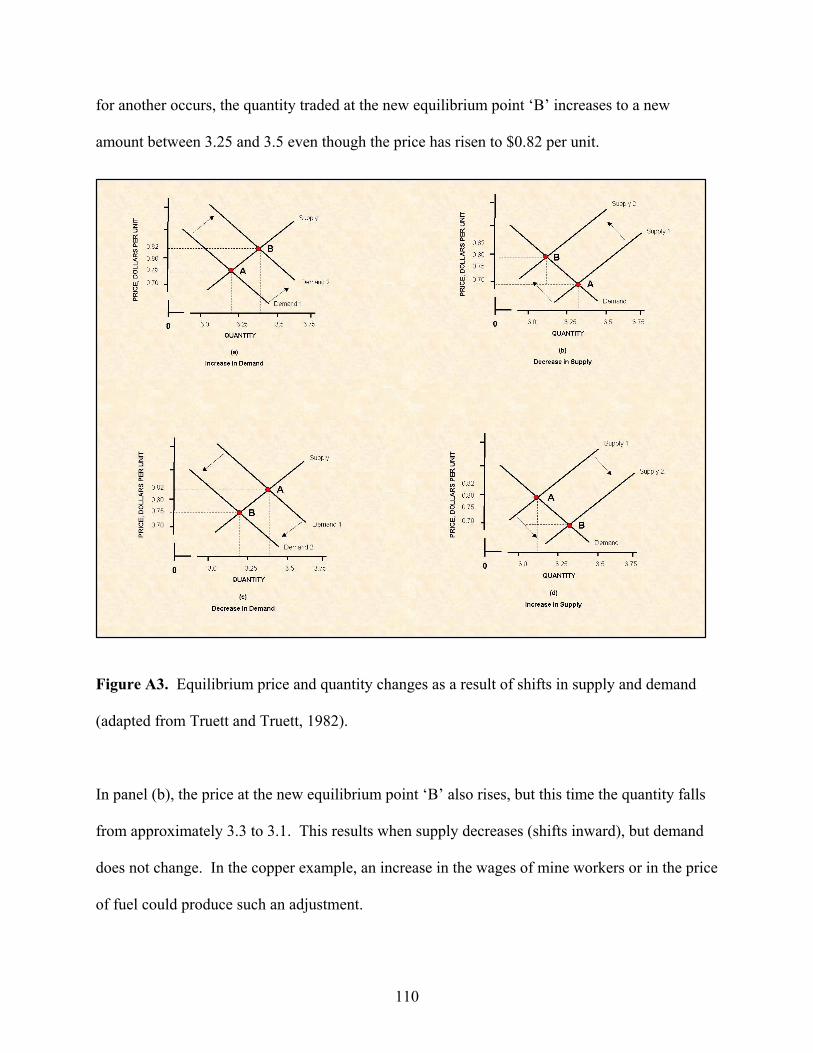
for another occurs, the quantity traded at the new equilibrium point ‘B’ increases to a new
amount between 3.25 and 3.5 even though the price has risen to $0.82 per unit.
Figure A3. Equilibrium price and quantity changes as a result of shifts in supply and demand
(adapted from Truett and Truett, 1982).
In panel (b), the price at the new equilibrium point ‘B’ also rises, but this time the quantity falls
from approximately 3.3 to 3.1. This results when supply decreases (shifts inward), but demand
does not change. In the copper example, an increase in the wages of mine workers or in the price
of fuel could produce such an adjustment.
110
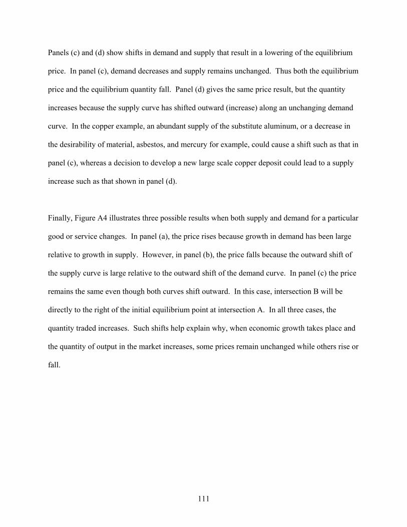
Panels (c) and (d) show shifts in demand and supply that result in a lowering of the equilibrium
price. In panel (c), demand decreases and supply remains unchanged. Thus both the equilibrium
price and the equilibrium quantity fall. Panel (d) gives the same price result, but the quantity
increases because the supply curve has shifted outward (increase) along an unchanging demand
curve. In the copper example, an abundant supply of the substitute aluminum, or a decrease in
the desirability of material, asbestos, and mercury for example, could cause a shift such as that in
panel (c), whereas a decision to develop a new large scale copper deposit could lead to a supply
increase such as that shown in panel (d).
Finally, Figure A4 illustrates three possible results when both supply and demand for a particular
good or service changes. In panel (a), the price rises because growth in demand has been large
relative to growth in supply. However, in panel (b), the price falls because the outward shift of
the supply curve is large relative to the outward shift of the demand curve. In panel (c) the price
remains the same even though both curves shift outward. In this case, intersection B will be
directly to the right of the initial equilibrium point at intersection A. In all three cases, the
quantity traded increases. Such shifts help explain why, when economic growth takes place and
the quantity of output in the market increases, some prices remain unchanged while others rise or
fall.
111
Figure A4. Equilibrium price or quantity impacts of supply or demand increases (adapted from
Truett and Truett, 1982).
112
References
Miller, R.L., 1998, Economics today—The micro view: New York, Addison-Wesley Publishing Company, Inc., 791 p. Rees, Judith, 1985, Natural resources allocation, economics and policy: New York, Methuen & Co., 449 p. Samuelson, P.A., 1961, Economics—An introductory analysis: New York, McGraw-Hill Book Company, Inc., 853 p. Truett, L.J., and Truett, D.B., 1982, Microeconomics: St. Paul, MN, West Publishing Co., 549 p.
113
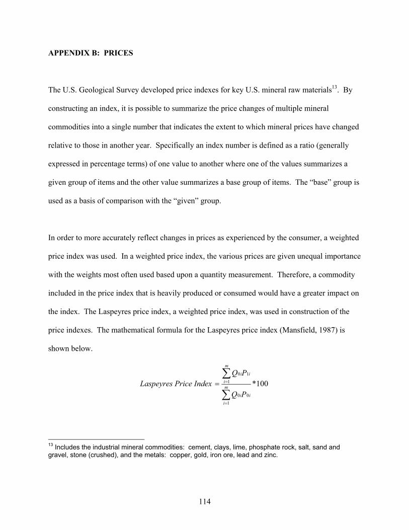
APPENDIX B: PRICES
The U.S. Geological Survey developed price indexes for key U.S. mineral raw materials13. By
constructing an index, it is possible to summarize the price changes of multiple mineral
commodities into a single number that indicates the extent to which mineral prices have changed
relative to those in another year. Specifically an index number is defined as a ratio (generally
expressed in percentage terms) of one value to another where one of the values summarizes a
given group of items and the other value summarizes a base group of items. The “base” group is
used as a basis of comparison with the “given” group.
In order to more accurately reflect changes in prices as experienced by the consumer, a weighted
price index was used. In a weighted price index, the various prices are given unequal importance
with the weights most often used based upon a quantity measurement. Therefore, a commodity
included in the price index that is heavily produced or consumed would have a greater impact on
the index. The Laspeyres price index, a weighted price index, was used in construction of the
price indexes. The mathematical formula for the Laspeyres price index (Mansfield, 1987) is
shown below.
Laspeyres Price Index 100*
100
110
∑
∑
=
== m
iii
m
iii
PQ
PQ
13 Includes the industrial mineral commodities: cement, clays, lime, phosphate rock, salt, sand and gravel, stone (crushed), and the metals: copper, gold, iron ore, lead and zinc.
114
where, Q0i = quantity of mineral commodity i produced (mined) in the base year (0) P1i = price of mineral commodity i for a given year (1) P0i = price of mineral commodity i for the base year (0)
and, i = 1 m, where m is a mineral commodity
Multiplying the price of each commodity in the given year by the quantity of that commodity
produced in the base year and then summing over all commodities derives the value in the given
year using given year prices and base year quantities. This sum is the numerator of the equation.
Multiplying the price of each commodity in the base year by the quantity produced in the base
year and then summing over all commodities derives the value of mineral production for these
commodities in the base year. This sum is the denominator of the equation. The result of the
division of the numerator by the denominator is an index that reflects relative changes in prices
for all of the included commodities with the weight of each commodity determined by its
quantity of production in the base year.
Therefore, by definition, the Laspeyres price index is the ratio, expressed as a percentage, of the
total value of raw mineral commodities produced in a given year based upon the quantity of each
raw mineral commodity produced in the base year to the total value of these same mineral
commodities in the base year.
The United States mine production14 composite price index (figure B1) was computed using data
for the seven highest total value of production industrial mineral commodities (cement, clay,
14 This index includes cement even though it is not mined but is the product of mined materials.
115
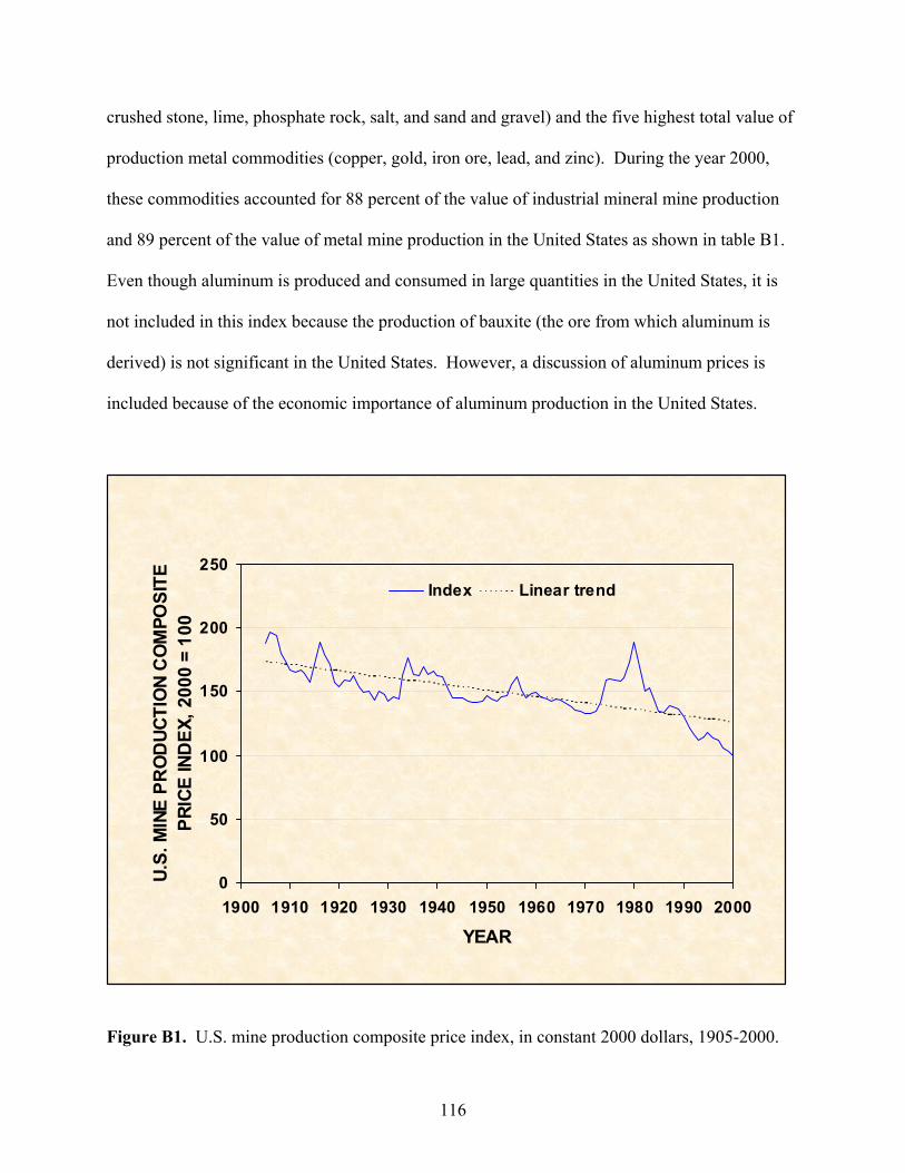
crushed stone, lime, phosphate rock, salt, and sand and gravel) and the five highest total value of
production metal commodities (copper, gold, iron ore, lead, and zinc). During the year 2000,
these commodities accounted for 88 percent of the value of industrial mineral mine production
and 89 percent of the value of metal mine production in the United States as shown in table B1.
Even though aluminum is produced and consumed in large quantities in the United States, it is
not included in this index because the production of bauxite (the ore from which aluminum is
derived) is not significant in the United States. However, a discussion of aluminum prices is
included because of the economic importance of aluminum production in the United States.
0
50
100
150
200
250
1900 1910 1920 1930 1940 1950 1960 1970 1980 1990 2000
YEAR
U.S.
MIN
E PR
OD
UCTI
ON
CO
MPO
SITE
PR
ICE
IND
EX, 2
000
= 10
0
Index Linear trend
Figure B1. U.S. mine production composite price index, in constant 2000 dollars, 1905-2000.
116
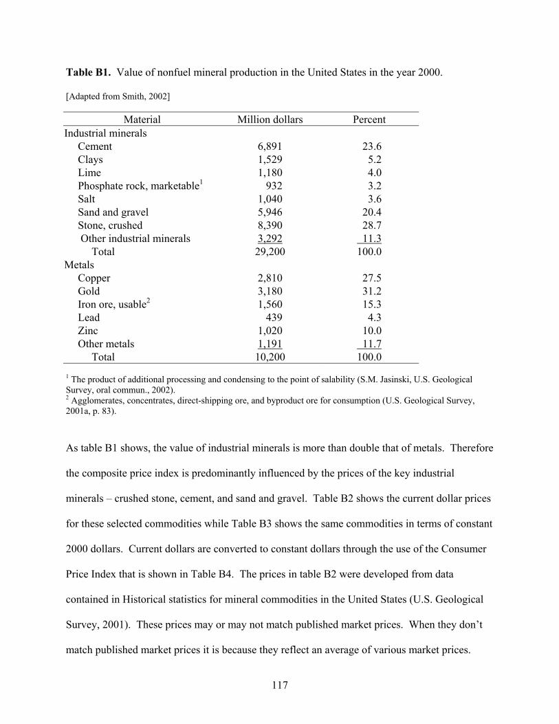
Table B1. Value of nonfuel mineral production in the United States in the year 2000.
[Adapted from Smith, 2002]
Material Million dollars Percent Industrial minerals Cement 6,891 23.6 Clays 1,529 5.2 Lime 1,180 4.0 Phosphate rock, marketable1 932 3.2 Salt 1,040 3.6 Sand and gravel 5,946 20.4 Stone, crushed 8,390 28.7 Other industrial minerals 3,292 11.3 Total 29,200 100.0 Metals Copper 2,810 27.5 Gold 3,180 31.2 Iron ore, usable2 1,560 15.3 Lead 439 4.3 Zinc 1,020 10.0 Other metals 1,191 11.7 Total 10,200 100.0 1 The product of additional processing and condensing to the point of salability (S.M. Jasinski, U.S. Geological Survey, oral commun., 2002). 2 Agglomerates, concentrates, direct-shipping ore, and byproduct ore for consumption (U.S. Geological Survey, 2001a, p. 83).
As table B1 shows, the value of industrial minerals is more than double that of metals. Therefore
the composite price index is predominantly influenced by the prices of the key industrial
minerals – crushed stone, cement, and sand and gravel. Table B2 shows the current dollar prices
for these selected commodities while Table B3 shows the same commodities in terms of constant
2000 dollars. Current dollars are converted to constant dollars through the use of the Consumer
Price Index that is shown in Table B4. The prices in table B2 were developed from data
contained in Historical statistics for mineral commodities in the United States (U.S. Geological
Survey, 2001). These prices may or may not match published market prices. When they don’t
match published market prices it is because they reflect an average of various market prices.
117
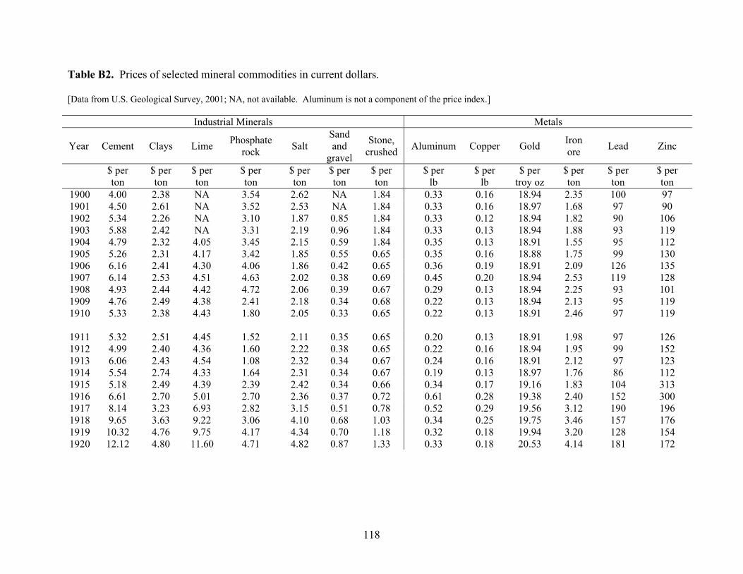
Table B2. Prices of selected mineral commodities in current dollars.
[Data from U.S. Geological Survey, 2001; NA, not available. Aluminum is not a component of the price index.]
Industrial Minerals Metals
Year Cement Clays Lime Phosphate rock Salt
Sand and
gravel
Stone, crushed Aluminum Copper Gold Iron
ore Lead Zinc
$ perton
$ per ton
$ per ton
$ per ton
$ per ton
$ per ton
$ per ton
$ per lb
$ per lb
$ per troy oz
$ per ton
$ per ton
$ per ton
1900 4.00 2.38 NA 3.54 2.62 NA 1.84 0.33 0.16 18.94 2.35 100 971901 4.50 2.61 NA 3.52 2.53 NA 1.84 0.33 0.16 18.97 1.68 97 901902 5.34 2.26 NA 3.10 1.87 0.85 1.84 0.33 0.12 18.94 1.82 90 1061903 5.88 2.42 NA 3.31 2.19 0.96 1.84 0.33 0.13 18.94 1.88 93 1191904 4.79 2.32 4.05 3.45 2.15 0.59 1.84 0.35 0.13 18.91 1.55 95 1121905 5.26 2.31 4.17 3.42 1.85 0.55 0.65 0.35 0.16 18.88 1.75 99 1301906 6.16 2.41 4.30 4.06 1.86 0.42 0.65 0.36 0.19 18.91 2.09 126 1351907 6.14 2.53 4.51 4.63 2.02 0.38 0.69 0.45 0.20 18.94 2.53 119 1281908 4.93 2.44 4.42 4.72 2.06 0.39 0.67 0.29 0.13 18.94 2.25 93 1011909 4.76 2.49 4.38 2.41 2.18 0.34 0.68 0.22 0.13 18.94 2.13 95 1191910 5.33 2.38 4.43 1.80 2.05 0.33 0.65 0.22 0.13 18.91 2.46 97 119
1911 5.32 2.51 4.45 1.52 2.11 0.35 0.65 0.20 0.13 18.91 1.98 97 1261912 4.99 2.40 4.36 1.60 2.22 0.38 0.65 0.22 0.16 18.94 1.95 99 1521913 6.06 2.43 4.54 1.08 2.32 0.34 0.67 0.24 0.16 18.91 2.12 97 1231914 5.54 2.74 4.33 1.64 2.31 0.34 0.67 0.19 0.13 18.97 1.76 86 1121915 5.18 2.49 4.39 2.39 2.42 0.34 0.66 0.34 0.17 19.16 1.83 104 3131916 6.61 2.70 5.01 2.70 2.36 0.37 0.72 0.61 0.28 19.38 2.40 152 3001917 8.14 3.23 6.93 2.82 3.15 0.51 0.78 0.52 0.29 19.56 3.12 190 1961918 9.65 3.63 9.22 3.06 4.10 0.68 1.03 0.34 0.25 19.75 3.46 157 1761919 10.32 4.76 9.75 4.17 4.34 0.70 1.18 0.32 0.18 19.94 3.20 128 1541920 12.12 4.80 11.60 4.71 4.82 0.87 1.33 0.33 0.18 20.53 4.14 181 172
118

Table B2. Prices of selected mineral commodities in current dollars-Continued.
Industrial Minerals Metals
Year Cement Clays Lime Phosphate rock Salt
Sand and
gravel
Stone, crushed Aluminum Copper Gold Iron
ore Lead Zinc
$ perton
$ per ton
$ per ton
$ per ton
$ per ton
$ per ton
$ per ton
$ per lb
$ per lb
$ per troy oz
$ per ton
$ per ton
$ per ton
1921 11.22 5.02 10.80 3.68 5.43 0.78 1.31 0.22 0.13 20.59 3.00 104 1041922 10.38 4.86 10.10 2.73 4.46 0.80 1.17 0.19 0.14 20.75 3.32 126 1261923 11.13 4.66 10.80 2.65 4.30 0.77 1.27 0.25 0.15 20.65 3.44 163 1481924 10.50 4.42 10.70 2.53 4.17 0.69 1.19 0.27 0.13 20.68 2.83 183 1391925 10.20 4.48 10.30 2.22 3.90 0.69 1.16 0.27 0.14 20.65 2.57 201 1691926 9.89 4.96 10.00 2.64 3.75 0.67 1.25 0.27 0.14 20.62 2.52 186 1631927 9.43 4.90 9.65 2.94 3.61 0.64 1.13 0.25 0.13 20.65 2.50 150 1381928 9.11 4.87 9.01 3.13 3.65 0.66 1.23 0.24 0.15 20.68 2.45 139 1331929 8.66 4.78 8.64 3.04 3.53 0.66 1.10 0.24 0.18 20.62 2.65 151 1431930 8.42 4.60 8.33 3.15 3.42 0.65 1.08 0.24 0.13 20.59 2.47 122 101
1931 6.51 4.57 7.60 3.19 3.23 0.63 1.11 0.23 0.08 22.49 2.36 94 801932 5.95 4.80 6.92 2.70 3.43 0.54 1.04 0.23 0.06 20.68 1.41 70 641933 7.83 4.63 6.92 2.60 3.23 0.55 0.96 0.23 0.07 26.34 3.52 85 891934 9.06 4.64 7.89 2.72 3.31 0.58 1.10 0.23 0.09 34.84 2.64 85 921935 8.81 4.42 8.03 2.64 3.04 0.55 0.99 0.20 0.09 34.84 2.66 90 961936 8.61 4.28 7.92 2.13 2.78 0.56 1.01 0.21 0.10 34.84 2.64 104 1081937 8.45 4.45 8.04 2.45 2.88 0.57 1.12 0.20 0.13 34.84 2.82 132 1441938 8.26 4.99 7.95 2.42 3.19 0.53 1.07 0.20 0.10 34.84 2.56 104 1021939 8.43 4.68 7.79 2.48 2.91 0.52 1.03 0.20 0.11 34.52 2.99 111 1131940 8.45 4.30 7.66 2.57 2.82 0.51 1.02 0.19 0.12 33.90 2.52 114 140
119
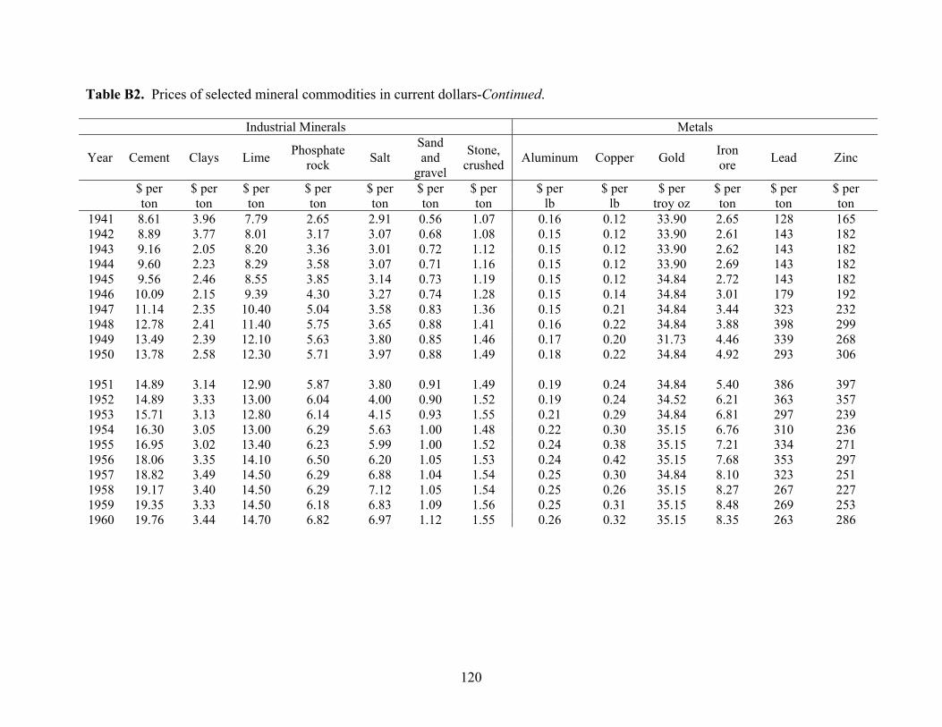
Table B2. Prices of selected mineral commodities in current dollars-Continued.
Industrial Minerals Metals
Cement Clays Lime Phosphate rock Salt
Sand and
gravel
Stone, crushed Aluminum Copper Gold Iron
ore Lead Zinc
$ per ton
$ per ton
$ per ton
$ per ton
$ per ton
$ per ton
$ per lb
$ per lb
$ per troy oz
$ per ton
$ per $ per ton
1941 8.61 3.96 7.79 2.65 2.91 0.56 1.07 0.16 0.12 33.90 128 1651942 8.89 3.77 8.01 3.17 3.07 0.68 1.08 0.15 0.12 33.90 143 1821943 9.16 2.05 8.20 3.36 3.01 0.72 1.12 0.15 0.12 33.90 143 1821944 9.60 2.23 8.29 3.58 3.07 0.71 1.16 0.15 0.12 33.90 143 1821945 9.56 2.46 8.55 3.85 3.14 0.73 1.19 0.15 0.12 34.84 143 1821946 10.09 2.15 9.39 4.30 3.27 0.74 1.28 0.15 0.14 34.84 179 1921947 11.14 2.35 10.40 5.04 3.58 0.83 1.36 0.15 0.21 34.84 323 2321948 12.78 2.41 11.40 5.75 3.65 0.88 1.41 0.16 0.22 34.84 398 2991949 13.49 2.39 12.10 5.63 3.80 0.85 1.46 0.17 0.20 31.73 339 2681950 13.78 2.58 12.30 5.71 3.97 0.88 1.49 0.18 0.22 34.84 293 306
Year
$ perton ton
2.652.612.622.692.723.013.443.884.464.92
1951 14.89 3.14 12.90 5.87 3.80 0.91 1.49 0.19 0.24 34.84 5.40 386 3971952 14.89 3.33 13.00 6.04 4.00 0.90 1.52 0.19 0.24 34.52 6.21 363 3571953 15.71 3.13 12.80 6.14 4.15 0.93 1.55 0.21 0.29 34.84 6.81 297 2391954 16.30 3.05 13.00 6.29 5.63 1.00 1.48 0.22 0.30 35.15 6.76 310 2361955 16.95 3.02 13.40 6.23 5.99 1.00 1.52 0.24 0.38 35.15 7.21 334 2711956 18.06 3.35 14.10 6.50 6.20 1.05 1.53 0.24 0.42 35.15 7.68 353 2971957 18.82 3.49 14.50 6.29 6.88 1.04 1.54 0.25 0.30 34.84 8.10 323 2511958 19.17 3.40 14.50 6.29 7.12 1.05 1.54 0.25 0.26 35.15 8.27 267 2271959 19.35 3.33 14.50 6.18 6.83 1.09 1.56 0.25 0.31 35.15 8.48 269 2531960 19.76 3.44 14.70 6.82 6.97 1.12 1.55 0.26 0.32 35.15 8.35 263 286
120
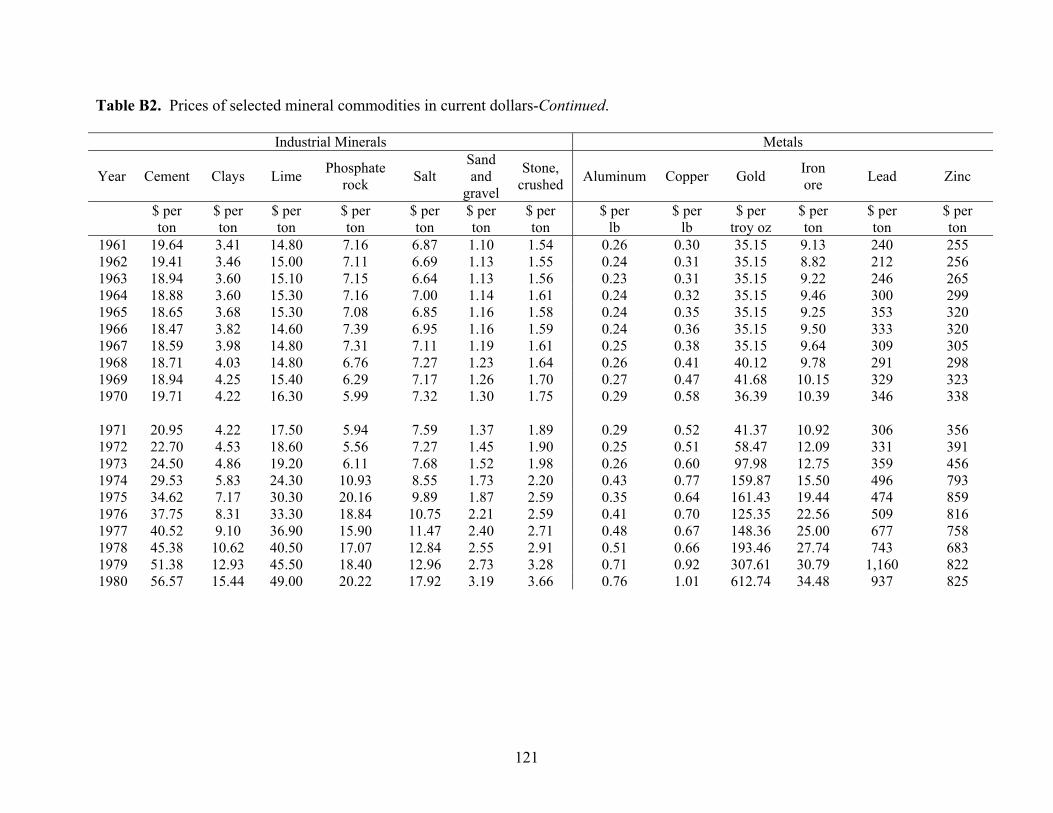
Table B2. Prices of selected mineral commodities in current dollars-Continued.
Industrial Minerals Metals
Year Cement Clays Lime Phosphate rock Salt
Sand and
gravel
Stone, crushed Aluminum Copper Gold Iron
ore Lead Zinc
$ perton
$ per ton
$ per ton
$ per ton
$ per ton
$ per ton
$ per ton
$ per lb
$ per lb
$ per troy oz
$ per ton
$ per ton
$ per ton
1961 19.64 3.41 14.80 7.16 6.87 1.10 1.54 0.26 0.30 35.15 9.13 240 2551962 19.41 3.46 15.00 7.11 6.69 1.13 1.55 0.24 0.31 35.15 8.82 212 2561963 18.94 3.60 15.10 7.15 6.64 1.13 1.56 0.23 0.31 35.15 9.22 246 2651964 18.88 3.60 15.30 7.16 7.00 1.14 1.61 0.24 0.32 35.15 9.46 300 2991965 18.65 3.68 15.30 7.08 6.85 1.16 1.58 0.24 0.35 35.15 9.25 353 3201966 18.47 3.82 14.60 7.39 6.95 1.16 1.59 0.24 0.36 35.15 9.50 333 3201967 18.59 3.98 14.80 7.31 7.11 1.19 1.61 0.25 0.38 35.15 9.64 309 3051968 18.71 4.03 14.80 6.76 7.27 1.23 1.64 0.26 0.41 40.12 9.78 291 2981969 18.94 4.25 15.40 6.29 7.17 1.26 1.70 0.27 0.47 41.68 10.15 329 3231970 19.71 4.22 16.30 5.99 7.32 1.30 1.75 0.29 0.58 36.39 10.39 346 338
1971 20.95 4.22 17.50 5.94 7.59 1.37 1.89 0.29 0.52 41.37 10.92 306 3561972 22.70 4.53 18.60 5.56 7.27 1.45 1.90 0.25 0.51 58.47 12.09 331 3911973 24.50 4.86 19.20 6.11 7.68 1.52 1.98 0.26 0.60 97.98 12.75 359 4561974 29.53 5.83 24.30 10.93 8.55 1.73 2.20 0.43 0.77 159.87 15.50 496 7931975 34.62 7.17 30.30 20.16 9.89 1.87 2.59 0.35 0.64 161.43 19.44 474 8591976 37.75 8.31 33.30 18.84 10.75 2.21 2.59 0.41 0.70 125.35 22.56 509 8161977 40.52 9.10 36.90 15.90 11.47 2.40 2.71 0.48 0.67 148.36 25.00 677 7581978 45.38 10.62 40.50 17.07 12.84 2.55 2.91 0.51 0.66 193.46 27.74 743 6831979 51.38 12.93 45.50 18.40 12.96 2.73 3.28 0.71 0.92 307.61 30.79 1,160 8221980 56.57 15.44 49.00 20.22 17.92 3.19 3.66 0.76 1.01 612.74 34.48 937 825
121
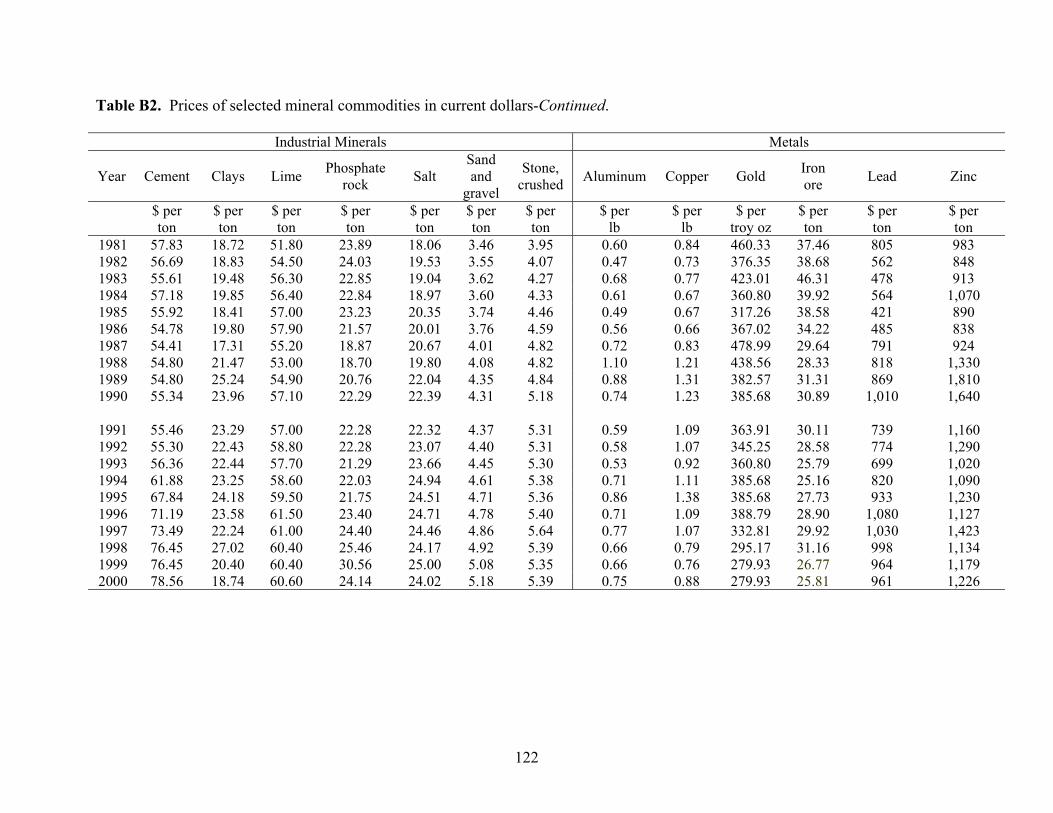
Table B2. Prices of selected mineral commodities in current dollars-Continued.
Industrial Minerals Metals
Year Cement Clays Lime Phosphate rock Salt
Sand and
gravel
Stone, crushed Aluminum Copper Gold Iron
ore Lead Zinc
$ perton
$ per ton
$ per ton
$ per ton
$ per ton
$ per ton
$ per ton
$ per lb
$ per lb
$ per troy oz
$ per ton
$ per ton
$ per ton
1981 57.83 18.72 51.80 23.89 18.06 3.46 3.95 0.60 0.84 460.33 37.46 805 9831982 56.69 18.83 54.50 24.03 19.53 3.55 4.07 0.47 0.73 376.35 38.68 562 8481983 55.61 19.48 56.30 22.85 19.04 3.62 4.27 0.68 0.77 423.01 46.31 478 9131984 57.18 19.85 56.40 22.84 18.97 3.60 4.33 0.61 0.67 360.80 39.92 564 1,0701985 55.92 18.41 57.00 23.23 20.35 3.74 4.46 0.49 0.67 317.26 38.58 421 8901986 54.78 19.80 57.90 21.57 20.01 3.76 4.59 0.56 0.66 367.02 34.22 485 8381987 54.41 17.31 55.20 18.87 20.67 4.01 4.82 0.72 0.83 478.99 29.64 791 9241988 54.80 21.47 53.00 18.70 19.80 4.08 4.82 1.10 1.21 438.56 28.33 818 1,3301989 54.80 25.24 54.90 20.76 22.04 4.35 4.84 0.88 1.31 382.57 31.31 869 1,8101990 55.34 23.96 57.10 22.29 22.39 4.31 5.18 0.74 1.23 385.68 30.89 1,010 1,640
1991 55.46 23.29 57.00 22.28 22.32 4.37 5.31 0.59 1.09 363.91 30.11 739 1,1601992 55.30 22.43 58.80 22.28 23.07 4.40 5.31 0.58 1.07 345.25 28.58 774 1,2901993 56.36 22.44 57.70 21.29 23.66 4.45 5.30 0.53 0.92 360.80 25.79 699 1,0201994 61.88 23.25 58.60 22.03 24.94 4.61 5.38 0.71 1.11 385.68 25.16 820 1,0901995 67.84 24.18 59.50 21.75 24.51 4.71 5.36 0.86 1.38 385.68 27.73 933 1,2301996 71.19 23.58 61.50 23.40 24.71 4.78 5.40 0.71 1.09 388.79 28.90 1,080 1,1271997 73.49 22.24 61.00 24.40 24.46 4.86 5.64 0.77 1.07 332.81 29.92 1,030 1,4231998 76.45 27.02 60.40 25.46 24.17 4.92 5.39 0.66 0.79 295.17 31.16 998 1,1341999 76.45 20.40 60.40 30.56 25.00 5.08 5.35 0.66 0.76 279.93 26.77 964 1,1792000 78.56 18.74 60.60 24.14 24.02 5.18 5.39 0.75 0.88 279.93 25.81 961 1,226
122
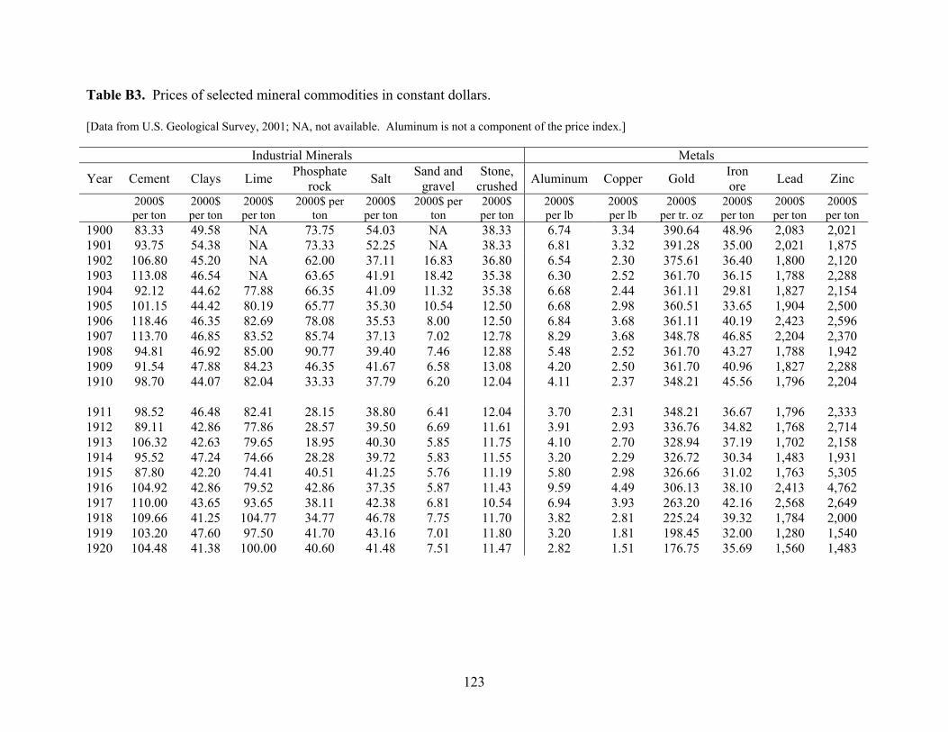
Table B3. Prices of selected mineral commodities in constant dollars.
[Data from U.S. Geological Survey, 2001; NA, not available. Aluminum is not a component of the price index.]
Industrial Minerals Metals
Year Cement Clays Lime Phosphate rock Salt Sand and
gravel Stone,
crushed Aluminum Copper Gold Iron ore Lead Zinc
2000$per ton
2000$ per ton
2000$ per ton
2000$ per ton
2000$ per ton
2000$ per ton
2000$ per ton
2000$ per lb
2000$ per lb
2000$ per tr. oz
2000$ per ton
2000$ per ton
2000$ per ton
1900 83.33 49.58 NA 73.75 54.03 NA 38.33 6.74 3.34 390.64 48.96 2,083 2,0211901 93.75 54.38 NA 73.33 52.25 NA 38.33 6.81 3.32 391.28 35.00 2,021 1,8751902 106.80 45.20 NA 62.00 37.11 16.83 36.80 6.54 2.30 375.61 36.40 1,800 2,1201903 113.08 46.54 NA 63.65 41.91 18.42 35.38 6.30 2.52 361.70 36.15 1,788 2,2881904 92.12 44.62 77.88 66.35 41.09 11.32 35.38 6.68 2.44 361.11 29.81 1,827 2,1541905 101.15 44.42 80.19 65.77 35.30 10.54 12.50 6.68 2.98 360.51 33.65 1,904 2,5001906 118.46 46.35 82.69 78.08 35.53 8.00 12.50 6.84 3.68 361.11 40.19 2,423 2,5961907 113.70 46.85 83.52 85.74 37.13 7.02 12.78 8.29 3.68 348.78 46.85 2,204 2,3701908 94.81 46.92 85.00 90.77 39.40 7.46 12.88 5.48 2.52 361.70 43.27 1,788 1,9421909 91.54 47.88 84.23 46.35 41.67 6.58 13.08 4.20 2.50 361.70 40.96 1,827 2,2881910 98.70 44.07 82.04 33.33 37.79 6.20 12.04 4.11 2.37 348.21 45.56 1,796 2,204
1911 98.52 46.48 82.41 28.15 38.80 6.41 12.04 3.70 2.31 348.21 36.67 1,796 2,3331912 89.11 42.86 77.86 28.57 39.50 6.69 11.61 3.91 2.93 336.76 34.82 1,768 2,7141913 106.32 42.63 79.65 18.95 40.30 5.85 11.75 4.10 2.70 328.94 37.19 1,702 2,1581914 95.52 47.24 74.66 28.28 39.72 5.83 11.55 3.20 2.29 326.72 30.34 1,483 1,9311915 87.80 42.20 74.41 40.51 41.25 5.76 11.19 5.80 2.98 326.66 31.02 1,763 5,3051916 104.92 42.86 79.52 42.86 37.35 5.87 11.43 9.59 4.49 306.13 38.10 2,413 4,7621917 110.00 43.65 93.65 38.11 42.38 6.81 10.54 6.94 3.93 263.20 42.16 2,568 2,6491918 109.66 41.25 104.77 34.77 46.78 7.75 11.70 3.82 2.81 225.24 39.32 1,784 2,0001919 103.20 47.60 97.50 41.70 43.16 7.01 11.80 3.20 1.81 198.45 32.00 1,280 1,5401920 104.48 41.38 100.00 40.60 41.48 7.51 11.47 2.82 1.51 176.75 35.69 1,560 1,483
123
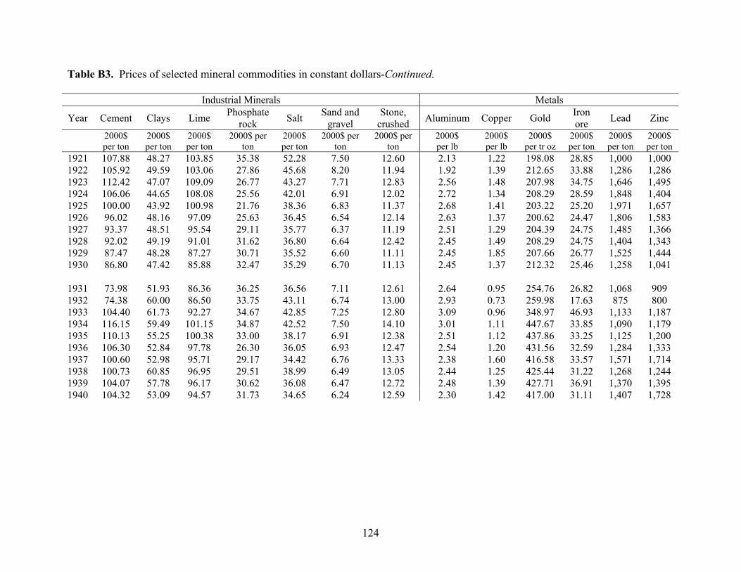
Table B3. Prices of selected mineral commodities in constant dollars-Continued.
Industrial Minerals Metals
Year Cement Clays Lime Phosphate rock Salt Sand and
gravel Stone,
crushed Aluminum Copper Gold Iron ore Lead Zinc
2000$per ton
2000$ per ton
2000$ per ton
2000$ per ton
2000$ per ton
2000$ per ton
2000$ per ton
2000$ per lb
2000$ per lb
2000$ per tr oz
2000$ per ton
2000$ per ton
2000$ per ton
1921 107.88 48.27 103.85 35.38 52.28 7.50 12.60 2.13 1.22 198.08 28.85 1,000 1,0001922 105.92 49.59 103.06 27.86 45.68 8.20 11.94 1.92 1.39 212.65 33.88 1,286 1,2861923 112.42 47.07 109.09 26.77 43.27 7.71 12.83 2.56 1.48 207.98 34.75 1,646 1,4951924 106.06 44.65 108.08 25.56 42.01 6.91 12.02 2.72 1.34 208.29 28.59 1,848 1,4041925 100.00 43.92 100.98 21.76 38.36 6.83 11.37 2.68 1.41 203.22 25.20 1,971 1,6571926 96.02 48.16 97.09 25.63 36.45 6.54 12.14 2.63 1.37 200.62 24.47 1,806 1,5831927 93.37 48.51 95.54 29.11 35.77 6.37 11.19 2.51 1.29 204.39 24.75 1,485 1,3661928 92.02 49.19 91.01 31.62 36.80 6.64 12.42 2.45 1.49 208.29 24.75 1,404 1,3431929 87.47 48.28 87.27 30.71 35.52 6.60 11.11 2.45 1.85 207.66 26.77 1,525 1,4441930 86.80 47.42 85.88 32.47 35.29 6.70 11.13 2.45 1.37 212.32 25.46 1,258 1,041
1931 73.98 51.93 86.36 36.25 36.56 7.11 12.61 2.64 0.95 254.76 26.82 1,068 9091932 74.38 60.00 86.50 33.75 43.11 6.74 13.00 2.93 0.73 259.98 17.63 875 8001933 104.40 61.73 92.27 34.67 42.85 7.25 12.80 3.09 0.96 348.97 46.93 1,133 1,1871934 116.15 59.49 101.15 34.87 42.52 7.50 14.10 3.01 1.11 447.67 33.85 1,090 1,1791935 110.13 55.25 100.38 33.00 38.17 6.91 12.38 2.51 1.12 437.86 33.25 1,125 1,2001936 106.30 52.84 97.78 26.30 36.05 6.93 12.47 2.54 1.20 431.56 32.59 1,284 1,3331937 100.60 52.98 95.71 29.17 34.42 6.76 13.33 2.38 1.60 416.58 33.57 1,571 1,7141938 100.73 60.85 96.95 29.51 38.99 6.49 13.05 2.44 1.25 425.44 31.22 1,268 1,2441939 104.07 57.78 96.17 30.62 36.08 6.47 12.72 2.48 1.39 427.71 36.91 1,370 1,3951940 104.32 53.09 94.57 31.73 34.65 6.24 12.59 2.30 1.42 417.00 31.11 1,407 1,728
124
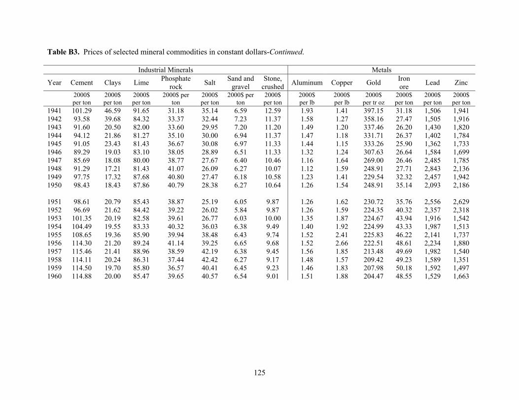
Table B3. Prices of selected mineral commodities in constant dollars-Continued.
Industrial Minerals Metals
Year Cement Clays Lime Phosphate rock Salt Sand and
gravel Stone,
crushed Aluminum Copper Gold Iron ore Lead Zinc
2000$per ton
2000$ per ton
2000$ per ton
2000$ per ton
2000$ per ton
2000$ per ton
2000$ per ton
2000$ per lb
2000$ per lb
2000$ per tr oz
2000$ per ton
2000$ per ton
2000$ per ton
1941 101.29 46.59 91.65 31.18 35.14 6.59 12.59 1.93 1.41 397.15 31.18 1,506 1,9411942 93.58 39.68 84.32 33.37 32.44 7.23 11.37 1.58 1.27 358.16 27.47 1,505 1,9161943 91.60 20.50 82.00 33.60 29.95 7.20 11.20 1.49 1.20 337.46 26.20 1,430 1,8201944 94.12 21.86 81.27 35.10 30.00 6.94 11.37 1.47 1.18 331.71 26.37 1,402 1,7841945 91.05 23.43 81.43 36.67 30.08 6.97 11.33 1.44 1.15 333.26 25.90 1,362 1,7331946 89.29 19.03 83.10 38.05 28.89 6.51 11.33 1.32 1.24 307.63 26.64 1,584 1,6991947 85.69 18.08 80.00 38.77 27.67 6.40 10.46 1.16 1.64 269.00 26.46 2,485 1,7851948 91.29 17.21 81.43 41.07 26.09 6.27 10.07 1.12 1.59 248.91 27.71 2,843 2,1361949 97.75 17.32 87.68 40.80 27.47 6.18 10.58 1.23 1.41 229.54 32.32 2,457 1,9421950 98.43 18.43 87.86 40.79 28.38 6.27 10.64 1.26 1.54 248.91 35.14 2,093 2,186
1951 98.61 20.79 85.43 38.87 25.19 6.05 9.87 1.26 1.62 230.72 35.76 2,556 2,6291952 96.69 21.62 84.42 39.22 26.02 5.84 9.87 1.26 1.59 224.35 40.32 2,357 2,3181953 101.35 20.19 82.58 39.61 26.77 6.03 10.00 1.35 1.87 224.67 43.94 1,916 1,5421954 104.49 19.55 83.33 40.32 36.03 6.38 9.49 1.40 1.92 224.99 43.33 1,987 1,5131955 108.65 19.36 85.90 39.94 38.48 6.43 9.74 1.52 2.41 225.83 46.22 2,141 1,7371956 114.30 21.20 89.24 41.14 39.25 6.65 9.68 1.52 2.66 222.51 48.61 2,234 1,8801957 115.46 21.41 88.96 38.59 42.19 6.38 9.45 1.56 1.85 213.48 49.69 1,982 1,5401958 114.11 20.24 86.31 37.44 42.42 6.27 9.17 1.48 1.57 209.42 49.23 1,589 1,3511959 114.50 19.70 85.80 36.57 40.41 6.45 9.23 1.46 1.83 207.98 50.18 1,592 1,4971960 114.88 20.00 85.47 39.65 40.57 6.54 9.01 1.51 1.88 204.47 48.55 1,529 1,663
125
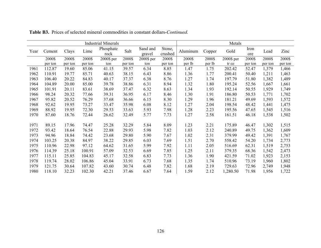
Table B3. Prices of selected mineral commodities in constant dollars-Continued.
Industrial Minerals Metals
Year Cement Clays Lime Phosphate rock Salt Sand and
gravel Stone,
crushed Aluminum Copper Gold Iron ore Lead Zinc
2000$per ton
2000$ per ton
2000$ per ton
2000$ per ton
2000$ per ton
2000$ per ton
2000$ per ton
2000$ per lb
2000$ per lb
2000$ per tr oz
2000$ per ton
2000$ per ton
2000$ per ton
1961 112.87 19.60 85.06 41.15 39.57 6.34 8.85 1.47 1.75 202.42 52.47 1,379 1,4661962 110.91 19.77 85.71 40.63 38.15 6.43 8.86 1.36 1.77 200.41 50.40 1,211 1,4631963 106.40 20.22 84.83 40.17 37.37 6.38 8.76 1.27 1.74 197.79 51.80 1,382 1,4891964 104.89 20.00 85.00 39.78 38.86 6.31 8.94 1.32 1.80 195.24 52.56 1,667 1,6611965 101.91 20.11 83.61 38.69 37.47 6.32 8.63 1.34 1.93 192.14 50.55 1,929 1,7491966 98.24 20.32 77.66 39.31 36.95 6.17 8.46 1.30 1.91 186.80 50.53 1,771 1,7021967 95.82 20.52 76.29 37.68 36.66 6.15 8.30 1.29 1.96 181.21 49.69 1,593 1,5721968 92.62 19.95 73.27 33.47 35.98 6.08 8.12 1.27 2.04 198.54 48.42 1,441 1,4751969 88.92 19.95 72.30 29.53 33.63 5.93 7.98 1.28 2.23 195.56 47.65 1,545 1,5161970 87.60 18.76 72.44 26.62 32.49 5.77 7.73 1.27 2.58 161.51 46.18 1,538 1,502
1971 89.15 17.96 74.47 25.28 32.29 5.84 8.09 1.23 2.21 175.89 46.47 1,302 1,5151972 93.42 18.64 76.54 22.88 29.93 5.98 7.82 1.03 2.12 240.89 49.75 1,362 1,6091973 94.96 18.84 74.42 23.68 29.80 5.90 7.67 1.02 2.31 379.99 49.42 1,391 1,7671974 103.25 20.38 84.97 38.22 29.85 6.03 7.69 1.51 2.70 558.42 54.20 1,734 2,7731975 110.96 22.98 97.12 64.62 31.65 5.99 7.92 1.11 2.05 516.69 62.31 1,519 2,7531976 114.39 25.18 100.91 57.09 32.53 6.69 7.85 1.25 2.11 379.35 68.36 1,542 2,4731977 115.11 25.85 104.83 45.17 32.58 6.83 7.73 1.36 1.90 421.59 71.02 1,923 2,1531978 119.74 28.02 106.86 45.04 33.91 6.73 7.68 1.35 1.74 510.96 73.19 1,960 1,8021979 121.75 30.64 107.82 43.60 30.74 6.48 7.82 1.68 2.19 729.63 72.96 2,749 1,9481980 118.10 32.23 102.30 42.21 37.46 6.67 7.64 1.59 2.12 1,280.50 71.98 1,956 1,722
126
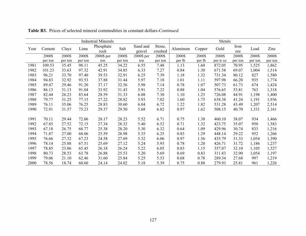
Table B3. Prices of selected mineral commodities in constant dollars-Continued.
Industrial Minerals Metals
Year Cement Clays Lime Phosphate rock Salt Stone,
crushed Aluminum Copper Gold Iron ore Lead Zinc
2000$per ton
2000$ per ton
2000$ per ton
2000$ per ton
2000$ per ton
2000$ per ton
2000$ per lb
2000$ per lb
2000$ per tr oz
2000$ per ton
2000$ per ton
2000$ per ton
1981 109.53 35.45 98.11 45.25 6.55 7.48 1.13 1.60 872.05 70.95 1,525 1,8621982 101.23 33.63 97.32 42.91 6.33 7.27 0.84 1.30 671.58 69.07 1,004 1,5141983 96.21 33.70 97.40 39.53 6.25 7.39 1.18 1.32 731.34 80.12 827 1,5801984 94.83 32.92 93.53 37.88
Sand and gravel
2000$ per ton
34.2234.8532.9131.44 5.97 7.18 1.01 1.11 597.98 66.20 935 1,774
1985 89.47 29.46 91.20 37.17 32.56 5.98 7.14 0.78 1.07 507.73 61.73 674 1,4241986 86.13 31.13 91.04 33.92 31.43 5.91 7.22 0.88 1.04 576.65 53.81 763 1,3181987 82.44 26.23 83.64 28.59 31.33 6.08 7.30 1.10 1.25 726.08 44.91 1,198 1,4001988 79.77 31.25 77.15 27.22 28.82 5.93 7.02 1.60 1.75 638.38 41.24 1,191 1,9361989 76.11 35.06 76.25 28.83 30.60 6.04 6.72 1.22 1.82 531.28 43.49 1,207 2,5141990 72.91 31.57
75.23
29.37 29.50
5.68 6.82 0.97 1.62 508.15
40.70 1,331 2,161
1991 70.11 29.44 72.06 28.17 28.23 5.52 6.71 0.75 1.38 460.10 38.07 934 1,4661992 67.85 27.52 72.15 27.34 28.32 5.40 6.52 0.71 1.32 423.75 35.07 950 1,5831993 67.18 26.75 68.77 25.38 28.20 5.30 6.32 0.64 1.09 429.96 30.74 833 1,2161994 71.87 68.06 25.59 28.98 5.35 6.25 0.83 1.29 448.14 29.22 952 1,2661995 76.66 27.32 67.23 24.58 27.69 5.32 6.06 0.97 1.56 435.79 31.33 1,054 1,3901996 78.14 25.88 67.51 25.69 27.12 5.24 5.93 0.78 1.20 426.71 31.72 1,186 1,2371997 78.85 23.86 65.45 26.18 26.24 5.22 6.05 0.83 1.15 357.07 32.10 1,105 1,5271998 80.73 28.53 63.78 26.88 25.53 5.20 5.69 0.69 0.83 311.83 32.90 1,054 1,1971999 79.06 21.10 62.46 31.60 25.84 5.25 5.53 0.68 0.78 289.34 27.68 997 1,2192000 78.56 18.74 60.60 24.14 24.02 5.18 5.39 0.75 0.88 279.93 25.81 961 1,226
27.00
127
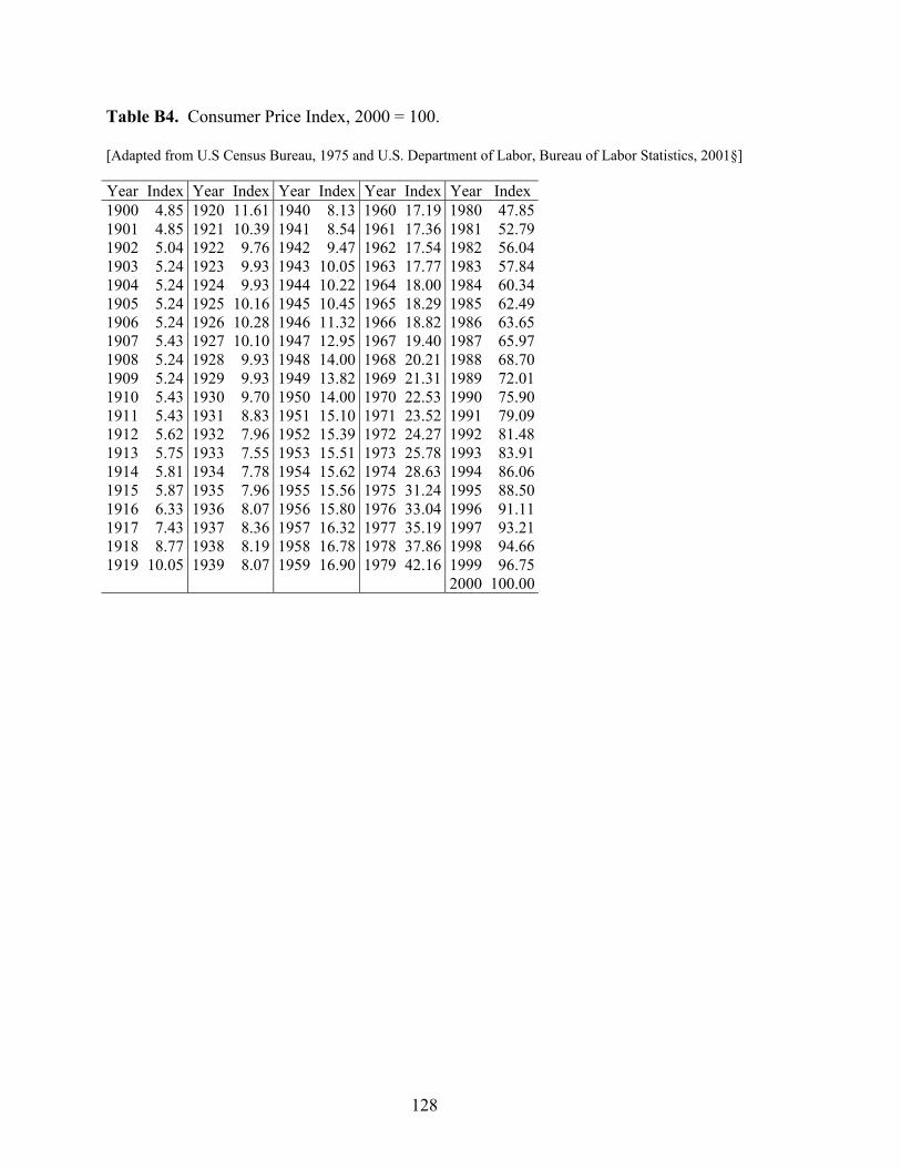
Table B4. Consumer Price Index, 2000 = 100.
[Adapted from U.S Census Bureau, 1975 and U.S. Department of Labor, Bureau of Labor Statistics, 2001§]
Year Index Year Index Year Index Year Index Year Index1900 4.85 1920 11.61 1940 8.13 1960 17.19 1980 47.851901 4.85 1921 10.39 1941 8.54 1961 17.36 1981 52.791902 5.04 1922 9.76 1942 9.47 1962 17.54 1982 56.041903 5.24 1923 9.93 1943 10.05 1963 17.77 1983 57.841904 5.24 1924 9.93 1944 10.22 1964 18.00 1984 60.341905 5.24 1925 10.16 1945 10.45 1965 18.29 1985 62.491906 5.24 1926 10.28 1946 11.32 1966 18.82 1986 63.651907 5.43 1927 10.10 1947 12.95 1967 19.40 1987 65.971908 5.24 1928 9.93 1948 14.00 1968 20.21 1988 68.701909 5.24 1929 9.93 1949 13.82 1969 21.31 1989 72.011910 5.43 1930 9.70 1950 14.00 1970 22.53 1990 75.901911 5.43 1931 8.83 1951 15.10 1971 23.52 1991 79.091912 5.62 1932 7.96 1952 15.39 1972 24.27 1992 81.481913 5.75 1933 7.55 1953 15.51 1973 25.78 1993 83.911914 5.81 1934 7.78 1954 15.62 1974 28.63 1994 86.061915 5.87 1935 7.96 1955 15.56 1975 31.24 1995 88.501916 6.33 1936 8.07 1956 15.80 1976 33.04 1996 91.111917 7.43 1937 8.36 1957 16.32 1977 35.19 1997 93.211918 8.77 1938 8.19 1958 16.78 1978 37.86 1998 94.661919 10.05 1939 8.07 1959 16.90 1979 42.16 1999 96.75
2000 100.00
128
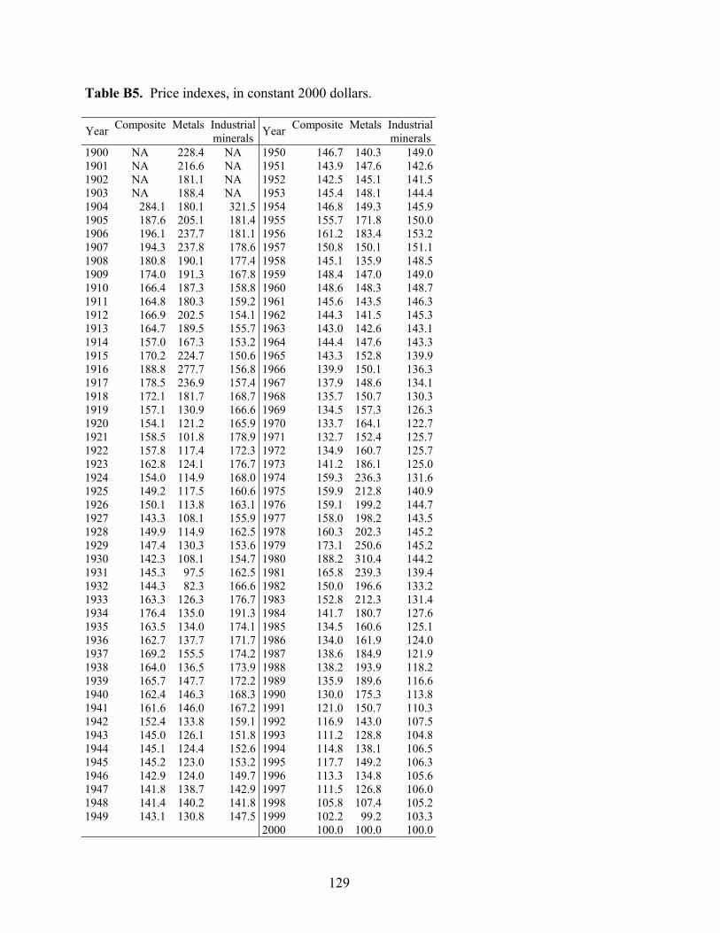
Table B5. Price indexes, in constant 2000 dollars.
Composite Metals Industrial Composite Metals IndustrialYear minerals Year minerals1900 NA 228.4 NA 1950 146.7 140.3 149.01901 NA 216.6 NA 1951 143.9 147.6 142.61902 NA 181.1 NA 1952 142.5 145.1 141.51903 NA 188.4 NA 1953 145.4 148.1 144.41904 284.1 180.1 321.5 1954 146.8 149.3 145.91905 187.6 205.1 181.4 1955 155.7 171.8 150.01906 196.1 237.7 181.1 1956 161.2 183.4 153.21907 194.3 237.8 178.6 1957 150.8 150.1 151.11908 180.8 190.1 177.4 1958 145.1 135.9 148.51909 174.0 191.3 167.8 1959 148.4 147.0 149.01910 166.4 187.3 158.8 1960 148.6 148.3 148.71911 164.8 180.3 159.2 1961 145.6 143.5 146.31912 166.9 202.5 154.1 1962 144.3 141.5 145.31913 164.7 189.5 155.7 1963 143.0 142.6 143.11914 157.0 167.3 153.2 1964 144.4 147.6 143.31915 170.2 224.7 150.6 1965 143.3 152.8 139.91916 188.8 277.7 156.8 1966 139.9 150.1 136.31917 178.5 236.9 157.4 1967 137.9 148.6 134.11918 172.1 181.7 168.7 1968 135.7 150.7 130.31919 157.1 130.9 166.6 1969 134.5 157.3 126.31920 154.1 121.2 165.9 1970 133.7 164.1 122.71921 158.5 101.8 178.9 1971 132.7 152.4 125.71922 157.8 117.4 172.3 1972 134.9 160.7 125.71923 162.8 124.1 176.7 1973 141.2 186.1 125.01924 154.0 114.9 168.0 1974 159.3 236.3 131.61925 149.2 117.5 160.6 1975 159.9 212.8 140.91926 150.1 113.8 163.1 1976 159.1 199.2 144.71927 143.3 108.1 155.9 1977 158.0 198.2 143.51928 149.9 114.9 162.5 1978 160.3 202.3 145.21929 147.4 130.3 153.6 1979 173.1 250.6 145.21930 142.3 108.1 154.7 1980 188.2 310.4 144.21931 145.3 97.5 162.5 1981 165.8 239.3 139.41932 144.3 82.3 166.6 1982 150.0 196.6 133.21933 163.3 126.3 176.7 1983 152.8 212.3 131.41934 176.4 135.0 191.3 1984 141.7 180.7 127.61935 163.5 134.0 174.1 1985 134.5 160.6 125.11936 162.7 137.7 171.7 1986 134.0 161.9 124.01937 169.2 155.5 174.2 1987 138.6 184.9 121.91938 164.0 136.5 173.9 1988 138.2 193.9 118.21939 165.7 147.7 172.2 1989 135.9 189.6 116.61940 162.4 146.3 168.3 1990 130.0 175.3 113.81941 161.6 146.0 167.2 1991 121.0 150.7 110.31942 152.4 133.8 159.1 1992 116.9 143.0 107.51943 145.0 126.1 151.8 1993 111.2 128.8 104.81944 145.1 124.4 152.6 1994 114.8 138.1 106.51945 145.2 123.0 153.2 1995 117.7 149.2 106.31946 142.9 124.0 149.7 1996 113.3 134.8 105.61947 141.8 138.7 142.9 1997 111.5 126.8 106.01948 141.4 140.2 141.8 1998 105.8 107.4 105.21949 143.1 130.8 147.5 1999 102.2 99.2 103.3
2000 100.0 100.0 100.0
129
Overall, the trend of the inflation-adjusted prices shown in the composite price index figure B1
decreased throughout the 20th century at an average annual rate of less than 1 percent for the
years 1905 to 2000. This downward trend occurred even though the use of mineral materials in
the United States increased during this time frame to meet the needs of the growing economy.
The declining long-term price trend is an indication that adequate sources of supply exist,
competition within the industry is prevalent, and the costs of production have decreased.
Figure B2 shows that industrial mineral commodity prices decreased during the 20th century.
Since industrial minerals account for two-thirds of the total value of mineral production included
in the U.S. economy, the pattern of this figure closely resembles figure B1, the index of
composite prices. Industrial minerals such as cement, crushed stone, and sand and gravel are
crucial to the U.S. construction industry.
Among the many reasons why raw construction mineral prices have declined were the advances
made in excavation and earth moving equipment. Initially, mining was done by hand. Steam
shovels were introduced in the early 20th century, which were soon after replaced by gasoline,
diesel, and electric powered equipment. There were also vast improvements in transportation
and other infrastructure during the century. These improvements allowed the industry to lower
costs that enabled them to reduce real prices and still operate at a profit.
130

0
50
100
150
200
250
1900 1910 1920 1930 1940 1950 1960 1970 1980 1990 2000
YEAR
U.S
. IND
UST
RIA
L M
INER
ALS
PRIC
E IN
DEX,
200
0 =
100
Index Linear trend
Figure B2. U.S. industrial minerals price index, in constant 2000 dollars, 1905-2000.
Cement accounts for more than 20 percent of the value of production of industrial minerals
included in the composite index and in the year 2000 was the industrial mineral with the second
largest value of nonfuel mineral production in the United States ($6,901 million), see table B1.
Most cement was used in the construction of bridges, buildings, highways, and other
infrastructure. The price history of cement is shown in figure B3. The trend line for the constant
dollar price of cement shows that, overall, the price declined during the 20th century. The real
price was above $110 per ton briefly at the beginning of the century, and again during the
“roaring twenties.” The lack of economic activity during the depression drove the price below
131
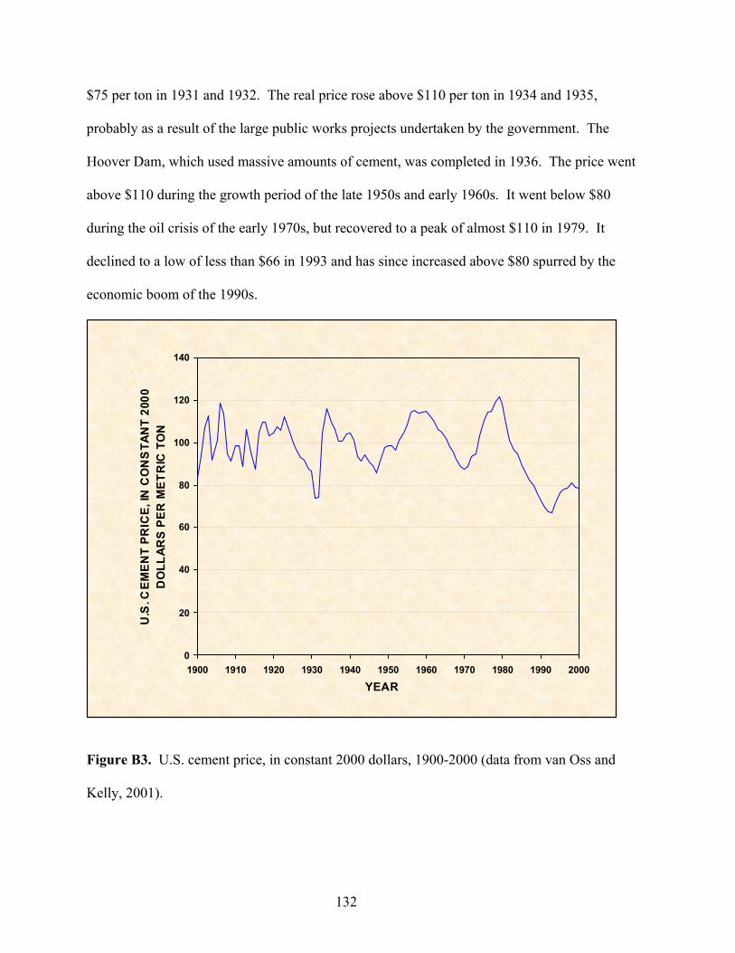
$75 per ton in 1931 and 1932. The real price rose above $110 per ton in 1934 and 1935,
probably as a result of the large public works projects undertaken by the government. The
Hoover Dam, which used massive amounts of cement, was completed in 1936. The price went
above $110 during the growth period of the late 1950s and early 1960s. It went below $80
during the oil crisis of the early 1970s, but recovered to a peak of almost $110 in 1979. It
declined to a low of less than $66 in 1993 and has since increased above $80 spurred by the
economic boom of the 1990s.
0
20
40
60
80
100
120
140
1900 1910 1920 1930 1940 1950 1960 1970 1980 1990 2000
YEAR
U.S
. CEM
ENT
PRIC
E, IN
CO
NS
TAN
T 20
00
DO
LLAR
S PE
R M
ETR
IC T
ON
Figure B3. U.S. cement price, in constant 2000 dollars, 1900-2000 (data from van Oss and
Kelly, 2001).
132
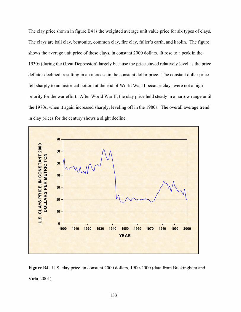
The clay price shown in figure B4 is the weighted average unit value price for six types of clays.
The clays are ball clay, bentonite, common clay, fire clay, fuller’s earth, and kaolin. The figure
shows the average unit price of these clays, in constant 2000 dollars. It rose to a peak in the
1930s (during the Great Depression) largely because the price stayed relatively level as the price
deflator declined, resulting in an increase in the constant dollar price. The constant dollar price
fell sharply to an historical bottom at the end of World War II because clays were not a high
priority for the war effort. After World War II, the clay price held steady in a narrow range until
the 1970s, when it again increased sharply, leveling off in the 1980s. The overall average trend
in clay prices for the century shows a slight decline.
0
10
20
30
40
50
60
70
1900 1910 1920 1930 1940 1950 1960 1970 1980 1990 2000
YEAR
U.S
. CLA
YS P
RIC
E, IN
CO
NS
TAN
T 20
00
DO
LLA
RS
PER
MET
RIC
TO
N
Figure B4. U.S. clay price, in constant 2000 dollars, 1900-2000 (data from Buckingham and
Virta, 2001).
133
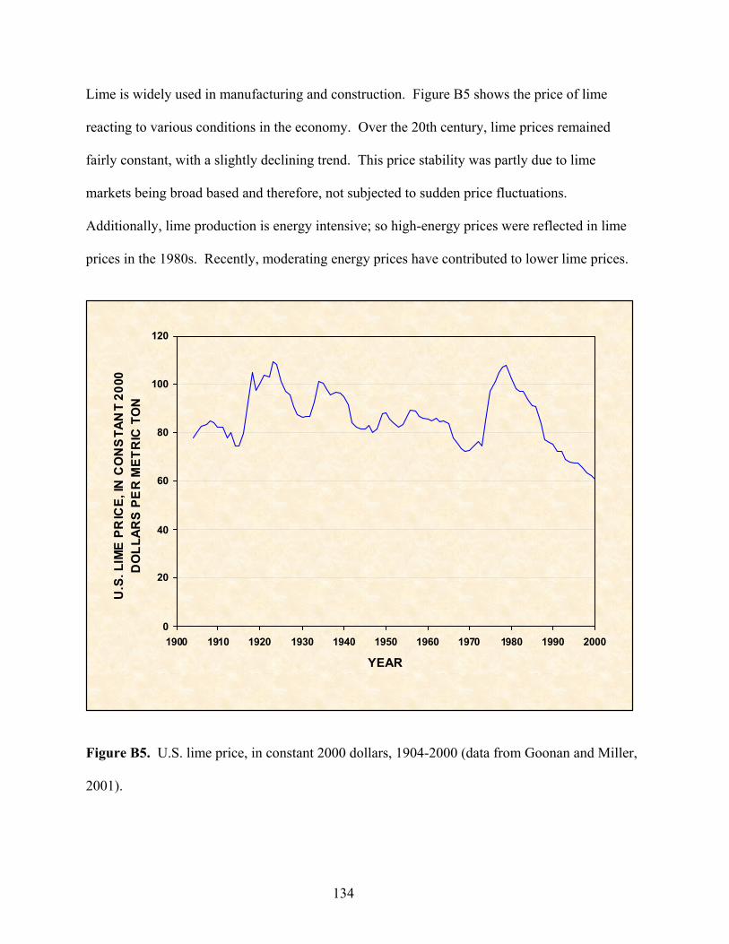
Lime is widely used in manufacturing and construction. Figure B5 shows the price of lime
reacting to various conditions in the economy. Over the 20th century, lime prices remained
fairly constant, with a slightly declining trend. This price stability was partly due to lime
markets being broad based and therefore, not subjected to sudden price fluctuations.
Additionally, lime production is energy intensive; so high-energy prices were reflected in lime
prices in the 1980s. Recently, moderating energy prices have contributed to lower lime prices.
0
20
40
60
80
100
120
1900 1910 1920 1930 1940 1950 1960 1970 1980 1990 2000
YEAR
U.S
. LIM
E P
RIC
E, IN
CO
NS
TAN
T 20
00
DO
LLAR
S P
ER
MET
RIC
TO
N
Figure B5. U.S. lime price, in constant 2000 dollars, 1904-2000 (data from Goonan and Miller,
2001).
134
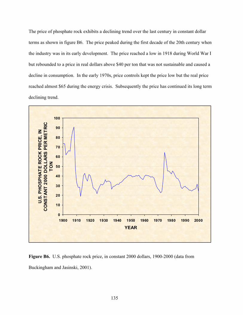
The price of phosphate rock exhibits a declining trend over the last century in constant dollar
terms as shown in figure B6. The price peaked during the first decade of the 20th century when
the industry was in its early development. The price reached a low in 1918 during World War I
but rebounded to a price in real dollars above $40 per ton that was not sustainable and caused a
decline in consumption. In the early 1970s, price controls kept the price low but the real price
reached almost $65 during the energy crisis. Subsequently the price has continued its long term
declining trend.
0
10
20
30
40
50
60
70
80
90
100
1900 1910 1920 1930 1940 1950 1960 1970 1980 1990 2000
YEAR
U.S.
PHO
SPHA
TE R
OC
K P
RICE
, IN
CO
NSTA
NT 2
000
DO
LLAR
S PE
R M
ETRI
C
TON
Figure B6. U.S. phosphate rock price, in constant 2000 dollars, 1900-2000 (data from
Buckingham and Jasinski, 2001).
135
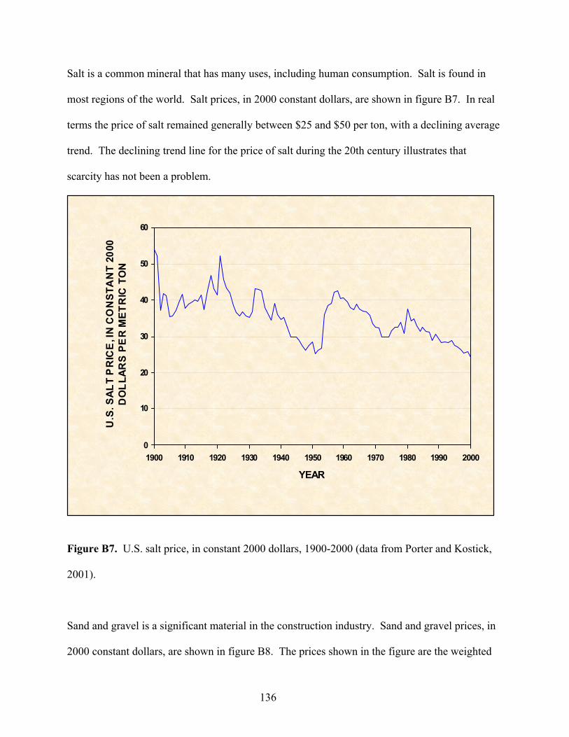
Salt is a common mineral that has many uses, including human consumption. Salt is found in
most regions of the world. Salt prices, in 2000 constant dollars, are shown in figure B7. In real
terms the price of salt remained generally between $25 and $50 per ton, with a declining average
trend. The declining trend line for the price of salt during the 20th century illustrates that
scarcity has not been a problem.
0
10
20
30
40
50
60
1900 1910 1920 1930 1940 1950 1960 1970 1980 1990 2000
YEAR
U.S
. SAL
T P
RIC
E, I
N C
ON
STA
NT
2000
D
OLL
ARS
PE
R M
ETR
IC T
ON
Figure B7. U.S. salt price, in constant 2000 dollars, 1900-2000 (data from Porter and Kostick,
2001).
Sand and gravel is a significant material in the construction industry. Sand and gravel prices, in
2000 constant dollars, are shown in figure B8. The prices shown in the figure are the weighted
136
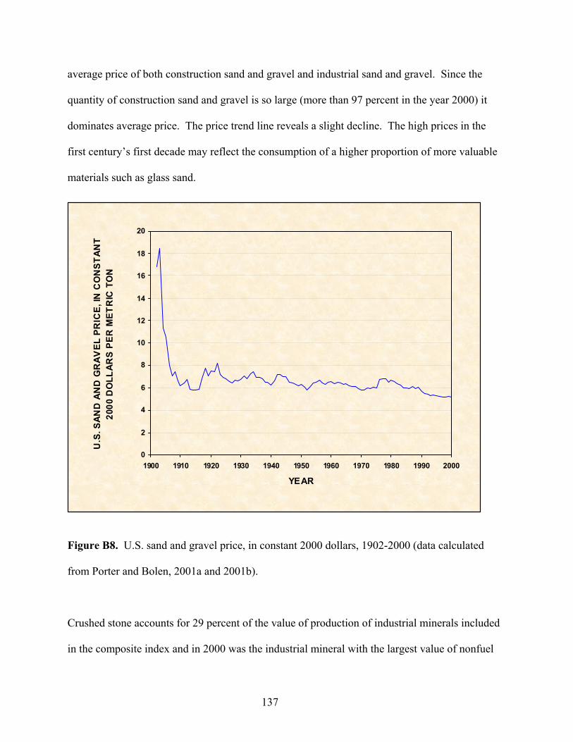
average price of both construction sand and gravel and industrial sand and gravel. Since the
quantity of construction sand and gravel is so large (more than 97 percent in the year 2000) it
dominates average price. The price trend line reveals a slight decline. The high prices in the
first century’s first decade may reflect the consumption of a higher proportion of more valuable
materials such as glass sand.
0
2
4
6
8
10
12
14
16
18
20
1900 1910 1920 1930 1940 1950 1960 1970 1980 1990 2000
YEAR
U.S
. SAN
D A
ND
GR
AVEL
PR
ICE,
IN C
ON
STAN
T 20
00 D
OLL
ARS
PER
MET
RIC
TO
N
Figure B8. U.S. sand and gravel price, in constant 2000 dollars, 1902-2000 (data calculated
from Porter and Bolen, 2001a and 2001b).
Crushed stone accounts for 29 percent of the value of production of industrial minerals included
in the composite index and in 2000 was the industrial mineral with the largest value of nonfuel
137
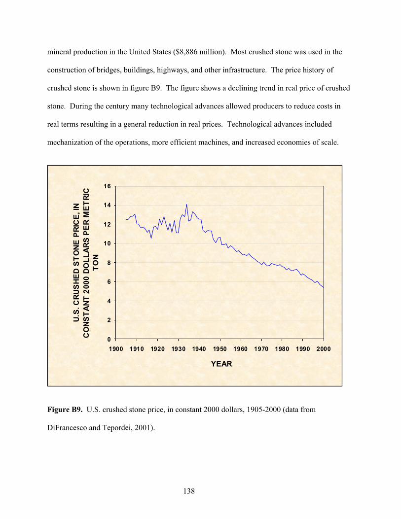
mineral production in the United States ($8,886 million). Most crushed stone was used in the
construction of bridges, buildings, highways, and other infrastructure. The price history of
crushed stone is shown in figure B9. The figure shows a declining trend in real price of crushed
stone. During the century many technological advances allowed producers to reduce costs in
real terms resulting in a general reduction in real prices. Technological advances included
mechanization of the operations, more efficient machines, and increased economies of scale.
0
2
4
6
8
10
12
14
16
1900 1910 1920 1930 1940 1950 1960 1970 1980 1990 2000
YEAR
U.S.
CRU
SHED
STO
NE P
RIC
E, IN
C
ONS
TANT
200
0 DO
LLAR
S PE
R M
ETRI
C
TON
Figure B9. U.S. crushed stone price, in constant 2000 dollars, 1905-2000 (data from
DiFrancesco and Tepordei, 2001).
138
The metals price index has shown more volatility than the industrial minerals price index
throughout the century (figure B10). This may be because the metals markets are made up of a
smaller number of large producers and consumers and the industrial minerals markets generally
have a larger number of smaller producers and consumers. Copper, lead, and zinc, which
comprise 45 percent of the index, have downward trends. However, the trends for gold and iron
ore prices, which comprise the remainder of the index, were up slightly15. When data for the five
metals are combined into the metal price index, it has a slight downward trend. The index has a
large peak in 1916, which is probably related to high demand during World War I. Another
significant peak in 1980 can be attributed to speculation in gold. Data in current and constant
dollar terms for the individual metal commodities can be found in Tables B2 and B3. A
discussion of the price trends for each of the commodities included in the metals price index, and
aluminum, follows.
15 Even though the long-term trends for gold and iron ore were up slightly, the year 2000 constant dollar price for both metals was less than their respective constant dollar prices in the year 1900.
139
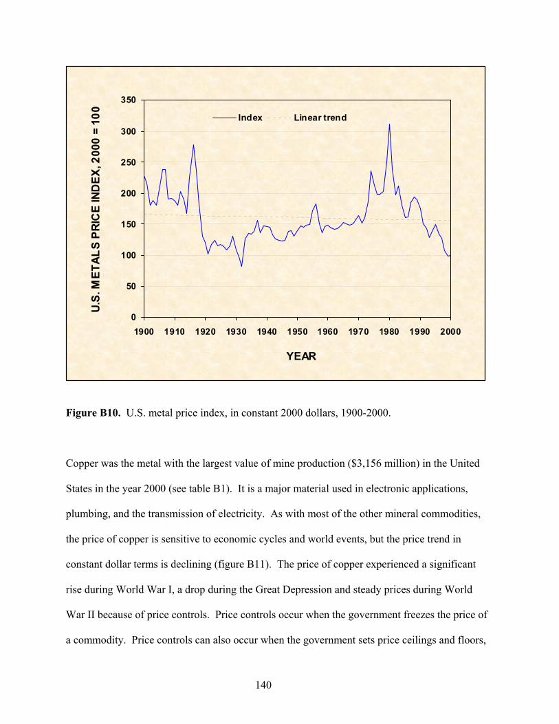
0
50
100
150
200
250
300
350
1900 1910 1920 1930 1940 1950 1960 1970 1980 1990 2000
YEAR
U.S.
MET
ALS
PRIC
E IN
DEX
, 200
0 =
100
Index Linear trend
Figure B10. U.S. metal price index, in constant 2000 dollars, 1900-2000.
Copper was the metal with the largest value of mine production ($3,156 million) in the United
States in the year 2000 (see table B1). It is a major material used in electronic applications,
plumbing, and the transmission of electricity. As with most of the other mineral commodities,
the price of copper is sensitive to economic cycles and world events, but the price trend in
constant dollar terms is declining (figure B11). The price of copper experienced a significant
rise during World War I, a drop during the Great Depression and steady prices during World
War II because of price controls. Price controls occur when the government freezes the price of
a commodity. Price controls can also occur when the government sets price ceilings and floors,
140
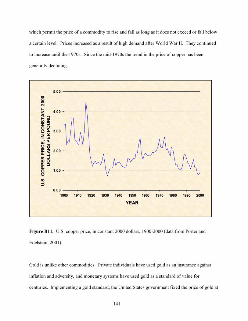
which permit the price of a commodity to rise and fall as long as it does not exceed or fall below
a certain level. Prices increased as a result of high demand after World War II. They continued
to increase until the 1970s. Since the mid-1970s the trend in the price of copper has been
generally declining.
0.00
1.00
2.00
3.00
4.00
5.00
1900 1910 1920 1930 1940 1950 1960 1970 1980 1990 2000
YEAR
U.S.
CO
PPER
PRI
CE,
IN C
ONS
TANT
200
0 D
OLL
ARS
PER
POUN
D
Figure B11. U.S. copper price, in constant 2000 dollars, 1900-2000 (data from Porter and
Edelstein, 2001).
Gold is unlike other commodities. Private individuals have used gold as an insurance against
inflation and adversity, and monetary systems have used gold as a standard of value for
centuries. Implementing a gold standard, the United States government fixed the price of gold at
141
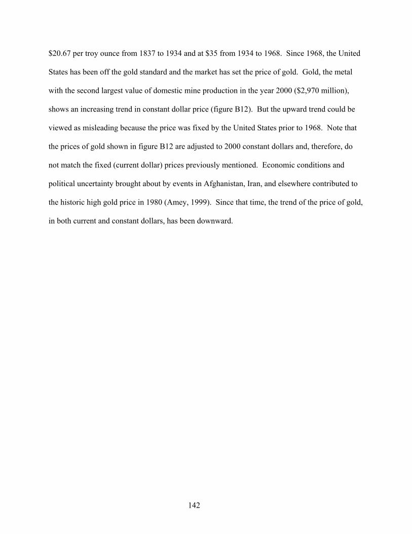
$20.67 per troy ounce from 1837 to 1934 and at $35 from 1934 to 1968. Since 1968, the United
States has been off the gold standard and the market has set the price of gold. Gold, the metal
with the second largest value of domestic mine production in the year 2000 ($2,970 million),
shows an increasing trend in constant dollar price (figure B12). But the upward trend could be
viewed as misleading because the price was fixed by the United States prior to 1968. Note that
the prices of gold shown in figure B12 are adjusted to 2000 constant dollars and, therefore, do
not match the fixed (current dollar) prices previously mentioned. Economic conditions and
political uncertainty brought about by events in Afghanistan, Iran, and elsewhere contributed to
the historic high gold price in 1980 (Amey, 1999). Since that time, the trend of the price of gold,
in both current and constant dollars, has been downward.
142
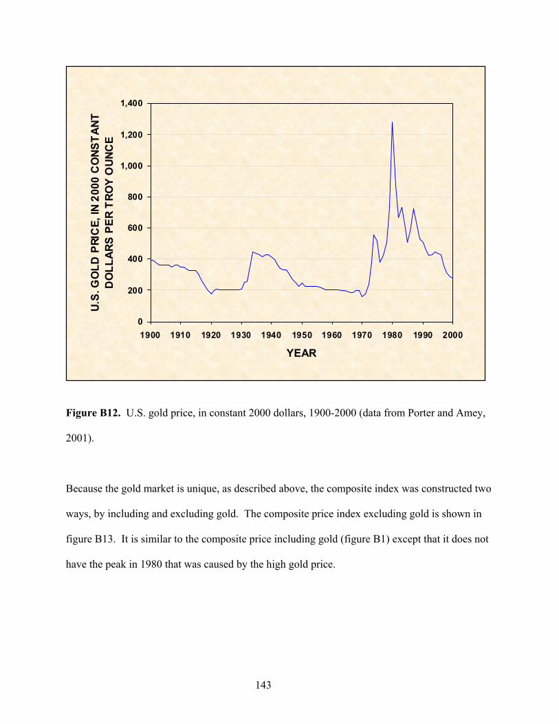
0
200
400
600
800
1,000
1,200
1,400
1900 1910 1920 1930 1940 1950 1960 1970 1980 1990 2000
YEAR
U.S.
GO
LD P
RIC
E, IN
200
0 C
ONS
TANT
D
OLL
ARS
PER
TRO
Y O
UNC
E
Figure B12. U.S. gold price, in constant 2000 dollars, 1900-2000 (data from Porter and Amey,
2001).
Because the gold market is unique, as described above, the composite index was constructed two
ways, by including and excluding gold. The composite price index excluding gold is shown in
figure B13. It is similar to the composite price including gold (figure B1) except that it does not
have the peak in 1980 that was caused by the high gold price.
143
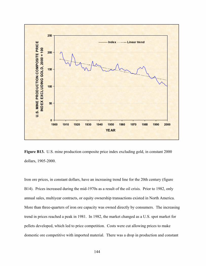
0
50
100
150
200
250
1900 1910 1920 1930 1940 1950 1960 1970 1980 1990 2000
YEAR
U.S
. MIN
E P
RO
DU
CTI
ON
CO
MPO
SITE
PR
ICE
IND
EX E
XCLU
DIN
G G
OLD
, 200
0 =
100
Index Linear trend
Figure B13. U.S. mine production composite price index excluding gold, in constant 2000
dollars, 1905-2000.
Iron ore prices, in constant dollars, have an increasing trend line for the 20th century (figure
B14). Prices increased during the mid-1970s as a result of the oil crisis. Prior to 1982, only
annual sales, multiyear contracts, or equity ownership transactions existed in North America.
More than three-quarters of iron ore capacity was owned directly by consumers. The increasing
trend in prices reached a peak in 1981. In 1982, the market changed as a U.S. spot market for
pellets developed, which led to price competition. Costs were cut allowing prices to make
domestic ore competitive with imported material. There was a drop in production and constant
144

dollar prices declined. By the mid-1980s, iron ore prices declined to pre-World War II levels in
terms of constant dollars (Kirk, 1999).
0
10
20
30
40
50
60
70
80
90
1900 1910 1920 1930 1940 1950 1960 1970 1980 1990 2000
YEAR
U.S.
IRO
N O
RE
PRIC
E, IN
CO
NSTA
NT 2
000
DO
LLAR
S PE
R M
ETR
IC T
ON
Figure B14. U.S. iron ore price, in constant 2000 dollars, 1900-2000 (data from Kelly and Kirk,
2001).
The price of lead has a declining trend for the century in spite of many peaks and valleys through
the period (figure B15). Increased demand for the war effort produced a peak during World War
I. Demand generated by the booming of the economy produced another one in the 1920s. Lack
of demand resulting from the collapse in the economy resulted in a price drop during the Great
Depression. Prices were controlled during World War II, but the increased demand during the
145
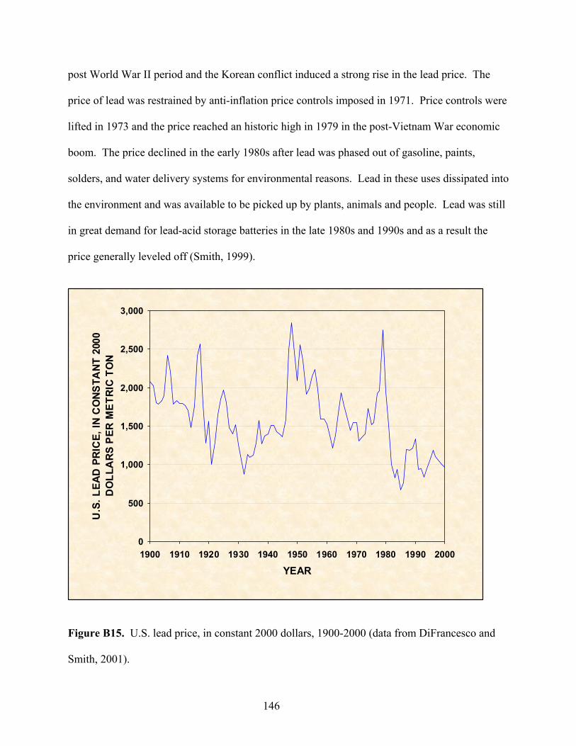
post World War II period and the Korean conflict induced a strong rise in the lead price. The
price of lead was restrained by anti-inflation price controls imposed in 1971. Price controls were
lifted in 1973 and the price reached an historic high in 1979 in the post-Vietnam War economic
boom. The price declined in the early 1980s after lead was phased out of gasoline, paints,
solders, and water delivery systems for environmental reasons. Lead in these uses dissipated into
the environment and was available to be picked up by plants, animals and people. Lead was still
in great demand for lead-acid storage batteries in the late 1980s and 1990s and as a result the
price generally leveled off (Smith, 1999).
0
500
1,000
1,500
2,000
2,500
3,000
1900 1910 1920 1930 1940 1950 1960 1970 1980 1990 2000
YEAR
U.S
. LEA
D P
RIC
E, IN
CO
NSTA
NT 2
000
DO
LLA
RS P
ER M
ETRI
C TO
N
Figure B15. U.S. lead price, in constant 2000 dollars, 1900-2000 (data from DiFrancesco and
Smith, 2001).
146
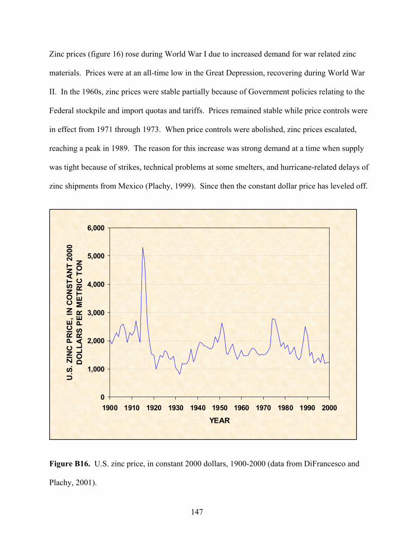
Zinc prices (figure 16) rose during World War I due to increased demand for war related zinc
materials. Prices were at an all-time low in the Great Depression, recovering during World War
II. In the 1960s, zinc prices were stable partially because of Government policies relating to the
Federal stockpile and import quotas and tariffs. Prices remained stable while price controls were
in effect from 1971 through 1973. When price controls were abolished, zinc prices escalated,
reaching a peak in 1989. The reason for this increase was strong demand at a time when supply
was tight because of strikes, technical problems at some smelters, and hurricane-related delays of
zinc shipments from Mexico (Plachy, 1999). Since then the constant dollar price has leveled off.
0
1,000
2,000
3,000
4,000
5,000
6,000
1900 1910 1920 1930 1940 1950 1960 1970 1980 1990 2000
YEAR
U.S
. ZIN
C PR
ICE,
IN C
ON
STAN
T 20
00
DO
LLA
RS P
ER M
ETRI
C TO
N
Figure B16. U.S. zinc price, in constant 2000 dollars, 1900-2000 (data from DiFrancesco and
Plachy, 2001).
147
Aluminum is not a component of the U.S. price indexes because U.S. production of bauxite
provides less than 1 percent of the U.S. requirement. The small amount of bauxite produced
domestically is not used to produce aluminum metal, but is used for abrasives, chemicals, and
refractories. The aluminum industry is however a major industry in the United States, as it
imports bauxite ore, or alumina, and processes it into aluminum. In the year 2000, production
was valued at over $6 billion (Buckingham and Plunkert, 2001). Therefore, it is important to
briefly discuss the trend of aluminum prices as shown in figure B17.
Before World War I, the price of aluminum was elevated because the production process was in
its infancy and supply was limited. A historic high was reached in World War I because of high
demand for use in military aircraft. With the advent of new and improved technology that
reduced production costs and the development of a global market, the price of aluminum
declined similarly to other mineral commodities.
148
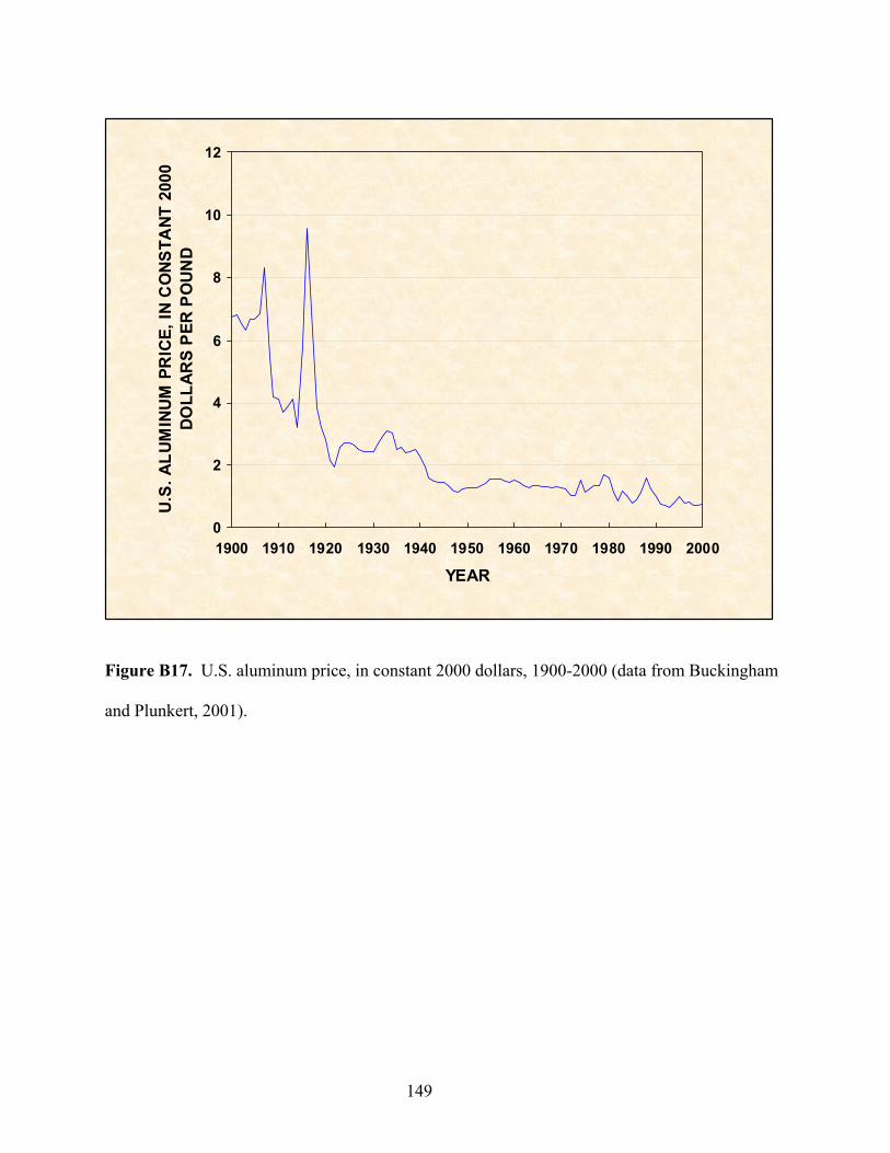
0
2
4
6
8
10
12
1900 1910 1920 1930 1940 1950 1960 1970 1980 1990 2000
YEAR
U.S.
ALU
MIN
UM P
RIC
E, IN
CO
NSTA
NT 2
000
DOLL
ARS
PER
POUN
D
Figure B17. U.S. aluminum price, in constant 2000 dollars, 1900-2000 (data from Buckingham
and Plunkert, 2001).
149
References
Amey, E.B., 1999, Gold, in Metal prices in the United States through 1998: U.S. Geological Survey, p. 49-53. Buckingham, D.A., and Jasinski, S.M., 2001, Phosphate rock statistics, in Historical statistics for mineral commodities in the United States: U.S. Geological Survey Open-File Report 01-006. Buckingham, D.A., and Plunkert, P.A., 2001, Aluminum statistics, in Historical statistics for mineral commodities in the United States: U.S. Geological Survey Open-File Report 01-006. Buckingham, D.A., and Virta, R.L., 2001, Clay statistics, in Historical statistics for mineral commodities in the United States: U.S. Geological Survey Open-File Report 01-006. DiFrancesco, C.A., and Plachy, Jozef, 2001, Zinc statistics, in Historical statistics for mineral commodities in the United States: U.S. Geological Survey Open-File Report 01-006.
Porter, K.E., and Amey, E.B., 2001, Gold statistics, in Historical statistics for mineral commodities in the United States: U.S. Geological Survey Open-File Report 01-006.
DiFrancesco, C.A., and Smith, G.R., 2001, Lead statistics, in Historical statistics for mineral commodities in the United States: U.S. Geological Survey Open-File Report 01-006. DiFrancesco, C.A., and Tepordei, V.V., 2001, Stone (crushed) statistics, in Historical statistics for mineral commodities in the United States: U.S. Geological Survey Open-File Report 01-006. Goonan, T.G., and Miller, M.M., 2001, Lime statistics, in Historical statistics for mineral commodities in the United States: U.S. Geological Survey Open-File Report 01-006. Kelly, T.D., and Kirk, D.L., 2001, Iron ore statistics, in Historical statistics for mineral commodities in the United States: U.S. Geological Survey Open-File Report 01-006. Kirk, W.S., 1999, Iron ore, in Metal prices in the United States through 1998: U.S. Geological Survey, p. 69-72. Mansfield, Edwin, 1987, Statistics for business and economics, methods and applications, 3rd edition: New York, W.W. Norton & Company, 698 p. Plachy, Jozef, 1999, Zinc, in Metal prices in the United States through 1998: U.S. Geological Survey, p. 171-173.
Porter, K.E., and Bolen, W.P., 2001a, Sand and gravel (construction) statistics, in Historical statistics for mineral commodities in the United States: U.S. Geological Survey Open-File Report 01-006.
150
Porter, K.E., and Bolen, W.P., 2001b, Sand and gravel (industrial) statistics, in Historical statistics for mineral commodities in the United States: U.S. Geological Survey Open-File Report 01-006. Porter, K.E., and Edelstein, D.L., 2001, Copper statistics, in Historical statistics for mineral commodities in the United States: U.S. Geological Survey Open-File Report 01-006. Porter, K.E., and Kostick, D.S., 2001, Salt statistics, in Historical statistics for mineral commodities in the United States: U.S. Geological Survey Open-File Report 01-006. Smith, G.R., 1999, Lead, in Metal prices in the United States through 1998: U.S. Geological Survey, p. 73-75. Smith, S.D., 2002, Statistical summary, in Metals and Minerals: U.S. Geological Survey Minerals Yearbook 2000, v. I, p. 3.1-3.29. U.S. Census Bureau, 1975, Historical statistics of the United States– Colonial times to 1970: U.S. Census Bureau series E 135, v. I, p. 210-211.
U.S. Geological Survey, 2001, Historical statistics for mineral commodities in the United States: U.S. Geological Survey Open-File Report 01-006. van Oss, H.G., and Kelly, T.D., 2001, Cement statistics, in Historical statistics for mineral commodities in the United States: U.S. Geological Survey Open-File Report 01-006.
Internet references cited U.S. Department of Labor, Bureau of Labor Statistics, 2001, Consumer price indexes, accessed December 18, 2001 at URL ftp://ftp.bls.gov/pub/special.requests/cpi/cpiai.txt.
151
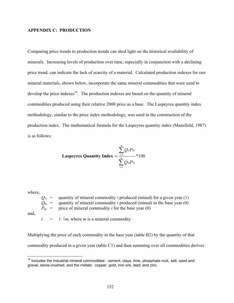
APPENDIX C: PRODUCTION
Comparing price trends to production trends can shed light on the historical availability of
minerals. Increasing levels of production over time, especially in conjunction with a declining
price trend, can indicate the lack of scarcity of a material. Calculated production indexes for raw
mineral materials, shown below, incorporate the same mineral commodities that were used to
develop the price indexes16. The production indexes are based on the quantity of mineral
commodities produced using their relative 2000 price as a base. The Laspeyres quantity index
methodology, similar to the price index methodology, was used in the construction of the
production index. The mathematical formula for the Laspeyres quantity index (Mansfield, 1987)
is as follows:
Laspeyres Quantity Index 100*
100
101
∑
∑
=
== m
iii
m
iii
PQ
PQ
where,
Q1i = quantity of mineral commodity i produced (mined) for a given year (1) Q0i = quantity of mineral commodity i produced (mined) in the base year (0) P0i = price of mineral commodity i for the base year (0)
and, i = 1 m, where m is a mineral commodity
Multiplying the price of each commodity in the base year (table B2) by the quantity of that
commodity produced in a given year (table C1) and then summing over all commodities derives
16 Includes the industrial mineral commodities: cement, clays, lime, phosphate rock, salt, sand and gravel, stone-crushed, and the metals: copper, gold, iron ore, lead, and zinc.
152
the value in the given year using base year prices. This sum is the numerator of the equation.
Multiplying the price of each commodity in the base year by the quantity produced in the base
year and then summing over all commodities derives the value of mineral production for these
commodities in the base year. This sum is the denominator of the equation. The result of the
division of the numerator by the denominator is an index that reflects relative changes in the
quantity produced for all of the included commodities with the weight of each commodity
determined by its price in the base year (table C2).
153
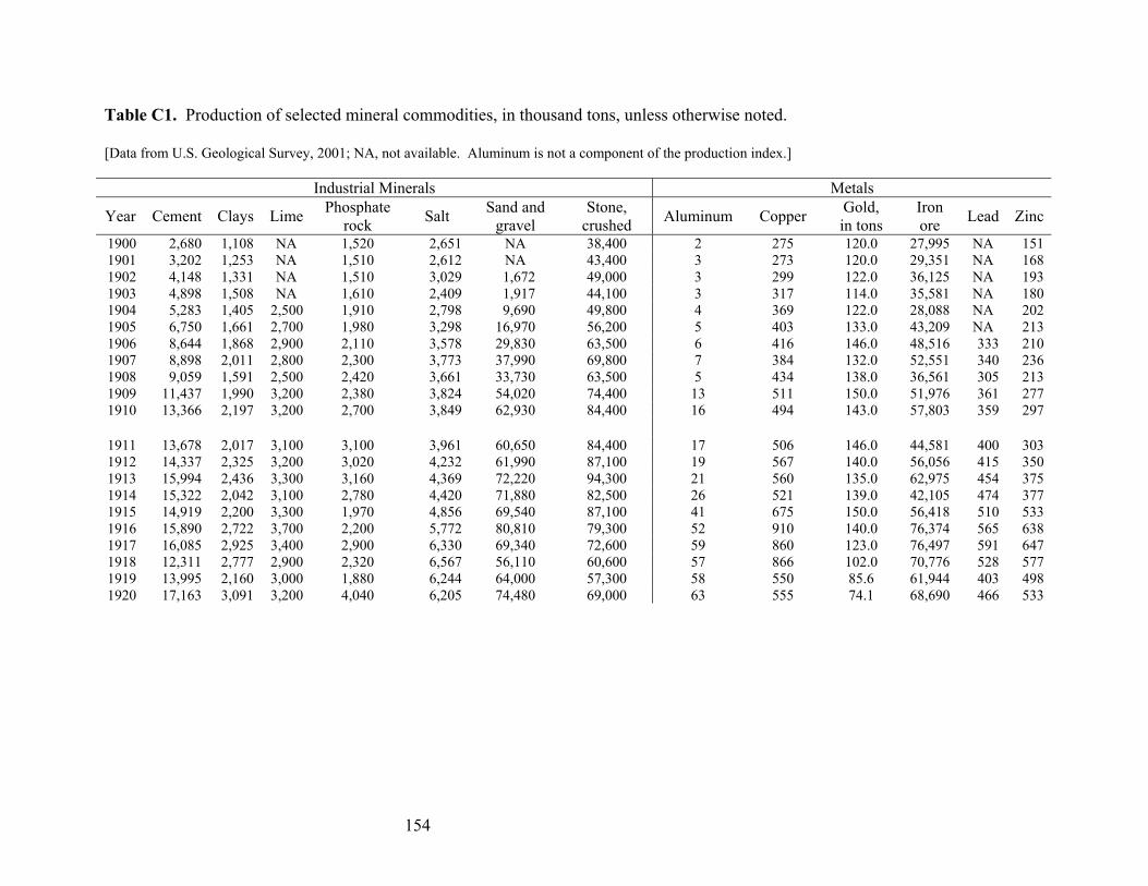
Table C1. Production of selected mineral commodities, in thousand tons, unless otherwise noted. [Data from U.S. Geological Survey, 2001; NA, not available. Aluminum is not a component of the production index.]
Industrial Minerals Metals
Year Salt Cement Clays Lime Phosphate rock
Sand and gravel
Stone, crushed Aluminum Copper Gold,
in tons Iron ore Lead Zinc
1900 0 2,680 1,108 NA 1,52 2,651 NA 38,400 2 275 120.0 27,995 NA 1511901 1,510 3,202 1,253 NA 2,612 NA 43,400 3 273 120.0 29,351 NA 1681902 1,510 1 2 4,148 1,331 NA 3,029 ,67 49,000 3 299 122.0 36,125 NA 193 1903 4, 8 8 1,610 89 1,50 NA 2,409 1,917 44,100 3 317 114.0 35,581 NA 180 1904 5,283 1,405 2,500 1,910 2,798 9,690 49,800 4 369 122.0 28,088 NA 202 1905 1,980 6,750 1,661 2,700 3,298 16,970 56,200 5 403 133.0 43,209 NA 2131906 2,110 8,644 1,868 2,900 3,578 29,830 63,500 6 416 146.0 48,516 333 2101907 8,898 2,011 2,800 2,300 3,773 37,990 69,800 7 384 132.0 52,551 340 2361908 9,059 1,591 2,500 2,420 3,661 33,730 63,500 5 434 138.0 36,561 305 2131909 11,437 1,990 3,200 2,380 3,824 54,020 74,400 13 511 150.0 51,976 361 2771910 13,366 2,197 3,200 2,700 3,849 62,930 84,400 16 494 143.0 57,803 359 297
1911 3, 0 13,678 2,017 3,100 10 3,961 60,650 84,400 17 506 146.0 44,581 400 3031912 3,020 7 14,337 2,325 3,200 4,232 61,990 87,100 19 56 140.0 56,056 415 3501913 15,994 2,436 3,300 3,160 4,369 72,220 94,300 21 560 135.0 62,975 454 3751914 15,322 2,042 3,100 2,780 4,420 71,880 82,500 26 521 139.0 42,105 474 3771915 14,919 2,200 3,300 1,970 4,856 69,540 87,100 41 675 150.0 56,418 510 5331916 15,890 2,722 3,700 2,200 5,772 80,810 79,300 52 910 140.0 76,374 565 6381917 16,085 2,925 3,400 2,900 6,330 69,340 72,600 59 860 123.0 76,497 591 6471918 12,311 2,777 2,900 2,320 6,567 56,110 60,600 57 866 102.0 70,776 528 5771919 13,995 2,160 3,000 1,880 6,244 64,000 57,300 58 550 85.6 61,944 403 4981920 17,163 3,091 3,200 4,040 6,205 74,480 69,000 63 555 74.1 68,690 466 533
154
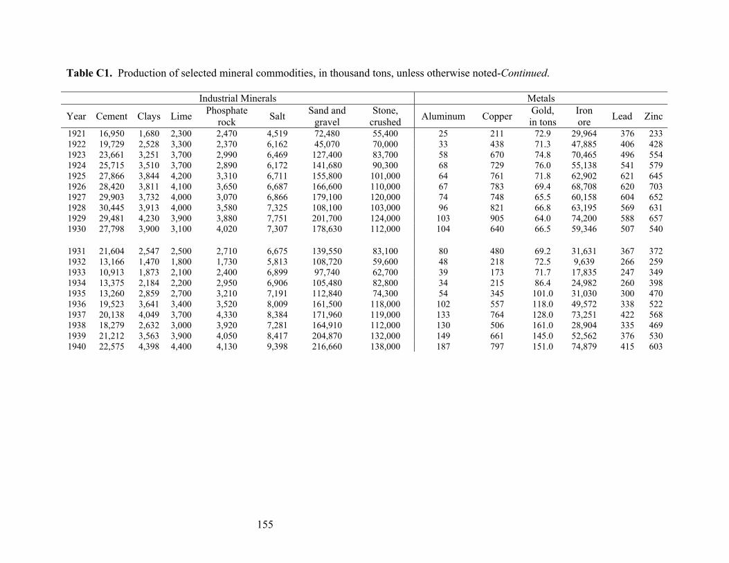
Table C1. Production of selected mineral commodities, in thousand tons, unless otherwise noted-Continued.
Industrial Minerals Metals
Year Cement Clays Lime Phosphate rock Salt Sand and
gravel Stone,
crushed Aluminum Copper Gold, in tons
Iron ore Lead Zinc
1921 16,950 1,680 2,300 2,470 4,519 72,480 55,400 25 211 72.9 29,964 376 2331922 0 19,729 2,528 3,300 2,37 6,162 45,070 70,000 33 438 71.3 47,885 406 4281923 23,661 3,251 3,700 2,990 6,469 127,400 83,700 58 670 74.8 70,465 496 5541924 25,715 3,510 3,700 2,890 6,172 141,680 90,300 68 729 76.0 55,138 541 5791925 0 27,866 3,844 4,200 3,31 6,711 155,800 101,000 64 761 71.8 62,902 621 6451926 3,650 28,420 3,811 4,100 6,687 166,600 110,000 67 783 69.4 68,708 620 7031927 29,903 3,732 4,000 3,070 6,866 179,100 120,000 74 748 65.5 60,158 604 6521928 0 30,445 3,913 4,000 3,58 7,325 108,100 103,000 96 821 66.8 63,195 569 6311929 29,481 4,230 3,900 3,880 7,751 201,700 124,000 103 905 64.0 74,200 588 6571930 0 27,798 3,900 3,100 4,02 7,307 178,630 112,000 104 640 66.5 59,346 507 540
1931 21,604 2,547 2,500 2,710 6,675 139,550 83,100 80 480 69.2 31,631 367 3721932 13,166 1,470 1,800 0 1,73 5,813 108,720 59,600 48 218 72.5 9,639 266 2591933 10,913 1,873 2,100 2,400 6,899 97,740 62,700 39 173 71.7 17,835 247 3491934 13,375 2,184 2,200 2,950 6,906 105,480 82,800 34 215 86.4 24,982 260 3981935 13,260 2,859 2,700 3,210 7,191 112,840 74,300 54 345 101.0 31,030 300 4701936 19,523 3,641 3,400 3,520 8,009 161,500 118,000 102 557 118.0 49,572 338 5221937 20,138 4,049 3,700 4,330 8,384 171,960 119,000 133 764 128.0 73,251 422 5681938 18,279 2,632 3,000 3,920 7,281 164,910 112,000 130 506 161.0 28,904 335 4691939 21,212 3,563 3,900 4,050 8,417 204,870 132,000 149 661 145.0 52,562 376 5301940 22,575 4,398 4,400 4,130 9,398 216,660 138,000 187 797 151.0 74,879 415 603
155
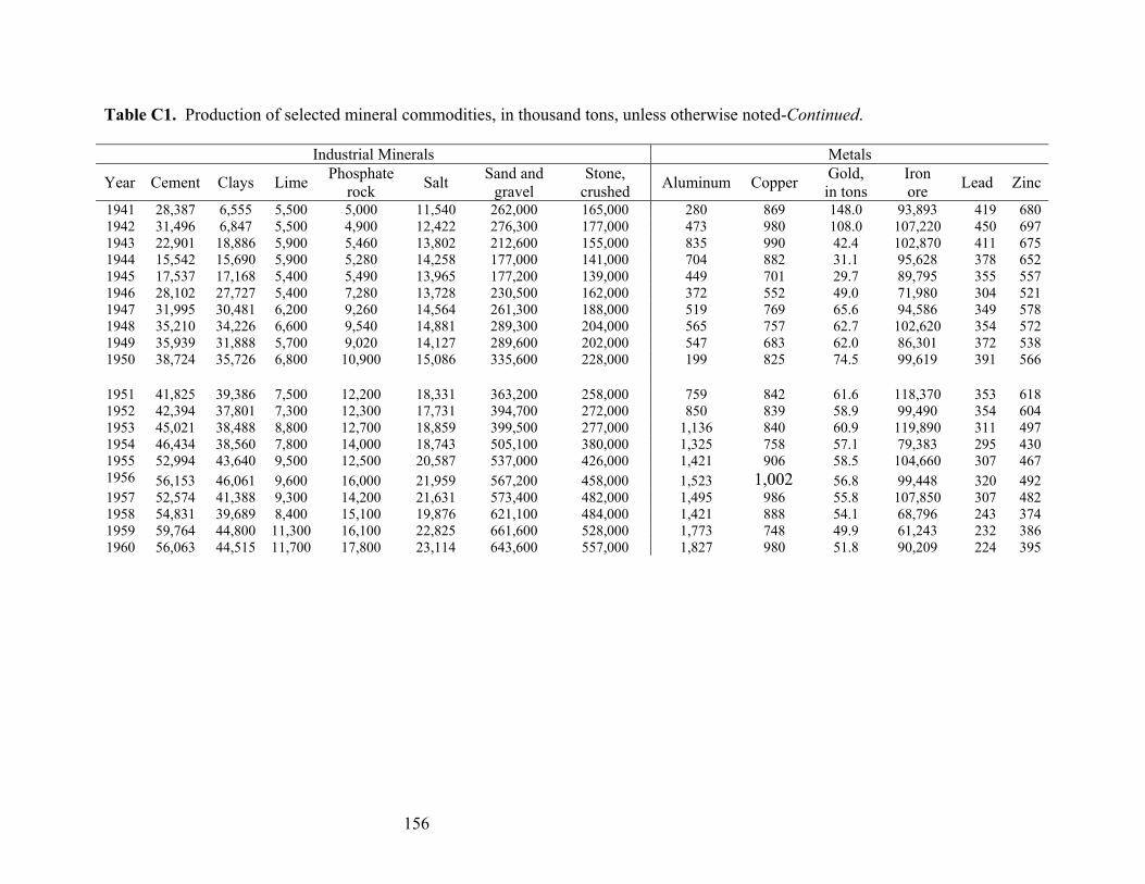
Table C1. Production of selected mineral commodities, in thousand tons, unless otherwise noted-Continued.
Industrial Minerals Metals
Year Cement Clays Lime Phosphate rock Salt Sand and
gravel Stone,
crushed Aluminum Copper Gold, in tons
Iron ore Lead Zinc
1941 28,387 6,555 5,500 5,000 11,540 262,000 165,000 280 869 148.0 93,893 419 6801942 31,496 6,847 5,500 4,900 12,422 276,300 177,000 473 980 108.0 107,220 450 6971943 22,901 18,886 5,900 5,460 13,802 212,600 155,000 835 990 42.4 102,870 411 6751944 15,542 15,690 5,900 5,280 14,258 177,000 141,000 704 882 31.1 95,628 378 6521945 1 1 7,537 7,168 5,400 5,490 13,965 177,200 139,000 449 701 29.7 89,795 355 5571946 28,102 27,727 5,400 7,280 13,728 230,500 162,000 372 552 49.0 71,980 304 5211947 31,995 30,481 6,200 9,260 14,564 261,300 188,000 519 769 65.6 94,586 349 5781948 35,210 34,226 6,600 9,540 14,881 289,300 204,000 565 757 62.7 102,620 354 5721949 35,939 31,888 5,700 9,020 14,127 289,600 202,000 547 683 62.0 86,301 372 5381950 38,724 35,726 6,800 10,900 15,086 335,600 228,000 199 825 74.5 99,619 391 566
1951 41,825 39,386 7,500 12,200 18,331 363,200 258,000 759 842 61.6 118,370 353 6181952 42,394 37,801 7,300 12,300 17,731 394,700 272,000 850 839 58.9 99,490 354 6041953 45,021 38,488 8,800 12,700 18,859 399,500 277,000 1,136 840 60.9 119,890 311 4971954 46,434 38,560 7,800 14,000 18,743 505,100 380,000 1,325 758 57.1 79,383 295 4301955 52,994 43,640 9,500 12,500 20,587 537,000 426,000 1,421 906 58.5 104,660 307 4671956 56,153 46,061 9,600 16,000 21,959 567,200 458,000 1,523 1,002 56.8 99,448 320 4921957 52,574 41,388 9,300 14,200 21,631 573,400 482,000 1,495 986 55.8 107,850 307 4821958 54,831 39,689 8,400 15,100 19,876 621,100 484,000 1,421 888 54.1 68,796 243 3741959 59,764 44,800 11,300 16,100 22,825 661,600 528,000 1,773 748 49.9 61,243 232 3861960 56,063 44,515 11,700 17,800 23,114 643,600 557,000 1,827 980 51.8 90,209 224 395
156
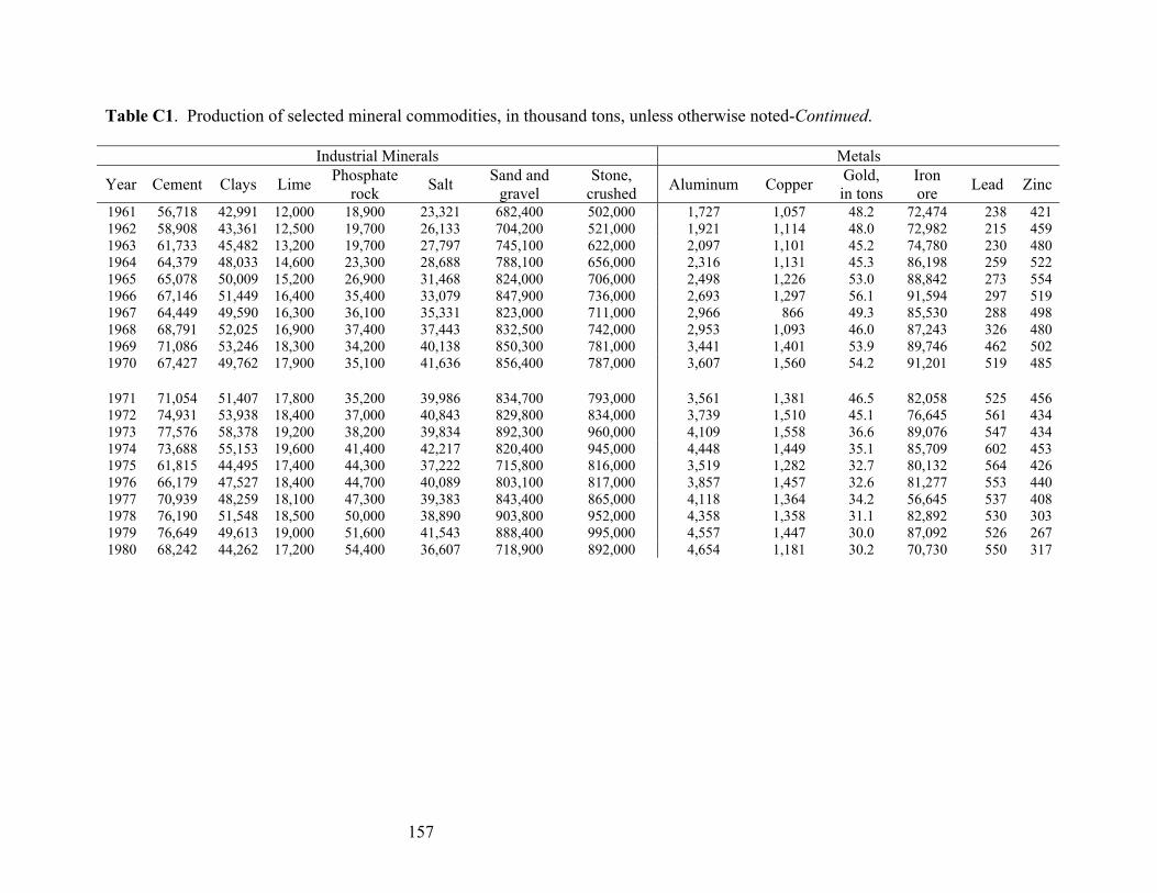
Table C1. Production of selected mineral commodities, in thousand tons, unless otherwise noted-Continued.
Industrial Minerals Metals
Year Cement Clays Lime Phosphate rock Salt Sand and
gravel Stone,
crushed Aluminum Copper Gold, in tons
Iron ore Lead Zinc
1961 56,718 42,991 12,000 18,900 23,321 682,400 502,000 1,727 1,057 48.2 72,474 238 4211962 58,908 43,361 12,500 19,700 26,133 704,200 521,000 1,921 1,114 48.0 72,982 215 4591963 61,733 45,482 13,200 19,700 27,797 745,100 622,000 2,097 1,101 45.2 74,780 230 4801964 64,379 48,033 14,600 23,300 28,688 788,100 656,000 2,316 1,131 45.3 86,198 259 5221965 65,078 50,009 15,200 26,900 31,468 824,000 706,000 2,498 1,226 53.0 88,842 273 5541966 5 67,146 1,449 16,400 35,400 33,079 847,900 736,000 2,693 1,297 56.1 91,594 297 5191967 64,449 49,590 16,300 36,100 35,331 823,000 711,000 2,966 866 49.3 85,530 288 4981968 68,791 52,025 16,900 37,400 37,443 832,500 742,000 2,953 1,093 46.0 87,243 326 4801969 71,086 53,246 18,300 34,200 40,138 850,300 781,000 3,441 1,401 53.9 89,746 462 5021970 67,427 49,762 17,900 35,100 41,636 856,400 787,000 3,607 1,560 54.2 91,201 519 485
1971 71,054 51,407 17,800 35,200 39,986 834,700 793,000 3,561 1,381 46.5 82,058 525 4561972 74,931 53,938 18,400 37,000 40,843 829,800 834,000 3,739 1,510 45.1 76,645 561 4341973 77,576 58,378 19,200 38,200 39,834 892,300 960,000 4,109 1,558 36.6 89,076 547 4341974 73,688 55,153 19,600 41,400 42,217 820,400 945,000 4,448 1,449 35.1 85,709 602 4531975 61,815 44,495 17,400 44,300 37,222 715,800 816,000 3,519 1,282 32.7 80,132 564 4261976 66,179 47,527 18,400 44,700 40,089 803,100 817,000 3,857 1,457 32.6 81,277 553 4401977 70,939 48,259 18,100 47,300 39,383 843,400 865,000 4,118 1,364 34.2 56,645 537 4081978 76,190 51,548 18,500 50,000 38,890 903,800 952,000 4,358 1,358 31.1 82,892 530 3031979 76,649 49,613 19,000 51,600 41,543 888,400 995,000 4,557 1,447 30.0 87,092 526 2671980 68,242 44,262 17,200 54,400 36,607 718,900 892,000 4,654 1,181 30.2 70,730 550 317
157
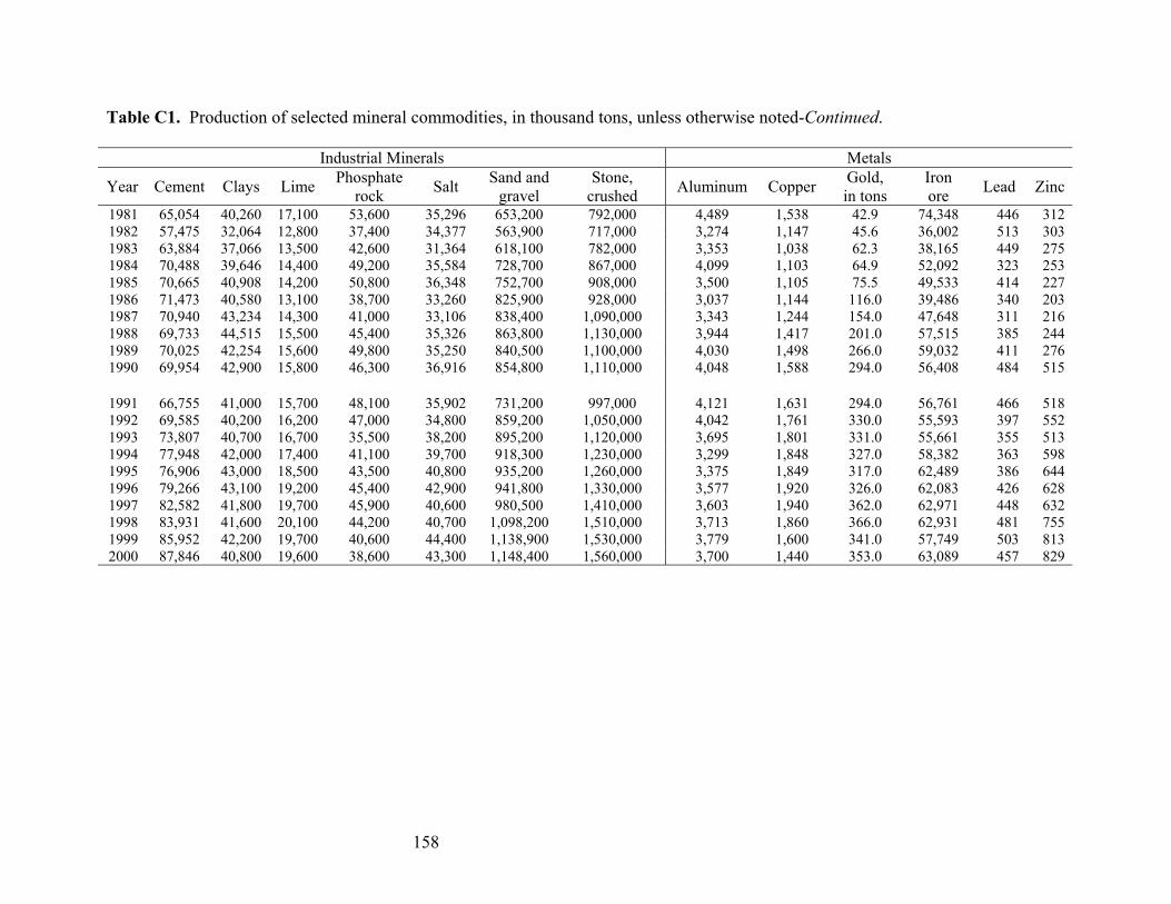
Table C1. Production of selected mineral commodities, in thousand tons, unless otherwise noted-Continued.
Industrial Minerals Metals
Year Cement Clays Lime Phosphate rock Salt Sand and
gravel Stone,
crushed Aluminum Copper Gold, in tons
Iron ore Lead Zinc
1981 65,054 40,260 17,100 53,600 35,296 653,200 792,000 4,489 1,538 42.9 74,348 446 3121982 57,475 32,064 12,800 37,400 34,377 563,900 717,000 3,274 1,147 45.6 36,002 513 3031983 63,884 37,066 13,500 42,600 31,364 618,100 782,000 3,353 1,038 62.3 38,165 449 2751984 70,488 39,646 14,400 49,200 35,584 728,700 867,000 4,099 1,103 64.9 52,092 323 2531985 70,665 40,908 14,200 50,800 36,348 752,700 908,000 3,500 1,105 75.5 49,533 414 2271986 71,473 40,580 13,100 38,700 33,260 825,900 928,000 3,037 1,144 116.0 39,486 340 2031987 70,940 43,234 14,300 41,000 33,106 838,400 1,090,000 3,343 1,244 154.0 47,648 311 2161988 69,733 44,515 15,500 45,400 35,326 863,800 1,130,000 3,944 1,417 201.0 57,515 385 2441989 70,025 42,254 15,600 49,800 35,250 840,500 1,100,000 4,030 1,498 266.0 59,032 411 2761990 69,954 42,900 15,800 36,916 854,800 1,110,000 4,048 1,588 294.0 56,408 484 515
1991 66,755 41,000 15,700 48,100 35,902 731,200 997,000 4,121 1,631 294.0 56,761 466 5181992 69,585 40,200 16,200 47,000 34,800 859,200 1,050,000 4,042 1,761 330.0 55,593 397 5521993 73,807 40,700 16,700 35,500 38,200 895,200 1,120,000 3,695 1,801 331.0 55,661 355 5131994 77,948 42,000 17,400 41,100 39,700 918,300 1,230,000 3,299 1,848 327.0 58,382 363 5981995 76,906 43,000 18,500 43,500 40,800 935,200 1,260,000 3,375 1,849 317.0 62,489 386 6441996 79,266 43,100 19,200 45,400 42,900 941,800 1,330,000 3,577 1,920 326.0 62,083 426 6281997 82,582 41,800 19,700 45,900 40,600 980,500 1,410,000 3,603 1,940 362.0 62,971 448 6321998 83,931 41,600 20,100 44,200 40,700 1,098,200 1,510,000 3,713 1,860 366.0 62,931 481 7551999 85,952 42,200 19,700 40,600 44,400 1,138,900 1,530,000 3,779 1,600 341.0 57,749 503 8132000 87,846 40,800 19,600 38,600 43,300 1,148,400 1,560,000 3,700 1,440 353.0 63,089 457 829
46,300
158
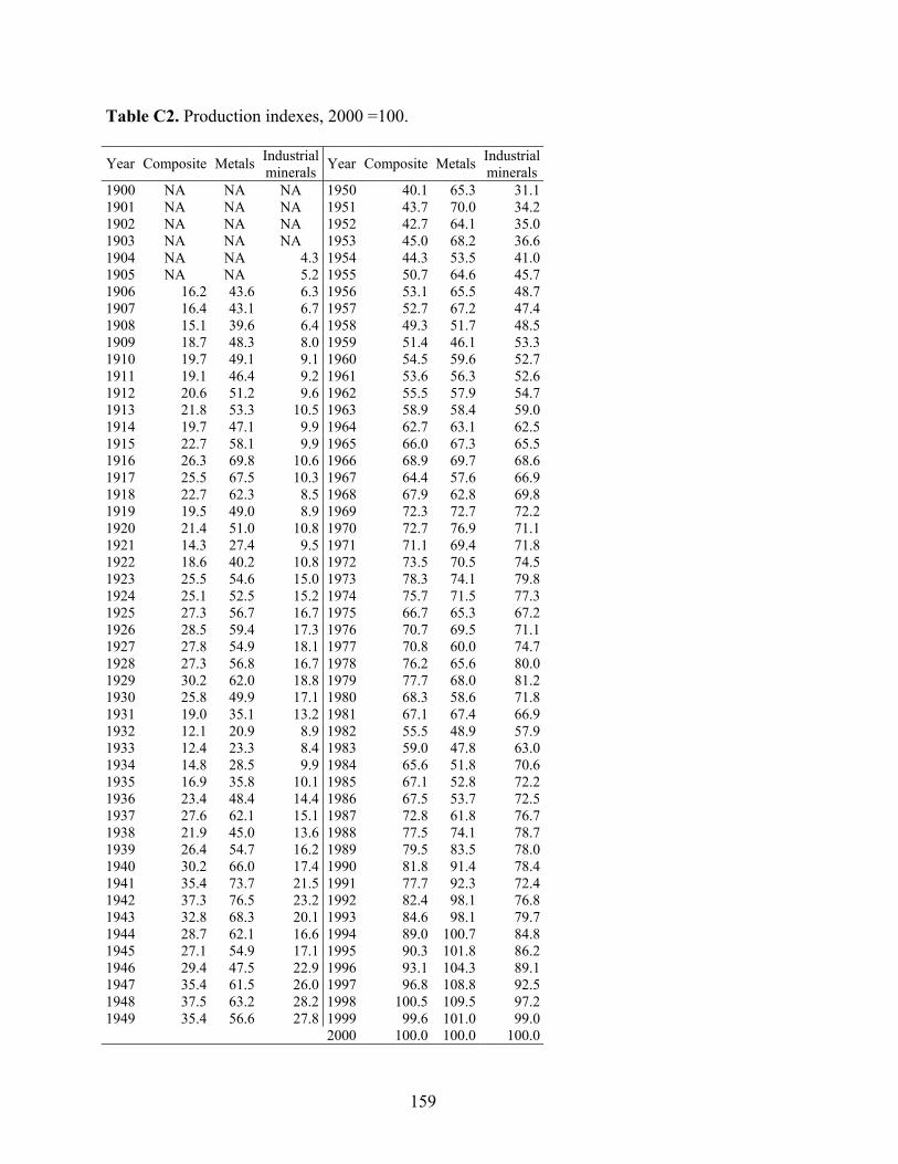
Table C2. Production indexes, 2000 =100.
Industrial IndustrialYear Composite Metals minerals Year Composite Metals minerals1900 NA NA NA 1950 40.1 65.3 31.11901 NA NA NA 1951 43.7 70.0 34.21902 NA NA NA 1952 42.7 64.1 35.01903 NA NA NA 1953 45.0 68.2 36.61904 NA NA 4.3 1954 44.3 53.5 41.01905 NA NA 5.2 1955 50.7 64.6 45.71906 16.2 43.6 6.3 1956 53.1 65.5 48.71907 16.4 43.1 6.7 1957 52.7 67.2 47.41908 15.1 39.6 6.4 1958 49.3 51.7 48.51909 18.7 48.3 8.0 1959 51.4 46.1 53.31910 19.7 49.1 9.1 1960 54.5 59.6 52.71911 19.1 46.4 9.2 1961 53.6 56.3 52.61912 20.6 51.2 9.6 1962 55.5 57.9 54.71913 21.8 53.3 10.5 1963 58.9 58.4 59.01914 19.7 47.1 9.9 1964 62.7 63.1 62.51915 22.7 58.1 9.9 1965 66.0 67.3 65.51916 26.3 69.8 10.6 1966 68.9 69.7 68.61917 25.5 67.5 10.3 1967 64.4 57.6 66.91918 22.7 62.3 8.5 1968 67.9 62.8 69.81919 19.5 49.0 8.9 1969 72.3 72.7 72.21920 21.4 51.0 10.8 1970 72.7 76.9 71.11921 14.3 27.4 9.5 1971 71.1 69.4 71.81922 18.6 40.2 10.8 1972 73.5 70.5 74.51923 25.5 54.6 15.0 1973 78.3 74.1 79.81924 25.1 52.5 15.2 1974 75.7 71.5 77.31925 27.3 56.7 16.7 1975 66.7 65.3 67.21926 28.5 59.4 17.3 1976 70.7 69.5 71.11927 27.8 54.9 18.1 1977 70.8 60.0 74.71928 27.3 56.8 16.7 1978 76.2 65.6 80.01929 30.2 62.0 18.8 1979 77.7 68.0 81.21930 25.8 49.9 17.1 1980 68.3 58.6 71.81931 19.0 35.1 13.2 1981 67.1 67.4 66.91932 12.1 20.9 8.9 1982 55.5 48.9 57.9
12.4 23.3 8.4 1983 59.0 47.8 63.01934 14.8 28.5 9.9 1984 65.6 51.8 70.61935 16.9 35.8 10.1 1985 67.1 52.8 72.21936 23.4 48.4 14.4 1986 67.5 53.7 72.51937 27.6 62.1 15.1 1987 72.8 61.8 76.71938 21.9 45.0 13.6 1988 77.5 74.1 78.71939 26.4 54.7 16.2 1989 79.5 83.5 78.01940 30.2 66.0 17.4 1990 81.8 91.4 78.41941 35.4 73.7 21.5 1991 77.7 92.3 72.41942 37.3 76.5 23.2 1992 82.4 98.1 76.81943 32.8 68.3 20.1 1993 84.6 98.1 79.71944 28.7 62.1 16.6 1994 89.0 100.7 84.81945 27.1 54.9 17.1 1995 90.3 101.8 86.21946 29.4 47.5 22.9 1996 93.1 104.3 89.11947 35.4 61.5 26.0 1997 96.8 108.8 92.51948 37.5 63.2 28.2 1998 100.5 109.5 97.21949 35.4 56.6 27.8 1999 99.6 101.0 99.0
2000 100.0 100.0 100.0
1933
159
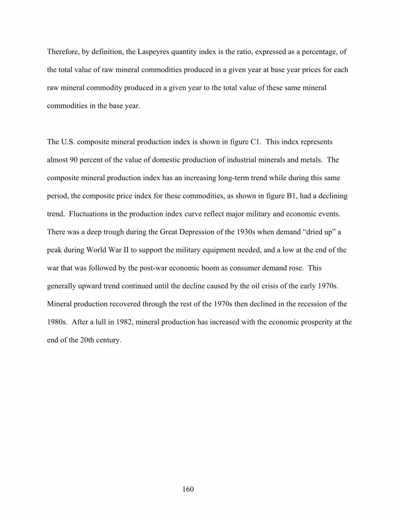
Therefore, by definition, the Laspeyres quantity index is the ratio, expressed as a percentage, of
the total value of raw mineral commodities produced in a given year at base year prices for each
raw mineral commodity produced in a given year to the total value of these same mineral
commodities in the base year.
The U.S. composite mineral production index is shown in figure C1. This index represents
almost 90 percent of the value of domestic production of industrial minerals and metals. The
composite mineral production index has an increasing long-term trend while during this same
period, the composite price index for these commodities, as shown in figure B1, had a declining
trend. Fluctuations in the production index curve reflect major military and economic events.
There was a deep trough during the Great Depression of the 1930s when demand “dried up” a
peak during World War II to support the military equipment needed, and a low at the end of the
war that was followed by the post-war economic boom as consumer demand rose. This
generally upward trend continued until the decline caused by the oil crisis of the early 1970s.
Mineral production recovered through the rest of the 1970s then declined in the recession of the
1980s. After a lull in 1982, mineral production has increased with the economic prosperity at the
end of the 20th century.
160
0
20
40
60
80
100
120
1900 1910 1920 1930 1940 1950 1960 1970 1980 1990 2000
YEAR
U.S.
CO
MPO
SITE
MIN
ERA
L PR
OD
UCTI
ON
IND
EX20
00 =
100
Index Linear trend
Figure C1. U.S. composite mineral production index, 1906-2000.
The industrial mineral production index (figure C2) has a similar profile, and growth trend, as
the composite production index because it comprises two-thirds of the composite index.
Production of the industrial minerals is closely tied to in overall economic activity. The 20th
century was a time of economic expansion. Industrial minerals grew as a basic part of the
economy. A discussion of the trends of the individual commodities comprising the industrial
minerals production index follows. It should be noted that the linear trend line in figure C2 is
not shown prior to 1910 because it is less than zero. The linear trend is the average trend for the
entire series. In this case, the slope of the average trend results in the trend line being below zero
161

prior to 1910. This does not indicate negative production, but demonstrates that the trend line is
not applicable to the early part of the data series.
0
20
40
60
80
100
120
1900 1910 1920 1930 1940 1950 1960 1970 1980 1990 2000
YEAR
U.S.
INDU
STRI
AL M
INER
AL P
RODU
CTIO
N IN
DEX,
200
0 =
100
Index Linear trend
Figure C2. U.S. industrial mineral production index, 1904-2000.
Cement accounts for more than 20 percent of the value of production of industrial minerals
included in the composite index and in 2000 was the industrial mineral with the second largest
value of mine production in the United States ($6,901 million), see table B1. Most cement was
used in the construction of bridges, buildings, highways, and other infrastructure. Cement
production expanded during the 20th century along with the construction industry as part of the
growing economy. Figure C3 shows the strong increase cement production. Production
162
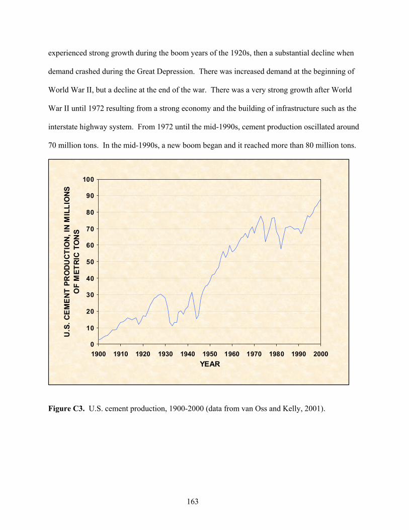
experienced strong growth during the boom years of the 1920s, then a substantial decline when
demand crashed during the Great Depression. There was increased demand at the beginning of
World War II, but a decline at the end of the war. There was a very strong growth after World
War II until 1972 resulting from a strong economy and the building of infrastructure such as the
interstate highway system. From 1972 until the mid-1990s, cement production oscillated around
70 million tons. In the mid-1990s, a new boom began and it reached more than 80 million tons.
0
10
20
30
40
50
60
70
80
90
100
1900 1910 1920 1930 1940 1950 1960 1970 1980 1990 2000YEAR
U.S
. CEM
ENT
PRO
DUCT
ION,
IN M
ILLI
ONS
O
F M
ETRI
C T
ON
S
Figure C3. U.S. cement production, 1900-2000 (data from van Oss and Kelly, 2001).
163
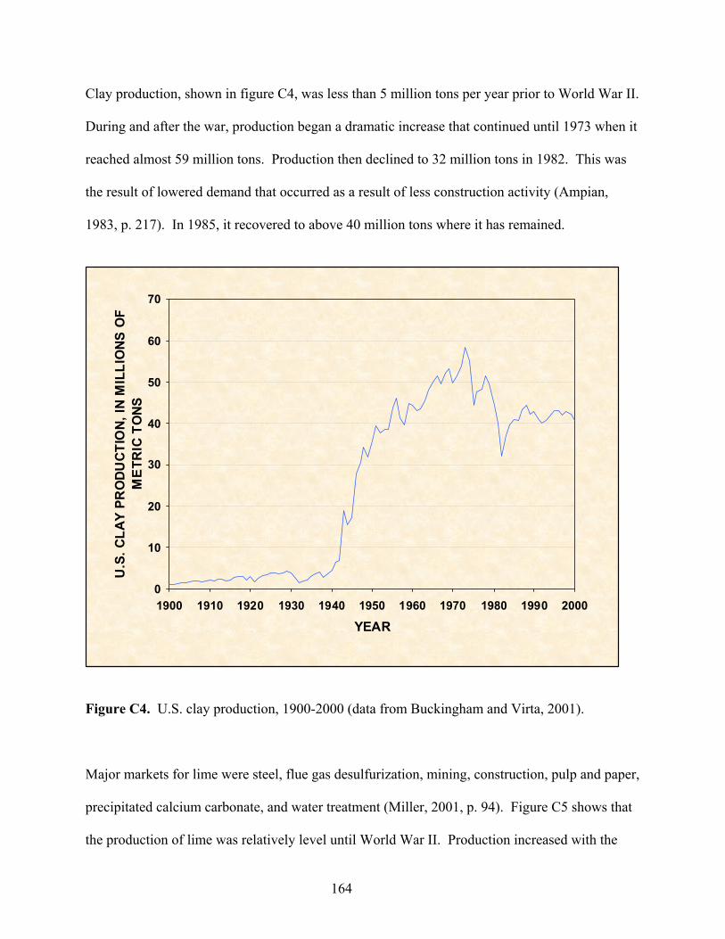
Clay production, shown in figure C4, was less than 5 million tons per year prior to World War II.
During and after the war, production began a dramatic increase that continued until 1973 when it
reached almost 59 million tons. Production then declined to 32 million tons in 1982. This was
the result of lowered demand that occurred as a result of less construction activity (Ampian,
1983, p. 217). In 1985, it recovered to above 40 million tons where it has remained.
0
10
20
30
40
50
60
70
1900 1910 1920 1930 1940 1950 1960 1970 1980 1990 2000
YEAR
U.S
. CLA
Y PR
ODU
CTIO
N, IN
MIL
LIO
NS O
F M
ETR
IC T
ONS
Figure C4. U.S. clay production, 1900-2000 (data from Buckingham and Virta, 2001).
Major markets for lime were steel, flue gas desulfurization, mining, construction, pulp and paper,
precipitated calcium carbonate, and water treatment (Miller, 2001, p. 94). Figure C5 shows that
the production of lime was relatively level until World War II. Production increased with the
164
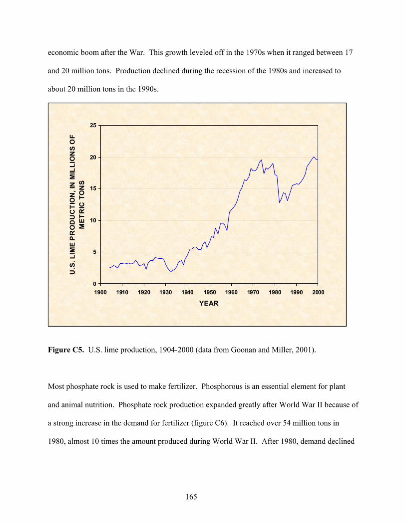
economic boom after the War. This growth leveled off in the 1970s when it ranged between 17
and 20 million tons. Production declined during the recession of the 1980s and increased to
about 20 million tons in the 1990s.
0
5
10
15
20
25
1900 1910 1920 1930 1940 1950 1960 1970 1980 1990 2000
YEAR
U.S
. LIM
E P
RO
DU
CTI
ON
, IN
MIL
LIO
NS
OF
MET
RIC
TO
NS
Figure C5. U.S. lime production, 1904-2000 (data from Goonan and Miller, 2001).
Most phosphate rock is used to make fertilizer. Phosphorous is an essential element for plant
and animal nutrition. Phosphate rock production expanded greatly after World War II because of
a strong increase in the demand for fertilizer (figure C6). It reached over 54 million tons in
1980, almost 10 times the amount produced during World War II. After 1980, demand declined
165
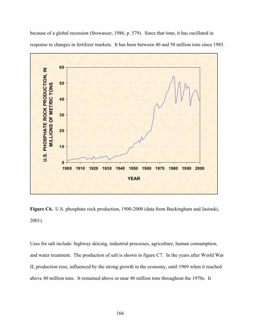
because of a global recession (Stowasser, 1986, p. 579). Since that time, it has oscillated in
response to changes in fertilizer markets. It has been between 40 and 50 million tons since 1985.
0
10
20
30
40
50
60
1900 1910 1920 1930 1940 1950 1960 1970 1980 1990 2000
YEAR
U.S
. PH
OSP
HATE
RO
CK P
RO
DUC
TIO
N, IN
M
ILLI
ON
S O
F M
ETRI
C TO
NS
Figure C6. U.S. phosphate rock production, 1900-2000 (data from Buckingham and Jasinski,
2001).
Uses for salt include: highway deicing, industrial processes, agriculture, human consumption,
and water treatment. The production of salt is shown in figure C7. In the years after World War
II, production rose, influenced by the strong growth in the economy, until 1969 when it reached
above 40 million tons. It remained above or near 40 million tons throughout the 1970s. It
166
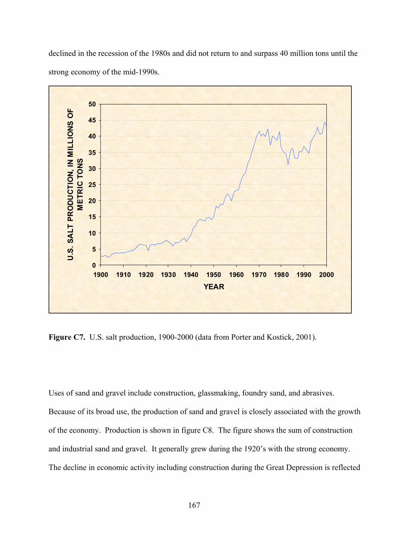
declined in the recession of the 1980s and did not return to and surpass 40 million tons until the
strong economy of the mid-1990s.
0
5
10
15
20
25
30
35
40
45
50
1900 1910 1920 1930 1940 1950 1960 1970 1980 1990 2000
YEAR
U.S
. SA
LT P
RO
DUCT
ION,
IN M
ILLI
ONS
OF
MET
RIC
TO
NS
Figure C7. U.S. salt production, 1900-2000 (data from Porter and Kostick, 2001).
Uses of sand and gravel include construction, glassmaking, foundry sand, and abrasives.
Because of its broad use, the production of sand and gravel is closely associated with the growth
of the economy. Production is shown in figure C8. The figure shows the sum of construction
and industrial sand and gravel. It generally grew during the 1920’s with the strong economy.
The decline in economic activity including construction during the Great Depression is reflected
167
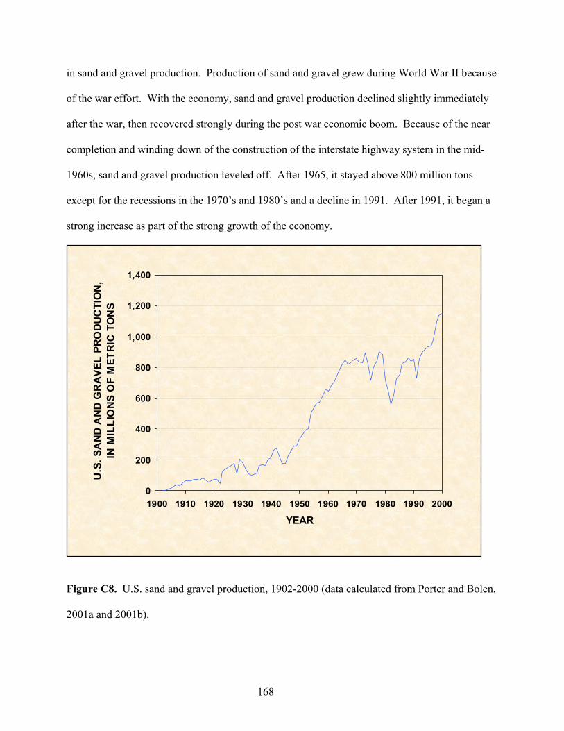
in sand and gravel production. Production of sand and gravel grew during World War II because
of the war effort. With the economy, sand and gravel production declined slightly immediately
after the war, then recovered strongly during the post war economic boom. Because of the near
completion and winding down of the construction of the interstate highway system in the mid-
1960s, sand and gravel production leveled off. After 1965, it stayed above 800 million tons
except for the recessions in the 1970’s and 1980’s and a decline in 1991. After 1991, it began a
strong increase as part of the strong growth of the economy.
0
200
400
600
800
1,000
1,200
1,400
1900 1910 1920 1930 1940 1950 1960 1970 1980 1990 2000
YEAR
U.S
. SA
ND A
ND G
RAV
EL P
RODU
CTI
ON
, IN
MIL
LIO
NS O
F M
ETRI
C T
ON
S
Figure C8. U.S. sand and gravel production, 1902-2000 (data calculated from Porter and Bolen,
2001a and 2001b).
168
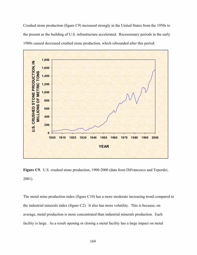
Crushed stone production (figure C9) increased strongly in the United States from the 1950s to
the present as the building of U.S. infrastructure accelerated. Recessionary periods in the early
1980s caused decreased crushed stone production, which rebounded after this period.
0
200
400
600
800
1,000
1,200
1,400
1,600
1,800
1900 1910 1920 1930 1940 1950 1960 1970 1980 1990 2000
YEAR
U.S.
CRU
SHED
STO
NE P
RODU
CTI
ON,
IN
MIL
LIO
NS O
F M
ETRI
C T
ONS
Figure C9. U.S. crushed stone production, 1900-2000 (data from DiFrancesco and Tepordei,
2001).
The metal mine production index (figure C10) has a more moderate increasing trend compared to
the industrial minerals index (figure C2). It also has more volatility. This is because, on
average, metal production is more concentrated than industrial minerals production. Each
facility is large. As a result opening or closing a metal facility has a large impact on metal
169

production. Generally industrial minerals industries are made up of a large number of smaller
operations. The opening or closing of a smaller operation does not cause dramatic changes in
industrial minerals production. This results in more volatile adjustments in metal production.
The metal production index has a large dip during the years of the Great Depression following
the sudden drop in demand for goods and services. It then has a relatively level trend from
World War II through 1979. After a valley in the 1980s recession, it has risen substantially
through 1998 because of strong advances in the economy. The trends of individual metal
commodities are discussed below.
0
20
40
60
80
100
120
1900 1910 1920 1930 1940 1950 1960 1970 1980 1990 2000
YEAR
U.S
. MET
AL
MIN
E PR
ODU
CTIO
N IN
DEX,
20
00 =
100
Index Linear trend
Figure C10. U.S. metal mine production index, 1906-2000.
170
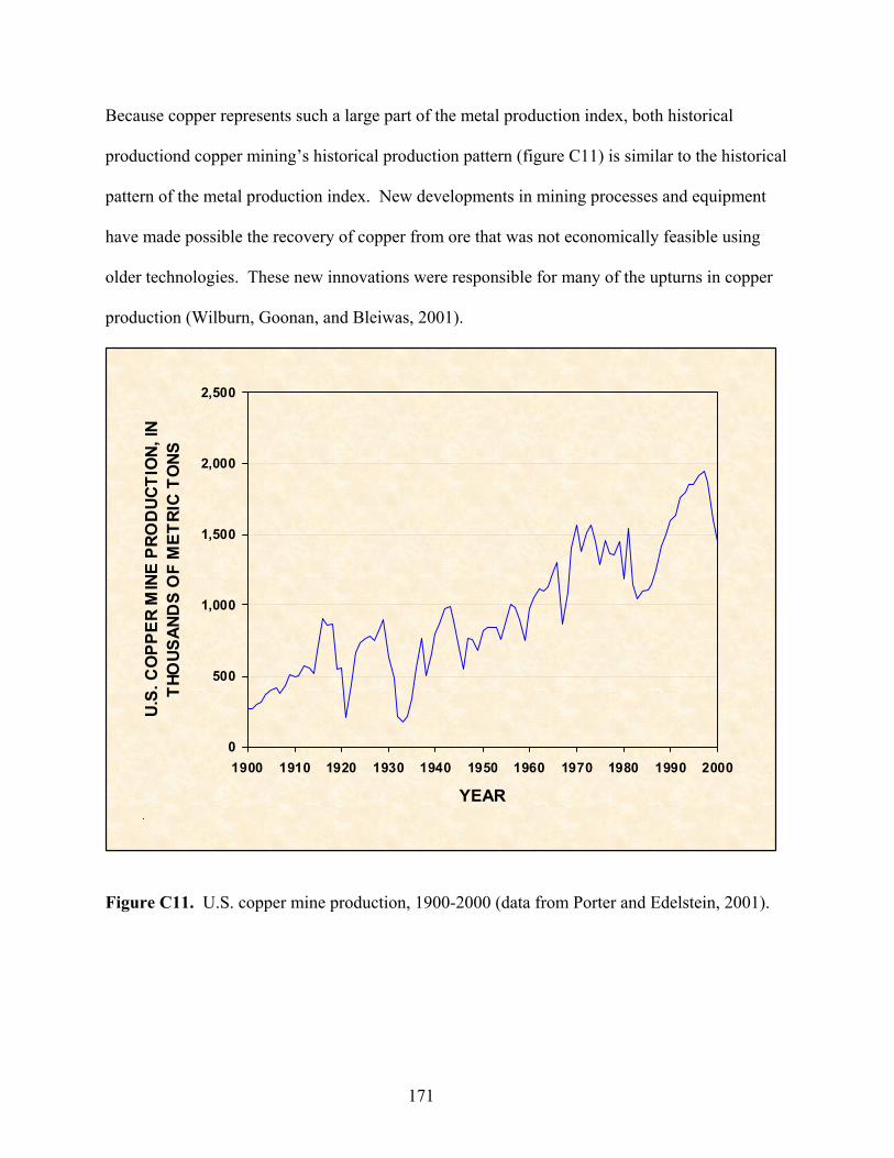
Because copper represents such a large part of the metal production index, both historical
productiond copper mining’s historical production pattern (figure C11) is similar to the historical
pattern of the metal production index. New developments in mining processes and equipment
have made possible the recovery of copper from ore that was not economically feasible using
older technologies. These new innovations were responsible for many of the upturns in copper
production (Wilburn, Goonan, and Bleiwas, 2001).
0
500
1,000
1,500
2,000
2,500
1900 1910 1920 1930 1940 1950 1960 1970 1980 1990 2000
YEAR
U.S.
CO
PPER
MIN
E PR
OD
UCTI
ON,
IN
THO
USAN
DS
OF
MET
RIC
TONS
.
Figure C11. U.S. copper mine production, 1900-2000 (data from Porter and Edelstein, 2001).
171

Mine production for most of the metals included in the index have increasing long-term trends.
Gold mine production (figure C12) has been level to declining, except for a peak that occurred
when the government increased the price of gold in 1934. The period of relatively high prices
ended in 1942 because U.S. gold mines were ordered closed during World War II so that
equipment supplies and labor could be focused on essential base metals. Production remained at
this low level after the war because of increased costs associated with reopening closed mines
(Lucas, 1986, p. 323). In the early 1980s, gold production began a sharp rise as inflation
worries stirred speculation. In addition, new technologies, such as the heap leach method, played
a significant role in this dramatic increase. Disseminated deposits were identified as a source of
gold in the 1960s. Most of them have been found in California, Nevada, and Utah, where gold is
often recovered by heap leaching (Boyle, 1994). The increase in production continued through
the 1990s due to high global demand for more gold.
172
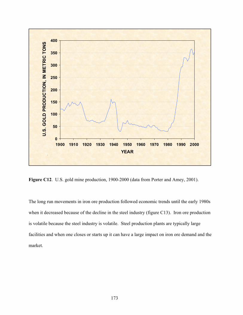
0
50
100
150
200
250
300
350
400
1900 1910 1920 1930 1940 1950 1960 1970 1980 1990 2000
YEAR
U.S.
GO
LD P
RODU
CTI
ON
, IN
MET
RIC
TONS
.
Figure C12. U.S. gold mine production, 1900-2000 (data from Porter and Amey, 2001).
The long run movements in iron ore production followed economic trends until the early 1980s
when it decreased because of the decline in the steel industry (figure C13). Iron ore production
is volatile because the steel industry is volatile. Steel production plants are typically large
facilities and when one closes or starts up it can have a large impact on iron ore demand and the
market.
173

0
20
40
60
80
100
120
140
1900 1910 1920 1930 1940 1950 1960 1970 1980 1990 2000
YEAR
U.S.
IRO
N O
RE
PRO
DUC
TIO
N, IN
MIL
LIO
NS
OF
MET
RIC
TO
NS
Figure C13. U.S. iron ore production, 1900-2000 (data from Kelly and Kirk, 2001).
Lead production (figure C14) declined during the Great Depression of the 1930s. It recovered
during World War II, but turned down after the War due to the depletion of reserves in the “lead
belt” in Missouri and Arkansas (Smith, 1999, p. 74). Production increased in 1969 after the first
significant production came into the market from the southeast Missouri lead belt in 1969
(Woodbury, 1985, p. 441). Production was effected by a general slowdown in the economy
during the 1980s. Since that time, lead production has oscillated around 400 thousand tons per
year.
174
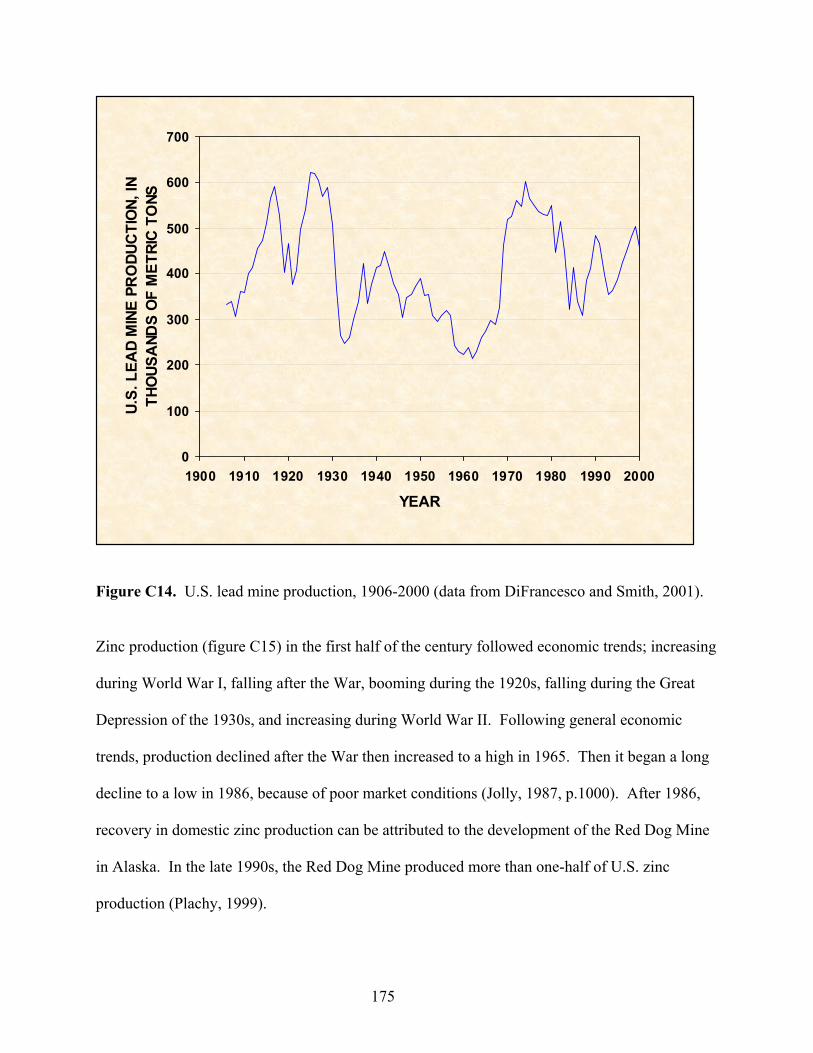
0
100
200
300
400
500
600
700
1900 1910 1920 1930 1940 1950 1960 1970 1980 1990 2000
YEAR
U.S.
LEA
D M
INE
PRO
DUC
TIO
N, IN
TH
OUS
AND
S O
F M
ETRI
C T
ONS
Figure C14. U.S. lead mine production, 1906-2000 (data from DiFrancesco and Smith, 2001).
Zinc production (figure C15) in the first half of the century followed economic trends; increasing
during World War I, falling after the War, booming during the 1920s, falling during the Great
Depression of the 1930s, and increasing during World War II. Following general economic
trends, production declined after the War then increased to a high in 1965. Then it began a long
decline to a low in 1986, because of poor market conditions (Jolly, 1987, p.1000). After 1986,
recovery in domestic zinc production can be attributed to the development of the Red Dog Mine
in Alaska. In the late 1990s, the Red Dog Mine produced more than one-half of U.S. zinc
production (Plachy, 1999).
175
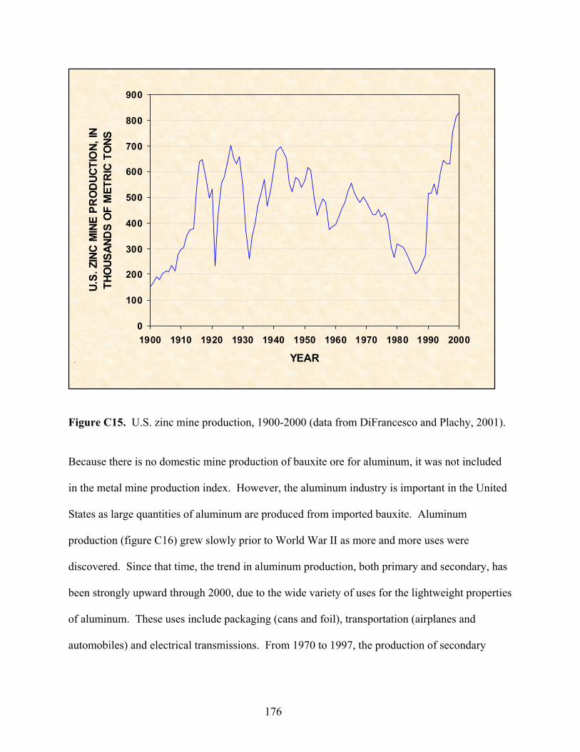
0
100
200
300
400
500
600
700
800
900
1900 1910 1920 1930 1940 1950 1960 1970 1980 1990 2000
YEAR
U.S.
ZIN
C M
INE
PRO
DUC
TIO
N, IN
TH
OUS
AND
S O
F M
ETR
IC T
ONS
.
Figure C15. U.S. zinc mine production, 1900-2000 (data from DiFrancesco and Plachy, 2001).
Because there is no domestic mine production of bauxite ore for aluminum, it was not included
in the metal mine production index. However, the aluminum industry is important in the United
States as large quantities of aluminum are produced from imported bauxite. Aluminum
production (figure C16) grew slowly prior to World War II as more and more uses were
discovered. Since that time, the trend in aluminum production, both primary and secondary, has
been strongly upward through 2000, due to the wide variety of uses for the lightweight properties
of aluminum. These uses include packaging (cans and foil), transportation (airplanes and
automobiles) and electrical transmissions. From 1970 to 1997, the production of secondary
176
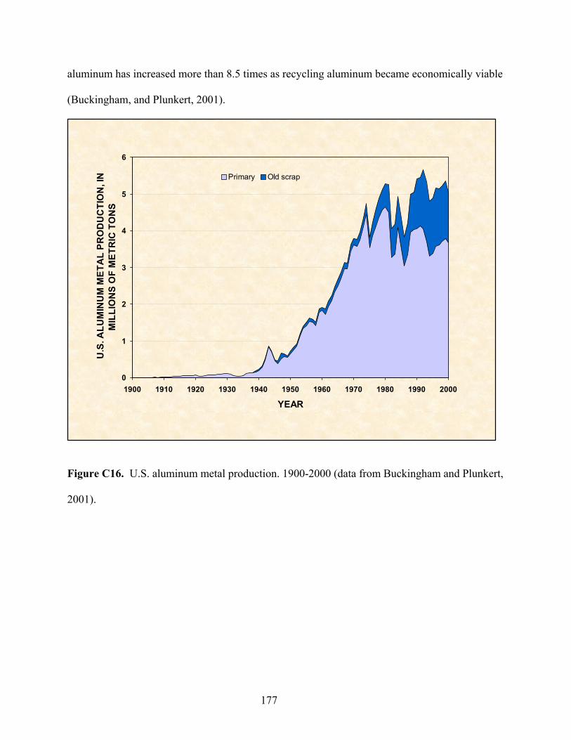
aluminum has increased more than 8.5 times as recycling aluminum became economically viable
(Buckingham, and Plunkert, 2001).
0
1
2
3
4
5
6
1900 1910 1920 1930 1940 1950 1960 1970 1980 1990 2000
YEAR
U.S
. ALU
MIN
UM
MET
AL
PRO
DU
CTI
ON
, IN
MIL
LIO
NS
OF
MET
RIC
TO
NS
Primary Old scrap
Figure C16. U.S. aluminum metal production. 1900-2000 (data from Buckingham and Plunkert,
2001).
177
References
Ampian, S.G., 1983, Clays, in Metals and Minerals: U.S. Bureau of Mines Minerals Yearbook 1982, v. I, p. 217-248. Boyle, E.H., 1994, World gold– A minerals availability appraisal: U.S. Bureau of Mines Special Publication SP24-94, 197 p. Buckingham, D.A., and Jasinski, S.M., 2001, Phosphate rock statistics, in Historical statistics for mineral commodities in the United States: U.S. Geological Survey Open-File Report 01-006. Buckingham, D.A., and Plunkert, P.A., 2001, Aluminum statistics in Historical statistics for mineral commodities in the United States: U.S. Geological Survey Open-File Report 01-006. Buckingham, D.A., and Virta, R.L., 2001, Clay statistics, in Historical statistics for mineral commodities in the United States: U.S. Geological Survey Open-File Report 01-006. DiFrancesco, C.A., and Plachy, Jozef, 2001, Zinc statistics, in Historical statistics for mineral commodities in the United States: U.S. Geological Survey Open-File Report 01-006. DiFrancesco, C.A., and Smith, G.R., 2001, Lead statistics, in Historical statistics for mineral commodities in the United States: U.S. Geological Survey Open-File Report 01-006. DiFrancesco, C.A., and Tepordei, V.V., 2001, Stone (crushed) statistics, in Historical statistics for mineral commodities in the United States: U.S. Geological Survey Open-File Report 01-006. Goonan, T.G., and Miller, M.M., 2001, Lime statistics, in Historical statistics for mineral commodities in the United States: U.S. Geological Survey Open-File Report 01-006. Jolly, J. H., 1987, Zinc, in Metals and Minerals: U.S. Bureau of Mines Minerals Yearbook 1986, v. I, p. 999-1025. Lucas, J.M., 1986, Gold, in Mineral Facts and Problems, 1985 edition: U.S. Bureau of Mines Bulletin 675, p. 323-338. Kelly, T.D., and Kirk, D.L., 2001, Iron ore statistics, in Historical statistics for mineral commodities in the United States: U.S. Geological Survey Open-File Report 01-006. Mansfield, Edwin, 1987, Statistics for business and economics, methods and applications, 3rd edition: New York, W.W. Norton & Company, 698 p. Miller, M.M., 2001, Lime, in Mineral Commodity Summaries, 2001: U.S. Geological Survey, p. 94-95.
178

Plachy, Jozef, 1999, Zinc, in Metals and Minerals: U.S. Geological Survey Minerals Yearbook 1998, v. I. p. 85.1-85.18. Porter, K.E., and Amey, E.B., 2001, Gold statistics, in Historical statistics for mineral commodities in the United States: U.S. Geological Survey Open-File Report 01-006. Porter, K.E., and Bolen, W.P., 2001a, Sand and gravel (construction) statistics, in Historical statistics for mineral commodities in the United States: U.S. Geological Survey Open-File Report 01-006. Porter, K.E., and Bolen, W.P., 2001b, Sand and gravel (industrial) statistics, in Historical statistics for mineral commodities in the United States: U.S. Geological Survey Open-File Report 01-006. Porter, K.E., and Edelstein, D.L., 2001, Copper statistics, in Historical statistics for mineral commodities in the United States: U.S. Geological Survey Open-File Report 01-006. Porter, K.E., and Kostick, D.S., 2001, Salt statistics, in Historical statistics for mineral commodities in the United States: U.S. Geological Survey Open-File Report 01-006. Smith G.R., 1999, Lead, in Metal prices in the United States through 1998: U.S. Geological Survey, p. 73-74. Stowasser, W.F. 1986, Phosphate rock, in Mineral Facts and Problems, 1985 edition: U.S. Bureau of Mines Bulletin 675, p. 579. U.S. Geological Survey, 2001, Historical statistics for mineral commodities in the United States: U.S. Geological Survey Open-File Report 01-006. Van Oss, H.G., and Kelly, T.D., 2001, Cement statistics, in Historical statistics for mineral commodities in the United States: U.S. Geological Survey Open-File Report 01-006. Wilburn, D.A., Goonan, T.G., and Bleiwas, D.A., 2001, Technological advancement -- A factor in increasing resource use: U.S. Geological Survey Open-File Report 01-197. Woodbury, W.D. 1985, Lead, in Mineral Facts and Problems, 1985 edition: U.S. Bureau of Mines Bulletin 675, p. 441.
179
APPENDIX D: ECONOMIC CASE STUDY – ALUMINUM
Introduction/background
At least one aluminum compound has been in use for centuries. Alum, KAl(SO4)2 .12H2O, was
used by the Greeks and Romans as an astringent and as a chemical that fixed dyes in cloth
(Banks, 1992). Although aluminum (metal) was isolated in 1827 by Wöhler, it was not until
1886 that an electrolytic process to produce aluminum was discovered independently by Hall in
the United States and by Héroult in France. A chemical process to commercially produce
alumina (aluminum oxide) from bauxite (Bayer Process) was patented by Karl Bayer (Germany)
in 1888.
Aluminum is found in such minerals as alunite, bauxite, kaolinite, and vermiculite. The
aluminum compound, bauxite, is the most important commercial source of aluminum metal. It is
chemically treated to obtain alumina (Al2O3), which is then electrolyzed in a molten salt solution
to yield aluminum. Aluminum is commonly alloyed with various other materials including
copper, magnesium, or zinc, to provide a wide range of physical properties. The heavy reliance
of the transportation industry on aluminum alloys is a testimonial to the efficiency of this
material. The combination of high strength, low weight, high corrosion resistance, and
workability are features that make aluminum alloys a top choice as structural materials. Some of
the more common uses of aluminum are for beverage cans, as packaging materials, and in
automobiles. Recyclability, cost, and low weight for improved fuel economies drive automotive
180
demands. Other less common uses for aluminum (alloys) are: bridges, highway signs, kitchen
utensils, nails, and many other items.
The modern aluminum industry is composed of two principal producing segments, the primary
industry and the recycling industry. Their interrelationships are shown in figure D1. The
primary aluminum industry consists of mining to produce bauxite, refining to produce alumina,
and smelting to produce aluminum metal. The aluminum recycling industry consists of the scrap
industry and secondary smelters and fabricators. Within the recycling industry, are the beverage
can recyclers, which is a distinct industry, and those who recycle other products.
181
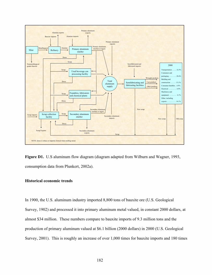
Mine Refinery
Scrap collection facility
Foundries, fabricators and chemical plants
Used beverage can processing facility
Secondary aluminum smelter
Total aluminum
supply
Primary aluminum smelter
Semifabricating and fabricating facilities
Nonmetallurgical grades bauxite
Metallurgical Alumina
Alumina exports
Bauxite imports Alumina imports
Primary aluminum exports
Scrap imports Scrap
Scrap
Scrap
Scrap
Dross
Dross
Secondary aluminum exports
Secondary aluminum imports
New scrap
New scrap Old scrap
Scrap
Primary aluminum imports
Semifabricated and fabricated imports
Wrought products
Cast products
Other products
Scrap Exports
Dross
Dross
Secondary aluminum (molten or ingot)
Primary aluminum (molten or ingot)
Consuming industries
Containers and
packaging …..…….. 20.4%
Building and
construction ……… 13.1%
Transportation ……. 32.5%
Electrical ………….. 6.9%
Consumer durables .. 6.9%
Machinery and
equipment ………… 6.1%
Other, including
exports ..….....……. 14.1%
2000
NOTE: dross is refuse or impurity formed when melting metal.
Figure D1. U.S aluminum flow diagram (diagram adapted from Wilburn and Wagner, 1993,
consumption data from Plunkert, 2002a).
Historical economic trends
In 1900, the U.S. aluminum industry imported 8,800 tons of bauxite ore (U.S. Geological
Survey, 1902) and processed it into primary aluminum metal valued, in constant 2000 dollars, at
almost $34 million. These numbers compare to bauxite imports of 9.3 million tons and the
production of primary aluminum valued at $6.1 billion (2000 dollars) in 2000 (U.S. Geological
Survey, 2001). This is roughly an increase of over 1,000 times for bauxite imports and 180 times
182
the production value of primary aluminum during the twentieth century. Apparent consumption
of aluminum in 1900, equal to the primary aluminum production, was recorded as being slightly
less than 2,300 tons. Almost 8.0 million tons of aluminum (primary metal production plus
recovery from old aluminum scrap plus imports minus exports) were used in 2000 (Plunkert,
2002a), an average annual growth rate of 8.5 percent since 1900.
Prices
Even with these tremendous increases in the use of aluminum, the long-term trend in aluminum
prices (constant 2000$/ ton) has surprisingly decreased. During this time period, there were two
exceptions that exhibited major upward movements (see figure D2). One price peak in 1907
may be partially explained by the increasing demand for both railroad cars and automobiles due
to aluminum’s lightweight and high strength properties. A second factor was the increase in both
copper and tin prices that encouraged manufacturers to substitute aluminum for these metals
where possible, which further increased demand for aluminum. The most pronounced peak in
aluminum prices occurred in 1916 when demand for war materials increased dramatically as the
United States became more involved in World War I. Since that time, the advent of various new
technologies have helped to increase productivity and reduce production costs, which have been
major contributors to the decline of aluminum prices.
183
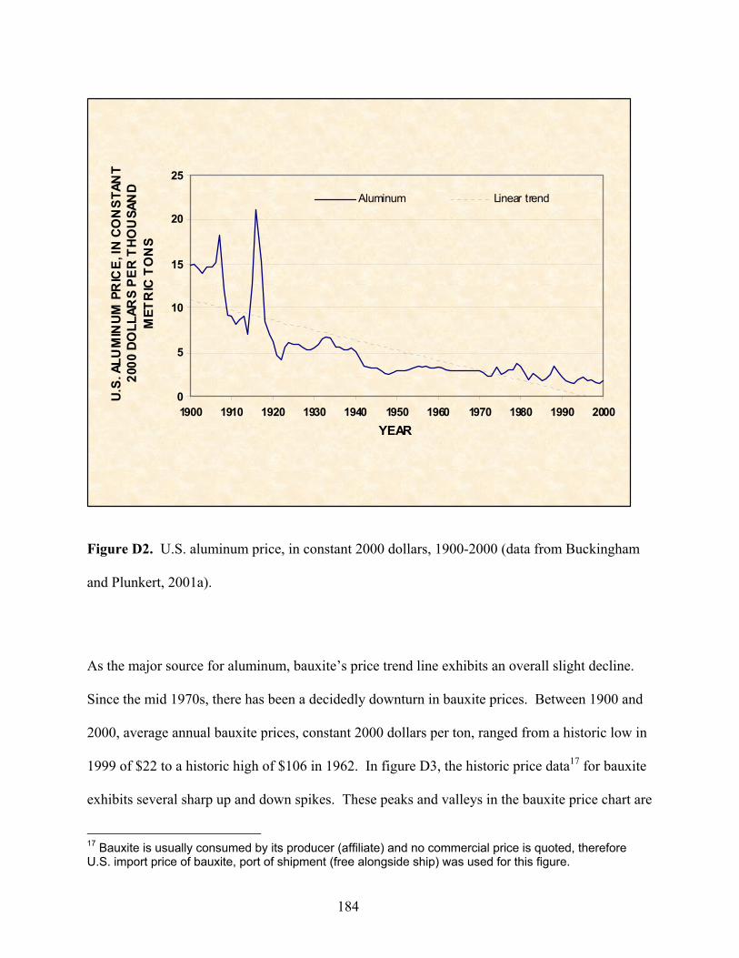
0
5
10
15
20
25
1900 1910 1920 1930 1940 1950 1960 1970 1980 1990 2000YEAR
U.S.
ALU
MIN
UM P
RIC
E, IN
CO
NST
ANT
2000
DO
LLAR
S PE
R TH
OU
SAN
D M
ETR
IC T
ON
S
Aluminum Linear trend
Figure D2. U.S. aluminum price, in constant 2000 dollars, 1900-2000 (data from Buckingham
and Plunkert, 2001a).
As the major source for aluminum, bauxite’s price trend line exhibits an overall slight decline.
Since the mid 1970s, there has been a decidedly downturn in bauxite prices. Between 1900 and
2000, average annual bauxite prices, constant 2000 dollars per ton, ranged from a historic low in
1999 of $22 to a historic high of $106 in 1962. In figure D3, the historic price data17 for bauxite
exhibits several sharp up and down spikes. These peaks and valleys in the bauxite price chart are
17 Bauxite is usually consumed by its producer (affiliate) and no commercial price is quoted, therefore U.S. import price of bauxite, port of shipment (free alongside ship) was used for this figure.
184
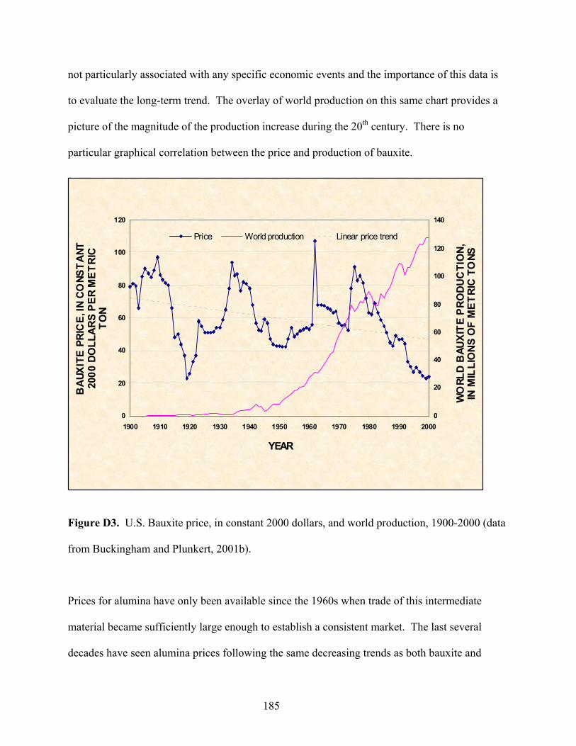
not particularly associated with any specific economic events and the importance of this data is
to evaluate the long-term trend. The overlay of world production on this same chart provides a
picture of the magnitude of the production increase during the 20th century. There is no
particular graphical correlation between the price and production of bauxite.
0
20
40
60
80
100
120
1900 1910 1920 1930 1940 1950 1960 1970 1980 1990 2000
YEAR
BAU
XITE
PRI
CE,
IN C
ONS
TANT
20
00 D
OLL
ARS
PER
MET
RIC
TO
N
0
20
40
60
80
100
120
140
WO
RLD
BAU
XITE
PRO
DUC
TIO
N,
IN M
ILLI
ONS
OF
MET
RIC
TONS
Price World production Linear price trend
Figure D3. U.S. Bauxite price, in constant 2000 dollars, and world production, 1900-2000 (data
from Buckingham and Plunkert, 2001b).
Prices for alumina have only been available since the 1960s when trade of this intermediate
material became sufficiently large enough to establish a consistent market. The last several
decades have seen alumina prices following the same decreasing trends as both bauxite and
185
aluminum. As a value-added product derived from bauxite, but still requiring processing to
become primary aluminum, alumina prices have fallen between the two. One justification for
stable and/or falling alumina prices is because more bauxite producers are incorporating their
own conversion processes to produce and sell alumina. This is usually accomplished within their
organization and at a nearby site rather than shipping the bauxite ore to another location to be
processed by the purchasing firm.
Domestic production
Figure D4 shows the U.S. production of bauxite, alumina, and primary aluminum. Typically,
for every 4.5 tons of bauxite fed into an alumina refinery, approximately 2 tons of alumina are
extracted, from which about 1 ton of primary aluminum is produced (Wilburn and Wagner,
1993). The United States has been mostly dependent on foreign suppliers for metallurgical grade
bauxite. Domestic production of bauxite, which is not normally used for metal production, has
essentially been flat for the last century with one dramatic exception. This enormous increase in
domestic bauxite production occurred during the early 1940s to meet the wartime demand for
aluminum, which was especially critical to the military aircraft industry. Also, a continuous
supply of bauxite from foreign sources was in jeopardy due to a short supply of transport ships
and the possibility of enemy submarine attacks (U.S. Bureau of Mines, 1943). The total
domestic production of bauxite in the 3 war years of 1942, 1943, and 1944 was greater than the
prior 40-year period, from 1900 through 1941. The production peak was in 1943 when over 6.0
million tons were produced. In 1988, the last year that domestic production data on bauxite was
186
available, 588 thousand tons were produced. This was utilized for refractory and other
specialized applications.
Domestic production of alumina reached highs of slightly more than 6.8 million tons in both
1974 and 1980. Since then, alumina production has trended down with approximately 4.8
million tons produced in 2000 (Plunkert, 2002b), a decrease of 16 percent from 1980 levels.
Production trends of alumina and primary aluminum in the United States have moved almost
parallel since the 1950s18.
The major growth period for primary aluminum production in the United States was
concentrated between the beginning of World War II and the 1970s. Military demands initiated
the growth and a recession associated with the oil crisis in the 1970s halted the growth that saw
production of primary aluminum go from slightly less than 200 thousand tons in 1940 to almost
4.5 million tons in 1974, an increase of over 2,000 percent. Since that time, primary aluminum
production has been around the 4.0 million tons level with the indication of a slightly decreasing
trend.
18 Alumina production data was not recorded in the Minerals Yearbook prior to 1950s.
187
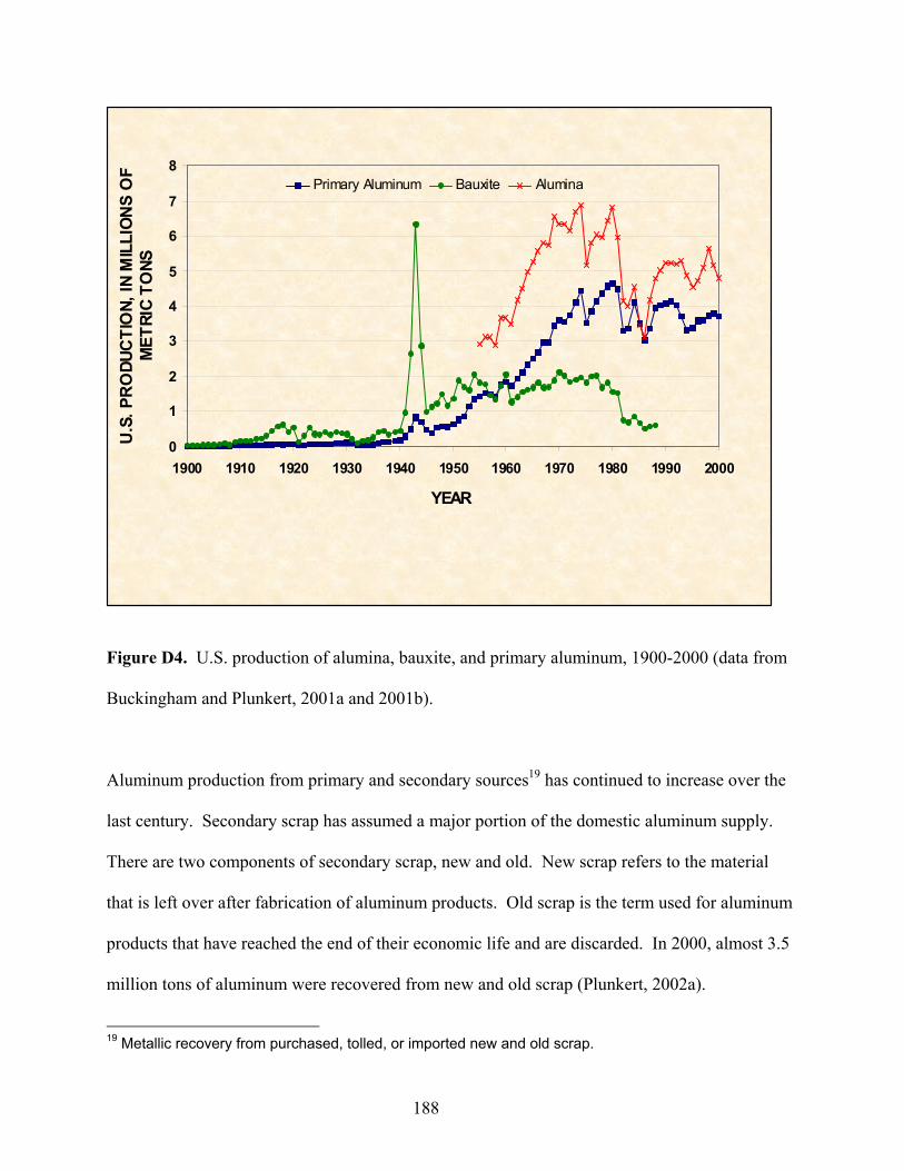
0
1
2
3
4
5
6
7
8
1900 1910 1920 1930 1940 1950 1960 1970 1980 1990 2000
YEAR
U.S
. PR
ODU
CTI
ON,
IN M
ILLI
ON
S O
F M
ETRI
C TO
NS
Primary Aluminum Bauxite Alumina
Figure D4. U.S. production of alumina, bauxite, and primary aluminum, 1900-2000 (data from
Buckingham and Plunkert, 2001a and 2001b).
Aluminum production from primary and secondary sources19 has continued to increase over the
last century. Secondary scrap has assumed a major portion of the domestic aluminum supply.
There are two components of secondary scrap, new and old. New scrap refers to the material
that is left over after fabrication of aluminum products. Old scrap is the term used for aluminum
products that have reached the end of their economic life and are discarded. In 2000, almost 3.5
million tons of aluminum were recovered from new and old scrap (Plunkert, 2002a).
188
19 Metallic recovery from purchased, tolled, or imported new and old scrap.
Viewing the trends of secondary old scrap and primary aluminum production in figure D5,
secondary production has been increasing while primary aluminum production has leveled off.
A widening gap has occurred over the last several decades. Secondary old scrap aluminum
production has become a larger and larger portion of this overall supply and in 2000, represented
over 30 percent of total aluminum production in the United States. Based on worldwide statistics
from the International Aluminium Institute, aluminum recovered from scrap20 has averaged
approximately 10 percent of total aluminum production (aluminum recovered from scrap plus
primary production) from 1996 through 2000 (International Aluminium Institute, 2001§).
20 Aluminum recovered from scrap is the weight of aluminum recovered from purchased or tolled scrap and excludes in-plant (run-around) scrap.
189
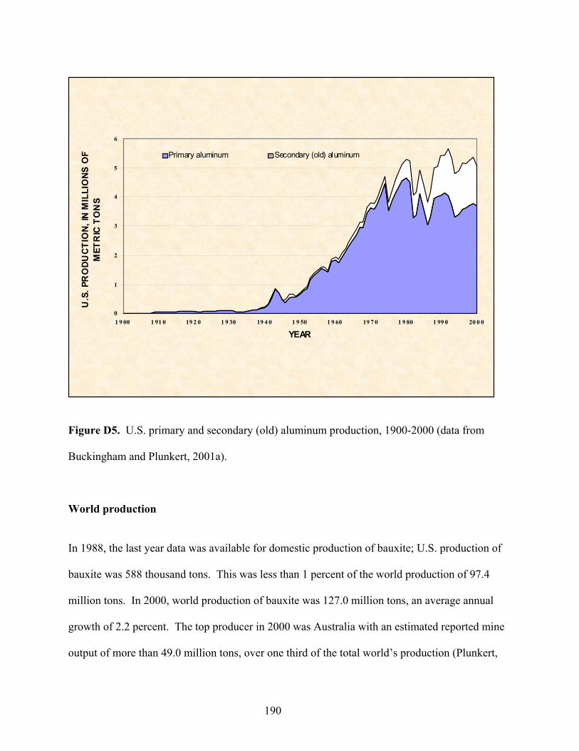
0
1
2
3
4
5
6
1 9 00 1 91 0 19 2 0 1 9 30 19 4 0 1 9 50 1 9 60 19 7 0 1 9 80 1 99 0 20 0 0
YEAR
U.S
. PR
ODU
CTIO
N, IN
MIL
LIO
NS O
F M
ETR
IC T
ON
S
Primary aluminum Secondary (old) aluminum
Figure D5. U.S. primary and secondary (old) aluminum production, 1900-2000 (data from
Buckingham and Plunkert, 2001a).
World production
In 1988, the last year data was available for domestic production of bauxite; U.S. production of
bauxite was 588 thousand tons. This was less than 1 percent of the world production of 97.4
million tons. In 2000, world production of bauxite was 127.0 million tons, an average annual
growth of 2.2 percent. The top producer in 2000 was Australia with an estimated reported mine
output of more than 49.0 million tons, over one third of the total world’s production (Plunkert,
190
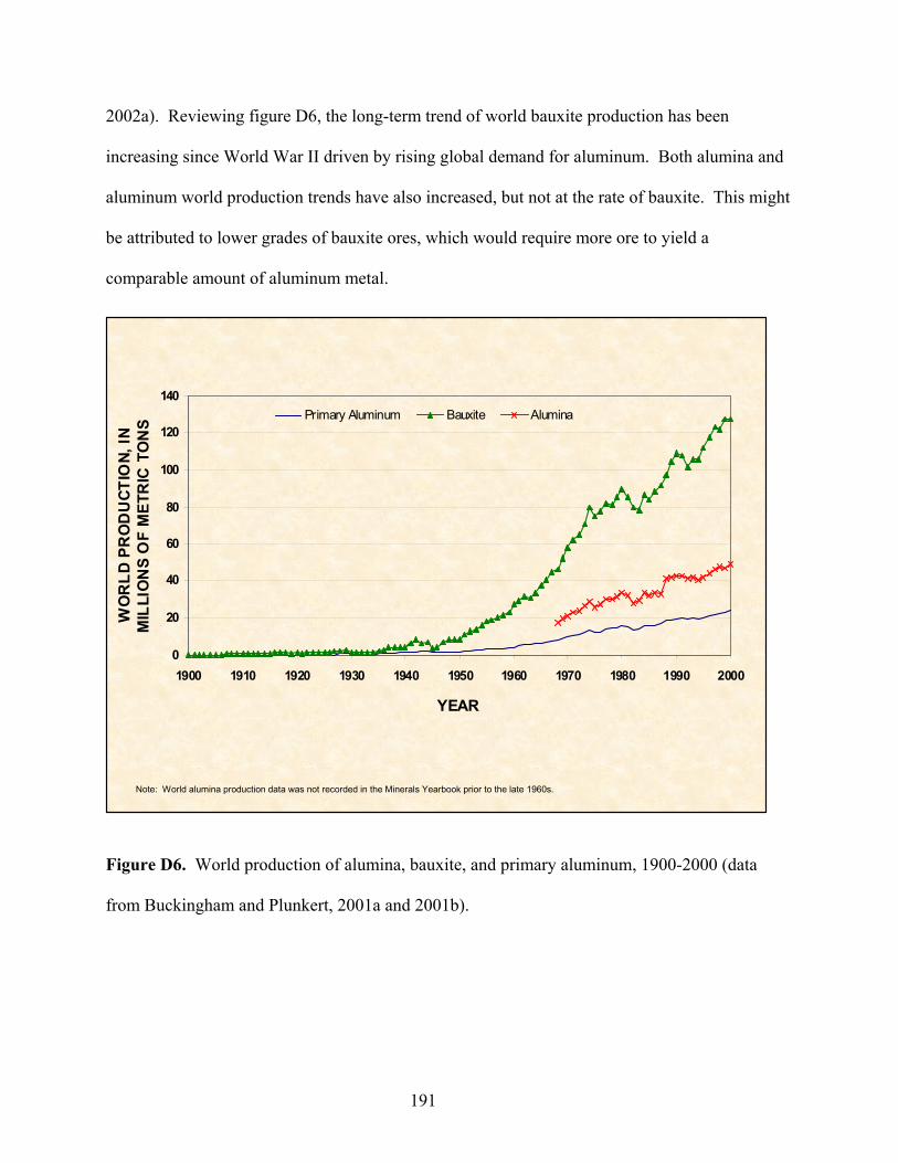
2002a). Reviewing figure D6, the long-term trend of world bauxite production has been
increasing since World War II driven by rising global demand for aluminum. Both alumina and
aluminum world production trends have also increased, but not at the rate of bauxite. This might
be attributed to lower grades of bauxite ores, which would require more ore to yield a
comparable amount of aluminum metal.
0
20
40
60
80
100
120
140
1900 1910 1920 1930 1940 1950 1960 1970 1980 1990 2000
YEAR
WO
RLD
PR
OD
UCT
ION,
IN
MIL
LIO
NS
OF
MET
RIC
TO
NS Primary Aluminum Bauxite Alumina
Note: World alumina production data was not recorded in the Minerals Yearbook prior to the late 1960s.
Figure D6. World production of alumina, bauxite, and primary aluminum, 1900-2000 (data
from Buckingham and Plunkert, 2001a and 2001b).
191
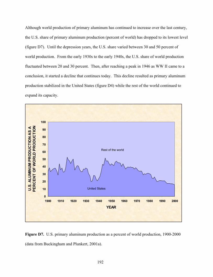
Although world production of primary aluminum has continued to increase over the last century,
the U.S. share of primary aluminum production (percent of world) has dropped to its lowest level
(figure D7). Until the depression years, the U.S. share varied between 30 and 50 percent of
world production. From the early 1930s to the early 1940s, the U.S. share of world production
fluctuated between 20 and 30 percent. Then, after reaching a peak in 1946 as WW II came to a
conclusion, it started a decline that continues today. This decline resulted as primary aluminum
production stabilized in the United States (figure D4) while the rest of the world continued to
expand its capacity.
0
10
20
30
40
50
60
70
80
90
100
1900 1910 1920 1930 1940 1950 1960 1970 1980 1990 2000
YEAR
U.S
. ALU
MIN
UM P
RO
DU
CTI
ON
AS
A PE
RC
ENT
OF
WO
RLD
PR
OD
UCTI
ON
United States
Rest of the world
Figure D7. U.S. primary aluminum production as a percent of world production, 1900-2000
(data from Buckingham and Plunkert, 2001a).
192
Reserves/resources
Worldwide bauxite resources are extensive and the known quantity may increase in the future as
a result of exploration activities. Commercially, bauxite ore is the only raw material used to
produce domestic metallurgical grade alumina. The three largest import sources of bauxite are
Guinea, Australia, and Brazil. Their reported reserve base21 makes up 60 percent of the world
total and is listed in table D1 for 1980, 1990, and 2000.
There is continuing research to develop technology that will economically produce alumina from
other sources such as various clays, coal wastes, and oil shales (U.S. Geological Survey, 2001b,
pg. 29). To date, however, it has been cheaper to import foreign bauxite than to process
domestic nonbauxite resources. Alunite, KAl3 (SO4)2 (OH)6, is a source for alumina, but no
commercial cost-effective process currently exists in the United States to exploit this source.
Alunite deposits are worldwide, with large identified resources in China, Australia, Mexico, and
the former Soviet Union (Hall, 1978). Potential domestic nonbauxite aluminum resources are
abundant and could meet domestic aluminum demand if an economically profitable technology
is developed. It should be noted that the current world reserve base for bauxite is sufficient to
193
21The reserve base is the in-place demonstrated (measured plus indicated) resource from which reserves are estimated.
Alunite was utilized at alumina refineries in the former Soviet Union, but became uneconomical in the post-Soviet era (Casey, 2000). In 2000, a Dutch firm had won a management contract for Azerbaijan’s aluminum holding company and the government expected this new management to restart the Gyandja refinery using alunite ore to produce alumina (Metal Bulletin, 2000).
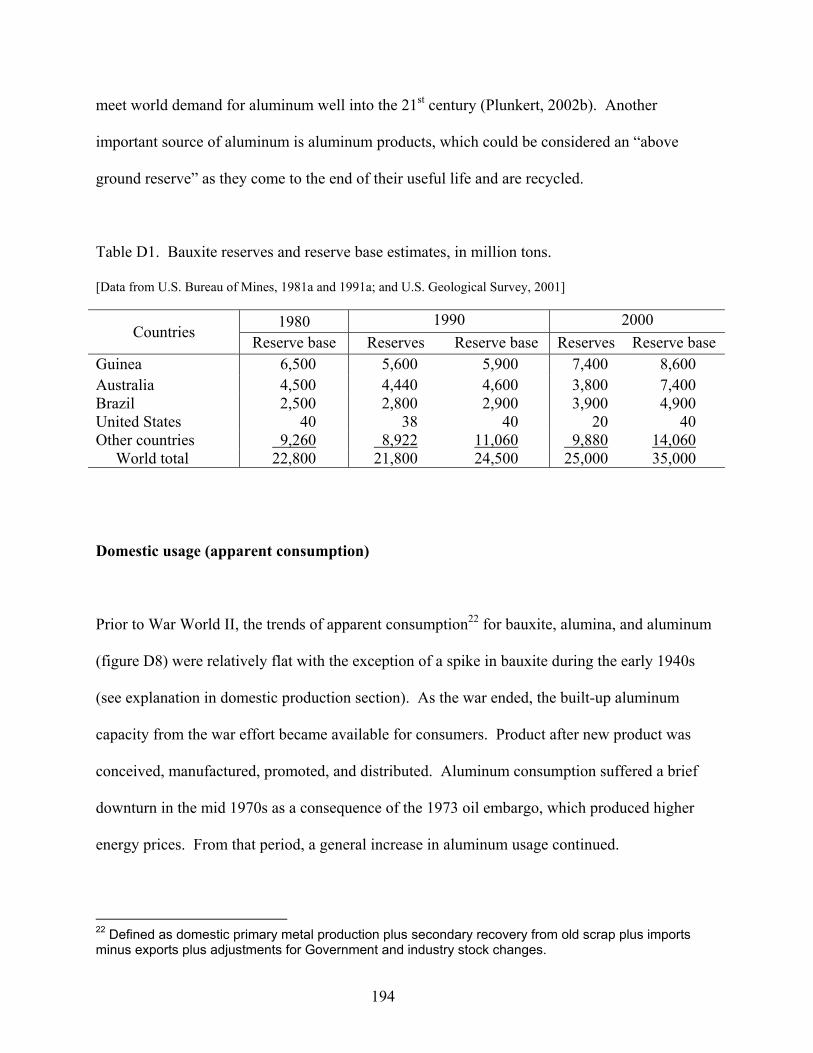
meet world demand for aluminum well into the 21st century (Plunkert, 2002b). Another
important source of aluminum is aluminum products, which could be considered an “above
ground reserve” as they come to the end of their useful life and are recycled.
Table D1. Bauxite reserves and reserve base estimates, in million tons.
[Data from U.S. Bureau of Mines, 1981a and 1991a; and U.S. Geological Survey, 2001]
1980 1990 2000 Countries Reserve base Reserves Reserve base Reserves Reserve base
Guinea 6,500 5,600 5,900 7,400 8,600 Australia 4,500 4,440 4,600 3,800 7,400 Brazil 2,500 2,800 2,900 3,900 4,900 United States 40 38 40 20 40 Other countries 9,260 8,922 11,060 9,880 14,060 World total 22,800 21,800 24,500 25,000 35,000
Domestic usage (apparent consumption)
Prior to War World II, the trends of apparent consumption22 for bauxite, alumina, and aluminum
(figure D8) were relatively flat with the exception of a spike in bauxite during the early 1940s
(see explanation in domestic production section). As the war ended, the built-up aluminum
capacity from the war effort became available for consumers. Product after new product was
conceived, manufactured, promoted, and distributed. Aluminum consumption suffered a brief
downturn in the mid 1970s as a consequence of the 1973 oil embargo, which produced higher
energy prices. From that period, a general increase in aluminum usage continued.
22 Defined as domestic primary metal production plus secondary recovery from old scrap plus imports minus exports plus adjustments for Government and industry stock changes.
194
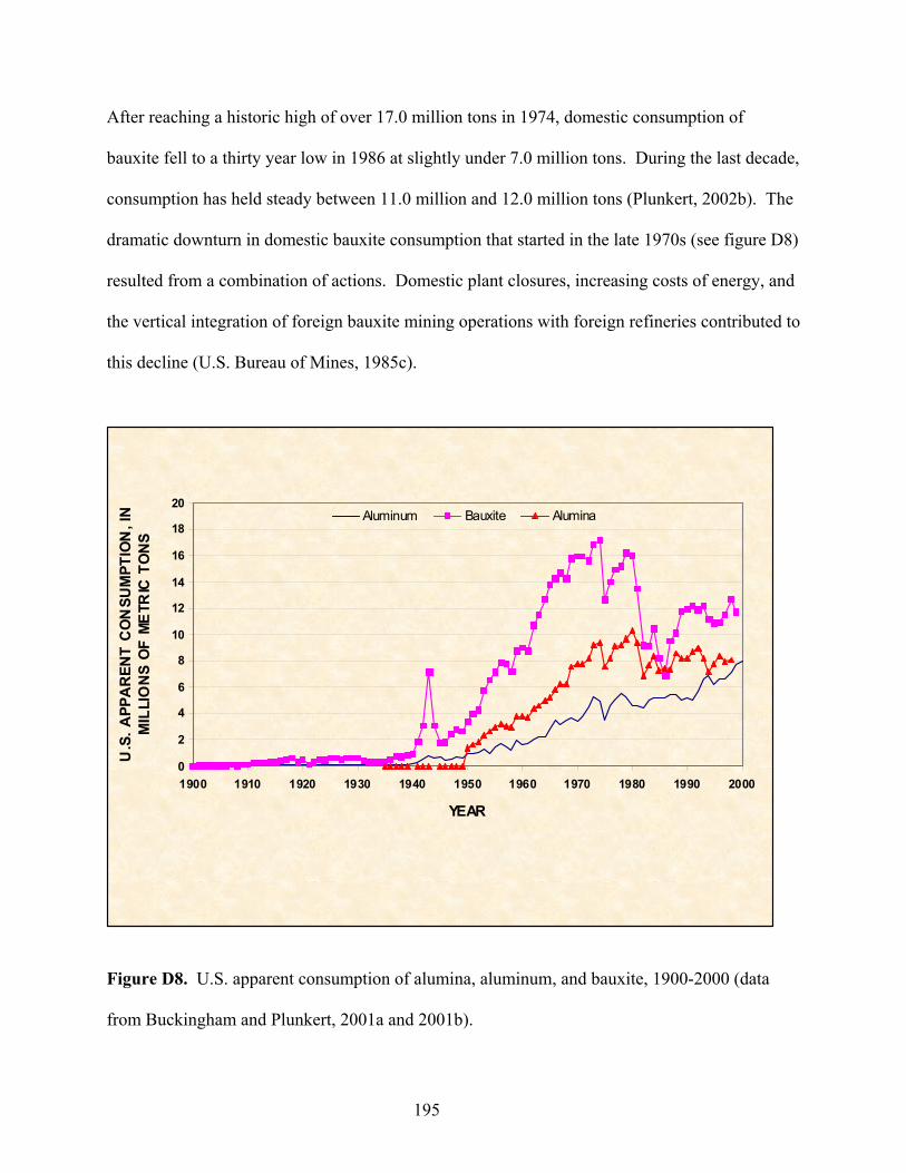
After reaching a historic high of over 17.0 million tons in 1974, domestic consumption of
bauxite fell to a thirty year low in 1986 at slightly under 7.0 million tons. During the last decade,
consumption has held steady between 11.0 million and 12.0 million tons (Plunkert, 2002b). The
dramatic downturn in domestic bauxite consumption that started in the late 1970s (see figure D8)
resulted from a combination of actions. Domestic plant closures, increasing costs of energy, and
the vertical integration of foreign bauxite mining operations with foreign refineries contributed to
this decline (U.S. Bureau of Mines, 1985c).
0
2
4
6
8
10
12
14
16
18
20
1900 1910 1920 1930 1940 1950 1960 1970 1980 1990 2000
YEAR
U.S
. APP
AR
ENT
CO
NSU
MPT
ION
, IN
M
ILLI
ON
S O
F M
ETR
IC T
ON
S
Aluminum Bauxite Alumina
Figure D8. U.S. apparent consumption of alumina, aluminum, and bauxite, 1900-2000 (data
from Buckingham and Plunkert, 2001a and 2001b).
195
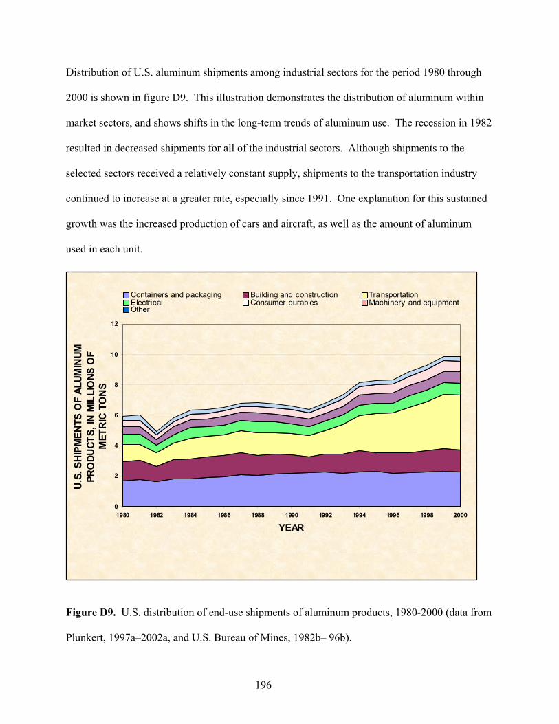
Distribution of U.S. aluminum shipments among industrial sectors for the period 1980 through
2000 is shown in figure D9. This illustration demonstrates the distribution of aluminum within
market sectors, and shows shifts in the long-term trends of aluminum use. The recession in 1982
resulted in decreased shipments for all of the industrial sectors. Although shipments to the
selected sectors received a relatively constant supply, shipments to the transportation industry
continued to increase at a greater rate, especially since 1991. One explanation for this sustained
growth was the increased production of cars and aircraft, as well as the amount of aluminum
used in each unit.
0
2
4
6
8
10
12
1980 1982 1984 1986 1988 1990 1992 1994 1996 1998 2000
YEAR
U.S
. SH
IPM
ENTS
OF
ALUM
INUM
PR
ODU
CTS,
IN M
ILLI
ONS
OF
MET
RIC
TO
NS
Containers and packaging Building and construction TransportationElectrical Consumer durables Machinery and equipmentOther
Figure D9. U.S. distribution of end-use shipments of aluminum products, 1980-2000 (data from
Plunkert, 1997a–2002a, and U.S. Bureau of Mines, 1982b– 96b).
196
Globalization
Most of the restructuring of the world aluminum industry began in the late 1970s as the cost of
energy soared due to higher oil prices. Bauxite mining operations with access to cheaper forms
of power, for example, hydroelectric, built alumina refineries and aluminum smelters. Today,
Australia and China have emerged as major primary aluminum producers. Canada continues to
provide the bulk of aluminum imports to the United States, which amounted to 55 percent in
2000 (Plunkert, 2002a). Other countries that are key producers of aluminum in order of
decreasing production are Russia, Brazil, and Norway.
The primary source for aluminum is the metallurgical-grade of bauxite ore, which is distributed
unequally around the globe. Initially, bauxite-producing countries operated their mining
operations with no facilities downstream in the production process. If possible, they eventually
moved into higher value processing by producing alumina or aluminum metal. As international
demand for aluminum and associated products increased, the development of mining and
processing operations spread worldwide.
The United States is heavily reliant on imports for metallurgical-grade bauxite that is used for the
production of alumina from which the metal aluminum is produced. In the early 1990s, it was
estimated that approximately 90 percent of the bauxite mine output in market economy countries
was for metallurgical use (Wilburn and Wagner, 1993). Minor amounts of nonmetallugical
grade bauxite are exported to be used in products such as abrasives, chemicals, and refractories.
Reviewing figure D10, bauxite imports, after peaking in 1974 at 15.5 million tons, turned down
197
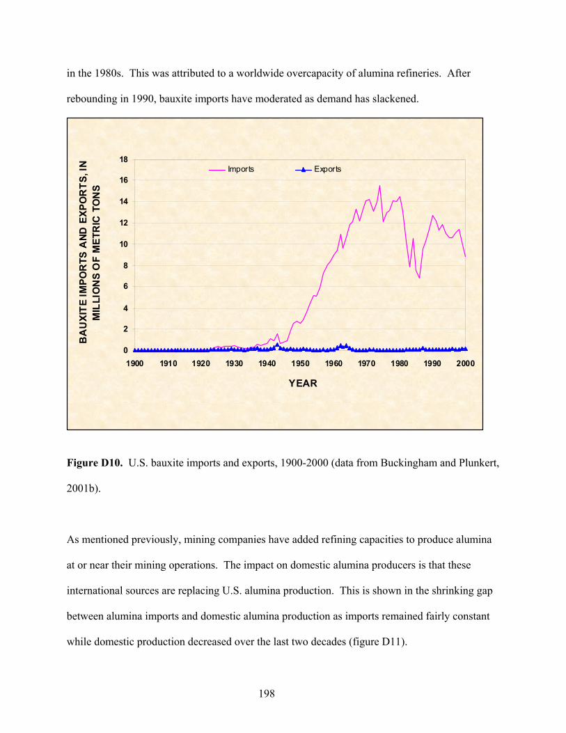
in the 1980s. This was attributed to a worldwide overcapacity of alumina refineries. After
rebounding in 1990, bauxite imports have moderated as demand has slackened.
0
2
4
6
8
10
12
14
16
18
1900 1910 1920 1930 1940 1950 1960 1970 1980 1990 2000
YEAR
BA
UXI
TE IM
POR
TS A
ND E
XPO
RTS
, IN
M
ILLI
ON
S O
F M
ETR
IC T
ON
S
Imports Exports
Figure D10. U.S. bauxite imports and exports, 1900-2000 (data from Buckingham and Plunkert,
2001b).
As mentioned previously, mining companies have added refining capacities to produce alumina
at or near their mining operations. The impact on domestic alumina producers is that these
international sources are replacing U.S. alumina production. This is shown in the shrinking gap
between alumina imports and domestic alumina production as imports remained fairly constant
while domestic production decreased over the last two decades (figure D11).
198

0
1
2
3
4
5
6
7
8
1930 1940 1950 1960 1970 1980 1990 2000
YEAR
U.S
. ALU
MIN
A IM
POR
TS, E
XPO
RTS,
AN
D PR
OD
UCTI
ON,
IN M
ILLI
ON
SO
F M
ETRI
C TO
NSImports Exports Production
Figure D11. U.S. alumina imports, exports, and production, 1935-2000 (data from Buckingham
and Plunkert, 2001b).
Aluminum imports and exports quantities were approximately equal until the early 1990s when
they diverged with imports rising sharply (figure D12). This trend will probably continue as the
domestic aluminum industry depends more on aluminum imports due in part to higher energy
prices and stricter environmental regulations.
199
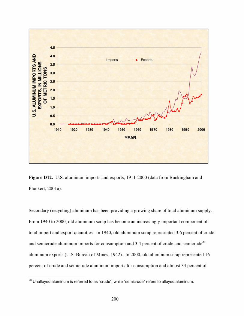
0.0
0.5
1.0
1.5
2.0
2.5
3.0
3.5
4.0
4.5
1910 1920 1930 1940 1950 1960 1970 1980 1990 2000
YEAR
U.S
. ALU
MIN
UM
IMPO
RTS
AND
EXPO
RTS,
IN M
ILLI
ONS
OF
MET
RIC
TO
NS
Imports Exports
Figure D12. U.S. aluminum imports and exports, 1911-2000 (data from Buckingham and
Plunkert, 2001a).
Secondary (recycling) aluminum has been providing a growing share of total aluminum supply.
From 1940 to 2000, old aluminum scrap has become an increasingly important component of
total import and export quantities. In 1940, old aluminum scrap represented 3.6 percent of crude
and semicrude aluminum imports for consumption and 3.4 percent of crude and semicrude23
aluminum exports (U.S. Bureau of Mines, 1942). In 2000, old aluminum scrap represented 16
percent of crude and semicrude aluminum imports for consumption and almost 33 percent of
200
23 Unalloyed aluminum is referred to as “crude”, while “semicrude” refers to alloyed aluminum.
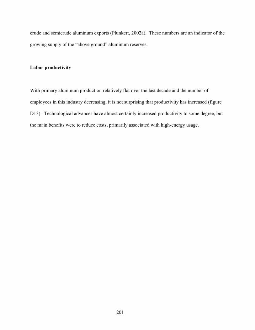
crude and semicrude aluminum exports (Plunkert, 2002a). These numbers are an indicator of the
growing supply of the “above ground” aluminum reserves.
Labor productivity
With primary aluminum production relatively flat over the last decade and the number of
employees in this industry decreasing, it is not surprising that productivity has increased (figure
D13). Technological advances have almost certainly increased productivity to some degree, but
the main benefits were to reduce costs, primarily associated with high-energy usage.
201
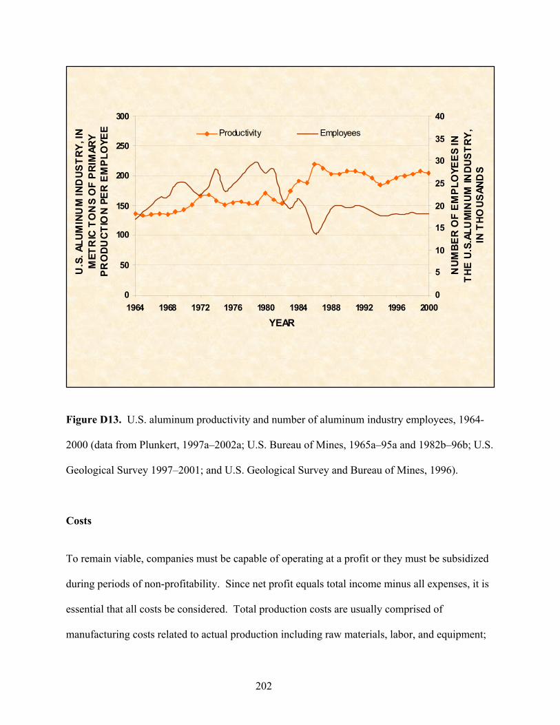
0
50
100
150
200
250
300
1964 1968 1972 1976 1980 1984 1988 1992 1996 2000YEAR
U.S
. ALU
MIN
UM
IND
USTR
Y, IN
M
ETR
IC T
ON
S O
F PR
IMAR
Y PR
ODU
CTIO
N PE
R E
MPL
OYE
E
0
5
10
15
20
25
30
35
40
NUM
BER
OF
EMPL
OYE
ES IN
TH
E U.
S.AL
UM
INUM
INDU
STRY
, IN
THO
USAN
DS
Productivity Employees
Figure D13. U.S. aluminum productivity and number of aluminum industry employees, 1964-
2000 (data from Plunkert, 1997a–2002a; U.S. Bureau of Mines, 1965a–95a and 1982b–96b; U.S.
Geological Survey 1997–2001; and U.S. Geological Survey and Bureau of Mines, 1996).
Costs
To remain viable, companies must be capable of operating at a profit or they must be subsidized
during periods of non-profitability. Since net profit equals total income minus all expenses, it is
essential that all costs be considered. Total production costs are usually comprised of
manufacturing costs related to actual production including raw materials, labor, and equipment;
202

and general expenses such as administrative salaries, product distribution costs, research and
development, and taxes. Although individual companies typically report these costs in their
annual reports, a broader measure is available through the U.S. Census Bureau’s publication,
Economic Census – Manufacturing, (1999).
Table D2 contains 1992 and 1997 primary aluminum industry data from the U.S. Census Bureau
(1999). The right-hand column in the table lists the percent changes from 1992 to 1997. All the
categories in the primary aluminum industry had decreases from 1992 to 1997. In both
compensation categories, “all employee payroll” and “production worker wages” decreases of 23
and 26 percent respectively were noted in terms of 2000 dollars. All of these changes were the
effects of continuing technological process improvements and consolidation in this industry.
Table D2. Domestic primary aluminum industry data.
[Adapted from Bureau of Census, 1995 and U.S. Census Bureau, 1999; —, not applicable]
Category 1992 1997 Change, in percent
Quantity 2000 constant dollars
Quantity 2000 constant dollars
Companies 30 — 13 — -56.7 Number of employees 20,400 — 15,763 — -22.7 Wages of employees — 981,249,000 — 752,956,000 -23.3
16,200 — 12,624 — -22.1 Wages of production workers — 739,924,000 — 545,972,000 -26.2 Cost of materials — — 3,946,175,000 -23.3 5,147,596,000
-28.0 Product shipments – tons 4,689,377 — 4,074,390 — -13.1
Number of production workers
Electricity purchased in kilowatt-hours
60,272,400,000
—
43,426,337,000
—
203
Supply/demand
Aluminum applications continue to expand in areas ranging from automobiles to housing and
infrastructure. Technological advancements have also helped to make aluminum products more
cost competitive. All of these factors have been driving up aluminum demand.
The domestic demand for aluminum is growing in many industries, with 2000 shipments of 11.1
million tons. The transportation industry was the largest consumer of aluminum, receiving 2000
shipments of 3.61 million tons. As stated in the Ducker Report, the American passenger car
contained an average of 241 pounds of aluminum in 1999. This is an increase of 23 kilograms
(50 pounds) over 1991 (Ducker Research Company, Inc., 1998§). The second largest consumer
of aluminum was the domestic container and packaging industry, which used over 2.26 million
tons in 2000. The Can Manufacturers Institute, Inc. (2001§) reported that over 100 billion
aluminum beverage cans were shipped in 2000. Based on an average of 73 cans per kilogram
(33 cans per pound), this equals approximately 1.4 million tons. The 2000 U.S. apparent
supply inum, reported by the U.S. Geological Survey was 9.61 million tons. Primary
domestic production was 3.67 million tons with secondary production (recycled) at 3.45 million
tons. Recycled aluminum supplied slightly less than half of the total U.S. production in 2000.
Imports for consumption were 3.91 million tons and exports were listed as 1.76 million tons
(Plunkert, 2002a).
24 of alum
24 Defined as domestic primary metal production plus secondary recovery plus imports minus exports plus adjustments for Government and industry stocks changes.
204
Demand for aluminum products is anticipated to grow, as developing nations expand their
transportation industry, primarily in the automobile and aircraft sectors. Likewise, world
production is expected to continue to rise, meeting this demand as new international facilities
associated with bauxite mining companies come into the production stream.
Conclusions
The aluminum industry was born during the Industrial Revolution. In the early 1900s, aluminum
was in high demand for both railroad cars and automobiles due to aluminum’s desirable
properties (lightweight and high strength). Production was stimulated again during World War II
to meet the wartime demand for aluminum, which was especially critical to military aircraft.
During the 1950s and 1960s, the excess production capacity was used for numerous new
aluminum applications. As a growing number of Americans became more conscious of
protecting the environment in the 1970s, recycling aluminum cans became a widespread
industrial activity in the United States. Also, an economic incentive was provided as recycled
centers exchanged money for aluminum cans. Secondary scrap has assumed a major portion of
the domestic aluminum supply. In 2000, aluminum recovered from new and old scrap reached
3.45 million tons. Today, almost half the supply of aluminum metal in the United States
originates from recycling (all aluminum products).
The international aluminum supply has met the increased demand as worldwide production
capacity continues its expansion with the construction of new refineries and smelters. The
growth of aluminum consumption reflects the widespread applications of this metal in global
205

industries such as building and construction, containers and packaging, and transportation.
Aluminum-based materials are heavily traded internationally, which demonstrate the global
nature of the aluminum industry.
206
References
Banks, A.J., 1992, What’s the use? in Journal of Chemical Education, January 1992, v. 69, p. 18. Buckingham, D.A., and Plunkert, P.A., 2001a, Aluminum statistics, in Historical statistics for mineral commodities in the United States: U.S. Geological Survey Open-File Report 01-006.
U.S. Census Bureau, 1999, 1997 Economic census- Manufacturing: U.S. Census Bureau, EC97M-3313B, 29 p.
Buckingham, D.A., and Plunkert, P.A., 2001b, Bauxite and alumina statistics, in Historical statistics for mineral commodities in the United States: U.S. Geological Survey Open-File Report 01-006. Bureau of the Census, 1995, 1992 Census of manufacturers—Smelting and refining of nonferrous metals and alloys: Bureau of the Census, MC92-1-33C, 33 p. Casey, Simon, 2000, Russia’s aluminum industry focuses on securing raw materials, in Metal Bulletin, no. 8497, July 31, 2000, p. 5. Hall, R. B., 1978, World nonbauxite aluminum resources – Alunite: U.S. Geological Survey Professional Paper 1076-A, 30 p. Metal Bulletin, 2000, Dutch firm gets Azeraluminy management contract: Metal Bulletin, No. 8517, October 16, 2000, p. 3. Plunkert, P. A., 1997a-2002a, Aluminum, in Metals and Minerals: U.S. Geological Survey Minerals Yearbook 1995-2000. Plunkert, P. A., 2002b, Bauxite and alumina, in Metals and Minerals: U.S. Geological Survey Minerals Yearbook 2000, v. I, p. 11.1-11.12.
U.S. Bureau of Mines, 1942-43, Aluminum, in Metals and Minerals: U.S. Bureau of Mines Minerals Yearbook 1941-42, v. I. U.S. Bureau of Mines, 1965a-95a, Mineral commodity summaries 1965-95: U.S. Bureau of Mines. U.S. Bureau of Mines, 1982b-96b, Aluminum, in Metals and Minerals: U.S. Bureau of Mines Minerals Yearbook 1981-94, v. I. U.S. Bureau of Mines, 1985c, Mineral Facts and Problems, 1985 edition: U.S. Bureau of Mines Bulletin 675, 956 p.
207
U.S. Geological Survey, 1902, Mineral resources of the United States 1901: U.S. Geological Survey, 996 p. U.S. Geological Survey, 1997-2001, Mineral commodity summaries 1997-2001: U.S. Geological Survey. U.S. Geological Survey and Bureau of Mines, 1996, Mineral commodity summaries, 1996: U.S. Geological Survey and U.S. Bureau of Mines, 195 p. Wilburn, D.R., and Wagner, L.A., 1993, Aluminum availability and supply – A minerals availability appraisal: U.S. Bureau of Mines Information Circular 9371, 140 p. Internet references cited The Can Manufacturers Institute, Inc., 2001, Aluminum beverage can shipments report, accessed July 19, 2002, at URL http://www.cancentral.com/stats.cfm. Ducker Research Company, Inc., 1998, 1999 Passenger and light truck aluminum content report highlights, accessed February 2, 2001, at URL http://www.autoaluminum.org/miscpdfs/press_stats.pdf. International Aluminium Institute, 2001, Current IAI statistics, accessed June 21, 2001 at URL http://www.world-aluminium.org/iai/stats/750.html.
208
APPENDIX E: ECONOMIC CASE STUDY -- COPPER
Introduction/background
Copper was one of the first metals to be utilized for tools, weapons, and ornaments. Copper has
many useful physical properties such as high electrical and thermal conductivity, corrosion
resistance, ductility and malleability, and high strength. It is also nonmagnetic. The multitude of
electrical-based inventions that followed the discovery of electricity greatly expanded the uses
for copper. Copper is used in electrical and telecommunications products, building construction,
industrial machinery and equipment, transportation, and consumer products.
Historical economic trends
The price of copper, in constant 2000 dollars, is shown in Figure E1 for the period from 1900
through 2000. The figure shows that the price is highly volatile with an overall downward trend
for the period. During World War I, the price reached more than $4 per pound in 2000 dollars
because of the increased demand for copper in munitions and other aspects of the war effort. In
1932, in the midst of the Great Depression, the price bottomed out at $0.73 per pound (2000
dollars). During World War II, the price was controlled by the government but rose again during
the postwar boom to a high of $2.64 in 1956 (2000 dollars). After declining because of a
recession, the price began a gradual increase until 1971 when price controls were used to fight
inflation. After controls were ended, the price rose again reaching a peak of $2.67 per pound in
1974 (2000 dollars). Since that time, the price has generally declined with a trough during the
recession of the 1980s. Copper prices in the late 1990s (2000 dollars) approached the all time
209

historic low that had occurred during the Great Depression. The volatility, not explained by
major economic and political events, resulted from technological innovations and changes in the
copper market. Because the copper industry is made up of a small number of large producers,
operations opening or closing have a large impact on supply. This results in volatile prices.
0.00
1.00
2.00
3.00
4.00
5.00
6.00
1900 1910 1920 1930 1940 1950 1960 1970 1980 1990 2000
YEAR
U.S.
CO
PPER
PR
ICE
IN C
ONS
TANT
200
0 D
OLL
ARS
PER
PO
UND
Price Linear trendWorld War I
World War II
Great Depression
Oil crisis
Recession
Figure E1. U.S. copper price, in constant 2000 dollars, 1900-2000 (data from Porter and
Edelstein, 2001).
U.S. mine production of copper is shown in figure E2. The figure shows that production from
year to year was volatile although with an overall increasing trend. Rising production in
conjunction with declining prices is not inconsistent with traditional supply and demand theory.
210
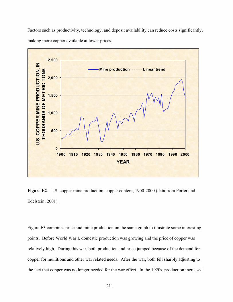
Factors such as productivity, technology, and deposit availability can reduce costs significantly,
making more copper available at lower prices.
0
500
1,000
1,500
2,000
2,500
1900 1910 1920 1930 1940 1950 1960 1970 1980 1990 2000
YEAR
U.S.
CO
PPER
MIN
E PR
OD
UCTI
ON,
IN
THO
USAN
DS
OF
MET
RIC
TO
NS
Mine production Linear trend
Figure E2. U.S. copper mine production, copper content, 1900-2000 (data from Porter and
Edelstein, 2001).
Figure E3 combines price and mine production on the same graph to illustrate some interesting
points. Before World War I, domestic production was growing and the price of copper was
relatively high. During this war, both production and price jumped because of the demand for
copper for munitions and other war related needs. After the war, both fell sharply adjusting to
the fact that copper was no longer needed for the war effort. In the 1920s, production increased
211
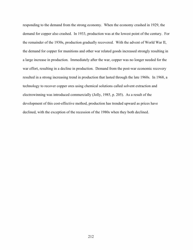
responding to the demand from the strong economy. When the economy crashed in 1929, the
demand for copper also crashed. In 1933, production was at the lowest point of the century. For
the remainder of the 1930s, production gradually recovered. With the advent of World War II,
the demand for copper for munitions and other war related goods increased strongly resulting in
a large increase in production. Immediately after the war, copper was no longer needed for the
war effort, resulting in a decline in production. Demand from the post-war economic recovery
resulted in a strong increasing trend in production that lasted through the late 1960s. In 1968, a
technology to recover copper ores using chemical solutions called solvent extraction and
electrowinning was introduced commercially (Jolly, 1985, p. 205). As a result of the
development of this cost-effective method, production has trended upward as prices have
declined, with the exception of the recession of the 1980s when they both declined.
212
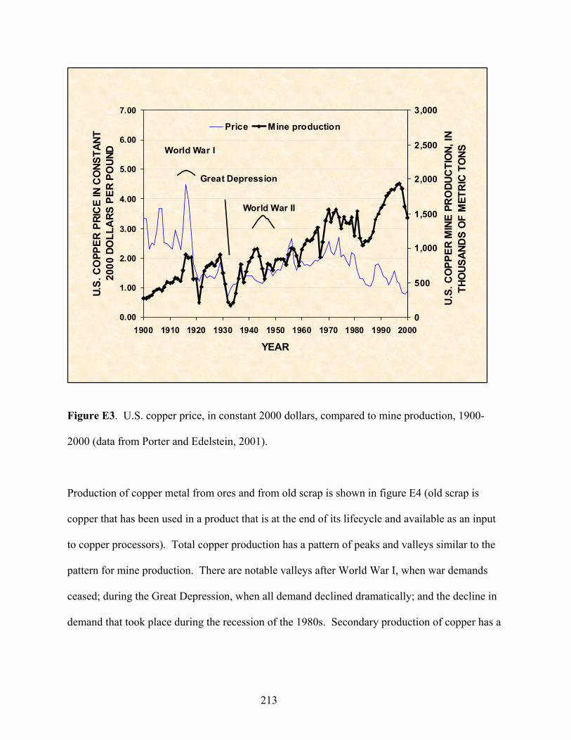
0.00
1.00
2.00
3.00
4.00
5.00
6.00
7.00
1900 1910 1920 1930 1940 1950 1960 1970 1980 1990 2000
YEAR
U.S.
CO
PPER
PRI
CE
IN C
ONS
TANT
20
00 D
OLL
ARS
PER
PO
UND
0
500
1,000
1,500
2,000
2,500
3,000
U.S.
CO
PPER
MIN
E PR
ODU
CTI
ON,
IN
THO
USAN
DS
OF
MET
RIC
TO
NS
Price Mine production
World War I
Great Depression
World War II
Figure E3. U.S. copper price, in constant 2000 dollars, compared to mine production, 1900-
2000 (data from Porter and Edelstein, 2001).
Production of copper metal from ores and from old scrap is shown in figure E4 (old scrap is
copper that has been used in a product that is at the end of its lifecycle and available as an input
to copper processors). Total copper production has a pattern of peaks and valleys similar to the
pattern for mine production. There are notable valleys after World War I, when war demands
ceased; during the Great Depression, when all demand declined dramatically; and the decline in
demand that took place during the recession of the 1980s. Secondary production of copper has a
213
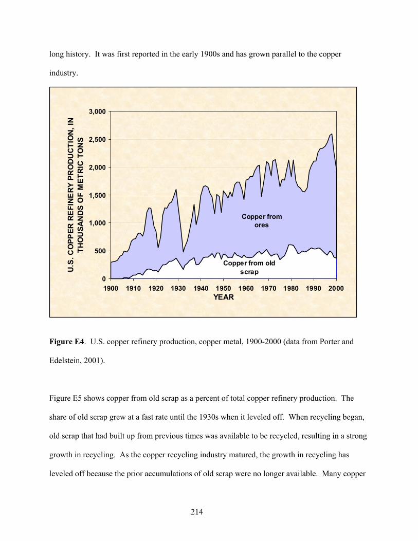
long history. It was first reported in the early 1900s and has grown parallel to the copper
industry.
Copper from old scrap
Copper from ores
0
500
1,000
1,500
2,000
2,500
3,000
1900 1910 1920 1930 1940 1950 1960 1970 1980 1990 2000YEAR
U.S.
CO
PPER
REF
INER
Y PR
ODU
CTIO
N, IN
TH
OU
SAN
DS O
F M
ETRI
C T
ON
S
Figure E4. U.S. copper refinery production, copper metal, 1900-2000 (data from Porter and
Edelstein, 2001).
Figure E5 shows copper from old scrap as a percent of total copper refinery production. The
share of old scrap grew at a fast rate until the 1930s when it leveled off. When recycling began,
old scrap that had built up from previous times was available to be recycled, resulting in a strong
growth in recycling. As the copper recycling industry matured, the growth in recycling has
leveled off because the prior accumulations of old scrap were no longer available. Many copper
214
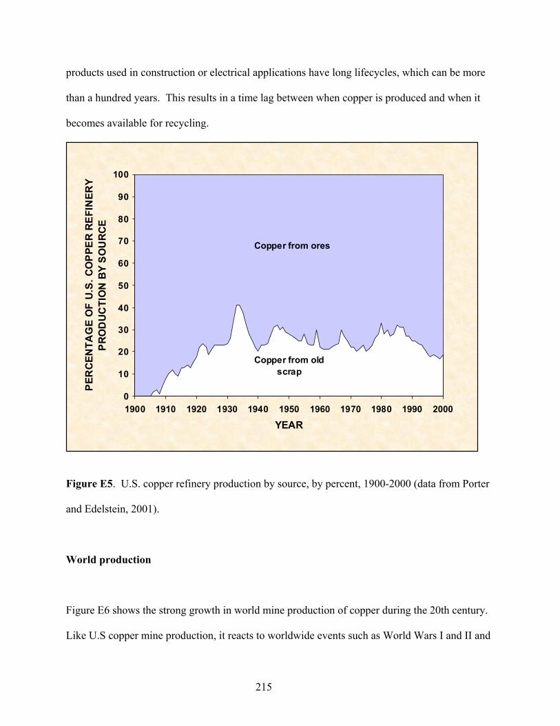
products used in construction or electrical applications have long lifecycles, which can be more
than a hundred years. This results in a time lag between when copper is produced and when it
becomes available for recycling.
Copper from old scrap
0
10
20
30
40
50
60
70
80
90
100
1900 1910 1920 1930 1940 1950 1960 1970 1980 1990 2000YEAR
PER
CEN
TAG
E O
F U.
S. C
OPP
ER R
EFIN
ERY
PRO
DUC
TIO
N B
Y SO
URC
E
Copper from ores
Figure E5. U.S. copper refinery production by source, by percent, 1900-2000 (data from Porter
and Edelstein, 2001).
World production
Figure E6 shows the strong growth in world mine production of copper during the 20th century.
Like U.S copper mine production, it reacts to worldwide events such as World Wars I and II and
215

the worldwide Great Depression. The curve exhibits the characteristics of a compound growth
rate. Comparing 495 thousand tons produced in 1900 to 12.9 million tons produced in 2000, the
annual growth rate was 3.3 percent for this 100-year period.
0
2
4
6
8
10
12
14
1900 1910 1920 1930 1940 1950 1960 1970 1980 1990 2000
YEAR
WO
RLD
CO
PPER
MIN
E PR
ODU
CTIO
N, IN
M
ILLI
ONS
OF
MET
RIC
TO
NS
Figure E6. World copper mine production, copper content, 1900-2000 (data from Porter and
Edelstein, 2001).
Figure E7 shows U.S. copper mine production as a percent of world mine production. It shows
that for most years between 1900 and the Great Depression, U.S. production accounted for more
than 50 percent of total world mine production. During the Depression of the 1930s, the U.S.
share sank below 17 percent. It rose to a high of almost 39 percent during World War II and has
216
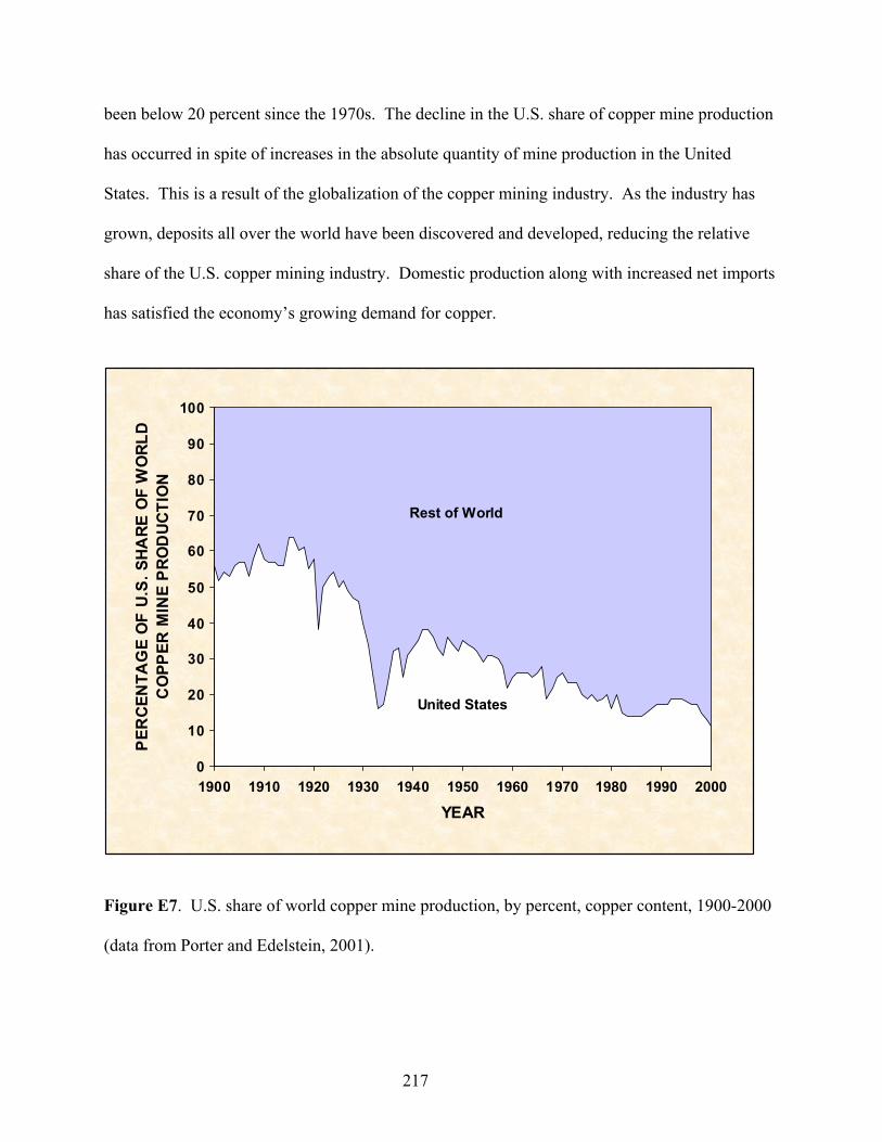
been below 20 percent since the 1970s. The decline in the U.S. share of copper mine production
has occurred in spite of increases in the absolute quantity of mine production in the United
States. This is a result of the globalization of the copper mining industry. As the industry has
grown, deposits all over the world have been discovered and developed, reducing the relative
share of the U.S. copper mining industry. Domestic production along with increased net imports
has satisfied the economy’s growing demand for copper.
United States
0
10
20
30
40
50
60
70
80
90
100
1900 1910 1920 1930 1940 1950 1960 1970 1980 1990 2000
YEAR
PER
CEN
TAG
E O
F U.
S. S
HARE
OF
WO
RLD
CO
PPER
MIN
E PR
OD
UCTI
ON
Rest of World
Figure E7. U.S. share of world copper mine production, by percent, copper content, 1900-2000
(data from Porter and Edelstein, 2001).
217

Reserves/resources
The 2000 world copper reserves were estimated to be 340 million tons of copper content; those
of the United States were 45 million tons, 13 percent of the world total. The world copper
reserve base for 2000 was estimated to be 650 million tons copper content. The 2000 reserve
base for the United States was 90 million tons, almost 14 percent of the world estimate
(Edelstein, 2001, p. 53). As a comparison, the 1981 world reserve base was estimated to be 505
million tons. For the United States, it was 90 million tons, almost 18 percent of the world
estimate (Butterman, 1982, p. 41). The world reserve base increased as copper mining took
place because more material was being added to the reserve base through exploration and
changes in economic conditions than was removed through mining. New developments in
mining and ore processing equipment have greatly increased reserves by making possible the
recovery of copper from ore that was not economically feasible using older technologies
(Wilburn, Goonan, and Bleiwas, 2001). This demonstrates that reserve base and reserves are
dynamic concepts and should not be used as long run indicators of the future availability of the
material.
Use
Copper use in the United States as measured by apparent consumption (fig. E8) has a strong
increasing trend during the 20th century. Fluctuations reflect the economic and political events
of the century. Apparent consumption of copper reached a new high during World War I
because of an increased demand for copper for the war effort. It declined when the war effort
218
ended. Apparent consumption increased again when the economic boom of the 1920s caused the
demand for copper to increase. Demand dropped for most copper products during the Great
Depression, resulting in the fall of copper apparent consumption. The war effort during World
War II caused a strong demand for copper and large growth in apparent consumption. With the
end of the war, copper apparent consumption declined, but remained much higher than before the
war. Copper demand and apparent consumption increased during the post-war economic boom.
The economic growth continued through 1998, with interruptions caused by the oil crisis of the
1970s and the recession of the 1980s. The reason copper demand follows the economy is
because it is used in industries whose markets are integral parts of the economy. In the United
States in 2000, 41 percent of copper was used in building construction, 27 percent was used in
electrical and electronic products, 12 percent was used in transportation equipment, 10 percent in
industrial machinery and equipment, and 10 percent in consumer and general products
(Edelstein, 2001, p. 52).
219
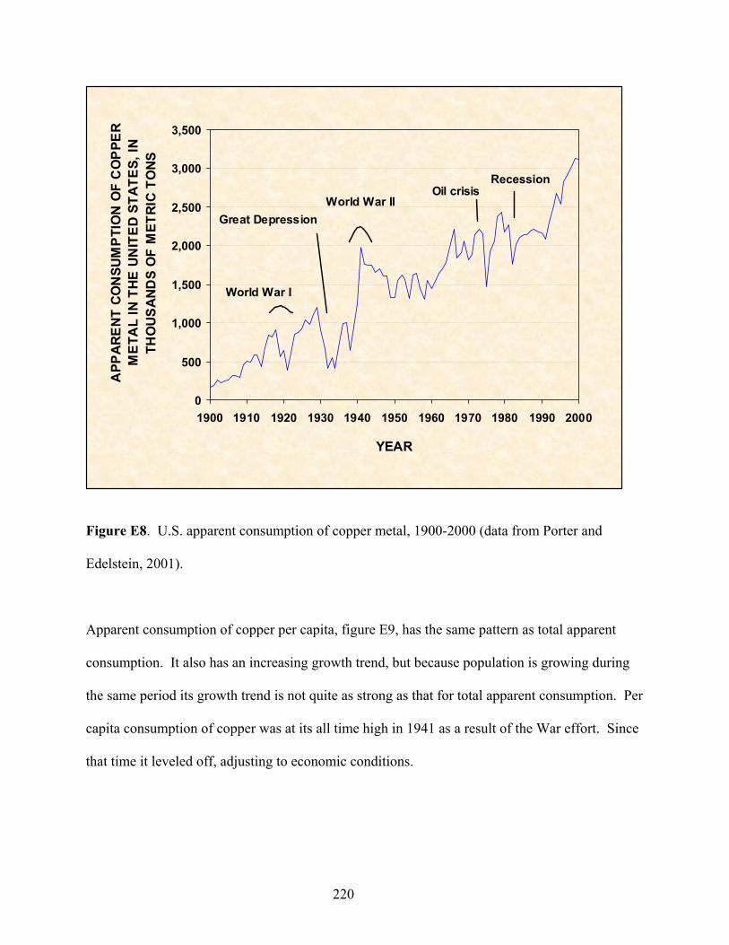
0
500
1,000
1,500
2,000
2,500
3,000
3,500
1900 1910 1920 1930 1940 1950 1960 1970 1980 1990 2000
YEAR
APP
AREN
T CO
NSU
MPT
ION
OF
CO
PPER
M
ETA
L IN
THE
UN
ITED
STA
TES,
IN
THO
USAN
DS
OF
MET
RIC
TONS
World War I
Great DepressionWorld War II
Oil crisisRecession
Figure E8. U.S. apparent consumption of copper metal, 1900-2000 (data from Porter and
Edelstein, 2001).
Apparent consumption of copper per capita, figure E9, has the same pattern as total apparent
consumption. It also has an increasing growth trend, but because population is growing during
the same period its growth trend is not quite as strong as that for total apparent consumption. Per
capita consumption of copper was at its all time high in 1941 as a result of the War effort. Since
that time it leveled off, adjusting to economic conditions.
220
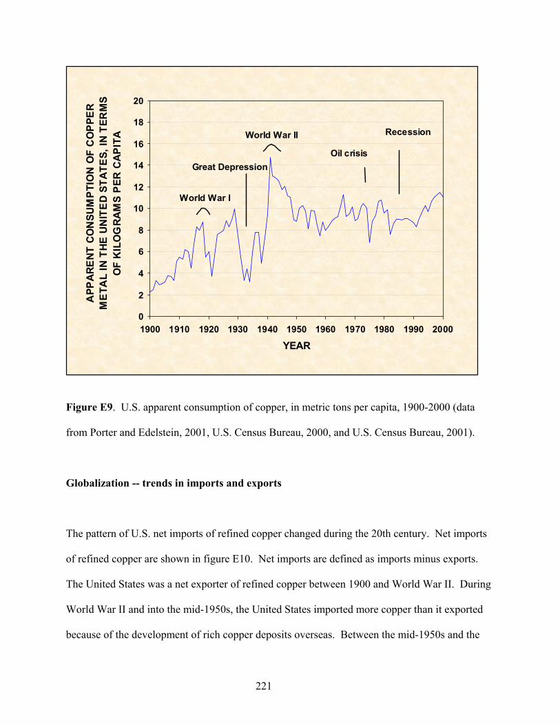
0
2
4
6
8
10
12
14
16
18
20
1900 1910 1920 1930 1940 1950 1960 1970 1980 1990 2000
YEAR
APP
AREN
T CO
NSU
MPT
ION
OF
CO
PPER
M
ETA
L IN
THE
UN
ITED
STA
TES,
IN T
ERM
S O
F K
ILO
GRA
MS
PER
CAP
ITA
World War I
Great Depression
World War II
Oil crisis
Recession
Figure E9. U.S. apparent consumption of copper, in metric tons per capita, 1900-2000 (data
from Porter and Edelstein, 2001, U.S. Census Bureau, 2000, and U.S. Census Bureau, 2001).
Globalization -- trends in imports and exports
The pattern of U.S. net imports of refined copper changed during the 20th century. Net imports
of refined copper are shown in figure E10. Net imports are defined as imports minus exports.
The United States was a net exporter of refined copper between 1900 and World War II. During
World War II and into the mid-1950s, the United States imported more copper than it exported
because of the development of rich copper deposits overseas. Between the mid-1950s and the
221
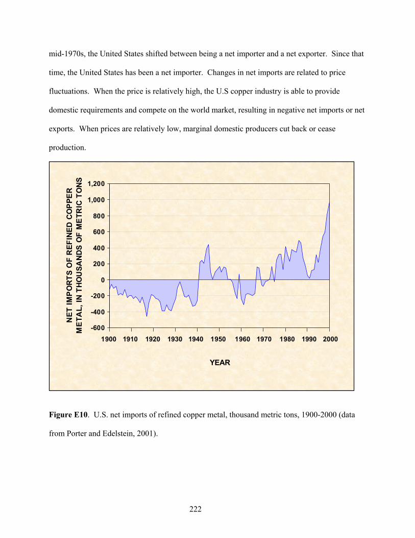
222
mid-1970s, the United States shifted between being a net importer and a net exporter. Since that
time, the United States has been a net importer. Changes in net imports are related to price
fluctuations. When the price is relatively high, the U.S copper industry is able to provide
domestic requirements and compete on the world market, resulting in negative net imports or net
exports. When prices are relatively low, marginal domestic producers cut back or cease
production.
-600
-400
-200
0
200
400
600
800
1,000
1,200
YEAR
NET
IMPO
RTS
OF
REF
INED
CO
PPER
M
ETA
L, IN
THO
USA
NDS
OF
MET
RIC
TO
NS
1900 1910 1920 1940 1950 1960 1970 1980 1990 20001930
Figure E10. U.S. net imports of refined copper metal, thousand metric tons, 1900-2000 (data
from Porter and Edelstein, 2001).
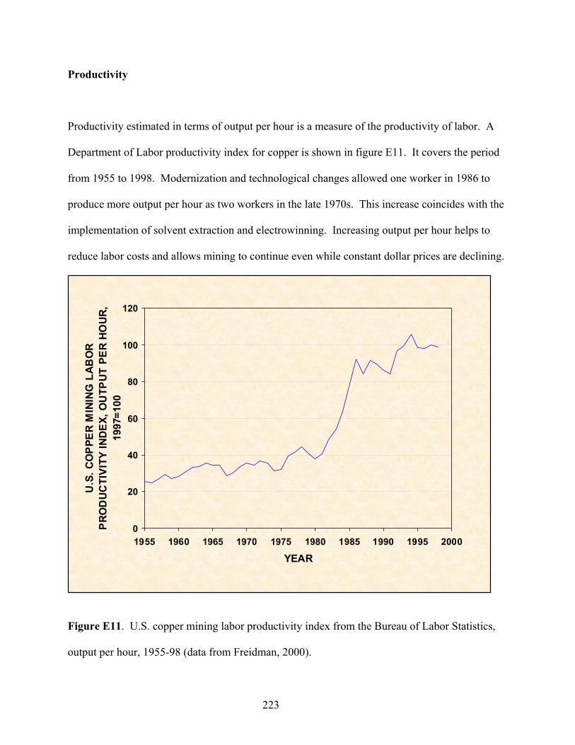
Productivity
Productivity estimated in terms of output per hour is a measure of the productivity of labor. A
Department of Labor productivity index for copper is shown in figure E11. It covers the period
from 1955 to 1998. Modernization and technological changes allowed one worker in 1986 to
produce more output per hour as two workers in the late 1970s. This increase coincides with the
implementation of solvent extraction and electrowinning. Increasing output per hour helps to
reduce labor costs and allows mining to continue even while constant dollar prices are declining.
0
20
40
60
80
100
120
1955 1960 1965 1970 1975 1980 1985 1990 1995 2000
YEAR
U.S
. CO
PPER
MIN
ING
LAB
OR
PRO
DUC
TIVI
TY IN
DEX,
OU
TPUT
PER
HO
UR,
1997
=100
Figure E11. U.S. copper mining labor productivity index from the Bureau of Labor Statistics,
output per hour, 1955-98 (data from Freidman, 2000).
223
Supply/demand relation
Copper mining operations are usually large undertakings. Copper mining entails the handling of large
quantities of material to recover the copper because the amount of copper in the ore is low; it can be less
than 1 percent (Jolly, 1985, p. 214). After the ore is removed from the ground, it is usually upgraded on
site before it is shipped to the next stage of processing. Conventional copper operations have processed
sulfide ores using flotation methods. Electrowinning technology was introduced commercially in the late
1960s and resulted in a redefinition of copper ore by including oxide ore that previously had not been
economically recoverable.
Economic theory tells us that in order to continue operating, producers have to sell their product
at a price that will allow them to recover their costs. The quantity available to the market is
affected by production costs and the market price of the commodity. When costs are so high that
a producer cannot recover them, they may cease production. This results in less material being
offered to the market. If costs are reduced and can be recovered, more material is offered to the
market. Costs affect the quantity offered to the market and therefore cause adjustments in the
supply-demand equilibrium.
Production costs are made up of operating costs, and capital costs. Operating costs include direct
operating costs such as material inputs, energy, and labor, indirect operating costs such as plant
overhead, depreciation, interest, taxes, reclamation, and general mine development. Capital
costs include exploration costs, acquisition costs, and capital equipment renewal. Table E1
contains data from the 1997 U.S. Economic Census. This Census contains a selection of total
cost data for copper mining and does not represent the total costs of a mining operation.
224
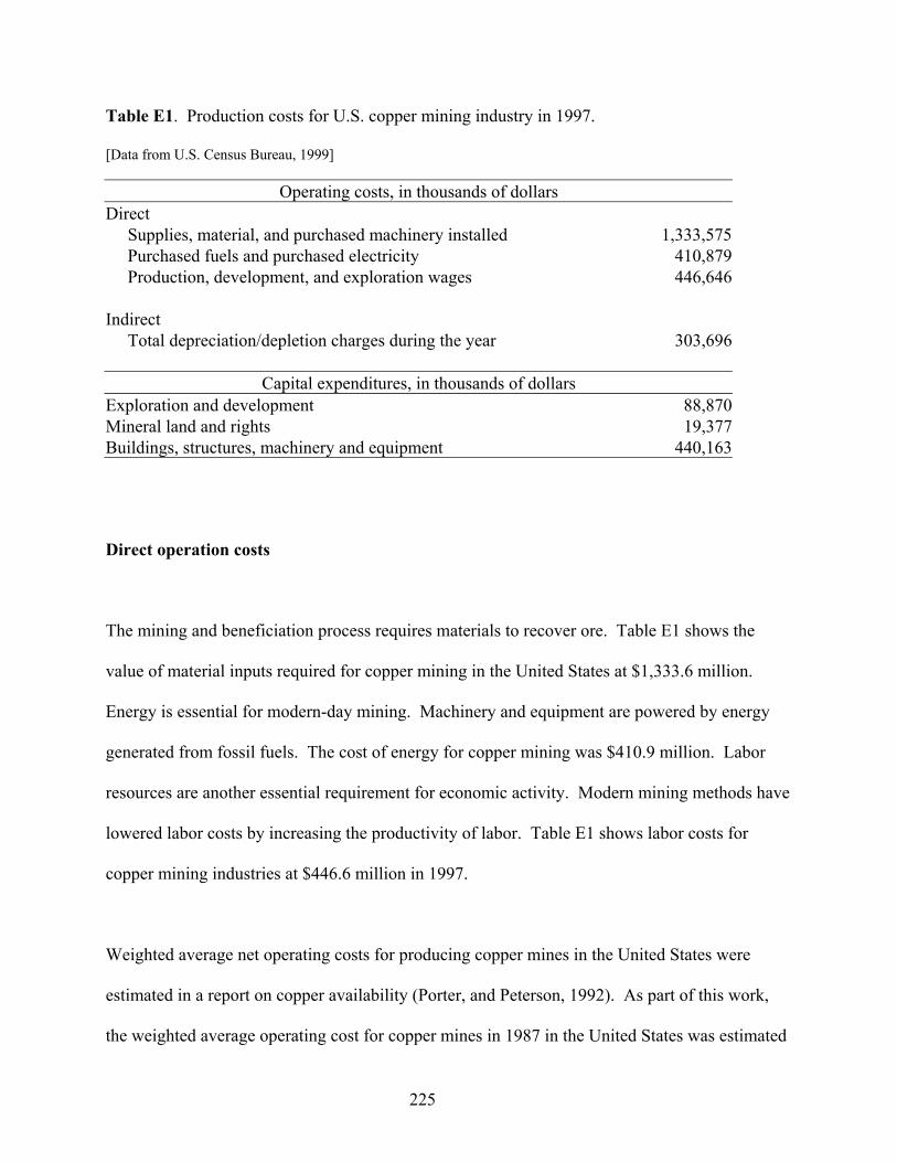
Table E1. Production costs for U.S. copper mining industry in 1997.
[Data from U.S. Census Bureau, 1999]
Operating costs, in thousands of dollars Direct Supplies, material, and purchased machinery installed 1,333,575 Purchased fuels and purchased electricity 410,879 Production, development, and exploration wages 446,646 Indirect Total depreciation/depletion charges during the year 303,696
Capital expenditures, in thousands of dollars Exploration and development 88,870Mineral land and rights 19,377Buildings, structures, machinery and equipment 440,163
Direct operation costs
The mining and beneficiation process requires materials to recover ore. Table E1 shows the
value of material inputs required for copper mining in the United States at $1,333.6 million.
Energy is essential for modern-day mining. Machinery and equipment are powered by energy
generated from fossil fuels. The cost of energy for copper mining was $410.9 million. Labor
resources are another essential requirement for economic activity. Modern mining methods have
lowered labor costs by increasing the productivity of labor. Table E1 shows labor costs for
copper mining industries at $446.6 million in 1997.
Weighted average net operating costs for producing copper mines in the United States were
estimated in a report on copper availability (Porter, and Peterson, 1992). As part of this work,
the weighted average operating cost for copper mines in 1987 in the United States was estimated
225
to be 53 cents per pound in 1987 dollars. The 1987 price of copper in 1987 dollars was 82.5
cents per pound (Porter and Edelstein, 2001).
Indirect operating costs
Indirect operating costs include items such as plant overhead that entails supervision, site
administration, facilities maintenance, research, and technical, clerical, and sales support. These
costs do not increase in direct proportion to the amount of copper produced. Depreciation is also
an indirect operating cost. Table E1 shows total copper mining depreciation charges for 1997.
Other indirect operating costs include interest, taxes, and reclamation. Reclamation is generally
a required part of mining. Modern mine planning must include reclamation and its costs, which
can be significant. The geometry of the copper deposit and how the ore is to be recovered,
among many other factors, influence the cost of reclamation. There is a wide range in the
magnitude of reclamation required around the globe, and a wide range in reclamation costs.
Administrative expenses
Administrative expenses include costs such as executive and clerical wages, office supplies,
engineering and legal expenses, upkeep on office buildings, and general communications. The
expenses connected with senior management or administrative expenses cannot be charged
directly to manufacturing costs. Therefore, it is necessary to include these costs in administrative
expenses if the economic analysis is to be complete. These costs may vary markedly from
operation to operation.
226
Sales or marketing costs and distribution costs
Few operations can be considered to be successful until the products have been sold or put to
some profitable use. It is necessary, therefore, to consider the expenses involved in selling the
products. Included in this category are salaries, wages, supplies, and other expenses for sales
offices; salaries, commissions and traveling expenses for salesmen; shipping expenses; cost of
containers; advertising expenses; and technical sales service. Sales and marketing costs vary
widely for different types of operations depending on the particular commodity produced, other
products sold by the company, plant location, and various internal and external policies.
A distribution cost is any cost incurred to market a product or service. Distribution costs may
include all amounts spent on advertising, warehousing, and shipping products to customers.
Distribution and marketing expenses are costs incurred in the process of selling and distributing
the various products. These costs include expenditures for materials handling, containers,
shipping, and other products and activities.
Research and development costs
New processes and equipment are constantly being developed as technologies evolve. The
associated research and development costs include salaries, fixed and operating expenses,
materials, supplies, and direct overhead. Usually, only larger companies have research and
development budgets for process improvements and modifications. The independent equipment
manufacturers usually do the development of equipment. The total research and development
227
costs may vary markedly from company to company. A small company may not have financial
resources required for research while larger companies with financial resources fund research. In
some cases, research and development is done by the government or a consortium.
The Phelps Dodge Corporation, a large copper producer conducts extensive research and
development. The Corporation has programs relating to technology for exploration for minerals,
recovery of metals from ores, concentrates and solutions, smelting and refining of copper, metal
processing, and product development. It also has programs related to carbon black products,
wire insulation and materials and conductor materials and processes. Expenditures for all of
these research and development programs, together with contributions to industry and
government-supported programs, totaled $24.7 million in the year 2000, compared with $16.5
million in 1999 and $18.0 million in 1998 (Phelps Dodge Corporation, 2001).
Capital costs
Some copper deposits require extensive exploration costs to be located. Acquisition costs vary
significantly as a result of many factors including the physical setting in which each deposit is
found, and the quantity and grade of ore. Properties can be acquired in order to look for deposits
or property can be purchased where the deposit that has already been discovered and defined.
Capital costs vary as a result of the capital intensity of the operation and the level of expenditures
for a given year.
228
Strategies for efficient material usage
Efficient use of copper increases the amount of copper available for use. Activities that increase
the efficiency of copper usage include substitution and recycling. Substitution takes place when
copper is either replaced by or replaces another material. This can happen when a new material
can replace copper in a specific product such as when fiber optics replaces copper in
telecommunications. A more subtle form of material substitution occurs when a new product
using different materials replaces the function of an original product, such as nonmetallic
microwavable bowl replaces a copper saucepan. Substitution utilizes more economically
available materials, thus contributing to efficient material usage. It also reduces the likelihood of
materials scarcity.
Recycling is when copper is recovered at the end of the copper containing product’s useful life.
The value of copper is usually sufficient to make recovering it profitable. When natural market
forces or are not sufficient to stimulate copper recycling, regulations or taxes make recycling
financially attractive. When copper is recycled, it becomes a valuable resource instead of waste.
By supplementing the quantity of copper available to the market, recycling conserves virgin
copper and makes more copper available to the market. Copper used in construction is an
example of material that once it is put in place can continue to be used for 30 to 50 years and
longer. Copper lends itself to recycling. The apparent supply of copper from recycled sources
was nearly 33 percent in 1999, but has been declining in recent years. The rate was almost 39
percent in 1995 (U.S. Geological Survey, 2001, p. 62.15). Recycling of copper is sensitive to
229
price as scrap copper prices tend to follow refined copper prices. When prices are low, the scrap
processors find it more difficult to compete with primary copper.
Source reduction means utilizing less of copper to attain the same economic benefit. This can be
done with a change in design, more efficient manufacturing methods, or more efficient usage of
products. As an example, when electronic products are minimized, less copper is required to
perform the same function. Source reduction saves natural resources, reduces waste, and reduces
costs.
Conclusions
Apparent consumption of copper has increased over the 20th century, supported by increased
domestic production and net imports. Early in the 20th century, the U.S. economy’s need for
copper was satisfied using domestic ores. Through the century, as requirements increased, new
deposits were found and new technologies were developed. With globalization, ores were
imported to help satisfy the economy’s need for copper. As a result of this increased availability
of copper, the constant dollar price of copper has been declining. The domestic industry has
been able to remain competitive by increases in productivity and through technological
innovations.
230
References
Butterman, W.C., 1982, Copper, in Mineral Commodity Summaries, 1982: U.S. Bureau of Mines, p. 40-41. Edelstein, D.L., 2001, Copper, in Mineral Commodity Summaries, 2001: U.S. Geological Survey, p. 52-53. Jolly, J.L.W., 1985, Copper, in Mineral Facts and Problems, 1985 edition: U.S. Bureau of Mines Bulletin 675, p. 197-221. Phelps Dodge Corporation, 2001, Form 10-K– For the fiscal year ended December 31, 2000: Phelps Dodge Corporation, 92 p. Porter, K.E., and Edelstein, D.L., 2001, Copper statistics, in Historical statistics for mineral commodities in the United States: U.S. Geological Survey Open-File Report 01-006. Porter, K.E., and Peterson, G.R., 1992, The availability of primary copper in market economy countries– A minerals availability appraisal: U.S. Bureau of Mines Information Circular 9310, 32 p. U.S. Census Bureau, 1999, Copper ore and nickel ore mining, in 1997 Economic Census- Mining: U.S. Census Bureau, EC97N-2122EB, 10 p. U.S. Geological Survey, 2001, Recycling–Metals, in Metals and Minerals: U.S. Geological Survey Minerals Yearbook 1999, v. I, p. 62.1-62.17. Wilburn, D.A., Goonan, T.G., and Bleiwas, D.A., 2001, Technological advancement– A factor in increasing resource use: U.S. Geological Survey Open-File Report 01-197.
Internet references cited U.S. Census Bureau, 2000, Historical national population estimates– July 1, 1900 to July 1, 1999, accessed May 6, 2002, at URL http://eire.census.gov/popest/archives/pre1980/popclockest.txt. U.S. Census Bureau, 2001, Table US-2001EST-01 – Time series national population estimates – April 1, 2000 to July 1, 2001, accessed May 6, 2002, at URL http://eire.census.gov/popest/data/national/populartables/table01.php].
231
APPENDIX F: ECONOMIC CASE STUDY -- POTASH
Introduction/background
During colonial times, potash was produced by burning wood, leaching the soluble salts from the
ashes, and recrystallizing them in iron pots. At this time, potash was used to make soap and
glass. Significant world production began in Europe in the middle of the 19th century. Germany
was an important source of potash; however this source was cut off during World War I. The
U.S. potash mining industry began developing in response to the resulting shortages. The
development of mines near Carlsbad, New Mexico in the 1930s made the United States nearly
independent of imported potash. This lasted until 1962 when increasing production from large
Canadian sources began to affect the U.S. market (Searls, 1985).
About 90 percent of U.S. potash sales are used by the fertilizer industry (Searls, 2001). Potash
contains potassium, which is one of the three main ingredients in fertilizer along with nitrogen
and phosphorus. Potash is usually defined as any form of water-soluble potassium salt that can
be produced, transported to the crop acreage, and spread over the acreage to the economic
benefit of the farmer. The most common form of potash is potassium chloride. Additional forms
of potash are potassium magnesium sulfate, potassium nitrate, and potassium-sodium nitrate.
Potassium oxide, which is not usually considered potash, is used in ceramics. In order to
evaluate the amount of potassium in the various types of potash the grade is calculated in terms
of K2O (Searls, 1985, p. 617-619).
232
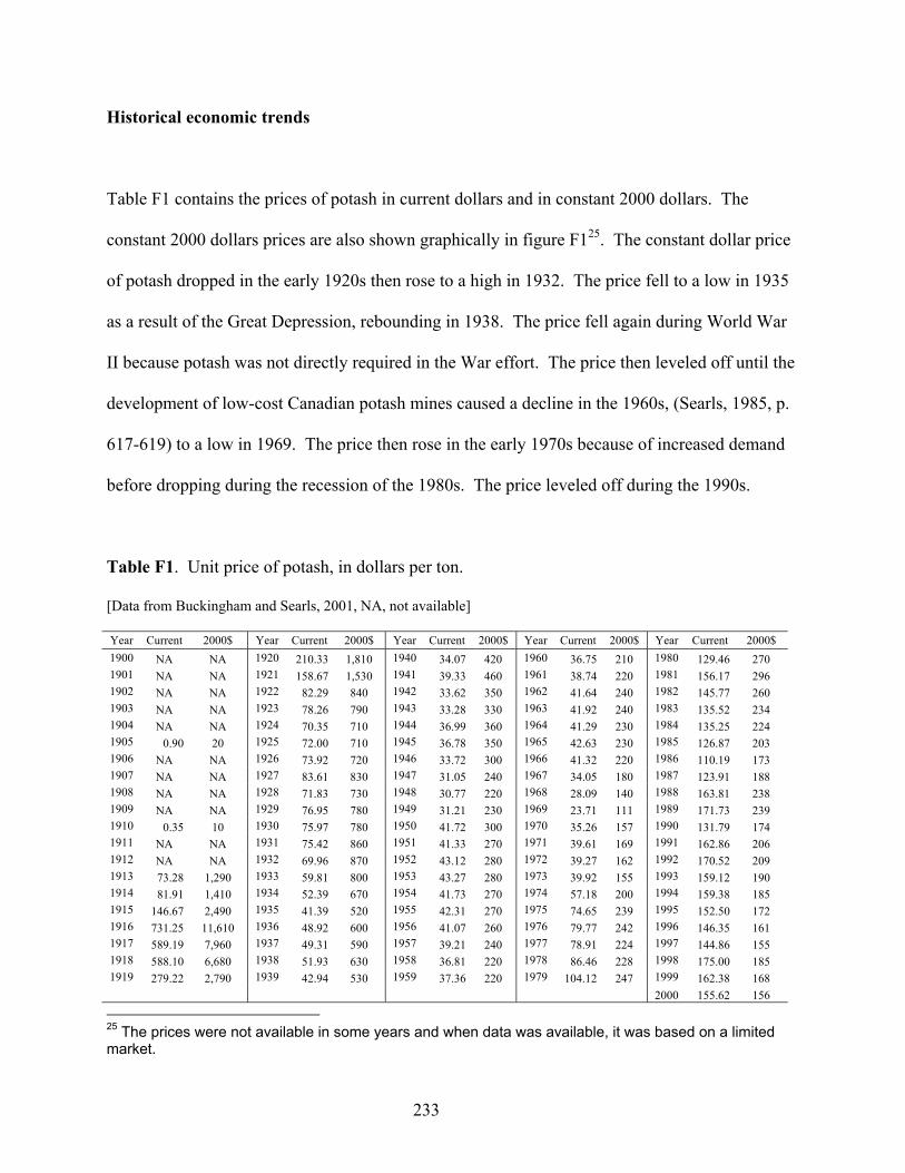
Historical economic trends
Table F1. Unit price of potash, in dollars per ton.
Table F1 contains the prices of potash in current dollars and in constant 2000 dollars. The
constant 2000 dollars prices are also shown graphically in figure F125. The constant dollar price
of potash dropped in the early 1920s then rose to a high in 1932. The price fell to a low in 1935
as a result of the Great Depression, rebounding in 1938. The price fell again during World War
II because potash was not directly required in the War effort. The price then leveled off until the
development of low-cost Canadian potash mines caused a decline in the 1960s, (Searls, 1985, p.
617-619) to a low in 1969. The price then rose in the early 1970s because of increased demand
before dropping during the recession of the 1980s. The price leveled off during the 1990s.
[Data from Buckingham and Searls, 2001, NA, not available]
Year Current 2000$ Year Current 2000$ Year Current 2000$ Year Current 2000$ Year Current 2000$ 1900 NA NA 1920 210.33 1,810 1940 34.07 420 1960 36.75 210 1980 129.46 270 1901 NA NA 1921 158.67 1,530 1941 39.33 460 1961 38.74 220 1981 156.17 296 1902 NA NA 1922 82.29 840 1942 33.62 350 1962 41.64 240 145.771982 260 1903 NA 78.26 790 330 NA 1923 1943 33.28 1963 41.92 240 1983 135.52 234 1904 NA NA 1924 70.35 710 1944 36.99 360 1964 41.29 230 1984 135.25 224 1905 0.90 20 1925 72.00 710 1945 36.78 350 1965 42.63 230 1985 126.87 203 1906 NA NA 1926 73.92 720 1946 33.72 300 1966 41.32 220 1986 110.19 173 1907 NA NA 1927 83.61 830 1947 31.05 240 1967 34.05 180 1987 123.91 188 1908 NA NA 1928 71.83 730 1948 30.77 220 1968 28.09 140 1988 163.81 238 1909 NA NA 1929 76.95 780 1949 31.21 230 1969 23.71 111 1989 171.73 239 1910 0.35 10 1930 75.97 780 1950 41.72 300 1970 35.26 157 1990 131.79 174 1911 NA NA 1931 75.42 860 1951 41.33 270 1971 39.61 169 1991 162.86 206
NA NA 1932 69.96 870 1952 43.12 280 1972 39.27 162 1992 170.52 209 1913 73.28 1,290 1933 59.81 800 1953 43.27 280 1973 39.92 155 1993 159.12 190 1914 81.91 1,410 1934 52.39 670 1954 41.73 270 1974 57.18 200 1994 159.38 185 1915 146.67 2,490 1935 41.39 520 1955 42.31 270 1975 74.65 239 1995 152.50 172 1916 731.25 11,610 1936 48.92 600 1956 41.07 260 1976 79.77 242 1996 146.35 161 1917 589.19 7,960 1937 49.31 590 1957 39.21 240 1977 78.91 224 1997 144.86 155 1918 588.10 6,680 1938 51.93 630 1958 36.81 220 1978 86.46 228 1998 175.00 185 1919 279.22 2,790 1939 42.94 530 1959 37.36 220 1979 104.12 247 1999 162.38 168
2000 155.62 156
1912
25 The prices were not available in some years and when data was available, it was based on a limited market.
233
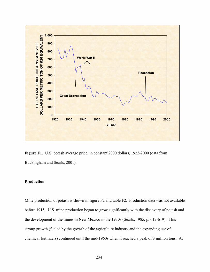
0
100
200
300
400
500
600
700
800
900
1,000
1920 1930 1940 1950 1960 1970 1980 1990 2000
YEAR
U.S.
PO
TASH
PRI
CE, I
N C
ONS
TANT
200
0 D
OLL
AR
S PE
R M
ETR
IC T
ON
OF
K20
EQ
UIVA
LENT
World War II
Recession
Great Depression
Figure F1. U.S. potash average price, in constant 2000 dollars, 1922-2000 (data from
Buckingham and Searls, 2001).
Production
Mine production of potash is shown in figure F2 and table F2. Production data was not available
before 1915. U.S. mine production began to grow significantly with the discovery of potash and
the development of the mines in New Mexico in the 1930s (Searls, 1985, p. 617-619). This
strong growth (fueled by the growth of the agriculture industry and the expanding use of
chemical fertilizers) continued until the mid-1960s when it reached a peak of 3 million tons. At
234
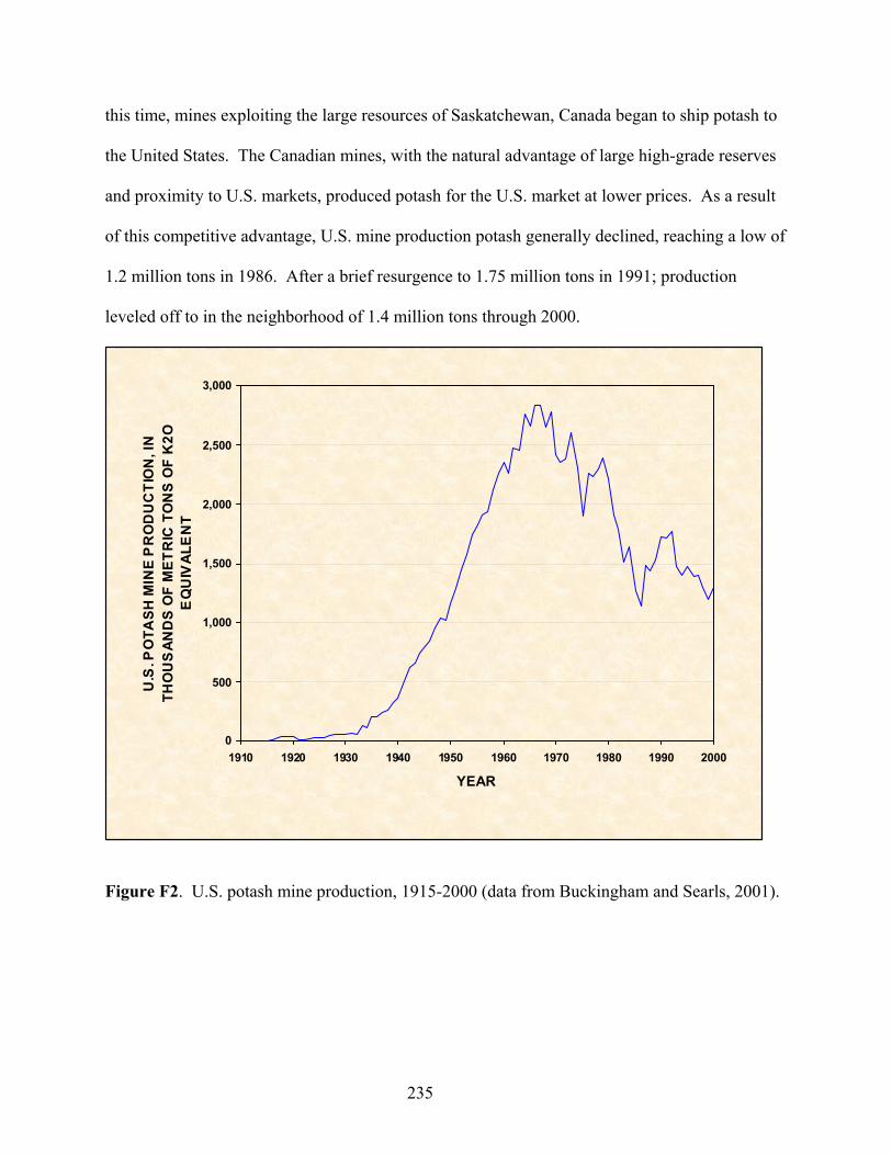
this time, mines exploiting the large resources of Saskatchewan, Canada began to ship potash to
the United States. The Canadian mines, with the natural advantage of large high-grade reserves
and proximity to U.S. markets, produced potash for the U.S. market at lower prices. As a result
of this competitive advantage, U.S. mine production potash generally declined, reaching a low of
1.2 million tons in 1986. After a brief resurgence to 1.75 million tons in 1991; production
leveled off to in the neighborhood of 1.4 million tons through 2000.
0
500
1,000
1,500
2,000
2,500
3,000
1910 1920 1930 1940 1950 1960 1970 1980 1990 2000
YEAR
U.S
. PO
TASH
MIN
E P
RO
DU
CTI
ON
, IN
TH
OU
SAN
DS
OF
MET
RIC
TO
NS
OF
K2O
E
QU
IVAL
EN
T
Figure F2. U.S. potash mine production, 1915-2000 (data from Buckingham and Searls, 2001).
235
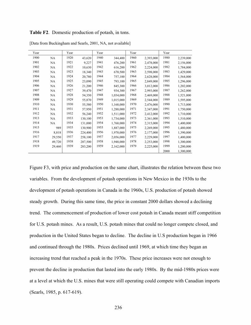
Table F2. Domestic production of potash, in tons.
[Data from Buckingham and Searls, 2001, NA, not available]
Year Year Year Year Year 1900 NA 1920 43,620 1940 344,400 1960 2,393,000 1980 2,239,000 1901 NA 1921 9,227 1941 476,200 1961 2,478,000 1981 2,156,000 1902 NA 1922 10,630 1942 616,200 1962 2,224,000 1982 1,784,000 1903 NA 1923 18,340 1943 670,500 1963 2,598,000 1983 1,429,000 1904 NA 1924 20,780 1944 757,100 1964 2,628,000 1984 1,564,000 1905 NA 1925 23,090 1945 793,100 1965 2,849,000 1985 1,296,000 1906 NA 1926 21,200 1946 845,300 1966 3,012,000 1986 1,202,000 1907 NA 1927 39,470 1947 934,300 1967 2,993,000 1987 1,262,000 1908 NA 1928 54,350 1948 1,034,000 1968 2,469,000 1988 1,521,000 1909 NA 1929 55,870 1949 1,015,000 1969 2,544,000 1989 1,595,000 1910 NA 1930 55,580 1950 1,168,000 1970 2,476,000 1990 1,713,000 1911 NA 1931 57,950 1951 1,288,000 1971 2,347,000 1991 1,750,000 1912 NA 1932 56,240 1952 1,511,000 1972 2,412,000 1992 1,710,000 1913 NA 1933 130,100 1953 1,734,000 1973 2,361,000 1993 1,510,000 1914 NA 1934 131,000 1954 1,768,000 1974 2,315,000 1994 1,400,000 1915 989 1935 130,900 1955 1,887,000 1975 2,269,000 1995 1,480,000 1916 8,818 1936 224,400 1956 1,970,000 1976 2,177,000 1996 1,390,000 1917 29,550 1937 258,100 1957 2,056,000 1977 2,229,000 1997 1,400,000 1918 49,720 1938 287,500 1958 1,948,000 1978 2,253,000 1998 1,300,000 1919 29,460 1939 283,200 1959 2,162,000 1979 2,225,000 1999 1,200,000
2000 1,300,000
Figure F3, with price and production on the same chart, illustrates the relation between these two
variables. From the development of potash operations in New Mexico in the 1930s to the
development of potash operations in Canada in the 1960s, U.S. production of potash showed
steady growth. During this same time, the price in constant 2000 dollars showed a declining
trend. The commencement of production of lower cost potash in Canada meant stiff competition
for U.S. potash mines. As a result, U.S. potash mines that could no longer compete closed, and
production in the United States began to decline. The decline in U.S production began in 1966
and continued through the 1980s. Prices declined until 1969, at which time they began an
increasing trend that reached a peak in the 1970s. These price increases were not enough to
prevent the decline in production that lasted into the early 1980s. By the mid-1980s prices were
at a level at which the U.S. mines that were still operating could compete with Canadian imports
(Searls, 1985, p. 617-619).
236
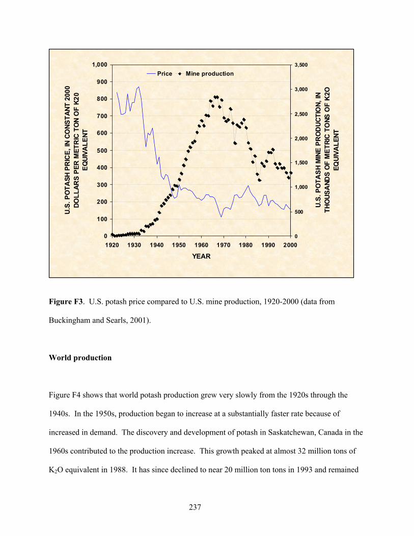
0
100
200
300
400
500
600
700
800
900
1,000
1920 1930 1940 1950 1960 1970 1980 1990 2000
YEAR
U.S.
PO
TASH
PR
ICE,
IN C
ONS
TANT
200
0 DO
LLAR
S PE
R M
ETR
IC T
ON
OF
K20
EQUI
VALE
NT
0
500
1,000
1,500
2,000
2,500
3,000
3,500
U.S.
PO
TASH
MIN
E PR
OD
UCTI
ON,
IN
THO
USA
NDS
OF
MET
RIC
TO
NS O
F K
2O
EQUI
VALE
NT
Price Mine production
Figure F3. U.S. potash price compared to U.S. mine production, 1920-2000 (data from
Buckingham and Searls, 2001).
World production
Figure F4 shows that world potash production grew very slowly from the 1920s through the
1940s. In the 1950s, production began to increase at a substantially faster rate because of
increased in demand. The discovery and development of potash in Saskatchewan, Canada in the
1960s contributed to the production increase. This growth peaked at almost 32 million tons of
K2O equivalent in 1988. It has since declined to near 20 million ton tons in 1993 and remained
237
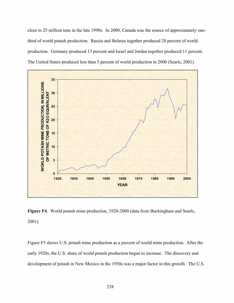
close to 25 million tons in the late 1990s. In 2000, Canada was the source of approximately one-
third of world potash production. Russia and Belarus together produced 28 percent of world
production. Germany produced 13 percent and Israel and Jordan together produced 11 percent.
The United States produced less than 5 percent of world production in 2000 (Searls, 2001).
0
5
10
15
20
25
30
35
1920 1930 1940 1950 1960 1970 1980 1990 2000
YEAR
WO
RLD
PO
TASH
MIN
E PR
ODU
CTI
ON,
IN M
ILLI
ONS
O
F M
ETR
IC T
ONS
OF
K2O
EQ
UIVA
LENT
Figure F4. World potash mine production, 1920-2000 (data from Buckingham and Searls,
2001).
Figure F5 shows U.S. potash mine production as a percent of world mine production. After the
early 1920s, the U.S. share of world potash production began to increase. The discovery and
development of potash in New Mexico in the 1930s was a major factor in this growth. The U.S.
238
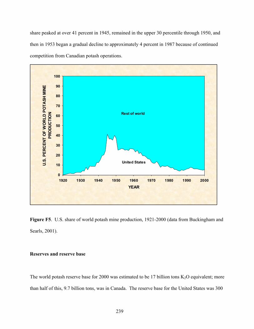
share peaked at over 41 percent in 1945, remained in the upper 30 percentile through 1950, and
then in 1953 began a gradual decline to approximately 4 percent in 1987 because of continued
competition from Canadian potash operations.
United States
0
10
20
30
40
50
60
70
80
90
100
1920 1930 1940 1950 1960 1970 1980 1990 2000
YEAR
U.S.
PER
CEN
T O
F W
OR
LD P
OTA
SH M
INE
PRO
DUC
TIO
N Rest of world
Figure F5. U.S. share of world potash mine production, 1921-2000 (data from Buckingham and
Searls, 2001).
Reserves and reserve base
The world potash reserve base for 2000 was estimated to be 17 billion tons K2O equivalent; more
than half of this, 9.7 billion tons, was in Canada. The reserve base for the United States was 300
239

million tons, less than 2 percent of the world estimate. World reserves were estimated to be 8.4
billion tons K2O equivalent; more than half of this, 4.4 billion tons, was in Canada. Those of the
United States were 100 million tons, about 1 percent of the world total (Searls, 2001).
Use
Potash use in the United States as measured by apparent consumption (figure F6) had a strong
increasing trend until 1979 when it reached a peak of 6.9 million tons K2O equivalent. Apparent
consumption is defined as production plus imports minus exports plus or minus changes in
stocks. This increase in fertilizer usage was fueled by a strong increase in the production of
grain crops. After the peak in 1979, apparent consumption dropped to a low of 4.5 million tons
in 1989. The high relative value of the dollar in 1980 and 1981 on the international market led to
poor sales of U.S. grains. This caused reductions in prices, thus lowering profits for U.S. farmers
in 1982 and 1983. Lower profits in turn reduced the capability of growers to purchase potash
fertilizers, (Searls, 1985). Since that time, the demand for fertilizer increased, and potash usage
has trended upward, to above 6 million in the late 1990s.
240
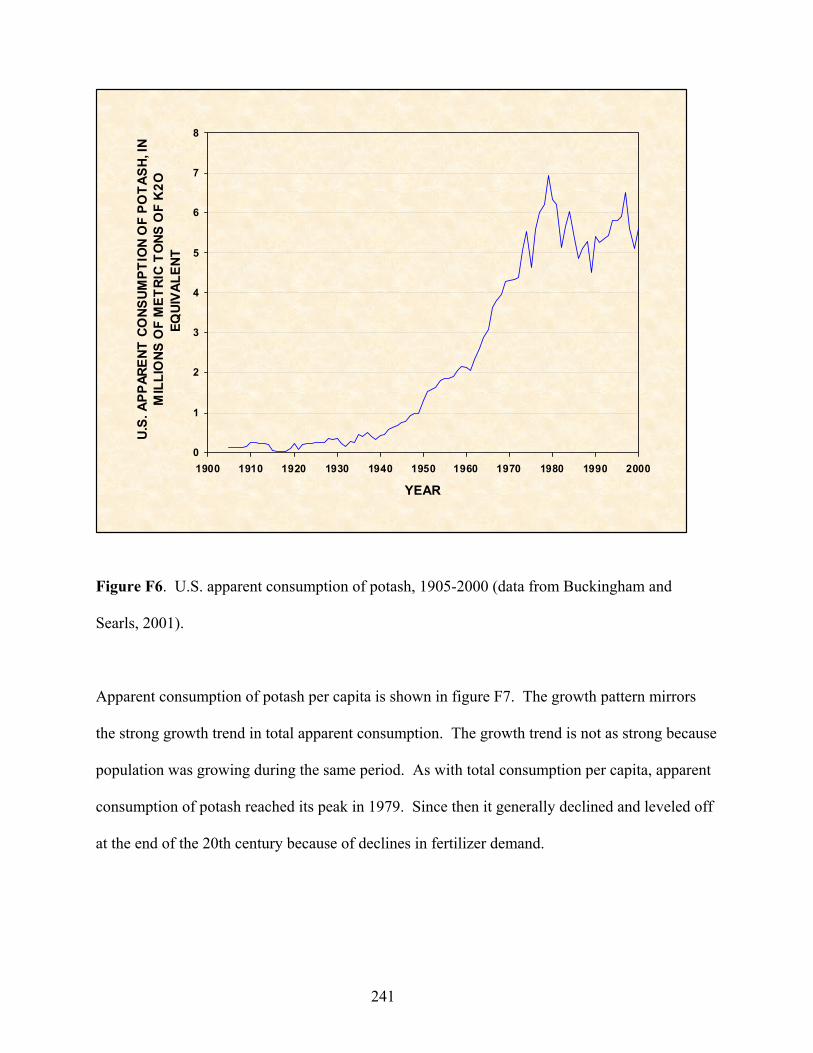
0
1
2
3
4
5
6
7
8
1900 1910 1920 1930 1940 1950 1960 1970 1980 1990 2000
YEAR
U.S.
APP
AREN
T CO
NSUM
PTIO
N O
F PO
TASH
, IN
MIL
LIO
NS O
F M
ETRI
C TO
NS O
F K
2O
EQUI
VALE
NT
Figure F6. U.S. apparent consumption of potash, 1905-2000 (data from Buckingham and
Searls, 2001).
Apparent consumption of potash per capita is shown in figure F7. The growth pattern mirrors
the strong growth trend in total apparent consumption. The growth trend is not as strong because
population was growing during the same period. As with total consumption per capita, apparent
consumption of potash reached its peak in 1979. Since then it generally declined and leveled off
at the end of the 20th century because of declines in fertilizer demand.
241
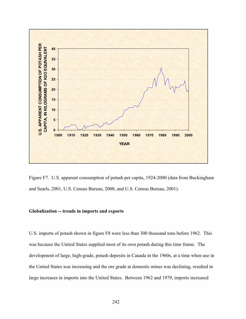
0
5
10
15
20
25
30
35
40
1900 1910 1920 1930 1940 1950 1960 1970 1980 1990 2000
YEAR
U.S.
APP
ARE
NT C
ONS
UMPT
ION
OF
POTA
SH P
ER
CAPI
TA, I
N KI
LOG
RAM
S O
F K2
O E
QUI
VALE
NT
Figure F7. U.S. apparent consumption of potash per capita, 1924-2000 (data from Buckingham
and Searls, 2001, U.S. Census Bureau, 2000, and U.S. Census Bureau, 2001).
Globalization -- trends in imports and exports
U.S. imports of potash shown in figure F8 were less than 300 thousand tons before 1962. This
was because the United States supplied most of its own potash during this time frame. The
development of large, high-grade, potash deposits in Canada in the 1960s, at a time when use in
the United States was increasing and the ore grade at domestic mines was declining, resulted in
large increases in imports into the United States. Between 1962 and 1979, imports increased
242
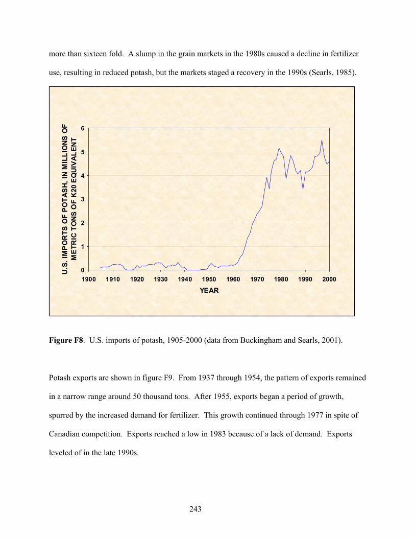
more than sixteen fold. A slump in the grain markets in the 1980s caused a decline in fertilizer
use, resulting in reduced potash, but the markets staged a recovery in the 1990s (Searls, 1985).
0
1
2
3
4
5
6
1900 1910 1920 1930 1940 1950 1960 1970 1980 1990 2000
YEAR
U.S
. IM
POR
TS O
F PO
TASH
, IN
MIL
LIO
NS O
F M
ETR
IC T
ONS
OF
K20
EQ
UIVA
LEN
T
Figure F8. U.S. imports of potash, 1905-2000 (data from Buckingham and Searls, 2001).
Potash exports are shown in figure F9. From 1937 through 1954, the pattern of exports remained
in a narrow range around 50 thousand tons. After 1955, exports began a period of growth,
spurred by the increased demand for fertilizer. This growth continued through 1977 in spite of
Canadian competition. Exports reached a low in 1983 because of a lack of demand. Exports
leveled of in the late 1990s.
243
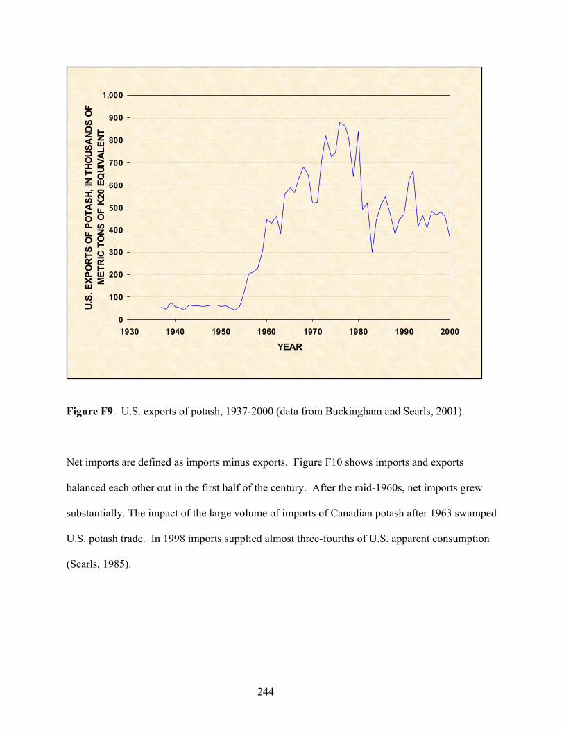
0
100
200
300
400
500
600
700
800
900
1,000
1930 1940 1950 1960 1970 1980 1990 2000
YEAR
U.S.
EXP
OR
TS O
F PO
TASH
, IN
THO
USA
NDS
OF
MET
RIC
TO
NS O
F K
20 E
QUI
VALE
NT
Figure F9. U.S. exports of potash, 1937-2000 (data from Buckingham and Searls, 2001).
Net imports are defined as imports minus exports. Figure F10 shows imports and exports
balanced each other out in the first half of the century. After the mid-1960s, net imports grew
substantially. The impact of the large volume of imports of Canadian potash after 1963 swamped
U.S. potash trade. In 1998 imports supplied almost three-fourths of U.S. apparent consumption
(Searls, 1985).
244
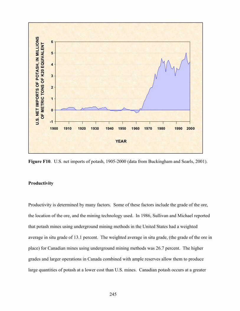
-1
0
1
2
3
4
5
6
YEAR
U.S.
NET
IMPO
RTS
OF
POTA
SH, I
N M
ILLI
ONS
O
F M
ETR
IC T
ONS
OF
K20
EQ
UIVA
LEN
T
1900 1910 1920 1940 1950 1960 1970 1980 1990 20001930
Figure F10. U.S. net imports of potash, 1905-2000 (data from Buckingham and Searls, 2001).
Productivity
Productivity is determined by many factors. Some of these factors include the grade of the ore,
the location of the ore, and the mining technology used. In 1986, Sullivan and Michael reported
that potash mines using underground mining methods in the United States had a weighted
average in situ grade of 13.1 percent. The weighted average in situ grade, (the grade of the ore in
place) for Canadian mines using underground mining methods was 26.7 percent. The higher
grades and larger operations in Canada combined with ample reserves allow them to produce
large quantities of potash at a lower cost than U.S. mines. Canadian potash occurs at a greater
245
depth requiring that a larger quantity of potash be left in the form of pillars (Sullivan and
Michael, 1986). This affects the percent of in situ ore recovered but does not prevent the
Canadian mines from operating at lower costs because of the substantially higher grade.
Costs
Potash mining operations use underground mining methods (room and pillar, sublevel stoping,
longwall caving, and cut-and-fill stoping), solution mining, and brine recovery. Potash is mined,
sold, and used in large volumes so mining entails the handling of large quantities of material.
After the potash ore is mined, it is upgraded (beneficiated) on site before it is shipped.
Beneficiation methods include washing, flotation, and crystallization (Sullivan and Michael,
1986).
The quantity producers are willing to sell is a result of their production costs and the market
price of the commodity. Production costs are made up of operating costs and capital costs.
Operating costs include direct operating costs such as material inputs, energy, and labor, indirect
operating costs such as plant overhead, depreciation, interest, taxes, reclamation, and general
mine development. Capital costs include exploration costs, acquisition costs, and capital
equipment renewal.
246
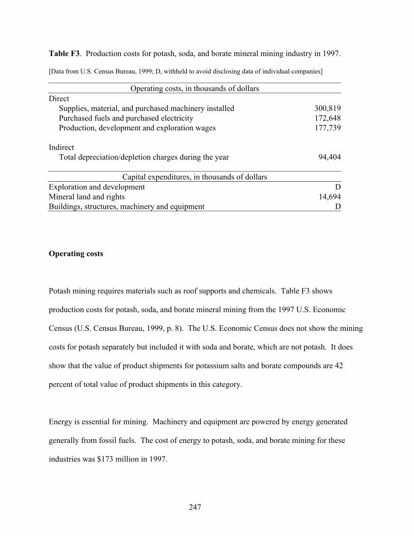
Table F3. Production costs for potash, soda, and borate mineral mining industry in 1997.
[Data from U.S. Census Bureau, 1999; D, withheld to avoid disclosing data of individual companies]
Operating costs, in thousands of dollars Direct Supplies, material, and purchased machinery installed 300,819 Purchased fuels and purchased electricity 172,648 Production, development and exploration wages 177,739 Indirect Total depreciation/depletion charges during the year 94,404
Capital expenditures, in thousands of dollars Exploration and development DMineral land and rights 14,694Buildings, structures, machinery and equipment D
Operating costs
Potash mining requires materials such as roof supports and chemicals. Table F3 shows
production costs for potash, soda, and borate mineral mining from the 1997 U.S. Economic
Census (U.S. Census Bureau, 1999, p. 8). The U.S. Economic Census does not show the mining
costs for potash separately but included it with soda and borate, which are not potash. It does
show that the value of product shipments for potassium salts and borate compounds are 42
percent of total value of product shipments in this category.
Energy is essential for mining. Machinery and equipment are powered by energy generated
generally from fossil fuels. The cost of energy to potash, soda, and borate mining for these
industries was $173 million in 1997.
247
Labor resources are another essential requirement for economic activity. Modern mining
methods have lowered labor costs by increasing the productivity of labor. The table shows labor
costs at $178 million for potash, soda, and borate mining in 1997.
Indirect operating costs include items such as plant overhead that entails supervision, site
administration, facilities maintenance, research, and technical, clerical, and sales force. These
costs do not increase in direct proportion to the amount of material produced. Depreciation is an
indirect operating cost. The table shows total depreciation charges during the year for 1997.
Depreciation was $94 million for the potash, soda, and borate mining industry.
In 1987, the U.S. Bureau of Mines published estimates for net operating costs for underground
muriate of potash producers in the United States, Canada and Europe (U.S. Bureau of Mines,
1987). Net operating costs includes transportation and credits for byproducts. Net operating
costs for mines in the United States were $96.50 per ton in January 1985 dollars. Canadian
mines net operating costs were $55.60 and net operating costs for mines in Europe were $14.90
(note: the mines evaluated in Europe had large credits for byproducts and low transportation
costs).
Strategies for efficient material usage
Potassium, along with nitrogen and phosphorus, is an essential nutrient for plant growth and is
used extensively in fertilizers. Fertilizers complement naturally occurring potassium in the soil
and may be considered a substitute for soil potash when it is lacking. The most efficient
248
application of fertilizers can result in the highest crop yields. When potash is used as a fertilizer,
it is dissipated into the environment and is not available for recycling.
Source reduction means utilizing less material to attain the same economic benefit. This has the
effect of reducing the requirement for materials. Source reduction could occur in fertilizers if
they are applied carefully so as not to be used excessively. Global Positioning Systems (GPS)
using satellites are used to insure the correct application of fertilizers. Soil samples are taken in a
grid pattern and the GPS is used to determine what area of the grid is being treated to apply the
appropriate amount of fertilizer (Russell E. Koeller Family Farms, 2001§). Source reduction
saves natural resources, reduces waste, and reduces costs.
Conclusions
The United States was self-sufficient in potash from the 1930s until the development of
Canadian potash operations in the 1960s. Since that time, the bulk of potash used in the United
States has come from Canada. Because Canada has large reserves of potash, scarcity is not an
issue, and there is little concern of running out of potash. The price of potash in 2000 dollars has
a downward overall trend from 1922 through 2000. Prices in the late 1990s were less than those
in the late 1950s. They reached a low below $110 in 1969 and a high above $294 in 1981.
These price fluctuations were products of political and economic factors other than scarcity.
249
References
Buckingham, D.A., and Searls, J.P., 2001, Potash statistics, in Historical statistics for mineral commodities in the United States: U.S. Geological Survey Open-File Report 01-006. Searls, J.P., 1985, Potash, in Mineral Facts and Problems, 1985 edition: U.S. Bureau of Mines Bulletin 675, p. 617-633. Searls, J.P., 2001, Potash, in Mineral Commodity Summaries, 2001: U.S. Geological Survey, p. 124-125. Sullivan, D.E., and Michael, Nicholas, 1986, Potash availability – Market economy countries: U.S. Bureau of Mines Information Circular 9084, 32 p. U.S. Bureau of Mines, 1987, Potash, in An Appraisal of Minerals Availability for 34 Commodities: U.S. Bureau of Mines, Bulletin 692, 1987, p. 229-237. U.S. Census Bureau, 1999, Potash, soda, and borate mineral mining, in 1997 Economic Census- Mining: U.S. Census Bureau, EC97N-2123I, 10 p. Internet references cited Russell E. Koeller Family Farms, 2001, Field photo, accessed November 9, 2001, at URL http://www.koeller.com/fieldphoto.html. U.S. Census Bureau, 2000, Historical national population estimates– July 1, 1900 to July 1, 1999, accessed May 6, 2002, at URL http://eire.census.gov/popest/archives/pre1980/popclockest.txt. U.S. Census Bureau, 2001, Table US-2001EST-01 – Time series national population estimates – April 1, 2000 to July 1, 2001, accessed May 6, 2002, at URL http://eire.census.gov/popest/data/national/populartables/table01.php.
250
APPENDIX G. ECONOMIC CASE STUDY – SULFUR
Introduction/background
Sulfur (chemical symbol S), is a tasteless, odorless, nonmetallic element. Also called brimstone
(liquid sulfur) because it was synonymous with fire and evil, sulfur has been known since
prehistoric times (Microsoft® Encarta® Online Encyclopedia, 2002§). Sulfur is the raw material
for sulfuric acid processing and the manufacturing of other materials. Its consumption has been
regarded as an index of a nation’s industrial development (Buckingham, 1986).
Sulfur occurs freely in the vicinity of volcanoes and hot springs and is often associated with
limestone, gypsum, natural gas, and petroleum. Sulfur deposits are found in Iceland, Italy,
Japan, Mexico, and Spain. The island of Sicily (Italy) was the major supplier for the world until
the beginning of the 20th century.
Sulfur and sulfuric acid are largely consumed in the manufacture of various products such as
fertilizers, gunpowder, insecticides, and sulfa drugs. Chemically, sulfur combines with hydrogen
to form hydrogen sulfide (H2S), a colorless, poisonous gas with the smell of rotten eggs. When
burned in air, sulfur combines with oxygen to form sulfur dioxide (SO2). In moist air, SO2
oxidizes to sulfuric acid (H2SO4), sulfur’s most important compound (Morse, 1985). Figure G1
presents sulfur and sulfuric acid flows from origination through various applications and shows
industry classifications.
251
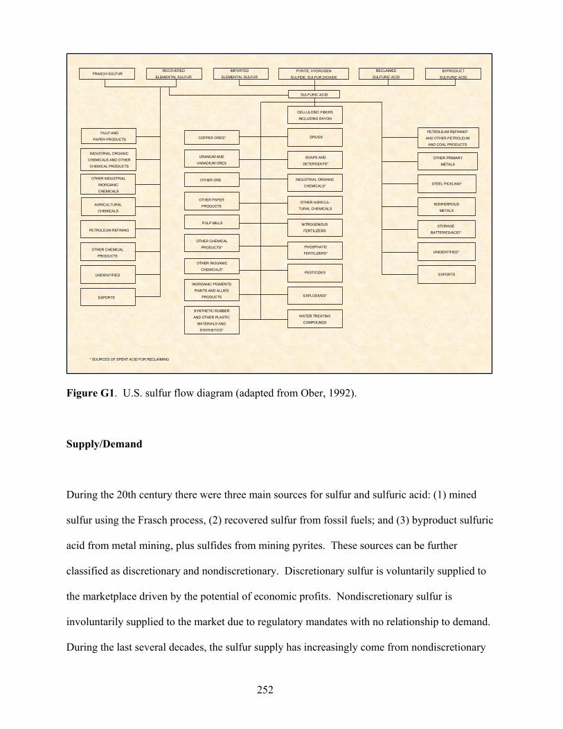
SULFURIC ACID
FRASCH SULFURRECOVERED
ELEMENTAL SULFUR
BYPRODUCT
SULFURIC ACID
IMPORTED
ELEMENTAL SULFUR
RECLAIMED
SULFURIC ACID
DRUGS
CELLULOSIC FIBERS
INCLUDING RAYON
PYRITE, HYDROGEN
SULFIDE, SULFUR DIOXIDE
PULP AND
PAPER PRODUCTS
INDUSTRIAL ORGANIC
CHEMICALS AND OTHER
CHEMICAL PRODUCTS
COPPER ORES*
SOAPS AND
DETERGENTS*
URANIUM AND
VANADIUM ORESOTHER PRIMARY
METALS
STEEL PICKLING*
PETROLEUM REFINING*
AND OTHER PETROLEUM
AND COAL PRODUCTS
INDUSTRIAL ORGANIC
CHEMICALS*OTHER OREOTHER INDUSTRIAL
INORGANIC
CHEMICALS
NONFERROUS
METALS
OTHER PAPER
PRODUCTSOTHER AGRICUL-
TURAL CHEMICALSAGRICULTURAL
CHEMICALS
PULP MILLS
OTHER CHEMICAL
PRODUCTS
PETROLEUM REFINING
UNIDENTIFIED* PHOSPHATIC
FERTILIZERS*
STORAGE
BATTERIES/ACID*
WATER TREATING
COMPOUNDS
INORGANIC PIGMENTS
PAINTS AND ALLIED
PRODUCTS
OTHER INOGANIC
CHEMICALS*
EXPORTS
UNIDENTIFIED EXPORTS
EXPLOSIVES*
SYNTHETIC RUBBER
AND OTHER PLASTIC
MATERIALS AND
SYNTHETICS*
PESTICIDES
NITROGENOUS
FERTILIZERS
OTHER CHEMICAL
PRODUCTS*
* SOURCES OF SPENT ACID FOR RECLAIMING
Figure G1. U.S. sulfur flow diagram (adapted from Ober, 1992).
Supply/Demand
During the 20th century there were three main sources for sulfur and sulfuric acid: (1) mined
sulfur using the Frasch process, (2) recovered sulfur from fossil fuels; and (3) byproduct sulfuric
acid from metal mining, plus sulfides from mining pyrites. These sources can be further
classified as discretionary and nondiscretionary. Discretionary sulfur is voluntarily supplied to
the marketplace driven by the potential of economic profits. Nondiscretionary sulfur is
involuntarily supplied to the market due to regulatory mandates with no relationship to demand.
During the last several decades, the sulfur supply has increasingly come from nondiscretionary
252
sources, primarily recovered sulfur from sour natural gas and petroleum refining. Meanwhile,
the supply of discretionary sulfur26, produced by using the Frasch process, has continued to
diminish. The demise of the domestic Frasch process was not only due to lower sulfur prices,
but also due to high natural gas costs associated with heating water to melt the sulfur deposit.
Global pyrites production, also categorized as discretionary, has decreased in recent years
because of environmental and cost considerations.
In 2000, domestic demand for sulfuric acid corresponded to approximately 77 percent of
reported sulfur consumption. Sulfur and sulfuric acid, used in the manufacturing of agricultural
fertilizers, represented over 60 percent of total consumption (Ober, 2002). The overall demand
for sulfur in recent years has remained steady, as increased uses in the agricultural industry have
been offset with decreases in industrial applications. “Unlike other industries that are searching
for economical methods to produce a usable product from decreasing reserves and poorer grades
of ore, sulfur producers must strive to find innovative uses for the continuing growing sulfur
supplies” (J.A. Ober, U.S. Geological Survey, written communication, May 22, 2000).
Historical economic trends
For most of the 20th century, both domestic production and apparent consumption of sulfur have
consistently increased, but at different rates. In 1900, domestic production of sulfur was 86
thousand tons (U.S. Geological Survey, 1901) and apparent consumption was 415 thousand tons
with an estimated value of $83 million in constant 2000 dollars. It should be noted that in 1900
almost 80 percent (328 thousand tons) of the sulfur consumed was imported. There was 10.3
26 The last domestic sulfur mine in the Gulf of Mexico closed in August 2000.
253
million tons of sulfur produced in the United States in the year 2000, an approximate 120 times
increase from 1900. The 2000 domestic apparent consumption was reported as 12.5 million tons
(Ober, 2002) with an estimated value of $309 million (2000 dollars). This increase of apparent
consumption in terms of weight for the years 1900 through 2000 is 30 times. Sulfur imports
contributed slightly over 22 percent to apparent consumption in the year 2000, as domestic
sources were major suppliers. There were no sulfur exports of any kind in 1900, while in 2000;
sulfur exports totaled 824 thousand tons.
The most significant change in sulfur and sulfur compound’s historic trends has been related to
their production sources. In 2000, over 81 percent of total production was supplied from
recovered elemental sulfur from petroleum refining, natural gas processing, and coking plants, as
nondiscretionary byproducts. In 1900, this component of supply did not even exist.
Prices
After hitting a century high of $370 (2000 dollars) per ton in 1907, the price27 of sulfur has
continued its decline to its 2000 level of slightly under $25 (2000 dollars) per ton (figure G2).
There have been three major price movements during this time period. A thirty-year high (1938
– 1968) was reached in 1968 partly due to high demand for sulfur used in the manufacturing of
phosphatic fertilizers and a tight supply. After a precipitous price drop in 1969, a new historic
low followed in 1973 as the worldwide oversupply of sulfur was felt in the markets. This supply
condition was a function of very large increases in Canadian sulfur production recovered from
27 Elemental sulfur prices from 1900 through 1967 are posted prices and from 1968 forward are the sales value of shipments, free on board (f.o.b.) mine/plant.
254
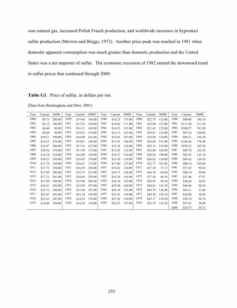
sour natural gas, increased Polish Frasch production, and worldwide increases in byproduct
sulfur production (Merwin and Briggs, 1972). Another price peak was reached in 1981 when
domestic apparent consumption was much greater than domestic production and the United
States was a net importer of sulfur. The economic recession of 1982 started the downward trend
in sulfur prices that continued through 2000.
Table G1. Price of sulfur, in dollars per ton.
[Data from Buckingham and Ober, 2001]
Year Current 2000$ Year Current 2000$ Year Current 2000$ Year Current 2000$ Year Current 2000$ 1900 $9.73 200.00 1920 $19.46 168.00 1940 $14.25 175.00 1960 $22.75 132.00 1980 $89.06 186.101901 $5.12 106.00 1921 $17.53 169.00 1941 $14.56 171.00 1961 $22.80 131.00 1981 $111.48 211.201902 $4.48 89.00 1922 $16.11 165.00 1942 $14.33 151.00 1962 $21.45 122.00 1982 $108.27 193.201903 $4.69 90.00 1923 $15.81 159.00 1943 $14.13 141.00 1963 $19.61 110.00 1983 $87.24 150.801904 $10.21 190.00 1924 $16.00 161.00 1944 $15.03 147.00 1964 $19.84 110.00 1984 $94.31 156.301905 $14.27 270.00 1925 $14.81 146.00 1945 $15.45 148.00 1965 $22.08 121.00 1985 $106.46 170.401906 $14.87 280.00 1926 $17.16 167.00 1946 $15.18 134.00 1966 $25.31 135.00 1986 $105.22 165.301907 $20.36 370.00 1927 $17.49 173.00 1947 $15.95 123.00 1967 $32.06 165.00 1987 $89.78 136.101908 $16.18 310.00 1928 $16.80 169.00 1948 $16.27 116.00 1968 $38.94 190.00 1988 $85.95 125.101909 $18.23 350.00 1929 $16.85 170.00 1949 $16.30 118.00 1969 $26.62 124.90 1989 $86.62 120.301910 $17.74 330.00 1930 $16.67 172.00 1950 $17.80 127.00 1970 $22.77 101.06 1990 $80.14 105.601911 $17.73 330.00 1931 $16.29 185.00 1951 $19.63 130.00 1971 $17.20 73.13 1991 $71.45 90.341912 $17.05 300.00 1932 $16.75 211.00 1952 $19.73 128.00 1972 $16.76 69.04 1992 $48.14 59.091913 $17.31 301.00 1933 $16.64 220.00 $24.26 156.00 1973 $17.56 68.10 1993 $31.86 37.971953
1954 197.00
$15.94 1937
247.00 $14.88
1914 $17.88 308.00 1934 $15.96 205.00 $24.19 155.00 1974 $28.43 99.30 1994 $30.08 34.951915 $16.61 283.00 1935 $15.69 1955 $25.49 164.00 1975 $44.91 143.70 1995 $44.46 50.241916 $15.72 248.00 1936 197.00 1956 $24.14 153.00 1976 $45.72 138.40 1996 $34.11 37.441917 $21.07 283.00 $16.16 193.00 1957 $21.91 134.00 1977 $44.38 126.10 1997 $36.06 38.691918 $21.65 1938 $14.54 178.00 1958 $23.38 139.00 1978 $45.17 119.30 1998 $29.14 30.781919 148.00 1939 $14.24 176.00 1959 $23.07 137.00 1979 $55.75 132.20 1999 $37.81 39.08
2000 $24.73 24.73
255

0
50
100
150
200
250
300
350
400
1900 1910 1920 1930 1940 1950 1960 1970 1980 1990 2000
YEAR
U.S
. SU
LFUR
PRI
CE
IN C
ONS
TANT
200
0 DO
LLAR
S PE
R M
ETR
IC T
ON
Price (elememtal sulfur ) Linear trend
Figure G2. U.S. sulfur price, in constant 2000 dollars, 1900-2000 (data from Buckingham and
Ober, 2001).
Domestic production
Over the last century elemental sulfur was mined using the Frasch process and recovered from
crude oil and natural gas. In the beginning of the 20th century, Herman Frasch invented the
superheated method of mining sulfur. In the Frasch process, sulfur is recovered from wells sunk
into salt domes by forcing heated water into the wells to melt the sulfur, which is then brought to
the surface. U.S. production of sulfur utilizing the Frasch process rose from 3,200 tons in 1900
256
to a production peak of 8.0 million tons in 1974 as shown in figure G3. Since then, it has
consistently declined, as recovered sulfur has become the main supplier of sulfur to the U.S.
economy. In 2000, sulfur production using the Frasch process was estimated as 900 thousand
tons (Ober, 2002) or 9 percent of domestic production as compared to 69 percent in 1974.
Sulfur is recovered during the processing of various products and fuels. These refining processes
reduce sulfur levels, in order to meet emission standards as part of pollutant abatement
regulations. The production of sulfur by this recovery process was practically nonexistent prior
to the 1940s. From that period forward, there was a steady increase in recovered production until
the early 1970s when new demands for fuels, specifically natural gas, dramatically increased the
rate at which production of recovered sulfur was advancing (figure G3). In 1940, production of
recovered sulfur was 4.0 thousand tons and by 1971, the production of recovered sulfur had
increased by over 400 times to slightly over 1.6 million tons. Petroleum refining and natural gas
processing continued their trend of increased sulfur production in 2000, with domestic
production reported at 8.38 million tons. From 1971 to 2000, recovered sulfur production, as a
percent of total sulfur production, gradually increased from approximately 17 percent to about 81
percent, replacing the Frasch process as the major supplier of sulfur in the United States (figure
G3).
257

Table G2. Domestic production of sulfur, in thousands of tons.
[Data from Buckingham and Ober, 2001]
Year Year Year Year Year 1900 86 1920 2,320 1940 3,680 1960 7,310 1980 12,0001901 1921 1,920 1941 4,030 1961 6,870 1981 10,2001902 208 1922 2,140 1942 3,140 1962 6,770 1982 9,3301903 233 1923 1,320 1943 3,940 1963 7,180 1983 10,5001904 334 1924 1,500 1944 4,490 1964 8,310 1984 11,6001905 402 1925 1,990 1945 4,550 1965 9,270 1985 11,1001906 297 1926 2,210 1946 5,170 1966 9,340 1986 10,6001907 475 1927 2,340 1947 5,630 1967 9,820 1987 10,8001908 368 1928 2,780 1948 5,490 1968 9,640 1988 11,5001909 351 1929 3,010 1949 6,020 1969 9,670 1989 11,5001910 306 1930 2,560 1950 6,210 1970 9,780 1990 10,8001911 1,020 1931 1,230 1951 6,380 1971 10,400 1991 10,7001912 782 1932 1,630 1952 6,370 1972 11,200 1992 10,9001913 708 1933 1,700 1953 6,760 1973 11,600 1993 11,5001914 840 1934 1,960 1954 7,050 1974 11,200 1994 11,5001915 1,030 1935 2,390 1955 7,900 1975 10,600 1995 11,8001916 1,600 1936 3,170 1956 7,070 1976 10,900 1996 11,8001917 1,910 1937 2,860 1957 6,300 1977 10,900 1997 12,0001918 1,640 1938 2,510 1958 6,280 1978 11,900 1998 11,6001919 1,630 1939 3,200 1959 6,750 1979 12,100 1999 11,300
2000 10,300
242
258
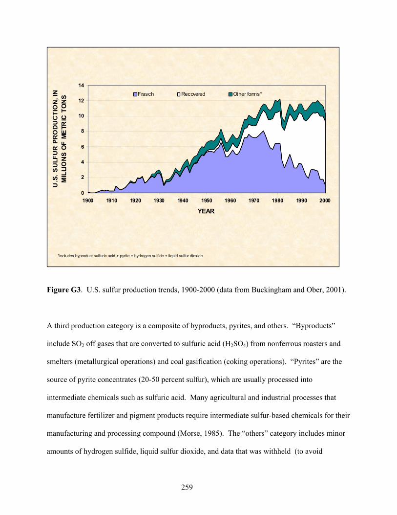
*includes byproduct sulfuric acid + pyrite + hydrogen sulfide + liquid sulfur dioxide
0
2
4
6
8
10
12
14
1900 1910 1920 1930 1940 1950 1960 1970 1980 1990 2000
YEAR
U.S
. SU
LFU
R P
RO
DU
CTI
ON
, IN
M
ILLI
ON
S O
F M
ETR
IC T
ON
S Frasch Recovered Other forms*
Figure G3. U.S. sulfur production trends, 1900-2000 (data from Buckingham and Ober, 2001).
A third production category is a composite of byproducts, pyrites, and others. “Byproducts”
include SO2 off gases that are converted to sulfuric acid (H2SO4) from nonferrous roasters and
smelters (metallurgical operations) and coal gasification (coking operations). “Pyrites” are the
source of pyrite concentrates (20-50 percent sulfur), which are usually processed into
intermediate chemicals such as sulfuric acid. Many agricultural and industrial processes that
manufacture fertilizer and pigment products require intermediate sulfur-based chemicals for their
manufacturing and processing compound (Morse, 1985). The “others” category includes minor
amounts of hydrogen sulfide, liquid sulfur dioxide, and data that was withheld (to avoid
259
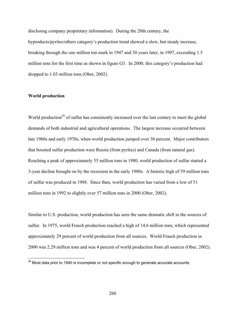
disclosing company proprietary information). During the 20th century, the
byproducts/pyrites/others category’s production trend showed a slow, but steady increase,
breaking through the one million ton mark in 1947 and 30 years later, in 1997, exceeding 1.5
million tons for the first time as shown in figure G3. In 2000, this category’s production had
dropped to 1.03 million tons (Ober, 2002).
World production
World production28 of sulfur has consistently increased over the last century to meet the global
demands of both industrial and agricultural operations. The largest increase occurred between
late 1960s and early 1970s, when world production jumped over 30 percent. Major contributors
that boosted sulfur production were Russia (from pyrites) and Canada (from natural gas).
Reaching a peak of approximately 55 million tons in 1980, world production of sulfur started a
3-year decline brought on by the recession in the early 1980s. A historic high of 59 million tons
of sulfur was produced in 1988. Since then, world production has varied from a low of 51
million tons in 1992 to slightly over 57 million tons in 2000 (Ober, 2002).
Similar to U.S. production, world production has seen the same dramatic shift in the sources of
sulfur. In 1975, world Frasch production reached a high of 14.6 million tons, which represented
approximately 29 percent of world production from all sources. World Frasch production in
2000 was 2.29 million tons and was 4 percent of world production from all sources (Ober, 2002).
28 Most data prior to 1940 is incomplete or not specific enough to generate accurate accounts.
260
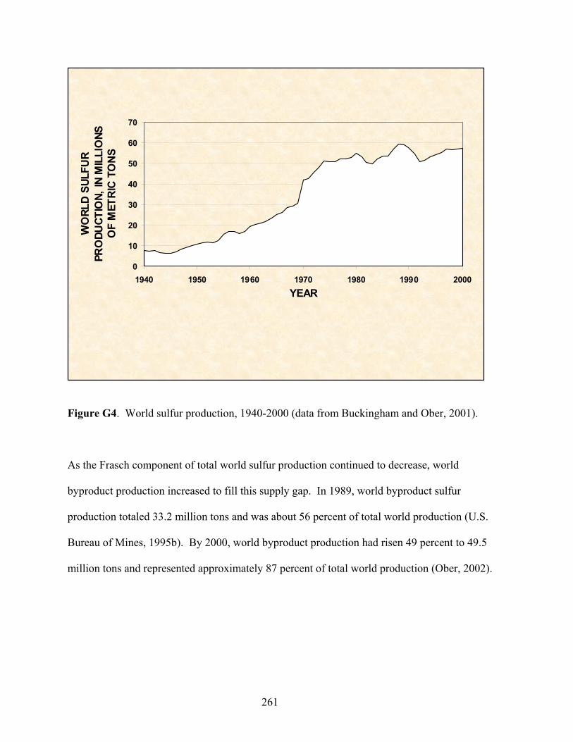
0
10
20
30
40
50
60
70
1940 1950 1960 1970 1980 1990 2000YEAR
WO
RLD
SULF
UR
PRO
DUCT
ION,
IN M
ILLI
ONS
O
F M
ETRI
C TO
NS
Figure G4. World sulfur production, 1940-2000 (data from Buckingham and Ober, 2001).
As the Frasch component of total world sulfur production continued to decrease, world
byproduct production increased to fill this supply gap. In 1989, world byproduct sulfur
production totaled 33.2 million tons and was about 56 percent of total world production (U.S.
Bureau of Mines, 1995b). By 2000, world byproduct production had risen 49 percent to 49.5
million tons and represented approximately 87 percent of total world production (Ober, 2002).
261
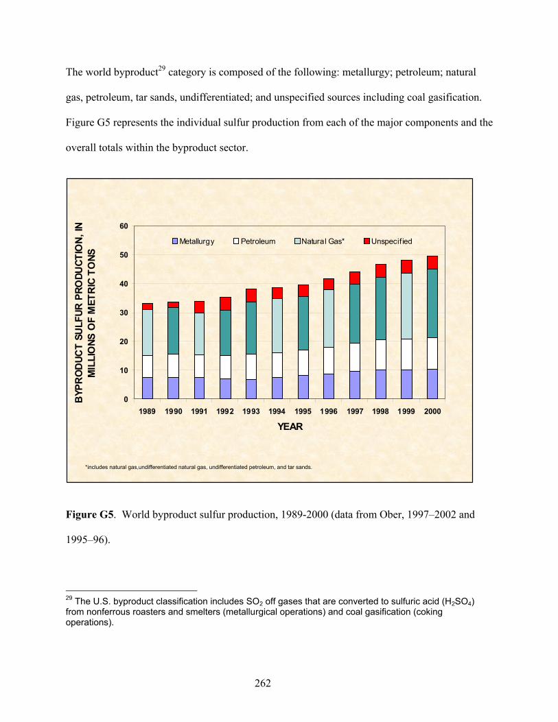
The world byproduct29 category is composed of the following: metallurgy; petroleum; natural
gas, petroleum, tar sands, undifferentiated; and unspecified sources including coal gasification.
Figure G5 represents the individual sulfur production from each of the major components and the
overall totals within the byproduct sector.
0
10
20
30
40
50
60
1989 1990 1991 1992 1993 1994 1995 1996 1997 1998 1999 2000
YEAR
BYP
RO
DUC
T SU
LFUR
PRO
DUCT
ION,
IN
MIL
LIO
NS O
F M
ETR
IC T
ONS
Metallurgy Petroleum Natural Gas* Unspecif ied
*includes natural gas,undifferentiated natural gas, undifferentiated petroleum, and tar sands.
Figure G5. World byproduct sulfur production, 1989-2000 (data from Ober, 1997–2002 and
1995–96).
29 The U.S. byproduct classification includes SO2 off gases that are converted to sulfuric acid (H2SO4) from nonferrous roasters and smelters (metallurgical operations) and coal gasification (coking operations).
262
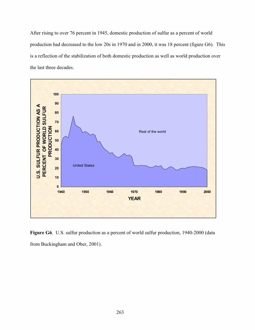
After rising to over 76 percent in 1945, domestic production of sulfur as a percent of world
production had decreased to the low 20s in 1970 and in 2000, it was 18 percent (figure G6). This
is a reflection of the stabilization of both domestic production as well as world production over
the last three decades.
0
10
20
30
40
50
60
70
80
90
100
1940 1950 1960 1970 1980 1990 2000
YEAR
U.S
. SUL
FUR
PRO
DUC
TIO
N AS
A
PERC
ENT
OF
WO
RLD
SU
LFUR
PR
ODU
CTIO
N
United States
Rest of the world
Figure G6. U.S. sulfur production as a percent of world sulfur production, 1940-2000 (data
from Buckingham and Ober, 2001).
263
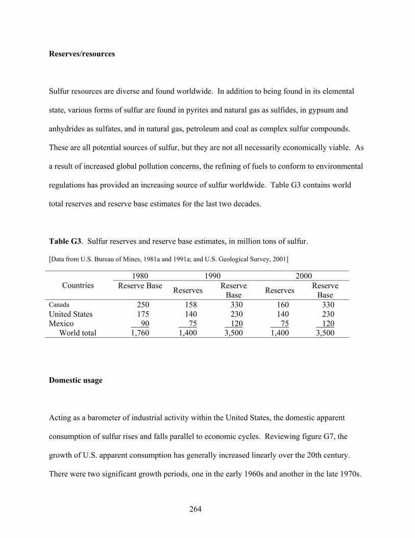
Reserves/resources
Sulfur resources are diverse and found worldwide. In addition to being found in its elemental
state, various forms of sulfur are found in pyrites and natural gas as sulfides, in gypsum and
anhydrides as sulfates, and in natural gas, petroleum and coal as complex sulfur compounds.
These are all potential sources of sulfur, but they are not all necessarily economically viable. As
a result of increased global pollution concerns, the refining of fuels to conform to environmental
regulations has provided an increasing source of sulfur worldwide. Table G3 contains world
total reserves and reserve base estimates for the last two decades.
Table G3. Sulfur reserves and reserve base estimates, in million tons of sulfur.
[Data from U.S. Bureau of Mines, 1981a and 1991a; and U.S. Geological Survey, 2001]
1980 1990 2000 Countries Reserve Base Reserves Reserve
Base Reserves Reserve Base
Canada 250 158 330 160 330 United States 175 140 230 140 230 Mexico 90 75 120 75 120 World total 1,760 1,400 3,500 1,400 3,500
Domestic usage
Acting as a barometer of industrial activity within the United States, the domestic apparent
consumption of sulfur rises and falls parallel to economic cycles. Reviewing figure G7, the
growth of U.S. apparent consumption has generally increased linearly over the 20th century.
There were two significant growth periods, one in the early 1960s and another in the late 1970s.
264
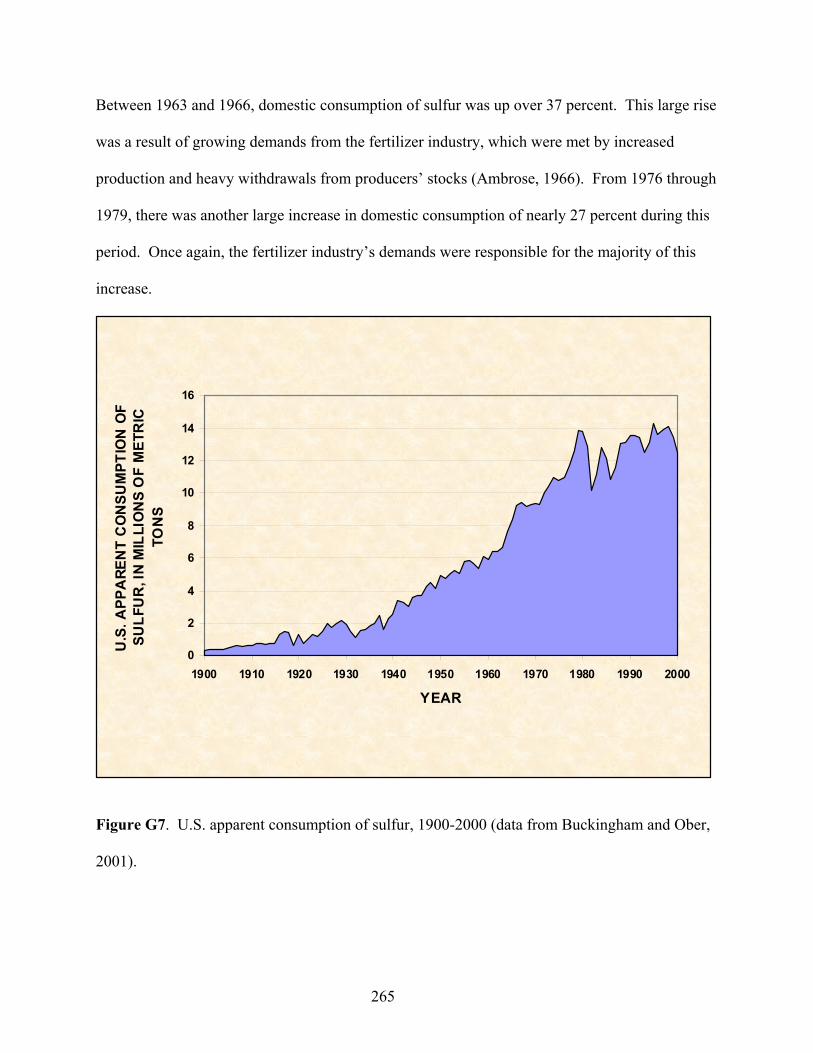
Between 1963 and 1966, domestic consumption of sulfur was up over 37 percent. This large rise
was a result of growing demands from the fertilizer industry, which were met by increased
production and heavy withdrawals from producers’ stocks (Ambrose, 1966). From 1976 through
1979, there was another large increase in domestic consumption of nearly 27 percent during this
period. Once again, the fertilizer industry’s demands were responsible for the majority of this
increase.
0
2
4
6
8
10
12
14
16
1900 1910 1920 1930 1940 1950 1960 1970 1980 1990 2000
YEAR
U.S
. APP
ARE
NT
CO
NSU
MPT
ION
OF
SULF
UR
, IN
MIL
LIO
NS
OF
MET
RIC
TO
NS
Figure G7. U.S. apparent consumption of sulfur, 1900-2000 (data from Buckingham and Ober,
2001).
265
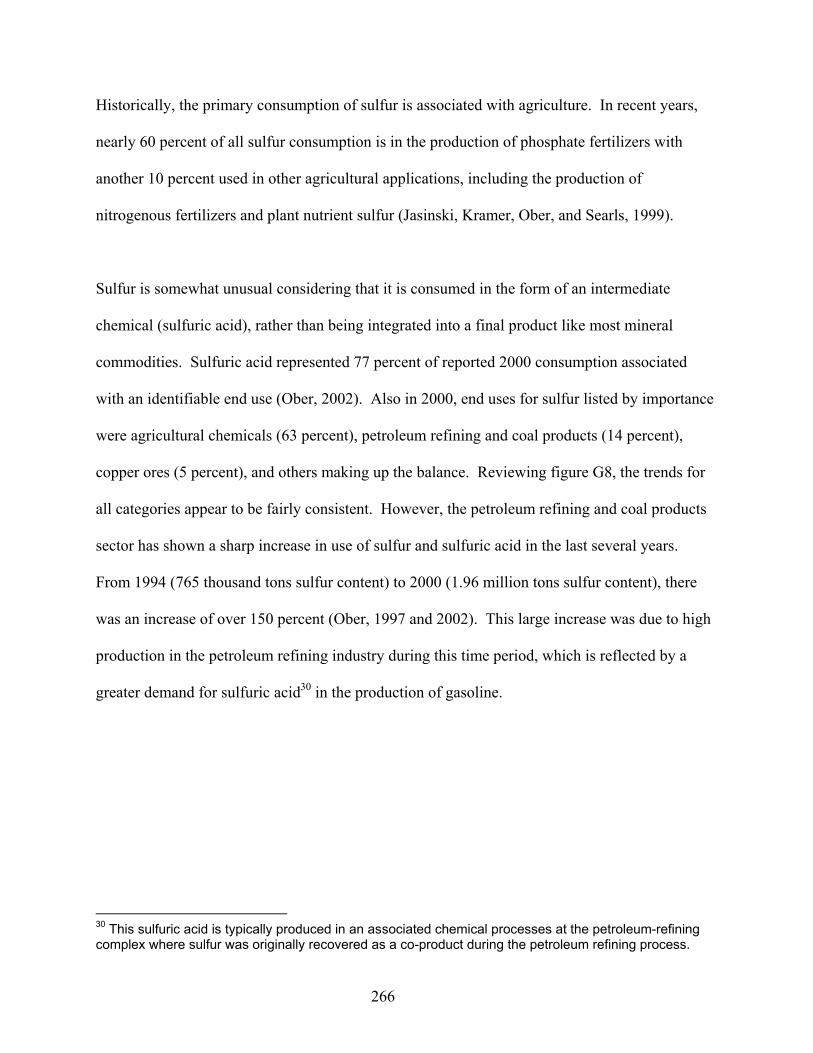
Historically, the primary consumption of sulfur is associated with agriculture. In recent years,
nearly 60 percent of all sulfur consumption is in the production of phosphate fertilizers with
another 10 percent used in other agricultural applications, including the production of
nitrogenous fertilizers and plant nutrient sulfur (Jasinski, Kramer, Ober, and Searls, 1999).
Sulfur is somewhat unusual considering that it is consumed in the form of an intermediate
chemical (sulfuric acid), rather than being integrated into a final product like most mineral
commodities. Sulfuric acid represented 77 percent of reported 2000 consumption associated
with an identifiable end use (Ober, 2002). Also in 2000, end uses for sulfur listed by importance
were agricultural chemicals (63 percent), petroleum refining and coal products (14 percent),
copper ores (5 percent), and others making up the balance. Reviewing figure G8, the trends for
all categories appear to be fairly consistent. However, the petroleum refining and coal products
sector has shown a sharp increase in use of sulfur and sulfuric acid in the last several years.
From 1994 (765 thousand tons sulfur content) to 2000 (1.96 million tons sulfur content), there
was an increase of over 150 percent (Ober, 1997 and 2002). This large increase was due to high
production in the petroleum refining industry during this time period, which is reflected by a
greater demand for sulfuric acid30 in the production of gasoline.
30 This sulfuric acid is typically produced in an associated chemical processes at the petroleum-refining complex where sulfur was originally recovered as a co-product during the petroleum refining process.
266
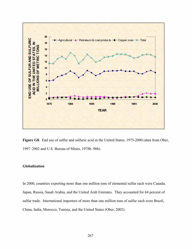
0
2
4
6
8
10
12
14
16
18
20
1975 1980 1985 1990 1995 2000
YEAR
END
USE
OF
SULF
UR A
ND S
ULFU
RIC
ACID
IN T
HE U
NITE
D ST
ATES
, IN
MIL
LIO
NS O
F M
ETRI
C T
ONS
Agricultural Petroleum & coal products Copper ores Total
Figure G8. End use of sulfur and sulfuric acid in the United States, 1975-2000 (data from Ober,
1997–2002 and U.S. Bureau of Mines, 1978b–96b).
Globalization
In 2000, countries exporting more than one million tons of elemental sulfur each were Canada,
Japan, Russia, Saudi Arabia, and the United Arab Emirates. They accounted for 64 percent of
sulfur trade. International importers of more than one million tons of sulfur each were Brazil,
China, India, Morocco, Tunisia, and the United States (Ober, 2002).
267
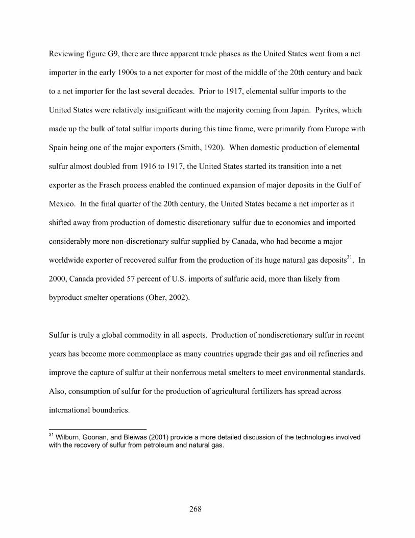
Reviewing figure G9, there are three apparent trade phases as the United States went from a net
importer in the early 1900s to a net exporter for most of the middle of the 20th century and back
to a net importer for the last several decades. Prior to 1917, elemental sulfur imports to the
United States were relatively insignificant with the majority coming from Japan. Pyrites, which
made up the bulk of total sulfur imports during this time frame, were primarily from Europe with
Spain being one of the major exporters (Smith, 1920). When domestic production of elemental
sulfur almost doubled from 1916 to 1917, the United States started its transition into a net
exporter as the Frasch process enabled the continued expansion of major deposits in the Gulf of
Mexico. In the final quarter of the 20th century, the United States became a net importer as it
shifted away from production of domestic discretionary sulfur due to economics and imported
considerably more non-discretionary sulfur supplied by Canada, who had become a major
worldwide exporter of recovered sulfur from the production of its huge natural gas deposits31. In
2000, Canada provided 57 percent of U.S. imports of sulfuric acid, more than likely from
byproduct smelter operations (Ober, 2002).
Sulfur is truly a global commodity in all aspects. Production of nondiscretionary sulfur in recent
years has become more commonplace as many countries upgrade their gas and oil refineries and
improve the capture of sulfur at their nonferrous metal smelters to meet environmental standards.
Also, consumption of sulfur for the production of agricultural fertilizers has spread across
international boundaries.
31 Wilburn, Goonan, and Bleiwas (2001) provide a more detailed discussion of the technologies involved with the recovery of sulfur from petroleum and natural gas.
268
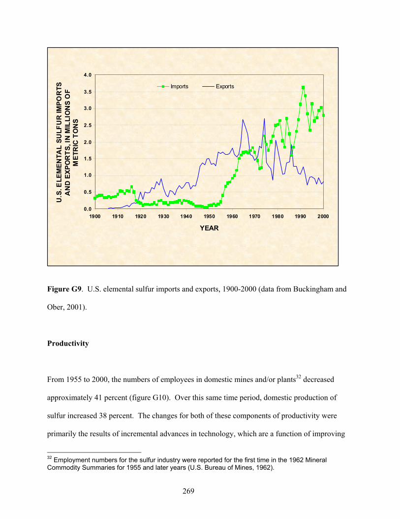
0.0
0.5
1.0
1.5
2.0
2.5
3.0
3.5
4.0
1900 1910 1920 1930 1940 1950 1960 1970 1980 1990 2000
YEAR
U.S
. ELE
MEN
TAL
SULF
UR
IMPO
RTS
A
ND
EXPO
RTS
, IN
MIL
LIO
NS
OF
MET
RIC
TO
NS
Imports Exports
Figure G9. U.S. elemental sulfur imports and exports, 1900-2000 (data from Buckingham and
Ober, 2001).
Productivity
From 1955 to 2000, the numbers of employees in domestic mines and/or plants32 decreased
approximately 41 percent (figure G10). Over this same time period, domestic production of
sulfur increased 38 percent. The changes for both of these components of productivity were
primarily the results of incremental advances in technology, which are a function of improving
269
32 Employment numbers for the sulfur industry were reported for the first time in the 1962 Mineral Commodity Summaries for 1955 and later years (U.S. Bureau of Mines, 1962).
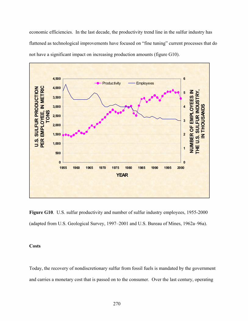
economic efficiencies. In the last decade, the productivity trend line in the sulfur industry has
flattened as technological improvements have focused on “fine tuning” current processes that do
not have a significant impact on increasing production amounts (figure G10).
0
500
1,000
1,500
2,000
2,500
3,000
3,500
4,000
4,500
1955 1960 1965 1970 1975 1980 1985 1990 1995 2000
YEAR
U.S
. SU
LFUR
PRO
DUCT
ION
PE
R E
MPL
OYE
E, IN
MET
RIC
TONS
0
1
2
3
4
5
6
NUM
BER
OF
EMPL
OYE
ES IN
TH
E U.
S. S
ULF
UR IN
DUST
RY,
IN T
HO
USA
NDS
Productivity Employees
Figure G10. U.S. sulfur productivity and number of sulfur industry employees, 1955-2000
(adapted from U.S. Geological Survey, 1997–2001 and U.S. Bureau of Mines, 1962a–96a).
Costs
Today, the recovery of nondiscretionary sulfur from fossil fuels is mandated by the government
and carries a monetary cost that is passed on to the consumer. Over the last century, operating
270
costs for discretionary sulfur varied greatly depending on factors such as size of operation,
deposit location, geology, and mining and processing methodology. Even though price is not the
same as cost, when cost data is not available, price data can be used as a crude proxy for costs.
However, it is important to keep in mind that other factors (such as profit) are also included in
the price, which is not included in the cost estimates. Therefore price is usually (but not
necessarily always) somewhat higher than costs. Current day domestic costs for mining pyrites
are not available because this source of sulfur is no longer economically competitive.
Conclusions
Over the last century, the most significant trend associated with elemental sulfur has been on the
supply side as discretionary mining of sulfur deposits has yielded to the nondiscretionary
recovery of sulfur from oil and natural gas refining. In addition, after being a major source of
sulfur at the beginning of the 20th century, global production of pyrites has almost been
eliminated because of related environmental and cost concerns.
Demand for sulfur, particularly for the manufacturing of agricultural fertilizers is expected to
continue throughout the world to help feed the ever-expanding global population. International
demand for sulfuric acid as an intermediate chemical should also continue as long as it maintains
its low cost profile in the chemical industry.
In the future, new applications may be developed that incorporate sulfur as a low cost raw
material. Thus, technological progress can provide additional markets for sulfur producers as
271

they face the potential global oversupply due to countries upgrading their manufacturing and
refining operations to eliminate sulfur-associated pollutants.
272
References
Ambrose, P.M., 1966, Sulfur, in Metals and Minerals: U.S. Bureau of Mines Minerals Yearbook 1965, v. I, p. 889-908. Buckingham, D.A., 1986, Availability of elemental sulfur and pyrite concentrate– Market economy countries: U.S. Bureau of Mines Information Circular 9106, 1986, 16 p. Buckingham, D.A., and Ober, J.A., 2001, Sulfur statistics, in Historical statistics for mineral commodities in the United States: U.S. Geological Survey Open-File Report 01-006. Jasinski, S.M., Kramer, D.A., Ober, J.A., and Searls, J.P., 1999, Fertilizers-sustaining global food supplies: U.S. Geological Survey Fact Sheet 155-99, September 1999, 4 p. Merwin, R.W., and Briggs, T.C., 1972, Sulfur, in Metals and Minerals: U.S. Bureau of Mines Minerals Yearbook 1971, v.I, p. 1119-1133. Morse, D.E., 1985, Sulfur, in Mineral Facts and Problems, 1985 edition: U.S. Bureau of Mines Bulletin 675, p. 783-797. Ober, J.A., 1992-96, Sulfur, in Metals and Minerals: U.S. Bureau of Mines Minerals Yearbook 1991-94, v. I. Ober, J.A., 1997-2002, Sulfur, in Metals and Minerals: U.S. Geological Survey Minerals Yearbook 1995-2000, v. I. Smith, P.S., 1920, Sulfur, in Nonferrous Metals: U.S. Geological Survey Mineral Resources of the United States, Part II, p. 301-308. U.S. Bureau of Mines, 1962a-96a, Mineral commodity summaries 1962-96: U.S. Bureau of Mines. U.S. Bureau of Mines, 1978b-96b, Minerals yearbook 1976-94: U.S. Bureau of Mines. U.S. Geological Survey, 1901, Mineral resources of the United States, 1900: U.S. Geological Survey, p. 829 - 842. U.S. Geological Survey, 1997-2001, Mineral commodity summaries, 1997-2001: U.S. Geological Survey.
273

274
Internet references cited Microsoft® Encarta® Online Encyclopedia , 2002, Sulfur, accessed July 19, 2002, at URL http://encarta.msn.com/find/concise.asp?ti=761560154&sid1.