The economic drivers of time-varyingcommodity market volatility*

Marcel Prokopczuk†,‡ and Lazaros Symeonidis�,�

January 15, 2013

Abstract

In this paper, we investigate the relationship between economic

uncertainty and commodity return volatility. Analyzing volatility for

the aggregate commodity market and for various commodity groups

we find that factors associated with macroeconomic and financial

market uncertainty explain subsequent volatility of commodity returns.

Variables motivated by commodity pricing theories, such as the futures

basis and hedging pressure, are also significant. Economic uncertainty

measures based on differences in beliefs of economic agents extracted

from survey data provide additional information to that contained

in volatility series of current economic fundamentals. Finally, we

find evidence of a strong bi-directional causal link between inflation

uncertainty and commodity return volatility. Our results have

important implications for economic policy making, asset allocation and

risk management.

JEL classification: G10, G12, G13, C22

Keywords: Commodities, macroeconomic uncertainty, realized volatility,

heterogeneity of beliefs.

*The authors would like to thank Claudio Morana, Bradley Paye and William Schwertfor helpful comments and clarifications. Contact emails: m.prokopczuk@icmacentre.ac.uk(Marcel Prokopczuk) and l.symeonidis@icmacentre.ac.uk (Lazaros Symeonidis).

�Zeppelin University, Am Seemooser Horn 20, 88045, Friedrichshafen, Germany�ICMA Centre, Henley Business School, University of Reading, Reading, RG6 6BA, UK.

1. Introduction

It is well known that asset return volatility is not constant. However, less is

known about the economic drivers of its variations. Starting with the seminal

paper of Schwert (1989), a large number of studies has challenged this issue

for equity and bond markets using a wide range of different variables and

techniques. In spite of their economic importance, commodity markets have

attracted much less attention in the literature. In this paper, we fill this gap by

investigating the links between time variation in commodity return volatility

and economic uncertainty.

There are numerous reasons for studying the economic drivers of commod-

ity price volatility. Unlike stocks and bonds, commodities are consumption

assets and input factors for the production process. Thus, any evidence from

equities should not be naively extrapolated to commodities. Moreover, prices

of commodities are important determinants of core macroeconomic concepts,

such as inflation, and therefore offer useful information to regulators and policy

makers. Understanding the forces that drive volatility of commodity returns

can also help investors improve their asset allocation decisions. In fact, the

impact of macroeconomic forces on commodity prices and their volatilities is

an issue of crucial importance for long term investors such as pension funds.

Furthermore, from an asset pricing perspective, recent findings suggest that

commodity risk is a priced factor in the cross-section of equity returns and,

as such, should be taken into account in asset pricing models (DeRoon and

Szymanowska, 2011).

We contribute to extant literature in multiple ways. To begin with, to

the best of our knowledge, we are the first to comprehensively study the

fundamental relationship between macroeconomic uncertainty and commodity

return volatility. Second, our study is the first to use survey expectations

data to quantify the impact of macroeconomic uncertainty on volatility of

commodity returns. We argue that this has important commodity pricing

implications. Third, although it is very important to test the causal

effect of the various economic variables on the volatility of commodity

returns, the possibility of causality going in the opposite direction, from

1

commodity markets to macroeconomic volatility, is also of great relevance for

economic policy makers. To this end, we analyze feedback effects between

macroeconomic uncertainty and commodity return volatility. Fourth, previous

studies are mainly based on indices, such as the GSCI or DJUBS to construct

commodity volatility proxies. However, most of these indices are dominated

by a particular group of commodities (e.g. energy in the case of the GSCI)

and therefore do not represent a well-diversified commodity portfolio that is

more appropriate for a fundamental analysis. Instead, our evidence is based

on an equally weighted and fully-collateralized commodity futures index in

the spirit of Gorton and Rouwenhorst (2006). Lastly, our analysis moves

beyond aggregate commodity volatility and assesses the behavior of different

commodity groups. Given the heterogenous nature of commodity assets, this

more detailed analysis can shed light on differences in behavior of particular

commodity groups (Erb and Harvey, 2006).

Our investigation leads to many interesting findings. Overall, our empirical

analysis suggests that macroeconomic uncertainty has an important effect

on commodity return volatility. Inflation uncertainty exhibits a consistently

positive and significant causal link with commodity return volatility. This

result holds for the majority of sectoral commodity portfolios and over the

various sub-samples considered. Additionally, we find that variables associated

with credit risk and money market stress, such as the default spread, TED

spread and the VIX are significantly related to subsequent commodity return

volatility in many cases. The latter observation is connected to the fact that

lower funding liquidity and greater equity market uncertainty implied by VIX

lead to higher volatility in financial markets (Brunnermeier and Pedersen,

2009).

Interestingly, we also find some evidence of a weakening role of fun-

damentals during the later part of our sample and especially after 2001.

This effect paired with the strong importance of financial risk factors, such

as those mentioned above, provides some indirect support for the view of

“financialization” in commodity markets. Tang and Xiong (2012) report

spillovers from financial to commodity markets as a result of the increased

2

participation of new institutional investors in commodity markets. Thus, our

results seem to corroborate their findings. Controlling for variables motivated

by commodity pricing theories, such as the interest-adjusted futures basis and

hedging pressure, we find that for some commodity groups these variables

bear significant explanatory power. In particular, futures basis leads to lower

volatility, while hedging pressure exhibits the opposite effect. This result can

be regarded as evidence that even though commodity markets have become

more integrated with financial markets, they are still segmented to some extent.

We also conduct a feedback analysis, which reveals a strong bi-directional

link between inflation uncertainty and commodity return volatility. This

bi-directional link is present over most sub-samples. Nevertheless, during the

recent period after the ’90s there is more evidence that commodity volatility

causes inflation volatility than the other way around. Furthermore, our

analysis shows that commodity return volatility helps to predict volatility of

real economic activity and exchange rates.

Constructing proxies of macroeconomic uncertainty based on the BlueChip

Economic Indicators survey, we obtain further evidence on the role of

macroeconomic uncertainty. Differences in beliefs of professionals regard-

ing short-term economic fundamentals have a strong effect on aggregate

commodity market volatility. Moreover, the macroeconomic uncertainty

measures based on survey expectations contain information additional to

that already contained in macroeconomic volatility estimates from historical

macroeconomic data.

Many researchers have examined the time variation in stock returns

with respect to macroeconomic conditions. The seminal paper by Schwert

(1989) analyzes the relationship between aggregate stock market volatility

and macroeconomic volatility and finds more evidence that equity volatility

causes macroeconomic volatility than the opposite. Subsequent studies

have suggested alternative methodologies aiming to better accommodate

the empirical behavior of the data. For example, Beltratti and Morana

(2006) document a bi-directional link between macroeconomic and equity

volatility by modelling structural breaks and long-memory of the volatility

3

processes. Engle et al. (2008) find that inflation and industrial production

predict aggregate S&P 500 volatility in the context of a new class of models

called Mixed Data Sampling (MIDAS)-GARCH, which make it feasible to

incorporate macroeconomic information in standard conditional volatility

models. Recently, Paye (2006, 2012) tests the in- and out-of-sample predictive

ability of various macroeconomic and financial factors for aggregate stock

market volatility. The author provides encouraging evidence regarding several

individual predictors although the overall performance of the models that

include economic variables is rather limited.

Most of the existing research on volatility of commodity prices, has focused

on factors specific to commodities, such as the value of the embedded option

in inventory (e.g., Deaton and Laroque, 1992; Ng and Pirrong, 1996; Geman

and Nguyen, 2005; Gorton et al., 2012, and many others) or the net positions

of investors (e.g., Bessembinder, 1992; De Roon et al., 2000). Furthermore,

studies that involve influences by economic variables are mainly concentrated

on commodity returns (Bailey and Chan, 1992; Hong and Yogo, 2012).

However, little effort has been made to explicitly relate commodity return

volatility to systematic risk. Recently, Christiansen et al. (2012) employed the

Bayesian Model Averaging approach to test the predictive ability of a large

number of variables on realized volatility of different asset classes including the

GSCI index for commodities. Our study focuses on the fundamental role of

economic uncertainty and its implications for volatility of commodity returns

rather than on finding the best predictors of future volatility in a large panel

of economic variables.

The remaining of this paper is organized as follows. Section 2 describes the

data and variables employed for our analysis. Section 3 analyzes volatility

measurement issues and the statistical properties of volatility estimates.

Section 4 presents empirical results. Section 5 discusses various robustness

checks and finally Section 6 concludes.

4

2. Data and variables

2.1 Commodity futures returns

We construct an equally weighted and fully-collateralized commodity futures

index following a methodology similar to Gorton and Rouwenhorst (2006). To

do this, we collect daily closing prices on first nearby futures contracts for a

large number of commodities traded in the US market and the London Metal

Exchange. Our data source is the Commodity Research Bureau (CRB). We

employ the entire history of daily prices available for each commodity futures

contract. The longest sample covers the period from July, 1959 to December,

2011. Where missing values are observed we apply a linear interpolation.1

The 33 commodities included in our index can be classified in four different

categories: (i) Agricultural (grains and soft commodities), (ii) Livestock, (iii)

Energy and (iv) Metals (industrial and precious metals). Table 1 lists the

commodity contracts included in the index along with the exchange where

they are traded and their introduction date to the index.

To construct the index we first take the price of the first nearby futures

contract for each commodity, assuming it expires on the first day of the

delivery month (rollover date). We assume that the position in futures is

fully-collateralized, which means that for each dollar invested into futures an

equal amount is invested in the risk-free asset. Therefore the so called “total

return” on each individual futures contract is computed as:

ri,t =Fi,t,TRf,t

Fi,t−1,T

− 1 (1)

where: Fi,t,T is the day t price of the futures contract on commodity i, maturing

at T , and Rf,t is the gross daily return on the risk-free asset. As risk-free rate

we use the yield on the 3-month T-bill obtained from the Federal Reserve at

St Louis.

The return corresponds to a rollover strategy according to which we keep a

position on the nearest to maturity contract until the first day of the delivery

1We also experimented with other interpolation methods, in particular spline and cubicapproaches. The resulting index was not affected by the particular interpolation method.

5

month when the position is changed to the next to maturity contract. Prior

to the rollover day, the return on the position comes exclusively from the day-

to-day changes in the futures price (also termed spot return) plus the return

on the collateral (T-bill). On the rollover day, the previous position is closed

by selling the expiring contract and immediately buying the next to maturity

contract. This leads to an additional return, known as “roll return”, which is

positive when the term structure is downward sloping (“backwardation”) and

negative when it is upward sloping (“contango”). Therefore, the return on the

rollover day is the sum of the spot return, the roll return and the return on

the collateral.2 Finally, we construct the aggregate commodity index as an

equally weighted average of the daily returns across all available commodities

on a particular day.3

Figure 1 illustrates the evolution of the equally weighted aggregate

commodity futures index for the entire sample period from July, 1959 to

December, 2011. From the figure one can easily observe the increase in

commodity prices that started gradually in 2003 and peaked during 2006-2008.

This period of steep increase in prices of most commodities from 2006 to

2008 is usually referred to as the “commodity price boom period” (Haniotis

and Baffes, 2010). The driving factors of this escalation in commodity prices

during the aforementioned period is an open research question (e.g., Singleton,

2013, for the oil market). As a robustness check and in order to ensure

that our analysis is not sensitive to the use of the particular commodity

futures index constructed above, we also include the exchange traded Goldman

Sachs Commodity Index (GSCI) to represent the aggregate commodity market.

However, the fact that this index is dominated by energy commodities may

obscure our fundamental analysis and therefore we compute daily returns of

this index as the equally weighted average of returns across its sub-indices.

We denote this index by GSCI(Eq) to distinguish it from the standard GSCI

index.

2For more technical details on the construction of the index and on potential issues withsurvivorship biases the interested reader can refer to Gorton and Rouwenhorst (2006).

3Note that the number of commodities included in the index changes over time dependingon the availability of price data. Therefore, the index starts with 9 commodities in 1959 andends up with 33 in 2011.

6

2.2 Explanatory variables

1. Macroeconomic variables

We collect a set of economic series to construct proxies of macroeconomic

uncertainty. These series include: CPI inflation, industrial production

growth, M2 money supply growth, 3-month T-bill yield, the yield on 10-year

government bond and the return of the trade-weighted US dollar index against

major currencies. The first three variables are available at monthly frequency,

whereas the other three are sampled daily. All data were obtained from the

Federal Reserve Bank of St Louis (FRED).

2. Financial variables

In addition to the previous macroeconomic variables we consider a number of

financial variables.4 First, we compute daily returns on the S&P 500 using

daily prices collected from Bloomberg. Second, we obtain monthly average

yields on Moody’s Aaa and Baa-rated corporate bonds from FRED. Moody’s

Aaa (Baa) corporate bond yield represents an index of the performance of

all bonds rated as Aaa (Baa) by Moody’s Investors Service. Additionally, we

consider four variables related to debt market risk, namely: (i) the default

spread defined as the difference between the Moody’s Baa and Aaa corporate

bond yields, (ii) the term spread defined as the long term government bond

yield minus the T-bill yield, (iii) the default return spread, defined as the

difference between the long term corporate and the long term government

bond returns, and (iv) the TED spread defined as the difference between the

3-month LIBOR rate and the 3-month T-bill. All four variables above are

monthly. The data are from FRED except for the corporate and government

bond returns that are obtained from the online appendix of Goyal and Welch

(2008). Monthly yields correspond to averages from daily values.

Finally, we consider the end-of-month level of the VIX, which represents

investors’ expectations on the 30-day ahead volatility extracted from

4We should point out here that some of the variables in the macroeconomic group, couldhave also been classified as financial variables, e.g. the T-bill yield, the yield on the 10 yearbond.

7

out-of-the-money call and put options (for further details see CBOE website).

Moreover, VIX is often regarded as a proxy of general economic uncertainty

(Connolly et al., 2005) or investor’s sentiment (Baker and Wurgler, 2007).

3. Commodity-specific variables

We construct aggregate measures of variables that are central to fundamental

commodity pricing theories, namely the theory of storage and the theory of

normal backwardation. Specifically, we focus on aggregate measures of: (i) the

commodity futures basis, (ii) the growth of open interest in commodity futures

and (iii) the hedging pressure of commercial and non-commercial traders,

respectively.

Regarding the aggregate futures basis, we use monthly observations on

the first and second nearby contracts. The former (latter) is treaded as spot

(futures) price. The source is the CRB as above. We first calculate the monthly

interest-adjusted basis for each commodity i as follows:

bi,t =Fi,t,T2 − Fi,t,T1

Fi,t,T1

− rf,t (2)

where: Fi,t,T2 is the price in month t of a futures contract on commodity

i maturing at T2, Fi,t,T1 is the price in month t of the first nearby futures

contract maturing at T2 (T2 > T1) and rf,t is the monthly T-bill rate serving as

a proxy for the risk-free rate. Based on the cost-of-carry relationship it follows

that the above measure of the commodity futures basis represents storage

costs and convenience yields (Ng and Pirrong, 1994). Next, we compute the

median of the basis (less sensitive to outliers compared to the mean) across

all commodities within a specific sub-index. These series serve as the basis

measures for each commodity sector. Finally, to obtain a proxy for the adjusted

basis of the aggregate commodity market, we take the average basis across all

four sectors (agricultural, animal, energy and metals).

For the open interest variable, we first collect monthly spot price data for

all commodities in our equally weighted portfolio from the CRB. Next, we

obtain end-of-month data on the open interest in futures from the webpage

8

of the Commodity Futures Trading Commission (CFTC). The dataset covers

the period from January, 1986 to December, 2011. We should point out that

certain commodities in our index are not covered by the CFTC dataset, such

as, for example, the metals traded at the LME.

To construct the open interest variable we closely follow the procedure

described in Hong and Yogo (2012). In particular, we first compute the open

interest in monetary terms for each commodity as the product of spot price

times the end-of-month open interest. Then, for each of the four sub-indices

considered, we add up the dollar open interest across all commodities in

the particular sub-sector and compute its logarithmic growth. Finally, the

aggregate open interest measure for the whole market is obtained by taking

the median across all commodity sub-indices. As pointed out by Hong and

Yogo (2012), the open interest proxies are very noisy. Therefore, similar to

the aforementioned study, we smooth the final open interest series by taking

a 12-month geometric average.5

A prominent stream of the literature in commodity futures pricing

supports the notion that risk premia vary with the net positions of hedgers

(Bessembinder, 1992; De Roon et al., 2000). Also, recent studies provide

evidence that positions of particular types of traders (e.g. hedge funds) have a

significant impact on commodity price volatility (Buyuksahin and Robe, 2010).

Motivated by these considerations, we include a measure of aggregate hedging

pressure in the commodity market in our analysis. The CFTC reports contain

the short and long positions of commercial and non-commercial traders for

each month. Commercial traders are widely regarded as hedgers (De Roon

et al., 2000) while non-commercial traders as speculators. Using these data we

compute the hedging pressure for each commodity sector and over each month

as follows:

HPt =

N∑i=1

(Shorti,t − Longi,t)

N∑i=1

(Shorti,t + Longi,t)

(3)

5To cross-check our constructed proxies, we download the relevant series from the onlineappendix of Hong and Yogo (2012). The final series look very similar even though thecommodities included in our and their indices are not exactly the same.

9

The above definition simply refers to a ratio of the sum of short minus long

positions within a particular sector over the total number of positions (in US

dollars) for all commodities in each particular sector (agricultural, energy,

livestock, metals). Finally, a measure of hedging pressure for the whole

commodity market is obtained as the average hedging pressure across the four

sectors (similar to Hong and Yogo, 2012). Furthermore, following exactly

the same steps we create a measure of speculative pressure defined as the

negative (long minus short) of the above variable and employing the positions

of non-commercial traders.

3. Measuring volatility

Following French et al. (1987) and Schwert (1989) a proxy for commodity

market volatility of month t is computed as the square root of the sum of daily

squared returns. This measure is represented as follows:

RVt =

√√√√ Nt∑j=1

r2j,t (4)

where: rj,t is the return on day j of month t in excess of the mean return of

this month and Nt the number of daily return observations in month t. This

measure is widely known as realized volatility. We also use this volatility proxy

for the returns of the sectoral indices of the equally-weighted index.

The above method of computing volatility exhibits several advantages.

First, it is model-free and easy to compute. Second, as pointed out in Andersen

et al. (2003) and Barndorff-Nielsen and Shephard (2002), under appropriate

conditions realized volatility is an unbiased estimator of the true volatility

process. We also compute realized volatility for those macroeconomic and

financial series that are sampled at daily frequency, namely: S&P 500 returns,

T-bill yields, 10 year government bond yields and the returns on the US dollar

trade-weighted exchange rate index.

Nonetheless, many of the macroeconomic series are available only at

monthly frequency. Therefore, in these cases, we cannot rely on the above

10

estimator to obtain realized volatility. Methodologies to obtain volatility

estimates for low frequency data can be distinguished between parametric (e.g.

multivariate/univariate GARCH models) and non-parametric (e.g., Schwert,

1989; Bansal et al., 2005). In our study, we follow the non-parametric two-step

method of Schwert (1989). The first step of the method involves estimation

of a 12th order autoregressive model (AR(12)) on the logarithmic difference of

the series, including dummy variables to allow for different monthly intercepts,

as follows:

Rt =12∑i=1

aiMi +12∑i=1

biRt−i + et (5)

where: Rt is the first order difference between the natural logarithm of the

series (or simply the yield for interest rate instruments) and Mi are monthly

dummy variables. In the second step, an AR(12) model is fitted on the absolute

values of the residuals from the first step, including again dummy variables to

allow for different monthly intercepts:

|et| =12∑j=1

γjMj +12∑j=1

δi|et−i|+ at (6)

The absolute values of the residuals from Equation (5) correspond to realized

volatility estimates of the series (or equivalently unconditional volatility).6

Relative to the squared residuals, for example in a GARCHmodel, the absolute

value has the advantage that it is less skewed and also less sensitive to outliers.

On the other hand, the fitted values from the second step represent

realized volatility predictions of month t conditional on information available

up to month t-1. In other words, these predictions are conditional volatility

estimates given information available at t-1. This is based on a similar idea

to the GARCH models of Engle (1982) and Bollerslev (1986). For a detailed

discussion on volatility measurement methods see Andersen et al. (2002). The

two-step algorithm above is applied to the following series: CPI inflation,

industrial production growth (IP), M2 money supply growth and Moody’s

6Similar to Schwert (1989), the absolute values of the residuals from the first stepare multiplied by

√π/2 since the expectation of the absolute value is smaller than the

expectation of the normal distribution that the error term is assumed to follow.

11

Aaa corporate bond yield.7

The second step of Schwert’s method is also estimated for variables

sampled daily in order to obtain conditional volatility series for those as

well. In this case, we simply replace the absolute errors in the second

step with the realized volatility series obtained from Equation (4). In our

subsequent empirical analysis, we always employ these conditional volatility

series (volatility predictions) as economic uncertainty proxies (explanatory

variables) similar to (Schwert, 1989; Paye, 2012). It is necessary to point

out here that for the VIX as well as for the debt market variables, namely the

term spread, the default spread, the default return spread and the TED spread

we directly work with these series rather than volatilities since they already

express risk.

3.1 Statistical analysis of volatility estimates

Figure 2 illustrates kernel density plots of realized volatility estimates for the

equally-weighted commodity index and GSCI(Eq) index, respectively. Looking

at the top panel of this figure, which refers to the level of realized volatility, we

see that the series of realized volatilities of both indices are positively skewed

and highly leptokurtic. These non-Gaussian characteristics of the empirical

distribution of volatility estimates may lead to non-normal errors in the linear

regression models employed for our analysis. To this end, we choose to work

with the logarithm of annualized realized commodity return volatility, defined

as: RVt = log (√12RVt). Andersen et al. (2003) point out that although

the distribution of raw volatility estimates is rightly-skewed, the logarithmic

volatility distribution is close to normal. The bottom panel of Figure 2 that

illustrates the kernel density plots of logarithmic realized commodity market

volatility confirms this conjecture.

Table 2 presents diagnostic statistics for the regressions of Equation (6)

used to obtain conditional volatility estimates. As already mentioned above

the dependent variable in Equation (6) corresponds to realized volatilities

7The Moody’s Aaa corporate bond yield is also available daily from FRED. However,the daily series begins only in 1983, which is a too short period for our study. Therefore, wechoose to proceed with the monthly series.

12

computed by Equation (4) for variables sampled daily and by Equation (5)

for variables sampled monthly. In the third column of the table we report

the sum of the autoregressive coefficients that capture the persistence of the

realized volatility process together with the t-statistic for the hypothesis that

this sum is equal to unity (integrated volatility). Except for inflation volatility,

all other series of volatility estimates exhibit a high degree of persistence, since

the sum of autoregressive coefficients is higher close to 0.8 or higher in most

cases. Therefore, the hypothesis of non-stationary (integrated) variance is

rejected in all cases suggesting mean-reverting volatility processes. The fourth

and fifth columns contain F-statistics with their associated p-values from the

following two tests: i) all seasonal dummies are equal, and ii) all autoregressive

coefficients are jointly zero. The F-test indicates rejection of the null hypothesis

in all cases. Therefore, the selected approach of obtaining volatility proxies

appears appropriate. Finally, the table reports the Ljung-Box statistic for

serial correlation up to 24 lags, which evaluates the adequacy of the model.

The statistic suggests rejection of the null hypothesis of autocorrelation in

model residuals, which shows that the AR(12) model adequately captures the

persistence of the volatility series and also removes most of the autocorrelation

in the series.

In Figure 3 we plot the time series of conditional volatility series of the

equally weighted commodity index against each conditional macroeconomic

volatility series. To make the plots easier to read, we standardize all

volatility series. These graphs reveal some interesting patterns concerning

the relationship between macroeconomic and commodity return volatility.

First, commodity market volatility is much higher compared to macroeconomic

volatility. Second, there is a clear co-movement between commodity and

macroeconomic volatility during the period that coincides with the financial

crisis and the commodity price boom period. Furthermore, among the

macroeconomic volatility series, inflation seems to be the most highly

correlated with commodity return volatility.

Table 3 displays Spearman’s rank order correlations between predictions of

aggregate commodity market volatility and predicted volatilites of macroe-

13

conomic variables and financial variables. We report correlations for the

period 1970-2011, which corresponds to the full sample period employed

for our subsequent estimations, and for the sub-period, 1991–2011. We see

that most correlation coefficients are positive and significant at the 5% level.

This suggests that higher volatility of commodity returns is associated with

higher macroeconomic and financial market volatility and vice versa. Overall,

inflation volatility exhibits the highest correlation with commodity market

volatility, around 50%, while correlation between commodity and equity return

volatility is around 30%. Correlation of aggregate commodity return volatility

with the other macroeconomic volatility series is generally low for both the

full sample period and the sub-period considered. A notable exception is the

correlation with the US exchange rate index volatility for the period 1991-2011,

which is equal to 45%.

3.2 Summary statistics of explanatory variables

Table 4 reports summary statistics for the variables used in our empirical

analysis that follows. Commodity-specific variables are not reported due to

space limitations. Inspection of the table shows that historical equity market

volatility and option implied volatility (VIX), are by far the most volatile

series, followed by long term bond return volatility and US dollar index

volatility. This observation is consistent with previous studies which showed

that financial volatility is generally much higher than macroeconomic volatility

(Schwert, 1989; Beltratti and Morana, 2006). The first order autocorrelation

coefficients are positive and large for most series especially for those associated

with interest rates and bond yields, such as the default spread or the T-bill

yield. The twelfth order autorocorrelation coefficients are also large in many

cases although much lower than the corresponding first order coefficients. This

slow decay in autocorrelations suggests relatively high persistence of the series.

To ensure that this high persistence is not related to non-stationary series

that could potentially cause inference problems in our estimations, we perform

Phillips-Perron (Phillips and Perron, 1988) unit root tests for each series. The

test statistics and their associated p-values (MacKinnon, 1994) reject the null

14

hypothesis of a unit-root at the 1% significance level for all series. Therefore,

in the first place, we do not need to employ alternative econometric procedures

(e.g., Integrated Moving Average processes).

4. Empirical results

In our empirical analysis, we investigate the links between time variation

in commodity return volatility and macroeconomic and financial market

uncertainty. To this end, we consider a number of economic and financial

variables to test whether they explain subsequent return volatility of the

aggregate commodity market and of various commodity sectors. Given

the role of idiosyncratic risk in commodity markets, we also control for

commodity-specific factors, such as the futures basis and the positions of

hedgers/speculators. First, we analyze the behaviour of commodity market

volatility over the business cycle. Second, in a univariate regression context,

we analyze the ability of each individual variable to offer explanatory power

beyond that contained in lags of volatility. Third, we extend the analysis

to a multivariate framework that incorporates multiple factors. After this,

we explore the impact of heterogeneity in beliefs about term economic

conditions of professional forecasters on commodity return volatility. Finally,

we investigate causality between macroeconomic uncertainty and commodity

market volatility with a VAR analysis.

4.1 Commodity market volatility during recessions

Commodity futures prices vary across the business cycle. Fama and French

(1988) analyze this issue for metals, while Gorton and Rouwenhorst (2006)

document that commodity assets exhibit a slightly different exposure to

business cycle conditions relative to stocks and bonds. In particular, they

report that commodity returns tend to be higher on the onset of a recession

whereas they become negative during later stages of a recession when stock

and bond markets begin to recover. Below, we investigate the behaviour

of commodity return volatility over the business cycle. Our longest sample

15

period (1959-2011) covers seven recession periods according to the NBER

classification.

Figure 4 plots the natural logarithm of realized volatility of the equally

weighted index and the GSCI(Eq) index, respectively. Super-imposed on the

graph are the NBER recession months. Inspection of this plot shows that

commodity market volatility tends be higher during recessions. However, some

additional remarks apply. First, the increase in volatility is not systematically

documented during all recessions. For instance, during the recession of 2001,

following the dot.com bubble, the volatility hardly changed. Second, although

volatility of commodity returns tends to be higher during recessions, in many

cases the volatility is not substantially higher compared to highly volatile

episodes not associated with recessions. This fact highlights the role of

non-systematic (idiosyncratic) risk factors that affect the supply and demand

of commodity prices, e.g. geopolitical events.

To formally test the behaviour of commodity return volatility over the

business cycle more formally, we estimate the following regression:

RVi,t = a+6∑

i=1

biRVi,t−i + γ · INBER,t + ut (7)

where: RVi,t is the realized volatility of commodity return index i in month

t and INBER,t is a dummy variable that takes the value of 1 for NBER

recession months and 0 otherwise. We include six lags of realized volatility

in the right side of Eq. (7) to account for persistence in volatility and avoid

spurious inference (Paye, 2006). If the coefficient of the business cycle dummy

is significantly different from zero means that the volatility of the series is

higher on average during recessions. The regression is estimated for the equally

weighed commodity index and its four sub-indices as well as for the GSCI index

(equally weighted). The energy portfolio is excluded from the estimations since

its price history is too short (1983-2011) for this analysis. In addition, we also

estimate the above regression for the macroeconomic and financial volatility

series.

Table 5 reports the estimation results. The coefficient of the recession

16

dummy is positive and strongly significant for both the equally weighted index

and for the GSCI(Eq) index. This result suggests that during recessions

aggregate commodity market volatility is higher on average. Inspecting the

individual commodity groups, we observe that volatility is significantly higher

for metals, but not for agricultural and livestock portfolios. The last column

of the table reports the percentage increase in volatility during recessions

compared to expansions. These volatility increases are quite large in most

cases. Furthermore, S&P 500 returns, inflation, industrial production and

money supply exhibit substantial increase in volatility during recessions. There

is relatively weaker evidence for interest rates, FX rates and corporate bond

yields.

These results supports the view that volatility of commodity returns is

strongly affected by real economic conditions. An interpretation for this is

that shifts in investors’ risk aversion during recessions may induce time-varying

patterns in expected returns and therefore rime variation in return volatility.

4.2 Evidence from univariate estimations

We begin by estimating the following specification on the logarithm of

commodity return volatility:

RVt = a+ γXi,t−1 +6∑

j=1

βj˜RVt−j + ut (8)

where: RVt is the natural logarithm of realized commodity return volatility in

month t and Xi,t−1 is the scalar value of variable i in month t− 1. The above

specification refers to one-by-one regressions against each variable. Newey-

West (1987) standard errors (with 12 lags) are employed for the estimations.8

Given the persistent nature of volatility, its own lags already capture a rich

set of information about current volatility. Therefore, for a variable to be

characterized as a significant indicator of future volatility, it should provide

information additional to that already contained in lagged volatility.

8Experimentation with higher lags (15 and 18 respectively) yield very similar t-statistics.

17

We estimate the above set of regressions for six different dependent

variables: the logarithm of realized volatility of the equally weighted

commodity futures return index, its four equally weighted sub-indices, and

the realized volatility of the GSCI index adjusted for equal weights. Prior

to 1970, our index consists only of few commodities (around 10), most of

them agricultural. As a consequence, the index is not well-diversified since

it is dominated by a single sector. Moreover, our price history for GSCI

index begins in 1970. Therefore, we chose to start our analysis from January

1970 although for the previous business cycle analysis we employed the full

history of data. Our estimations are performed on the entire sample spanning

1970-2011 and also on various sub-periods of this sample. One way to assess

the economic significance of a specific variable is through the increase in the

adjusted R2 after adding the variable in the plain AR(6) specification (also

called the benchmark).

Tables 6 to 11 summarize the results of estimating the above six sets of

regressions. All variables, including the dependent, are standardized prior to

the estimations by subtracting the sample mean and dividing with the sample

standard deviation to facilitate better comparability across coefficients. A

first look on the results across sub-samples and sectoral commodity indices,

reveals that some variables consistently enter with significant coefficients.

Inflation volatility appears to be the most significant individual predictor in

economic and statistical terms. Moreover, factors related to financial market

conditions, such as the default return spread, the term spread or the VIX

offer explanatory power for many portfolios and sub-periods. Controlling for

commodity-specific factors, we observe that these are significant determinants

of commodity return volatility in many cases, while their signs are consistent

with theoretical predictions.

We observe some evidence of time variation in the response of commodity

return volatility to the various economic factors across the different commodity

groups. This is, to some extent, expected due to the heterogeneous nature of

commodity assets. For example, some of them are primary consumable goods

(e.g. grains), some others are inputs in the production process, e.g. lumber,

18

or behave more like financial assets, e.g. gold.

Looking at the results of the aggregate commodity market indices (Tables 6

and 11, respectively), we see that inflation volatility is highly significant at the

1% level for the whole sample period of 1970–2011. Its sign suggests a positive

impact on short term volatility of commodity returns. This positive effect

may be related to the higher trading activity in commodities during periods

of high inflation uncertainty since they are widely considered as good a hedge

against inflation (Edwards and Park, 1996). In the 2001–2011 sub-period,

which includes the recent commodity price boom, the significance and the

magnitude of the impact of inflation uncertainty seems to weaken.

In contrast, the importance of some financial factors, such as the default

return spread, TED spread and VIX becomes greater in the sub-sample

after 2000. This may provide some indirect support for the argument of

“financialization” according to which commodity markets are becoming more

integrated with traditional financial markets due to the participation of new

investors (e.g. hedge funds). As a consequence of the financialization process

the dependence of commodity prices on factors specific to stocks or bonds

has increased (Silvennoinen and Thorp, 2010). The coefficients of both the

VIX and TED spread are positive suggesting that greater values for these

variables are associated with more volatile commodity returns. This positive

effect for the VIX can be understood if one thinks that it represents investors’

attitude to risk and as such it also provides signals about other risky assets,

like commodities. On the other hand, the TED spread is a proxy for funding

liquidity (Brunnermeier et al., 2008) and higher values of this variable are

linked to higher illiquidity. Hence, the dry up in liquidity during the recent

financial crisis pushed volatility higher. This shows that the VIX and TED

spread have the same effect on commodity return volatility. Brunnermeier

et al. (2008) reach a similar conclusion for currency returns.

Concerning the variables motivated by commodity pricing theories, we

observe that the measure of aggregate commodity futures basis, although

insignificant in the entire sample period, enters with a highly significant

and large in absolute value coefficient in the second half of the sample

19

(1991–2011). Its sign is negative and consistent with the predictions of the

theory of storage (Ng and Pirrong, 1994; Gorton et al., 2012). Furthermore,

the effect of aggregate hedging pressure is positive for aggregate commodity

market volatility and significant at the 5% level, while its sign suggests that

volatility increases with higher hedging demand. This is in line with evidence

of other studies which examine the impact of hedgers’ positions on volatility

of commodity returns (Buyuksahin and Robe, 2010; Silvennoinen and Thorp,

2010). Speculative pressure, on the other hand, is important only in the period

after 2000. This, however, highlights the potential role of speculation in the

recent commodity price boom during 2008, which was also accompanied by

increased price volatility (see Figure 4). The conclusions are very similar and

in many cases identical for the GSCI(Eq) index, enhancing the robustness of

our evidence.

As already mentioned above, the estimation results suggest cross-sectional

differences in the explanatory power afforded by the various variables. For

instance, a look on the results of agricultural volatility shows that for the first

half of the sample (1970–1990) only inflation volatility and the futures basis

enter with significant coefficients. However, in the second half of the sample

(1990–2011) several other variables become important, such as equity return

volatility, the default spread, the term spread, the VIX, etc. In contrast, for

metals the only common important factor during the 1991–2011 sub-period is

inflation volatility, whereas from the rest of variables hedging and speculative

pressure exhibit significant coefficients at the 1% level. Default return spread,

the futures basis and interest rate volatility seem to matter as explanatory

factors for energy price volatility.

As mentioned above, a way to assess the incremental explanatory power

of individual variables is through the increase in the adjusted R2 of the

model augmented by the particular predictor compared to benchmark AR(6)

specification. Consistent with previous studies for equity markets (e.g., Paye,

2006) we find that although many variables appear to cause commodity return

volatility, their predictive power is relatively modest.

In sum, our results suggest that macroeconomic and financial variables

20

contain information for explaining commodity market volatility. These

variables include: inflation volatility, option implied volatility, debt market

risk proxies, such as the default return spread and the term spread, etc.

In addition, commodity market specific factors, like the futures basis and

hedging pressure bear significant predictive power for subsequent commodity

return volatility. Finally, our results suggest that financial predictors become

increasingly important over time, a conclusion that is also supported by other

studies.

4.3 Evidence from multivariate estimations

In the previous section, we analyzed the ability of individual economic

uncertainty factors to explain the time variation in commodity return

volatility. Despite its usefulness, the univariate analysis cannot be employed to

investigate a number of important issues. For example, in a univariate context,

we cannot identify the relative explanatory power of an individual variable

with respect to other variables when several are included in the same model.

Information contained in the various factors is not necessarily orthogonal and

hence some of them might be redundant. On top of that, estimations that use

the full set of macroeconomic versus financial or commodity market predictors

can lead to conclusions regarding which group of variables, if any, is more

important for explaining changes in commodity market volatility. Also, from

an econometric perspective, a univariate analysis is more likely to suffer from

omitted variables bias.

For the these reasons, we further investigate the impact of the various

economic and financial factors on commodity return volatility in a multivariate

regression framework. In particular, we first regress realized commodity return

volatility, separately, on the full set of macroeconomic versus financial and

commodity-specific factors. Then we repeat the estimations including all

variables together in the same specification, an approach usually referred to as

“kitchen sink regressions” (e.g., Goyal and Welch, 2008). The estimations are

performed on the full sample (1970–2011), as well as on the three sub-samples

analyzed in the previous section.

21

4.3.1 Macroeconomic factors

In the first set of estimations we regress the logarithm of realized commodity

volatility on volatilities of the following five macroeconomic series: CPI

inflation, industrial production growth (IP), M2 money supply growth,

3-month T-bill yield and trade-weighted US dollar index return. The price

series of the US dollar index begins in 1974 and therefore it is omitted from

the full sample estimation as well as the estimation of the first sub-sample

(1970–1990). Similar to the case of univariate regressions we estimate the

models using the return volatility of each commodity considered above as

dependent variable.

Estimation results are presented in Table 12. Each column refers to a

different commodity index as dependent variable. A first look at the results

for the entire sample seems to confirm our previous evidence that inflation

volatility is a consistently important driving factor of commodity return

volatility across most sub-periods and commodity sectors. Its sign suggests

a positive effect on commodity return volatility. Furthermore, the size of its

coefficient is quite stable over the various sub-periods. T-bill volatility is also

significantly positive for livestock and metals in the full sample.

The improvement in explanatory power of the model by including the full

set of macroeconomic variables is relatively small and lower that 3% in most

cases. Also, in line with the evidence from univariate estimations, we see that

the in-sample forecasting ability of the models becomes much weaker in the

recent sample period of 2001–2011. For example, in the case of agricultural

volatility the increase in the adjusted R-squared (R2) was 2.7% during the

period 1991–2011, whereas it falls to -0.5% in the sub-sample of 2001–2011.

4.3.2 Financial and commodity-specific factors

Next, we perform the same set of estimations against the group of financial and

commodity specific variables. Before discussing the results, it is important to

note some points. First, because data on open interest and positions of traders

are not available prior to 1986 from the CFTC, we include these variables

22

only in the estimations of the second sub-period (1991–2011).9 Second, after

the ’90s we replace the historical proxy of equity market volatility with VIX.

Since these two are highly correlated inclusion of both would raise serious

multicollinearity concerns. In the same spirit we omit default spread from our

analysis since it is highly correlated with default return spread, term spread

and the VIX.

Table 13 shows the estimation results. Looking at the results for the entire

sample period, we observe that debt market variables such as term spread and

default return spread are significant for the agricultural and livestock indices

in some cases, and also for the aggregate commodity market (equally weighted

index and GSCI(Eq)). Equity market volatility is also strongly significant at

the 5% level for the agricultural and livestock portfolios and weakly significant

at the 10% level for the GSCI(Eq) index. Cross-sectional differences among

the different commodity indices are also observed. For instance, none of the

variables can explain metal volatility in the whole sample period. We also

see that the in-sample predictive performance afforded by financial variables is

rather limited as changes in the R2 of the benchmark AR(6) model augmented

with financial variables is less than 1% in all cases for the entire sample period.

In the first half of the sample (1970–1990), the explanatory power offered

by financial variables is quite low both in terms of the significance of individual

coefficients and the increase in the R2 compared to the benchmark. Adding

VIX and hedging pressure in our models in the second half of the sample, we

see that it has a positive and strongly significant impact on volatility of all

commodity portfolios except for the agricultural. Another notable fact is the

significant explanatory power of commodity-specific variables in many cases.

For example, the adjusted futures basis is highly significant at the 1% level for

the aggregate commodity index and for the sub-indices of energy and livestock.

Moreover, commercial hedging pressure has a strong positive effect on future

aggregate commodity market volatility.

9Hong and Yogo (2012) used a more extensive dataset that starts since 1967, and isavailable from their online appendix. However, their datasets have gaps during some periodsbefore 1986 when our own dataset begins. Therefore we choose to work with the originaldataset we obtained from the source (CFTC).

23

The increase in R2 is substantially higher in the second half of the sample

and especially after 2000. For example, adusted futures basis and the VIX add

a substantial 6.2% to the explanatory power over the 1991–2011 sub-period.

Moreover, the in R2 is double as high for the majority of commodity groups in

the 2001–2011 sub-period. The same three variables that explain an additional

3% of return volatility of the GSCI(Eq) index in the 1991–2011 sub-sample,

lead to an increase of 5.2% in the 2001–2011 sub-sample.

4.3.3 “Kitchen sink” regressions

Thus far, we have assessed the explanatory power of macroeconomic and

financial/commodity variables in isolation. Below, we present the results from

estimations that include the full set of variables. This analysis is similar

to the so-called “kitchen sink” regressions. However, we make sure not

to include regressors that are highly correlated to alleviate concerns about

multicollinearity. Thus, given that government bond yield volatility, high

grade corporate bond yield (Moody’s Aaa) volatility and T-bill volatility are

all highly correlated we only include T-bill volatility. In addition, default yield

is highly correlated with some variables, such as T-bill volatility and the VIX.

Therefore, we exclude it from the estimations as well.

Table 14 contains the estimation results. Regarding the results for the

entire sample, we see that inflation volatility and to a lesser extent default

return are most important determinants of commodity return volatility.

Futures basis also appears to be strongly significant at the 1% level for the

agricultural portfolio and the GSCI(Eq) index. The sign of inflation volatility

suggests a positive impact on short-term volatility of commodity returns. The

overall in-sample predictive performance in terms of the R2 increase of the

benchmark is relatively low for most indices. An exception is the agricultural

index with an increase in the R2 of 3.5%.

The analysis in sub-samples provides useful findings. In the first half of the

sample variation in commodity market volatility is mainly driven by inflation

volatility. The overall explanatory power of the models is relatively limited.

The increase in R2 is often less than 2%. However, in the second half of

24

the sample (1991–2011 subsample), the explanatory power of these variables

becomes much stronger. Combined with the results from financial variables

in Table 13, it can be seen that inflation volatility drives out the explanatory

power of the futures basis in the case of the aggregate commodity market

and livestock volatility. In contrast, the coefficient of hedging pressure is still

positive and highly significant for aggregate commodity return volatility and

for volatilities of most sectoral commodity indices.

In addition, equity implied volatility enters with positive and significant

coefficients at the 5% level, which means that higher expectations about short-

term equity market volatility is followed by higher volatility of commodity

returns. This can be understood on the grounds of VIX being interpreted as

a proxy of investors’ sentiment and as such it should also convey information

about other risky assets. Commodity specific factors (hedging pressure in

particular) show up as important determinants of commodity return volatility

supporting the implications of commodity pricing theories. This suggests that

commodity markets are still relatively segmented from other asset markets

(Daskalaki et al., 2012).

The overall explanatory power offered by these variables becomes stronger

after ’90s and is even greater in the 2001–2011 period. For example, adding

the set of variables in the model leads to a 8.5% improvement in the

case of the energy index. The economic significance of explanatory power

over the 2001–2011 period is notable for most indices. The increases in

R2 for the GSCI(Eq), livestock and energy indices are approximately 6%.

The corresponding improvements for the aggregate index and the index of

agricultural commodities are 4%. As previously, heterogeneity seems to play

a dominant role on the impact of the various factors on return volatility of the

different commodity sectors. For example, over the second half of the sample,

return volatility of agriculturals and metals seems to be driven by almost the

same factors, whereas with the only exception of inflation uncertainty, energy

volatility is determined by a totally different set of factors. Moreover, these

differences are also observed across the R2 changes of the sectoral commodity

indices.

25

4.4 Investigating causal relationships

Thus far, we investigated whether uncertainty regarding fundamental economic

factors can explain volatility of commodity returns. However, there is also the

possibility that volatility of commodity returns explains subsequent variations

in economic activity. For instance, Fornari and Mele (2009) find that financial

volatility explains a large part of real economic activity and also helps to

predict business cycles. Moreover, one of the main findings of Schwert (1989)

is that although evidence of causality from macroeconomic to equity volatility

was weak, evidence for causality of the opposite direction was stronger.

We look at the bi-directional links between economic uncertainty and

commodity market volatility by performing Granger causality tests. We

solely focus on the two indices representing the aggregate commodity market,

namely the equally weighted commodity index and the GSCI(Eq) to keep

the presentation manageable. Our tests are based on bivariate Vector

Autoregressive models (VAR), which include the log realized volatility of

commodity returns and the realized volatility series of the variable we want to

test.10 We include twelve monthly dummies in each equation to account for

different monthly intercepts. This VAR specification has the following form:

Yt = A ·Dt +B1 · Yt−1 +B2 · Yt−2 + ...+Bp · Yt−p + et (9)

where: Yt is a 2-by-1 vector that contains the two series in question, i.e.

the realized volatility of commodity returns and volatility of one of the

following variables, respectively: CPI inflation, industrial production growth,

M2 money supply growth, 3-month T-bill yield and trade-weighted US dollar

index returns. We select p = 6 lags for the estimation based on the Akaike

Information Criterion. Dt is a matrix of 12 dummy variables to allow for

different monthly intercepts (Schwert, 1989). A and Bj (j=1,2,...,p) are 12×6

and 6× 6 matrices of parameters, respectively. The above specification is the

bivariate version of Eq. (6) used to obtain volatility predictions. Estimations

10We also examine causal links in a higher dimensional VAR model that includes multiplevariables together. The conclusions were qualitatively similar.

26

using higher lags (e.g. 12) led to very similar conclusions.

Table 15 presents the test results. Looking at the column labeled “Full

sample” first, we see that from the macroeconomic series only inflation

volatility predicts commodity return volatility. This finding is robust for both

commodity indices. Regarding causality from commodity to macroeconomic

volatility, we see that commodity return volatility helps to predict volatility

of inflation, industrial production and high grade (Aaa) corporate bond yield.

The results over sub-samples show that the causality from commodity return

volatility to inflation volatility is remarkably stable over time. In contrast,

evidence that volatility of commodity returns helps to predict industrial

production volatility appears to depend on the specific sub-sample considered.

Specifically, it is strongly significant over the full sample and during the

2001–2011 period but totally absent for the remaining sub-periods.

Furthermore, including exchange rate volatility in our analysis, we observe

that the null of no Granger causality from commodity return volatility to

exchange rate volatility is rejected at the 5% level for all sub-samples and for

both commodity market indices employed. One potential interpretation for

this is that volatile commodity prices affect the value of the embedded option

in inventory (Pindyck, 2004). This, will have an impact on prices of final

goods and therefore on the demand for exports which is a major determinant

of exchange rates.

4.5 The role of heterogeneous beliefs for commodity

return volatility

In the preceding analysis we used information contained in historical data

to construct proxies of economic uncertainty. This section employs survey

data to construct measures of macroeconomic uncertainty based on agents’

expectations about future macroeconomic fundamentals. A large number of

studies have used survey data to represent beliefs about the economy. For

example, Beber et al. (2010) find that differences in beliefs have a strong

impact on returns, implied volatility and the variance risk premia in currency

markets.

27

We draw our evidence based on the Bluechip Economic Indicators survey.

This survey exhibits some clear advantages over other professionsl forecasting

surveys, such as the Survey of Professional Forecasters (SPF), the Livingston

Survey (LVS), the Wall Street Journal (WSJ) or the ECB SPF. First, in

contrast to the other surveys, it is published on a monthly basis rather than

quarterly (SPF, LVS) or semi-annually (WSJ). Second, forecasts are made for

the current as well as the next year allowing for a distinction between short-

and long-run expectations about the economy. Third, the survey covers a

larger set of economic variables compared to other surveys.

Getting into the details of the dataset, BlueChip Economic Indicators

contains a set of short- and long-run predictions based on a monthly survey

across a group of professional forecasters including insurance companies,

leading financial institutions, consulting firms, etc. The participants are

asked to provide current and next year forecasts for a wide range of

economic variables that include: Real GDP, the GDP Deflator, Nominal

GDP, Personal consumption expenditure, CPI inflation, Industrial production,

Personal disposable income, Non-residential investment, Corporate profits,

Unemployment rate, 3-month Treasury bill rate, 10-year Treasury bond yield,

Automobile sales and Housing starts.

Forecasts for the majority of indicators without many missing values are

available since the mid ’80s. Hence, for the purpose of our analysis, we focus on

the twenty year period from January, 1991 to December, 2011. The repeated

forecasts against a fixed date induce a seasonal pattern in the expectation data.

For this reason we seasonally adjust the series using the ARIMA X-12 method

employed by the US Census Bureau. We try to focus on those series that

match with our historical macroeconomic volatility proxies above. Therefore

we consider the following series: CPI inflation, Industrial production, T-bill

and Net exports.11

Survey based macroeconomic uncertainty proxies are constructed by taking

the cross-sectional standard deviation across all forecasters as in Frankel and

11Note that, some series of forecasts are highly correlated pair-wise since they referto closely related economic concepts, such as GDP and industrial production. Therefore,inclusion of both could potentially introduce spurious regression concerns.

28

Froot (1990). We rely on the short-term forecasts for the construction of our

proxies since our focus is on explaining short-term volatility of commodity

returns. Figure 5 illustrates the evolution of the four dispersion series and

shows some meaningful time-variation. Inspection of the plots provides

evidence that the obtained economic uncertainty proxies closely follow real

economic conditions. Consider, for example, the time series of dispersion of

forecasts concerning industrial production. This empirical proxy almost always

increases during times associated with important events, such as the Gulf Wars

(1991, 2003), the dot.com bubble (2000), or during the recent financial crisis.

We investigate the impact of survey-based macroeconomic uncertainty on

commodity return volatility by estimating the following regression:

RVt = ϕ0 + ϕ1σCPIt−1 + ϕ2σ

IPt−1 + ϕ3σ

TBILLt−1 + ϕ4σ

NEXPt−1 +

6∑i=1

ϕi˜RVt−i + ut (10)

where: RVt is the logarithm of realized commodity return volatility of month

t, and σJt−1, where J = {CPI, IP, TBILL, NEXP}, are the macroeconomic

uncertainty series of month t-1. We estimate the above set of regressions for

each commodity return index. The equations are estimated for two periods:

1991–2011 and 2001–2011. We standardize all variables before the estimations,

using the first two moments of the sample to facilitate comparisons across

coefficients.

Panel A of Table 16 contains the estimation results. Overall, the results

reinforce that macroeconomic uncertainty is important for commodity market

volatility. This result is mainly driven by uncertainty about inflation and

net exports. Coefficients of inflation uncertainty are positive, suggesting that

higher disagreement about future inflation is followed by higher volatility in

commodity returns. This is possibly related to higher trading activity in

commodity futures during periods of higher uncertainty about future inflation

since commodities are regarded as a good hedge against high inflation.

Uncertainty about net exports also has a positive impact on volatility

of the aggregate commodity market and of most sub-indices. One possible

explanation for this finding is that many commodities are used to produce

29

export goods and therefore their prices and volatility heavily depend on net

export demand. Regarding the second estimation period of 2001–2011, we see

that inflation uncertainty remains strongly significant at the 1% level, whereas

the impact of net export uncertainty gets relatively weaker. The explanatory

power varies across the different commodity portfolios. The R2 improvement

is remarkable for some portfolios, such as for instance the 5% increase for the

agricultural portfolio in the 1991–2011 period or the 5% increase for the energy

portfolio in the 2001–2011 sub-period.

Finally, we explore the incremental information content of macroeconomic

uncertainty relative to volatility of current fundamentals. In other words,

we test whether heterogeneity in agents’ expectations provides information

additional to that already contained in historical volatility proxies. To this

end, we estimate the following regression:

RVt = a+5∑

i=1

βiXi,t−1+σCPIt−1 +γ2σ

IPt−1+γ3σ

TBILLt−1 +γ4σ

NEXPt−1 +

6∑j=1

ϕjRV t−j+ϵt

(11)

where: Xi,t−1 is the vector of macroeconomic volatility series, i = {CPI, IP,T-bill, M2, FX index} and σJ represents the survey-based macroeconomic

uncertainty variables as in Equation (10), with J = {CPI, IP, TBILL, NEXP},measured by the standard deviation across forecasts.

The results are reported in Panel B of Table 16. These results indicate

that macroeconomic uncertainty is important and also provide information

that are orthogonal to that already contained in the historical volatility

series. In particular, adding the set of macroeconomic uncertainty measures

in the models, we see that they remain significant and also increase the

overall explanatory power of the regressions in most cases. Consider, for

example, the aggregate commodity index. In Table 12, which reports the

results for regressions against macroeconomic volatilities, only CPI volatility

is statistically significant in the 1991–2011 period with a weak improvement in

the R2 of the model. Including the survey-based macroeconomic uncertainty

measures, inflation volatility remains significant and the R2 increases by

almost 3%. Another example is the case of agricultural volatility, where the

30

explanatory power of the model in the 1991–2011 period increases from 2.6%

to 6.4%.

In sum, uncertainty about macroeconomic fundamentals extracted from

survey expectations is a significant source of information for explaining

variations in commodity return volatility. The evidence above suggests

that these uncertainty measures enlarge the set of information contained in

volatility of current fundamentals.

5. Robustness tests

To ensure that our evidence is not sensitive to the use of a specific method

to obtain macroeconomic volatility proxies, we employ alternative methods to

construct these proxies and then re-perform all estimations. These methods

include:

(i) Except for Schwert’s two-step method, another non-parametric method for

obtaining conditional volatility estimates employed in many empirical studies

(e.g., Bansal et al., 2005) is the following:

σt = log(L∑i=1

|et−i|) (12)

This estimator is the logarithm of the sum of past L-period realized volatilities

obtained as the absolute value of the residuals from an AR(12) regression as

in Eq. (5). For variables sampled daily, we replace the absolute errors by the

realized volatility computed as in Eq. (4). We use L = 3 and 12, respectively.

(ii) In addition, we consider the estimator of French et al. (1987) that

accounts for autocorrelation bias in squared daily returns to obtain realized

volatility proxies for commodity returns. This estimator is given as:

σt =

√√√√ Nt∑j=1

r2j,t + 2Nt−1∑j=1

rj,trj+1,t (13)

where: rj,t is the daily return on commodity i in month t and Nt the number

31

of daily returns in month t. The first component of the sum above corresponds

to the realized variance estimator of Eq. (4) and the second component is a

correction term for autocorrelation bias.

Performing the analyses using the two alternative estimators of realized

volatility has very little impact. Overall, our results remain qualitatively

similar.

In addition to the above methods we also re-estimate the models employing

the level rather than the logarithm of realized commodity market volatility.

The results are very similar in terms of significance and in many cases in even

exhibit lower p-values. All robustness checks are available on request.

6. Conclusions

This paper examines the relationship between economic uncertainty and

commodity return volatility. In particular, we attempt to shed more light

on the economic sources of variations in volatility of commodity returns. We

perform a comprehensive analysis that involves several commodity indices,

economic variables and sub-samples. Our empirical investigation leads to

a number of interesting results. First, performing an extensive regression

analysis we find that certain variables are consistently significant explanatory

factors of short term commodity return volatility. Inflation volatility exhibits

a strongly positive and significant causal effect on commodity return volatility

across sub-samples and commodity sectors. Also, variables associated with

liquidity risk and market stress conditions, such as the VIX, the default return

spread and the TED spread appear to be important drivers of commodity

volatility.

Second, we document a weakening role of economic fundamental factors

in favour of financial market factors in the later part of our sample. This

result has some important implications in the light of the accelerating

financialization process in commodity markets documented in several recent

studies. Controlling for variables motivated by commodity pricing theories, we

find that these are important drivers of return volatility for some periods and

32

commodity portfolios as well. This can be regarded as indirect evidence that

even though commodity markets have become more integrated with traditional

asset markets in the past few years, they are still relatively segmented from

those markets.

Third, we assess the economic significance of the various explanatory factors

based on the increase in the explanatory power by adding these variables in

a specification that includes only volatility lags. Our evidence shows that the

statistical and economic significance of the variables varies across commodity

sectors. This can be explained by the heterogenous nature of commodities.

Fourth, a VAR analysis reveals strong bi-directional causal links between

inflation volatility and commodity market volatility. In addition, this feedback

analysis suggests that commodity return volatility has some predictive power

for the volatility of real economic activity and exchange rates, which has

important implications for economic policy.

Finally, we exploit the information from a unique dataset of survey

expectations about economic fundamentals to construct empirical proxies

of macroeconomic uncertainty. Our evidence shows that dispersion of

beliefs among professional economic agents provides essential information for

commodity return volatility. Furthermore, this information appears to be

orthogonal to that already contained in current economic fundamentals.

33

References

Andersen, T., T. Bollerslev, and F. Diebold (2002). Parametric and

nonparametric volatility measurement. Working Paper, NBER.

Andersen, T., T. Bollerslev, F. Diebold, and P. Labys (2003). Modeling and

forecasting realized volatility. Econometrica 71 (2), 579–625.

Bailey, W. and K. Chan (1992). Macroeconomic influences and the variability

of the commodity futures basis. Journal of Finance 48 (2), 555–573.

Baker, M. and J. Wurgler (2007). Investor sentiment in the stock market.

Journal of Economic Perspectives 21 (2), 129–151.

Bansal, R., V. Khatchatrian, and A. Yaron (2005). Interpretable asset

markets? European Economic Review 49 (3), 531–560.

Barndorff-Nielsen, O. and N. Shephard (2002). Econometric analysis of realized

volatility and its use in estimating stochastic volatility models. Journal of the

Royal Statistical Society: Series B (Statistical Methodology) 64 (2), 253–280.

Beber, A., F. Breedon, and A. Buraschi (2010). Differences in beliefs and

currency risk premiums. Journal of Financial Economics 98 (3), 415–438.

Beltratti, A. and C. Morana (2006). Breaks and persistency: macroeconomic

causes of stock market volatility. Journal of Econometrics 131 (1), 151–177.

Bessembinder, H. (1992). Systematic risk, hedging pressure, and risk premiums

in futures markets. Review of Financial Studies 5 (4), 637–667.

Bollerslev, T. (1986). Generalized autoregressive conditional heteroskedastic-

ity. Journal of Econometrics 31 (3), 307–327.

Brunnermeier, M., S. Nagel, and L. Pedersen (2008). Carry trades and currency

crashes. Working Paper, NBER.

Brunnermeier, M. and L. Pedersen (2009). Market liquidity and funding

liquidity. Review of Financial Studies 22 (6), 2201–2238.

Buyuksahin, B. and M. Robe (2010). Speculators, commodities and cross-

market linkages. Working Paper, SSRN .

34

Christiansen, C., M. Schmeling, and A. Schrimpf (2012). A comprehensive look

at financial volatility prediction by economic variables. Journal of Applied

Econometrics, forthcoming .

Connolly, R., C. Stivers, and L. Sun (2005). Stock market uncertainty and

the stock-bond return relation. Journal of Financial and Quantitative

Analysis 40 (1), 161–194.

Daskalaki, C., A. Kostakis, and G. Skiadopoulos (2012). Are there common

factors in commodity futures returns? Working Paper, University of

Piraeus .

De Roon, F., T. Nijman, and C. Veld (2000). Hedging pressure effects in

futures markets. Journal of Finance 55 (3), 1437–1456.

Deaton, A. and G. Laroque (1992). On the behaviour of commodity prices.

Review of Economic Studies 59 (1), 1–23.

Edwards, F. and J. Park (1996). Do managed futures make good investments?

Journal of Futures Markets 16 (5), 475–517.

Engle, R. (1982). Autoregressive conditional heteroscedasticity with estimates

of the variance of United Kingdom inflation. Econometrica, 987–1007.

Engle, R., E. Ghysels, and B. Sohn (2008). On the economic sources of stock

market volatility. Working Paper. SSRN .

Erb, C. and C. Harvey (2006). The strategic and tactical value of commodity

futures. Financial Analysts Journal , 69–97.

Fama, E. and K. French (1988). Business cycles and the behavior of metals

prices. Journal of Finance 43 (5), 1075–1093.

Fornari, F. and A. Mele (2009). Financial volatility and economic activity.

Working Paper, SSRN .

Frankel, J. and K. Froot (1990). Exchange rate forecasting techniques, survey

data, and implications for the foreign exchange market. Working Paper,

NBER.

35

French, K., G. Schwert, and R. Stambaugh (1987). Expected stock returns

and volatility. Journal of Financial Economics 19 (1), 3–29.

Geman, H. and V. Nguyen (2005). Soybean inventory and forward curve

dynamics. Management Science 51 (7), 1076–1091.

Gorton, G., F. Hayashi, and K. Rouwenhorst (2012). The fundamentals of

commodity futures returns. Review of Finance, forthcoming .

Gorton, G. and K. Rouwenhorst (2006). Facts and fantasies about commodity

futures. Financial Analysts Journal 62 (2), 47–68.

Goyal, A. and I. Welch (2008). A comprehensive look at the empirical per-

formance of equity premium prediction. Review of Financial Studies 21 (4),

1455–1508.

Haniotis, T. and J. Baffes (2010). Placing the 2006/08 commodity price boom

into perspective. Policy Research Working Paper, World Bank .

Hong, H. and M. Yogo (2012). What does futures market interest tell

us about the macroeconomy and asset prices? Journal of Financial

Economics 105 (3), 473–490.

Ljung, G. and G. Box (1978). On a measure of lack of fit in time series models.

Biometrika 65 (2), 297–303.

MacKinnon, J. (1994). Approximate asymptotic distribution functions

for unit-root and cointegration tests. Journal of Business & Economic

Statistics 12 (2), 167–176.

Ng, V. and S. Pirrong (1994). Fundamentals and volatility: Storage, spreads,

and the dynamics of metals prices. Journal of Business 67 (2), 203–230.

Ng, V. and S. Pirrong (1996). Price dynamics in refined petroleum spot and

futures markets. Journal of Empirical Finance 2 (4), 359–388.

Paye, B. (2006). Do macroeconomic variables predict aggregate stock market

volatility? Working Paper, Rice University .

36

Paye, B. (2012). Deja vol: Predictive regressions for aggregate stock market

volatility using macroeconomic variables. Journal of Financial Economics,

forthcoming .

Phillips, P. and P. Perron (1988). Testing for a unit root in time series

regression. Biometrika 75 (2), 335–346.

Pindyck, R. (2004). Volatility and commodity price dynamics. Journal of

Futures Markets 24 (11), 1029–1047.

Schwert, G. W. (1989). Why does stock market volatility change over time?

Journal of Finance 44 (5), 1115–53.

Silvennoinen, A. and S. Thorp (2010). Financialization, crises and commodity

correlation dynamics. Working Paper, Quantitative Research Centre,

University of Technology Sydney .

Singleton, K. (2013). Investor flows and the 2008 boom/bust in oil prices.

Management Science, forthcoming .

Tang, K. and W. Xiong (2012). Index investment and financialization of

commodities. Financial Analysts Journal 68 (6), 54–74.

37

0

1,000

2,000

3,000

4,000

5,000

6,000

7,000

1960 1965 1970 1975 1980 1985 1990 1995 2000 2005 2010

Figure 1: Commodity futures return index

This figure displays the time series of daily prices of the equally weighted fully-collateralized

commodity futures index for the period from 6/7/1959 to 31/12/2011.

38

.00

.02

.04

.06

.08

.10

.12

.14

0 5 10 15 20 25 30 35 40 45 50

Equally weighted index GSCI

De

nsity

0.0

0.2

0.4

0.6

0.8

1.0

0.8 1.2 1.6 2.0 2.4 2.8 3.2 3.6 4.0 4.4

Equally weighted index GSCI

De

nsity

Figure 2: Kernel density plots

This figure illustrates kernel density plots for realized volatility estimates of the equally weighted

commodity futures index (dashed line) and the equally weighted GSCI(Eq) index (solid line),

respectively. The top panel refers to the level of realized volatility, while the bottom to its

logarithm.

39

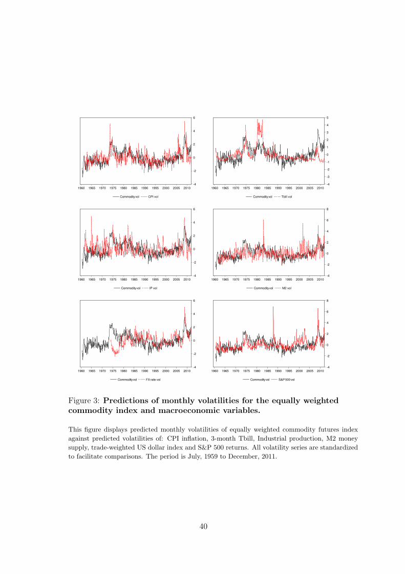
-4

-2

0

2

4

6

1960 1965 1970 1975 1980 1985 1990 1995 2000 2005 2010

Commodity vol CPI vol

-4

-3

-2

-1

0

1

2

3

4

5

1960 1965 1970 1975 1980 1985 1990 1995 2000 2005 2010

Commodity vol Tbill vol

-4

-2

0

2

4

6

1960 1965 1970 1975 1980 1985 1990 1995 2000 2005 2010

Commodity vol IP vol

-4

-2

0

2

4

6

8

1960 1965 1970 1975 1980 1985 1990 1995 2000 2005 2010

Commodity vol M2 vol

-4

-2

0

2

4

6

1960 1965 1970 1975 1980 1985 1990 1995 2000 2005 2010

Commodity vol FX rate vol

-4

-2

0

2

4

6

8

1960 1965 1970 1975 1980 1985 1990 1995 2000 2005 2010

Commodity vol S&P 500 vol

Figure 3: Predictions of monthly volatilities for the equally weightedcommodity index and macroeconomic variables.

This figure displays predicted monthly volatilities of equally weighted commodity futures index

against predicted volatilities of: CPI inflation, 3-month Tbill, Industrial production, M2 money

supply, trade-weighted US dollar index and S&P 500 returns. All volatility series are standardized

to facilitate comparisons. The period is July, 1959 to December, 2011.

40

1.0

1.5

2.0

2.5

3.0

3.5

4.0

1960 1970 1980 1990 2000 2010

Log realized volatility - Equally weighted index

1.0

1.5

2.0

2.5

3.0

3.5

4.0

1960 1970 1980 1990 2000 2010

Log realized volatility - GSCI index

Figure 4: Aggregate commodity volatility during recessions

This figure displays time series plots of the logarithm of realized volatility for the equally weighted

commodity index (upper panel) and the GSCI(Eq) index (lower panel) for the period July 1959 to

December 2011. Superimposed on the graphs are NBER recession months (shaded areas).

41

0.2

0.4

0.6

0.8

1.0

1.2

1990 1995 2000 2005 2010

CPI uncertainty

0.4

0.8

1.2

1.6

2.0

2.4

1990 1995 2000 2005 2010

Industrial production uncertainty

0.0

0.2

0.4

0.6

0.8

1.0

1990 1995 2000 2005 2010

Tbill uncertainty

0

20

40

60

80

100

1990 1995 2000 2005 2010

Net exports uncertainty

Figure 5: Time series plots of dispersion of beliefs

This figure displays the time series plots of short-term dispersion of beliefs of professional forecasters

regarding the following economic series: Tbill, CPI, Industrial Production and Net Exports.

The dispersion series is obtained as the cross-sectional standard deviation across expectations

of individual forecasters over each month. The period under consideration is 1991-2011.

42

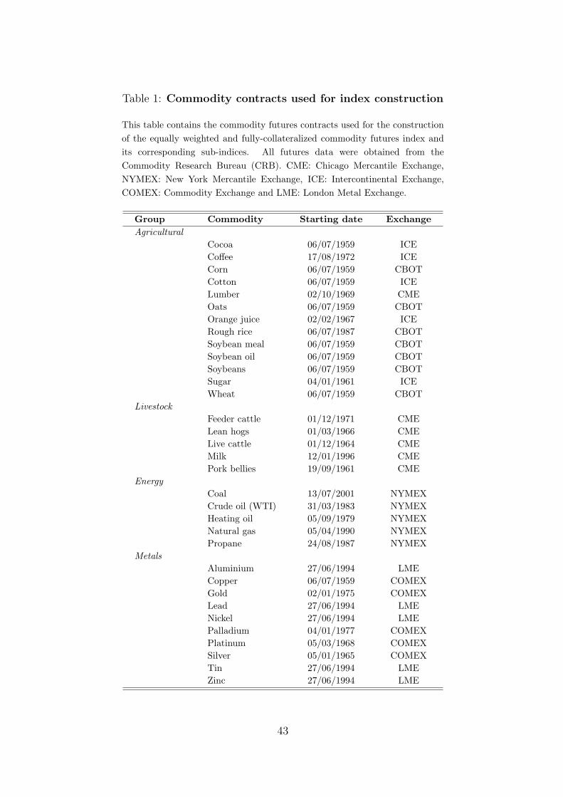
Table 1: Commodity contracts used for index construction

This table contains the commodity futures contracts used for the construction

of the equally weighted and fully-collateralized commodity futures index and

its corresponding sub-indices. All futures data were obtained from the

Commodity Research Bureau (CRB). CME: Chicago Mercantile Exchange,

NYMEX: New York Mercantile Exchange, ICE: Intercontinental Exchange,

COMEX: Commodity Exchange and LME: London Metal Exchange.

Group Commodity Starting date Exchange

Agricultural

Cocoa 06/07/1959 ICE

Coffee 17/08/1972 ICE

Corn 06/07/1959 CBOT

Cotton 06/07/1959 ICE

Lumber 02/10/1969 CME

Oats 06/07/1959 CBOT

Orange juice 02/02/1967 ICE

Rough rice 06/07/1987 CBOT

Soybean meal 06/07/1959 CBOT

Soybean oil 06/07/1959 CBOT

Soybeans 06/07/1959 CBOT

Sugar 04/01/1961 ICE

Wheat 06/07/1959 CBOT

Livestock

Feeder cattle 01/12/1971 CME

Lean hogs 01/03/1966 CME

Live cattle 01/12/1964 CME

Milk 12/01/1996 CME

Pork bellies 19/09/1961 CME

Energy

Coal 13/07/2001 NYMEX

Crude oil (WTI) 31/03/1983 NYMEX

Heating oil 05/09/1979 NYMEX

Natural gas 05/04/1990 NYMEX

Propane 24/08/1987 NYMEX

Metals

Aluminium 27/06/1994 LME

Copper 06/07/1959 COMEX

Gold 02/01/1975 COMEX

Lead 27/06/1994 LME

Nickel 27/06/1994 LME

Palladium 04/01/1977 COMEX

Platinum 05/03/1968 COMEX

Silver 05/01/1965 COMEX

Tin 27/06/1994 LME

Zinc 27/06/1994 LME

43

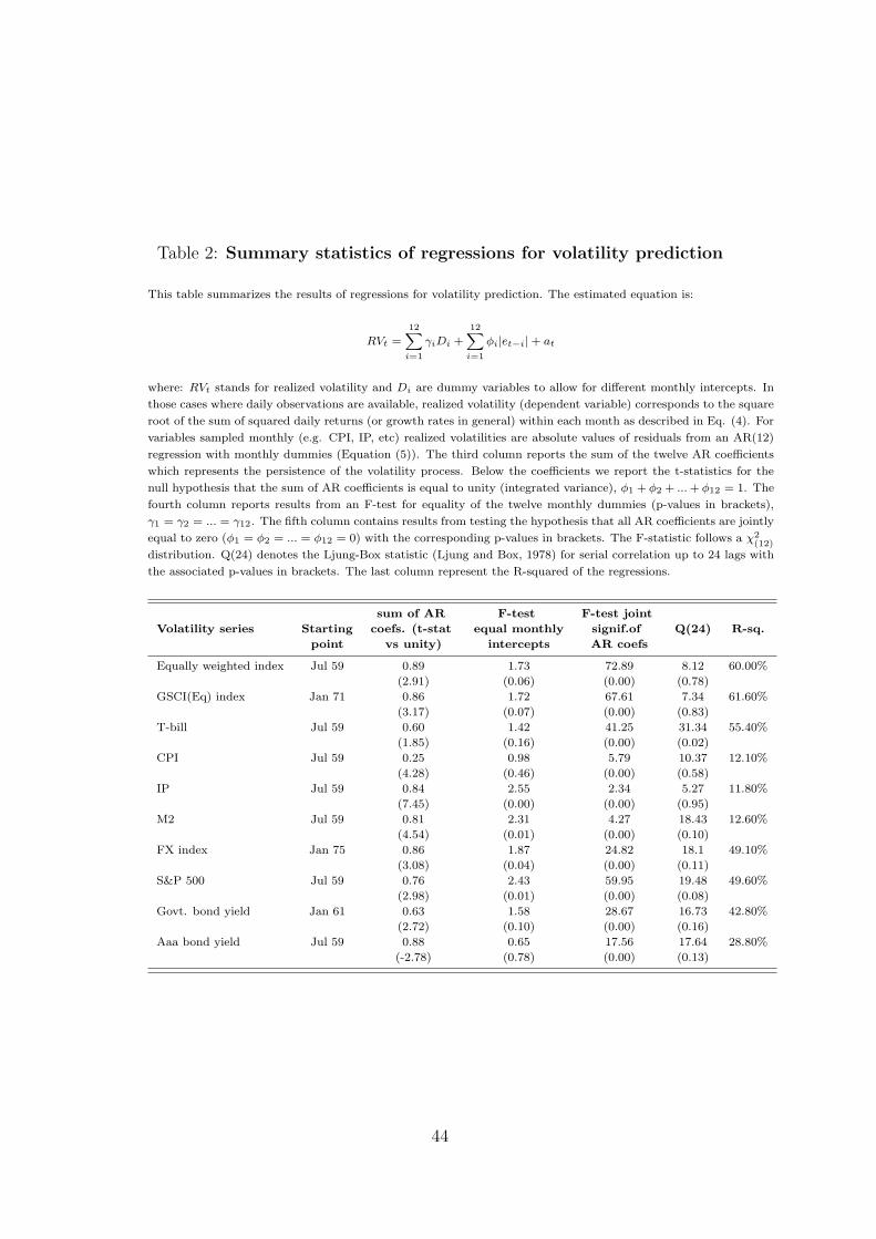
Table 2: Summary statistics of regressions for volatility prediction

This table summarizes the results of regressions for volatility prediction. The estimated equation is:

RVt =12∑i=1

γiDi +12∑i=1

ϕi|et−i|+ at

where: RVt stands for realized volatility and Di are dummy variables to allow for different monthly intercepts. In

those cases where daily observations are available, realized volatility (dependent variable) corresponds to the square

root of the sum of squared daily returns (or growth rates in general) within each month as described in Eq. (4). For

variables sampled monthly (e.g. CPI, IP, etc) realized volatilities are absolute values of residuals from an AR(12)

regression with monthly dummies (Equation (5)). The third column reports the sum of the twelve AR coefficients

which represents the persistence of the volatility process. Below the coefficients we report the t-statistics for the

null hypothesis that the sum of AR coefficients is equal to unity (integrated variance), ϕ1 + ϕ2 + ...+ ϕ12 = 1. The

fourth column reports results from an F-test for equality of the twelve monthly dummies (p-values in brackets),

γ1 = γ2 = ... = γ12. The fifth column contains results from testing the hypothesis that all AR coefficients are jointly

equal to zero (ϕ1 = ϕ2 = ... = ϕ12 = 0) with the corresponding p-values in brackets. The F-statistic follows a χ2(12)

distribution. Q(24) denotes the Ljung-Box statistic (Ljung and Box, 1978) for serial correlation up to 24 lags with

the associated p-values in brackets. The last column represent the R-squared of the regressions.

Volatility series

sum of AR F-test F-test joint

Q(24) R-sq.Starting coefs. (t-stat equal monthly signif.of

point vs unity) intercepts AR coefs

Equally weighted index Jul 59 0.89 1.73 72.89 8.12 60.00%

(2.91) (0.06) (0.00) (0.78)

GSCI(Eq) index Jan 71 0.86 1.72 67.61 7.34 61.60%

(3.17) (0.07) (0.00) (0.83)

T-bill Jul 59 0.60 1.42 41.25 31.34 55.40%

(1.85) (0.16) (0.00) (0.02)

CPI Jul 59 0.25 0.98 5.79 10.37 12.10%

(4.28) (0.46) (0.00) (0.58)

IP Jul 59 0.84 2.55 2.34 5.27 11.80%

(7.45) (0.00) (0.00) (0.95)

M2 Jul 59 0.81 2.31 4.27 18.43 12.60%

(4.54) (0.01) (0.00) (0.10)

FX index Jan 75 0.86 1.87 24.82 18.1 49.10%

(3.08) (0.04) (0.00) (0.11)

S&P 500 Jul 59 0.76 2.43 59.95 19.48 49.60%

(2.98) (0.01) (0.00) (0.08)

Govt. bond yield Jan 61 0.63 1.58 28.67 16.73 42.80%

(2.72) (0.10) (0.00) (0.16)

Aaa bond yield Jul 59 0.88 0.65 17.56 17.64 28.80%

(-2.78) (0.78) (0.00) (0.13)

44

Table 3: Correlations between aggregate commodity return volatilityand macroeconomic volatility

This table reports Spearman’s rank order correlation coefficients between predicted volatility of the equally

weighted commodity futures index and predicted macroeconomic volatilities for the periods: 1970–1990 and

1991-2011.

Series (symbol) cmdvol tbillvol cpivol ipvol m2vol fxvol spvol gvtvol aaavol vix

1970-2011

Eq. weighted index vol (cmdvol) 1.00

–

T-bill vol (tbillvol) 0.31 1.00

(0.00) –

CPI vol (cpivol) 0.49 0.18 1.00

(0.00) (0.00) –

IP vol (ipvol) 0.12 0.17 0.18 1.00

(0.01) (0.00) (0.00) –

M2 vol (m2vol) 0.19 0.04 0.23 0.05 1.00

(0.00) (0.40) (0.00) (0.24) –

FX index vol (fxvol) 0.11 -0.05 0.07 0.05 0.18 1.00

(0.02) (0.33) (0.13) (0.25) (0.00) –

S&P 500 vol (spvol) 0.33 0.16 0.28 0.13 0.15 0.21 1.00

(0.00) (0.00) (0.00) (0.00) (0.00) (0.00) –

Govt. bond yield vol (gvtvol) 0.13 0.34 0.08 0.11 0.19 0.33 0.24 1.00

(0.00) (0.00) (0.09) (0.01) (0.00) (0.00) (0.00) –

Aaa yield vol (aaavol) 0.16 0.21 0.10 0.00 0.16 0.19 0.22 0.61 1.00

(0.00) (0.00) (0.02) (0.93) (0.00) (0.00) (0.00) (0.00) –

1991-2011

Commodity index vol (cmdvol) 1.00

–

Tbill vol (tbillvol) -0.09 1.00

(0.13) –

CPI vol (cpivol) 0.54 0.06 1.00

(0.00) (0.36) –

IP growth vol (ipvol) 0.14 0.14 0.17 1.00

(0.02) (0.03) (0.01) –

M2 vol (m2vol) 0.28 -0.02 0.29 0.03 1.00

(0.00) (0.73) (0.00) (0.62) –

FX index vol (fxvol) 0.46 0.01 0.26 0.22 0.28 1.00

(0.00) (0.93) (0.00) (0.00) (0.00) –

S&P 500 vol (spvol) 0.32 0.26 0.29 0.21 0.23 0.22 1.00

(0.00) (0.00) (0.00) (0.00) (0.00) (0.00) –

Govt. bond yield vol (gvtvol) 0.16 0.15 0.10 0.24 0.34 0.27 0.41 1.00

(0.01) (0.02) (0.10) (0.00) (0.00) (0.00) (0.00) –

Aaa yield vol (aaavol) 0.11 -0.06 0.06 0.02 0.15 -0.05 0.23 0.21 1.00

(0.09) (0.34) (0.34) (0.77) (0.02) (0.41) (0.00) (0.00) –

VIX 0.22 0.10 0.17 0.16 0.17 0.15 0.82 0.29 0.26 1.00

(0.00) (0.11) (0.01) (0.01) (0.02) (0.00) (0.00) (0.00) (0.00) –

45

Table 4: Summary statistics of explanatory variables

This table presents summary statistics for the explanatory variables. The period under consideration is 1970.01 - 2011.12.

The first four central moments are reported for each series along with the autocorrelation coefficients of orders 1 and

12 (denoted ρ1 and ρ12, respectively) and the Ljung-Box Q statistic for autocorrelation up to 24 lags, denoted Q(24).

Also, the table contains Phillips-Perron (1998) unit-root test statistics (Z(t)) with the associated p-values (MacKinnnon,

1994). Realized volatilities of variables sampled at daily frequency are computed as the square root of the sum of squared

daily returns within each month. For the monthly sampled variables we applied the two step algorithm of Schwert (1989)

described by Eq. (5) and (6). All volatility proxies are annualized and expressed as a percentage (multiplied by 100). The

period for most macroeconomic variables is July, 1959 to December, 2011.

Phillips - Perron test

Variable Mean Std. Dev. Skew Kurt. ρ1 ρ12 Q(24) Z(t) prob. Obs.

A. Macroeconomic

T-bill vol 1.08 0.99 2.71 11.51 0.90 0.63 3044.40 -7.27 0.00 492

CPI vol 0.71 0.26 1.59 7.40 0.61 0.30 1165.30 -12.68 0.00 492

IP vol 2.25 0.72 1.46 5.89 0.58 0.01 410.61 -11.35 0.00 492

M2 vol 0.88 0.31 1.59 8.03 0.47 0.30 557.49 -16.03 0.00 492

FX index vol 6.08 1.78 0.60 4.91 0.82 0.42 2286.30 -6.99 0.00 456

B. Financial

S&P 500 vol 14.50 6.06 2.64 14.46 0.79 0.26 1386.70 -7.47 0.00 492

Govt bond yield vol 1.90 0.84 1.78 6.72 0.83 0.59 4343.50 -7.46 0.00 492

Aaa yield vol 0.68 0.35 1.57 5.67 0.86 0.57 4179.60 -5.58 0.00 492

VIX 20.54 7.91 1.53 6.66 0.85 0.38 1127.10 -4.38 0.00 264

Term spread 2.05 1.52 -0.64 3.25 0.95 0.47 3398.30 -3.63 0.00 492

Default spread 1.11 0.47 1.70 6.58 0.96 0.44 3513.00 -3.71 0.00 492

Default return spread -0.02 1.46 -0.46 11.10 -0.04 -0.01 31.04 -23.28 0.00 492

TED spread 0.50 0.48 2.75 12.84 0.87 0.32 566.41 -3.18 0.02 140

46

Table 5: Commodity volatility and the business cycle

This table reports results from regressing realized volatilities of commodity returns and economic

variables on a NBER recession dummy:

RVt = a+6∑

i=1

biRVt−i + γINBER,t + ut (14)

where: INBER,t is an indicator variable that equals one for NBER recession months and zero

otherwise. The last column (∆σ(%)) contains the percentage increase in volatility during

recessions compared to expansions. *, **, *** indicate significance at the 10%, 5% and 1%,

respectively. Newey-West (1987) corrected standard errors were used for the estimations with

12 lags.

Dependent Sample Obs. γ tγ ∆σ(%)

Eq. weight. index vol. 07/1959-12/2011 624 0.11** 2.46 49.11

GSCI(Eq) vol 01/1970-12/2011 461 0.23*** 3.05 47.02

Agricultural vol 07/1959-12/2011 624 0.08 1.52 27.33

Livestock vol 01/1966-12/2011 546 0.06 1.38 23.1

Metals vol 01/1968-12/201 522 0.24*** 2.58 57.38

CPI vol 07/1959-12/2011 612 0.03*** 2.85 72.46

IP vol 07/1959-12/2011 612 0.02** 2.09 42.01

T-bill vol 07/1959-12/2011 624 0.03 0.78 159.95

M2 vol 07/1959-12/2011 612 0.03** 2.49 57.56

FX rate vol 01/1975-12/2011 462 0.05 1.45 22.92

S&P 500 vol 07/1959-12/2013 624 0.20** 2.17 58.09

Govt. bond vol 01/1963-12/2011 594 0.04** 2.15 70.73

Aaa yield vol 07/1959-12/2011 612 0.01 1.64 69.15

47

Tab

le6:

Predictiveregressionsforvolatility

ofth

eequallyweightedco

mmodityindex

Thistable

presents

resu

ltsfrom

in-sample

regressionsoflogrealizedvolatility

ofth

eeq

uallyweightedco

mmodityfutu

resindex

onvariousmacroeconomic,

financialandco

mmodity-specificvariables.

Theestimatedmodel

is:

RV

t=

a+

γX

i,t−

1+

6 ∑ j=1

b jRV

t−j+

e t

whereRV

tis

thelogarith

mofrealizedvolatility

(computedbyEquation(4))

ofaneq

uallyweightedindex

ofallmajorco

mmoditiestraded

inth

eUS

market,X

i,t−

1is

thescalarvalueofpredictoriin

month

t−

1obtained

byEq.(6)forvolatility

variables.

Weinclude6lagsonth

erightsideofth

e

equationto

accountforth

epersisten

ceofth

erealizedvolatility

process.Theeq

uationsreferto

one-by-oneestimationsagainst

each

variable.Columns

(2)to

(4)co

ntain

theresu

ltsforth

efullsample

periodsp

anning1970.01to

2011.12.Theremainingco

lumnsofth

etable

report

estimationresu

ltsfor

sub-samplesofth

een

tire

sample

period.

All

variablesare

standard

ized

priorto

theestimationsusingth

esample

mea

nand

standard

dev

iation.

We

report

forea

chforeca

stingvariable

theestimatedco

efficien

t(γ

)forea

chex

planatory

variable

alongwithth

ech

angein

theadjusted

R-square

(den

oted

∆R

2)relativeto

anAR(6)sp

ecifica

tionth

atserves

asaben

chmark.New

ey-W

est(1987)co

rrectedstandard

errors

wereem

ployed

forth

eestimations

(with12lags).*,**,and***indicate

significa

nce

atth

e10%,5%

and10%

level,resp

ectively.

Entire

sample

Sub-sample

1Sub-sample

2Sub-sample

3

1970-2011

1970-1990

1991-2011

2001-2011

Variable

γt γ

∆R

2γ

t γ∆R

2γ

t γ∆R

2γ

t γ∆R

2

S&P

500vol

0.04

1.17

0.02

0.01

0.28

-0.21

0.08*

1.85

0.27

0.04

0.57

-0.26

T-billvol

0.03

1.45

0.00

0.04

0.88

-0.11

0.06

0.81

0.12

0.11

1.38

0.86

Govtbondyield

vol

0.00

0.17

-0.09

-0.03

-0.62

-0.14

0.09**

2.05

0.49

0.03

0.59

-0.29

Aaayield

vol

-0.01

-0.20

-0.09

-0.01

-0.17

-0.21

0.00

-0.02

-0.18

-0.03

-0.36

-0.28

FX

index

vol

--

--

--

0.02

0.45

-0.16

0.03

0.41

-0.32

CPIvol

0.15***

4.30

1.50

0.17***

3.12

1.96

0.14***

3.15

0.97

0.08*

1.88

0.10

IPvol

0.01

0.25

-0.09

-0.05

-1.12

0.03

0.05

1.20

0.05

0.07

1.04

-0.02

M2vol

0.03

1.16

-0.02

0.01

0.16

-0.22

0.06*

1.78

0.14

0.03

0.67

-0.27

Term

spread

-0.02

-0.87

-0.04

-0.07*

-1.95

0.20

0.03

0.87

-0.11

0.02

0.47

-0.31

Default

spr.

0.02

0.48

-0.07

-0.03

-0.53

-0.14

0.04

0.84

-0.09

-0.01

-0.09

-0.37

Default

retu

rnsp

r.-0.05**

-1.99

0.24

-0.07**

-2.00

0.33

-0.06

-1.29

0.21

-0.12**

-2.05

0.99

TED

spread

--

--

--

0.07

1.34

0.30

0.17***

2.84

1.93

VIX

--

--

--

0.13**

2.39

1.17

0.17**

1.99

2.11

IPgrowth

0.00

-0.08

-0.09

0.05

1.20

0.00

-0.10*

-1.85

0.64

-0.13*

-1.84

1.05

OI

--

--

--

0.09**

2.50

0.63

0.10**

2.01

0.53

HP

(hed

gers)

--

--

--

0.09***

2.59

0.70

0.07**

2.05

0.14

HP

(specul.)

--

--

--

0.05

1.35

0.06

0.09**

2.29

0.36

Basis

-0.05

-0.86

-0.01

0.04

0.54

-0.14

-0.23***

-3.13

0.90

-0.26***

-3.25

1.38

48

Tab

le7:

Predictiveregressionsforth

erealize

dvolatility

ofagricu

ltura

lsu

b-index

This

table

reportsresu

ltsfrom

regressionsofrealizedretu

rnvolatility

ofaneq

uallyweightedindex

ofagricu

lturalco

mmoditiesonvariousmacroeconomic,

financialandco

mmodity-specificvariables.

Theestimatedregressionis

given

byEq.(8).

Rea

lizedco

mmodityvolatility

ofea

chmonth

isco

mputedas

thesquare

rootofth

esu

mofsquareddailyretu

rnswithin

each

month

.Thelogarith

mofco

mmodityretu

rnvolatility

isco

nsidered

forth

eestimations.

Weinclude6lagson

therightsideofth

eeq

uation

tomodel

thepersisten

ceofth

erealized

volatility

process.This

number

oflagsis

alsosu

fficien

tto

elim

inate

theautoco

rrelationin

regressionresiduals.Theeq

uationsreferto

one-by-oneestimationsagainst

each

variable.Theestimationsare

perform

ed

on

thefull

sample

period

(1970.01to

2011.12)aswellason

varioussu

b-samples.

All

variablesare

standard

ized

before

theestimations.

Wereport

for

each

explanatory

variable

theestimatedco

efficien

t(γ

)together

withitst-statistic

andth

ech

angein

theadjusted

R-square

(∆R

2)relativeto

anAR(6)

specifica

tionth

atserves

asaben

chmark.New

ey-W

est(1987)co

rrectedstandard

errors

wereem

ployed

forth

eestimations(w

ith12lags).*,**,and***

indicate

significa

nce

atth

e10%,5%

and10%

level,resp

ectively.

Entire

sample

Sub-sample

1Sub-sample

2Sub-sample

3

1970-2011

1970-1990

1991-2011

2001-2011

Variable

γt γ

∆R

2γ

t γ∆R

2γ

t γ∆R

2γ

t γ∆R

2

S&P

500vol

0.07**

2.26

0.32

0.01

0.21

-0.23

0.13***

3.13

1.05

0.09*

1.78

0.28

T-billvol

0.01

0.35

-0.11

0.01

0.30

-0.23

0.02

0.22

-0.21

0.06

0.67

-0.04

Govtbondyield

vol

-0.02

-0.80

-0.07

-0.06

-1.58

0.17

0.10**

2.18

0.74

0.06

1.03

-0.16

Aaayield

vol

-0.01

-0.30

-0.11

-0.03

-0.66

-0.16

0.04

0.92

-0.11

0.04

0.48

-0.30

FX

index

vol

--

--

--

0.12**

2.30

0.78

0.15

1.63

0.71

CPIvol

0.18***

4.93

2.53

0.16***

3.58

2.13

0.21***

3.16

2.75

0.08

1.13

0.12

IPvol

0.01

0.29

-0.11

-0.02

-0.45

-0.19

0.05

1.05

-0.04

0.04

0.55

-0.32

M2vol

0.08***

2.83

0.51

0.03

0.82

-0.13

0.12***

2.96

1.12

0.08

1.27

0.14

Term

spread

0.01

0.37

-0.11

-0.04

-1.16

-0.11

0.06**

2.00

0.16

0.05

1.19

-0.24

Default

spr.

0.03

0.82

-0.05

-0.04

-0.93

-0.08

0.15**

2.50

1.07

0.08

1.10

-0.06

Default

retu

rnsp

r.-0.04

-1.36

0.09

-0.04

-1.01

-0.04

-0.06

-1.11

0.10

-0.14**

-2.04

1.59

TED

spread

--

--

--

0.05

0.82

-0.04

0.13**

2.11

1.05

VIX

--

--

--

0.10*

1.87

0.59

0.13*

1.82

1.19

IPgrowth

0.00

0.08

-0.12

0.05

1.17

0.04

-0.08

-1.27

0.34

-0.12

-1.36

0.89

OI

--

--

--

0.02

0.42

-0.21

0.00

0.00

-0.45

HP

(hed

gers)

--

--

--

0.05

1.21

0.03

0.10

1.63

0.59

HP

(specul.)

--

--

--

0.05

1.07

-0.04

0.12**

2.04

0.72

Basis

-0.06*

-1.76

0.42

-0.12***

-2.81

1.51

-0.15***

-2.58

0.85

0.05

0.98

-0.16

49

Tab

le8:

Predictiveregressionsforth

erealize

dvolatility

oflivestock

sub-index

This

table

reportsresu

ltsfrom

in-sample

regressionsofrealized

retu

rnvolatility

ofan

equally

weighted

index

ofanim

alco

mmoditieson

various

macroeconomic,financialandco

mmodity-specificvariables.

Theestimatedregressionis

given

byEq.(8).

Rea

lizedco

mmodityvolatility

ofea

chmonth

is

computedasth

esquare

rootofth

esu

mofsquareddailyretu

rnswithin

each

month

.Thelogarith

mofco

mmodityretu

rnvolatility

isco

nsidered

forth

e

estimations.

Weinclude6lagsonth

erightsideofth

eeq

uationto

model

thepersisten

ceofth

erealizedvolatility

process.Expost,th

isnumber

oflags

proves

toelim

inatesth

eautoco

rrelationin

regressionresiduals.Theeq

uationsreferto

one-by-oneestimationsagainst

each

variable.Theestimationsare

perform

edonth

efullsample

period(1970.01to

2011.12)aswellasonvarioussu

b-samples.

Allvariablesare

standard

ized

before

theestimations.

We

report

forea

chex

planatory

variable

theestimatedco

efficien

t(γ

)together

withitst-statistic

andth

ech

angein

theadjusted

R-square

(∆R

2)relativeto

anAR(6)sp

ecifica

tionth

atserves

asaben

chmark.New

ey-W

est(1987)co

rrectedstandard

errors

wereem

ployed

forth

eestimations(w

ith12lags).*,**,

and***indicate

significa

nce

atth

e10%,5%

and10%

level,resp

ectively.

Entire

sample

Sub-sample

1Sub-sample

2Sub-sample

3

1970-2011

1970-1990

1991-2011

2001-2011

Variable

γt γ

∆R

2γ

t γ∆R

2γ

t γ∆R

2γ

t γ∆R

2

S&P

500vol

0.04*

1.76

0.06

0.04

1.51

-0.04

0.10**

2.48

0.69

0.12

1.46

0.87

T-billvol

0.06***

2.59

0.18

0.03

1.09

-0.11

0.02

0.36

-0.26

0.04

0.42

-0.54

Govtbondyield

vol

0.02

0.74

-0.06

0.00

-0.07

-0.19

0.09*

1.66

0.41

0.14*

1.83

1.37

Aaayield

vol

0.00

-0.02

-0.10

-0.01

-0.32

-0.18

0.00

-0.01

-0.29

0.04

0.86

-0.50

FX

index

vol

--

--

--

0.10**

2.34

0.57

0.16*

1.95

1.34

CPIvol

0.09***

2.91

0.72

0.14***

4.05

1.49

0.07

1.42

0.23

0.05

0.60

-0.39

IPvol

0.00

0.12

-0.10

-0.07

-1.63

0.26

0.10***

2.68

0.77

0.17***

3.01

2.47

M2vol

0.01

0.38

-0.09

0.01

0.37

-0.18

0.04

0.50

-0.16

0.11

1.20

0.65

Term

spread

-0.05

-1.61

0.16

-0.07*

-1.83

0.36

0.02

0.33

-0.25

0.18**

1.99

1.81

Default

spr.

0.03

0.81

-0.04

-0.02

-0.46

-0.15

0.07*

1.82

0.21

0.12**

2.10

0.83

Default

retu

rnsp

r.-0.02

-0.47

-0.08

0.04

0.73

-0.05

-0.07

-1.47

0.20

-0.16**

-2.20

2.12

TED

spread

--

--

--

0.04

0.76

-0.15

0.04

0.48

-0.52

VIX

--

--

--

0.14***

2.71

1.51

0.16*

1.94

2.33

IPgrowth

-0.07**

-2.06

0.32

0.00

0.10

-0.19

-0.18***

-4.03

2.98

-0.17*

-1.74

2.78

OI

--

--

--

-0.04

-0.71

-0.13

-0.06

-0.68

-0.30

HP

(hed

gers)

--

--

--

-0.14***

-2.58

1.63

-0.04

-0.53

-0.47

HP

(specul.)

--

--

--

-0.17***

-2.97

2.50

-0.16*

-1.81

2.19

Basis

0.00

0.09

-0.10

0.04

0.76

-0.06

-0.02

-0.31

-0.25

-0.17**

-2.04

2.83

50

Tab

le9:

Predictiveregressionsforth

erealize

dvolatility

ofenerg

ysu

b-index

This

table

reportsresu

ltsfrom

in-sample

regressionsofrealized

retu

rnvolatility

ofan

equally

weighted

portfolio

ofen

ergy

commoditieson

various

macroeconomic,financialand

commodity-specificvariables.

Resultsare

notreported

forth

efirsttw

osample

periodsbecause

pricesformost

energy

commoditiesbecomeavailable

after

’80s,

timeth

atco

rrespondsto

theirdate

ofinclusionin

theindex

(see

table

1).

Rea

lizedco

mmodityvolatility

ofea

ch

month

isco

mputedasth

esquare

rootofth

esu

mofsquareddailyretu

rnswithin

each

month

.Thelogarith

mofco

mmodityretu

rnvolatility

isco

nsidered

forth

eestimations.

Weinclude6lagsonth

erightsideofth

eeq

uationto

model

thepersisten

ceofth

erealizedvolatility

process.Ex-post

this

number

oflagsis

adeq

uate

toelim

inate

theautoco

rrelation

inregression

residuals.

Theeq

uationsreferto

one-by-oneestimationsagainst

each

variable.

The

estimationsare

perform

edon

thefull

sample

period

(1970.01to

2011.12)aswellason

varioussu

b-samples.

All

variablesare

standard

ized

before

the

estimations.

Wereport

forea

chex

planatory

variable

theestimatedco

efficien

t(γ

)together

withitst-statistic

andth

ech

angein

theadjusted

R-square

(∆R

2)relativeto

anAR(6)sp

ecifica

tionth

atserves

asaben

chmark.New

ey-W

est(1987)co

rrectedstandard

errors

wereem

ployed

forth

eestimations

(with12lags).*,**,and***indicate

significa

nce

atth

e10%,5%

and10%

level,resp

ectively.

Entire

sample

Sub-sample

1Sub-sample

2Sub-sample

3

1970-2011

1970-1990

1991-2011

2001-2011

Variable

γt γ

∆R

2γ

t γ∆R

2γ

t γ∆R

2γ

t γ∆R

2

S&P

500vol

--

--

--

0.10*

1.87

0.58

0.10

1.34

0.40

T-billvol

--

--

--

0.09*

1.74

0.75

0.20**

2.13

3.32

Govtbondyield

vol

--

--

--

0.05

1.17

0.05

0.11***

2.79

0.51

Aaayield

vol

--

--

--

0.01

0.23

-0.22

0.01

0.26

-0.52

FX

index

vol

--

--

--

-0.01

-0.25

-0.21

0.00

0.03

-0.53

CPIvol

--

--

--

0.07

0.96

0.12

0.05

0.56

-0.35

IPvol

--

--

--

0.06

1.23

0.17

0.09

1.08

0.21

M2vol

--

--

--

0.06

1.08

0.07

0.06

0.80

-0.18

Term

spread

--

--

--

-0.04

-1.07

-0.03

0.04

0.71

-0.38

Default

spr.

--

--

--

0.07

1.39

0.11

0.09

1.22

-0.02

Default

retu

rnsp

r.-

--

--

--0.10***

-2.98

0.82

-0.15***

-2.84

1.44

TED

spread

--

--

--

0.08

1.35

0.38

0.16*

1.89

1.78

VIX

--

--

--

0.18***

3.10

2.77

0.17**

2.05

2.15

IPgrowth

--

--

--

-0.06

-1.45

0.15

-0.12*

-1.95

0.71

OI

--

--

--

0.06*

1.71

0.13

0.05

0.74

-0.38

HP

(hed

gers)

--

--

--

0.02

0.44

-0.18

0.02

0.22

-0.51

HP

(specul.)

--

--

--

0.00

0.10

-0.22

0.02

0.32

-0.51

Basis

--

--

--

-0.16***

-2.67

2.07

-0.04

-0.62

-0.29

51

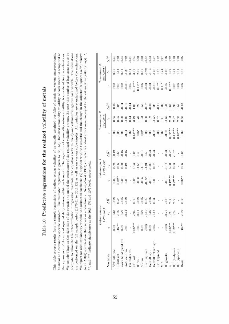
Tab

le10:Predictiveregressionsforth

erealize

dvolatility

ofmetals

This

table

reportsresu

ltsfrom

in-sample

regressionsofrealizedretu

rnvolatility

ofaneq

uallyweightedportfolioofmetals

onvariousmacroeconomic,

financialandco

mmodity-specificvariables.

Theestimatedregressionis

given

byEq.(8).

Rea

lizedco

mmodityvolatility

ofea

chmonth

isco

mputedas

thesquare

rootofth

esu

mofsquareddailyretu

rnswithin

each

month

.Thelogarith

mofco

mmodityretu

rnvolatility

isco

nsidered

forth

eestimations.

Weinclude6lagsonth

erightsideofth

eeq

uationto

model

thepersisten

ceofth

erealizedvolatility

process.Ex-post

this

number

oflagstu

rnsoutto

be

adeq

uate

toelim

inate

theautoco

rrelationin

regressionresiduals.Theeq

uationsreferto

one-by-oneestimationsagainst

each

variable.Theestimations

are

perform

edonth

efullsample

period(1970.01to

2011.12)aswellasonvarioussu

b-samples.

Allvariablesare

standard

ized

before

theestimations.

Wereport

forea

chex

planatory

variable

theestimatedco

efficien

t(γ

)together

withitst-statistic

andth

ech

angein

theadjusted

R-square

(∆R

2)relative

toanAR(6)sp

ecifica

tionth

atserves

asaben

chmark.New

ey-W

est(1987)co

rrectedstandard

errors

wereem

ployed

forth

eestimations(w

ith12lags).*,

**,and***indicate

significa

nce

atth

e10%,5%

and10%

level,resp

ectively.

Entire

sample

Sub-sample

1Sub-sample

2Sub-sample

3

1970-2011

1970-1990

1991-2011

2001-2011

Variable

γt γ

∆R

2γ

t γ∆R

2γ

t γ∆R

2γ

t γ∆R

2

S&P

500vol

0.01

0.32

-0.08

0.02

0.59

-0.19

0.03

0.65

-0.10

0.02

0.37

-0.30

T-billvol

0.07**

2.16

0.23

0.12**

2.06

0.63

0.05

0.95

0.08

0.07

1.14

0.20

Govtbondyield

vol

0.02

0.58

-0.05

0.03

0.50

-0.16

0.04

0.90

-0.04

0.02

0.31

-0.32

Aaayield

vol

-0.01

-0.24

-0.08

0.03

0.49

-0.16

-0.04

-1.01

-0.01

-0.08

-1.31

0.22

FX

index

vol

--

--

--

0.02

0.44

-0.14

0.04

0.91

-0.20

CPIvol

0.08***

2.94

0.39

0.06

1.23

0.05

0.13***

3.49

1.00

0.11***

3.07

0.74

IPvol

-0.01

-0.21

-0.08

-0.08

-1.56

0.40

0.06*

1.76

0.22

0.11**

2.45

0.80

M2vol

0.02

0.68

-0.05

-0.05

-1.10

-0.01

0.09*

1.93

0.59

0.06

0.97

0.00

Term

spread

-0.03

-1.15

0.02

-0.09*

-1.91

0.50

0.03

0.80

-0.07

-0.01

-0.22

-0.33

Default

spr.

0.02

0.46

-0.06

-0.01

-0.09

-0.23

0.03

1.02

-0.10

-0.01

-0.14

-0.34

Default

retu

rnsp

r.-0.04

-1.13

0.04

0.00

0.07

-0.23

-0.08

-1.58

0.39

-0.10

-1.61

0.67

TED

spread

--

--

--

0.03

0.57

-0.11

0.07*

1.68

0.12

VIX

--

--

--

0.07

1.41

0.32

0.11*

1.74

0.97

IPgrowth

-0.03

-0.79

-0.01

-0.01

-0.14

-0.23

-0.08

-1.64

0.41

-0.07

-1.01

0.16

OI

0.08***

3.21

2.00

0.12***

3.50

-0.77

0.09***

2.83

0.66

0.07**

1.99

0.22

HP

(hed

gers)

0.12***

3.74

2.50

0.22***

2.83

-1.57

0.11***

2.97

0.90

0.07

1.21

0.10

HP

(specul.)

--

--

--

0.10***

2.58

0.52

0.08

1.31

0.10

Basis

0.04**

2.18

0.06

0.06**

2.06

0.05

0.02

0.56

-0.13

0.06

1.38

0.05

52

Tab

le11:Predictiveregressionsforth

evolatility

ofth

eGSCIindex

This

table

presents

resu

ltsfrom

regressionsofth

elogarith

mofrealized

retu

rnvolatility

ofth

eGoldman

Sach

sCommodity

Index

(GSCI)

against

macroeconomic

financialandco

mmodity-specificvariables.

Theresu

ltsco

rrespondto

univariate

regressionsagainst

each

individualpredictor.

Instea

dof

usingth

eretu

rnsofth

estandard

GSCIindex

which

isdominated

byen

ergyco

mmodities,

weco

nsider

an

equally-w

eighted

variantofit

bytakingth

e

averagedailyretu

rnacross

allitssu

b-indices

comprisedofagricu

ltural,livestock

,en

ergyco

mmoditiesandmetals.Theestimationsare

perform

edforth

e

fullsample

period1970.01-2011.12aswellasforvarioussu

b-periods.

Allvariablesare

standard

ized

before

theestimation.W

ereport

forea

chex

planatory

variable

theestimatedco

efficien

t(γ

)together

withitst-statistic

andth

ech

angein

theadjusted

R-square

(∆R

2)relativeto

anAR(6)sp

ecifica

tionth

at

serves

asaben

chmark.New

ey-W

est(1987)co

rrectedstandard

errors

wereem

ployed

forth

eestimations(w

ith12lags).*,**,and***indicate

significa

nce

atth

e10%,5%

and10%

level,resp

ectively.

Entire

sample

Sub-sample

1Sub-sample

2Sub-sample

3

1970-2011

1970-1990

1991-2011

2001-2011

Variable

γt γ

∆R

2γ

t γ∆R

2γ

t γ∆R

2γ

t γ∆R

2

S&P

500vol

0.04

1.34

0.04

0.04

1.27

-0.03

0.07

1.63

0.18

0.08

0.97

0.05

T-billvol

0.03

1.03

-0.02

0.02

0.34

-0.18

0.03

0.55

-0.05

0.10

1.19

0.58

Govtbondyield

vol

-0.01

-0.41

-0.07

-0.05

-1.26

0.06

0.06

1.34

0.15

0.03

0.51

-0.36

Aaayield

vol

-0.02

-0.82

-0.03

-0.03

-0.79

-0.08

-0.02

-0.48

-0.13

-0.04

-0.53

-0.30

FX

index

vol

--

--

--

-0.01

-0.21

-0.16

0.03

0.37

-0.41

CPIvol

0.13***

3.99

1.02

0.14***

2.80

1.42

0.13***

2.95

0.91

0.13*

1.97

0.79

IPvol

0.00

-0.11

-0.08

-0.06

-1.20

0.12

0.04

0.84

-0.04

0.10

1.27

0.46

M2vol

0.01

0.49

-0.07

-0.02

-0.59

-0.15

0.05

1.62

0.09

0.04

0.90

-0.29

Term

spread

-0.05**

-2.06

0.18

-0.09**

-2.28

0.59

-0.01

-0.41

-0.15

-0.01

-0.12

-0.44

Default

spr.

0.00

-0.04

-0.08

-0.05

-0.89

0.02

0.02

0.64

-0.14

0.02

0.24

-0.43

Default

retu

rnsp

r.-0.06**

-2.39

0.30

-0.07*

-1.79

0.25

-0.07*

-1.82

0.39

-0.15***

-2.65

1.83

TED

spread

--

--

--

0.05

0.91

0.03

0.18***

2.59

2.00

VIX

--

--

--

0.14***

3.09

1.55

0.19**

2.31

3.03

IPgrowth

-0.01

-0.20

-0.08

0.04

1.24

-0.01

-0.08*

-1.85

0.47

-0.13*

-1.93

1.27

OI

0.09***

3.70

1.41

0.08**

2.02

1.94

0.10***

2.64

0.84

0.10*

1.91

0.51

HP

(hed

gers)

0.09***

3.25

0.77

0.11***

3.01

1.36

0.09**

2.37

0.66

0.08**

2.02

0.14

HP

(specul.)

--

--

--

0.05

1.25

0.12

0.10**

2.24

0.54

Basis

-0.02

-0.40

-0.07

0.05

0.78

-0.08

-0.13*

-1.76

0.22

-0.19**

-1.98

0.54

53

Table 12: Estimates of the relationship between commodity returnvolatility and macroeconomic variables

This table reports results from regressions where the logarithm of realized commodity return volatility is regressed

on lagged macroeconomic volatility proxies. Columns (2) and (7) report estimation results for the volatilities

of the equally-weighted commodity index and GSCI index, respectively. Columns (3) to (6) display results

for the realized volatilities of the equally-weighted sectoral commodity indices. The estimations are performed

for the full sample period 1970.01 - 2011.12 and over three sub-samples: 1970.01-1990.12, 1991.01-2011.12 and

2001.01-2011.12. The row denoted ∆R2 contains the percentage change in the adjusted R2 of an AR(6) model

after including the macroeconomic volatility proxies. The Newey-West corrected t-statistics (with 12 lags) are

reported in brackets below each coefficient. *, **, and *** indicate significance at the 10%, 5% and 1% level,

respectively.

Variable Eq. weighted Agricultural Livestock Energy Metals GSCI(Eq)

1970-2011

T-bill vol 0.04* -0.01 0.05** - 0.08** 0.04

(1.89) (-0.38) (2.31) - (2.45) (1.48)

CPI vol 0.16*** 0.18*** 0.10*** - 0.09*** 0.14***

(4.38) (4.61) (3.15) - (2.95) (4.06)

IP vol -0.02 -0.03 -0.02 - -0.03 -0.03

(-0.78) (-0.89) (-0.79) - (-1.00) (-1.05)

M2 vol 0.01 0.05 -0.01 - 0.01 -0.01

(0.34) (1.46) (-0.35) - (0.27) (-0.20)

∆R2 1.40 2.50 0.70 0.60 0.90

1970-1990

T-bill vol 0.04 -0.02 0.02 - 0.14** 0.03

(1.13) (-0.59) (0.59) - (2.41) (0.57)

CPI vol 0.18*** 0.17*** 0.15*** - 0.07 0.16***

(3.25) (3.42) (4.62) - (1.60) (3.02)

IP vol -0.07 -0.04 -0.08* - -0.10** -0.07

(-1.65) (-0.83) (-1.88) - (-1.99) (-1.52)

M2 vol -0.02 0.01 -0.01 - -0.05 -0.04

(-0.49) (0.17) (-0.19) - (-1.04) (-1.08)

∆R2 1.90 1.70 1.50 1.50 1.50

1991-2011

T-bill vol 0.04 -0.03 -0.01 0.09* 0.02 0.02

(0.57) (-0.32) (-0.27) (1.91) (0.47) (0.33)

CPI vol 0.13** 0.18*** 0.02 0.14** 0.10** 0.13**

(2.53) (2.84) (0.32) (1.99) (2.06) (2.54)

IP vol 0.02 -0.00 0.08* 0.04 0.03 0.01

(0.42) (-0.02) (1.73) (0.69) (0.86) (0.21)

M2 vol 0.04 0.08* -0.00 0.03 0.07 0.04

(0.98) (1.85) (-0.00) (0.48) (1.33) (1.04)

FX index vol -0.01 0.05 0.06 -0.05 -0.04 -0.05

(-0.12) (0.79) (0.91) (-0.90) (-0.77) (-0.97)

∆R2 0.70 2.70 0.00 2.00 1.00 0.50

2001-2011

T-bill vol 0.10 0.04 -0.03 0.20** 0.04 0.08

(1.31) (0.44) (-0.37) (2.33) (0.73) (0.90)

CPI vol 0.05 0.05 -0.07 0.08 0.07 0.09

(0.85) (0.68) (-0.82) (0.81) (1.25) (1.31)

IP vol 0.03 -0.01 0.17** 0.06 0.08 0.06

(0.47) (-0.20) (2.03) (0.57) (1.39) (0.70)

M2 vol 0.01 0.04 0.07 0.05 0.04 0.03

(0.25) (0.58) (0.73) (0.58) (0.62) (0.51)

FX index vol 0.03 0.12 0.09 0.04 -0.03 -0.01

(0.29) (1.08) (0.84) (0.39) (-0.38) (-0.11)

∆R2 -0.10 -0.50 1.10 3.30 0.30 0.10

54

Table 13: Estimates of regressions between commodity returnvolatility and financial/commodity-specific variables

This table reports results from regressions where the logarithm of realized commodity return volatility is regressed

on lagged financial and commodity specific variables. The row denoted ∆R2 contains the percentage change in the

adjusted R2 of an AR(6) model after including the macroeconomic volatility proxies. The Newey-West corrected

t-statistics (with 12 lags) are reported in brackets below each coefficient. *, **, and *** indicate significance at

the 10%, 5% and 1% level, respectively.

Variable Eq. weighted Agricultural Livestock Energy Metals GSCI(Eq)

1970-2011

S&P 500 vol 0.04 0.09** 0.06** - 0.02 0.05*

(1.49) (2.54) (2.15) - (0.58) (1.94)

Aaa vol -0.01 0.00 -0.01 - -0.02 -0.03

(-0.22) (0.03) (-0.28) - (-0.44) (-0.91)

Term spread -0.03 0.02 -0.06* - -0.02 -0.06**

(-0.99) (0.55) (-1.70) - (-0.74) (-2.34)

Default return -0.06** -0.04 -0.00 - -0.03 -0.05**

(-2.04) (-1.34) (-0.13) - (-1.02) (-2.10)

Basis -0.04 -0.10** -0.05 - 0.05 -0.03

(-0.92) (-2.44) (-1.64) - (1.48) (-0.70)

∆R2 0.00 1.00 0.30 - 0.00 0.40

1970-1990

S&P 500 vol 0.01 0.02 0.04 - 0.03 0.07*

(0.16) (0.47) (1.45) - (1.04) (1.97)

Aaa vol 0.02 0.03 -0.02 - 0.04 -0.04

(0.57) (0.63) (-0.42) - (0.69) (-0.77)

Term spread -0.05 -0.02 -0.09* - -0.09* -0.10**

(-1.35) (-0.59) (-1.92) - (-1.68) (-2.38)

Default return -0.09* -0.03 0.05 - 0.02 -0.06**

(-2.45) (-0.78) (0.87) - (0.37) (-2.25)

Basis -0.03 -0.14*** -0.04 - 0.07 -0.03

(-0.46) (-2.89) (-0.74) - (1.30) (-0.48)

∆R2 -0.10 0.60 0.50 - 0.20 0.70

1991-2011

VIX 0.18** 0.10* 0.13** 0.26*** 0.11** 0.21***

(2.56) (1.70) (2.30) (4.03) (1.99) (3.75)

Aaa vol -0.05 0.02 -0.03 -0.04 -0.05 -0.08**

(-1.08) (0.46) (-0.33) (-0.74) (-1.26) (-2.01)

Term spread -0.03 0.05 0.06 -0.06 0.00 -0.09***

(-0.90) (1.20) (0.98) (-1.35) (0.00) (-2.66)

Default return -0.03 -0.05 -0.04 -0.02 -0.06 -0.03

(-0.71) (-1.04) (-0.98) (-0.61) (-1.41) (-0.86)

Basis -0.02 -0.03 -0.15*** -0.16*** -0.03 0.01

(-0.44) (-0.62) (-3.19) (-4.13) (-0.78) (0.15)

HP (hedg.) 0.13** 0.05 -0.06 0.01 0.13*** 0.16***

(2.59) (1.03) (-1.08) (0.29) (2.60) (3.46)

∆R2 1.80 0.41 2.60 6.20 1.70 2.90

2001-2011

VIX 0.22** 0.08 0.10 0.22** 0.23*** 0.26***

(2.16) (0.90) (0.89) (2.51) (3.79) (3.10)

AAA vol -0.06 0.05 -0.01 -0.05 -0.11* -0.07

(-0.72) (0.64) (-0.08) (-0.80) (-1.96) (-1.05)

Term spread -0.09 0.02 0.23** 0.00 -0.09 -0.14**

(-1.61) (0.53) (2.29) (0.03) (-1.48) (-2.43)

Default return -0.05 -0.13** -0.14** -0.06 -0.02 -0.06

(-1.13) (-2.14) (-2.11) (-1.43) (-0.43) (-1.64)

Basis -0.11* 0.01 -0.14* -0.09** -0.00 -0.08

(-1.95) (0.15) (-1.87) (-2.12) (-0.06) (-1.29)

HP (hedg.) 0.11 0.10* -0.14* 0.03 0.17** 0.15**

(1.47) (1.67) (-1.87) (0.55) (2.14) (2.01)

∆R2 3.50 1.63 6.10 2.70 3.10 5.20

55

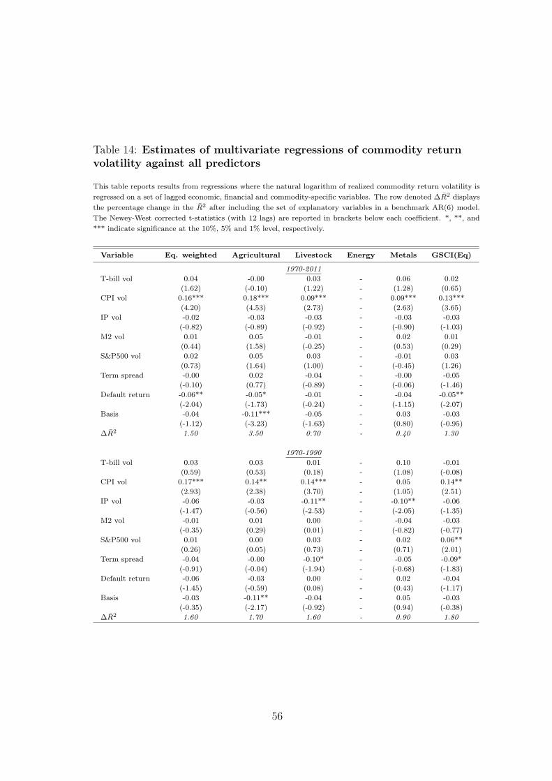
Table 14: Estimates of multivariate regressions of commodity returnvolatility against all predictors

This table reports results from regressions where the natural logarithm of realized commodity return volatility is

regressed on a set of lagged economic, financial and commodity-specific variables. The row denoted ∆R2 displays

the percentage change in the R2 after including the set of explanatory variables in a benchmark AR(6) model.

The Newey-West corrected t-statistics (with 12 lags) are reported in brackets below each coefficient. *, **, and

*** indicate significance at the 10%, 5% and 1% level, respectively.

Variable Eq. weighted Agricultural Livestock Energy Metals GSCI(Eq)

1970-2011

T-bill vol 0.04 -0.00 0.03 - 0.06 0.02

(1.62) (-0.10) (1.22) - (1.28) (0.65)

CPI vol 0.16*** 0.18*** 0.09*** - 0.09*** 0.13***

(4.20) (4.53) (2.73) - (2.63) (3.65)

IP vol -0.02 -0.03 -0.03 - -0.03 -0.03

(-0.82) (-0.89) (-0.92) - (-0.90) (-1.03)

M2 vol 0.01 0.05 -0.01 - 0.02 0.01

(0.44) (1.58) (-0.25) - (0.53) (0.29)

S&P500 vol 0.02 0.05 0.03 - -0.01 0.03

(0.73) (1.64) (1.00) - (-0.45) (1.26)

Term spread -0.00 0.02 -0.04 - -0.00 -0.05

(-0.10) (0.77) (-0.89) - (-0.06) (-1.46)

Default return -0.06** -0.05* -0.01 - -0.04 -0.05**

(-2.04) (-1.73) (-0.24) - (-1.15) (-2.07)

Basis -0.04 -0.11*** -0.05 - 0.03 -0.03

(-1.12) (-3.23) (-1.63) - (0.80) (-0.95)

∆R2 1.50 3.50 0.70 - 0.40 1.30

1970-1990

T-bill vol 0.03 0.03 0.01 - 0.10 -0.01

(0.59) (0.53) (0.18) - (1.08) (-0.08)

CPI vol 0.17*** 0.14** 0.14*** - 0.05 0.14**

(2.93) (2.38) (3.70) - (1.05) (2.51)

IP vol -0.06 -0.03 -0.11** - -0.10** -0.06

(-1.47) (-0.56) (-2.53) - (-2.05) (-1.35)

M2 vol -0.01 0.01 0.00 - -0.04 -0.03

(-0.35) (0.29) (0.01) - (-0.82) (-0.77)

S&P500 vol 0.01 0.00 0.03 - 0.02 0.06**

(0.26) (0.05) (0.73) - (0.71) (2.01)

Term spread -0.04 -0.00 -0.10* - -0.05 -0.09*

(-0.91) (-0.04) (-1.94) - (-0.68) (-1.83)

Default return -0.06 -0.03 0.00 - 0.02 -0.04

(-1.45) (-0.59) (0.08) - (0.43) (-1.17)

Basis -0.03 -0.11** -0.04 - 0.05 -0.03

(-0.35) (-2.17) (-0.92) - (0.94) (-0.38)

∆R2 1.60 1.70 1.60 - 0.90 1.80

56

Table 14-continued

Variable Eq. qeighted Agricultural Livestock Energy Metals GSCI(Eq)

1991-2011

T-bill vol 0.04 -0.01 -0.06 0.06 0.03 0.01

(0.79) (-0.17) (-1.56) (1.41) (0.71) (0.19)

CPI vol 0.17*** 0.26*** -0.03 0.17** 0.10** 0.15***

(3.37) (4.37) (-0.45) (2.14) (2.32) (2.99)

IP vol -0.02 -0.03 0.08* -0.02 0.03 -0.03

(-0.49) (-0.58) (1.76) (-0.38) (0.77) (-0.81)

M2 vol 0.02 0.06 -0.03 0.03 0.06 0.03

(0.50) (1.35) (-0.36) (0.55) (1.18) (0.71)

FX index vol 0.00 0.06 0.02 -0.01 -0.04 -0.02

(0.04) (0.89) (0.29) (-0.16) (-0.79) (-0.37)

VIX 0.15*** 0.07 0.12** 0.24*** 0.04 0.18***

(2.78) (1.47) (2.37) (3.84) (0.94) (3.73)

Term spread -0.01 0.02 0.05 -0.06 0.02 -0.08*

(-0.31) (0.48) (0.74) (-0.93) (0.34) (-1.72)

Default return -0.04 -0.09** -0.05 -0.02 -0.08** -0.04

(-1.03) (-2.52) (-1.11) (-0.51) (-2.27) (-1.28)

Basis -0.02 -0.10** -0.06 -0.22*** -0.04 0.00

(-0.52) (-2.09) (-1.08) (-4.28) (-0.87) (0.03)

HP (hedg.) 0.15*** 0.11** -0.17*** 0.02 0.11** 0.16***

(2.74) (2.07) (-3.19) (0.46) (2.22) (3.42)

∆R2 2.60 2.40 2.30 8.50 1.90 3.70

2001-2011

T-bill vol 0.12* 0.07 -0.06 0.20** 0.01 0.06

(1.75) (0.80) (-0.69) (2.18) (0.11) (0.91)

CPI vol 0.16*** 0.19** -0.04 0.15 0.06 0.19***

(2.85) (2.46) (-0.43) (1.41) (1.28) (2.66)

IP vol -0.03 -0.03 0.17** 0.05 0.05 -0.02

(-0.43) (-0.37) (2.07) (0.52) (0.84) (-0.20)

M2 vol 0.04 0.05 0.02 0.04 0.08 0.08

(0.84) (0.81) (0.16) (0.36) (1.05) (1.29)

FX index vol -0.03 0.19* -0.00 -0.02 -0.02 -0.04

(-0.35) (1.74) (-0.04) (-0.19) (-0.23) (-0.40)

VIX 0.15** -0.02 0.05 0.08 0.13 0.19**

(2.01) (-0.29) (0.48) (0.90) (1.57) (2.06)

Term spread -0.05 0.02 0.24** 0.10 -0.11 -0.13*

(-0.78) (0.41) (2.03) (1.25) (-1.30) (-1.73)

Default return -0.07 -0.17*** -0.16** -0.06 -0.07 -0.10**

(-1.46) (-3.43) (-2.34) (-1.26) (-1.47) (-2.41)

Basis -0.14** -0.07 -0.12* -0.14** 0.00 -0.09

(-2.49) (-1.36) (-1.82) (-2.28) (0.06) (-1.46)

HP (hedg.) 0.20*** 0.23*** -0.14* 0.08 0.18** 0.23***

(2.82) (3.62) (-1.92) (1.07) (2.02) (3.72)

∆R2 4.40 4.20 5.80 6.10 1.90 5.90

57

Table 15: Causality between aggregate commodity volatility andmacroeconomic volatilities.

This table presents Granger causality test results between macroeconomic and commodity volatility. We consider

volatilities of the following variables: Aggregate commodity returns (cmdvol), CPI inflation (infvol), industrial

production (ipvol), Tbill (tbillvol), M2 money growth (m2vol), US dollar index against major currencies (fxvol),

S&P500 returns (spvol), government bond yield (ltyvol), and aaa corporate bond yield (aaavol). The tests are

based on a 2-by-2 VAR model with 12 lags and dummy variables to account for different monthly intercepts.

We report the χ2 for the null hypothesis of no Granger causality. We perform the tests on the whole sample

and on various sub-samples. *, **, and *** indicate rejection of the null of no causality at the 10%, 5% and 1%

level, respectively.

Full sample Sub-sample 1 Sub-sample 2 Sub-sample 3 Sub-sample 41970-2011 1970-1990 1991-2011 1980-2000 2001-2011

Panel A. Equally weighted index

Null hypothesis (Ho:)

infvol 9 cmdvol 24.74** 19.14* 12.65* 24.83** 10.80cmdvol 9 infvol 48.17*** 24.20** 30.47*** 6.29* 36.36***

ipvol 9 cmdvol 5.93 11.58 13.39 11.77 13.52cmdvol 9 ipvol 23.21** 13.96 20.76* 13.28 23.01**

m2vol 9 cmdvol 7.82 7.02 14.91 12.96 14.52cmdvol 9 m2vol 16.49 16.21 16.03 19.93* 13.92

fxvol 9 cmdvol - - 11.14 6.12 9.70cmdvol 9 fxvol - - 32.58*** 14.51** 24.76**

tbillvol 9 cmdvol 6.09 2.60 18.42 13.20 13.09cmdvol 9 tbillvol 11.64 16.57 10.65 19.68* 8.61

spvol 9 cmdvol 11.62 7.89 7.20 5.51 12.40cmdvol 9 spvol 14.65 21.92** 5.86 14.68 14.63

ltyvol 9 cmdvol 11.70 10.59 5.50 25.89** 6.72cmdvol 9 ltyvol 8.68 5.74 14.97 15.20 15.33

aaavol 9 cmdvol 19.28 18.18 10.47 33.55*** 8.21cmdvol 9 aaavol 21.46** 11.70 29.62*** 18.12 24.06**

Panel B. GSCI(Eq) index

Null hypothesis (Ho:)

infvol 9 cmdvol 23.31** 11.46* 23.44** 13.45** 14.25cmdvol 9 infvol 48.18*** 15.42** 42.80*** 10.41* 29.55***

ipvol 9 cmdvol 8.18 14.75 14.73 5.76 17.19cmdvol 9 ipvol 24.98** 18.61 16.47 10.54 21.22*

m2vol 9 cmdvol 13.80 6.13 12.33 7.62 11.93*cmdvol 9 m2vol 14.06 15.15 10.47 15.73 5.38

fxvol 9 cmdvol - - 7.88 6.86 11.32cmdvol 9 fxvol - - 23.80*** 20.89*** 18.78*

tbillvol 9 cmdvol 2.58 16.88 16.70 8.16 11.02cmdvol 9 tbillvol 14.07 15.97 10.08 29.51*** 10.57

spvol 9 cmdvol 9.21 2.97 5.74 1.67 11.91cmdvol 9 spvol 8.84 11.24 7.93 3.70 15.49

ltyvol 9 cmdvol 7.97 10.84 2.47 14.16 7.54cmdvol 9 ltyvol 20.53* 10.57 16.46** 27.87** 11.53

aaavol 9 cmdvol 13.62 12.20 7.29 22.00** 5.72cmdvol 9 aaavol 29.97*** 20.50* 17.12** 25.20** 19.87*

58

Tab

le16:Dispersion

ofbeliefs

and

commodityretu

rnvolatility

This

table

reportsresu

ltsfrom

regressionsbetweenco

mmodityretu

rnvolatility

andmacroeconomic

uncertainty

andvolatility

mea

sures.

Macroeconomic

uncertainty

isobtained

as

thecross-sectionalstandard

dev

iation

across

foreca

stsofprofessionalin

agiven

month

.Macroeconomic

volatility

proxiesare

obtained

from

thetw

o-step

procedure

described

by

eq.(5)and(6).

Panel

Apresents

resu

ltsfrom

regressionsofco

mmodityvolatility

onmacroeconomic

uncertainty

proxiesonly.Panel

Bdisplaysresu

ltsfrom

regressingco

mmodity

volatility

onmacroeconomic

uncertainty

andvolatility

proxies.

TheNew

ey-W

estco

rrectedt-statistics(w

ith12lags)

are

reported

inbracketsbelow

each

coeffi

cien

t.*,**,and***

indicate

significa

nce

atth

e10%,5%

and1%

level,resp

ectively.

Variable

Eq.weighte

dAgricultural

Livestock

Energy

Meta

lsGSCI(Eq)

Eq.weighte

dAgricultural

Livestock

Energy

Meta

lsGSCI(Eq)

1991-2011

2001-2011

Panel

A.Macroeconomic

uncertainty

CPIuncert

0.17***

0.22***

0.01

0.20**

0.07

0.10**

0.31***

0.28***

0.01

0.36***

0.13*

0.29***

(3.05)

(4.17)

(0.14)

(2.37)

(1.26)

(1.99)

(3.85)

(2.80)

(0.14)

(2.75)

(1.66)

(3.67)

Tbilluncert

-0.04

-0.10

0.04

-0.10*

0.00

-0.04

-0.11*

-0.06

0.06

0.00

-0.09

-0.12*

(-0.77)

(-1.64)

(0.61)

(-1.71)

(-0.02)

(-0.78)

(-1.76)

(-0.88)

(0.59)

(-0.06)

(-1.55)

(-1.76)

IPuncert

-0.07

-0.07

-0.01

-0.04

-0.03

-0.06

-0.06

-0.11

0.11

-0.01

0.00

-0.03

(-1.58)

(-1.13)

(-0.08)

(-0.45)

(-0.65)

(-1.27)

(-1.03)

(-1.28)

(1.18)

(-0.12)

(0.00)

(-0.41)

NEXP

uncert

0.16***

0.21***

0.14**

-0.04

0.08*

0.16***

0.07

0.14**

-0.02

0.09*

0.00

0.02

(3.07)

(3.68)

(2.01)

(-0.73)

(1.86)

(2.63)

(1.29)

(2.28)

(-0.31)

(1.73)

(0.02)

(0.28)

∆R

21.95

5.08

0.15

3.39

0.09

1.41

2.34

3.11

-0.85

4.99

-0.19

2.01

Panel

B.Macroeconomic

uncertainty

andvo

latility

CPIuncert

0.14**

0.15**

-0.06

0.22**

0.04

0.07

0.26***

0.18*

-0.16

0.27**

0.06

0.26***

(2.44)

(2.51)

(-0.80)

(2.11)

(0.69)

(1.46)

(3.01)

(1.70)

(-1.34)

(2.00)

(0.59)

(2.92)

Tbilluncert

-0.04

-0.09*

0.06

-0.11*

0.00

-0.04

-0.13**

-0.06

0.14

0.03

-0.10

-0.14**

(-0.92)

(-1.78)

(0.85)

(-1.81)

(-0.08)

(-0.80)

(-2.25)

(-0.90)

(1.42)

(0.41)

(-1.54)

(-2.02)

IPuncert

-0.09**

-0.11

-0.02

0.16**

-0.06

-0.07*

-0.09

-0.19*

0.08

0.03

-0.04

-0.05

(-2.01)

(-1.61)

(-0.24)

(2.07)

(-1.23)

(-1.69)

(-1.41)

(-1.94)

(0.78)

(0.27)

(-0.59)

(-0.76)

NEXP

uncert

0.16**

0.18***

0.14**

-0.05

0.04

0.16***

0.09

0.17**

-0.08

-0.09

0.01

0.04

(2.74)

(2.86)

(2.01)

(-0.49)

(0.95)

(2.71)

(1.48)

(2.52)

(-0.75)

(-1.58)

(0.22)

(0.55)

CPIvol

0.12**

0.14**

0.02

0.07

0.10*

0.14***

0.07

0.06

-0.09

0.07

0.08

0.10

(2.50)

(2.36)

(0.25)

(1.07)

(1.80)

(2.63)

(1.07)

(0.76)

(-0.83)

(0.75)

(1.20)

(1.22)

Tbillvol

0.05

-0.01

0.00

0.16**

0.03

0.04

0.10

0.07

-0.06

0.13

0.05

0.06

(0.86)

(-0.15)

(0.01)

(2.55)

(0.64)

(0.68)

(1.16)

(0.68)

(-0.48)

(1.29)

(0.88)

(0.66)

IPvol

0.02

0.02

0.09

0.03

0.03

0.01

0.00

-0.03

0.23**

0.08

0.06

0.02

(0.43)

(0.38)

(1.41)

(0.31)

(0.76)

(0.21)

(0.06)

(-0.34)

(2.36)

(0.79)

(0.89)

(0.25)

M2vol

0.04

0.08

-0.04

-0.02

0.08

0.02

0.04

0.05

0.03

-0.03

0.08

0.06

(0.70)

(1.64)

(-0.43)

(-0.33)

(1.24)

(0.50)

(0.66)

(0.79)

(0.31)

(-0.36)

(1.01)

(0.80)

FX

indvol

0.00

0.05

0.08

-0.06

-0.04

-0.04

0.00

0.18

0.23*

0.05

-0.03

-0.07

(0.07)

(0.73)

(1.05)

(-1.10)

(-0.61)

(-0.78)

(0.04)

(1.45)

(1.94)

(0.49)

(-0.33)

(-0.69)

∆R

22.60

6.37

0.09

4.62

0.75

2.08

1.96

2.60

1.98

6.40

-0.04

1.36

59