ECONOM1 Module 8 Natl Y Det
47
Rose Nonette C. Capadosa
-
Upload
martin-tongco-fontanilla -
Category
Documents
-
view
221 -
download
1
Transcript of ECONOM1 Module 8 Natl Y Det

8/2/2019 ECONOM1 Module 8 Natl Y Det
http://slidepdf.com/reader/full/econom1-module-8-natl-y-det 1/48
Rose Nonette C. Capadosa

8/2/2019 ECONOM1 Module 8 Natl Y Det
http://slidepdf.com/reader/full/econom1-module-8-natl-y-det 2/48
ECONOM1 Module 8
National Income Determination • Demand estimation (consumption, savings,
investment, government expenditure)
• Fiscal Policy (during recession and inflation)

8/2/2019 ECONOM1 Module 8 Natl Y Det
http://slidepdf.com/reader/full/econom1-module-8-natl-y-det 3/48
Demand Estimation: Consumption Function and Savings
Consumption Function/Propensity toConsume – the schedule that relates consumptionto disposable income
Marginal Propensity to Consume (mpc) –
slope of the consumption functionIndicates the percentage of each additional peso of disposableincome that will be consumed
Value is less than 1
Denoted as b (basic assumption: At zero disposable income,consumption takes place); for consumption function C = a +by
Refers to change in the level of consumption that occurs as aconsequence of a change in income (mpc= C/ Y)

8/2/2019 ECONOM1 Module 8 Natl Y Det
http://slidepdf.com/reader/full/econom1-module-8-natl-y-det 4/48
SAVING – the difference
between consumption andincome (S = Y – C)
MARGINAL PROPENSITY TO SAVE (mps) – the slopeof the saving function
Expesses the ration of thechange in the level of savings
( S) that occurs as aconsequence of a change inincome ( Y) (mps = S/ Y)
Demand Estimation: Consumption Function and Savings – cont’d

8/2/2019 ECONOM1 Module 8 Natl Y Det
http://slidepdf.com/reader/full/econom1-module-8-natl-y-det 5/48
Schedule of Income and Consumption(in billion pesos)
Income (Y) Consumption (C)
100 125
200 200
300 275
400 350
500 425
600 500
Source: Pagoso et al, 2002

8/2/2019 ECONOM1 Module 8 Natl Y Det
http://slidepdf.com/reader/full/econom1-module-8-natl-y-det 6/48
Schedule of Income, Consumption, & Savings(in billion pesos)
Income (Y) Consumption (C) Savings100 125 -25
200 200 0
300 275 25
400 350 50
500 425 75
600 500 100
Source: Pagoso et al, 2002

8/2/2019 ECONOM1 Module 8 Natl Y Det
http://slidepdf.com/reader/full/econom1-module-8-natl-y-det 7/48
Schedule of Income, Consumption, & Savings(in billion pesos)
Income (Y) Consumption (C) Savings
100 125 -25
200 200 0
300 275 25
400 350 50
500 425 75
600 500 100
Source: Pagoso et al, 2002

8/2/2019 ECONOM1 Module 8 Natl Y Det
http://slidepdf.com/reader/full/econom1-module-8-natl-y-det 8/48
Average and Marginal Propensity to Consume(hypothetical data in million pesos)
Income (Y) Consumption(C)
APC MP
100 125
200 200 200/200 = 1 75/100=0.75
300 275 275/300=0.91 75/100=0.75
400 350 350/400=0.87 75/100=0.75
500 425 425/500=0.85 75/100=0.75
600 500 500/600=0.83 75/100=0.75
Source: Pagoso et al, 2002

8/2/2019 ECONOM1 Module 8 Natl Y Det
http://slidepdf.com/reader/full/econom1-module-8-natl-y-det 9/48
-100
0
100
200
300
400
500
600
700
0 100 200 300 400 500 600
C=C(y)
The Consumption-Savings Function
I n c o m e / C
o n s u m p t i o
n
Y=C+S
Income
100
200
S=Y-C

8/2/2019 ECONOM1 Module 8 Natl Y Det
http://slidepdf.com/reader/full/econom1-module-8-natl-y-det 10/48
“The fundamental
psychological law... is
that men are disposed, asa rule and on the average,to increase theirconsumption as their
income increases, butnot as much as theincrease in their income.”
- John Maynard Keynes
8/2/2019 ECONOM1 Module 8 Natl Y Det
http://slidepdf.com/reader/full/econom1-module-8-natl-y-det 11/48
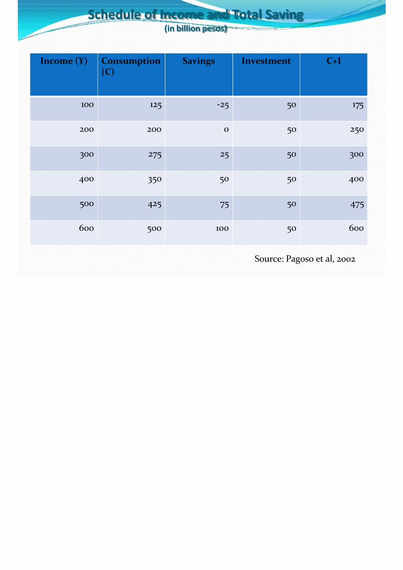
Schedule of Income and Total Saving(in billion pesos)
Income (Y) Consumption(C) Savings Investment C+I
100 125 -25 50 175
200 200 0 50 250
300 275 25 50 300
400 350 50 50 400
500 425 75 50 475
600 500 100 50 600
Source: Pagoso et al, 2002

8/2/2019 ECONOM1 Module 8 Natl Y Det
http://slidepdf.com/reader/full/econom1-module-8-natl-y-det 12/48
Income= Consumption+Investment
0
100
200
300
400
500
600
700
0 50 100 150 200 250 300 350 400 450 500 550 600
C+ I
C
Income
Y=C+S
C
-50
50
S
I
Y

8/2/2019 ECONOM1 Module 8 Natl Y Det
http://slidepdf.com/reader/full/econom1-module-8-natl-y-det 13/48
Investment Refers to the decision made by firms to spend on
capital goods
Determinants: economic factors, political conditions,peace and order situation, mood of investors
Components: business fixed investment, residentialconstruction, net change in business inventories

8/2/2019 ECONOM1 Module 8 Natl Y Det
http://slidepdf.com/reader/full/econom1-module-8-natl-y-det 14/48
Multiplier The number of times money has changed hands and
generate income
Multiplier K K = 1/(1-mpc)
Amount of Income Generated Yg = I x K

8/2/2019 ECONOM1 Module 8 Natl Y Det
http://slidepdf.com/reader/full/econom1-module-8-natl-y-det 15/48
Relevant Formulas & Symbols:
Y d = Disposable Income = Y Consumption Function: C = a + by (a= C at zero y or
the y-intercept; b=mpc or slope)
mpc = C rise
------ = --------- (slope of C function)
Y run
• Savings Function: S = Y – C
mps = S rise------ = --------- (slope of S function)
Y run
• mps + mpc = 1 S = Y - C

8/2/2019 ECONOM1 Module 8 Natl Y Det
http://slidepdf.com/reader/full/econom1-module-8-natl-y-det 16/48
Relevant Formulas & Symbols-contd:
M or K = 1 1--------- = ----------
1 – mpc mps , the multiplier
• Y = I x M or I x K• Yg = G x K

8/2/2019 ECONOM1 Module 8 Natl Y Det
http://slidepdf.com/reader/full/econom1-module-8-natl-y-det 17/48
A Demo Problem

8/2/2019 ECONOM1 Module 8 Natl Y Det
http://slidepdf.com/reader/full/econom1-module-8-natl-y-det 18/48
CENARIO 1 (SIMPLE ECONOMY): GNI = C + S
Given: a = P50B b = 75%
1. The Consumption Function: C = 50 + 0.75 y 2. Getting the Break-even Point (C=Y):
C = a + by
C = Y
a + by = Y
Y = a + by
Y = 50 + 0.75 y
(1 – 0.75) y = 50 Y = 50
----- = 200, the pt where c = Y
0.25
8/2/2019 ECONOM1 Module 8 Natl Y Det
http://slidepdf.com/reader/full/econom1-module-8-natl-y-det 19/48
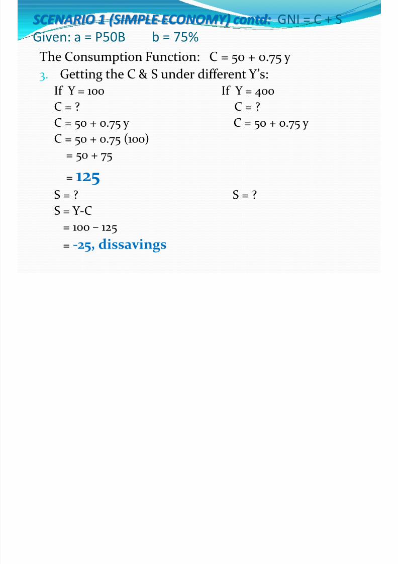
SCENARIO 1 (SIMPLE ECONOMY) contd: GNI = C + S
Given: a = P50B b = 75%
The Consumption Function: C = 50 + 0.75 y
3. Getting the C & S under different Y’s:
If Y = 100 If Y = 400
C = ? C = ?
C = 50 + 0.75 y C = 50 + 0.75 y C = 50 + 0.75 (100)
= 50 + 75
= 125S = ? S = ?S = Y-C
= 100 – 125
= -25, dissavings

8/2/2019 ECONOM1 Module 8 Natl Y Det
http://slidepdf.com/reader/full/econom1-module-8-natl-y-det 20/48
SCENARIO 1 (SIMPLE ECONOMY) contd: GNI = C + S
Given: a = P50B b = 75%
The Consumption Function: C = 50 + 0.75 y
3. Getting the C & S under different Y’s:
If Y = 100 If Y = 400
C = ? C = ?
C = 50 + 0.75 y C = 50 + 0.75 y C = 50 + 0.75 (100) = 50 + 0.75 (400)
= 50 + 75 = 50 + 300
= 125 = 350S = ? S = ?S = Y-C = Y - C
= 100 – 125 = 400 - 350
= -25, dissavings = 50, + savings
8/2/2019 ECONOM1 Module 8 Natl Y Det
http://slidepdf.com/reader/full/econom1-module-8-natl-y-det 21/48
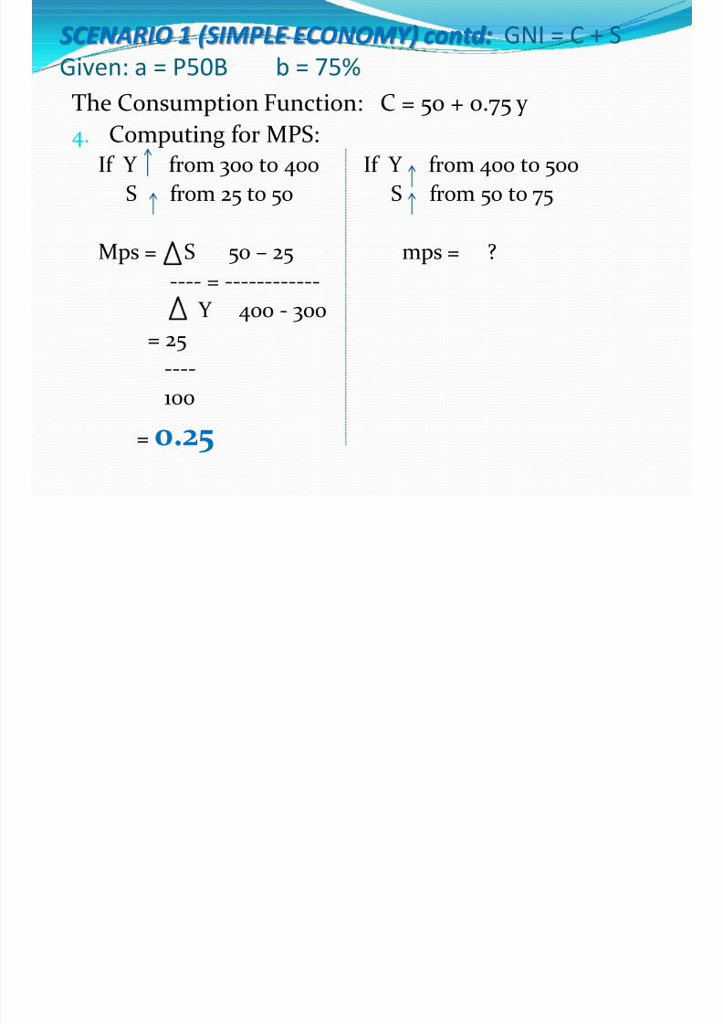
SCENARIO 1 (SIMPLE ECONOMY) contd: GNI = C + S
Given: a = P50B b = 75%
The Consumption Function: C = 50 + 0.75 y
4. Computing for MPS:If Y from 300 t0 400 If Y from 400 to 500
S from 25 to 50 S from 50 to 75
Mps = S 50 – 25 mps = ?
---- = ------------
Y 400 - 300
= 25----
100
= 0.25
8/2/2019 ECONOM1 Module 8 Natl Y Det
http://slidepdf.com/reader/full/econom1-module-8-natl-y-det 22/48
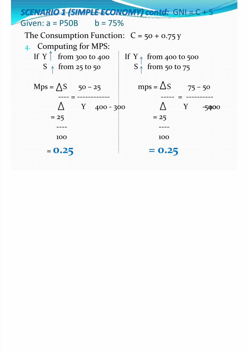
SCENARIO 1 (SIMPLE ECONOMY) contd: GNI = C + S
Given: a = P50B b = 75%
The Consumption Function: C = 50 + 0.75 y
4. Computing for MPS:If Y from 300 t0 400 If Y from 400 to 500
S from 25 to 50 S from 50 to 75
Mps = S 50 – 25 mps = S 75 – 50
---- = ------------ ----- = ----------
Y 400 - 300 Y 500– 400
= 25 = 25---- ----
100 100
= 0.25 = 0.25
( )

8/2/2019 ECONOM1 Module 8 Natl Y Det
http://slidepdf.com/reader/full/econom1-module-8-natl-y-det 23/48
CENARIO 2 (ECONOMY w HH & investors):
(GNI = C + I)
Given: a = P50B b = 75% I = 501. Solving for equilibrium Y when there are values for C & I
Y = C + I, C = a + by
Y = a + by + I
Y = 50 + 0.75 y + 50 Y – 0.75 y = 100
0.25 y = 100
Y = 400, the equilibrium income
8/2/2019 ECONOM1 Module 8 Natl Y Det
http://slidepdf.com/reader/full/econom1-module-8-natl-y-det 24/48
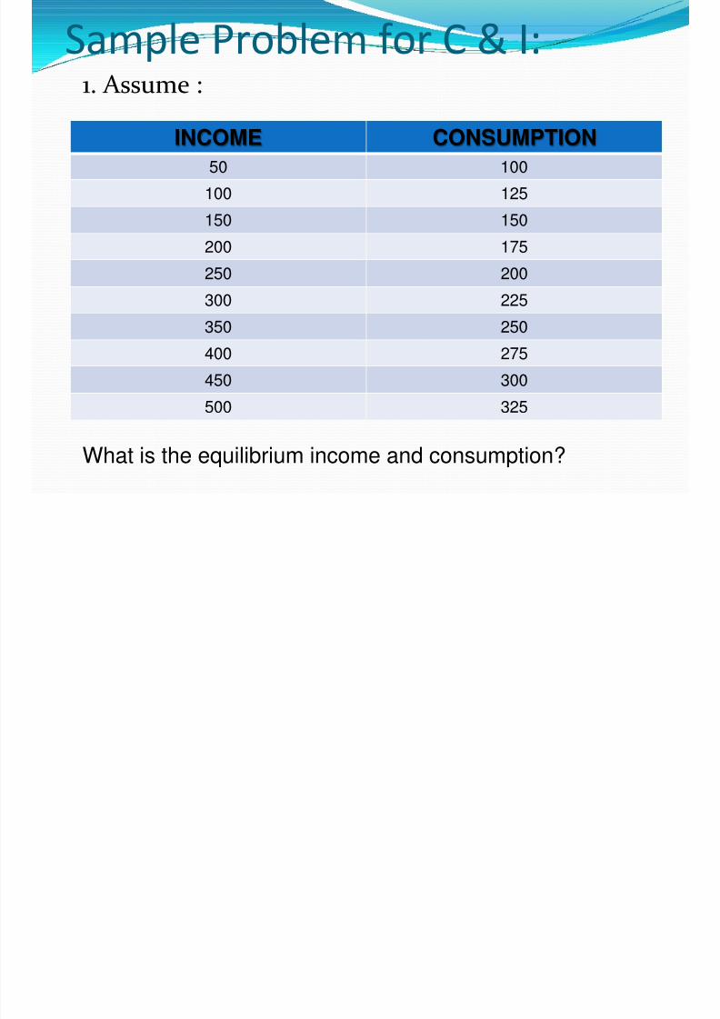
Sample Problem for C & I:
INCOME CONSUMPTION
50 100
100 125
150 150
200 175
250 200
300 225
350 250
400 275
450 300
500 325
1. Assume :
What is the equilibrium income and consumption?
8/2/2019 ECONOM1 Module 8 Natl Y Det
http://slidepdf.com/reader/full/econom1-module-8-natl-y-det 25/48
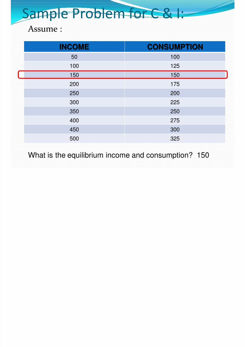
Sample Problem for C & I:
INCOME CONSUMPTION
50 100
100 125
150 150
200 175
250 200
300 225
350 250
400 275
450 300
500 325
Assume :
What is the equilibrium income and consumption? 150

8/2/2019 ECONOM1 Module 8 Natl Y Det
http://slidepdf.com/reader/full/econom1-module-8-natl-y-det 26/48
Sample Problem for C & I:
INCOME CONSUMPTION
INVESTMENT
C + I
50 100
100 125
150 150
200 175
250 200
300 225
350 250
400 275
450 300
500 325
2. Construct a new schedule with investment equal to 25:
What is the new equilibrium income?

8/2/2019 ECONOM1 Module 8 Natl Y Det
http://slidepdf.com/reader/full/econom1-module-8-natl-y-det 27/48
Sample Problem for C & I:
INCOME CONSUMPTION
INVESTMENT
C + I
50 100 25 125
100 125 25 150
150 150 25 175
200 175 25 200
250 200 25 225
300 225 25 250
350 250 25 275
400 275 25 300
450 300 25 325
500 325 25 350
2. Construct a new schedule with investment equal to 25:
What is the new equilibrium income? 200
Sample Problem for C & I:

8/2/2019 ECONOM1 Module 8 Natl Y Det
http://slidepdf.com/reader/full/econom1-module-8-natl-y-det 28/48
Sample Problem for C & I:
INCOME CONSUMPTION INVESTMENT C + I
50 100 25 125
100 125 25 150
150 150 25 175
200 175 25 200
250 200 25 225
300 225 25 250
350 250 25 275
400 275 25 300
450 300 25 325
500 325 25 350
2. Construct a new schedule with investment equal to 25:
What is the new equilibrium income? 200
CHECK: mpc = 0.5 , mps = 0.5, M = 1 / 0.5 = 2, Y = I x M = 25 x 2 = 50Ye (new) = 150 + 50 = 200
Sample Problem for C & I:

8/2/2019 ECONOM1 Module 8 Natl Y Det
http://slidepdf.com/reader/full/econom1-module-8-natl-y-det 29/48
Sample Problem for C & I:3. Assume Y = 50, C = 40, I = 10, mps = 0.2, M = ?
Sample Problem for C & I:

8/2/2019 ECONOM1 Module 8 Natl Y Det
http://slidepdf.com/reader/full/econom1-module-8-natl-y-det 30/48
Sample Problem for C & I:3. Assume Y = 50, C = 40, I = 10, mps = 0.2, M = ?
M = 1 / mps = 1 / 0.2 = 5
a. What would be additional Income and Consumption if Investmentwere to increase by 7.5?
Sample Problem for C & I:

8/2/2019 ECONOM1 Module 8 Natl Y Det
http://slidepdf.com/reader/full/econom1-module-8-natl-y-det 31/48
Sample Problem for C & I:3. Assume Y = 50, C = 40, I = 10, mps = 0.2, M = ?
M = 1 / mps = 1 / 0.2 = 5
a. What would be additional Income and Consumption if Investmentwere to increase by 7.5?
Y = add’l I x K = 7.5 x 5 = 37.5, the additional Y
Y C I S (Y-C)
I = 10 50 40 10 _______
I = 17.5 ________ _______ _______ _______
Sample Problem for C & I:

8/2/2019 ECONOM1 Module 8 Natl Y Det
http://slidepdf.com/reader/full/econom1-module-8-natl-y-det 32/48
Sample Problem for C & I:3. Assume Y = 50, C = 40, I = 10, mps = 0.2, M = ?
M = 1 / mps = 1 / 0.2 = 5
a. What would be additional Income and Consumption if Investmentwere to increase by 7.5?
Y = add’l I x K = 7.5 x 5 = 37.5, the additional Y
b. What would be total Y and C as a result of the foregoing?
Y C I S (Y-C)
I = 10 50 40 10 10
I = 17.5 _______ _______ _______ _______
(1)
Sample Problem for C & I:

8/2/2019 ECONOM1 Module 8 Natl Y Det
http://slidepdf.com/reader/full/econom1-module-8-natl-y-det 33/48
Sample Problem for C & I:3. Assume Y = 50, C = 40, I = 10, mps = 0.2, M = ?
M = 1 / mps = 1 / 0.2 = 5
a. What would be additional Income and Consumption if Investmentwere to increase by 7.5?
Y = add’l I x K = 7.5 x 5 = 37.5, the additional Y
b. What would be total Y and C as a result of the foregoing?Yt = Y 1 + Y = 50 + 37.5 = 87.5, total Y
Y = C + I, C = Y – IC = 87.5 – 17.5 = 70, total C
Y C I S (Y-C)
I = 10 50 40 10 10
I = 17.5 87.5 70 17.5 _______
(1)
(2) (50+37.5) (3)(10+7.5)(4)(87.5-17.5)
Sample Problem for C & I:

8/2/2019 ECONOM1 Module 8 Natl Y Det
http://slidepdf.com/reader/full/econom1-module-8-natl-y-det 34/48
Sample Problem for C & I:3. Assume Y = 50, C = 40, I = 10, mps = 0.2, M = ?
M = 1 / mps = 1 / 0.2 = 5
a. What would be additional Income and Consumption if Investment were to increase
by 7.5?
Y = add’l I x K = 7.5 x 5 = 37.5, the additional Y
b. What would be total Y and C as a result of the foregoing?Yt = Y 1 + Y = 50 + 37.5 = 87.5, total Y
Y = C + I, C = Y – IC = 87.5 – 17.5 = 70, total C
c. Compute Additional Savings
Y C I S (Y-C)
I = 10 50 40 10 10
I = 17.5 87.5 70 17.5 _______
(1)
(2)(50+37.5) (3)(10+7.5)(4)(87.5-17.5)
Sample Problem for C & I:

8/2/2019 ECONOM1 Module 8 Natl Y Det
http://slidepdf.com/reader/full/econom1-module-8-natl-y-det 35/48
Sample Problem for C & I:3. Assume Y = 50, C = 40, I = 10, mps = 0.2, M = ?
M = 1 / mps = 1 / 0.2 = 5
a. What would be additional Income and Consumption if Investment were to increase
by 7.5?
Y = add’l I x K = 7.5 x 5 = 37.5, the additional Y
b. What would be total Y and C as a result of the foregoing?Yt = Y 1 + Y = 50 + 37.5 = 87.5, total Y
Y = C + I, C = Y – IC = 87.5 – 17.5 = 70, total C
c. Compute Additional SavingsS = Y – C = 87.5 -70 = 17.5
S = Snew – Sold = 17.5 – 10 = 7.5, additional S
Y C I S (Y-C)
I = 10 50 40 10 10
I = 17.5 87.5 70 17.5 17.5
(1)
(2)(50+37.5) (3)(10+7.5)
(4)
(87.5-17.5) (5)

8/2/2019 ECONOM1 Module 8 Natl Y Det
http://slidepdf.com/reader/full/econom1-module-8-natl-y-det 36/48
Reminder: Submission of Take-
home quiz on C & I function isnext meeting

8/2/2019 ECONOM1 Module 8 Natl Y Det
http://slidepdf.com/reader/full/econom1-module-8-natl-y-det 37/48
CENARIO 3 (ECONOMY w HH & investors &
Government):
(GNI = C + I + G)Given: a = P50B b = 75% I = 50 Yg=100
1. Solving for full employment equilibrium Y when there
are values for C & I & G can be computed

8/2/2019 ECONOM1 Module 8 Natl Y Det
http://slidepdf.com/reader/full/econom1-module-8-natl-y-det 38/48
CENARIO 3 (ECONOMY w HH & investors &
Government):
(GNI = C + I + G)Given: a = P50B b = 75% I = 50 Yg=100
1. Solving for full employment equilibrium Y when there
are values for C & I & G can be computed Yg = G x K, M or K = 1 / 1-mpc = 1/ 1-0.75 = 1/0.25 = 4
100 = G x 4
G = 100 / 4 = 25, the Government Spending G
Y = a + by + I + G = 50 + 0.75 y + 50 + 25
= 125 + 0.75 y
(y – 0.75y) = 125
Y = 500, the full employment equilibrium Ye
(
8/2/2019 ECONOM1 Module 8 Natl Y Det
http://slidepdf.com/reader/full/econom1-module-8-natl-y-det 39/48
CENARIO 3 (ECONOMY w HH & investors &
Government – cont’d):
(GNI = C + I + G)Given: a = P50B, b = 75%, I = 50, Yg=100, G=25, Ye =500
Y,C,C+I,C+I+G
Y
P i E i (ECONOMY HH &

8/2/2019 ECONOM1 Module 8 Natl Y Det
http://slidepdf.com/reader/full/econom1-module-8-natl-y-det 40/48
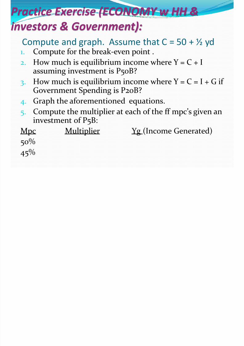
Practice Exercise (ECONOMY w HH &
investors & Government):
Compute and graph. Assume that C = 50 + ½ yd1. Compute for the break-even point .
2. How much is equilibrium income where Y = C + Iassuming investment is P50B?
3. How much is equilibrium income where Y = C = I + G if Government Spending is P20B?
4. Graph the aforementioned equations.
5. Compute the multiplier at each of the ff mpc’s given an
investment of P5B:Mpc Multiplier Yg (Income Generated)
50%
45%

8/2/2019 ECONOM1 Module 8 Natl Y Det
http://slidepdf.com/reader/full/econom1-module-8-natl-y-det 41/48
Government Spending As determined from the HH,
investors, and government sectors, Y = C + I + G, G is value of government
spending (Yg= G x K)

8/2/2019 ECONOM1 Module 8 Natl Y Det
http://slidepdf.com/reader/full/econom1-module-8-natl-y-det 42/48
Full Employment Equilibrium The level of income where there is no
available and useful resource that is wasted

8/2/2019 ECONOM1 Module 8 Natl Y Det
http://slidepdf.com/reader/full/econom1-module-8-natl-y-det 43/48
Inflationary Gap Occurs when aggregate demand C + I + G exceeds
equilibrium income Y
Deflationary GapOccurs when aggregate demand C + I + G fall short of equilibrium income Y

8/2/2019 ECONOM1 Module 8 Natl Y Det
http://slidepdf.com/reader/full/econom1-module-8-natl-y-det 44/48
Schedule of Income and Total Spending (in billion pesos)
Y C I G C+I + G
100 125 50 25 200
200 200 50 25 275
300 275 50 25 350
400 350 50 25 425
500 425 50 25 500
Source: Pagoso et al, 2002

8/2/2019 ECONOM1 Module 8 Natl Y Det
http://slidepdf.com/reader/full/econom1-module-8-natl-y-det 45/48
Full Employment Equilibrium
0
100
200
300
400
500
600
700
0 50 100 150 200 250 300 350 400 450 500 550 600
C+ I
C
Income
Y=C+S
C
-50
50
S
I
Y
C+I+G

8/2/2019 ECONOM1 Module 8 Natl Y Det
http://slidepdf.com/reader/full/econom1-module-8-natl-y-det 46/48
Fiscal Policy When the government uses its powers to influence
total spending either directly by changingits purchasesof goods and services or indirectly by altering the
disposable incomes of persons to changes in the levelof taxation or transfer outlays

8/2/2019 ECONOM1 Module 8 Natl Y Det
http://slidepdf.com/reader/full/econom1-module-8-natl-y-det 47/48
Fiscal Policies
1) Periods of deflationDeficit budget (government spending more than
what it collects through taxes) or tax cuts
2) Periods of inflationSurplus budget (government spending less than its
budget) or balanced budget or tax increases
Major Macroeconomic Effects of

8/2/2019 ECONOM1 Module 8 Natl Y Det
http://slidepdf.com/reader/full/econom1-module-8-natl-y-det 48/48
Major Macroeconomic Effects of
Government Expenditure and Tax
Policy
The Expenditure Impact
The Financial Impact
The Supply Impact