ECON 311 MICROECONOMICS THEORY I · ECON 311 MICROECONOMICS THEORY I ... profit by choosing the...

ECON 311

MICROECONOMICS THEORY I

Profit Maximisation &

Perfect Competition (Short-Run)

Dr. F. Kwame Agyire-Tettey Department of Economics

Contact Information: [email protected]

Session Overview

• Given that it has desirable properties, perfect competition isuseful for comparison with other market structure. Thissession presents an introduction to market structures andperfect competition. It also looks at the profit maximizationconditions of a firm as well as the perfect competitive short-run equilibrium.

Slide 2

Session Outline

• Profit maximization condition of the firm

– Output choice

– Marginal revenue and price elasticity

• Introduction to Market Structure and Perfect Competition

– Market Structures

– Perfectly Competitive Market

• Competition in the Short-run

– Demand Curve

– Profit maximization

– Supply Curve

– Competitive Industry EquilibriumSlide 3

Learning Outcome

After this session, you should be able to;

• Explain the concept of market structure.

• Outline the major assumptions of the perfectly competitivefirm.

• Understand how competitive firms maximize profit in theshort-run.

• Explain the short-run competitive demand and supply curve.

• Understand competitive equilibrium in the Short Run.

Slide 4

Reading List

• Read Chapter 8 of Jeffrey M. Perfloff (2012).Microeconomics (Sixth edition), Pearson Education Ltd.

• Read Chapter 23 and 24 of Hal R. Varian (2014).Intermediate Microeconomics, W. W. Norton andCompany.

• Session slides

• Any other Economics textbook

Slide 5

6

Modeling Firms’ Behaviour

• Economists see firms as single decision-making unit– decisions are made by a single “dictatorial” manager who

rationally pursues some goal - profit maximization

• A profit-maximizing firm chooses both its inputs and outputs with the sole goal of maximising profits– seeks to maximize the difference between total revenue and total

economic costs

• If firms are strictly profit maximizers, they will make decisions in a “marginal” way– examine the marginal profit obtainable from producing one more

unit of hiring one additional labourer

7

Output Choice

• Total revenue (TR) for a firm is given by

R(q) = p(q)q

• In the production of q, certain economic costs are incurred [C(q)]

• Economic profits () are the difference between total revenue and total costs (TC)

(q) = R(q) – C(q) = p(q)q –C(q)

8

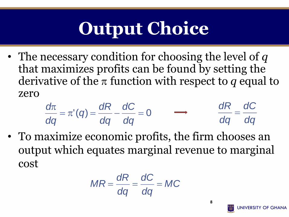
Output Choice

• The necessary condition for choosing the level of qthat maximizes profits can be found by setting the derivative of the function with respect to q equal to zero

0)('

dq

dC

dq

dRq

dq

d

dq

dC

dq

dR

• To maximize economic profits, the firm chooses an output which equates marginal revenue to marginal cost

MCdq

dC

dq

dRMR

9

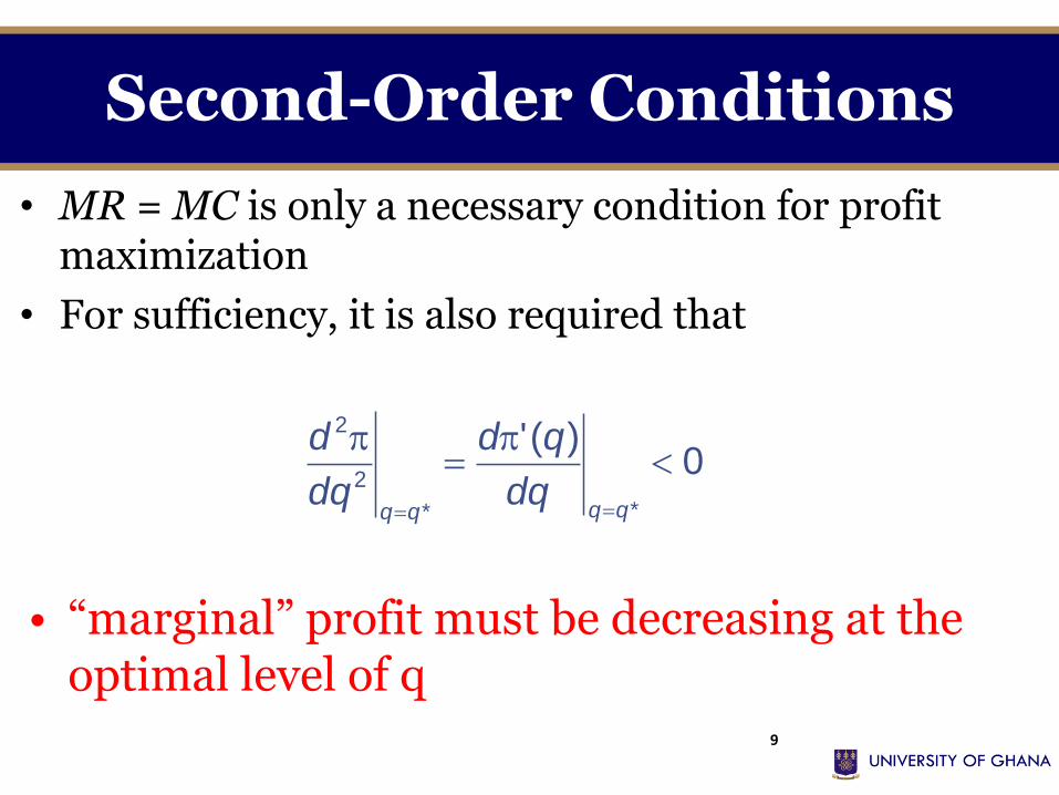
Second-Order Conditions

• MR = MC is only a necessary condition for profit maximization

• For sufficiency, it is also required that

0)('

**

2

2

qqqqdq

qd

dq

d

• “marginal” profit must be decreasing at the optimal level of q

10

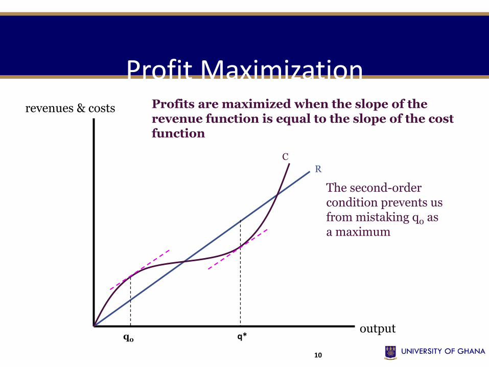
Profit Maximization

output

revenues & costs

R

C

q*

Profits are maximized when the slope of the revenue function is equal to the slope of the cost function

The second-order condition prevents usfrom mistaking q0 asa maximum

q0

11

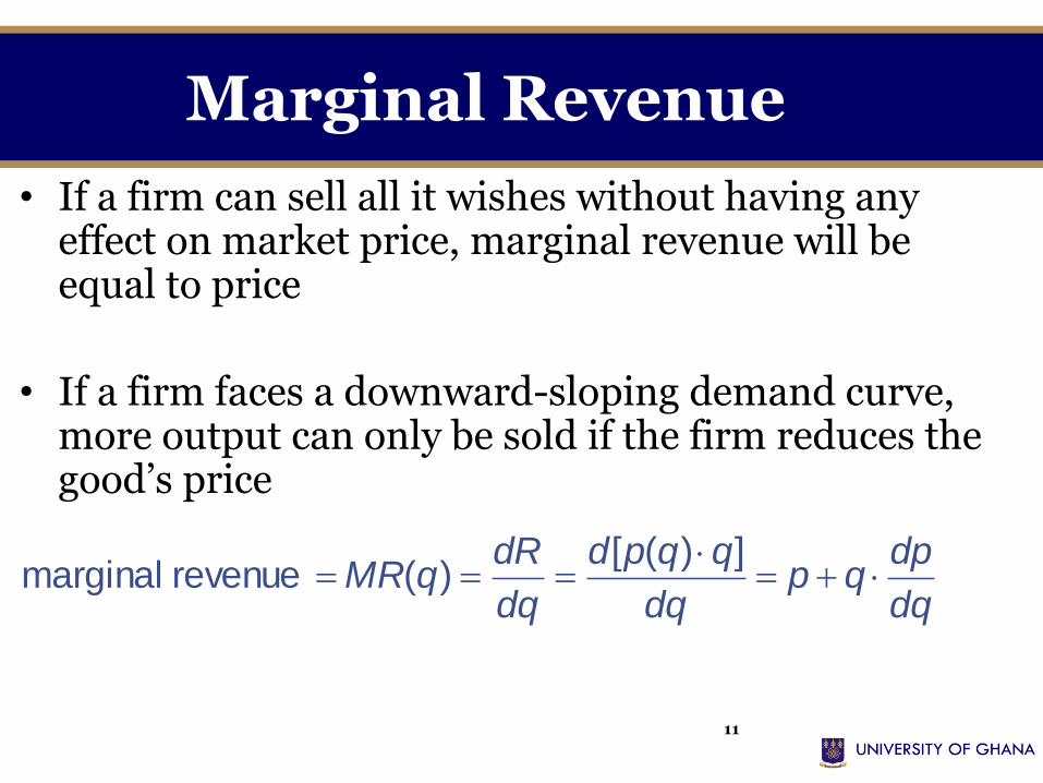
Marginal Revenue

• If a firm can sell all it wishes without having any effect on market price, marginal revenue will be equal to price

• If a firm faces a downward-sloping demand curve, more output can only be sold if the firm reduces the good’s price

dq

dpqp

dq

qqpd

dq

dRqMR

])([)( revenue marginal

12

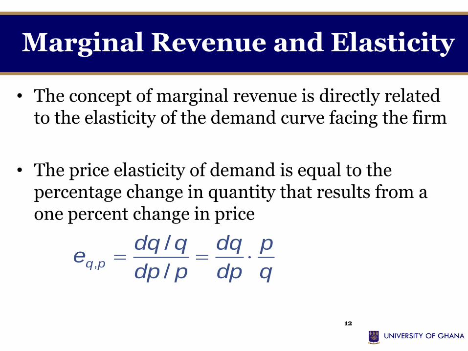
Marginal Revenue and Elasticity

• The concept of marginal revenue is directly related to the elasticity of the demand curve facing the firm

• The price elasticity of demand is equal to the percentage change in quantity that results from a one percent change in price

q

p

dp

dq

pdp

qdqe pq

/

/,

13

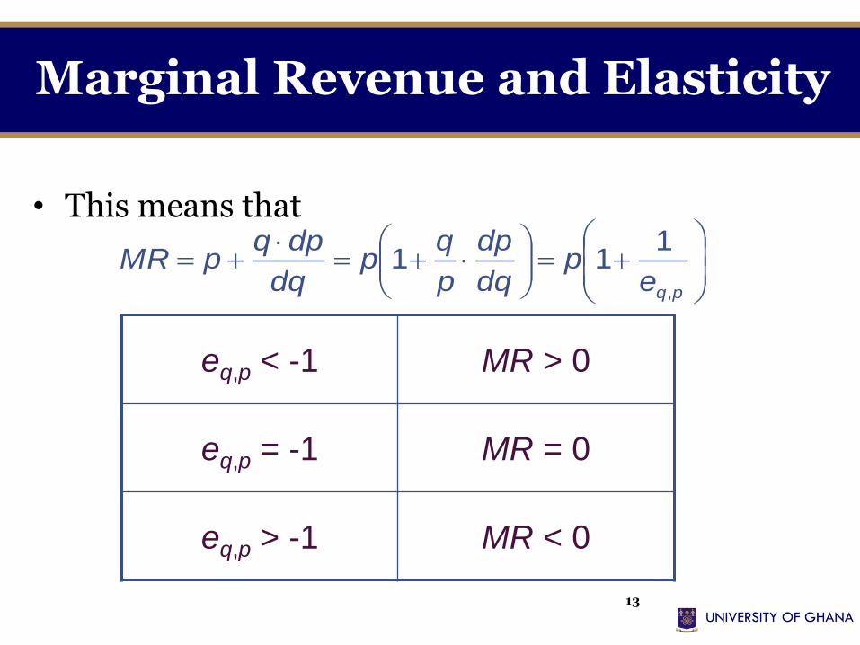
Marginal Revenue and Elasticity

• This means that

pqep

dq

dp

p

qp

dq

dpqpMR

,

111

eq,p < -1 MR > 0

eq,p = -1 MR = 0

eq,p > -1 MR < 0

14

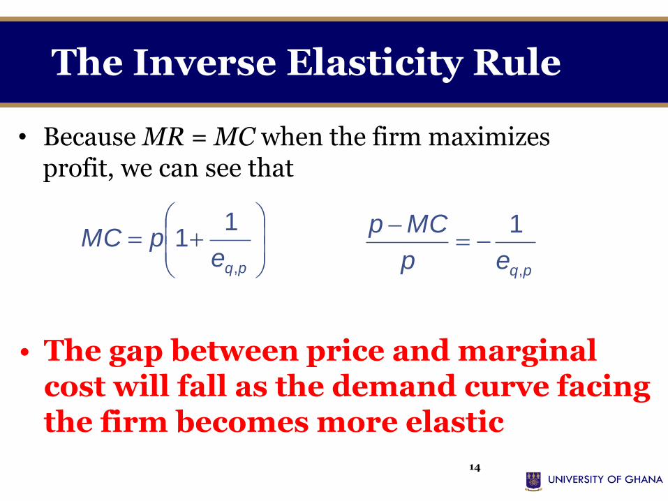
The Inverse Elasticity Rule

• Because MR = MC when the firm maximizes profit, we can see that

pqepMC

,

11

pqep

MCp

,

1

• The gap between price and marginal cost will fall as the demand curve facing the firm becomes more elastic

Introduction to Market Structures

Slide 15

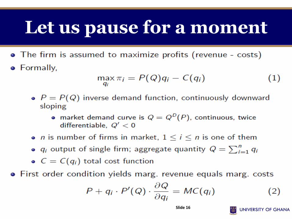
Let us pause for a moment

Slide 16

Introduction(Market Structure)

• Market structure explains how firms in the market behavebased on the market demand of consumers. It is defined by thecharacteristics that influence the behaviour and outcomes ofthe firms activities in that market.

• Several market structures exist. Examples include:

– Perfect competition

– imperfect competition

– monopoly

– oligopoly

– duopoly

– monopolistic competition

Slide 17

Introduction (Market Structure)

• The structure of the market is determined by the followingfactors:

– Number of economic agents in the market (both sellers andbuyers).

– Relative negotiation strength of the economic agents in termsof ability to set prices.

– Degree of concentration among the economic agents.

– Degree of product differentiation and homogeneity.

– Degree of barriers to entry and exit.

Slide 18

Introduction (Perfectly Competitive Market)

• When there is a rivalry among the firms in the market for thesame customers, they are termed as “competitive firms”.

• In that regard, a perfectly competitive market is a market inwhich there are large number of competitive firms such that it isdifficult to single out a firm as an opponent.

• Perfect competition occurs where firms have no marketpower and hence do not react to each other.

• Examples of perfectly competitively markets include; market for many agricultural produce; stock exchange markets; retail and wholesale markets; among others.

Slide 19


• Assumptions of Perfect Competition (Why demand curve ishorizontal):

1. Firms sell homogenous or identical products;

2. Large number of sellers and buyers;

3. Free entry and exit;

4. Full information/Perfect knowledge;

5. Negligible/low transaction costs;

6. Perfect mobility of productive resources.

Note: The first two assumptions make competitive firms price-takers. Ifany competitive firm attempts to charge a higher price, its customers willbuy the same product from elsewhere. Hence, there is no incentive tolower the price of a good since the firm can sell as many goods as possibleat that market price.

Slide 20


• The perfectly competitive firm faces a demand curve that is horizontal(perfectly/infinitely elastic) at the market price. The choice of the quantityof output to sell has no effect on price. Therefore, the firm can sell as manyunits of goods/output as it desires at the set market price, 𝑝.

• To maximize profit, a competitive firm ought to produce an output levelthat equates marginal cost (𝑀𝐶) to marginal revenue (𝑀𝑅); where 𝑀𝑅equals market price (P). Also, 𝑀𝐶 should be rising or by producingnothing if average cost exceeds price at all outputs.

𝑀𝐶(𝑞) =𝑀𝑅(𝑞)=P

• Therefore, a perfectly competitive firm is a quantity-adjuster, facing aperfectly elastic demand curve at the given market price and maximizingprofit by choosing the output that equates its marginal cost to themarket price.

Slide 21

Competition in the Short-run(Demand Curve)

Slide 22

𝐷𝑓𝑖𝑟𝑚 = 𝐴𝑅 = 𝑀𝑅 = 𝑃

Q

Price

Quantity

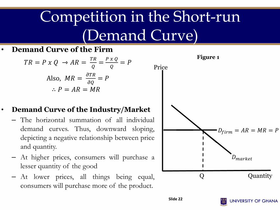
• Demand Curve of the Firm

𝑇𝑅 = 𝑃 𝑥 𝑄 ⇾ 𝐴𝑅 =𝑇𝑅

𝑄=

𝑃 𝑥 𝑄

𝑄= 𝑃

Also, 𝑀𝑅 =𝜕𝑇𝑅

𝜕𝑄= 𝑃

∴ 𝑃 = 𝐴𝑅 = 𝑀𝑅

• Demand Curve of the Industry/Market

– The horizontal summation of all individual

demand curves. Thus, downward sloping,

depicting a negative relationship between price

and quantity.

– At higher prices, consumers will purchase a

lesser quantity of the good

– At lower prices, all things being equal,

consumers will purchase more of the product.

Figure 1

𝐷𝑚𝑎𝑟𝑘𝑒𝑡

Competition in the Short-run (Profit Maximization)

• Economists usually assume that the goal of all firms (not onlycompetitive firms) is profit maximization.

• A firm’s profit (𝜋) is defined by the difference between its total revenue(TR) and total cost (TC). The TC considered is the economics cost. Thisconstitutes both explicit and implicit costs. Profit is representedmathematically as;

𝜋 (q) = TR (q) – TC (q)

𝜕𝜋

𝜕𝑞=

𝜕𝑇𝑅

𝜕𝑞=

𝜕𝑇𝐶

𝜕𝑞= 0

• Hence, the first-order condition (FOC) for profit maximization is,𝑀𝑅 (𝑠𝑙𝑜𝑝𝑒 𝑜𝑓 𝑇𝑅 𝑐𝑢𝑟𝑣𝑒)=𝑀𝐶 (𝑠𝑙𝑜𝑝𝑒 𝑜𝑓 𝑇𝐶 𝑐𝑢𝑟𝑣𝑒) . Since 𝑀𝑅 = 𝑃, theFOC might be written as 𝑀𝐶 = 𝑃.

Slide 23


• The second-order condition (SOC) for profit maximization requiresthat the second derivative of the profit function be negative. This isgiven as:

𝜕2𝜋

𝜕𝑞2=𝜕2𝑇𝑅

𝜕𝑞2−𝜕2𝑇𝐶

𝜕𝑞2< 0

• Thus, 𝜕2𝑇𝑅

𝜕𝑞2(𝑠𝑙𝑜𝑝𝑒 𝑜𝑓 𝑀𝑅 𝑐𝑢𝑟𝑣𝑒) <

𝜕2𝑇𝐶

𝜕𝑞2(𝑠𝑙𝑜𝑝𝑒 𝑜𝑓 𝑀𝐶 𝑐𝑢𝑟𝑣𝑒). The SOC

therefore requires that the slope of the 𝑀𝐶 curve to be steeper than that of the 𝑀𝑅 curve or the 𝑀𝐶 curve must cut the 𝑀𝑅 curve from below. In perfect competition, the slope of the MR curve is zero; resultantly, the SOC requires that the 𝑀𝐶 curve must have a positive/rising slope. This (SOC) is simplified as:

0 < 𝜕2𝑇𝐶

𝜕𝑞2

Slide 24


Slide 25

TCTR

400

244

0

50

100

150

200

250

300

350

400

450

500

550

600

0 1 2 3 4 5 6 7 8 9 10 11 12

Q

MC

MR

0

10

20

30

40

50

60

70

80

90

100

110

120

130

140

150

0 1 2 3 4 5 6 7 8 9 10 11 12Q

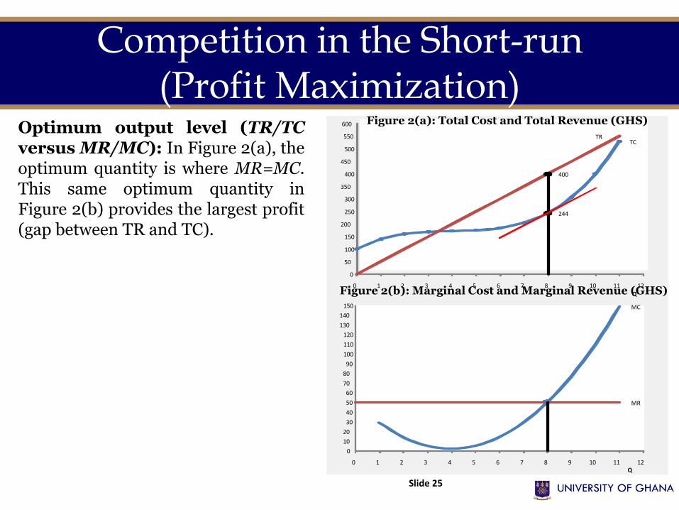
Optimum output level (TR/TCversus MR/MC): In Figure 2(a), theoptimum quantity is where MR=MC.This same optimum quantity inFigure 2(b) provides the largest profit(gap between TR and TC).

Figure 2(a): Total Cost and Total Revenue (GHS)

Figure 2(b): Marginal Cost and Marginal Revenue (GHS)


Slide 26

TC TR

0

To

tal

cost

, re

ven

ue

(GH

C)

385350315280245210175140105

7035

Quantity1 2 3 4 5 6 7 8 9

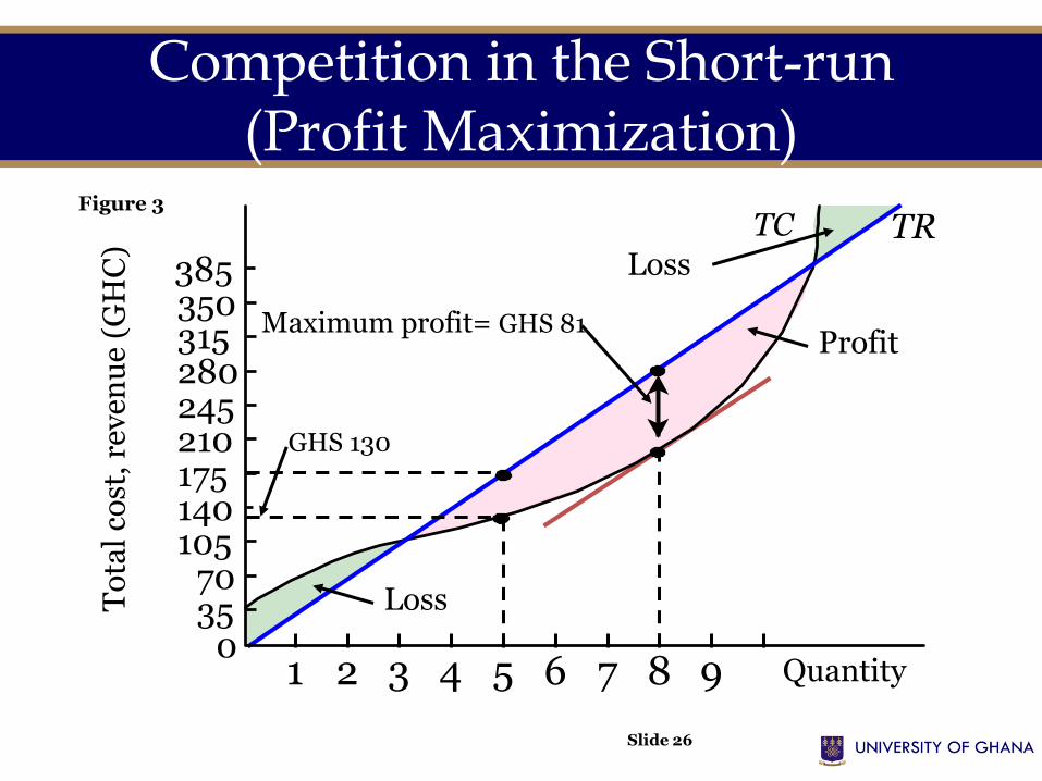
Maximum profit= GHS 81

GHS 130

Loss

Loss

Profit

Figure 3

Profit Maximization

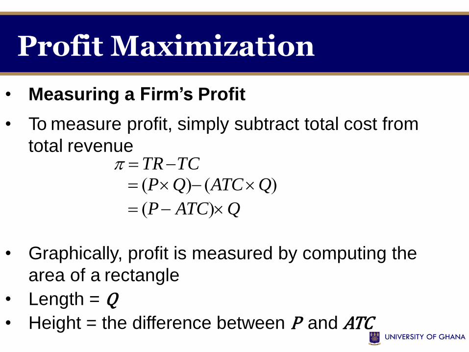
• Measuring a Firm’s Profit

• To measure profit, simply subtract total cost from

total revenue TRTC

PQ ATCQ

P ATCQ

• Graphically, profit is measured by computing the

area of a rectangle

• Length = Q• Height = the difference between P and ATC


Slide 28

MC

P

Price

QuantityQ

ATC

AVC

Total Cost

D=MR=PProfit

Economic Profit (P > ATC):Here, the return on the existingallocation exceeds its opportunitycost.

Figure 4


Slide 29

MC

P

Price

QuantityQ

ATC

AVC

Total Cost = Total Revenue

D=MR=P

Normal Profit (P = ATC): Thisis the breakeven profit where firmsearn zero economic profit butnormal profit. Normal profit iswhere the firm earns fair profit,such that the returns from exitingallocation is not different from itsopportunity cost.

Figure 5


Slide 30

MC

P

Price

QuantityQ

ATC

AVC

Total Cost

D=MR=PLoss

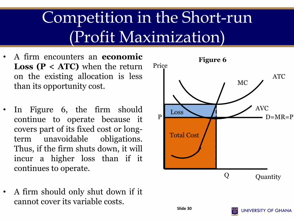
• A firm encounters an economicLoss (P < ATC) when the returnon the existing allocation is lessthan its opportunity cost.

• In Figure 6, the firm shouldcontinue to operate because itcovers part of its fixed cost or long-term unavoidable obligations.Thus, if the firm shuts down, it willincur a higher loss than if itcontinues to operate.

• A firm should only shut down if itcannot cover its variable costs.

Figure 6

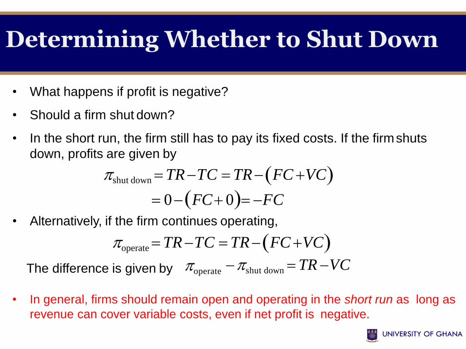
The difference is given by

• In general, firms should remain open and operating in the short run as long as

revenue can cover variable costs, even if net profit is negative.

• What happens if profit is negative?

• Should a firm shut down?

• In the short run, the firm still has to pay its fixed costs. If the firmshuts

down, profits are given by

shut down TRTC TR FC VC

0 FC 0 FC

• Alternatively, if the firm continues operating,

operateTRTC TRFC VCoperate

shut down TR VC

Determining Whether to Shut Down


ATCMCPrice

& cost (¢/unit)

ATC* AVC

d = MRP*

AVC*

QuantityQ*

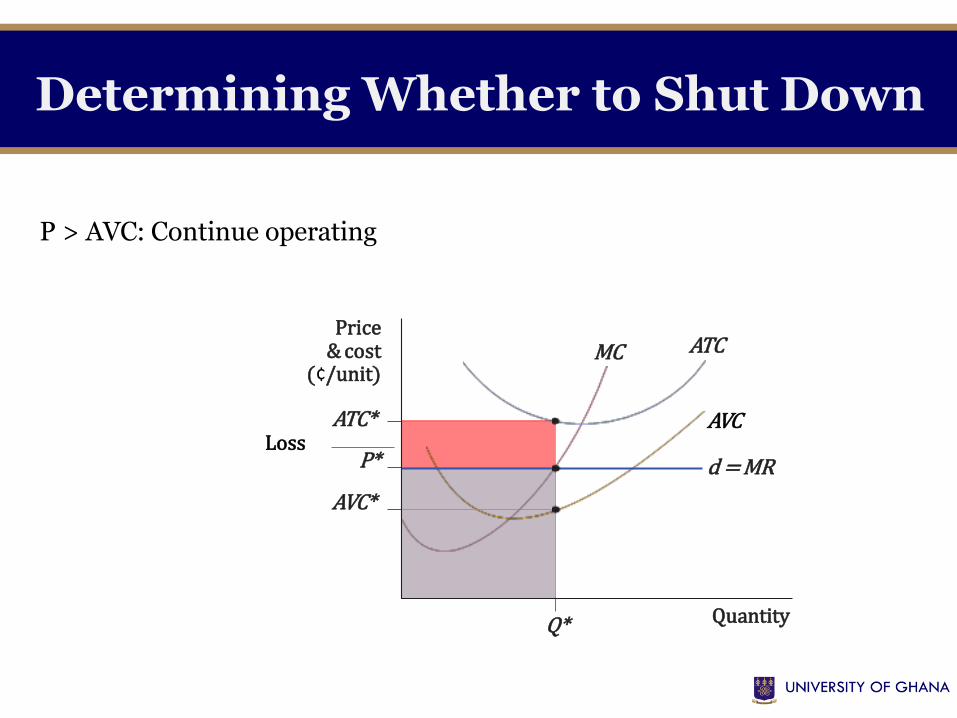
P > AVC: Continue operating

Loss


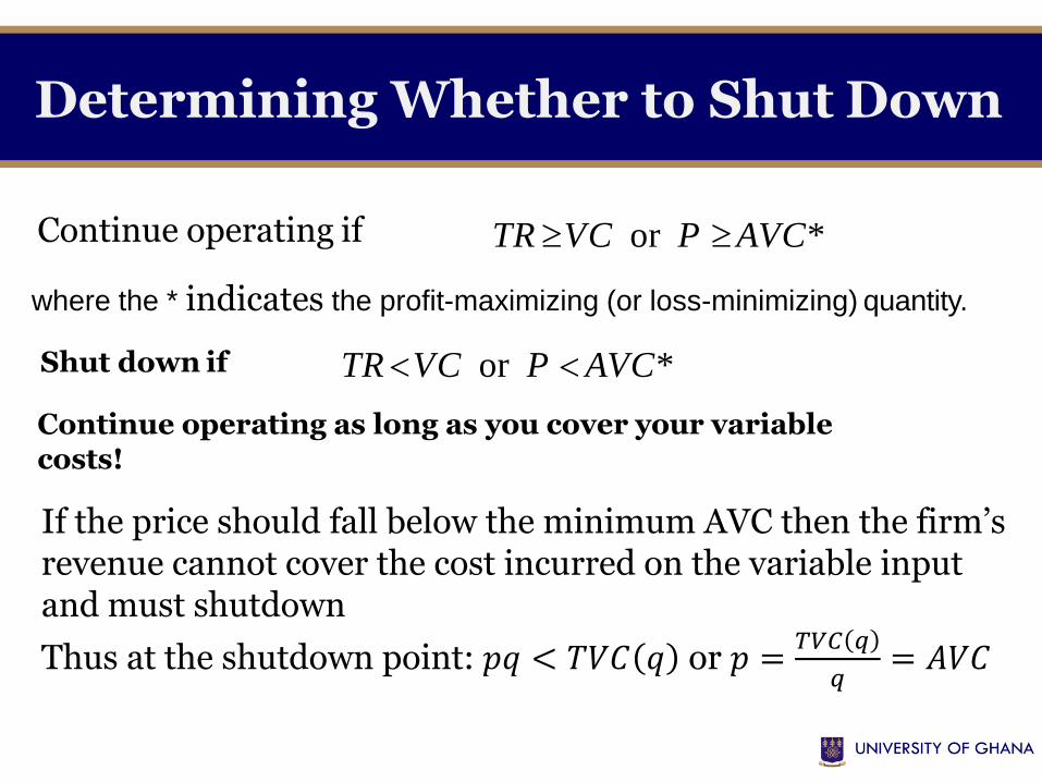
Continue operating if

where the * indicates the profit-maximizing (or loss-minimizing) quantity.

Shut down if

Continue operating as long as you cover your variablecosts!

TR VC or P AVC*

TR VC or P AVC*

If the price should fall below the minimum AVC then the firm’s revenue cannot cover the cost incurred on the variable input and must shutdown

Thus at the shutdown point: 𝑝𝑞 < 𝑇𝑉𝐶 𝑞 or 𝑝 =𝑇𝑉𝐶 𝑞

𝑞= 𝐴𝑉𝐶

Competition in the Short-run (Supply Curve)

Slide 34

1

2

3

4

5

Quantity

GH

S p

er

nu

t

1

2

3

QuantityFigure 7. Marginal cost and average variable cost curves Figure 8. The supply curve

p0E0

MC

q0

AVC

q1

4

q2

5

S

E1 p1

E2 p2

E3 p3

q3


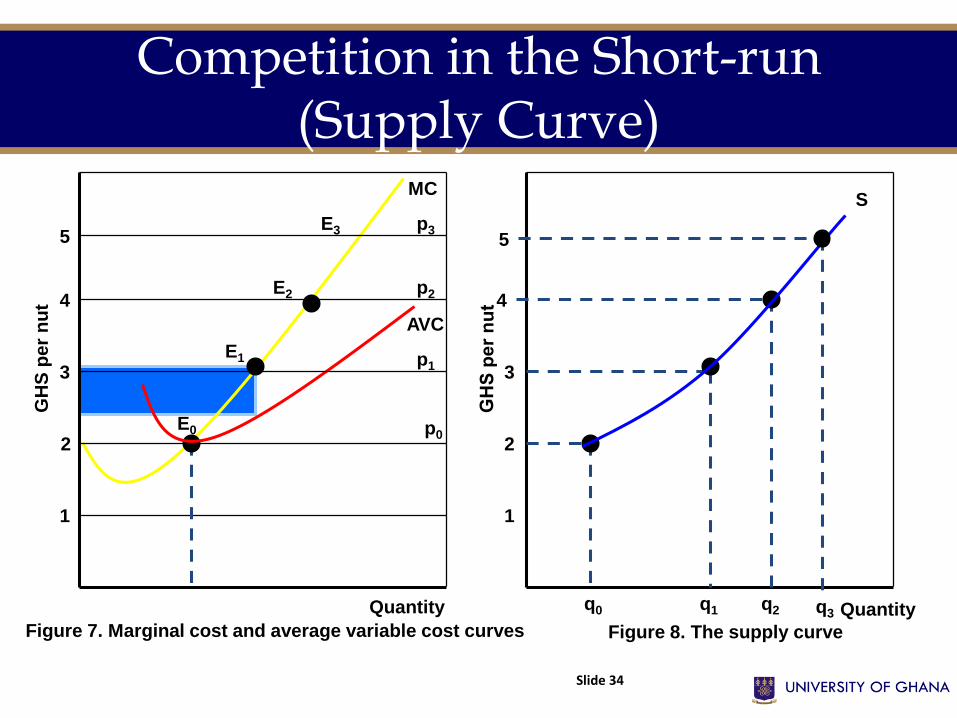
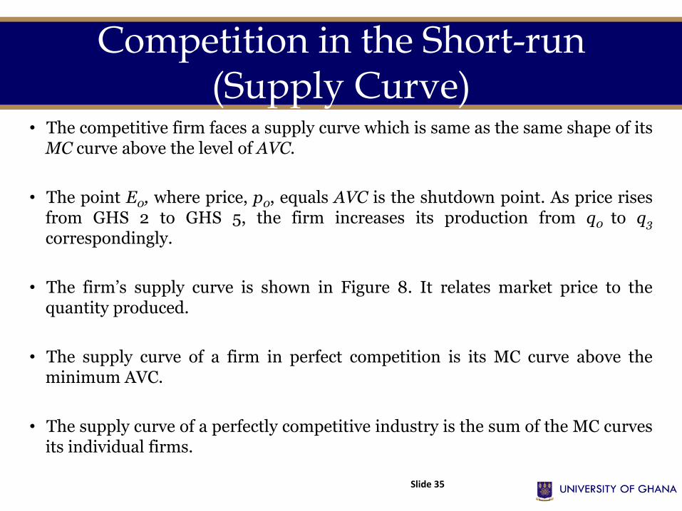
• The competitive firm faces a supply curve which is same as the same shape of itsMC curve above the level of AVC.

• The point E0, where price, p0, equals AVC is the shutdown point. As price risesfrom GHS 2 to GHS 5, the firm increases its production from q0 to q3

correspondingly.

• The firm’s supply curve is shown in Figure 8. It relates market price to thequantity produced.

• The supply curve of a firm in perfect competition is its MC curve above theminimum AVC.

• The supply curve of a perfectly competitive industry is the sum of the MC curvesits individual firms.

Slide 35


• The market supply curve is derived on the assumption that factor prices and technology are given and that there is a large number of firms in the market.

• Thus the total market output at each price is the sum of the outputs supplied by all firms at the prevailing price.

• The shape of the market supply curve is dependent on:

– Technology;

– Factor prices and

– Size distribution of firms in the market. Note that the firms are not of the same sizes as there are different entrepreneurial efficiencies.

• These factors will determine the shape of the market supply because they determine the cost structure of the firms in the market and thus by extension determine the shape of the industry supply curve.

Slide 36

Competition in the Short-run (Industry/Market Equilibrium)

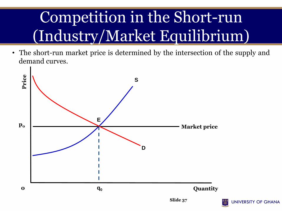
• The short-run market price is determined by the intersection of the supply anddemand curves.

Slide 37

Market pricep0

0 Quantity

Pr

ice

S

E

D

q0

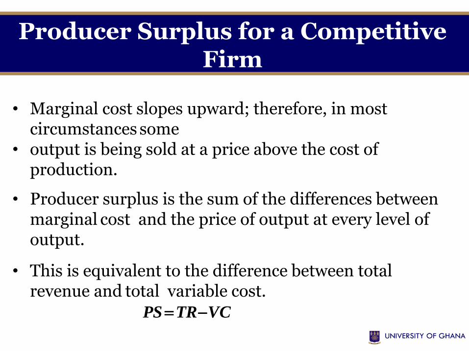
Producer Surplus for a CompetitiveFirm

• Marginal cost slopes upward; therefore, in most circumstances some

• output is being sold at a price above the cost ofproduction.

• Producer surplus is the sum of the differences between marginal cost and the price of output at every level ofoutput.

• This is equivalent to the difference between total revenue and total variable cost.

PSTRVC

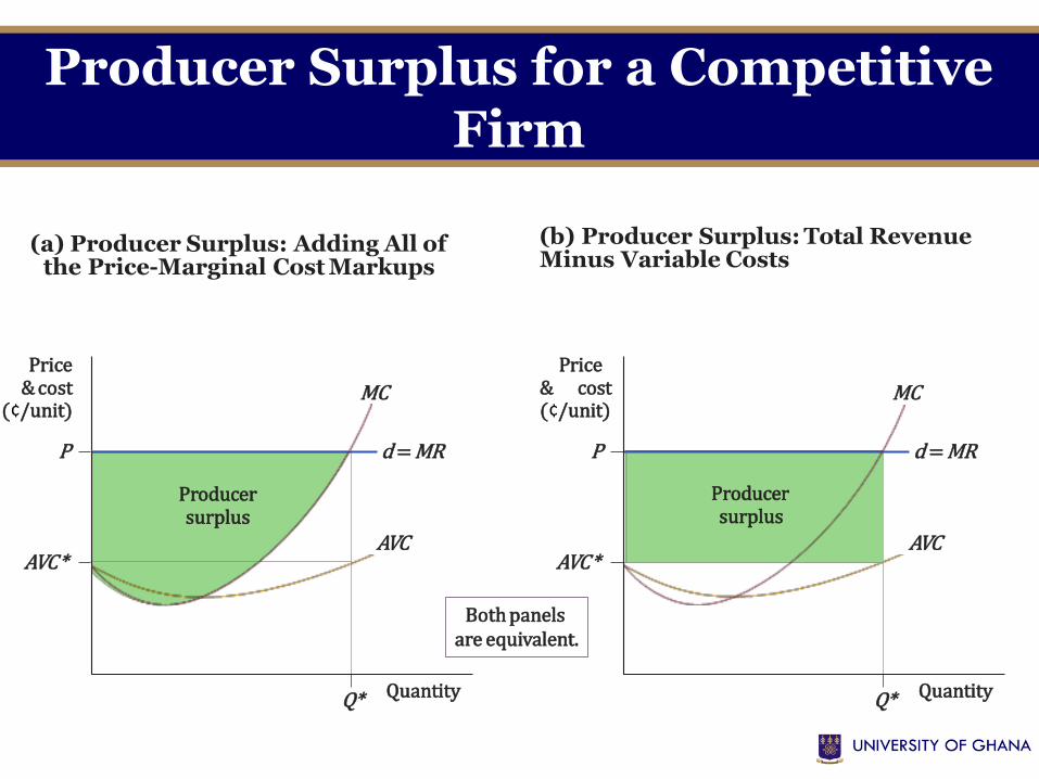
MC MC

Price & cost

(¢/unit)

Price& cost(¢/unit)

P d = MR P d = MR

Producer surplus

Producersurplus

AVC AVCAVC* AVC*

Quantity QuantityQ* Q*

Both panelsare equivalent.

(a) Producer Surplus: Adding All ofthe Price-Marginal Cost Markups

(b) Producer Surplus: Total RevenueMinus Variable Costs


Producer Surplus and Profit

• Producer surplus is closely related to profit, but they are not the same thing.

PS TRVC,

TRVCFC PSFC

• Firms will operate without making a profit, but they will shut down if they are not making any producersurplus.


Perfect Competition in the Short Run 8.3

Producer Surplus for a Competitive Industry

Producer surplus for an entire industry is the sum of individual firms’

surplus.

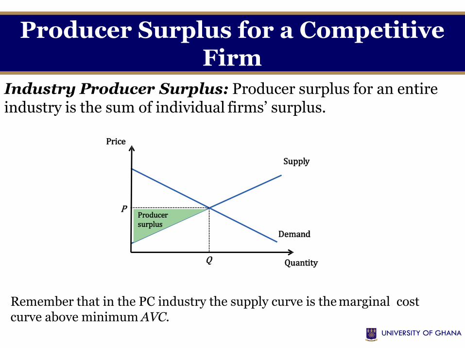
Industry Producer Surplus: Producer surplus for an entire industry is the sum of individual firms’ surplus.

Remember that in the PC industry the supply curve is the marginal cost curve above minimum AVC.

Quantity

Demand

Price

Supply

PProducer surplus

Q


Session Questions

• What defines a perfectly competitive market?

• Graphically distinguish between economic profit, normal profit, and economic loss.

• Explain the competitive firm’s profit maximizing condition.

• With graphs and examples, illustrate how to derive the supply curve.

• Explain the short-run competitive equilibrium.

Slide 43

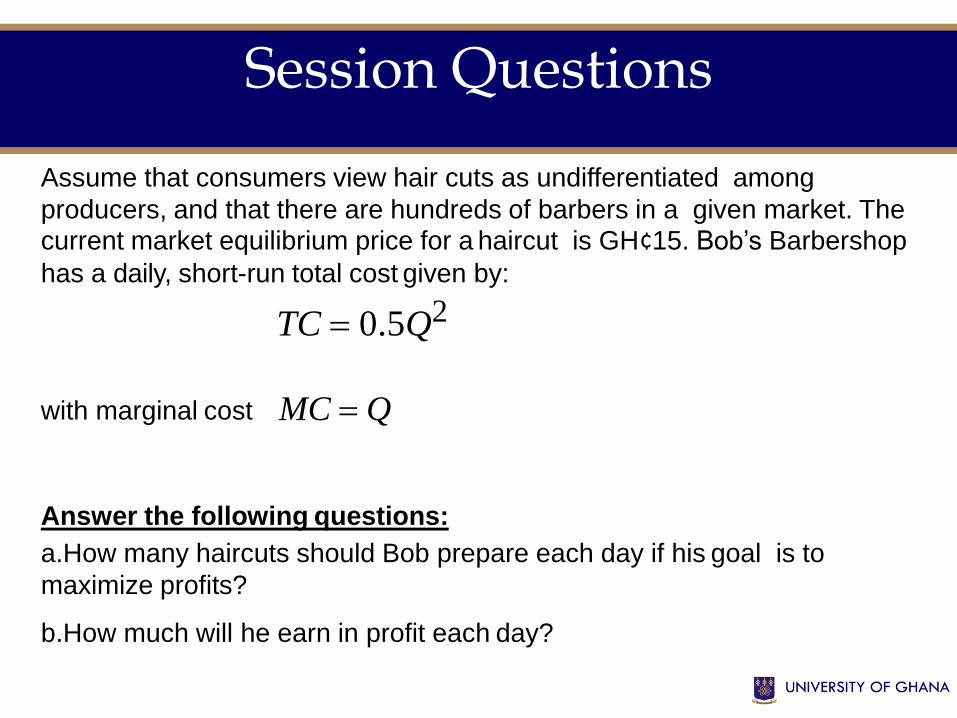
Assume that consumers view hair cuts as undifferentiated among

producers, and that there are hundreds of barbers in a given market. The current market equilibrium price for a haircut is GH¢15. Bob’s Barbershop

has a daily, short-run total cost given by:

with marginal cost

Answer the following questions:

a.How many haircuts should Bob prepare each day if his goal is to

maximize profits?

b.How much will he earn in profit each day?

TC 0.5Q2

MC Q

Session Questions

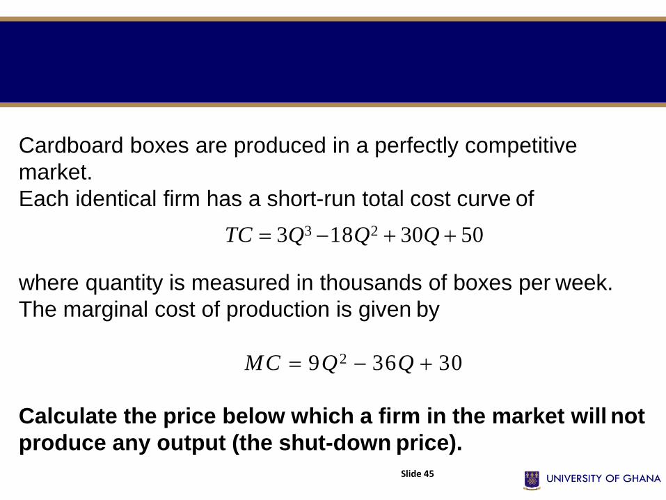
Cardboard boxes are produced in a perfectly competitive

market.

Each identical firm has a short-run total cost curve of

TC 3Q3 18Q2 30Q 50

where quantity is measured in thousands of boxes per week.

The marginal cost of production is given by

MC 9Q2 36Q 30

Calculate the price below which a firm in the market will not

produce any output (the shut-down price).

ECON 311 MICROECONOMICS THEORY I · ECON 311 MICROECONOMICS THEORY I ... profit by choosing the...

Documents

Transcript of ECON 311 MICROECONOMICS THEORY I · ECON 311 MICROECONOMICS THEORY I ... profit by choosing the...