Econ 101: Principles of Microeconomics · Econ 101: Principles of Microeconomics Chapter 12 -...
233
Econ 101: Principles of Microeconomics Chapter 12 - Behind the Supply Curve - Inputs and Costs Fall 2010 Herriges (ISU) Ch. 12 Behind the Supply Curve Fall 2010 1 / 30
-
Upload
vuongkhanh -
Category
Documents
-
view
242 -
download
0
Transcript of Econ 101: Principles of Microeconomics · Econ 101: Principles of Microeconomics Chapter 12 -...

Econ 101: Principles of MicroeconomicsChapter 12 - Behind the Supply Curve - Inputs and Costs
Fall 2010
Herriges (ISU) Ch. 12 Behind the Supply Curve Fall 2010 1 / 30

Outline
1 The Production Function
2 Marginal Cost and Average Cost
3 Short-Run versus Long-Run Costs
Herriges (ISU) Ch. 12 Behind the Supply Curve Fall 2010 2 / 30

Overview
In this chapter we turn our attention to the firm.
A firm is an organization that produces goods or services for sale.
We will begin by characterizing the relationship between the firm’sinputs and the quantity of outputs it produces.
The production function describes the relationship between thequantity of inputs and the quantity of outputs that the firm produces.
Basic characteristics of the production function has implications forthe cost structure for the firm, which in turn has implications for thefirm’ ultimate supply function.
Herriges (ISU) Ch. 12 Behind the Supply Curve Fall 2010 3 / 30
Overview
In this chapter we turn our attention to the firm.
A firm is an organization that produces goods or services for sale.
We will begin by characterizing the relationship between the firm’sinputs and the quantity of outputs it produces.
The production function describes the relationship between thequantity of inputs and the quantity of outputs that the firm produces.
Basic characteristics of the production function has implications forthe cost structure for the firm
, which in turn has implications for thefirm’ ultimate supply function.
Herriges (ISU) Ch. 12 Behind the Supply Curve Fall 2010 3 / 30

Overview
In this chapter we turn our attention to the firm.
A firm is an organization that produces goods or services for sale.
We will begin by characterizing the relationship between the firm’sinputs and the quantity of outputs it produces.
The production function describes the relationship between thequantity of inputs and the quantity of outputs that the firm produces.
Basic characteristics of the production function has implications forthe cost structure for the firm, which in turn has implications for thefirm’ ultimate supply function.
Herriges (ISU) Ch. 12 Behind the Supply Curve Fall 2010 3 / 30

The Production Function
The Short Run and the Long Run
It is useful to categorize firms’ decisions into
- Long-run decisions
–involves a time horizon long enough for a firm tovary all of its inputs
- Short-run decisions–involves any time horizon over which at least oneof the firm’s inputs cannot be varied
To guide the firm over the next several years, manager must use thelong-run view
To determine what the firm should do next week, the short run viewis best.
Herriges (ISU) Ch. 12 Behind the Supply Curve Fall 2010 4 / 30

The Production Function
The Short Run and the Long Run
It is useful to categorize firms’ decisions into
- Long-run decisions–involves a time horizon long enough for a firm tovary all of its inputs
- Short-run decisions
–involves any time horizon over which at least oneof the firm’s inputs cannot be varied
To guide the firm over the next several years, manager must use thelong-run view
To determine what the firm should do next week, the short run viewis best.
Herriges (ISU) Ch. 12 Behind the Supply Curve Fall 2010 4 / 30

The Production Function
The Short Run and the Long Run
It is useful to categorize firms’ decisions into
- Long-run decisions–involves a time horizon long enough for a firm tovary all of its inputs
- Short-run decisions–involves any time horizon over which at least oneof the firm’s inputs cannot be varied
To guide the firm over the next several years, manager must use thelong-run view
To determine what the firm should do next week, the short run viewis best.
Herriges (ISU) Ch. 12 Behind the Supply Curve Fall 2010 4 / 30

The Production Function
The Short Run and the Long Run
It is useful to categorize firms’ decisions into
- Long-run decisions–involves a time horizon long enough for a firm tovary all of its inputs
- Short-run decisions–involves any time horizon over which at least oneof the firm’s inputs cannot be varied
To guide the firm over the next several years, manager must use thelong-run view
To determine what the firm should do next week, the short run viewis best.
Herriges (ISU) Ch. 12 Behind the Supply Curve Fall 2010 4 / 30

The Production Function
Production in the Short Run
In the short-run, the firm’s inputs can be divided into one of twocategories
1 Fixed inputs
- These are inputs whose quantity is constant for some period of time(regardless of how much output is produced).
- Typically, fixed inputs will include land and machinery, though they canalso include certain types of labor (due to contracts).
2 Variable inputs
- These are inputs whose quantity the firm can vary, even in the shortrun.
- Examples of variable inputs often include labor, energy, fuel, etc.
When firms make short-run decisions, there is nothing they can doabout their fixed inputs; i.e., they are stuck with whatever quantitythey have.
However, they can make choices about their variable inputs.
Herriges (ISU) Ch. 12 Behind the Supply Curve Fall 2010 5 / 30

The Production Function
Total Product
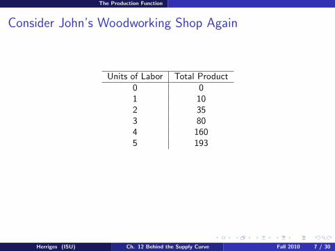
To fix ideas, suppose we have a firm whose only variable input is labor
All other inputs (capital, land, raw materials, etc.) we will assume fornow are fixed.
Total product is the maximum quantity of output that can beproduced from a given combination of inputs.
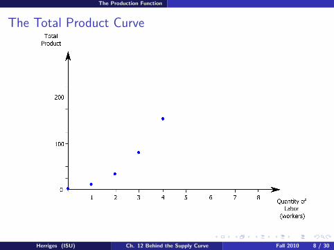
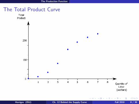
The total product curve shows how the quantity of output depends onthe quantity of variable input, for a given quantity of the fixed input.
We would generally expect the total product curve to be increasing;i.e., as the quantity of the variable input increases, we would expecttotal output to increase.
Herriges (ISU) Ch. 12 Behind the Supply Curve Fall 2010 6 / 30

The Production Function
Total Product
To fix ideas, suppose we have a firm whose only variable input is labor
All other inputs (capital, land, raw materials, etc.) we will assume fornow are fixed.
Total product is the maximum quantity of output that can beproduced from a given combination of inputs.
The total product curve shows how the quantity of output depends onthe quantity of variable input, for a given quantity of the fixed input.
We would generally expect the total product curve to be increasing;i.e., as the quantity of the variable input increases, we would expecttotal output to increase.
Herriges (ISU) Ch. 12 Behind the Supply Curve Fall 2010 6 / 30

The Production Function
Total Product
To fix ideas, suppose we have a firm whose only variable input is labor
All other inputs (capital, land, raw materials, etc.) we will assume fornow are fixed.
Total product is the maximum quantity of output that can beproduced from a given combination of inputs.
The total product curve shows how the quantity of output depends onthe quantity of variable input, for a given quantity of the fixed input.
We would generally expect the total product curve to be increasing
;i.e., as the quantity of the variable input increases, we would expecttotal output to increase.
Herriges (ISU) Ch. 12 Behind the Supply Curve Fall 2010 6 / 30

The Production Function
Total Product
To fix ideas, suppose we have a firm whose only variable input is labor
All other inputs (capital, land, raw materials, etc.) we will assume fornow are fixed.
Total product is the maximum quantity of output that can beproduced from a given combination of inputs.
The total product curve shows how the quantity of output depends onthe quantity of variable input, for a given quantity of the fixed input.
We would generally expect the total product curve to be increasing;i.e., as the quantity of the variable input increases, we would expecttotal output to increase.
Herriges (ISU) Ch. 12 Behind the Supply Curve Fall 2010 6 / 30

The Production Function
Consider John’s Woodworking Shop Again
Units of Labor Total Product0 0
1 102 353 804 1605 1936 2187 2398 257
Herriges (ISU) Ch. 12 Behind the Supply Curve Fall 2010 7 / 30

The Production Function
Consider John’s Woodworking Shop Again
Units of Labor Total Product0 01 10
2 353 804 1605 1936 2187 2398 257
Herriges (ISU) Ch. 12 Behind the Supply Curve Fall 2010 7 / 30

The Production Function
Consider John’s Woodworking Shop Again
Units of Labor Total Product0 01 102 35
3 804 1605 1936 2187 2398 257
Herriges (ISU) Ch. 12 Behind the Supply Curve Fall 2010 7 / 30

The Production Function
Consider John’s Woodworking Shop Again
Units of Labor Total Product0 01 102 353 80
4 1605 1936 2187 2398 257
Herriges (ISU) Ch. 12 Behind the Supply Curve Fall 2010 7 / 30

The Production Function
Consider John’s Woodworking Shop Again
Units of Labor Total Product0 01 102 353 804 160
5 1936 2187 2398 257
Herriges (ISU) Ch. 12 Behind the Supply Curve Fall 2010 7 / 30
The Production Function
Consider John’s Woodworking Shop Again
Units of Labor Total Product0 01 102 353 804 1605 193
6 2187 2398 257
Herriges (ISU) Ch. 12 Behind the Supply Curve Fall 2010 7 / 30

The Production Function
Consider John’s Woodworking Shop Again
Units of Labor Total Product0 01 102 353 804 1605 1936 218
7 2398 257
Herriges (ISU) Ch. 12 Behind the Supply Curve Fall 2010 7 / 30

The Production Function
Consider John’s Woodworking Shop Again
Units of Labor Total Product0 01 102 353 804 1605 1936 2187 239
8 257
Herriges (ISU) Ch. 12 Behind the Supply Curve Fall 2010 7 / 30

The Production Function
Consider John’s Woodworking Shop Again
Units of Labor Total Product0 01 102 353 804 1605 1936 2187 2398 257
Herriges (ISU) Ch. 12 Behind the Supply Curve Fall 2010 7 / 30

The Production Function
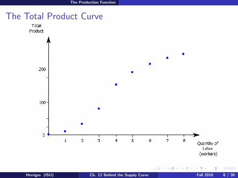
The Total Product Curve
Herriges (ISU) Ch. 12 Behind the Supply Curve Fall 2010 8 / 30

The Production Function
The Total Product Curve
Herriges (ISU) Ch. 12 Behind the Supply Curve Fall 2010 8 / 30

The Production Function
The Total Product Curve
Herriges (ISU) Ch. 12 Behind the Supply Curve Fall 2010 8 / 30

The Production Function
The Total Product Curve
Herriges (ISU) Ch. 12 Behind the Supply Curve Fall 2010 8 / 30
The Production Function
The Total Product Curve
Herriges (ISU) Ch. 12 Behind the Supply Curve Fall 2010 8 / 30

The Production Function
The Total Product Curve
Herriges (ISU) Ch. 12 Behind the Supply Curve Fall 2010 8 / 30

The Production Function
The Total Product Curve
Herriges (ISU) Ch. 12 Behind the Supply Curve Fall 2010 8 / 30
The Production Function
The Total Product Curve
Herriges (ISU) Ch. 12 Behind the Supply Curve Fall 2010 8 / 30
The Production Function
The Total Product Curve
Herriges (ISU) Ch. 12 Behind the Supply Curve Fall 2010 8 / 30

The Production Function
The Total Product Curve
Herriges (ISU) Ch. 12 Behind the Supply Curve Fall 2010 8 / 30
The Production Function
Marginal Product
Notice that the Total Product curve is always increasing in this case,but that it’s slope is not the same throughout.
- Initial the slope is increasing- but eventually it starts to flatten out.
The slope of the Total Product Curve is the Marginal Product oflabor.
Formally,
Marginal Product of Labor (MPL) =Change in Quantity of Output
Change in Quantity of Labor
=∆Q
∆L
Tells us the rise in output produced when one more worker is hired
Herriges (ISU) Ch. 12 Behind the Supply Curve Fall 2010 9 / 30

The Production Function
Marginal Product
Notice that the Total Product curve is always increasing in this case,but that it’s slope is not the same throughout.
- Initial the slope is increasing
- but eventually it starts to flatten out.
The slope of the Total Product Curve is the Marginal Product oflabor.
Formally,
Marginal Product of Labor (MPL) =Change in Quantity of Output
Change in Quantity of Labor
=∆Q
∆L
Tells us the rise in output produced when one more worker is hired
Herriges (ISU) Ch. 12 Behind the Supply Curve Fall 2010 9 / 30

The Production Function
Marginal Product
Notice that the Total Product curve is always increasing in this case,but that it’s slope is not the same throughout.
- Initial the slope is increasing- but eventually it starts to flatten out.
The slope of the Total Product Curve is the Marginal Product oflabor.
Formally,
Marginal Product of Labor (MPL) =Change in Quantity of Output
Change in Quantity of Labor
=∆Q
∆L
Tells us the rise in output produced when one more worker is hired
Herriges (ISU) Ch. 12 Behind the Supply Curve Fall 2010 9 / 30

The Production Function
Marginal Product
Notice that the Total Product curve is always increasing in this case,but that it’s slope is not the same throughout.
- Initial the slope is increasing- but eventually it starts to flatten out.
The slope of the Total Product Curve is the Marginal Product oflabor.
Formally,
Marginal Product of Labor (MPL) =Change in Quantity of Output
Change in Quantity of Labor
=∆Q
∆L
Tells us the rise in output produced when one more worker is hired
Herriges (ISU) Ch. 12 Behind the Supply Curve Fall 2010 9 / 30

The Production Function
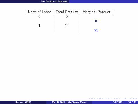
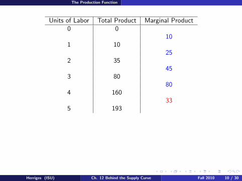
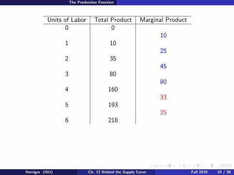
Units of Labor Total Product Marginal Product0 0
101 10
252 35
453 80
804 160
335 193
256 218
217 239
188 257
Herriges (ISU) Ch. 12 Behind the Supply Curve Fall 2010 10 / 30

The Production Function
Units of Labor Total Product Marginal Product0 0
10
1 1025
2 3545
3 8080
4 16033
5 19325
6 21821
7 23918
8 257
Herriges (ISU) Ch. 12 Behind the Supply Curve Fall 2010 10 / 30

The Production Function
Units of Labor Total Product Marginal Product0 0
101 10
252 35
453 80
804 160
335 193
256 218
217 239
188 257
Herriges (ISU) Ch. 12 Behind the Supply Curve Fall 2010 10 / 30
The Production Function
Units of Labor Total Product Marginal Product0 0
101 10
25
2 3545
3 8080
4 16033
5 19325
6 21821
7 23918
8 257
Herriges (ISU) Ch. 12 Behind the Supply Curve Fall 2010 10 / 30

The Production Function
Units of Labor Total Product Marginal Product0 0
101 10
252 35
453 80
804 160
335 193
256 218
217 239
188 257
Herriges (ISU) Ch. 12 Behind the Supply Curve Fall 2010 10 / 30

The Production Function
Units of Labor Total Product Marginal Product0 0
101 10
252 35
45
3 8080
4 16033
5 19325
6 21821
7 23918
8 257
Herriges (ISU) Ch. 12 Behind the Supply Curve Fall 2010 10 / 30

The Production Function
Units of Labor Total Product Marginal Product0 0
101 10
252 35
453 80
804 160
335 193
256 218
217 239
188 257
Herriges (ISU) Ch. 12 Behind the Supply Curve Fall 2010 10 / 30

The Production Function
Units of Labor Total Product Marginal Product0 0
101 10
252 35
453 80
80
4 16033
5 19325
6 21821
7 23918
8 257
Herriges (ISU) Ch. 12 Behind the Supply Curve Fall 2010 10 / 30

The Production Function
Units of Labor Total Product Marginal Product0 0
101 10
252 35
453 80
804 160
335 193
256 218
217 239
188 257
Herriges (ISU) Ch. 12 Behind the Supply Curve Fall 2010 10 / 30

The Production Function
Units of Labor Total Product Marginal Product0 0
101 10
252 35
453 80
804 160
33
5 19325
6 21821
7 23918
8 257
Herriges (ISU) Ch. 12 Behind the Supply Curve Fall 2010 10 / 30
The Production Function
Units of Labor Total Product Marginal Product0 0
101 10
252 35
453 80
804 160
335 193
256 218
217 239
188 257
Herriges (ISU) Ch. 12 Behind the Supply Curve Fall 2010 10 / 30

The Production Function
Units of Labor Total Product Marginal Product0 0
101 10
252 35
453 80
804 160
335 193
25
6 21821
7 23918
8 257
Herriges (ISU) Ch. 12 Behind the Supply Curve Fall 2010 10 / 30
The Production Function
Units of Labor Total Product Marginal Product0 0
101 10
252 35
453 80
804 160
335 193
256 218
217 239
188 257
Herriges (ISU) Ch. 12 Behind the Supply Curve Fall 2010 10 / 30

The Production Function
Units of Labor Total Product Marginal Product0 0
101 10
252 35
453 80
804 160
335 193
256 218
21
7 23918
8 257
Herriges (ISU) Ch. 12 Behind the Supply Curve Fall 2010 10 / 30

The Production Function
Units of Labor Total Product Marginal Product0 0
101 10
252 35
453 80
804 160
335 193
256 218
217 239
188 257
Herriges (ISU) Ch. 12 Behind the Supply Curve Fall 2010 10 / 30

The Production Function
Units of Labor Total Product Marginal Product0 0
101 10
252 35
453 80
804 160
335 193
256 218
217 239
18
8 257
Herriges (ISU) Ch. 12 Behind the Supply Curve Fall 2010 10 / 30

The Production Function
Units of Labor Total Product Marginal Product0 0
101 10
252 35
453 80
804 160
335 193
256 218
217 239
188 257
Herriges (ISU) Ch. 12 Behind the Supply Curve Fall 2010 10 / 30

The Production Function
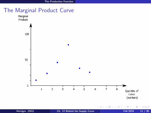
The Marginal Product Curve
Herriges (ISU) Ch. 12 Behind the Supply Curve Fall 2010 11 / 30

The Production Function
The Marginal Product Curve
Herriges (ISU) Ch. 12 Behind the Supply Curve Fall 2010 11 / 30

The Production Function
The Marginal Product Curve
Herriges (ISU) Ch. 12 Behind the Supply Curve Fall 2010 11 / 30

The Production Function
The Marginal Product Curve
Herriges (ISU) Ch. 12 Behind the Supply Curve Fall 2010 11 / 30

The Production Function
The Marginal Product Curve
Herriges (ISU) Ch. 12 Behind the Supply Curve Fall 2010 11 / 30
The Production Function
The Marginal Product Curve
Herriges (ISU) Ch. 12 Behind the Supply Curve Fall 2010 11 / 30

The Production Function
The Marginal Product Curve
Herriges (ISU) Ch. 12 Behind the Supply Curve Fall 2010 11 / 30

The Production Function
The Marginal Product Curve
Herriges (ISU) Ch. 12 Behind the Supply Curve Fall 2010 11 / 30

The Production Function
The Marginal Product Curve
Herriges (ISU) Ch. 12 Behind the Supply Curve Fall 2010 11 / 30

The Production Function
Marginal Returns To Labor
As more and more workers are hired, the MPL is at first increasing
- This is known as increasing returns to labor- This is typically due to the returns to specialization- It can also arise due to minimum labor requirements for equipment.
Eventually, however, the MPL starts to decline
- This is known as diminishing returns to labor- This arises as the gains from specialization are exhausted and- The constraints caused by the fixed inputs start to bind
This pattern of MPL (and for other inputs) is thought to hold formost industries.
Consider the problem of a woodworking shop.
Herriges (ISU) Ch. 12 Behind the Supply Curve Fall 2010 12 / 30

The Production Function
Marginal Returns To Labor
As more and more workers are hired, the MPL is at first increasing
- This is known as increasing returns to labor
- This is typically due to the returns to specialization- It can also arise due to minimum labor requirements for equipment.
Eventually, however, the MPL starts to decline
- This is known as diminishing returns to labor- This arises as the gains from specialization are exhausted and- The constraints caused by the fixed inputs start to bind
This pattern of MPL (and for other inputs) is thought to hold formost industries.
Consider the problem of a woodworking shop.
Herriges (ISU) Ch. 12 Behind the Supply Curve Fall 2010 12 / 30
The Production Function
Marginal Returns To Labor
As more and more workers are hired, the MPL is at first increasing
- This is known as increasing returns to labor- This is typically due to the returns to specialization
- It can also arise due to minimum labor requirements for equipment.
Eventually, however, the MPL starts to decline
- This is known as diminishing returns to labor- This arises as the gains from specialization are exhausted and- The constraints caused by the fixed inputs start to bind
This pattern of MPL (and for other inputs) is thought to hold formost industries.
Consider the problem of a woodworking shop.
Herriges (ISU) Ch. 12 Behind the Supply Curve Fall 2010 12 / 30

The Production Function
Marginal Returns To Labor
As more and more workers are hired, the MPL is at first increasing
- This is known as increasing returns to labor- This is typically due to the returns to specialization- It can also arise due to minimum labor requirements for equipment.
Eventually, however, the MPL starts to decline
- This is known as diminishing returns to labor- This arises as the gains from specialization are exhausted and- The constraints caused by the fixed inputs start to bind
This pattern of MPL (and for other inputs) is thought to hold formost industries.
Consider the problem of a woodworking shop.
Herriges (ISU) Ch. 12 Behind the Supply Curve Fall 2010 12 / 30

The Production Function
Marginal Returns To Labor
As more and more workers are hired, the MPL is at first increasing
- This is known as increasing returns to labor- This is typically due to the returns to specialization- It can also arise due to minimum labor requirements for equipment.
Eventually, however, the MPL starts to decline
- This is known as diminishing returns to labor
- This arises as the gains from specialization are exhausted and- The constraints caused by the fixed inputs start to bind
This pattern of MPL (and for other inputs) is thought to hold formost industries.
Consider the problem of a woodworking shop.
Herriges (ISU) Ch. 12 Behind the Supply Curve Fall 2010 12 / 30

The Production Function
Marginal Returns To Labor
As more and more workers are hired, the MPL is at first increasing
- This is known as increasing returns to labor- This is typically due to the returns to specialization- It can also arise due to minimum labor requirements for equipment.
Eventually, however, the MPL starts to decline
- This is known as diminishing returns to labor- This arises as the gains from specialization are exhausted and
- The constraints caused by the fixed inputs start to bind
This pattern of MPL (and for other inputs) is thought to hold formost industries.
Consider the problem of a woodworking shop.
Herriges (ISU) Ch. 12 Behind the Supply Curve Fall 2010 12 / 30
The Production Function
Marginal Returns To Labor
As more and more workers are hired, the MPL is at first increasing
- This is known as increasing returns to labor- This is typically due to the returns to specialization- It can also arise due to minimum labor requirements for equipment.
Eventually, however, the MPL starts to decline
- This is known as diminishing returns to labor- This arises as the gains from specialization are exhausted and- The constraints caused by the fixed inputs start to bind
This pattern of MPL (and for other inputs) is thought to hold formost industries.
Consider the problem of a woodworking shop.
Herriges (ISU) Ch. 12 Behind the Supply Curve Fall 2010 12 / 30

The Production Function
Marginal Returns To Labor
As more and more workers are hired, the MPL is at first increasing
- This is known as increasing returns to labor- This is typically due to the returns to specialization- It can also arise due to minimum labor requirements for equipment.
Eventually, however, the MPL starts to decline
- This is known as diminishing returns to labor- This arises as the gains from specialization are exhausted and- The constraints caused by the fixed inputs start to bind
This pattern of MPL (and for other inputs) is thought to hold formost industries.
Consider the problem of a woodworking shop.
Herriges (ISU) Ch. 12 Behind the Supply Curve Fall 2010 12 / 30

Marginal Cost and Average Cost
Production and Firm Costs
Understanding the nature of a firm’s production function is importantin that it has implications for the firm’s costs.
In the short run, the firm’s costs can be divided into two broadcategories:
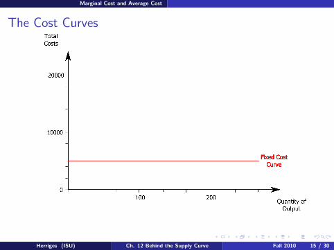
1 Total Fixed costs (TFC): These are costs that do not depend upon thequantity of output produced.
- These costs are typically associated with fixed inputs.- Examples of fixed costs might be the rent paid for the firm’s building or
equipment rentals.
2 Total Variable costs (TVC): These are costs that depend on thequantity output produced.
- As the name suggests, these are costs associated with the variableinputs.
- In the case of John’s Woodworking shop, the TVC = w × L where wdenotes the wage rate.
Total Costs = TFC + TVC.
Herriges (ISU) Ch. 12 Behind the Supply Curve Fall 2010 13 / 30

Marginal Cost and Average Cost
Production and Firm Costs
Understanding the nature of a firm’s production function is importantin that it has implications for the firm’s costs.
In the short run, the firm’s costs can be divided into two broadcategories:
1 Total Fixed costs (TFC): These are costs that do not depend upon thequantity of output produced.
- These costs are typically associated with fixed inputs.
- Examples of fixed costs might be the rent paid for the firm’s building orequipment rentals.
2 Total Variable costs (TVC): These are costs that depend on thequantity output produced.
- As the name suggests, these are costs associated with the variableinputs.
- In the case of John’s Woodworking shop, the TVC = w × L where wdenotes the wage rate.
Total Costs = TFC + TVC.
Herriges (ISU) Ch. 12 Behind the Supply Curve Fall 2010 13 / 30

Marginal Cost and Average Cost
Production and Firm Costs
Understanding the nature of a firm’s production function is importantin that it has implications for the firm’s costs.
In the short run, the firm’s costs can be divided into two broadcategories:
1 Total Fixed costs (TFC): These are costs that do not depend upon thequantity of output produced.
- These costs are typically associated with fixed inputs.- Examples of fixed costs might be the rent paid for the firm’s building or
equipment rentals.
2 Total Variable costs (TVC): These are costs that depend on thequantity output produced.
- As the name suggests, these are costs associated with the variableinputs.
- In the case of John’s Woodworking shop, the TVC = w × L where wdenotes the wage rate.
Total Costs = TFC + TVC.
Herriges (ISU) Ch. 12 Behind the Supply Curve Fall 2010 13 / 30

Marginal Cost and Average Cost
Production and Firm Costs
Understanding the nature of a firm’s production function is importantin that it has implications for the firm’s costs.
In the short run, the firm’s costs can be divided into two broadcategories:
1 Total Fixed costs (TFC): These are costs that do not depend upon thequantity of output produced.
- These costs are typically associated with fixed inputs.- Examples of fixed costs might be the rent paid for the firm’s building or
equipment rentals.
2 Total Variable costs (TVC): These are costs that depend on thequantity output produced.
- As the name suggests, these are costs associated with the variableinputs.
- In the case of John’s Woodworking shop, the TVC = w × L where wdenotes the wage rate.
Total Costs = TFC + TVC.
Herriges (ISU) Ch. 12 Behind the Supply Curve Fall 2010 13 / 30

Marginal Cost and Average Cost
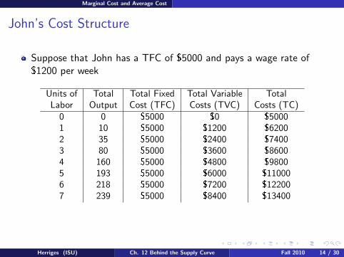
John’s Cost Structure
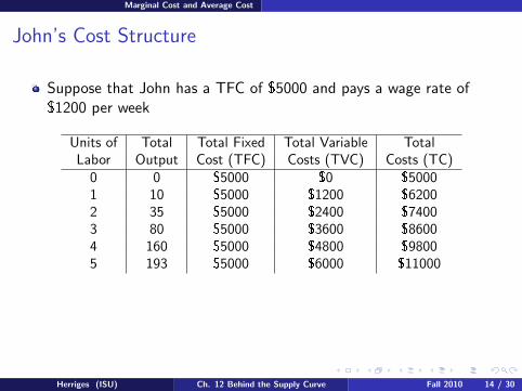
Suppose that John has a TFC of $5000 and pays a wage rate of$1200 per week
Units of Total Total Fixed Total Variable TotalLabor Output Cost (TFC) Costs (TVC) Costs (TC)
0 0 $5000 $0 $50001 10 $5000 $1200 $62002 35 $5000 $2400 $74003 80 $5000 $3600 $86004 160 $5000 $4800 $98005 193 $5000 $6000 $110006 218 $5000 $7200 $122007 239 $5000 $8400 $134008 257 $5000 $9600 $14600
Herriges (ISU) Ch. 12 Behind the Supply Curve Fall 2010 14 / 30

Marginal Cost and Average Cost
John’s Cost Structure
Suppose that John has a TFC of $5000 and pays a wage rate of$1200 per week
Units of Total Total Fixed Total Variable TotalLabor Output Cost (TFC) Costs (TVC) Costs (TC)
0 0 $5000 $0 $5000
1 10 $5000 $1200 $62002 35 $5000 $2400 $74003 80 $5000 $3600 $86004 160 $5000 $4800 $98005 193 $5000 $6000 $110006 218 $5000 $7200 $122007 239 $5000 $8400 $134008 257 $5000 $9600 $14600
Herriges (ISU) Ch. 12 Behind the Supply Curve Fall 2010 14 / 30

Marginal Cost and Average Cost
John’s Cost Structure
Suppose that John has a TFC of $5000 and pays a wage rate of$1200 per week
Units of Total Total Fixed Total Variable TotalLabor Output Cost (TFC) Costs (TVC) Costs (TC)
0 0 $5000 $0 $50001 10 $5000 $1200 $6200
2 35 $5000 $2400 $74003 80 $5000 $3600 $86004 160 $5000 $4800 $98005 193 $5000 $6000 $110006 218 $5000 $7200 $122007 239 $5000 $8400 $134008 257 $5000 $9600 $14600
Herriges (ISU) Ch. 12 Behind the Supply Curve Fall 2010 14 / 30

Marginal Cost and Average Cost
John’s Cost Structure
Suppose that John has a TFC of $5000 and pays a wage rate of$1200 per week
Units of Total Total Fixed Total Variable TotalLabor Output Cost (TFC) Costs (TVC) Costs (TC)
0 0 $5000 $0 $50001 10 $5000 $1200 $62002 35 $5000 $2400 $7400
3 80 $5000 $3600 $86004 160 $5000 $4800 $98005 193 $5000 $6000 $110006 218 $5000 $7200 $122007 239 $5000 $8400 $134008 257 $5000 $9600 $14600
Herriges (ISU) Ch. 12 Behind the Supply Curve Fall 2010 14 / 30

Marginal Cost and Average Cost
John’s Cost Structure
Suppose that John has a TFC of $5000 and pays a wage rate of$1200 per week
Units of Total Total Fixed Total Variable TotalLabor Output Cost (TFC) Costs (TVC) Costs (TC)
0 0 $5000 $0 $50001 10 $5000 $1200 $62002 35 $5000 $2400 $74003 80 $5000 $3600 $8600
4 160 $5000 $4800 $98005 193 $5000 $6000 $110006 218 $5000 $7200 $122007 239 $5000 $8400 $134008 257 $5000 $9600 $14600
Herriges (ISU) Ch. 12 Behind the Supply Curve Fall 2010 14 / 30

Marginal Cost and Average Cost
John’s Cost Structure
Suppose that John has a TFC of $5000 and pays a wage rate of$1200 per week
Units of Total Total Fixed Total Variable TotalLabor Output Cost (TFC) Costs (TVC) Costs (TC)
0 0 $5000 $0 $50001 10 $5000 $1200 $62002 35 $5000 $2400 $74003 80 $5000 $3600 $86004 160 $5000 $4800 $9800
5 193 $5000 $6000 $110006 218 $5000 $7200 $122007 239 $5000 $8400 $134008 257 $5000 $9600 $14600
Herriges (ISU) Ch. 12 Behind the Supply Curve Fall 2010 14 / 30
Marginal Cost and Average Cost
John’s Cost Structure
Suppose that John has a TFC of $5000 and pays a wage rate of$1200 per week
Units of Total Total Fixed Total Variable TotalLabor Output Cost (TFC) Costs (TVC) Costs (TC)
0 0 $5000 $0 $50001 10 $5000 $1200 $62002 35 $5000 $2400 $74003 80 $5000 $3600 $86004 160 $5000 $4800 $98005 193 $5000 $6000 $11000
6 218 $5000 $7200 $122007 239 $5000 $8400 $134008 257 $5000 $9600 $14600
Herriges (ISU) Ch. 12 Behind the Supply Curve Fall 2010 14 / 30

Marginal Cost and Average Cost
John’s Cost Structure
Suppose that John has a TFC of $5000 and pays a wage rate of$1200 per week
Units of Total Total Fixed Total Variable TotalLabor Output Cost (TFC) Costs (TVC) Costs (TC)
0 0 $5000 $0 $50001 10 $5000 $1200 $62002 35 $5000 $2400 $74003 80 $5000 $3600 $86004 160 $5000 $4800 $98005 193 $5000 $6000 $110006 218 $5000 $7200 $12200
7 239 $5000 $8400 $134008 257 $5000 $9600 $14600
Herriges (ISU) Ch. 12 Behind the Supply Curve Fall 2010 14 / 30
Marginal Cost and Average Cost
John’s Cost Structure
Suppose that John has a TFC of $5000 and pays a wage rate of$1200 per week
Units of Total Total Fixed Total Variable TotalLabor Output Cost (TFC) Costs (TVC) Costs (TC)
0 0 $5000 $0 $50001 10 $5000 $1200 $62002 35 $5000 $2400 $74003 80 $5000 $3600 $86004 160 $5000 $4800 $98005 193 $5000 $6000 $110006 218 $5000 $7200 $122007 239 $5000 $8400 $13400
8 257 $5000 $9600 $14600
Herriges (ISU) Ch. 12 Behind the Supply Curve Fall 2010 14 / 30

Marginal Cost and Average Cost
John’s Cost Structure
Suppose that John has a TFC of $5000 and pays a wage rate of$1200 per week
Units of Total Total Fixed Total Variable TotalLabor Output Cost (TFC) Costs (TVC) Costs (TC)
0 0 $5000 $0 $50001 10 $5000 $1200 $62002 35 $5000 $2400 $74003 80 $5000 $3600 $86004 160 $5000 $4800 $98005 193 $5000 $6000 $110006 218 $5000 $7200 $122007 239 $5000 $8400 $134008 257 $5000 $9600 $14600
Herriges (ISU) Ch. 12 Behind the Supply Curve Fall 2010 14 / 30
Marginal Cost and Average Cost
The Cost Curves
Herriges (ISU) Ch. 12 Behind the Supply Curve Fall 2010 15 / 30

Marginal Cost and Average Cost
The Cost Curves
Herriges (ISU) Ch. 12 Behind the Supply Curve Fall 2010 15 / 30

Marginal Cost and Average Cost
The Cost Curves
Herriges (ISU) Ch. 12 Behind the Supply Curve Fall 2010 15 / 30

Marginal Cost and Average Cost
The Cost Curves
Herriges (ISU) Ch. 12 Behind the Supply Curve Fall 2010 15 / 30

Marginal Cost and Average Cost
The Cost Curves
Herriges (ISU) Ch. 12 Behind the Supply Curve Fall 2010 15 / 30

Marginal Cost and Average Cost
The Cost Curves
Herriges (ISU) Ch. 12 Behind the Supply Curve Fall 2010 15 / 30

Marginal Cost and Average Cost
The Cost Curves
Herriges (ISU) Ch. 12 Behind the Supply Curve Fall 2010 15 / 30

Marginal Cost and Average Cost
The Cost Curves
Herriges (ISU) Ch. 12 Behind the Supply Curve Fall 2010 15 / 30

Marginal Cost and Average Cost
The Cost Curves
Herriges (ISU) Ch. 12 Behind the Supply Curve Fall 2010 15 / 30

Marginal Cost and Average Cost
The Cost Curves
Herriges (ISU) Ch. 12 Behind the Supply Curve Fall 2010 15 / 30

Marginal Cost and Average Cost
The Cost Curves
Herriges (ISU) Ch. 12 Behind the Supply Curve Fall 2010 15 / 30

Marginal Cost and Average Cost
The Cost Curves
Herriges (ISU) Ch. 12 Behind the Supply Curve Fall 2010 15 / 30

Marginal Cost and Average Cost
Marginal and Average Cost Curves
While the breakdown of Total Cost into Total Fixed and TotalVariable Costs is helpful, two other measures of cost will be evenmore useful:
1 Marginal Cost: Measures the additional cost of producing one moreunit of a good or service.
2 Average Cost: Measures the average cost per unit of the good orservice (i.e., the costs averaged over all of the output produced by thefirm).
Understanding the distinction between these two concepts will be keyto finding the optimal level of production for the firm.
We’ll start with average cost
Herriges (ISU) Ch. 12 Behind the Supply Curve Fall 2010 16 / 30

Marginal Cost and Average Cost
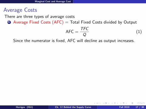
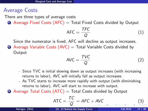
Average CostsThere are three types of average costs
1 Average Fixed Costs (AFC) = Total Fixed Costs divided by Output
AFC =TFC
Q(1)
Since the numerator is fixed, AFC will decline as output increases.2 Average Variable Costs (AVC) = Total Variable Costs divided by
Output
AVC =TVC
Q(2)
- Since TVC is initial slowing down as output increases (with increasingreturns to labor), AVC will initially fall as output increases.
- As TVC starts to increase more rapidly with output (with diminishingreturns to labor), AVC will start to increase with output.
3 Average Total Costs (ATC) = Total Costs divided by Output
ATC =TC
Q= AFC + AVC (3)
Herriges (ISU) Ch. 12 Behind the Supply Curve Fall 2010 17 / 30

Marginal Cost and Average Cost
Average CostsThere are three types of average costs
1 Average Fixed Costs (AFC) = Total Fixed Costs divided by Output
AFC =TFC
Q(1)
Since the numerator is fixed, AFC will decline as output increases.2 Average Variable Costs (AVC) = Total Variable Costs divided by
Output
AVC =TVC
Q(2)
- Since TVC is initial slowing down as output increases (with increasingreturns to labor), AVC will initially fall as output increases.
- As TVC starts to increase more rapidly with output (with diminishingreturns to labor), AVC will start to increase with output.
3 Average Total Costs (ATC) = Total Costs divided by Output
ATC =TC
Q= AFC + AVC (3)
Herriges (ISU) Ch. 12 Behind the Supply Curve Fall 2010 17 / 30
Marginal Cost and Average Cost
Average CostsThere are three types of average costs
1 Average Fixed Costs (AFC) = Total Fixed Costs divided by Output
AFC =TFC
Q(1)
Since the numerator is fixed, AFC will decline as output increases.
2 Average Variable Costs (AVC) = Total Variable Costs divided byOutput
AVC =TVC
Q(2)
- Since TVC is initial slowing down as output increases (with increasingreturns to labor), AVC will initially fall as output increases.
- As TVC starts to increase more rapidly with output (with diminishingreturns to labor), AVC will start to increase with output.
3 Average Total Costs (ATC) = Total Costs divided by Output
ATC =TC
Q= AFC + AVC (3)
Herriges (ISU) Ch. 12 Behind the Supply Curve Fall 2010 17 / 30

Marginal Cost and Average Cost
Average CostsThere are three types of average costs
1 Average Fixed Costs (AFC) = Total Fixed Costs divided by Output
AFC =TFC
Q(1)
Since the numerator is fixed, AFC will decline as output increases.2 Average Variable Costs (AVC) = Total Variable Costs divided by
Output
AVC =TVC
Q(2)
- Since TVC is initial slowing down as output increases (with increasingreturns to labor), AVC will initially fall as output increases.
- As TVC starts to increase more rapidly with output (with diminishingreturns to labor), AVC will start to increase with output.
3 Average Total Costs (ATC) = Total Costs divided by Output
ATC =TC
Q= AFC + AVC (3)
Herriges (ISU) Ch. 12 Behind the Supply Curve Fall 2010 17 / 30

Marginal Cost and Average Cost
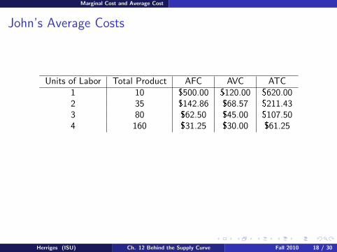
John’s Average Costs
Units of Labor Total Product AFC AVC ATC1 10 $500.00 $120.00 $620.00
2 35 $142.86 $68.57 $211.433 80 $62.50 $45.00 $107.504 160 $31.25 $30.00 $61.255 193 $25.91 $31.09 $56.996 218 $22.94 $33.03 $55.967 239 $20.92 $35.15 $56.078 257 $19.46 $37.35 $56.81
Herriges (ISU) Ch. 12 Behind the Supply Curve Fall 2010 18 / 30

Marginal Cost and Average Cost
John’s Average Costs
Units of Labor Total Product AFC AVC ATC1 10 $500.00 $120.00 $620.002 35 $142.86 $68.57 $211.43
3 80 $62.50 $45.00 $107.504 160 $31.25 $30.00 $61.255 193 $25.91 $31.09 $56.996 218 $22.94 $33.03 $55.967 239 $20.92 $35.15 $56.078 257 $19.46 $37.35 $56.81
Herriges (ISU) Ch. 12 Behind the Supply Curve Fall 2010 18 / 30

Marginal Cost and Average Cost
John’s Average Costs
Units of Labor Total Product AFC AVC ATC1 10 $500.00 $120.00 $620.002 35 $142.86 $68.57 $211.433 80 $62.50 $45.00 $107.50
4 160 $31.25 $30.00 $61.255 193 $25.91 $31.09 $56.996 218 $22.94 $33.03 $55.967 239 $20.92 $35.15 $56.078 257 $19.46 $37.35 $56.81
Herriges (ISU) Ch. 12 Behind the Supply Curve Fall 2010 18 / 30
Marginal Cost and Average Cost
John’s Average Costs
Units of Labor Total Product AFC AVC ATC1 10 $500.00 $120.00 $620.002 35 $142.86 $68.57 $211.433 80 $62.50 $45.00 $107.504 160 $31.25 $30.00 $61.25
5 193 $25.91 $31.09 $56.996 218 $22.94 $33.03 $55.967 239 $20.92 $35.15 $56.078 257 $19.46 $37.35 $56.81
Herriges (ISU) Ch. 12 Behind the Supply Curve Fall 2010 18 / 30

Marginal Cost and Average Cost
John’s Average Costs
Units of Labor Total Product AFC AVC ATC1 10 $500.00 $120.00 $620.002 35 $142.86 $68.57 $211.433 80 $62.50 $45.00 $107.504 160 $31.25 $30.00 $61.255 193 $25.91 $31.09 $56.99
6 218 $22.94 $33.03 $55.967 239 $20.92 $35.15 $56.078 257 $19.46 $37.35 $56.81
Herriges (ISU) Ch. 12 Behind the Supply Curve Fall 2010 18 / 30

Marginal Cost and Average Cost
John’s Average Costs
Units of Labor Total Product AFC AVC ATC1 10 $500.00 $120.00 $620.002 35 $142.86 $68.57 $211.433 80 $62.50 $45.00 $107.504 160 $31.25 $30.00 $61.255 193 $25.91 $31.09 $56.996 218 $22.94 $33.03 $55.96
7 239 $20.92 $35.15 $56.078 257 $19.46 $37.35 $56.81
Herriges (ISU) Ch. 12 Behind the Supply Curve Fall 2010 18 / 30

Marginal Cost and Average Cost
John’s Average Costs
Units of Labor Total Product AFC AVC ATC1 10 $500.00 $120.00 $620.002 35 $142.86 $68.57 $211.433 80 $62.50 $45.00 $107.504 160 $31.25 $30.00 $61.255 193 $25.91 $31.09 $56.996 218 $22.94 $33.03 $55.967 239 $20.92 $35.15 $56.07
8 257 $19.46 $37.35 $56.81
Herriges (ISU) Ch. 12 Behind the Supply Curve Fall 2010 18 / 30

Marginal Cost and Average Cost
John’s Average Costs
Units of Labor Total Product AFC AVC ATC1 10 $500.00 $120.00 $620.002 35 $142.86 $68.57 $211.433 80 $62.50 $45.00 $107.504 160 $31.25 $30.00 $61.255 193 $25.91 $31.09 $56.996 218 $22.94 $33.03 $55.967 239 $20.92 $35.15 $56.078 257 $19.46 $37.35 $56.81
Herriges (ISU) Ch. 12 Behind the Supply Curve Fall 2010 18 / 30

Marginal Cost and Average Cost
The Average Cost Curves
Herriges (ISU) Ch. 12 Behind the Supply Curve Fall 2010 19 / 30

Marginal Cost and Average Cost
The Average Cost Curves
Herriges (ISU) Ch. 12 Behind the Supply Curve Fall 2010 19 / 30

Marginal Cost and Average Cost
The Average Cost Curves
Herriges (ISU) Ch. 12 Behind the Supply Curve Fall 2010 19 / 30

Marginal Cost and Average Cost
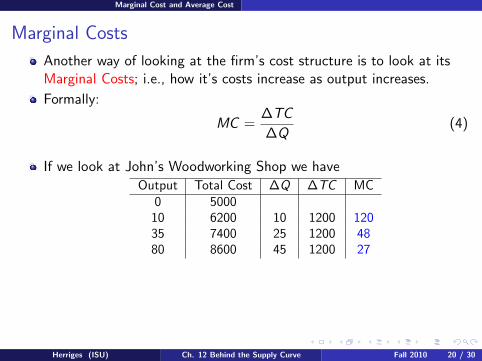
Marginal Costs
Another way of looking at the firm’s cost structure is to look at itsMarginal Costs; i.e., how it’s costs increase as output increases.
Formally:
MC =∆TC
∆Q(4)
If we look at John’s Woodworking Shop we have
Output Total Cost ∆Q ∆TC MC0 5000
10 6200 10 1200 12035 7400 25 1200 4880 8600 45 1200 27
160 9800 80 1200 15193 11000 33 1200 36218 12200 25 1200 48239 13400 21 1200 57257 14600 18 1200 67
Herriges (ISU) Ch. 12 Behind the Supply Curve Fall 2010 20 / 30

Marginal Cost and Average Cost
Marginal Costs
Another way of looking at the firm’s cost structure is to look at itsMarginal Costs; i.e., how it’s costs increase as output increases.
Formally:
MC =∆TC
∆Q(4)
If we look at John’s Woodworking Shop we have
Output Total Cost ∆Q ∆TC MC0 5000
10 6200 10 1200 120
35 7400 25 1200 4880 8600 45 1200 27
160 9800 80 1200 15193 11000 33 1200 36218 12200 25 1200 48239 13400 21 1200 57257 14600 18 1200 67
Herriges (ISU) Ch. 12 Behind the Supply Curve Fall 2010 20 / 30

Marginal Cost and Average Cost
Marginal Costs
Another way of looking at the firm’s cost structure is to look at itsMarginal Costs; i.e., how it’s costs increase as output increases.
Formally:
MC =∆TC
∆Q(4)
If we look at John’s Woodworking Shop we have
Output Total Cost ∆Q ∆TC MC0 5000
10 6200 10 1200 12035 7400 25 1200 48
80 8600 45 1200 27160 9800 80 1200 15193 11000 33 1200 36218 12200 25 1200 48239 13400 21 1200 57257 14600 18 1200 67
Herriges (ISU) Ch. 12 Behind the Supply Curve Fall 2010 20 / 30
Marginal Cost and Average Cost
Marginal Costs
Another way of looking at the firm’s cost structure is to look at itsMarginal Costs; i.e., how it’s costs increase as output increases.
Formally:
MC =∆TC
∆Q(4)
If we look at John’s Woodworking Shop we have
Output Total Cost ∆Q ∆TC MC0 5000
10 6200 10 1200 12035 7400 25 1200 4880 8600 45 1200 27
160 9800 80 1200 15193 11000 33 1200 36218 12200 25 1200 48239 13400 21 1200 57257 14600 18 1200 67
Herriges (ISU) Ch. 12 Behind the Supply Curve Fall 2010 20 / 30

Marginal Cost and Average Cost
Marginal Costs
Another way of looking at the firm’s cost structure is to look at itsMarginal Costs; i.e., how it’s costs increase as output increases.
Formally:
MC =∆TC
∆Q(4)
If we look at John’s Woodworking Shop we have
Output Total Cost ∆Q ∆TC MC0 5000
10 6200 10 1200 12035 7400 25 1200 4880 8600 45 1200 27
160 9800 80 1200 15
193 11000 33 1200 36218 12200 25 1200 48239 13400 21 1200 57257 14600 18 1200 67
Herriges (ISU) Ch. 12 Behind the Supply Curve Fall 2010 20 / 30

Marginal Cost and Average Cost
Marginal Costs
Another way of looking at the firm’s cost structure is to look at itsMarginal Costs; i.e., how it’s costs increase as output increases.
Formally:
MC =∆TC
∆Q(4)
If we look at John’s Woodworking Shop we have
Output Total Cost ∆Q ∆TC MC0 5000
10 6200 10 1200 12035 7400 25 1200 4880 8600 45 1200 27
160 9800 80 1200 15193 11000 33 1200 36
218 12200 25 1200 48239 13400 21 1200 57257 14600 18 1200 67
Herriges (ISU) Ch. 12 Behind the Supply Curve Fall 2010 20 / 30

Marginal Cost and Average Cost
Marginal Costs
Another way of looking at the firm’s cost structure is to look at itsMarginal Costs; i.e., how it’s costs increase as output increases.
Formally:
MC =∆TC
∆Q(4)
If we look at John’s Woodworking Shop we have
Output Total Cost ∆Q ∆TC MC0 5000
10 6200 10 1200 12035 7400 25 1200 4880 8600 45 1200 27
160 9800 80 1200 15193 11000 33 1200 36218 12200 25 1200 48
239 13400 21 1200 57257 14600 18 1200 67
Herriges (ISU) Ch. 12 Behind the Supply Curve Fall 2010 20 / 30

Marginal Cost and Average Cost
Marginal Costs
Another way of looking at the firm’s cost structure is to look at itsMarginal Costs; i.e., how it’s costs increase as output increases.
Formally:
MC =∆TC
∆Q(4)
If we look at John’s Woodworking Shop we have
Output Total Cost ∆Q ∆TC MC0 5000
10 6200 10 1200 12035 7400 25 1200 4880 8600 45 1200 27
160 9800 80 1200 15193 11000 33 1200 36218 12200 25 1200 48239 13400 21 1200 57
257 14600 18 1200 67
Herriges (ISU) Ch. 12 Behind the Supply Curve Fall 2010 20 / 30

Marginal Cost and Average Cost
Marginal Costs
Another way of looking at the firm’s cost structure is to look at itsMarginal Costs; i.e., how it’s costs increase as output increases.
Formally:
MC =∆TC
∆Q(4)
If we look at John’s Woodworking Shop we have
Output Total Cost ∆Q ∆TC MC0 5000
10 6200 10 1200 12035 7400 25 1200 4880 8600 45 1200 27
160 9800 80 1200 15193 11000 33 1200 36218 12200 25 1200 48239 13400 21 1200 57257 14600 18 1200 67
Herriges (ISU) Ch. 12 Behind the Supply Curve Fall 2010 20 / 30

Marginal Cost and Average Cost
Adding in the MC Curve
Herriges (ISU) Ch. 12 Behind the Supply Curve Fall 2010 21 / 30

Marginal Cost and Average Cost
Adding in the MC Curve
Herriges (ISU) Ch. 12 Behind the Supply Curve Fall 2010 21 / 30

Marginal Cost and Average Cost
Adding in the MC Curve
Herriges (ISU) Ch. 12 Behind the Supply Curve Fall 2010 21 / 30

Marginal Cost and Average Cost
Adding in the MC Curve
Herriges (ISU) Ch. 12 Behind the Supply Curve Fall 2010 21 / 30

Marginal Cost and Average Cost
Adding in the MC Curve
Herriges (ISU) Ch. 12 Behind the Supply Curve Fall 2010 21 / 30
Marginal Cost and Average Cost
Patterns in the MC and AC Curves
Notice that the MC curve is
- Initially declining- this is due to increasing returns to labor- Eventually increasing- this is due to diminishing returns to labor
The minimum-cost output, Qmin, is the quantity at which the averagetotal cost is lowest.
- This is at the bottom of the ATC curve.- and occurs where ATC=MC
At outputs less than Qmin, ATC > MC and ATC is falling.
At outputs greater than Qmin, ATC < MC and ATC is rising.
Herriges (ISU) Ch. 12 Behind the Supply Curve Fall 2010 22 / 30

Marginal Cost and Average Cost
Patterns in the MC and AC Curves
Notice that the MC curve is
- Initially declining
- this is due to increasing returns to labor- Eventually increasing- this is due to diminishing returns to labor
The minimum-cost output, Qmin, is the quantity at which the averagetotal cost is lowest.
- This is at the bottom of the ATC curve.- and occurs where ATC=MC
At outputs less than Qmin, ATC > MC and ATC is falling.
At outputs greater than Qmin, ATC < MC and ATC is rising.
Herriges (ISU) Ch. 12 Behind the Supply Curve Fall 2010 22 / 30

Marginal Cost and Average Cost
Patterns in the MC and AC Curves
Notice that the MC curve is
- Initially declining- this is due to increasing returns to labor
- Eventually increasing- this is due to diminishing returns to labor
The minimum-cost output, Qmin, is the quantity at which the averagetotal cost is lowest.
- This is at the bottom of the ATC curve.- and occurs where ATC=MC
At outputs less than Qmin, ATC > MC and ATC is falling.
At outputs greater than Qmin, ATC < MC and ATC is rising.
Herriges (ISU) Ch. 12 Behind the Supply Curve Fall 2010 22 / 30

Marginal Cost and Average Cost
Patterns in the MC and AC Curves
Notice that the MC curve is
- Initially declining- this is due to increasing returns to labor- Eventually increasing
- this is due to diminishing returns to labor
The minimum-cost output, Qmin, is the quantity at which the averagetotal cost is lowest.
- This is at the bottom of the ATC curve.- and occurs where ATC=MC
At outputs less than Qmin, ATC > MC and ATC is falling.
At outputs greater than Qmin, ATC < MC and ATC is rising.
Herriges (ISU) Ch. 12 Behind the Supply Curve Fall 2010 22 / 30

Marginal Cost and Average Cost
Patterns in the MC and AC Curves
Notice that the MC curve is
- Initially declining- this is due to increasing returns to labor- Eventually increasing- this is due to diminishing returns to labor
The minimum-cost output, Qmin, is the quantity at which the averagetotal cost is lowest.
- This is at the bottom of the ATC curve.- and occurs where ATC=MC
At outputs less than Qmin, ATC > MC and ATC is falling.
At outputs greater than Qmin, ATC < MC and ATC is rising.
Herriges (ISU) Ch. 12 Behind the Supply Curve Fall 2010 22 / 30

Marginal Cost and Average Cost
Patterns in the MC and AC Curves
Notice that the MC curve is
- Initially declining- this is due to increasing returns to labor- Eventually increasing- this is due to diminishing returns to labor
The minimum-cost output, Qmin, is the quantity at which the averagetotal cost is lowest.
- This is at the bottom of the ATC curve.
- and occurs where ATC=MC
At outputs less than Qmin, ATC > MC and ATC is falling.
At outputs greater than Qmin, ATC < MC and ATC is rising.
Herriges (ISU) Ch. 12 Behind the Supply Curve Fall 2010 22 / 30

Marginal Cost and Average Cost
Patterns in the MC and AC Curves
Notice that the MC curve is
- Initially declining- this is due to increasing returns to labor- Eventually increasing- this is due to diminishing returns to labor
The minimum-cost output, Qmin, is the quantity at which the averagetotal cost is lowest.
- This is at the bottom of the ATC curve.- and occurs where ATC=MC
At outputs less than Qmin, ATC > MC and ATC is falling.
At outputs greater than Qmin, ATC < MC and ATC is rising.
Herriges (ISU) Ch. 12 Behind the Supply Curve Fall 2010 22 / 30

Marginal Cost and Average Cost
Patterns in the MC and AC Curves
Notice that the MC curve is
- Initially declining- this is due to increasing returns to labor- Eventually increasing- this is due to diminishing returns to labor
The minimum-cost output, Qmin, is the quantity at which the averagetotal cost is lowest.
- This is at the bottom of the ATC curve.- and occurs where ATC=MC
At outputs less than Qmin, ATC > MC and ATC is falling.
At outputs greater than Qmin, ATC < MC and ATC is rising.
Herriges (ISU) Ch. 12 Behind the Supply Curve Fall 2010 22 / 30

Short-Run versus Long-Run Costs
Production Costs in the Long Run
Up until now, we have been focussing on the short-run, with some ofthe firm’s inputs held fixed.
In the long run, costs behave differently
Firm can adjust all of its inputs in any way it wantsIn the long run, there are no fixed inputs or fixed costs; i.e. all inputsand all costs are variable
Firm must decide what combination of inputs to use in producing anylevel of output
The firms goal is to earn the highest possible profit
To do this, it must follow the least cost rule; i.e., to produce any givenlevel of output the firm will choose the input mix with the lowest cost
This yields a Long-Run Average Total Cost Curve; i.e., therelationship between the output and the ATC when fixed costs arechosen to minimize total cost for each level of output.
Herriges (ISU) Ch. 12 Behind the Supply Curve Fall 2010 23 / 30

Short-Run versus Long-Run Costs
Production Costs in the Long Run
Up until now, we have been focussing on the short-run, with some ofthe firm’s inputs held fixed.
In the long run, costs behave differently
Firm can adjust all of its inputs in any way it wants
In the long run, there are no fixed inputs or fixed costs; i.e. all inputsand all costs are variable
Firm must decide what combination of inputs to use in producing anylevel of output
The firms goal is to earn the highest possible profit
To do this, it must follow the least cost rule; i.e., to produce any givenlevel of output the firm will choose the input mix with the lowest cost
This yields a Long-Run Average Total Cost Curve; i.e., therelationship between the output and the ATC when fixed costs arechosen to minimize total cost for each level of output.
Herriges (ISU) Ch. 12 Behind the Supply Curve Fall 2010 23 / 30
Short-Run versus Long-Run Costs
Production Costs in the Long Run
Up until now, we have been focussing on the short-run, with some ofthe firm’s inputs held fixed.
In the long run, costs behave differently
Firm can adjust all of its inputs in any way it wantsIn the long run, there are no fixed inputs or fixed costs; i.e. all inputsand all costs are variable
Firm must decide what combination of inputs to use in producing anylevel of output
The firms goal is to earn the highest possible profit
To do this, it must follow the least cost rule; i.e., to produce any givenlevel of output the firm will choose the input mix with the lowest cost
This yields a Long-Run Average Total Cost Curve; i.e., therelationship between the output and the ATC when fixed costs arechosen to minimize total cost for each level of output.
Herriges (ISU) Ch. 12 Behind the Supply Curve Fall 2010 23 / 30

Short-Run versus Long-Run Costs
Production Costs in the Long Run
Up until now, we have been focussing on the short-run, with some ofthe firm’s inputs held fixed.
In the long run, costs behave differently
Firm can adjust all of its inputs in any way it wantsIn the long run, there are no fixed inputs or fixed costs; i.e. all inputsand all costs are variable
Firm must decide what combination of inputs to use in producing anylevel of output
The firms goal is to earn the highest possible profit
To do this, it must follow the least cost rule; i.e., to produce any givenlevel of output the firm will choose the input mix with the lowest cost
This yields a Long-Run Average Total Cost Curve; i.e., therelationship between the output and the ATC when fixed costs arechosen to minimize total cost for each level of output.
Herriges (ISU) Ch. 12 Behind the Supply Curve Fall 2010 23 / 30
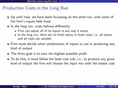
Short-Run versus Long-Run Costs
Production Costs in the Long Run
Up until now, we have been focussing on the short-run, with some ofthe firm’s inputs held fixed.
In the long run, costs behave differently
Firm can adjust all of its inputs in any way it wantsIn the long run, there are no fixed inputs or fixed costs; i.e. all inputsand all costs are variable
Firm must decide what combination of inputs to use in producing anylevel of output
The firms goal is to earn the highest possible profit
To do this, it must follow the least cost rule; i.e., to produce any givenlevel of output the firm will choose the input mix with the lowest cost
This yields a Long-Run Average Total Cost Curve
; i.e., therelationship between the output and the ATC when fixed costs arechosen to minimize total cost for each level of output.
Herriges (ISU) Ch. 12 Behind the Supply Curve Fall 2010 23 / 30

Short-Run versus Long-Run Costs
Production Costs in the Long Run
Up until now, we have been focussing on the short-run, with some ofthe firm’s inputs held fixed.
In the long run, costs behave differently
Firm can adjust all of its inputs in any way it wantsIn the long run, there are no fixed inputs or fixed costs; i.e. all inputsand all costs are variable
Firm must decide what combination of inputs to use in producing anylevel of output
The firms goal is to earn the highest possible profit
To do this, it must follow the least cost rule; i.e., to produce any givenlevel of output the firm will choose the input mix with the lowest cost
This yields a Long-Run Average Total Cost Curve; i.e., therelationship between the output and the ATC when fixed costs arechosen to minimize total cost for each level of output.
Herriges (ISU) Ch. 12 Behind the Supply Curve Fall 2010 23 / 30

Short-Run versus Long-Run Costs
Consider John’s Woodworking Shop
Suppose that in our first production function, we assumed that Johnhad only one set of tools (e.g., 1 table saw, 1 drill press, and 1 routertable).
We’ll call this one unit of capital
The tools (and the space to house his tools) constitute fixed costs forJohn in the short-run.
In the long-run, John must decide whether or not he wants to expandhis capital stock
The trade-off is that additional capital will avoid worker congestion,but imposes a large fixed cost on the firm.
At low levels of production, having just one set of tools is not a bindingconstraint and John would rather avoid the additional capital costs.At higher levels of production, additional capital will avoid congestionproblems and the capital costs are spread out over more units ofproduction.
Herriges (ISU) Ch. 12 Behind the Supply Curve Fall 2010 24 / 30
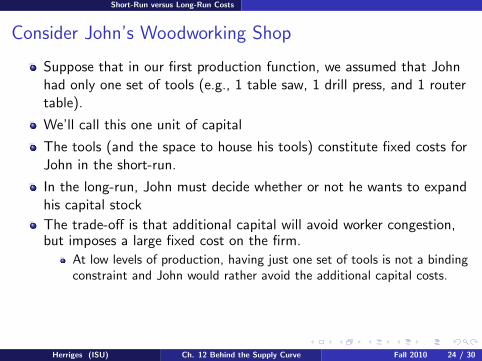
Short-Run versus Long-Run Costs
Consider John’s Woodworking Shop
Suppose that in our first production function, we assumed that Johnhad only one set of tools (e.g., 1 table saw, 1 drill press, and 1 routertable).
We’ll call this one unit of capital
The tools (and the space to house his tools) constitute fixed costs forJohn in the short-run.
In the long-run, John must decide whether or not he wants to expandhis capital stock
The trade-off is that additional capital will avoid worker congestion,but imposes a large fixed cost on the firm.
At low levels of production, having just one set of tools is not a bindingconstraint and John would rather avoid the additional capital costs.
At higher levels of production, additional capital will avoid congestionproblems and the capital costs are spread out over more units ofproduction.
Herriges (ISU) Ch. 12 Behind the Supply Curve Fall 2010 24 / 30

Short-Run versus Long-Run Costs
Consider John’s Woodworking Shop
Suppose that in our first production function, we assumed that Johnhad only one set of tools (e.g., 1 table saw, 1 drill press, and 1 routertable).
We’ll call this one unit of capital
The tools (and the space to house his tools) constitute fixed costs forJohn in the short-run.
In the long-run, John must decide whether or not he wants to expandhis capital stock
The trade-off is that additional capital will avoid worker congestion,but imposes a large fixed cost on the firm.
At low levels of production, having just one set of tools is not a bindingconstraint and John would rather avoid the additional capital costs.At higher levels of production, additional capital will avoid congestionproblems and the capital costs are spread out over more units ofproduction.
Herriges (ISU) Ch. 12 Behind the Supply Curve Fall 2010 24 / 30

Short-Run versus Long-Run Costs
Different Levels of Capital
Labor Units of CapitalUnits of Labor Capital = 1 Capital = 2 Capital = 3
0 0 0 0
1 10 10 102 35 39 393 80 92 1014 160 184 2025 193 284 3146 218 397 4397 239 443 5718 257 478 709
Herriges (ISU) Ch. 12 Behind the Supply Curve Fall 2010 25 / 30

Short-Run versus Long-Run Costs
Different Levels of Capital
Labor Units of CapitalUnits of Labor Capital = 1 Capital = 2 Capital = 3
0 0 0 01 10 10 10
2 35 39 393 80 92 1014 160 184 2025 193 284 3146 218 397 4397 239 443 5718 257 478 709
Herriges (ISU) Ch. 12 Behind the Supply Curve Fall 2010 25 / 30

Short-Run versus Long-Run Costs
Different Levels of Capital
Labor Units of CapitalUnits of Labor Capital = 1 Capital = 2 Capital = 3
0 0 0 01 10 10 102 35 39 39
3 80 92 1014 160 184 2025 193 284 3146 218 397 4397 239 443 5718 257 478 709
Herriges (ISU) Ch. 12 Behind the Supply Curve Fall 2010 25 / 30

Short-Run versus Long-Run Costs
Different Levels of Capital
Labor Units of CapitalUnits of Labor Capital = 1 Capital = 2 Capital = 3
0 0 0 01 10 10 102 35 39 393 80 92 101
4 160 184 2025 193 284 3146 218 397 4397 239 443 5718 257 478 709
Herriges (ISU) Ch. 12 Behind the Supply Curve Fall 2010 25 / 30
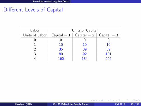
Short-Run versus Long-Run Costs
Different Levels of Capital
Labor Units of CapitalUnits of Labor Capital = 1 Capital = 2 Capital = 3
0 0 0 01 10 10 102 35 39 393 80 92 1014 160 184 202
5 193 284 3146 218 397 4397 239 443 5718 257 478 709
Herriges (ISU) Ch. 12 Behind the Supply Curve Fall 2010 25 / 30
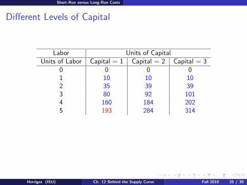
Short-Run versus Long-Run Costs
Different Levels of Capital
Labor Units of CapitalUnits of Labor Capital = 1 Capital = 2 Capital = 3
0 0 0 01 10 10 102 35 39 393 80 92 1014 160 184 2025 193 284 314
6 218 397 4397 239 443 5718 257 478 709
Herriges (ISU) Ch. 12 Behind the Supply Curve Fall 2010 25 / 30

Short-Run versus Long-Run Costs
Different Levels of Capital
Labor Units of CapitalUnits of Labor Capital = 1 Capital = 2 Capital = 3
0 0 0 01 10 10 102 35 39 393 80 92 1014 160 184 2025 193 284 3146 218 397 439
7 239 443 5718 257 478 709
Herriges (ISU) Ch. 12 Behind the Supply Curve Fall 2010 25 / 30
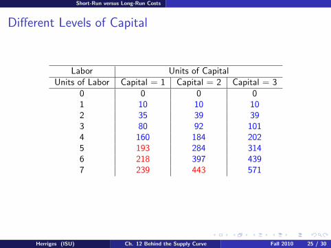
Short-Run versus Long-Run Costs
Different Levels of Capital
Labor Units of CapitalUnits of Labor Capital = 1 Capital = 2 Capital = 3
0 0 0 01 10 10 102 35 39 393 80 92 1014 160 184 2025 193 284 3146 218 397 4397 239 443 571
8 257 478 709
Herriges (ISU) Ch. 12 Behind the Supply Curve Fall 2010 25 / 30

Short-Run versus Long-Run Costs
Different Levels of Capital
Labor Units of CapitalUnits of Labor Capital = 1 Capital = 2 Capital = 3
0 0 0 01 10 10 102 35 39 393 80 92 1014 160 184 2025 193 284 3146 218 397 4397 239 443 5718 257 478 709
Herriges (ISU) Ch. 12 Behind the Supply Curve Fall 2010 25 / 30

Short-Run versus Long-Run Costs
The Corresponding ATC Figures are Given by
Herriges (ISU) Ch. 12 Behind the Supply Curve Fall 2010 26 / 30

Short-Run versus Long-Run Costs
The Corresponding ATC Figures are Given by
Herriges (ISU) Ch. 12 Behind the Supply Curve Fall 2010 26 / 30

Short-Run versus Long-Run Costs
The Corresponding ATC Figures are Given by
Herriges (ISU) Ch. 12 Behind the Supply Curve Fall 2010 26 / 30

Short-Run versus Long-Run Costs
John’s Capital Stock ChoiceThe level of capital stock John chooses depends on his expected level ofoutput
Herriges (ISU) Ch. 12 Behind the Supply Curve Fall 2010 27 / 30

Short-Run versus Long-Run Costs
John’s Capital Stock ChoiceThe level of capital stock John chooses depends on his expected level ofoutput
Herriges (ISU) Ch. 12 Behind the Supply Curve Fall 2010 27 / 30

Short-Run versus Long-Run Costs
John’s Capital Stock ChoiceThe level of capital stock John chooses depends on his expected level ofoutput
Herriges (ISU) Ch. 12 Behind the Supply Curve Fall 2010 27 / 30

Short-Run versus Long-Run Costs
John’s Capital Stock ChoiceThe level of capital stock John chooses depends on his expected level ofoutput
Herriges (ISU) Ch. 12 Behind the Supply Curve Fall 2010 27 / 30

Short-Run versus Long-Run Costs
John’s Capital Stock ChoiceThe level of capital stock John chooses depends on his expected level ofoutput
Herriges (ISU) Ch. 12 Behind the Supply Curve Fall 2010 27 / 30
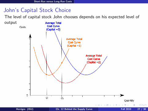
Short-Run versus Long-Run Costs
John’s Capital Stock ChoiceThe level of capital stock John chooses depends on his expected level ofoutput
Herriges (ISU) Ch. 12 Behind the Supply Curve Fall 2010 27 / 30

Short-Run versus Long-Run Costs
John’s Capital Stock ChoiceThe level of capital stock John chooses depends on his expected level ofoutput
Herriges (ISU) Ch. 12 Behind the Supply Curve Fall 2010 27 / 30

Short-Run versus Long-Run Costs
John’s Capital Stock ChoiceThe level of capital stock John chooses depends on his expected level ofoutput
Herriges (ISU) Ch. 12 Behind the Supply Curve Fall 2010 27 / 30

Short-Run versus Long-Run Costs
John’s Capital Stock ChoiceThe level of capital stock John chooses depends on his expected level ofoutput
Herriges (ISU) Ch. 12 Behind the Supply Curve Fall 2010 27 / 30

Short-Run versus Long-Run Costs
John’s Capital Stock ChoiceThe level of capital stock John chooses depends on his expected level ofoutput
Herriges (ISU) Ch. 12 Behind the Supply Curve Fall 2010 27 / 30

Short-Run versus Long-Run Costs
John’s Capital Stock ChoiceThe level of capital stock John chooses depends on his expected level ofoutput
Herriges (ISU) Ch. 12 Behind the Supply Curve Fall 2010 27 / 30

Short-Run versus Long-Run Costs
John’s Capital Stock ChoiceThe level of capital stock John chooses depends on his expected level ofoutput
Herriges (ISU) Ch. 12 Behind the Supply Curve Fall 2010 27 / 30

Short-Run versus Long-Run Costs
John’s Capital Stock ChoiceThe level of capital stock John chooses depends on his expected level ofoutput
Herriges (ISU) Ch. 12 Behind the Supply Curve Fall 2010 27 / 30

Short-Run versus Long-Run Costs
John’s Capital Stock ChoiceThe level of capital stock John chooses depends on his expected level ofoutput
Herriges (ISU) Ch. 12 Behind the Supply Curve Fall 2010 27 / 30

Short-Run versus Long-Run Costs
If Capital Stock Can be Varied Continuously, We Get
Herriges (ISU) Ch. 12 Behind the Supply Curve Fall 2010 28 / 30

Short-Run versus Long-Run Costs
Returns to Scale
LRATC curves for industries usually exhibit three basic phases:
1 Increasing Returns to Scale: Output range with declining LRATC
This is also known as economies of scaleEconomies of scale often arise due to the gains from specialization.The greatest opportunities for increased specialization occur when afirm is producing at a relatively low level of outputEconomies of scale can also arise due to minimum size requirements forcertain types of equipment.
2 Constant Returns to Scale: Output range with constant LRATC
Over some range of production, size may not matter and firms of thesame size will be equally cost-effective.
3 Decreasing Returns to Scale: Output range with increasing LRATC
This is also known as diseconomies of scaleAs output continues to increase, most firms will reach a point wherebigness begins to cause problemsThis is true even in the long run, when the firm is free to increase itsplant size as well as its workforceDiseconomies of scale are more likely at higher output levels
Herriges (ISU) Ch. 12 Behind the Supply Curve Fall 2010 29 / 30
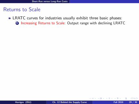
Short-Run versus Long-Run Costs
Returns to Scale
LRATC curves for industries usually exhibit three basic phases:1 Increasing Returns to Scale: Output range with declining LRATC
This is also known as economies of scale
Economies of scale often arise due to the gains from specialization.The greatest opportunities for increased specialization occur when afirm is producing at a relatively low level of outputEconomies of scale can also arise due to minimum size requirements forcertain types of equipment.
2 Constant Returns to Scale: Output range with constant LRATC
Over some range of production, size may not matter and firms of thesame size will be equally cost-effective.
3 Decreasing Returns to Scale: Output range with increasing LRATC
This is also known as diseconomies of scaleAs output continues to increase, most firms will reach a point wherebigness begins to cause problemsThis is true even in the long run, when the firm is free to increase itsplant size as well as its workforceDiseconomies of scale are more likely at higher output levels
Herriges (ISU) Ch. 12 Behind the Supply Curve Fall 2010 29 / 30

Short-Run versus Long-Run Costs
Returns to Scale
LRATC curves for industries usually exhibit three basic phases:1 Increasing Returns to Scale: Output range with declining LRATC
This is also known as economies of scaleEconomies of scale often arise due to the gains from specialization.
The greatest opportunities for increased specialization occur when afirm is producing at a relatively low level of outputEconomies of scale can also arise due to minimum size requirements forcertain types of equipment.
2 Constant Returns to Scale: Output range with constant LRATC
Over some range of production, size may not matter and firms of thesame size will be equally cost-effective.
3 Decreasing Returns to Scale: Output range with increasing LRATC
This is also known as diseconomies of scaleAs output continues to increase, most firms will reach a point wherebigness begins to cause problemsThis is true even in the long run, when the firm is free to increase itsplant size as well as its workforceDiseconomies of scale are more likely at higher output levels
Herriges (ISU) Ch. 12 Behind the Supply Curve Fall 2010 29 / 30

Short-Run versus Long-Run Costs
Returns to Scale
LRATC curves for industries usually exhibit three basic phases:1 Increasing Returns to Scale: Output range with declining LRATC
This is also known as economies of scaleEconomies of scale often arise due to the gains from specialization.The greatest opportunities for increased specialization occur when afirm is producing at a relatively low level of output
Economies of scale can also arise due to minimum size requirements forcertain types of equipment.
2 Constant Returns to Scale: Output range with constant LRATC
Over some range of production, size may not matter and firms of thesame size will be equally cost-effective.
3 Decreasing Returns to Scale: Output range with increasing LRATC
This is also known as diseconomies of scaleAs output continues to increase, most firms will reach a point wherebigness begins to cause problemsThis is true even in the long run, when the firm is free to increase itsplant size as well as its workforceDiseconomies of scale are more likely at higher output levels
Herriges (ISU) Ch. 12 Behind the Supply Curve Fall 2010 29 / 30

Short-Run versus Long-Run Costs
Returns to Scale
LRATC curves for industries usually exhibit three basic phases:1 Increasing Returns to Scale: Output range with declining LRATC
This is also known as economies of scaleEconomies of scale often arise due to the gains from specialization.The greatest opportunities for increased specialization occur when afirm is producing at a relatively low level of outputEconomies of scale can also arise due to minimum size requirements forcertain types of equipment.
2 Constant Returns to Scale: Output range with constant LRATC
Over some range of production, size may not matter and firms of thesame size will be equally cost-effective.
3 Decreasing Returns to Scale: Output range with increasing LRATC
This is also known as diseconomies of scaleAs output continues to increase, most firms will reach a point wherebigness begins to cause problemsThis is true even in the long run, when the firm is free to increase itsplant size as well as its workforceDiseconomies of scale are more likely at higher output levels
Herriges (ISU) Ch. 12 Behind the Supply Curve Fall 2010 29 / 30

Short-Run versus Long-Run Costs
Returns to Scale
LRATC curves for industries usually exhibit three basic phases:1 Increasing Returns to Scale: Output range with declining LRATC
This is also known as economies of scaleEconomies of scale often arise due to the gains from specialization.The greatest opportunities for increased specialization occur when afirm is producing at a relatively low level of outputEconomies of scale can also arise due to minimum size requirements forcertain types of equipment.
2 Constant Returns to Scale: Output range with constant LRATC
Over some range of production, size may not matter and firms of thesame size will be equally cost-effective.
3 Decreasing Returns to Scale: Output range with increasing LRATC
This is also known as diseconomies of scale
As output continues to increase, most firms will reach a point wherebigness begins to cause problemsThis is true even in the long run, when the firm is free to increase itsplant size as well as its workforceDiseconomies of scale are more likely at higher output levels
Herriges (ISU) Ch. 12 Behind the Supply Curve Fall 2010 29 / 30

Short-Run versus Long-Run Costs
Returns to Scale
LRATC curves for industries usually exhibit three basic phases:1 Increasing Returns to Scale: Output range with declining LRATC
This is also known as economies of scaleEconomies of scale often arise due to the gains from specialization.The greatest opportunities for increased specialization occur when afirm is producing at a relatively low level of outputEconomies of scale can also arise due to minimum size requirements forcertain types of equipment.
2 Constant Returns to Scale: Output range with constant LRATC
Over some range of production, size may not matter and firms of thesame size will be equally cost-effective.
3 Decreasing Returns to Scale: Output range with increasing LRATC
This is also known as diseconomies of scaleAs output continues to increase, most firms will reach a point wherebigness begins to cause problems
This is true even in the long run, when the firm is free to increase itsplant size as well as its workforceDiseconomies of scale are more likely at higher output levels
Herriges (ISU) Ch. 12 Behind the Supply Curve Fall 2010 29 / 30

Short-Run versus Long-Run Costs
Returns to Scale
LRATC curves for industries usually exhibit three basic phases:1 Increasing Returns to Scale: Output range with declining LRATC
This is also known as economies of scaleEconomies of scale often arise due to the gains from specialization.The greatest opportunities for increased specialization occur when afirm is producing at a relatively low level of outputEconomies of scale can also arise due to minimum size requirements forcertain types of equipment.
2 Constant Returns to Scale: Output range with constant LRATC
Over some range of production, size may not matter and firms of thesame size will be equally cost-effective.
3 Decreasing Returns to Scale: Output range with increasing LRATC
This is also known as diseconomies of scaleAs output continues to increase, most firms will reach a point wherebigness begins to cause problemsThis is true even in the long run, when the firm is free to increase itsplant size as well as its workforce
Diseconomies of scale are more likely at higher output levels
Herriges (ISU) Ch. 12 Behind the Supply Curve Fall 2010 29 / 30

Short-Run versus Long-Run Costs
Returns to Scale
LRATC curves for industries usually exhibit three basic phases:1 Increasing Returns to Scale: Output range with declining LRATC
This is also known as economies of scaleEconomies of scale often arise due to the gains from specialization.The greatest opportunities for increased specialization occur when afirm is producing at a relatively low level of outputEconomies of scale can also arise due to minimum size requirements forcertain types of equipment.
2 Constant Returns to Scale: Output range with constant LRATC
Over some range of production, size may not matter and firms of thesame size will be equally cost-effective.
3 Decreasing Returns to Scale: Output range with increasing LRATC
This is also known as diseconomies of scaleAs output continues to increase, most firms will reach a point wherebigness begins to cause problemsThis is true even in the long run, when the firm is free to increase itsplant size as well as its workforceDiseconomies of scale are more likely at higher output levels
Herriges (ISU) Ch. 12 Behind the Supply Curve Fall 2010 29 / 30
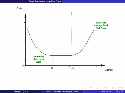
Short-Run versus Long-Run Costs
Herriges (ISU) Ch. 12 Behind the Supply Curve Fall 2010 30 / 30

Short-Run versus Long-Run Costs
Herriges (ISU) Ch. 12 Behind the Supply Curve Fall 2010 30 / 30
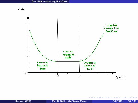
Short-Run versus Long-Run Costs
Herriges (ISU) Ch. 12 Behind the Supply Curve Fall 2010 30 / 30