ECDL Module 4 - UCL HEP Group · ECDL: Module 4 Spreadsheets ... (ECDL) Excel 2002 Part 1 is the...

ECDL Module 4 Document 353 Version 2

Information Systems EISD

Information Systems

Part of the Education & Information Support Division

Title: Excel 2002 (XP) Part 1

Authors: Rachel Healy and Fiona Strawbridge

Reference: Doc 353 v2

ECDL: Module 4 Spreadsheets (Part 1 of 2)

Date: September 2002

Revisions: Updated from Excel 97 to Excel 2002 (XP) - Aug 2002 by Fiona Strawbridge and Tamsin Griffith

Abstract

Microsoft Excel is a spreadsheet application used for manipulating and calculating numerical data, and forms part of the Microsoft Office XP suite application. This workbook is aimed at users who are new to spreadsheets and to the Excel package. It has been designed to accompany the Information Systems Excel 2002 (XP) Part 1 course (see www.ucl.ac.uk/is/training for course details) and it can be used as a self-paced tutorial. The European Computer Driving Licence (ECDL) Excel 2002 Part 1 is the first of two workbooks designed to cover the ECDL Module 4 Spreadsheet syllabus. It is one in a series of workbooks designed to cover the seven modules of the ECDL Syllabus (Version 3.0). For further information visit the ECDL web pages at www.ucl.ac.uk/is/training/ecdl.htm Pre-requisites It is assumed in this Workbook that you have the requisite keyboard skills and knowledge of a PC including file handling and data storage. It is also assumed that you are familiar with Windows and know how to use a mouse. If you are unfamiliar with any of these topics please consult the other workbooks in the series. Please Note Excel 2002 (XP) can be accessed from UCL Information Systems (IS) PC Workstations running WTS1. It is assumed in this Workbook that you are a registered user (i.e. you have an IS user ID and password) using a PC on the Information Systems WTS Service. Microsoft is a registered trademark and Windows is a trademark of Microsoft Corporation. Screen shots re-printed by permission from Microsoft Corporation.

1 WTS is the Managed PC Service. It provides a Windows 2000 environment.

Part 1 Excel

UCL Information Systems i

Contents

1. What is a Spreadsheet? ...................................................................................................1

1.1 The Excel Environment ..............................................................................................1 1.2 Task Panes ..................................................................................................................2 1.3 Workbooks and Worksheets .......................................................................................3 1.4 Accessing Commands.................................................................................................3 1.5 Moving around the Worksheet....................................................................................5

2. Help Features ...................................................................................................................7

2.1 Getting Help................................................................................................................7

3. Using a Worksheet ...........................................................................................................9

3.1 To Create a New Workbook .......................................................................................9 3.2 To Open a Workbook..................................................................................................9 3.3 Entering Data ............................................................................................................10 3.4 Data Entry Techniques..............................................................................................10 3.5 Entering Dates and Times.........................................................................................11 3.6 Entering a Series of Numbers or Dates.....................................................................12

4. Saving Your Work .........................................................................................................15

4.2 To Close a Workbook ...............................................................................................16 4.3 To Exit Excel ............................................................................................................16

5. Editing a Worksheet ......................................................................................................17

5.1 To Edit in the Formula Bar .......................................................................................17 5.2 To Edit in the Cell.....................................................................................................17 5.3 Selecting Data ...........................................................................................................18 5.4 Copying and Moving Data........................................................................................19 5.5 Deleting Data ............................................................................................................20 5.6 Deleting and Inserting Rows and Columns ..............................................................20 5.7 Undo and Redo .........................................................................................................21 5.8 Find and Replace.......................................................................................................21

6. Creating Simple Formulae ............................................................................................23

6.1 Essential Facts about Formulae ................................................................................23 6.2 Simple Formulae.......................................................................................................23 6.3 Copying Formulae ....................................................................................................25

7. Functions.........................................................................................................................27

7.1 Functions and Arguments .........................................................................................27 7.2 Using the Function Wizard .......................................................................................27 7.3 The Sum Function.....................................................................................................30 7.4 Statistical Functions ..................................................................................................31 7.5 Mathematical Functions............................................................................................31 7.6 Combining or Nesting Functions ..............................................................................32

8. Understanding Error Messages ....................................................................................33

9. Viewing Formulae..........................................................................................................34

Excel Part 1

ii UCL Information Systems

10. Formatting a Worksheet ...............................................................................................36

10.1 Changing Column Width ..........................................................................................36 10.2 Assigning a Number Format.....................................................................................37 10.3 More on Number Formats.........................................................................................39 10.4 To Set the Precision of Number Formats..................................................................39 10.5 Number Formats - Keyboard Shortcuts ....................................................................39 10.6 Formatting Characters...............................................................................................41 10.7 Borders, Patterns and Colours...................................................................................41 10.8 Aligning Data............................................................................................................42

11. Controlling the Worksheet Display..............................................................................45

11.1 To Freeze Horizontal or Vertical Titles Only...........................................................45 11.2 To Freeze both Horizontal and Vertical Titles .........................................................45 11.3 To Unfreeze Titles and Panes ...................................................................................45 11.4 To Hide a Column or Row........................................................................................45 11.5 To Reveal the Column or Row .................................................................................45 11.6 Splitting Panes ..........................................................................................................46 11.7 To Remove the Split .................................................................................................46

12. Preparing to Print ..........................................................................................................47

12.1 Page Setup: The Page Tab ........................................................................................47 12.2 Page Setup: The Margins Tab...................................................................................48 12.3 Page Setup: The Headers and Footers Tab ...............................................................49 12.4 Page Setup: The Sheet Tab .......................................................................................50 12.5 Print Preview.............................................................................................................51 12.6 Printing a Worksheet.................................................................................................52

13. Exercises..........................................................................................................................54

Part 1 Excel

UCL Information Systems iii

Toolbar Tip

Open

Conventions Used in this Workbook

The following table outlines the formatting conventions used in this workbook.

Commands Represented as Commands Courier regular Menu commands Buttons to press

Arial Narrow bold

Keys to press enclosed in square brackets e.g. [Ctrl] or [Shift]

Enter/Return key [Return] Key combinations

square brackets with combined keys linked with plus sign e.g. [Ctrl +C] hold down the Control key and press C

Key sequences press each key enclosed in brackets e.g. [→] [→] press right arrow key twice in succession

Toolbar Tips Where possible a toolbar shortcut has been provided, shown in a bubble alongside the relevant text. This button can be used instead of the menu method described in the text.

How to Use this Workbook This guide can be used as a reference or tutorial document. To facilitate the learning process, a series of practical tasks are contained within the text. It is recommended that you try each of these tasks as you progress through the workbook. For further practice and as a means of self-assessment, a number of additional staged exercises with solutions have been included. These should be attempted where recommended.

Training Files If you wish to attempt the exercises contained in this document and you are not using a training account it is necessary to download the training files used in this workbook from the IS training web site at: http://www.ucl.ac.uk/is/training/exercises.htm Full instructions on how to do this are provided on this web page.

Part 1 Excel

UCL Information Systems 1

1. What is a Spreadsheet?

A spreadsheet (called a workbook within Excel) is a powerful application which can be used to store, manipulate, calculate and analyse data such as numbers, text and formulae. An analogy can be drawn between a spreadsheet and an accountant’s ledger. A ledger is made up of many pages, each page arranged into a series of rows and columns. At its simplest level, a spreadsheet is used to enter numbers and perform simple calculations but the capabilities of Excel extend far beyond this. Excel provides a number of features including:

• A range of functions including mathematical, financial and other calculations. • A selection of tools to facilitate What If type analyses. • A Chart Wizard - to produce graphical representations of data held within

workbooks. • Graphics to highlight information in worksheets and charts. • Database features which enable sorting, filtering and analysing of information. • Macros to allow the user to automate routines.

There are many different practical applications for which a spreadsheet can be used. The obvious ones, which come to mind, are financial applications, such as maintaining budgets and accounts. Other applications include processing course marks, analysing results from experiments and maintaining lists and audits.

1.1 The Excel Environment

1. To launch Excel from the Start menu point to Programs and choose Excel. Your screen should look the same as the one below.

Figure 1-1 – The Excel Window

Status Bar

Menu Bar

A1

Row Heading

Scroll Bars

Name Box (Showing Active Cell)

Formatting Toolbar

Column Heading

Sheet Tab

Formula Bar

Standard Toolbar

Title bar

Task Pane

Sizing Buttons

Help Button

Excel Part 1

2 UCL Information Systems

Other Task Panes arrow

Figure 1-2 New Workbook Task Pane

2. The Formula bar, Status bar and the Scroll bars are all visible. Take a moment to

locate these on your screen. It is possible to change the look of the default environment, a number of the view options can be changed from the Tools menu under Options and View.

1.2 Task Panes

All of the Microsoft Office XP applications have a new feature called the Task Pane (visible in the right-hand part of the screen). This feature is a web-style command area which is an alternative to a dialogue box, and allows you to carry out certain basic operations or choose selected options. Most Office applications contain the following task panes: New File/Workbook/Document (the name varies with the application), Clipboard, Search and Insert ClipArt. § New Workbook– this task pane provides options for

starting a new workbook or opening an existing one. § Clipboard – this task pane is used for copying and

pasting multiple items into Excel, and between Excel and other Microsoft Office XP applications.

§ Search – this allows you to look for your work

(files, web pages etc.) in locations on your computer and on the web.

§ Insert Clipart – this task pane is used for inserting images and clipart into your

spreadsheet.

1.2.1 To Display the Task Pane

If the task pane is not visible down the right hand side of the application window, you can display it as follows: 1. From the View menu choose Task Pane. The task pane as shown in Figure 1-2 will display.

1.2.2 To change the Task Pane:

1. Click on the Other Task Panes arrow to display the options shown in Figure 1-3.

2. Select the required option. 3. Note that you can also use the arrows to go backwards and

forwards to previously displayed task panes. Figure 1-3 – Task Pane Options

Part 1 Excel


Press [Alt+E] to select the Edit menu. Press [Alt+E+D] to select Delete Press[Ctrl+F] to select Find

A1

1.3 Workbooks and Worksheets

On start up, Excel automatically loads a Workbook – Book1 as identified in the Title bar (see Figure 1-1). This workbook is a file in which you work and store your data. Each Workbook can contain a number of Worksheets. The default Workbook has three Worksheets, each having a tab to mark the sheet (i.e. Sheet1, Sheet2...). A worksheet is a grid like area divided into Columns and Rows. Columns are labelled A, B, C... and rows numbered 1, 2, 3...etc. Each worksheet is made up of 256 columns and 65,536 rows. The intersection of a column and a row is known as a cell. Each cell on a worksheet can be uniquely addressed by its column letter followed by its row number i.e. the first cell in the worksheet is A1. The active cell is now indicated by both the column and the row headings being highlighted in blue.

1.4 Accessing Commands

All commands may be accessed through the menu system although some are also available though buttons on toolbars and through the task pane.

1.4.1 Task Panes

Some commonly used commands are accessed through the task panes as described previously.

1.4.2 Menus

Commands may also be accessed through the Menu bar at the top of the Excel window.

Using the Mouse

1. Click on the menu item on the menu bar and click on the option you require in the drop down menu. Or

2. Right-click for context-sensitive options.

Using the Keyboard

There are two keyboard methods for accessing menu commands; using the [Alt] key, or using the [Ctrl] key. 1. Hold down the [Alt] key and press the letter

underlined in the menu item. For example, to access the Edit menu press [Alt + E]. OR

2. Use the [Ctrl] combinations where indicated in the menu. For example, use [Ctrl+c] to copy, [Ctrl+v] to paste etc. Note only some commands are available using the [Ctrl] key.

Figure 1-5 - Using Keyboard Shortcuts

Figure 1-4 - The Excel Worksheet

Excel Part 1


Shortcut Menus

A number of shortcut menus can be accessed in Excel by clicking on the right mouse button. These menus are context sensitive and also dynamic.

1.4.3 Toolbars

Toolbars provide a shortcut route to many commands. Using the mouse point and click on the required button. Different toolbars can be displayed and hidden at different times. By default the Standard and Formatting toolbars are displayed on the same line.

Figure 1-6 - Excel Toolbars

To Change the Toolbars displayed

1. Select the View menu and Toolbars.

2. Click in the check boxes to select the toolbars required from the list. The formula bar and status bar can also be selected in the View menu.

To Add Buttons to a Toolbar

1. Use the Toolbar Options arrow at the right of the toolbar to access additional toolbar options.

2. Choose the Add/Remove buttons option to customise your

toolbar. Note that once you have accessed a command from this list it will automatically be added to your toolbar.

Figure 1-7 – Toolbar Options

To Display Toolbars on Two Rows

1. Use the Toolbar Options arrow at the right of the toolbar to access additional toolbar options.

2. Choose the Show Buttons on Two Rows option display the Standard and Formatting

your toolbars on two rows.

Standard toolbar

Toolbar Options arrow

Formatting toolbar

Part 1 Excel


1.5 Moving around the Worksheet

1.5.1 Using the Mouse

Figure 1-8 - Moving Around the Excel Worksheet

1.5.2 Using the Keyboard

Shown below are some of the more commonly used keyboard shortcuts. A more exhaustive list can be found in Help.

The Arrow or Cursor Keys

á, ß, â, à

To Move One Cell at a time

Up, Left, Down, Right

[Ctrl + Home] moves to beginning of worksheet

[Ctrl + End] moves to last cell of current data region

[Ctrl + ß] moves left to end of current data region

[Ctrl + à] moves right to end of current data region

[Ctrl + á] moves to the next cell above containing data

[Ctrl + â] moves to the next cell below containing data

[Home] moves to column A of current row

[Page Up] moves one screen up

[Page Down] moves one screen down

[Alt + Page Up] moves one screen to the left

[Alt + Page Down] moves one screen to the right

The Pointer identifies the Active Cell

Use these scroll buttons to move from left to right in the sheet

Use the scroll box to move more quickly through the sheet

Use these scroll buttons to move up and down in the sheet

Use these buttons to navigate between different worksheets

Name box (Shows active cell)

Excel Part 1


1.5.3 Using the Name Box

The Name Box (see Figure 1-8) displays the address of the currently selected cell. You can use it to jump to any cell.

1. Click in the name box to highlight it. 2. Type in the required cell address and press [Return].

1.5.4 Using the Menu

1. From the Edit menu choose GoTo, and type the cell address into the GoTo dialogue box .

Task One – Orientation 1. Open Excel. 2. Identify the Status bar and the Formula bar. 3. Display the Standard and Formatting toolbars on one line. 4. Add a button of your choice to the Formatting toolbar. 5. Using a mouse method go to cell K99 and type the word Hello into the cell. 6. Now use a keyboard method to go to cell B10. 7. Identify the Task Pane and close it. Now re-display the Task Pane. 8. View the Help task pane. 9. Use the Name box method to return to cell K99 and delete its contents.

Part 1 Excel


2. Help Features

2.1 Getting Help

There are several ways to obtain help from within Excel: the Help Window, the Ask a Question list and What’s This (context sensitive help) are discussed here. Note that the Office Assistant is not installed on WTS. From the Help menu choose Microsoft Excel Help. The help window shown in Figure 2-1 will display. Select the type of help you require from the Contents, Answer Wizard or Index tabs. If the tabs do not appear, click the Use Contents to find instructions about broad categories. Contents are organised like a book’s table of contents. As you chose top-level contents, called chapters, you can see a list of more detailed subtopics from which to choose. The resulting help pages display in the right-hand part of the Help window. Use the Answer Wizard to enter questions in the box labelled “What would you like to do?”. Sub topics based on your response will be shown below. Again the corresponding help pages display to the right. Use the Index tab to locate specific topics – the Index is organised like a book’s index. Keywords for topics are organised alphabetically. You can either scroll through the list of keywords, or type the keyword you want to find, followed by [Enter]. You can then select from the topic choices shown. Again corresponding help pages display to the right.

Figure 2-1 – Microsoft Excel Help window

Auto Tile: arranges the Help window next to the main Excel window.

Hide: Hides the left hand part of the Help window.

Back & Forward: to move to previously visited Help options.

Print: to print the Help information.

Options: an alternative route to Hide, go Back, Forward, Print etc.

Excel Part 1


2.1.1 The Ask A Question List

This box is displayed in the upper right corner of the Excel window. You simply enter a question in plain English and press [Enter].

Figure 2-2 – The Ask A Question list

2.1.2 Help Using What’s This?

This provides context sensitive help. 1. From the Help menu click on What’s This?

2. Notice that the mouse pointer changes to show a large question mark . 3. Position the pointer in the document where help is required and click. A small Help

Window containing the relevant Help page will be displayed.

Task Two – Getting Help 1. Use the Answer Wizard to get help on how to Enter Data in Cells. 2. From the subtopic list which displays, view the entry on Entering Numbers, Dates and

Time. 3. In the Index tab, find help on toolbars. Display the index entry for moving toolbars. Is it

possible to move a toolbar? 4. From the Answer Wizard, get help on deleting cells. Enter the text delete cells and search.

Select Clear contents, formats or comments from the list of topics. What is the difference between using Edit, Clear from the menu, and clicking on the [Delete] key on the keyboard?

5. From the Contents tab select the Data in Worksheet topic and seek out more information

on entering data.

Part 1 Excel


Toolbar Tip

New

3. Using a Worksheet

3.1 To Create a New Workbook

1. From the File menu select New or select New Blank

Work book from the New Workbook task pane. A new worksheet is loaded.

3.2 To Open a Workbook

To open an existing workbook: 1. Click on More Workbooks from the New

Workbook task pane. The Open dialogue box appears (Figure 3-1).

2. In the Look In box select the appropriate Drive and Folder.

3. The available files are displayed in the window. Select the file required and click OK.

Figure 3-1 - Open Dialogue Box

Toolbar Tip

Open

Select the appropriate drive here - click on the arrow for drop down list and select

Files in current folder displayed here

Select File Type here – click on down arrow for drop down list

Excel Part 1


3.3 Entering Data

Data are always entered in the selected cell. Position the pointer in the cell required before entering data from the keyboard.

3.3.1 Types of Data

There are three types of data or information that may be entered into a worksheet:

Labels (text) Normally text used for headings or in lists.

Values (numbers) Raw data which are used in calculations i.e. numeric data only.

Formulae Arithmetic or mathematical expressions.

Values can be in one of many different formats and it is important for display and calculation purposes that the correct format is used. Normally labels are left aligned in cells, whilst values (numbers) are right aligned.

3.4 Data Entry Techniques

For faster data entry, highlight the range in the worksheet where data are to be entered and use the navigation keys shown here to navigate more efficiently.

[Tab] Enters data and moves right in the selected area. The cursor wraps to the left at the end of the selected range.

[Shift + Tab] Enters data and moves left in the selected area. The cursor wraps to the right at the end of the selected range.

[Enter] Enters data and moves down in the selected area. The cursor wraps back to the top of the selected range.

[Shift + Enter] Enters data and moves up in the selected area. The cursor wraps back to the end of the selected range.

[Ctrl + Enter] Enters the current data into the selected range.

Part 1 Excel


3.5 Entering Dates and Times

Excel recognises dates and times typed in most common formats. When you type a date or a time Excel converts the entry to a number. The number represents the number of days from the beginning of the century to the date typed. Time is recorded as a fraction of a 24 hour day. Correctly entered dates appear in the formula bar in the form dd/mm/yyyy e.g. 29/01/1999, regardless of how the cell is formatted. If Excel does not recognise your entry as a valid date or time format it is treated as text and, in an unformatted cell, will appear left aligned.

Acceptable Date Formats Acceptable Time Formats

31/12/97 14:53

31-Dec-97 14:53:35

31-Dec (the year from the system date is used)

2:53 PM

Dec-97 2:53:35 PM

31/12/97 14:53 31/12/97 14:53

In any of these date formats you can use a /, -, or space to separate elements.

If the 12 hour clock is used follow the time with an A, AM, P, or PM in either upper or lower case.

Date and Time Shortcuts

[Ctrl + ;] To quickly enter the current date in a cell

[Ctrl + :] To quickly enter the current time in a cell

[Ctrl + #] To format a date in the default date format

[Ctrl + @] To format a time in the default time format

Excel Part 1


Drag the Fill Handle down to extend the series

3.6 Entering a Series of Numbers or Dates

Excel makes it possible to generate automatically a series of numbers or dates using a facility called Autofill. It also offers the flexibility to enable the user to customise their own number and text series.

3.6.1 Working with Series

There are a number of time series that Excel will recognise:

Initial selection Extended series 9:00 10:00, 11:00, 12:00 Mon Tue, Wed, Thu Monday Tuesday, Wednesday, Thursday Jan Feb, Mar, Apr Jan, Apr Jul, Oct, Jan Jan-96, Apr-96 Jul-96, Oct-96, Jan-97 15-Jan, 15-Apr 15-Jul, 15-Oct 1994, 1995 1996, 1997, 1998

To enter a series of data using Autofill in Excel:

1. Enter the first item of data in the series.

2. Select the cell.

3. Drag the fill handle down or to the right to enclose

the area you want filled with the series, and release the mouse when finished. The enclosed area fills with the series selected.

3.6.2 AutoFill

The AutoFill feature extends several types of series as shown in the following table.

Initial selection Extended series Mon Tue, Wed, Thu,... 1-Jan, 1-Mar 1-May, 1-Jul, 1-Sep,... Qtr3 (or Q3 or Quarter3) Qtr4, Qtr1, Qtr2,... Product 1, Order Product 2, Order, Product 3, Order,... text1, textA text2, textA, text3, textA,... 1st Period 2nd Period, 3rd Period,... Product 1 Product 2, Product 3,... 1, 2 3, 4, 5, 6,... 1, 3, 4 5.66, 7.16, 8.66,...

Figure 3-2 Default Time Series

Part 1 Excel


3.6.3 To Create a Linear Series

1. Enter the first two items of data in the series in adjacent cells.

2. Select the two cells.

3. Drag the Fill Handle down or to the right to enclose the area you want filled with the series, and release the mouse when finished. The enclosed area fills with the series determined by the first two cells selected. Examples:

1, 2 3, 4, 5 2, 4 6, 8, 10 100, 90 80, 70

3.6.4 Creating a Custom Fill

1. Select the Tools menu and Options.

2. Select the Custom Lists tab.

3. Select New List in the Custom Lists box.

4. Select the List Entries box and type each item in the list. Press [Enter] to separate the items.

5. To add your List to the Custom Lists click on the Add button and OK.

Figure 3-3 - Custom Lists

3.6.5 To Add a List from a Worksheet

1. Select the range of cells in the worksheet containing the list. 2. Select the Tools menu and Options. The Options dialogue box appears.

Figure 3-4 - Creating a Custom List

Select the cells containing the list

Check the cell range in the Import List from Cells box and click on Import

The customised list will appear in the List Entries box ready for use

Excel Part 1


3. Select the Custom Lists tab. The range appears in the Import List from Cells box. 4. Choose the Import button. The selected list appears in the List Entries box. To accept the

list click on OK.

Task Three – Data Entry Techniques 1. Open Excel. 2. Enter the following data into the blank worksheet making use of the Fill Handle.

Series 1 Series 2 Series 3 Mon Tues Wed Thurs Fri

3. Experiment with creating other series using the Fill Handle. 4. Enter the current time using a shortcut method. 5. Enter today’s date using a shortcut method.

Part 1 Excel


4. Saving Your Work

It is good practice to save your work at regular intervals. 1. From the File menu select Save. When saving a worksheet for the first time the Save As dialogue box appears. This box prompts you to give the worksheet a filename and to select where the file is to be saved.

Figure 4-1 - Save As Dialogue Box

2. The first time you use Save you should check where the file is to be stored. On Managed and Cluster room PCs you have access to a number of different drives. The most important to remember is the r:\ drive which is your area on the network drive (staff also have access to the networked n:\ drive). Files saved here will be secure and can be accessed from any Managed or cluster room PC. To save your work on a floppy disk select the a:\ drive.

Give your file a name:

In the File Name box type a suitable filename. You are advised to avoid spaces in your filenames and to accept the default extension .xls. This is particularly important if you are sharing files with other users. Try to use meaningful names so files can be more readily identified at a later date.

4.1.1 Re-Saving

Once a file has been given a name you can use the Save command and this will automatically update your old file.

4.1.2 Save As

Use the Save As command when you do not wish to overwrite an existing file, but wish to save your work in a new file with a different name. 1. From the File menu, click Save As. Select the required Drive and Folder.

2. Enter the new filename and click Save.

Toolbar Tip

Save

Select a drive here

Enter your filename here

Excel Part 1


4.2 To Close a Workbook

It is always good practice to close a workbook when you have finished working on it – but don’t forget to save it first. 1. From the File menu, click Close.

Closing a workbook before it is saved calls up a dialogue box prompting you to Save any changes.

Figure 4-2 - Save Changes

4.3 To Exit Excel

It is good practice to Save and Close your workbook before exiting. When you have done this 1. From the File menu select Exit. 2. Wait as Excel closes down.

Task Four – More Data Entry 1. Save the worksheet you created in the previous task in the

r:/training.dir/Excelp1 folder as series.xls and close the file. 2. Create a new worksheet and enter the data as shown in the figure below.

3. Save the file with the name summary.xls in the r:\training.dir\excelp1

folder.

4. Close the file without exiting Excel.

5. Open the file summary.xls again.

Part 1 Excel


5. Editing a Worksheet

Data can be edited using the Backspace [←] and [Delete] keys found on the keyboard.

5.1 To Edit in the Formula Bar

Figure 5-1 - Formula Bar

1. Position the pointer in the cell to be changed (the contents of the cell are displayed in

the formula bar). 2. Click in the formula bar and the cursor appears ready for editing. 3. On completion press [Return] or click on the Tick mark in the Formula bar.

5.2 To Edit in the Cell

1. Select the cell to be changed by clicking on it.

2. Double click in the cell Or Press [F2] to edit.

Notice that the cursor appears in the cell ready for editing.

3. On completion press [Return] or click on the Tick mark in the Formula bar to update

the changes.

Figure 5-2 - Editing Cells

Cell contents of active cell displayed in formula bar

Cursor appears in cell ready for editing

Cancel Button Enter Button

Function Button

Excel Part 1


5.3 Selecting Data

Before we can manipulate data in a worksheet it is necessary to identify the data first. This is done by selecting (highlighting) the required data, as explained below.

5.3.1 To Select a Cell

1. A single cell is selected by clicking the pointer in the required cell.

5.3.2 To Select a Block of Cells

1. Position the pointer in the top left-hand corner of the block.

2. Hold down the left mouse button and drag the pointer over the desired area.

3. Release the mouse button when the chosen area is selected. Notice that once an area has been selected the range is highlighted on the sheet in reverse video (i.e. white on black) except the first cell or active cell in the range.

5.3.3 To Select a Column or Row in a Worksheet

1. Click in the Column or Row heading. 2. The column or row will be highlighted.

Note that you can use the [Shift+Space] keyboard shortcut to select an entire row, or [Ctrl+ Space] to select an entire column.

Figure 5-3 - Selecting Data

5.3.4 To Select All Cells in a Worksheet

1. Click in the Select All box as shown in the figure above or use [CTRL+a].

Select All

Click here to select row 3

Click here to select column C

Part 1 Excel


5.4 Copying and Moving Data

5.4.1 To Copy Data

1. Select the cell(s) to be copied. 2. From the Edit menu select Copy or use [Ctrl+C] 3. Move the pointer to the new location. 4. From the Edit menu select Paste or use [Ctrl+V].

5.4.2 To Move Data

1. Select the cell(s) to be moved.

2. From the Edit menu select Cut or use [Ctrl+X]. The cells which have just been cut do not disappear but are outlined with a moving border.

3. Move the pointer to the new location.

4. From the Edit menu select Paste. Note: You can use the right mouse button to access the shortcut menus, where you will find the copy, paste and cut commands.

Task Five – Editing Data 1. Open the file summary.xls created in the previous task. 2. An error has been made in the title. Edit this to read Quarterly Summary. 3. A mistake has also been made in the data for the South in Qtr 3, edit this to read

45000.

4. The values for Qtr 4 are missing in the spreadsheet. Copy the values from Qtr 2 and Paste them in the column for Qtr 4.

5. Save the file with the same name summary.xls

Toolbar Tip

Copy Paste

Toolbar Tip

Cut Paste

Excel Part 1


5.5 Deleting Data

1. Select the cells to be deleted.

2. Press the [Delete] key – on the keyboard. Or From the Edit menu select Clear and choose Contents .

Note: It is the contents of the cells and not the actual cells which are deleted. To delete cells see the next section – Deleting and Inserting Rows and Columns.

5.6 Deleting and Inserting Rows and Columns

5.6.1 Deleting Rows and Columns

1. Position the pointer in a cell in the required row or column.

2. From the Edit menu choose Delete. The Delete dialogue box appears.

3. Choose Entire Row or Entire Column as required and click OK.

Figure 5-4 - Delete Dialogue

5.6.2 Inserting Rows and Columns

1. Position pointer in a cell in the required row or column.

2. Click on the Insert menu and choose Rows or Columns. Note: New rows are inserted above the pointer and new columns to the left of the pointer.

Select Entire row or Entire column

Part 1 Excel


5.7 Undo and Redo

When you make a mistake or change your mind you can use the Undo command to reverse your last commands or actions. Redo repeats your last command or action.

5.7.1 To Undo

1. Click on the Edit menu and choose Undo. The Undo command changes to show the most recent command or action. If the Undo command is unavailable the words ‘Can’t Undo’ appear greyed out in the menu.

2. To reverse more than one action at a time, click on the drop-down arrow beside the

undo button, and then click the actions you want to undo.

5.7.2 To Redo

1. From the Edit menu choose Redo. If the Redo command is unavailable the words ‘Can’t Repeat’ appear greyed out in the menu.

5.8 Find and Replace

The Find and Replace functions in Excel 2002 are more powerful than in Excel 97. Figure 5-5 shows the new interface. You can specify that you only match cells with the same case formatting as the text in the Find What box using the Match case tick box. You can also use the Format buttons to specify formats to search for, and formats to apply to the replacement.

Figure 5-5 – Find and Replace window

The Within box allows to search either a worksheet or workbook, and the Search box allows you to search either by row or column.

Toolbar Tip

Undo Repeat

Excel Part 1


The Find All button is a powerful new tool which produces a list of matches, including their worksheet and cell location, and whether the cell contains a value or a formula (Figure 5-6). You can go to any of the matched cells simply by clicking in the list.

Figure 5-6 – List of matches using Find All button

Task Six – More Editing Further data for the workbook summary.xls has been received from two new regions. 1. Open the file summary.xls created in the previous task.

2. Insert two new rows under the headings Qtr 1, Qtr 2 etc.

3. Enter the labels and data for the regions Scotland and Wales as shown.

4. Reposition the data for the East, so that it follows the South as shown above. 5. Search for Qtr and replace all instances with Quarter, using the Find All button. 6. Save the file with the same name, summary.xls and close the workbook.

Part 1 Excel


6. Creating Simple Formulae

Formulae allow the calculation of data or values in the Worksheet. These calculations range from simple arithmetic (addition, multiplication etc.) to more complex statistical, logical and database functions. In this workbook we will use some of the more simple arithmetic and statistical formulae and functions.

6.1 Essential Facts about Formulae

• Formulae always start with an = (equals) sign • Formulae are always placed in the cell where the result is to be displayed. • The result is displayed in the cell when the Tick button on the Formula bar is clicked,

or the [Return] key is pressed, or when the insertion point is moved to another cell.

Figure 6-1 - Entering Formulae

• Formulae should reference the Cell Address not the Cell Contents i.e. to add the two numbers shown in the figure above the correct formula is:

=A1+A2 not =10+15

• When the contents of a cell referenced in a formula change, the formula automatically calculates and displays the new result i.e. if the value in cell A1 is changed to 15 in the example above, the formula automatically recalculates to display the result 30.

6.2 Simple Formulae

Examples of formulae used for common arithmetic operations are shown in the table below:

Operator Description Excel Formula Example

+ Addition = A1+A2 add A1 and A2 3+2 = 5

- Subtraction = A1-A2 subtract A2 from A1 3 – 2 = 1

* Multiplication = A1*A2 multiply A1 by A2 3 * 2 = 6

/ Division = A1/A2 divide A1 by A2 3 / 2 = 1.5

^ Exponential = A1^A2 raise A1 to the power A2 3 ^ 2 = 9

Click here to show the result or press [Return]

Excel Part 1


% Percentage = A1 % express A1 as a percentage 3 % = 0.03

These operations can also be combined together. For example: = (A1-A2)/(A1+A2)

Or = (A1+B2–D4)*50 Use brackets to ensure that the different parts of the formula are calculated in the correct order. For example =(3+2)*4 is not the same as =3+2*4. Excel evaluates operators following the conventional rules (BODMAS):

( ) brackets first / and * division and multiplication + and – addition and subtraction

Take care to observe these rules when creating your own formulae. The incorrect syntax will result in error.

Formulae Result =(3+2)*4 20

=3+2*4 11

Task Seven – Simple Arithmetic In this task you will create basic formulae involving simple calculations on a pair of values. The sums involved are intentionally simple to allow you to check that your answers are correct using a little mental arithmetic. 1. Enter the following data into a new blank

workbook. Leave the cells containing the word formula empty for now:

2. Enter a formula to add together the contents of cells B3 and B4. Place the result in B6. 3. Enter a formula to subtract the contents of cells B4 from B3. Place the result in cell B7. 4. Enter a formula to multiply the contents of cell B3 by B4. Place the result in cell B8. 5. Enter a formula to divide the contents of cell B3 by B4. Place the result in B9.

Part 1 Excel


6. Do a quick check that your answers are correct, the save the file as maths.xls in the r:\training.dir\excelp1 folder.

6.3 Copying Formulae

Formulae can be copied using the Copy and Paste buttons in the same way as data can be copied in a worksheet. 1. Select the cell containing the formula to be copied.

2. From the Edit menu choose Copy (or use the Copy button).

3. Move the pointer to the new location.

4. From the Edit menu choose Paste (or use the Paste button).

Note how the cell references change as we copy the formula from cell A2 to cell A3 to cell A4 in the figure below. =A1 becomes =A2.

Figure 6-2 - Copying Formulae

Note how the cell references change as we copy the formula from cell A2 to cell B2 to cell C2 in the figure below. =A1 becomes =B1.

Figure 6-3 - Relative Referencing

When a formula is copied, it is applied relative to the new range. • Therefore the formula =A1 will become =A2 when it is copied to the next row • And the formula =A1 and will become =B1 when it is copied to the next column.

Notice how the reference changes by one row relative to its starting position

Notice how the reference changes by one column relative to its starting position

Excel Part 1


If this is unclear, accept that it is possible to copy formulae as Excel automatically changes the references for you. As you become more familiar with Excel this concept of referencing should become more familiar to you.

Task Eight – Copying Formulae 1. Open the maths.xls workbook created in the previous task. 2. Modify the worksheet by adding two new sets of values as shown below in cells C3,

C4, D3, and D4

3. Copy each of the formulae in Column B to Columns C and D. 4. Click in cell C6 and check that the formula is correct (when you click in the cell you

will see the formula rather than the result). It should be = C3 + C4 5. Check that the copied formulae have done what you needed using a bit of mental

arithmetic. 6. Save and close the workbook.

Part 1 Excel


7. Functions

You have seen how Excel allows you to enter formulae, to perform simple arithmetic operations on values in a worksheet. Excel also provides many built-in Functions which automate a number of different types of calculation. Functions are pre-programmed formulae – you are probably already familiar with the use of functions on a calculator (for example, the square-root function, trigonometric functions, logarithms etc.). Excel has more than 300 functions covering a range of statistical, mathematical, financial and logical operations. If you have many numbers in a group of cells that you wish to combine in a formula, typing the formula becomes laborious. Using a function offers a shortcut method. Examples of the most commonly used functions include the Average function, which calculates the average of a group of cell values, the Sum function, which adds together a group of cell values, and the Min and Max functions, which determine the lowest and highest values in a group of cells. If you know the name of a function, you can simply type it in together with the “argument” or range of cells you want to apply it to. However, an easy way to work with functions is through the Function Wizard.

7.1 Functions and Arguments

Functions are usually written with the equals sign (=) followed by the Function Name and then parentheses containing the Argument. Usually the argument just contains the range of cells which the function will operate on. For example, the Average function is written as:

= AVERAGE(A1:A4) The argument of a function is placed in brackets. To specify a range of cells a colon is used between the first and the last cell address. For example, (A1:A4) will specify cells A1, A2, A3 and A4.

7.2 Using the Function Wizard

1. Position the pointer in the cell which is to contain the result.

2. From the Insert menu select Function or click the

Function Wizard button on the Formula bar. The Insert Function dialogue box is displayed as shown.

Toolbar Tip

Function Wizard

Function Name

Argument

Excel Part 1


Figure 7-1 - Function Wizard

3. Note that using the Search for a function box you can type a description of what you

want to do. See Figure 7-1. The Most Recently Used category often offers the most likely choices. The functions in the selected category are shown in the lower half of the window.

Figure 7-2 - Categories in the Function Wizard.

Type in a brief description of what you want to do in the Search for a function box, or select a suitable Category and the Function Name required. 4. If in this example we choose AVERAGE and click on OK, the Function Arguments

dialogue box will display as shown in Figure 7-3. It may well obscure the part of the worksheet you want to work on. However it can be moved simply by clicking and dragging anywhere in the grey shaded box. It can also be shrunk by clicking on the “shrink/enlarge” button.

5. Note that the Function Wizard automatically guesses the range of cells to be used in the

calculation (A1:A2 in the example below). Click OK if this is correct. Alternatively type the range in, or highlight the cells required in the worksheet.

Part 1 Excel


Figure 7-3 - Average Function

6. Notice that a moving border appears around the specified cells as the range is entered in the dialogue box. Click on OK to complete.

7. You can view the completed formula by clicking in the cell, and looking at the contents

of the Formula Bar.

Task Nine - Functions 1. Open the summary.xls file last used in Task Five. Add a sixth column to the

worksheet and label this Average. You will use the Function Wizard to calculate the Average value for each region.

2. Position the pointer in cell F4 and click on the Function Wizard button. Select the

AVERAGE function and click on OK.

3. Highlight the range B4:E4 in the worksheet (if this range has not already been added automatically).

4. Click on OK to complete. Check that the formula is correct and copy it to the remaining rows in the column.

5. Save the file.

Shrink/Enlarge button

Excel Part 1


7.3 The Sum Function

A particularly useful function is the Sum function. This will simply add together a range of cell values. The formula: = A1+A2+A3+A4+A5+A6+A7+A8 can be replaced by: = SUM(A1:A8) This adds up the contents of the cells A1 to A8.

How to use the SUM function

• The function can be typed at the keyboard like any other formula.

• The formula can be created with the Function Wizard (see section 7.2).

• The SUM formula can be created using the AutoSum button (this is the easiest method).

7.3.1 To Use AutoSum

To ensure that AutoSum sums the required cells it is best to specify the cell range yourself, to do this: 1. Highlight a range including the cells to be

summed and one empty cell at the end of the range in which the result is to be placed. E.g. B4:B8

2. Click on the AutoSum button. The formulae is

placed in cell B8.

Figure 7-4 - Specifying the Cell Range for AutoSum

Alternatively select the cell to contain the result and then click on the AutoSum button. Excel automatically guesses at the range of cell references that you wish to sum (these can be amended if necessary). Always check automatically generated formulae before accepting them as Excel doesn’t always guess correctly which cells to sum.

Task Ten – The Sum Function 1. Open the file summary.xls and enter a formula using the AutoSum button to calculate

the Totals for each of the Quarters in the worksheet. Try doing this in two slightly different ways:

• Highlight the range B4:B10. Note this range includes an empty cell. Click on the AutoSum button. Look at the formula generated.

• Click in cell C10 and click on the AutoSum button. Check the formula is correct. Note that the second method is quicker, but also more prone to error - always check the formula.

2. Copy the formula in cell C10 to the remaining columns. Save the file.

Toolbar Tip

AutoSum

Part 1 Excel


7.4 Statistical Functions

Some common statistical functions which you may find useful are listed below.

Function Example Description

MAX MAX(C1:C10) Finds the largest cell value in the specified range of cells.

MIN MIN(C1:C10) Finds the smallest cell value in the specified range of cells.

AVERAGE AVERAGE(C1:10) Finds the average cell value in the specified range of cells.

MEDIAN MEDIAN(C1:C10) Finds the median or middle value in the specified range of cells.

STDEV STDEV(C1:C10) Finds the standard deviation of the values in a range of cells.

COUNT COUNT(C1:C10) Counts the number of cells containing numbers.

COUNTA COUNTA(C1:C10) Counts the number of cells containing numbers or letters (i.e. the number of non-blank cells).

COUNTBLANK COUNTBLANK(C1:C10) Counts the number of blank cells.

COUNTIF COUNTIF(C1:C10, “>99”)

or

COUNTIF(C1:C10, “pass”)

Counts the number of cells meeting a specified criterion (the first example will count the number of cells whose values are greater than 99; the second counts the number containing the word “pass”).

7.5 Mathematical Functions

Some common mathematical functions you may find useful are listed below.

Function name Example Description

ROUND ROUND(C1, 2) Rounds the cell value to the specified number of decimal places (2 in this example; use 0 to get a whole number).

SQRT SQRT(C1) Calculates the square root of a cell value.

RADIANS RADIANS(C1) Converts angle from degrees to radians.

SIN SIN(C1) Calculates the Sine of an angle (in radians – use the RADIANS function to convert degrees into radians). Other trigonometric functions include COS and TAN.

Excel Part 1


Task Eleven – Count Functions 1. Working with the Summary.xls file again, use one of the COUNT functions to count the

number of cells in the summary worksheet containing numerical data. Place the answer in cell A11.

2. Use one of the COUNT functions to count the number of cells in the summary worksheet containing either numerical or text data (i.e. non-blank cells). Place the answer in cell A12.

3. Use one of the COUNT functions to count the number of cells containing values smaller

than 50000. Place the answer in cell A13.

7.6 Combining or Nesting Functions

Sometimes you may want to use more than one function at once. For example, if you use AVERAGE to calculate the average of a group of prices, you might end up with a result with too many decimal places (two decimal places might be more appropriate than three). You might wish to round the result to a set number of decimal places, using the ROUND function. It is possible to combine the use of AVERAGE and ROUND in the same formula. The average calculation is shown here: To display the average price in pounds and pence (two decimal places) you might use the ROUND function as shown here: Or you could simplify things by combining the two as shown here:

Part 1 Excel


8. Understanding Error Messages

Excel may display error messages if your formulae or functions contain mistakes (note that it will not detect all errors in calculations. It is always worth checking the result of your formulae by hand if the formula is at all complex. Excel’s error messages are contain a # symbol followed by a diagnostic word (see table below). In some cases, the cell with an error in it has a small green arrow in the corner. In such cases if you click in the cell a yellow symbol with an explanation mark appears. Click the exclamation mark for options to help you trace the source of the error.

Figure 8-1 – Tracing Errors

Typical Errors and Their Causes

###### The column is not wide enough to display data (for numbers). Date or time may be negative.

#VALUE! Occurs when the wrong type of argument is used in a function or formula. For example, there is text in a formula that requires a number or logical value.

#DIV/0! Occurs when a number is divided by zero.

#NAME? Occurs when Excel doesn’t recognise text in a formula (e.g. misspelling a function name or cell reference).

#N/A Occurs when a value is not available to a formula or function – perhaps data are missing.

#REF! Occurs when a cell reference is not valid – perhaps the cell has been deleted.

#NUM! Occurs when a number is invalid – perhaps a price has been entered with the £ sign, or a formula results in a number too big or too small for Excel to display.

Circular reference

This happens when the formula points to the cell in which the result is to be displayed, e.g., placing the formula =SUM(A1:A2) into cell A2.

Green triangle

Yellow symbol with exclamation mark

Options for dealing with error

Cell containing error message

Excel Part 1


9. Viewing Formulae

Sometimes you may want to view the actual formulae in your worksheet, rather than the numerical results of the formulae. This can be particularly useful if you are getting error messages and need to examine the formulae. To view the formulae: 1. From the Tools menu choose Options… to reveal the Options window (Figure 9-1). 2. Select the View tab, and click the Formulas check box and OK.

Figure 9-1 – Options Window – View Tab

3. All formulae in the worksheet will display in full as shown below (this can be useful for

trouble-shooting if your calculations don’t seem to be working – you can print out the formulae for closer inspection). Notice how the columns automatically widen to accommodate the formula.

Figure 9-2 – Formulae Displayed in Worksheet

4. You can turn off the formula display using the same check box in the Options window.

Notice how the columns shrink again to their original width.

Formulas

Part 1 Excel


Task Twelve – Viewing Formulae 1. Open the summary.xls workbook. 2. Use the Options window to display the formulae in the worksheet. Notice how the

columns containing the formulae widen to accommodate them. 3. Now use the Options window again to turn off the formula display. Notice how the

columns containing the formulae shrink back to size again. 4. Save the file with the same name summary.xls.

You are now ready to try Exercises 1-3.

Excel Part 1


10. Formatting a Worksheet

All worksheets start with a number of predefined formats. As you work you may need to change some of these formats to suit your own needs. In this section we will look at some of the more common formatting options available.

10.1 Changing Column Width

1. Position the pointer in the column to be changed.

2. From the Format, menu point to Column and Width.

3. The Column Width dialogue box appears displaying the default width.

Figure 10-1 - Changing Column Width from the Menu

4. Type the new width required in the Column Width box and click OK.

10.1.1 Short Cut Method

1. Position the pointer in the column heading to the right of the column to be changed.

2. When the pointer changes shape to a double-headed arrow, click and hold down the left

mouse button and drag the pointer to the width required and release the mouse button.

Figure 10-2 - Changing Column Width using the Mouse

10.1.2 AutoFit

To set the column widths automatically: 1. Position the pointer on the right border of the column heading as above.

2. Double click the left mouse button. The width will be set automatically to fit the widest

cell entry in that column.

Current width is displayed

The # symbol shows where columns are too narrow to display all the data.

Text will be hidden where there is insufficient room to display labels (see full label displayed in formula bar).

Double-headed arrow appears as pointer is positioned in the border between two columns. Notice the dotted line which appears between the columns.

Part 1 Excel


10.2 Assigning a Number Format

Excel applies a General number format by default, this format displays values exactly as they are entered into the worksheet. In this section we will see how we can specify different number formats. 1. Select the cells you wish to format in the

worksheet.

2. From the Format menu select Cells. The Format Cells dialogue box appears.

3. From the Number tab select the category required e.g. Number category as shown here.

4. Specify the required format. (For the Number format you will need to enter the required number of Decimal places, click to select or deselect the Use 1000 Separator (,) and the display option for Negative numbers).

Figure 10-3 - Format Cells Window

10.2.1 Formatting Toolbar Options

Some of the most commonly used formats can be applied from the Formatting Toolbar.

Button Format Example

Currency Style £9,999.00

Percent 0.9 becomes 90%

Comma Style 9,999,999.00

Increase Decimal 9.00 becomes 9.000

Decrease Decimal 9.00 becomes 9.0

10.2.2 To Remove Cell Formats

1. Select the area where the format is to be removed.

2. From the Edit menu point to Clear and choose Formats.

Or alternatively reset the format style to General: 1. From the Format menu select Cells.

2. Select the General category and click OK.

Excel Part 1


Task Thirteen –Formatting 1. Open the file summary.xls.

2. Some of the region names in the worksheet have been changed. Edit the labels to show

these changes. The new labels are: Northern Region Southern Region Eastern Region Western Region

3. Change the column width to reveal the full labels. 4. Format the values in the worksheet to a Currency format. Select two Decimal places,

the £ Symbol and accept the default style given for Negative numbers. 5. Change the width of column C to roughly width:5.00.

What happens to the numbers displayed in the column? Why is this? 6. Change the width of column C back using AutoFit. 7. Save the file. You are now ready to do Exercises 4 and 5.

Part 1 Excel


10.3 More on Number Formats

Care must be taken when working with formatted numbers. It is important to remember that formatted numbers, i.e. the numbers which appear on the screen, may not be the same as the value stored in the cell or the numbers used in calculations. The discrepancy can cause the displayed results to be different from the manually calculated answers. Look at the example illustrated in Figure 10-4. There are two columns of numbers which appear to be the same, the first column adds up to 95 but the second column adds up to 100. Take a close look at the value stored in cell A1, as displayed in the formula bar. The value stored in all the cells in the first column is actually 9.5 this has been formatted to appear as a whole number (integer). The calculation is actually correct (10*9.5=95), although it does appear to be incorrect. The problem can be avoided by using number formats cautiously or it can be resolved by setting the precision for the entire worksheet.

Figure 10-4 - Number Formats

10.4 To Set the Precision of Number Formats

For an entire Worksheet: 1. Choose the Tools menu, Options command and select the Calculation tab.

2. Choose the Precision As Displayed box and OK.

When you choose OK you are warned that constant numbers throughout the worksheet will be rounded permanently to match cell formatting.

10.5 Number Formats - Keyboard Shortcuts

Number Format Shortcut Key General [Shift + Ctrl + ~] #,##0.00 [Shift + Ctrl + !] £#,##0.00;(£#,##0.00) [Shift + Ctrl + $] 0% [Shift + Ctrl + %] 0.00E+00 [Shift + Ctrl + ^]

Excel Part 1


Task Fourteen 1. Enter the following numbers into cells A1:A4 in a new worksheet:

5.5 5.5 5.5 5.5

2. Format the cells to display no decimal places. What happens to the numbers displayed? 3. Enter a formula in cell A5 to calculate the average of the values in cells A1:A4. 4. Examine the result of this calculation in cell A5. How many decimal places are

displayed? 5. Now set the format of cell A5 to display two decimal places. What happens to the

result? 6. Finally, set the precision of the entire worksheet to display Precision as Displayed

using the Options menu. 7. Save the file as number.xls and close it.

Part 1 Excel


10.6 Formatting Characters

Excel has the same range of basic Character formats as are available in the other Office applications.

1. Select the cells to be changed.

2. From the Format menu choose Cells. The Format Cells dialogue box appears as shown

below. 3. Choose the Font tab and select the required settings. The Font type, Style and Size as

well as Colour and other Effects can be selected, as shown below.

Figure 10-5 - Character Formats

10.7 Borders, Patterns and Colours

The appearance of the worksheet can be further enhanced with the use of borders and colour. 1. From the Format menu choose Cells and select the

appropriate tab, either Border, Patterns or Font.

Toolbar Tip

Border Fill Colour Font Colour

Toolbar Tip

Font Font size

Bold Italic Underline

Select Font type here

Select Font size here

Font tab selected

Select Font style here

Excel Part 1


10.8 Aligning Data

By default Excel automatically aligns text to the left and numbers to the right of the cell. We can change these defaults as shown below.

1.1.1 Horizontal and Vertical Alignment

There are a number of different vertical and horizontal alignment options to choose from:

Horizontal Alignment General, Left, Centre, Right, Fill, Justify and Centre Across Selection (Merge and Centre)

Vertical Alignment Top, Centre, Bottom and Justify. 1. Select the cells to be aligned.

2. From the Format menu choose Cells.

The Format Cells dialogue appears as shown below. 3. Choose the Alignment tab. 4. Select the required options from the Horizontal and Vertical boxes and click OK.

Figure 10-6 - Alignment Options

Toolbar Tip

Left Centre Right

Alignment tab

Select your choice of horizontal alignment here

Vertical alignment

Text wrapping

Part 1 Excel


10.8.1 Merge and Centre

This option allows you to centre a heading across a range of cells. 1. Select the range of cells. 2. From the Format Cells dialogue (as above) in the Text

Control box, choose Merge Cells. (The cells are merged together as if they are one).

3. To centre the text in the cells click on the Centre button. 4. To undo Merge and Centre formatting, select the area across which the data is centred,

and in Format Cells choose General from the Horizontal Alignment options. Note: Using Merge and Centre alters the way that ranges can be selected in the worksheet. In

particular it can prevent simple operations like copying and pasting columns. For this reason it is best to merge and centre only as a final step before printing.

10.8.2 More Alignment Options

Text Control

Wrap text Choose this option to force text to wrap within a cell. Shrink to fit This option will reduce the font size until the cell contents fit within the

cell boundary. Merge Cells This option will merge a group of cells both across columns and down

rows (see above). Orientation

• Changes the orientation of cell contents to vertical. • Sets the angle of text rotation in the selected cell.

Toolbar Tip

Merge & Centre

Excel Part 1


Task Fifteen – Character Formatting 1. Open the file summary.xls. 2. Change the heading to Arial Bold Size 14pt with Italic Formatting.:

3. Add a border above and below the Total row:

l Highlight the cells A10:E10. l Click on the Borders arrow and select the option with a single top and bottom

border. 4. Shade the results in the average column.

l Highlight the range F4:F9. l Use Fill Colour to select a colour of your choice.

5. Right align the column headings. 6. Centre the title across the top of the worksheet.

l Highlight the cells A1:F1 and click on the Merge and Centre button. The text will be centred.

7. Now edit the Heading and change the text to Summary of Area Results

(Note that although the heading appears to have moved the text is still contained in cell A1).

You are now ready to try Exercises 6 and 7.

Part 1 Excel


11. Controlling the Worksheet Display

It is sometimes useful to be able to manage a large worksheet using the tools discussed below: § to freeze a range, perhaps where labels and/or headings are displayed § to hide a row or column § to view the data more clearly or to exclude certain details when printing § to split the worksheet pane in order to view different parts simultaneously.

11.1 To Freeze Horizontal or Vertical Titles Only

1. To freeze Horizontal titles, select the row below your titles. To freeze Vertical titles, select the column to the right of your titles.

2. Select the Window menu, and click Freeze Panes.

11.2 To Freeze both Horizontal and Vertical Titles

1. Select a cell in the row below and in the column to the right of the area to be frozen.

2. From the Window menu click Freeze Panes.

11.3 To Unfreeze Titles and Panes

1. From the Window menu click Unfreeze.

11.4 To Hide a Column or Row

1. Select the Column or Row required.

2. Choose the Format menu, Column (or Row) and select Hide. Or Right-click for the shortcut menu and select Hide.

11.5 To Reveal the Column or Row

1. Select the Format menu, Column (or Row) and Unhide. Or Select the Columns (or Rows) on either side of the area to be revealed and click on the shortcut menu and choose Unhide.

Excel Part 1


11.6 Splitting Panes

The Split command splits the active window into two or four panes. Multiple panes can be viewed and navigated simultaneously. 1. Select the Window menu and Split.

Split bars will appear in the screen, dividing the worksheet.

Figure 11-1 - Split Panes

11.7 To Remove the Split

1. Select the Window menu and select Remove Split or double click on the Split line.

Task Sixteen – Worksheet Display 1. Open the news.xls file in the R:\training.dir\excelp1 folder. 2. Split the window horizontally underneath the row containing Newspaper titles. Scroll

around the separate parts of the screen. Now remove the split 3. Freeze panes so that the first column is always in view. Unfreeze the panes. 4. Hide the rows containing the newspaper prices. 5. Close the file without saving it.

Part 1 Excel


12. Preparing to Print

Before sending your work to the printer you should first check your page setup. 1. From the File menu choose Page Setup.

The Page Setup dialogue box appears. There are a number of different sections in this dialogue box - Page, Margins, Header/Footer and Sheet, which are discussed below. It is from the Page Setup dialogue box that all changes to the printed copy can be made.

12.1 Page Setup: The Page Tab

1. Click on the Page tab.

2. Set the required Orientation by clicking on either Portrait or Landscape.

3. Select Adjust To and set the required % of normal size. Or Select Fit To to condense your worksheet to print a specified number of page(s) wide by pages tall.

Figure 12-1 - Page Setup Dialogue Box – Page Tab

Select your choice of orientation here.

Choose to scale your worksheet or select Fit to to condense your worksheet to print on a set number of pages.

Excel Part 1


12.2 Page Setup: The Margins Tab

1. Click on the Margins tab as shown.

2. Alter the Top, Bottom, Left and Right margins to the required size by changing the relevant value in the box. Or Click on the up or down arrow in the relevant box to change the specified size.

3. In the Centre on page box choose to centre the printed output Horizontally and/or

Vertically on the page using the appropriate tick boxes (see below).

.

Figure 12-2 - Page Setup Dialogue Box – Margins Tab

Enter new measurements to increase/decrease the margin size

Check these options to centre the worksheet

Part 1 Excel


12.3 Page Setup: The Headers and Footers Tab

Headers and footers contain information like page numbers, the date of printing, the file name and descriptive text (such as a report name). You can choose from a predefined header or footer, or define your own. You can specify the alignment, use of text enhancement (i.e. Font, Bold, Italics) and the inclusion of such things as Date and Page Numbers.

12.3.1 To Create Your own Header and Footer

1. From the Page Setup dialogue choose the Header/Footer tab as shown in Figure 12-3.

Figure 12-3 - Page Setup Dialogue Box – Header/Footer Tab

2. Click on the Custom Header (or Custom Footer) button to display the Header (or Footer)

dialogue box as shown in Figure 12-4 below. 3. Enter the Header (or Footer) text in the Left, Centre and Right sections as required.

The Header/Footer can be formatted and/or automatic fields can be inserted using the buttons displayed (see Figure 12-5).

Figure 12-4 - Header Dialogue Box

3. When you have selected all of the required options, click OK.

Click here to choose a predefined header

Use these buttons to display the Header or Footer dialogue boxes

A header or footer can have up to three segments or text boxes - a left aligned, centred and right aligned segment.

Header & Footer buttons

Excel Part 1


Font

Page number

Total number of pages

Figure 12-5 – Header and Footer Buttons

Note: With the exception of the Font button all these buttons place fields in the worksheet header or footer For example, clicking the Date button when customising the header will place a date field in the header. The advantage of using fields is that they are automatically updated when the information changes e.g. if we use the File name button to place a field in the footer and subsequently change the file name, this field will automatically change.

12.4 Page Setup: The Sheet Tab

Different Print options can be set in the Sheet section as shown below. A Print Area can be defined here. Print titles can be set as well as different print options, such as whether to display Gridlines and/or Row and column headings and the Page order of multiple page printouts. (See Figure 12-6).

Figure 12-6 - Page Setup Dialogue Box – Sheet Tab

Date

Time

File name

Sheet name

Use when you always require a specific range to be printed

Use to select the row labels and column titles to be repeated

Use to select different Print Formats and settings

Use to select page order when printing large worksheets

Part 1 Excel


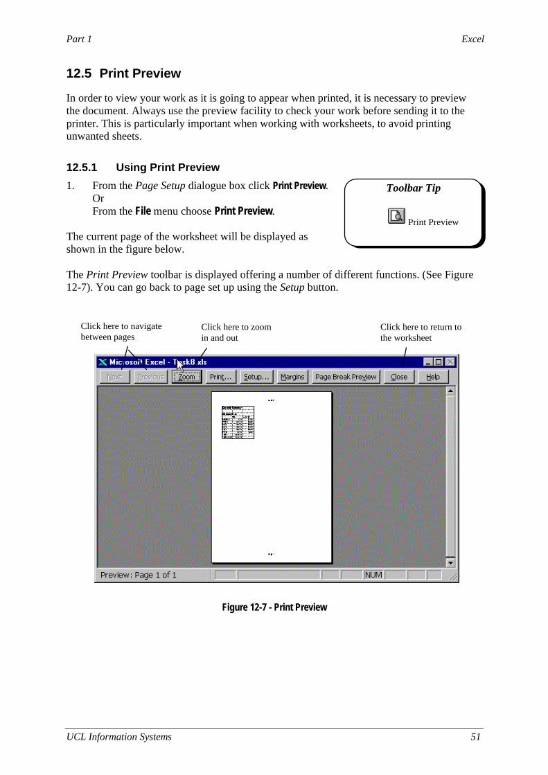
12.5 Print Preview

In order to view your work as it is going to appear when printed, it is necessary to preview the document. Always use the preview facility to check your work before sending it to the printer. This is particularly important when working with worksheets, to avoid printing unwanted sheets.

12.5.1 Using Print Preview

1. From the Page Setup dialogue box click Print Preview. Or From the File menu choose Print Preview.

The current page of the worksheet will be displayed as shown in the figure below. The Print Preview toolbar is displayed offering a number of different functions. (See Figure 12-7). You can go back to page set up using the Setup button.

Figure 12-7 - Print Preview

Click here to navigate between pages

Click here to zoom in and out

Click here to return to the worksheet

Toolbar Tip

Print Preview

Excel Part 1


12.6 Printing a Worksheet

The worksheet can be printed directly from the Preview window, or from the Page Setup dialogue. 1. From the File menu choose Print.

The Print dialogue box appears as shown:

Figure 12-8 - Print Dialogue Box

12.6.1 To Print a Selected Range

You may specify the range of what you want to print in the current worksheet using the Print Range options. Print What allows you to choose how many pages to print. Print what also allows you to print a highlighted selection, alternative sheets or the entire work book.

Toolbar Tip

Print

Choose what you wish to print here

Print All or specify page range

Part 1 Excel


Task Seventeen – Preparing to Print 1. Open the file summary.xls created in the previous task.

2. Change the page orientation to Landscape.

l From the File menu choose Page Setup and select the Page tab. l Click on Landscape.

3. Centre the worksheet horizontally on the page.

l Select the Margins tab. l In the Centre on Page section click on Horizontally. l Set the top margin to 3.5cm.

4. Create a Header to display the text OPQ Enterprises Inc. Format this text using a

suitable font and insert the date. l Select the Header/Footer tab. l Click on Custom Header. l In the Left Section type the heading OPQ Enterprises Inc. l Highlight the text and click on the Font button to choose 10pt Garamond Italic. l Click in the Right Section box and click the Date button to insert today’s date. l Format the date using Garamond Italic 10pt as before. l Create a Footer to display your name and the filename. Format these using the

same format as for the Header. 5. Choose the print option to display the Row and Column headings.

l Choose the Sheet tab and click in the Row and column headings box. 6. View your worksheet in Print Preview. When you are satisfied print the entire

worksheet. 7. Now select the range A2:B10 in the worksheet.

8. Print the selection (from the Print dialogue box choose Selection in the Print what

box). 9. Save the file with the same name summary.xls and close the file.

You are now ready to try Exercises 11, 12 and 13.

Excel Part 1


13. Exercises

Training Files If you wish to attempt the following exercises and you are not using a training account it is necessary to download the training files used in this workbook from the IS training web site at: http://www.ucl.ac.uk/is/training/exercises.htm Full instructions on how to do this are provided on this web page. The downloaded files will be copied to a folder on the r:\ drive (unless other wise specified) into the r:\training.dir\excelp1 folder. Exercise 1 – Holiday Costs 1. Create a new worksheet as shown below 2. Enter a formula in cell B8 to calculate the Sub Total of the Travel Costs. When you have

entered this formula and are confident that it is correct, copy the formula to the other cells in the row (i.e. cells C8:F8).

3. Enter a formula in cell B16 to calculate the Sub Total of the Additional Costs. Copy this

formula to cells C16:F16. 4. Enter a formula in cell B18 to calculate the Grand Total. Copy this formula to cells

C18:F18. 5. Save the file as holiday.xls in the r:\training.dir\excelp1 folder.

Part 1 Excel


Exercise 2 – Newspaper Sales 1. Open the workbook news.xls

This worksheet shows details of the volume of different newspapers sold over a period of 15 weeks together with the retail price of each of the newspapers available.

2. To improve the layout of the worksheet insert a row between rows 9 and 10.

3. The data for Weeks 3 and 4 has been duplicated in error. Delete these two extra rows (i.e. rows 15 and 16).

4. Enter a formula to add up the number of Newspapers Sold over the 15 weeks.

• In cell B27 use the AutoSum button. • In cell C27 try typing the formula manually.

Check that the formula is correct and then copy it to the remaining columns.

5. Enter a formula in cell B28 to calculate the Total Sales using the retail prices given. Total Sales = Newspapers Sold * Retail Price (Note: make sure you use the appropriate retail price for each newspaper). Hint: If you are unclear how to create this formula, try substituting the relevant cell references into the formula exactly as it is given. For example, to calculate the Total Sales of The Chronicle use the formula:

Total Sales = Newspapers Sold * Retail Price becomes: = B27 * B3

6. Copy the formula in cell B28 to cell C28. What happens? (Check the formula in cell C28).

7. Manually enter the correct formula into each of the cells C28:H28.

8. Save the worksheet with the new name news1.xls and close the file.

9. How would you consider changing the layout of this worksheet so that all formula could be copied automatically?

Excel Part 1


Exercise 3 – Newspaper Sales 1. Open the workbook news1.xls that you created in a previous exercise.

2. Some simple statistical analysis (i.e. the average, minimum and maximum sales) is

required for each of the newspapers. Insert the labels: Average Minimum Maximum after the Total Sales label in rows 30, 31 and 32.

3. Enter a formula to calculate the Average, Min and Max values for each of the different Newspapers. Try: • using the function wizard • typing the formula yourself

(Take care not to include the calculated values Newspapers Sold and Total Sales.

4. Using the function wizard find for yourself a suitable function to automatically return the current date insert this function in cell H1.

5. Save the worksheet as news2.xls and close it. Formatting Data Exercise 4 – Number Formats - Holiday Costs

1. Open the worksheet holiday.xls which you created in a previous exercise.

2. Format all the columns to a Currency format with two decimal places. Try using the Currency button.

3. Format the Sub Total rows (row 8 and 16) to a Number format with one decimal place.

4. Format the Grand Total row to a Currency format with no decimal places.

5. Change the width of Column A to approximately width:18.00.

6. Save the worksheet with the new name holiday1.xls

Part 1 Excel


Exercise 5 – Number Formats - Newspaper Sales 1. Open the worksheet news2.xls which you created in a previous exercise.

2. Format the Total Sales row to a Currency format with two decimal places. Try using

the Currency button.

3. Format the Average row to an integer (i.e. no decimal places). Try using the Format menu.

4. Format the Date Value (cell H1) to dd-mmm-yy e.g. 04-Mar-97 format.

5. Change the width of column A to width 20.00 and the width of columns B, C, D, and E using Best Fit – AutoFit. Try changing the width of all four columns together in one operation.

6. Save the worksheet with the new name news3.xls. Exercise 6 – Character Formats - Holiday Costs 1. Open the worksheet holiday1.xls which you created in a previous exercise.

In this exercise we are going to apply further formatting to the worksheet.

2. Centre the title Holiday Costs across the top of the worksheet. Increase the size to 16 points.

3. Embolden and right align all the column headings.

4. Embolden the Sub Total and Grand total labels.

5. Add a bottom border under the country labels i.e. cells B2:F2 and add a double bottom

border to the Grand Total figures in cells B18:F18.

6. Save the worksheet with the same name, holiday1.xls.

Excel Part 1


Exercise 7 – More Formatting – Newspaper Sales 1. Open the worksheet news3.xls that you created in a previous exercise.

2. Insert a row at the top of the worksheet and insert the title The Paper Shop. Centre this

title across the top of the worksheet. Format this to AvantGarde 18pt.

3. Embolden and right align all the column headings.

4. Embolden the row labels Week1, Week2 etc.

5. Add top and bottom borders around the Sales figures i.e. cells A12:H29 and add a double border below the row Week 15 i.e. A27:H27.

6. Add shading of your choice to the Average, Minimum and Maximum rows i.e. cells A31:H33.

7. Save the worksheet with the same name, news3.xls. 8. Now use the AutoFormat facility to format the worksheet – select a style of your choice.

Experiment by selecting the entire worksheet and a single cell in the worksheet. Try applying a range of styles.

9. Close the worksheet without saving it. Page Setup and Printing Exercise 1 – Newspaper Sales 1. Open the file news3.xls you created in the previous exercise.

2. Change the Page Layout to Landscape orientation.

3. Change the Top margin to 2cm and the Left margin to 5cm. Change both the Header

and Footer margins to 0.5cm.

4. Insert a header with the title “The Paper Shop”. Format this using font type AvantGarde, bold italic at 12pt and delete the Tab field. Insert a footer with your name in the left hand corner and the filename in the right-hand corner. Format in the same style as the header, making sure you delete the Page field.

5. Remove the gridlines and view the document in Print Preview. Print and save the worksheet with the same name.

Part 1 Excel


Revision Exercises Exercise 9 – Petty Cash 1. Create a Petty Cash worksheet as shown here. Save it with the name petty.xls in the

r:\training.dir\excelp1 folder.

2. Apply a currency format with two decimal places to the data where appropriate. 3. Insert a row between rows 1 and 2 and remove the blank row 4. 4. Enter formulae to calculate the Weekly Total for each of the weeks. 5. Week 3 has been omitted in error. Insert a row and add the following data:

Milk Postage Stationery Week3 3.00 4.00 5.00

6. Copy the formula to this row.

7. Enter the formula to calculate the Monthly Total for each item. 8. During some weeks coffee is also purchased.

Insert a new column between Milk and Postage, and enter the heading Coffee, with the following data:

9. Copy the formulae for this column. 10. You have been asked to give a rough estimate of the total yearly outgoing of petty cash.

Insert a new label below Monthly Total called Yearly Estimate. Insert a formula in cell B9 to multiply the Monthly Total for Milk by 12. Copy this formula across the remainder of the cells in this row.

11. Enter a label Grand Total in cell A10. Now sum the Yearly Estimate row to calculate the

grand total for the year. Place this total in cell B10. 12. Format the font to Comic Sans MS 12pt. 13. Embolden the text in the row and column headings.

Coffee Week1 4.30 Week2 3.50 Week3 0 Week4 5.20

Excel Part 1


14. Set the width of each column to approximately width:12.00.

15. Format the text in column A so that it wraps within the cells. 16. . Centre the heading across columns A to F. 17. Add a heavy border around the outside of the table - apart from the heading i.e. A3:F10.

Add horizontal lines between the rows containing the summary data (Monthly Total, Yearly Estimate and Grand Total).

18. Add a header to the worksheet to include the filename in the centre portion. Add a footer

to include the date on the right, and your name on the left. 19. Centre the data both vertically and horizontally on the page, for printing.

20. Select to print Row and Column headings. 21. Print the worksheet and save it with the same name, petty.xls Exercise 9 – Confectionery Sales 1. Create a worksheet as shown below to record confectionery sales in the student refectory.

The prices are given in British pounds.

Items Price Number Sold Total Sold Sales Week 1 Week 2 Week 3 Week 4 Mars Bar 0.29 55 72 65 70 Formula Formula Snicker 0.32 38 62 44 59 Formula Formula Fuse 0.30 122 54 98 84 Formula Formula KitKat 0.29 98 115 90 101 Formula Formula Bounty 0.34 65 83 65 79 Formula Formula Wispa 0.31 48 52 35 67 Formula Formula Total Sold per Week

Formula Formula Formula Formula Formula Formula

2. Save the worksheet as sweets.xls in the r:\training.dir\excelp1 folder.

3. Create a formula in the Total Sold column to calculate the total of each type of bar sold.

Total Sold = number sold in week 1 + number sold in week 2 + number sold in week 3 + number sold in week 4

4. Create a formula in the Sales column to calculate the sales value of each type of chocolate bar sold. Sales = Total Sold * Price

5. In the row Total Sold per Week, create a formula to calculate the total number of

chocolate bars sold per week. Total Sold per Week = Mars Bars + Snickers + Fuse + KitKat + Bounty + Wispa

6. Add two new rows at the bottom of the worksheet and label these Minimum Sold and Maximum Sold. Create formulae in these rows to calculate the Minimum chocolate bars

Part 1 Excel


sold per week and the Maximum chocolate bars sold per week.

7. Format the figures in the column Price to currency with two decimal places and the figures in the column Sales as integer (no decimals). Embolden all column titles.

8. Add one column to the right of the table, with the title: "Sales in Euros".

9. Using the exchange rate 1 GBP = 0.60 EURO. (The prices shown in the worksheet are expressed in GBP). Create a formula to calculate Sales in EMU for each chocolate bar in the column. Sales in EMU = Sales * Exchange Rate (0.6)

10. Create a header with the text: College Confectionery Sales. 11. Print a copy of the worksheet and Save the worksheet with the same name, sweets.xls

ECDL Module 4 - UCL HEP Group · ECDL: Module 4 Spreadsheets ... (ECDL) Excel 2002 Part 1 is the...

Documents

Transcript of ECDL Module 4 - UCL HEP Group · ECDL: Module 4 Spreadsheets ... (ECDL) Excel 2002 Part 1 is the...