Astronomy&Astrophysics

A&A 629, A125 (2019)https://doi.org/10.1051/0004-6361/201935682© J. Wicht et al. 2019

Dynamo action of the zonal winds in JupiterJ. Wicht1, T. Gastine2, L. D. V. Duarte3, and W. Dietrich1

1 Max Planck Institute for Solar System Research, Justus-von-Liebig-Weg 3, 37077 Göttingen, Germanye-mail: wicht@mps.mpg.de

2 IPGP, Institut de Physique du Globe de Paris, Sorbonne Paris Cité, Université Paris-Diderot, UMR 7154 CNRS, 1 rue Jussieu,75005 Paris, France

3 College of Engineering, Mathematics and Physical Sciences, University of Exeter, Physics building, Stocker Road, Exeter,EX4 4QL, UK

Received 12 April 2019 / Accepted 5 July 2019

ABSTRACT

The new data delivered by NASA’s Juno spacecraft significantly increase our understanding of the internal dynamics of Jupiter. Thegravity data constrain the depth of the zonal flows observed at cloud level and suggest that they slow down considerably at a depth ofabout 0.96 rJ, where rJ is the mean radius at the one bar level. The magnetometer onboard Juno reveals the internal magnetic field of theplanet. We combine the new zonal flow and magnetic field models with an updated electrical conductivity profile to assess the zonal-wind-induced dynamo action, concentrating on the outer part of the molecular hydrogen region of Jupiter where the conductivityincreases very rapidly with depth. Dynamo action remains quasi-stationary and can therefore reasonably be estimated where themagnetic Reynolds number remains smaller than one, which is roughly the region above 0.96 rJ. We calculate that the locally inducedradial magnetic field reaches rms values of about 10−6 T in this region and may just be detectable by the Juno mission. Very localizeddynamo action and a distinct pattern that reflects the zonal wind system increases the chance to disentangle this locally induced fieldfrom the background field. The estimates of the locally induced currents also allow calculation of the zonal-flow-related Ohmic heatingand associated entropy production. The respective quantities remain below new revised predictions for the total dissipative heating andtotal entropy production in Jupiter for any of the explored model combinations. Thus, neither Ohmic heating nor entropy productionoffer additional constraints on the depth of the zonal winds.

Key words. planets and satellites: magnetic fields – planets and satellites: gaseous planets – magnetohydrodynamics (MHD) –dynamo

1. Introduction

Two of the main objectives of NASA’s Juno mission are to mea-sure the magnetic field of Jupiter with unprecedented resolutionand to determine the depth of the fierce zonal winds observedin its cloud layer. The first Juno-based internal magnetic fieldmodel JRM09 (Connerney et al. 2018) already provides the inter-nal magnetic field up to spherical harmonic degree 10 and showsseveral interesting features that seem unique to the dynamo ofJupiter (Moore et al. 2018). Better-resolved models are expectedas the mission continues.

Based on Juno gravity measurements (Iess et al. 2018), Kaspiet al. (2018) deduce that the speed of the equatorially antisym-metric zonal flow contributions must be significantly reduced ata depth of about 3000 km below the one-bar level, which corre-sponds to a radius of 0.96 rJ. Kong et al. (2018) come to roughlysimilar conclusions with a different inversion procedure, but theyalso point out that the solution is not unique. While the gravitydata only allow us to constrain the equatorially antisymmetricwinds, the results likely also extend to the symmetric contri-butions. New interior models (Guillot et al. 2018; Debras &Chabrier 2019) and also the width of the dominant equatorialjet (Gastine et al. 2014; Heimpel et al. 2016) both support theidea that the fast zonal winds are roughly confined to the outer4% in radius.

The fast planetary rotation enforces geostrophic flow struc-tures with minimal variation along the direction of the rotation

axis. Geostrophic zonal winds are therefore expected to reachright through the gaseous envelope of the planet, and it remainsunclear which mechanism limits their extent in Jupiter. Thedemixing of hydrogen and helium and the subsequent precip-itation of helium deeper into the planet offers one possibleexplanation (Militzer et al. 2016). This process would have estab-lished a helium gradient that suppresses convection. In Jupiter,this stable helium-rain layer may start somewhere between 0.93and 0.90 rJ and perhaps extends down to 0.80 rJ (Debras &Chabrier 2019). We note however that ab initio simulations bySchöttler & Redmer (2018) predict that the hydrogen/heliumdemixing may not even have started. Recent analysis of gravitymeasurements by the Cassini spacecraft suggest that the zonalwinds of Saturn may only reach down to about 0.85 rS (Iesset al. 2019; Galanti et al. 2019). Since the stably stratified layeris thought to start significantly deeper, at about 0.62 rS accord-ing to Schöttler & Redmer (2018), it cannot be the reason for thelimited depth of the zonal winds.

A second possible mechanism braking of the zonal windsat depth involves the Lorentz forces. Lorentz forces are tied todynamo action and thus to the electrical conductivity profile. Abinitio simulations for Jupiter suggest that ionization effects leadto a super-exponential increase of the electrical conductivity inthe outermost molecular gas envelope. We refer to this layer asthe Steeply Decaying Conductivity Region (SDCR) of Jupiterin the following. At about 0.9 rJ, hydrogen, the main constituentof the planet, becomes metallic, and the conductivity increases

A125, page 1 of 11Open Access article, published by EDP Sciences, under the terms of the Creative Commons Attribution License (http://creativecommons.org/licenses/by/4.0),

which permits unrestricted use, distribution, and reproduction in any medium, provided the original work is properly cited.Open Access funding provided by Max Planck Society.

A&A 629, A125 (2019)

0.80 0.82 0.84 0.88 0.90 0.92 0.94 0.98 1.000.86 0.96

105

100

10-5

r/rJ

��(S

/m)

French et al. (2012)

�F

�Z

Zaghoo & Collins (2018)

Nellis et al. (1996)

Liu et al. (2008)

0.80 0.82 0.84 0.88 0.90 0.92 0.94 0.98 1.000.86 0.96

r/rJ

10-1

10-2

10-3

10-4

D�/

r J

�F

�Z

a)

b)

Fig. 1. Panel a: electrical conductivity profiles in the outer 20% of theradius of Jupiter. The black line shows the parametrization σF(r) of theab initio simulation data points (black circles) by French et al. (2012).The dotted red line shows the profile published in Zaghoo & Collins(2018), while the solid red line shows the extension σZ(r) used here. Theprofiles suggested by Liu et al. (2008) (green) and Nellis et al. (1999)(blue) are shown for comparison. Panel b: magnetic diffusivity scaleheight Dλ/rJ for σF and σZ .

much more smoothly with depth (French et al. 2012); see panela of Fig. 1. Though dynamo action and the potential braking ofthe zonal winds due to Lorentz forces are classically attributed tothe metallic region, they may already become significant wherethe electrical conductivity reaches sizable levels in the SDCR ofJupiter.

Different dynamo-related arguments have been evoked toestimate the depth of the zonal winds without however directlyaddressing the role of the Lorentz forces. Liu et al. (2008)estimate that the Ohmic heating caused by zonal-wind-relatedinduction would exceed the total heat emitted from Jupiter’sinterior should the winds reach deeper than 0.96 rJ with undi-minished speed. Ridley & Holme (2016) argue that the secularvariation of the magnetic field over 30 yr of pre-Juno obser-vations is relatively small and is thus likely incompatible withan advection by undiminished zonal winds. These latter authorsconclude that the winds cannot reach depths where the magneticReynolds number exceeds one and more significant inductioncan be expected. This puts the maximum depth somewherebetween 0.96 rJ and 0.97 rJ, as we discuss below. A recent

analysis by Moore et al. (2019) suggests that the observationsover a 45 yr time-span, including Juno data, would be compati-ble with zonal wind velocities of 2.4 m/s at 0.95 rJ, two orders ofmagnitude lower than observed in the cloud layer.

Another interesting question is how much the dynamo actionin the SDCR of Jupiter contributes to the total magnetic field.Using a simplified mean-field approach, Cao & Stevenson (2017)predict that the radial component of the locally induced field(LIF) may reach 1% of the background field and could there-fore be detectable by the Juno magnetometer. Wicht et al. (2019)analyze the dynamo action in the SDCR of fully self-consistentnumerical simulations that yield Jupiter-like magnetic fields.Because of the dominance of Ohmic diffusion, the dynamodynamics becomes quasi-stationary in the SDCR of their simula-tions. A consequence is that the locally induced electric currentsand field can be estimated with relatively good precision whenflow, electrical conductivity profile, and the surface magneticfield are known. The new constraints on the internal magneticfield of Jupiter and the depth of the zonal winds provided bythe Juno mission, combined with improved estimates on theelectrical conductivity profile, allow a fresh look at the problem.

Here we use three different zonal flow models, two electri-cal conductivity models, and the new Juno-based magnetic fieldmodel JRM09 to predict the electric currents and magnetic fieldsproduced in the SDCR of Jupiter. In addition, we also derivenew estimates for the total dissipative heating and related entropyproduction and explore whether either value is exceeded by thezonal-flow-related Ohmic dissipation.

Section 2 outlines the methods and introduces the data weused. Section 3 discusses dissipative heating and entropy pro-duction in Jupiter. Estimates for dynamo action, Ohmic heating,and entropy production are then presented in Sect. 4. Section 5closes the article with a discussion and conclusion.

2. Methods and data

2.1. Estimating dynamo action

The ratio of inductive to diffusive effects in the inductionequation,

∂B∂t

= ∇ × (U × B) − ∇ × λ∇ × B, (1)

can be quantified by the magnetic Reynolds number

Rm =〈U〉 Dλ

, (2)

where λ = 1/(µσ) is the magnetic diffusivity, with µ the mag-netic permeability and σ the electrical conductivity. Angularbrackets generally denote rms values at a given radius throughoutthe paper; thus 〈U〉 stands for

〈U〉 =

(1

4π

∫ 2π

0dφ

∫ π

0dθ sin θ U2

)1/2

, (3)

with θ being the colatitude and φ the longitude.The typical length scale D is hard to estimate, and the plane-

tary radius is often used for simplicity. Sinceσ decreases steeplyin the SDCR, the length scale is determined by the conductivityor magnetic diffusivity scale height:

Dλ =λ

∂λ/∂r= − σ

∂σ/∂r, (4)

A125, page 2 of 11

J. Wicht et al.: Dynamo action of the zonal winds in Jupiter

and the modified magnetic Reynolds number,

Rm(1) =〈U〉 Dλ

λ(5)

should be used. Since Dλ is small and λ decreases steeply withradius, most of the SDCR of Jupiter is characterized by a smallmagnetic Reynolds number Rm(1) < 1, and the magnetic fielddynamics becomes quasi-stationary (Liu et al. 2008), obeyingthe simplified induction equation

∇ × jσ≈ ∇ × (U × B̃). (6)

Here, j is the current density and B̃ the strong backgroundfield produced by the dynamo acting deeper in the planet. TheLIF B̂ is given by Ampere’s law:

j = ∇ × B̂/µ. (7)

The steep σ profile dominates the radial dependence of j andB̂ in the SDCR. The current density is thus dominated by thehorizontal components, where radial gradients in B̂ contribute(Liu et al. 2008; Wicht et al. 2018):

j ≈ jH ≈ r̂ × ∂

∂rB̂H . (8)

Index H denotes the horizontal components; the radial cur-rent can be neglected in comparison.

Along the same lines, the horizontal components of Eq. (6)can be approximated by

1r∂

∂rrσ

jH ≈ −r̂ × [∇ × (U × B̃)]H , (9)

where r̂ is the radial unit vector. Integration in radius yields theintegral current density estimate introduced by Liu et al. (2008),which we identify with an upper index (I):

j(I)H =

σ

r

[ rσ

jH

]

rJ

+ r̂ × σr

∫ rJ

rdr′ r′ [∇ × (U × B̃)]H . (10)

The square brackets with a lower index rJ indicate that theexpression should be evaluated at the outer boundary.

For a predominantly zonal flow, we can use the approxima-tion[∇ ×

(U × B̃

)]H≈ − Uφ

r sin θ

(∂

∂φB̃θ

)θ̂

+1r

[∂

∂r

(rUφB̃r

)+∂

∂θ

(UφB̃θ

)]φ̂, (11)

where Uφ is the zonal flow component and θ̂ and φ̂ are unitvectors in latitudinal and azimuthal direction, respectively.

The integral estimates for the two horizontal current compo-nents are then given by

j(I)θ =

σ

r

[ rσ

jθ]

rJ

− σr

([r UφB̃r

]rJ−

[r UφB̃r

]r

)

− σ

r

∫ rJ

rdr′

∂

∂θ(UφB̃θ), (12)

and

j(I)φ =

σ

r

[ rσ

jφ]

rJ

− σr

∫ rJ

rdr′

Uφ

sin θ∂

∂φB̃θ. (13)

Since the latitudinal length scale of the zonal winds issmaller than the azimuthal length scale of the magnetic field,we expect that the latitudinal component dominates.

The integral estimate requires the knowledge of the surfacecurrents. While the surface currents are certainly very small, thescaled version σ(r)/σ(rJ) j may remain significant. Liu et al.(2008) argue that neglecting the surface contribution at leastprovides a lower bound for the rms current density.

Wicht et al. (2019) confirm that the dynamics indeedbecomes quasi-stationary in the SDCR of their Jupiter-likedynamo simulations and that jθ is indeed the dominant currentcomponent where Rm(1) < 1. They also report that the simplifiedOhm’s law for a fast-moving conductor,

j(O) = σ(U × B̃), (14)

provides a significantly better estimate than j(I). We identify therespective current estimate with an upper index (O). The generalOhm law,

j = σ (U × B + E) , (15)

also contains currents driven by the electric field, which reducesto E = −∇Φ in the quasi-stationary case, where Φ is the elec-tric potential. In the SDCR of Jupiter, this contribution likelyproves secondary because the potential differences remain smallcompared to the induction by fast zonal winds (Wicht et al.2019).

As the electrical conductivity decreases in the SDCR, themagnetic field approaches a potential field with its characteristicradial dependence. We use this dependence to approximate thebackground field with

B̃`(r, θ, φ) ≈( rJ

r

)`+2B`(rJ , θ, φ), (16)

where the index ` denotes the magnetic field contribution atspherical harmonic degree `. This provides a suitable approxi-mation as long as the LIF remains a small contribution of thetotal field (Wicht et al. 2019).

Given a surface field model and an electrical conductivityprofile, Ohm’s law for a fast moving conductor and a predomi-nantly zonal flow suggests

j ≈ j(O)θ θ̂ = σ Uφ B̃r θ̂. (17)

When using this result to constrain the outer-boundary cur-rents, the alternative integral estimates, Eqs. (12) and (13), yield

j(I)θ = σ Uφ B̃r − σ

r

∫ rJ

rdr′

∂

∂θ(UφB̃θ) (18)

and

j(I)φ = −σ

r

∫ rJ

rdr′

Uφ

sin θ∂

∂φB̃θ, (19)

respectively. A comparison of the estimates shows that j(I) andj(O) will remain very similar at shallow depths. When the flowdecays very deeply with depth however, the integral contribu-tions in Eqs. (18) and (19) dominate below some radius and causelarger deviations, as we show below.

Calculating the LIF requires to uncurl Ampere’s law, whichreduces to integrating Eq. (8) in the SDCR of Jupiter. When

A125, page 3 of 11

A&A 629, A125 (2019)

using j(O), this yields

B̂H ≈∫ rJ

rdr′

r̂ × (U × B̃)λ

. (20)

Since the electrical conductivity profile rules the radialdependence, the integral can be approximated by

B̂H ≈ Dλ

λr̂ × (U × B̃). (21)

We assume here that the LIF vanishes at the outer boundary.For a dominantly azimuthal flow, the primary LIF component isalso azimuthal:

B̂φ ≈ Dλ

λUφB̃r. (22)

This suggests that the rms value scales with Rm(1),

〈B̂H〉 ≈ Rm(1)〈B̃〉, (23)

assuming that the correlation between Uφ and B̃r is of littlerelevance.

The radial LIF can be estimated based on the radial compo-nent on the quasi-stationary induction Eq. (1):

λ∇2B̂r ≈ −r̂ · ∇ × (U × B̃). (24)

When approximating Ohmic dissipation by λB̂r/D2λ, this

yields:

B̂r ≈ −D2λ

λr̂ · ∇ × (U × B̃), (25)

which reduces to

B̂r ≈ −D2λ

λ

Uφ

r sin θ∂

∂φB̃r (26)

for a predominantly zonal flow. This suggest that the rms radialLIF should roughly scale with the second modified magneticReynolds number

Rm(2) =〈U〉 D2

λ

λ D(27)

like

〈B̂r〉 ≈ Rm(2) DDφ〈B̃〉. (28)

Here, Dφ is the azimuthal length scale of the backgroundfield. Since Dλ � Dφ, the radial LIF is much smaller than itshorizontal counterpart (Wicht et al. 2019).

2.2. Data

The electric current and LIF estimates discussed above requirea conductivity profile, a zonal flow model, and a surface mag-netic field model. For the heating and entropy estimates that wederived in Sect. 3, we also need density, temperature, and ther-mal conductivity profiles. We adopt the interior model calculatedby Nettelmann et al. (2012) and French et al. (2012), which isthe only one that provides all the required information. We notehowever that recent Juno gravity data suggest that the interior

of Jupiter may be more complex than anticipated in this model(Debras & Chabrier 2019).

Ab initio simulations of the electrical conductivity by Frenchet al. (2012) provide 12 data points at different depths. Figure 1shows the values in the outer 20% of the radius of Jupiter andthe parametrization σF(r) developed for our analysis. A linearbranch,

σF(r) = σr + (σm − σr)r − rr

rm − rr, (29)

covers the smoother inner part r < rm. An exponential branch,

σF(r) = σm exp

r − rm

rm − rr+ b

(r − rm

rm − rr

)2σm − σr

σm

, (30)

describes the steeper decay for rm < r < re with b = 7.2. Match-ing radius rm = 0.89 rJ and reference radius rr = 0.77 rJ arechosen where ab initio data points have been provided.

A double-exponential branch,

σF(r) = σe exp(d

[exp

(c

r − re

rm − rr

)− 1

]), (31)

is required to capture the super-exponential decrease for r ≥ re =0.972 rJ. The additional free parameter is c = 10, while σe =σ(re) and

d =1c

(1 + 2 b

re − rm

rm − ri

)σm − σr

σm. (32)

The dotted red line in panel a of Fig. 1 shows the con-ductivity model used to study dynamo action in Jupiter andJupiter-like exoplanets by Zaghoo & Collins (2018). This is basedon measurements which suggest a higher electrical conductivityin the metallic hydrogen phase than previous data. Unfortunately,Zaghoo & Collins (2018) do not discuss how the results wereextrapolated to Jovian conditions. The solid red line in Fig. 1shows the respective parametrization σZ(r) used for our analysis,which retraces the published curve and connects to previouslypublished parametrizations (green and blue) at lower densities(Nellis et al. 1996; Liu et al. 2008). We note however that theseparametrizations are based on data (Weir et al. 1996) which mayhave been attributed to overly low temperatures according to arecent analysis by Knudson et al. (2018).

Though model σZ(r) is somewhat arbitrary, it serves toillustrate the impact of conductivity uncertainties in our study.Close to rJ where conductivities remain insignificant, σF ismany orders of magnitude larger than σZ . The ratio σF/σZdecreases with depth, reaching 102 around 0.97 rJ and 10 around0.96 rJ. The two models finally cross at about 0.95 rJ. At about0.925 rJ, the ratio reaches a minimum of 0.05 and then slowlyincreases with depth to 0.35 at 0.8 rJ. Table 1 list values of bothconductivity models for selected radii.

Panel b of Fig. 1 and selected values listed in Table 1 demon-strate that the magnetic diffusivity scale heights Dλ differ muchless than the conductivities themselves. Electric currents, LIFs,and Ohmic heating depend linearly on σ but on different powersof Dλ. The differences between the results for the two conductiv-ity models is therefore predominantly determined by σ and caneasily be scaled from one to the other.

The three different zonal flow models explored here are illus-trated in Fig. 2. Table 1 lists rms values 〈Uφ〉 at selected radii. Allreproduce the observed zonal winds at r = rJ (Porco et al. 2003;

A125, page 4 of 11

J. Wicht et al.: Dynamo action of the zonal winds in Jupiter

Table 1. Rms flow velocities, electrical conductivities σ, magnetic diffusivities λ, diffusivity scale heights Dλ, and magnetic Reynolds numbersRm(1) at selected radii.

r/rJ 0.98 0.97 0.96 0.95 0.94 0.92 0.90

〈UG〉 (m s−1) 3.0× 101 3.2× 101 3.5× 101 3.8× 101 4.1× 101 2.5× 101 1.5× 101

〈UK〉 (m s−1) 2.0× 101 1.4× 101 8.0× 100 4.0× 100 2.0× 100 2.5× 10−1 4.0× 10−2

〈UZ〉 (m s−1) 2.3× 101 1.9× 101 1.5× 101 1.1× 101 6.8× 100 1.7× 100 2.4× 10−1

σF (S m−1) 3.2× 10−4 3.7× 10−2 9.7× 10−1 1.7× 101 2.1× 102 9.3× 103 8.6× 104

σZ (S m−1) 1.5× 10−8 1.9× 10−4 1.6× 10−1 3.4× 101 2.0× 103 1.5× 105 3.9× 105

λF (m s−2) 2.5× 109 2.2× 107 8.2× 105 4.6× 104 3.8× 103 8.5× 101 9.2× 100

λZ (m s−2) 5.2× 1013 4.1× 109 5.1× 106 2.3× 104 3.9× 102 5.5× 100 2.0× 100

Dλ(σF)/rJ 1.4× 10−3 2.9× 10−3 3.2× 10−3 3.7× 10−3 4.4× 10−3 6.6× 10−3 1.4× 10−2

Dλ(σZ)/rJ 7.9× 10−4 1.4× 10−3 1.7× 10−3 2.1× 10−3 2.9× 10−3 1.2× 10−2 3.3× 10−1

Rm(1)(UG, σF) 1.2× 10−3 2.9× 10−1 9.6× 100 2.1× 102 3.2× 103 1.4× 105 1.5× 106

Rm(1)(UK , σF) 8.2× 10−4 1.3× 10−1 2.2× 100 2.3× 101 1.6× 102 1.4× 103 4.2× 103

Rm(1)(UZ , σF) 9.1× 10−4 1.8× 10−1 4.2× 100 6.2× 101 5.4× 102 9.3× 103 2.6× 104

Rm(1)(UG, σF) 3.2× 10−8 7.4× 10−4 7.9× 10−1 2.4× 102 2.1× 104 3.8× 106 1.6× 107

Rm(1)(UK , σF) 2.2× 10−8 3.2× 10−4 1.8× 10−1 2.5× 101 1.0× 103 3.9× 104 4.3× 104

Rm(1)(UZ , σF) 2.4× 10−8 4.5× 10−4 3.4× 10−1 6.9× 101 3.5× 103 2.7× 105 2.7× 105

Vasavada & Showman 2005). We use a running average of thesurface profile with a window width of one degree and representthe result with 256 (nearly) evenly spaced latitudinal grid pointsfor our calculations.

The three flow models differ at depth. The most simple one,UG, assumes geostrophy in each hemisphere, that is, the flowdepends only on the distance s = r sin θ to the rotation axis.Kaspi et al. (2018) describe the depth decay of the equatoriallyantisymmetric zonal flow with profiles constrained by the Junogravity measurements. We apply their “latitude-independent”model version to the total zonal flow and refer to this modelas UK . The rms amplitude of UK has decreased by one orderof magnitude at about 0.95 rJ and by two orders of magnitudearound 0.925 rJ.

We also consider the “deep” model suggested by Konget al. (2018), who assume an exponential depth decay and anadditional linear dependence on the distance z = cos θ to theequatorial plane. Like for UK , our respective model UZ assumesthat the depth and z dependences, which were originally derivedfor the equatorially antisymmetric contributions, apply to thewhole flow. The rms velocity in UZ decays more smoothly withdepth than in UK , having decreased by one order of magnitude atabout 0.935 rJ and by two orders of magnitude at about 0.905 rJ.

Figure 2 shows that UG and UK have discontinuities at theequatorial plane. These pose a problem when calculating the lat-itudinal zonal flow derivatives required for the integral estimatej(I)θ (see Eq. (18)). Formally, the derivative becomes infinite at

the equator. Practically however, the impact of the discontinu-ity depends on the model setup and on the methods used forcalculating the derivatives. We tested the impact on rms cur-rent density estimates by comparing calculations covering alllatitudes with counterparts where the derivatives were explic-itly set to zero in a six-degree belt around the equator. Simplefirst-order finite differences with 256 grid points at each radiallevel are generally used for calculating the derivative. For flowUZ , which has been constructed to avoid the discontinuity (Konget al. 2018), the belt contributes not more than one percent to〈 j(I)θ 〉 at any radius, which is less than the surface fraction it

represents. For flow UK , the contribution is even smaller due tothe faster decay of the flow amplitude. However, for UG the beltcontributes 20% to the rms current for radii below 0.94 rJ, whichis a clear sign that the unphysical discontinuity causes problems.We take a conservative approach and only consider flow modelUZ in connection with estimate j(I)

θ below.The radius where Rm(1) = 1, which we refer to as r1 in the

following, roughly marks the point where the approximationsdiscussed above break down (Wicht et al. 2019). Figure 3a illus-trates the Rm(1) profiles that result from combining σF and σZwith rms values for the three zonal flow models. Table 1 com-pares values at some selected radii. These modified magneticReynolds numbers exceed unity between r1 = 0.957 rJ for thecombination σZ and UK and r1 = 0.967 rJ for σF and UG. All r1values are listed in Table 2.

Green lines in Fig. 3 show Rm(1) profiles for a typical con-vective velocity of 10 cm s−1 suggested by scaling laws (e.g., seeDuarte et al. 2018). Numerical simulations show that the velocityincreases with radius, an effect not taken into account here. Thecomparison of the different Rm(1) profiles suggests that zonal-flow-related dynamo action should dominate at least in the outer9% in radius.

For the surface magnetic field of Jupiter we use the JRM09model by Connerney et al. (2018), which provides information upto spherical harmonic degree ` = 10. The more recent model byMoore et al. (2018) is only slightly different. In order to check theimpact of smaller-scale contributions, we also tested the numer-ical model G14 by Gastine et al. (2014), which reproduces thelarge-scale field of Jupiter and provides harmonics up to ` = 426.Since it turned out that the impact of the smaller scales is verymarginal, the results are not shown here.

3. Dissipative heating and entropy production inJupiter

Liu et al. (2008) constrain the depth of the zonal winds byassuming that the related total Ohmic heating should not exceedthe heat flux out of the planet. Unfortunately, this assumption is

A125, page 5 of 11

A&A 629, A125 (2019)

0 18020 160140120100806040

colatitude

1.00

0.90

0.98

0.96

0.94

0.92

1.00

0.90

0.98

0.96

0.94

0.92

1.00

0.90

0.98

0.96

0.94

0.92

r/r J

r/r J

r/r J

UG

-100 -50 0 50 100U [m/s]

UK

UZ

Fig. 2. Zonal flow models used in this study. Prograde flows are shownin red and yellow, while blue indicates retrograde directions.

105

100

10-5

10-10

Rm(1)

r/rJ

0.90 0.92 1.000.94 0.98

�F�Z

0.9670.965

0.963

0.9600.958

0.957

UKUZ

UG

Uc

Fig. 3. Modified magnetic Reynolds numbers for the three zonal flowand the two conductivity models explored here. Vertical lines markthe radii r1 where Rm(1) = 1. Green lines show profiles for a typicalconvective velocity of 10 cm s−1 suggested by scaling laws.

incorrect, as we show in the following. In order to arrive at moremeaningful constraints, we start by reviewing some fundamentalconsiderations.

In a quasi-stationary state, where flow and magnetic fieldare maintained by buoyancy and induction against dissipativelosses, the conservation of energy simply states that the heatflux Qo = Q(ro) through the outer boundary is the sum of theflux Qi = Q(ri) through the inner boundary and the total internalheating H:

Qo = Qi + H. (33)

We note that neither viscous nor Ohmic heating contribute toH. Since flow and magnetic field are maintained by the heat fluxthrough the system, they cannot be counted as net heat sources(Hewitt et al. 1975; Braginsky & Roberts 1995).

When furthermore neglecting the effects of helium segrega-tion, core erosion, and planetary shrinking as potential energysources, the only remaining contribution is the slow secular cool-ing of the planet. The volumetric heat source is then given by

h = ρ̃ T̃∂S̃∂t, (34)

where the tilde indicates the hydrostatic, adiabatic backgroundstate (Braginsky & Roberts 1995). Assuming that convectionmaintains an adiabat at all times, ∂S̃ /∂t remains homogeneousthroughout the convective region and obeys (Jones 2014)

∂S̃∂t

= (Qo − Qi)/ ∫

VdV ρ̃ T̃ , (35)

where∫

V dV denotes an integration over the whole convectivevolume. We note however that the thermal evolution could bemore complex should Jupiter indeed harbor stably stratifiedregions.

In order to assess dissipative heating, one must consider thelocal heat equation

ρ̃T̃(∂s∂t

+ U · ∇s)

= ∇ · (k∇T ) + h + ϕ, (36)

where ϕ denotes the volumetric dissipative heat source and k thethermal conductivity. When assuming a steady state and adopt-ing the anelastic approximation ∇ · (ρ̃U) = 0, the integration overthe shell between the inner boundary ri and radius r yields

QD(r) + QA(r) = Qi +

∫ r

ri

dr′∫

FdF

(h + ϕ + ρ̃ s Ur

∂T̃∂r

). (37)

The left-hand side is the total flux through the boundary at r,that is, the sum of the diffusive contribution,

QD(r) = −∫

FdF k

∂T∂r, (38)

and the advective contribution,

QA(r) =

∫

F(r)dF ρ̃ T̃ s Ur. (39)

The right-hand side of Eq. (37) reflects the influx throughthe lower boundary Qi plus three volumetric contributions: theslow secular cooling, the dissipative heating, and the adiabaticcooling. Writing the adiabatic cooling in terms of QA yields

A125, page 6 of 11

J. Wicht et al.: Dynamo action of the zonal winds in Jupiter

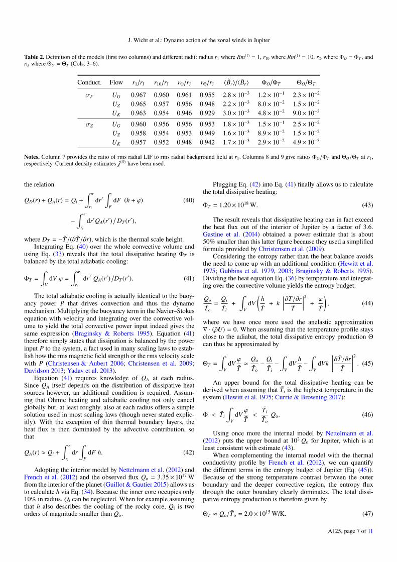
Table 2. Definition of the models (first two columns) and different radii: radius r1 where Rm(1) = 1, r10 where Rm(1) = 10, rΦ where ΦO = ΦT , andrΘ where ΘO = ΘT (Cols. 3–6).

Conduct. Flow r1/rJ r10

/rJ rΦ

/rJ rΘ

/rJ 〈B̂r〉/〈B̃r〉 ΦO

/ΦT ΘO

/ΘT

σF UG 0.967 0.960 0.961 0.955 2.8× 10−3 1.2× 10−1 2.3× 10−2

UZ 0.965 0.957 0.956 0.948 2.2× 10−3 8.0× 10−2 1.5× 10−2

UK 0.963 0.954 0.946 0.929 3.0× 10−3 4.8× 10−2 9.0× 10−3

σZ UG 0.960 0.956 0.956 0.953 1.8× 10−3 1.5× 10−1 2.5× 10−2

UZ 0.958 0.954 0.953 0.949 1.6× 10−3 8.9× 10−2 1.5× 10−2

UK 0.957 0.952 0.948 0.942 1.7× 10−3 2.9× 10−2 4.9× 10−3

Notes. Column 7 provides the ratio of rms radial LIF to rms radial background field at r1. Columns 8 and 9 give ratios ΦO/ΦT and ΘO/ΘT at r1,respectively. Current density estimates j(O) have been used.

the relation

QD(r) + QA(r) = Qi +

∫ r

ri

dr′∫

FdF (h + ϕ) (40)

−∫ r

ri

dr′QA(r′)/

DT (r′),

where DT = −T̃/(∂T̃/∂r), which is the thermal scale height.Integrating Eq. (40) over the whole convective volume and

using Eq. (33) reveals that the total dissipative heating ΦT isbalanced by the total adiabatic cooling:

ΦT =

∫

VdV ϕ =

∫ ro

ri

dr′ QA(r′)/DT (r′). (41)

The total adiabatic cooling is actually identical to the buoy-ancy power P that drives convection and thus the dynamomechanism. Multiplying the buoyancy term in the Navier–Stokesequation with velocity and integrating over the convective vol-ume to yield the total convective power input indeed gives thesame expression (Braginsky & Roberts 1995). Equation (41)therefore simply states that dissipation is balanced by the powerinput P to the system, a fact used in many scaling laws to estab-lish how the rms magnetic field strength or the rms velocity scalewith P (Christensen & Aubert 2006; Christensen et al. 2009;Davidson 2013; Yadav et al. 2013).

Equation (41) requires knowledge of QA at each radius.Since QA itself depends on the distribution of dissipative heatsources however, an additional condition is required. Assum-ing that Ohmic heating and adiabatic cooling not only cancelglobally but, at least roughly, also at each radius offers a simplesolution used in most scaling laws (though never stated explic-itly). With the exception of thin thermal boundary layers, theheat flux is then dominated by the advective contribution, sothat

QA(r) ≈ Qi +

∫ r

ri

dr∫

FdF h. (42)

Adopting the interior model by Nettelmann et al. (2012) andFrench et al. (2012) and the observed flux Qo = 3.35× 1017 Wfrom the interior of the planet (Guillot & Gautier 2015) allows usto calculate h via Eq. (34). Because the inner core occupies only10% in radius, Qi can be neglected. When for example assumingthat h also describes the cooling of the rocky core, Qi is twoorders of magnitude smaller than Qo.

Plugging Eq. (42) into Eq. (41) finally allows us to calculatethe total dissipative heating:

ΦT = 1.20× 1018 W. (43)

The result reveals that dissipative heating can in fact exceedthe heat flux out of the interior of Jupiter by a factor of 3.6.Gastine et al. (2014) obtained a power estimate that is about50% smaller than this latter figure because they used a simplifiedformula provided by Christensen et al. (2009).

Considering the entropy rather than the heat balance avoidsthe need to come up with an additional condition (Hewitt et al.1975; Gubbins et al. 1979, 2003; Braginsky & Roberts 1995).Dividing the heat equation Eq. (36) by temperature and integrat-ing over the convective volume yields the entropy budget:

Qo

T̃o=

Qi

T̃i+

∫

VdV

(hT̃

+ k∣∣∣∣∣∂T/∂r

T̃

∣∣∣∣∣2

+ϕ

T̃

), (44)

where we have once more used the anelastic approximation∇ · (ρ̃U) = 0. When assuming that the temperature profile staysclose to the adiabat, the total dissipative entropy production Θcan thus be approximated by

ΘT =

∫

VdV

ϕ

T̃≈ Qo

T̃o− Qi

T̃i−

∫

VdV

hT̃−

∫

VdVk

∣∣∣∣∣∣∂T̃/∂r

T̃

∣∣∣∣∣∣2

. (45)

An upper bound for the total dissipative heating can bederived when assuming that T̃i is the highest temperature in thesystem (Hewitt et al. 1975; Currie & Browning 2017):

Φ < T̃i

∫

VdV

ϕ

T̃<

T̃i

T̃oQo. (46)

Using once more the internal model by Nettelmann et al.(2012) puts the upper bound at 102 Qo for Jupiter, which is atleast consistent with estimate (43).

When complementing the internal model with the thermalconductivity profile by French et al. (2012), we can quantifythe different terms in the entropy budget of Jupiter (Eq. (45)).Because of the strong temperature contrast between the outerboundary and the deeper convective region, the entropy fluxthrough the outer boundary clearly dominates. The total dissi-pative entropy production is therefore given by

ΘT ≈ Qo/T̃o = 2.0× 1015 W/K. (47)

A125, page 7 of 11

A&A 629, A125 (2019)

The second-largest term in Eq. (45), the entropy due to thesecular cooling, is already two orders of magnitude smaller, at3.0× 1013 W/K. The two remaining terms, entropy flux throughthe inner boundary and the diffusive entropy flux down theadiabat, are only of order 1011 W/K.

Since the magnetic diffusivity is about 106 times larger thanits viscous counterpart in planetary dynamo regions, Ohmicheating is by far the dominating factor. We can use the currentdensity estimates to predict the Ohmic heating due to the zonalflows above radius r:

ΦO(r) =

∫ rJ

rdr′

∫

FdF

j2

σ. (48)

The conditions

ΦO(r) ≤ ΦT = 1.20× 1018 W (49)

provides a possible constraint for the depth of the zonal winds inJupiter.

The dissipative entropy production related to the Ohmicheating is given by

ΘO(r) ≈∫ rJ

rdr′

∫

FdF

j2

σ T̃. (50)

This can be used for the alternative depth constraint

ΘO(r) ≤ ΘT = 2.0× 1015 W/K. (51)

4. Dynamo action in the SDCR of Jupiter

In the following we apply the methods developed above to theSDCR of Jupiter. We first estimate the electric currents andinduced fields in Sect. 4.1 and then explore whether Ohmic heat-ing or entropy can serve to constrain the depth of the zonal windsin Sect. 4.2.

4.1. Electric currents and locally induced field

We start by discussing the current estimates for the differentzonal flow and conductivity model combinations. Figure 4acompares rms values of integral estimates j(I) and Ohm’s lawestimates j(O) for conductivity model σF and flow UZ . The inte-gral estimates of the latitudinal currents are at least 40 timeslarger than their azimuthal counterparts for all conductivity andflow model combinations. When using j(O) as outer boundarycondition for j(I) (blue line in Fig. 4), both estimates remainvery similar down to about 0.98 rJ. At 0.97 rJ however, j(I) isalready about 50% larger than j(O), and at 0.96 rJ the differ-ence has increased to about 250%. When assuming a vanishingouter boundary current for j(I), the differences are even larger:j(I) (green line) is 3.5 times larger than j(O) at 0.97 rJ and about6 times larger at 0.96 rJ.

Estimates of the rms horizontal and radial LIF are shown inFig. 4b, based on j(O) and Eq. (20) for the horizontal and onEq. (26) for the radial components. The radial LIF is betweentwo and three orders of magnitude smaller than its horizon-tal counterpart. The rougher estimates (Eqs. (23) and (28)),based on Rm(1) and Rm(2), respectively, provide values that areless than a factor two smaller and can thus safely be used fororder-of-magnitude assessments; they correctly predict that therms azimuthal LIF reaches the level of the background field atr1 and also that the ratio of radial to azimuthal LIF is about

105

100

10-5

10-15

< j > [A/m

2]

10-10

j����

j����, j�

���(rJ)=j����(rJ)

j����, j�

���(rJ)=0

j����, j�

���(rJ)=0

105

100

10-5

<B > [m

T]

a)

b)

r/rJ

0.90 0.92 0.96 1.000.94 0.98

r/rJ

0.90 0.92 0.96 1.000.94 0.98

UG

UK

UZ

Br

B�

Br

~

^

^

Fig. 4. Panel a: rms current density estimates for flow model UZ andconductivity model σF . Panel b: estimates of rms radial and horizontalLIF. The profile of 〈B̃r〉 has been included for comparison. Vertical linesmark the radii where Rm(1) = 1 for the different flow models. Currentdensity estimates j(O) and conductivity model σF have been used.

Rm(2)/Rm(1) = Dλ/rJ. At r1, the rms radial LIF is thus roughlythree orders of magnitude smaller than the background fieldor the horizontal LIF. Table 2 lists the relative rms radial LIF(Col. 7) at r1 (Col. 3) for all σ and flow combinations when usingj(O).

Wicht et al. (2019) demonstrate that the estimates based onOhm’s-law not only provide good rms but also good local val-ues for their Jupiter-like dynamo simulations. Figure 5 shows theradial surface field of JRM09 in panel a and the radial LIF for σFand UZ at r1 in panel b. A very distinct pattern of localized fieldpatches can be found where the fast zonal jets around the equatorinteract with the strong blue patch in the JRM09 model.

The zonal flow pattern remains recognizable in the LIF, asis clearly demonstrated in Fig. 6, which compares zonal flowprofiles in panel a with the azimuthal rms of the radial LIF inpanel b. Due to the flow geometry, the currents and LIF showa depth-dependent phase shift relative to the surface jets. Theequatorial jet, which is so prominent at the surface, contributesvery little to dynamo action, since it does not reach down todepths where the electrical conductivity is more significant.

Figure 7 compares spherical harmonic power spectra of thebackground radial field and the radial LIF. As already apparentfrom the map shown in Fig. 5, the LIF is dominated by smaller-scale contributions. The spherical harmonic degree spectrumresults from the convolution of the complex latitudinal zonalflow structure with the background field. At r1, the dipole contri-bution in the LIF is about 10−4 times smaller than the respectivebackground field contribution. For degree ` = 10, the ratio has

A125, page 8 of 11

J. Wicht et al.: Dynamo action of the zonal winds in Jupiter

Br(r

J)

-2.0 -1.5 -1.0 -0.5 0.0 0.5 1.0 1.5 2.0

[mT]

^

q (0.965 rJ)

0 5 10 15 20 25

[W/m2]

Br(0.965 r

J)

-15 -10 -5 0 5 10 15

[�T]

Fig. 5. Maps of panel a: radial surface field in the Jupiter field modelJRM09, panel b: radial LIF at r1 = 0.965 rJ, and panel c: local Ohmicheating q =

∫ rJ

rdr j2/σ at r = r1 = 0.965 rJ. Flow model UZ , conductiv-

ity σF , and current density estimates j(O) (for panel c) have been used.Outward (inward) directed field is shown in red (blue).

increased to 10−2. The spectrum peaks at ` = 12 but has alsosignificant contributions from even higher degrees.

The spherical harmonic order spectrum, shown in panel bof Fig. 7, is very different. The action of the axisymmetric zonalflow on B̃r excites no additional harmonic orders so that the spec-trum remains confined to m ≤ 10. The LIF spectrum is rather flatbut has no axisymmetric contribution. At m = 10, the rms LIFamplitude reaches roughly 25% of the background field.

The results for the conductivity model σF presented so farcan roughly be scaled to model σZ by multiplying with the con-ductivity ratio σZ/σF . Around 0.97 rJ, the LIF is two ordersof magnitude weaker, and the difference decreases with depth,reaching about one order of magnitude around 0.96 rJ. WhereRm(1) = 1, on the other hand, the LIF reaches comparable valuesfor both conductivity models. The different flow models yieldvery similar LIF patterns, albeit with the different amplitudesindicated in Fig. 4.

4.2. Ohmic heating and entropy constraint

We now use the electric current estimates to calculate Ohmicheating and entropy production. Panel c of Fig. 5 shows themap of Ohmic heat flux density q =

∫ rJ

r dr j2/σ at radius r1

when using j(O),σF , and UZ . The currents induced by interactionbetween the fierce zonal jets close to the equator and the strongblue patch in JRM09 not only yield a highly localized LIF butalso intense local heating. While the action of various other zonaljets reaches a lower level, the related pattern remains roughly rec-ognizable in the form of thin heating bands. The azimuthal mean

101

100

10-1

10-2

10-3

10-4

102

90 70 50 30 10 -10 -30 -50 -70 -90140

100

60

0

-20

-60

hea

t fl

ux d

ensi

ty [

W/m

2]

zonal

win

ds

[m/s

]

a)

b)

latitude

10-4

10-6

10-8

10-2

<B

r> [

mT

]

c)

10-5

-40

120

80

40

20

r/rJ=0.98

r/rJ=0.97

r/rJ=0.96

r/rJ=1.00

90 70 50 30 10 -10 -30 -50 -70 -90

Fig. 6. Panel a: UZ profiles at different depths; the grey backgroundcolor highlights where surface jets are prograde. Panel b: azimuthalrms radial LIF and panel c: heat flux q =

∫ rJ

rdr j2/σ at three different

depths. Conductivity model σF , flow UZ , and estimate j(O) have beenused.

of q shown in panel c of Fig. 6 clearly illustrates the correlationbetween heating and the zonal jets. Like for the LIF, there is adepth-dependent phase shift between the observed surface zonalwind profile and the Ohmic heating pattern.

Panel a of Fig. 8 compares the Ohmic heating profiles ΦO(r)for the different zonal flow and electrical conductivity mod-els. Because of the extremely low conductivity, heating remainsnegligible in the outer two percent in radius. When using j(O),the outermost radius where ΦO reaches the level of ΦT isrΦ = 0.950 rJ for flow UG and both conductivity models. Whenusing UK and σF , the Ohmic heating always remains below ΦT .Results based on j(I) (not shown) are less sensitive to the differ-ences between the three flow models at depth and are generallysimilar to the results for UG and j(O).

The different rΦ values where ΦO = ΦT have been markedby vertical lines in Fig. 8 and are listed in Col. 5 of Table 2.All are located below the radii r1 where Rm(1) = 1 for therespective model combinations (Col. 3) and thus in a regionwhere the approximations employed here break down. The max-imum Ohmic heating reached at r1 remains nearly one order ofmagnitude below ΦT (see Col. 8 of Table 2).

Similar inferences hold for the entropy production shown inpanel b of Fig. 8. The entropy condition is less strict than thepower-based heat condition, and the radii rΘ where the differentmodels exceed the threshold ΘT (Col. 6 of Table 2) are somewhat

A125, page 9 of 11

A&A 629, A125 (2019)rm

s B

r2 [

nT

2]

a) 1012

1010

1011

109

0 5 15 2510 20 30

Br (0.965 rJ)

103 Br (0.965 rJ)

JRM09~^

1012

1010

1011

109

108

107

rms

Br2 [

nT

2]

b)

0 1 5 82 7 103 4 6 9

spherical harmonic order

spherical harmonic degree

Br (0.965 rJ)

103 Br (0.965 rJ)

JRM09~^

Fig. 7. Power spectra of rms radial field contributions (Mauersberger-Lowes) for JRM09, the downward continued B̃r and the radial LIF B̂rat r1 = 0.965 rJ: panel a: spherical harmonic degree spectrum; panel b:harmonic order spectrum. The LIF has been amplified by 1000. FlowUZ and conductivity σF have been used.

deeper than respective rΦ values. The largest value of rΘ = 0.955is found for the combination UG and σZ . The combination ofUK and σF , on the other hand, yields the deepest value of rΘ =0.929.

The exploration of numerical dynamo simulations by Wichtet al. (2019) suggest that j(O) may provide an acceptable estimatefor a limited region below r1, at least down to where Rm(1) = 5.Column 4 of Table 2 demonstrates that even the radius r10 whereRm(1) = 10 lies deeper than rΦ for most flow and conductiv-ity combinations. The only exceptions are the results for thegeostrophic flow. This could indicated that strictly geostrophicflows would indeed violate the heating contraint.

5. Discussion and conclusion

The dominance of Ohmic dissipation in the outer few percentof the radius of Jupiter leads to simple quasi-stationary dynamoaction. This can be exploited for estimating the electric currentsand the LIFs with surprisingly high quality (Wicht et al. 2019),once a conductivity profile, a surface magnetic field model, andflow model are given. Here we explored two conductivity pro-files, used the new Juno-based JRM09 field model, and testedtwo zonal flow models suggested from inversions of Juno grav-ity measurements. A geostrophic zonal flow model was alsoconsidered as a third option.

1025

1020

1015

1010

r/ro

0.90 0.92 0.96 1.000.94 0.98

Ohm

ic h

eati

ng [

W]

a)

UK

UZ

UG

�F

�Z

r/ro

0.90 0.92 0.96 1.000.94 0.98

entr

opy p

roduct

ion [

W/K

]

b) 1020

1014

1010

1012

1016

1018

UK

UZ

UG

�F

�Z

Fig. 8. Profiles of panel a: Ohmic heating and panel b: entropy produc-tion in the layer above radius r for current estimate j(O). In (a) the solidhorizontal line shows the total convective power of 1.2× 1018 W, whilethe dotted horizontal line shows the heat flow of Qo = 3.35× 1017 Wfrom the interior of Jupiter. In (b) the horizontal line indicates thetotal dissipative entropy production predicted by the entropy flux ΘT =Qo/To = 2.0× 1015 W/K through the outer boundary. Vertical linesmark the radii r1 where Rm(1) = 1 (see Fig. 3).

The estimates roughly apply to the upper four percentin radius, or roughly 3000 km, where the modified magneticReynolds number Rm(1) is smaller than one. The radial LIF inthis quasi-stationary dynamo region typically reaches rms val-ues in the order of µT with peak values up to 15 µT. Could sucha small contribution be measured by the Juno magnetometer?The instrument has been designed to provide a nominal vectoraccuracy of 1 in 104. Since the surface field reaches peak valuesof about 2 mT, the LIF could indeed be detectable.

One would still have to separate the LIF from contributionsproduced deeper in the planet. What should help with this taskis the distinct pattern imprinted by the zonal flows, which alsoleads to a distinct magnetic spectrum. The LIF spectrum peaksat degree ` = 12 and has significant contributions at even higherdegrees. At ` = 10, the largest degree provided by JRM09, theLIF amounts to about 1% of the background field, which seemssmaller than the estimated JRM09 precision (Connerney et al.2018). Updated future models, based on a larger number of Junoorbits, will provide smaller-scale details and increase the chancesof identifying the LIF. Another possibility is a dedicated analysisof measurements around the “big blue spot” in JRM09, whereinduction effects are particularly strong.

Our analysis of the heat balance of Jupiter shows thatOhmic heating can significantly exceed the heat flux Qo outof the interior of the planet. Using the interior model by

A125, page 10 of 11

J. Wicht et al.: Dynamo action of the zonal winds in Jupiter

Nettelmann et al. (2012) and French et al. (2012) suggests a totaldissipative heating of ΦT = 3.58 Qo = 1.20× 1018 W.

It would be interesting to repeat this assessment for the newerJupiter models that include stably stratified regions (Debras &Chabrier 2019). However, the most important constraint is theknowledge of Qo, and the somewhat different distribution ofinternal heat sources implied by the newer models can only havea limited effect.

While the total Ohmic heating remains typically one orderof magnitude below ΦT , we find extreme lateral variations. Peakvalues in the Ohmic heating density reach 25 W m−2 around the“blue spot” in the JRM09, which is nearly five times larger thanthe mean heat flux density from the interior of Jupiter. Thesepeak values are reached at the bottom of the quasi-stationaryregion, that is, at a depth of 3000 km. This is much deeper thanany (current) remote instrument could reach. For example MWR,the micro-wave instrument on Juno, hopes to detect tempera-ture radiation from up to 1 kbar, which corresponds to a depth ofabout 600 km. However, the local heating may trigger convectiveplumes that rise to shallower depths and thus become detectable.

We also estimated the entropy flux out of the interior ofJupiter to 2.0× 1015 W K−1. The entropy produced by zonal-wind-related Ohmic heating in the quasi-stationary region doesnot exceed this value for any model combination. This meansthat neither Ohmic heating nor the entropy production offer anyreliable constraint on the depth of the zonal winds.

Below the quasi-stationary region, electric fields become asignificant contribution to Ohm’s law, tend to oppose inductioneffects, and lead to weaker electric currents than predicted byour approximations. Wicht et al. (2019) demonstrate that the cur-rents remain roughly constant below the depth where Rm(1) ≈ 5in their numerical simulations. However, this may be differentin Jupiter where the magnetic Reynolds numbers reach valuesorders of magnitude higher than in their computer models.

Figure 3 demonstrates that Rm(1) increases to a value of atleast 103 at 0.90 rJ. This is a consequence of the electrical con-ductivity profiles that easily overcompensate the depth-decreasein zonal flow velocities indicated by Juno gravity measurements.The zonal flows may therefore actually play a larger role fordynamo action below the quasi-stationary region. While thegravity data convincingly show that the zonal winds must besignificantly weaker below about 0.96 rJ, they cannot uniquelyconstrain their structure or amplitude at this depth.

It has been speculated that the fast observed zonal windsmay remain confined to a thin weather layer, where differentialsolar heating and also moist convection could significantly con-tribute to the dynamics (see e.g., Showman 2007 or Thomson &McIntyre 2016). Kong et al. (2018) show that the gravity signalcan then be explained by an independent zonal flow system thatreaches down to about 0.7 rJ with typical amplitudes of about1 m s−1 and that has larger latitudinal scales than the surfacewinds. The strongest local dynamo action happens towards thebottom of the quasi-stationary region where models UK and UZreach velocities of about 10 m s−1. The currents and magneticfields induced by this alternative flow model should therefore beroughly an order of magnitude weaker than for UK or UZ . Con-sequently, Ohmic heating and entropy production would be twoorders of magnitude lower and play practically no role for theglobal power or entropy budgets.

Below 0.96 rJ, full 3D numerical simulations would berequired to model the zonal-wind-related dynamo action. How-ever, since they cannot be run at altogether realistic parametersand generally yield a much simpler zonal wind pattern, theresults must be interpreted with care (Gastine et al. 2014;

Jones 2014; Duarte et al. 2018; Dietrich & Jones 2018). Thesesimulations suggest that even the weaker zonal winds at depthwould significantly shear the large-scale field produced by thedeeper primary dynamo action. The resulting strong longitudinal(toroidal) flux bundles are converted into observable radial fieldby the small-scale convective flows present in this region. Thecombined action of primary and secondary dynamo typicallyyields a radial surface field that is characterized by longitudi-nal banded structures and large-scale patches with wavenumberone or two, resulting in a morphology that is often reminiscentof the recent Juno-based field model JRM09 (Gastine et al. 2014;Duarte et al. 2018; Dietrich & Jones 2018).

Acknowledgements. This work was supported by the German Research Founda-tion (DFG) in the framework of the special priority programs “PlanetMag” (SPP1488) and “Exploring the Diversity of Extrasolar Planets” (SPP 1992).

ReferencesBraginsky, S., & Roberts, P. 1995, Geophys. Astrophys. Fluid Dyn., 79, 1Cao, H., & Stevenson, D. J. 2017, Icarus, 296, 59Christensen, U., & Aubert, J. 2006, Geophys. J. Int., 116, 97Christensen, U. R., Holzwarth, V., & Reiners, A. 2009, Nature, 457, 167Connerney, J. E. P., Kotsiaros, S., Oliversen, R. J., et al. 2018, Geophys. Res.

Lett., 45, 2590Currie, L. K., & Browning, M. K. 2017, ApJ, 845, L17Davidson, P. A. 2013, Geophys. J. Int., 195, 67Debras, F., & Chabrier, G. 2019, ApJ, 872, 100Dietrich, W., & Jones, C. A. 2018, Icarus, 305, 15Duarte, L. D. V., Wicht, J., & Gastine, T. 2018, Icarus, 299, 206French, M., Becker, A., Lorenzen, W., et al. 2012, ApJS, 202, 5Galanti, E., Kaspi, Y., Miguel, Y., et al. 2019, Geophys. Res. Lett., 46, 616Gastine, T., Wicht, J., Duarte, L. D. V., Heimpel, M., & Becker, A. 2014,

Geophys. Res. Lett., 41, 5410Gubbins, D., Masters, T. G., & Jacobs, J. A. 1979, Geophys. J., 59, 57Gubbins, D., Alfè, D., Masters, G., Price, G., & Gillan, M. 2003, Geophys. J.

Int., 155, 609Guillot, T., & Gautier, D. 2015, in Treatise on Geophysics, Planets and Moons,

2nd edn, ed. T. Spohn (Amsterdam: Elsevier), 10, 439Guillot, T., Miguel, Y., Militzer, B., et al. 2018, Nature, 555, 227Heimpel, M., Gastine, T., & Wicht, J. 2016, Nat. Geosci., 9, 19Hewitt, J. M., McKenzie, D. P., & Weiss, N. O. 1975, J. Fluid Mech., 68, 721Iess, L., Folkner, W. M., Durante, D., et al. 2018, Nature, 555, 220Iess, L., Militzer, B., Kaspi, Y., et al. 2019, Science, 364, aat2965Jones, C. A. 2014, Icarus, 241, 148Kaspi, Y., Galanti, E., Hubbard, W. B., et al. 2018, Nature, 555, 223Knudson, M. D., Desjarlais, M. P., Preising, M., & Redmer, R. 2018, Phys. Rev.

B, 98, 174110Kong, D., Zhang, K., Schubert, G., & Anderson, J. D. 2018, Proc. Natl. Acad.

Sci., 115, 8499Liu, J., Goldreich, P. M., & Stevenson, D. J. 2008, Icarus, 196, 653Militzer, B., Soubiran, F., Wahl, S. M., & Hubbard, W. 2016, J. Geophys. Res.

(Planets), 121, 1552Moore, K. M., Yadav, R. K., Kulowski, L., et al. 2018, Nature, 561, 76Moore, K. M., Cao, H., Bloxham, J., et al. 2019, Nat. Astron., 3, 730Nellis, W. J., Weir, S. T., & Mitchell, A. C. 1996, Science, 273, 936Nellis, W. J., Weir, S. T., & Mitchell, A. C. 1999, Phys. Rev. B, 59, 3434Nettelmann, N., Becker, A., Holst, B., & Redmer, R. 2012, ApJ, 750, 52Porco, C. C., West, R. A., McEwen, A., et al. 2003, Science, 299, 1541Ridley, V. A., & Holme, R. 2016, J. Geophys. Res., 121, 309Schöttler, M., & Redmer, R. 2018, Phys. Rev. Lett., 120, 115703Showman, A. P. 2007, J. Atm. Sci., 64, 3132Thomson, S. I., & McIntyre, M. E. 2016, J. Atm. Sci., 73, 1119Vasavada, A. R., & Showman, A. P. 2005, Rep. Prog. Phys., 68, 1935Weir, S. T., Mitchell, A. C., & Nellis, W. J. 1996, Phys. Rev. Lett., 76,

1860Wicht, J., French, M., Stellmach, S., et al. 2018, in Magnetic Fields in the Solar

System, eds. H. Lühr, J. Wicht, S. A. Gilder, & M. Holschneider (Cham,Switzerland: Springer), 7

Wicht, J., Gastine, T., & Duarte, L. D. V. 2019, J. Geophys. Res. Planets, 124,837

Yadav, R. K., Gastine, T., Christensen, U. R., & Duarte, L. D. V. 2013, ApJ,774, 6

Zaghoo, M., & Collins, G. W. 2018, ApJ, 862, 19

A125, page 11 of 11