Dynamics of Bose-Einstein Condensates in Trapped Atomic Gases at Finite Temperature

Eugene Zaremba Queen’s University, Kingston, Ontario, Canada

Financial support from NSERC

Lecture 1: Basics

Main References

Allan Griffin, Tetsuro Nikuni and Brian Jackson

Bose-Einstein Condensation in Dilute Gases

C. J. Pethick and H. Smith

(Cambridge, 2008, second edition)

Bose-Condensed Gases at Finite Temperatures

A. Griffin, T. Nikuni and E. Zaremba

(Cambridge, 2009)

Main Collaborators

Outline of These Lectures

•  quantum statistics, ideal gases and Bose-Einstein condensation

Lecture 1: Basics

Lecture 2: The ZNG Equations

•  single-particle density matrix, Wigner distribution •  interactions in dilute gases

•  condensate wavefunction, the generalized GP equation, quantum hydrodynamics

•  Gross-Pitaevskii equation, Thomas-Fermi approximation •  Bose broken symmetry, order parameter •  time-dependent GP equation, quantum hydrodynamic equations,

Stringari equation, Kohn theorem

•  thermal component, Boltzmann kinetic equation, collisions •  equilibrium solution, equilibrium collision times •  condensate formation, adiabatic and ergodic approximations •  recap of ZNG equations

Outline, cont’d Lecture 3: Solution of the ZNG Equations

Lecture 4: Application of the ZNG Equations

•  numerical solution of the GGP, split-operator method

•  quadrupole modes: JILA and ENS experiments

•  numerical solution of the kinetic equation, test-particle method, collision algorithm

•  model of condensate growth •  the moment method, scissors mode and ZNG simulations •  the static thermal cloud approximation, dissipative GP equations

•  Landau damping: example of monopole (breathing) mode •  introduction to vortices •  stirring, rotating frames of reference •  vortex energetics •  phenomenological nucleation and equilibration of vortices •  ZNG simulations of vortex precession and relaxation

Trapped Atomic Gases •  a collection of particles confined by some potential

•  this is a many-body system and I will be taking a condensed matter physics point of view in contrast to a quantum optics point of view; everything I will be talking about is most naturally described from this perspective

•  these systems are inherently quantum mechanical. An isolated system can be described by a many-body wavefunction

which evolves according to the time-dependent Schrödinger equation

Here H is the many-body Hamiltonian

•  in principle, if Ψ is known, all physical properties of the system can be determined. However, the direct determination of Ψ for a system with many particles is usually impractical (if not impossible!) and one must use physical insight in order to extract useful information.

•  if the system is not isolated, a statistical description is necessary. Instead of being in a pure state, the quantum system is in a mixture of states. A good example of this is a system in thermal equilibrium. The system is represented by a statistical ensemble which is defined by means of a density matrix.

Q: Are trapped atomic gases isolated or not? If not, why not? Does it matter? If the gas is isolated, how does it ever get into thermal equilibrium?

Quantum Statistics •  the indistinguishability of identical particles plays a fundamental role

in quantum mechanics

- probability of finding particle 1 at position r1, particle 2 at r2, etc.

- probability of finding particle 1 at position r2, particle 2 at r1, etc.

•  if the particles are identical, there is no way of distinguishing these probabilities, i.e., the probabilities must be the same. This implies the following exchange symmetries:

Q: Since we are talking about probabilities, isn’t it possible to have an arbitrary phase eiα in these relations? Then why ±?

Quantum Statistics, cont’d •  one observes in nature that the symmetric wavefunctions (+) are

associated with particles with integral spin: bosons

•  particles with half-integral spin (−) are associated with antisymmetric wavefunctions: fermions

•  composite particles (atoms) also obey quantum statistics; the simple rule is that atoms composed of an odd number of elementary fermions (electrons, protons, neutrons) are themselves fermions. On the other hand, if one has an even number of fermions, the atom behaves as a boson.

At the microscopic level, the classification of particles is based on the behaviour of the many-body wave function under the exchange of identical particles.

Quantum Statistics, an example

•  both isotopes are chemically equivalent and have (essentially) the same atomic spectra (Q: Why would the spectra differ at all?)

•  however, in liquid form at low temperatures, they behave completely differently!

•  4He becomes a superfluid below T ~ 2 K while 3He is a viscous liquid, before finally becoming a (different kind of) superfluid below T ~ 2 mK

•  in both cases, these properties are associated with the phenomenon of Bose-Einstein condensation

Ideal Gases •  idealization of no interparticle interactions

•  many-body quantum states can be built out of single-particle wavefunctions

•  case of 2 particles

•  if α = β, the fermionic wavefunction vanishes: Pauli exclusion principle; there is no such restriction for bosons

•  quantum statistics has a profound effect on the occupancy of single-particle states; in particular, the ground state of a bosonic system has all the particles in the lowest quantum state

Ideal Gases, Many-Particle States •  a convenient basis of many-particle states is provided by the

occupation number representation

•  the algebra of creation and annihilation operators facilitates working with properly symmetrized states. For bosons we have

- {nα} is a set of integers giving the number of particles in each of the states α

•  all operators can be expressed in a second-quantized form:

Ideal Gases, Thermal Properties •  the state of thermal equilibrium can be represented by the grand

canonical ensemble with density matrix

•  thermal averages are then given by

•  in particular, the average occupation of a state α is given by

fermions (+), bosons (−)

E: If you’ve never done so, derive this result!

Bose-Einstein Condensation •  in 1924 (published in 1925), Einstein predicted a novel kind of

condensation in a gas of noninteracting bosons

•  he considered N particles in a box of volume V and reasoned that the number of particles in the lowest quantum state (p = 0) would suddenly increase below a certain critical temperature, Tc, i.e., a finite fraction of all the particles would suddenly find themselves in the lowest available quantum state:

•  at T = 0, all particles are in the lowest quantum state; this is the ground state of the system

BEC, more quantitatively •  the BE distribution function determines the average number of

particles in the box:

•  for a fixed temperature, <N> is a monotonically increasing function of µ, reaching its maximum at µ = 0

•  it would seem that N ≤ Nmax(T); but N is a variable at our disposal. The condition N = Nmax(Tc) defines the transition temperature

•  for T < Tc , Nmax(T) < N. A finite number N0 = N - Nmax(T) of the atoms must then be placed in the p = 0 state:

BEC, physically •  BEC is a consequence of quantum degeneracy

•  d, mean spacing between atoms in the gas; n ~ d -3

•  the thermal de Broglie wavelength is

•  the criterion for quantum degeneracy is

E: Show that BEC does not occur for a 1D or 2D gas. What is the physical reason for this? Yet in 0D (a trapped Bose gas) we will find that there is a BEC transition! Think about this (later) and explain why this is happening. Note that in all cases, the ground state has all particles in the lowest energy quantum state.

Achieving BEC in Trapped Atomic Gases •  the one naturally occurring Bose liquid is 4He, however in this case,

the interactions between the atoms are strong and the effects of Bose-Einstein condensation are obscured

•  for this reason, there was considerable interest in finding other systems in which BEC might occur; of course there was nothing stopping theorists (e.g. Bogoliubov) from studying weakly interacting Bose gases!

•  work began in the early 1970’s to achieve BEC in a gas of spin-polarized hydrogen; achieved in 1999

•  however, a parallel effort to achieve BEC in gases of alkali atoms began in the early 1990’s and in fact succeeded in 1995!

•  the Nobel prize in physics was awarded in 2001 to Eric Cornell, Carl Wieman and Wolfgang Ketterle for this achievement

Experimental Challenges

•  the gas has to be dilute in order to prevent the atoms from condensing into a solid

•  a method is needed for slowing thermal atoms down sufficiently in order for them to be trapped

•  a method for holding a gas of atoms in place must be devised

•  and once the atoms are trapped, they must be cooled to sufficiently low temperatures in order for BEC to occur

•  once these techniques had been mastered, experimentalists found…

There were many technical challenges that had to be overcome in order to achieve BEC in trapped gases:

…BEC in a Trapped Gas!

Ideal Gas in Harmonic Traps •  we consider a general anisotropic harmonic trap

•  the single-particle states are

with energies

•  characteristic lengths are defined by

•  number of particles in the ground and excited states are

•  maximum number of particles in excited states is

Ideal Gas in Harmonic Traps, cont’d

•  the critical temperature is then defined by

and for T < Tc, we find

E: Show classically that the cloud has an extent given by Ri =(2kBT/mωi2)1/2

in the i-direction. Then show that the criterion λT ≈ d gives a critical temperature consistent with the expression above. Compare the extent of the cloud at Tc with the harmonic oscillator length aho .

E: Derive this result.

•  one finds

E: Show that the transition temperature for a gas confined by a two-dimensional harmonic potential is .

The Single-Particle Density Matrix •  as we shall see, the single-particle density matrix plays an important

role for a Bose-condensed system. For an N-particle state |Ψ>, it is defined as

E: Prove the equivalence of these definitions. •  for an ensemble of states we have •  the diagonal component ρ1(r,r) is the number density n(r) and

•  the single-particle density matrix is a Hermitian operator, ρ1*(r, r’) = ρ1(r’, r); it has eigenfunctions and eigenvalues defined by

•  the eigenfunctions form an orthonormal set and the eigenvalues are real

Wigner Operator •  we now define the Wigner operator

•  it is easy to show that the number density operator is given by

•  now introduce the Fourier transform of the field operator

(E: Prove this result.)

•  the momentum space density operator is given by

•  the expectation value of the Wigner operator thus has the properties of a phase space distribution function. This function, however, is not positive definite in general and thus cannot be interpreted strictly as a probability density.

Equation of Motion for the Wigner Distribution •  in the Heisenberg picture, the time evolution of an operator is given by

•  for the case of noninteracting particles, the Wigner distribution function can be shown to satisfy the equation

where h is the single-particle classical Hamiltonian

•  the left-hand side is called the free-streaming term and is purely a classical result; the right-hand side shows the quantum corrections developed as a series in powers of Planck’s constant . To lowest order, the equilibrium distribution function is simply

•  I will refer to this as the semiclassical Bose-Einstein distribution function.

Harmonic Trap in the Semiclassical Approximation •  the number of particles in the trap is given by

•  we see that this result can be viewed as being a consequence of the semiclassical approximation to the Wigner distribution function; but this function also provides an expression for the density in the trap

•  this number is maximized for µ = 0 and we find

E: Prove this result. Hint: Determine the volume of a 6-dimensional sphere. •  the above is the same result obtained earlier and leads to the

conclusion that the number of condensate atoms for T < Tc is

Interactions •  even though the gas is dilute, interactions between the atoms still play

an important role. But in dilute gases, interactions are included in a special way.

•  to the left is a sketch of a conventional interatomic potential. It supports several molecular bound states. To access these bound states requires at least a 3-body collision, but these are rare in a dilute gas. Thus, although a dilute gas is in principle metastable, it is effectively stable on the time-scale of typical experiments. The system we are dealing with is thus an ensemble of cold atoms undergoing binary collisions. However, ‘collisions’ mean something more in a degenerate Bose gas!

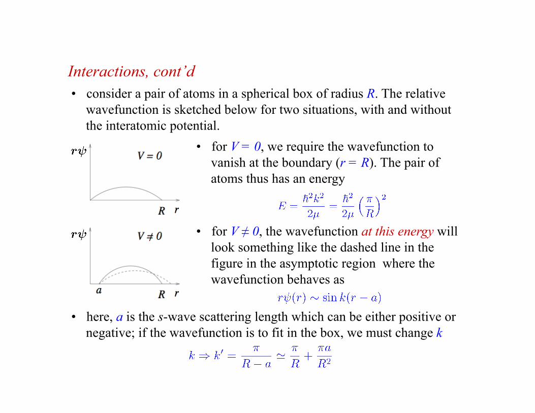
Interactions, cont’d •  consider a pair of atoms in a spherical box of radius R. The relative

wavefunction is sketched below for two situations, with and without the interatomic potential.

•  for V = 0, we require the wavefunction to vanish at the boundary (r = R). The pair of atoms thus has an energy

•  for V ≠ 0, the wavefunction at this energy will look something like the dashed line in the figure in the asymptotic region where the wavefunction behaves as

•  here, a is the s-wave scattering length which can be either positive or negative; if the wavefunction is to fit in the box, we must change k

Interactions, cont’d •  the change in energy of the state is thus

•  if we multiply this by the number of atoms in the gas, we have

•  this is effectively the energy required to place an atom into a gas of density n; when done more carefully, the interaction between atoms can be represented by the pseudopotential

•  if a is positive (negative) the effective interaction is repulsive (attractive); interestingly, this ‘interaction’ is associated with a change in kinetic energy of the gas! This short-ranged potential can be used as the effective interaction but care must be exercised when doing so.

Variational Ground State of the Interacting Gas •  the complete second-quantized Hamiltonian is

•  this state has all the particles in a single quantum state ϕ0(r); we then have

•  let’s expand the field operator in a single-particle basis (e.g. trap states)

and consider the variational ground state

•  this must now be minimized with respect to ϕ0(r); the normalization constraint is achieved by means of a Lagrange parameter and we then minimize freely

The Time-independent Gross-Pitaevskii Equation •  in this way we arrive at the celebrated Gross-Pitaevskii equation

where the condensate wavefunction is

•  because of the interactions, the GP equation is nonlinear and the usual properties of the linear Schrödinger equation no longer apply; this state is the closest one can come in an interacting Bose gas to putting all the particles into the ‘lowest quantum state’

•  the nonlinearity of the GP equation typically requires an iterative procedure in order to obtain its solutions

•  the ‘ground’ state is not the only state of physical interest; ‘excited’ states are also accessible experimentally

•  as we shall see, there is also a dynamical version of this equation

E: Show that the variation of K leads to the GP equation.

The Thomas-Fermi Approximation •  it is not straightforward to solve the nonlinear GP equation; there is

however a remarkably simple and accurate solution when the number of particles is large

•  neglecting the kinetic energy term in the GP equation we obtain

•  this is an explicit expression for the condensate density nc0(r) = |Φ0(r)|2

which is valid when µ0 < Vtrap(r); for a harmonic trap, the density profile is an inverted parabola; the chemical potential µ0 controls the number of particles N in the trap

•  the TF radius is given by

•  the approximation is valid if

•  the approximation breaks down at the edge of the condensate

So, what exactly is the condensate wavefunction? •  at first sight the condensate wavefunction may seem rather mysterious •  the single-particle density matrix provides some insight. Recall

•  in terms of these eigenfunctions – natural orbitals – we have

•  the total number of particles is thus given by

That is, the eigenvalues can be interpreted as the occupation numbers of the natural orbitals; we have isolated the largest eigenvalue n0. For a Bose-condensed system, this eigenvalue will be of order N. We say that the corresponding orbital is macroscopically occupied.

OK, now we’re beginning to see what it means! •  defining we have

•  if we now suppose that (Bogoliubov, 1947)

we have

•  in other words, the assumption of Bose broken symmetry reproduces the form of the single particle density matrix. The expectation value of the field operator plays the role of the order parameter for the Bose superfluid phase transition:

•  note in general that

•  in an interacting system this is true even at T = 0: quantum depletion

Bose Broken Symmetry •  of course in a conventional average involving states with a definite

number of particles we must have

•  so in what sense can this average be nonzero? If we imagine introducing into the Hamiltonian a symmetry breaking perturbation

the Hamiltonian is no longer number-conserving and the field operator can have a finite average. If we then find

we can say that the system is Bose-condensed. This is analogous to what is done for a magnetic phase transition – there we introduce a weak magnetic field which breaks the isotropy of space, thereby allowing the magnetization to point in a given direction. Here the symmetry-breaking perturbation fixes the phase of the order parameter. When all is said and done, we can simply assume in the theory that for a Bose-condensed system.

The Time-dependent GP equation •  if we are not dealing with an equilibrium situation, the order parameter

will be time-dependent. The condensate wavefunction is then described by the time-dependent GP equation

•  this equation seems an obvious generalization of the time-independent GP equation but I will not justify it at this point since a detailed derivation will be provided in Lecture 2. The point is that this equation can describe the dynamics of the condensate at T = 0. In particular, it can be used to study the collective modes of the condensate, or the normal modes of oscillation. I want to illustrate this with a few examples.

•  first, let’s reformulate the TDGP equation using the amplitude-phase representation of the condensate wavefunction:

The Time-dependent GP equation, cont’d •  substituting this into the TDGP equation, the left hand side is

and the right hand side becomes

•  equating real and imaginary parts of these equations, we arrive at

with

E: Derive these equations.

The Time-dependent GP equation, cont’d •  we have thus reduced the TDGP equation to two coupled equations in

the ‘hydrodynamic’ variables nc and vc which are similar to the hydrodynamic equations for a normal fluid.

•  the dynamic TF approximation neglects the ‘quantum pressure’ term in the chemical potential. The equations can be linearized by introducing

•  assuming vc0 = 0, we obtain the Stringari equation (1996)

E: Derive this equation. •  this equation was first derived by Stringari in 1996. It has been very

useful in the study of the collective modes in a pure condensate at T = 0: more about this in Lecture 3.

Sound Waves in a Uniform Condensate •  in a uniform Bose gas (no trapping potential) the normal mode

solutions are plane waves

•  substituting this into the Stringari equation we obtain

with the solution

•  the collective mode is a phonon-like excitation with a sound speed of

•  if the quantum pressure term is retained, the excitation frequency is given by the Bogoliubov result (also see Lecture 3)

E: Obtain this result by retaining and linearizing the quantum pressure term in the hydrodynamic equations.

The Kohn Theorem •  to conclude this first lecture let’s obtain an important result for atoms

confined by a harmonic potential. This result was first established by Kohn (1961) in the context of the cyclotron resonance in metals and extended to harmonically-confined electrons by Dobson (1994).

•  assume the Hamiltonian

and define the centre-of-mass position operator

•  the Heisenberg equation of motion for this operator is

•  from the Heisenberg equation of motion for the momentum operator we find

The Kohn Theorem, cont’d •  this result is independent of the interactions between the particles. In

other words, the centre-of-mass motion separates from the relative motion of the particles. This implies the existence of dipolar oscillations of the centre-of-mass at the frequencies ωα .

•  likewise, one can show that the nonlinear TDGP equation has a solution of the form

where

•  there is thus a solution where the condensate oscillates rigidly about the centre of the trap. A consequence of the Kohn theorem is that such a mode must exist regardless of the state of relative motion of the atoms. In fact, such a mode will exist even at finite temperature.

E: It is instructive to prove this.