The trapped two-dimensional Bose gas: from Bose-Einstein ...

HAL Id: hal-00194992https://hal.archives-ouvertes.fr/hal-00194992v3

Submitted on 25 Feb 2008

HAL is a multi-disciplinary open accessarchive for the deposit and dissemination of sci-entific research documents, whether they are pub-lished or not. The documents may come fromteaching and research institutions in France orabroad, or from public or private research centers.

L’archive ouverte pluridisciplinaire HAL, estdestinée au dépôt et à la diffusion de documentsscientifiques de niveau recherche, publiés ou non,émanant des établissements d’enseignement et derecherche français ou étrangers, des laboratoirespublics ou privés.

The trapped two-dimensional Bose gas: fromBose-Einstein condensation to

Berezinskii-Kosterlitz-Thouless physicsZoran Hadzibabic, Peter Krüger, Marc Cheneau, Steffen Patrick Rath, Jean

Dalibard

To cite this version:Zoran Hadzibabic, Peter Krüger, Marc Cheneau, Steffen Patrick Rath, Jean Dalibard. Thetrapped two-dimensional Bose gas: from Bose-Einstein condensation to Berezinskii-Kosterlitz-Thouless physics. New Journal of Physics, Institute of Physics: Open Access Journals, 2008, 10,pp.045006. �10.1088/1367-2630/10/4/045006�. �hal-00194992v3�

https://hal.archives-ouvertes.fr/hal-00194992v3

https://hal.archives-ouvertes.fr

hal-

0019

4992

, ver

sion

3 -

25

Feb

2008

The trapped two-dimensional Bose gas:

from Bose-Einstein condensation to

Berezinskii-Kosterlitz-Thouless physics

Z. Hadzibabic1,2, P. Kruger1,3,4, M. Cheneau1, S. P. Rath1 and

J. Dalibard1

1 Laboratoire Kastler Brossel, CNRS, Ecole normale superieure, 24 rue Lhomond,

75005 Paris, France2 Cavendish Laboratory, University of Cambridge, Cambridge CB3 0HE, United

Kingdom3 Kirchhoff Institut fur Physik, Universitat Heidelberg, 69120 Heidelberg, Germany4 Midlands Centre for Ultracold Atoms, School of Physics and Astronomy, University

of Nottingham, Nottingham NG7 2RD, United Kingdom.

E-mail: [email protected]

Abstract. We analyze the results of a recent experiment with bosonic rubidium

atoms harmonically confined in a quasi-two-dimensional geometry. In this experiment

a well defined critical point was identified, which separates the high-temperature

normal state characterized by a single component density distribution, and the low-

temperature state characterized by a bimodal density distribution and the emergence

of high-contrast interference between independent two-dimensional clouds. We first

show that this transition cannot be explained in terms of conventional Bose-Einstein

condensation of the trapped ideal Bose gas. Using the local density approximation,

we then combine the mean-field (MF) Hartree-Fock theory with the prediction for

the Berezinskii-Kosterlitz-Thouless transition in an infinite uniform system. If the

gas is treated as a strictly 2D system, the MF predictions for the spatial density

profiles significantly deviate from those of a recent Quantum Monte-Carlo (QMC)

analysis. However when the residual thermal excitation of the strongly confined degree

of freedom is taken into account, an excellent agreement is reached between the MF and

the QMC approaches. For the interaction strength corresponding to the experiment,

we predict a strong correction to the critical atom number with respect to the ideal

gas theory (factor ∼ 2). A quantitative agreement between theory and experiment is

reached concerning the critical atom number if the predicted density profiles are used

for temperature calibration.

The trapped two-dimensional Bose gas 2

1. Introduction

As first noticed by Peierls [1], collective physical phenomena in an environment with

a reduced number of dimensions can be dramatically changed with respect to our

experience in three dimensions. The example of Bose-Einstein condensation in a uniform

gas is a good illustration of the crucial role of dimensionality. In three dimensions (3D),

condensation occurs at a finite temperature, and the phase of the macroscopic wave

function exhibits long range order [2]. In two dimensions, such long range order is

destroyed by thermal fluctuations at any finite temperature, both for an ideal and for

an interacting Bose gas [3, 4].

In presence of repulsive interactions between particles, a uniform 2D Bose gas can

nevertheless undergo a phase transition from a normal to a superfluid state at a finite

critical temperature. This transition was predicted by Berezinskii [5] and by Kosterlitz

and Thouless [6] (BKT), and it has been observed in several macroscopic quantum

systems, such as helium films adsorbed on a substrate [7]. The superfluid state exhibits

quasi-long range order, such that the one-body correlation function decays algebraically

at large distance. By contrast the decay is exponential in the normal phase.

The recent advances in the manipulation of quantum atomic gases have made it possible

to address the properties of low-dimensional Bose gases with novel tools and diagnostic

techniques [8, 9, 10, 11, 12, 13, 14, 15, 16, 17, 18] (for recent reviews, see [19, 20]).

A recent cold atom experiment also addressed the BKT problem by realizing a two-

dimensional array of atomic Josephson junctions [21]. All these systems bring new

questions, since one is now dealing with a harmonically trapped, instead of a uniform,

fluid. In particular, due to a different density of states, even in 2D one expects to

recover the Bose-Einstein condensation phenomenon in the ideal Bose gas case [22].

The total number of atoms in the excited states of the trap is bounded from above,

and a macroscopic population of the ground state appears for large enough atom

numbers. However real atomic gases do interact. It is therefore a challenging question to

understand whether in presence of atomic interactions, a trapped Bose gas will undergo

a BKT superfluid transition like in the uniform case, or whether conventional Bose-

Einstein condensation will take place, as for an ideal system.

In recent experiments performed in our laboratory [17, 18], a gas of rubidium atoms

was trapped using a combination of a magnetic trap providing harmonic confinement

in the xy plane, and an optical lattice, ensuring that the third degree of freedom (z) of

the gas was frozen. The analysis of the atomic density profile revealed a critical point,

between a high temperature phase with a single component density distribution, and a

low temperature phase with a clear bimodal distribution [18]. This critical point also

corresponded to the onset of clearly visible interferences between independent gases,

which were used to study the coherence properties of the system [17]. Surprisingly,

the density profile of the normal component was observed to be close to a gaussian all

the way down (in temperature) to the critical point. This density profile is strikingly

different from the one expected for the ideal gas close to the BEC critical temperature.


Furthermore, if the width of the observed quasi-gaussian distribution is interpreted as

an empirical measure of the temperature, this leads to a critical atom number at a given

temperature which is about five times larger than that needed for conventional Bose-

Einstein condensation in the ideal gas. These two facts showed that, in sharp contrast

to the 3D case, interactions in 2D cannot be treated as a minor correction to the ideal

gas BEC picture, but rather qualitatively change the behavior of the system.

The main goal of the present paper is to analyze this critical point. We start in § 2 with

a brief review of the properties of an ideal Bose gas in the uniform case and in the case

of harmonic confinement. In § 3 we adapt the ideal gas treatment to the experimental

geometry of [18], and provide a detailed calculation showing that the experimental

results cannot be explained by this theory. Next, in § 4, we take interactions into

account at the mean-field (MF) level and we combine this analysis with the numerically

known threshold for the BKT transition in the uniform case [23]. We first present a

MF treatment for a strictly 2D gas. For the parameter range explored experimentally,

it leads to a critical atom number in good agreement with the prediction of the most

recent Quantum Monte Carlo (QMC) calculations [24]. However the predicted MF

density profiles significantly differ from the QMC ones in the vicinity of the critical point.

In a second step, we take into account the residual excitation of the z motion in the

mean-field model and we obtain an excellent agreement with the QMC calculation. The

predicted density distribution near the critical point has a quasi-gaussian shape and the

“empirical” temperature extracted from this distribution is in fact somewhat lower than

the real temperature. Taking this into account we obtain good quantitative agreement

between experimental results and theoretical predictions. Finally we summarize our

findings and discuss the connection between the BEC and the BKT transition in a 2D

gas. While in a uniform, infinite system only the latter can occur at finite temperature,

in a trapped gas both are possible, and the BEC transition can be viewed as a special,

non-interacting limit of the more general BKT behavior.

2. Bose-Einstein condensation in an ideal 2D Bose gas

This section is devoted to a review of well known results concerning the ideal Bose gas

in two dimensions. We first address the case of a uniform system at the thermodynamic

limit, and we then consider a gas confined in a harmonic potential.

2.1. The uniform case

In the thermodynamic limit a uniform, ideal Bose gas does not undergo Bose-Einstein

condensation when the temperature T is reduced, or the 2D spatial density n is

increased. Bose-Einstein statistics leads to the following relation between the phase

space density D = nλ2 and the fugacity Z = exp(βµ)

D = g1(Z) , gα(Z) =∞∑

j=1

Zj/jα . (1)


Here λ = h(2π/(mkBT ))1/2 is the thermal wavelength, m is the atomic mass, β =

1/(kBT ) and µ is the chemical potential. The function gα(Z) is the polylogarithm, that

takes the simple form g1(Z) = − ln(1 − Z) for α = 1. Because g1(Z) → +∞ when

Z → 1, (1) has a solution in Z for any value of D. Hence no singularity appears in the

distribution of the population of the single particle levels, even when the gas is strongly

degenerate (D ≫ 1). This is to be contrasted with the well known 3D case: the relation

D(3D) = g3/2(Z) ceases to have a solution for a phase space density above the critical

value D(3D)c = g3/2(1) ≃ 2.612, where the 3D Bose-Einstein condensation phenomenon

takes place.

2.2. The ideal 2D Bose gas in a harmonic confinement

We now consider an ideal gas confined in a harmonic potential V (r) = mω2r2/2. We

assume that thermal equilibrium has been reached, so that the population of each energy

level is given by Bose-Einstein statistics. Since the chemical potential µ is always lower

than the energy hω of the ground state of the trap, the number of atoms N ′ occupying

the excited states of the trap cannot exceed the critical value N (id)c

N (id)c =

+∞∑

j=1

j + 1

exp(jβhω) − 1. (2)

This expression can be evaluated in the so-called semi-classical limit kBT ≫ hω by

replacing the discrete sum by an integral over the energy ranging from 0 to +∞ [22]:

N (id)c =

(

kBT

hω

)2

g2(1) , (3)

with g2(1) = π2/6. This result also holds in the case of an anisotropic harmonic potential

in the xy plane, in which case ω is replaced by the geometric mean ω =√

ωxωy, where

ωx, ωy are the two eigenfrequencies of the trap. The saturation of the number of atoms

in the excited states is a direct manifestation of Bose-Einstein condensation: any total

atom number N above N (id)c must lead to the accumulation of at least N −N (id)

c in the

ground state of the trap.

Equation (3) is very reminiscent of the result for the harmonically trapped 3D gas,

where the saturation number is N (3D,id)c = (kBT/(hω))3 g3(1). However an important

difference arises between the 2D and the 3D cases for the spatial density profile. In 3D

the phase space density in r is given by D(3D)(r) = g3/2(Ze−βV (r)) in the limit kBT ≫ hω.

The threshold for Bose-Einstein condensation is reached for Z = 1; at this point N is

equal to the critical number N (3D,id)c and simultaneously the phase space density at the

center of the trap D(3D)(0) equals the critical value g3/2(1). This allows for a simple

connection between the BEC thresholds for a homogenous gas and for a trapped system

in the semi-classical limit kBT ≫ hω. In 2D such a simple connection between global

properties (critical atom number N (id)c ) and local properties (critical density at center

n(0)) does not exist. Indeed the semi-classical expression of the 2D phase space density

is

D(r) = g1(Ze−βV (r)) . (4)


Because g1(1) = +∞ this leads to a diverging value at the center of the trap when Z

approaches 1. Therefore, although the integral of D(r) over the whole space converges

for Z = 1 and allows to recover (3), the semiclassical result (4) cannot be used to derive

a local criterion for condensation at the center of the trap.

One can go beyond the semi-classical approximation and calculate numerically the

central phase space density as a function of the total number of atoms. We consider as an

example the trap parameters used in [18], where ωx/(2π) = 9.4 Hz, ωy/(2π) = 125 Hz.

In the typical case kBT/(hω) = 50 (T ≃ 80 nK), the discrete summation of the Bose-

Einstein occupation factors for Z = 1 gives Nc ≃ 4800 (the value obtained from the

semi-classical result (3) is 4100). Using the expression of the energy eigenstates (Hermite

functions), we also calculate the phase space density at the origin and we find D(0) ≃ 13.

Let us emphasize that this value is a mere result of the finite size of the system, and

does not have any character of universality.

3. Condensation of an ideal Bose gas in a harmonic + periodic potential

In order to produce a quasi two-dimensional gas experimentally, one needs to freeze the

motion along one direction of space, say z. In practice this is conveniently done using

the potential V (lat)(z) = V0 sin2(kz) created by an optical lattice along this direction.

A precise comparison between the measured critical atom number and the prediction

for an ideal gas requires to properly model the confining potential and find its energy

levels. This is the purpose of the present section.

3.1. The confining potential

The optical lattice is formed by two running laser waves of wavelength λL, propagating

in the yz plane with an angle ±θ/2 with respect to the y axis. The period ℓ = π/k =

λL/(2 sin(θ/2)) of the lattice along the z direction can be adjusted to any value above

λL/2 by a proper choice of the angle θ. For a blue-detuned lattice (λL is smaller than the

atomic resonance wavelength), V0 is positive and the atoms accumulate in the vicinity

of the nodal planes z = 0, z = ±π/k, etc. The oscillation frequency at the bottom of

the lattice wells is ω(lat)z = 2

√V0Er/h, where Er = h2k2/(2m). In order for the quasi-2D

regime to be reached, hω(lat)z must notably exceed the typical thermal energy kBT as

well as the interaction energy per particle for a non ideal gas.

For a blue detuned lattice an additional confinement in the xy plane must be added to

the optical lattice potential. This is conveniently achieved using a magnetic trap, that

creates a harmonic potential with frequencies ωx, ωy. The magnetic trap also provides an

additional trapping potential mω2zz

2/2 along the z direction. The oscillation frequency

ωz created by the magnetic trap is usually much lower than the one created by the

lattice ω(lat)z . The main effect of the magnetic confinement along the z direction is to

localize the atoms in the N central lattice planes, where the effective number of planes

N ∼ 4 kBT/(mω2zℓ

2). As we see below this number is on the order of 2 to 4 for the range


of parameters explored in [18]. The fact that more than just one plane is populated is

an important ingredient of the experimental procedure used in [17, 18]. It allows one to

look for the interferences between planes, and to access in this way the spatial coherence

of the quasi-2D gas.

In order to extract thermodynamic information from the interference between planes,

one must ensure that the various populated planes have the same temperature. This is

achieved by using finite size lattice beams in the xy plane, so that atoms in the high

energy tail of the thermal distribution can actually travel quasi freely from one plane

to the other, thus ensuring thermalization. In the experiments described in [17, 18], the

waist Wx of the lattice beams along the x direction was chosen accordingly. The total

trapping potential can then be written in the following way

V (r) = V (mag)(r) + V (lat)(r) (5)

with

V (mag)(r) =1

2m(

ω2xx

2 + ω2yy

2 + ω2zz

2)

(6)

V (lat)(r) = V0 e−2x2/W 2x sin2(k(z − z0)) (7)

Note that we have included here the offset z0 between the optical lattice and the bottom

of the magnetic potential; this quantity was not set to a fixed value in the experiments

[17, 18]. We consider below two limiting situations: (A) kz0 = π/2, with two principal

equivalent minima in kz = ±π/2, (B) kz0 = 0, with one principal minimum in z = 0

and two side minima in kz = ±π. At very low temperatures, we expect that A will

lead to two equally populated planes whereas configuration B will lead to one populated

plane. For the temperature range considered in practice, the differences between the

predictions for A and B are minor, as we will see below.

3.2. Renormalization of the trapping frequency ωx by the optical lattice

In order to use the Bose-Einstein statistics for an ideal gas, one needs to know the

position of the single particle energy levels. For the potential (5) it is not possible to

find an exact analytical expression of these levels. However if the extension of the atomic

motion along the x direction is smaller than the laser waist, an approximate expression

can be readily obtained, as we show now.

The frequencies of the magnetic trap used in [17, 18] are ωx = 2π × 10.6 Hz and

ωy = ωz = 2π × 125 Hz. The optical lattice has a period π/k = 3 µm (Er =

h2k2/(2m) = h × 80 Hz) and a potential height at center U0/h = 35 kHz (1.7 µK).

The lattice oscillation frequency at center (x = 0) is thus ω(lat)z (x = 0) = 2π × 3 kHz

(hω(lat)z /kB = 150 nK). When the atoms occupy the ground state of the z motion,

they acquire the zero-point energy hω(lat)z (x)/2 from the z−degree of freedom. The

dependance on x of ω(lat)z (x), due to the gaussian term e−2x2/W 2

x in the laser intensity,

causes a renormalization of the x frequency:

ω2x → ω′2

x = ω2x −

2√

V0Er

mW 2x

. (8)


The waist of the lattice beams is Wx = 120 µm which leads to ω′

x = 2π × 9.4 Hz. A

similar effect should in principle be taken into account for the frequency ωy. However

the scale of variation of the laser intensity along the y axis is the Rayleigh length, which

is much larger than the waist Wx, and the effect is negligible.

This simple way of accounting for the finiteness of the waist Wx is valid when the

extension of the motion along x is small compared to Wx. For T = 100 nK, the width of

the thermal distribution along x is√

kBT/mω2x ∼ 50 µm, which is indeed notably smaller

than Wx. Taking into account the finiteness of Wx by a mere reduction of the trapping

frequency along x is therefore valid for the major part of the energy distribution.

We note however that atoms in the high energy tail of the distribution (E > 5 kBT for

our largest temperatures) can explore the region |x| > Wx, where the influence of the

lattice beams is strongly reduced. In this region the atoms can move from one lattice

plane to the other. As explained above these atoms play an important role by ensuring

full thermalization between the various planes. We now turn to an accurate treatment of

the critical atom number required for Bose-Einstein condensation, taking into account

these high energy levels for which the 2D approximation is not valid.

3.3. The critical atom number in a ‘Born–Oppenheimer’ type approximation

In order to get the single particle energy eigenstates in the lattice + harmonic potential

confinement, and thus the critical atom number, one could perform a numerical

diagonalization of the 3D hamiltonian with the potential (5). This is however a

computationally involved task and it is preferable to take advantage of the well separated

energy scales in the problem.

We first note that the trapping potential (5) is the sum of a term involving the variables

x and z, and a quadratic component in y. The motion along the y axis can then

be separated from the xz problem, and it is easily taken into account thanks to its

harmonic character. For treating the xz problem we use a ‘Born-Oppenheimer’ type

approximation. We exploit the fact that the characteristic frequencies of the z motion

are in any point x notably larger than the frequency of the x motion. This is of course

true inside the lattice laser waist, since ω(lat)z /ωx ∼ 300, and it is also true outside

the laser waist as the x direction corresponds to the weak axis of our magnetic trap.

Therefore we can proceed in two steps:

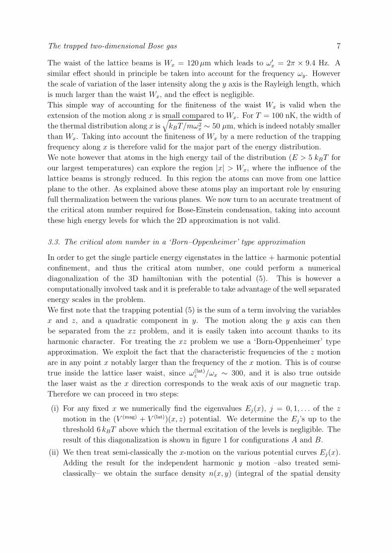
(i) For any fixed x we numerically find the eigenvalues Ej(x), j = 0, 1, . . . of the z

motion in the (V (mag) + V (lat))(x, z) potential. We determine the Ej’s up to the

threshold 6 kBT above which the thermal excitation of the levels is negligible. The

result of this diagonalization is shown in figure 1 for configurations A and B.

(ii) We then treat semi-classically the x-motion on the various potential curves Ej(x).

Adding the result for the independent harmonic y motion –also treated semi-

classically– we obtain the surface density n(x, y) (integral of the spatial density


0 50 100 150 0

5000

10000

15000 E

nerg

ies

E j (

Hz)

x (micrometers)

0 50 100 150 0

5000

10000

15000

Ene

rgie

s E

j (H

z)

x (micrometers)

Figure 1. Eigenvalues of the z-motion in the magnetic+optical x − z potential, for

fixed values of the x coordinate (left: configuration A, right: configuration B).

n3(r) along the direction z)

n(x, y) =1

λ2

∑

j

g1

(

Ze−β(Ej(x)+V (mag)(y)))

. (9)

This procedure yields a result that is identical to the semi-classical prediction in two

limiting cases:

(i) The pure 2D case, that is recovered for large waists and low temperatures. In this

case the restriction to the closest-to-center lattice plane and to the first z-level is

legitimate, and the sum over j contains only one significant term corresponding to

(4).

(ii) the pure 3D harmonic case with zero lattice intensity where Ej(x) = mω2xx

2/2 +

(j + 1/2)hωz. In this case the sum over j in (9) leads to n(x, y) λ2 =

g2

(

Ze−βV (mag)(x,y))

/(βhωz), which coincides with the 3D result D(3D)(r) =

g3/2(Ze−βV (r)) when integrated along z.

Of course this procedure also allows to interpolate between these two limiting

cases, which is the desired outcome. The integral of n in the xy plane for µ =

min(

Ej(x) + V (mag)(y))

gives the critical atom number N (lat,id)c (T ) in the ideal gas

model for this lattice geometry. It is shown in figure 2a for the two configurations

A and B.

The critical atom number N (lat,id)c can be compared with the result for a single plane

N (id)c with eigenfrequencies ω′

x and ωy. The ratio gives the effective number of planes

Neff , shown as a function of temperature in figure 2b for the two configurations A and B.

This ratio increases with temperature, which means that N (lat,id)c increases faster than

T 2 with temperature in the temperature domain considered here. For example in the

range 50 − 110 nK, the variation of N (lat,id)c is well represented by T β, with β = 2.8.

Three phenomena contribute significantly to this “faster than T 2” increase of N (lat,id)c .

First in the lattice + harmonic potential geometry, the number of contributing planes

increases with temperature, even if the atomic motion in each plane remains two-


dimensional (i.e. the atom number per plane increasing strictly as T 2). Second, we

are exploring here a region of temperature where kBT becomes non negligible with

respect to hω(lat)z (the two quantities are equal for T = 150 nK), and the thermal

excitations of the z-motion in each lattice plane cannot be fully neglected. Third, for

the largest considered temperatures, the extension of the atomic motion along x becomes

comparable to the laser waist, and the lattice strength is then significantly reduced.

0 25 50 75 100 125 150 175 0

40000

80000

120000

160000 (a)

criti

cal a

tom

num

ber

temperature (nK) 0 25 50 75 100 125 150 175

1

2

3

4

5

6

7

8 (b)

Effe

ctiv

e nu

mbe

r of

pla

nes

temperature (nK)

Figure 2. (a) Critical atom number N(lat,id)c in the ideal gas model for the optical

lattice + magnetic trap configuration, as a function of temperature. The points

represent the experimental results of [18], and the error bars combine the systematic

and statistical uncertainties on atom numbers. (b) Effective number of planes

Neff = N(lat,id)c /N

(id)c as a function of temperature. In both panels the continuous

(dashed) line is for configuration A (B). The calculation is performed using the first

100 eigenvalues of the z motion, and the first neglected levels Ej(x) are 22 kHz (1 µK)

above the bottom of the trap.

3.4. Comparison with experimental results

In [18] the critical atom number in the lattice + magnetic trap configuration was

measured for various “effective” temperatures, deduced from the width of the quasi-

gaussian atomic distribution. Each critical point (N (exp)c , T (exp)

c ) was defined as the

place where a bimodal spatial distribution appeared, if the atom number was increased

beyond this point at constant temperature, or the temperature reduced at constant

atom number. The critical point also corresponded to the threshold for the appearance

of interferences with a significant contrast between adjacent planes. The experimental

measurements of critical points, taken over the effective temperature range 50–110 nK,

are shown as dots in figure 2a. The systematic + statistical uncertainties of the atom

number calibration are 25%. Assuming that the effective temperatures coincide with

the true ones (this point will be examined in § 4.6) we find N (exp)c /N (lat,id)

c ∼ 5.3 (±1.2).

In addition to this large discrepancy between experiment and ideal gas model for the

critical atom numbers, one also finds a strong mismatch concerning the functional shape

of the column density∫

n(x, y)dy that was measured in absorption imaging in [17, 18].


While the experimental result is quasi-gaussian, the column density profiles calculated

for an ideal gas at the critical point are much ‘peakier’. An example is given in the

appendix for a single plane, and we checked that a similar shape remains valid for our

harmonic + lattice potential. We therefore conclude that the experimental results of

[18] cannot be accounted for with this ideal gas prediction for ‘conventional’ BEC.

4. Interactions in a quasi 2D trapped Bose gas

To improve the agreement between the experimental results and the theoretical modeling

we now take repulsive atomic interactions into account. In a first stage we present a

2D mean-field analysis, in which the motion along z is assumed to be completely frozen

whereas the xy motion is treated semi-classically. In order to model interactions in

this case, we start from the 3D interaction energy (g(3D)/2)∫

n23(r) d3r, where g(3D) =

4πh2a/m and a is the scattering length. The z-degree of freedom is restricted to the

gaussian ground state of the confining potential, with an extension az =√

h/(mω(lat)z ),

and the interaction energy is

Eint =g

2

∫

n2(r) d2r .

We set g = h2g/m, where the dimensionless parameter g =√

8π a/az characterizes the

strength of the 2D interaction (for a more elaborate treatment of atomic interactions in a

quasi-2D geometry, see [25, 26]). For the optical lattice used in [18] we find g = 0.13. In

a second stage we take into account the residual excitation of the z-motion in a ‘hybrid’

3D mean-field approximation. We calculate in a self-consistent way the quantum levels

of the z motion, whereas the motion in the xy plane is still treated semi-classically.

4.1. Criticality within mean-field solutions: 3D vs. 2D

We start our discussion with a brief reminder of the role of (weak) interactions in a

trapped 3D Bose gas [27]. One often uses the mean-field Hartree-Fock approximation,

that gives in particular a relatively accurate value for the shift of the critical temperature

for Bose-Einstein condensation. In order to calculate this shift, one assumes that

above the critical temperature, the atoms evolve in the effective potential Veff(r) =

V (r) + 2g(3D)n3(r). The phase space density in r is thus a solution of D(3D)(r) =

g3/2(Ze−βVeff (r)). As for the ideal case this equation ceases to have a solution when the

central phase space density goes above g3/2(1). The mere effect of repulsive interactions

within the mean-field approximation is to increase the number of atoms for which this

threshold is met. The increase is typically ∼ 10% for standard trap and interaction

parameters [27].

For a trapped 2D gas this treatment based on a local criterion (phase space density at

center) cannot be used. Indeed as explained in section 2.2, it is not possible to identify

a critical phase space density at which BEC of the 2D gas is expected. On the contrary

the semiclassical approximation leads to an infinite central density at the critical point,


and it is unclear whether one can achieve an arbitrarily large spatial density in presence

of repulsive interactions.

One could also look for a global criterion for criticality based on the total atom number.

The starting point is the solution of the mean-field equation

D(r) = g1

(

Ze−βVeff (r))

(10)

with Veff(r) = V (r) + 2g n(r). When g = 0, we saw in §2 that the solution of (10) can

only accommodate a finite number of atoms (3). However the situation is dramatically

changed in presence of repulsive interactions. Indeed for any non zero g, a solution to

(10) exists for arbitrarily large atom numbers [28]. Consequently no critical point can

be found by simply searching for a maximal atom number compatible with (10). In

the following we will therefore turn to a different approach, starting from the known

exact (i.e. non mean-field) results concerning the critical BKT point in a uniform

interacting 2D Bose gas. The mean-field approximation will be used in a second stage,

in combination with the local density approximation (LDA), to determine the critical

atom number in the trapped system.

Note that it is also possible to pursue the search for a critical point only within the mean-

field approach, by looking for example whether its solution exhibits a thermodynamical

or dynamical instability above a critical atom number [29, 30]. This instability would

be an indication that the system tends to evolve towards a different kind of state, with

a non-zero quasi-condensed and/or superfluid component, and quasi-long range order

[31, 32].

4.2. The Berezinskii-Kosterlitz-Thouless transition and the local density approximation

In an infinite uniform 2D Bose fluid, repulsive interactions have a dramatic effect

since they can induce a transition from the normal to the superfluid state, when the

temperature is lowered below a critical value. The superfluid density jumps from 0

to 4/λ2 at the transition point [33]. The microscopic mechanism of the 2D superfluid

transition has been elucidated by Berezinskii [5] and by Kosterlitz and Thouless [6].

For a temperature larger than the critical temperature, free vortices proliferate in the

gas, destroying the superfluidity. Below the transition, vortices exist only in the form of

bound pairs involving two vortices of opposite circulations, which have little influence

on the superfluid properties of the system.

In a uniform system the phase space density D is a function of the chemical potential

and temperature D = F (µ, T ). For any given T , the superfluid transition occurs when

µ is equal to a critical value µc(T ). The corresponding critical value Dc for the phase

space density depends on the interaction strength as [34, 35, 36]

Dc = ln(ξ/g) (11)

where ξ is a dimensionless number. A recent Monte-Carlo analysis provided the result

ξ = 380 ± 3 [23] (see also [37]). For g = 0.13 this gives a critical phase space density

Dc = 8.0.


(a)

x c

y

x

200000 250000 300000 350000 0

10

20

30 (b)

n col ( x

c )

(ar

bitr

ary

units

)

Total atom number

Figure 3. Check of the local density approximation (LDA). (a) The column density

ncol is measured at the edge x = xc of the central part (in grey) of the bimodal

distribution. (b) ncol(xc) is plotted as a function of the total atom number N in the

harmonic trap + lattice configuration. Within the LDA for a single plane, ncol(xc)

should be independent of N , which is indeed nearly the case. The small variation of

ncol(xc) for large N may be due to the appearance of a non negligible population in

side planes of the optical lattice potential. The data have been taken for the effective

temperature T = 105 nK. Each point is extracted from a single image.

We consider now a trapped gas whose size is large enough to be well described by

the local density approximation (LDA). The phase space density in r is given by

D(r) = F (µ−V (r), T ) and a superfluid component forms around the center of the trap

if the central phase density D(0) is larger than Dc [38]. The edge of the superfluid region

corresponds to the critical line where µ−V (r) = µc. The phase space density along this

line is equal to Dc, independently of the total number of atoms in the trap. This can be

checked experimentally and constitutes a validation of the LDA. The integration of the

experimental data along the line of sight y does not lead to any complication because

the trapping potential is separable, V (r) = V1(x) + V2(y). Therefore the edges of the

superfluid region along the x axis are located in ±xc such that V1(xc) = µ − µc (see

figure 3a), and the column density along the line of sight passing in x = xc is

ncol(xc) =1

λ2

∫

D(xc, y) dy =1

λ2

∫

F (µc − V2(y), T ) dy (12)

which is also independent of the total atom number N . This is confirmed experimentally,

as shown in figure 3b where we plot ncol(xc) as a function of N . The slight increase

(10%) of ncol(xc) for atom numbers larger than 3× 105 may be due to the fact that the

population of additional planes becomes non-negligible for such large N .

The possibility to use the LDA to study the Berezinskii-Kosterlitz-Thouless critical point

in a harmonically trapped quasi-2D Bose gas has been checked recently by Holzmann

and Krauth using a quantum Monte-Carlo analysis [24]. For trap parameters close to the

ones of [18] they have shown that a superfluid component, characterized by a reduced

moment of inertia, indeed appears at the center of the trap when the local phase space

density reaches a critical value close to the prediction (11).


4.3. Density profile in the 2D mean-field theory

In this section we use the mean-field Hartree-Fock approximation (10) to calculate the

density profile of the trapped atomic cloud. As we mentioned above, this equation

admits a solution for any value of the fugacity Z, and therefore for an arbitrarily large

number of particles. Rewriting (10) as

D(r) = − ln(

1 − Ze−gD(r)/πe−βV (r))

(13)

we see that the value of D for any temperature and at any point in space depends only

on the parameter R defined by R2 = (x/xT )2 + (y/yT )2, where xT = (ω2xmβ)−1/2 and

yT = (ω2ymβ)−1/2. The total atom number is given by

N =

(

kBT

hω

)2∫

∞

0D(R) R dR (14)

where D(R) is the solution of the reduced equation

D(R) = − ln(

1 − Ze−gD(R)/πe−R2/2)

. (15)

Quite remarkably this result for D(R) neither depends on the trap parameters, nor on

the temperature. The only relevant parameters are the fugacity Z and the reduced

interaction strength g. The scaling of the atom number N with the temperature and

the trap frequency in (14) is therefore very simple. In particular it does not depend on

the trap anisotropy ωy/ωx but only on the geometric mean ω.

For atom numbers much larger than N (id)c it is interesting to note that the radial

density profile deduced from the mean-field equation (13) exhibits a clear bi-modal

shape, with wings given by n(r)λ2 ≃ Ze−βV (r) and a central core with a Thomas-Fermi

profile 2g n(r) ≃ µ − V (r). However this prediction of a bi-modal distribution using

the Hartree-Fock approximation cannot be quantitatively correct. Indeed the Hartree-

Fock treatment assumes a mean-field energy 2gn. The factor 2 in front of this energy

originates from the hypothesis that density fluctuations are those of a gaussian field

〈n2〉 = 2 〈n〉2. Actually when the phase space density becomes significantly larger than

1, density fluctuations are reduced and one approaches a situation closer to a quasi-

condensate in which 〈n2〉 ∼ 〈n〉2 [23]. Taking into account this reduction could be

done for example using the equation of state obtained from a classical field Monte-Carlo

analysis in [39] .

4.4. Critical atom number in the 2D mean-field approach

We now use the solution of the mean-field equation (13) to evaluate the critical atom

number N (mf)c that is needed to reach the threshold (11) for the BKT transition at the

center of the trap D(0) = ln(ξ/g). For a given interaction strength g we vary the fugacity

Z and solve numerically (13) at any point in space. Examples of spatial density profiles

at the critical point are given in the appendix, both before and after time-of-flight. The

integration of the density profile over the whole xy plane gives the total atom number


0 1 2 3 4 5 6 0

2

4

6

8

10

12

14 (a)

1

0.3

0.1

0.03 0.01

Cen

tral

pha

se s

pace

den

sity

N / N c

(id) 0 1 2 3 0.0

0.2

0.4

0.6

0 2 4 0.1

1

10

Pha

se s

pace

den

sity

(r / r T ) 2

(b)

norm

aliz

ed c

olum

n de

nsity

x / x T

Figure 4. (a) Central phase space density predicted by the 2D mean field theory,

as a function of the atom number for various interaction strengths g. The dotted line

represents the semi-classical prediction for the ideal gas. The dashed line indicates

where the threshold for superfluidity (11) is met at the center of the trap. (b) Column

density for N = N(mf)c = 36 000 atoms in an isotropic trap (ωx = ωy = ω, g = 0.13,

kBT = 110 ω). The dashed line is the result of the 2D mean-field analysis of § 4.3. The

continuous line is the 3D quantum Monte-Carlo result obtained in [24], with ωz = 83ω

and a = gaz/√

8π. The dots are the result of the hybrid 3D mean-field calculation of

§ 4.5 for the same parameters. Inset: Prediction of the hybrid 3D mean-field approach

for the phase space density (log scale) as a function of r2 (a gaussian distribution leads

to a straight line). Continuous line: total phase space density; dashed line: phase

space density associated to the ground state ϕ1 of the z motion; dash-dot line: phase

space density associated to all other states ϕj , j ≥ 2.

N . From (14) and (15), it is clear that the scaling of N (mf)c with the frequencies ωx,y

and with the temperature is identical to the one expected for an ideal trapped gas.

We have plotted in figure 4a the variation of D(0) as a function of N/N (id)c for various

interaction strengths. For a given atom number the phase space density at center

decreases when the strength of the interactions increases, as expected. The numerical

result for N (mf)c is plotted as a dashed line in figure 4a. We find that it is in excellent

agreement – to better than 1%– with the result of [38]

N (mf)c

N(id)c

= 1 +3g

π3D2

c (16)

over the whole range g = 0 – 1. This analytical result was initially derived in [38]

for g ≪ 1 using an expansion around the solution for the ideal Bose gas, but this

approximation can actually be extended to an arbitrary value of g [40]. The strongly

interacting limit (3gD2c/π

3 > 1) can be easily understood by noticing that in this case,

the atomic distribution (10) nearly coincides with the Thomas-Fermi profile 2gn(r) =

µ − V (r). Using the relation between the total atom number and the central density

for this Thomas-Fermi distribution N = 2πg (n(0)a2ho)

2(with aho = (h/(mω))1/2), one

then recovers the second term of the right-hand side of (16).

Let us emphasize that figure 4a is a mix of two approaches: (i) The mean-field model,


that does not lead in itself to a singularity along the dashed line of figure 4a. (ii) The

BKT theory for a uniform system, which is a beyond mean-field treatment and which

has been adapted to the trapped case using the local density approximation in order to

obtain the critical number indicated by the dashed line.

We now compare the 2D MF prediction with the results of the QMC calculation of

[24], looking first at the critical atom number and then at the density profiles. For

g = 0.13 the mean field prediction for the critical number (16) is N (mf)c /N (id)

c = 1.8.

This is in relatively good agreement with the QMC calculation of [24], which gives

T (QMC)c = 0.70 T (id)

c or equivalently N (QMC)c /N (id)

c = 2.0. The QMC calculation has

been performed for various atom numbers N , for a 3D harmonic trap such that

ωz/ω = 0.43√

N and a 3D scattering length a = gaz/√

8π, with g = 0.13.

The agreement between the 2D MF and the QMC approaches is not as good for the

density profiles close to the critical point. An example is shown in figure 4b, where we

take kBT = 110 hω (N (id)c = 20 000). We choose N = N (mf)

c = 36 000 and we plot the

column density ncol(x) obtained by integrating the spatial density along the directions

y and z. The mean field result is shown as a dashed line, and it notably differs from

the QMC result, plotted as a continuous line. As we show below this disagreement is

essentially a consequence of the residual excitation of the z motion (kBT/(hωz) = 1.4),

that is neglected in the 2D MF approach, whereas it is implicitly taken into account in

the 3D QMC calculation.

4.5. The hybrid 3D mean-field approach

In this section we extend the 2D mean-field treatment to take into account the residual

excitation of the z motion. As pointed out to us by the authors of [24], this is necessary

for a quantitative analysis of the experiment [18], since the temperature and the chemical

potential at the critical point were not very small compared to hω(lat)z , but rather

comparable to it.

We follow here a method related to the one developed in section 3 to analyze the ideal

gas case. We start from a trial 3D density distribution n3(r). At any point (x, y), we

treat quantum mechanically the z motion and solve the eigenvalue problem for the z

variable[

−h2

2m

d2

dz2+ Veff(r)

]

ϕj(z|x, y) = Ej(x, y) ϕj(z|x, y) , (17)

where Veff(r) = m(ω2xx

2 + ω2yy

2 + ω2zz

2)/2 + 2g(3D)n3(r) and∫ |ϕj(z|x, y)|2 dz = 1.

Treating semi-classically the xy degrees of freedom, we obtain a new spatial density

n′

3(r) = − 1

λ2

∑

j

|ϕj(z|x, y)|2 ln(

1 − eβ(µ−Ej(x,y)))

. (18)

We then iterate this calculation until the spatial density n3(r) reaches a fixed point [41].

With this method, we fulfill two goals: (i) We take into account the residual thermal

excitation of the levels in the z direction. (ii) Even at zero temperature we take into

account the deformation of the z ground state due to interactions.


This ‘hybrid 3D mean-field’ method is different from the standard mean-field treatment

used to describe 3D Bose gases. In the latter case, all three degrees of freedom are treated

semi-classically, which is valid when the particle population is distributed smoothly over

several quantum states. This standard 3D mean-field would not be applicable in our

case, where a significant part of the total population accumulates in the lowest state ϕ1.

An example of a result is shown in figure 4b, where we plot the column density ncol(x)

obtained with this hybrid MF method, taking into account the first 5 eigenstates ϕj . The

agreement between the hybrid 3D mean-field prediction and the ‘exact’ QMC prediction

of [24] is excellent. This shows that the predictions of this hybrid 3D mean-field approach

are reliable as long as the superfluid transition has not been reached at the center of

the trap.

We show in the inset the variations of the phase space density D(r). We plot ln(D) as

a function of r2, so that a gaussian distribution would appear as a straight line. The

dashed line is the phase-space density associated to the ground state of the z-motion

ϕ1, and the dash-dot line corresponds to the excited states ϕj, j ≥ 2. The continuous

line is the total phase-space density. At the center of the trap, as a consequence of

Bose statistics, most of the population (80%) accumulate in the ground state ϕ1. For

r ≥ rT , the repartition of the population among the eigenstates of the z motion follows

the Boltzmann law, and ∼ 50% of the atoms occupy the excited states ϕj, j ≥ 2.

A practical consequence of this increasing influence of excited states of the z-motion

with increasing r is that the total phase space density profile is notably closer to a

gaussian distribution than when only the ground state of the z-motion is retained in the

calculation, as it is the case in the 2D mean-field approach.

Finally we mention that we have also developed a simpler version of this hybrid 3D

mean-field analysis, in which the ϕj levels are not calculated self-consistently, but are

assumed to coincide with the energy eigenstates in the potential mω2zz

2/2 (see also [42]).

For the domain of parameters relevant for the experiment, the two approaches lead to

very similar results.

4.6. Mean-field approach for the lattice configuration and comparison with experiment

In order to compare the predictions of the mean-field approach with the experimental

results, we now turn to the lattice geometry, corresponding to a stack of parallel planes

located in zj = z0 + jℓ, j integer. For simplicity we assume that the laser waist Wx is

large compared to the spatial extent of the atomic cloud, so that we can treat the gas as

a superposition of independent harmonically trapped systems. Each system is located

at the vicinity of a nodal plane of the optical lattice, and is treated as a harmonic trap

with frequencies ω′

x, ωy, ω(lat)z . Note that we include here ‘by hand’ the renormalization

ωx → ω′

x of the x frequency due to the finiteness of the laser waist, that we discussed in

§ 3.2. The magnetic trap adds an extra confinement along the z axis with a frequency

ωz so that the chemical potential for the plane zj is µj = µ − mω2z(z0 + jℓ)2/2. We

assume that the critical point is reached when the phase space density associated to the


0 1 2 3 0.0

0.2

0.4

Nor

mal

ized

col

umn

dens

ity

x / x T

0 50 100 150 0

50000

100000

150000

200000

Ato

m n

umbe

r at

crit

ical

poi

nt

Effective temperature (nanoKelvin)

Figure 5. (a) Hybrid 3D mean-field prediction for the normalized column density for

the lattice configuration A, T = 150 nK and N = 110 000 atoms. For these parameters

the phase space density associated to the lowest eigenvalue of the z motion reaches

the critical value Dc at the center of the most populated planes. The dotted line is a

gaussian fit which gives the effective temperature Teff = 0.64 T = 96 nK. (b) Critical

atom number as a function of the effective temperature obtained from a gaussian fit

of the MF result. The continuous line (resp. dashed) line is for configuration A (resp.

B). The points are the experimental results of [18], already shown in fig. 2.

lowest eigenstate ϕ1 in the most populated plane reaches the critical value (11). Once

the corresponding fugacity is determined, we calculate the spatial distribution in each

plane, sum up the various contributions, and integrate the spatial distribution over the

line of sight y to obtain the column density ncol(x).

A typical result for ncol is given in figure 5a for the temperature T = 150 nK and for

the lattice configuration A. The total atom number is 1.1 × 105. It is well fitted by

a gaussian distribution exp(−x2/2x20) (dotted line), so that we can assign an effective

temperature to this distribution Teff = mω2xx

20/kB. In the example of fig.5a, we find

Teff = 0.64 T (96 nK). For the same T and a lattice in configuration B, the effective

temperature obtained with a gaussian fit is Teff = 0.69 T (103 nK) and the total atom

number is N = 1.0 × 105. We have repeated this procedure for temperatures T in the

range 100-200 nK and consistently found the ratio Teff/T in the range 0.6–0.7, with a

quality of the gaussian fit similar to what is shown in figure 5a.

We have plotted in figure 5b the calculated total number of atoms in the lattice at the

critical point, as a function of the effective temperature deduced from the gaussian fit

to the column density. We have also plotted the experimental points of [18] already

shown in figure 2. We remind the reader that the experimental ‘effective’ temperature

is also deduced from a gaussian fit to the measured column density. One reaches in this

way a good agreement between the experimental results and the hybrid 3D mean-field

prediction. The predicted density profiles with the 3D MF approach therefore provide a

satisfactory means for temperature calibration. They indicate in particular that for the

experiment [18], the effective temperatures are typically 30–40% below the real ones.


To improve on the comparison between theory and experiment, a more controlled setup

will be needed with an accurate independent measurement of temperature, as well as

the possibility of addressing only a single or a fixed number of planes.

5. Summary and concluding remarks

In this paper we have analyzed the critical point of a trapped quasi-2D Bose gas. We

have shown that the experimental results of [18] are not in agreement with the ideal Bose

gas theory. The differences are found first at the qualitative level: the predicted shape

for the ideal gas distribution is ‘peaky’ around its center, which clearly differs from the

quasi-gaussian measured profile. Also the measured critical atom numbers Nc(T ) do not

agree with the predictions for the ideal gas. Using the ‘effective’ temperatures obtained

by treating the gaussian profiles as Boltzmann distributions, the measured Nc(T ) are

larger by a factor ∼ 5 than the predicted ones. We then discussed the predictions of

a hybrid approach based on the local density approximation. It combines the density

profile calculated using a mean-field Hartree-Fock treatment, and the known result for

the critical phase space density for the BKT transition in an infinite, uniform 2D Bose

gas [23]. We compared the predictions of this approach with the results of a recent

Quantum Monte-Carlo calculation [24] and reached the following conclusions: (i) If one

is interested only in the critical atom number, it is sufficient to use a strictly 2D mean-

field approach. It leads to the approximate analytical result (16), in good agreement

with the QMC prediction. For the experimental parameters of [18] the critical atom

number is Nc ∼ 2 N (id)c . (ii) In order to calculate accurately the density profiles for the

experimental temperature range (kBT between 0.5 hωz and hωz), it is important to take

into account the residual excitation of the z degree of freedom (the same conclusion has

been reached in [42]). We have presented a hybrid 3D mean-field approximation which

leads to density distributions in excellent agreement with the QMC predictions close to

the critical point. When generalized to the lattice geometry used in the experiment,

the predicted density profiles are close to a gaussian distribution, and a good agreement

between theory and experiment is reached concerning the critical number Nc(T ) when

the predicted density profile is used for temperature calibration.

We now briefly discuss the nature of the critical point that appears in the trapped 2D

Bose gas and compare it with ‘standard’ Bose-Einstein condensation. For a harmonically

trapped ideal gas, we recall that conventional Bose-Einstein condensation is expected

in the thermodynamic limit N → ∞, ω → 0, Nω2 constant. This is a consequence of

the density of states for a quadratic hamiltonian around the zero energy. The price to

pay for this condensation in a 2D system is a diverging atomic density at the center

of the trap. On the contrary when interactions are taken into account, the mean-field

approximation leads to the potential V (r) + 2gn(r) that is flat at the origin (figure 6a

and [38]). The ‘benefit’ of the harmonic trapping potential is lost and the physics of

the trapped interacting gas is very similar to that of a uniform system. In particular

one expects in the thermodynamic limit the appearance of quasi-long range order only,


0.0 0.5 1.0 1.5 2.0 0.0

0.5

1.0

1.5

2.0 (a)

V ( r

) /

k B T

r / r T

0

1 (b)

0

1

2

T c

(id) T c

Temperature

Con

dens

ed fr

actio

n

Figure 6. (a) Trapping potential V (r) in dashed line and effective mean-field potential

Veff(r) = V (r)+2gn(r) in continuous line, for g = 0.13 and a central phase space density

equal to the critical value (11). (b) Schematic representation of the condensed fraction

in a finite 2D Bose gas for a given interaction strength g (continuous line). Two limits

can be considered: (1) thermodynamic limit N → ∞, ω → 0, Nω2 constant; the

condensed fraction tends to zero for any non zero value of g. (2) ideal gas limit g → 0.

with no true Bose-Einstein condensate [25]. ‡ The transition between the ideal and

the interacting case is explicit in equations (11) and (16), where the limit g → 0 gives

Dc → +∞ and N (mf)c /N (id)

c → 1. In particular (16) can be used to separate a ‘BEC-

dominated’ regime where η = 3gD2c/π

3 ≪ 1 and Nc ≃ N (id)c , and a ‘BKT-dominated’

regime, where the contribution of η is dominant and Nc ≫ N (id)c . In the latter case,

the spatial distribution in the mean-field approximation is a Thomas-Fermi disk with

radius RTF and (16) is equivalent (within a numerical factor) to the BKT threshold (11)

for a uniform gas with density n = N/(πR2TF). The rubidium gas studied in [17, 18] is

at the border of the ‘BKT-dominated’ regime (η ≃ 1), whereas previous experiments

performed on quasi-2D gases of sodium atoms [8] corresponded to η ∼ 0.1, well inside

the ‘BEC-dominated’ regime.

Finally, we must take into account the finite size of the gas in our discussion. It is

known from simulations of 2D spin assemblies that for a finite size system, the average

magnetization increases rapidly around the BKT transition [43]. It is at first sight

surprising that this magnetization can be used as a signature of BKT physics, since

it would not exist in an infinite system where a genuine BKT transition takes place.

However it is relevant for all practical 2D situations: as emphasized in [43] one would

need extremely large systems (‘bigger than the state of Texas’) to avoid a significant

magnetization even just below the transition point. A similar phenomenon occurs for

a finite size Bose gas. A few states acquire a large population around the transition

point, and this allows for the observation of good contrast interferences between two

‡ A similar flattening of the mean-field potential occurs in 3D, but it has no important consequence in

this case since true BEC is possible in an infinite, uniform 3D system.


independent gases. In particular the condensed fraction f0 (largest eigenvalue of the

one-body density matrix) is expected to grow rapidly at the critical point, and this

has been quantitatively confirmed by the QMC calculation of [24]. To illustrate this

point we have schematically plotted in figure 6b the expected variations of f0 with

the parameters of the problem. For given g and N , f0 takes significant values for

T < Tc (continuous line). If the strength of the interactions g is kept constant, the

condensed fraction f0 tends to zero for any finite temperature if the thermodynamic

limit is taken (arrow 1 in figure 6b). Note that the superfluid fraction should tend to a

finite value in this limiting procedure. Now one can also keep N constant and decrease

g to zero (arrow 2 in figure 6b). In this case one expects to recover the ideal gas result

f0 = 1 − (T/T (id)c )2 for any value of N . Therefore we are facing here a situation where

two limits do not commute: limN→∞ limg→0 6= limg→0 limN→∞. Of course this does not

cause any problem in practice since none of these limits is reached. In this sense the

phenomenon observed in our interacting, trapped 2D Bose gas is hybrid: the transition

point is due to BKT physics (the density of states of the ideal 2D harmonic oscillator

does not play a significant role because of the flattening of the potential), but thanks

to the finite size of the system, some diagnoses of the transition such as the appearance

of interferences, take benefit of the emergence of a significant condensed fraction.

Acknowledgments

We are indebted to Markus Holzmann and Werner Krauth for numerous discussions, for

providing the Quantum Monte-Carlo data shown in figure 4, and for pointing out the

significant role of the excitation of the z motion in our experiments. We also thank Yvan

Castin and Pierre Clade for helpful discussions. P.K. and S. P. R. acknowledge support

from EU (contract MEIF-CT-2006-025047) and from the German Academic Exchange

Service (DAAD, grant D/06/41156), respectively. This work is supported by Region

Ile de France (IFRAF), CNRS, the French Ministry of Research, ANR (Project Gascor,

NT05-2-42103) and the EU project SCALA. Laboratoire Kastler Brossel is a research

unit of Ecole Normale Superieure, Universite Pierre and Marie Curie and CNRS.

Appendix: The time-of-flight in the 2D mean-field approximation

We have emphasized in this paper that the measured density profiles differ from those

calculated for an ideal gas or within the 2D mean-field theory. The profiles calculated

in steady-state in the trap are found much ‘peakier’ than the experimental ones. As

the experimental profiles were actually measured after a time of flight of t = 22 ms

(ωxt = 1.3), it is important to check that this mismatch between predicted and observed

profiles remain valid when the ballistic expansion of the atoms is taken into account.

Also the atom distributions were measured using an absorption imaging technique, with

an imaging beam propagating along the y axis. Therefore the measurement gave access

to the column density ncol(x, t), obtained by integrating the total density along y. In


this appendix we take into account the time-of-flight and the integration along the

y direction, both for an ideal and for an interacting gas within the 2D mean-field

approximation.

The spatial distribution n(r, t) at time t can be calculated from the phase space

distribution ρ(r,p) at initial time using

n(r, t) =∫

ρ(r − pt/m,p) d2p . (A.1)

In the semi-classical approximation the in-trap phase space density is given by

ρ(r,p) =1

h2

{

exp[(

p2/(2m) + Veff(r) − µ)

/kBT]

− 1}

−1, (A.2)

where Veff = V (r) + 2gn(r), and n(r) is obtained by solving (13). The result for the

column density can be written as

ncol(x, t) =1

xT

(

kBT

hω

)2

F (X, Z, g, τ) , X =x

xT, τ = ωxt. (A.3)

The results for F are shown in figure A1a for an ideal gas, and in figure A1b for an

interacting gas in the mean field approximation. In the ideal gas case, the initial column

density can be calculated analytically :

F (X, Z, 0, 0) =1√2π

g3/2

(

Ze−X2/2)

(A.4)

and the column density after time of flight is deduced from the initial value by a simple

dilatation

F (X, Z, 0, τ) =1√

1 + τ 2F

(

X√1 + τ 2

, Z, 0, 0

)

. (A.5)

In figure A1a, the fugacity is such that the atom number equals the critical number (3).

In the interacting case of figure A1b, the number of atoms is such that the criterion for

superfluidity is met at the center of the trap. In all cases, it is clear that the observed

profiles are very different from a gaussian, in clear disagreement with the experimental

observation.

[1] R. E. Peierls. Quelques proprietes typiques des corps solides. Ann. Inst. Henri Poincare, 5:177,

1935.

[2] O. Penrose and L. Onsager. Bose-Einstein condensation and liquid helium. Phys. Rev., 104:576,

1956.

[3] P. C. Hohenberg. Existence of long-range order in one and two dimensions. Phys. Rev., 158:383,

1967.

[4] N. D. Mermin and H. Wagner. Absence of ferromagnetism or antiferromagnetism in one- or

two-dimensional isotropic Heisenberg models. Phys. Rev. Lett., 17:1307, 1966.

[5] V. L. Berezinskii. Destruction of long-range order in one-dimensional and two-dimensional system

possessing a continous symmetry group - ii. quantum systems. Soviet Physics JETP, 34:610,

1971.

[6] J. M. Kosterlitz and D. J. Thouless. Ordering, metastability and phase transitions in two

dimensional systems. J. Phys. C: Solid State Physics, 6:1181, 1973.


-6 -3 0 3 6 0.0

0.5

1.0

(a)

x / x T

redu

ced

colu

mn

dens

ity

-6 -3 0 3 6 0.0

0.5

1.0

1.5

2.0

(b)

redu

ced

colu

mn

dens

ity

x / x T

Figure A1. Reduced column density F in the trap (dashed line) and after a time of

flight t such that ωxt = 1.3 (continuous line). (a) Ideal gas case, for an atom number

equal to the critical value (3). (b) Mean-field result for g = 0.13. The fugacity is

chosen such that the threshold for superfluidity (11) is met at the center of the trap.

[7] D. J. Bishop and J. D. Reppy. Study of the superfluid transition in two-dimensional 4He films.

Phys. Rev. Lett., 40(26):1727–1730, 1978.

[8] A. Gorlitz, J. M. Vogels, A. E. Leanhardt, C. Raman, T. L. Gustavson, J. R. Abo-Shaeer, A. P.

Chikkatur, S. Gupta, S. Inouye, T. Rosenband, and W. Ketterle. Realization of Bose-Einstein

condensates in lower dimensions. Phys. Rev. Lett., 87:130402, 2001.

[9] D. Rychtarik, B. Engeser, H.-C. Nagerl, and R. Grimm. Two-dimensional Bose-Einstein

condensate in an optical surface trap. Phys. Rev. Lett., 92:173003, 2004.

[10] N. L. Smith, W. H. Heathcote, G. Hechenblaikner, E. Nugent, and C. J. Foot. Quasi-2D

confinement of a BEC in a combined optical and magnetic potential. Journal of Physics B,

38:223, 2005.

[11] Y. Colombe, E. Knyazchyan, O. Morizot, B. Mercier, V. Lorent, and H. Perrin. Ultracold atoms

confined in rf-induced two-dimensional trapping potentials. Europhys. Lett, 67:593, 2004.

[12] S. Burger, F. S. Cataliotti, C. Fort, P. Maddaloni, F. Minardi, and M. Inguscio. Quasi-2D Bose-

Einstein condensation in an optical lattice. Europhys. Lett., 57:1, 2002.

[13] M. Kohl, H. Moritz, T. Stoferle, C. Schori, and T. Esslinger. Superfluid to Mott insulator transition

in one, two, and three dimensions. Journal of Low Temperature Physics, 138:635, 2005.

[14] C. Orzel, A. K. Tuchmann, K. Fenselau, M. Yasuda, and M. A. Kasevich. Squeezed states in a

Bose-Einstein condensate. Science, 291:2386, 2001.

[15] I. B. Spielman, W. D. Phillips, and J. V. Porto. The Mott insulator transition in two dimensions.

Phys. Rev. Lett., 98:080404, 2007.

[16] Z. Hadzibabic, S. Stock, B. Battelier, V. Bretin, and J. Dalibard. Interference of an array of

independent Bose-Einstein condensates. Phys. Rev. Lett., 93:180403, 2004.

[17] Z. Hadzibabic, P. Kruger, M. Cheneau, B. Battelier, and J. Dalibard. Berezinskii-Kosterlitz-

Thouless crossover in a trapped atomic gas. Nature, 441:1118–1121, 2006.

[18] P. Kruger, Z. Hadzibabic, and J. Dalibard. Critical point of an interacting two-dimensional atomic

Bose gas. Phys. Rev. Lett., 99(4):040402, 2007.

[19] A. Posazhennikova. Weakly interacting, dilute Bose gases in 2D. Rev. Mod. Phys., 78:1111, 2006.

[20] I. Bloch, J. Dalibard, and W. Zwerger. Many-body physics with ultracold gases.

arXiv.org:0704.3011, 2007.

[21] V. Schweikhard, S. Tung, and E. A. Cornell. Vortex proliferation in the Berezinskii-Kosterlitz-


Thouless regime on a two-dimensional lattice of Bose-Einstein condensates. Phys. Rev. Lett.,

99(3):030401, 2007.

[22] V. S. Bagnato and D. Kleppner. Bose-Einstein condensation in low-dimensional traps. Phys. Rev.

A, 44(11):7439–7441, 1991.

[23] N. V. Prokof’ev, O. Ruebenacker, and B. V. Svistunov. Critical point of a weakly interacting

two-dimensional Bose gas. Phys. Rev. Lett., 87:270402, 2001.

[24] M. Holzmann and W. Krauth. Kosterlitz-Thouless transition of the quasi two-dimensional trapped

Bose gas. arXiv:0710.5060, 2007.

[25] D. S. Petrov, M. Holzmann, and G. V. Shlyapnikov. Bose-Einstein condensation in quasi-2D

trapped gases. Phys. Rev. Lett., 84:2551, 2000.

[26] D. S. Petrov and G. V. Shlyapnikov. Interatomic collisions in a tightly confined Bose gas. Phys.

Rev. A, 64:012706, 2001.

[27] F. S. Dalfovo, L. P. Pitaevkii, S. Stringari, and S. Giorgini. Theory of Bose-Einstein condensation

in trapped gases. Rev. Mod. Phys., 71:463, 1999.

[28] R. K. Bhaduri, S. M. Reimann, S. Viefers, A. Ghose Choudhury, and M. K. Srivastava. The

effect of interactions on Bose-Einstein condensation in a quasi two-dimensional harmonic trap.

J. Phys. B: At. Mol. Opt. Phys., 33:3895, 2000.

[29] J. P. Fernandez and W. J. Mullin. The two-dimensional Bose-Einstein condensate. Journal of

Low Temperature Physics, 128:233, 2002.

[30] C. Gies and D. A. W. Hutchinson. Coherence properties of the two-dimensional Bose-Einstein

condensate. Phys. Rev. A, 70:043606, 2004.

[31] D. S. Petrov, D. M. Gangardt, and G. V. Shlyapnikov. Low-dimensional trapped gases. J. Phys.

IV, 116:5–44, 2004.

[32] T. P. Simula and P. B. Blakie. Thermal activation of vortex-antivortex pairs in quasi-two-

dimensional Bose-Einstein condensates. Phys. Rev. Lett., 96:020404, 2006.

[33] D. R. Nelson and J. M. Kosterlitz. Universal jump in the superfluid density of two-dimensional

superfluids. Phys. Rev. Lett., 39:1201, 1977.

[34] V. N. Popov. Functional Integrals in Quantum Field Theory and Statistical Physics. D. Reidel

Publishing Company, Dordrecht, Holland, 1983.

[35] Y. Kagan, B. V. Svistunov, and G. V. Shlyapnikov. Influence on inelastic processes of the phase

transition in a weakly collisional two-dimensional Bose gas. Sov. Phys. JETP, 66:314, 1987.

[36] D. S. Fisher and P. C. Hohenberg. Dilute Bose gas in two dimensions. Phys. Rev. B, 37:4936,

1988.

[37] U. Al Khawaja, J. O. Andersen, N. P. Proukakis, and H. T. C Stoof. Low dimensional Bose gases.

Phys. Rev. A, 66(1):013615, 2002.

[38] M. Holzmann, G. Baym, J. P. Blaizot, and F. Laloe. Superfluid transition of homogeneous and

trapped two-dimensional Bose gases. P.N.A.S., 104:1476, 2007.

[39] N. V. Prokof’ev and B. V. Svistunov. Two-dimensional weakly interacting Bose gas in the

fluctuation region. Phys. Rev. A, 66:043608, 2002.

[40] M. Holzmann. Private communication, December 2007.

[41] L.P. Kadanoff and G. Baym. Quantum Statistical Mechanics. Benjamin/Cummings Publishing

Company, 1963.

[42] M. Holzmann, M. Chevalier, and W. Krauth. Semiclassical theory of the quasi two-dimensional

trapped gas. arXiv:0801.2758, 2008.

[43] S. T. Bramwell and P. C. W. Holdsworth. Magnetization: A characteristic of the Kosterlitz-

Thouless-Berezinskii transition. Phys. Rev. B, 49(13):8811–8814, 1994.

The trapped two-dimensional Bose gas: from Bose-Einstein ...

Documents

Transcript of The trapped two-dimensional Bose gas: from Bose-Einstein ...