Does the Welfare State Destroy the Family? Evidence … the Welfare State Destroy the Family?...

Does the Welfare State Destroy the Family?Evidence from OECD Member Countries⇤

Martin Halla Mario Lackner Johann ScharlerUniversity of Innsbruck & IZA University of Linz University of Innsbruck

Forthcoming in Scandinavian Journal of Economics

November 6, 2014(First version: February 7, 2013)

Abstract

We study the e↵ect of the size of the welfare state on demographic trends inOECD member countries. Exploiting exogenous variation in public social spending,due to varying degrees of political fractionalization (i.e. the number of relevantparties involved in the legislative process), we show that an expansion in the wel-fare state increases the fertility, marriage, and divorce rates with a quantitativelystronger e↵ect on the marriage rate. We conclude that the welfare state supportsfamily formation in the aggregate. Further, we find that the welfare state decouplesmarriage and fertility, and therefore, alters the organization of the average family.

JEL Classification: J12, J13, J18, D1, D62, H31, H53.Keywords: Marriage, divorce, fertility, welfare state, risk sharing.

⇤Corresponding author: Martin Halla, University of Innsbruck, Department of Public Finance, Uni-versitatsstrae 15, 6020 Innsbruck, Austria, ; ph.: +43 (0)512 507 7154; email: [email protected] helpful discussions and comments, we would like to thank two anonymous referees and the EditorPeter Fredriksson. The paper has also benefited from comments and discussions with Anders Bjorklund,Henriette Engelhardt-Woelfler, Alexia Furnkranz-Prskawetz, Andrea Weber, Rudolf Winter-Ebmer, andthe participants of the Labor Economics Workshop of the University of Padova and the University of Linzin Brixen (Italy), the 2011 Annual Meeting of the Austrian Economic Association in Graz (Austria), the2011 Annual Conference of the European Society for Population Economics in Hangzhou (China), the2011 Annual Congress of the European Economic Association in Oslo (Norway), and the 2011 AnnualConference of the European Association of Labour Economists in Paphos (Cyprus). The usual disclaimerapplies. This research was funded by the Austrian Science Fund (FWF) National Research Network S103,The Austrian Center for Labor Economics, and the Analysis of the Welfare State. A previous versionof this paper was circulated under the title “Welfare State and Family Behavior: Evidence from OECDMember Countries.”

1 Introduction

Family and kinship traditionally provided services such as care for the young and the

elderly and provided insurance against unforeseen events such as illness and unemploy-

ment. Nowadays, governments in industrialized countries provide or at least subsidize

these services, for instance, through public health and unemployment insurance. Thus,

the role of the family may have become less important in this respect (Anderberg, 2007),

and the incentives to form a family may have decreased along with the introduction of

comprehensive welfare state arrangements. Nevertheless, the implementation of welfare

state arrangements may incorporate (implicit or explicit) subsidies of certain family ar-

rangements. If, for instance, welfare state regulations promote marriage and fertility, then

the welfare state may also exert a crowding-in e↵ect on families. Consequently, the overall

e↵ect is less clear.

Does the welfare state destroy or support the family? We study this issue by examining

OECD member countries in the period from 1980 until 2007. Thus, in contrast to the

existing literature, which examines specific welfare arrangements and reforms, we study

the impact of welfare state arrangements on an aggregated level. To measure the extent

of the welfare state, we mainly use public social spending as a percentage of GDP; but

also more specific measurements such as public social spending on the family. Thus,

we evaluate the e↵ect of the average implementation of the welfare state in the sample

of OECD member countries in the given time period. Demographic trends of family

outcomes are captured by marriage, divorce, and fertility rates.

To obtain exogenous variation in the size of the welfare state, we turn to the literature

on the political economy of public spending. This literature stresses the importance of

political fractionalization for the level of public spending.1 We exploit varying degrees

of political fractionalization— in particular, the number of relevant parties involved in

the legislative process—as an instrumental variable. Our first stage estimations show a

highly significant e↵ect of within-country variation in political fractionalization on public

(social) spending. The identifying assumption of our instrumental variable strategy is

that political fractionalization in the parliament a↵ects family behavior only through the

channel of public social spending. While this assumption is not testable, there are few

determinants of family behavior that are reasonably correlated with political fractional-

ization. We discuss a number of potential mediating links (such as government’s ideology

or polarization, immigration, and taxation of families) and show that our estimated e↵ects

1As we will discuss in detail below, the link between fractionalization and public spending can bederived from di↵erent political economy theories of public finance. While the so-called common pooltheory holds that highly fractionalized systems are generally prone to increase spending, and, thus, leadto an expansion of the welfare state, Primo and Snyder (2008), argue that fractionalization may lead tolower spending. Intuitively, the benefits of smaller and cheaper projects can be easier to internalize byspecific groups, leading to lower overall spending. For empirical evidence on the role of fractionalization,see, e. g. Volkerink and de Haan (2001).

2

are very robust to the inclusion of these potential confounders. We hope that this discus-

sion convinces the critical reader that using political fractionalization as an instrument

for public social spending is a useful identification strategy in our context.

Our results indicate that a larger welfare state increases the turnover in the marriage

market by increasing both marriage and divorce rates. Since the e↵ect on marriage is

stronger than that on divorce, an increase in the size of the welfare state increases the

stock of married individuals. Further, we observe an increase in the fertility rate, which is

particularly pronounced for non-marital fertility (as compared to marital fertility). Hence,

while the welfare state supports the formation of families, it crowds-out the traditional

organization of the family by increasing the divorce rate and the number of children born

out of wedlock. All the estimated e↵ects are highly statistically significant and their

quantitative importance increases when we use a narrower measurement of the welfare

state.

Three guideposts can be used to put this analysis in the context of existing literature.

First, we add to the literature that studies the consequences of the welfare state in a gen-

eral sense (Castles et al., 2010). Second, we add to the literature on demographic trends

(Stevenson and Wolfers, 2007).2 With the exception of the out-of-wedlock ratio, compa-

rably little attention has been paid to the influence of the welfare state on demographic

outcomes.3 In the public debate, the dominant view is that the welfare state has to adjust

to changing demographic patterns (as for instance, in the case of an aging society with

extensive pensions systems). Our finding points to the reversed link, where the welfare

state has the capacity to shape demographic outcomes. Finally, we provide empirical

support for Gary S. Becker’s claim that the organization of the family changes as the

state supplements or replaces traditional family functions. In this regard, our empirical

evidence complements the large literature examining the e↵ects of specific U.S. welfare

arrangements on family outcomes at less aggregated levels.4

Typically, scholars use variations in welfare benefit levels across time and states to

identify the e↵ects on family outcomes. By and large, micro analyses confirm theoretical

expectations. Mo�tt (1997) concludes that many existing studies find a negative e↵ect of

public transfers on marriage, and a positive e↵ect on fertility. However, the estimated ef-

2Economic scholars have studied the role of the economic independence of women (Isen and Stevenson,2011), access to abortion and oral contraception (Akerlof, Yellen and Katz, 1996; Goldin and Katz, 2000,2002), changes in divorce law (Wolfers, 2006; Rasul, 2006; Matouschek and Rasul, 2008), and reforms ofcustody law (Halla, 2013).

3A notable exception is Bjorklund (2006) who identifies a positive e↵ect of the Swedish family policyon the overall fertility level.

4Earlier papers evaluate the e↵ect of Aid to Families with Dependent Children (AFDC) and more recentpapers look at Temporary Assistance for Needy Families. In the case of AFDC—where the disposableincome of recipients increases with children and decreases with marriage—one expects a decrease inmarriage, an increase in divorce, and an increase in fertility, especially out of wedlock (Becker, 1993).TANF replaced AFDC (in 1996) and reversed some of the incentives of welfare arrangements. In fact, themajor stated goals of this legislation included reducing out-of-wedlock births and increasing marriage.

3

fects are generally small, sensitive to alternative econometric specifications, and a sizable

minority of the papers find no e↵ects at all.5 A possible explanation for the conflicting

empirical evidence is a lack of econometric identification. Mo�tt (1998) argues that many

papers potentially su↵er from endogeneity bias resulting from the use of endogenous vari-

ables measuring welfare benefits, and from control variables that are themselves outcome

variables.6

While these micro-level analyses of specific welfare state arrangements are better suited

for policy advise, we are able—based on aggregate outcomes and a focus on the welfare

state in a broader sense— to demonstrate the e↵ects on the family at a more aggregated

level. In other words, we show that the welfare state (resulting from real-world political

equilibria in OECD member states over the last decades) has indeed influenced aggregate

demographic outcomes in a non negligible way.7

The remainder of the paper is structured as follows. The next section provides a

theoretical discussion of the e↵ects of the welfare state on family behavior. Following

that, we describe our empirical strategy and the data. Then, we present the results and a

number of robustness checks. The final section summarizes and concludes the paper. All

data sources are described in the Data Appendix. A Web Appendix includes additional

estimation results.

2 Theoretical Considerations

Typical real-world welfare state arrangements incorporate explicit subsidies for certain

family arrangements. Besides explicit marriage-promoting polices (Gardiner et al., 2002;

Brotherson and Duncan, 2004), many transfer programs and tax codes include implicit

incentives to adjust marital status. In other words, the (welfare) state may directly influ-

ence the utility of being married versus being single, by either subsidizing or excising such

statuses. Similarly, the welfare state may exert a direct influence on fertility by providing

subsidies that at least partly compensate the costs of child care by providing, for instance,

subsidized health care for children and education (Cigno, 1986). We refer to these e↵ects

of the welfare state as the direct e↵ects, since a change in either marital status or fertility

directly results in a change in disposable income that varies across di↵erent welfare state

arrangements. If the welfare state predominately subsidizes marriage, then we expect the

direct e↵ect to result in an increase in marriage and a decrease in divorce, everything else

5For a survey of this literature, see Mo�tt (1992); Murray (1993); Mo�tt (1998); Blank (2002);Grogger and Karoly (2005). While most of the literature is based on US data, Gonzalez (2005) andGonzalez (2007) use cross country survey data.

6Among more recent papers, there exist a handful of random assignment studies (see, for instance, Hu,2003). Another related strand of literature focuses on the e↵ects of tax law on the incidence of marriage(Alm, Dickert-Conlin and Whittington, 1999) and divorce.

7As we will show in more detail below, the political equilibria is quite stable across countries and overtime and thus each data points reflects a very comparable structured welfare state.

4

equal. If, in contrast, welfare state arrangements are dominated by marriage-penalizing

regulations, we should observe a decrease in marriage and an increase in divorce.8 Con-

cerning fertility, we expect that the welfare state exerts an unambiguously positive direct

e↵ect since welfare state arrangements reduce the cost of child care. The direct e↵ect

on the distribution of births in and out of wedlock is, however, unclear. It depends on

whether certain benefits (such as child support) vary across di↵erent martial statuses.

In addition to these direct e↵ects, the welfare state is also likely to exert indirect e↵ects

on family formation and dissolution by providing services that were traditionally provided

by families. While these arrangements also alter the utility of being married versus being

single, as well as the net benefits of having children, their e↵ects do not necessarily

lead to a change in disposable income directly. According to the seminal analysis of

family formation and dissolution presented in Becker (1973, 1974) and Becker, Landes and

Michael (1977), marriage is viewed as a voluntary partnership for joint production, joint

consumption, and risk sharing. Joint production refers to the idea that by specializing in

market and non-market work, spouses can exploit their relative comparative advantages

to maximize joint output. Joint consumption of household public goods allows spouses to

reduce expenditure (compared to singles) for a given level of utility. Risk sharing means

that voluntary transfers between spouses help to smooth out fluctuations in individual

income streams.

By providing services such as care for the young and the elderly, the welfare state

reduces the need for intra-family specialization and for the production of household public

goods, which, ultimately, changes the relative utility of being married. Similarly, the role

of children as an investment, in the sense that they provide care for aging parents, has lost

importance due to the development of public pension systems, implying less incentives

for having children.

In addition to influencing the overall level of fertility, the welfare state may lead

to a decoupling of marriage and child bearing. According to Becker, marriage is an

arrangement that allows for e�cient joint production, especially in the case of children.

However, by providing child care services and financial support, the welfare state reduces

the need to exploit the e�ciency gains associated with marriage. Thus, the welfare state

may alter the distribution of births in and out of wedlock.

The welfare state also provides insurance against unforeseen events, and thus competes

with risk sharing provided within families. In the absence of functioning insurance mar-

kets (as in developing countries today, or in the developed world in the past), marriage,

8It seems practically impossible to categorize a country’s welfare state as either having a marriage-promoting or a marriage-penalizing e↵ect. The number of relevant regulations is very high. For instance,U.S. General Accounting O�ce (2004) has identified 1,138 U.S. federal statutory provisions—comprisingsuch categories as social security, taxation, employment benefits, military service benefits, and veterans’benefits—in which marital status is a factor. It is unclear how to weigh di↵erent regulations, since theirquantitative impact may vary across individuals and across time.

5

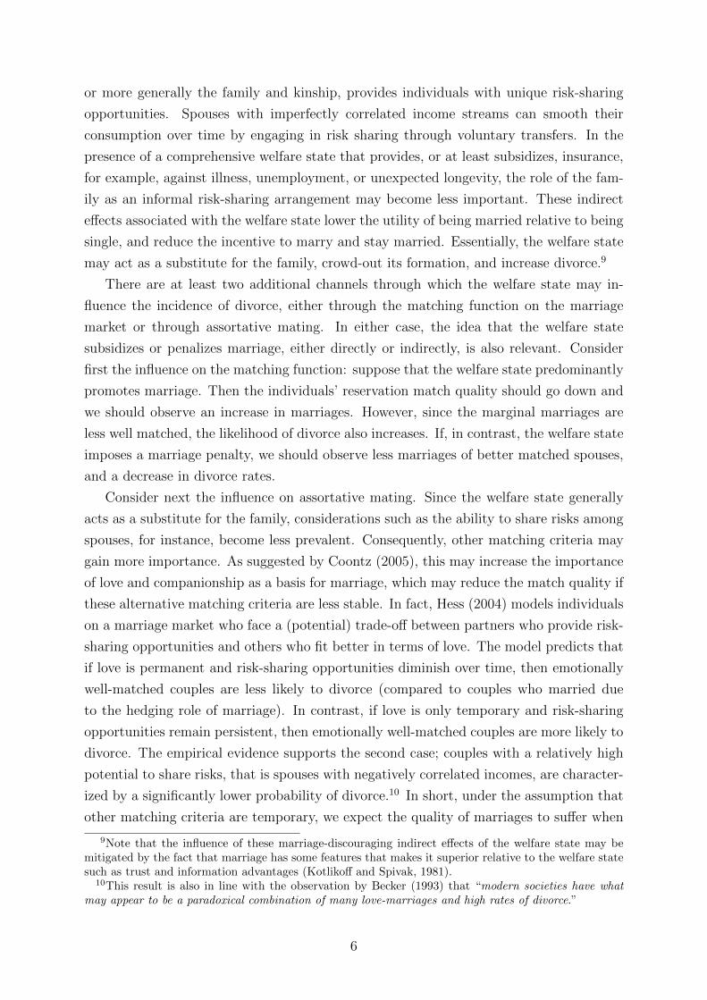
or more generally the family and kinship, provides individuals with unique risk-sharing

opportunities. Spouses with imperfectly correlated income streams can smooth their

consumption over time by engaging in risk sharing through voluntary transfers. In the

presence of a comprehensive welfare state that provides, or at least subsidizes, insurance,

for example, against illness, unemployment, or unexpected longevity, the role of the fam-

ily as an informal risk-sharing arrangement may become less important. These indirect

e↵ects associated with the welfare state lower the utility of being married relative to being

single, and reduce the incentive to marry and stay married. Essentially, the welfare state

may act as a substitute for the family, crowd-out its formation, and increase divorce.9

There are at least two additional channels through which the welfare state may in-

fluence the incidence of divorce, either through the matching function on the marriage

market or through assortative mating. In either case, the idea that the welfare state

subsidizes or penalizes marriage, either directly or indirectly, is also relevant. Consider

first the influence on the matching function: suppose that the welfare state predominantly

promotes marriage. Then the individuals’ reservation match quality should go down and

we should observe an increase in marriages. However, since the marginal marriages are

less well matched, the likelihood of divorce also increases. If, in contrast, the welfare state

imposes a marriage penalty, we should observe less marriages of better matched spouses,

and a decrease in divorce rates.

Consider next the influence on assortative mating. Since the welfare state generally

acts as a substitute for the family, considerations such as the ability to share risks among

spouses, for instance, become less prevalent. Consequently, other matching criteria may

gain more importance. As suggested by Coontz (2005), this may increase the importance

of love and companionship as a basis for marriage, which may reduce the match quality if

these alternative matching criteria are less stable. In fact, Hess (2004) models individuals

on a marriage market who face a (potential) trade-o↵ between partners who provide risk-

sharing opportunities and others who fit better in terms of love. The model predicts that

if love is permanent and risk-sharing opportunities diminish over time, then emotionally

well-matched couples are less likely to divorce (compared to couples who married due

to the hedging role of marriage). In contrast, if love is only temporary and risk-sharing

opportunities remain persistent, then emotionally well-matched couples are more likely to

divorce. The empirical evidence supports the second case; couples with a relatively high

potential to share risks, that is spouses with negatively correlated incomes, are character-

ized by a significantly lower probability of divorce.10 In short, under the assumption that

other matching criteria are temporary, we expect the quality of marriages to su↵er when

9Note that the influence of these marriage-discouraging indirect e↵ects of the welfare state may bemitigated by the fact that marriage has some features that makes it superior relative to the welfare statesuch as trust and information advantages (Kotliko↵ and Spivak, 1981).

10This result is also in line with the observation by Becker (1993) that “modern societies have whatmay appear to be a paradoxical combination of many love-marriages and high rates of divorce.”

6

extensive welfare state arrangements exist.

To summarize, in a welfare state that penalizes marriages, the direct and indirect

e↵ects of an expansion in the welfare state work in the same direction. Thus, we unam-

biguously expect a lower incidence of marriage and a higher incidence of divorce.11 In

contrast, in a welfare state setting that promotes marriage, the e↵ect of an expansion

is unclear. If the marriage-promoting direct e↵ect dominates the indirect e↵ect, the in-

cidence of marriages should go up, and the number of divorces down. Whereas if the

indirect e↵ect is more important than the direct e↵ect, we expect marriages to decrease

and divorces to increase. In the latter case, the e↵ect may be reinforced by a lower match

quality of marginal marriages and less-stable assortative mating patterns.

The e↵ect on fertility is also a priori ambiguous and depends on whether any direct

subsidy e↵ects are strong enough to compensate for the negative indirect e↵ects, such

as reduced incentives to have children being associated with extensive public pension

systems. Finally, an extension in the welfare state should increase the incidence of out of

wedlock births (marriage becomes less important for child care under an extensive welfare

state), unless the welfare state has pronounced subsidies for marital birth.

In the next section we discuss how we aim to empirically identify the e↵ect of the overall

impact of the welfare state on aggregate demographic trends—reflecting the potential

changes in family behavior discussed above.

3 Empirical Strategy and Data

Our discussion of a potential e↵ect of the welfare state on aggregate demographic trends

translates into a regression framework of the following type:

Di,t

= ↵r

·WSi,t

+X

i

�i

· Countryi

+X

t

�t

· Yeart

+ � ·Xi,t

+ "i,t

, (1)

where the dependent variable Di,t

captures di↵erent demographic outcomes in country

i in year t: either the incidence of marriage, divorce, or fertility. In the latter case, we

distinguish between total fertility, marital fertility, and non-marital fertility. We also

consider the ratio of children born out of wedlock as an additional outcome. The variable

WSi,t

denotes a proxy for the extent of the welfare state, and �i

and �t

denote country and

year fixed-e↵ects. In our baseline specification, we include a set of covariates Xi,t

, that

comprise the sex-age distribution, the prevalent abortion law, the prevalent divorce law

regime, the government’s ideological orientation and the degree of polarization. The sex-

age distribution is captured by 24 variables measuring the share of the total population

of sex s in age group a where a is 0-14, 15-19, . . . , 60-64, 65+. The abortion law regime is

11Marginal marriages may have in this situation a lower divorce likelihood due to a comparable highermatch quality.

7

captured by a binary variable equal to one if abortion is legal (Bellido and Marcen, 2014),

and zero otherwise. Regarding the divorce law, we distinguish between four regimes: (i)

divorce is not possible at all, (ii) where only at-fault divorce is possible, (iii) where a

no-fault divorce is available if both spouses agree; mutual consent divorce, and (iv) where

a no-fault divorce is also available if only one spouse requests this; unilateral divorce. The

coding is based on (Gonzalez and Viitanen, 2009) and some national sources in the case of

non-European countries.12 The control variables capturing the government’s ideological

orientation and the degree of polarization will be discuss below. In further specifications,

we will expand our set of covariates to control for macroeconomic conditions, the share

of immigrants, and the taxation of singles versus families. We calculate robust standard

errors throughout.13

3.1 Measuring Demographic Trends

The standard in the literature to quantify the incidence of marriage and divorce seems to

be crude marriage and divorce rates: the number of marriages (divorces, respectively) per

1,000 of the total population (e. g. Friedberg, 1998; Wolfers, 2006). While this approach is

potentially problematic, since it does not properly consider the population “at risk,” and

may therefore hide some of the underlying variation of interest, data restrictions impede

better approaches in most situations. In the case of marriage, the best measure would be

the ratio of the number of marriages in a given year to the stock of the non-married adult

population.14 In order to quantify the incidence of divorce, one would prefer to calculate

the ratio of the number of divorces in a given year to the stock of the married population.

Unfortunately, the stock of (non-)married people is not available for the majority of the

country-years; exceptions are the years in which a population census was conducted. As

a second-best solution, we calculate the marriage rate, Mi,t

, and the divorce rate, Di,t

,

based on the number of cases per 1,000 of the population between 15 and 64 years of age

(henceforth adults).

To measure fertility, the literature discusses cohort and period indicators. Cohort

indicators evaluate the birth rate of women born in a given year as they attain the

12The U.S. is the only country with within-country variation in divorce law (i.e. states switched tomutual consent divorce law and unilateral divorce law in di↵erent years). For the analysis, we imputethe median-introduction years for the U.S.

13Due to the relatively small number of countries (we have 21 to 23 countries in our data set) we donot cluster the standard errors in our baseline specification. Since standard cluster adjustment relies onthe assumption that the number of clusters approaches infinity, clustering may do more harm than goodin the case of few clusters. Nevertheless, we report our main results based on two di↵erent alternatives ofclustered standard errors in Section B.1 of the Web Appendix. In Table B.1 standard errors are clusteredby country. Here, standard errors increase on average by a factor of two. However, these estimates haveto be interpreted with extreme caution; due to the small number of clusters. In Table B.2 standard errorsare clustered by country and electoral cycles. This results in 175 to 185 clusters, which coincide with thelevel at which our instrumental variable mainly varies. Here, standard errors increase on average only bya factor of 1.3.

14Alternatively, one could also argue that married people are at risk to divorce and re-marry.

8

end of their reproductive cycle, while period indicators asses the rate of birth to women

of di↵erent ages in a given year, and implicitly assume that they behave according to

hypothetical schedules of specific cohorts. Though cohort indicators are clearly more

precise, the literature usually uses period indicators, since they are easily available and

allow examination of recent changes (d’Addio and d’Ercole, 2005). We employ the most

commonly used period indicator, the birth rate, which represents the absolute number of

births (to either all, married, or unmarried mothers) per 1,000 women of child-bearing

age. Information on births by mothers’ marital status is available for comparably less

country-years. See the Data Appendix for more information.15

3.2 Measuring the Extent of the Welfare State

To quantify the extent of the welfare state, we mainly use public social spending as a

percentage of GDP. Averaged across OECD member countries, total public social spend-

ing increased from 17.6 percent of GDP in 1980 to 21.4 percent in 2007 (see Figure 1).

Since the launch of the OECD Public Social Expenditure Database in 1980, this quan-

tity is consistently measured for all OECD member countries and captures expenditure

categories such as old age, health, incapacity-related benefits, family, unemployment, sur-

vivors, active labor market policies, and other (including housing).16 In each category,

public social spending comprise cash benefits, direct “in-kind” provision of goods and

services, and tax breaks with social purposes.17 On average, cash benefits account for

61.8 percent of total public social spending. Although, this relation has been relatively

stable over time, a slight decrease can be observed since the early 1990s. For further

information, see OECD (2007). Quantitatively the most important functional categories

are old age, health, incapacity-related benefits, and family benefits. This composition is

quite stable across countries and over time (see Section B.2 of the Web Appendix). That

means that our estimates provide a stable and interpretable marginal e↵ect of a typical

change in the size of the welfare state.

[ Insert Figure 1 about here ]

To check the robustness of our results, we use two alternative measures of the size of

the welfare state, a wider measure and a narrower measure. First, we use the size of the

15For a large sub-sample, we have the total fertility rate (TFR) available. While TFR is a preferredmeasure, since it is not a↵ected by the age distribution of the population, it does not allow us to distin-guish between marital and non-marital fertility. For the overall fertility rate we find based on the TFRquantitatively very comparable results (see below).

16OECD also provides information on public social spending before 1980; however, there is (as Figure1 shows) an obvious break in the series.

17Tax breaks intended to support married couples are not considered to serve a “social purpose”, andare therefore not included in the calculations (regardless of whether or not such measures are part of thebasic tax structure). Thus, the category “family” will capture only the e↵ect of the welfare state and notthe e↵ect of the tax law (on family behavior).

9

government sector as measured by total public spending as a percentage of GDP. This

series is available since 1970 (see Figure 1). Given that the size of the government sector

is clearly very broad and includes spending items that may be only remotely related to

family behavior, one may expect a weaker e↵ect. Second, we use public social spending

on the family as a percentage of GDP. This series is available since 1980 (see Figure

1). This subcategory of total public social spending comprises welfare state arrangements

directly related to families, such as child allowances and credits, child-care support, income

support during leave, and sole parent payments. Public social spending on the family has

increased (averaged across OECD member countries) from 1.7 percent of GDP in 1980 to

2.2 percent in 2007; this is equal to an increase of about 30 percent.

Note that although total public spending is available since 1970, we still focus on the

data from 1980 to 2007 in our main analysis since this sample guarantees comparability

of the estimation results across measures.18 In Section 4.3, we briefly report on the results

based on the longer sample.

3.3 Endogeneity of the Size of the Welfare State

The size of the welfare state may be endogenous in equation (1) for at least two reasons.

First, causality may run from existing or evolving family outcomes to the size of the

welfare state. For instance, the welfare state may have expanded to compensate for

declining marriage rates and provide services no longer provided within families. For

instance, Edlund and Pande (2002); Edlund, Haider and Pande (2005) argue that the

decline in marriage has increased the demand for redistribution by females (resulting in a

political gender gap), which increased the size of the welfare state. In this case, changing

family formation patterns causally a↵ect the size of the welfare state. Second, there may

have been changes in other observable or unobservable factors— such as changes in (sex-

specific) economic opportunities, in the organization of the marriage market, or in social

norms—a↵ecting the incentive to form or dissolve a family that are also correlated with

the extent of the welfare state.

It is hard to determine the sign of the potential bias, as it depends on the correlation

between the welfare state and the confounding factor(s) after partialing out the covariates

(such as country fixed e↵ects). Consider, for instance, a temporary historical shock to

fertility. If this shock results in a higher demand for welfare spending in the present,

then there will be a negative covariance between the transformed key regressor (after

18Table B.3 in the Web Appendix shows the values of each of our measures of the welfare state inthe first year for which we have an observation. We see that the initial size of the welfare state variesstrongly across countries regardless of which proxy we use. Initial public social spending varies from 9.92percent of GDP in Portugal to 27.16 percent in Sweden. Public spending on the family amounted to only0.47 percent of GDP in Spain, whereas it was 3.09 percent in Sweden, in the first year. Public spending,the broadest category we consider, ranges from to 29.25 percent of GDP in Greece to 62.78 percent inSweden.

10

eliminating country fixed e↵ects) and the transformed error term. This would gives rise

to a downward bias in the estimated coe�cient.

3.4 Political Fractionalization as a Source of Exogenous Varia-

tion

To allow for a causal interpretation, we adopt an instrumental variable strategy to isolate

exogenous variation in the size of the welfare state. We suggest to instrument WSi,t

in

equation (1) by a measure of political fractionalization, which refers to the number of

relevant parties involved in policy decisions. The choice of this instrumental variable

is motivated by the political economy theories of public finance. According to the so-

called common pool theory, highly fractionalized systems are prone to increase spending

since individual groups do not fully internalize the costs (see e.g. Weingast, Shepsle and

Johnsen, 1981; Velasco, 2000). The larger the number of parties involved—that is, the

more fractionalized the system—the stronger is the incentive to over-spend. Note that the

use of the terms fractionalization and fragmentation is not unambiguous in the literature.

Although it usually refers to the number of parties participating in fiscal policy decision

making, it is also used to describe the ideological coherence of groups involved in policy

making (see Volkerink and de Haan, 2001).

Primo and Snyder (2008), in contrast, argue that fractionalization may lead to lower

spending, especially with respect to total public spending. Intuitively, suppose that legis-

lators have a choice of one large project that benefits all groups to some extent, or several

small projects where each project benefits only an individual group. Even though the

large and more expensive project might be more appropriate, individual groups may push

for smaller and cheaper projects that allow them to internalize group-specific benefits to a

greater extent. In this case, total public spending can be lower, albeit each group pushes

for an ine�ciently expensive project.

The empirical evidence is also mixed. A number of studies (see e. g. Roubini and

Sachs, 1989,b; Persson and Tabellini, 2004, among others) find that more fragmented

governments lead to higher spending and deficits. However, as pointed out by Acemoglu

(2005), these results may be subject to a substantial endogeneity bias, which is typically

not addressed in a proper way.

Di↵erent measurements for party fractionalization exist. We use an index proposed by

Rae (1968) that focuses on the degree of legislative fractionalization of the party-system.

In particular, the Rae-Index is defined as 1�P

n

i=1 s2i

, where si

is the share of parliamen-

tary seats for party i and n is the number of parties. This means that a higher value of

the Rae-Index indicates a more fractionalized system. We find a very stable relationship

between legislative fractionalization and public spending in our data. The cross-sectional

correlation between the Rae-Index and the level of public spending is positive (see the

11

upper panel in Figure 2). Hence, it appears that a more fragmented legislative is asso-

ciated with higher public spending. This relation also holds in a regression framework

(with a large set of covariates).19 However, if we augment the regression equation with

country fixed-e↵ects—which account for unobserved time-invariant heterogeneity—the

estimated coe�cient is still highly significant, albeit with a negative sign (see the lower

panel in Figure 2). Here, a one standard deviation increase in the Rae-Index decreases

public spending by 0.4 standard deviations. Importantly, the same patterns are observ-

able for public social spending, which is our main proxy for the size of the welfare state,

as well as for public social spending on the family. Here the beta coe�cients change

due to the inclusion of country fixed-e↵ects from 0.5 to �0.3, and from 0.4 to �0.1, re-

spectively. These results suggest that the degree of party fractionalization is correlated

with unobserved country-specific time-invariant heterogeneity in a way that disregarding

country fixed-e↵ects can diametrically reverse results. Clearly, the model with country

fixed-e↵ects is superior, and we conclude that a higher degree of legislative fractional-

ization in the party system leads to lower public (social) spending in OECD member

countries. While older empirical contributions put forward a positive relationship, re-

lying on di↵erent data sets and estimation methods, our finding is consistent with the

theoretical prediction of Primo and Snyder (2008).


Note, however, whether a higher degree of fractionalization increases or decreases

public social spending does not a↵ect the validity of our key identifying assumptions.

We presume that the number of relevant political parties involved in the parliament is

not correlated with unobserved factors determining family behavior. In other words,

our measure of political fractionalization must a↵ect family behavior only through the

channel of public social spending. Thus, political fractionalization can be excluded from

the second-stage regression displayed in equation (1).

While this identifying assumption is not testable, it is instructive to discuss the source

of variation in the degree of fractionalization. The Rae-Index changes either due to

changes in popular support in elections, or due to institutional reforms that change the

parliamentary representation of parties given their popular support. Empirically we can-

not distinguish these two sources of variation, since such reforms typically become e↵ective

in election years. In our estimation sample about 98 percent of the changes in the Rae-

Index take place in election years; i. e. the institutional reforms are essentially collinear

with elections. The important question is, however, whether such institutional reforms

or changes in popular support are correlated with unobserved factors determining family

19For instance, a regression of public spending on the Rae-Index and year fixed-e↵ects suggests that anincrease in the Rae-Index by one standard deviation increases public spending by 0.4 standard deviation.The estimated coe�cient is significant at the 1-percent level.

12

behavior. While we regard the former correlation as highly improbable, we think the

latter relation requires an in-depth discussion. It appears conceivable that changes in the

Rae-Index driven by changes in popular support coincide with changes in overall values

and social norms, which could be directly related to our outcome variable. For instance,

if changes in the fractionalization tend to coincide with shifts from left to right-wing

governments (or vice versa), then our instrumental variable may be correlated with unob-

served governments’ characteristics that also a↵ect family outcomes. In fact, we find some

correlations between the Rae-Index and the government’s ideological orientation. While

the inclusion of respective control variables does not alter our estimation results, we in-

clude the share of cabinet posts held by left-wing, center, and right-wing parties (each

weighted by days) as control variables in our baseline specification; where share of cabinet

posts held by right-wing parties (and independents) serves as base group. Equivalently,

one might speculate about a link between polarization within the government and family

behavior. We use a three-valued indicator to measure polarization in the government

in our baseline specification.20 Again, controlling for polarization does not change our

results. Another mediating link (i. e., variable that is potentially correlated with political

fractionalization and family behavior) we can think of is immigration. For whatever rea-

sons, more (or less) fractionalized governments may have a di↵erent immigration policies;

which in turn might a↵ect family behavior. Again, our results are robust to the inclusion

of the share of immigrants. Finally, one might be concerned about the potential influence

of demographic variables on political outcomes. Alesina and Giuliano (2011) show, for

instance, that family ties influence political participation. However, although the family

and political outcomes may be interlinked in general, it is unclear how family ties a↵ect

fractionalization of the government.

Before we turn to the discussion of our estimation results it should be noted that based

on our instrumental variable approach, we are able to measure the impact of marginal

changes in the extent of the welfare state (due to variation in the political fractionalization)

at the intensive margin. It is unclear whether a variation at the extensive margin (i. e.,

the introduction of a welfare state) has the same e↵ect on the formation and dissolution

of families.20A government is least polarized (41.8 percent of our observations) if it consists only of either left-

wing, center, or right-wing parties. It is most polarized if it consists of both left and right-wing parties(33.3 percent). Medium polarized governments are a mix of left-wing and center parties or right-wingand center parties (24.9 percent). We include binary indicators to capture these three levels.

13

4 Estimation Results

4.1 Main Results

Table 1 presents the main results of this paper, where we use public social spending to

capture the size of the welfare state.21 To facilitate an easier interpretation of the quan-

titative importance of our estimation results, we provide in the upper panel besides the

coe�cients and the standard errors also semi-elasticities (using the unweighted mean as

the base) and standardized (beta) coe�cients. For comparison, we also report correspond-

ing OLS estimates. The lower panel summarizes our first stage results. The Rae-Index

is highly significantly negative in all specifications and the Kleibergen-Paap F-statistic

indicates that the Rae-Index is not a weak instrument.

[ Insert Table 1 about here ]

The first three columns show that an expansion in the welfare state increases the

incidence of marriage, divorce, and fertility. The extent of the welfare state is not only a

statistically significant but also a quantitatively important predictor of these rates. The

estimates imply that an increase in public social spending by one percentage point of GDP

increases the marriage rate by 2.4 percent, the divorce rate by 3.9 percent, and the fertility

rate by 2.1 percent. This is equivalent to the beta coe�cients of approximately 0.5, 0.4,

and 0.5, respectively. Interestingly, endogeneity seems to play a more important role in

the case of marriage and fertility. Here, OLS and instrumental variable estimates are

even of opposite signs, whereas in the case of divorce, both estimators provide the same

qualitative conclusion. Comparing the point estimates shows that the OLS estimates are

downward biased in the case of each outcome.

These results suggest that welfare state regulations contain a strong marriage-promoting

component (direct e↵ect) that overcompensates any crowding-out due to substitutabil-

ity between the family and the welfare state (indirect e↵ect). An equivalent relationship

seems to hold between the welfare state and overall fertility. Thus, the welfare state clearly

promotes the formation of families. However, at the same time, a larger welfare state also

facilitates the dissolution of families. The positive e↵ect on the incidence of divorce may

result from di↵erent causal channels. First, a more pronounced welfare state may fa-

cilitate divorce by providing or subsidizing goods and services to divorced spouses that

would be otherwise only available within marriage (e.g., risk sharing). Put di↵erently, in

the case of divorce, the indirect e↵ect may dominate the direct e↵ect. Second, marginal

marriages—those which would have not been formed without the marriage-promoting

21We use the subset of 570 country-years with non-missing information on the marriage, divorce, andoverall fertility rates in the first three columns. In the remaining three columns, we use the 538 country-years with information on fertility rates by marital status.

14

component of the welfare state—may have a lower match quality, which increases mar-

ital instability. Third, the welfare state may alter assortative mating patterns such that

less stable marriages are formed.22

Given that our measurements of the incidence of marriage and divorce are both flow

measurements, our results allow the interpretation that a large welfare state increases

activity in the marriage market. This result is in line with the theoretical predication

by Anderberg (2007). A larger welfare state seems to facilitate the transitions between

di↵erent family status. This result seems plausible since such transitions are usually

associated with high cost and uncertainty. Comparing the two estimated coe�cients, we

see that the flow into marriage (plus 210 marriages per 1,000 adults) is higher than the

flow out of marriage (plus 118 divorces per 1,000 adults). Thus, the overall e↵ect of an

expansion of the welfare state on the stock of married people is positive.23

The result that countries characterized by extensive welfare states tend to have higher

fertility rates is consistent with the interpretation that the welfare state increases the

demand for children (crowding-in e↵ect), for instance, by subsidizing children via benefits

or tax deductions.24 This direct e↵ect seems larger than any negative indirect e↵ect. A

more detailed investigation of fertility patterns shows that an expansion of the welfare

state also alters the distribution of births in and out of wedlock. The fourth and fifth

columns show that an expansion of the welfare state increases fertility rates among married

mothers (1.6 percent) and non-married mothers (3.9 percent). Despite the fact that an

expansion increases the incidence of marriage—and therefore, increases the population

at risk for married fertility—we observe a comparably larger relative increase in out-of-

wedlock births. This is also reflected in the final column, where we see that an increase

in public social spending by one percentage point of GDP increases the share of children

born out of wedlock by approximately 0.7 percentage points. This finding is consistent

with the view that the welfare state creates incentives by providing higher support for

single mothers (direct e↵ect, as for instance in the case of AFDC), and with the idea that

the welfare state acts as a substitute for a stable union (indirect e↵ect).

22In principle, it is possible that the increased incidence of divorce drives some of the positive e↵ect onthe marriage rate (i.e., divorces increase the supply of potential partners in the marriage market). Thiscould be tested with data on first (and further) marriages. However, this information is not available forthe majority of country-years. Similarly, data on demographic outcomes by age or cohort would enablefurther tests; but these are hardly available.

23A more direct test of the e↵ect of the welfare state on the stock of married population, would be touse the stock of married population as an outcome variable. However, due to limited data availability,such an analysis is not feasible for a large panel of countries. The stock of population by family status isusually only available for the census years.

24Table B.4 in the Web Appendix summarizes estimation results based on the TFR. We obtain thesame qualitative results. A comparison of the respective beta coe�cients shows that the e↵ects are largerwhen using the TFR.

15

4.2 Alternative Measurements of the Welfare State

While we rely on public social spending to measure the size of the welfare state in our

main analysis, we find very comparable results for public social spending on the family

(see Table 2) and public spending (see Table 3); both spending variables are measured as a

percentage of GDP. Using public social spending on the family has the advantage that it is

the most narrowly defined spending category and contains spending that is closely related

to families. Given this close link to family formation and dissolution, we expect larger

e↵ects with this spending category. Nevertheless, relating public spending categories to

family formation and family structure remains a complicated task. For instance, public

expenditure on education is included in public spending, but not in public social spending

(on the family). Since education spending is presumably an important determinant of

family structure, we also look at public spending as a broader measure of the welfare

state.

[ Insert Tables 2 and 3 about here ]

We see from Tables 2 and 3 that the same qualitative conclusions emerge regardless of

the proxy for the size of the welfare state. Using public social spending on the family, the

magnitudes of the e↵ect of the welfare state generally increase as beta coe�cients roughly

double. Note, that in the case of the martial fertility rate the standard errors increase

and the e↵ect is no longer significant at conventional levels.25 For public spending (the

broadest category), based on a strong first-stage regression, all e↵ects remain statistically

significant and magnitudes tend to be somewhat smaller.

Finally, we also used public social spending net of the category ‘old age’ as an al-

ternative measure of the size of the welfare state (see Table B.5 in the Web Appendix).

The idea is that family formation and dissolution is mainly driven by younger couples,

and should therefore not strongly (or, at least not directly) react to variation in spending

on pensions and other social services for the elderly people. As expected, we find the

same qualitative results, with generally larger, albeit less significant, quantitative e↵ects

as compared to the baseline specification. It has to be noted, however, that these results

have to be interpreted with some caution as the Kleibergen-Paap F-statistics are only

between six and seven.

4.3 Sensitivity Analysis

To check the robustness of our results, we ran a number of alternative specifications.

The results are summarized in Figure 3, where the panels are organized by the di↵erent

25Relatedly, the Kleibergen-Paap F-statistics are generally only about eight.

16

outcome variables.26 Each panel also shows the respective estimates from the baseline

specifications.


First, we use the first lag of public social spending instead of the contemporaneous

value. We see that the e↵ects on the marriage, divorce, and fertility rates are rather

similar to our baseline specification. Second, we augment the specification with the real

GDP growth rate as the overall-level economic activity may also have a potential impact

on demographic outcomes (see, e. g., Hellerstein and Morrill, 2011). We obtain highly

similar results. Third, we include the share of immigrants as an additional covariate. As

discussed earlier, immigration is a potential confounding factor, since it may be correlated

with fractionalization and demographic outcomes. We again obtain similar results.27

Fourth, we augment the baseline specification with controls for family related taxation.

In particular, we include a measure of the average income tax rate for (i) a single with

no child, and (ii) a married couple with two children.28 While explicitly controlling for

taxation renders the e↵ects insignificant for divorce and for the wedlock ratio, overall, our

results remain robust.

We also examine the robustness of our results with respect to the sample chosen. First,

we checked whether our results are driven by observations from countries with a certain

electoral system. Therefore, we exclude all countries (about 23 percent of the sample)

characterized by a majority voting system according to Blaise and Massicotte (1997). Our

overall results, remain robust in these estimations (see Table B.6 in the Web Appendix).

It is reassuring that our results are not strongly influenced by how popular vote is mapped

into parliamentary representation.

Second, we examined longer sample periods since the data on public spending and

public social spending are available since 1970.29 With the longer series, we obtain the

same qualitative results for both measurements, although the e↵ects are less precisely

estimated (see Tables B.7 and B.8 in the Web Appendix). Quantitatively, we observe a

small increase (across all outcomes) in the case of public social spending, while we see

some comparably smaller e↵ects for public spending. Finally, we account for the fact

that the Rae-Index hardly varies in between elections by aggregating our data to election

cycles, which results in about 180 observations. For all other variables we generate their

26For our two alternative measurements we performed the same set of alternative specifications. TheFigures B.1 and B.2 in the Web Appendix show that also these results are qualitatively robust.

27The best available data on the number of foreign-born population we are aware of is included in theWorld Development Indicators Database provided by the World Bank. Since information is only availablefor every fifth year, we linearly interpolated the series to impute for missing years.

28These estimated average tax rates are taken from the OECD Taxing Wages Database, which presumesfor the single, earnings of 67 percent of the average production worker wage, and for the married couplea principal earner with 100 percent and spouse with 33 percent of the average production worker wage.Some missing values have been imputed by linear interpolation.

29A caveat is that the public social spending series show a break in 1980.

17

within spell-mean.30 Table B.9 in the Web Appendix summarizes estimations based on

this aggregated data equivalent to our baseline specifications. Despite the smaller sample,

we observe again qualitatively very comparable results.

5 Concluding Remarks

Based on country-level data from OECD member countries from the past three decades,

we conclude that a larger welfare state increases the turn-over in the marriage market.

Since the e↵ect on the incidence of marriage dominates the e↵ect on divorce, the stock

of married population increases. In addition, a larger welfare state also raises overall

fertility. Thus, the welfare state supports the formation of families on an aggregated

level. Yet, we find that the welfare state crowds-out the traditional organization of the

family. The comparable stronger impact on non-marital fertility (compared to marital

fertility) increases the share of children born out of wedlock.

This can be explained by the economic theory of the family, which also partly corrobo-

rates earlier results. It is consistent with the interpretation that the average welfare state

in OECD member countries entails a positive direct e↵ect that outweighs any negative in-

direct e↵ect. The positive e↵ect on divorce may result from a reduction in the (economic)

cost of divorce by improvements in the post-divorce income situation (for average and

marginal marriages). Put di↵erently, the welfare state facilitates the formation and the

dissolution of families. Whether these family transitions (triggered by the welfare state)

are welfare enhancing or not, cannot be answered and remains an open question. How-

ever, since the welfare state reduces the cost of divorce, it seems plausible that surviving

marriages are of better quality and exhibit higher marital satisfaction. Consequently, we

would expect a lower level of extreme forms of marital distress in countries with a larger

welfare state.31

As in the case of every instrumental variable estimation, some uncertainty about

the validity of the exclusion restriction may remain, since the identifying assumption is

fundamentally untestable. While we hope that our discussion and the robustness checks

have convinced the reader, we would propose for further research to use other sources of

exogenous variation to test our hypotheses if any opportunity arises.

To which degree can our findings be generalized? A final caveat of instrumental vari-

able estimations is that they provide only a local average treatment e↵ect. In particular,

our estimation captures the e↵ect of a change in the extent of the welfare state due to a

30Since our measures of the size of the welfare state vary between elections, aggregation to electioncycles entails a loss of information. The disaggregated analysis above exploits this in-between electionsvariation.

31Along similar lines, Stevenson and Wolfers (2007) argue that the introduction of unilateral divorcelaw, which can also be interpreted as a reduction in the cost of divorce, substantially reduced femalesuicide, domestic violence (for both men and women), and females murdered by their partners.

18

varying degree of political fractionalization. While it is generally hard to assess the ex-

ternal validity, it seems attractive that our estimation relies on data from a broad range

of OECD countries, comprising a variety of di↵erent programs which were implemented

at di↵erent points in time.

19

References

Acemoglu, D. (2005). Constitutions, Politics, and Economics: A Review Essay onPersson and Tabellini’s The Economic E↵ects of Constitutions. Journal of EconomicLiterature, 43 (4), 1025–1048.

Akerlof, G. A., Yellen, J. L. and Katz, M. L. (1996). An Analysis of Out-of-Wedlock Childbearing in the United States. Quarterly Journal of Economics, 111 (2),277–317.

Algan, Y. and Cahuc, P. (2009). Civic Virtue and Labor Market Institutions. Amer-ican Economic Journal: Microeconomics, 1 (1), 111–145.

Alesina, A. and Giuliano, P. (2011). Family Ties and Political Participation. Journalof the European Economic Association, 9 (5), 817–837.

Alm, J., Dickert-Conlin, S. and Whittington, L. A. (1999). Policy Watch: TheMarriage Penalty. Journal of Economic Perspectives, 13 (3), 193–204.

Anderberg, D. (2007). Marriage, Divorce and Reciprocity-based Cooperation. Scandi-navian Journal of Economics, 109 (1), 25–47.

Becker, G. S. (1973). A Theory of Marriage: Part I. Journal of Political Economy,81 (4), 813–846.

— (1974). A Theory of Marriage: Part II. Journal of Political Economy, 82 (2), 11–26.

— (1993). A Treatise on the Family, Enlarged Edition. Cambridge, MA: Harvard Univer-sity Press.

—, Landes, E. M. and Michael, R. T. (1977). An Economic Analysis of MaritalInstability. Journal of Political Economy, 85 (6), 1141–1187.

Bellido, Hector and Marcen, Miriam (2014). Divorce Laws and Fertility. LabourEconomics, 27 (1), 56–70.

Bjorklund, A. (2006). Does Family Policy A↵ect Fertility? Journal of PopulationEconomics, 19 (1), 3–24.

Blais, Andre and Massicotte, Louis (1997). Electoral Formulas: A MacroscopicPerspective. European Journal of Political Research, 32 (1), 107–129.

Blank, R. M. (2002). Evaluating Welfare Reform in the United States. Journal ofEconomic Literature, 40 (4), 1105–1166.

Brotherson, S. E. and Duncan, W. C. (2004). Rebinding the Ties That Bind: Gov-ernment E↵orts to Preserve and Promote Marriage. Family Relations, 53 (5), 459–468.

Castles, F. G., Leibfried, S., Lewis, J., Obinger, H. and Pierson, C. (eds.)(2010). The Oxford Handbook of the Welfare State. Oxford: Oxford University Press.

Cigno, A. (1986). Fertility and the Tax-Benefit System: A Reconsideration of the Theoryof Family Taxation. Economic Journal, 96 (384), 1035–1051.

20

Coontz, S. (2005). Marriage, A History: From Obedience to Intimacy, or How LoveConquered Marriage. New York: Viking.

d’Addio, A. C. and d’Ercole, M. M. (2005). Trends and Determinants of Fertil-ity Rates in OECD Countries: The Role of Policies. OECD Social, Employment andMigration Working Paper 27, OECD, Paris.

Edlund, L., Haider, L. and Pande, R. (2005). Unmarried Parenthood and Redis-tributive Politics. Journal of the European Economic Association, 3 (1), 95–119.

— and Pande, R. (2002). Why Have Women Become Left-Wing? The Political GenderGap and the Decline in Marriage. Quarterly Journal of Economics, 117 (3), 917–961.

Friedberg, L. (1998). Did Unilateral Divorce Raise Divorce Rates? Evidence fromPanel Data. American Economic Review, 88 (3), 608–627.

Gardiner, K. N., Fishman, M. E., Nikolov, P., Glosser, A. and Laud, S.(2002). State Policies to Promote Marriage – Final Report. Tech. rep., U.S. Depart-ment of Health and Human Services, Assistant Secretary for Planning and Evaluation,Washington, DC.

Goldin, C. and Katz, L. F. (2000). Career and Marriage in the Age of the Pill.American Economic Review, Papers & Proceedings, 90 (2), 461–465.

— and — (2002). The Power of the Pill: Oral Contraceptives and Women’s Career andMarriage Decisions. Journal of Political Economy, 110 (4), 730–770.

Gonzalez, L. (2007). The E↵ect of Benefits on Single Motherhood in Europe. LabourEconomics, 14 (3), 393–412.

Gonzalez, L. (2005). The Determinants of the Prevalence of Single Mothers: A Cross-Country Analysis. Institute for the Study of Labor (IZA) Discussion Paper 1677.

Gonzalez, L. and Viitanen, T. (2009). The E↵ect of Divorce Laws on Divorce Ratesin Europe. European Economic Review, 53 (2), 127–138.

Grogger, J. and Karoly, L. A. (2005). Welfare Reform: E↵ects of a Decade ofChange. Cambridge, MA: Harvard University Press.

Halla, M. (2013). The E↵ect of Joint Custody on Family Outcomes. Journal of theEuropean Economic Association, 11 (2), 278–315.

Hellerstein, K. H. (2011). Booms, Busts, and Divorce. The B.E. Journal of EconomicAnalysis & Policy: Contributions, 11 (1), Article 54.

Hess, G. D. and Sandler Morrill, M. (2011). Marriage and Consumption Insurance:What’s Love Got to Do with It? Journal of Political Economy, 112 (2), 290–318.

Hu, W. (2003). Marriage and Economic Incentives Evidence from a Welfare Experiment.Journal of Human Resources, 38 (4), 942–963.

Isen, A. and Stevenson, B. (2011). Women’s Education and Family Behavior: Trendsin Marriage, Divorce and Fertility. In J. Shoven (ed.), Demography and the Economy,Chicago, IL: University of Chicago Press.

21

Kleibergen, F. and Paap, R. (2006). Generalized Reduced Rank Tests Using theSingular Value Decomposition. Journal of Econometrics, 133 (1), 97–126.

Kotlikoff, L. J. and Spivak, A. (1981). The Family as an Incomplete AnnuitiesMarket. Journal of Political Economy, 89 (2), 372–391.

Lindbeck, A. and Nyberg, S. (2006). Raising Children to Work Hard: Altruism, WorkNorms, and Social Insurance. Quarterly Journal of Economics, 121 (4), 1473–1503.

—, — andWeibull, J. W. (1999). Social Norms and Economic Incentives in the WelfareState. Quarterly Journal of Economics, 114 (1), 1–35.

Matouschek, N. and Rasul, I. (2008). The Economics of the Marriage Contract:Theories and Evidence. Journal of Law and Economics, 51 (1), 59–110.

Moffitt, R. A. (1992). Incentive E↵ects of the U.S. Welfare System: A Review. Journalof Economic Literature, 30 (1), 1–61.

— (1997). The E↵ect of Welfare on Marriage and Fertility: What Do We Know andWhat Do We Need to Know? Discussion Paper 1153, Institute for Research on PovertyDiscussion, University of Wisconsin.

— (1998). The E↵ects of Welfare on Marriage and Fertility. In R. A. Mo�tt (ed.),Welfare,the Family, and Reproductive Behavior, Washington, D.C.: National Research Council.

Murray, C. (1993). Welfare and the Family: The U.S. Experience. Journal of LaborEconomics, 11 (1).

Nechyba, T. J. (2001). Social Approval, Values, and AFDC: A Reexamination of theIllegitimacy Debate. Journal of Political Economy, 109 (3), 637–672.

OECD (2007). The Social Expenditure Database: An Interpretive Guide SOCX 1980-2003. Interpretative Guide of SOCX, OECD, Paris.

— (2011). Public Social Spending. In OECD, Society at a Glance 2011: OECD SocialIndicators, Paris: OECD Publishing.

Persson, T. and Tabellini, G. (2004). Constitutional Rules and Fiscal Policy Out-comes. American Economic Review, 94 (1), 25–45.

Pettersson-Lidbom, P. (2012). Does the Size of the Legislature A↵ect the Size ofGovernment? Evidence from Two Natural Experiments. Journal of Public Economics,96 (3), 269–278.

Primo, D. M. and Snyder, J. M. (2008). Distributive Politics and the Law of 1/n.Journal of Politics, 70, 477–186.

Rae, D. (1968). A Note on the Fractionalization of Some European Party Systems.Comparative Political Studies, 1 (3), 413–418.

Rasul, I. (2006). Marriage Markets and Divorce Laws. Journal of Law, Economics andOrganization, 22 (1), 30–69.

22

Roubini, N. and Sachs, J. D. (1989). Government Spending and Budget Deficits inthe Industrial Countries. Economic Policy, 4 (8), 100–132.

— and — (1989b). Political and Economic Determinants of Budget Deficits in the In-dustrial Democracies. European Economic Review, 33 (5), 903–933.

Stevenson, B. and Wolfers, J. (2007). Bargaining in the Shadow of the Law: DivorceLaws and Family Distress. Quarterly Journal of Economics, 121 (1), 267–288.

Stevenson, B. and Wolfers, J. (2007). Marriage and Divorce: Changes and theirDriving Forces. Journal of Economic Perspectives, 21 (2), 27–52.

U.S. General Accounting Office (2004). Defense of Marriage Act: Update to PriorReport. Tech. rep., Washington, DC.

Velasco, A. (2000). Debts and Deficits with Fragmented Fiscal Policymaking. Journalof Public Economics, 76 (1), 105–125.

Volkerink, B. and de Haan, J. (2001). Fragmented Government E↵ects on FiscalPolicy: New Evidence. Public Choice, 109 (3-4), 221–242.

Weingast, B. R., Shepsle, K. A. and Johnsen, C. (1981). The Political Economyof Benefits and Costs: A Neoclassical Approach to Distributive Politics. Journal ofPolitical Economy, 89 (4), 642–664.

Wolfers, J. (2006). Did Unilateral Divorce Laws Raise Divorce Rates? A Reconciliationand New Results. American Economic Review, 96 (5), 1802–1820.

23

6 Tables and Figures

Figure 1: Development of Public Spending Categoriesa

a This graph shows the development of pubic spending, public social spending, and public social spending on thefamily averaged across OECD member states from 1970 through 2007. Data on public social spending on the familyis only available since 1980. All public spending categories are measured as percentage of GDP. Further details areprovided in the Data Appendix.

24

Figure 2: Public Spending and Legislative Fractionalization in OECD MemberCountries (1980-2007)a

a These graphs show the relationship between public spending (measured as percentage of GDP) and the Rae-Indexof legislative fractionalization of the party-system. A higher value of the Rae-Index indicates a more fragmentedsystem. Further details are provided in the Data Appendix. The upper panel shows the simple cross-sectionalrelationship. The lower panel accounts (via demeaning) for country fixed e↵ects

25

Table

1:TheE↵ect

ofPublicSocialSpendingon

theForm

ation

and

Disso

lution

ofFamiliesa

Marital

Non-m

arital

Out-of-wedlock

Marriagera

teb

Divorcera

tec

Fertilityra

ted

fertilityra

tee

fertilityra

tef

ratiog

Publicsocial

spendingh

Coe�cienti

0.210**

0.118***

1.175***

0.662*

0.590***

0.677**

Standarderrorj

(0.089)

(0.031)

(0.411)

(0.371)

(0.221)

(0.309)

Sem

i-elasticity

k

[0.024]

[0.039]

[0.021]

[0.016]

[0.039]

[0.027]

Betacoe�

cientl

{0.530}

{0.393}

{0.471}

{0.322}

{0.287}

{0.215}

OLSestimate

-0.061***

0.051***

-0.154

-0.212**

0.006

-0.031

(0.020)

(0.008)

(0.102)

(0.099)

(0.068)

(0.107)

Con

trol

variab

lesm

Yes

Yes

Yes

Yes

Yes

Yes

Cou

ntry

andyear

fixed-e↵ects

Yes

Yes

Yes

Yes

Yes

Yes

No.

ofob

s./cou

ntries

570/23

570/23

570/23

538/21

538/21

538/21

Meanof

dep

endentvariab

le8.59

3.05

55.21

42.54

14.94

25.23

Sum

maryof

firststages:

Rae-Index

n

-0.103***

-0.103***

-0.103***

-0.108***

-0.108***

-0.108***

(0.018)

(0.018)

(0.018)

(0.020)

(0.020)

(0.020)

F-statistic

o

32.337

32.337

32.337

29.121

29.121

29.121

a

This

table

summarizesresu

ltsfrom

a2SLSestimationofth

ee↵

ectofpublicsocialsp

endingonmarriage,

divorceandfertilitybeh

avior.

Data

from

OECD-m

ember

countriesfrom

theyea

rs1980th

rough2007is

used.Note,someco

untry-yea

rsare

missing(see

Data

Appen

dix).

Theinstru

men

talvariable

iseq

ualto

theamea

sure

ofgovernmen

tfractionaliza

tion(see

below).

b

The

marriagerate

isth

eabsolute

number

ofmarriages

per

1,000ofth

epopulationbetween15and64yea

rs(h

enceforthadults).

c

Thedivorcerate

isth

eabsolute

number

ofdivorces

per

1,000

adults.

d

Thefertilityrate

isth

eabsolute

number

oflivebirth

sto

allfemalesper

1,000female

populationofch

ildbea

ringage(i.e.between15and44yea

rsofage).

e

Themaritalfertilityrate

isth

eabsolute

number

oflivebirth

sto

allmarriedfemalesper

1,000female

populationofch

ildbea

ringage.

f

Thenon-m

aritalfertilityrate

isdefi

ned

asth

eabsolute

number

oflivebirth

sto

all

unmarriedfemalesper

1,000female

populationofch

ildbea

ringage.

g

Theout-of-wed

lock

ratiois

defi

ned

asth

enumber

ofnon-m

aritalbirth

sdivided

byallbirth

smultiplied

by100.

h

Public

socialsp

endingis

mea

suredaspercentageofGDP.i

Listedco

e�cien

tsare

reported

asth

ech

angein

thesp

ecificrate

(ratio)dueto

anonepercentagepointincrea

sein

publicsocialsp

ending

mea

suredaspercentageofGDP.*,**and***indicate

statisticalsignifica

nce

atth

e10-percentlevel,5-percentlevel,and1-percentlevel,resp

ectively.

j

Robust

standard

errors

(allowingfor

heterosked

asticityofunknownform

)in

roundparenth

eses.k

This

semi-elasticity(calculatedusingth

eunweightedmea

nasth

ebase)multiplied

by100gives

thepercentagech

angein

thesp

ecific

rate

(ratio)dueto


sein

publicsocialsp

endingmea

suredaspercentageofGDP.l

This

standard

ized

(beta)co

e�cien

tgives

thestandard

dev

iationincrea

sein

the

specificrate

(ratio)dueto

aonestandard

dev

iationincrea

sesin

publicsocialsp

ending.

m

Each

specifica

tionco

ntrols

forth

egovernmen

t’sideo

logicalorien

tation,th

egovernmen

t’spolariza

tion,

theprevailingabortionlaw,th

edivorcelaw

regim

e,andth

esex-agedistribution.Thelatter

isca

ptu

redby24variablesmea

suringth

esh

are

ofth

etotalpopulationofsexsin

agegroupa

whereais

0�

14,15�

19,...,60�

64,65+.

n

TheRae-Index

(Rae,

1968)is

amea

sure

ofth

edeg

reeoflegislativefractionaliza

tionofth

eparty-system

;ahigher

valueofth

eRae-Index

indicates

amore

fragmen

tedsystem

.o

Kleibergen

-PaapF-statistic

(Kleibergen

andPaap,2006);

null-hypoth

esis

isth

atinstru

men

tis

wea

k.

26

Table

2:TheE↵ect


theFamilyon

theForm

ation

and

Disso

lution

ofFamiliesa

Marital

Non-m

arital

Out-of-wedlock

Marriagera

teb

Divorcera

tec

Fertilityra

ted

fertilityra

tee

fertilityra

tef

ratiog

Publicsocial

spend.on

thefamilyh

Coe�cienti

2.272**

1.320**

12.604**

6.297

7.227**

9.002**

Standarderrorj

(1.109)

(0.520)

(5.409)

(4.349)

(2.830)

(4.135)

Sem

i-elasticity

k

[0.265]

[0.432]

[0.228]

[0.148]

[0.483]

[0.356]

Betacoe�

cientl

{1.147}

{0.878}

{1.014}

{0.616}

{0.706}

{0.574}

OLSestimate

-0.176**

0.169***

0.419

-0.455

1.091***

0.041

(0.087)

(0.040)

(0.528)

(0.468)

(0.263)

(0.383)

Con

trol

variab

lesm

Yes

Yes

Yes

Yes

Yes

Yes

Cou

ntry

andyear

fixed-e↵ects

Yes

Yes

Yes

Yes

Yes

Yes

No.

ofob

s./cou

ntries

568/23

568/23

568/23

536/21

536/21

536/21

Meanof

dep

endentvariab

le8.59

3.05

55.19

42.52

14.96

25.26

Sum

maryof

firststages:

Rae-Index

n

-0.010***

-0.010***

-0.010***

-0.010***

-0.010***

-0.010***

(0.003)

(0.003)

(0.003)

(0.004)

(0.004)

(0.004)

F-statistic

o

8.061

8.061

8.061

8.106

8.106

8.106

a

This

table

summarizesresu

ltsfrom

a2SLSestimationofth

ee↵

ectofpublicsocialsp

endingonth

efamilyonmarriage,


avior.

Data

from

OECD-m

ember

countries

from

theyea

rs1980th

rough2007is

used.Note,someco

untry-yea

rsare

missing(see

Data

Appen

dix).

Theinstru

men

talvariable

iseq

ualto

theamea

sure

offractionaliza

tion(see

below).

b

The

marriagerate

isth

eabsolute

number

ofmarriages

per

1,000ofth


rs(h

enceforthadults).

c

Thedivorcerate

isth

eabsolute

number

ofdivorces

per

1,000

adults.

d

Thefertilityrate

isth

eabsolute

number

oflivebirth

sto

allfemalesper

1,000female

populationofch

ildbea


rsofage).

e

Themaritalfertilityrate

isth

eabsolute

number

oflivebirth

sto

allmarriedfemalesper

1,000female

populationofch

ildbea

ringage.

f

Thenon-m

aritalfertilityrate

isdefi

ned

asth

eabsolute

number

oflivebirth

sto

all

unmarriedfemalesper

1,000female

populationofch

ildbea

ringage.

g

Theout-of-wed

lock

ratiois

defi

ned

asth

enumber

ofnon-m

aritalbirth

sdivided

byallbirth

smultiplied

by100.

h

Public

socialsp

endingonth

efamilyis

mea


Listedco

e�cien

tsare

reported

asth

ech

angein

thesp

ecificrate

(ratio)dueto


sein

publicsocial

spen

dingonth

efamilymea



nce

atth


ectively.

j

Robust

standard

errors

(allowingforheterosked


)in

roundparenth

eses.

k

This

semi-elasticity(calculatedusingth

eunweightedmea

nasth

ebase)multiplied

by100gives

thepercentage

changein

thesp

ecificrate

(ratio)dueto


sein

publicsocialsp

endingonth

efamilymea


This

standard

ized

(beta)co

e�cien

tgives

thestandard

dev

iationincrea

sein

thesp

ecificrate

(ratio)dueto

aonestandard

dev

iationincrea

sesin

publicsocialsp

endingonth

efamily.

m

Each

specifica

tionco

ntrols

forth

egovernmen

t’s

ideo

logicalorien

tation,th

egovernmen

t’spolariza

tion,th

eprevailingabortionlaw,th

edivorcelaw

regim

e,andth


isca

ptu

redby24variablesmea

suringth

esh

are

ofth


agegroupawhereais

0�

14,15�

19,...,60�

64,65+.

n

TheRae-Index

(Rae,

1968)is

amea

sure

ofth

edeg


tionofth

eparty-system

;ahigher

valueofth

eRae-Index

indicatesamore

fragmen

tedsystem

.o

Kleibergen

-PaapF-statistic

(Kleibergen

andPaap,2006);

null-hypoth

esis

isth

atinstru

men

tis

wea

k.

27

Table

3:TheE↵ect

ofPublicSpendingon

theForm

ation

and

Disso

lution

ofFamiliesa

Marital

Non-m

arital

Out-of-wedlock

Marriagera

teb

Divorcera

tec

Fertilityra

ted

fertilityra

tee

fertilityra

tef

ratiog

Publicspendingh

Coe�cienti

0.098**

0.036**

0.597***

0.376**

0.237**

0.297*

Standarderrorj

(0.040)

(0.016)

(0.188)

(0.183)

(0.109)

(0.157)

Sem

i-elasticity

k

[0.011]

[0.012]

[0.011]

[0.009]

[0.015]

[0.011]

Betacoe�

cientl

{0.381}

{0.185}

{0.359}

{0.284}

{0.173}

{0.146}

OLSestimate

-0.015

0.023***

-0.007

-0.072

0.063*

0.095*

(0.010)

(0.005)

(0.058)

(0.057)

(0.034)

(0.050)

Con

trol

variab

lesm

Yes

Yes

Yes

Yes

Yes

Yes

Cou

ntry

andyear

fixed-e↵ects

Yes

Yes

Yes

Yes

Yes

Yes

Number

ofob

s./cou

ntries

580/23

580/23

580/23

547/21

547/21

547/21

Meanof

dep

endentvariab

le8.45

3.06

55.67

42.05

15.88

26.55

Sum

maryof

firststages:

Rae-Index

n

-0.204***

-0.204***

-0.204***

-0.204***

-0.204***

-0.204***

(0.033)

(0.033)

(0.033)

(0.036)

(0.036)

(0.036)

F-statistic

o

37.159

37.159

37.159

31.793

31.793

31.793

a

This

table

summarizesresu

ltsfrom

a2SLSestimationofth

ee↵

ectofpublicsp

endingonmarriage,


avior.

Data

from

OECD-m

ember

countriesfrom

theyea

rs1980

through

2008is

used.

Note,someco

untry-yea

rsare

missing(see

Data

Appen

dix).

Theinstru

men

talvariable

iseq

ualto

theamea

sure

ofgovernmen

tfractionaliza

tion

(see

below).

b

The

marriagerate

isth

eabsolute

number

ofmarriages

per

1,000ofth


rs(h

enceforthadults).

c

Thedivorcerate

isth

eabsolute

number

ofdivorces

per

1,000

adults.

d

Thefertilityrate

isth

eabsolute

number

oflivebirth

sto

allfemalesper

1,000female

populationofch

ildbea


rsofage).

e

Themaritalfertility

rate

isth

eabsolute

number

oflivebirth

sto

all

married

femalesper

1,000female

population

ofch

ildbea

ringage.

f

Thenon-m

aritalfertilityrate

isdefi

ned

asth

eabsolute

number

oflive

birth

sto

allunmarriedfemalesper

1,000female

populationofch

ildbea

ringage.

g

Theout-of-wed

lock

ratiois

defi

ned

asth

enumber

ofnon-m

aritalbirth

sdivided

byallbirth

smultiplied

by

100.

h

Publicsp

endingis

mea


Listedco

e�cien

tsare

reported

asth

ech

angein

thesp

ecificrate

(ratio)dueto


sein

publicsp

ending

mea



nce

atth


ectively.

j

Robust

standard

errors

(allowingfor

heterosked

asticityofunknown

form

)in

round

parenth

eses.

k

This

semi-elasticity(calculated

usingth

eunweighted

mea

nasth

ebase)multiplied

by100gives

thepercentagech

angein

the

specificrate

(ratio)dueto


sein

publicsp

endingmea


This

standard

ized

(beta)co

e�cien

tgives

thestandard

dev

iationincrea

sein

thesp

ecificrate

(ratio)dueto

aonestandard

dev

iationincrea

sesin

publicsp

ending.

m

Each

specifica

tionco

ntrols

forth

egovernmen

t’sideo

logicalorien

tation,th

egovernmen

t’spolariza

tion,

theprevailingabortionlaw,th

edivorcelaw

regim

e,andth


isca

ptu

redby24variablesmea

suringth

esh

are

ofth


agegroupa

whereais

0�

14,15�

19,...,60�

64,65+.

n

TheRae-Index

(Rae,

1968)is

amea

sure

ofth

edeg


tionofth

eparty-system

;ahigher

valueofth

eRae-Index

indicates

amore

fragmen

tedsystem

.p

Kleibergen

-PaapF-statistic

(Kleibergen

andPaap,2006);

null-hypoth

esis

isth

atinstru

men

tis

wea

k.

28

Figure

3:SensitivityAnalysisofth

eE↵ect


theForm

ation

and

Disso

lution

ofFamilies

a

Thesegraphssu

mmarize

severalrobustnessch

ecksofth

e2SLSestimationsresu

ltsofth

ee↵

ectofth

ewelfare

state

ondi↵eren

tfamilyoutcomes

presentedin

Table1.The

estimated

coe�

cien

tsare

reported

with

thebars.In

particular,

they

representth

eresp

ectivesemi-elasticities(calculated

usingth

eunweighted

mea

nasth

ebase),

which

give(m

ultiplied

by100)th

epercentagech

angein

thesp

ecificrate

(ratio)dueto


sein

publicsocialsp

endingmea

suredaspercentageofGDP.

Thewhiskersin

each

barsh

ow

95percentco

nfiden

ceintervals

basedonrobust

standard

errors

(allowingforheterosked


).Each

panel

showsfirst

thebaselinesp

ecifica

tion

presented

inTable1.Theseco

nd

specifica

tion

useslagged

publicsocialsp

endinginstea

dofth

eco

ntemporaneo

usvalue.

Theth

ird

specifica

tion

extendsth

ebaselinesp

ecifica

tionbyth

eco

untry’s

GDP

growth

.Thefourthsp

ecifica

tionex

tendsth

ebaselinesp

ecifica

tionbyamea

sure

ofth

eforeignpopulation.Thefifth

specifica

tionex

tendsth

ebaselinesp

ecifica

tionbyamea

sure

ofth

eaverageinco

metaxrate

forasingle

withnoch

ild,andamarriedco

upleswithtw

och

ildren.

29

Does the Welfare State Destroy the Family? Evidence … the Welfare State Destroy the Family?...

Documents

Transcript of Does the Welfare State Destroy the Family? Evidence … the Welfare State Destroy the Family?...