Does Corporate Diversification Destroy Value?

Does Corporate Diversification Destroy Value?

John R. GrahamDuke University

Michael L. LemmonUniversity of Utah

Jack WolfUniversity of Utah

First Version: December 1998Present Version: July 13, 2000

Abstract:

We analyze several hundred firms that expand via acquisition and/or increase their reportednumber of business segments. According to the standard methodology of comparing the marketvalue of sample firms to median market values for same-industry single-unit firms, the "excessvalues" of the acquiring and segment-increasing firms decline after the diversifying event.However, we demonstrate that half or more of the reduction in excess value occurs because thefirms acquire already-discounted business units, and not because corporate diversificationdestroys value. We also show that firms that expand due to pure reporting changes do not have areduction in excess value.

______________________________________________________________________________We thank George Benston, Hank Bessembinder, Marlene Plumlee, Henri Servaes and seminarparticipants at Emory, the University of Texas-Austin, the University of Utah, and the 2000 meetings ofthe Western Finance Association for helpful comments. All errors are our own. Contact info: Graham:(919) 660-7857 or [email protected]; Address: Fuqua School of Business, Duke University,Durham NC 27708-0120. Lemmon: (801) 585-5210 or [email protected] Wolf: (801) 581-4996or [email protected].

2

Does corporate diversification destroy value? This is an important question to answer

because one-third of Compustat firms report operations in multiple business segments, and these

firms appear to be priced at a significant discount compared to focused firms (e.g., Berger and

Ofek (1995)). According to the standard methodologies, diversified firms with valuation

discounts had aggregate value losses of over $800 billion in 1995. The magnitude of the value

loss suggests that significant value could be created by operating the divisions of conglomerates

as stand-alone companies. In this paper we investigate whether the act of corporate

diversification itself destroys value, or whether the divisions that make up conglomerates would

be "undervalued" even if they operated as stand-alone firms.

The argument that corporate diversification destroys value is fairly compelling because of

the large body of supporting empirical evidence. Morck, Shleifer and Vishny (1990) find that

bidders earn negative returns when making unrelated acquisitions in the 1980s. Lang and Stulz

(1994) find that multi-segment firms appear to be priced at a substantial discount relative to a

portfolio of single-segment firms. Using a similar methodology, Berger and Ofek (1995) find

that U.S. conglomerates are priced at approximately a 15% discount on average. Servaes and Lin

(1999) find similar discounts in Japan and the U.K.

Other researchers have identified possible causes of poor multidivisional performance.

Lamont (1997) and Shin and Stulz (1997) provide evidence that inefficient or poorly performing

divisions of conglomerates are subsidized by other divisions, without proper regard to divisional

investment opportunities. Scharfstein (1998) finds that the investments of small divisions are not

sensitive to their own-division cash flow, while the investments of stand-alone firms are.

Moreover, stock returns (Comment and Jarrell (1995)) and operating performance (John and

3

Ofek (1995)) react favorably when firms reverse the effects of diversification by divesting assets

or otherwise refocusing their activities.1

Recently, however, several studies question how much value is destroyed by

conglomeration. Lamont and Polk (1999) provide evidence that conglomerate firms have higher

required returns and that this can account for approximately one-third of the empirically

observed diversification discount. Using plant level data, Maksimovic and Phillips (1998) find

that the growth of most conglomerates is consistent with optimal behavior; they do not find

evidence that peripheral divisions are protected inefficiently by headquarters. Similarly, Billet

and Mauer (1998) show that internal capital markets transfer funds to financially constrained

divisions with good investment opportunities, which is consistent with a well functioning

internal capital market.

To evaluate whether corporate diversification destroys value, the ideal experiment would

be to sum the market values of each separate division, and then compare this sum to the actual

market value of the conglomerate. It is impossible to do this for conglomerate firms, however,

because the individual divisions are not publicly traded. To obtain actual market values for

divisions, therefore, one either needs to dismantle the conglomerate or observe the market values

just before conglomeration. Given that this is not possible for most firms, the usual approach is

to benchmark the conglomerate divisions to the value of the median stand-alone firm that

operates in the same industry. Our main contention is that if the divisions of conglomerates are

systematically different than the benchmark focused firms, failure to account for these

differences can lead to incorrect inferences.

1Agency problems might permit ill-advised diversification to occur in the first place. Berger and Ofek (1996), Denis,Denis, and Sarin (1997) and Berger and Ofek (1999) find that the majority of refocusing programs occur after firmsexperience external pressure, which is consistent with agency problems contributing to management’s decision to

4

Rather than using the standard technique, we take the approach of observing market

values just prior to conglomeration. In particular, we examine two subsets of firms for which we

can assign market values to the acquiring and acquired units both before and after merger. This

allows us to perform an experiment more closely related to the ideal, though only for subsets of

firms.

Our first subset is an M&A sample for which we can identify the market value of the

acquirer and target both before and after acquisition. The excess value of the acquiring firms

declines by approximately 6% over the two-year period surrounding the acquisition, which could

be evidence that diversification destroys value. However, the acquired units average valuation

discounts of approximately 9% in their last year of operation as stand-alone firms. Simply by

acquiring a discounted unit, the acquiring firm can reduce its excess value, according to the

standard valuation methodologies, even if diversification itself does not destroy any value. For

our acquisitions we find that the majority of the 6% reduction in excess value for the acquirers

can be traced to directly adding an already "discounted" target; that is, we find little evidence that

diversification destroys value. This suggests that observed diversification discounts for

multisegment firms might occur because the units would themselves be discounted if operated as

stand-alone units. However, while the typical M&A firm in our sample diversifies via its

acquisition, only about one-sixth experience an actual segment increase. Therefore, we analyze a

second sample in which all of the firms increase their number of business segments.

Our second subset consists of single-segment firms that increase their number of business

segments. We obtain many more segment increases in this sample because we do not exclude

firms for which we can not exactly identify the actual acquired unit prior to acquisition. Instead,

diversify, as well as their reluctance to refocus. In contrast, Anderson et al. (1999) find that diversified firms havemore outside directors and that outside directors are positively associated with excess values in diversified firms.

5

we use a proxy method, similar in spirit of a standard benchmarking assumption of the segment-

based literature, to assign excess values to the acquired units: we use a multiple of the median

value among all same-industry stand-alone acquired units. For the firms in the segment-

increasing sample, the mean excess values change from about zero to -13% over the two-year

period surrounding the segment increase. The magnitude of the discount for these firms is similar

to the discount documented for the population of multisegment firms by Berger and Ofek (1995).

We find that about one-half of the 13% "value loss" in these conglomerate firms can be

explained by the fact that the parent adds an already discounted unit.

Our results suggest that a fair portion of the diversification discount in multisegment

firms occurs because the units that make up the conglomerate would be discounted even if they

operated as stand-alone firms, and not because diversification destroys value. However, we do

not explain away the entire diversification discount by summing the value of the parts. The

portion that we do not explain could be attributable to inefficient operation or the ill-effects of

corporate diversification. Moreover, some papers cited above relate the cross-sectional

magnitude of the discount to corporate practices that are believed to destroy value in

conglomerates. This suggests that there are negative effects of diversification for some firms. For

example, the market believes that diversification is bad for at least some firms, as evidenced by

the positive stock price reactions to focusing events (e.g., Berger and Ofek (1996)).

There is additional evidence that the units of conglomerates are different from benchmark

stand-alone firms, even before diversification. Lang and Stulz (1994), Hyland (1999), and

Campa and Kedia (1999) provide evidence that diversifying firms are poor performers prior to

conglomeration, indicating that the act of diversifying does not necessarily cause the entire

discount observed in conglomerates. Chevalier (1999) finds that investment patterns commonly

6

attributed to cross-subsidization between divisions are apparent in pairs of merging firms prior to

their mergers. Chevalier also finds that the market reacts positively to announcements of

diversifying mergers in her sample, implying that the market does not expect the acquisition to

destroy value.

A final contribution of our analysis is that we isolate firms that increase their reported

number of segments because of internal growth or due to pure reporting changes. These firms are

not priced at a discount, indicating that it is important to control for whether a segment increase

represents an actual corporate diversification, or whether it is simply a reporting change.2 We

also distinguish between firms that make related vs. unrelated acquisitions in the process of

increasing their reported number of segments. These firms are priced at an apparent discount

regardless of the type of acquisition. We demonstrate that the act of acquiring a discounted unit

explains 50%-100% of the observed change in excess value, regardless of the relatedness of the

acquisition.

The remainder of the paper is organized as follows. Section II outlines the costs and

benefits of corporate diversification and describes our hypotheses. Section III describes the

sample. Section IV reports ex ante excess values for acquiring and acquired firms, and Section V

shows the extent to which the pre-acquisition discount of acquired units explains the change in

excess value for the acquiring firm. Section VI reports ex ante excess values for segment-

increasing and acquired firms, and Section VII relates these figures to the change in excess

value. Section VIII concludes.

II. Costs, benefits, and measuring the effects of diversification

7

There are several ways that a company might benefit from diversification. Operating in

more than one industry can enable a firm to grow to take advantage of economies of scale and

scope. Assets can be easily shifted from a division with poor future prospects to another as

relative economic conditions change across industries (Matsusaka and Nanda (1994)). Aggregate

risk may be reduced, and debt capacity increased, if two segments with imperfectly correlated

cash flows are combined (Lewellen (1971)). Weston (1970) argues that a multi-divisional

organizational structure creates an internal capital market that allocates resources among

segments more efficiently than external capital market resource allocation. Stein (1997)

formalizes this intuition. He shows that the headquarters of the firm will be more efficient in

allocating resources when the information asymmetry problem is smaller within the firm than

between the firm and the external capital market.

Diversification also has potential disadvantages. The internal capital markets may in fact

operate less efficiently than the external markets. This occurs when headquarters overinvests in

poorly performing divisions out of a sense of fairness or to preserve lines of business that should

be terminated.3 Similarly, informational asymmetries between the divisions and headquarters can

lead to a suboptimal allocation of resources (Scharfstein and Stein (1997)). Finally,

diversification may be associated with substantial agency costs. Managers might diversify their

company to advance their personal position rather than to maximize firm value, possibly to

increase their compensation (Korahna and Zenner (1998)), to enhance their reputation or

prestige, or to build an empire. Further, given that the human capital of many managers is tied up

2 Piotroski (1998) finds that firms that increase their number of segments as a pure reporting change (with no realalteration of company structure) exhibit significant positive stock price performance in the periods following thesegment increase. Hyland (1999) also distinguishes between reporting changes and other segment-increasing events.3 See Stulz (1990), Lamont (1997), Rajan, Servaes and Zingales (1999), Shin and Stulz (1997) and Scharfstein(1998).

8

in their companies, conglomeration allows managers to diversify their personal portfolios

(Amihud and Lev (1981) and May (1995)).

It is an empirical question as to whether the costs or benefits of diversification are larger,

and therefore whether conglomeration creates or destroys value. Berger and Ofek (1995) use

valuation multiples from "typical" undiversified firms to impute values for each segment of a

diversified company.4 They find that the actual market value of many conglomerate firms is less

than the weighted sum of the imputed divisional values, a negative "excess value". Berger and

Ofek thus conclude that diversification destroys value. This conclusion relies on the assumption

that “typical” undiversified firms are a valid benchmark against which to compare the divisions

of conglomerates. The conclusion that diversification destroys value may need to be modified if

the "parent" firms in conglomerates, or the subsidiary divisions they add as they diversify, are

different from "typical" (benchmark) undiversified firms.

Two other features of the Berger and Ofek (1995) analysis stand out. First, they find that

diversification into unrelated industries is associated with a larger value loss relative to more

closely related diversification. This presumably is the case because inefficiencies of operation

worsen in conglomerates as the divisions become more disparate. Second, diversification is

defined as having occurred when the number of reported business segments increases, without

conditioning on why the increase occurs. Taken literally, this implies that, if diversification

destroys value, increasing the number of business segments is bad, even if it occurs due to

internal growth or from reporting changes.

The main point of our paper is that a conglomerate can reduce its "excess value" by

acquiring a poorly performing unit, even if the act of diversification itself destroys no value, and

9

therefore conglomeration might not be as bad as is commonly thought. We conclude this section

with a numerical example of how this can occur. Assume that there is an acquiring firm A with

sales of 100 that acquires a new division T with sales of 65. The market values of the acquiring

and target firms are 115 and 70, respectively, as shown in Table I.

To determine the excess value of these firms (before the acquisition takes place), we

compare each division's market-to-sales ratios to the benchmark market-to-sales ratio for the

median firm in its own industry. For example, the benchmark market-to-sales ratio for firm T is

1.08 in comparison to 1.25 for the median firm in its industry, implying an excess value of -15%.

In contrast, the excess value of firm A is 0%. The rightmost column in Table I shows that the

mathematical combination of the two businesses results in a negative excess value of -6% for the

conglomerate firm. As we show below, these numbers are representative of what we find, based

on market-to-sales ratios, in our sample of segment-increasing firms.

In this example, the acquisition does not destroy value, and the acquiring firm does not

make an inefficient decision when it purchases firm T at market value. And yet, the excess value

calculation makes it appear that the acquirer’s value has been reduced by 6%. If, on average,

firms that choose to diversify or the divisions that they add are poor performers prior to the

acquisition, then the standard valuation methodology may erroneously attribute (too much) value

loss to the act of combining the two firms. This example highlights that it is important to

consider the characteristics of individual divisions of conglomerate firms before concluding 1)

that the population of undiversified firms is an appropriate benchmark against which to value

conglomerate divisions, and 2) that corporate diversification destroys value.

4As their multiplier, Berger and Ofek (1995) use the ratio of total capital to sales (or total capital to assets) of themedian single-segment firm in the same industry as the division of the multi-segment firm being valued. Lang and

10

III. Sample selection and description

We use the Securities Data Corporation (SDC) Mergers and Acquisitions database to

identify an initial sample of 2,457 publicly traded acquirers that completed an acquisition of

100% of the shares of a publicly traded target firm over the period 1980-1995. We require that

both the acquirer and the target be listed in the 1996 active, research, or historical Compustat

Industry Segment files. These files contain segment-level data from 1978 through 1995 and

include data for those companies reclassified or removed from the annual industrial files.5 A total

of 755 acquisitions meet these criteria. We refine this sample by applying the same criteria used

by Berger and Ofek (1995). We eliminate firm-years with any segment in a financial services

industry (SIC code between 6000 and 6999), with total sales less than $20 million, or if the

allocation of sales among divisions is incomplete (i.e., the sum of segment sales is not within 1%

of the firm's total sales). Assets often are not completely allocated across business segments.

When assets are not completely allocated, we prorate the unallocated assets across divisions

based on the relative size of the divisions in terms of assets. After these refinements, we are left

with a sample of 286 acquisitions.

We define excess value using the two-step methodology in Berger and Ofek (1995). In

the first step, an imputed value is calculated for each division by multiplying segment sales

(assets) by the median market-to-sales (market-to-assets) ratio of single-segment firms in the

same industry. To ensure that the multipliers are representative, at least 5 companies in the

industry must have data that year. If less than 5 firms match at the 4-digit SIC level, the 3-digit

SIC level is examined and so on until the median of the tightest SIC level with at least 5

observations is found. In the second step, the excess value is calculated as the log of the ratio of

Stulz (1994) benchmark using Tobin's q instead of market values and find similar results.5 Reasons for reclassification include bankruptcy, acquisition and going private.

11

the firm’s actual market value to the sum of its divisions’ imputed market values. There are

potential valuation problems related to purchase vs. pooling accounting when using asset

multipliers (see appendix)6. Therefore, we focus our discussion on sales-based calculations,

though we report results using assets for completeness. In computing the benchmark valuation

ratios of single-segment firms, we include undiversified firms from the Compustat research

tapes. The research tape includes firms that were removed from Compustat during the sample

period due to merger, acquisition, bankruptcy, or other reasons.

Because the thrust of our paper is to examine the valuation effects of diversification, we

focus on the change in the excess value of the acquirer over the period surrounding the

acquisition. We require that our sample firms have three years of data available, centered on the

year in which the acquisition is completed. The timing conventions are illustrated in Figure 1.

t = -1 t = 0 t = +1

Pre-acquisition Acquisition year Post-acquisition

Figure 1. Timing conventions for measuring changes in excess values.

We focus on the first full year after the acquisition (t = +1). We exclude year zero because the

excess value measures rely partially on accounting data, and the effective year of the acquisition

(t = 0) may not represent a full year of accounting performance as a combined company.

A. Diversification measures

In the broadest sense, all of the acquisitions in our sample are diversifying because they

represent the combination of two disparate firms into a single entity. To assess whether the type

6 The effect of accounting methodology is important in our analysis because we study diversification at the time ofacquisition. The issue would exist but be less important if the acquisition had occurred in the more distant past.

12

of diversification matters, however, we also classify the firms into subsamples based on two

different measures of the degree of diversification. First, we classify acquisitions as related if the

acquirer and the target share any four-digit SIC codes in common according to the information

reported in the Compustat segment tapes. If the acquirer and target have no common SIC codes,

we classify the acquisition as being unrelated. This is a potentially important distinction because

Berger and Ofek (1995) provide evidence that the valuation discount is smaller when the

diversification is related. Similar classification schemes are used by Morck, Shleifer, and Vishny

(1990) and Chevalier (1999). According to this definition, 106 of our acquisitions are unrelated

and 180 are related.

Second, we classify the firms according to whether or not the acquisition corresponds to

an increase in the number of reported business segments. According to this classification, 31 of

our acquisitions correspond to segment increases. The fact that so few of acquisitions correspond

to segment increases is somewhat surprising, especially given that more than half of the

acquisitions appear to be large enough to warrant reporting as a separate segment (according to

the accounting rules described in Section VI.B). However, having few segment increases is

typical of M&A samples (see Chevalier (1999)).

B. Segment-increasing firms

We gather a second sample that only contains firms that increase their number of reported

segments but that is not as restrictive as the M&A sample in other ways. (This sample is

described in detail in Section VI.) We use this second sample to assess the extent to which the

documented value loss associated with operating in multiple lines of business arises simply from

merging together a parent and an undervalued acquired segment. This sample allows us to

13

investigate the robustness of our results from the M&A sample and also link our findings more

closely to the extant diversification literature that is based on reported business segments.

IV. Excess values of acquiring and acquired firms

A. Excess values of acquiring firms

Table II presents excess values for the acquiring firms in the M&A sample centered on

the year of acquisition. For the full sample of 286 firms (Panel A) in the last year in operation as

a stand-alone company (t = -1), the mean (median) excess value based on sales multipliers is

15.47% (14.70%). Using asset multipliers, the mean (median) excess value is 11.04% (5.41%).

All of these excess values are significantly different from zero, indicating that, in the year prior

to the acquisition, the acquiring firms are valued at a premium relative to the median single-

segment firms in their industries. The premiums for the acquirers in our sample are similar to

those in Chevalier (1999).

By t = +1, the first full year after the acquisition, the excess values of the acquiring firms

have dropped substantially. The sales multiplier mean (median) excess value is 8.97% (9.27%).

Using asset multipliers, the mean (median) excess value is 5.06% (-1.27%). All of these excess

values except for the median excess value using the asset multiplier are reliably different from

zero at the 0.05 level or better. More importantly, acquisitions in our sample are associated with

large declines in excess value. Examining firm-by-firm the change in excess value from t = -1 to

t = +1, the mean (median) changes are –6.50% (-2.71%) and -5.97% (-5.29%) based on sales and

asset multipliers, respectively. In all cases the changes in excess value are significant at the 0.05

level or better.

14

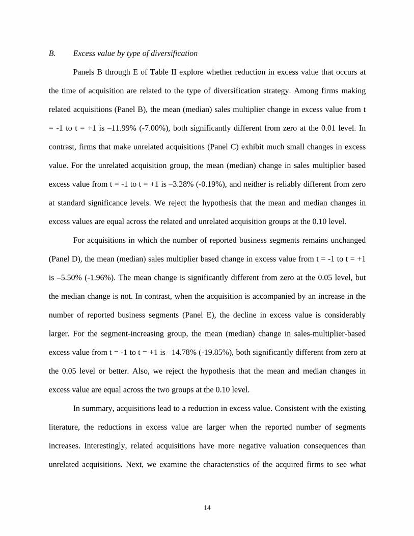
B. Excess value by type of diversification

Panels B through E of Table II explore whether reduction in excess value that occurs at

the time of acquisition are related to the type of diversification strategy. Among firms making

related acquisitions (Panel B), the mean (median) sales multiplier change in excess value from t

= -1 to t = +1 is –11.99% (-7.00%), both significantly different from zero at the 0.01 level. In

contrast, firms that make unrelated acquisitions (Panel C) exhibit much small changes in excess

value. For the unrelated acquisition group, the mean (median) change in sales multiplier based

excess value from t = -1 to t = +1 is –3.28% (-0.19%), and neither is reliably different from zero

at standard significance levels. We reject the hypothesis that the mean and median changes in

excess values are equal across the related and unrelated acquisition groups at the 0.10 level.

For acquisitions in which the number of reported business segments remains unchanged

(Panel D), the mean (median) sales multiplier based change in excess value from t = -1 to t = +1

is –5.50% (-1.96%). The mean change is significantly different from zero at the 0.05 level, but

the median change is not. In contrast, when the acquisition is accompanied by an increase in the

number of reported business segments (Panel E), the decline in excess value is considerably

larger. For the segment-increasing group, the mean (median) change in sales-multiplier-based

excess value from t = -1 to t = +1 is –14.78% (-19.85%), both significantly different from zero at

the 0.05 level or better. Also, we reject the hypothesis that the mean and median changes in

excess value are equal across the two groups at the 0.10 level.

In summary, acquisitions lead to a reduction in excess value. Consistent with the existing

literature, the reductions in excess value are larger when the reported number of segments

increases. Interestingly, related acquisitions have more negative valuation consequences than

unrelated acquisitions. Next, we examine the characteristics of the acquired firms to see what

15

role they play in explaining the decline in excess value for all acquirers and also for different

types of diversification.

C. Excess values of target firms

Table III presents excess values in the year prior to the acquisition (t = -1) for the target

firms in the M&A sample. For the full sample, based on sales multipliers, the mean (median)

excess value of the targets is –9.01% (-8.80%), both significantly less than zero at the 0.01 level.

The table also reports the relative size of the acquisition, calculated as the ratio of sales or assets

of the target to those of the acquirer at t = -1. The acquisitions are fairly large. The mean

(median) ratio of target sales to acquirer sales is 53.52% (24.41%). Given the low excess values

of the targets relative to those of the acquirers, it is natural to expect that the excess value of the

acquiring firms will decline as these poorly performing companies are merged into existing

operations, even if the acquisition itself does not destroy value.

Panels B through E report excess values and relative acquisition sizes for the various

subgroups. The most striking result is that the patterns in target firm excess values and relative

acquisition sizes closely parallel the declines in acquiring firm excess values documented in

Table II. Namely, target firms in related acquisitions are larger and more deeply discounted

relative to unrelated targets. In the related acquisition group (Panel B), the median sales

multiplier based excess value of the target firms is –13.05%, in comparison to a median excess

value of –3.25% in the unrelated acquisition group (Panel C). In addition, the relative size of the

median related acquisition (41.87%) is approximately three times larger than that of the median

unrelated acquisition (13.89%). Similar patterns are documented with respect segment-increasing

acquisitions. The median sales multiplier based excess value of target firms in the group with no

16

segment increases (Panel D) is –8.40%, in comparison to a median excess value of –18.51% for

targets in acquisitions that correspond to segment increases (Panel E). Additionally, the relative

sizes of the median acquisition in the no segment increase group is 23.4%, compared to a median

of 36.3% for the group with segment increases.

V. Explaining the apparent value loss in acquisitions

In this section, we determine the portion of the observed “value loss” that is attributable

to the acquisition of a unit with low excess value. Our strategy is straightforward. We compute

the excess value the combined firm would have if its parts were merged instantaneously at t = -1,

prior to the actual acquisition. This calculation estimates the excess value of the sum of the

combined firm’s parts, before the acquisition could have possibly destroyed any value.

More specifically, define P+1, the projected excess value at t = +1, as

,ln11

111

++

=−−

−−+ IVTIVA

MVTMVAP (1)

where MVA-1 and IVA-1 are the market value and imputed value of the acquirer at t = -1, and

MVT-1 and IVT-1 are for the target. The imputed values are calculated using the methodology of

Berger and Ofek (1995). This calculation determines the projected excess value of the combined

firm under the null hypothesis that the acquisition itself does not affect value. We compare the

projected excess value to the ex post excess value as determined by the Berger and Ofek

methodology.7

7 One data issue occurs in some unrelated acquisitions. When an unrelated acquisition does not result in a newbusiness segment being reported, the ex post excess value of the combined firm is based solely on the originalbusiness segments of the acquirer. The projected excess value, however, is based in part on an imputed excess valuefor the target linked to the target’s business segments, via IVT-1 in equation (1). For these observations, this issuemight introduce some noise into the ability of the projected excess value to predict ex post excess values.

17

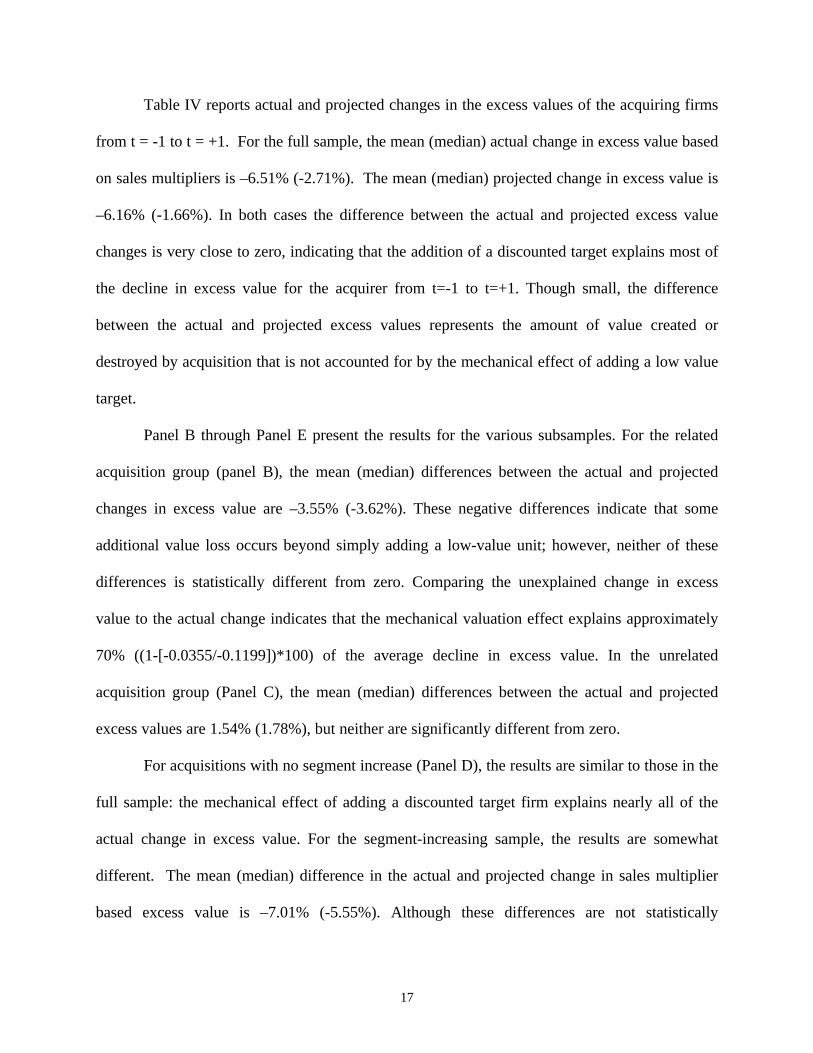
Table IV reports actual and projected changes in the excess values of the acquiring firms

from t = -1 to t = +1. For the full sample, the mean (median) actual change in excess value based

on sales multipliers is –6.51% (-2.71%). The mean (median) projected change in excess value is

–6.16% (-1.66%). In both cases the difference between the actual and projected excess value

changes is very close to zero, indicating that the addition of a discounted target explains most of

the decline in excess value for the acquirer from t=-1 to t=+1. Though small, the difference

between the actual and projected excess values represents the amount of value created or

destroyed by acquisition that is not accounted for by the mechanical effect of adding a low value

target.

Panel B through Panel E present the results for the various subsamples. For the related

acquisition group (panel B), the mean (median) differences between the actual and projected

changes in excess value are –3.55% (-3.62%). These negative differences indicate that some

additional value loss occurs beyond simply adding a low-value unit; however, neither of these

differences is statistically different from zero. Comparing the unexplained change in excess

value to the actual change indicates that the mechanical valuation effect explains approximately

70% ((1-[-0.0355/-0.1199])*100) of the average decline in excess value. In the unrelated

acquisition group (Panel C), the mean (median) differences between the actual and projected

excess values are 1.54% (1.78%), but neither are significantly different from zero.

For acquisitions with no segment increase (Panel D), the results are similar to those in the

full sample: the mechanical effect of adding a discounted target firm explains nearly all of the

actual change in excess value. For the segment-increasing sample, the results are somewhat

different. The mean (median) difference in the actual and projected change in sales multiplier

based excess value is –7.01% (-5.55%). Although these differences are not statistically

18

significant, they provide some evidence that segment-increasing acquisitions exhibit additional

value loss beyond that which can be explained by the characteristics of the target. In the case of

segment-increasing acquisitions, the mechanical valuation effect explains about 50% ((1-[-

0.0701/-0.1478])*100) of the average decline in the excess value of the acquirers.

To further explore how much of the observed value loss is attributable to a purely

mechanical effect of acquisition, Table V presents results from regressing the actual change in

excess value on the projected change in excess value. Statistical significance is based on White

(1980) standard errors. Using sales multipliers, the projected change in the value loss explains

20% of the variation in the actual change in value loss. This corresponds to a pairwise correlation

of 45% between the actual and predicted changes in value loss. Moreover, the estimated

regression coefficient on the projected value loss term is not statistically different from 1.0 (p-

value=0.847), indicating that the projected value loss is an unbiased predictor of the actual

change in excess value. The intercept in the regression is -0.0020, which is not significantly

different from zero (p-value=0.929). The intercept measures the unexplained portion of the

change in excess value and, given that it is nearly zero, indicates that essentially no additional

value loss remains after accounting for the characteristics of the acquired firm.

Table VI presents results from regressing the actual change in excess value on the

projected change in excess value and two indicator variables. In Panel A, the indicator is set

equal to one if the acquisition is related. Based on sales multipliers, the estimated coefficient on

the projected value loss is not significantly different from one (p-value = 0.946). The estimated

intercept is 0.0159 (p-value = 0.537), indicating that for unrelated acquisitions the characteristics

of the acquisition account for all of the observed change in excess values. For related

acquisitions, the coefficient estimate on the indicator variable is –0.0506, but is not significantly

19

different from zero (p-value=0.263). Though insignificant, the negative coefficient on the

indicator variable provides weak evidence that related acquisitions result in some additional

value loss that is not fully explained by the mechanical effect of adding a discounted target.

In Panel B, the indicator variable is set equal to one if the acquisition leads to a segment

increase. Consistent with the univariate results in Table IV, the coefficient on the indicator is –

0.0506, but is not significantly different from zero (two-sided p-value = 0.177). Comparing the

null that the number of segments does not matter to the alternative that increased number of

segments is bad, the coefficient is marginally significant (one-sided p-value = 0.088). The

negative coefficient on the indicator variable provides some evidence that segment-increasing

acquisitions result in additional value loss beyond that explained by the characteristics of the

target firm.

VI. Segment-increasing firms

Our M&A evidence shows that firms that are acquired tend to have significantly negative

excess values. By simply accounting for the valuations of the target firms, we explain most of the

negative valuation effects associated with mergers. However, only 31 of our acquisitions lead to

segment increases. Therefore, to more directly assess the applicability of our findings to the

literature that examines the valuation effects of diversification based on the number of business

segments, we examine a sample of firms that increase their number of business segments from

one to more than one.

A. Sample selection

20

From the set of all firms listed in the 1996 Compustat Industry Segment file, including

the research and historical files, we identify all firms that change from reporting one segment to

reporting multiple segments. We require that these firms have three years of data available,

centered on the date of segment increase, and that the firm report more than one segment in

periods t = 0 and t = +1. We concentrate on these firms, in part, because Lang and Stulz (1994)

show that the largest drop-off in q occurs between single-segment and two-segment firms. Our

initial sample consists of 359 firms from the period 1980 to 1995.

Firms increase their number of reported segments for a variety of reasons. Financial

Accounting and Standards Board (FASB) Statement 14 requires firms to report data for

individual lines of business that represent more than 10% of the firm’s total revenues, assets, or

profits. New segments may result from the acquisition of a new line of business, the internal

growth of an operation that finally passes one of these thresholds, or simple restructuring of

existing operations. Based on annual reports, 10-Ks and Investor Dealers' Digest Merger &

Acquisition reports from Lexis/Nexis, we group our sample firms into four categories related to

the reason for the increase in the number of reported business segments.

Under Generally Accepted Accounting Principles (APB 16, August 1970) firms are

required to discuss acquisitions in the footnotes of their filings. When the footnotes mention an

acquisition, we place the firm into one of several categories. If the acquired company operates

(does not operate) in an industry related to the existing operations of the diversifying firm, we

categorize the segment increase as a "related" ("unrelated") acquisition.8 For the related and

unrelated acquisitions, we attempt to establish at least a rough correspondence between the size

and industry of the increased segment (as listed on Compustat) and the acquired firm(s) (as

8We classify an acquisition as related if the SIC code for the target is in the same 4-digit SIC code as the acquirer.

21

identified from 10K footnotes and Lexis/Nexis). In 32 cases, either the size or industry of the

new segment does not match that for the acquired firm(s), which we categorize as "unclassified".

If we find no evidence of an acquisition in the footnotes, we include the segment increase

in the "no acquisition" group. Firms in this group may have added segments due to internal

growth, a decision to begin reporting a previously existing division, etc. Finally, since

Lexis/Nexis does not have reports for periods earlier than 1984, any firm diversifying before

1984 or otherwise missing the necessary statements or reports is categorized as "unclassified".

Table VII presents the distribution of the sample of diversifying firms by category. The

majority of segment increases result from acquisitions. Of the 235 (359 - 124) segment increases

that we can classify, 144 are related or unrelated acquisitions. These proportions are similar to

those in Hyland (1999), who reports that 150 out of 227 firms that increase from one segment to

more than one segment do so via acquisition. In our subsequent analysis, we focus primarily on

firms that expand via acquisition, but report selected data for other subsamples.

The primary difference between the M&A sample and the segment-increasing sample is

that in the former we only kept firms for which we could exactly identify the acquired unit.9 In

contrast, in the segment-increasing sample we do not require an exact match.10 Instead, we proxy

for the acquired unit by using the median single-segment firm among same-industry firms that

are removed from Compustat because they are acquired or involved in a merger, which is similar

9 The two other notable differences are that the segment-increasing sample only includes firms that start with asingle unit, and the segment-increasing sample contains some firms that increase their number of reported segments,even though they did not make an acquisition (the “no acquisition” group).10 A number of factors account for the difficulty in finding an exact match. In many cases, the segment increasesresult from partial acquisitions, acquisitions of private firms, or multiple acquisitions that occur over several years.For example, Tanknology acquired a private firm (Engineered Systems) in 1992. As another example, TPIEnterprises purchased approximately 20% of the movie theatre complexes operated by AMC Entertainment in 1989.In other cases, the reports or accounting statements do not provide specifics about the acquired firms. For example,in its 1993 Annual Report, Otter Tail Power reports that the "Health Services Operations" division "includes certainbusinesses purchased in 1993, including a diagnostic medical imaging company, a management company for anumber of diagnostic imaging companies, and a medical imaging company that sells and services diagnostic medicalimaging equipment and associated supplies and accessories".

22

to the benchmarking assumption made in other conglomeration analyses. Compustat footnote

code 35 indicates when firms on the annual industrial files are removed due to acquisition (code

01) or merger (code 04).

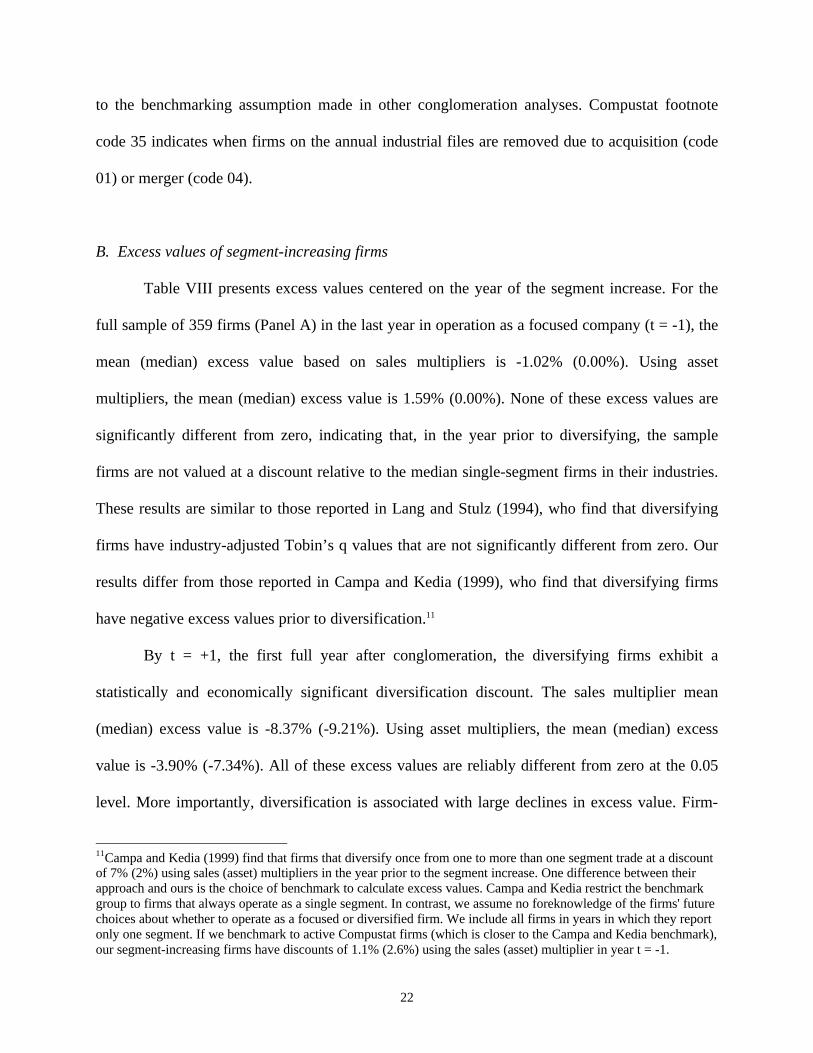
B. Excess values of segment-increasing firms

Table VIII presents excess values centered on the year of the segment increase. For the

full sample of 359 firms (Panel A) in the last year in operation as a focused company (t = -1), the

mean (median) excess value based on sales multipliers is -1.02% (0.00%). Using asset

multipliers, the mean (median) excess value is 1.59% (0.00%). None of these excess values are

significantly different from zero, indicating that, in the year prior to diversifying, the sample

firms are not valued at a discount relative to the median single-segment firms in their industries.

These results are similar to those reported in Lang and Stulz (1994), who find that diversifying

firms have industry-adjusted Tobin’s q values that are not significantly different from zero. Our

results differ from those reported in Campa and Kedia (1999), who find that diversifying firms

have negative excess values prior to diversification.11

By t = +1, the first full year after conglomeration, the diversifying firms exhibit a

statistically and economically significant diversification discount. The sales multiplier mean

(median) excess value is -8.37% (-9.21%). Using asset multipliers, the mean (median) excess

value is -3.90% (-7.34%). All of these excess values are reliably different from zero at the 0.05

level. More importantly, diversification is associated with large declines in excess value. Firm-

11Campa and Kedia (1999) find that firms that diversify once from one to more than one segment trade at a discountof 7% (2%) using sales (asset) multipliers in the year prior to the segment increase. One difference between theirapproach and ours is the choice of benchmark to calculate excess values. Campa and Kedia restrict the benchmarkgroup to firms that always operate as a single segment. In contrast, we assume no foreknowledge of the firms' futurechoices about whether to operate as a focused or diversified firm. We include all firms in years in which they reportonly one segment. If we benchmark to active Compustat firms (which is closer to the Campa and Kedia benchmark),our segment-increasing firms have discounts of 1.1% (2.6%) using the sales (asset) multiplier in year t = -1.

23

by-firm, the mean (median) change in excess value from t = -1 to t = +1 are -9.39% (-5.98%) and

-5.50% (-3.48%) based on sales and asset multipliers, respectively. In all cases the changes in

excess value are significant at the 0.01 level.

We now examine whether the change in excess value varies by the type of segment

increase. Note that much of the existing literature defines diversification based on the number of

reported segments. Given that we focus on changes in diversification, we therefore might expect

to observe a decline in excess value whenever a firm begins to report additional segments.

However, in some instances firms begin to report an increased number of segments because of

internal growth or a change in filing practice. In these “no acquisition” cases, the firm has not

changed substantially, even though the number of segments increased, so we do not expect to

find a significant decrease in excess value. In many cases, these firms have no significant change

in their scale or scope of operations because of the segment increase. They simply change their

reporting to include a new business segment. (For example, Cybex International reports a single

segment, "Medical and fitness eq.", in 1992. In 1993, Cybex operates two segments, "exercise

equipment" and "medical equipment". Total assets of the company increased only $5 million,

from $104 million in 1992 to $109 million in 1993.)

Panels B through D of Table VIII display excess values for firms grouped by category.

Consistent with our expectation, firms that diversify through internal growth have mean and

median excess values that are indistinguishable from zero prior to the increase in business

segments, and do not exhibit a significant change in excess value when the number of reported

business segments increases. The mean (median) sales multiplier based change in excess value

from t = -1 to t = +1 for the no acquisition group is -3.53% (0.00%), and neither is reliably

24

different from zero at standard significance levels. Therefore, there is no value loss from simply

operating in more than one segment because of internal growth or reporting change.

Firms that make unrelated acquisitions also have mean and median excess values that are

indistinguishable from zero prior to diversification, but exhibit large changes in excess value

after they increase the number of business segments. For the unrelated acquisition group, the

mean (median) change in sales-based excess value from t = -1 to t = +1 is -13.69% (-8.06%),

both significantly less than zero at the 0.01 level. Somewhat surprisingly, firms making related

acquisitions have the largest decline in excess value. The related acquisition group has positive

excess values in year t = -1, and large negative excess values in year t = +1. The mean (median)

change in sales-based excess value from t = -1 to t = +1 is -30.05% (-26.02%), and both are

significantly less than zero at the 0.01 level (However, the related acquisition group has only 18

observations, so these numbers should be treated cautiously). This finding is similar to our

results for the M&A sample, where we also found that related acquisitions were associated with

larger declines in excess values. Recall for the M&A case that we traced those large drops in

excess value to the acquisition of a large discounted unit.

We statistically reject the hypothesis that the mean and median changes in excess value in

Panels B through D are equal across the three groups at the 0.05 level. In pairwise comparisons

based on sales multipliers, the mean changes in excess value are not equal for the no acquisition

and unrelated acquisition groups at the 0.10 level. The differences in the medians are not

significant. The differences in the mean (median) changes in excess values across the no

acquisition and related acquisition subsamples are significant at the 0.05 (0.01) level. The

differences in the mean changes in excess values across the related and unrelated groups are not

significant, but the differences in the medians are significant at the 0.05 level.

25

C. Excess values of acquired firms

We now examine the characteristics of firms that are acquired to see what role they play

in the conglomerate discount of segment-increasing firms. Table IX presents excess values for

the acquired firms over the period leading up the time they are removed from Compustat. Two

key points stand out. First, the excess values are significantly below zero in year t = -1, just prior

to when the firm is acquired. Second, there is a notable downward trend in the years leading up

to the firm's acquisition.12 For example, the mean excess values based on sales multipliers are

-5.90% in year t = -3, -11.31% in year t = -2, and -15.53% in year t = -1, the year prior to

removal. These excess values are all significantly different from zero at the 0.01 level. Similar,

but less dramatic patterns appear using asset multipliers. With discounts of this magnitude, it is

natural to expect that the excess value of segment-increasing firms will decline as poorly

performing companies are merged into existing operations, even if diversification itself does not

destroy value.

VII. Explaining (part of) the apparent value loss in segment-increasing firms

For our sample, segment-increasing firms (i.e., the parents) have excess value of zero

prior to the segment increase and acquired firms in the population are heavily discounted prior to

acquisition. To determine the portion of the ex post discount that is observed in segment-

increasing firms that is attributable to the acquisition of a unit with negative excess value, we

follow the same strategy we used in the acquisition sample. We project the excess value the

conglomerate would have if its parts were merged instantaneously at t = -1, prior to the actual

12 This is similar to results in Lang, Stulz and Walkling (1989), who find that the q ratios of target firms in tenderoffers decline significantly over the five years preceding the tender offer.

26

segment increase. The only difference is that for the sample of segment-increasing firms we

calculate the imputed value of the new segment(s) using the median excess value from the

population of acquired firms in the same industry as segment i (based on the tightest SIC group

with at least 5 observations) measured at t = -1. This calculation determines the excess value of

the conglomerate under the null hypothesis that the act of diversification itself does not affect

value.

We only perform this calculation for the unrelated acquisition group. The comparison is

not feasible for the firms making related acquisitions because the original parent division of these

firms is often dissolved in conjunction with the increase in the number of reported business

segments. Specifically, of the 18 firms making related acquisitions, the segment ID of the

original parent at t = -1 continues to exist at t = +1 for only six firms.

To examine how much of the actual value loss is attributable to a purely mechanical

outcome from the acquisition, Table X presents results from regressing the actual change in

excess value on the projected change in excess value. Using sales multipliers, the projected

change in the value loss explains 18% of the variation in the actual change in value loss. This

corresponds to a pairwise correlation of 42% between the actual and predicted changes in value

loss. Moreover, the estimated regression coefficient on the projected value loss term is not

statistically different from one (p-value=0.631), indicating that the projected value loss estimates

do a good job at capturing the cross-sectional variation in the actual changes in excess values.

The intercept in the regression is -0.0655, which is significantly different from zero at the 0.10

level. The negative intercept indicates that the unexplained portion of the change in excess value

is approximately -6.6%, indicating that the acquisition of a poorly performing unit explains about

one-half of the total change in excess value of -13.7%.

27

We repeat the regression analysis using asset multipliers. In this case, the intercept of

-5.66% indicates that the purchase of a poorly performing unit explains about two-fifths of the

total change in excess value of -9.57%. Recall that the choice of accounting method can lead to

problems when calculating excess values using asset multipliers. Plumlee and Wolf (2000)

provide evidence that if we could adjust for the effect of purchase accounting in combination

with the addition of a poorly performing unit, the projected value based on asset multipliers

would explain more than two-fifths of the diversification discount in conglomerates.

Finally, note that we would rather base all of our projected values on "the value that the

new unit would have had at t = +1, had it continued to operate as a single-segment firm." If the

downward trend in excess values shown in Table IX would have continued through t = +1, the

portion of excess value explained by mechanically adding up the parts of the conglomerate

would be even larger.

VIII. Conclusions

During the 1990s academic research and popular press reports generally indicated that

corporate diversification was bad. By some accounts, conglomerate firms were discounted by as

much as 15% from the value that could be attained by simply breaking them up and operating the

divisions as stand-alone companies.

Our main insight is related to how the value-loss due to conglomeration is usually

calculated: by valuing each division of a conglomerate as a multiple of the value of the median

stand-alone firm in its same industry. We show that the firms that are acquired in diversifying

acquisitions, as well as the sample of firms that are removed from Compustat due to merger or

acquisition, are priced at a discount (relative to the median stand-alone firm in the same industry)

28

prior to becoming part of a conglomerate. When this discounted unit is added to an existing firm,

not surprisingly, it has a negative effect on the excess value of the combined businesses. We

demonstrate that accounting for this pre-acquisition discount in acquired units accounts for half

or more of the ex post discount in the combined firm. The implication is that if corporate

diversification destroys value in our sample, it only destroys a fraction of what the common

valuation techniques imply. To the extent that our results carry over to the full sample of

conglomerate firms, they imply that comparing the divisions of conglomerates to median stand-

alone firms can overstate the discount of diversified firms.

For our sample, with one exception, excess value is reduced for all types of acquisitions:

related or unrelated; segment-increasing or not. The most important factor driving the extent of

excess value reduction in all of these subgroups is how large and how heavily discounted the

acquired unit is, implying that our insight plays an important role in the valuation of

conglomerate firms. The one exception is that excess value is not reduced when a firm increases

its number of business segments due to a pure reporting change.

We do not claim to have explained away the entire diversification discount, nor do we

claim that conglomeration is not bad in some cases. Based on positive market reactions to the

breakup of some firms (Berger and Ofek (1996)), it seems clear that corporate diversification is

bad in for some firms. The implications from our analysis are that 1) care needs to be taken when

benchmarking the value of conglomerate divisions and that 2) the magnitude of the

diversification discount might be smaller, and apply to less firms, than is commonly believed.

29

Appendix

The Purchase method of merger accounting and excess value

To understand how asset multipliers might be affected by accounting choice at the time

of segment increase, we return to the example in Table I.

[INSERT TABLE AI HERE.]

The main difference from the earlier example is that is this example, under the purchase method,

the assets of firm T are marked up to market value (70) at the time of purchase. This increases

the total book value of assets to 185 instead of 180.

As we calculate the excess value for the combined firm, the imputed value of the old

segment to be the same as in the earlier example. However, the imputed value of the newly

acquired division is based upon its new book value of assets. The new imputed value is 6.25

higher than it would be without purchase accounting ( (70-65)*1.25 ). The higher imputed value

results in a lower excess value (ln[185/202.5] = -0.09 instead of ln[185/196.25] = -0.06).

An implicit assumption in using the asset multipliers to calculate excess value is that

assets are accounted for similarly by diversified and focused firms. Therefore, this difference in

the actual accounting method serves to increase the magnitude of both the unexplained and total

change in excess value when using asset multipliers. Plumlee and Wolf (2000) investigate in

detail the effect of the method of accounting on multiple-based valuation techniques. Based on

their conclusions, we deemphasize asset-based multiple valuation in our paper.

30

References

Amihud, Yakov and Baruch Lev, 1981, "Risk reduction as a managerial motive for conglomeratemergers", Bell Journal of Economics, 12, 605-617.

Anderson, Ronald, Thomas Bates, John Bizjak and Michael Lemmon, 1999, "Corporategovernance and firm diversification", Financial Management, forthcoming.

Berger, Philip G. and Eli Ofek, 1995, "Diversification's effect on firm value", Journal ofFinancial Economics, 37, 39 - 65.

Berger, Philip G. and Eli Ofek, 1996, "Bustup takeovers of value destroying diversified firms",Journal of Finance, 51, 1175-1200.

Berger, Philip G. and Eli Ofek, 1999, "Causes and effects of corporate diversification programs",Review of Financial Studies, 12, 311-345.

Billet, Matthew, and David Mauer, 1998, "Cross-subsidies, external financing constraints, andthe contribution of internal capital markets to firm value", Working paper, University of Iowa.

Brown, Stephen, and Jerold Warner, 1980, "Measuring security price performance", Journal ofFinancial Economics, 8, 205-258.

Campa, Jose and Simi Kedia, 1999, "Explaining the diversification discount", Working Paper,Harvard Business School.

Chevalier, Judith, 1999, "Why do firms undertake diversifying mergers? an investigation of theinvestment policies of merging firms", Working Paper, University of Chicago.

Comment, Robert and Gregg A. Jarrell, 1995, "Corporate focus and stock returns", Journal ofFinancial Economics, 37, 67-87.

Denis, David J., Diane K. Denis and Atulya Sarin, 1997, "Agency problems, equity ownership,and corporate diversification", Journal of Finance, 52, 135-160.

Hubbard, R. Glenn and Darius Palia, 1999, "A reexamination of the conglomerate merger wavein the 1960s: an internal capital markets view", Journal of Finance, 54, 1131-1152.

Hyland, David, 1999, "Why firms diversify: an empirical examination", Working Paper,University of Texas Arlington.

Jensen, M.C., 1986, "Agency costs of free cash flow, corporate finance, and takeovers",American Economic Review, 76, 323-329.

John, Kose and Eli Ofek, 1995, "Asset sales and increase in focus", Journal of FinancialEconomics, 37, 105-126.

31

Khorana, Ajay and Marc Zenner, 1998, "Executive compensation of large acquirers in the1980s", Journal of Corporate Finance, 4, 209-240.

Lamont, Owen, 1997, "Cash flow and investment: evidence from internal capital markets",Journal of Finance, 52, 83-110.

Lamont, Owen, and Christopher Polk, 1999, "The diversification discount: cash flows vs.returns", Working paper, University of Chicago.

Lang, Larry, René Stulz, and Ralph Walkling, 1989, "Managerial performance, Tobin's q, andthe gains from successful tender offers", Journal of Financial Economics, 24, 137-154.

Lang, Larry and René Stulz, 1994, "Tobin's q, corporate diversification and firm performance",Journal of Political Economy, 102, 1248-1280.

Lewellen, Wilbur, 1971, "A pure financial rationale for the conglomerate merger", Journal ofFinance, 26, 521-537.

Lins, Karl and Henri Servaes, 1999, "International evidence on the value of corporatediversification", Journal of Finance, forthcoming.

Loughran, Tim and Anand Vijh, 1998, "Do long-term shareholders benefit from corporateacquisitions?", Journal of Finance, 52, 1765-1790.

Maksimovic, Vojislav and Gordon Phillips, 1998, "Optimal firm size and the growth ofconglomerates and single industry firms", Working Paper, University of Maryland.

Matsusaka, John G. and Vikram Nanda, 1994, "A theory of the diversified firm, refocusing anddivestiture", Working paper, University of Southern California.

May, Don O., 1995, "Do managerial motives influence firm risk reduction strategies?", Journalof Finance, 50, 1291-1308.

Piotroski, Joseph, 1999, "The impact of newly reported segment information on marketexpectations and stock prices", Working Paper, University of Michigan.

Plumlee, Marlene and Jack Wolf, 2000, “Purchase or pooling? The Impact of Accounting Choiceon the Calculation of Excess Value”, Working Paper, University of Utah.

Rajan, Raghuram, Henri Servaes and Luigi Zingales, 1999, "The cost of diversity: thediversification discount and inefficient investment", Journal of Finance, forthcoming.

Roll, Richard, 1986, "The hubris hypothesis of corporate takeovers", Journal of Business, 59,197-216.

32

Scharfstein, David, and Jeremy Stein 1997, "The dark side of internal capital markets: divisionalrent seeking and inefficient investment", Working Paper, Massachusetts Institute of Technology.

Scharfstein, David, 1998, "The dark side of internal capital markets II: evidence from diversifiedconglomerates", Working Paper, Massachusetts Institute of Technology.

Servaes, Henri, 1996, "The value of diversification during the conglomerate merger wave",Journal of Finance, 51, 1201-1225.

Shin, Hyun-Han, and René Stulz, 1997, "Are internal capital markets efficient?", The QuarterlyJournal of Economics, 531-552.

Stein, Jeremy, 1997, "Internal capital markets and the competition for corporate resources",Journal of Finance, 52, 111-133.

Stulz, René M., 1990, "Managerial discretion and optimal financial policies", Journal ofFinancial Economics, 26, 3-27.

Weston, J. Fred, 1970, "Diversification and merger trends", Business Economics, 5, 50-57.

33

Table IExample of Negative Excess Value with No Real Value Destruction

This table shows how acquiring target Firm T could affect Firm A's excess value. By construction, total marketvalue is conserved so no market value is destroyed. The benchmark represents the median market/sales ratio ofsingle-segment same-industry firms.

Firm A Firm T CombinationSales a 100.00 65.00 165.00Market Value 115.00 70.00 185.00Benchmark Market/Sales Ratio 1.15 1.25Imputed Value 115.00 81.25 196.25

Excess Value 0.000 -0.15 b -0.06 c

a This could be book value of assets if an asset multiplier is used.b Excess value is calculated as ln[70/(65*1.25)] = ln[70/81.25] = ln[0.862] = -0.15.c Excess value is calculated as ln[(115+70)/(100*1.15 + 65*1.25)]=ln[185/196.25]=ln[0.943]=-0.06.

34

Table IIExcess Values for Acquirors

This table reports excess values for the year prior to and the year following the acquisition. The sample consists of286 firms that completed acquisitions between 1980 and 1995 with sufficient data to calculate excess values as asdefined in Berger and Ofek (1995). Panel A reports results for the full sample while Panels B through E examinesubsamples.

Sales Multiplier Asset MultiplierPeriod Mean Median Mean Median

Panel A: Full Sample (286 firms)-1 0.1547 *** 0.1470 *** 0.1104 *** 0.0541 ***+1 0.0897 *** 0.0927 *** 0.0506 ** -0.0127

Change (t=-1 to t=+1) -0.0651 *** -0.0271 ** -0.0597 *** -0.0529 ***

Panel B: Related Acquisition ( 106 firms)-1 0.1982 *** 0.1389 *** 0.1161 *** 0.0652 ***+1 -0.0783 ** 0.0496 * 0.0060 -0.0254

Change (t=-1 to t=+1) -0.1199 *** -0.0700 *** -0.1102 *** -0.1030 ***

Panel C: Unrelated Acquisition (180 firms)-1 0.1292 *** 0.1470 *** 0.1070 *** 0.0445 ***+1 0.0964 *** 0.1027 *** 0.0770 *** 0.0000 *

Change (t=-1 to t=+1) -0.0328 -0.0019 -0.0301 -0.0035

Panel D: No Segment Increase (255 firms)-1 0.1657 *** 0.1693 *** 0.1159 *** 0.0573 ***+1 0.1107 *** 0.1170 *** 0.0601 *** -0.0026

Change (t=-1 to t=+1) -0.0550 ** -0.0196 -0.0558 *** -0.0553 ***

Panel E: Segment Increase (31 firms)-1 0.0643 0.1140 0.0648 0.0000+1 -0.0835 -0.1073 -0.0273 -0.0482

Change (t=-1 to t=+1) -0.1478 *** -0.1985 ** -0.0921 -0.0225

*, **, and ***, significantly different from zero at the 10, 5 and 1 percent levels, respectively.

35

Table IIIExcess Values for Targets

This table reports excess values of target firms in the year prior to being acquired. The sample consists of 286 firmsthat were acquired between 1980 and 1995 with sufficient data to calculate excess values as as defined in Berger andOfek (1995). Panel A reports results for the full sample while Panels B through E examine subsamples.


Panel A: Full Sample (286 firms)-1 -0.0901 *** -0.0880 *** 0.0019 -0.0255

Relative size 0.5352 0.2441 0.4518 0.1962

Panel B: Related Acquisition ( 106 firms)-1 -0.1715*** -0.1305 *** -0.0524 * -0.0530 *

Relative size 0.7263 0.4187 0.5962 0.3354

Panel C: Unrelated Acquisition (180 firms)-1 -0.0422 -0.0325 0.0339 -0.0032

Relative size 0.4227 0.1389 0.3668 0.1383

Panel D: No Segment Increase (255 firms)-1 -0.0766 ** -0.0840 *** 0.0011 *** -0.0260 ***

Relative size 0.5293 0.2343 0.4563 *** 0.1874

Panel E: Segment Increase (31 firms)-1 -0.2013 ** -0.1851 * 0.0089 0.0000

Relative size 0.5839 0.3630 0.4149 0.2364


36

Table IVActual and Projected Changes in Excess Values for Acquirors

This table reports excess values for the year prior to and the year following the acquisition. The sample consists of286 firms that completed acquisitions between 1980 and 1995 with sufficient data to calculate excess values asdefined in Berger and Ofek (1995). Panel A reports results for the full sample while Panels B through E examinesubsamples.


Panel A: Full Sample (286 firms)Actual Change -0.0651 *** -0.0271 ** -0.0597 *** -0.0529 ***Projected Change -0.0616 *** -0.0166 *** -0.0367 *** -0.0086 ***

Difference -0.0035 0.0032 -0.0231 -0.0142

Panel B: Related Acquisition (180 firms)Actual Change -0.1199 *** -0.0700 *** -0.1102 *** -0.1030 ***Projected Change -0.0844 *** -0.0419 *** -0.0514 *** -0.0150 ***

Difference -0.0355 -0.0362 -0.0588 ** -0.0772 **,a

Panel C: Unrelated Acquisition (106 firms)Actual Change -0.0328 -0.0019 -0.0301 -0.0035Projected Change -0.0482 *** -0.0088 *** -0.0280 *** -0.0052 ***

Difference 0.0154 0.0178 -0.0021 0.0127

Panel D: No Segment Increase (255 firms)Actual Change -0.0550 ** -0.0196 -0.0558 *** -0.0109 ***Projected Change -0.0597 *** -0.0166 *** -0.0383 *** -0.0553 ***

Difference 0.0046 0.0153 -0.0175 -0.0167

Panel E: Segment Increase (31 firms)Actual Change -0.1478 *** -0.1985 ** -0.0921 -0.0225Projected Change -0.0776 ** -0.0158 * -0.0227 -0.0030

Difference -0.0701 -0.0555 -0.0694 -0.0026

*, **, and ***, significantly different from zero at the 10, 5 and 1 percent levels, respectively.a The differences between the actual and projected changes in excess value for the related and unrelated subsamplesare statistically different at the 5% level.

37

( ) ( )1111 −+−+ −+=− APAA βα

( ) ( ) ( )•+−+=− −+−+ I 1111 λβα APAA

Table VRelationship Between Projected and Actual Excess Values

This table reports regression results examining how well the projected excess values actually predict the ex postexcess value. The regression model is

where A+1 is the actual ex post excess value, P+1 is the projected ex post excess value and A-1 is the ex ante excessvalue. Standard errors are presented in parentheses. P-values for the null hypotheses that α=0 and β=1 are reportedin brackets.

Coefficient onProjected Change

Adj. R2 Intercept (P+1 – A-1)

Actual Change in 0.1995 -0.0020 1.0234Sales Multiplier (0.0228) (0.1206)(A+1-A-1) [0.9216] [0.8742]

Actual Change in 0.1259 -0.0259 0.9241Asset Multiplier (0.0186) (0.1425)(A+1-A-1) [0.1434] [0.6379]

Table VIRelationship Between Projected and Actual Excess Values

This table reports regression results examining how well the projected excess values actually predict the ex postexcess value. The regression models are

where A+1 is the actual ex post excess value, P+1 is the projected ex post excess value, A-1 is the ex ante excess valueand I(·) is an indicator variable for relatedness or segment increase. Standard errors are presented in parentheses. P-values for the null hypotheses that α=0 and β=1 and λ=0 are reported in brackets.

Coefficient on Coefficient onProjected Change Indicator Variable

Adj. R2 Intercept (P+1 – A-1) I(·)Panel A: Relatedness Indicator

Actual Change in 0.2003 0.0159 1.0010 -0.0506Sales Multiplier (0.0277) (0.1211) (0.0448)(A+1-A-1) [0.5371] [0.9462] [0.2631]

Actual Change in 0.1306 -0.0048 0.9036 -0.0590Asset Multiplier (0.0228) (0.1427) (0.0371)(A+1-A-1) [0.8360] [0.5392] [0.1011]

Panel B: Segment Increase Indicator

Actual Change in 0.1999 0.0058 1.0193 -0.0745Sales Multiplier (0.0239) (0.1206) (0.0692)(A+1-A-1) [0.7933] [0.8973] [0.1767]

Actual Change in 0.1252 -0.0202 0.9290 -0.0508Asset Multiplier (0.0197) (0.1427) (0.0576)(A+1-A-1) [0.2804] [0.6662] [0.4178]

38

Table VIIDistribution of Diversification Sample by Acquisition Classification

The table reports the number of segment increasing firms in the various acquisition categories. The no acquisitiongroup contains firms for which the segment increase results from either internal growth or a reporting change. Theunrelated acquisition group contains firms for which the segment increase results from acquisitions that areunrelated to the firm’s original industry. The related acquisition group contains firms for which the segment increaseresults from acquisitions related to the firms original industry. The related and unrelated classifications areperformed at the 3-digit SIC code level. The unclassified group includes firms whose segment increase occurredbefore 1984, the earliest that financial statements are available on Lexis-Nexis Academic Universe, are foreigncompanies with different accounting standards or are businesses for which we cannot identify the source of thesegment increase. The sample consists of 359 firms that begin reporting multiple business segments over the period1980-1994, and that have three years of financial data centered on the year of the segment increase.

FirmsNo acquisition 91Unrelated acquisitions 126Related acquisitions 18Unclassified 124

Total 359

39

Table VIIIExcess Values for Firms that Increase the Number of Reported Segments

This table reports excess values for the year prior to and the year following the first year in which more than onesegment is reported. The sample consists of 359 firms that changed from reporting one segment at year t = -1 toreporting more than one segment during years t = 0 and t = +1. Excess values are calculated as defined in Berger andOfek (1995) and are winsorized at ±1.386. Paired differences are the firm-specific differences from period t = -1 toperiod t = +1. Panel A reports results for the full sample while Panels B through D examine subsamples.


Panel A: Full Sample (359 firms)-1 -0.0102 0.0000 0.0159 0.0000+1 -0.0837 *** -0.0921 *** -0.0390 ** -0.0734 ***

Change (t=-1 to t=+1) -0.0939 *** -0.0598 *** -0.0550 *** -0.0348 ***

Panel B: No Acquisition Group (91 firms)-1 0.0147 0.0000 -0.0162 0.0000+1 -0.0206 -0.0125 -0.0291 -0.0664

Change (t=-1 to t=+1) -0.0353 0.0000 -0.0129 0.0000

Panel C: Unrelated Acquisition Group (126 firms)-1 0.0123 0.0000 0.0368 -0.0080+1 -0.1246 *** -0.1010 *** -0.0589 * -0.0874 **

Change (t=-1 to t=+1) -0.1369 *** -0.0806 *** -0.0956 *** -0.0416 **

Panel D: Related Acquisition Group (18 firms)-1 0.1793 * 0.0946 0.1725 * 0.0345+1 -0.1212 -0.1189 -0.0039 -0.0254

Change (t=-1 to t=+1) -0.3005 *** -0.2602 *** -0.1765 *** -0.1245 ***


Table IXExcess Values for Single-Segment Firms that are Merged or Acquired

This table reports excess values for the three years before the firm was removed from Compustat due to merger oracquisition. The sample consists of 712 firms. Excess values are calculated as defined in Berger and Ofek (1995)except that values are winsorized at ±1.386 instead of being truncated at those values.


-3 -0.0590 *** -0.0532 *** 0.0075 -0.0047-2 -0.1131 *** -0.1045 *** -0.0352 *** -0.0334 ***-1 -0.1553 *** -0.1517 *** -0.0443 -0.0457 ***


40

( ) ( )1111 −+−+ −+=− APAA βα

Table XRelationship Between Projected and Actual Excess Values

This table reports regression results examining how well the projected excess values actually predict the ex postexcess value. The regression model is

where A+1 is the actual ex post excess value, P+1 is the projected ex post excess value and A-1 is the ex ante excessvalue. All excess values are winsorized at ±1.386. Standard errors are presented in parentheses. P-values for the nullhypotheses that α=0 and β=1 are reported in brackets.

Coefficient onProjected Change

Adj. R2 Intercept (P+1 – A-1)

Actual Change in 0.1800 -0.0655 1.1017Sales Multiplier (0.0351) (0.2115)(A+1-A-1) [0.0647] [0.6314]

Actual Change in 0.1517 -0.0566 0.8210Asset Multiplier (0.0254) (0.1739)(A+1-A-1) [0.0276] [0.3053]

41

Table AIExample of Greater Negative Excess Value Under Purchase Method

This table shows how the acquisition of Firm T could affect Firm A’s excess value. The example illustrated in thistable is similar to that in Table I and is intended to highlight the effect of the purchase method of accounting foracquisitions. Under the purchase method, the book value of assets of the acquired division is marked up to thepurchase price rather than remaining at the historical cost of the assets. By construction, total market value isconserved so no market value is destroyed. Under the purchase method of accounting for an acquisition, the bookvalue of assets of the acquired unit is marked up to market value at the date of acquisition. We assume that theacquiring firm pays no premium for the acquired business. The benchmark is the median market/assets ratio of thetightest matched SIC group with at least 5 observations.

Firm A Firm T CombinationAssets 100.00 65.00 170.00 a

Market Value 115.00 70.00 185.00Benchmark Market/Assets ratio 1.15 1.25

Excess Value -0.000 -0.15 b -0.09 c

a Book value of assets of the combined firm is found by adding the book value of the existing division and themarket value of the newly acquired division.

b Excess value is calculated as ln[70/(65*1.25)] = ln[70/81.25] = ln[0.862] = -0.15.c Excess value is calculated as ln[(115+70)/(100*1.15 + 70*1.25)]=ln[185/202.5]=ln[0.914]= -0.09.

Does Corporate Diversification Destroy Value?

Documents

Transcript of Does Corporate Diversification Destroy Value?