February 20, 2007 To: AISI Committee Members Subject: Progress Report No. 3

Direct Strength Design for Cold-Formed Steel Members with Perforations Please find enclosed the third progress report summarizing our research efforts to extend the Direct Strength Method to cold-formed steel members with perforations. Our focus during this research period was on laboratory tests of columns with holes and the elastic buckling of cold-formed steel beams with holes. The column experiments revealed a tangible connection between elastic buckling and load-deformation response. The elastic buckling study uncovered unique elastic buckling modes reminiscent of those observed in compression members with holes. The completed body of work for this project is now revealing key trends which will allow us to navigate the research ahead with added confidence and clarity. Sincerely,

Cris Moen moen@jhu.edu

Ben Schafer schafer@jhu.edu

Summary of Progress The primary goal of this AISI-funded research is to extend the Direct Strength Method to cold-formed steel members with holes. Research begins September 2005 Progress Report #1 February 2006 Accomplishments:

• Evaluated the ABAQUS S9R5, S4, and S4R thin shell elements for accuracy and versatility in thin-walled modeling problems

• Studied the influence of element aspect ratio and element quantity when modeling rounded corners in ABAQUS

• Developed custom MATLAB tools for meshing holes, plates, and cold-formed steel members in ABAQUS

• Determined the influence of a slotted hole on the elastic buckling of a structural stud channel and classified local, distortional, and global buckling modes

• Investigated the influence of hole size on the elastic buckling of a structural stud channel

• Performed a preliminary comparison of existing experimental data on cold-formed steel columns with holes to DSM predictions

• Conducted a study on the influence of the hole width to plate width ratio on the elastic buckling behavior of a simply supported rectangular plate

Papers from this research: Moen, C., Schafer, B.W. (2006) “Impact of Holes on the Elastic Buckling of Cold-Formed Steel Columns with Application to the Direct Strength Method”, Eighteenth International Specialty Conference on Cold-Formed Steel Structures, Orlando, FL. Moen, C., Schafer, B.W. (2006) “Stability of Cold-Formed Steel Columns With Holes”, Stability and Ductility of Steel Structures Conference, Lisbon, Portugal.

Summary of Progress (continued) Progress Report #2 August 2006 Accomplishments:

• Evaluated the influence of slotted hole spacing on the elastic buckling of plates (with implications for structural studs)

• Determined the impact of flange holes on the elastic buckling of an SSMA structural stud

• Conducted a preliminary investigation into the nonlinear solution algorithms available in ABAQUS

• Compared the ultimate strength and load-displacement response of a rectangular plate and an SSMA structural stud column with and without a slotted hole using nonlinear finite element models in ABAQUS

• Calculated the effective width of a rectangular plate with and without a slotted hole using nonlinear finite element models in ABAQUS

Progress Report #3 February 2007 Accomplishments:

• Conducted an experimental study to evaluate the influence of a slotted web holes on the compressive strength, ductility, and failure modes of short and intermediate length Cee channel columns

• Studied the influence of slotted web holes on the elastic buckling behavior of cold-formed steel Cee channel beams and identified unique hole modes similar to those observed in compression members

• Demonstrated that the Direct Strength Method is a viable predictor of ultimate strength for beams with holes

1

1 Introduction

The research work presented in this progress report represents a continuing

effort to develop a general design philosophy that relates elastic buckling

behavior to the ultimate strength of cold-formed steel members with

perforations. The general framework for this philosophy is being developed

around the Direct Strength Method (DSM), which uses the local, distortional, and

global elastic buckling modes to predict the ultimate strength of cold-formed

steel members (NAS 2004, Appendix 1).

The final objective of this research project is to extend DSM to cold-formed

steel columns and beams with holes, which will be met through research goals

defined in three phases:

Phase I

1. Study the influence of holes on the elastic buckling of cold-formed

steel members.

2. Formalize the identification of buckling modes for members with

holes.

3. Compare existing experimental data on members with holes to the

current DSM specification.

2

Phase II

1. Increase our understanding of post-buckling mechanisms for members

with holes through non-linear finite element models and laboratory

testing

2. Formalize the relationship between elastic buckling and ultimate

strength for members with holes

Phase III

1. Modify the current DSM specification to account for members with

holes

2. Experimentally validate DSM as a rational analysis method for any

cold-formed member with holes

3. Develop open-source tools that engineers may use for easy application

of DSM to members with holes

Research summarized in Progress Report #1 addressed the Phase I goals for

cold-formed steel compression members with elastic buckling studies that

evaluated the influence of holes on thin plates and cold-formed steel channel

studs. Progress Report #2 continued the elastic buckling research by studying

the influence of flange holes in SSMA structural studs and the impact of slotted

web hole spacing on the performance of an SSMA structural stud. The report

also presented preliminary nonlinear finite element model results of thin plates

and cold-formed steel compression members with holes.

3

This document, Progress Report #3, summarizes both ultimate strength and

elastic buckling studies that address all three phases of this research program.

An experimental study of 24 column specimens is conducted to evaluate the

influence of slotted web holes on the compressive strength and failure modes of

short and intermediate length columns. The laboratory tests serve three

purposes: (1) to provide direct observations of the failure progression of thin-

walled compression members, (2) to add to the existing body of experimental

data on cold-formed steel columns with holes, and (3) to obtain load-

displacement responses of cold-formed steel specimens for the calibration of

future nonlinear finite element models.

An elastic buckling study on the influence of holes in beams is also

presented in this report. The elastic buckling modes of 72 beam specimens

(associated with existing experimental data) are calculated with eigenbuckling

analyses. A similar study for compression members with holes is summarized in

Progress Report #1 (Moen and Schafer 2006). Unique hole modes created by the

presence of slotted web holes are identified and classified. These buckling

modes are then used in combination with pure local (L), distortional (D), and

global (G) elastic buckling modes to calculate flexural strength predictions with

the Direct Strength Method. Conclusions are drawn regarding the viability of

DSM as a predictor of flexural strength and connections between the unique

holes modes of flexural and compression members are discussed.

4

2 Laboratory Investigation of Cold-Formed Steel Columns with Holes

2.1 Acknowledgements The cold-formed steel column tests described in this section were

completed with a team effort from the individuals below:

Eric Harden Latrobe Hall Machine Shop Walter Krug Maryland Hall Machine Shop Michael Franckowiak Maryland Hall Machine Shop Dr. Rachel Sangree Johns Hopkins Postdoctoral Researcher Jack Spangler Senior Mechanical Engineer – Structures Lab Nickolay Logvinosky Structures Lab Technician Mario Fasano Johns Hopkins Senior Rebecca Pierce Johns Hopkins Freshman Dawneshia Sanders Baltimore Polytechnic Institute Senior Alexander Pei High School Intern

Also, thank you to Clark Western for supplying the structural studs tested in this

study.

2.2 Introduction

Observing the behavior of cold-formed steel columns under load provides a

unique perspective on the failure of a column. Because a cold-formed steel

column is a thin-walled member, buckling emerges early in the load response.

The local and distortional buckling modes appear before your eyes, and the step-

by-step progression to failure can be visualized and digested. In this study, 24

cold-formed steel lipped Cee channel columns with and without slotted web

5

holes are tested to failure. The influence of holes on column ultimate strength

and failure modes are discussed. The elastic buckling behavior for each

specimen is determined and the tested data is then compared to DSM

predictions.

2.3 Experimental Program

2.3.1 Column Specimen Parameters

The column dimensions are chosen to ensure that elastic buckling modes

will influence the column ultimate strengths. Steel Stud Manufacturers

Association (SSMA) 362S162-33 and SSMA 600S162-33 structural stud cross

sections are considered in this study. The nominal steel sheet thickness t of 0.033

inches ensures that local buckling will influence the strength of the tested

members. Short columns with a nominal length of 24 inches allow the study of

distortional buckling influence at one half-wavelength. Multiple local and

distortional half-waves will form under load for the intermediate length columns

with a nominal length of 48 inches. Twelve of the 24 specimens contain industry-

standard slotted web holes, while the other half are used as experiment controls.

The experimental parameters for the 24 column specimens in this study are

summarized in Table 2.1.

6

Table 2.1 Column testing parameters and naming convention

362-1-24-NH

SSMA structural stud type

Specimen number within common group (1, 2, or 3)

Specimen length (24 or 48 inches)

Specimen with (H) or without (NH) holes

362-1-24-NH 362-1-24-H362-2-24-NH 362-2-24-H362-3-24-NH 362-3-24-H362-1-48-NH 362-1-48-H362-2-48-NH 362-2-48-H362-3-48-NH 362-3-48-H600-1-24-NH 600-1-24-H600-2-24-NH 600-2-24-H600-3-24-NH 600-3-24-H600-1-48-NH 600-1-48-H600-2-48-NH 600-2-48-H600-3-48-NH 600-3-48-H

No Holes Holes

Specimen Names

SSMA 362S162-33

SSMA 600S162-33

Short Column

Intermediate Column

Short Column

Intermediate Column

2.3.2 Column Specimen Preparation

The two column specimen hole orientations evaluated in this study are

presented in Figure 2.1. All column specimens were obtained from 8 ft.

structural studs using the Central Machinery 4 ½ inch metal cutting ban saw in

Figure 2.8. For short columns without holes, one series of specimens (for

example 362-1-24-NH, 362-2-24-NH, and 362-2-24-NH) was cut from an 8 ft.

structural stud. For all other specimen types, one specimen was cut from one

stud. The leftover stud length was used to obtain tensile coupons for materials

testing (See Section 2.3.4).

7

North

L/2

24 in.

(L-24 in.)/2

(L-24 in.)/2

Figure 2.1 Specimen hole orientation

Figure 2.2 Central Machinery metal ban saw used to rough cut column specimens

8

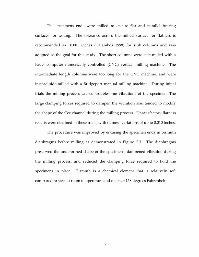
The specimens ends were milled to ensure flat and parallel bearing

surfaces for testing. The tolerance across the milled surface for flatness is

recommended as ±0.001 inches (Galambos 1998) for stub columns and was

adopted as the goal for this study. The short columns were side-milled with a

Fadel computer numerically controlled (CNC) vertical milling machine. The

intermediate length columns were too long for the CNC machine, and were

instead side-milled with a Bridgeport manual milling machine. During initial

trials the milling process caused troublesome vibrations of the specimen. The

large clamping forces required to dampen the vibration also tended to modify

the shape of the Cee channel during the milling process. Unsatisfactory flatness

results were obtained in these trials, with flatness variations of up to 0.010 inches.

The procedure was improved by encasing the specimen ends in bismuth

diaphragms before milling as demonstrated in Figure 2.3. The diaphragms

preserved the undeformed shape of the specimens, dampened vibration during

the milling process, and reduced the clamping force required to hold the

specimens in place. Bismuth is a chemical element that is relatively soft

compared to steel at room temperature and melts at 158 degrees Fahrenheit.

9

Figure 2.3 362S162-33 short column specimen with bismuth end diaphragms

Liquid bismuth was poured into custom wood forms at the specimen

ends. Once the bismuth was set, the specimen (with bismuth end diaphragms)

was positioned in the milling machine (Figure 2.4 through Figure 2.7). Several

passes were made until the steel cross section and bismuth diaphragm were

milled flush. Both column ends were milled without removing the specimen

from the milling table to reduce the chances of unparallel bearing ends. The

bismuth diaphragms were removed from the specimen ends with a few taps of a

wooden mallet and then remelted for the next specimen. The flatness tolerance

of ±0.001 inches was achieved for all but four specimens (see Section 2.3.3.4). A

future improvement to the specimen end preparation could be to use a face mill

instead of an end mill, since the end mill is essentially a cantilever with some

inherent flexibility.

10

Figure 2.4 600S162-33 short column specimen oriented in CNC machine

Figure 2.5 An end mill is used to prepare the column specimens

11

Figure 2.6 The intermediate length specimens were end milled in a manual milling machine

Figure 2.7 The specimens are clamped at the webs only to avoid distortion of the cross section

12

2.3.3 Column Specimen Measurements and Dimensions

2.3.3.1 Dimension Nomenclature

All column dimensions are measured with reference to the orientation of

the specimen in the testing machine. A definition of the assumed reference

system and the specimen dimension nomenclature is provided in Figure 2.8.

RB1

RT1 RT2

RB2

tf1

tw

tf2West East

West East

D1

B1

H

B2

D2

F1 F2

S1 S2

Orientation in testing machine(front view)

EastWest

South

North

L

a a

Section a-a

Figure 2.8 Specimen measurement nomenclature Definitions for the specimen dimension abbreviations are summarized in Table 2.2.

13

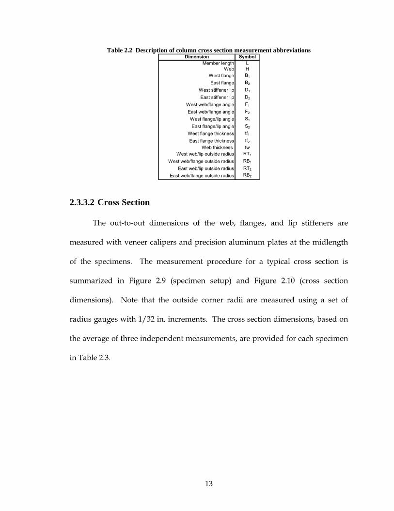
Table 2.2 Description of column cross section measurement abbreviations Dimension Symbol

Member length LWeb H

West flange B1

East flange B2

West stiffener lip D1

East stiffener lip D2

West web/flange angle F1

East web/flange angle F2

West flange/lip angle S1

East flange/lip angle S2

West flange thickness tf1East flange thickness tf2

Web thickness twWest web/lip outside radius RT1

West web/flange outside radius RB1

East web/lip outside radius RT2

East web/flange outside radius RB2

2.3.3.2 Cross Section

The out-to-out dimensions of the web, flanges, and lip stiffeners are

measured with veneer calipers and precision aluminum plates at the midlength

of the specimens. The measurement procedure for a typical cross section is

summarized in Figure 2.9 (specimen setup) and Figure 2.10 (cross section

dimensions). Note that the outside corner radii are measured using a set of

radius gauges with 1/32 in. increments. The cross section dimensions, based on

the average of three independent measurements, are provided for each specimen

in Table 2.3.

14

Check levelness of measuring platform with the angle indicator. The slope perpendicular to the length of the specimen should be as close to zero as possible.

Clamp the specimen to the measuring platform.

Find and mark the longitudinal midline of the specimen.

Figure 2.9 Setup procedure for measuring specimen cross section dimensions

15

Clamp a beveled aluminum plate to the flange. Use the veneer caliper to measure the distance between the edge of the lip and the outside face of the beveled plate. The true dimension (D1 or D2) is then found by subtracting the thickness of the beveled plate from the veneer caliper reading.

Clamp beveled alumninum plates to the lip and web, ofsetting them longituinally by about 1/2 inch. Make sure that the beveled faces are oriented so that they are touching the channel.

Use the extension on the veneer caliper to measure the distance between the outside face of the lip plate and the inside face of the web plate. Make sure that the extension is flush with the flange surface. The true dimension (B1 or B2) is found by subtracting the the thickness of the beveled plate from the veneer caliper reading.

Clamp beveled alumninum plates to each flange, ofsetting them longituinally by about 1/2 inch. Make sure that the beveled faces are oriented so that they are touching the channel.

Use the extension on the veneer caliper to measure the distance between the outside face of one flange plate and the inside face of the other flange plate. Make sure that the extension is flush with the web surface. The true dimension H is found by subtracting the the thickness of the beveled plate from the veneer caliper reading.

Figure 2.10 Procedure for measuring specimen cross section dimensions

16

Clamp beveled aluminum plate to flange.

Measure the flange angle with the angle indicator (F1 and F2).

Clamp the beveled aluminum plate to the stiffener lip. Measure the flange angle using the angle indicator (S1 and S2).

Figure 2.11 Procedure for measuring flange-lip and flange-web angles

The four corner angles of each Cee channel are measured with a digital

angle indicator as demonstrated in Figure 2.11. The angle indicator has a

precision of 0.1 degrees. The flange-lip angles S1 and S2 are measured at the

midlength of the specimens. The web-flange angles F1 and F2 are measured at

several points along the specimen, and will be used in future nonlinear finite

17

element models to simulate initial distortional imperfections. The Cee channel

corner angle magnitudes, based on the average of two independent

measurements, are provided for each specimen in Table 2.4.

Table 2.3 Summary of measured cross section dimensions

H B1 B2 D1 D2 RT1 RT2 RB1 RB2

in. in. in. in. in. in. in. in. in.362-1-24-NH 3.654 1.550 1.621 0.411 0.431 0.188 0.188 0.172 0.188362-2-24-NH 3.712 1.586 1.585 0.416 0.422 0.172 0.203 0.266 0.281362-3-24-NH 3.623 1.677 1.679 0.425 0.399 0.188 0.172 0.281 0.281362-1-24-H 3.583 1.650 1.595 0.430 0.437 0.188 0.203 0.281 0.281362-2-24-H 3.645 1.627 1.593 0.440 0.391 0.188 0.188 0.281 0.281362-3-24-H 3.672 1.674 1.698 0.418 0.426 0.188 0.188 0.266 0.266362-1-48-NH 3.624 1.611 1.605 0.413 0.426 0.172 0.172 0.281 0.281362-2-48-NH 3.624 1.609 1.585 0.407 0.421 0.188 0.172 0.297 0.281362-3-48-NH 3.614 1.604 1.599 0.425 0.401 0.188 0.188 0.266 0.266362-1-48-H 3.622 1.602 1.595 0.420 0.412 0.172 0.172 0.281 0.281362-2-48-H 3.623 1.594 1.610 0.425 0.403 0.172 0.172 0.281 0.281362-3-48-H 3.633 1.604 1.610 0.395 0.432 0.172 0.172 0.281 0.250600-1-24-NH 6.037 1.599 1.631 0.488 0.365 0.172 0.156 0.250 0.203600-2-24-NH 6.070 1.582 1.614 0.472 0.380 0.203 0.203 0.266 0.266600-3-24-NH 6.030 1.601 1.591 0.369 0.483 0.156 0.172 0.266 0.219600-1-24-H 6.040 1.594 1.606 0.484 0.359 0.172 0.172 0.250 0.219600-2-24-H 6.011 1.608 1.602 0.369 0.500 0.172 0.172 0.203 0.234600-3-24-H 6.032 1.606 1.577 0.360 0.478 0.172 0.172 0.250 0.203600-1-48-NH 6.018 1.621 1.609 0.486 0.374 0.172 0.172 0.234 0.219600-2-48-NH 6.017 1.596 1.601 0.482 0.357 0.172 0.172 0.234 0.234600-3-48-NH 6.026 1.585 1.627 0.489 0.338 0.172 0.172 0.266 0.219600-1-48-H 6.010 1.598 1.625 0.480 0.388 0.188 0.156 0.250 0.219600-2-48-H 6.017 1.589 1.607 0.476 0.356 0.172 0.172 0.234 0.234600-3-48-H 6.062 1.632 1.588 0.366 0.480 0.172 0.172 0.219 0.250

Specimen

18

Table 2.4 Summary of measured lip-flange and flange-web cross section angles

X S1 S2 X F1 F2 X F1 F2 X F1 F2 X F1 F2 X F1 F2in. degrees degrees in. degrees degrees in. degrees degrees in. degrees degrees in. degrees degrees in. degrees degrees

362-1-24-NH 12 12.767 8.367 6 82.600 84.500 12 86.033 86.833 18 84.533 87.000362-2-24-NH 12 11.367 11.567 6 86.800 84.800 12 87.600 85.467 18 86.400 83.700362-3-24-NH 12 9.567 9.433 6 85.700 85.000 12 86.300 85.400 18 85.600 83.000362-1-24-H 12 11.130 10.930 6 83.200 83.970 12 87.600 85.600 18 84.330 86.430362-2-24-H 12 4.367 10.267 6 86.000 85.133 12 86.333 85.167 18 84.400 84.500362-3-24-H 12 10.533 10.833 6 85.200 86.333 12 87.700 86.133 18 87.667 89.033362-1-48-NH 12 7.800 10.100 12 85.100 85.600 18 84.300 85.000 24 85.000 85.600 30 84.000 85.200 36 85.300 85.700362-2-48-NH 12 8.000 10.800 12 85.500 84.900 18 84.800 85.100 24 84.200 84.600 30 84.800 85.300 36 85.200 84.900362-3-48-NH 12 9.100 12.200 12 86.900 84.000 18 85.800 83.900 24 85.300 84.100 30 86.400 83.400 36 86.100 83.700362-1-48-H 12 8.500 9.800 12 86.500 84.800 18 86.600 85.000 24 85.600 84.200 30 85.500 85.100 36 86.400 84.400362-2-48-H 12 8.300 11.200 12 86.800 84.800 18 86.500 84.200 24 85.600 83.800 30 85.500 84.100 36 86.700 83.800362-3-48-H 12 9.700 7.300 12 94.700 94.800 18 95.300 93.900 24 95.900 94.700 30 84.400 84.700 36 85.200 85.000600-1-24-NH 24 1.567 2.133 6 90.567 92.033 12 87.533 86.267 18 91.433 93.767600-2-24-NH 24 1.733 2.333 6 91.000 92.033 12 88.833 85.933 18 91.467 93.333600-3-24-NH 24 -2.167 3.500 6 93.700 89.767 12 85.933 88.967 18 92.733 89.667600-1-24-H 24 0.967 2.033 6 89.000 91.000 12 90.400 92.267 18 91.200 92.600600-2-24-H 24 1.800 1.100 6 94.433 90.900 12 93.233 88.733 18 91.967 89.000600-3-24-H 24 0.100 4.100 6 93.500 90.000 12 93.300 89.300 18 90.100 86.300600-1-48-NH 24 0.167 1.400 12 91.033 92.933 18 90.833 92.700 24 90.600 92.800 30 91.333 92.900 36 91.667 93.200600-2-48-NH 24 2.000 2.367 12 90.767 91.900 18 90.233 92.300 24 89.900 91.867 30 90.967 92.000 36 91.467 92.767600-3-48-NH 24 2.600 2.300 12 90.000 92.100 18 89.200 91.900 24 90.000 92.100 30 90.700 92.600 36 90.900 92.500600-1-48-H 24 2.533 2.100 12 90.933 92.167 18 91.000 92.767 24 90.000 92.633 30 91.000 92.000 36 91.100 92.967600-2-48-H 24 2.400 1.000 12 89.000 90.700 18 89.200 91.000 24 88.900 91.200 30 89.600 91.600 36 90.200 92.200600-3-48-H 24 0.667 3.633 12 93.067 89.400 18 93.000 89.500 24 92.300 89.433 30 93.467 89.900 36 93.467 89.600

Specimen

19

2.3.3.3 Specimen Thickness

Sheet metal thickness for each specimen is measured from tensile coupons

cut from the west flange, east flange, and web of an untested section of channel.

All structural studs in this study were delivered by the manufacturer with a zinc

outer coating for galvanic corrosion protection. The sheet metal thickness with

the zinc coating and the bare metal thickness are both useful quantities and are

recorded in this study. The thickness of the zinc coating will be used when

deriving the centerline dimensions of the specimens from the measured out-to-

out dimensions (See Section 2.3.3.2) for use in future finite element models. The

bare metal thickness is used to calculate the steel yield stress in Section 2.3.4.

The sheet steel thickness measurements are made to a precision of 0.0001

inches with a digital micrometer fitted with a thimble friction clutch. The

thickness is determined by averaging five measurements taken within the gauge

length of the tensile coupon (see Figure 2.19 for the definition of gauge length).

The bare sheet metal thicknesses tw, tf1, and tf2 and the zinc coating thickness for

each specimen are summarized in Table 2.5. The average zinc coating thickness

for all specimens is 0.0026 inches.

20

Table 2.5 Specimen bare steel and zinc coating thicknesses

twZinc

thicknesstf1

Zinc thickness

tf2Zinc

thickness

in. in. in. in. in. in.362-1-24-NH362-2-24-NH362-3-24-NH362-1-24-H 0.0390 0.0030 0.0391 0.0034 0.0391 0.0028362-2-24-H 0.0368 0.0057 0.0390 0.0023 0.0391 0.0034362-3-24-H 0.0394 0.0027 0.0394 0.0018 0.0394 0.0026362-1-48-NH 0.0392 0.0025 0.0393 0.0020 0.0392 0.0020362-2-48-NH 0.0393 0.0025 0.0394 0.0022 0.0393 0.0026362-3-48-NH 0.0389 0.0013 0.0391 0.0009 0.0390 0.0017362-1-48-H 0.0391 0.0019 0.0393 0.0017 0.0394 0.0017362-2-48-H 0.0390 N/M 0.0391 N/M 0.0391 N/M362-3-48-H 0.0401 0.0000 0.0400 0.0000 0.0397 0.0010600-1-24-NH600-2-24-NH600-3-24-NH600-1-24-H 0.0414 0.0042 0.0422 0.0044 0.0428 0.0030600-2-24-H 0.0427 0.0039 0.0384 0.0084 0.0424 0.0042600-3-24-H 0.0429 0.0031 0.0431 0.0026 0.0430 0.0036600-1-48-NH 0.0434 0.0026 0.0436 0.0024 0.0434 0.0028600-2-48-NH 0.0435 0.0017 0.0430 0.0024 0.0430 0.0023600-3-48-NH 0.0436 0.0015 0.0432 0.0021 0.0433 0.0020600-1-48-H 0.0429 0.0022 0.0426 0.0023 0.0429 0.0021600-2-48-H 0.0429 N/M 0.0428 N/M 0.0431 N/M600-3-48-H 0.0430 N/M 0.0434 N/M 0.0430 N/M

NOTE: N/M Not measured

Web West Flange East Flange

Specimen

0.0302 N/M

0.0438 N/M 0.0432 N/M 0.0438 N/M

0.0368 0.0372N/M N/M

The zinc coating is removed by immersing the tensile coupons in a ferric

chloride bath for 100 minutes. The immersion time was determined with a study

of coupon thickness variation over time for the 362-2-24-H Web and the 600-2-24-

H West Flange tensile coupons. The coupons were removed from the ferric

chloride bath every 10 minutes, cleaned, and then measured. Figure 2.12

demonstrates that the coupon thickness converges to a constant value, the base

metal thickness, at approximately 100 minutes.

21

0 0.2 0.4 0.6 0.8 10

0.2

0.4

0.6

0.8

1

0 20 40 60 80 100 1200

0.2

0.4

0.6

0.8

1

1.2

1.4

time (minutes)

coup

on th

ickn

ess/

initi

al th

ickn

ess

362-2-24-H Web Coupon600-2-24-H West Flange Coupon

Figure 2.12 Removal of tensile coupon zinc coating as a function of time

2.3.3.4 Specimen Flatness and Length

After each specimen is saw cut and milled flat, a vertical height gauge

with a precision of 0.001 inches is used to measure the specimen length and

flatness (Figure 2.13). For each specimen, two independent length measurements

are taken at each rounded corner location described in Figure 2.14. The four

length measurements provide information on the flatness of the specimen ends.

The height gauge and specimen are placed on the same steel table to ensure that

all measurements are made in the same reference plane. The steel table was

checked for flatness with a dial gauge and precision stand before measurements

proceeded. It was determined that the table is flatter than the precision of the

height gauge and was therefore an acceptable surface for obtaining length

22

measurements. Lengths LRT1, LRT2, LRB1, and LRB2 as well as the average

length L are provided for each specimen in Table 2.6. The specimen flatness,

defined as the difference between LRT1, LRT2, LRB1, and LRB2 and the average

length L, is reported in Table 2.7. All but four specimens meet the flatness

tolerance of ±0.001 inches, with short column 362-2-48-H having the maximum

deviation of +0.003 inches at LRT2.

North

Figure 2.13 A height gauge is used to measure specimen length

23

LRB1

LRT1 LRT2

LRB2

West East

Figure 2.14 Length is measured at the four corners of the Cee channel

Table 2.6 Measured column specimen length

Specimen LRT1 LRT2 LRB1 LRB2 L (avg.)in. in. in. in. in.

362-1-24-NH 24.100 24.100 24.098 24.099 24.099362-2-24-NH 24.097 24.098 24.099 24.099 24.098362-3-24-NH 24.097 24.098 24.098 24.099 24.098362-1-24-H 24.100 24.099 24.098 24.100 24.099362-2-24-H 24.097 24.099 24.099 24.100 24.099362-3-24-H 24.099 24.099 24.099 24.100 24.099362-1-48-NH 48.214 48.214 48.214 48.214 48.214362-2-48-NH 48.303 48.300 48.301 48.298 48.301362-3-48-NH 48.192 48.19 48.191 48.189 48.191362-1-48-H 48.217 48.216 48.216 48.216 48.216362-2-48-H 48.232 48.232 48.231 48.231 48.232362-3-48-H 48.196 48.200 48.195 48.198 48.197600-1-24-NH 24.100 24.101 24.099 24.099 24.100600-2-24-NH 24.102 24.104 24.102 24.103 24.103600-3-24-NH 24.100 24.098 24.099 24.099 24.099600-1-24-H 24.102 24.100 24.100 24.101 24.101600-2-24-H 24.098 24.099 24.100 24.100 24.099600-3-24-H 24.101 24.101 24.101 24.100 24.101600-1-48-NH 48.255 48.255 48.255 48.255 48.255600-2-48-NH 48.250 48.250 48.250 48.251 48.250600-3-48-NH 48.295 48.294 48.295 48.294 48.295600-1-48-H 48.089 48.088 48.089 48.088 48.089600-2-48-H 48.253 48.251 48.253 48.253 48.253600-3-48-H 48.061 48.061 48.059 48.059 48.060

Specimen Length

24

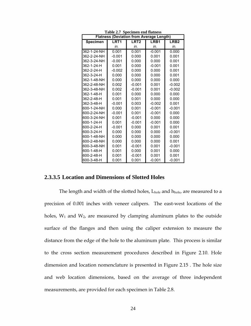
Table 2.7 Specimen end flatness

Specimen LRT1 LRT2 LRB1 LRB2in. in. in. in.

362-1-24-NH 0.001 0.001 -0.001 0.000362-2-24-NH -0.001 0.000 0.001 0.001362-3-24-NH -0.001 0.000 0.000 0.001362-1-24-H 0.001 0.000 -0.001 0.001362-2-24-H -0.002 0.000 0.000 0.001362-3-24-H 0.000 0.000 0.000 0.001362-1-48-NH 0.000 0.000 0.000 0.000362-2-48-NH 0.002 -0.001 0.001 -0.002362-3-48-NH 0.002 -0.001 0.001 -0.002362-1-48-H 0.001 0.000 0.000 0.000362-2-48-H 0.001 0.001 0.000 0.000362-3-48-H -0.001 0.003 -0.002 0.001600-1-24-NH 0.000 0.001 -0.001 -0.001600-2-24-NH -0.001 0.001 -0.001 0.000600-3-24-NH 0.001 -0.001 0.000 0.000600-1-24-H 0.001 -0.001 -0.001 0.000600-2-24-H -0.001 0.000 0.001 0.001600-3-24-H 0.000 0.000 0.000 -0.001600-1-48-NH 0.000 0.000 0.000 0.000600-2-48-NH 0.000 0.000 0.000 0.001600-3-48-NH 0.001 -0.001 0.001 -0.001600-1-48-H 0.001 0.000 0.001 0.000600-2-48-H 0.001 -0.001 0.001 0.001600-3-48-H 0.001 0.001 -0.001 -0.001

Flatness (Deviation from Average Length)

2.3.3.5 Location and Dimensions of Slotted Holes

The length and width of the slotted holes, Lhole and hhole, are measured to a

precision of 0.001 inches with veneer calipers. The east-west locations of the

holes, W1 and W2, are measured by clamping aluminum plates to the outside

surface of the flanges and then using the caliper extension to measure the

distance from the edge of the hole to the aluminum plate. This process is similar

to the cross section measurement procedures described in Figure 2.10. Hole

dimension and location nomenclature is presented in Figure 2.15 . The hole size

and web location dimensions, based on the average of three independent

measurements, are provided for each specimen in Table 2.8.

25

North

aa

W1 W2

X

Section a-a

Lhole

hhole

Front view Figure 2.15 Hole dimension location and size nomenclature

Table 2.8 Measured slotted hole dimensions and locations X W1 W2 L hole d hole X W1 W2 L hole d holein. in. in. in. in. in. in. in. in. in.

362-1-24-H L/2 0.946 1.141 4.003 1.492362-2-24-H L/2 1.146 0.967 4.000 1.502362-3-24-H L/2 0.935 1.114 4.005 1.493362-1-48-H (L-24)/2 1.252 0.974 3.999 1.500 (L+24)/2 1.198 0.952 4.001 1.494362-2-48-H (L-24)/2 1.126 1.016 4.001 1.496 (L+24)/2 1.171 0.973 4.003 1.494362-3-48-H (L-24)/2 0.982 1.112 4.000 1.493 (L+24)/2 0.967 1.133 4.003 1.491600-1-24-H L/2 2.147 2.361 4.002 1.498600-2-24-H L/2 2.365 2.155 4.001 1.491600-3-24-H L/2 2.347 2.166 4.001 1.493600-1-48-H (L-24)/2 2.161 2.375 4.002 1.494 (L+24)/2 2.162 2.383 3.998 1.497600-2-48-H (L-24)/2 2.166 2.351 4.001 1.499 (L+24)/2 2.176 2.360 4.002 1.498600-3-48-H (L-24)/2 2.371 2.162 3.999 1.497 (L+24)/2 2.365 2.156 4.003 1.494

Specimen

26

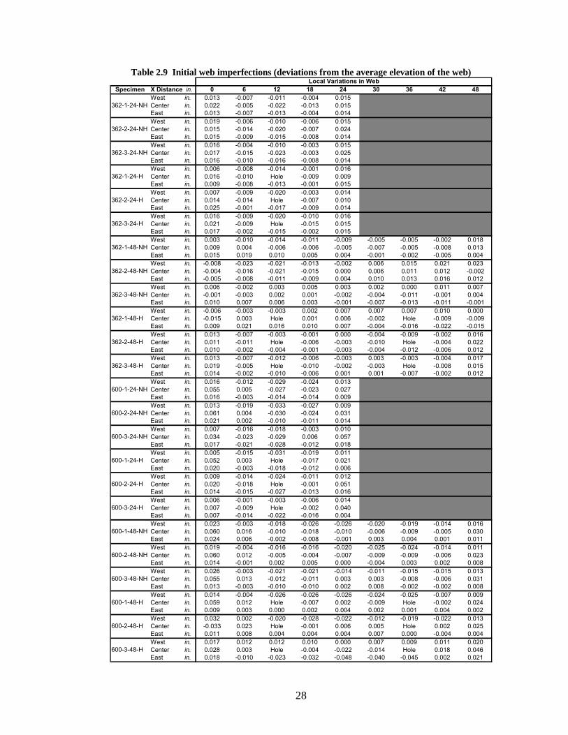
2.3.3.6 Initial Web Imperfections

Variations in the specimen webs are measured to estimate the local

buckling initial imperfection magnitudes to be used in future nonlinear finite

element models of the specimens. The measurements will also identify the

global weak axis sweep of a specimen. The test setup in Figure 2.16 employs a

dial gauge with a precision of 0.001 inches mounted to a laboratory stand in

contact with a flat steel table. The specimen is supported horizontally at both

ends by a matching pair of steel bars that have been ground flat and parallel.

The bars are also in contact with the steel table, ensuring that the specimen and

the dial gauge are in the same horizontal reference plane. Each specimen web is

marked with a grid of measurement points in Figure 2.17. The stand and dial

gauge are shifted from grid point to grid point and elevation measurements are

recorded. The variations in web elevations, based on an average of two

measurements per grid point, are provided for each specimen in Table 2.9. The

variations are calculated using the average elevation of the specimen web as a

baseline.

27

Figure 2.16 A dial gauge and precision stand are used to measure initial web imperfections

North

X

1.2 inches (362 specimens)2.3 inches (600 specimens)

CL Web (typ.)

West Center East

a

a

Section a-a

+ variation

Plan view(short and intermediate length web grid layouts)

6 in. (typ.)

Figure 2.17 Web imperfection measurement grid and coordinate system

28

Table 2.9 Initial web imperfections (deviations from the average elevation of the web)

Specimen X Distance in. 0 6 12 18 24 30 36 42 48West in. 0.013 -0.007 -0.011 -0.004 0.015Center in. 0.022 -0.005 -0.022 -0.013 0.015East in. 0.013 -0.007 -0.013 -0.004 0.014West in. 0.019 -0.006 -0.010 -0.006 0.015Center in. 0.015 -0.014 -0.020 -0.007 0.024East in. 0.015 -0.009 -0.015 -0.008 0.014West in. 0.016 -0.004 -0.010 -0.003 0.015Center in. 0.017 -0.015 -0.023 -0.003 0.025East in. 0.016 -0.010 -0.016 -0.008 0.014West in. 0.006 -0.008 -0.014 -0.001 0.016Center in. 0.016 -0.010 Hole -0.009 0.009East in. 0.009 -0.008 -0.013 -0.001 0.015West in. 0.007 -0.009 -0.020 -0.003 0.014Center in. 0.014 -0.014 Hole -0.007 0.010East in. 0.025 -0.001 -0.017 -0.009 0.014West in. 0.016 -0.009 -0.020 -0.010 0.016Center in. 0.021 -0.009 Hole -0.015 0.015East in. 0.017 -0.002 -0.015 -0.002 0.015West in. 0.003 -0.010 -0.014 -0.011 -0.009 -0.005 -0.005 -0.002 0.018Center in. 0.009 0.004 -0.006 -0.006 -0.005 -0.007 -0.005 -0.008 0.013East in. 0.015 0.019 0.010 0.005 0.004 -0.001 -0.002 -0.005 0.004West in. -0.008 -0.023 -0.021 -0.013 -0.002 0.006 0.015 0.021 0.023Center in. -0.004 -0.016 -0.021 -0.015 0.000 0.006 0.011 0.012 -0.002East in. -0.005 -0.008 -0.011 -0.009 0.004 0.010 0.013 0.016 0.012West in. 0.006 -0.002 0.003 0.005 0.003 0.002 0.000 0.011 0.007Center in. -0.001 -0.003 0.002 0.001 -0.002 -0.004 -0.011 -0.001 0.004East in. 0.010 0.007 0.006 0.003 -0.001 -0.007 -0.013 -0.011 -0.001West in. -0.006 -0.003 -0.003 0.002 0.007 0.007 0.007 0.010 0.000Center in. -0.015 0.003 Hole 0.001 0.006 -0.002 Hole -0.009 -0.009East in. 0.009 0.021 0.016 0.010 0.007 -0.004 -0.016 -0.022 -0.015West in. 0.013 -0.007 -0.003 -0.001 0.000 -0.004 -0.009 -0.002 0.016Center in. 0.011 -0.011 Hole -0.006 -0.003 -0.010 Hole -0.004 0.022East in. 0.010 -0.002 -0.004 -0.001 -0.003 -0.004 -0.012 -0.006 0.012West in. 0.013 -0.007 -0.012 -0.006 -0.003 0.003 -0.003 -0.004 0.017Center in. 0.019 -0.005 Hole -0.010 -0.002 -0.003 Hole -0.008 0.015East in. 0.014 -0.002 -0.010 -0.006 0.001 0.001 -0.007 -0.002 0.012West in. 0.016 -0.012 -0.029 -0.024 0.013Center in. 0.055 0.005 -0.027 -0.023 0.027East in. 0.016 -0.003 -0.014 -0.014 0.009West in. 0.013 -0.019 -0.033 -0.027 0.009Center in. 0.061 0.004 -0.030 -0.024 0.031East in. 0.021 0.002 -0.010 -0.011 0.014West in. 0.007 -0.016 -0.018 -0.003 0.010Center in. 0.034 -0.023 -0.029 0.006 0.057East in. 0.017 -0.021 -0.028 -0.012 0.018West in. 0.005 -0.015 -0.031 -0.019 0.011Center in. 0.052 0.003 Hole -0.017 0.021East in. 0.020 -0.003 -0.018 -0.012 0.006West in. 0.009 -0.014 -0.024 -0.011 0.012Center in. 0.020 -0.018 Hole -0.001 0.051East in. 0.014 -0.015 -0.027 -0.013 0.016West in. 0.006 -0.001 -0.003 -0.006 0.014Center in. 0.007 -0.009 Hole -0.002 0.040East in. 0.007 -0.014 -0.022 -0.016 0.004West in. 0.023 -0.003 -0.018 -0.026 -0.026 -0.020 -0.019 -0.014 0.016Center in. 0.060 0.016 -0.010 -0.018 -0.010 -0.006 -0.009 -0.005 0.030East in. 0.024 0.006 -0.002 -0.008 -0.001 0.003 0.004 0.001 0.011West in. 0.019 -0.004 -0.016 -0.016 -0.020 -0.025 -0.024 -0.014 0.011Center in. 0.060 0.012 -0.005 -0.004 -0.007 -0.009 -0.009 -0.006 0.023East in. 0.014 -0.001 0.002 0.005 0.000 -0.004 0.003 0.002 0.008West in. 0.026 -0.003 -0.021 -0.021 -0.014 -0.011 -0.015 -0.015 0.013Center in. 0.055 0.013 -0.012 -0.011 0.003 0.003 -0.008 -0.006 0.031East in. 0.013 -0.003 -0.010 -0.010 0.002 0.008 -0.002 -0.002 0.008West in. 0.014 -0.004 -0.026 -0.026 -0.026 -0.024 -0.025 -0.007 0.009Center in. 0.059 0.012 Hole -0.007 0.002 -0.009 Hole -0.002 0.024East in. 0.009 0.003 0.000 0.002 0.004 0.002 0.001 0.004 0.002West in. 0.032 0.002 -0.020 -0.028 -0.022 -0.012 -0.019 -0.022 0.013Center in. -0.033 0.023 Hole -0.001 0.006 0.005 Hole 0.002 0.025East in. 0.011 0.008 0.004 0.004 0.004 0.007 0.000 -0.004 0.004West in. 0.017 0.012 0.012 0.010 0.000 0.007 0.009 0.011 0.020Center in. 0.028 0.003 Hole -0.004 -0.022 -0.014 Hole 0.018 0.046East in. 0.018 -0.010 -0.023 -0.032 -0.048 -0.040 -0.045 0.002 0.021

362-1-24-NH

362-2-24-NH

362-3-24-NH

362-1-24-H

362-2-48-H

362-3-48-H

362-2-24-H

362-3-24-H

362-1-48-NH

362-2-48-NH

600-3-48-H

600-2-24-H

600-3-24-H

600-1-48-NH

600-2-48-NH

Local Variations in Web

600-3-48-NH

600-1-48-H

600-2-48-H

600-1-24-NH

600-2-24-NH

600-3-24-NH

600-1-24-H

362-3-48-NH

362-1-48-H

29

2.3.4 Materials Testing

The steel stress-strain curve and yield stress are determined for the web,

west flange, and east flange of each specimen in this study. The material

properties are determined with tensile coupon tests in accordance with the

ASTM specification E 8M-04, “Standard Test Methods for Tension Testing of

Metallic Materials (Metric)” (ASTM 2004).

2.3.4.1 Coupon Preparation

The tensile coupons are always obtained from the same 8 ft. structural

stud that produced the column specimen. Flat portions of the web and flanges

are first rough cut with a metal ban saw (Figure 2.18), and then finished to the

dimensions in Figure 2.19 with a CNC milling machine. The special jig in Figure

2.19 allowed for three tensile coupons to be milled at once. The tensile coupons

were stripped of their zinc coating (see Section 2.3.3.3 for procedure) and then

measured within the gauge length for bare metal thickness, t, and minimum

width, wmin. The metal thickness measurement procedures are described in

Section 2.3.3.3 of this report. The minimum width is determined by taking the

minimum of five independent measurements within the gauge length of the

specimen with a micrometer.

30

Figure 2.18 Tensile coupons are first rough cut with a metal ban saw

0.79 in.

1.97 in.

1.97 in.

3.18 in. 1.97 in.

0.38 in.0.38 in.

R=0.55 in.

0.492 in. *

gauge length

*nominal, actual dimension will vary slightly

Figure 2.19 Tensile coupon dimensions as entered in the CNC milling machine computer

31

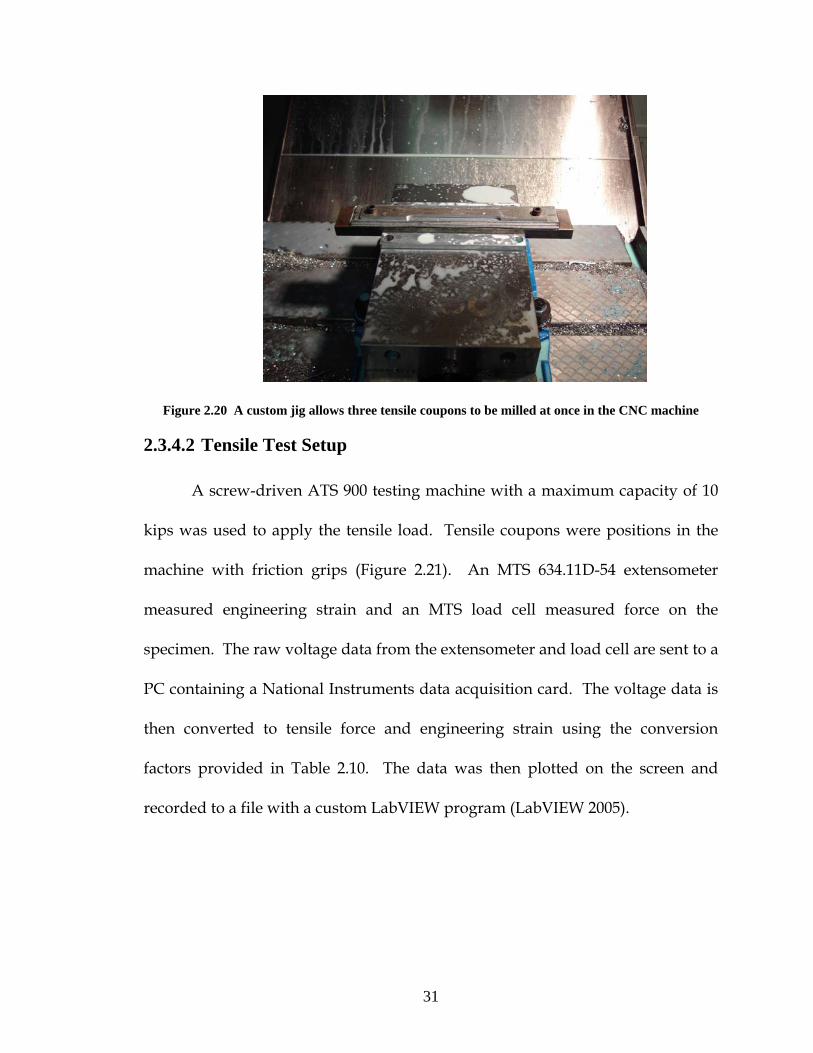
Figure 2.20 A custom jig allows three tensile coupons to be milled at once in the CNC machine

2.3.4.2 Tensile Test Setup

A screw-driven ATS 900 testing machine with a maximum capacity of 10

kips was used to apply the tensile load. Tensile coupons were positions in the

machine with friction grips (Figure 2.21). An MTS 634.11D-54 extensometer

measured engineering strain and an MTS load cell measured force on the

specimen. The raw voltage data from the extensometer and load cell are sent to a

PC containing a National Instruments data acquisition card. The voltage data is

then converted to tensile force and engineering strain using the conversion

factors provided in Table 2.10. The data was then plotted on the screen and

recorded to a file with a custom LabVIEW program (LabVIEW 2005).

32

Figure 2.21 ATS machine used to test tensile coupons

Table 2.10 Voltage conversion factors for tensile coupon testing

Measurement Source Conversion

Tensile Force MTS Load Cell 1 Volt = 3.96x10-5 strain (in./in.)

Engineering Strain MTS Extensometer 1 Volt = 1000 lbf

Tensile Coupon Testing

2.3.4.3 Tensile Test Results

Two distinct types of steel stress-strain curves are observed for the tensile

coupons in this study. Tensile coupons from the 362S162-33 structural studs

demonstrate gradual yielding behavior, while the tensile coupons from the

33

600S162-33 studs demonstrate a sharp yielding plateau. The yield stress, fy ,for

the gradually yielding specimens is determined with the 0.2% strain offset

method. The stress-strain curve for specimen 362-3-48-NH (East Flange)

demonstrates the offset method in Figure 2.22. The yield stress for the sharply

yielding specimens is determined by averaging the stresses in the yield plateau.

The averaging range is determined by using two strain offset lines, one at 0.4%

strain offset and the other at 0.8% offset. The stress-strain curve for specimen

600-24-NH (West Flange) in Figure 2.23 demonstrates this autographic method.

The steel modulus of elasticity, E, is assumed as 29500 ksi for all specimens when

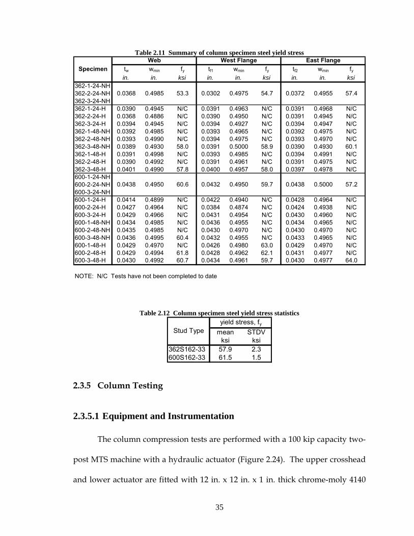
determining the yield stress. The tensile coupon yield stresses and cross section

dimensions are summarized in Table 2.11. The mean and standard deviation for

all 362S162-33 and 600S162-33 tensile coupons tested to date are provided in

Table 2.12.

34

0 0.2 0.4 0.6 0.8 10

0.2

0.4

0.6

0.8

1

0 0.05 0.1 0.15 0.2 0.250

10

20

30

40

50

60

70

80

90

100

Engineering Strain,(in./in.)

Axi

al T

ensi

le S

tress

(ksi

)

YIELD STRESS (0.2% offset)=60.1 ksi

0.2% strain offset line (slope=29500 ksi)

Figure 2.22 Gradually yielding stress-strain curve with 0.2% strain offset method for determining fy

0 0.2 0.4 0.6 0.8 10

0.2

0.4

0.6

0.8

1

0 0.05 0.1 0.15 0.2 0.250

10

20

30

40

50

60

70

80

90

100

Engineering Strain (in./in.)

Axi

al T

ensi

le S

tress

(ksi

)

YIELD STRESS (Autographic Method)=59.7 ksi

0.4% strain offset line (slope=29500 ksi)

0.8% strain offset line (slope=29500 ksi)

Figure 2.23 Sharp-yielding stress strain curve using an autographic method for determining fy

35

Table 2.11 Summary of column specimen steel yield stress

tw wmin fy tf1 wmin fy tf2 wmin fyin. in. ksi in. in. ksi in. in. ksi

362-1-24-NH362-2-24-NH362-3-24-NH362-1-24-H 0.0390 0.4945 N/C 0.0391 0.4963 N/C 0.0391 0.4968 N/C362-2-24-H 0.0368 0.4886 N/C 0.0390 0.4950 N/C 0.0391 0.4945 N/C362-3-24-H 0.0394 0.4945 N/C 0.0394 0.4927 N/C 0.0394 0.4947 N/C362-1-48-NH 0.0392 0.4985 N/C 0.0393 0.4965 N/C 0.0392 0.4975 N/C362-2-48-NH 0.0393 0.4990 N/C 0.0394 0.4975 N/C 0.0393 0.4970 N/C362-3-48-NH 0.0389 0.4930 58.0 0.0391 0.5000 58.9 0.0390 0.4930 60.1362-1-48-H 0.0391 0.4998 N/C 0.0393 0.4985 N/C 0.0394 0.4991 N/C362-2-48-H 0.0390 0.4992 N/C 0.0391 0.4961 N/C 0.0391 0.4975 N/C362-3-48-H 0.0401 0.4990 57.8 0.0400 0.4957 58.0 0.0397 0.4978 N/C600-1-24-NH600-2-24-NH600-3-24-NH600-1-24-H 0.0414 0.4899 N/C 0.0422 0.4940 N/C 0.0428 0.4964 N/C600-2-24-H 0.0427 0.4964 N/C 0.0384 0.4874 N/C 0.0424 0.4938 N/C600-3-24-H 0.0429 0.4966 N/C 0.0431 0.4954 N/C 0.0430 0.4960 N/C600-1-48-NH 0.0434 0.4985 N/C 0.0436 0.4955 N/C 0.0434 0.4965 N/C600-2-48-NH 0.0435 0.4985 N/C 0.0430 0.4970 N/C 0.0430 0.4970 N/C600-3-48-NH 0.0436 0.4995 60.4 0.0432 0.4955 N/C 0.0433 0.4965 N/C600-1-48-H 0.0429 0.4970 N/C 0.0426 0.4980 63.0 0.0429 0.4970 N/C600-2-48-H 0.0429 0.4994 61.8 0.0428 0.4962 62.1 0.0431 0.4977 N/C600-3-48-H 0.0430 0.4992 60.7 0.0434 0.4961 59.7 0.0430 0.4977 64.0

NOTE: N/C Tests have not been completed to date

0.4955

0.0438 0.04380.0432

0.4985 53.3 57.40.4975 54.7

SpecimenWeb East FlangeWest Flange

0.0368 0.03720.0302

0.4950 60.6 0.5000 57.20.4950 59.7

Table 2.12 Column specimen steel yield stress statistics

mean STDVksi ksi

362S162-33 57.9 2.3600S162-33 61.5 1.5

yield stress, fyStud Type

2.3.5 Column Testing

2.3.5.1 Equipment and Instrumentation

The column compression tests are performed with a 100 kip capacity two-

post MTS machine with a hydraulic actuator (Figure 2.24). The upper crosshead

and lower actuator are fitted with 12 in. x 12 in. x 1 in. thick chrome-moly 4140

36

steel platens that have been ground flat and parallel. An MTS load cell (model

number 661-23A-02) measures the applied compressive force on the specimen,

and the internal MTS length-voltage displacement transducer (LVDT) reports

actuator displacement. An MTS 407 controller is used to operate the hydraulic

actuator while orienting the specimen and during the compression tests.

MTS Load CellFixed Crosshead

Steel Platen

Novotechnikposition transducers (with magnet tips)

Hydraulic actuator

Figure 2.24 Column test setup and instrumentation

Magnetic tip

Figure 2.25 Novotechnik position transducer with ball-jointed magnetic tip

37

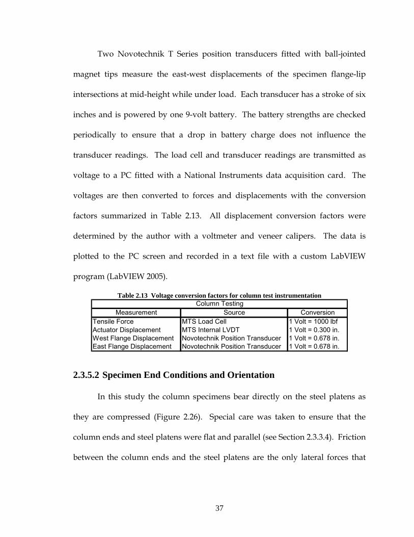
Two Novotechnik T Series position transducers fitted with ball-jointed

magnet tips measure the east-west displacements of the specimen flange-lip

intersections at mid-height while under load. Each transducer has a stroke of six

inches and is powered by one 9-volt battery. The battery strengths are checked

periodically to ensure that a drop in battery charge does not influence the

transducer readings. The load cell and transducer readings are transmitted as

voltage to a PC fitted with a National Instruments data acquisition card. The

voltages are then converted to forces and displacements with the conversion

factors summarized in Table 2.13. All displacement conversion factors were

determined by the author with a voltmeter and veneer calipers. The data is

plotted to the PC screen and recorded in a text file with a custom LabVIEW

program (LabVIEW 2005).

Table 2.13 Voltage conversion factors for column test instrumentation

Measurement Source ConversionTensile Force MTS Load Cell 1 Volt = 1000 lbfActuator Displacement MTS Internal LVDT 1 Volt = 0.300 in.West Flange Displacement Novotechnik Position Transducer 1 Volt = 0.678 in.East Flange Displacement Novotechnik Position Transducer 1 Volt = 0.678 in.

Column Testing

2.3.5.2 Specimen End Conditions and Orientation

In this study the column specimens bear directly on the steel platens as

they are compressed (Figure 2.26). Special care was taken to ensure that the

column ends and steel platens were flat and parallel (see Section 2.3.3.4). Friction

between the column ends and the steel platens are the only lateral forces that

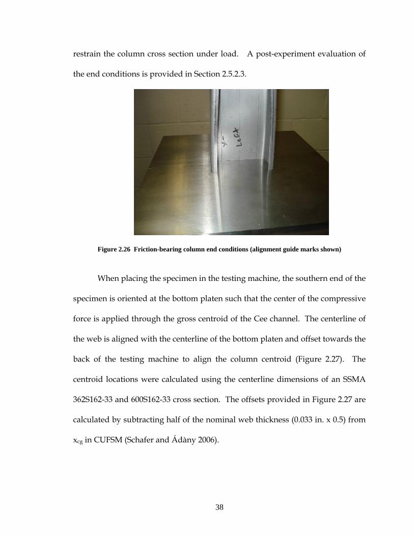
38

restrain the column cross section under load. A post-experiment evaluation of

the end conditions is provided in Section 2.5.2.3.

Figure 2.26 Friction-bearing column end conditions (alignment guide marks shown)

When placing the specimen in the testing machine, the southern end of the

specimen is oriented at the bottom platen such that the center of the compressive

force is applied through the gross centroid of the Cee channel. The centerline of

the web is aligned with the centerline of the bottom platen and offset towards the

back of the testing machine to align the column centroid (Figure 2.27). The

centroid locations were calculated using the centerline dimensions of an SSMA

362S162-33 and 600S162-33 cross section. The offsets provided in Figure 2.27 are

calculated by subtracting half of the nominal web thickness (0.033 in. x 0.5) from

xcg in CUFSM (Schafer and Ádàny 2006).

39

Plan View(Bottom Platen)

CL Platen and Column Web

0.380 in. (600S162-33)0.502 in. (362S162-33)

CL Platen

Location of interior web edge

Center of platen, center of load, centroid of Ceechannel

FRONT OF MTS MACHINE

Column specimen

Figure 2.27 Column specimen alignment schematic

The actual cross section and thickness measurements produce centroid

offsets slightly different from the nominal offsets considered in the column tests.

The difference between the nominal and measured offsets, defined here as ΔCG,

are provided in Table 2.14. ΔCG produces end moments in the specimens that

are several orders of magnitude smaller than the applied loads in this study. For

example, the end moments created by a ΔCG of 0.059 inches for specimen 600-3-

24-NH are calculated as 2.0 x 10-6 kip*inches at peak load (Ptest=12.24 kips) using

the structural analysis program MASTAN (Ziemian and McGuire 2005). The

assumed MASTAN structural system in Figure 2.28 shows that relatively stiff

40

compression platens and fixed-fixed end conditions effectively eliminate end

moments from small load eccentricities.

Table 2.14 Specimen gross centroids and offset from applied load during tests

ΔCSxcg tz xcg - tz used in testsin. in. in. in. in.

362-1-24-NH 0.482 0.038 0.463 0.502 0.039362-2-24-NH 0.471 0.038 0.452 0.502 0.050362-3-24-NH 0.504 0.038 0.485 0.502 0.017362-1-24-H 0.511 0.042 0.489 0.502 0.013362-2-24-H 0.490 0.042 0.469 0.502 0.033362-3-24-H 0.524 0.042 0.503 0.502 -0.001362-1-48-NH 0.475 0.041 0.454 0.502 0.048362-2-48-NH 0.468 0.042 0.447 0.502 0.055362-3-48-NH 0.475 0.040 0.455 0.502 0.047362-1-48-H 0.470 0.041 0.449 0.502 0.053362-2-48-H 0.470 0.042 0.449 0.502 0.053362-3-48-H 0.486 0.040 0.466 0.502 0.036600-1-24-NH 0.354 0.047 0.330 0.380 0.050600-2-24-NH 0.347 0.047 0.323 0.380 0.057600-3-24-NH 0.344 0.047 0.321 0.380 0.059600-1-24-H 0.363 0.046 0.340 0.380 0.040600-2-24-H 0.368 0.047 0.344 0.380 0.036600-3-24-H 0.361 0.046 0.338 0.380 0.042600-1-48-NH 0.362 0.046 0.339 0.380 0.041600-2-48-NH 0.355 0.045 0.333 0.380 0.047600-3-48-NH 0.353 0.045 0.330 0.380 0.050600-1-48-H 0.362 0.045 0.340 0.380 0.040600-2-48-H 0.352 0.046 0.329 0.380 0.051600-3-48-H 0.356 0.046 0.333 0.380 0.047

tz sheet thickness with zinc coatingΔCS difference measured and as tested centroid offsets

Specimen Measurements Centroid Shift

Centroid Shift

Specimen

41

Actuator load

Column specimen

(Centroid shown)

ΔCG

Platen (typ.)

Horizontal translation and rotational DOF restrained

CL Applied Load

Stiff platen Flexible platen

Structural System Moment Diagrams

No moment in column for stiff platen even with load offset

All translation and rotational DOF restrained

Figure 2.28 Influence of platen bending stiffness on end moments for a fixed-fixed eccentric column

Once the specimen is aligned on the bottom platen, 500 lbs of compressive

force was applied to the column and weak-axis out of straightness measurements

were taken. The distance from the front of the top and bottom platens to the

interior web edge is denoted as Stop and Sbottom in Figure 2.30. These values are

initially taken as the average of three independent measurements with a veneer

caliper (Figure 2.29) and then corrected for the platen offset (Figure 2.30) and the

initial web imperfections in Table 2.9. The revised Stop and Sbottom with respect to

42

the average plane of the web is then used to calculate the initial out-of-

straightness measurement ΔS provided in Table 2.15. This information will be

incorporated into future nonlinear finite element models of the specimens as an

initial out-of-straightness column imperfection.

Figure 2.29 Veneer calipers are used to measure the distance from the column web to the platen edge

43

a a

Sbottom

Stop

Stop

Section a-a

Column Specimen(orientation exaggerated)

Front of MTS Machine

Side View(Looking west)

CL Platen

CL Platen

CL Load

ΔS (negative magnitude shown)

Platen Offset=0.084 in.

Figure 2.30 Column specimen weak axis out-of-straightness schematic

Table 2.15 Summary of out-of-straightness calculations Specimen Sbottom Stop Platen Offset Sbottom Correction Sbottom Correction Stop ΔS

As measured

As measured

Top platen edge is offset from bottom

platen edge

Corrected for top platen

offset

Web Imperfection @

X=0

Corrected for Web

Imperfection @ X=0

Web Imperfection @

X=L

Corrected for Web

Imperfection @ X=L

Initial out of straightness

in. in. in. in. in. in. in. in. in.362-1-24-NH 6.507 6.622 0.084 6.591 0.015 6.577 0.022 6.600 -0.024362-2-24-NH 6.523 6.612 0.084 6.607 0.015 6.593 0.024 6.588 0.004362-3-24-NH 6.531 6.585 0.084 6.615 0.017 6.598 0.025 6.560 0.038362-1-24-H 6.524 6.613 0.084 6.608 0.016 6.592 0.009 6.604 -0.012362-2-24-H 6.532 6.578 0.084 6.616 0.014 6.602 0.010 6.568 0.034362-3-24-H 6.529 6.629 0.084 6.613 0.021 6.592 0.015 6.615 -0.023362-1-48-NH 6.352 6.393 0.084 6.436 0.009 6.427 0.013 6.380 0.047362-2-48-NH 6.535 6.649 0.084 6.619 -0.004 6.623 -0.002 6.651 -0.028362-3-48-NH 6.537 6.614 0.084 6.621 -0.001 6.622 0.004 6.610 0.012362-1-48-H 6.530 6.554 0.084 6.614 -0.015 6.629 -0.009 6.563 0.066362-2-48-H 6.534 6.617 0.084 6.618 0.011 6.607 0.022 6.594 0.013362-3-48-H 6.532 6.616 0.084 6.616 0.019 6.598 0.015 6.601 -0.003600-1-24-NH 6.352 6.472 0.084 6.436 0.055 6.381 0.027 6.444 -0.063600-2-24-NH 6.365 6.560 0.084 6.449 0.061 6.388 0.031 6.529 -0.141600-3-24-NH 6.451 6.494 0.084 6.535 0.034 6.501 0.057 6.437 0.063600-1-24-H 6.356 6.486 0.084 6.440 0.052 6.388 0.021 6.466 -0.078600-2-24-H 6.360 6.399 0.084 6.444 0.020 6.424 0.051 6.348 0.076600-3-24-H 6.355 6.403 0.084 6.439 0.007 6.432 0.040 6.363 0.069600-1-48-NH 6.346 6.436 0.084 6.430 0.060 6.370 0.030 6.406 -0.036600-2-48-NH 6.354 6.488 0.084 6.438 0.060 6.377 0.023 6.465 -0.087600-3-48-NH 6.354 6.463 0.084 6.438 0.055 6.383 0.031 6.432 -0.049600-1-48-H 6.311 6.458 0.084 6.395 0.059 6.336 0.024 6.433 -0.098600-2-48-H 6.352 6.422 0.084 6.436 -0.033 6.469 0.025 6.396 0.072600-3-48-H 6.348 6.430 0.084 6.432 0.028 6.404 0.046 6.384 0.020

44

2.4 Loading Procedure

All column specimens are loaded in displacement control at a constant rate

of 0.004 inches per minute throughout the test. This rate is calculated so that the

3 ksi axial stress per minute upper limit in the Specification for stub column

testing would not be exceeded (NAS 2001). Special attention is paid to the

initiation of local and distortional buckling and mechanisms leading to the

failure of each specimen.

2.5 Test Results

2.5.1 Ultimate strength

The peak tested compressive load for each column specimen and an

average peak load for each test group are provided in Table 2.16. The slotted

holes are shown to have only a small influence on compressive strength in this

study, with the largest reduction being 2.7 percent for the 362S162-33 short

columns. Refer to Appendix A for details on each column test, including the

load-displacement curve, flange displacements, and experiment notes.

45

Table 2.16 Column specimen tested compressive strength

Ptest Mean Std. Dev.kips kips kips

362-1-24-NH 10.48362-2-24-NH 10.51362-3-24-NH 10.15362-1-24-H 10.00362-2-24-H 10.38362-3-24-H 9.94362-1-48-NH 9.09362-2-48-NH 9.49362-3-48-NH 9.48362-1-48-H 8.95362-2-48-H 9.18362-3-48-H 9.37600-1-24-NH 11.93600-2-24-NH 11.95600-3-24-NH 12.24600-1-24-H 12.14600-2-24-H 11.62600-3-24-H 11.79600-1-48-NH 11.15600-2-48-NH 11.44600-3-48-NH 11.29600-1-48-H 11.16600-2-48-H 11.70600-3-48-H 11.16

11.29

Specimen

10.38

10.11

9.35

11.34

0.20

0.24

0.23

0.21

0.17

0.27

0.15

0.31

9.17

Hole

Ptest Statistics

Without Hole Short

ColumnsHole

12.04

11.85

Without Hole Long

ColumnsHole

362S162-33

600S162-33

Without Hole Long

ColumnsHole

Without Hole Short

Columns

2.5.2 Failure modes and post-peak ductility

The post-peak response and ductility of the tested columns varied with

the presence of slotted holes, the cross section type, and the length of the

member. The post-peak ductility of the 362S162-33 short columns was most

influenced by the presence of the slotted holes, and global torsional instabilities

caused abrupt failure of the 362S162-33 intermediate length columns shortly after

the peak load was reached. Slotted holes had a small but interesting influence on

the post-peak behavior and failure modes of the 600S162-33 short and

intermediate length columns.

46

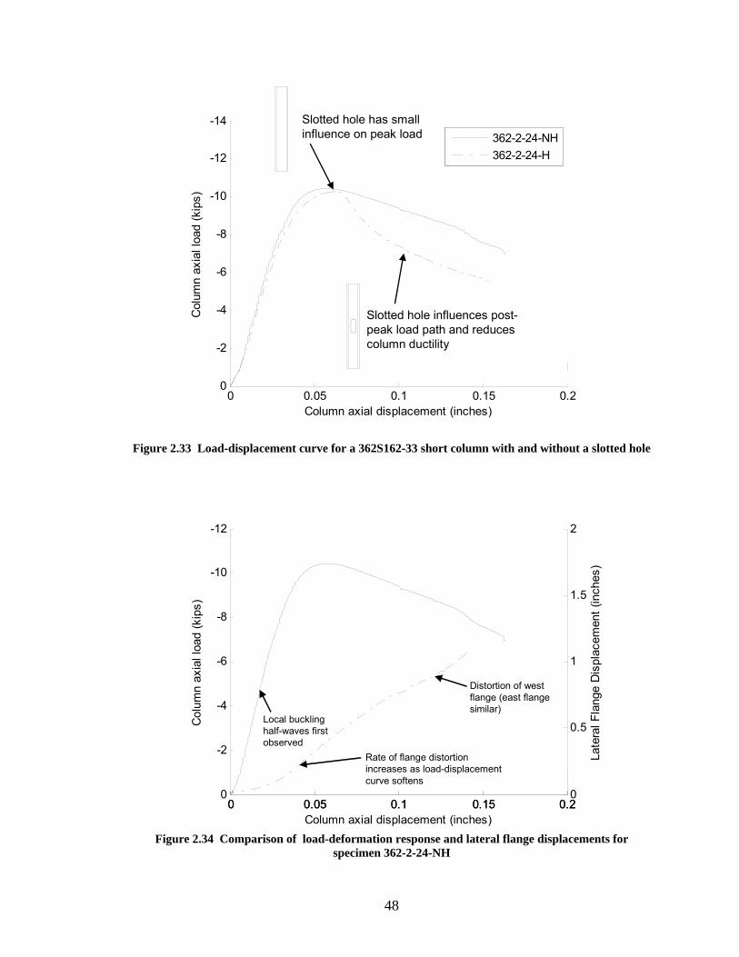
2.5.2.1 Short columns

The loading progression for the 362162S-33 short columns is depicted in

Figure 2.31 (without a hole) and Figure 2.32 (with a hole). Both columns exhibit

local buckling of the web near the supports combining with one distortional half-

wave along the length. For the column with the hole, localized hole deformation

(Figure 2.32, rightmost picture) initiates at a load of approximately 0.4Ptest and

increases in magnitude as the test progresses. The inward flange deformation

concentrates at the hole after peak load. It is hypothesized that the slotted hole

reduces the post-peak resistance of the web, forcing the flanges and lips to carry

more of the column load. This reduction in post peak resistance can be

quantified by observing the reduction in area under the load-displacement curve

for the column with the slotted hole in Figure 2.33.

47

Peak Load

Figure 2.31 Load-displacement progression for short column specimen 362-2-24-NH

Peak Load

Figure 2.32 Load-displacement progression for short column specimen 362-2-24-H

48

0 0.2 0.4 0.6 0.8 10

0.2

0.4

0.6

0.8

1

0 0.05 0.1 0.15 0.2

-14

-12

-10

-8

-6

-4

-2

0

Column axial displacement (inches)

Col

umn

axia

l loa

d (k

ips)

362-2-24-NH362-2-24-H

Slotted hole has small influence on peak load

Slotted hole influences post-peak load path and reduces column ductility

Figure 2.33 Load-displacement curve for a 362S162-33 short column with and without a slotted hole

0 0.2 0.4 0.6 0.8 10

0.2

0.4

0.6

0.8

1

0 0.05 0.1 0.15 0.2

-12

-10

-8

-6

-4

-2

0

Col

umn

axia

l loa

d (k

ips)

0 0.05 0.1 0.15 0.20

0.5

1

1.5

2

Column axial displacement (inches)

Late

ral F

lang

e D

ispl

acem

ent (

inch

es)

Distortion of west flange (east flange similar)

Local buckling half-waves first observed

Rate of flange distortion increases as load-displacement curve softens

Figure 2.34 Comparison of load-deformation response and lateral flange displacements for

specimen 362-2-24-NH

49

The position transducers at the mid-height of the short column specimens

capture the rate of lateral flange displacement associated with distortional

buckling. Figure 2.34 demonstrates that the initiation of web local buckling does

not influence the axial stiffness of specimen 362-2-24-NH, but that a softening of

the load-deformation curve coincides with the increased rate of lateral flange

movement. This observation suggests that the column deformation associated

with distortional buckling plays a larger role than local buckling in the peak load

response of the short columns. The influence of the slotted hole on the lateral

flange displacement is demonstrated in Figure 2.35, where the post-peak flange

displacement rates are observed to be higher for the 362S162-33 short column

with holes. Lateral flange displacements plots for all specimens are provided in

Appendix A.

50

0 0.2 0.4 0.6 0.8 10

0.2

0.4

0.6

0.8

1

0 0.02 0.04 0.06 0.08 0.1 0.12 0.14 0.16 0.18 0.2-1.5

-1

-0.5

0

0.5

1

1.5

Column axial displacement (inches)

Flan

ge d

ispl

acem

ent (

inch

es)

362-2-24-NH West Flange362-2-24-H West Flange

Increased rate of flange distortion is observed for column with a hole after the peak load is reached

Peak load occurs here

Figure 2.35 Influence of a slotted hole on 362S162-33 short column lateral flange displacement

Figure 2.36 and Figure 2.37 show the deformation response of the

600S162-33 short columns with and without a slotted hole. In both cases, local

buckling at the loaded ends combines with one distortional half-wave along the

column length. The deformation response of the member with and without the

hole is similar through the test progression, suggesting that the hole has a small

influence on compressive strength and post-peak ductility for the hhole/H

considered here. Figure 2.38 confirms that the slotted hole has little effect on the

post-peak load response of the column.

51

Peak Load

Figure 2.36 Load-displacement progression for short column specimen 600-1-24-NH

Peak Load

Figure 2.37 Load-displacement progression for short column specimen 600-1-24-H

52

0 0.2 0.4 0.6 0.8 10

0.2

0.4

0.6

0.8

1

0 0.05 0.1 0.15 0.2

-14

-12

-10

-8

-6

-4

-2

0

Column axial displacement (inches)

Col

umn

axia

l loa

d (k

ips)

600-1-24-NH600-1-24-H

Slotted hole has small influence on post-peak response and ductility

Figure 2.38 Load-displacement curve for a 600S162-33 short column with and without a slotted hole

2.5.2.2 Intermediate length columns

Figure 2.39 and Figure 2.40 summarize the deformation response of the

362S162-33 intermediate length columns with and without holes. In both cases,

local web buckling is first observed at approximately 0.45Ptest. The local buckling

half-waves are dampened in the vicinity of the holes. Three distortional buckling

half-waves become well-formed at approximately 0.70Ptest, overcoming the local

half-waves in the web except at the midline of the column. Note that at the peak

load three distinct local buckling half-waves are present at the midlength of the

member without the hole, while only two are present in the member with the

hole. All of the 362S162-33 intermediate length columns failed soon after the

53

peak load with a sudden loss in load-carrying capacity caused by global-

torsional buckling. Yielding of the column flanges reduces the torsional stiffness

of the section, and the friction end conditions could not restrain the twisting of

the column. The twisting of the specimen at mid-height is described by the mid-

height flange displacements in Figure 2.42.

Peak Load

Figure 2.39 Load-displacement progression for intermediate length column specimen 362-3-48-NH

54

Peak Load

Figure 2.40 Load-displacement progression for intermediate length column specimen 362-3-48-H

0 0.2 0.4 0.6 0.8 10

0.2

0.4

0.6

0.8

1

0 0.05 0.1 0.15 0.2

-14

-12

-10

-8

-6

-4

-2

0

Column axial displacement (inches)

Col

umn

axia

l loa

d (k

ips)

362-3-48-NH362-3-48-H

Columns fail abruptly with a global torsional buckling mode

Figure 2.41 Load-displacement curve for a 362S162-33 intermediate column with/ without a hole

55

0 0.2 0.4 0.6 0.8 10

0.2

0.4

0.6

0.8

1

0 0.02 0.04 0.06 0.08 0.1 0.12 0.14 0.16 0.18 0.2-1.5

-1

-0.5

0

0.5

1

1.5

Column axial displacement (inches)

Flan

ge d

ispl

acem

ent (

inch

es)

362-3-48-NH West Flange362-3-48-NH East Flange

opposite west and east flange displacement occur as the column experiences a sudden global torsional failure mode

Twisting direction

Figure 2.42 362S162-33 long column mid-height flange displacements show the global torsional

failure mode

The load-displacement response for the intermediate length 600S162-33

columns with and without slotted holes is depicted in Figure 2.43 and Figure

2.44. Local buckling is observed at approximately 0.45Ptest for both sections. The

hole does not dampen the local buckling half-wave as was the case in the

362S162-33 intermediate length column. Three distortional half-waves form as

the columns approach peak load. Two loud sounds resonate from the column

near peak load as the local web buckling half-waves at the two column ends snap

into one distortional half-wave per end. The change from local dominated to

distortional dominated web buckling is reflected as two drops near peak load for

the column without holes in Figure 2.45. The column with slotted holes is not

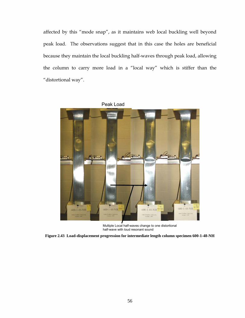
56

affected by this “mode snap”, as it maintains web local buckling well beyond

peak load. The observations suggest that in this case the holes are beneficial

because they maintain the local buckling half-waves through peak load, allowing

the column to carry more load in a “local way” which is stiffer than the

“distortional way”.

Peak Load

Multiple Local half-waves change to one distortional half-wave with loud resonant sound

Figure 2.43 Load-displacement progression for intermediate length column specimen 600-1-48-NH

57

Peak Load

Figure 2.44 Load-displacement progression for intermediate length column specimen 600-1-48-H

0 0.2 0.4 0.6 0.8 10

0.2

0.4

0.6

0.8

1

0 0.05 0.1 0.15 0.2

-14

-12

-10

-8

-6

-4

-2

0

Column axial displacement (inches)

Col

umn

axia

l loa

d (k

ips)

600-1-48-NH600-1-48-H

Drops in load occur when multiple L half-waves change abruptly to one D half-wave (north end first, then south end)

Figure 2.45 Load-displacement curve for a 600S162-33 intermediate column with/ without a hole

58

2.5.2.3 Comments on the Friction-Bearing End Conditions

There are advantages and disadvantages to the friction-bearing end

conditions used in these column tests. One obvious advantage is that the

specimen alignment and preparation can be performed without welding or the

use of grout or hydrostone. The heat from welding can influence the material

properties of the steel in the column. The use of grout or hydrostone does not

guarantee a flat bearing surface, and the bearing surfaces cannot be inspected

because they are hidden from view. Restraining the column ends with welds or

grout is not common in practice and may produce specimen strengths that are

unconservative when compared to field conditions. Friction bearing specimens

can be aligned by hand in the testing machine without special equipment.

The primary disadvantage of the friction-bearing end conditions is that the

test results hinge on the flatness of the compression platens and of the specimen

ends. Great care and time is required to prepare the specimen ends, and small

deviations in flatness can significantly impact the tested results and failure

modes. Finite element modeling in the post-peak range of specimens with these

end conditions is also difficult because the interaction between the column and

the platen is complicated.

It is concluded from the experiences in this study that the friction-bearing

end conditions can be used to study local and distortional type failures of short

and long columns, although they may not be satisfactory for all types of global

buckling failures. Local web buckling was uninhibited but distortional buckling

59

was restrained at the column ends by the one-way compression warping fixity.

Friction between the column ends and the platens prevented a change in shape

of the cross section up to peak load, but slipping of the cross section was

observed after peak load. This slipping was signaled by loud metal- on- metal

“popping” sounds associated with observable changes in the cross section

(usually flaring of the flanges) at the column ends. Also, uplift warping

deformations (Figure 2.46) occurred in the post-peak range for some columns

experiencing distortional type failures. The long 362S162-33 columns

experienced a sudden global-torsional failure shortly after reaching the peak load

as the twisting of the columns overcame the friction between the column ends

and the platens. In this case, the friction-bearing end conditions did not allow a

detailed study of the global-torsional post-peak response.

Flange-lip corner lifts off platen when large deformations exist past peak load

Figure 2.46 Column specimen flange-lip corner lifts off platen during post-peak portion of test

60

2.6 Conclusions

An experimental study was conducted to evaluate the influence of

industry-standard slotted holes on short and intermediate length cold-formed

steel structural studs. The presences of slotted holes caused only slight decreases

in the ultimate compressive strength of the columns, although the post-peak

response and column ductility were influenced by the addition of holes in most

cases. The influence on post-peak response is observed to be related to the way

that the holes influence the local and distortional buckling behavior of the

columns under load. In the case of the 362S162-33 short and intermediate length

columns, the slotted holes reduced the web local buckling capacity, causing the

column to rely more on the flanges and lip stiffeners to carry load. The slotted

holes retained local buckling behavior in the 600S162-33 at peak load, providing

a small boost in strength and ductility of the column. The post-peak response of

the 600S162-33 short columns was not influenced by the presence of the slotted

holes.

2.7 Future Work

In the short term, these column test results will be used to calibrate

nonlinear finite element models of cold-formed steel compression members with

holes. The time and effort required to test specimens in the laboratory is

tremendous, and therefore having a reliable computational platform to evaluate

the influence of holes in a parametric way is essential to extending the Direct

61

Strength Method to members with holes. The test results will also be compared

to DSM style strength predictions employing the elastic buckling behavior of the

individual specimens.

Additional experimental work is required to provide more strength data

points on columns with varying hole sizes, shapes, and spacings. Also, tests with

boundary conditions consistent with those used in practice are also needed.

From a general industry perspective, simplified methods for predicting ductility

could be useful when designing and detailing cold-formed steel members,

particularly for seismic applications. These methods may employ basic

mechanics and yield-line theory in combination with elastic buckling mode

shapes to approximate a cold-formed steel member’s post-peak response and

energy absorption capacity.

3 Predicting the Ultimate Strength of Cold-Formed Steel Beams with Holes using a DSM Approach

3.1 Introduction

The Direct Strength Method (DSM) relies on critical elastic buckling loads

to predict the strength of cold-formed steel members. Therefore, to develop a

reliable DSM approach for cold-formed steel beams with holes requires a

fundamental understanding of how perforations influence elastic buckling

behavior. In this study, the elastic buckling properties of 72 cold-formed steel

beam specimens are evaluated, paying close attention to unique buckling modes

62

created by holes in the beam webs. The elastic buckling information is used to

produce DSM flexural strength predictions which are then compared to the

tested specimen results.

3.2 Beam Specimen Dimensions and Tested Conditions

The beam experiments considered in this study were conducted by Shan,

LaBoube, Schuster, and Batson in the early nineties and consist of three separate

test sequences (Batson 1992, Shan and LaBoube 1994, Schuster 1992). Test

Sequences 1 and 2 were performed at the University of Missouri-Rolla (UMR)

and Test Sequence 3 at the University of Waterloo. Each specimen is made up of

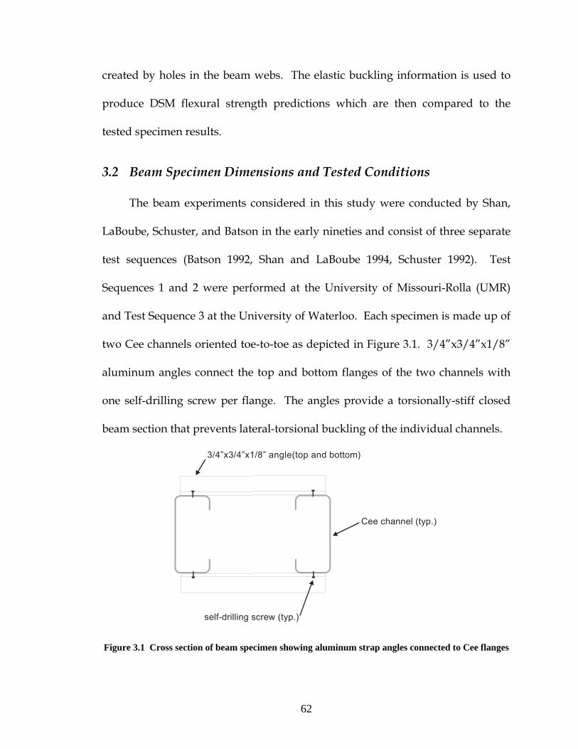
two Cee channels oriented toe-to-toe as depicted in Figure 3.1. 3/4”x3/4”x1/8”

aluminum angles connect the top and bottom flanges of the two channels with

one self-drilling screw per flange. The angles provide a torsionally-stiff closed

beam section that prevents lateral-torsional buckling of the individual channels.

3/4”x3/4”x1/8” angle(top and bottom)

self-drilling screw (typ.)

Cee channel (typ.)

Figure 3.1 Cross section of beam specimen showing aluminum strap angles connected to Cee flanges

63

Beam cross section dimension nomenclature is presented in Figure 3.2 and the

measured dimensions are summarized in Table 3.1. The Cee channel inside

corner radii are assumed as twice the measured thickness of the specimen. The

steel yield stress for each specimen, fy, is provided in Table 3.1 and varies from

22.0 ksi to 93.3 ksi with a mean of 48.6 ksi. This extremely large variation in yield

stress was somewhat unexpected.

Two hole shapes are considered in the study, an industry standard slotted

hole and a tri-slotted hole with the curved hole ends replaced by triangular tips.

The holes are centered in the web and are mechanically punched at 24 inches on

center longitudinally with a hole at the center of the span. Hole dimension

nomenclature is presented in Figure 3.2.

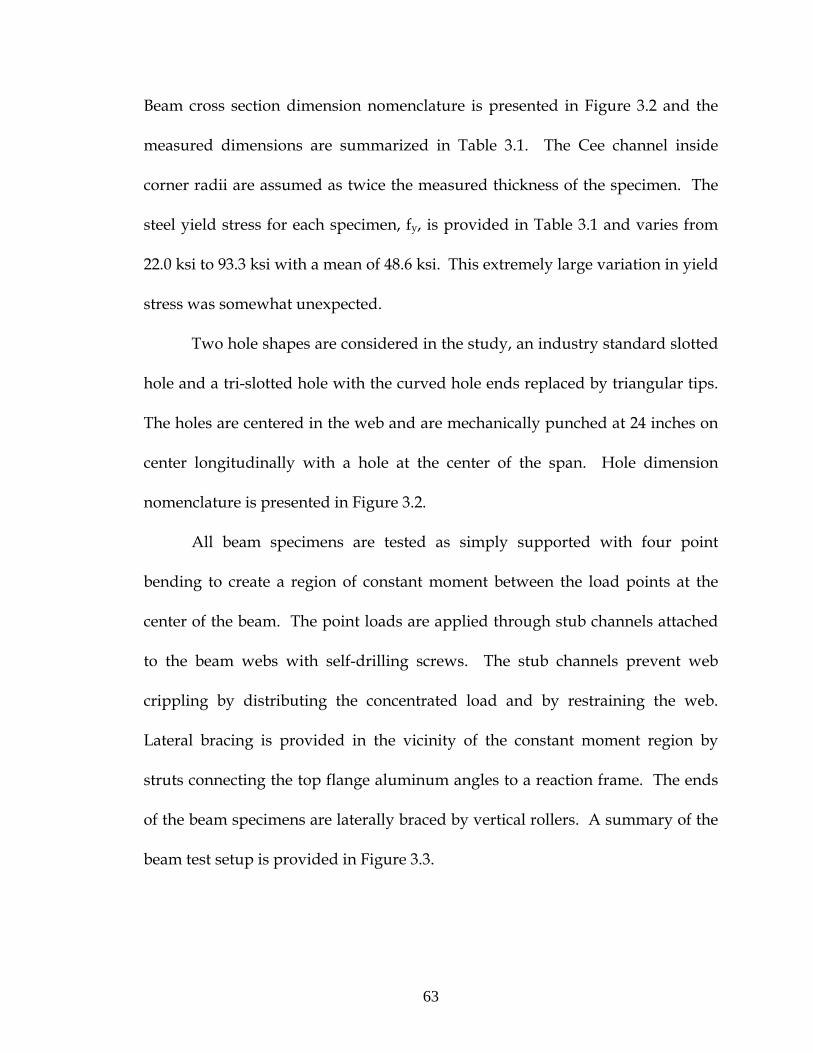
All beam specimens are tested as simply supported with four point

bending to create a region of constant moment between the load points at the

center of the beam. The point loads are applied through stub channels attached

to the beam webs with self-drilling screws. The stub channels prevent web

crippling by distributing the concentrated load and by restraining the web.

Lateral bracing is provided in the vicinity of the constant moment region by

struts connecting the top flange aluminum angles to a reaction frame. The ends

of the beam specimens are laterally braced by vertical rollers. A summary of the

beam test setup is provided in Figure 3.3.

64

Slotted Hole

Tri-slotted Hole

Lhole

hhole

0.5*hhole

Rhole

B21

H2

RD21

tH1

D12

B22

D22

B11

B12

6”

D11

Channel 1 Channel 2

Figure 3.2 Channel cross section and web hole nomenclature

Table 3.1 Beam cross section dimensions and material properties

Steel Yield

Stress

L X Hole Type h hole L hole R hole H 1 H 2 B 11 B 21 B 12 B 22 D 11 D 21 D 12 D 22 R t Fyin. in. in. in. in. in. in. in. in. in. in. in. in. in. in. in. in. ksi

1 2,16,1&2(H) 150.0 39.0 Slotted 0.750 2.000 0.375 2.510 2.510 1.610 1.610 1.630 1.610 0.400 0.450 0.420 0.430 0.124 0.062 37.21 2,20,1&2(H) 150.0 39.0 Slotted 0.750 2.000 0.375 2.500 2.480 1.600 1.600 1.600 1.600 0.420 0.410 0.420 0.410 0.078 0.039 33.71 2,20,3,4(H) 150.0 39.0 Slotted 0.750 2.000 0.375 2.510 2.520 1.590 1.620 1.580 1.600 0.360 0.420 0.470 0.410 0.078 0.039 33.71 3,14,1&2(H) 150.0 39.0 Slotted 1.500 4.000 0.750 3.680 3.680 1.650 1.640 1.630 1.630 0.570 0.550 0.560 0.520 0.154 0.077 63.71 3,14,3&4(H) 150.0 39.0 Slotted 1.500 4.000 0.750 3.690 3.690 1.630 1.620 1.640 1.630 0.530 0.530 0.620 0.550 0.154 0.077 63.71 3,18,1&2(H) 150.0 39.0 Slotted 1.500 4.000 0.750 3.750 3.650 1.560 1.560 1.570 1.580 0.580 0.560 0.580 0.540 0.088 0.044 46.91 3,18,3&4(H) 150.0 39.0 Slotted 1.500 4.000 0.750 3.650 3.640 1.560 1.580 1.560 1.570 0.560 0.570 0.540 0.540 0.088 0.044 46.91 3,20,1&2(H) 150.0 39.0 Slotted 1.500 4.000 0.750 3.650 3.710 1.560 1.640 1.550 1.590 0.520 0.560 0.550 0.560 0.088 0.044 46.81 3,20,3&4(H) 150.0 39.0 Slotted 1.500 4.000 0.750 3.670 3.690 1.560 1.590 1.550 1.610 0.600 0.560 0.520 0.590 0.088 0.044 46.81 12,14,1&2(H) 192.0 60.0 Slotted 1.500 4.000 0.750 12.080 12.070 1.640 1.630 1.690 1.630 0.690 0.600 0.600 0.620 0.196 0.098 35.91 12,14,3&4(H) 192.0 60.0 Slotted 1.500 4.000 0.750 12.050 12.000 1.640 1.600 1.670 1.710 0.650 0.640 0.650 0.640 0.196 0.098 35.91 12,16,1&2(H) 192.0 60.0 Slotted 1.500 4.000 0.750 11.960 11.970 1.570 1.570 1.570 1.560 0.500 0.610 0.520 0.430 0.110 0.055 49.11 12,16,3&4(H) 192.0 60.0 Slotted 1.500 4.000 0.750 12.070 11.960 1.560 1.570 1.570 1.580 0.420 0.530 0.580 0.530 0.110 0.055 49.12 2B,16,1&2(H) 150.0 39.0 Slotted 1.500 4.000 0.750 2.460 2.460 1.620 1.630 1.620 1.610 0.470 0.460 0.510 0.510 0.118 0.059 53.62 2B,16,3&4(H) 150.0 39.0 Slotted 1.500 4.000 0.750 2.470 2.460 1.630 1.620 1.620 1.630 0.470 0.520 0.520 0.460 0.118 0.059 53.62 2B,20,1&2(H) 150.0 39.0 Slotted 1.500 4.000 0.750 2.420 2.420 1.630 1.640 1.630 1.620 0.420 0.420 0.500 0.500 0.066 0.033 67.22 2B,20,3&4(H) 150.0 39.0 Slotted 1.500 4.000 0.750 2.420 2.430 1.630 1.640 1.630 1.620 0.420 0.410 0.500 0.500 0.066 0.033 67.22 3B,14,1&2(H) 150.0 39.0 Slotted 1.500 4.000 0.750 3.650 3.620 1.620 1.660 1.630 1.630 0.540 0.550 0.490 0.500 0.142 0.071 81.42 3B,14,3&4(H) 150.0 39.0 Slotted 1.500 4.000 0.750 3.640 3.630 1.630 1.620 1.620 1.630 0.540 0.470 0.490 0.540 0.142 0.071 81.42 3B,18,1&2(H) 150.0 39.0 Slotted 1.500 4.000 0.750 3.610 3.630 1.610 1.650 1.650 1.620 0.510 0.520 0.500 0.500 0.088 0.044 53.12 3B,18,3&4(H) 150.0 39.0 Slotted 1.500 4.000 0.750 3.620 3.630 1.620 1.660 1.650 1.640 0.500 0.500 0.520 0.520 0.088 0.044 53.12 3B,20,1&2(H) 150.0 39.0 Slotted 1.500 4.000 0.750 3.610 3.600 1.630 1.620 1.630 1.620 0.460 0.470 0.460 0.470 0.072 0.036 63.72 3B,20,3&4(H) 150.0 39.0 Slotted 1.500 4.000 0.750 3.610 3.610 1.640 1.630 1.640 1.630 0.460 0.470 0.470 0.470 0.072 0.036 63.72 3B,20,5&6(H) 150.0 39.0 Slotted 1.500 4.000 0.750 3.600 3.600 1.630 1.630 1.620 1.630 0.460 0.460 0.460 0.470 0.072 0.036 63.72 3B,20,1&2(T) 150.0 39.0 Tri-slotted 1.500 4.500 --- 3.560 3.570 1.620 1.650 1.680 1.600 0.590 0.640 0.620 0.610 0.058 0.029 25.52 3B,20,3&4(T) 150.0 39.0 Tri-slotted 1.500 4.500 --- 3.560 3.560 1.620 1.680 1.690 1.610 0.580 0.630 0.620 0.570 0.058 0.029 25.52 6B,18,1&2(H) 192.0 60.0 Slotted 1.500 4.000 0.750 6.060 6.050 1.620 1.620 1.550 1.550 0.470 0.470 0.500 0.500 0.092 0.046 47.22 6B,18,3&4(H) 192.0 60.0 Slotted 1.500 4.000 0.750 6.050 6.020 1.620 1.620 1.550 1.550 0.470 0.480 0.500 0.510 0.092 0.046 47.22 6C,18,1&2(H) 192.0 60.0 Slotted 1.500 4.000 0.750 5.960 5.960 1.980 1.990 1.980 1.990 0.640 0.590 0.590 0.640 0.096 0.048 75.12 6C,18,3&4(H) 192.0 60.0 Slotted 1.500 4.000 0.750 5.950 5.980 1.970 1.980 1.990 1.980 0.600 0.650 0.640 0.630 0.096 0.048 75.12 6D,18,1&2(H) 192.0 60.0 Slotted 1.500 4.000 0.750 6.020 6.020 2.420 2.430 2.430 2.430 0.700 0.620 0.620 0.700 0.092 0.046 30.82 6D,18,3&4(H) 192.0 60.0 Slotted 1.500 4.000 0.750 6.020 6.020 2.430 2.430 2.430 2.430 0.700 0.700 0.610 0.620 0.092 0.046 30.82 6B,20,1&2(H) 192.0 60.0 Slotted 1.500 4.000 0.750 5.920 5.920 1.630 1.620 1.520 1.530 0.440 0.470 0.440 0.420 0.066 0.033 93.32 8A,14,1&2(H) 192.0 60.0 Slotted 1.500 4.000 0.750 8.060 8.060 1.380 1.380 1.380 1.380 0.490 0.480 0.410 0.430 0.148 0.074 31.02 8A,14,3&4(H) 192.0 60.0 Slotted 1.500 4.000 0.750 8.070 8.070 1.380 1.380 1.380 1.380 0.500 0.410 0.410 0.500 0.148 0.074 31.02 8A,14,5&6(H) 192.0 60.0 Slotted 1.500 4.000 0.750 8.070 8.070 1.370 1.380 1.380 1.370 0.410 0.500 0.490 0.410 0.148 0.074 31.02 8A,14,7&8(H) 192.0 60.0 Slotted 1.500 4.000 0.750 8.030 8.030 1.390 1.390 1.390 1.400 0.430 0.480 0.480 0.450 0.130 0.065 56.32 8A,14,9&10(H) 192.0 60.0 Slotted 1.500 4.000 0.750 8.040 8.040 1.390 1.380 1.380 1.380 0.460 0.440 0.450 0.480 0.130 0.065 56.32 8B,14,1&2(T) 192.0 60.0 Tri-slotted 1.500 4.500 --- 8.050 8.050 1.640 1.630 1.640 1.640 0.630 0.640 0.670 0.660 0.134 0.067 32.62 8B,14,3&4(T) 192.0 60.0 Tri-slotted 1.500 4.500 --- 8.050 8.040 1.640 1.640 1.640 1.640 0.640 0.640 0.660 0.650 0.134 0.067 32.62 8B,14,5&6(T) 192.0 60.0 Tri-slotted 1.500 4.500 --- 8.020 8.020 1.630 1.640 1.640 1.630 0.640 0.630 0.640 0.630 0.130 0.065 53.12 8B,14,7&8(T) 192.0 60.0 Tri-slotted 1.500 4.500 --- 8.030 8.030 1.630 1.630 1.630 1.630 0.660 0.610 0.610 0.660 0.130 0.065 53.12 8D,14,1&2(T) 192.0 60.0 Tri-slotted 1.500 4.500 --- 7.950 7.960 2.480 2.500 2.470 2.490 0.640 0.480 0.470 0.620 0.130 0.065 54.72 8D,14,3&4(T) 192.0 60.0 Tri-slotted 1.500 4.500 --- 7.950 7.950 2.470 2.490 2.470 2.480 0.660 0.480 0.450 0.610 0.130 0.065 54.72 8B,18,1&2(H) 192.0 60.0 Slotted 1.500 4.000 0.750 7.950 7.940 1.590 1.580 1.580 1.580 0.470 0.470 0.480 0.470 0.090 0.045 72.32 8D,18,1&2(H) 192.0 60.0 Slotted 1.500 4.000 0.750 8.000 8.000 2.420 2.450 2.440 2.430 0.610 0.690 0.690 0.620 0.092 0.046 22.02 8D,18,3&4(H) 192.0 60.0 Slotted 1.500 4.000 0.750 8.000 8.000 2.420 2.450 2.450 2.430 0.600 0.700 0.700 0.600 0.092 0.046 22.02 8A,20,1&2(H) 192.0 60.0 Slotted 1.500 4.000 0.750 7.930 7.930 1.380 1.390 1.380 1.380 0.410 0.440 0.450 0.430 0.062 0.031 38.02 8A,20,3&4(H) 192.0 60.0 Slotted 1.500 4.000 0.750 7.930 7.920 1.370 1.380 1.390 1.370 0.450 0.430 0.430 0.440 0.062 0.031 38.02 8B,20,1&2(T) 192.0 60.0 Tri-slotted 1.500 4.500 --- 7.970 7.970 1.630 1.640 1.630 1.620 0.610 0.610 0.600 0.620 0.062 0.031 44.92 8B,20,3&4(T) 192.0 60.0 Tri-slotted 1.500 4.500 --- 7.960 7.960 1.630 1.630 1.620 1.630 0.620 0.580 0.580 0.620 0.062 0.031 44.92 8B,20,5&6(T) 192.0 60.0 Tri-slotted 1.500 4.500 --- 7.950 7.950 1.630 1.630 1.630 1.630 0.610 0.600 0.600 0.610 0.062 0.031 44.92 8B,20,7&8(T) 192.0 60.0 Tri-slotted 1.500 4.500 --- 7.950 7.950 1.630 1.630 1.640 1.630 0.610 0.620 0.610 0.620 0.062 0.031 44.92 8D,20,1&2(T) 192.0 60.0 Tri-slotted 1.500 4.500 --- 7.940 7.940 2.490 2.450 2.450 2.490 0.640 0.590 0.590 0.640 0.086 0.043 38.62 8D,20,3&4(T) 192.0 60.0 Tri-slotted 1.500 4.500 --- 7.940 7.940 2.460 2.460 2.440 2.480 0.640 0.590 0.590 0.650 0.086 0.043 38.62 8D,20,5&6(T) 192.0 60.0 Tri-slotted 1.500 4.500 --- 7.950 7.950 2.490 2.460 2.450 2.480 0.620 0.620 0.620 0.630 0.086 0.043 38.62 12B,16,1&2(H) 192.0 60.0 Slotted 1.500 4.000 0.750 11.950 11.950 1.630 1.630 1.630 1.630 0.530 0.540 0.520 0.530 0.120 0.060 60.62 12B,16,3&4(H) 192.0 60.0 Slotted 1.500 4.000 0.750 11.980 12.020 1.630 1.630 1.620 1.630 0.470 0.500 0.550 0.530 0.120 0.060 60.62 12B,16,5&6(H) 192.0 60.0 Slotted 1.500 4.000 0.750 11.960 11.970 1.630 1.630 1.630 1.630 0.510 0.500 0.510 0.520 0.120 0.060 60.62 12B,16,7&8(H) 192.0 60.0 Slotted 1.500 4.000 0.750 11.970 11.960 1.630 1.630 1.620 1.630 0.480 0.550 0.560 0.490 0.120 0.060 60.63 BP4—40(H) 168.0 48.0 Slotted 1.5 4.02 0.750 7.99 7.99 1.61 1.61 1.61 1.61 0.47 0.47 0.47 0.47 0.094 0.047 38.93 BP5—40(H) 168.0 48.0 Slotted 1.5 4.02 0.750 7.99 7.99 1.61 1.61 1.61 1.61 0.47 0.47 0.47 0.47 0.094 0.047 38.93 BP6—40(H) 168.0 48.0 Slotted 1.5 4.02 0.750 7.99 7.99 1.61 1.61 1.61 1.61 0.47 0.47 0.47 0.47 0.094 0.047 38.93 BP7—65(H) 168.0 48.0 Slotted 2.48 4.53 0.750 7.99 7.99 1.58 1.58 1.58 1.58 0.47 0.47 0.47 0.47 0.094 0.047 38.93 BP8—65(H) 168.0 48.0 Slotted 2.48 4.53 0.750 7.99 7.99 1.61 1.58 1.61 1.58 0.47 0.47 0.47 0.47 0.094 0.047 38.93 BP9—65(H) 168.0 48.0 Slotted 2.48 4.53 0.750 7.99 7.99 1.61 1.58 1.58 1.58 0.47 0.47 0.47 0.47 0.094 0.047 49.03 CP4—40(T) 168.0 48.0 Tri-slotted 1.69 4.65 --- 7.99 7.99 1.58 1.58 1.58 1.58 0.51 0.51 0.51 0.51 0.096 0.048 49.03 CP5—40(T) 168.0 48.0 Tri-slotted 1.69 4.65 --- 7.99 7.99 1.58 1.61 1.58 1.58 0.51 0.51 0.51 0.51 0.096 0.048 49.03 CP6—40(T) 168.0 48.0 Tri-slotted 1.69 4.65 --- 8.03 8.03 1.61 1.61 1.58 1.58 0.53 0.51 0.51 0.51 0.096 0.048 49.03 CP7—65(T) 168.0 48.0 Tri-slotted 2.52 4.61 --- 7.99 7.99 1.61 1.61 1.61 1.61 0.51 0.51 0.51 0.51 0.096 0.048 49.03 CP8—65(T) 168.0 48.0 Tri-slotted 2.52 4.61 --- 8.03 7.99 1.58 1.61 1.58 1.61 0.51 0.51 0.51 0.53 0.096 0.048 49.03 CP9—65(T) 168.0 48.0 Tri-slotted 2.52 4.61 --- 7.99 7.99 1.61 1.61 1.63 1.61 0.53 0.51 0.51 0.51 0.096 0.048 49.0

Cross Section Dimensions

Test Sequence

Specimen Name Member Length,

Load Location Hole Dimensions

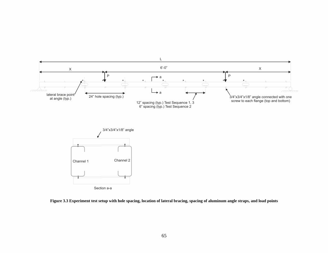
65

X

L

X

P P

12” spacing (typ.) Test Sequence 1, 36” spacing (typ.) Test Sequence 2

3/4”x3/4”x1/8” angle connected with one screw to each flange (top and bottom)

6’-0”

a

a

24” hole spacing (typ.)

Section a-a

3/4”x3/4”x1/8” angle

Channel 1 Channel 2

** * * * * * * *

lateral brace point at angle (typ.)

Figure 3.3 Experiment test setup with hole spacing, location of lateral bracing, spacing of aluminum angle straps, and load points

66

3.3 Finite Element Modeling

The elastic buckling behavior of the 72 beam specimens is obtained with

eigenbuckling analyses in ABAQUS (ABAQUS 2004). All beams are modeled

with S9R5 reduced integration nine-node thin shell elements. Refer to Progress

Report #1 for a detailed discussion of the S9R5 element (Moen and Schafer 2006).

Cold-formed steel material properties are assumed as E=29500 ksi and ν=0.3.

The centerline Cee channel cross section dimensions used in ABAQUS are

calculated from the out-to-out dimensions in Table 3.1.

Beam end restrained in 2 and 3 (v, w=0)

Beam end restrained in 2 and 3 (v, w=0)

Bottom flange restrained in 1 at support (u=0)

* **

**

**

**

Restrain node at midline of top flange in 3 (w=0) (Typ.)

Rigid body connection between top (and bottom) flange midline nodes (Typ.)

Figure 3.4 Finite element model boundary conditions for eigenbuckling analyses

Special care is taken to simulate the experimental boundary conditions

when modeling in ABAQUS. The simple supports with vertical roller restraints,

the aluminum angle straps connecting the top and bottom channel flanges, the

lateral bracing of the top flange in the constant moment region, and the

application of load through the webs and are all considered. Figure 3.4

summarizes the ABAQUS boundary condition assumptions.

67

To simulate the simply supported conditions with vertical rollers, the ends

of the beams are modeled as warping free except for the bottom flange at one

end which is restrained to prevent longitudinal rigid body movement. The

channel cross sections are restrained from vertical and lateral translation at both

beam ends.

A rigid body restraint is used to model the connectivity between the top

and bottom Cee channel flanges provided by the aluminum angle straps

connected with self-drilling screws. In Figure 3.5 each angle is modeled as a

rigid body made up of one midline flange node from each channel. The rigid

body definition requires that the motion (both translational and rotational) of the

two nodes is governed by a single reference node, in this case the midline flange

node of Channel 1. The formulation allows for rigid body motion but requires

that the relative position of the two nodes remain constant. A disadvantage of

this rigid body restraint is that flange movements are only restrained at the

midline node. This simplification sometimes results in distortional buckling

modes that are not physically possible due to the one way (in this case upward)

contact interaction between the angle strap and the flange.

68

1 inch mesh spacing (typ.)

Rigid body connection between top (and bottom) flange midline nodes

Rigid body reference node

Channel 1

Channel 2 Figure 3.5 Channel and hole meshing details and modeling of aluminum angle straps

Element meshing is performed with a custom-built Matlab program

(Mathworks 2006) written by the author. Figure 3.5 provides an example of a

typical beam mesh where the longitudinal mesh spacing is one inch and holes

are defined with a series of element lines radiating from the opening. Figure 3.6

provides a close-up view of the rounded corner meshing of the channels. Two

elements model the rounded corners here because S9R5 elements have quadratic

shape functions which allow the initial curved geometry. Refer to Section 3.3 of

Progress Report #1 for more information on modeling rounded corners with

S9R5 elements (Moen and Schafer 2006). The maximum corner element aspect

ratio is limited in all finite element models to 16:1. The typical element aspect

ratio in the flat portions of each specimen is 1:1.

69

2-ABAQUS S9R5 finite elements used for rounded corners of channels (max element aspect ratio of 16 to 1)

Figure 3.6 ABAQUS meshing details for Cee channel rounded corners

Concentrated loads are applied to the beam specimens through vertical

stub channels connected to the beam webs with self-drilling screws. To simulate

the distribution of the load into a channel web, the concentrated load is applied

as a group of web point loads in ABAQUS. Figure 3.7 demonstrates how the

concentrated loads are applied to the beam webs in the finite element models. It

should be noted that the web local buckling restraint provided by the stub

channels is not modeled in ABAQUS because it was observed to have a

negligible influence on the elastic buckling behavior in the relatively long

constant moment regions of the beams.

70

The transfer of load from the stub channels through the self-drilling screws is simulated as a series of web point loads in ABAQUS

Stub channel

Applied load

Figure 3.7 Modeling of the beam concentrated loads in ABAQUS

3.4 Elastic Buckling Results

The beam specimen elastic buckling modes are reviewed one-by-one in

ABAQUS by the author to identify the pure local (L) and distortional (D)

buckling modes as well as any mixed elastic modes created by the addition of

web holes. Lateral-torsional buckling is restrained by the top flange lateral

bracing and aluminum angle straps (see Figure 3.3), although other possible

global (G) buckling modes are possible as discussed in Section 3.4.3 of this

report.

The mode identification process for beams with holes is guided by the

experiences obtained in Progress Report #1 for cold-formed steel compression

members with holes (Moen and Schafer 2006). Cee channel columns with web

holes exhibited unique mixed buckling modes where distortion of the flanges

near the hole mixes with local buckling (DH+L) at critical elastic buckling loads

less that the pure D mode. In this beam study mixed distortional modes are

71

again observed, as well as local web hole modes initiated by the compression

component of the stress gradient from bending.

3.4.1 Local Buckling

The slotted holes in the beam specimen webs created unique local

buckling modes and reduce the critical elastic local buckling moment in most

cases. The shallow beam specimen (nominal depth of 2.5 inches) in Figure 3.8(a)

exhibits local buckling in both the top flange and the web. The addition of

slotted web holes in Figure 3.8(b) creates two new local buckling modes, the LH

and LH2 modes. The LH mode is identified by the buckling of the strip of web

above the hole into a single half-wave. The influence of this buckling mode on

the ultimate strength of cold-formed steel compression members was formalized

by Miller and Peköz and is accounted for in the current Specification as the

“unstiffened strip approach” (Miller and Peköz, 1989, 1994). The LH2 mode

occurs when the strip of web above the hole buckles in two half-waves. The

critical elastic buckling moments for the LH and LH2 modes are eight percent

less than that of the pure L mode, suggesting that these local hole modes will

influence the ultimate strength of the beam. It is also noted that the LH and LH2

elastic buckling moments are the same for this member. This result is consistent

with the elastic buckling solution for an unstiffened plate in compression, which

produces essentially identical critical buckling stresses for one half-wave or

multiple half-waves (see Yu and Schafer 2006).

72

Figure 3.9 compares the elastic buckling behavior of a slightly deeper

beam (nominal depth of 3.625 inches) with and without holes. The addition of

slotted web holes in this case creates the LH2 mode with a critical elastic

buckling moment that is 17 percent less than the pure L mode. The LH mode is

not observed for this specimen, although a variant of the mode shown in Figure

3.16 is identified as a distortional hole mode (DH) for the specimen. This

classification decision highlights the difficulties in identifying local and

distortional hole modes and insinuates that these LH and DH modes are related.

Figure 2.10, Figure 2.11, and Figure 2.12 summarize the influence of

slotted holes on the local buckling behavior of deeper beams with nominal

heights of 6 inches, 8 inches, and 12 inches respectively. The LH local hole mode

consistently exhibits the lowest critical elastic buckling moment, although as

beam depth increases from 6 inches to 12 inches the difference between the LH

and pure L mode decreases from 20 percent to 5 percent for the specimens

shown.

73

No holesHoles

LMcrl/Myg=0.82

LHMcrl/Myg=0.77

LH2Mcrl/Myg=0.77

LMcrl/Myg=0.83

Figure 3.8 Local buckling modes for specimen 2B,20,1&2(H) with and without holes

No holes Holes

LMcrl/Myg=3.00

LH2Mcrl/Myg=2.49

LMcrl/Myg=3.02

Figure 3.9 Local buckling modes for specimen 3B,14,1&2(H) with and without holes

74

LMcrl/Myg=1.05

LH2Mcrl/Myg=0.87

LMcrl/Myg=1.07

LHMcrl/Myg=0.75

No holes Holes

Figure 3.10 Local buckling modes for specimen 6B,18,1&2(H) with and without holes

LMcrl/Myg=0.78

LH2Mcrl/Myg=0.72

LMcrl/Myg=0.79

LHMcrl/Myg=0.63

No holes Holes

Figure 3.11 Local buckling modes for specimen BP-40(H) with and without holes

75

LMcrl/Myg=0.96

LMcrl/Myg=0.89

LHMcrl/Myg=0.85

No holes Holes

Figure 3.12 Local buckling modes for specimen 12B,16,1&2(H) with and without holes

This relationship between critical elastic local buckling moment, Mcrl , and

the ratio of hole depth to member depth is captured in Figure 2.13. Mcrl is

defined as the minimum local buckling moment:

),2,,,2,min( 222111 CCCCCCcr LLHLHLLHLHM =l

where C1 and C2 denote the two channels that make up a beam specimen. When

hhole/H is small, Mcrl shows only a slight decrease. When hhole/H is large, the

strip of web above the hole is narrow and acts as a stiffener in the vicinity of the

hole and again the influence on Mcrl is small. Mcrl

is at a minimum when

hhole/H=0.25. A similar trend has been observed when considering the influence

76

of hole width on the critical elastic buckling stress of simply supported plates

loaded uniaxially in compression (Moen and Schafer 2006).

0 0.2 0.4 0.6 0.8 10

0.2

0.4

0.6

0.8

1

0 0.2 0.4 0.6 0.8 10

0.5

1

1.5

hhole/H

Mcr

l ,hol

e/Mcr

l ,no

hole

Figure 3.13 Influence of holes on Mcrl

The influence of experiment boundary conditions on the elastic buckling

behavior is evaluated by comparing the critical elastic buckling moment Mcrl

(without holes) from the ABAQUS eigenbuckling analyses to the buckling

moment of each channel individually determined with the finite strip software

CUFSM. Since the finite strip method considers elastic buckling of each channel

individually under a constant moment, the comparison of ABAQUS and CUFSM

results isolate the influence of the aluminum angle straps at the top and bottom

flanges, as well as the lateral bracing and the application of the constant moment

as a series of point loads in the experiments. Figure 3.14 demonstrates that the

77

experiment loading and boundary conditions have a small influence on the

critical elastic buckling moment Mcrl for the specimens considered in this study.

0 0.2 0.4 0.6 0.8 10

0.2

0.4

0.6

0.8

1

0 50 100 150 200 250 3000

0.5

1

1.5

H/t

Mcr

l ,no

hole

, ABA

QU

S/Mcr

l ,CU

FSM

Figure 3.14 Influence of test boundary conditions on Mcrl

3.4.2 Distortional Buckling The experimental boundary conditions and the slotted web holes influence the

distortional buckling behavior of the specimens in this study. The aluminum

angle straps connecting the top (compression) flange increase the rotational

stiffness of the beam flanges (See Figure 3.1). This increase in stiffness boosts the

critical elastic buckling loads for distortional buckling and modifies the half-

wavelengths from those predicted by the finite strip method. The presence of

slotted web holes also influences distortional buckling by initiating distortion of

the top flanges near the holes mixed with local buckling (DH+L). These mixed

78

modes have critical elastic buckling loads less than that of the pure distortional

(D) mode and resemble the DH+L modes in the compression members studied in

Progress Report #1.

Figure 2.15 compares the influence of slotted web holes on the distortional

buckling of a shallow beam specimen (nominal height of 2.5 inches). For the

specimen with holes, the DH+L mode is present with a critical elastic buckling

moment 20 percent less that the pure D mode. The D mode without holes

becomes a mixed distortional-local mode ( D+L) when holes are added, although

the critical elastic buckling moment is not significantly affected in this case. This

specimen is sensitive to mixing of local and distortional modes because of the

relatively thin steel sheet thickness t of 0.033 inches. It is also noted that the hole

has only a small influence on the distortional buckling half-wavelength for this

specimen.

The slightly deeper beam specimen (nominal height of 3.625 inches) in

Figure 3.16 again demonstrates the DH distortional buckling mode at the hole.

The sheet thickness for these channels is roughly double that of the previously

discussed specimen (t=0.71 inches) and the hole depth is unchanged. The critical

elastic local buckling moment is higher than the distortional buckling moment

because of the increased thickness, resulting in DH and D modes without local

buckling interaction when the slotted holes are present. The critical elastic

buckling moment of the DH mode is still 13 percent less than that of the pure D

mode, demonstrating that for a beam of this depth and steel sheet thickness,

79

elastic buckling is still influenced by the web holes. It is also noted that the

buckling of the strip of web above the hole in this DH mode into a single half-

wavelength resembles the LH mode for this same specimen discussed in Section

3.4.1. The similarities between the LH and DH modes make it difficult to

differential between these modes for this specimen. A formal modal

identification method will be the subject of future work.

No holes Holes

DMcrd/Myg=1.08Half wavelength=13 inches

DH+LMcrd/Myg=0.83

D+LMcrd/Myg=1.03Half wavelength=14 inches

Figure 3.15 Distortional buckling modes for specimen 2B,20,1&2(H) with and without holes

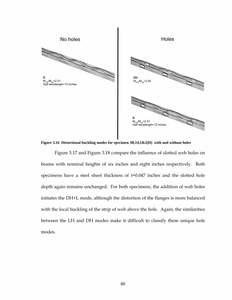
80

DMcrd/Myg=2.31Half wavelength=12 inches

DHMcrd/Myg=2.00

DMcrd/Myg=2.31Half wavelength=12 inches

No holes Holes

Figure 3.16 Distortional buckling modes for specimen 3B,14,1&2(H) with and without holes

Figure 3.17 and Figure 3.18 compare the influence of slotted web holes on

beams with nominal heights of six inches and eight inches respectively. Both

specimens have a steel sheet thickness of t=0.047 inches and the slotted hole

depth again remains unchanged. For both specimens, the addition of web holes

initiates the DH+L mode, although the distortion of the flanges is more balanced

with the local buckling of the strip of web above the hole. Again, the similarities

between the LH and DH modes make it difficult to classify these unique hole

modes.

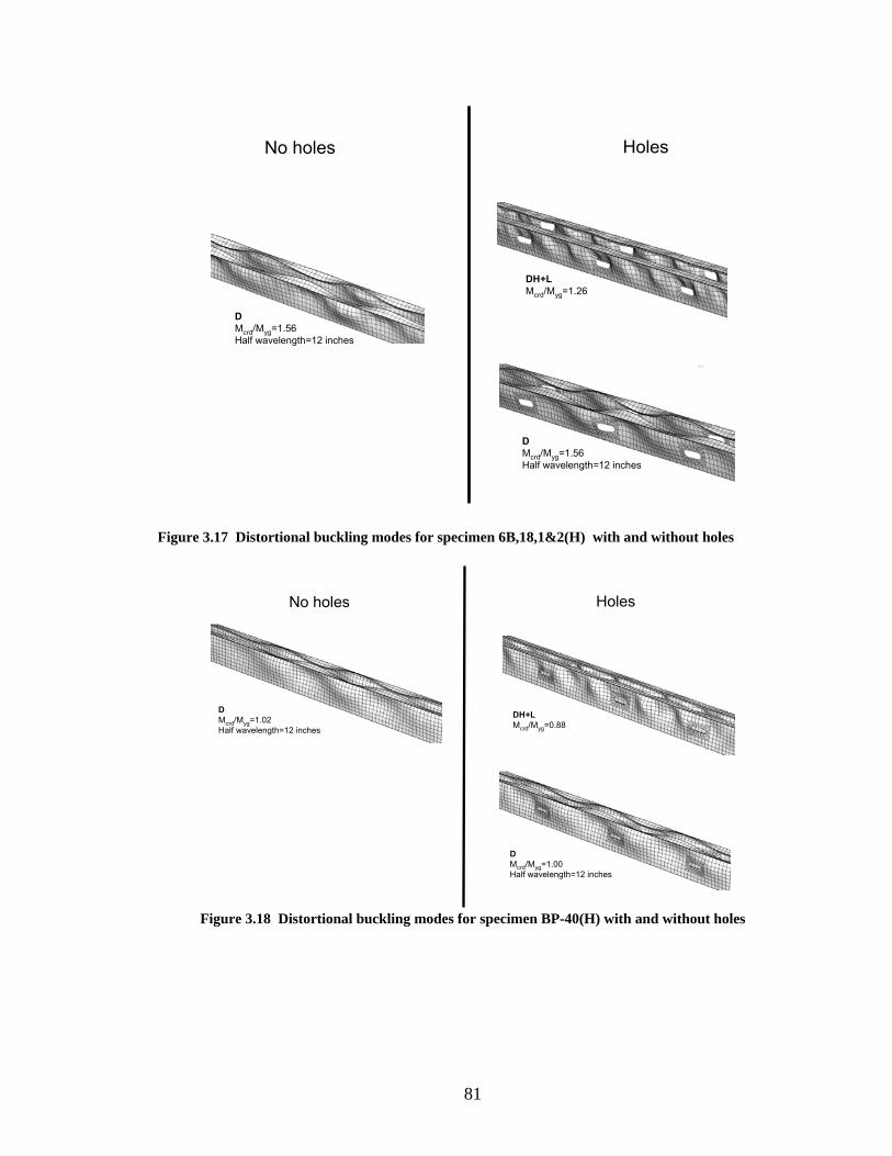
81

DMcrd/Myg=1.56Half wavelength=12 inches

DH+LMcrd/Myg=1.26

DMcrd/Myg=1.56Half wavelength=12 inches

No holes Holes

Figure 3.17 Distortional buckling modes for specimen 6B,18,1&2(H) with and without holes

DMcrd/Myg=1.02Half wavelength=12 inches

DH+LMcrd/Myg=0.88

DMcrd/Myg=1.00Half wavelength=12 inches

No holes Holes

Figure 3.18 Distortional buckling modes for specimen BP-40(H) with and without holes

82

D+LMcrd/Myg=1.03Half wavelength=11 inches

DMcrd/Myg=1.02Half wavelength=12 inches

No holes Holes

Figure 3.19 Distortional buckling modes for specimen 12B,16,1&2(H) with and without holes

The distortional buckling modes of the deepest beam specimen considered

in this study (nominal depth of 12 inches) are provided in Figure 3.19.

Identifying the distortional buckling modes for the channels making up this

beam are inherently challenging because even for a member without holes, there

is not a clear distinction between the L and D modes. The critical elastic buckling

moments for the beam channel cross section are provided at various half-

wavelengths from a finite strip analysis (CUFSM) in Figure 3.20. Only one

minimum exists, suggesting that the modes at or near the minimum buckling

load are a mixture of L and D modes. The most suitable mode identified by the

author (for the specimen without a hole) in Figure 3.19(a) actually alternates

between larger distortional half-waves and shorter local buckling half-waves in

the constant moment region of the channels. For the specimen with the web

holes in Figure 2.19(b), the local half-waves are not present and the mode

resembles more of a “pure” D mode. It is also noted that the DH mode is not

observed for this specimen. Although the changes in mode shapes are

83

interesting here, the key observation is that the holes do not influence the critical

elastic moment associated with the D mode for the small hhole/H considered

here.

LThis plot summarizes the modal participation (L, D, G, O) as a function of half-wavelength

D

Figure 3.20 Elastic buckling curve for 12” deep specimen with modal participation summarized,

note that selected L and D are mixed local-distortional modes

The influence of the web holes on the critical elastic buckling moment,

Mcrd, is summarized in Figure 3.21. Mcrd is defined as the minimum of the

critical elastic distortional buckling moments:

),,,min( 2211 CCCCcrd DDHDDHM =

where C1 and C2 designate the two channels that make up the beam specimen.

Mcrd decreases for most specimens with web holes when hhole/H>0.15. For

beams with hhole/H<0.15 (12 inch nominal depths beams in this study), Mcrd is

only slightly affected.

84

0 0.2 0.4 0.6 0.8 10

0.2

0.4

0.6

0.8

1

0 0.2 0.4 0.6 0.8 10

0.5

1

1.5

hhole/H

Mcr

d,ho

le/M

crd,

no h

ole

Figure 3.21 Influence of holes on Mcrd

The influence of the experiment boundary conditions on the distortional

buckling behavior is evaluated by comparing the critical elastic buckling moment

Mcrd(without holes) from the ABAQUS eigenbuckling analyses to the buckling

moment of each channel individually determined with the finite strip software

CUFSM. As was discussed in Section 3.4.1 for local buckling, the comparison of

ABAQUS and CUFSM results isolates the influence of the aluminum angle

straps, lateral bracing and the load application method on the critical elastic

moment results. Figure 3.22 demonstrates that the experiment test conditions

provide a significant boost to Mcrd which is hypothesized to be related to the

restrained distortional buckling caused by the aluminum angle straps. This

hypothesis is supported by existing research on unrestrained elastic distortional

85

beam buckling (no top flange connections) which observed similar CUFSM and

ABAQUS results (Yu and Schafer 2006). The pure D distortional half-

wavelengths from ABAQUS (without holes) in Figure 3.23 shorten or lengthen

relative to the predicted half-wavelengths from a finite strip analysis. This

change in half-wavelength away from the natural half-wavelength of the

distortional mode increases the critical elastic buckling moment. The influence

of the web holes on distortional half-wavelength in Figure 3.24 is less than that of

the experimental boundary conditions, with a general trend suggesting that pure

D distortional half-wavelength increases with increasing hhole/H.

0 0.2 0.4 0.6 0.8 10

0.2

0.4

0.6

0.8

1

0 50 100 150 200 250 3000

0.2

0.4

0.6

0.8

1

1.2

1.4

1.6

H/t

Mcr

d,no

hol

e, A

BAQ

US/M

crd,

CU

FSM

Figure 3.22 Influence of test boundary conditions on Mcrd

86

0 0.2 0.4 0.6 0.8 10

0.2

0.4

0.6

0.8

1

0 50 100 150 200 250 3000

0.5

1

1.5

H/t

half-

wav

elen

gth AB

AQU

S/hal

f-wav

elen

gth C

UFS

M

Figure 3.23 Influence of test boundary conditions on the distortional half-wavelength

0 0.2 0.4 0.6 0.8 10

0.2

0.4

0.6

0.8

1

0 0.2 0.4 0.6 0.8 10

0.5

1

1.5

hhole/H

half-

wav

elen

gth ho

le/h

alf-w

avel

engt

h no h

ole

Figure 3.24 Influence of holes on the distortional half-wavelength

87

3.4.3 Global buckling

Lateral-torsional buckling is a common global (G) elastic buckling mode in

beams, although this mode is eliminated for the specimens considered by

connecting the two Cee channels toe-to-toe with aluminum angles and by

providing lateral bracing at the compression flange in the constant moment

region of the beams (see Figure 3.3). Twisting of an individual channel about its

longitudinal axis is still possible though, even with the top flange restrained.

Figure 3.25 depicts the potential twisting mode. CUFSM is used to

conservatively quantify the elastic buckling moment for this mode, and it is

determined that Mcre is more than ten times the yield moment My for the

specimens in this study. Since the global elastic buckling moment, Mcre , does not

influence the DSM prediction as long as Mcre > 2.78 My , the global twisting

mode is not considered in this study. Refer to Section 3.5 for a description of the

DSM design equations for flexural members.

Lateral bracing of top flange

Figure 3.25 Possible global buckling mode occurs about the compression flange lateral brace point

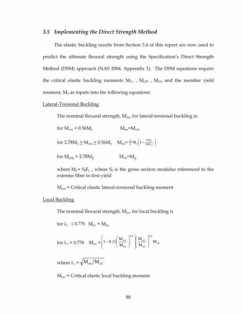
88

3.5 Implementing the Direct Strength Method

The elastic buckling results from Section 3.4 of this report are now used to

predict the ultimate flexural strength using the Specification’s Direct Strength

Method (DSM) approach (NAS 2004, Appendix 1). The DSM equations require

the critical elastic buckling moments Mcrl , Mcrd , Mcre and the member yield

moment, My as inputs into the following equations:

Lateral-Torsional Buckling

The nominal flexural strength, Mne, for lateral-torsional buckling is:

for Mcre < 0.56My Mne=Mcre

for 2.78My > Mcre > 0.56My Mne= ⎟⎠⎞⎜

⎝⎛ −

cre

y

M36M10

y910 1M

for Mcre > 2.78My Mne=My

where My= SfFy , where Sf is the gross section modulus referenced to the extreme fiber in first yield Mcre = Critical elastic lateral-torsional buckling moment

Local Buckling

The nominal flexural strength, Mnl, for local buckling is

for λl 776.0≤ Mnl = Mne

for λl > 0.776 Mnl = ne

4.0

ne

cr4.0

ne

cr MMM

MM

15.01 ⎟⎟⎠

⎞⎜⎜⎝

⎛

⎟⎟⎟

⎠

⎞

⎜⎜⎜

⎝

⎛

⎟⎟⎠

⎞⎜⎜⎝

⎛− ll

where λl = lcrne MM

Mcrl = Critical elastic local buckling moment

89

Distortional Buckling

The nominal flexural strength, Mnd, for distortional buckling is

for λd 673.0≤ Mnd = My

for λd > 0.673 Mnd = y

5.0

y

crd

5.0

y

crd MMM

MM22.01 ⎟

⎟⎠

⎞⎜⎜⎝

⎛

⎟⎟⎟

⎠

⎞

⎜⎜⎜

⎝

⎛

⎟⎟⎠

⎞⎜⎜⎝

⎛−

where λd = crdy MM

Mcrd = Critical elastic distortional buckling moment

The influence of the web holes on the Cee channel bending stiffness is negligible,

and therefore My is calculated with the gross strong axis moment of inertia. Mcrl

and Mcrd are assumed to be the minimum buckling moments of the beam:

),2,,,2,min( 222111 CCCCCCcr LLHLHLLHLHM =l

),,,min( 2211 CCCCcrd DDHDDHM =

where C1 and C2 denote the two Cee channels that make up the beam

specimens.

3.6 Comparison of DSM Predictions to Experiments

DSM moment predictions calculated with the procedure outlined in Section

3.5 are now compared to the ultimate beam moments for the 72 beam specimens

tested by Shan and LaBoube, Schuster, and Batson (Shan and LaBoube 1994).

The peak tested moment for each specimen, referred to as Mtest in this study, is

90

derived by multiplying Mut referenced in the Shan and LaBoube publication by

0.5 to obtain the peak moment per Cee channel.

DSM predicts that the ultimate strength of 36 of the 72 beams will be

controlled by local buckling. Figure 3.26 compares the tested capacities of these

beams to the DSM local buckling curve and reports the test-to-predicted ratio

statistics. The general trend of the tested data follows the DSM beam curve and

the mean test-to-predicted ratio is conservative.

Figure 3.27 compares the tested results to DSM predictions for the 28

distortional-buckling controlled specimens in this study. The curve is accurate

for members with higher slenderness but becomes slightly unconservative as

slenderness decreases. The mean-test-predicted ratio again suggests that the

DSM prediction is slightly unconservative for beam strengths controlled by

distortional buckling. A detailed investigation of this trend will be conducted in

the near future. The beams with higher slenderness ratios are typically the

deeper beams in this study (nominal depth of 12 inches), suggesting that these

beams are not influenced at ultimate limit state by the hole depth considered in

this study.

91

0 0.2 0.4 0.6 0.8 10

0.2

0.4

0.6

0.8

1

0 0.5 1 1.5 2 2.5 30

0.5

1

1.5

local slenderness, (Myg/Mcrl)0.5

Mte

st/M

yg

DSM Mnl

Local buckling controls

Test to Predictedmean=1.061STDV=0.096

Figure 3.26 Comparison of local-buckling controlled test data to DSM predictions

DSM predicts that eight beam specimens with relatively large sheet steel

thicknesses (t=0.077 inches) will fail by yielding of the Cee channel cross section.

The tested results are compared against the DSM column curves in Figure 3.28.

The data is distributed above and below the yield plateau of the column curve

with a mean test-to-predicted ratio of 0.96.

92

0 0.2 0.4 0.6 0.8 10

0.2

0.4

0.6

0.8

1

0 0.5 1 1.5 2 2.5 30

0.5

1

1.5

distortional slenderness, (Myg/Mcrd)0.5

Mte

st/M

yg

DSM Mnd

Distortional buckling controls

Test to Predictedmean=0.928STDV=0.098

Figure 3.27 Comparison of distortional buckling-controlled test data to DSM predictions

0 0.2 0.4 0.6 0.8 10

0.2

0.4

0.6

0.8

1

0 0.5 1 1.5 2 2.5 30

0.5

1

1.5

(Myg/Mcrl)0.5 or (Myg/Mcrd)0.5

Mte

st/M

yg

DSM Mnl

DSM Mnd

Yielding controls

Test to Predictedmean=0.960STDV=0.104

Figure 3.28 Comparison of yield-controlled test data to DSM predictions

93

Figure 3.29 summarizes all of the tested data and reports test-to-predicted

statistics for the entire study. Even with the variety of hhole/H considered in this

study, the data still follows the general trend of the beam curves. The mean test-

to-predicted ratio of 0.998 and standard deviation of 0.115 are also positive

indicators that the DSM approach can be used to accurately predict the strengths

of beams with holes.

0 0.2 0.4 0.6 0.8 10

0.2

0.4

0.6

0.8

1

0 0.5 1 1.5 2 2.5 30

0.5

1

1.5

(Myg/Mcrl)0.5 or (Myg/Mcrd)0.5

Mte

st/M

yg

DSM Mnl

DSM Mnd

Local buckling controlsDist. buckling controlsYielding controls

Test to Predictedmean=0.998STDV=0.115

Figure 3.29 Comparison of all test data to DSM predictions

94

3.7 Conclusions

The general research goal of this project is to expand the Direct Strength

Method to cold-formed steel members with holes. DSM was evaluated for

compression members with holes in Progress Report #1, and the lessons learned

are now applied in this study to evaluate DSM as strength predictor for beams

with holes. Eigenbuckling analyses of 72 beam specimens with slotted web holes

are performed and the resulting buckling modes identified and classified (Shan

and LaBoube 1994). The critical elastic buckling loads obtained from the

eigenbuckling analyses are then used in the current Specification’s DSM

formulation to predict the flexural strength of the beams with holes (NAS 2004,

Appendix 1). Conclusions from this study are summarized below.

Elastic Buckling

1. The slotted web holes create unique local and distortional elastic buckling

modes with critical loads less than the pure D and L modes.

2. The LH mode typically is the lowest critical elastic buckling load, and is

caused by the buckling of the strip of web above the hole in compression.

The LH mode resembles the assumed buckling mode in the “unstiffened

strip” approach in the Specification.

3. As was the case for compression members with holes, the DH mode is

again present in the compression flange of beams with holes. The DH

95

mode in beams has characteristics of the beam LH mode and is often

difficult to classify.

4. The critical elastic buckling moment associated with the pure L mode is

not influenced by typical experimental boundary conditions, but was

reduced by the slotted holes. The reduction varied with hhole/H with

similar trends to simply supported uniaxially compressed plates with

holes.

5. The critical elastic buckling moment associated with the pure D mode was

increased by the aluminum angle straps connecting the compression

flanges. The straps provided additional rotational stiffness which

changed the length of the distortional half-waves.

6. The metal sheet thickness influences the formation of mixed local-

distortional modes for the beams with slotted web holes. For thicker sheet

steel thicknesses pure DH and D modes formed, while for smaller

thicknesses DH+L and D+L were common.

Comparison of DSM Predictions to Tests

1. DSM is viable predictor of the flexural strengths of beams with holes

considered in this study. Predictions for specimens controlled by

distortional buckling were slightly unconservative while locally-

controlled specimen predictions were conservative.

2. DSM tended to be more accurate for beam specimens with small hhole/H.

96

3. The boost in the critical elastic buckling moment for the pure D mode

from the aluminum angles did not have a strong influence on the DSM

strength predictions because lower DH modes typically controlled.

3.8 Future Work

It can be concluded from the test-to-predicted results for both compression

members (Progress Report #1) and beams with holes (this report) that DSM is a

viable predictor of ultimate strength. The primary difficulty with using DSM to

predict the strength of members with holes is the effort required to accurately

obtain the elastic buckling modes. Developing finite element models with holes

is not for the faint-of-heart, and identifying elastic buckling modes manually is

time-consuming and at some level subjective.

Future work will continue with elastic buckling studies that evaluate

parameters such as hole shape, size, spacing, and location. A heavy emphasis

will also be placed on simplifying the procedures for obtaining critical elastic

buckling loads, for example:

• developing a hand calculation to approximate the critical elastic buckling

moment for the DH and LH modes.

• implementing recently developed modal decomposition methods to

automatically identify and classify elastic buckling modes.

• creating more user friendly FE meshing tools and software

97

The failure modes of beams with holes are also important when attempting to

connect elastic buckling modes to ultimate flexural strength. Nonlinear finite

element analysis will be used to consider the influence of imperfections and

residual stresses on flexural ultimate strength, and parameter studies will be

conducted to connect specific failure modes of beams with holes to elastic

buckling shapes and strength.

4 Future Work

The research summarized in this report and in Progress Reports #1 and #2

represents a substantial portion of the investigatory work planned for this

project. This knowledge base will now allow us to define more focused research

goals as we strive to validate a Direct Strength Method approach for members

with holes.

What we have learned so far…

The presence of holes creates unique local and distortional elastic buckling

modes in both beams (LH, LH2, DH) and columns (DH and DH2). The critical

elastic buckling loads associated with these modes can be used successfully

within the Specification’s DSM approach to make strength predictions for Cee

channel beams and columns that are generally consistent with tested results.

Nonlinear finite element modeling of rectangular plates and stub columns with

slotted web holes demonstrated that material yielding may occur first in the

vicinity of the hole, which then influences the distribution of load and the

98

deformation of the member at and beyond the peak load. This “net section”

influence does not always come into play though, as in the case of compression

members where the width of the hole is small relative to the width of the web. In

the column experiments described in this report, we observe firsthand the

connection between buckling and load-deformation response. The slotted web

holes modify the local and distortional buckling half-waves in the short and

intermediate length columns, either decreasing or increasing the stiffness and

ductility of the columns.

Where we are headed…

We are encouraged that our as research has revealed common trends and

ideas relating elastic buckling and ultimate strength for cold-formed steel

members with holes. Future research will continue by validating the DSM

approach for industry-standard beam and column cross sections with holes and

by improving the tools used to predict and identifying elastic buckling modes for

members with holes. The column experiments described in this report will be

used to verify our nonlinear finite element modeling methodology, including the

methods we use to model initial imperfections and residual stresses. Once our

models are verified, we plan to determine the ultimate strengths for a range of

industry standard beam and column products with nonlinear FEM and compare

them to DSM predictions. Close attention will also be paid to the influence of

initial imperfections (in the shape of local and distortional elastic buckling

99

modes) on the load-deformation response and failure progression for these

members with holes.

Once an eigenbuckling analysis is complete, the identification of the

elastic buckling modes is performed by evaluating each mode one by one.

Future research will determine the feasibility of using simplified hand-methods

that predict the critical elastic buckling modes of local hole modes (LH, DH) in

combination with finite strip buckling predictions to circumvent the modeling of

the full member. Also, the recently developed modal decomposition methods for

cold-formed steel members (Ádàny and Schafer 2006) will be evaluated as a tool

for automating the modal identification process.

100

References ABAQUS (2004). ABAQUS/Standard Users Manual version 6.5. ABAQUS, Inc., www.abaqus.com, Providence, RI. Ádàny, S., Schafer, B.W., (2006) “Buckling mode decomposition of single-branched open cross-section members via the finite strip method.” Thin-Walled Structures, 44, 585-600. ASTM. (2004). “E 8M-04, Standard Test Methods for Tension Testing of Metallic Materials (Metric).” ASTM International, West Conshohocken, PA. LabVIEW. (2005). LabVIEW version 8. National Instruments, www.labview.com, Austin, TX. Batson, K.D. (1992). “Flexural Behavior of Webs with Openings.” M.S. Thesis, University of Missouri-Rolla. Galambos, T. (1998). “ Appendix B.3, Technical Memorandum No.3: Stub-Column Test Procedure.” Guide to Stability Design Criteria for Metal Structures. 5th ed., Wiley, New York, NY, 815-822. Miller, T.H., Peköz, T. (1989). “Studies on the behavior of cold-formed steel wall stud assemblies.” Final Report, Cornell University, Ithaca, NY. Miller, T.H., Peköz, T. (1994). “Unstiffened strip approach for perforated wall studs.” Journal of Structural Engineering, ASCE, Vol. 120, No. 2. Ziemian, R., McGuire, W. (2005). MASTAN version 3.0.4. Bucknell University, Lewisburg, PA. Moen, C., Schafer, B.W. (2006). “Direct strength design for cold-formed steel members with perforations.” Progress Report #1, American Iron and Steel Institute, Washington, D.C. Moen, C, Schafer B.W. (2006). “Impact of holes on the elastic buckling of cold-formed steel columns with applications to the Direct Strength Method.” 18th Int’l Spec. Conf. on Cold-Formed Steel Structures, Orlando, FL. North American Specification (NAS). (2001). “AISI TS-2-02, Stub Column Test Method for Effective Area of Cold-Formed Steel Columns.” 2001 North American Cold Formed Steel Specification, American Iron and Steel Institute, Washington, D.C.

101

North American Specification (NAS). (2004). 2004 Supplement to the North American Specification for the Design of Cold-Formed Steel Structures. American Iron and Steel Institute, Washington, D.C. Schafer, B.W., Ádàny, S. (2006) “Buckling analysis of cold-formed steel members using CUFSM: conventional and constrained finite strip methods.” Proceedings, 18th International Specialty Conference on Cold-Formed Steel Structures, Orlando, FL (2006). Schuster, R.M. (1992). “Testing of Perforated C-Stud Sections in Bending.” University of Waterloo, Ontario, Canada. Shan, M.Y., LaBoube, R.A. (1994). “Behavior of Web Elements With Openings Subjected to Bending, Shear, and the Combination of Bending and Shear.” Civil Engineering Study 94-2, Cold-Formed Steel Series, University of Missour-Rolla. Yu, C., Schafer, B.W. (2006). “Effect of longitudinal stress gradient on the ultimate strength of thin plates.” Thin-Walled Structures, 44(7), 787-799. Yu, C., Schafer, B.W. (2006). “Distortional buckling tests on cold-formed steel beams.” ASCE Journal of Structural Engineering, 132(4), 515-528.

102

Appendix A – Column Experiment Results

103

Column Specimen 362-1-24-NH

0 0.05 0.1 0.15 0.2

-14

-12

-10

-8

-6

-4

-2

0

Column axial displacement (inches)

Col

umn

axia

l load

(kip

s)

Ptest=10.48 kips

362-1-24-NH

0 0.05 0.1 0.15 0.2-1.5

-1

-0.5

0

0.5

1

1.5

Column axial displacement (inches)

Flan

ge d

ispl

acem

ent (

inch

es)

362-1-24-NH

WE

Notes: Loaded N to S instead of S to N. Adjusted all geometry measurements. Lips rotated and not touching bottom platen after peak load.

104

Column Specimen 362-2-24-NH

Peak Load

0 0.05 0.1 0.15 0.2

-14

-12

-10

-8

-6

-4

-2

0

Column axial displacement (inches)

Col

umn

axia

l load

(kip

s)

Ptest=10.51 kips

362-2-24-NH

0 0.05 0.1 0.15 0.2-1.5

-1

-0.5

0

0.5

1

1.5

Column axial displacement (inches)

Flan

ge d

ispl

acem

ent (

inch

es)

362-2-24-NH

WE

Notes:

105

Column Specimen 362-3-24-NH

Peak Load

0 0.05 0.1 0.15 0.2

-14

-12

-10

-8

-6

-4

-2

0

Column axial displacement (inches)

Col

umn

axia

l load

(kip

s)

Ptest=10.15 kips

362-3-24-NH

0 0.05 0.1 0.15 0.2-1.5

-1

-0.5

0

0.5

1

1.5

Column axial displacement (inches)

Flan

ge d

ispl

acem

ent (

inch

es)

362-3-24-NH

WE

Notes: Bottom lips rotated at 7 kips post-peak and are not bearing on platen.

106

Column Specimen 362-1-24-H

Peak Load

0 0.05 0.1 0.15 0.2

-14

-12

-10

-8

-6

-4

-2

0

Column axial displacement (inches)

Col

umn

axia

l load

(kip

s)

Ptest=10.01 kips

362-1-24-H

0 0.05 0.1 0.15 0.2-1.5

-1

-0.5

0

0.5

1

1.5

Column axial displacement (inches)

Flan

ge d

ispl

acem

ent (

inch

es)

362-1-24-H

WE

Notes: Visible buckling of web on either side of hole at 7 kips.

107

Column Specimen 362-2-24-H

0 0.05 0.1 0.15 0.2

-14

-12

-10

-8

-6

-4

-2

0

Column axial displacement (inches)

Col

umn

axia

l load

(kip

s)

Ptest=10.38 kips

362-2-24-H

0 0.05 0.1 0.15 0.2-1.5

-1

-0.5

0

0.5

1

1.5

Column axial displacement (inches)

Flan

ge d

ispl

acem

ent (

inch

es)

362-2-24-H

WE

Notes: Visible buckling of web on either side of hole at 5 kips.

Peak Load

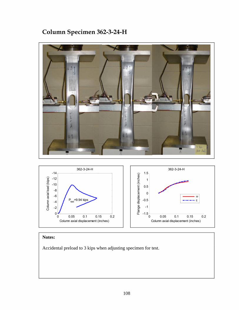
108

Column Specimen 362-3-24-H

0 0.05 0.1 0.15 0.2

-14

-12

-10

-8

-6

-4

-2

0

Column axial displacement (inches)

Col

umn

axia

l load

(kip

s)

Ptest=9.94 kips

362-3-24-H

0 0.05 0.1 0.15 0.2-1.5

-1

-0.5

0

0.5

1

1.5

Column axial displacement (inches)

Flan

ge d

ispl

acem

ent (

inch

es)

362-3-24-H

WE

Notes: Accidental preload to 3 kips when adjusting specimen for test.

109

Column Specimen 362-1-48-NH

Peak Load

0 0.05 0.1 0.15 0.2

-14

-12

-10

-8

-6

-4

-2

0

Column axial displacement (inches)

Col

umn

axia

l load

(kip

s)

Ptest=9.09 kips

362-1-48-NH

0 0.05 0.1 0.15 0.2-1.5

-1

-0.5

0

0.5

1

1.5

Column axial displacement (inches)

Flan

ge d

ispl

acem

ent (

inch

es)

362-1-48-NH

WE

Notes: Good end conditions – no visible gaps. 9 kips – a metallic noise – yielding of west flange and increase in local wavelengths. Column failed by global-torsional collapse.

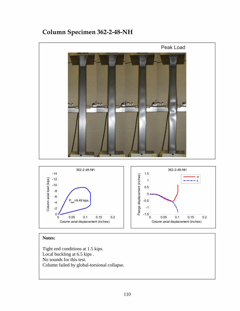
110

Column Specimen 362-2-48-NH

Peak Load

0 0.05 0.1 0.15 0.2

-14

-12

-10

-8

-6

-4

-2

0

Column axial displacement (inches)

Col

umn

axia

l load

(kip

s)

Ptest=9.49 kips

362-2-48-NH

0 0.05 0.1 0.15 0.2-1.5

-1

-0.5

0

0.5

1

1.5

Column axial displacement (inches)

Flan

ge d

ispl

acem

ent (

inch

es)

362-2-48-NH

WE

Notes: Tight end conditions at 1.5 kips. Local buckling at 6.5 kips . No sounds for this test. Column failed by global-torsional collapse.

111

Column Specimen 362-3-48-NH

Peak Load

0 0.05 0.1 0.15 0.2

-14

-12

-10

-8

-6

-4

-2

0

Column axial displacement (inches)

Col

umn

axia

l load

(kip

s)

Ptest=9.48 kips

362-3-48-NH

0 0.05 0.1 0.15 0.2-1.5

-1

-0.5

0

0.5

1

1.5

Column axial displacement (inches)

Flan

ge d

ispl

acem

ent (

inch

es)

362-3-48-NH

WE

Notes: Local buckling first observed at 6.5 kips. Local wavelengths lengthen at 8.5 kips. Yielding of flange lips at 9 kips (near peak). Column failed by global-torsional collapse.

112

Column Specimen 362-1-48-H

Peak Load

0 0.05 0.1 0.15 0.2

-14

-12

-10

-8

-6

-4

-2

0

Column axial displacement (inches)

Col

umn

axia

l load

(kip

s)

Ptest=8.95 kips

362-1-48-H

0 0.05 0.1 0.15 0.2-1.5

-1

-0.5

0

0.5

1

1.5

Column axial displacement (inches)

Flan

ge d

ispl

acem

ent (

inch

es)

362-1-48-H

WE

Notes: No visible gaps and ends under 1 kip. Local buckling is visible at 7 kips. Local half-waves merge at 8.5 kips. Bulging of web at hole occurs near peak load. Column failed by global-torsional collapse.

113

Column Specimen 362-2-48-H

Peak Load

0 0.05 0.1 0.15 0.2

-14

-12

-10

-8

-6

-4

-2

0

Column axial displacement (inches)

Col

umn

axia

l load

(kip

s)

Ptest=9.18 kips

362-2-48-H

0 0.05 0.1 0.15 0.2-1.5

-1

-0.5

0

0.5

1

1.5

Column axial displacement (inches)

Flan

ge d

ispl

acem

ent (

inch

es)

362-2-48-H

WE

Notes: End conditions tight at 4 kips. Local buckling visible at 6.5 kips. Distortional buckling seems to increase as load-displacement softens. East LVDT reaches limit of range as column starts to twist. Column failed by global-torsional collapse.

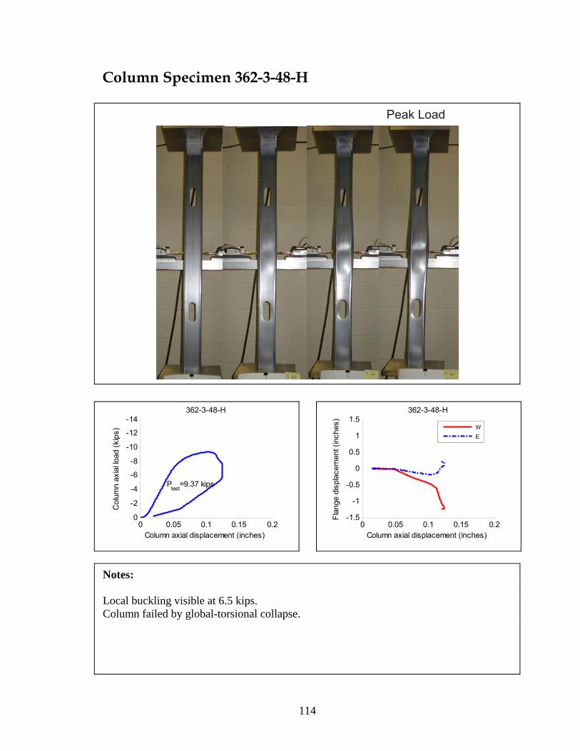
114

Column Specimen 362-3-48-H

Peak Load

0 0.05 0.1 0.15 0.2

-14

-12

-10

-8

-6

-4

-2

0

Column axial displacement (inches)

Col

umn

axia

l load

(kip

s)

Ptest=9.37 kips

362-3-48-H

0 0.05 0.1 0.15 0.2-1.5

-1

-0.5

0

0.5

1

1.5

Column axial displacement (inches)

Flan

ge d

ispl

acem

ent (

inch

es)

362-3-48-H

WE

Notes: Local buckling visible at 6.5 kips. Column failed by global-torsional collapse.

115

Column Specimen 600-1-24-NH

Peak Load

0 0.05 0.1 0.15 0.2

-14

-12

-10

-8

-6

-4

-2

0

Column axial displacement (inches)

Col

umn

axia

l load

(kip

s)

Ptest=11.93 kips

600-1-24-NH

0 0.05 0.1 0.15 0.2-1.5

-1

-0.5

0

0.5

1

1.5

Column axial displacement (inches)

Flan

ge d

ispl

acem

ent (

inch

es)

600-1-24-NH

WE

Notes: Local and distortional waves seem to stay separate. 8 kips (post-peak) – east flange buckles.

116

Column Specimen 600-2-24-NH

Peak Load

0 0.05 0.1 0.15 0.2

-14

-12

-10

-8

-6

-4

-2

0

Column axial displacement (inches)

Col

umn

axia

l load

(kip

s)

Ptest=11.95 kips

600-2-24-NH

0 0.05 0.1 0.15 0.2-1.5

-1

-0.5

0

0.5

1

1.5

Column axial displacement (inches)

Flan

ge d

ispl

acem

ent (

inch

es)

600-2-24-NH

WE

Notes: Web has large curve when placing specimen on bottom platen. Visible gap between platen and specimen at top west web-flange corner - 5 kips. 10 kips (post-peak)- flanges buckle and lose contact with bottom platen.

117

Column Specimen 600-3-24-NH

Peak Load

0 0.05 0.1 0.15 0.2

-14

-12

-10

-8

-6

-4

-2

0

Column axial displacement (inches)

Col

umn

axia

l load

(kip

s)

Ptest=12.24 kips

600-3-24-NH

0 0.05 0.1 0.15 0.2-1.5

-1

-0.5

0

0.5

1

1.5

Column axial displacement (inches)

Flan

ge d

ispl

acem

ent (

inch

es)

600-3-24-NH

WE

Notes: Specimen failed at bottom end condition, web rolled over and was not bearing on platen.

118

Column Specimen 600-1-24-H

Peak Load

0 0.05 0.1 0.15 0.2

-14

-12

-10

-8

-6

-4

-2

0

Column axial displacement (inches)

Col

umn

axia

l load

(kip

s)

Ptest=12.14 kips

600-1-24-H

0 0.05 0.1 0.15 0.2-1.5

-1

-0.5

0

0.5

1

1.5

Column axial displacement (inches)

Flan

ge d

ispl

acem

ent (

inch

es)

600-1-24-H

WE

Notes: Slight gap at east top web-flange corner - 3 kips, gap is closed at 11 kips. East flange gives way at 11 kips with dip in load-disp. curve, may be related to above. Loud popping sound at 8 kips (post-peak) and large change in load-displ. slope.

119

Column Specimen 600-2-24-H

Peak Load

0 0.05 0.1 0.15 0.2

-14

-12

-10

-8

-6

-4

-2

0

Column axial displacement (inches)

Col

umn

axia

l load

(kip

s)

Ptest=11.62 kips

600-2-24-H

0 0.05 0.1 0.15 0.2-1.5

-1

-0.5

0

0.5

1

1.5

Column axial displacement (inches)

Flan

ge d

ispl

acem

ent (

inch

es)

600-2-24-H

WE

Notes: Specimen failure mode similar to that of a no-hole specimen.

120

Column Specimen 600-3-24-H

Peak Load

0 0.05 0.1 0.15 0.2

-14

-12

-10

-8

-6

-4

-2

0

Column axial displacement (inches)

Col

umn

axia

l load

(kip

s)

Ptest=11.79 kips

600-3-24-H

0 0.05 0.1 0.15 0.2-1.5

-1

-0.5

0

0.5

1

1.5

Column axial displacement (inches)

Flan

ge d

ispl

acem

ent (

inch

es)

600-3-24-H

WE

Notes: Good contact with platens.

121

Column Specimen 600-1-48-NH

Peak Load

0 0.05 0.1 0.15 0.2

-14

-12

-10

-8

-6

-4

-2

0

Column axial displacement (inches)

Col

umn

axia

l load

(kip

s)

Ptest=11.15 kips

600-1-48-NH

0 0.05 0.1 0.15 0.2-1.5

-1

-0.5

0

0.5

1

1.5

Column axial displacement (inches)

Flan

ge d

ispl

acem

ent (

inch

es)

600-1-48-NH

WE

Notes: Local buckling first observed at 4.5 kips (11 half-waves). Distortional wave becomes prominent at 10 kips. Loud noises 1 minute apart – L waves turn to D waves at north, then south ends.

122

Column Specimen 600-2-48-NH

Peak Load

0 0.05 0.1 0.15 0.2

-14

-12

-10

-8

-6

-4

-2

0

Column axial displacement (inches)

Col

umn

axia

l load

(kip

s)

Ptest=11.44 kips

600-2-48-NH

0 0.05 0.1 0.15 0.2-1.5

-1

-0.5

0

0.5

1

1.5

Column axial displacement (inches)

Flan

ge d

ispl

acem

ent (

inch

es)

600-2-48-NH

WE

Notes: Gap between platen and specimen at top east flange-web corner closes at 2 kips. Can see distortional shape developing at 4.5 kips. Local buckling visible at 5 kips. Two loud bangs (peak load, 10.5 kips post peak) – local web waves change to D waves. Flange distortion slows at 7 kips post-peak.

123

Column Specimen 600-3-48-NH

Peak Load

0 0.05 0.1 0.15 0.2

-14

-12

-10

-8

-6

-4

-2

0

Column axial displacement (inches)

Col

umn

axia

l load

(kip

s)

Ptest=11.29 kips

600-3-48-NH

0 0.05 0.1 0.15 0.2-1.5

-1

-0.5

0

0.5

1

1.5

Column axial displacement (inches)

Flan

ge d

ispl

acem

ent (

inch

es)

600-3-48-NH

WE

Notes: Gap between platen and specimen at east top flange closes at 1 kip. Loud sound at peak load – L waves change to D waves in web.

124

Column Specimen 600-1-48-H

Peak Load

0 0.05 0.1 0.15 0.2

-14

-12

-10

-8

-6

-4

-2

0

Column axial displacement (inches)

Col

umn

axia

l load

(kip

s)

Ptest=11.16 kips

600-1-48-H

0 0.05 0.1 0.15 0.2-1.5

-1

-0.5

0

0.5

1

1.5

Column axial displacement (inches)

Flan

ge d

ispl

acem

ent (

inch

es)

600-1-48-H

WE

Notes: Local buckling and DH mode visible at 5 kips. Loud noise at 9.5 kips – L waves changes to D wave in web.

125

Column Specimen 600-2-48-H

Peak Load

0 0.05 0.1 0.15 0.2

-14

-12

-10

-8

-6

-4

-2

0

Column axial displacement (inches)

Col

umn

axia

l load

(kip

s)

Ptest=11.7 kips

600-2-48-H

0 0.05 0.1 0.15 0.2-1.5

-1

-0.5

0

0.5

1

1.5

Column axial displacement (inches)

Flan

ge d

ispl

acem

ent (

inch

es)

600-2-48-H

WE

Notes: Local buckling visible at 4 kips. D wave interrupted by large crease. L web waves change to D waves (9 kips post-peak, 7.5 kips post-peak)

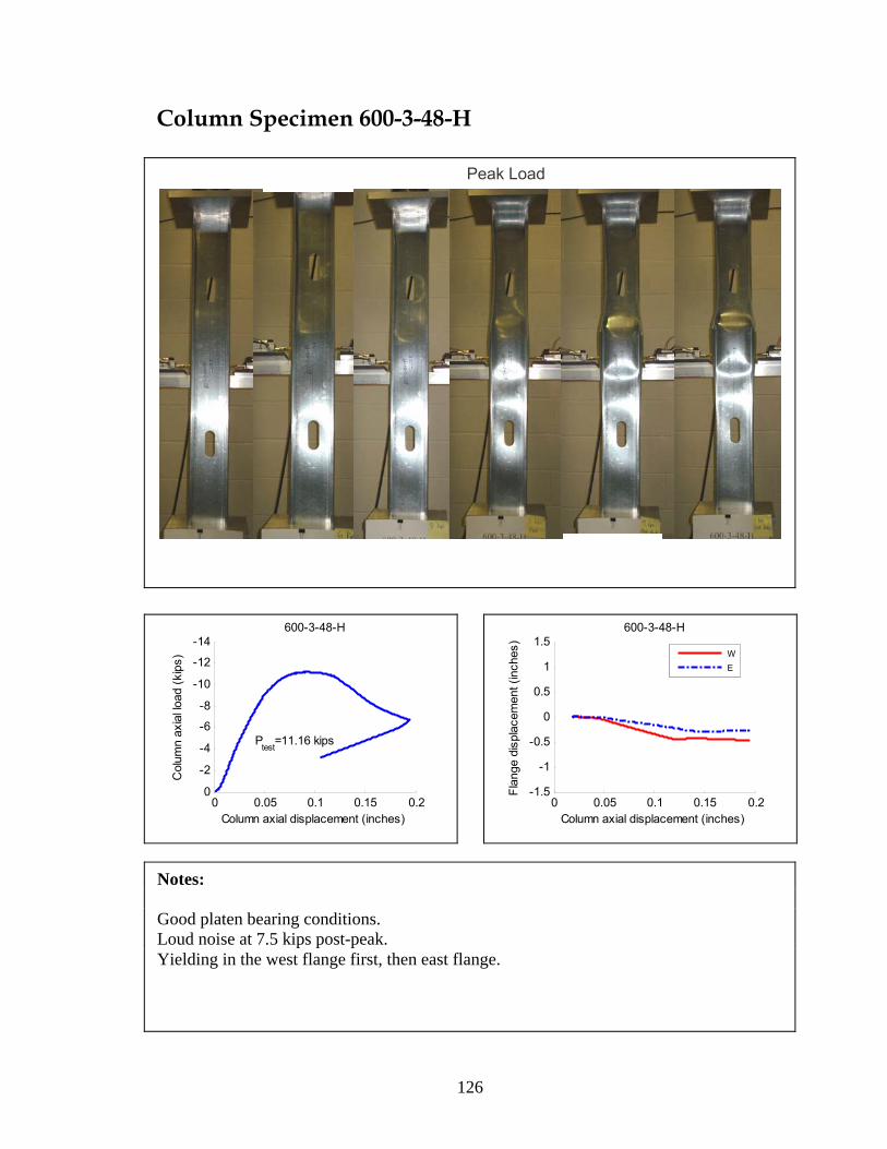
126

Column Specimen 600-3-48-H

Peak Load

0 0.05 0.1 0.15 0.2

-14

-12

-10

-8

-6

-4

-2

0

Column axial displacement (inches)

Col

umn

axia

l load

(kip

s)

Ptest=11.16 kips

600-3-48-H

0 0.05 0.1 0.15 0.2-1.5

-1

-0.5

0

0.5

1

1.5

Column axial displacement (inches)

Flan

ge d

ispl

acem

ent (

inch

es)

600-3-48-H

WE

Notes: Good platen bearing conditions. Loud noise at 7.5 kips post-peak. Yielding in the west flange first, then east flange.

127