Direct Strength Design for Cold-Formed Steel Members with Perforations Holes Progress... ·...

Direct Strength Design for Cold-Formed Steel Members

with Perforations

Progress Report 4C. Moen and B.W. Schafer

AISI-COS MeetingJuly 2007

Outline• Objective• Summary of past progress• FEA of Columns with holes

– Modeling approach– Elastic buckling– Nonlinear modeling to collapse– Comparison with testing from progress report 3

• Developing DSM for columns with holes– Impact of gross vs. net area decisions on strength– Comparison of predictions for available column tests

• Conclusions• Future Work

to becovered intask groupmeeting

ObjectiveDevelopment of a general design method

for cold-formed steel members with perforations.

Direct Strength Method ExtensionsPn = f (Py, Pcre, Pcrd, Pcrl)?

How do the DSMcurves need tochange?

Gross or net, or some combination?

Explicitly model hole(s)?Accuracy? Efficiency?Identification? Just thesemodes?

Progress Report 1 & 2 HighlightElastic Buckling Modes in a Column

Pcrd=1.15Py,g

Pcrl=0.42Py,g Pcrl=0.42Py,g

Pcrd1=0.52Py,g

Pcrd2=0.54Py,g

Pcrd3=1.16Py,g

D

L L

L+DH

DH2

D+L

Distortional modes unique to a column with a hole

Unique D modes are created with the presence of a hole

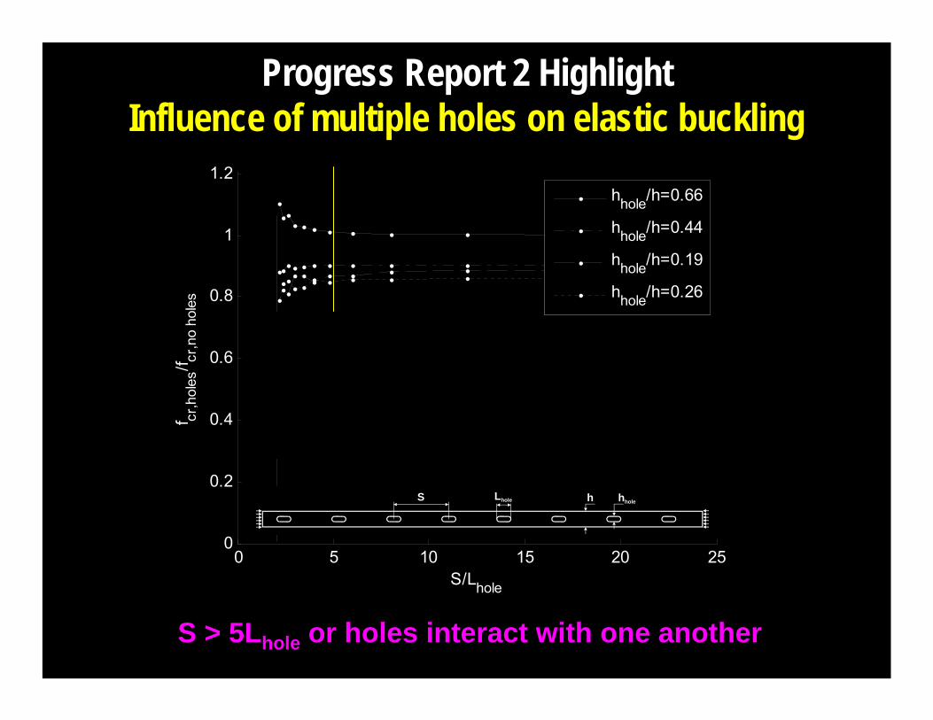
Progress Report 2 HighlightInfluence of multiple holes on elastic buckling

0 0.2 0.4 0.6 0.8 10

0.2

0.4

0.6

0.8

1

0 5 10 15 20 250

0.2

0.4

0.6

0.8

1

1.2

S/Lhole

f cr,h

oles

/f cr,n

o ho

les

hhole/h=0.66

hhole/h=0.44

hhole/h=0.19

hhole/h=0.26

2 3 4 50.75

0.8

0.85

0.9

S/Lhole

0

S Lhole hholeh

Decrease in fcr when hole spacing becomes small

S > 5Lhole or holes interact with one another

Progress Report 2 HighlightCritical buckling stress equation

0 0.2 0.4 0.6 0.8 10

0.2

0.4

0.6

0.8

1

0 0.2 0.4 0.6 0.8 10

0.5

1

1.5

2

2.5

3

3.5

4

4.5

5

hhole/h

plat

e bu

cklin

g co

eff.,

k

Data points from eigenbuckling analysis

Fitted curve

44462

≤+⎟⎠⎞

⎜⎝⎛−⎟

⎠⎞

⎜⎝⎛=

hh

hhk holehole

SS/2 Lhole hholeh

for S/Lhole > 5

If holes do not interact simplified elastic local buckling predictions are certainly possible.

Progress Report 3 HighlightBeams: finding Mcrl, Mcrd, Mcre for tests

Beam end restrained in 2 and 3 (v, w=0)

Beam end restrained in 2 and 3 (v, w=0)

Bottom flange restrained in 1 at support (u=0)

* **

**

**

**

Restrain node at midline of top flange in 3 (w=0) (Typ.)

Rigid body connection between top (and bottom) flange midline nodes (Typ.)

1

2

3

Care is taken to simulate tested boundary conditions in eigenbuckling analyses.

Progress Report 3 HighlightImpact of Hole on Beam Local Buckling

0 0.2 0.4 0.6 0.8 10

0.2

0.4

0.6

0.8

1

0 0.2 0.4 0.6 0.8 10

0.5

1

1.5

hhole/H

Mcrl ,h

ole/M

crl ,n

o ho

le

Largest decrease in critical elastic local buckling moment occurs at hhole/h= 0.25

Progress Report 3 HighlightImpact of Hole on Beam Distortional Buckling

0 0.2 0.4 0.6 0.8 10

0.2

0.4

0.6

0.8

1

0 0.2 0.4 0.6 0.8 10

0.5

1

1.5

hhole/H

Mcr

d,ho

le/M

crd,

no h

ole

Holes decrease critical elastic distortional buckling moment, modeling required

Progress Report 3 HighlightColumn tests

Progress Report 3 HighlightStrength Results from Column Tests

Holes have a small influence on compressive strength here BUT…

Ptest Mean Std. Dev.kips kips kips

362-1-24-NH 10.48362-2-24-NH 10.51362-3-24-NH 10.15362-1-24-H 10.00362-2-24-H 10.38362-3-24-H 9.94362-1-48-NH 9.09362-2-48-NH 9.49362-3-48-NH 9.48362-1-48-H 8.95362-2-48-H 9.18362-3-48-H 9.37600-1-24-NH 11.93600-2-24-NH 11.95600-3-24-NH 12.24600-1-24-H 12.14600-2-24-H 11.62600-3-24-H 11.79600-1-48-NH 11.15600-2-48-NH 11.44600-3-48-NH 11.29600-1-48-H 11.16600-2-48-H 11.70600-3-48-H 11.16

11.29

Specimen

10.38

10.11

9.35

11.34

0.20

0.24

0.23

0.21

0.17

0.27

0.15

0.31

9.17

Hole

Without Hole Short

ColumnsHole

12.04

11.85

Without Hole Long

ColumnsHole

362S162-33

600S162-33

Without Hole Long

ColumnsHole

Without Hole Short

Columns

Progress Report 3 Highlight362S162-33 Short Column

0 0.2 0.4 0.6 0.8 10

0.2

0.4

0.6

0.8

1

0 0.05 0.1 0.15 0.2

-14

-12

-10

-8

-6

-4

-2

0

Column axial displacement (inches)

Col

umn

axia

l loa

d (k

ips)

362-2-24-NH362-2-24-H

Slotted hole influences post-peak load path and decreases column ductility.

FEA modeling• Objective: Develop a reliable FEA modeling

procedure/guidelines for CFS sections with holes modeled to collapse loads.

• Motivation: Available test database is limited, e.g., insufficient data on intermediate length columns with holes in local and distortional buckling, long columns with holes, holes in the flanges, etc.

• Method: Develop/improve modeling guidelines based on comparisons with testing conducted at JHU then expand to needed parametric studies

Jump to next section

FEA Modeling of Column Tests

• Begin with elastic buckling– necessary for DSM-style predictions– mode shapes are typically used as

imperfections in nonlinear models• Then move on to collapse modeling

(full nonlinear FEA models)

Elastic buckling (24 in. columns)

24” long 362 specimens

Local Buckling (L) Distortional Buckling

Hole terminates web local buckling asymmetric

distortional hole mode with local buckling at the hole

Hole shifted off centerline web

DDH+LD

Local Buckling Distortional Buckling

Holes change number of half-waves from 8 (NH) to 12 (H)

Holes cause mixed distortional – local mode

D DH+L

Elastic buckling (48 in. columns)

48” long 600 specimens

Mean STDEV Mean STDEV600s 1.01 0.03 1.19 0.18362s 1.01 0.01 1.09 0.10no holes 0.99 0.00 1.16 0.09holes 1.00 0.02 1.12 0.1948" specimens 1.01 0.02 1.03 0.0524" specimens 1.01 0.03 1.17 0.15

Distortional BucklingABAQUS/CUFSM

Local BucklingSpecimen Group

Comparison of buckling to CUFSM

Holes do not influence local.. Pcrl

(b) 600s have longer distortional buckling half-wavelength thus are more influenced by fix-fix boundary

(c) holes have only a small impact –but large variance....

(d) Shorter specimens more influenced by fix-fix boundary

FIX-FIX B.C. / PIN-PIN B.C.

b

c

d

a

b

c

d

Typical* Nonlinear FEA modeling of CFS• General:

Shell element model in ABAQUS• Solution control:

Riks (arc-length method)• Boundary Conditions:

idealized, perfect pin, perfect fixity• Material modeling:

σ-ε from flats, von Mises criteria, isotropic hardening• Geometric Imperfections:

buckling mode shapes superposed on ideal geometry, magnitude from Schafer and Peköz (1998)

• Residual Stresses: ignored

• Cold work of forming: ignored

*typical of modeling conducted in Schafer’s group

Nonlinear FEA modeling of CFS to collapse• General:

Shell element model in ABAQUS• Solution control:

Riks (arc-length method) & Stabilize (artificial damping)• Boundary Conditions:

model contact, friction, liftoff from end platens• Material modeling:

σ-ε from flats, von Mises criteria, isotropic hardening• Geometric Imperfections:

buckling mode shapes superposed on averagegeometry, magnitude from simple measurements

• Residual Stresses: in the corners, with realistic through thickness variation

• Cold work of forming: in the corners through inclusion of plastic strain, varies through the thickness, not your usual cold work...

Boundary conditions modeling

Friction-bearing end conditions are modeled in ABAQUS

1

2

3

45

6

ABAQUS Analytical Rigid Surface (Typ.)

Restrain rigid surface reference node in 2 to 6 directions

Restrain rigid surface reference node in 1 to 6 directions

Apply imposed displacement of surface in 1 direction

Assign friction contact behavior in ABAQUS between rigid surface and specimen

ABAQUS contact modeling captures lift off of lip for 600 specimen

Boundary conditions local response

specimen/model600-2-24-NH

0 0.05 0.1 0.15 0.20

2

4

6

8

10

12

14

16

18

20

axial displacement, in.

colu

mn

axia

l loa

d, k

ips

Contact SurfaceFixed-Fixed

The failure response with friction-bearing boundary conditions is similar to that with fixed-fixed boundary conditions

Boundary conditions global response

specimen/model600-2-24-NH

0 0.05 0.1 0.15 0.20

2

4

6

8

10

12

14

16

18

20


colu

mn

axia

l loa

d, k

ips

Artificial DampingModified RiksExperiment

Artificial damping predicts stronger, more ductile response than the Riks Method

Cross section slips on platen in Riks Method here, no slip observed with artificial damping

Solution control sensitivity(and boundary conditions)

specimen/model600-2-24-NH artificial damping is more robust, but artificially high?

Eigenmodes & imperfection shapes

Hole is filled in with S9R5 elements to produce no hole local buckling shape

Imperfection shapes are developed from eigenmodes of columns without holes so that “hole” and “no hole” models can be fairly compared, but...

this means that columnswith holes have a differentimperfection shape thantheir actual first mode.. (implies potentially stifferresponse..)

First L eigenmode

Local imperfection magnitudes

web local imperfectionsmeasured as describedin progress report 3

Maximum magnitude of web displacement determinedfrom a local bucking mode in a model without holes, isset equal to the measured maximum difference from themean web location.

Imperfections modeled in this way are similar in shape and magnitude to “typical” modeling, i.e. Schafer and Peköz (1998)

Distortional imperfection magnitudes

flange anglesmeasured as describedin progress report 3

Average flange angles are used to define an initial geometry which is not at 90 degrees.

In addition, the difference between the measured flange angles along the length is used to define a distortional imperfection with a shape equal to the distortional buckling mode in a model without holes.

Imperfections modeled in this way are somewhat different in shape and magnitude to “typical” modeling, i.e. Schafer and Peköz (1998)

E

D1

B1

H

B2

D2

F1 F2

S1 S2

Current state of the art: residual stresses

• Based on a simple through thickness distribution consistent with what can be readily measured in thin cold-formed steel sheet when sliced. Distribution is not consistent with known simple mechanics...

Bending Membrane

Sheet thickness

From Weng and Pekoz

εout

decomposed

εin

membrane typically 0 or close to it.

Residual stresses and strains• Advancing collapse modeling of

CFS requires better models for residual stresses...

• This progress report provides significant new work, going back to simple basic mechanics we are developing a more realistic picture of– residual stress – residual plastic strains– cold work of forming, which

relates to residual plastic strains

On the coil (R)Residual curvature after uncoiling (Runcoil)

Flattened as sheet enters the roll-formers

Change in curvature locks in bending residual stresses in final member

DETAIL A

DETAIL A

bending the corners...

coiling, uncoiling, and flattening

bending a corner

yrx

z

ε=

1

bend radius is small, so strains are high, so high in fact that M=Mp

x

y

εout

εin

Springback and final transverse stress

the plastic momenthas a moment associated with it, when we stop bending we ‘spring back’with the same moment –but elastically!

remember, unloadingis elastic...

elastic moment ofsame magnitude asplastic moment..

resulting transverseresidual stresses fromforming a corner

Longitudinal residual stress (corner)longitudinal residual stresses from forming the corner..

)()()( yyy zreboundxelastic

bendxplastic σσνσν =+

bending a corner

yrx

z

ε=

1

bend radius is small, so strains are high, what happens to these high strains?

x

y

εout

εin

plastic strain from bending a corner

εoutεp-outεp-out

εp-in

εout

εin

von Mises yield criteria enforces that the plasticstress and strain in 3D follow 1D tensile results.So, permanent strain in the transverse direction is thesame as permanent strain in the longitudinal direction.Increase in “fy” depends on the plastic strain, whichfollows the distribution to the left. fy does not increase everywhere, fy increases most at the faces.

Longitudinal residual stresses in flats

On the coil (R)Residual curvature after uncoiling (Runcoil)

Flattened as sheet enters the roll-formers

Change in curvature locks in bending residual stresses in final member

DETAIL A

DETAIL A

( )xz ry,σ+ + =

y

z

Coiling Uncoiling Flattening

+σyield

-σyield

y

zc ),( xflatten

z ryσ z

y

),( xuncoilz ryσ

z

y

Sources of uncertainty in the flats..

Sheet has residual CONCAVE curvature coming off the coil

Sheet has residual CONVEX curvature coming off the coil

(a)

(b)

Roll-forming bed

r

1. up/down2. where in coil? r..

Residual stresses summary• New prediction model for residual stresses

and residual strains developed• Model was compared to available

experiments and shown to be a reasonable predictor

• Model intimately ties cold work of forming to residual stresses

• We are implementing this model into our nonlinear FEA, finetuning and understanding the effects.

SNEG

2

1SPOS

Element normal

εp

εpSNEG

SPOS

SNEG

SPOS

-0.50σyield

+σyield -σyield

+0.50σyield

2

SNEG

SPOS

+0.05σyield

1

-0.05σyield

-0.50σyield

+0.50σyield

Residual stresses and strains

Residual stresses and plastic strains are modeled in ABAQUS

0 0.05 0.1 0.15 0.20

2

4

6

8

10

12

14

16

18

20


colu

mn

axia

l loa

d, k

ips

No ImpsImpsImps+Plastic StrainImps+Plastic Strain+RSExperiment

Imperfections and residual stresses

Imperfections reduce strength, residual stresses and plastic strains increase strength and change failure mode

Experiments

L+D L+4xDkips kips kips

362-1-24-NH 10.48 9.73 --- 1.08 ---362-2-24-NH 10.51 10.13 --- 1.04 ---362-3-24-NH 10.15 10.11 --- 1.00 ---362-1-24-H 10.00 10.40 --- 0.96 ---362-2-24-H 10.38 11.29 --- 0.92 ---362-3-24-H 9.94 9.96 --- 1.00 ---362-1-48-NH 9.09 11.86 10.41 0.77 0.87362-2-48-NH 9.49 11.79 10.34 0.80 0.92362-3-48-NH 9.48 11.43 8.93 0.83 1.06362-1-48-H 8.95 11.17 N/C 0.80 N/C362-2-48-H 9.18 11.13 N/C 0.82 N/C362-3-48-H 9.37 11.27 9.37 0.83 1.00600-1-24-NH 11.93 10.58 --- 1.13 ---600-2-24-NH 11.95 12.75 --- 0.94 ---600-3-24-NH 12.24 12.00 --- 1.02 ---600-1-24-H 12.14 12.57 --- 0.97 ---600-2-24-H 11.62 12.90 --- 0.90 ---600-3-24-H 11.79 12.67 --- 0.93 ---600-1-48-NH 11.15 14.09 13.87 0.79 0.80600-2-48-NH 11.44 14.13 14.06 0.81 0.81600-3-48-NH 11.29 13.22 13.13 0.85 0.86600-1-48-H 11.16 13.58 13.19 0.82 0.85600-2-48-H 11.70 13.37 10.98 0.88 1.07600-3-48-H 11.16 13.58 11.89 0.82 0.94Note: shaded values have failure mode consistent with experimentsN/C Not completed, imperfection caused excessive element distortion error in ABAQUS

Specimen Ptest

Test to PredictedPtestABAQUS models

Imperfections Imperfections

L+D L+4xD

Current model results

Results are mixed…

24 in. column strength predictions are consistent with tests

Model does not pick up global-torsional influence for 48 in. 362 columns

362-2-24-NH362-3-24-NH

362-1-24-NH362-2-24-H362-1-24-H

362-3-24-H

* *

* Failure mode observed in experiments

Predicted failure modes

24 in. 362 specimens, predicted failure modes consistent with tests for four out of six specimens

600-2-24-H600-3-24-H

600-1-24-H600-2-24-NH600-3-24-NH

600-1-24-NH

**

* Failure mode observed in experiments


24 in. 600 specimens, predicted failure modes consistent with tests for four out six specimens

362-1-48-NH362-2-48-NH362-3-48-NH

362-1-48-NH 4xD362-2-48-NH 4xD362-3-48-NH 4xD

362-1-48-H362-2-48-H362-3-48-H

362-1-48-H 4xD362-2-48-H 4xD362-3-48-H 4xD

**

* Failure mode observed in experiments 4xType A 4 times the distortional imperfections are applied


Local failure did not occur in experiments, predicted strength is higher than test

600-1-48-NH 4xD600-1-48-NH600-2-48-NH600-3-48-NH600-2-48-NH 4xType A600-3-48-NH 4xType A

600-1-48-H600-2-48-H600-3-48-H600-1-48-H 4xD

600-2-48-H 4xD600-3-48-H 4xD

*

* Failure mode observed in experiments 4xD 4 times the distortional imperfections are applied


Nonlinear Modeling• Currently a work in progress, but nearing

completion.:• Mixed success, model predicts failure

modes and ultimate strength for short columns but misses long column behavior

• Validation work is underway, continuing to examine, solution method, imperfections, contact modeling, residual stresses.

• Comparison to a “typical” nonlinear CFS model will also be completed.

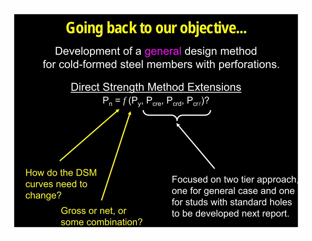
Going back to our objective...Development of a general design method

for cold-formed steel members with perforations.

Direct Strength Method ExtensionsPn = f (Py, Pcre, Pcrd, Pcrl)?

How do the DSMcurves need tochange?

Gross or net, or some combination?

Focused on two tier approach,one for general case and onefor studs with standard holesto be developed next report.

0 0.5 1 1.5 2 2.50

0.2

0.4

0.6

0.8

1

λc Pcre( )

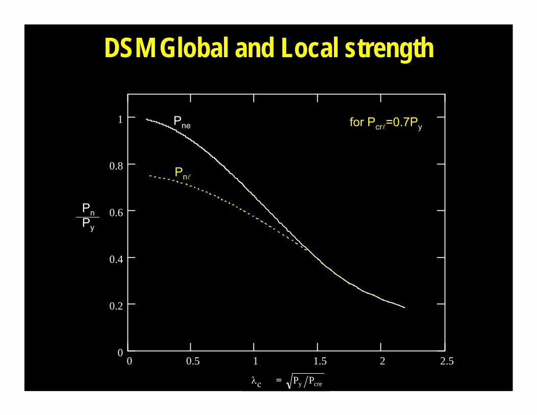
DSM Global and Local strength

for Pcrl=0.7Py

Pnl

Pne

PnPy

λc = crey PP

0 0.5 1 1.5 2 2.50

0.2

0.4

0.6

0.8

1

λc Pcre( )

DSM Global and Local Strength

for Pcrl=0.7Py

Pnl

Pne

PnPy

for 5.1c ≤λ

for λc > 1.5

λc = crey PP

crey2c

ne P877.0P877.0P =⎟⎟⎠

⎞⎜⎜⎝

⎛

λ=

Pne = yP658.02c ⎟⎠⎞⎜

⎝⎛ λ

0 0.5 1 1.5 2 2.50

0.2

0.4

0.6

0.8

1

λc Pcre( )

DSM Global and Local Strength

for Pcrl=0.7Py

Pnl

Pne

PnPy

for 5.1c ≤λ

for λc > 1.5

λc = crey PP

crey2c

ne P877.0P877.0P =⎟⎟⎠

⎞⎜⎜⎝

⎛

λ=

for λl 776.0≤ Pnl = Pne

for λl > 0.776 Pnl = ne

4.0

ne

cr4.0

ne

cr PPP

PP

15.01 ⎟⎟⎠

⎞⎜⎜⎝

⎛

⎥⎥

⎦

⎤

⎢⎢

⎣

⎡

⎟⎟⎠

⎞⎜⎜⎝

⎛− ll

λl = lcrne PP

Pne = yP658.02c ⎟⎠⎞⎜

⎝⎛ λ

Effect of using Pynet instead of Py

0 0.5 1 1.5 2 2.50

0.2

0.4

0.6

0.8

1

λc Pcre( )

for Pcrl=0.7PyPynet=0.7Py

Pnl

Pne

Pne-net: Pne if Pynet replaces Py

Pnl-net: Pnl if Pynet replaces Pyin the global and local curves

PnPy

λc = crey PP

Pynet=0.7Py

Cap the global curve at Pynet?

0 0.5 1 1.5 2 2.50

0.2

0.4

0.6

0.8

1

λc Pcre( )


Pnl

Pne

Pne-cap: Pne < Pynet

Pnl-ne-cap: Pnl if Pne < Pynet used

PnPy

λc = crey PP

0 0.5 1 1.5 2 2.50

0.2

0.4

0.6

0.8

1

λc Pcre( )

Or just cap the local curve only..


Pnl

Pne

Pnl-capPnl<Pynet.Pn

Py

λc = crey PP

Comparison of options

0 0.5 1 1.5 2 2.50

0.2

0.4

0.6

0.8

1

λc Pcre( )


Pnl-ne-cap

Pnl-ne-net

Pnl-cap

Pnl

Pne

PnPy

λc = crey PP

Closer look at stub columns

0 0.5 1 1.5 2 2.50

0.2

0.4

0.6

0.8

1

λc Pcre( )


Pnl-ne-cap

Pnl-ne-net

Pnl-cap

Pnl

Pne

PnPy

vary

stub column..

λc = crey PP

Local buckling strength for a stub column

0 0.5 1 1.5 2 2.5 3 3.50.3

0.4

0.5

0.6

0.7

0.8

0.9

1

1.1

( )

PnPne

for Pynet=0.7Py

Pnl-ne-cap

Pnl-ne-net

Pnl-cap

λl vary

Local buckling strength for a stub column

0 0.5 1 1.5 2 2.5 3 3.50.3

0.4

0.5

0.6

0.7

0.8

0.9

1

1.1

( )

PnPne

λl

for Pynet=0.7Py

Pnl-ne-cap

Pnl-ne-net

Pnl-cap

initial FE simulationsshow data here soalso considering atransition line as shown.(Pnl-transition)

Intermediate length column...

0 0.5 1 1.5 2 2.50

0.2

0.4

0.6

0.8

1

λc Pcre( )


Pnl-ne-cap

Pnl-ne-net

Pnl-cap

Pnl

Pne

PnPy

vary

intermediate lengthcolumn...

Local buckling strength

0 0.5 1 1.5 2 2.5 30.2

0.4

0.6

0.8

1

1.2

PnPne

λl

for Pynet=0.7Py

Pnl-ne-cap

Pnl-ne-net

Pnl-cap

0 2 4 6 8 10 12 14 16 180

5

10

15

20

25

30

35

L/H

spec

imen

cou

nt

Tests on columns with holesReference Author Publication Date Types of Specimens Cross Section End Conditions

1 Ortiz-Colberg 1981 Stub Column Long Column Lipped Channel

Fixed-Fixed Weak Axis Pinned

2 Pekoz and Miller 1987 Stub Column Lipped Channel Fixed-Fixed 3 Sivakumaran 1994 Stub Column Lipped Channel Fixed-Fixed 4 Abdel-Rahman 1998 Stub Column Lipped Channel Fixed-Fixed 5 Pu 1999 Stub Column Lipped Channel Fixed-Fixed 6 Moen and Schafer 2007 Intermediate Len. Lipped Channel Fixed-Fixed

see progress report 1 for full details of column databasesee progress report 3 and 4 for full details of Moen and Schafer tests

Normalized lengthof tested columnswith holes.. (priorto Moen and Schafertests)

* ** *

*Normalized lengthof Moen and Schafertested columns(2 ft and 4 ft tests)

Test-to-predicted ratios for columns with holes

average STDEV average STDEV average STDEV average STDEV1 use Py everywhere 1.03 0.11 1.09 0.16 1.14 0.11 0.84 0.082 use Pynet everywhere 1.17 0.08 1.23 0.13 1.27 0.10 1.04 0.123 cap Pne and Pnd 1.15 0.07 1.30 0.04* 1.16 0.10 1.03 0.114 cap Pnl and Pnd 1.07 0.08 1.15 0.10 1.16 0.10 1.01 0.115 transition Pnl and cap Pnd 1.06 0.08 1.15 0.10 1.16 0.10 1.03 0.11

Test-to-Predicted Ratio by Failure ModeDescriptionDSM

Option Local Distortional Global Yielding

0 0.5 1 1.5 2 2.5 30

0.5

1

1.5Option 1 - Py everywhere

λl=(Pne/Pcrl)

0.5

Pn/P

ne

DSM Local PredictionLocal Controlled TestDSM Yield ControlYield Controlled Test





DSM for Local buckling shown here

0 0.5 1 1.5 2 2.5 30

0.5

1

1.5Option 2 - Pynet everywhere

λl=(Pne/Pcrl)

0.5

Pn/P

ne







0 0.5 1 1.5 2 2.5 30

0.5

1

1.5Option 3 - cap Pne, Pnd

λl=(Pne/Pcrl)

0.5

Pn/P

ne







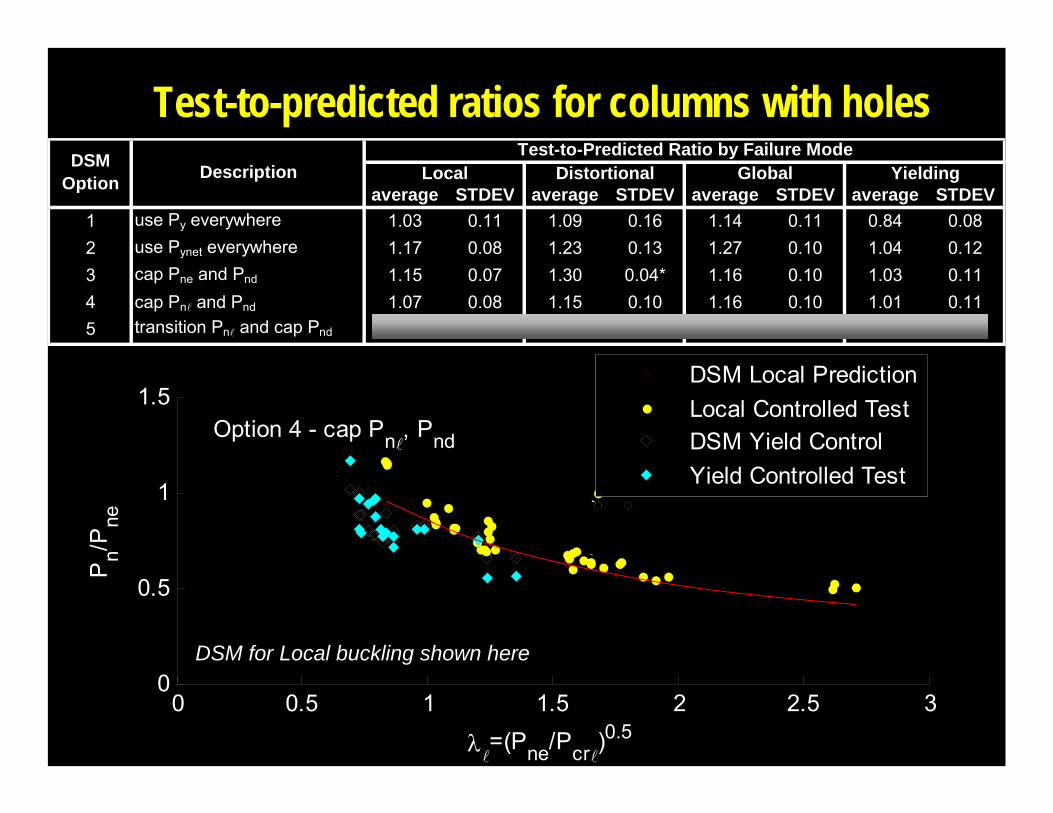
0 0.5 1 1.5 2 2.5 30

0.5

1

1.5Option 4 - cap Pnl, Pnd

λl=(Pne/Pcrl)

0.5

Pn/P

ne








0 0.5 1 1.5 2 2.5 30

0.5

1

1.5Option 5 - transition Pnl, cap Pnd

λl=(Pne/Pcrl)

0.5

Pn/P

ne







Conclusions• Past progress has established a good foundation for

completing a DSM method for members with holes– gathered test database of columns– gathered test database of beams– performed FEA eigenbuckling analysis of test data– completed new tests on columns with holes– initiated studies for simplified models of Pcr, Mcr which include the

influence of holes and will form the basis for a simplified method • Nonlinear FEA modeling

is advancing the state of the art for collapse modeling of CFS members with holes and provides a way to study details of DSM implementation

• DSM frameworkfor handling changes in elastic buckling and strength (net vs. gross) are now nearly complete – the changes are not drastic.

Future Work• Development of tiered approach for elastic

buckling (Pcrl, Pcrd, Pcre, Mcrl, Mcrd, Mcre) prediction– Simple methods for limited hole configurations– Guidance for general cases where

FEA eigenbuckling analysis must be used– Tools for automated evaluation of FEA eigenmodes

• Nonlinear FEA modeling to collapse for columns and beams with holes to augment experimental database

• Selection of final DSM expressions and reliability calculations

• Ballots and design aids

Supplementary slides

DSM and columns with holesFlexural, Torsional, or Torsional-Flexural Buckling The nominal axial strength, Pne, for flexural, … or torsional- flexural buckling is

for 5.1c ≤λ Pne = yP658.02c ⎟⎠⎞⎜

⎝⎛ λ

for λc > 1.5 crey2c

ne P877.0P877.0P =⎟⎟⎠

⎞⎜⎜⎝

⎛

λ=

where λc = crey PP

Py = AgFy Pcre= Critical elastic global column buckling load Ag = gross area of the column

Local Buckling The nominal axial strength, Pnl, for local buckling is

for λl 776.0≤ Pnl = Pne

for λl > 0.776 Pnl = ne

4.0

ne

cr4.0

ne

cr PPP

PP

15.01 ⎟⎟⎠

⎞⎜⎜⎝

⎛⎥⎥

⎦

⎤

⎢⎢

⎣

⎡⎟⎟⎠

⎞⎜⎜⎝

⎛− ll

where λl = lcrne PP Pcrl = Critical elastic local column buckling load Pne is defined above.

0. Pcr includes the hole

DSM Options...

1. Leave equations alone (except Pcr)

2. replace Py with Pyneteverywhere

3. Cap Pne to Pynet

4. Cap Pnl to Pynet

5. Cap Pnl to Pynet and add a transition portion to Pnl

0 0.5 1 1.5 2 2.5 30

0.5

1

1.5

λc=(Py/Pcre)0.5

Pn/P

y

Option 1 - Py everywhere

0 0.5 1 1.5 2 2.5 30

0.5

1

1.5

λcnet=(Pynet/Pcre)0.5

Pn/P

y

Option 2 - Pynet everywhere DSM Global Prediction

Global Controlled Test

0 0.5 1 1.5 2 2.5 30

0.5

1

1.5

λc=(Py/Pcre)0.5

Pn/P

y

Option 3 - cap Pne, Pnd

0 0.5 1 1.5 2 2.5 30

0.5

1

1.5

λc=(Py/Pcre)0.5

Pn/P

y

Option 4 - cap Pnl, Pnd

0 0.5 1 1.5 2 2.5 30

0.5

1

1.5

λc=(Py/Pcre)0.5

Pn/P

y

Option 5 - transition Pnl, cap Pnd

Global

0 0.5 1 1.5 2 2.5 30

0.5

1

1.5Option 1 - Py everywhere

λd=(Py/Pcrd)0.5

Pn/P

y

0 0.5 1 1.5 2 2.5 30

0.5

1

1.5Option 2 - Pynet everywhere

λdnet=(Pynet/Pcrd)0.5

Pn/P

y

DSM Dist. PredictionDist. Controlled TestDSM Yield ControlYield Controlled Test

0 0.5 1 1.5 2 2.5 30

0.5

1

1.5Option 3 - cap Pne, Pnd

λd=(Py/Pcrd)0.5

Pn/P

y

0 0.5 1 1.5 2 2.5 30

0.5

1

1.5Option 4 - cap Pnl

, Pnd

λd=(Py/Pcrd)0.5

Pn/P

y

0 0.5 1 1.5 2 2.5 30

0.5

1

1.5Option 5 - transition Pnl, cap Pnd

λd=(Py/Pcrd)0.5

Pn/P

y

Distortional

0 0.5 1 1.5 2 2.5 30

0.5

1

1.5


λd=(Py/Pcrd)0.5

Pte

st/P

n

0 0.5 1 1.5 2 2.5 30

0.5

1

1.5

Option 2 - Pynet everywhere

λdnet=(Pynet/Pcrd)0.5

Pte

st/P

n

Distortional ControlledYield Controlled

0 0.5 1 1.5 2 2.5 30

0.5

1

1.5


λd=(Py/Pcrd)0.5

Pte

st/P

n

0 0.5 1 1.5 2 2.5 30

0.5

1

1.5


λd=(Py/Pcrd)0.5

Pte

st/P

n

0 0.5 1 1.5 2 2.5 30

0.5

1

1.5


λd=(Py/Pcrd)0.5

Pte

st/P

n

distortional slen. vs. test-to-pred.

0 0.5 1 1.5 2 2.5 30

0.5

1

1.5


λl=(Pne/Pcrl

)0.5

Pte

st/P

n

0 0.5 1 1.5 2 2.5 30

0.5

1

1.5


λl=(Pne/Pcrl

)0.5

Pte

st/P

n

Local ControlledYield Controlled

0 0.5 1 1.5 2 2.5 30

0.5

1

1.5


λl=(Pne/Pcrl

)0.5

Pte

st/P

n

0 0.5 1 1.5 2 2.5 30

0.5

1

1.5


λl=(Pne/Pcrl

)0.5

Pte

st/P

n

0 0.5 1 1.5 2 2.5 30

0.5

1

1.5


λl=(Pne/Pcrl

)0.5

Pte

st/P

n

local slen. vs. test-to-pred.

0.5 0.6 0.7 0.8 0.9 10

0.5

1

1.5


Anet/Ag

Pte

st/P

n

0.5 0.6 0.7 0.8 0.9 10

0.5

1

1.5


Anet/Ag

Pte

st/P

n

Local ControlledYield Controlled

0.5 0.6 0.7 0.8 0.9 10

0.5

1

1.5


Anet/Ag

Pte

st/P

n

0.5 0.6 0.7 0.8 0.9 10

0.5

1

1.5


Anet/Ag

Pte

st/P

n

0.5 0.6 0.7 0.8 0.9 10

0.5

1

1.5


Anet/Ag

Pte

st/P

n

Anet/Ag vs. test-to-pred.

Global strength options

0 0.5 1 1.5 2 2.50

0.2

0.4

0.6

0.8

1

λc Pcre( )


PnPy

λc = crey PP

1

23

4 5

Local strength options

0 0.5 1 1.5 2 2.5 30.2

0.4

0.6

0.8

1

1.2

PnPne

λl

for Pynet=0.7Py

1

2

3

4 5

Direct Strength Design for Cold-Formed Steel Members with Perforations Holes Progress... ·...

Documents

Transcript of Direct Strength Design for Cold-Formed Steel Members with Perforations Holes Progress... ·...