Detecting Opportunistic Special Items

Detecting Opportunistic Special Items

Carol Anilowski Cain Assistant Professor of Accounting Winston-Salem State University

[email protected]

Kalin S. Kolev Associate Professor of Accounting

Baruch College - CUNY [email protected]

Sarah McVay

Professor of Accounting University of Washington

[email protected]

Management Science, Forthcoming

ABSTRACT

The frequency of special items has increased dramatically over time, offering a convenient conduit for the inappropriate classification of past, present, and future recurring expenses as non-recurring. Identifying this misclassification is especially important in light of the pervasive use of non-GAAP earnings in recent periods, as special items offer camouflage for excluded recurring expenses. Building on prior research, we propose a method for identifying the predicted level of special items, attributing any excess to opportunism, and demonstrate the importance of this partitioning for financial statement users. In particular, we provide evidence that the opportunistic portion of special items is associated with lower future earnings, cash flows, and returns. We conclude that this portion of special items is more likely to contain opportunistically misclassified recurring expenses that should have been recognized as such in prior, current, or future periods. Thus, we provide a meaningful partition of special items that should be useful to investors, analysts, creditors, auditors, and regulators, as each of these parties must assess the implications of special items. Keywords: Special items; transitory items; non-GAAP earnings; earnings quality; earnings

management. We appreciate the comments and suggestions of two anonymous reviewers, an anonymous associate editor, Suraj Srinivasan (the managing editor), Mary Billings (FARS discussant), Asher Curtis, Weili Ge, Michelle Hanlon, Doug Hanna, Eddie Riedl, Edgar Rodriguez Vazquez, Doug Skinner, Mike Willenborg, Benjamin Whipple, and workshop participants at London Business School, the University of Arizona, the University of Connecticut, Rutgers University, Yale School of Management, and the FARS midyear conference. An earlier version of this paper was entitled “Qualifying Special Items: An Identification and Examination of Lower-Quality versus Higher-Quality Income-Decreasing Special Items.”

1

1. Introduction

The reporting of special items has increased dramatically over time (Elliott and Hanna

1996; Collins et al. 1997; Donelson et al. 2011) with 50 percent of US publicly traded firms

reporting income-decreasing special items by 2016 (Figure 1).1 The designation of special items

as unusual or infrequent is important because it highlights that management expects these

charges to be more transitory than recurring expenses (e.g., Lipe 1986; Fairfield et al. 1996). It

naturally follows that investors, analysts, and compensation committees typically place less

weight on special items than on core earnings (e.g., Elliott and Shaw 1988; Philbrick and Ricks

1991; Dechow et al. 1994; Elliott and Hanna 1996; Gaver and Gaver 1998).

Although the increase in special items largely reflects changes in the economic and

regulatory landscape (e.g., Collins et al. 1997; Donelson et al. 2011), it also heightens concerns

about the use of special items to manage earnings (e.g., Riedl 2004; Kolev et al. 2008; Cready et

al. 2010). In particular, management can misclassify past, present, and future recurring expenses

as a current period special item (Barton and Simko 2002; Burgstahler et al. 2002; Riedl 2004;

McVay 2006; see examples in Appendix 1). Assessing the composition of special items is

particularly important considering the increasing prevalence of “non-GAAP” earnings, with

approximately 50 percent of firms reporting non-GAAP earnings by 2013 (see Figure 2 of

Bentley et al. 2018). Non-GAAP earnings are more value-relevant than GAAP earnings, which is

often attributed to the removal of special items (e.g., Bradshaw and Sloan 2002; Lougee and

Marquardt 2004).

1 The term “special items” refers to unusual or infrequent items that are reported as a separate component of income from continuing operations, and the nature and financial effects of each event or transaction is disclosed on the face of the income statement or in the notes to the financial statements (APB 30; ASC 225-20-45-16). We focus on income-decreasing special items as we expect misclassified recurring expenses to make the income-decreasing special item larger, whereas the predictions for income-increasing special items are more nuanced. We expand on these subtleties in later discussions.

2

A practical tool for assessing the validity of reported special items is therefore necessary

to evaluate the quality of a firm’s financial reports. We fill this void by proposing a methodology

to predict economically driven special items, the excess of which likely contains

opportunistically misclassified recurring expenses from the past, present, and future—hereafter

“opportunistic special items.” Such a tool is particularly important given the prevalence of non-

GAAP earnings. Although academic studies of special items are rife with concerns of

manipulation (Barton and Simko 2002; Burgstahler et al. 2002; Atiase et al. 2004; Riedl 2004;

McVay 2006; Kolev et al. 2008; and Bens and Johnston 2009, among others), the non-GAAP

earnings literature generally treats excluded special items as relatively “safe.” Instead, that

literature focuses on other exclusions, such as the exclusion of amortization expense, and more

recently, stock based compensation expense, as the vehicle for financial reporting manipulation

involving non-GAAP earnings (e.g., Doyle et al. 2003; Black and Christensen 2009; Doyle et al.

2013). By partitioning the predicted and opportunistic components of special items, we are able

to bridge these two distinct, but clearly related, streams of literature.

Although the type and frequency of specific special items are important to financial

statement users, alone these identifiers are insufficient to classify a given special item as

opportunistic. A single special item could contain both recurring and transitory expenses (e.g.,

Borden and Enterasys Networks—both examples in Appendix 1—had actual restructuring

charges which contained some misclassified recurring expenses and hence were overstated).

To form an estimate of the economically driven “predicted” component of special items,

we build on evidence in prior research on the determinants of special item reporting (e.g., Francis

et al. 1996; Riedl 2004; Bens and Johnston 2009; Cready et al. 2010). Specifically, we use a

Tobit estimator to jointly model the propensity of reporting income-decreasing special items

3

during a specific year and the magnitude of the charge, inferring the predicted (opportunistic)

special item portion as the resultant fitted value (residual). To validate our partition, we examine

the association of the special items partitions with future firm performance. We find that our

estimate of opportunistic special items is significantly negatively associated with both future

earnings and cash flows, on average, whereas predicted special items are not, supporting that our

identification of opportunistic special items contains misclassified recurring expenses. Our

model, however, could classify less transitory (but still special) expenses as opportunistic. To

address this concern, we also examine future abnormal stock returns. We find that opportunistic

special items are significantly negatively associated with future abnormal returns, whereas the

association is insignificant for predicted special items. In short, these analyses support that our

model of special items allows users to isolate the economically driven component of special

items, which behave in a manner that is more consistent with the concept of a transitory item

(Ohlson 1999).

As additional analyses, we document that our estimate of opportunistic special items are

associated with future restatements related to special items (i.e., items first classified as special

are restated to recurring expenses) and also document that the probability of just meeting or

beating the analysts’ consensus forecast is higher when the proportion of opportunistic special

items, relative to total special items, is higher. Collectively, we interpret these results as further

evidence that we are able to identify some misclassified recurring expenses from the past,

present, and future.

The literature on special items is vast. Extant research, however, focuses on either

specific types, such as impairments or restructuring charges (Francis et al. 1996; Moehrle 2002;

Atiase et al. 2004; Riedl 2004; Bens and Johnston 2009; Lee 2014), total special items (Doyle et

4

al. 2003), the sign of special items (Kinney and Trezevant 1997; Riedl and Srinivasan 2010), or

the recurrence of special items (Elliott and Hanna 1996; Cready et al. 2010). In contrast, we

propose a systematic approach to assess the validity of income-decreasing special items, with the

goal of separating the economically driven, valid, component from the portion more likely to

reflect strategic financial reporting.

This partition should be useful to a number of parties interested in assessing the merit of

managers’ special item designations, as it is extremely difficult to gauge the reasonableness of

many special items, such as restructuring charges, especially relying solely on external reports.

One example is regulators, who need to decide whether to allow separate reporting of special

items. Another is investors and analysts who need to assess the quality of non-GAAP earnings, a

central performance indicator that has reached all-time highs in terms of usage (e.g., Bentley et

al. 2018) and has again come under SEC scrutiny (Michaels and Rapoport 2016). In addition, our

partitioning should also be of interest to auditors, who often waive proposed classification

adjustments (Nelson et al. 2002), and due diligence teams valuing target firms for M&A

purposes (Skaife and Wangerin 2013). Identifying potentially opportunistic special items also

allows financial statement users to more carefully scrutinize prior and future earnings, which

would be overstated if recurring expenses from the past and future are shifted into current period

special items.

We expect our relatively simple model, which does not require forward-looking

information and is relatively easy to implement, to be useful to financial statement users who

must assess the implications of special items in real time. As with all regression-based

partitioning models, however, our approach has limitations. Most notably, this approach yields a

relatively large residual which contains some economically driven special items—it overstates

5

opportunistic special items. Moreover, it does not identify the period from which the recurring

expenses are shifted (i.e., the past, present, or future). As a step to resolving these issues, we

develop explicit estimates of shifting from the past, present, and future, which may be of greater

interest to academics or regulators wishing to assess, ex post, the quality of prior special items.

The estimate of opportunistic special items using this more arduous methodology provides a

lower-bound estimate of opportunistic special items, and suggests that misclassified recurring

expenses make up approximately one-third of special items, on average.

2. Motivation

The components of the income statement are intended to provide information about the

underlying economics of a firm’s transactions. Fairfield et al. (1996) offer evidence that the

persistence of earnings components is generally declining as one moves down the income

statement. They find that, on average, core earnings are more than five times as persistent as

special items. For example, when forecasting future return-on-equity (their Table 2), the

estimated coefficient on special items is 0.123, whereas the coefficient on gross margin is 0.636.

This lower persistence of special items is reasonable considering the types of charges comprising

special items: e.g., restructuring charges, asset write-offs, and gains or losses on the sale of

assets. Consistent with this notion, investors, analysts, and compensation committees generally

discount income-decreasing special items, largely excluding them from GAAP earnings in

assessing firm performance or determining managerial compensation (e.g., Elliott and Shaw

1988; Philbrick and Ricks 1991; Dechow et al. 1994; Elliott and Hanna 1996; Gaver and Gaver

1998; Bradshaw and Sloan 2002; Bentley et al. 2018).

This differential treatment makes special items a convenient tool for managing earnings

(e.g., Elliott and Shaw 1988; Kinney and Trezevant 1997; Burgstahler et al. 2002; Moehrle 2002;

6

McVay 2006; Bens and Johnston 2009). For example, managers can under-report past expenses,

such as depreciation (e.g., by using too large of a residual value or too long of an expected life)

which bloats the balance sheet (Barton and Simko 2002; Hirshleifer et al. 2004), and can

ultimately be written off as a special item. Thus, managers might view the deceleration of

expenses as a low-cost means to manage reported earnings if they plan to write off the

accumulated expenses as a special item in a future period. This tactic is especially attractive

since the subsequent write-down is typically excluded from non-GAAP earnings, which are the

focus of investors and analysts. In other words, the benefit is more than just a timing difference,

as the “reversal” of the accrual build-up is discounted by investors.

Managers can also manipulate the classification of expenses within the income statement.

McVay (2006) documents that managers misclassify core operating expenses as special items in

order to inflate core earnings (see also Fan et al. 2010). Moreover, Robinson (2010) documents

managers are willing to incur real costs to classify charges as tax expenses rather than operating

expenses. These studies support the notion that managers care about the classification of

expenses within the income statement.2 Shifting operating expenses to special items allows

managers to report better core performance without changing bottom-line earnings, which may

be perceived as beneficial in that analysts, investors, and compensation committees tend to

discount the special items, focusing on core earnings. Indeed, McVay (2006) provides some

evidence that investors are negatively surprised when these misclassified core expenses recur in

future periods.

2 Kinney and Trezevant (1997) find that managers tend to break out transitory expenses on the face of the income statement, while merely disclosing transitory gains in the footnotes, although Riedl and Srinivasan (2010) suggest that this disclosure choice corresponds to the permanency of the special items. Rather than examine where the special items are reported, we analyze the association of our measure of opportunistic special items with future returns and restatements to corroborate that we identify misclassified expenses, rather than relatively more permanent (but appropriately classified) special items.

7

Finally, managers may shift future recurring expenses into the current period special

item, thereby artificially improving future earnings. Specifically, managers have been accused of

engaging in big bath accounting (Moore 1973; Healy 1985; Murphy and Zimmerman 1993;

Pourciau 1993; Kirschenheiter and Melumad 2002; Atiase et al. 2004; Bens and Johnston 2009)

to improve future earnings; and, the time-series properties of special items support this

conjecture (Levitt 1998; Burgstahler et al. 2002; Fairfield et al. 2009; Cready et al. 2010).3 Thus,

special items can contain future expenses, in which case special items will be associated with

future unexpected improvements in earnings (e.g., Burgstahler et al. 2002; Atiase et al. 2004;

Dechow and Ge 2006). For example, although Atiase et al. (2004) find that firms with losses and

multiple restructuring charges tend to improve in the following years, they note that the

improvement is more pronounced in earnings than in cash flows, and caveat that they cannot rule

out earnings management.4

Disentangling the recurring component of special items is difficult for financial statement

users, as they generally do not have sufficient information to identify how much of a specific

expense represents appropriately classified special items versus misclassified recurring

expenses.5 Referring to the examples in Appendix 1, if an auditor failed to identify and correct

such misreporting, is it reasonable to expect a firm outsider to discern shifting at the time of the

reporting of the special item?

3 Managers have also been found to create reserves that are later reversed into income, allowing them to meet future benchmarks (Moehrle 2002). These reversals should be classified as future income-increasing special items, whereas our model of shifting from the future focuses on future earnings before special items. Thus, our analysis does not encompass this earnings management technique. 4 Our residual-based estimate of opportunistic special items encapsulates shifting from the past, present, and future. The inclusion of shifting from the future, however, biases against finding negative future outcomes, as the mechanism leads to higher future earnings and stock returns (Burgstahler et al. 2002). 5 Although in earlier periods the recurrence of special items allowed for a relatively strong indicator of perceived quality (e.g., Elliott and Hanna 1996; Cready et al. 2010), we expect the usefulness of recurrence as a signal of opportunism to decline, as the appropriate application of recent financial standards results in multi-period special items (e.g., SFAS 146, now ASC 420; Lee 2014). As a practical matter, we confirm that our partitioning notably outperforms an analogous partition that treats repeated special items as opportunistic (untabulated).

8

Considering the feasibility of using special items as a vehicle for managing earnings, a

natural question becomes why we observe other, much costlier, types of earnings management.

First, firms do not report special items every period. Thus, we posit that opportunistic managers

typically capitalize on the existence of a valid special item, using it as camouflage. Second, the

valuation and compensation benefits to reporting special items decline as this practice increases

in frequency (Elliott and Hanna 1996; Cready et al. 2010). Specifically, as special items recur,

financial statement users begin treating them more like recurring earnings. This imposes a

natural constraint on how frequently managers can shift past, present, and future expenses into

special items.

Even potentially contaminated by the inclusion of past, present, and future recurring

expenses, special items remain more transitory than core earnings on average. The inclusion of

these recurring expenses, however, reduces the usefulness of the separation of special items from

core earnings and evidence supports that current period special items are predictive of both

future special items (Francis et al. 1996; Cready et al. 2010) and future core earnings

(Burgstahler et al. 2002; McVay 2006; Fairfield et al. 2009; Cready et al. 2010). In sum, we

believe that a meaningful assessment of the composition of reported special items would be

useful to virtually all financial statement users.

The approach we take focuses on modeling economically motivated special items and

treating any income-decreasing special items exceeding this predicted magnitude as

opportunistic—likely to contain past, present, and future recurring expenses. Similar to other

attempts to partition accounting variables (e.g., identifying discretionary accruals), the

methodology we propose trades off feasibility and precision. We conduct a number of tests to

verify that the partitioning is meaningful. We first explore whether predicted and opportunistic

9

special items are differentially associated with future earnings (before special items) and

operating cash flows. This analysis is motivated by the notion that recurring expenses,

misclassified as transitory, will be negatively associated with future earnings and operating cash

flows as they recur (Doyle et al. 2003; Kolev et al. 2008).

Clearly, there is natural variation in the permanence of special items that does not reflect

opportunism (e.g., Riedl and Srinivasan 2010). Thus, it is possible that the residual of our model

contains less transitory, but still appropriately classified, special items. In this case, these

expenses would be associated with future earnings and cash flows, but not reflective of

intentional misclassification of recurring expenses from the past, present, and future. This

argument does not extend to the association between future abnormal stock returns and special

items, which we view as clearer evidence that recurring expenses are misclassified as transitory.

Specifically, if investors learn of the misclassification over time as the expenses recur,

opportunistic special items should be negatively associated with future returns. Investors could

also learn of the misclassification if special items are subsequently restated as recurring

expenses, yielding a similar prediction. In support of the latter mechanism, we provide several

examples of restatements related to the shifting of expenses from the past, present, and future

(Appendix 1). For example, in 1992 Borden misclassified concurrent recurring expenses (largely

marketing expenses) as one-time charges and was subject to an SEC enforcement action, and in

1996, Sunbeam took a big-bath by writing off future expenses, also attracting the attention of the

SEC—both resulted in a restatement. Thus, we expect that the misclassification of recurring

expenses as special items should lead to lower future abnormal stock returns, as investors see

“transitory” expenses recur.

10

In summary, we predict economically driven special items and attribute any excess to

opportunism. We expect the opportunistic, but not predicted, component will be negatively

associated with future earnings, cash flows, and returns. As additional analyses, we explore

directly whether opportunistic special items are associated with a higher likelihood of subsequent

financial statement restatements or linked to reporting incentives via the likelihood of meeting or

narrowly beating the analysts’ consensus forecast.

3. Sample Selection, Descriptive Statistics and Measurement of Shifting

3.1 Sample Selection

We obtain financial and market data from Compustat, accounting restatements data from

Audit Analytics, equity returns from CRSP, and analysts’ forecast error data from IBES. The

sample spans 1989 through 2016. We begin the sample in 1989, as we require lagged data from

the statement of cash flows. Since some analyses require subsequent data (e.g., future earnings,

cash flows, and returns), the time series length varies across specifications. The number of

observations varies across tests due to data availability. We scale all continuous financial

variables, other than CFO Volatility and Operating Cycle, by Net Sales (Compustat item SALE).

We do not consider assets, book value of equity, or market value of equity as scalars since assets

and book value of equity are affected by the accumulation of past expenses and the acceleration

of future expenses, and market performance is an important predictor of special items. In other

words, any of the three deflators is likely to bias the analysis, whereas we have no reason to

believe that sales would similarly bias the estimates. We exclude firm-year observations with

less than one million in sales to mitigate potential small-denominator problems. We also exclude

firm-year observations with a change in fiscal-year end. All continuous variables are winsorized

at 1 percent and 99 percent by fiscal year to mitigate the influence of outliers. In addition, we

require each industry-year group to have at least 50 observations with non-missing data for the

11

model of economically driven special items, where the industry definition is based on the Fama

and French (1997) classification. The full sample comprises 104,495 firm-year observations for

11,991 individual companies.

3.2 Descriptive Statistics

The descriptive statistics for our main variables are presented in Panel A of Table 1; we

define the variables in Appendix 2. Mean total assets are approximately $6.8 billion, and mean

sales are approximately $2.9 billion. We obtain special items (SI) from Compustat; for ease of

interpretation, we multiply the variable by negative one, resulting in positive values representing

income-decreasing special items. Since the focus of the study is the potential shifting of expenses

into special items, we examine only the income-decreasing special items and set the income-

increasing special items to zero.6 Income-decreasing special items as a percentage of sales has a

mean of 2.44 and a median of zero.

In Panel B of Table 1 we partition the sample into firm-years with zero or income-

increasing special items and firm-years with income-decreasing special items. Firms reporting

income-decreasing special items tend to be larger, less profitable and have lower sales growth.

We include a correlation table in our online appendix.

6 Hypothetically, managers could also use income-increasing special items to inflate core earnings, i.e., record the transactions as “recurring.” If the tactic were successful, however, the special items in Compustat would be recorded as zero. Because we cannot rely on the same variables and models to identify earnings management using income-increasing special items, we opt to set income-increasing special items to zero. To maximize the sample size, we also set missing values for the special items variable to zero. Prior to setting income-increasing special items to zero, 13.9 percent of the sample had a net income-increasing special item, as reported by Compustat. The mean (median) magnitude of these income-increasing special items is $84.7 ($3) million, or 12.6 (0.9) percent of net sales (unwinsorized; not tabulated). Results are not sensitive to the removal of firm-year observations with income-increasing or missing special items (not tabulated).

12

4. Tests

4.1 Identifying Predicted and Opportunistic Special Items

Much of prior research on the determinants of special items focuses on specific types,

such as asset write-offs (Francis et al. 1996; Riedl 2004) and restructuring charges (Bens and

Johnston 2009; Lee 2014). These papers often consider both economic determinants and

incentives to report special items. We consider only the variables motivated as economic drivers,

as we expect incentives drive opportunistic special items. We model the economically driven

component of income-decreasing special items as follows:

SIi,t η λ Returnsi,t‐1 λ Returnsi,t‐3,t‐1 3∆ i,t‐3,t‐1 4∆ i,t‐3,t‐1 5Mergeri,t,t‐1 i,t‐1,t DiscontinuedOpi,t i,t ∆ i,t‐3,t‐1 i,t i,t‐3,t‐1 ∆ i,t i,t‐1 i,t‐1 i,t‐1 ln i,t‐1 μ ,

(1)

We identify the economically driven (opportunistic) component of income-decreasing

special items, PredSI (OppSI), as the fitted value (error term).7 We estimate Equation (1) as a

Tobit regression. We do so for two reasons. First, our construct of special items is censored

below at zero, with positive values reflecting income-decreasing special items. Second, reported

special items stem from a two-step process: managers first determine whether an unusual or

infrequent event has occurred during the period, and then assess the dollar amount to recognize

as a separate component of income from continuing operations.8 Since the Tobit estimator nests

an assessment of the observed magnitude of the dependent variable within a binary model

7 To address instances of delayed reporting of income-decreasing special items and the fact that Compustat item SPI combines income-increasing and income-decreasing special items, reporting the net effect, we apply two filters to the model estimates. First, we set PredSI and OppSI to zero if the variables are non-zero, but the firm does not report an income-decreasing SI for the period (7.15 percent of the observations). Second, if the firm reports income-decreasing special items, but the error term in the model is negative, we set OppSI to zero (8.46 percent of the observations). 8 Typically, we expect that the choice to misclassify recurring expenses as transitory is conditional on the opportunity. With a restructuring charge comes the opportunity to write off assets that had been previously over-stated through under-expensing, shift current recurring expenses to the charge, and write off unimpaired assets to lower future expenses. Asset write-offs, however, could also feasibly manifest as stand-alone removals of prior intentional deceleration of expenses.

13

predicting the existence of the variable, it is well-suited for our setting (see Riedl 2004 and Lee

2014 for similar applications).

We estimate the regressions by industry-year to control for industry-specific and

macroeconomic factors; to allow sufficient degrees of freedom, we require each industry-year

subsample to have at least 50 observations with non-missing data for each variable. This also

allows the estimated coefficients on the determinants to vary across industries and time; this is

especially important in our setting as prior research finds that the impact of economic

determinants has changed over time (e.g., Riedl 2004) and that pooled regressions do not provide

as good of a fit when predicting special items (e.g., Bens and Johnston 2009).

Turning to the model variables, following Francis et al. (1996), we include prior stock

returns, change in the book-to-market ratio, and change in return-on-assets.9 Following Donelson

et al. (2011), we include three indicator variables for economic events that could lead to special

items: a decline in employees from year t–1 to t, M&A activity in year t or t–1, and discontinued

operations in year t.10 Building on the models in Cready et al. (2010), Donelson et al. (2011), and

Riedl (2004), we also include large sales declines, change in sales, current period operating loss,

intensity of operating losses over the prior three years, and change in operating cash flows to the

vector of economic determinants. We conjecture that firms with longer operating cycles and

larger recognized tangible and intangible assets are at greater risk of recognizing income

decreasing special items, as each of these increases the need for estimates and, thus, the

9 Because we estimate this model by industry-year, we do not industry-adjust the book-to-market ratio, and we do not include the change in industry return-on-assets or book-to-market ratio. For the same reason, we do not include change in GDP (e.g., Riedl 2004). Also, although Francis et al. (1996) use five-year changes for many of their variables, we only consider three-year changes to maximize the number of observations. 10 Donelson et al. (2011) consider M&A activity in year t only, but we also include t–1 as we expect some integration expenses to flow into the year after the M&A transaction, especially if the deal closes late in the fiscal year. Clearly some of these economic determinants could capture incentives to shift. For example, M&A transactions lead to economically driven M&A expenses, but also may correlate with the desire to present higher earnings.

14

likelihood of write-downs. Therefore, we include the length of a firm’s operating cycle and its

capital and intangible intensities. Finally, following Francis et al. (1996) and Cready et al.

(2010), we include a measure of firm size.

In Table 2 we present summary results from the 771 industry-year Tobit estimations of

Equation (1). The first and second columns present the mean and median industry-year

regression coefficients, and the second two columns present the percent of the estimated

coefficients that obtain the predicted sign and are significant in the predicted direction (one-

tailed test; p < 0.10), respectively. For example, 83.9 percent of the industry-year regressions

yield a positive coefficient on loss in year t and the effect is significant in 57.1 percent of the

cases.

Turning to the estimates, lagged returns are inversely related to special items, consistent

with special item firms generally experiencing poor performance prior to recognizing the

charges. Similarly, firms with increasing book-to-market ratios, as well as companies with

declining return-on-assets ratios, tend to have larger special items. Mergers tend to result in

special items (with merger and acquisition fees and in-process R&D both typically classified as

special items during the sample period), as do declines in employees and, at the median,

discontinued operations, consistent with these firms undergoing a business reconfiguration that

could lead to restructuring charges or asset impairments. Poorly performing firms (those with

losses, and declining sales and cash from operations) tend to have larger special items, as do

firms with longer operating cycles, consistent with longer operating cycles leading to greater

uncertainty, and thus, estimation errors (Dechow and Dichev 2002). Firms with more assets to

impair (tangible or intangible) also have larger special items. Finally, firm size is positively

15

associated with special items, consistent with prior work (e.g., Francis et al. 1996; Cready et al.

2010).

4.2 Test Results

4.2.1 Future Earnings, Cash Flows, and Equity Returns Realizations

To investigate the association between special items and future earnings, cash flows, and

equity returns, we estimate variations of the following regression model:

∑ ϕ φ1 i,t φ2 θ'FE , (2)

We cumulate the dependent variables (earnings, cash flows or returns) over the second and third

year after the observation date to avoid mechanical associations; the vast majority of cash

outflows related to liabilities established as part of the special item in year t take place in years t

and t+1 (e.g., severance fees within restructuring charges that are correctly paid to the employees

the current and subsequent year). Our intent is to capture expenses that continue to occur into the

future, rather than cash outflows related to liabilities associated with predicted special items.11

As before, SI is a continuous variable, defined as income-decreasing special items scaled

by sales, bound below at zero. In the specifications analyzing predicted and opportunistic special

items, we substitute SI for PredSI and OppSI. We estimate the models using Ordinary Least

Squares, clustering the errors at the firm level. Each model includes industry-year fixed effects,

FE, to absorb macroeconomic factors.

We consider three samples: 1) all observations with available data for the analysis (full

sample), 2) only firms that report income-decreasing special items in year t (SI sample), and 3)

only firms with opportunistic special items in year t (OppSI sample). Although the full sample

11 Results are similar if we include year t+1 in the measurement window or restrict the analysis to year t+1 (see the online appendix). As a technical point, to avoid survivorship bias, we retain observations with at least one data point in t+2 or t+3. That is, if data for t+3 are missing, the dependent variable is not coded as missing, but takes on the value of t+2. Requiring data for all years does not affect the inferences (not tabulated).

16

results allow a comparison to extant research, we view the SI and OppSI samples as more

informative since our focus is the effects of predicted and opportunistic special items, which, by

construction, are only present in firms that report special items during the year.

We report the regression results in Tables 3–5. We first consider future earnings.

∑ denotes Net Income before Taxes and Special Items (Compustat item PI, adjusted

for the Compustat-reported income-decreasing special items), scaled by contemporaneous Net

Sales and cumulated over years t+2 and t+3. We focus on earnings before special items to avoid

a mechanical relation between current period special items and future period special items (e.g.,

Francis et al. 1996). Thus, any recurrence of special items should bias against finding evidence

of opportunism in our earnings estimations, as shifting future expenses to future special items

will increase future recurring earnings. We use pre-tax income to accommodate that Compustat

item SPI, which underlies our measure of income-decreasing special items, is reported pre-tax.

Turning to Table 3, we note that in the full sample, special items are not associated with

future earnings (t-statistic = 0.12). This non-result is consistent with findings in Doyle et al.

(2003) and Fairfield et al. (2009). When we examine firm-years with income-decreasing special

items, however, on average special items are negatively associated with future earnings (φ1 –

0.125; t-statistic = –1.98), and this coefficient appears slightly higher in the OppSI sample

(φ1 –0.132; t-statistic = –2.02).

When we examine the special items components, however, the results differ notably

between predicted and opportunistic special items. Specifically, predicted special items are

positively associated with future earnings in all three samples, consistent with operational

improvements resulting, for example, from efficiency gains related to a restructuring charge

(e.g., Atiase et al. 2004), whereas the estimated coefficients on opportunistic special items are

17

negative across the board, which is consistent with the recurrence of core expenses. An F-test

rejects the null of equivalence between the estimated coefficients on PredSI and OppSI for each

of the samples.

Although opportunistic special items are negatively associated with future earnings, the

absolute value of the coefficient is smaller than the coefficient on earnings before taxes and

special items (e.g., 0.356 < 1.016 in the sample with opportunistic special items) in each of the

samples; F-test not tabulated. This is not surprising considering the noise in the measurement of

opportunistic special items. As we note earlier, we do not expect that all of the special items in

that category are, in fact, misclassified recurring expenses. Instead, this partition allows for a

coarse categorization, isolating the highest-quality special items and documenting the notably

different implications of the two categories. When we form the more precise estimate of

opportunistic special items (we discuss the methodology in Section 4.3 and the online appendix),

the respective coefficient nearly doubles to 0.668 in absolute value (not tabulated). In other

words, one dollar of opportunistic special items is associated with lower earnings of 67 cents in

years t+2 and t+3. Although it remains smaller than the estimated coefficient on earnings before

taxes and special items, we view the effect as economically significant. In sum, we provide

evidence that the opportunistic, but not predicted, component of special items has negative

implications for future earnings.

We examine future cash flows in Table 4. ∑ denotes Cash from Operations

(Compustat item OANCF – XIDOC), scaled by contemporaneous Net Sales and cumulated over

years t+2 and t+3. Although the coefficient on total special items is not significant at

conventional levels for the full sample (t-statistic = –1.27), the association between special items

18

and future cash flows is significantly negative in the SI and OppSI samples.12 We again find that

this negative association is concentrated in the component of special items we classify as

opportunistic. Specifically, the estimated coefficients imply that on average, one dollar of

opportunistic special items during the current period corresponds to net operating cash outflows

in years t+2 and t+3 of 25 cents (OppSI sample). This amount is lower than the analogous

coefficient in Table 3 of 0.36 because some of the shifting is through depreciation expense,

which does not affect cash from operations.

Although the evidence in Tables 3 and 4 supports that the opportunistic component of

special items has different implications for future earnings and cash flows than the predicted

component, it is possible that the estimated coefficients capture natural variation in the

permanence of appropriately classified special items (e.g., Riedl and Srinivasan 2010). Thus, we

also examine future returns, which we do not expect to be systematically associated with

appropriately classified special items.

Turning to Table 5, ∑ denotes cumulative market-adjusted abnormal returns

for years t+2 and t+3, aggregated starting twelve months after the earnings announcement for

year t. The estimated coefficient on special items is significantly negative in all three samples.

When we partition special items into the predicted and opportunistic components, the effect is

again concentrated in opportunistic special items. In particular, the estimated coefficient on

predicted special items is insignificant, whereas the coefficients on opportunistic special items

are significantly negatively associated with future abnormal returns across all three samples,

consistent with investors’ disappointment as shifted expenses recur. For example, in the full

sample the estimated coefficient on opportunistic special items is –0.240 versus –0.091 for

12 Note that Doyle et al. (2003) do not consider firms with non-zero special items. The insignificant coefficient on special items for the full sample is consistent with the results presented in their Table 3, Panel B.

19

predicted special items. Even though an F-test fails to reject the null of equivalence, the

difference in the magnitude of the estimated coefficients is notable. Turning to economic

significance, for the full sample a one standard deviation increase in opportunistic special items

implies negative abnormal returns in years t+2 and t+3 of –0.240 × 0.0580 = –1.39 percent. A

similar analysis indicates that a one standard deviation increase in predicted special items implies

negative abnormal returns in years t+2 and t+3 of –0.091 × 0.0391 = –0.36 percent.

The estimated coefficients on the control variables are generally consistent with

expectations: Momentum and Size are negative, while BM is positive (e.g., Carhart 1997; Fama

and French 1992). Beta is statistically insignificant across specifications, which conflicts with

theory, but aligns with extant empirical research (Fama and French 1992). The one exception is

the accruals metric we use, AccrualsPre-SI, which is not negative and significant. This is likely

because accruals and special items are highly correlated, and much of the “accrual” anomaly is

due to special items (Dechow and Ge 2006). Because we cannot separate special items between

accruals and cash flows, we remove total special items from the accrual variable. Although we

realize the assumption that special items are entirely accruals is not realistic, as a practical

matter, if this design choice was simply a re-allocation of accruals into special items, we would

expect both predicted and opportunistic special items to be negatively associated with future

abnormal returns, which is not the case.

In summary, the results in Tables 3–5 support that the implications of special items for

future earnings, cash flows, and equity returns depend on the validity of the special item. In other

words, it validates the notion that special items should not be treated as a homogenous group and

highlights the importance to investors of exercising due diligence in assessing how much of the

reported special items should be considered transitory, thereby increasing the usefulness of non-

20

GAAP earnings. Although the returns tests provide some confidence that our classification of

opportunistic special items includes misclassified recurring expenses, we proceed by

corroborating the meaningfulness of our partition with an analysis of subsequent restatements

related to special items, as well as an examination of incentives to shift in the next section.

4.2.2. Additional Analysis

In this section we provide two supplemental analyses. We first examine whether the

propensity to experience a subsequent restatement related to special items in year t increases with

the opportunistic component of the special items. Then, we evaluate whether our estimate of

opportunistic special items is related to incentives to shift, using the propensity to meet or just

beat the analyst forecast as the setting.

4.2.2.1. Future Restatements

As we note previously, Appendix 1 offers several anecdotal examples of restatements

related to the intentional misclassification of recurring expenses. Here we investigate the issue in

a systematic manner by exploring the association between the special items partitions and

subsequent financial restatements. Specifically, we estimate the following regression model:

Pr 1 F ϕ φ1 i,t φ2ln ATi,t φ3SalesVoli,t φ CFOVoli,t φ %Lossi,t φ BigNi,t φ OperatingCyclei,t φ ∆SalesGrowthi,t φ9Returnsi,t θ'FE ,

(3)

Ideally, Restate would take the value of one if a recurring expense is misclassified as

special and later restated. In practice, however, it is very difficult to identify restatements related

specifically to the misclassification of special items; not only are these relatively rare, but

traditional data providers, such as Audit Analytics, do not track them separately.

To work around the issue, we conduct a word search within the restatement descriptions,

as provided by Audit Analytics, to identify restatements related to special items. Absent the

21

availability of a well-accepted dictionary, we develop and validate, through spot checks, our

own. After removing special characters and spaces, the dictionary comprises: restruct, reorg,

impair, write, loss, integration, onetime, transitory, special, severance, year2000, settle,

nonrecurring, flood, fire, disaster, and assetretire. Building on the Audit Analytics restatements

database, we define Restate as an indicator variable set to one when a company files an

accounting- or fraud-based restatement (Audit Analytics item RES_ACCOUNTING = 1 or

RES_FRAUD = 1) linked to special items reported during a period overlapping with the

examined fiscal year via the algorithm we describe above, zero otherwise. We acknowledge that

using this list results in a high number of false positives, but believe the proxy is correlated with

our underlying construct of interest. Although this approach introduces noise, the costs of

manually verifying each restatement far exceeds the potential benefits, and our identified

restatements do contain misclassification examples such as International Rectifier Corp. In

untabulated analyses, we find that results weaken when we use all restatements in place of those

identified through our dictionary. We begin the analysis in 2000, as this is the first year the

relevant data are available through Audit Analytics. We control for firm size, financial and

market performance metrics, and measures of oversight (we define the main variables in

Appendix 2). To account for remaining un-modeled macro- and industry-specific factors, we also

include industry-year fixed effects. We estimate the equation among firm-years with

opportunistic special items, using a linear probability model and allowing the standard errors to

cluster by firm.13

Results are presented in Panel A of Table 6. We note that the propensity to restate for

special item-related reasons increases in total special items, providing some validation for the

13 We take this approach because of claims that binary estimators are susceptible to bias in the presence of indicator variables (e.g., Angrist and Pischke 2009). As a practical matter, inferences remain unaffected when we evaluate the model via a Logit estimator (not tabulated).

22

adopted methodology for identifying special-items-related restatements. Partitioning the variable

into predicted and opportunistic components reveals that the effect is concentrated within

opportunistic special items. Although both coefficients are positive, only the coefficient on

opportunistic special items is statistically significant. Moreover, although an F-test fails to reject

the null of equivalence between the two estimated coefficients, the coefficient on opportunistic

special items is over six times larger (e.g., 0.038 versus 0.006, when the full set of controls is

included). In terms of economic significance, a one standard deviation increase in opportunistic

special items (0.0930; untabulated) is associated with an increase in the unconditional probability

of a special-item-related restatement (2.65 percent; untabulated) of 13.34 percent (0.038 ×

0.0930 / 0.0265). Thus, we provide some evidence that restatements of special items are

concentrated in the opportunistic component of special items.

4.2.2.2. Incentives

An often-cited incentive to manage earnings through special items is meeting the analyst

consensus forecast, which generally excludes special items (e.g., McVay 2006; Fan et al. 2010).

Thus, as a validity check, we examine the association between the intensity of opportunistic

special items and the likelihood of just meeting the analyst forecast (by zero to two cents) in the

four fiscal quarters of year t.14

14 We focus on the zero to two cents band because strategic use of special items would be most compelling when it allows the firm to meet its reporting target, whereas it would add little value for a firm that already beats the reporting target by a comfortable margin. We consider all four fiscal quarters, rather than only quarters with reported special items, for two reasons. First, considering all fiscal quarters allows the examined period to match our annual measure of opportunistic special items. Second, the special item could influence just meeting the analysts’ consensus forecast in quarters other than the one with the special item. For example, lower depreciation rates could facilitate meeting the analyst forecast and then the accumulation could be eliminated with a fourth-quarter asset impairment, or a first-quarter asset impairment that was too high could mechanically lower the depreciation expense for the remaining quarters. Following this line of reasoning, we subsequently extend the examination to the years surrounding special items recognition.

23

Because special items are endogenous, and often stem from poor performance, we expect

special item firms will be less likely to just meet or beat the analyst forecast than their peers.

Moreover, we expect the effect to increase with the magnitude of the special item (a firm with a

large restructuring charge will be more likely to miss the analyst forecast than a firm with a small

restructuring charge). Put differently, considering the sales-deflated predicted and opportunistic

special items partitions, as we do in the preceding analyses, raises endogeneity concerns. We

address the issue by examining the intensity of opportunistic special items; holding the

magnitude of the reported special items constant, the larger the portion attributable to the

opportunistic component, the higher the likelihood that shifted recurring expenses have been

used to meet the analysts’ consensus forecast. If opportunistic special items are used to meet the

analysts’ consensus forecast, we expect a positive association between the proportion of special

items that is opportunistic and the proportion of quarters the firm meets the reporting target. The

empirical model takes the form:

% ω 1% , 2 i,t 3ln i,t 4 i,t θ'FE , (4)

where all variables are as defined in Appendix 2 and the FE vector comprises industry-year fixed

effects. Similar to the restatements analysis, we estimate the equation using a linear probability

model, although inferences are not sensitive to using an ordered logit estimator (not tabulated).

Finally, we cluster the standard errors by firm.

We present the results in the first two columns of Table 6, Panel B. Consistent with our

conjecture, %OppSI is significantly positively associated with %MBE in both the SI and OppSI

samples. In terms of economic significance, moving %OppSI from zero to one is expected to

increase the unconditional mean of %MBE (0.2939 and 0.2959 in the SI and OppSI samples,

respectively; untabulated) by between 0.026 / 0.2939 ≈ 8.8 percent and 0.056 / 0.2959 ≈ 18.9

24

percent. This finding is consistent with the conjecture that managers shift recurring expenses to

the special item to meet the analysts’ consensus forecast, which generally excludes them.15

We next consider %MBE in year t–1 and year t+1. We expect that firms with a special

item in year t can increase their likelihood of just meeting the analysts’ consensus forecast in the

adjacent periods through under-expensing in the prior year or shifting future recurring expenses

to the special item in year t and, thus, under-expensing in the subsequent year. Thus, we focus on

firms that report an income-decreasing special item in year t. We present the results for %MBEt-1

and %MBEt+1 in the second pair and last pair of columns in Panel B of Table 6, respectively.

Consistent with shifting from the past and future representing small amounts over many

years, the estimated coefficients are lower than those for %MBEt. In each specification, however,

they are positive and significant, consistent with the notion that shifting from the past and future

helps firms to meet or narrowly beat the analysts’ consensus forecast in those adjacent periods.

Turning to economic significance, moving %OppSI from zero to one in the OppSI specifications

implies an increase in the unconditional mean of %MBEt-1 of 0.031 / 0.3196 ≈ 9.7 percent and of

%MBEt+1 of 0.022 / 0.2999 ≈ 7.3 percent. Collectively, these results provide additional support

for the construct validity of our partition of special items, as we find that the proportion of

opportunistic special items varies predictably with incentives to misclassify recurring expenses.

15 As previously noted, it is difficult for financial statement users to disentangle misclassified expenses. To the extent analysts are able to undo the misclassification, however, we expect the magnitude by which managers’ non-GAAP earnings exceed analysts’ assessments of recurring earnings to increase with %OppSI (i.e., managers exclude the charges but analysts do not). Using data from Bentley et al. (2018) (available at https://sites.google.com/view/kurthgee/), we find support for this conjecture (untabulated). We caution, however, that this result may obtain because managers who shift recurring expenses to special items are also more likely to omit non-special items, such as amortization expense or stock-based compensation expense, from the firm-reported non-GAAP earnings.

25

4.2.3 Shifting over Time

Although Figure 1 supports that the reporting of income-decreasing special items has

increased dramatically over time, the growth in the magnitude of special items as a percentage of

sales is more subdued. This is consistent with the mandate of SFAS 146 (now ASC 420), which

limits the recognition of liabilities to those actually incurred, curbing the shifting of future

expenses to the current special item (e.g., Lee 2014). Indeed, on average, opportunistic special

items as percentage of the total reported special item generally decreases through time (Figure

2). The effect is not as stark as the relevant changes to US GAAP would have suggested. The

trend, however, is not surprising in light of the effect on special items from the enactment of

Regulation G (e.g., Kolev et al. 2008) and the recently renewed focus of the SEC on non-GAAP

reporting.

4.2.4. Discussion of Residual-Based Model Limitations

As with all models relying on a residual, we expect that our measure of opportunistic

special items contains noise. In this section, we examine two settings where the measurement

error is likely to be more pronounced. In the following section, we introduce an alternative

model and contrast the pros and cons of both approaches to identify opportunistic special items.

The basis for our model is that, in general, poorly performing firms experience events

that lead to the recognition of special items, such as asset impairments and restructuring charges.

By identifying the “expected” component of special items, we are able to isolate the

“unexpected” or potentially opportunistic component. Thus, we expect our model to yield higher

measurement error when well-performing firms recognize special items, as the determinants

model will be less likely to predict these special items. To investigate this issue, we partition the

sample by industry-year performance tercile, where we measure performance as pre-tax, pre-

26

special items income scaled by lagged total assets.16 We are sensitive to the econometric

challenges arising from partitioning a sample by a construct correlated with the dependent

variable in the regression model; hence, we only consider future cash flows and returns. When

we re-estimate Equation (2) for future cash flows and returns within the highest and lowest

performance terciles (untabulated), we find that the associations between opportunistic special

items and subsequent cash flows and returns are consistently more negative within the subsample

of poorly performing firms, where we expect the model to fit best.

In addition, the examined “shifting” mechanisms are feasible only if the reported special

item can encapsulate prior, current, or future recurring expenses. As previously described, an

example is asset impairments, which can include past, current, and future depreciation expense.

In fact, shifting is feasible with most types of special items (e.g., M&A integration expenses,

restructurings, etc.). We expect, however, that goodwill impairments are less likely to contain

expenses shifted from the past and current period. In particular, unlike capital expenditures, there

was little subjectivity in the salvage value (zero) or the amortization schedule (40 years) prior to

2002 when amortization of goodwill was eliminated by SFAS 142 (now ASC 350). Moreover,

unlike M&A integration charges or restructuring charges, goodwill impairments do not typically

include other expenses that could feasibly be misallocated to the special item. Finally, since 2002

goodwill impairments cannot be written off prematurely to avoid future amortization.

To investigate this, we partition the observations with special items between those that do

and do not have goodwill impairments (we identify goodwill impairments using Compustat item

GDWLIP, which is not well-populated prior to 2000; this research design choice skews the

16 We do not consider scaling by sales, as we do in the other analyses, since return on assets yields a more complete measure of profitability, adding operating efficiency to margin (recall return on assets = margin×asset turnover). As a practical matter, this analysis aims to identify settings where the proposed model will perform best and worst. Since shifting from the past increases total assets, it artificially lowers return on assets, pushing the respective observation to the subsample where we conjecture the model to work best.

27

analysis to the more recent period). We expect our model will perform worse among

observations with goodwill impairments than among those with only other types of special items.

Our analysis yields results consistent with this conjecture. Specifically, the negative association

between our estimate of opportunistic special items and each of the three performance metrics

we consider in the main analysis (future earnings, cash flows, and returns; untabulated) is more

pronounced among the observations that do not have goodwill impairments as a component of

the reported special item.

To summarize, we expect our residual-based model to be less effective when the reported

special items are not a result of economic stress, as modeled in Equation (1), and when the

reported special items are not as amenable to masking the shifting of past, present, or future

recurring expenses.

4.3 An Alternative Approach to Identifying Opportunistic Special Items

4.3.1 Overview

Thus far, we identify the opportunistic component of special items as the residual from

industry-year estimations of Equation (1). As we discuss previously, such an approach, even if

straightforward to implement and not requiring data from future periods, over-estimates the

proportion of special items that are classified as opportunistic. To mitigate this, we propose a

more precise methodology that explicitly estimates shifting from the past, present, and future,

using the fitted value with respect to the identified shifted expenses as a measure of the

opportunistic special items component. Although this methodology is more arduous to

implement—it requires data from future periods and adds another layer to the estimation

process—it allows us to generate a more precise estimate of the opportunistic component of

special items.

28

4.3.2 Estimating the Fitted-Value of Opportunistic Special Items

To identify the portion of special items that reflects misclassified recurring expenses that

should have been reported as such in the past, present, and future, we build on the observation

that any misclassification would result in abnormal performance in the respective periods, as the

recurring expenses are not recognized as such and thus improve the respective reported recurring

earnings. First, we identify measures of abnormal performance in the past (UE_NOAt-1), present

(UE_CEt), and future (UE_∆CEt+N); we describe each in the online appendix. Next, we modify

Equation (1) by including the respective abnormal performance measures for years t-1 through

t+2, aiming to capture the extent to which the abnormal performance over the examined period

reflects shifting to special items. We identify as the fitted value implied by the estimated

coefficients on the four variables and measure as special items less . If Compustat

does not indicate the reporting of income-decreasing special items or ( ) is

negative, we set ( ) to zero.17

Although costlier to implement, this approach should suffer from a lower estimation error

in identifying the opportunistic component of special items relative to the residual-based model.

More so, by construction, it should provide a lower bound for the magnitude of opportunistic

special items. Indeed, this fitted value approach identifies a much smaller proportion of special

items as opportunistic. To illustrate the point, the fitted value of opportunistic special items

( ) in the pooled sample has a mean of 0.84 percent of sales, relative to of 1.87

percent of sales (Table 1, Panel A), implying opportunistic special items comprise 31 percent of

17 This approach is also subject to limitations. First, it relies on models of abnormal performance (past, present, and future) that may not be a good fit for all firms within an industry-year. Second, as with our residual-based model, it is likely that the estimate of shifting from the past contains some “unintentional” expense accumulation. We corroborate, however, that at least some of the identified abnormal asset build up is intentional, as it correlates with below-industry-average rates of bad debt and depreciation. Third, our estimate of shifting from the future provides a lower bound estimate of the respective opportunistic special items component, as shifting beyond year t+2 is ignored.

29

firm-reported special items, on average (0.84 / [0.84 + 1.87]). This value is notably lower than

the coarser estimate based on the residual from Equation (1) that underlies our main analysis,

which pegs the figure at 60.4 percent (1.63 / (1.63 + 1.07)). We note that the Pearson correlation

between the residual-based and fitted-value based estimates of opportunistic special items is only

35.7 percent among the observations with income-decreasing special items (not tabulated),

corroborating that the simplified model suffers from Type I errors (over-identification or false

positives), whereas the more complex model potentially suffers from Type II errors (under-

identification or false negatives). Statement users interested in assessing special items in real

time will necessarily turn to the residual-based estimate of opportunistic special items, which is

also easier to implement, but parties interested in identifying the specific type of shifting would

benefit from incorporating the models of shifting from the past, present, and future. Overall, we

believe the contrast helps illustrate the trade-offs of these two approaches.

4.3.3 Proportion of Shifted Expenses in the Residual-Based Estimate of OppSI

Although the opportunistic component of special items identified by the two

methodologies we propose overlap, as we note in the prior section, their correlation is relatively

low at 0.357. Considering that the residual-based measure of opportunistic special items invites

noise, to gain an insight into how well it captures the shifting of recurring expenses from the

past, present, and future, we next regress it on the vector of abnormal performance measures.

The model takes the form:

OppSIi,t η 1 _ i,t‐1 _ i,t _∆ i,t 1 _∆ i,t 2 θ'FE ω

(5)

Since OppSI is censored at zero, we consider a Tobit estimator. Consistent with prior

analyses, however, we replicate the analysis using Ordinary Least Squares. As before, we focus

30

on the samples with income-decreasing special items and opportunistic special items, using the

full sample as a benchmark.

We present the results in Table 7. Starting with the shifting of past expenses into the

current period special items, we expect the estimated coefficient on UE_NOAt-1 to be

significantly positive, as the opportunistic component of special items should increase in the

build-up of unrecognized past core expenses. Indeed, the coefficient on UE_NOAt-1 is positive

and significant across estimators and samples (Tobit and OLS; full, SI, and OppSI).

Moreover, if managers shift current period core expenses into the special item, we expect

a positive association between opportunistic special items and unexpected core earnings.

Consistent with this notion, the coefficient on UE_CEt is positive and significant in all

specifications.

Finally, if managers accelerate future core expenses (e.g., depreciation, inventory, or bad

debt expense) to the current period special item, we expect the estimate of opportunistic special

items to be positively associated with future abnormal performance. Lending support to this line

of logic, the estimated coefficients on the future abnormal performance measures are

predominantly positive, although insignificant in the SI and OppSI samples. In untabulated

analyses we also pool year t+1 and t+2; the inferences are unaffected. As noted previously, we

expect shifting from the future to be released in small amounts over multiple periods limiting the

power of the test when focusing on individual years. In sum, we provide evidence that the

residual-based measure used in our main analysis is associated with shifting from the past and

present.

31

5. Conclusion

The marked increase in the recognition of special items, coupled with the exclusion of the

vast majority of these expenses from non-GAAP earnings, underscores the importance of

identifying the economically driven component of special items versus the portion more likely to

include misclassified expenses. In particular, anecdotal and academic evidence suggests that

managers may shift future core expenses (e.g., depreciation expense as an asset write-off),

current core expenses (e.g., marketing expenses as restructuring), or past core expenses (e.g.,

unrecognized bad debt expense as an asset write-off) into the current period special item. We

propose a methodology for identifying the opportunistic component of special items and

document that the resultant estimate is associated with negative future earnings, cash flows, and

stock returns. As additional analyses, we provide evidence that the proxy positively predicts the

recognition of restatements related to special items, that the likelihood of meeting or narrowly

beating the analysts’ consensus forecast increases in the intensity of the estimated opportunistic

special item, and the metric is positively associated with measures of shifting from the past,

present, and future.

We recognize that similar to other residual-based measures, this approach likely

overstates the proportion of special items that are opportunistic. As such, we also consider a

more demanding, yet more precise, procedure for estimating opportunistic special items.

Although this approach yields a materially lower estimate of the intensity of opportunistic

special items (30 versus 60 percent of total special items) and suggests that special items are, on

average, economically driven, the evidence also supports that the misclassification of past,

present, and future expenses is not trivial.

Our results are relevant for investors, analysts, creditors, and regulators, each of whom

must assess the implications of reported special items. Our alternative estimation procedure

32

(which requires future data) may be useful for auditors and those with a need to assess the

implications of special items for firm value (e.g., acquirers, forensic accountants, and lawyers).

Our fitted-value estimate should also be useful for researchers wishing to assess the quality of

special items, especially considering that special items are the largest, most frequent, and most

easily justified exclusion to arrive at non-GAAP earnings, which continue to increase in

prominence (e.g., Bradshaw and Sloan 2002; Brown et al. 2012).

33

Appendix 1 Special Items Shifting Examples in AAERs and Restatements

Company SEC

File Date Form Period(s)

Restated Shifted from the Past

Shifted from the Present

Shifted from the Future

3Com 3/6/98 8-K 1998 X Reduced reported restructuring charge from $426 to $270 million. The restatement related to the “timing and costs associated with product swap-outs; a more accurate recording of costs associated with the elimination of duplicate facilities; and a revision of goodwill write-offs related to acquisitions by USR prior to the 3Com merger.”

Borden 3/24/98 8-K 1992–1993 X X Reduced reported restructuring charge from $642 to $377.2 million. The restatement was from shifting both current period and future period operating expenses.

Enterasys Networks, Inc.

7/23/99 10-K/A 1997–1998 X X X Reclassified certain expenses relating to its business combinations from special charges to cost of sales and SG&A. The reduction of special charges related to expenses recorded for contract employee benefits and contract compensation write-offs of $12.5, software licenses and software tools costs of $7.0, professional fees and some facility costs reclassified to purchase price of $3.2, customer warranty and stock rotation costs of $3.0 and other costs reductions in estimates and classifications of $7.5.”

International Rectifier Corp.

8/1/08 10-K 2003–2007 X Restated special items to operating expenses. Reclassified manufacturing costs related to the consolidation and start up of certain facilities to cost of sales. Reclassified certain expenses concluded to be customary business expenses to their traditional location of presentation as selling and administrative, R&D or other expense. Reclassified severance charges that were unrelated to an announced exit plan or reduction in workforce plan to the classification and function of the employee terminated.

Kimberly-Clark Corp.

7/21/99 8-K 1995–1999 X X Restated an asset impairment to prior and current year depreciation expense. As they were deemed to have written off assets which actually represented depreciation for prior periods.

34

Appendix 2 Variable Definitions

Accruals = Total accruals defined as net income minus CFO; Compustat items IB –

(OANCF – XIDOC).

AccrualsPre-SI = Total accruals adjusted for income-decreasing special items (Accruals + Special Items).

Assets = Total assets; Compustat item AT. ATO = Asset turnover defined as net sales divided by average NOA for the year;

Compustat item SALE / ((NOAt+NOAt-1)/2); ATO is required to be positive. Beta = Market beta, as reported by Compustat. BHAR = Market-adjusted buy-and hold abnormal return over the respective period. Big N = Indicator variable set to one if the firm is audited by Arthur Andersen, Deloitte &

Touche, Ernst & Young, KPMG, or PWC during the year; zero otherwise. BM = Book to market value of equity; Compustat item CEQt / (PRCC_Ft×CSHOt). CapEx = Capital expenditures; Compustat item CAPX. CapitalIntensity = Property, plant, and equipment as percentage of total assets (Compustat items

PPENT / AT). CFO = Cash from Operations, net of CFO attributable to extraordinary items and

discontinued operations; Compustat item OANCF – XIDOC, scaled by Net Sales for the year. If XIDOC is missing, we set it to zero.

CFO Vol = CFO Volatility, measured as the standard deviation of CFO for the five years ending in year t, divided by the average CFO for the period; at least three non-missing observations are required.

CoreEarnings = Operating income before depreciation and amortization; Compustat item OIBDP. CoreEarningsAD = Operating income after depreciation and amortization; Compustat item OIADP. DiscontinuedOp = An indicator variable set to one if the firm reports income from discontinued

operations during the year (Compustat item DO); zero otherwise. EmployeeDecline = An indicator variable set to one if the firm reports a decline in the number of

employees (Compustat item EMP) from year t-1 to year t; zero otherwise. %GAAPLoss = Percentage of years where the company reported negative income before

extraordinary items and discontinued operations (Compustat item IB) for the five years ending in year t; at least three non-missing observations are required.

HighROA = Indicator variable set to one if the firm is in the top industry-year ROA quintile; zero otherwise.

IndSI = The industry average, excluding firm i, of declared income-decreasing special items scaled by net sales for the fiscal year.

%IndSI = The percentage of firms in the industry group that declared income-decreasing special items for the fiscal year, excluding firm i.

IntangibleIntensity = Intangible assets as percentage of total assets (Compustat items INTAN / AT). LargeSalesDecline = Indicator variable set to one if the firm is in the bottom industry-year sales

growth quintile; zero otherwise. Loss = Indicator variable set to one if the firm reports net pre-tax loss before special

items, extraordinary items and discontinued operations (Compustat item IP – SPI) for the fiscal year; zero otherwise.

%Loss = Percentage of years where Loss = 1 over the specified measurement period.

35

%MBE = Percentage of quarters during the fiscal year when the analysts’ forecast error is between zero and three cents per share. The benchmark consensus forecast is the latest for the quarter, measured at least three days prior to the respective earnings announcement.

Mergert,t-1 = Indicator variable set to one if the firm underwent M&A activity during the current or prior year, as reported by Compustat (positive value of Compustat item AQS, “acquisitions sales contribution”); zero otherwise.

Momentum = Buy-and-hold market-adjusted return for the six months ending with the earnings announcement date for the year.

MVE = Market value of equity; Compustat items PRCC_Ft×CSHOt. NegSalesGrowth = Sales Growth when the variable is negative; zero otherwise. NIBT = Net income before taxes (Compustat item PI). NIBTSI = Net income before special items and taxes (Compustat item PI, adjusted for

income-decreasing special items, as reported by Compustat). NOA = Net operating assets defined as operating assets minus operating liabilities

where Operating Assets are calculated as Total Assets minus Cash and Short Term Investments (Compustat items AT – CHE) and Operating Liabilities are defined as Total Assets minus Short and Long Term Debt, Stockholders’ Equity and Minority Interest (Compustat items AT – DLTT – DLC – SEQ – MIB). If minority interest is not reported by Compustat, we set it to zero.

OpCycle = Log-transformed sum of days inventory outstanding and receivables outstanding, where either is set to zero, if missing; Compustat items [365/(COGSt/(INVTt+INVTt-1)/2))] and [365/(SALEt/(RECDt+RECDt-1)/2))], respectively.

OppSI = The residual of Equation (1), estimated by industry-year. The variable is set to zero if no income-decreasing special items are reported or the estimate is below zero.

OppSI = Estimate of the amount of past, current, and future core expenses shifted to special items; see equation below. This variable is set to zero if no income-decreasing special items are reported or the estimate is below zero.

OppSIi,t _ , _ , _∆ ,_∆ ,

%OppSI = OppSI / (OppSI + PredSI) PredSI = The fitted value of Equation (1), estimated by industry-year. The variable is set

to zero if no income-decreasing special items are reported or the estimate is below zero.

PredSI = Special Items ̶ minus OppSI. The variable is set to zero if no income-decreasing special items are reported or the estimate is below zero.

Returns = Change in market value of equity for the fiscal year; Compustat items (PRCC_Ft×CSHOt – PRCC_Ft-1×CSHOt-1)/(PRCC_Ft-1×CSHOt-1).

Sales = Net sales; Compustat item SALE. Sales Growth = Sales growth; Compustat items (SALEt – SALEt-1) / SALEt-1. Sales Vol = Sales Volatility, measured as the standard deviation of net sales for the five

years ending in year t, divided by the average net sales for the period; at least three non-missing observations are required.

Special Items (SI) = Income-decreasing special items or zero; Compustat item SPI×(–1), for SPI < 0, 0 otherwise.

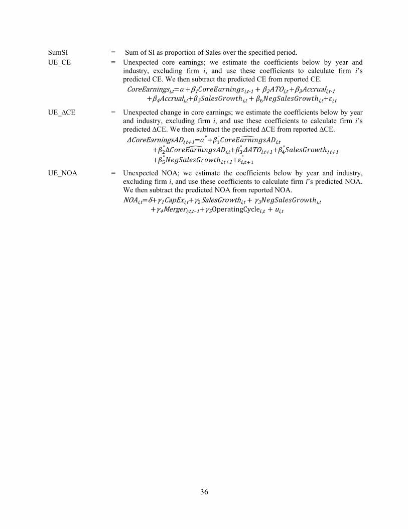
36

SumSI = Sum of SI as proportion of Sales over the specified period. UE_CE = Unexpected core earnings; we estimate the coefficients below by year and

industry, excluding firm i, and use these coefficients to calculate firm i’s predicted CE. We then subtract the predicted CE from reported CE.

CoreEarningsi,t α β1 i,t‐1 β2ATOi,t β3Accruali,t‐1 β4Accruali,t 5 i,t i,t i,t

UE_∆CE = Unexpected change in core earnings; we estimate the coefficients below by year and industry, excluding firm i, and use these coefficients to calculate firm i’s predicted ∆CE. We then subtract the predicted ∆CE from reported ∆CE.

∆CoreEarningsADi,t 1" "

i,t "∆ i,t

"∆ATOi,t 1"

i,t 1 "

i,t 1 ,"

UE_NOA = Unexpected NOA; we estimate the coefficients below by year and industry, excluding firm i, and use these coefficients to calculate firm i’s predicted NOA. We then subtract the predicted NOA from reported NOA.

NOAi,t δ γ1CapExi,t γ SalesGrowthi,t γ3 i,t γ4Mergeri;t,t–1 γ5OperatingCycle , ui,t

37

References

Anderson, M., R. Banker, and S. Janakiraman. 2003. Are Selling, General, and Administrative Costs ‘‘Sticky’’? Journal of Accounting Research 41: 47–63.

Angrist, J., and J. Pischke. 2009. Mostly Harmless Econometrics: An Empiricist’s Companion. Princeton University Press.

Atiase, R., D. Platt, and S. Tse. 2004. Operational Restructuring Charges and Post-Restructuring Performance. Contemporary Accounting Research 21 (3): 493–522.

Barton, J., and P. Simko. 2002. The Balance Sheet as an Earnings Management Constraint. The Accounting Review 77: 1–27.

Bens, D. and R. Johnston. 2009. Accounting Discretion: Use or Abuse? An Analysis of Restructuring Charges Surrounding Regulator Action. Contemporary Accounting Research 26: 673–699.

Bentley, J. T., Christensen, K. Gee, and B. Whipple. 2018. Disentangling managers’ and analysts’ non-GAAP reporting. Journal of Accounting Research 56 (4): 1039–1081.

Black, D. and T. Christensen. 2009. US Managers’ Use of ‘Pro Forma’ Adjustments to Meet Strategic Earnings Targets. Journal of Business Finance & Accounting 36: 297-326.

Bradshaw, M. and R. Sloan. 2002. GAAP versus the Street: An Empirical Assessment of Two Alternative Definitions of Earnings. Journal of Accounting Research 40: 41–66.

Brown, N., T. Christensen, W. Elliott, and R. Mergenthaler. 2012. Investor sentiment and pro forma earnings disclosures. Journal of Accounting Research 50: 1–40.

Burgstahler, D., J. Jiambalvo, and T. Shevlin. 2002. Do Stock Prices Fully Reflect the Implications of Special Items for Future Earnings? Journal of Accounting Research 40: 585–612.

Carhart, M. 1997. On Persistence in Mutual Fund Performance. Journal of Finance 52: 57-82. Choy, L. 2003. Impact of Earnings Management Flexibility. Working paper, University of

Rochester. Collins, D., E. Maydew, and I. Weiss. 1997. Changes in the Value-Relevance of Earnings and

Book Values over the Past Forty Years. Journal of Accounting and Economics 24: 39–67. Cready, W., T. Lopez and C. Sisneros. 2010. The Persistence and Market Valuation of Recurring

Nonrecurring Items. The Accounting Review 85: 1577–1615. DeAngelo, H., L. DeAngelo, and D. Skinner. 1994. Accounting Choice in Troubled Companies.

Journal of Accounting and Economics 17: 113–143. Dechow, P. and I. Dichev. 2002. The Quality of Accruals and Earnings: The Role of Accrual

Estimation Errors. The Accounting Review Supplement 77: 35-59. Dechow, P. and W. Ge. 2006. The Persistence of Earnings and Cash Flows and the Role of

Special Items: Implications for the Accrual Anomaly. Review of Accounting Studies 11: 253–296.

Dechow, P., M. Huson, and R. Sloan. 1994. The Effect of Restructuring Charges on Executives’ Cash Compensation. The Accounting Review 69: 138–156.

DeFond, M. 2002. Discussion of the Balance Sheet as an Earnings Management Constraint. The Accounting Review 77: 29–33.

Donelson, D., R. Jennings, and J. McInnis. 2011. Changes over Time in the Revenue-Expense Relation: Accounting or Economics? The Accounting Review 86: 945–974.

Doyle, J., R. Lundholm, and M. Soliman. 2003. The Predictive Value of Expenses Excluded from Pro Forma Earnings. Review of Accounting Studies 8: 145–174.

38

Doyle, J., J. Jennings, and M. Soliman. 2013. Do Managers Define Non-GAAP Earnings to Meet or Beat Analyst Forecasts? Journal of Accounting and Economics 56: 40–56.

Elliott, J., and J. Hanna. 1996. Repeated Accounting Write-Offs and the Information Content of Earnings. Journal of Accounting Research 34: 135–155.

Elliott, J., and W. Shaw. 1988. Write-Offs as Accounting Procedures to Manage Perceptions. Journal of Accounting Research 26 (Supplement): 91–119.

Fairfield, P., K. Kitching, and V. Tang. 2009. Are Special Items Informative about Future Profit Margins? Review of Accounting Studies, 14: 204–236.

Fairfield, P., R. Sweeney, and T. Yohn. 1996. Accounting Classification and the Predictive Content of Earnings. The Accounting Review 71: 337–355.

Fama, E., and K. French. 1992. The Cross-Section of Expected Stock Returns. Journal of Finance XLVII (2): 427–465.

Fama, E., and K. French. 1997. Industry Costs of Equity. Journal of Financial Economics 43 (2): 153–193.

Fan, Y., A. Barua, W. Cready, and W. Thomas. 2010. Managing Earnings Using Classification Shifting: Evidence from Quarterly Special Items. The Accounting Review 85: 1303–1323.

Francis, J., D. Hanna, and L. Vincent. 1996. Causes and Effects of Discretionary Asset Write-Offs. Journal of Accounting Research 34: 117–134.

Freeman, R., J. Ohlson and S. Penman. 1982. Book Rate-of-Return and Prediction of Earnings Changes: An Empirical Investigation. Journal of Accounting Research 20: 639–653.

Gaver, J., and K. Gaver. 1998. The Relation Between Nonrecurring Accounting Transactions and CEO Cash Compensation. The Accounting Review 73: 235–253.

Healy, P. 1985. The Effect of Bonus Schemes on Accounting Decisions. Journal of Accounting and Economics 7: 85–107.

Hirshleifer, D., K. Hou, S. H. Teoh, and Y. Zhang. 2004. Do Investors Overvalue Firms with Bloated Balance Sheets? Journal of Accounting and Economics 38: 297–331

Kinney, M., and R. Trezevant. 1997. The Use of Special Items to Manage Earnings and Perceptions. The Journal of Financial Statement Analysis Fall: 45–53.

Kirschenheiter, M., and N. Melumad. 2002. Can “Big Bath” and Earnings Smoothing Co-Exist as Equilibrium Financial Reporting Strategies? Journal of Accounting Research 40: 761–795.

Kolev, K., C. Marquardt, and S. McVay. 2008. SEC Scrutiny and the Evolution of Non-GAAP Reporting. The Accounting Review 83: 157–184

Lee, Y. 2014. An examination of restructuring charges surrounding the implementation of SFAS 146. Review of Accounting Studies 19: 539–572.

Levitt, A. 1998. The Numbers Game. Available at: http://www.sec.gov/news/speeches/spch220.txt.

Lipe, R. 1986. The Information Contained in the Components of Earnings. Journal of Accounting Research 24: 37–64.

Lougee B. and C. Marquardt. 2004. Earnings Informativeness and Strategic Disclosure: An Empirical Examination of “Pro Forma” Earnings. The Accounting Review 79: 769-795.

McVay, S. 2006. Earnings Management Using Classification Shifting: An Examination of Core Earnings and Special Items. The Accounting Review 81: 501–531.

Michaels, D. and M. Rapoport. 2016. SEC Signals It Could Curb Use of Adjusted Earnings Figures. Available at: http://www.wsj.com/articles/sec-scrutinizing-use-of-non-gaap-measures-by-public-companies-1458139473?mod=djemCFO_h.

39

Moehrle, S. 2002. Do Firms Use Restructuring Charge Reversals to Meet Earnings Targets? The Accounting Review 77: 397–413.

Moore, M. 1973. Management Changes and Discretionary Accounting Decisions. Journal of Accounting Research 11: 100–107.

Murphy, K. and J. Zimmerman. 1993. Financial Performance Surrounding CEO Turnover. Journal of Accounting and Economics 16: 273–315.

Nelson, M., J. Elliott, and R. Tarpley. 2002. Evidence from auditors about managers’ and auditors’ earnings management decisions. The Accounting Review 77 (Supplement): 175–202.

Nissim, D. and S. Penman. 2001. Ratio Analysis and Equity Valuation: From Research to Practice. Review of Accounting Studies 6: 109–154.

Ohlson, J. 1999. On Transitory Earnings. Review of Accounting Studies 4: 145–162. Philbrick, D., and W. Ricks. 1991. Using Value Line and I/B/E/S Analyst Forecasts in

Accounting Research. Journal of Accounting Research 29: 397–417. Pourciau, S. 1993. Earnings Management and Nonroutine Executive Changes. Journal of

Accounting and Economics 16: 317–336. Riedl, E. 2004. An Examination of Long-Lived Asset Impairments. The Accounting Review 79:

823–852. Riedl, E., and S. Srinivasan. 2010. Signaling Firm Performance through Financial Statement

Presentation: An Analysis Using Special Items. Contemporary Accounting Research 27: 289–332.

Robinson, L. 2010. Do Firms Incur Costs to Avoid Reducing Pre-Tax Earnings? Evidence from the Accounting for Low-Income Housing Tax Credits. The Accounting Review 85: 637–669.

Skaife, H., and D. Wangerin. 2013. Target financial reporting quality and M&A deals that go bust. Contemporary Accounting Research 30 (2): 719–749.

Sloan, R. 1996. Do Stock Prices Fully Reflect the Information in Accruals and Cash Flows about Future Earnings? The Accounting Review 71: 289–315.

40

Figure 1: Incidence and Intensity of Income-decreasing Special Items through Time

The graph reflects the frequency (solid line; left axis) and intensity (dashed line; right axis), as percentage of net sales, income-decreasing special items by fiscal year among firms with positive total assets and sales, as reported by Compustat. Intensity is winsorized at 99% by fiscal year. Figure 2: OppSI Intensity

The graph presents the time-series of the ratio of estimated opportunistic to total special items. The dashed line corresponds to the main model used in the paper, where the proportion of opportunistic special items is based on the model residual, and the solid line reflects the fitted value model estimates, referenced in Section 4.3.

0

0.02

0.04

0.06

0.08

0.1

0.12

0.14

0.16

0.18

0.2

0.05

0.1

0.15

0.2

0.25

0.3

0.35

0.4

0.45

0.5

0.551980

1981

1982

1983

1984

1985

1986

1987

1988

1989

1990

1991

1992

1993

1994

1995

1996

1997

1998

1999

2000

2001

2002

2003

2004

2005

2006

2007

2008

2009

2010

2011

2012

2013

2014

2015

2016

Frequency Intensity

0.2

0.3

0.4

0.5

0.6

0.7

0.8

0.9

1989

1990

1991

1992

1993

1994

1995

1996

1997

1998

1999

2000

2001

2002

2003

2004

2005

2006

2007

2008

2009

2010

2011

2012

2013

2014

2015

2016

%LQSI; Fitted Value Model %LQSI; Residual Value Model

41

Table 1

Panel A: Descriptive Statistics, Pooled Sample # Obs. Mean Q1 Median Q3 StdDev Total Assetst 104,495 6,757.96 67.66 403.91 2,192.44 32,022.35 Net Salest 104,495 2,908.08 51.45 259.87 1,318.69 9,600.77 Pre-tax Incomet / Net Salest 104,495 –0.0301 –0.0227 0.0540 0.1347 0.4992 Core Earningst / Net Salest 101,350 0.0861 0.0426 0.1168 0.2301 0.4128 Special Itemst / Net Salest 104,495 0.0244 0.0000 0.0000 0.0102 0.0842 Sales Growtht 104,495 0.0925 –0.0420 0.0599 0.1789 0.2955 Losst 104,495 0.2537 0.0000 0.0000 1.0000 0.4351 ATOt 100,083 2.5032 0.7598 1.6233 2.8436 3.4591 BMt 104,078 0.5808 0.2976 0.5453 0.8922 1.6474 OppSIt 104,495 0.0163 0.0000 0.0000 0.0043 0.0580 PredSIt 104,495 0.0107 0.0000 0.0000 0.0000 0.0391 OppSI 90,972 0.0084 0.0000 0.0000 0.0000 0.0322 PredSI 90,972 0.0187 0.0000 0.0000 0.0035 0.0716 NIBTSIt / Net Salest 104,495 –0.0003 –0.0018 0.0622 0.1429 0.4443 ∑ NIBTSI /NetSales 83,275 0.0416 0.0046 0.1188 0.2670 0.6725 CFOt / Net Salest 104,495 0.0696 0.0210 0.0876 0.1879 0.3541 ∑ CFO /NetSales 83,141 0.1626 0.0517 0.1678 0.3500 0.5502 ∑ BHAR 67,581 0.0805 –0.3941 –0.0352 0.3296 0.8489

Panel B: Descriptive Statistics, Observations with Income-Decreasing Special Items versus No Income-Decreasing Special Items Income-Decreasing

Special Items No Income-Decreasing

Special Items Equality of

Means / Medians Variables # Obs. Mean Median # Obs. Mean Median

Total Assetst 42,788 8,828.02 682.60 61,707 5,322.57 208.15 0.01 / 0.01 Net Salest 42,788 3,857.55 465.95 61,707 2,249.71 167.37 0.01 / 0.01 Pre-tax Incomet/Net Salest 42,788 –0.0983 0.0255 61,707 0.0171 0.0719 0.01 / 0.01 Core Earningst/Net Salest 41,772 0.0713 0.1109 59,578 0.0966 0.1208 0.01 / 0.01 Special Itemst/Net Salest 42,788 0.0596 0.0163 61,707 0.0000 0.0000 0.01 / 0.01 Sales Growtht 42,788 0.0770 0.0442 61,707 0.1032 0.0707 0.01 / 0.01 Losst 42,788 0.3086 0.0000 61,707 0.2156 0.0000 0.01 / 0.01 ATOt 41,140 2.4643 1.5708 58,943 2.5304 1.6651 0.01 / 0.01 BMt 42,634 0.5025 0.5218 61,444 0.6350 0.5606 0.01 / 0.01 OppSIt 42,788 0.0397 0.0087 61,707 0.0000 0.0000 0.01 / 0.01 PredSIt 42,788 0.0262 0.0000 61,707 0.0000 0.0000 0.01 / 0.01 OppSI 36,228 0.0210 0.0015 54,744 0.0000 0.0000 0.01 / 0.01 PredSI 36,228 0.0471 0.0089 54,744 0.0000 0.0000 0.01 / 0.01 NIBTSIt / Net Salest 42,788 –0.0302 0.0480 61,707 0.0204 0.0719 0.01 / 0.01 ∑ NIBTSI /NetSales 32,625 0.0242 0.1086 50,650 0.0528 0.1258 0.01 / 0.01 CFOt / Net Salest 42,788 0.0572 0.0829 61,707 0.0781 0.0910 0.01 / 0.01 ∑ CFO /NetSales 32,588 0.1491 0.1642 50,553 0.1714 0.1705 0.01 / 0.01 ∑ BHAR 27,275 0.0934 –0.0237 40,306 0.0717 –0.0441 0.01 / 0.01

All variables are as defined in Appendix 2. All continuous variables are winsorized at 1% and 99% by fiscal year. The last column reports the p-values for a t-test for equality of means and median test for equality of medians.

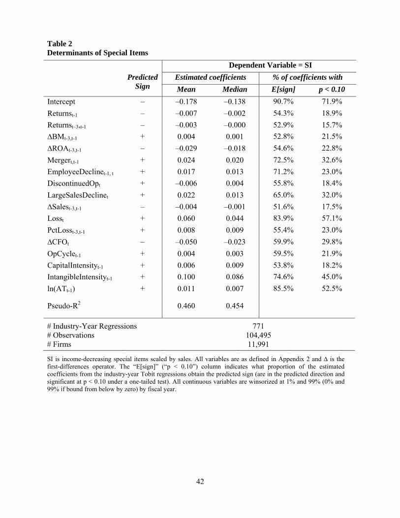
42

Table 2 Determinants of Special Items

Dependent Variable = SI

Predicted Sign

Estimated coefficients % of coefficients with

Mean Median E[sign] p < 0.10

Intercept – –0.178 –0.138 90.7% 71.9%

Returnst-1 – –0.007 –0.002 54.3% 18.9%

Returnst–3,t-1 – –0.003 –0.000 52.9% 15.7%

∆BMt-3,t-1 + 0.004 0.001 52.8% 21.5%

∆ROAt-3,t-1 – –0.029 –0.018 54.6% 22.8%

Mergert,t-1 + 0.024 0.020 72.5% 32.6%

EmployeeDeclinet-1, t + 0.017 0.013 71.2% 23.0%

DiscontinuedOpt + –0.006 0.004 55.8% 18.4%

LargeSalesDeclinet + 0.022 0.013 65.0% 32.0%

∆Salest-3,t-1 – –0.004 –0.001 51.6% 17.5%

Losst + 0.060 0.044 83.9% 57.1%

PctLosst-3,t-1 + 0.008 0.009 55.4% 23.0%

∆CFOt – –0.050 –0.023 59.9% 29.8%

OpCyclet-1 + 0.004 0.003 59.5% 21.9%

CapitalIntensityt-1 + 0.006 0.009 53.8% 18.2%

IntangibleIntensityt-1 + 0.100 0.086 74.6% 45.0%

ln(ATt-1) + 0.011 0.007 85.5% 52.5%

Pseudo-R2 0.460 0.454

# Industry-Year Regressions 771 # Observations 104,495 # Firms 11,991

SI is income-decreasing special items scaled by sales. All variables are as defined in Appendix 2 and ∆ is the first-differences operator. The “E[sign]” (“p < 0.10”) column indicates what proportion of the estimated coefficients from the industry-year Tobit regressions obtain the predicted sign (are in the predicted direction and significant at p < 0.10 under a one-tailed test). All continuous variables are winsorized at 1% and 99% (0% and 99% if bound from below by zero) by fiscal year.

43

Table 3 Regressing Future Pre-Tax, Pre-SI Income on Predicted and Opportunistic Special Items

Predicted Sign

Dependent Variable = ∑

Full Sample SI Sample OppSI Sample

SIt ? 0.007 –0.125 –0.132 (0.12) (–1.98) (–2.02)

PredSIt ? 0.388 0.222 0.415 (3.85) (2.06) (2.30)

OppSIt – –0.137 –0.266 –0.356 (–1.70) (–3.22) (–3.66)

NIBTSIt + 1.036 1.038 1.024 1.028 1.012 1.016 (46.49) (46.66) (31.08) (31.22) (28.12) (28.29)

Sales Growtht ? –0.078 –0.076 –0.091 –0.087 –0.107 –0.103 (–6.30) (–6.09) (–5.00) (–4.80) (–5.25) (–5.05)

Ind-Year Fixed Effects Included Included Included Included Included Included

# Observations

83,275 83,275 32,625 32,625 25,972 25,972

# Firms 9,664 9,664 7,621 7,621 7,300 7,300

Adj. R2 0.412 0.412 0.413 0.413 0.416 0.417

PredSIt = OppSIt

0.001 0.001 0.001

The dependent variable is Net Income before Taxes and Special Items scaled by contemporaneous Sales cumulated over years t+2 through t+3. All variables are as defined in Appendix 2. All continuous variables are winsorized at 1% and 99% (0% and 99% if bound from below by zero) by fiscal year. The full sample comprises all observations with sufficient data to estimate OppSI; the SI (OppSI) sample further requires the recognition of income-decreasing special items (identification of OppSI) in year t. All models are estimated using OLS and include industry-year fixed effects. The standard errors are clustered by firm. We report the t-statistics in brackets below the estimated coefficients. The main variable(s) of interest are in bold.

44

Table 4 Regressing Future Cash Flows on Predicted and Opportunistic Special Items

Predicted Sign



SIt ? –0.056 –0.120 –0.126 (–1.27) (–2.61) (–2.61)

PredSIt ? 0.207 0.115 0.147 (2.62) (1.35) (1.07)

OppSIt – –0.163 –0.222 –0.250 (–2.74) (–3.65) (–3.39)

CFOt + 1.048 1.049 1.057 1.059 1.037 1.039 (47.59) (47.74) (36.43) (36.61) (33.19) (33.31)

Sales Growtht

? –0.022 –0.021 –0.022 –0.019 –0.026 –0.024 (–2.23) (–2.07) (–1.53) (–1.35) (–1.63) (–1.52)

AccrualsPre-SIt + 0.345 0.346 0.360 0.363 0.369 0.371

(14.84) (14.90) (10.29) (10.34) (10.05) (10.12)


# Observations

83,141 83,141 32,588 32,588 25,943 25,943

# Firms 9,650 9,650 7,615 7,615 7,294 7,294

Adj. R2 0.458 0.458 0.463 0.463 0.467 0.467

PredSIt = OppSIt

0.001 0.002 0.030

The dependent variable is CFO scaled by contemporaneous Sales cumulated over years t+2 through t+3. All variables are as defined in Appendix 2. All continuous variables are winsorized at 1% and 99% (0% and 99% if bound from below by zero) by fiscal year. The full sample comprises all observations with sufficient data to estimate OppSI; the SI (OppSI) Sample further requires the recognition of income-decreasing special items (identification of OppSI) in year t. All models are estimated using OLS and include industry-year fixed effects. The standard errors are clustered by firm. We report the t-statistics in brackets below the estimated coefficients. The p-value of the test on coefficient equivalence, PredSIt = OppSIt, is two-tailed. The main variable(s) of interest are in bold.

45

Table 5 Regressing Future Returns on Predicted and Opportunistic Special Items

Predicted Sign



SIt ? –0.212 –0.271 –0.254 (–4.02) (–4.78) (–4.39)

PredSIt ? –0.091 –0.167 –0.258 (–0.72) (–1.24) (–1.31)

OppSIt – –0.240 –0.306 –0.268 (–2.98) (–3.63) (–2.74)

Betat + 0.009 0.008 0.002 0.001 –0.004 –0.004 (1.34) (1.28) (0.22) (0.16) (–0.43) (–0.43)

Momentumt – –0.081 –0.080 –0.099 –0.099 –0.105 –0.105 (–6.76) (–6.73) (–5.68) (–5.65) (–5.22) (–5.22)

AccrualsPre-SIt –

0.038 0.039 0.041 0.043 0.045 0.044 (1.69) (1.73) (1.21) (1.24) (1.20) (1.19)

BMt + 0.024 0.025 0.020 0.020 0.017 0.017 (3.70) (3.70) (2.87) (2.88) (2.39) (2.37)

ln(MVEt) – –0.009 –0.009 –0.013 –0.012 –0.012 –0.012 (–3.96) (–3.90) (–4.09) (–3.98) (–3.36) (–3.35)


# Observations

45,593 45,593 21,023 21,023 16,327 16,327

# Firms 6,175 6,175 4,908 4,908 4,681 4,681

Adj. R2 0.115 0.115 0.127 0.126 0.123 0.122

PredSIt = OppSIt

0.390 0.441 0.970

The dependent variable is market-adjusted buy-and-hold returns cumulated over years t+2 through t+3 starting the month after the earnings announcement for year T. All variables are as defined in Appendix 2. All continuous independent variables are winsorized at 1% and 99% (0% and 99% if bound from below by zero) by fiscal year. The full sample comprises all observations with sufficient data to estimate OppSI; the SI (OppSI) Sample further requires the recognition of income-decreasing special items (identification of OppSI) in year t. All models are estimated using OLS and include industry-year fixed effects. The standard errors are clustered by firm. We report the t-statistics in brackets below the estimated coefficients. The p-value of the test on coefficient equivalence, PredSIt = OppSIt, is two-tailed. The main variable(s) of interest are in bold.

46

Table 6 Panel A: Future Accounting Restatements on Special Items

Predicted Sign Dependent Variable = Restate

SIt ? 0.024 0.026 (2.68) (2.72)

PredSIt ? 0.005 0.006 (0.16) (0.20)

OppSIt + 0.035 0.038 (2.39) (2.42)

Controls Not Included Not Included Included Included Industry-Year Fixed Effects Included Included Included Included

# Observations 25,379 25,379 25,199 25,199 # Firms 7,256 7,256 7,226 7,226 Adj. R2 0.012 0.012 0.013 0.013 PredSIt = OppSIt 0.457 0.436

This panel provides the estimation of Equation (3) in Section 4.2.2.1. Restate is an indicator variable set to one if the fiscal year overlaps with a restatement period for the company and the restatement is 1) classified as related to accounting issues or fraud, and 2) the description of the restatement contains at least one of the key words related to SI. All other variables are as defined in Appendix 2. All continuous variables are winsorized at 1% and 99% (0% and 99% if bound from below by zero) by fiscal year. The sample comprises observations with OppSI > 0 in year t. All models are estimated using a linear probability model and include industry-year fixed effects. The standard errors are clustered by firm. We report the t-statistics in brackets below the estimated coefficients. The p-value of the test on coefficient equivalence, PredSIt = OppSIt, is two-tailed. The main variable(s) of interest are in bold. Panel B: Regression of Analyst Benchmark Outcomes on %OppSI Dependent Variable = Predicted Sign %MBEt %MBEt-1 %MBEt+1 SI

Sample OppSI Sample

SI Sample

OppSI Sample

SI Sample

OppSI Sample

%OppSIt + 0.026 0.056 0.015 0.031 0.012 0.022 (4.88) (5.53) (2.79) (3.06) (2.08) (1.98)

Controls Included Included Included Included Included Included Industry-Year Fixed Effects Included Included Included Included Included Included # Observations 27,606 21,618 26,616 20,776 24,686 19,378 # Firms 5,966 5,655 5,753 5,430 5,404 5,131 Adj. R2 0.099 0.108 0.111 0.119 0.099 0.105

This panel provides the estimation of Equation (4) in Section 4.2.2.2. Regressions are estimated using a linear probability model. %MBEt is the ratio of the quarters in the one year window of fiscal year t where the median consensus analyst forecast error is between zero and two cents per share. All other variables are as defined in Appendix 2. t-statistics are reported in brackets below the estimated coefficients. The errors are clustered by firm. The variable of interest is in bold. The SI Sample comprises firm-year observations with income-decreasing special items and sufficient data to estimate the proportion of opportunistic special items; the OppSI sample further requires the identification of OppSI during the period. The continuous variables, other than %MBE and %OppSI, are winsorized at 1% and 99% by fiscal year. The main variable of interest is in bold.

47

Table 7 Regression of OppSI on proxies for shifting from the past, present, and future

Predicted Sign

Dependent Variable = OppSI Tobit OLS Full

Sample SI

Sample OppSI Sample

Full Sample

SI Sample

OppSI Sample

UE_NOAt-1 + 0.004 0.007 0.009 0.003 0.007 0.009 (6.26) (7.84) (9.53) (8.23) (8.54) (9.38)

UE_CEt + 0.064 0.065 0.070 0.033 0.059 0.070 (10.34) (8.42) (8.53) (9.65) (8.44) (8.39)

UE_∆CEt+1 + 0.017 –0.002 0.008 0.006 0.002 0.008 (3.48) (–0.34) (1.23) (2.36) (0.34) (1.21)

UE_∆CEt+2 + 0.013 0.000 0.006 0.004 0.003 0.006 (2.96) (0.09) (1.07) (2.02) (0.56) (1.06)

Industry-Year Fixed Effects

Included Included Included Included Included Included

# Observations 74,505 29,442 23,303 74,505 29,442 23,303 # Firms 8,964 7,031 6,711 8,964 7,031 6,711

Pseudo-R2 0.439 –0.084 –0.077 Adj. R2 0.047 0.093 0.127

OppSI is the estimate of opportunistic special items measured as the residual from Equation (1). The full sample comprises firm-year observations with sufficient data to measure OppSI; the SI > 0 subsample further requires the reporting of an income-decreasing special item during the period. The standard errors are clustered by firm. We report the t-statistics in brackets below the estimated coefficients. Variable(s) of interest are in bold. All variables are as defined in Appendix 2. All continuous variables are winsorized at 1% and 99% (0% and 99% if bound from below by zero) by fiscal year.

48

Online Appendix to “Detecting Opportunistic Special Items”

Online Appendix A

A.1 Abnormal Past Performance (UE_NOA)

We estimate abnormal past performance via the model described by Equation (A.1). We use Net

Operating Assets (NOA), which has been linked to balance sheet bloat (Barton and Simko 2002;

Hirshleifer et al. 2004), as a proxy for the accumulation of assets (e.g., accounts receivable, inventory,

equipment) that should have been expensed in the normal course of business. For example, a manager

might recognize too little bad debt expense, or might depreciate equipment too slowly, both of which

will result in the accumulation of past expenses as assets (e.g., net A/R or net PP&E) on the balance

sheet. An alternative approach would entail examining unexpected earnings performance over a discrete

set of prior years, analogous to our measure of shifting from the future we discuss below. Such a design,

however, would only capture shifting over a limited period, whereas asset bloat allows for assessing the

cumulative effect.

Ideally, we would isolate asset accumulation related to the intentional under-expensing of past

assets; however, some asset accumulation may be due to errors in the estimation of needed inventory or

industry downturns. Moreover, both DeFond (2002) and Choy (2003) note that industry is a necessary

control when assessing net operating assets. Thus, to lower the likelihood that industry-wide and

macroeconomic shocks are bundled into the error term, we estimate Equation (A.1) below within

industry and year. The abnormal NOA model we consider takes the form:

NOAi,t δ γ1CapExi,t γ SalesGrowthi,t γ3 i,t γ4Mergeri;t,t–1 γ5OperatingCycle , ui,t

(A.1)

Following prior research (e.g., Hirshleifer et al. 2004), we measure NOA as the difference

between Operating Assets and Operating Liabilities. We scale NOA by Sales, to be consistent with the

scaling of special items. As predictors, we consider Sales Growth and Capital Expenditures, since the

accumulation of assets could be due to a decrease in product demand or in anticipation of an expansion

49

in operations. We allow for a separate slope for decline in sales to account for asymmetric ratcheting

(Anderson et al. 2003). We also include an indicator variable for merger or acquisition activity in years t

or t–1, as we expect M&A to result in shocks to NOA. Finally, we include the length of the firm’s

operating cycle, as it directly relates to asset build-up. To avoid bias from the reporting choices of each

examined firm, we estimate the necessary industry-year coefficients excluding firm i.

We apply the estimated coefficients to calculate firm i’s predicted NOA. We retain the

regression residual as a measure of UE_NOA. We present the mean and median coefficient in Table

A.1, Panel A; the mean R2 is 30.4 percent.18

As initial support for the claim that our measure of past abnormal performance is in part a

function of intentional accumulation of past expenses, we document a significantly negative correlation

between abnormal net operating assets and industry-year-median adjusted allowance for bad debts and

depreciation rates (Table A.2). In particular, abnormal net operating assets are higher when the firm’s

percentage of allowance for doubtful accounts is below the industry median and when the firm’s

depreciation rate is below the industry median. Although by itself the estimate could capture assets that

are more productive, coupled with the subsequent reporting of an income-decreasing special item, the

observed effect points to a systematic under-estimation of recurring expenses. The associations are

persistent year-over-year, consistent with the stickiness of both depreciation rates and allowance for

doubtful accounts estimates. In other words, if the abnormal net operating assets were a result of good

performance, or unanticipated shocks to the firm or industry, we would not expect to find a

systematically negative relation with these previously recorded subjective accounting estimates.

Turning to assessing the quality of special items, if managers delay normal operating expenses

and later write them off as special items, the subsequently reported special items should increase in

18 We do not include the level of NOA in the prior period as an explanatory variable as this specification would model the unexpected change in NOA, rather than the level of NOA. As a practical matter, if we include NOAt-1 as an explanatory variable in model (A.1), the average (median) R2 jumps to 75.8 percent (80.2 percent). Although modeling the change in NOA weakens the observed effects, the main inferences we report are unaffected (not tabulated).

50

abnormal net operating assets. Thus, we expect unexpected net operating assets at the end of year t–1 to

be positively associated with income-decreasing special items in year t. Consistent with this conjecture,

we document a positive correlation between income-decreasing special items (SIt / Net Salest) and

unexpected net operating assets (UE_NOAt-1; untabulated).

A portion of the estimated abnormal net operating assets likely reflects superior past

performance. This component, however, should not be associated with subsequent income-decreasing

special items. In other words, the refinement to the methodology to estimate opportunistic special items

we propose attributes only the component of abnormal net operating assets associated with special

items, not the entire value of UE_NOA, to the accumulation of past expenses.

A.2 Abnormal Current Performance (UE_CE)

Next, we turn to abnormal current performance. We base our model of abnormal core earnings

on McVay (2006), as follows:

CoreEarningsi,t α β1 i,t‐1 β2ATOi,t β3Accruali,t‐1 β4Accruali,t 5 i,t i,t i,t

(A.2)

where we define Core Earnings as Operating Income before Depreciation and Amortization for the year,

as reported by Compustat (Compustat item OIBDP), scaled by Net Sales for the year. Like McVay

(2006), we focus on earnings before depreciation and amortization to avoid mechanical reductions in

current period depreciation and amortization expense resulting from current-period asset write-downs.

The vector of controls includes the prior period level of core earnings in Equation (A.2) as core earnings

should persist. We also consider the asset turnover ratio (ATO), as special items may be associated with

firm strategy, and core earnings (which, when scaled by Sales, approximate a firm’s profit margin) is

expected to shift with asset turnover (Nissim and Penman 2001). We include both prior period and

current period accruals; holding earnings constant, accruals yield less persistent earnings than cash flows

(Sloan 1996). Current period accruals are included by McVay (2006) as a performance control, as

extreme performance is highly correlated with changes in accrual levels (DeAngelo et al. 1994). Mindful

51

of potential endogeneity, we also consider an alternate model of current period shifting proposed by Fan

et al. (2010), which excludes this variable, as a robustness check; inferences are not affected

(untabulated). Finally, we include sales growth—as sales increase, fixed costs per sales dollar are

expected to be lower—and allow the coefficient to vary for sales declines, as Anderson et al. (2003) find

that costs are more sensitive to activity increases than to equivalent decreases.

We estimate the Equation (A.2) coefficients by year and industry, excluding firm i. Similar to the

NOA approach, estimating the model by industry-year allows the coefficients on each of the variables to

vary by industry-year and pushes industry and macro-economic shocks to the predicted value. We

measure unexpected core earnings (UE_CE) as the difference between the reported and predicted values

of Core Earnings.

We present the mean and median estimates from the industry-year regressions in Table A.1,

Panel B. The mean R2 of the model is 79.2 percent and the coefficients are generally in the predicted

direction and are comparable to those reported in McVay (2006). Our arguments indicate unexpected

current core earnings to increase in income-decreasing special items.19 In other words, as core expenses

are misclassified as special items, we expect unexpected core earnings to become more positive.

A.3 Abnormal Future Performance (UE_∆CE)

We operationalize abnormal future performance through the unexpected improvements in

earnings over the two years after reporting of the respective income-decreasing special item. We

acknowledge that benefits gained by accelerating depreciation or other recurring expenses to the current

period special item often extend beyond the next two years. We opt for a two-year window as a

compromise between capturing the full economic effect of shifting future recurring expenses and the

19 If managers shift core expenses to special items every period, our expectations models would be based on artificially inflated core earnings figures, thereby weakening the power of our tests. Investors, however, should begin to weight repeat special items more in line with recurring earnings (Elliott and Hanna 1996; Cready et al. 2010). Thus, managers are precluded from using special items to manage earnings every period if they desire the lower weighting on these charges.

52

associated data costs and measurement challenges associated with considering a longer horizon.20

Hence, our future abnormal performance measure captures a lower bound of the effects of shifting from

the future.21 As a proxy for abnormal performance resulting from shifting of recurring expenses from the

future, we consider the residual from the following model:

∆CoreEarningsADi,t 1" "

i,t"∆ i,t

"∆ATOi,t 1"

i,t 1"

i,t 1 ,"

(A.3)

This model is an adaptation of Equation (A.2). We apply four adjustments. First, we consider

future core earnings after depreciation and amortization (Compustat item OIADP) to allow for the

acceleration of future depreciation and amortization via the write-off of a productive asset. Second, we

consider a changes, rather than levels, analysis. We take this approach with the aim of capturing the

annual increment of overstated earnings. To adapt the model to changes, we include both the level and

the change in core earnings, as mean reversion is expected to vary based on the level of earnings

(Freeman et al. 1982). We also consider the change, rather than the level, in asset turnover. Third, since

we require abnormal core earnings estimates based on pre-managed earnings, we consider the fitted

values of the level and change in core earnings, rather than the reported (and potentially managed)

values.22 Finally, we do not include accruals in the model, as inter-period shifting affects accruals.

20 Ideally, we would use a measure of cumulative shift of future expenses, analogous with the shifting of expenses from the past, UE_NOA, model. The described annual metric we use as a substitute poses a need to compromise between power of the tests on one hand, and sample attrition and survivorship bias, on the other. As a practical matter, we confirm that power of the test is a non-trivial issue with such a specification by annualizing the NOA measure (i.e., we model the change in NOA), noting that the results from shifting from the past only for years t-1 and t-2 notably weakens the inferences (not tabulated). 21 Ideally, as with the shifting of past expenses, we would like to consider a measure that reflects all future years of shifted expenses; for example, abnormal net operating assets at the end of year t. Theoretically, the abnormally low portion of net operating assets would reflect future expenses that were written off prematurely. It is possible, however, that net operating assets are abnormally low for performance-related reasons, and this abnormally low component of net operating assets would be correlated with special items, but not be reflective of opportunism. It is also possible that our measure of future write-offs could be capturing desirable levels of conservatism or performance improvements following a turn-around effort. These alternative explanations, however, would not predict an association with future restatements, or an association with lower future earnings and cash flows in year t+3. Moreover, these concerns extend only to shifting from the future, which comprises only 40 percent of our estimate of opportunistic special items for the mean company with positive OppSI (not tabulated). 22 We estimate the fitted values using a version of Equation (A.2), which focuses on the level and change in core earnings after, rather than before, depreciation and amortization. This ensures consistency between the left- and right-hand side variables.

53

As before, we form our estimate of the future change in core earnings by year and industry,

where the coefficients are estimated excluding firm i. Thus, we derive the unexpected change in future

earnings (UE_∆CE) as the reported value less the predicted value of the metric. We present the mean

and median results of the estimation for year t + 1 in Table A.1, Panel C. The mean and median R2 is

over 40 percent.

As with our other measures of abnormal performance, we conjecture the unexpected change in

future earnings would be positively associated with income-decreasing special items. Specifically, if

managers accelerate future core expenses into a current period special item, then, we expect income-

decreasing special items to increase in unexpected future earnings. Consistent with this notion, we note a

small, but statistically significant, positive correlation between special items and both UE_∆CEt+1 and

UE_∆CEt+2 (untabulated). An alternative interpretation of this correlation is that our estimate of shifting

from the future captures real economic improvements highlighting the need to examine future cash

flows and returns to present a more complete depiction of the underlying relations.

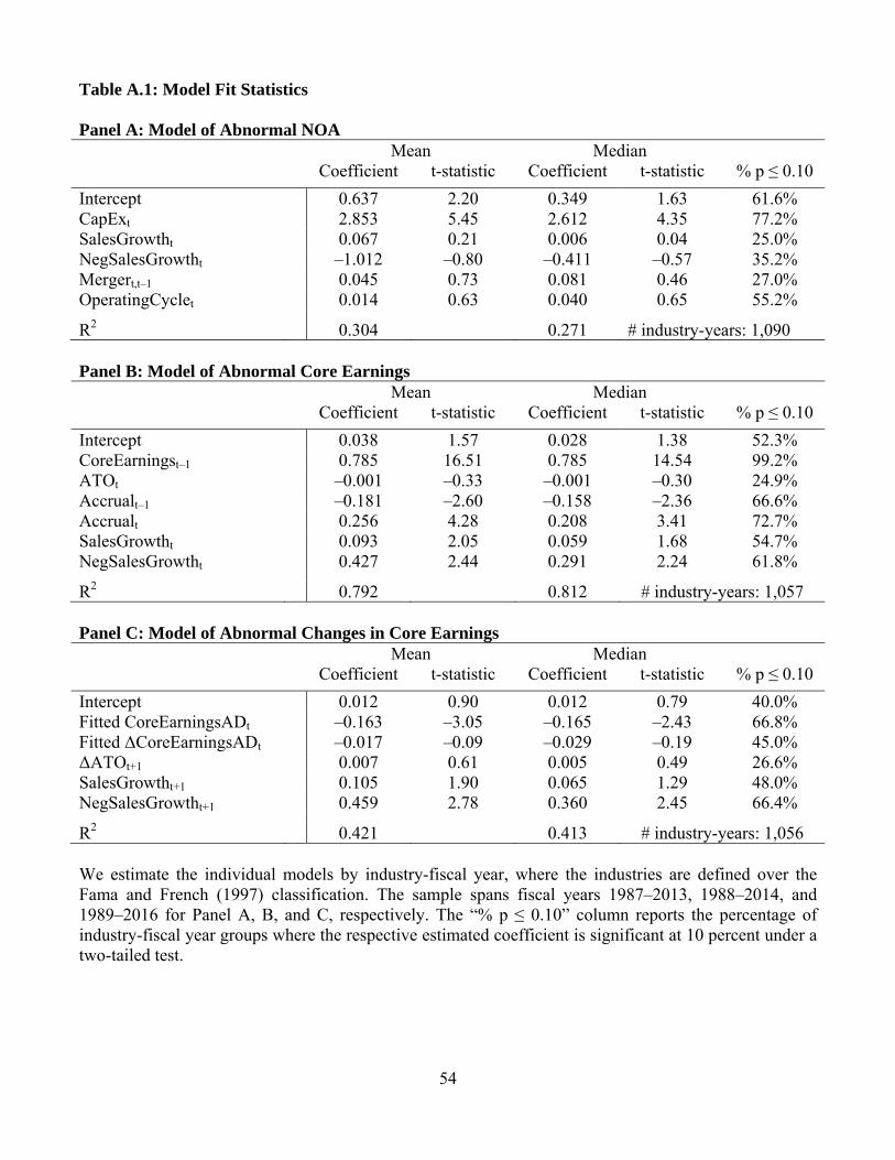
54

Table A.1: Model Fit Statistics Panel A: Model of Abnormal NOA Mean Median Coefficient t-statistic Coefficient t-statistic % p ≤ 0.10

Intercept 0.637 2.20 0.349 1.63 61.6% CapExt 2.853 5.45 2.612 4.35 77.2% SalesGrowtht 0.067 0.21 0.006 0.04 25.0% NegSalesGrowtht –1.012 –0.80 –0.411 –0.57 35.2% Mergert,t–1 0.045 0.73 0.081 0.46 27.0% OperatingCyclet 0.014 0.63 0.040 0.65 55.2%

R2 0.304 0.271 # industry-years: 1,090 Panel B: Model of Abnormal Core Earnings Mean Median Coefficient t-statistic Coefficient t-statistic % p ≤ 0.10

Intercept 0.038 1.57 0.028 1.38 52.3% CoreEarningst–1 0.785 16.51 0.785 14.54 99.2% ATOt –0.001 –0.33 –0.001 –0.30 24.9% Accrualt–1 –0.181 –2.60 –0.158 –2.36 66.6% Accrualt 0.256 4.28 0.208 3.41 72.7% SalesGrowtht 0.093 2.05 0.059 1.68 54.7% NegSalesGrowtht 0.427 2.44 0.291 2.24 61.8%

R2 0.792 0.812 # industry-years: 1,057 Panel C: Model of Abnormal Changes in Core Earnings Mean Median Coefficient t-statistic Coefficient t-statistic % p ≤ 0.10

Intercept 0.012 0.90 0.012 0.79 40.0% Fitted CoreEarningsADt –0.163 –3.05 –0.165 –2.43 66.8% Fitted ΔCoreEarningsADt –0.017 –0.09 –0.029 –0.19 45.0% ΔATOt+1 0.007 0.61 0.005 0.49 26.6% SalesGrowtht+1 0.105 1.90 0.065 1.29 48.0% NegSalesGrowtht+1 0.459 2.78 0.360 2.45 66.4%

R2 0.421 0.413 # industry-years: 1,056 We estimate the individual models by industry-fiscal year, where the industries are defined over the Fama and French (1997) classification. The sample spans fiscal years 1987–2013, 1988–2014, and 1989–2016 for Panel A, B, and C, respectively. The “% p ≤ 0.10” column reports the percentage of industry-fiscal year groups where the respective estimated coefficient is significant at 10 percent under a two-tailed test.

55

Table A.2 Correlation Matrix – Unexpected NOA and Intentional Expense Accumulation

(1) (2) (3) (4) (5) (6) (7)

(1) UE_NOAt - –0.0376 –0.1147 –0.2099 –0.0396 –0.1264 –0.2137 (0.001) (0.001) (0.001) (0.001) (0.001) (0.001)

(2) %DoubtfulAccounts_Adjt –0.0081 - 0.0414 0.0663 0.8285 0.0461 0.0588 (0.010) (0.001) (0.001) (0.001) (0.001) (0.001)

(3) DepreciationRate(Gross)_Adjt –0.0593 0.0420 - 0.6384 0.0302 0.8472 0.5265 (0.001) (0.001) (0.001) (0.001) (0.001) (0.001)

(4) DepreciationRate(Net)_Adjt –0.1063 0.0845 0.6736 - 0.0691 0.5892 0.8816 (0.001) (0.001) (0.001) (0.001) (0.001) (0.001)

(5) %DoubtfulAccounts_Adjt–1 –0.0073 0.7730 0.0281 0.0864 - 0.0438 0.0669 (0.021) (0.001) (0.001) (0.001) (0.001) (0.001)

(6) DepreciationRate(Gross)_Adjt–1 –0.0650 0.0502 0.7643 0.5557 0.0492 - 0.6586

(0.001) (0.001) (0.001) (0.001) (0.001) (0.001)

(7) DepreciationRate(Net)_Adjt–1 –0.1028 0.0711 0.4799 0.7968 0.0829 0.7064 - (0.001) (0.001) (0.001) (0.001) (0.001) (0.001)

Pearson (Spearman) correlations are below (above) the diagonal. UE_NOA is the residual from model 1. %DoubtfulAccounts is the ratio of Estimated Doubtful Receivables to Total Receivables plus Estimated Doubtful Receivables (Compustat items RECDt / (RECTt + RECDt)). DepreciationRate(Gross) is the ratio of depreciation expense to average gross PPE (Compustat items (DPt – AMt) / ((PPEGTt + PPEGTt-1)/2)). DepreciationRate(Net) is the ratio of depreciation expense to average gross PPE (Compustat items (DPt – AMt) / ((PPENTt + PPENTt-1)/2)). _Adj signifies that the variables are deviations from the industry-year median. p-values are reported in brackets below the correlation coefficients.

56

Table B Correlation Matrix – Main Variables

(1) (2) (3) (4) (5) (6) (7)

(1) PredSIt - 0.3375 –0.2536 –0.3138 –0.1528 –0.1547 –0.0158 (0.001) (0.001) (0.001) (0.001) (0.001) (0.001)

(2) OppSIt 0.4110 - –0.3025 –0.3710 –0.2306 –0.2090 –0.0197 (0.001) (0.001) (0.001) (0.001) (0.001) (0.001)

(3) CFOt –0.1629 –0.1922

(0.001) - 0.7658 0.5367 0.6505 0.0295

(0.001) (0.001) (0.001) (0.001) (0.001)

(4) NIBTSIt –0.2149 –0.2504 0.7412 - 0.6119 0.5842 0.0315 (0.001) (0.001) (0.001) (0.001) (0.001) (0.001)

(5) ∑ NIBTSI –0.0972 –0.1427 0.5310 0.6055 - 0.7515 0.1255 (0.001) (0.001) (0.001) (0.001) (0.001) (0.001)

(6) ∑ CFO –0.0959 –0.1270 0.6401 0.5696 0.7424 - 0.0839 (0.001) (0.001) (0.001) (0.001) (0.001) (0.001)

(7) ∑ BHAR –0.0057 –0.0079 0.0323 0.0265 0.1266 0.0876 - (0.139) (0.041) (0.001) (0.001) (0.001) (0.001)

Pearson correlations for the full sample (firm-years with current income-decreasing SI) are below (above) the diagonal; p-values are reported in brackets below the coefficients. All variables are as defined in Appendix 2 of the main paper and scaled by Sales. All continuous variables are winsorized at 1% and 99% (0% and 99% if bound from below by zero) by fiscal year.

57

Table C.1 Panel A: Regressing Future Pre-Tax, Pre-SI Income on Predicted and Opportunistic Special Items

Predicted Sign

Dependent Variable = ∑ Full Sample SI Sample OppSI Sample

SIt ? –0.118 –0.338 –0.347 (–1.56) (–4.21) (–4.25)

PredSIt ? 0.351 0.068 0.297 (2.52) (0.46) (1.25)

OppSIt – –0.308 –0.536 –0.641 (–3.09) (–5.13) (–5.35)

NIBTSIt + 1.530 1.532 1.493 1.497 1.483 1.487

(52.33) (52.47) (34.35) (34.45) (31.87) (32.06)

Sales Growtht ? –0.091 –0.088 –0.108 –0.104 –0.133 –0.123 (–5.49) (–5.33) (–4.57) (–4.46) (–4.89) (–4.75)

Industry-Year Fixed Effects Included Included Included Included Included Included


Adj. R2 0.468 0.468 0.460 0.460 0.466 0.466

PredSIt = OppSIt 0.001 0.001 0.002

The dependent variable is Net Income before Taxes and Special Items scaled by contemporaneous Sales cumulated over years t+1 through t+3. All variables are as defined in Appendix 2. All continuous variables are winsorized at 1% and 99% (0% and 99% if bound from below by zero) by fiscal year. The full sample comprises all observations with sufficient data to estimate OppSI; the SI (OppSI) Sample further requires the recognition of income-decreasing special items (identification of OppSI) in year t. All models are estimated using OLS and include industry-year fixed effects. The standard errors are clustered by firm. We report the t-statistics in brackets below the estimated coefficients. The main variable(s) of interest are in bold.

58

Panel B: Regressing Future Cash Flows on Predicted and Opportunistic Special Items

Predicted Sign


SIt ? –0.120 –0.228 –0.232 (–2.24) (–4.14) (–4.11)

PredSIt ? 0.233 0.097 0.113 (2.31) (0.92) (0.68)

OppSIt – –0.263 –0.375 –0.396 (–3.59) (–5.01) (–4.56)

CFOt + 1.607 1.608 1.606 1.609 1.583 1.585

(62.10) (62.33) (44.75) (44.99) (40.74) (40.90)

Sales Growtht ? –0.018 –0.016 –0.004 –0.001 –0.014 –0.012 (–1.32) (–1.17) (–0.21) (–0.05) (–0.67) (–0.58)

AccrualsPre-SIt +

0.456 0.458 0.461 0.464 0.484 0.486 (16.51) (16.57) (10.60) (10.65) (10.25) (10.29)



Adj. R2 0.525 0.525 0.529 0.530 0.534 0.535

PredSIt = OppSIt 0.001 0.001 0.021

The dependent variable is CFO scaled by contemporaneous Sales cumulated over years t+1 through t+3. All variables are as defined in Appendix 2. All continuous variables are winsorized at 1% and 99% (0% and 99% if bound from below by zero) by fiscal year. The full sample comprises all observations with sufficient data to estimate OppSI; the SI (OppSI) Sample further requires the recognition of income-decreasing special items (identification of OppSI) in year t. All models are estimated using OLS and include industry-year fixed effects. The standard errors are clustered by firm. We report the t-statistics in brackets below the estimated coefficients. The p-value of the test on coefficient equivalence, PredSIt = OppSIt, is two-tailed. The main variable(s) of interest are in bold.

59

Panel C: Regressing Future Returns on Predicted and Opportunistic Special Items

Predicted Sign


SIt ? –0.126 –0.297 –0.337 (–1.73) (–3.77) (–4.21)

PredSIt ? 0.134 –0.172 –0.051 (0.71) (–0.88) (–0.17)

OppSIt – –0.242 –0.395 –0.481 (–2.27) (–3.50) (–3.45)

Betat + –0.003 –0.003 0.002 0.002 –0.006 –0.007 (–0.29) (–0.38) (0.19) (0.18) (–0.52) (–0.61)

Momentumt – –0.096 –0.095 –0.119 –0.119 –0.126 –0.126 (–6.92) (–6.88) (–5.53) (–5.52) (–5.33) (–5.30)

AccrualsPre-SIt –

0.077 0.078 0.108 0.107 0.105 0.106 (2.92) (2.96) (3.03) (2.98) (2.79) (2.82)

BMt + 0.059 0.059 0.054 0.054 0.054 0.054 (5.68) (5.68) (5.02) (5.01) (5.11) (5.08)

ln(MVEt) – –0.012 –0.012 –0.024 –0.024 –0.025 –0.025 (–3.81) (–3.85) (–5.78) (–5.77) (–5.33) (–5.36)



Adj. R2 0.116 0.116 0.116 0.116 0.121 0.121

PredSIt = OppSIt 0.131 0.380 0.285

The dependent variable is market-adjusted buy-and-hold returns cumulated over years t+1 through t+3 starting the month after the earnings announcement for year T. All variables are as defined in Appendix 2. All continuous independent variables are winsorized at 1% and 99% (0% and 99% if bound from below by zero) by fiscal year. The full sample comprises all observations with sufficient data to estimate OppSI; the SI (OppSI) Sample further requires the recognition of income-decreasing special items (identification of OppSI) in year t. All models are estimated using OLS and include industry-year fixed effects. The standard errors are clustered by firm. We report the t-statistics in brackets below the estimated coefficients. The p-value of the test on coefficient equivalence, PredSIt = OppSIt, is two-tailed. The main variable(s) of interest are in bold.

60

Table C.2 Panel A: Regressing Future Pre-Tax, Pre-SI Income on Predicted and Opportunistic Special Items

Predicted Sign

Dependent Variable =


SIt ? –0.066 –0.162 –0.173 (–2.51) (–5.42) (–5.56)

PredSIt ? 0.083 –0.042 0.012 (1.72) (–0.82) (0.14)

OppSIt – –0.128 –0.231 –0.266 (–3.52) (–5.73) (–5.68)

NIBTSIt + 0.669 0.669 0.645 0.646 0.637 0.638

(67.82) (67.98) (41.41) (41.50) (38.01) (38.22)

Sales Growtht ? –0.016 –0.016 –0.028 –0.028 –0.034 –0.033 (–2.57) (–2.45) (–3.24) (–3.19) (–3.25) (–3.16)



Adj. R2 0.525 0.525 0.522 0.522 0.522 0.522

PredSIt = OppSIt 0.001 0.005 0.019

The dependent variable is Net Income before Taxes and Special Items scaled by contemporaneous Sales for year t+1. All variables are as defined in Appendix 3. All continuous variables are winsorized at 1% and 99% (0% and 99% if bound from below by zero) by fiscal year. The full sample comprises all observations with sufficient data to estimate OppSI; the SI (OppSI) Sample further requires the recognition of income-decreasing special items (identification of OppSI) in year t. All models are estimated using OLS and include industry-year fixed effects. The standard errors are clustered by firm. We report the t-statistics in brackets below the estimated coefficients. The p-value of the test on coefficient equivalence, PredSIt = OppSIt, is two-tailed. The main variable(s) of interest are in bold.

61

Panel B: Regressing Future Cash Flows on Predicted and Opportunistic Special Items

Predicted Sign



SIt ? –0.029 –0.084 –0.082 (–1.53) (–4.30) (–4.01)

PredSIt ? 0.074 0.008 0.011 (2.07) (0.22) (0.18)

OppSIt – –0.068 –0.128 –0.129 (–2.59) (–4.63) (–3.97)

CFOt + 0.690 0.690 0.675 0.676 0.670 0.671

(73.22) (73.41) (48.73) (48.91) (43.98) (44.14)

Sales Growtht ? –0.002 –0.002 0.008 0.009 0.005 0.006 (–0.48) (–0.36) (1.20) (1.32) (0.65) (0.72)

AccrualsPre-SIt +

0.189 0.190 0.173 0.174 0.185 0.186 (17.62) (17.66) (10.75) (10.79) (10.30) (10.35)



Adj. R2 0.562 0.562 0.566 0.566 0.570 0.570

PredSIt = OppSIt 0.004 0.007 0.087

The dependent variable is CFO scaled by contemporaneous Sales cumulated for year t+1. All variables are as defined in Appendix 3. All continuous variables are winsorized at 1% and 99% (0% and 99% if bound from below by zero) by fiscal year. The full sample comprises all observations with sufficient data to estimate OppSI; the SI (OppSI) Sample further requires the recognition of income-decreasing special items (identification of OppSI) in year t. All models are estimated using OLS and include industry-year fixed effects. The standard errors are clustered by firm. We report the t-statistics in brackets below the estimated coefficients. The p-value of the test on coefficient equivalence, PredSIt = OppSIt, is two-tailed. The main variable(s) of interest are in bold.

62

Panel C: Regressing Future Returns on Predicted and Opportunistic Special Items

Predicted Sign



SIt ? 0.120 0.026 –0.003 (2.39) (0.48) (–0.05)

PredSIt ? 0.442 0.264 0.567 (3.87) (2.28) (2.77)

OppSIt – –0.043 –0.109 –0.251 (–0.67) (–1.60) (–2.98)

Betat + 0.017 0.016 0.026 0.025 0.019 0.018 (4.63) (4.38) (4.62) (4.45) (3.12) (2.83)

Momentumt – –0.050 –0.049 –0.066 –0.066 –0.062 –0.061 (–5.89) (–5.83) (–5.07) (–5.05) (–4.18) (–4.10)

AccrualsPre-SIt –

0.027 0.028 0.026 0.028 0.022 0.027 (1.75) (1.84) (1.16) (1.24) (0.92) (1.10)

BMt + 0.035 0.035 0.034 0.034 0.040 0.040 (5.27) (5.28) (4.07) (4.07) (4.92) (4.91)

ln(MVEt) – –0.007 –0.007 –0.013 –0.014 –0.013 –0.013 (–4.92) (–5.26) (–6.31) (–6.58) (–5.46) (–5.63)



Adj. R2 0.131 0.132 0.144 0.144 0.152 0.153

PredSIt = OppSIt 0.001 0.012 0.002

The dependent variable is market-adjusted buy-and-hold returns cumulated for year t+1 starting the month after the earnings announcement for year T. All variables are as defined in Appendix 3. All continuous independent variables are winsorized at 1% and 99% (0% and 99% if bound from below by zero) by fiscal year. The full sample comprises all observations with sufficient data to estimate OppSI; the SI (OppSI) Sample further requires the recognition of income-decreasing special items (identification of OppSI) in year t. All models are estimated using OLS and include industry-year fixed effects. The standard errors are clustered by firm. We report the t-statistics in brackets below the estimated coefficients. The p-value of the test on coefficient equivalence, PredSIt = OppSIt, is two-tailed. The main variable(s) of interest are in bold.

Detecting Opportunistic Special Items

Documents

Transcript of Detecting Opportunistic Special Items