Designing Schedules for Leagues and

Tournaments

Jeffrey H. DinitzMathematics and Statistics

University of VermontBurlington VT,

USA 05405

Abstract

In this note, I will summarize the one hour talk that I gave at GraphTheory Day 48, held at Mount Saint Mary College on Saturday, November13.

The talk covered several main topics. I first spoke about my experi-ence designing the schedule for the XFL Football League in 2000. I thenshowed how to construct the patterned tournament and how to constructa balanced tournament design from this patterned tournament. Then Ispoke about schedules with more balance conditions and the connectionbetween these schedules and certain higher dimensional arrays. Next Idiscussed how to assign the minimum number of referees to a round robintournament schedule and I ended with a construction of a schedule for aleague with 39 golfers playing in threesomes that I originally constructedfor my mother-in-law, Joyce Cook.

1 The XFL schedule

In March of 2000, my friend and colleague Dalibor Froncek told me that he hadheard that there was a new professional football league being formed, it wascalled the XFL. He said that if they are new, then they must need a schedule.

I called the general manager of the league, Rich Rose, and offered our servicesto him. On March 2, we sent a letter to Rich describing our qualifications andproposing that we be hired to construct the schedule of play for the new league.On March 8, we received a call from him confirming that the XFL was willing tohire us and that they were even willing to pay us for the schedule. It was agreedthat he would send a list of requirements for the league schedule and that wewould construct the best possible schedule satisfying these requirements.

Here are the guidelines and preferences as given to us by the XFL.

Guidelines

• There are two divisions East and West with four teams in each division.

1

• Each team will play ten games.

• Each team will play every other team in its own division twice.

• Each team will play every team in the other division once.

• Each team will have five home games and five away games.

• Every team will have one home and one away game against every team inits own division.

• Each team will have two home games and two away games against thefour teams from the other division.

Preferences

• Teams that have non-divisional games along opposite coasts will play bothnon-divisional games in consecutive weeks to avoid scheduling competitiveadvantages.

• No three-week-long road trips

• Every team should have at least one home game by the third week of theseason.

One can indeed see that some of the Guidelines and Preferences are redun-dant. For instance, Preference 3 is included in Preference 2. Nevertheless, weextracted the necessary information from the Guidelines and Preferences andstarted working.

At this point in the talk I defined the notions of a round robin tournamenton n players, RR(n), and a bipartite tournament with two teams each havingn players, denoted by BT (2n).

Definition. A round-robin tournament on 2n players is a tournament thatconsists of n games (each between two players) per round for 2n − 1 rounds inwhich each player plays each other player exactly once. A bipartite tournamenton 2n players first partitions the players up into 2 teams (or divisions). Thetournament then consists of n games per round for n rounds where each gameis between two players from different teams. This tournament then satisfies theproperty that each player plays every player on the other team exactly once.

So we see from the guidelines above that that the XFL was requiring us toprovide a tournament that consisted of an intradivisional double round robintournament (with 4 teams) and an interdivisional bipartite tournament (4 teamsin each division). In the talk, I then constructed a simple example of this andeven showed that it satisfied Guideline 5 above, namely that each team had 5home and 5 away games.

We sent the XFL several nice schedules and thought that our job with themwas completed. A discussion of these schedules as well as a more in-depth dis-cussion of the construction of the schedules can be found in [7]. Several months

2

passed and we heard from the XFL again, but this time they had much morespecific properties that the schedule needed to satisfy. For example, because theChicago Auto Show was using Soldier Field, they needed Chicago to be awayin Week 2 and Week 3. They also wanted Chicago to play Orlando in Orlandoin Week 1 and New York to play at Las Vegas in Week 1. It was interestingworking in a “real world” situation like this. Each time we would send them anice schedule, they would thank us and then add a few more constraints thatthey had neglected to tell us about before. It was certainly different than justsolving a well defined mathematical problem. Well, we did eventually come upwith a very nice schedule, which we named X5 and which they finally did indeedadopt.

I showed slides of the X5 schedule as well as a photo of Dalibor and me at theXFL Championship Game (the Million Dollar Game). I also showed a slide ofan article [2] in the New York Times about our work with the XFL. This articlecan also be accessed from my web page (http://www.emba.uvm.edu/ dinitz/).I lamented that it was unfortunate that the XFL folded after just one year (itwas certainly my 15 minutes of fame). I told of discussion that I had withthe president of the league, Basil Devito, while standing at midfield of the L.A.Coliseum just after the championship game ended. He said to me “Jeff, the onlything about the league that nobody every complained about was the schedule”.I certainly felt good about that.

2 The patterned tournament and balanced tour-

nament designs

In this part of the talk I discussed a particularly nice way to construct a round-robin tournament and showed how to then determine sites for the games so thatthe tournament is balanced for sites. We now give this construction. Let Zn

denote the cyclic group of order n.

Definition. The set of pairs P = {{x,−x} : x ∈ Z2n−1, x 6= 0} is calledthe patterned starter in the cyclic group of order 2n − 1. Notice that thisonly accounts for 2n − 2 players. We add another player, called ∞ and defineS0 = P ∪ {0,∞}.

The n pairs in S0 can be viewed as the games played in the first week ofthe round-robin tournament with 2n players. In general, for 0 ≤ i ≤ 2n− 2 thegames played in the ith week are the pairs in the set

Si = S0 + i = {{x + i,−x + i} : x ∈ Z2n−1, x 6= 0} ∪ {i,∞}.

It not too hard to check that the set {S0, S1, . . . , S2n−2} does indeed formthe weeks of a round robin tournament on 2n players. The key point to note isthat in P , every nonzero element of Z2n−1 occurs exactly once, and furthermorethat every nonzero element of Z2n−1 also appears exactly once as a differencebetween the elements in the pairs in P . These two properties will guarantee

3

that {S0, S1, . . . , S2n−1} forms a round-robin tournament. Also notice that thepairs that are together in week i are those that sum to 2i modulo 2n − 1 (andalso the pair {i,∞}).

The round-robin tournament defined above is called the patterned tour-nament on 2n players or in graph theoretic terms it is the patterned one-factorization of K2n. In Example 2.1 below the games of the patterned tourna-ment on 8 players are listed. Each row is a week of the tournament.

This tournament can be nicely visualized. In the diagram below (shown herefor 2n = 8) the edges represent the games in the 0th round (the pairs in S0). Weassociate the symbol ∞ with the vertex in the center of the circle and note thatthe symbols are elements of Z7 (so −1 = 6,−2 = 5, and −3 = 4). Subsequentrounds are obtained by rotating the diagram. This is equivalent to adding 1 toeach element in each pair of the prior round (noting that ∞ + 1 = ∞).

0

-1 1

-2 2

-3 3

Note that this tournament is easily adaptable to having an odd number ofplayers. Merely delete player ∞. In this way in week i player i will have abye week and still throughout the tournament, each player will play each otherplayer exactly once.

Now from the patterned tournament we can design a schedule of play for 8teams at 4 sites. In the example below the rows represents the weeks, while thecolumns represent the sites.

Example 2.1 The patterned tournament on 8 players at 4 sites. The sites(columns) are labeled by the differences between the elements in the pairs con-tained in the column. So in this case the columns are ∞,±1,±2 and ±3, re-spectively.

∞ ±1 ±2 ±3week 0 0,∞ 3,4 6,1 2,5week 1 1,∞ 4,5 0,2 3,6week 2 2,∞ 5,6 1,3 4,0week 3 3,∞ 6,0 2,4 5,1week 4 4,∞ 0,1 3,5 6,2week 5 5,∞ 1,2 4,6 0,3week 6 6,∞ 2,3 5,0 1,4

4

We can see that the balance on the sites is not very good as team ∞ playsall its games at site ∞. Nonetheless, it is a nice easy construction for a round-robin tournament on 8 players played at 4 sites, and in general for a round-robintournament on 2n players played at n sites.

We now wish to get the sites as balanced as possible. The best we can do ishave every player play at each site exactly twice, except for one site where theyonly play once. The following definition is for such a tournament.

Definition. A balanced tournament design, BTD(n), defined on a 2n-set V isan arrangement of the pairs of elements in V into a 2n− 1× n array such that:

1. every element of V is contained in precisely one cell of each row,

2. every element of V is contained in at most two cells in any column,

Example 2.2 A BTD(5). Note again that the weeks of the tournamenent arethe rows, while the columns represent the sites. Here we have 10 players (labeled0 – 9).

8 4 9 3 5 6 1 2 0 79 2 8 5 0 3 4 7 1 61 3 4 6 8 7 9 0 2 55 7 0 2 9 1 8 6 3 40 6 1 7 4 2 5 3 8 92 3 9 4 6 7 8 0 1 54 5 8 2 0 1 9 6 3 79 7 0 5 8 3 1 4 2 68 1 6 3 9 5 7 2 0 4

I will now describe an easy construction of a balanced tournament designfrom the patterned tournament on 2n players. This construction works when2n ≡ 0 or 2 (mod 3).

By example, let 2n = 14 (all arithmetic mod 13). We begin with the pat-terned tournament on 14 teams with the columns reordered as indicated by thecolumn headings.

5

∞ ±2 ±6 ±3 ±1 ±5 ±4∞, 0 12,1 10,3 5,8 6,7 4,9 11,2∞, 1 0,2 11,4 6,9 7,8 5,10 12,3∞, 2 1,3 12,5 7,10 8,9 6,11 0,4∞, 3 2,4 0,6 8,11 9,10 7,12 1,5∞, 4 3,5 1,7 9,12 10,11 8,0 2,6∞, 5 4,6 2,8 10,0 11,12 9,1 3,7∞, 6 5,7 3,9 11,1 12,0 10,2 4,8∞, 7 6,8 4,10 12,2 0,1 11,3 5,9∞, 8 7,9 5,11 0,3 1,2 12,4 6,10∞, 9 8,10 6,12 1,4 2,3 0,5 7,11∞, 10 9,11 7,0 2,5 3,4 1,6 8,12∞, 11 10,12 8,1 3,6 4,5 2,7 9,0∞, 12 11,0 9,2 4,7 5,6 3,8 10,1

Note again that every player is in every non-∞ site exactly twice, but thatplayer ∞ plays every game at site ∞. We wish to switch the cells from the ∞column with cells from a non-∞ column in the same row. Our goal is that eachnon-∞ column receives two of the ∞ cells. Such a pattern was first found byRobert Gray in 1977 and reported in Hasselgrove and Leech [12]. The patternis as follows: in week i (i 6= n− 1) switch the pairs {∞, i} and {3i + 1,−i− 1}.

Notice that in week i, the pair with the difference ±((3i + 1) − (−i − 1)) =±(4i + 2) is switched with the pair {∞, i} (this prompted our relabeling of thecolumns of the original array). We also check that the sum of the pairs that getswitched is (3i + 1) + (−i − 1) = 2i so this is indeed a pair that plays in weeki. This gives a very nice pattern for the switches when the columns have beenreordered as above. We observe this pattern in the next example.

Here is the pattern of switches (the pairs to be switched with {∞, i} in rowi are in boldface):

∞ ±2 ±6 ±3 ±1 ±5 ±4∞, 0 12,1 10,3 5,8 6,7 4,9 11,2∞, 1 0,2 11,4 6,9 7,8 5,10 12,3∞, 2 1,3 12,5 7,10 8,9 6,11 0,4∞, 3 2,4 0,6 8,11 9,10 7,12 1,5∞, 4 3,5 1,7 9,12 10,11 8,0 2,6∞, 5 4,6 2,8 10,0 11,12 9,1 3,7∞, 6 5,7 3,9 11,1 12,0 10,2 4,8∞, 7 6,8 4,10 12,2 0,1 11,3 5,9∞, 8 7,9 5,11 0,3 1,2 12,4 6,10∞, 9 8,10 6,12 1,4 2,3 0,5 7,11∞, 10 9,11 7,0 2,5 3,4 1,6 8,12∞, 11 10,12 8,1 3,6 4,5 2,7 9,0∞, 12 11,0 9,2 4,7 5,6 3,8 10,1

We note that after each bold pair in row i is switched with the pair {∞, i} each

6

row will be unchanged and every column will contain each symbol either 1 or 2times. The final tournament (a BTD(7)) is given below.

∞ ±2 ±6 ±3 ±1 ±5 ±412,1 ∞, 0 10,3 5,8 6,7 4,9 11,211,4 0,2 ∞, 1 6,9 7,8 5,10 12,37,10 1,3 12,5 ∞, 2 8,9 6,11 0,49,10 2,4 0,6 8,11 ∞, 3 7,12 1,58,0 3,5 1,7 9,12 10,11 ∞, 4 2,63,7 4,6 2,8 10,0 11,12 9,1 ∞, 5∞, 6 5,7 3,9 11,1 12,0 10,2 4,85,9 6,8 4,10 12,2 0,1 11,3 ∞, 712,4 7,9 5,11 0,3 1,2 ∞, 8 6,102,3 8,10 6,12 1,4 ∞, 9 0,5 7,112,5 9,11 7,0 ∞, 10 3,4 1,6 8,128,1 10,12 ∞, 11 3,6 4,5 2,7 9,011,0 ∞, 12 9,2 4,7 5,6 3,8 10,1

Unfortunately this construction fails when 2n ≡ 1 (mod 3) and there is noknown direct construction for a BTD in this case. However, using recursiveconstructions and other techniques from combinatorial design theory it is nottoo hard to make BTD’s for all orders. This was first proven by Schellenberg,van Rees and Vanstone [18] in 1977. We state this theorem below.

Theorem:[18] There exists a BTD(n) for all positive integers n 6= 2.

We next consider BTD’s on 2n players which satisfy a very restrictive prop-erty, namely that every player plays at every site exactly once in the first nweeks and exactly once in the last n weeks. These are called partitioned bal-anced tournament designs. Here is the formal definition.

Definition. A BTD is a partitioned balanced tournament design (PBTD) if italso satisfies:

1. in the first n rows, each element of V occurs in each column exactly once,

2. in the last n rows, each element of V occurs in each column exactly once.

The following example is of a partitioned BTD on 10 players. Notice that inthe first 5 rows (weeks) every symbol occurs exactly once in each column andthat this also holds true for the last 5 weeks.

7

Example 2.3 A PBTD(5).

8 4 9 3 5 6 1 2 0 79 2 8 5 0 3 4 7 1 61 3 4 6 8 7 9 0 2 55 7 0 2 9 1 8 6 3 40 6 1 7 4 2 5 3 8 92 3 9 4 6 7 8 0 1 54 5 8 2 0 1 9 6 3 79 7 0 5 8 3 1 4 2 68 1 6 3 9 5 7 2 0 4

It is much more difficult to construct partitioned BTD’s than BTD’s. How-ever in a series of papers, Lamken [13, 14] has proven the existence of PBTD’sfor all but three possible orders. We have:

Theorem 2.4 (Lamken 1987, 1996) There exists a PBTD(n) for all positiveintegers n ≥ 3, with the possible exceptions of n = 9, 11 and 15.

We will have a use for these PBTD’s later in this paper.

2.1 Some enumeration results

In this section we mention some results concerning the enumeration of round-robin tournaments and BTD’s. Two round-robin tournaments on 2n players(one-factorizations of Kn) are isomorphic if one can be obtained from the otherby interchanging weeks or symbols. The exact number of nonisomorphic roundrobin tournament on 2n players is known only up to 2n = 12. Table 1 givesthese values as well as a estimate on the number of nonisomorphic round-robintournaments on 14 and 16 players. As is evident, this number grows very rapidly.It is a great example of combinatorial explosion.

2n number reference2,4,6 1

8 6 Dickson,Safford, 190610 396 Gelling, 197312 526,915,620 Dinitz,Garnick,McKay [8], 199414 1.132× 1018 (est.) Dinitz,Garnick,McKay [8], 199416 7.07× 1030 (est.) Dinitz,Garnick,McKay [8], 1994

Table 1. The number of nonisomorphic round-robin tournaments on 2n players

We also give some results on the number of nonisomorphic BTD’s of order2n ≤ 10.

8

2n number reference2,6 18 47 Corriveau [4], (1988)10 30,220,557 Dinitz, Dinitz [6], (2005)

Table 2. The number of nonisomorphic BTD(n) (2n players)

We note that even though there are over 30 million BTD(5)’s that exactlytwo of them are partitioned BTD’s. It is clear that each round robin tournamenton 2n players gives many BTD(n)’s (i.e keep the rows as the weeks and arrangethe columns to make the BTD). In particular for 10 players there are exactly396 round robin tournaments, while there are 30,220,557 BTD’s. We have thefollowing information from [6] about the connection between the number ofround robin tournaments and the number of BTD’s in the case of 10 players.

• The greatest number of distinct BTD’s from any round robin tournamenton 10 players is 123,876, the least is 63,504 and the average is 89,998.8.

• The greatest number of nonisomorphic BTD’s from any round robin tour-nament on 10 players is 103,912, the least is 293. In general, it is aboutabout 90,000 divided by the order of the automorphism group of the roundrobin tournament.

3 Court Balanced Tournament Designs

It is certainly possible that there may be fewer than n sites available for a roundrobin tournament on 2n players. However, if certain numerical condidions aresatisfied it is still possible to balance the tournament for sites.

Definition. A Court Balanced Tournament Design, CBTD(m, c), defined onan m−set V is an arrangement of the pairs of elements in V into an

(m2

)/c by

c array such that

1. no cell is empty,

2. every element of v occcurs at most once in each row,

3. each element of v appears in the same number of columns, and

4. each pair of elements from V occurs together in exactly one cell of thearray.

Here is an example of a court balanced tournament design on 10 players at 3sites, a CBTD(10,3). Note that each player plays on each court exactly 3 timesand that there are 15 weeks in this tournament.

9

Example 3.1 A CBTD(10,3)

1 0 3 6 2 81 5 3 7 2 92 6 1 8 3 42 7 1 9 3 53 8 2 4 1 63 9 2 0 1 72 3 5 8 6 75 0 6 9 7 86 4 1 3 8 97 5 8 4 9 08 6 9 5 4 07 9 6 0 4 58 0 4 7 1 21 4 2 5 3 04 9 7 0 5 6

Since each player plays m−1 games, if they are to play the same number ateach court, then necessarily c|(m− 1). Also, since the total number of games is(m2

)and since there are no empty cells it must be true that c|

(m2

). This allows

us to compute the number of weeks for such a tournament as(m2

)/c. In 1994,

it was shown [16] that these necessary condition also turns out to be sufficient.

Theorem 3.2 (Mendelsohn, Rodney [16]) There exists a CBTD(2n, c) if andonly if c|

(2n2

), c|(2n − 1) and 1 ≤ c ≤ n.

4 Room squares and n-dimensional Room cubes

Room Squares are well studied objects in the area of combinatorial design theory.In the context of this paper, they provide another way to balance sites (and othermeasures) in a round-robin tournament. We begin with a definition.

Definition. Let n be an odd integer and let S be a set of size n + 1 calledsymbols. A Room square of side n (denoted RS(n)) based on symbol set S is ann × n array, F , which satisfies the following properties:

1. every cell of F either is empty or contains an unordered pair of symbolsfrom S,

2. every symbol x ∈ S occurs once in every row and once in every column ofF ,

3. every unordered pair of symbols occurs in exactly one cell of F .

It is known that a Room square of side n exists if and only if n is an oddinteger, n ≥ 1, n 6= 3, 5. See Mullin and Wallis [17] for a proof. For additional

10

information about Room squares and related structures, see [9] or [3]. A Roomsquare of side 7 on the symbol set {∞, 0, 1, . . .6} is given in Example 4.1 below.

Example 4.1 A Room square of side 7.

∞0 3 4 6 1 5 2∞1 4 5 0 2 6 3

∞2 5 6 1 3 0 41 5 ∞3 6 0 2 4

2 6 ∞4 0 1 3 54 6 3 0 ∞5 1 22 3 5 0 1 4 ∞6

A Room square of side n, say F , can be used to schedule a round robintournament for n + 1 teams. Again we let the rows of F be indexed by the nweeks (rounds), and the columns of F are indexed by n sites. The round robintournament then satisfies the following properties:

1. every team plays once in every round and once at each site,

2. every pair of teams plays together exactly once during the tournament.

Notice that the round robin tournament formed from the rows of the Roomsquare of side 7 in Example 4.1 is again the patterned round robin tournament(on 8 players). Also notice that this tournament is now balanced on sites aseach team playes exactly once at each of the 7 sites.

Now suppose that we wish to add another balance condition, say for examplereferees. In the case of a round robin tournament on 2n players we would beasking that it satisfies properties 1 and 2 above and in addition, the followingproperty:

3. there are 2n − 1 referees and each team sees each referee exactly once.

The following example describes a solution to this problem in the case of 8players.

Example 4.2 A schedule of play for a round robin tournament on 8 players at7 sites with 7 referees so that each player plays exactly once at each site andsees each referee exactly once.

weeks sites referees0 ∞0 16 25 34 ∞0 13 26 45 ∞0 15 23 461 ∞1 20 36 45 ∞1 24 30 56 ∞1 26 34 502 ∞2 31 40 56 ∞2 35 41 60 ∞2 30 45 613 ∞3 42 51 60 ∞3 46 52 01 ∞3 41 56 024 ∞4 53 62 01 ∞4 50 63 12 ∞4 52 60 135 ∞5 64 03 12 ∞5 61 04 23 ∞5 63 01 246 ∞6 05 14 23 ∞6 02 15 34 ∞6 04 12 35

11

To construct the tournament from the above, merely choose a pair of playersand determine which week they play and at which site and with which referee.For example, say the pair is {5, 6}. We see that they play in week 2 at site 1 andhave referee 3. It can be checked that this is indeed a schedule which satisfiesour three balance conditions (weeks, sites, referees).

A Room cube of side n is a 3 dimensional array with the property that eachof the 2-dimensional projections are Room squares of side n. It is interesting tonote that a schedule satisfying three balance conditions is equivalent to a Roomcube by the following (reversible) construction: put pair {i, j} in cell (w, s, r) ifpair {i, j} plays in week w at site s and with referee r. So from Example 4.2 wecan construct a Room cube of side 7.

Clearly there is no reason that one can’t ask for even more balance conditionsto be satisfied. (Although realistically it is getting a little far-fetched). Thefollowing example on 10 players adds another balance condition, say time-of-day.

Example 4.3 A schedule of play for a round robin tournament on 10 players at9 sites with 9 referees at 9 different times-of-day so that each player plays exactlyonce at each site, sees each referee exactly once and plays at each time-of-dayexactly once.

weeks sites referees times-of-day1 01 23 45 67 89 01 29 36 48 57 01 26 39 47 58 01 25 34 68 792 02 13 46 58 79 02 15 34 69 78 02 14 37 56 89 02 18 35 49 673 03 12 47 59 68 03 16 28 45 79 03 17 25 48 69 03 15 27 46 894 04 16 25 39 78 04 17 26 35 89 04 18 27 36 59 04 13 28 57 695 05 18 24 37 69 05 14 27 39 68 05 19 28 34 67 05 16 29 38 476 06 19 27 35 48 06 12 37 39 58 06 15 24 38 79 06 14 23 59 787 07 15 28 36 49 07 19 25 38 46 07 13 29 45 68 07 12 39 48 568 08 17 29 34 56 08 13 24 59 67 08 16 23 49 67 08 19 26 37 459 09 14 26 38 57 09 18 23 47 56 09 12 35 46 78 09 17 24 36 58

To construct the tournament from the above, again merely choose a pair ofplayers and determine which week, site, referee and time-of-day they play. Forexample, say the pair {1, 9}. We see that they then play in week 6 at site 7 andhave referee 5 and at the 8th time-of-day. It can be checked that this is indeed aschedule which satisfies our four balance conditions (weeks, sites, referees, andtime-of-day).

We can generalize the notion of a Room cube to that of a Room t−cubewhere a Room t−cube of side n is a t dimensional array with the property thateach of the 2-dimensional projections are Room squares of side n. A Roomt−cube of side n is equivalent to a round robin tournament satisfying t balanceconditions. So the example above can be used to construct a Room cube of side7 and a Room 4-cube of side 9. Theorem 4.4 gives a compilation of the bestknown existence theorems for Room t−cubes. See [9] for the original referencesfor these results

12

Theorem 4.4 There exists a Room cube of side 7 (Gross, Mullin, Wallis 1973);there exists a Room 4-cube of side 9 (Dinitz, Wallis 1985); and there exists aRoom 5-cube for every odd n ≥ 11, except possibly for n = 15. (Dinitz 1987).There exists a Room 4-cube of side 15 (Dinitz 1980)

We are still a long way from knowing exactly the maximum number of con-ditions of balance that a round robin tournament on 2n players can have. Theonly values that are known explicitly are for 2n ≤ 10. It is conjectured [11] thatthe maximum number t of conditions of balance in a round robin tournament on2n players satisfies t ≤ n − 1 but this far from being proven. See [9] for furthermore information on Room squares, Room t−cubes and related designs.

5 Assigning referees to round-robin tournaments

The material in this section comes from some recent work with Doug Stinsonand can be found in its entirety in [10].

We will again use a Room square F of side n to schedule a rond robintournament for n + 1 teams. However, unlike what was done previously we willnow let the rows of F be indexed by n playing fields, and the columns of F beindexed by n rounds. The round robin tournament still satisfies the followingproperties:

1. every team plays once on every field and every team plays once in everyround,

2. every pair of teams plays together exactly once during the tournament.

It is easily seen that there are exactly (n + 1)/2 games in every round, soclearly at least (n+1)/2 referees are required for this tournament. Unlike in theprevious section where we had n referees for the tournament, in this applicationwe do not want to have referees “sitting around” doing nothing so we wonderjust how balanced the tournament can be with exactly (n + 1)/2 referees. Canit even be scheduled?

In order to eliminate possible bias of referees, we would like to assign refereesto games in such a way that every team receives each referee roughly the samenumber of times. More precisely, for every team T and for every referee R, itshould be the case that R is assigned to exactly one or two games involvingteam T . A Room square for which referees can be assigned in this way will becalled a referee-minimal Room square, denoted RMRS(n).

Given a Room square F of side n, a column-transversal in F is a set of nfilled cells with the property that no two cells are in the same column and nosymbol occurs more than twice in these cells. F will be an RMRS(n) if and onlyif there exists a set of (n + 1)/2 disjoint column-transversals in F (each columntransveral corresponds to an assigned referee).

Referee-minimal Room squares have a nice three-dimensional interpreta-tion which gives a connection between balanced tournament designs and Room

13

squares. Again for this application we will be considering the transpose of theBTD’s of the earlier sections, so in this section a BTD(n) will be a n× (2n− 1)array with the rows now representing the sites while the columns are the weeks.

Now, it is not hard to see that an RMRS(n) is equivalent to a three-dimensional “brick”, having dimensions n × n × n+1

2 , that satisfies certainconditions. Suppose that we think of the three dimensions of the brick ascorresponding to fields, rounds, and referees, respectively. If we collapse thethird dimension (i.e., project onto the first two dimensions), then we obtain aRoom square of side n. If we collapse the first dimension, then we obtain aBTD((n + 1)/2).

5.1 A Construction for Referee-minimal Room Squares

We now describe a method of constructing RMRS(n) for almost all odd integersn ≥ 9. We make use of a special type of Room square called a maximum emptysubarray Room square, denoted MESRS(n), which was first defined by Stinson[19]. An MESRS(n) is an RS(n) containing an n−1

2 × n−12 subarray of empty

cells. We present an MESRS(9) in Example 5.1.

Example 5.1 A maximum empty subarray Room square of side 9, a MESRS(9).

37 28 59 4X 1656 1X 47 29 38

2X 67 18 35 4948 39 26 17 5X

19 45 3X 68 2712 8X 57 69 3446 13 89 7X 2558 79 14 23 6X9X 24 36 15 78

It is not hard to see that the rows and columns of an MESRS(n), say F , canbe permuted so that F has the form

(A BC D

),

where A has dimensions n+12 × n+1

2 , B has dimensions n+12 × n−1

2 , C has dimen-sions n−1

2× n+1

2, D has dimensions n−1

2× n−1

2, B and C are filled, D is empty,

and the only filled cells in A are the diagonal cells. An MESRS(n) that is dis-played in this fashion is said to be in standard form. Note that the MESRS(9)in Example 5.1 is in standard form.

Now if one lines up all the filled cells of A in the column just to the left ofB (column n+1

2), and puts CT to the left of that column, the resulting n+1

2× n

array is a partitioned balanced tournament design. This construction can beperformed in reverse and hence we have the following theorem.

14

Theorem 5.2 The existence of a MESRS(2n−1) is equivalent to the existenceof a PBTD(n).

Example 5.3 shows this connection in the case when n = 5.

Example 5.3 The partitioned BTD(5) that is equivalent to the maximum emptysubarray Room square of side 9 from Example 5.1

1 2 4 6 5 8 9 X 3 7 2 8 5 9 4 X 1 68 x 1 3 7 9 2 4 5 6 1 X 4 7 2 9 3 85 7 8 9 1 4 3 6 2 X 6 7 1 8 3 5 4 96 9 7 X 2 3 1 5 4 8 3 9 2 6 1 7 5 X3 4 2 5 6 X 7 8 1 9 4 5 3 X 6 8 2 7

Given this connection between PBTD’s and MESRS, we can appeal againto the result of Lamken [14] on the existence of PBTD’s to get the followingexistence theorem for MESRS.

Theorem 5.4 Suppose n ≥ 9 is an odd integer, and n 6= 17, 21, 29. Then thereexists an MESRS(n).

Now, suppose we have an MESRS(n) in standard form. Let m = (n + 1)/2.Suppose that the rows of B are denoted B1, . . . , Bm, and denote the rows of Cby C1, . . . , Cm−1. Let the diagonal of A be denoted Ad. We now assign refereesfor the games. For 1 ≤ i ≤ m − 1, referee Ri is assigned to all the games in thecells in Bi ∪Ci. Referee Rm is assigned to the games in the cells in Ad ∪ Bm.

We show that this assignment of referees to games yields an RMRS(n).Every set of cells Ci contains every team exactly once, and every set of cells Bi

contains every team at most once. Therefore referees R1, . . . , Rm−1 are assignedto each team either once or twice. In addition, it is not hard to see that the setof cells Ad contains every team exactly once, and hence the desired propertyholds also for referee Rm. Hence, we have proven the following.

Theorem 5.5 There exists an RMRS(n) for all odd integers n ≥ 9 exceptpossibly if n = 17, 21, 29.

5.2 Referee Field Changes

A round robin tournament based on a Room square is set up so that every teamplays on a different field during each round. However, there may be no reasonwhy the referees should be required to change fields so often. On the contrary,it might be desirable for the referees to change fields as infrequently as possible.

Here is a small example to illustrate.

Example 5.6 Consider the RMRS(9) constructed as we have described in Sec-tion 5.1. Referees R1, R2, R3 and R4 each change fields once, and referee R5

changes fields four times. The total number of field changes is therefore eight.

15

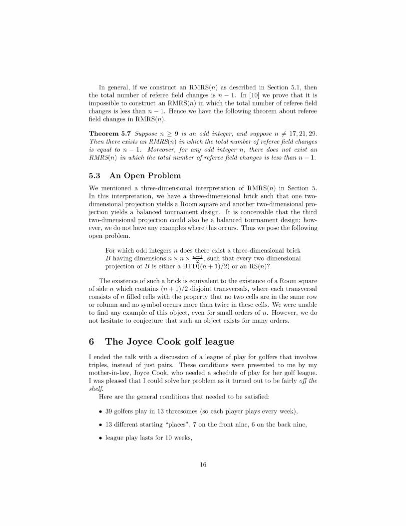
In general, if we construct an RMRS(n) as described in Section 5.1, thenthe total number of referee field changes is n − 1. In [10] we prove that it isimpossible to construct an RMRS(n) in which the total number of referee fieldchanges is less than n − 1. Hence we have the following theorem about refereefield changes in RMRS(n).

Theorem 5.7 Suppose n ≥ 9 is an odd integer, and suppose n 6= 17, 21, 29.Then there exists an RMRS(n) in which the total number of referee field changesis equal to n − 1. Moreover, for any odd integer n, there does not exist anRMRS(n) in which the total number of referee field changes is less than n − 1.

5.3 An Open Problem

We mentioned a three-dimensional interpretation of RMRS(n) in Section 5.In this interpretation, we have a three-dimensional brick such that one two-dimensional projection yields a Room square and another two-dimensional pro-jection yields a balanced tournament design. It is conceivable that the thirdtwo-dimensional projection could also be a balanced tournament design; how-ever, we do not have any examples where this occurs. Thus we pose the followingopen problem.

For which odd integers n does there exist a three-dimensional brickB having dimensions n× n × n+1

2, such that every two-dimensional

projection of B is either a BTD((n + 1)/2) or an RS(n)?

The existence of such a brick is equivalent to the existence of a Room squareof side n which contains (n + 1)/2 disjoint transversals, where each transversalconsists of n filled cells with the property that no two cells are in the same rowor column and no symbol occurs more than twice in these cells. We were unableto find any example of this object, even for small orders of n. However, we donot hesitate to conjecture that such an object exists for many orders.

6 The Joyce Cook golf league

I ended the talk with a discussion of a league of play for golfers that involvestriples, instead of just pairs. These conditions were presented to me by mymother-in-law, Joyce Cook, who needed a schedule of play for her golf league.I was pleased that I could solve her problem as it turned out to be fairly off theshelf.

Here are the general conditions that needed to be satisfied:

• 39 golfers play in 13 threesomes (so each player plays every week),

• 13 different starting “places”, 7 on the front nine, 6 on the back nine,

• league play lasts for 10 weeks,

16

Here are the balance conditions:

• no two golfers are together in a threesome more than once,

• no golfer starts in the same place twice.

First note that since each golfer plays with two other golfers per week andthere are 10 weeks, that each golfer only plays with 20 of the 38 other golfers,so the tournament schedule is not particularly tight.

In order to construct this schedule we need another object from combinato-rial design theory called a latin square.

Definition A latin square of side (order) n is an n× n array in which each cellcontains a single element from an n−set S, and such that each element occursexactly once in each row and exactly once in each column.

Example 6.1 A latin square L of side 3 on symbol set S = {1, 2, 3}.

L =1 2 32 3 13 1 2

We note in passing that the existence of a latin square of side n is equivalentto the the existence of a bipartite tournament schedule for two teams each withn players. The rows represent one team, the columns represent the other teamand the cells represent the rounds. More specifically, if L(r, c) = s, then personr from team 1 plays person c from team 2 in round s.

Definition Two latin squares L and R (both on the symbol set S) of the sameorder are orthogonal if when superimposed, every ordered pair of symbols fromS × T occurs exactly once.

Example 6.2 Two orthogonal latin squares L and R of side 3 on symbol setS = {1, 2, 3} and the resulting superimposed square L × R.

L =1 2 32 3 13 1 2

R =1 2 33 1 22 3 1

L × R =1,1 2,2 3,32,3 3,1 1,23,2 1,3 2,1

Orthogonal latin squares have been studied since they were first constructedby Euler in 1782 in an attempt to solve the 36 officer problem. There is extensiveliterature on Latin squares and the interested reader is referred to [5] and to[3] (Part 2). One of the primary questions in this area concerns the existenceof sets of pairwise orthogonal latin squares for each order n. It is not hardto show that there are at most n − 1 pairwise orthogonal latin squares of side

17

n. However, this upper bound has only been achieved in the case when n is aprime power. Nonetheless, this will be sufficient for our purposes. We have thefollowing theorem in this case.

Theorem 6.3 When n is a prime power, there exist n− 1 pairwise orthogonallatin squares of side n.

We solve our golf scheduling problem by the use of 3 pairwise orthogonallatin squares of side 13. We denote these as A, B and C. These three squaresare given in Example 6.4.

Example 6.4 Three pairwise orthogonal latin squares of side 13.

A =

0 1 2 3 4 5 6 7 8 9 10 11 121 2 3 4 5 6 7 8 9 10 11 12 02 3 4 5 6 7 8 9 10 11 12 0 13 4 5 6 7 8 9 10 11 12 0 1 24 5 6 7 8 9 10 11 12 0 1 2 35 6 7 8 9 10 11 12 0 1 2 3 46 7 8 9 10 11 12 0 1 2 3 4 57 8 9 10 11 12 0 1 2 3 4 5 68 9 10 11 12 0 1 2 3 4 5 6 79 10 11 12 0 1 2 3 4 5 6 7 810 11 12 0 1 2 3 4 5 6 7 8 911 12 0 1 2 3 4 5 6 7 8 9 1012 0 1 2 3 4 5 6 7 8 9 10 11

B =

0 1 2 3 4 5 6 7 8 9 10 11 122 3 4 5 6 7 8 9 10 11 12 0 14 5 6 7 8 9 10 11 12 0 1 2 36 7 8 9 10 11 12 0 1 2 3 4 58 9 10 11 12 13 1 2 3 4 5 6 710 11 12 0 1 2 3 4 5 6 7 8 912 0 1 2 3 4 5 6 7 8 9 10 111 2 3 4 5 6 7 8 9 10 11 12 03 4 5 6 7 8 9 10 11 12 0 1 25 6 7 8 9 10 11 12 0 1 2 3 47 8 9 10 11 12 0 1 2 3 4 5 69 10 11 12 0 1 2 3 4 5 6 7 811 12 0 1 2 3 4 5 6 7 8 9 10

18

C =

0 1 2 3 4 5 6 7 8 9 10 11 123 4 5 6 7 8 9 10 11 12 0 1 26 7 8 9 10 11 12 0 1 2 3 4 59 10 11 12 0 1 2 3 4 5 6 7 812 0 1 2 3 4 5 6 7 8 9 10 112 3 4 5 6 7 8 9 10 11 12 0 15 6 7 8 9 10 11 12 0 1 2 3 48 9 10 11 12 0 1 2 3 4 5 6 711 12 0 1 2 3 4 5 6 7 8 9 101 2 3 4 5 6 7 8 9 10 11 12 04 5 6 7 8 9 10 11 12 0 1 2 37 8 9 10 11 12 0 1 2 3 4 5 610 11 12 0 1 2 3 4 5 6 7 8 9

Now we can solve our golf scheduling problem. We superimpose these threesquares to make a 13×13 array S: Each cell of S contains a triple (i, j, k) wherei is from A, j is from B, and k is from C. Our 39 golfers consist of the 13symbols from A plus the 13 symbols from B plus the 13 symbols from C. Welet the weeks of the tournament be the rows of S and the 13 different startingplaces be the columns. (Note that we even have 3 extra weeks). If the triple inrow r, column c is (i, j, k), then in week r, the triple consisting of golfer i (fromthe A group) and golfer j (from the B group) and golfer k (from the C group)will start at place c.

In Example 6.5 below we give the first three weeks of the tournament. Wecan observe that in week 3, player 2 from A and player 4 from B and player 3from C form a threesome what starts at place 1 (probably hole #1).

Example 6.5 The first 3 weeks of the tournament for 39 golfers (we have re-placed 10 by a, 11 by b and 12 by c and supressed all commas) .

S =000 111 222 333 444 555 666 777 888 999 aaa bbb ccc

123 234 345 456 567 678 789 89a 9ab abc bc0 c01 012246 357 468 579 68a 79b 8ac 9b0 ac1 b02 c13 024 135

We now check the conditions. Obviously there are 39 players playing inthreesomes. There are also 13 different starting places and the league play isdesigned for 10 weeks (with three extra weeks possible). From the fact thatA, B and C are latin squares we have that each player plays once in each weekand that no golfer starts in the same place twice. From the fact that these latinsquares are orthogonal we have that no two golfers are together in a threesomemore than once. Thus we have our schedule.

7 Further information

Further information on our scheduling of the XFL can be found at [7]. Astreaming video of parts of this talk as well as many of the slides from this talk

19

can be found at www.msri.org/publications/ln/msri/2000/combdes/dinitz/1/.A discussion of tournament scheduling that pays particular attention to thehome-away patterns can be found at [1]. An extensive survey of Room squaresand related designs (including balanced tournament designs) is [9]. Finally, asnoted above there is extensive literature on Latin squares and the interestedreader is referred to [5] and to [3] (Part 2).

Large schedules such as Major League Baseball require integer programmingtechniques from operations research. These methods are beyond the scope ofthis talk, however the interested reader is referred to the web page of MichaelTrick (http://mat.tepper.cmu.edu/sports/) for further information on this typeof scheduling.

References

[1] E. Burke, D. de Werra, J. Kingston, Applications to timetabling, in Hand-book of Graph Theory (J. Gross and J. Yellen, eds.) CRC Press, 2004,pp.445 - 474.

[2] P. Cohen, What good is math? An answer for jocks. New York Times(Feb. 3, 2001) (National Ed.) pp. A15, A17.

[3] C. J. Colbourn and J. H. Dinitz, eds. The CRC Handbook of CombinatorialDesigns, CRC Press, Inc., 1996.

[4] J. Corriveau, Enumeration of balanced tournament designs. Ars Combin25 (1988), 93–105.

[5] J. Denes and A. D. Keedwell, Latin squares and their applications, Aca-demic Press, New York-London, 1974, 547 pp.

[6] J. H. Dinitz and M. H. Dinitz, Enumeration of balanced tournament de-signs 10 points, J. Combin. Math. Combin. Comput., to appear.

[7] J. H. Dinitz and D. Froncek, Scheduling the XFL, Congr. Numer. 147(2000), pp. 5 – 15.

[8] J. H. Dinitz, D. K. Garnick and B. D. McKay, There are 526, 915, 620nonisomorphic one-factorizations of K12. J. Combin. Des. 2 (1994), 273–285.

[9] J. H. Dinitz and D. R. Stinson. Room squares and related designs. InContemporary Design Theory: A Collection of Surveys, John Wiley &Sons, Inc., 1992, pp. 137–204.

[10] J. H. Dinitz and D. R. Stinson, On assigning referees to tournament sched-ules, Bull. Inst. Combin. and its Appl., to appear.

[11] K. B. Gross, R. C. Mullin and W. D. Wallis, The number of pairwiseorthogonal symmetric Latin squares, Util. Math. 4 (1973), 239–251.

20

[12] J. Haselgrove and J. Leach, A tournament design problem Amer. MathMonthly, March 1977, 198 – 201

[13] E. R. Lamken, S. A. Vanstone, The existence of partitioned balancedtournament designs. in Combinatorial design theory, North-Holland Math.Stud., 149, North-Holland, Amsterdam, 1987. 339–352,

[14] E. R. Lamken. A few more partitioned balanced tournament designs. ArsCombinatoria 43 (1996), 121–134.

[15] E. R. Lamken and S. A. Vanstone. Balanced tournament designs andrelated topics. Discrete Math. 77 (1989), 159–176.

[16] E. Mendelsohn and P. Rodney, Mendelsohn, The existence of court bal-anced tournament designs, Discrete Math. 133 (1994), 207–216.

[17] R. C. Mullin and W. D. Wallis. The existence of Room squares. Aequa-tiones Math. 13 (1975), 1–7.

[18] P. J. Schellenberg, G. H. J. van Rees and S. A. Vanstone. The existenceof balanced tournament designs. Ars Combin. 3 (1977), 303–318.

[19] D. R. Stinson. Room squares with maximum empty subarrays. Ars Com-bin. 20 (1985), 159–166.

21