DESIGN AND MODELING OF ADAPTIVE CRUISE CONTROL SYSTEM ...
86
DESIGN AND MODELING OF ADAPTIVE CRUISE CONTROL SYSTEM USING PETRI NETS WITH FAULT TOLERANCE CAPABILITIES A Thesis Submitted to the Faculty of Purdue University by Nivethitha Amudha Chandramohan In Partial Fulfillment of the Requirements for the Degree of Master of Science in Electrical and Computer Engineering May 2018 Purdue University Indianapolis, Indiana
Transcript of DESIGN AND MODELING OF ADAPTIVE CRUISE CONTROL SYSTEM ...
DESIGN AND MODELING OF ADAPTIVE CRUISE CONTROL SYSTEM
USING PETRI NETS WITH FAULT TOLERANCE CAPABILITIES
A Thesis
Submitted to the Faculty
of
Purdue University
by
Nivethitha Amudha Chandramohan
In Partial Fulfillment of the
Requirements for the Degree
of
Master of Science in Electrical and Computer Engineering
May 2018
Purdue University
Indianapolis, Indiana
ii
THE PURDUE UNIVERSITY GRADUATE SCHOOL
STATEMENT OF COMMITTEE APPROVAL
Dr. Lingxi Li, Chair
Department of Electrical and Computer Engineering
Dr. Yaobin Chen
Department of Electrical and Computer Engineering
Dr. Brian King
Department of Electrical and Computer Engineering
Approved by:
Dr. Brian King
Head of the Graduate Program

iii
This research is dedicated to all who loved, supported and believed in me

iv
ACKNOWLEDGMENTS
I would like to dedicate this work to my father Dr. M. Chandramohan, mother
Dr. T. Amudha and my sister Sree Narmadha for their love and affection and for
their encouragement to pursue my dreams in USA. I would like to extend my hearty
thanks to my advisor Dr. Lingxi Li for creating a platform to learn and explore in
the automotive industry. It might not be possible without his encouragement and
guidance throughout my masters at IUPUI. I would like to thank my committee
members Dr. Brian King and Dr. Yaobin Chen for their valuable comments and
support. I am thankful to Sherrie Tucker for her timely help during deadlines and
for her great work during the documentation of my thesis. Many thanks to my
friends Gokul Das, Bala Sai Varma and Avinash for their assistance, timely help in
analyzing the model and moral support. Sweet thanks to Vani for helping me in
documentation. I thank all my friends for being patient and helpful during the final
stage of submission. A special thanks to my Cummins team for their support and
understanding.

v
TABLE OF CONTENTS
Page
LIST OF TABLES . . . . . . . . . . . . . . . . . . . . . . . . . . . . . . . . . . vii
LIST OF FIGURES . . . . . . . . . . . . . . . . . . . . . . . . . . . . . . . . . viii
SYMBOLS . . . . . . . . . . . . . . . . . . . . . . . . . . . . . . . . . . . . . . ix
ABBREVIATIONS . . . . . . . . . . . . . . . . . . . . . . . . . . . . . . . . . . x
ABSTRACT . . . . . . . . . . . . . . . . . . . . . . . . . . . . . . . . . . . . . xii
1 INTRODUCTION . . . . . . . . . . . . . . . . . . . . . . . . . . . . . . . . 1
1.1 Literature review . . . . . . . . . . . . . . . . . . . . . . . . . . . . . . 2
1.2 Contributions . . . . . . . . . . . . . . . . . . . . . . . . . . . . . . . . 7
1.3 Organization . . . . . . . . . . . . . . . . . . . . . . . . . . . . . . . . 7
2 PETRI NETS . . . . . . . . . . . . . . . . . . . . . . . . . . . . . . . . . . . 9
2.1 Petri Net Marking Scheme . . . . . . . . . . . . . . . . . . . . . . . . 11
2.2 Petri Nets Dynamics . . . . . . . . . . . . . . . . . . . . . . . . . . . . 13
2.3 Petri Nets State Equation . . . . . . . . . . . . . . . . . . . . . . . . . 16
2.4 Continuous Petri Nets . . . . . . . . . . . . . . . . . . . . . . . . . . . 18
2.5 Hybrid Petri Nets . . . . . . . . . . . . . . . . . . . . . . . . . . . . . . 21
3 ADAPTIVE CRUISE CONTROL SYSTEM IMPLEMENTATION . . . . . . 25
3.1 Definition . . . . . . . . . . . . . . . . . . . . . . . . . . . . . . . . . . 25
3.2 Adaptive Cruise Control system interface . . . . . . . . . . . . . . . . . 26
3.2.1 Control Unit . . . . . . . . . . . . . . . . . . . . . . . . . . . . . 26
3.2.2 Sensors . . . . . . . . . . . . . . . . . . . . . . . . . . . . . . . . 27
3.2.3 Communication Protocol . . . . . . . . . . . . . . . . . . . . . . 30
3.3 Feature implementation by OEMs . . . . . . . . . . . . . . . . . . . . . 30
3.4 Model of Adaptive cruise control in Discrete Petri net . . . . . . . . . . 31
3.4.1 Version 1 . . . . . . . . . . . . . . . . . . . . . . . . . . . . . . 31
vi
Page
3.4.2 Version 2 . . . . . . . . . . . . . . . . . . . . . . . . . . . . . . 35
3.4.3 Drawbacks . . . . . . . . . . . . . . . . . . . . . . . . . . . . . . 38
3.5 Final updated model . . . . . . . . . . . . . . . . . . . . . . . . . . . . 39
3.6 Invariant Analysis . . . . . . . . . . . . . . . . . . . . . . . . . . . . . . 46
3.6.1 Place invariant . . . . . . . . . . . . . . . . . . . . . . . . . . . 49
3.6.2 Transition Invariant: . . . . . . . . . . . . . . . . . . . . . . . . 49
3.6.3 Reachability states . . . . . . . . . . . . . . . . . . . . . . . . . 52
4 CONTROLLER AND FAULT TOLERANCE . . . . . . . . . . . . . . . . . 56
4.1 Controller . . . . . . . . . . . . . . . . . . . . . . . . . . . . . . . . . . 56
4.2 Fault tolerance Techniques . . . . . . . . . . . . . . . . . . . . . . . . . 61
4.2.1 Separate Redundant Petri Net Controllers . . . . . . . . . . . . 61
4.2.2 Fault Detection and Identification . . . . . . . . . . . . . . . . . 62
4.2.3 Detection and Identification of a Single Place Fault . . . . . . . 63
4.3 Failure cases . . . . . . . . . . . . . . . . . . . . . . . . . . . . . . . . . 66
4.3.1 Failure due to Driver response or hardware . . . . . . . . . . . 66
4.3.2 Model failure . . . . . . . . . . . . . . . . . . . . . . . . . . . . 67
5 CONCLUSION AND FUTURE WORK . . . . . . . . . . . . . . . . . . . . 69
5.1 Conclusion . . . . . . . . . . . . . . . . . . . . . . . . . . . . . . . . . . 69
5.2 Future Work . . . . . . . . . . . . . . . . . . . . . . . . . . . . . . . . . 69
5.2.1 Hybrid PetriNet model Integration . . . . . . . . . . . . . . . . 69
5.2.2 SimHPN tool . . . . . . . . . . . . . . . . . . . . . . . . . . . . 70
5.2.3 Interface with other safety features . . . . . . . . . . . . . . . . 70
REFERENCES . . . . . . . . . . . . . . . . . . . . . . . . . . . . . . . . . . . . 71
vii
LIST OF TABLES
Table Page
3.2 Transitions in ACC model . . . . . . . . . . . . . . . . . . . . . . . . . . . 42
3.1 Places in the model . . . . . . . . . . . . . . . . . . . . . . . . . . . . . . . 44
viii
LIST OF FIGURES
Figure Page
2.1 Graphical representation of Petri nets . . . . . . . . . . . . . . . . . . . . . 9
2.2 Petri Net model- An Example . . . . . . . . . . . . . . . . . . . . . . . . . 12
2.3 Example to depict Petri net dynamics . . . . . . . . . . . . . . . . . . . . 13
2.4 Reachability Tree for Petri Net model . . . . . . . . . . . . . . . . . . . . . 15
2.5 Example for Continuous Petri Net . . . . . . . . . . . . . . . . . . . . . . . 19
2.6 Reachability Graph for a Continuous Petri Net using Macro-Markings . . . 21
2.7 Example for Hybrid Petri Net Model . . . . . . . . . . . . . . . . . . . . . 24
3.1 ACC Concept . . . . . . . . . . . . . . . . . . . . . . . . . . . . . . . . . . 25
3.2 Interface of ACC system with the modules . . . . . . . . . . . . . . . . . . 28
3.3 Flow Chart of Version 1 . . . . . . . . . . . . . . . . . . . . . . . . . . . . 32
3.4 Petri Net model of Version 1 . . . . . . . . . . . . . . . . . . . . . . . . . . 34
3.5 Flow Chart of Version 2 . . . . . . . . . . . . . . . . . . . . . . . . . . . . 36
3.6 Petri Net model of Version 2 . . . . . . . . . . . . . . . . . . . . . . . . . . 37
3.7 Algorithm of ACC . . . . . . . . . . . . . . . . . . . . . . . . . . . . . . . 40
3.8 Final model of ACC . . . . . . . . . . . . . . . . . . . . . . . . . . . . . . 41
3.9 Reachability States . . . . . . . . . . . . . . . . . . . . . . . . . . . . . . . 55
4.1 ACC Model with Controller . . . . . . . . . . . . . . . . . . . . . . . . . . 57
4.2 ACC Reachability Controller Manual AccelerationEnabled . . . . . . . . . 59
4.3 ACC Reachability Controller Manual BrakingEnabled . . . . . . . . . . . . 60
4.4 ACC Model with Redundant Controller places . . . . . . . . . . . . . . . . 65

ix
SYMBOLS
m mass
v velocity
d distance
t time
V voltage
Mph miles per hour
f frequency
m/s meter/second

x
ABBREVIATIONS
CC Cruise Control
ADAS Advanced Driver Assistant System
ACC Adaptive Cruise Control
CACC Co-operative Adaptive Cruise Control
RADAR Radio Detection and Ranging
MPC Model Predictive Control
KDE Kernel Density Estimation
PDF Probability Density Function
ABS Anti-lock Braking System
ECC Eco Cruising Control
Thw Time head way
NPC Non-linear Predictive Control
SOS System of Systems
HMI Human Machine Interface
DSC Distance Control Status
SS Speed Status
GSPI Gain Scheduling Proportional Integral
GSLQ Gain Scheduling Linear Quadratic
IIO Incremental Input Output
GIS Geographic Information System
GPS Global Positioning System
SVM Support Vector Machine
CAN Control Area Network
HLC High Level Control

xi
mph Miles per hour
CG Center of Gravity
AEB Automatic Emergency Braking
xii
ABSTRACT
Amudha Chandramohan, Nivethitha. M.S.E.C.E., Purdue University, May 2018. De-sign and Modeling of Adaptive Cruise Control System Using Petri Nets with FaultTolerance Capabilities. Major Professor: Lingxi Li.
In automotive industry, driver assistance and active safety features are main areas
of research. This thesis concentrates on designing one of the famous ADAS system
feature called Adaptive cruise control. Feature development and analysis of various
functionalities involved in the system control are done using Petri Nets. A background
on the past and current ACC research is noted and taken as motivation. The idea
is to implement the adaptive cruise control system in Petri net and analyze how to
provide fault tolerance to the system. The system can be evaluated for various cases.
The ACC technology implemented in different cars were compared and discussed.
The interaction of the ACC module with other modules in the car is explained. The
cruise system’s algorithm in Petri net is used as the basis for developing Adaptive
Cruise Control system’s algorithm. The ACC system model is designed using Petri
nets and various Petri net functionalities like place invariant, transition invariant and
reachability tree of the model are analyzed. The results are verified using Matlab.
Controllers are introduced for ideal cases and are implemented in Petri nets. Then
the error cases are considered and fault tolerance techniques are carried out on the
model to identify the fault places.

1
1. INTRODUCTION
With the increasing demand for car and road safety, there is a necessity for a sys-
tem that can effectively monitor the controls and assist in driving. Advanced driver
assistance systems (ADAS) aims to utilize the available human-machine interface to
improve car safety. ADAS provides important and critical information to the driver,
automates tasks that require extreme human precision with the goal of inciting road
safety. ADAS technologies are currently contributing to reduction in the number of
crashes and casualties thereby creating high expectations in the future. With the
exponential rise in the number of vehicles, the need for an in-vehicle ADAS system is
also rising exponentially. Adaptive cruise control, anti-lock braking, automatic park-
ing, pedestrian protection system, blind spot detection are some examples of ADAS
already in use. Cruise control is a servomechanism system used to maintain the speed
of a vehicle set by the driver. The throttle pedal of the car is taken over by the cruise
control system to maintain a steady speed. The cruise control system had its roots
way back in 1940s, when there emerged an idea of manipulating the speed of a car
using an electrically controlled device. Instead of the pedal press, the cruise control
systems sought to operate the throttle by a cable connected to an actuator which
would in turn control the acceleration of the car. However, blind implementation of
cruise control without taking into consideration certain environmental and circum-
stantial factors led to undesirable operations causing it to become obsolete. In order
to accommodate these factors into the cruise control, improved strategies known as
Adaptive Cruise Control or autonomous cruise control were developed.
Adaptive cruise control is a type of ADAS which regulates the speed of the car
causing the vehicle to maintain a safe distance from the vehicles ahead. The efficacy
of the system can be seen especially on highways where the driver must continuously
monitor their cruise control for their own safety. With the use of adaptive cruise con-
2
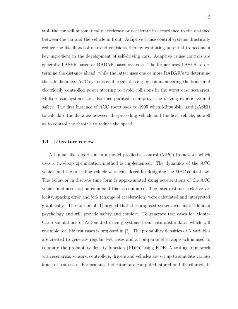
trol, the car will automatically accelerate or decelerate in accordance to the distance
between the car and the vehicle in front. Adaptive cruise control systems drastically
reduce the likelihood of rear end collisions thereby exhibiting potential to become a
key ingredient in the development of self-driving cars. Adaptive cruise controls are
generally LASER-based or RADAR-based systems. The former uses LASER to de-
termine the distance ahead, while the latter uses one or more RADAR’s to determine
the safe distance. ACC systems enable safe driving by commandeering the brake and
electrically controlled power steering to avoid collisions in the worst case scenarios.
Multi-sensor systems are also incorporated to improve the driving experience and
safety. The first instance of ACC roots back to 1995 when Mitsubishi used LASER
to calculate the distance between the preceding vehicle and the host vehicle, as well
as to control the throttle to reduce the speed.
1.1 Literature review
A human like algorithm in a model predictive control (MPC) framework which
uses a two-loop optimization method is implemented. The dynamics of the ACC
vehicle and the preceding vehicle were considered for designing the MPC control law.
The behavior in discrete time form is approximated using accelerations of the ACC
vehicle and acceleration command that is computed. The inter-distance, relative ve-
locity, spacing error and jerk (change of acceleration) were calculated and interpreted
graphically. The author of [1] argued that the proposed system will match human
psychology and will provide safety and comfort. To generate test cases for Monte-
Carlo simulations of Automated driving systems from naturalistic data, which will
resemble real life test cases is proposed in [2]. The probability densities of N variables
are created to generate regular test cases and a non-parametric approach is used to
compute the probability density function (PDFs) using KDE. A testing framework
with scenarios, sensors, controllers, drivers and vehicles are set up to simulate various
kinds of test cases. Performance indicators are computed, stored and distributed. It
3
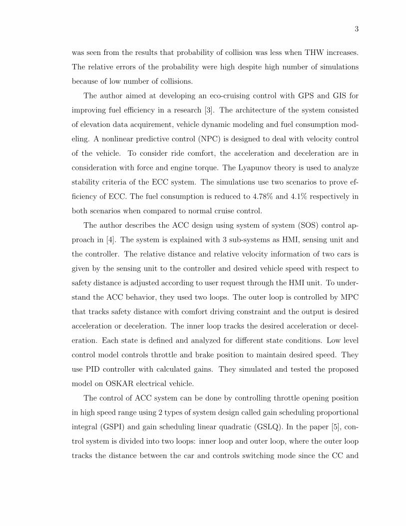
was seen from the results that probability of collision was less when THW increases.
The relative errors of the probability were high despite high number of simulations
because of low number of collisions.
The author aimed at developing an eco-cruising control with GPS and GIS for
improving fuel efficiency in a research [3]. The architecture of the system consisted
of elevation data acquirement, vehicle dynamic modeling and fuel consumption mod-
eling. A nonlinear predictive control (NPC) is designed to deal with velocity control
of the vehicle. To consider ride comfort, the acceleration and deceleration are in
consideration with force and engine torque. The Lyapunov theory is used to analyze
stability criteria of the ECC system. The simulations use two scenarios to prove ef-
ficiency of ECC. The fuel consumption is reduced to 4.78% and 4.1% respectively in
both scenarios when compared to normal cruise control.
The author describes the ACC design using system of system (SOS) control ap-
proach in [4]. The system is explained with 3 sub-systems as HMI, sensing unit and
the controller. The relative distance and relative velocity information of two cars is
given by the sensing unit to the controller and desired vehicle speed with respect to
safety distance is adjusted according to user request through the HMI unit. To under-
stand the ACC behavior, they used two loops. The outer loop is controlled by MPC
that tracks safety distance with comfort driving constraint and the output is desired
acceleration or deceleration. The inner loop tracks the desired acceleration or decel-
eration. Each state is defined and analyzed for different state conditions. Low level
control model controls throttle and brake position to maintain desired speed. They
use PID controller with calculated gains. They simulated and tested the proposed
model on OSKAR electrical vehicle.
The control of ACC system can be done by controlling throttle opening position
in high speed range using 2 types of system design called gain scheduling proportional
integral (GSPI) and gain scheduling linear quadratic (GSLQ). In the paper [5], con-
trol system is divided into two loops: inner loop and outer loop, where the outer loop
tracks the distance between the car and controls switching mode since the CC and

4
ACC are controlled by switching mode. The inner loop acting as a velocity tracking
controller, controls the brake position and the throttle position according to the vary-
ing speed. They used a vehicle model to explain the relation between engine speed,
inertia, engine torque and various parameters that effect speed and distance of the
vehicle. They used a look up table that includes engine torque vs engine rotation
speed and percentage of throttle opening position. The desired distance headway is
calculated using an equation called ’constant time headway policy. They have tested
models in three scenarios as velocity tracking, distance tracking and switching mode,
and simulated the results.
The position control algorithm can be used to control acceleration pedal and brake
pedal by directly using DC servo motor. The two modes of control used by author
Pananurak and his colleges in [6] are velocity and distance control. The low speed
ACC is operated at very low speed approximately 5km/hr and stopping and restarting
of vehicle is needed for motion of the vehicle. The inputs of fuzzy controller are relative
velocity and distance error and the outputs are braking and velocity command. The
distance sensor used is laser range finder, SICK LMS 291 and it is placed in the
bumper. To calculate distance between the object and sensor, elapse time between
transmitting and receiving of laser pulse is used. Digital low pass filter is used to
filter noise in the velocity signal. For distance control experiment, fuzzy parameters
are adjusted in the algorithm according to responses from the vehicle.
In an ADAS technology with an autonomous control system architecture they have
created an intelligent ACC system consisting of three important parts in [4]. High
level control, low level control and sensor unit subsystem. Each has a state machine
to control the unit. The HLC state machine consist of 4 states according to which the
system operates. ACC off state, distance control state, Pass state and cruise control
state. Each state has a certain condition to function and the combination of various
states is the ACC control system. It is basically a PID controller designed and tested
on an electrical vehicle. So, the ACC system has SOS based control architecture.
5
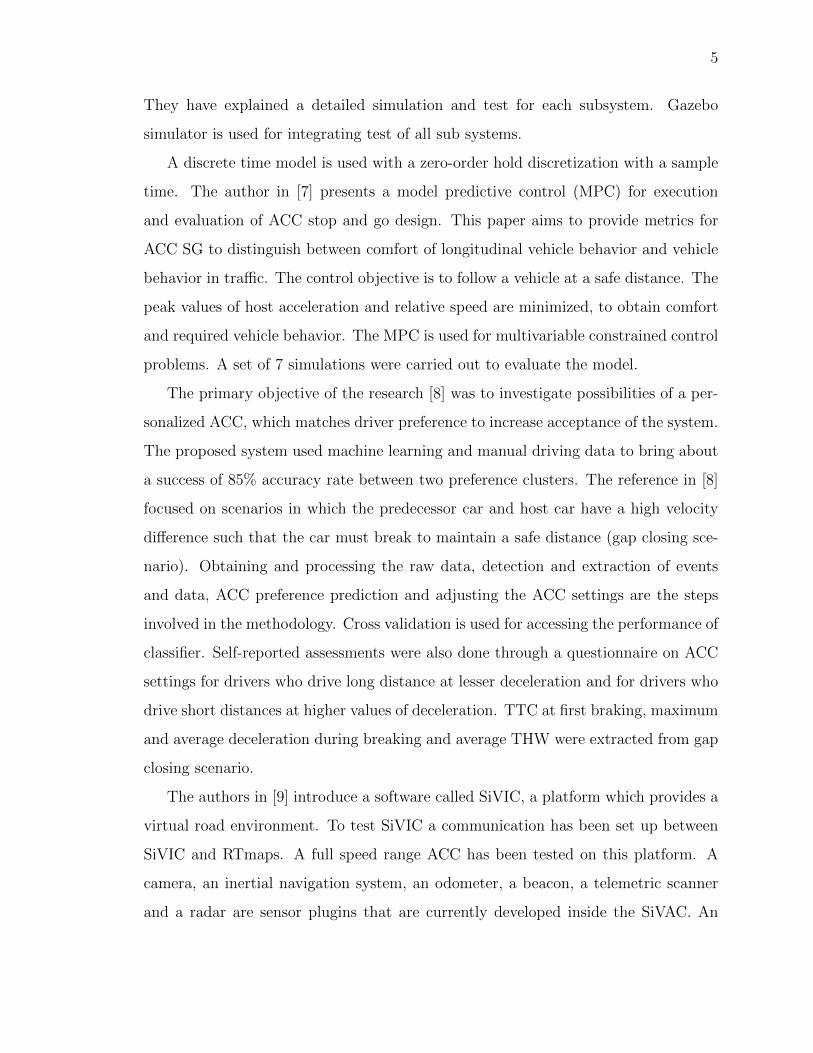
They have explained a detailed simulation and test for each subsystem. Gazebo
simulator is used for integrating test of all sub systems.
A discrete time model is used with a zero-order hold discretization with a sample
time. The author in [7] presents a model predictive control (MPC) for execution
and evaluation of ACC stop and go design. This paper aims to provide metrics for
ACC SG to distinguish between comfort of longitudinal vehicle behavior and vehicle
behavior in traffic. The control objective is to follow a vehicle at a safe distance. The
peak values of host acceleration and relative speed are minimized, to obtain comfort
and required vehicle behavior. The MPC is used for multivariable constrained control
problems. A set of 7 simulations were carried out to evaluate the model.
The primary objective of the research [8] was to investigate possibilities of a per-
sonalized ACC, which matches driver preference to increase acceptance of the system.
The proposed system used machine learning and manual driving data to bring about
a success of 85% accuracy rate between two preference clusters. The reference in [8]
focused on scenarios in which the predecessor car and host car have a high velocity
difference such that the car must break to maintain a safe distance (gap closing sce-
nario). Obtaining and processing the raw data, detection and extraction of events
and data, ACC preference prediction and adjusting the ACC settings are the steps
involved in the methodology. Cross validation is used for accessing the performance of
classifier. Self-reported assessments were also done through a questionnaire on ACC
settings for drivers who drive long distance at lesser deceleration and for drivers who
drive short distances at higher values of deceleration. TTC at first braking, maximum
and average deceleration during breaking and average THW were extracted from gap
closing scenario.
The authors in [9] introduce a software called SiVIC, a platform which provides a
virtual road environment. To test SiVIC a communication has been set up between
SiVIC and RTmaps. A full speed range ACC has been tested on this platform. A
camera, an inertial navigation system, an odometer, a beacon, a telemetric scanner
and a radar are sensor plugins that are currently developed inside the SiVAC. An
6
application to SiVAC is a full speed range ACC. The authors goal is to control vehicle
speed at a desired speed and scenario. An overview of the application with SiVIC
vehicles, sensors and RTMap was observed in this paper. A graphical representation
of distance between the vehicles, speed references and speed profiles of preceding and
leading vehicles were also recognized.
The confusion in modes due to human interaction is caused due to reasons such
as misunderstanding of the behavior by the driver, unnecessary complex automation
along with poor display of the state is discussed in [10]. To battle the above issues, a
new interface methodology was developed for ACC systems. Models of the machine
and interface are developed. The traditional interface model has three modes which
has been proven to cause high confusion due to incompatibility issues. Thereby, the
four mode interface models was utilized as a baseline to improve the performance.
Graphical user interface was implemented using a gauge clutter and was heavily based
on the ones made by major names in the automobile industry. Another interesting
observation was made in four and five mode models that the confusion occurred due
to the similarity in color between two consecutive states. The solution was to merge
both states that reduces the amount of confusion or surprise by the user.
A methodology by modeling and simulating cars having both V2V and ACC on
three simulation scenarios to improve road safety is explained in [11] The platform
used for simulation are SUMO and Scene Suite. The goals of the paper are to deter-
mine the main effects of low penetration rate of ADAS-ACC and V2V communication
alone. The three phases of the proposed architecture are Specification and require-
ments, Modeling and simulation, and analysis and verification. Under specification
and requirements, three different scenarios were developed to determine the imple-
mentation of the combination of V2V and ACC. The combination of ACC and V2V
in comparison to ACC alone with a 40% and 60% penetration rate showed that, the
former prevented all types of accidents including side and read end collisions.
7
The advantages of Petri nets are:
• Linear-algebraic techniques can also be used to analyze the behavior of Petri
nets.
• The concept of place-invariant is useful in that regard.
• Efficient techniques for extremely large systems.
• Modeling and analysis is easy.
• Discrete event systems simulation techniques on low cost platforms.
• Fault tolerance and security.
• Computational complexity.
1.2 Contributions
The contributions of this thesis are summarized as follows:
• Designed a control algorithm for Adaptive Cruise Control.
• Modeled the Adaptive cruise control in Petri Nets.
• Analyzed of the functionality of Petri nets.
• Verified the Adaptive cruise control process.
• Implemented controller and Fault tolerance techniques.
1.3 Organization
This Thesis seeks to design Adaptive cruise control strategy by employing Petri
net control system and analyze the model with fault tolerance techniques. Chapter
2 explains the Petri nets concepts followed by Chapter 3 describing about various
versions of ACC models in Petri net with their drawbacks and the derived final petri

8
net model rectifying all the observed drawbacks and the invariant analysis Chapter
4 describes the controller and fault tolerance techniques and Chapter 5 presents the
conclusion and future work.
9
2. PETRI NETS
Petri nets are mathematical representations for modeling any day-to-day applications
or life scenarios as discrete, continuous or hybrid systems or processes. These mod-
eling tools are also called Place-Transition net that helps to represents various event
or time based processes. Petri nets are known as weighted bipartite directed graph
consisting of nodes and vertices called places and transitions respectively, which are
inter-connected via arcs. The circles in model represents the places (concentric circles
in case of a continuous system) and transitions are portrayed using thin rectangular
bars opaque for discrete and transparent for continuous models. Arcs connect a
transition to places or a place to transitions only and have a finite weight which are
positive real numbers. The weight of any arc is equal to one, if the weights are not
explicitly shown in the graphical representation. Also, for any given Petri net model,
the graphical representation always have a finite number of places and transitions.
The Petri net model was used to depict complex control systems and algorithms was
invented by Carl Adam in the 1960s [12] to represent chemical processes.
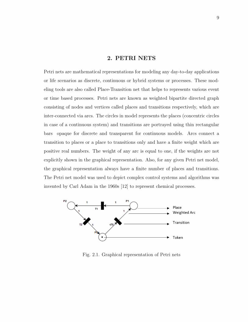
Fig. 2.1. Graphical representation of Petri nets

10
A typical example for a Petri net is as shown above. Various parts of a Petri net
is also marked to get a better understanding of the same. Mathematically a Petri net
graph is represented as follows,
PN = {P, T,A,w} (2.1)
where, P , represents the set of finite Places in the Petri net model. Shown as
circles in the above model. A model with N places is represented as,
P = {P0, P1, P2, ....P (N − 1)} (2.2)
T , represents the set of finite Transitions in the petri net model. Shown as the
bars in the above model. A model with M transitions is represented as,
T = {T0, T1, T2, ....T (M − 1)} (2.3)
A, represents set of all arcs from P to T (places to transitions) and T to P (tran-
sitions to places). A model with N places and M transitions is represented with arcs
as follows,
A ⊆ ( P × T ) ∪ ( T × P ) (2.4)
w represents the weights carried by each arcs depicted in the Petri net model.
As mentioned above, if no weights has been explicitly depicted, it means it carries a
weight of one. Mathematically it is represented as,
w = {1, 2, 3, 4, ..} (2.5)
Apart from these notations, the set of arcs, A is represented using matrix form
using the input incident matrix and output incident matrix to simplify the mathe-
matical calculations associated with petri nets. B− being the input incident matrix,
which constitute the arc weights of edges directed from places transitions ( P × T ) .
The weight of an arc from place Pi to transition Tj is represented as w(Pi, T j) of
matrix, B−[B−(Pi, T j) ] captures the output incident matrix, which constitute the
arc weights of edges directed from transitions to places. The weight of an arc from
11
transition T j to place P i is represented as w(Tj, Pi) of matrix,B+[B+(P i,T j) ] If
there arent any arcs connecting any place to transition or transition to place then
the value of B−(P i,T j) or B+(P i,T j) is zero.For instance, these terminologies are
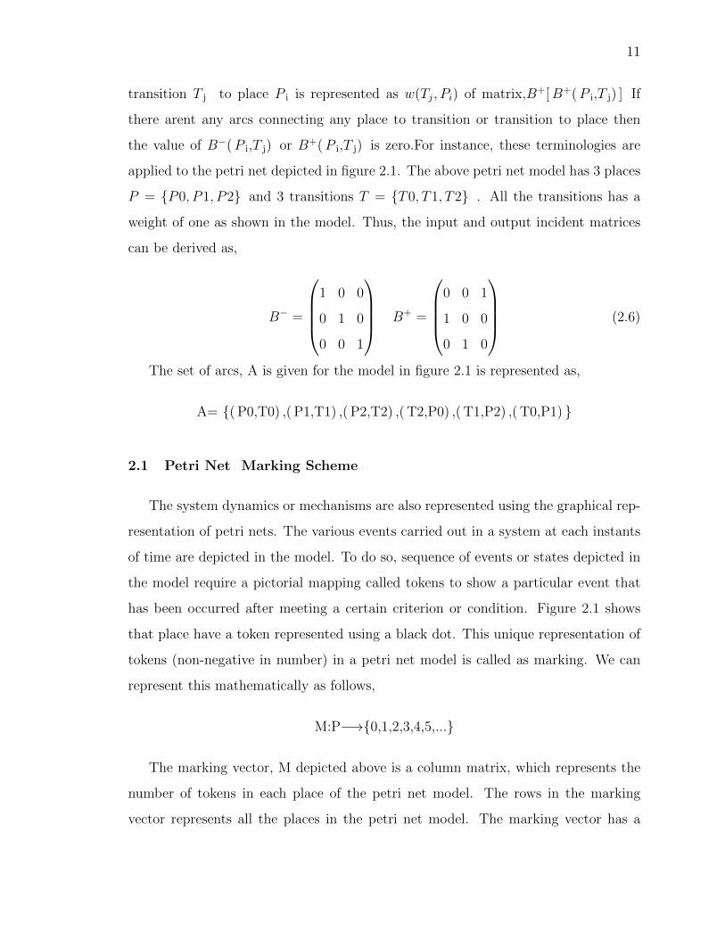
applied to the petri net depicted in figure 2.1. The above petri net model has 3 places
P = {P0, P1, P2} and 3 transitions T = {T0, T1, T2} . All the transitions has a
weight of one as shown in the model. Thus, the input and output incident matrices
can be derived as,
B− =
1 0 0
0 1 0
0 0 1
B+ =
0 0 1
1 0 0
0 1 0
(2.6)
The set of arcs, A is given for the model in figure 2.1 is represented as,
A= {( P0,T0) ,( P1,T1) ,( P2,T2) ,( T2,P0) ,( T1,P2) ,( T0,P1) }
2.1 Petri Net Marking Scheme
The system dynamics or mechanisms are also represented using the graphical rep-
resentation of petri nets. The various events carried out in a system at each instants
of time are depicted in the model. To do so, sequence of events or states depicted in
the model require a pictorial mapping called tokens to show a particular event that
has been occurred after meeting a certain criterion or condition. Figure 2.1 shows
that place have a token represented using a black dot. This unique representation of
tokens (non-negative in number) in a petri net model is called as marking. We can
represent this mathematically as follows,
M:P−→{0,1,2,3,4,5,...}
The marking vector, M depicted above is a column matrix, which represents the
number of tokens in each place of the petri net model. The rows in the marking
vector represents all the places in the petri net model. The marking vector has a

12
value zero if a particular places does not have any tokens. M(Pi) describes marking
vector of a place ( i.e., total number of tokens in place, Pi) where i represent the
place denoted in the model. For instance, if we consider the example model shown in
figure 2.2, M( P0) = 1, M( P1) = 0, M( P2) =0 and it can be seen that places P2 and
P1 has no tokens hence the value corresponding to it in the marking vector is zero.
Thus, number of tokens and corresponding value in the marking vector is always any
positive integer greater than or equal to zero. M0 denotes the initial marking vector
of a petri model, i.e., state of the system before any transition or event is about to
occur or get triggered. M1, M2 and so on are the next successive marking vectors
that represent the state of the system after successive transitions have been triggered.
Fig. 2.2. Petri Net model- An Example
Considering the example in figure 2.2, the initial marking vector for the system is
as shown below,
M0 =
1
0
0
=(
1 0 0)T
(2.7)
Therefore, the marked Petri net (MPN) is given by the equation,
MPN = {P, T,A,w,M0} (2.8)
13
where M0 is the column vector representing the initial marked state of the model or
system i.e., marking of all places in the net and P, T,A and w are same as explained
above.
2.2 Petri Nets Dynamics
Once all parameters, including the placement of tokens, incident matrices of the
Petri net, etc., have been identified or defined, we can explain about the dynamics
of the Petri net which is nothing but the changing state of the model, i.e., change in
markings, due to the triggered transitions. When the number of tokens contained in
the input places is greater than or equal to the arc weight, we can say that a transition
is enabled. In other words, transition Tj is enabled for a particular marking Mk if
and only if the below condition is satisfied.
Mk(P i) ≥ B−(Pi, T j) (2.9)
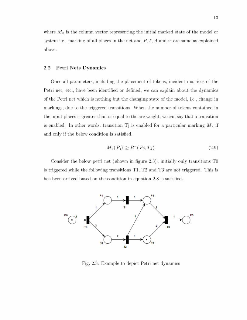
Consider the below petri net ( shown in figure 2.3) , initially only transitions T0
is triggered while the following transitions T1, T2 and T3 are not triggered. This is
has been arrived based on the condition in equation 2.8 is satisfied.
Fig. 2.3. Example to depict Petri net dynamics
14
Enabled transition and fireable transition are two different aspects generally, the
inequality equation above defines the condition for enabling a transition. Whereas,
the condition for firing is more general, i.e., to make a transition fireable it has to
be both enabled and satisfy other external conditions/events or a time condition.
For autonomous discrete Petri nets, those Petri nets which their dynamics are not
affected by external events not time, as soon as a transition gets enabled, it fires.
The dynamics of firing occurs in two steps, but it is an immediate process assumed
to not have any time duration. First, a specific number of tokens are moved to the
transitions from each input place to that transition. The number of tokens moved is
equal to the weight of the arc that connects the input place to the transition. Second,
tokens are transferred from the transition to all its output places. The number of
tokens transferred to each output place is equal to the weight of the arc connecting
the transition to the destination place [12].
To get a broader picture about the same let us consider our previous example from
figure 2.3. Transitions T0 is triggered while the following transitions T1,T2 and T3,
are not triggered. So T0 fires and a token is removed from place, P0 and then a token
is added to place P1 and 2 tokens are added to place, P2 respectively. Therefore,
initial marking M0=(
1 0 0 0 1 0)T
is changed to M1=(
0 1 2 0 1 0)T
following the transition,T0 This process of firing can be expressed as, M1 t0−→ M1.
Now, after the firing of transition, T0, the following transitions, T1, T2 are
enabled. So there are 2 case, case 1: T1 gets triggered first and then transition
T2 and case 2: first T2 gets triggered and then T1 gets triggered. Considering
the case 1, firing T1 from the marking M1=(
0 1 2 0 1 0)T
so we get M2=(0 0 2 1 1 0
)Tand no additional transitions are triggered. Now, triggering T2
then M3=(
0 0 0 02 2 0)T
. Following the above transition T2, transition T3,
gets triggered and 2 tokens each from places P3 and is removed and placed in P5 and
marking the terminal node with marking M5=(
0 0 0 0 0 1)T
. Now let us con-
sider the case 2, so firing transition T2 from the marking M1 =(
0 1 2 0 1 0)T
15
so we get M2 =(
0 1 0 1 2 0)T
and no additional transitions are triggered.
Then, triggering T1 so, M3=(
0 0 0 2 2 0)T
. Following, the above transition
T1, T3 gets triggered and 2 tokens each from places P3 and P4 is removed and
added in P5 and marking the terminal node with marking M5=(
0 0 0 0 0 1)T
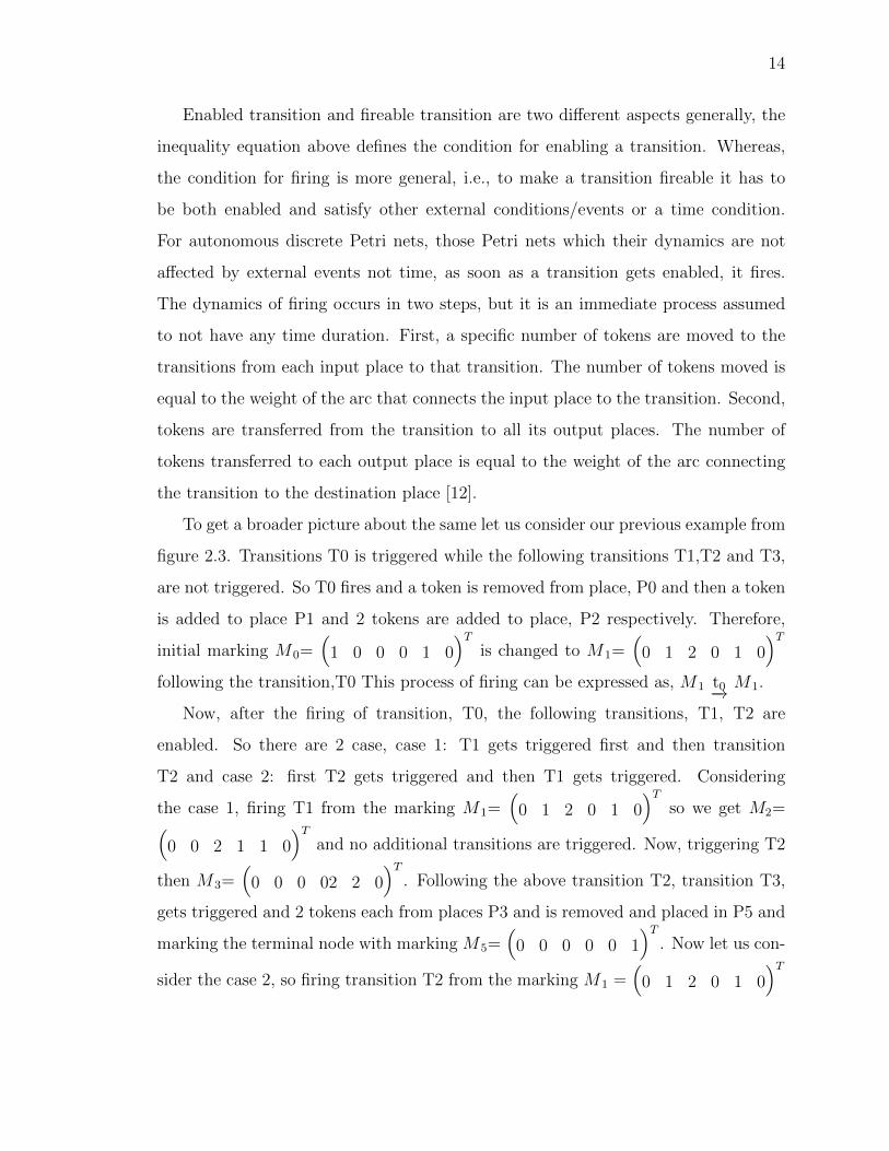
Therefore, to provide an easier analysis of Petri nets dynamics, a chart showing all
the column vectors of all possible marking connected through transitions (arcs) called
reachability graph comes into picture. The reachability graph provides us with all
possible markings and its generated sequence of the model from figure 2.3, is as shown
in figure 2.4 below.
Fig. 2.4. Reachability Tree for Petri Net model
Sometimes, in certain models of Petri Nets, the total reachable states or markings
can be infinite. That is at-times a place can have an unbounded number of tokens are

16
hence called as unbounded Petri Net models and becomes less possible to analyze all
reachable states of the model using a reachability graph. In such cases, a converabilty
root tree technique is utilized to describe the states, this has been explained in more
depth by David and Alla [?].
2.3 Petri Nets State Equation
Considering the previous example for Petri net in figure 2.3, it was to derive all
possible reachable states and study about the firing sequences. However, this becomes
overwhelming as number of places in the model increases and then the marking grows
exponentially, this makes it extremely difficult and at times nearly impossible to
analyze larger and complicated systems. As we know, the bipartite model of Petri
nets provides a mathematical equation in linear algebra and by solving it via program
simplifies the generation of final marking state from its initial marking through a
sequence of triggered transitions. As defined above, the marked petri net is defined
as MPN = {P, T,A,w,M0} and the matrices B− and B+ have a dimension of N× M
Where N denotes the number of places and M denotes the number of transitions in
the Petri net model.
17
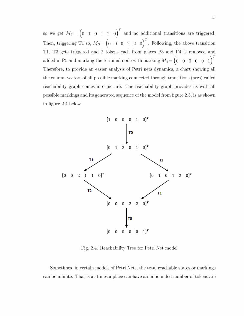
Now, introducing the matrix B of N× M dimension, which is defined as matrix
formed from the difference of output incident matrix and input incident matrix and
is called the incident matrix. The incident matrix of the example in the figure 2.3 is
explained below,
B = B+ −B−
=
0 0 0 0
1 0 0 0
2 0 0 0
0 1 1 0
0 0 1 0
0 0 0 1
−
1 0 0 0
0 1 0 0
0 0 2 0
0 0 0 2
0 0 0 2
0 0 0 0
=
−1 0 0 0
1 −1 0 0
2 0 −2 0
0 1 1 −2
0 0 1 −2
0 0 0 1
(2.10)
Now, the algebraic or the state equation of Petri net is defined as,
M ′k+1 = Mk +B.S (2.11)
WhereMk is the marking column vector ( N×1) of Petri net before the firing sequence
S ( M× 1) andM ′k+1 is the marking column vector ( N×1) after the transition defined
by firing sequence S ( M ×1) has been occurred, Mk s−→ M ′k+1.Considering example
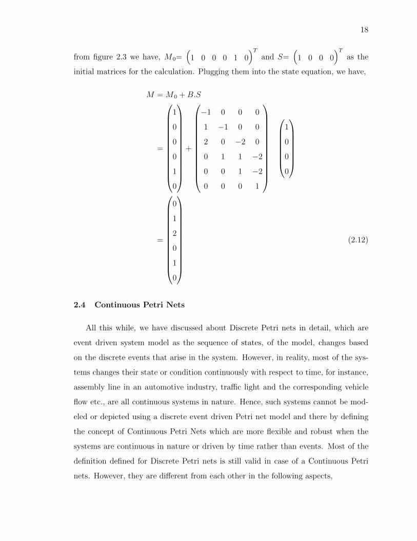
18
from figure 2.3 we have, M0=(
1 0 0 0 1 0)T
and S=(
1 0 0 0)T
as the
initial matrices for the calculation. Plugging them into the state equation, we have,
M = M0 +B.S
=
1
0
0
0
1
0
+
−1 0 0 0
1 −1 0 0
2 0 −2 0
0 1 1 −2
0 0 1 −2
0 0 0 1
1
0
0
0
=
0
1
2
0
1
0
(2.12)
2.4 Continuous Petri Nets
All this while, we have discussed about Discrete Petri nets in detail, which are
event driven system model as the sequence of states, of the model, changes based
on the discrete events that arise in the system. However, in reality, most of the sys-
tems changes their state or condition continuously with respect to time, for instance,
assembly line in an automotive industry, traffic light and the corresponding vehicle
flow etc., are all continuous systems in nature. Hence, such systems cannot be mod-
eled or depicted using a discrete event driven Petri net model and there by defining
the concept of Continuous Petri Nets which are more flexible and robust when the
systems are continuous in nature or driven by time rather than events. Most of the
definition defined for Discrete Petri nets is still valid in case of a Continuous Petri
nets. However, they are different from each other in the following aspects,
19
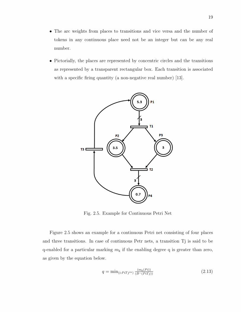
• The arc weights from places to transitions and vice versa and the number of
tokens in any continuous place need not be an integer but can be any real
number.
• Pictorially, the places are represented by concentric circles and the transitions
as represented by a transparent rectangular box. Each transition is associated
with a specific firing quantity (a non-negative real number) [13].
Fig. 2.5. Example for Continuous Petri Net
Figure 2.5 shows an example for a continuous Petri net consisting of four places
and three transitions. In case of continuous Petr nets, a transition Tj is said to be
q-enabled for a particular marking mk if the enabling degree q is greater than zero,
as given by the equation below.
q = min(i:PiTjin)(mk(Pi))
(B−(PiTj))(2.13)

20
This means that the enabling degree q of the transition Tj at the marking mk is
the minimum value of division each marking of the transition Tj input places on the
weight of the arc connects that place to the transition. Note that q is a finite positive
real number.
From figure 2.5, after applying the enabling degree definition, we have, transition
T1 is 3-enabled, transition T2 is 2-enabled and the transition T3 is 0.7-enabled.
However, the mechanisms behind a continuous Petri net is different from that of a
discrete Petri Net in terms of enabling conditions. To further understand the firing
of a transition and the corresponding firing sequence of continuous Petri Nets, a new
notation is introduced: α. A transition Tj is fired by the value α at one time is
represented as [Tj] α. For instance, [T3] 0.4 means that transition T3 is fired by the
amount of 0.4, that is 0.4 tokens are removed from the continuous place, P4 and are
added to continuous place, P1. The marking for the model is therefore modified to:
s =(
5.7 3.5 3 0.3)T
from s =(
5.3 3.5 3 0.7)T
Now, for continuous Petri nets, the total number of possible reachable states are
often infinite even when it is bounded Petri nets. So, it becomes nearly impossible to
define all the reachable states in the reachability graph. Hence, we define a general
marking concept called macro marking to consider all the markings in the reachability
graph showing if the places have tokens or not. For instance, consider the petri net
from figure 2.5, having 4 places so it could have maximum of 16 macro markings.
That is a Petri net model with n places has 2n macro-markings possible. 16 macro-
markings:(0 0 0 0
)T (m1 0 0 0
)T (0 m2 0 0
)T (0 0 m3 0
)T(
0 0 0 m4
)T (m1 m2 0 0
)T (m1 0 m3 0
)T (m1 0 0 m4
)T(
0 m2 m3 0)T (
0 m2 0 m4
)T (0 0 m3 m4
)T (m1 m2 m3 0
)T(m1 0 m3 m4
)T (m1 m2 0 m4
)T (0 m2 m3 m4
)T (m1 m2 m3 m4
)T
21
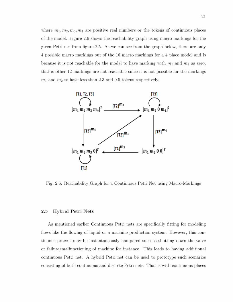
where m1,m2,m3,m4 are positive real numbers or the tokens of continuous places
of the model. Figure 2.6 shows the reachability graph using macro-markings for the
given Petri net from figure 2.5. As we can see from the graph below, there are only
4 possible macro markings out of the 16 macro markings for a 4 place model and is
because it is not reachable for the model to have marking with m1 and m2 as zero,
that is other 12 markings are not reachable since it is not possible for the markings
m1 and m2 to have less than 2.3 and 0.5 tokens respectively.
Fig. 2.6. Reachability Graph for a Continuous Petri Net using Macro-Markings
2.5 Hybrid Petri Nets
As mentioned earlier Continuous Petri nets are specifically fitting for modeling
flows like the flowing of liquid or a machine production system. However, this con-
tinuous process may be instantaneously hampered such as shutting down the valve
or failure/malfunctioning of machine for instance. This leads to having additional
continuous Petri net. A hybrid Petri net can be used to prototype such scenarios
consisting of both continuous and discrete Petri nets. That is with continuous places

22
(represented as C - places) and continuous transitions (represented as C - transitions)
and discrete places (depicted as D - places) and discrete transitions (depicted as D -
transitions). In addendum, a discrete marking could be transformed into a continuous
marking and inversely a continuous marking to a discrete marking. The continuous
place markings are depicted by using a real number, called a mark, and dots consti-
tute to be the marking for a discrete place, called tokens. Marked hybrid Petri nets
consist of six basic components:
HPN = {P, T,B−, B+,m0, hPN} (2.14)
Where, hPN represents the hybrid function to depict the places and transitions for a
continuous or a discrete Petri net model.
hPN : P ∪ T −→ {C,D} (2.15)
As mentioned earlier in the discrete Petri net model, {P, T,B−, B+,m0, hPN} holds
the same descriptions. But here, P contains both discrete and continuous places
similarly T contains all the transitions both continuous and discrete. Say, PC depicts
set of all continuous places and PD depicts set of all discrete places for any hybrid
Petri net model HPN then, P= PC ∪ PD. Likewise, if TC depicts set of all possible
continuous transitions and TD depicts set of all possible discrete transitions for the
HPN model then, T= TC ∪ TD. Also, here m0 represent the initial marking for the
hybrid Petri net model with markings of both continuous and discrete places. Say,
MD equals set of all markings of all discrete places of the HPN model and MC equals
set of all markings of all continuous places of the HPN model. Also, say mc and md
represents the number of continuous and discrete places respectively. Then,
M0 = (Mc,MD)
= [P0, P1, ..Pmc−1PmcPmc+1....Pmc+md−2Pmc+md−1
] (2.16)
Additionally, the arcs joining a discrete place to a continuous transition should
be equal in their arc weights. That is for, Pc, describing a continuous place Pd,

23
describing a discrete place tc, describing a continuous transition and Td, describing a
discrete transition, related using the below equation has to be satisfied for all possible
places and transitions of the particular HPN model.
B+( Pd, Tc) = B−( Pd, Tc) (2.17)
Also, the hybrid Petri model have different rules for enabling conditions due to
the presence of continuous and discrete places and transitions within the model.
Case 1: Discrete transitions the same rule mentioned for discrete Petri net models
are still valid. It is not applicable if a place is discrete or continuous. So, a discrete
transition TDj is enabled for a particular marking Mk if the below condition is satisfied
irrespective of the nature of the places.
Mk(Pi) ≥ B−(Pi, TDj ) (2.18)
Case 2: Continuous transitions: A continuous transition TCj is enabled for a
particular marking Mk if and only if the below condition(s) are satisfied.
Continuous transition TjC and for every input places that are discrete:
Mk(PiD) ≥ B−(PiD, T jC) (2.19)
Continuous transition TCj and for every input places that are continuous:
Mk(Pic) ≥ 0 (2.20)
The state equation for hybrid Petri net HPN is given by the relation same as
the one for discrete model but here we just need to include the continuous markings
too and the components can be an integer or a real number based on discrete or
continuous transitions respectively.
M ′k+1 = Mk +B.S (2.21)
Consider the hybrid Petri net shown in figure 2.7. Here, P0 and P1 are discrete
places and P2, P3 and P4 are continuous places of the hybrid model. Also, TD1 and
TC2 are discrete and continuous transitions respectively.

24
Fig. 2.7. Example for Hybrid Petri Net Model
The initial marking is M0=(MD,MC) equals, M0=(
1 0 6.4 4.2 3)T
. Now
here only transition TD1 is enabled and the new marking is M1=(
0 1 6.4 4.2 3)T
and now the transition TC2 is enabled until all the tokens from P3 is transferred to
P4 and the new marking for α = 0.4([TC2 ]0.4) is M2=(
0 1 6 4.2 3)T
. And the
final marking for the given hybrid model when none of the transitions are enabled
is M12=(
0 1 2 0.2 7)T
David and Alla have more examples [10, 11] that gives
more insight regarding state equations and various changes associated with state of
hybrid Petri nets [14].

25
3. ADAPTIVE CRUISE CONTROL SYSTEM
IMPLEMENTATION
3.1 Definition
Adaptive cruise control is a basic part of ADAS systems. It is an add-on intel-
ligence to the present cruise control system. It is also called as Autonomous cruise
control, Predictive cruise control or Radar cruise system. The vehicle is equipped
with a radar system under the bumper which detects when there is a car in the same
lane and the desired speed is set by the driver as usual with cruise control. Once the
car is detected, the distance between the cars can be adjusted accordingly to maintain
a safe distance as shown in figure 3.1. Sensors play a key role in ACC and almost
all ADAS systems. Here, instead of RADAR we can use LiDAR, infrared cameras
according to the necessity.
Fig. 3.1. ACC Concept
26
The adaptive cruise controls systems that are currently used in the vehicles use on-
board sensors like a stereo camera or radar or laser, which help in detecting the vehicle
ahead based on their sensing capabilities. According to the levels of automation
specified by the SAE, vehicles equipped only with adaptive cruise control are classified
as level 1 [15].
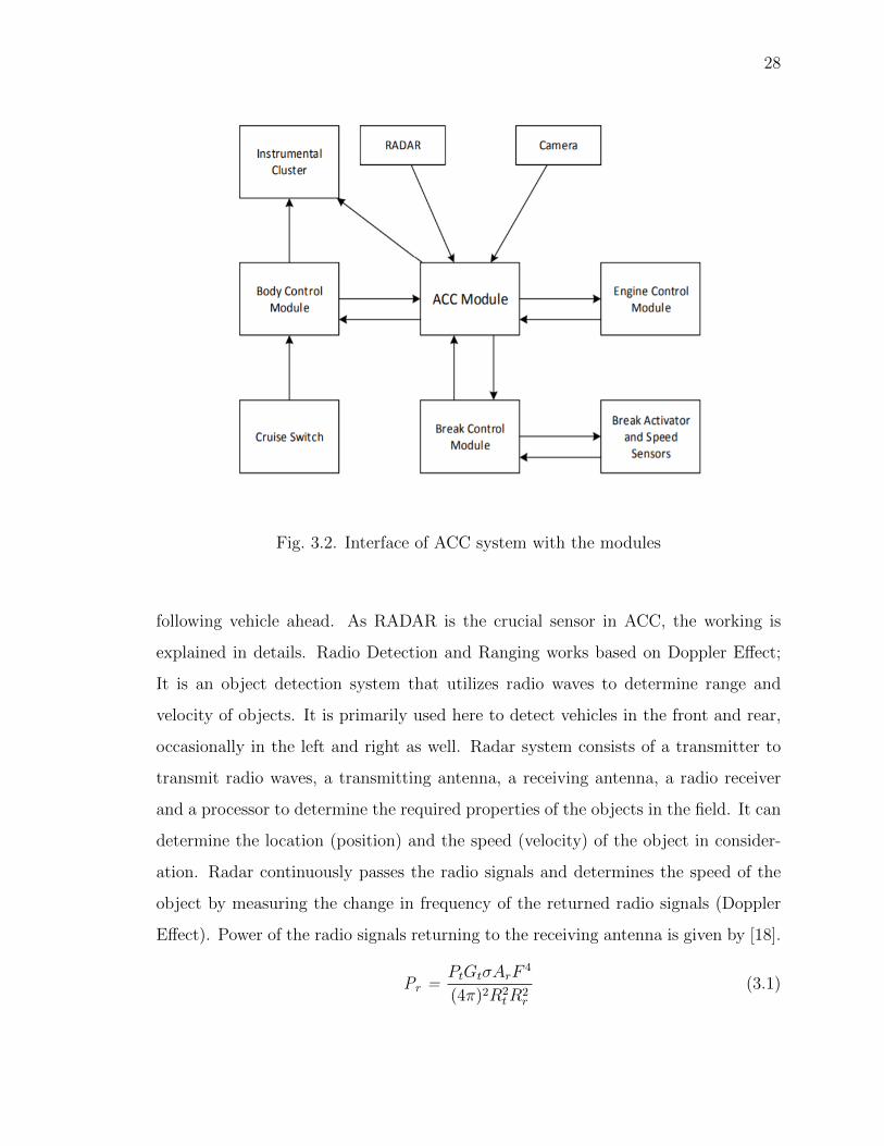
3.2 Adaptive Cruise Control system interface
The model of ACC can be divided into upper-level model and lower-level model.
UL model consists of acceleration as input and position of vehicle as output. Lower
level model has accelerator or brake as input and vehicle’s acceleration as output [16].
UL model represents the distance between the two car. It is basically calculated by
using the Constant Time-Gap (CTG). Since we are dealing with the moving vehicle
dynamics, Variable Time Gap (VTG) is considered [17]. So there are various com-
ponents involved to formulate an algorithm for the vehicle movement matching with
the front vehicle. The major ones are Control unit, sensors, and the communication
protocol as shown in figure 3.2.
3.2.1 Control Unit
• Adaptive Cruise Control Module: The main function of the Adaptive cruise
control modules is to process the information coming from the radar regarding
the target presence and identification of the correct target. If the ACC sys-
tem can consist of both the Radar and Camera sensors then the ACC module
processes and fuses the information from both the sensors for identifying the
correct target. It also has the responsibility of sending the corresponding infor-
mation to Engine control module, brake control module, and other modules for
maintaining the set distance of the ACC.
27
• Body Control Module: The main function in this process is to take the input
from the driver using the steering wheel switches or other switches used by
the ACC and sends the information to the ACC module and to the instrument
cluster to notify the driver of his input. The BCM uses communication protocol
like Local Interconnect network (LIN) to communicate with the switches.
• Engine Control Module: The main function of the engine control module is to
receive the speed commanded by the ACC feature and then adjust the engine
throttle accordingly to change the vehicle speed. Engine control module in turn
communicates with other modules like Transmission control module to change
the commanded gear for increasing or decreasing speeds.
• Brake Control Module: If ACC is commanding a decrease in speed then it
sends the information to the brake control module which gets the vehicle speeds
from the wheel speed sensors in each wheel to decrease the speed accordingly
using braking systems like Antilock Braking system (ABS) which is a hydraulic
braking system with electronic enhancement.
• Instrument Cluster: Instrument cluster receives information from the ACC
module to notify the driver about the status of the ACC Feature. The Current
status includes information on, graphics indicating presence of a target vehicle,
Driver information center text messages when ACC enabled and disabled, ACC
Gap setting information commanded by the driver using the steering wheel
controls, informations indicating the current set speed of the ACC, etc.
3.2.2 Sensors
The ACC feature implemented using multiple sensors, like using both radars and
camera to increase the detection efficiency and reliability to detect the traffic upfront.
These type of ACC systems are accompanied by other driver assist features like the
lane assist and lane maintaining system to help the car be in the same lane while
28
Fig. 3.2. Interface of ACC system with the modules
following vehicle ahead. As RADAR is the crucial sensor in ACC, the working is
explained in details. Radio Detection and Ranging works based on Doppler Effect;
It is an object detection system that utilizes radio waves to determine range and
velocity of objects. It is primarily used here to detect vehicles in the front and rear,
occasionally in the left and right as well. Radar system consists of a transmitter to
transmit radio waves, a transmitting antenna, a receiving antenna, a radio receiver
and a processor to determine the required properties of the objects in the field. It can
determine the location (position) and the speed (velocity) of the object in consider-
ation. Radar continuously passes the radio signals and determines the speed of the
object by measuring the change in frequency of the returned radio signals (Doppler
Effect). Power of the radio signals returning to the receiving antenna is given by [18].
Pr =PtGtσArF
4
(4π)2R2tR
2r
(3.1)
29
where,
Pr - Power of the transmitter
Pt - Power of the receiver
Gt - Gain of the transmitting antenna
Ar - effective aperture (area) of the receiving antenna where, Ar=Grλ4π
Gr - Gain of the receiving antenna
λ Transmitted length
σ - Radar cross section F - Pattern propagation factor Rt - distance between
transmitter to target (object) Rr distance from target (object) to receiver
ACC uses active radar, in that, radio signals are transmitted and reflected back.
The Doppler frequency is given by [19],
FD = 2× FT ×VRC
(3.2)
where,
FD - Doppler frequency
FT - transmit frequency
C - speed of light 3 × 10⁸ (m/s)
VR - radial velocity
Radar currently used in ACC is when the ACC is switched ON, Radar starts
detecting objects (say greater than 25 mph) and if there is a vehicle, say at 1 or 2
vehicle distance in the front or rear, it alerts the user and accelerates/decelerates the
vehicle based on the requirement. For example, if the vehicle in the front is cruising
at 60 mph and the user is cruising at 70 mph, the Radar detects the distance and
reduces the user speed to 60 mph. But assuming there is a vehicle cruising at 65 mph
in the rear; our smart ACC system finds a balance between the two speeds (say 62.5
mph) and alerts the user [20].
30
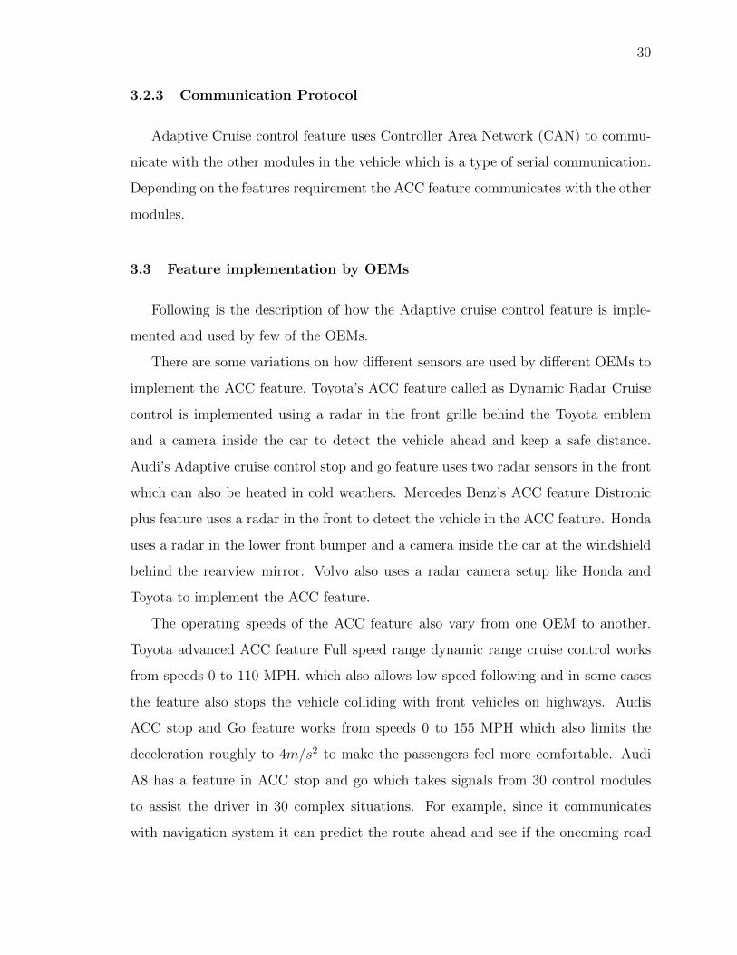
3.2.3 Communication Protocol
Adaptive Cruise control feature uses Controller Area Network (CAN) to commu-
nicate with the other modules in the vehicle which is a type of serial communication.
Depending on the features requirement the ACC feature communicates with the other
modules.
3.3 Feature implementation by OEMs
Following is the description of how the Adaptive cruise control feature is imple-
mented and used by few of the OEMs.
There are some variations on how different sensors are used by different OEMs to
implement the ACC feature, Toyota’s ACC feature called as Dynamic Radar Cruise
control is implemented using a radar in the front grille behind the Toyota emblem
and a camera inside the car to detect the vehicle ahead and keep a safe distance.
Audi’s Adaptive cruise control stop and go feature uses two radar sensors in the front
which can also be heated in cold weathers. Mercedes Benz’s ACC feature Distronic
plus feature uses a radar in the front to detect the vehicle in the ACC feature. Honda
uses a radar in the lower front bumper and a camera inside the car at the windshield
behind the rearview mirror. Volvo also uses a radar camera setup like Honda and
Toyota to implement the ACC feature.
The operating speeds of the ACC feature also vary from one OEM to another.
Toyota advanced ACC feature Full speed range dynamic range cruise control works
from speeds 0 to 110 MPH. which also allows low speed following and in some cases
the feature also stops the vehicle colliding with front vehicles on highways. Audis
ACC stop and Go feature works from speeds 0 to 155 MPH which also limits the
deceleration roughly to 4m/s2 to make the passengers feel more comfortable. Audi
A8 has a feature in ACC stop and go which takes signals from 30 control modules
to assist the driver in 30 complex situations. For example, since it communicates
with navigation system it can predict the route ahead and see if the oncoming road
31
has curved lanes or not to see if the car should slow down. The Distronic plus ACC
feature in Mercedes Benz and ACC feature in Volvo operate from speeds 0 to 125
MPH.
The Gap that is set in the ACC feature which to be maintained between the host
vehicle and the vehicle ahead is either measured in absolute distance or time. In
Mercedes Benz, the driver can choose a distance of 100, 200 or 300 meters depending
on his preference and traffic condition. In Honda, the following distance does not
depend on absolute distance on the time. It has short (1.1s), middle (1.5s) long
(2.1s), Extralong (2.8s) gap setting to follow vehicle. In Volvo, the driver can choose
how ACC should use the preset time interval based on the drive mode. If the drive
mode is Eco, then the ACC maintains long interval to the vehicle ahead. If the mode
is comfort, then ACC try to follow the set time interval as smoothly as possible. If the
Drive mode is set to Dynamic, then ACC focuses on following the set time interval
to the vehicle ahead more closely, which may mean even heavier acceleration and
braking in few cases.
3.4 Model of Adaptive cruise control in Discrete Petri net
The modeling in this thesis was done by considering the host vehicle as our interest.
The Discrete Petri net part of the model will be used to depict the high-level events
that happen in Autonomous cruise control system. The various versions of the model
are discussed in this section with the explanation of the drawbacks of each model and
how it was overcome in the following versions
3.4.1 Version 1
In working of a cars control system there are lot of factors to be considered from
key ON to Key OFF. Once Key-ON, engine gets fuel supply and the car moves.
The data from various sensors are communicated through to CAN, LIN. The process
behind the engine ON and the acceleration of the vehicle is out of scope for this

32
Fig. 3.3. Flow Chart of Version 1
research. Even there are many co-systems of ACC like ABS, Lane tracker, collision
avoidance, etc, that shares the sensors and can be integrated together for autonomous
vehicle development with car active safety. In this model 3.4, high-level events of the
adaptive cruise control system are captured and explained.
As per the control flow, once the car is ON, it is powering up the engine and the
other systems, in this case GPS tracker is being considered. As soon as the engine is
ON, the model checks for other power up such as Cruise control system and sensors
necessary for the ACC system to function. In this model 3.4, it is considered as we
33
have two RADAR system one in the front and other in the back. If there is a car
detected on either side, the radar system checks for the vehicle speed and distance
from both ends. There is an add on system which alerts user if the vehicle speed is
greater than current road speed limit. The speed limit data is extracted from the
GPS. Once the speed from the front and back vehicle is recorded, the values are
converged and the optimal speed for the vehicle is determined. The optimal speed
is converted by comparing the speed of the vehicles, by maintaining a constant set
distance on both sides. Then the calculated speed is send to the controller to change
the set speed. The control of events and control flow are shown in the Petri net model.
Model Explanation
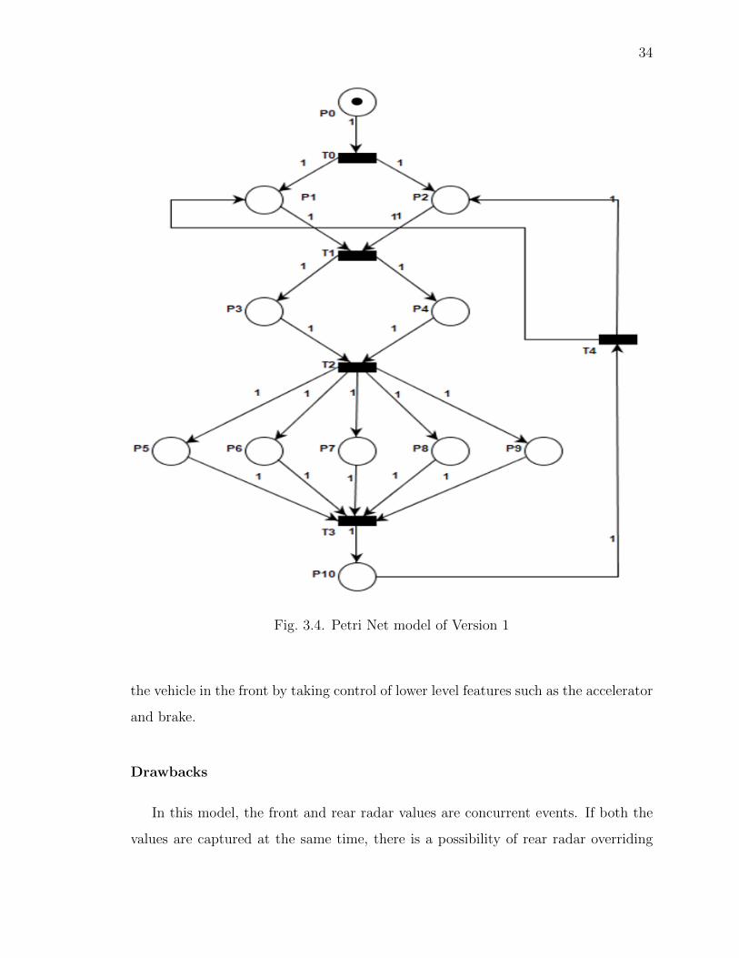
The working model of the autonomous cruise control system is explained in figure
3.4. Initially it is assumed that the car is ON so there is a token already existing
in place P0 and the weights on the arc is 1. A token in P0 triggers the transition
T0 which power ups the engine control module (ECM) and other system like GPS
in this case. When there are tokens in P1 and P2, it will trigger the transition T1,
which will pass the tokens to P3 and P4. Token in P3, P4 indicates the system check
for the enabling condition of the cruise control system and the sensors used by the
system (RADAR). These places again trigger the transition T2 to enable P5, P6, P7,
P8, P9, where P5 and P6 are the front Radar vehicle speed and distance respectively,
P8 and P9 are the rear radar vehicle speed and distance respectively and P9 is the
place for checking the speed limit for the current road and sending alert to the driver.
Once all the places have the token, the optimal speed for the situation is calculated
with the speed limit involved in the calculation and it will enable the transition T3
which sets the optimal speed. The set speed enables the transition T4 which acts as a
feedback loop from the set speed to the ECM. The transition T4 sends the calculated
set speed to the controller. This will adjust the speed of the vehicle with the speed of
34
Fig. 3.4. Petri Net model of Version 1
the vehicle in the front by taking control of lower level features such as the accelerator
and brake.
Drawbacks
In this model, the front and rear radar values are concurrent events. If both the
values are captured at the same time, there is a possibility of rear radar overriding
35
the front radar value if the calibration is not proper. In a case, when the front radar
stops detecting and we get a value from the rear radar which tends the speed of the
host vehicle without the concern about the front car. There is a high probability
of crash with the front car. Involving of rear radar is needless because we cannot
control the rear vehicles speed. If the rear vehicle speed is controlled, it opens the
scope to Vehicle to vehicle communication, a different area of research. So always for
this system, front radar should be given priority for calculating the speed of the host
vehicle at the fixed distance set by the driver.
3.4.2 Version 2
Considering, all the drawback from the old version, a new model is designed by
incorporating manual control option when the system fails. So in case when there is a
sensor failure, or cruise control system failure, the control shift to manual speed which
is set by the driver by accelerating or braking. Individual closed loop is designed for
both manual and ACC system.
The control flow is shown in the Figure 3.5. When the car is Key ON, the manual
control is activated i.e, the car is accelerating at a certain speed. When the driver
wants to activate the cruise control system, the CC button is ON. Once the cruise
control is activated, it checks for the system failure. If the system is not working,
the control goes to the manual driving. In this research system failure is considered
as cruise control system or RADAR failure. If the CC system is working, it checks
for the car in the front. Radar sensor plays a role in the car detection and finding
the distance between the cars. If there is no car in the front, the system takes the
set speed set by the Cruise control system. If there is a car in the front, it finds
the distance between the target car and the host car. With the desired distance the
speed of the target vehicle is observed that helps in calculating the optimal speed
of the host vehicle. Once we derive the optimal speed, the speed is achieved in the
host car by adjusting the throttle or brake of the car. When the driver accelerates
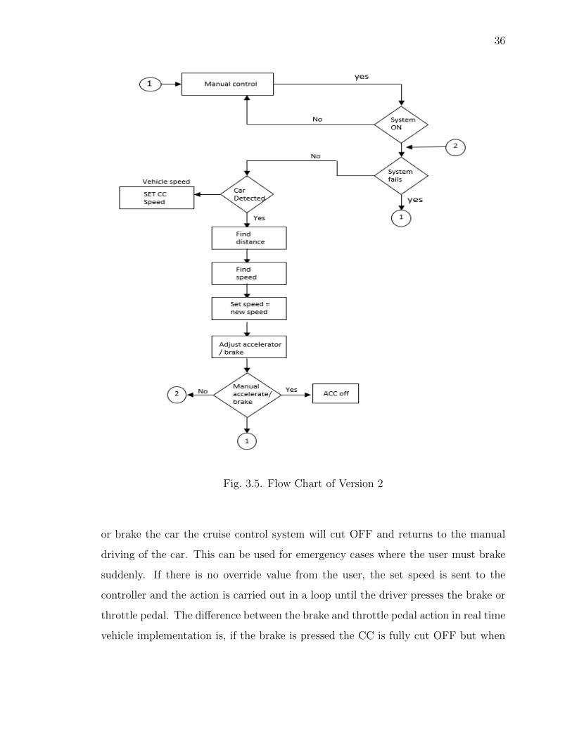
36
Fig. 3.5. Flow Chart of Version 2
or brake the car the cruise control system will cut OFF and returns to the manual
driving of the car. This can be used for emergency cases where the user must brake
suddenly. If there is no override value from the user, the set speed is sent to the
controller and the action is carried out in a loop until the driver presses the brake or
throttle pedal. The difference between the brake and throttle pedal action in real time
vehicle implementation is, if the brake is pressed the CC is fully cut OFF but when

37
the car is accelerated the controller takes the override value and once the throttle
pedal is released it comes back to the CC set speed unless the driver wants to brake
suddenly [21].
Fig. 3.6. Petri Net model of Version 2
The discrete Petri net model is shown for the updated version in Figure 3.6. As
an initial condition, there is a token in P1 assuming the car is ON. P1 activates the
38
transition T0, that transfers the token from P1 to P2. When there is a token in
P2, it states the car is in manual mode. Manual mode will trigger the transition T1
which transfers the token to P3 checking if the system is ON. If the system is ON the
T2 transition is triggered and the token is transferred to P4. The token in P4 can
trigger two transitions T3 and T5. The decision is made based on the CC systems
condition. If the system is failure, the transition P2. If the system is working it
will trigger T5 and starts to detect the front car if any when there is a token in P7.
Again, the transition T6, T7 will be triggered on decision basis when there is a token
in P7. The place P6 is for cruise control set speed. In the transition T8 the vehicle
distance is calculated, and a token is passed in place P8. The place P6, P8, P9, P10,
P11 are place for varying distances, speed of the front and host vehicle, current set
speed according to the target vehicle. P11 place is to check if the user is pressing
the accelerator or brake when CC is ON. If the user is accelerating or braking, the
transition T12 is carried out which is connected to the manual mode. If there is
no override value for the accelerator or brake position, a feedback loop is linked to
transition T2 and the process is carried it out in closed loop.
3.4.3 Drawbacks
There may be situations where the following distance can change drastically due to
the rapid change in speed of the target vehicle. To be more precise about the following
distance, ranges like critical, close range and safe range should be considered. The
control action of manual brake and accelerator should be considered two different
places since the outputs are different. Moreover, the cruise speed is not updated in
all situations. The case like cruise control switch OFF, when there is no vehicle in
the front, what if the system fails are not visualized in the model.

39
3.5 Final updated model
The final model is designed based on various analysis and considering drawbacks
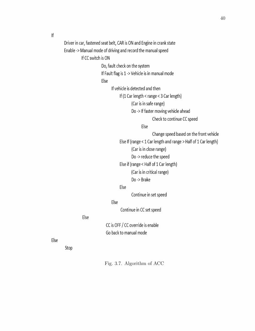
of all other models. A new algorithm is formulated considering all the cases involved
in the adaptive cruise control system. Similar to the algorithm stated below [22],
Set Timer to interrupt periodically in a period (T) at each interrupt
do,
1) Sensor Scan process (GPS, UI, Brake, Accel, Engine).
2) Get current speed.
3) Compute control values.
4) Update parameters.
5) Send adjustment value to throttle.
enddo
This algorithm states the events that happen for cruise control system. The
onboarding sensor values and the user’s set speed are the inputs. The step Compute
control values, will take car of the low level control and updates the parameter values
like accelration/deceleration values and the signal is set to the throttle for adjusting
the speed according to the set speed. For Adaptive cruise control, the higher level
events are captured and stated in the algorithm given in figure 3.7.
The various assumptions are the ACC is implemented in a manual driven car. The
autonomous or driverless cars are not in the scope of the research. Depending on the
OEMs, the minimum speed required to enable the cruise control differs. The fault
check flag basically checks the cruising system and the RADAR sensor. So, once the
Cruise button is ON by the driver, if the flag is 1, either there is no signal from the
cruise system or the RADAR signal is not sent to the ECU. In such case, the vehicle
will continue in the manual driving mode with the desired speed. Once, there is a
signal from both the system is received, the distance is calculated with respect to the
target vehicle. The distance can be categorized into 3 ranges as critical, close range
and safe range. The events and the control strategy is taken care for all the ranges. In
40
Fig. 3.7. Algorithm of ACC
41
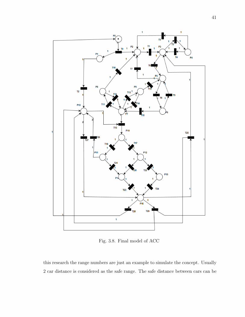
Fig. 3.8. Final model of ACC
this research the range numbers are just an example to simulate the concept. Usually
2 car distance is considered as the safe range. The safe distance between cars can be
42
defined according the target vehicle. There is a research on the safe distance [23] in
which they have explained the different way of calculating safe distance based on the
situation like braking process, based on headway, based on static target, slow moving
target [23] In this research the two conditions considered based on the target vehicle
are fast moving or slow moving vehicle. If the vehicle is moving fast, i.e, if the system
is too far from any target vehicle then it will begin to execute based on the cruise
control algorithm [24]. Basically it will try to match the velocity of the vehicle with
the set velocity. If the vehicle is slow, the cruise speed set value is adjusted internally
based on the velocity of the target vehicle (again velocity matching concept is carried
out.
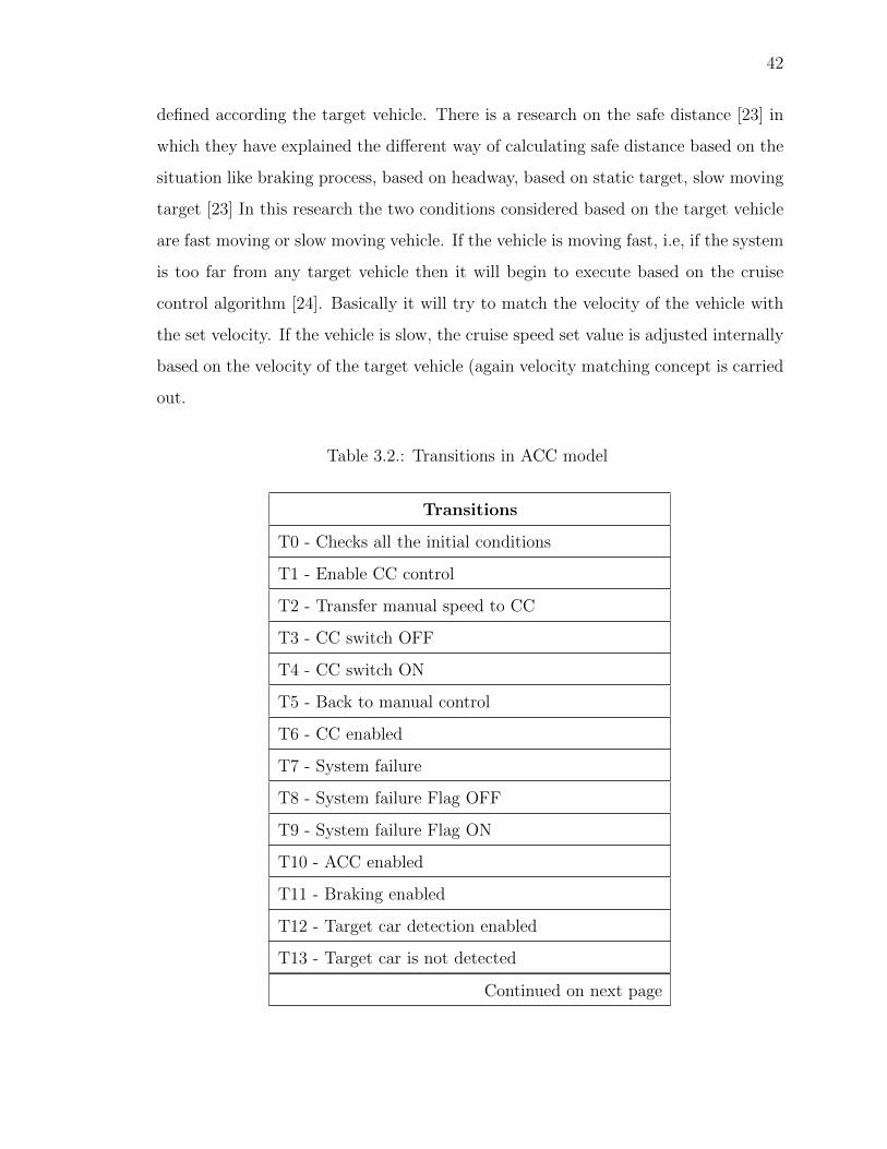
Table 3.2.: Transitions in ACC model
Transitions
T0 - Checks all the initial conditions
T1 - Enable CC control
T2 - Transfer manual speed to CC
T3 - CC switch OFF
T4 - CC switch ON
T5 - Back to manual control
T6 - CC enabled
T7 - System failure
T8 - System failure Flag OFF
T9 - System failure Flag ON
T10 - ACC enabled
T11 - Braking enabled
T12 - Target car detection enabled
T13 - Target car is not detected
Continued on next page
43
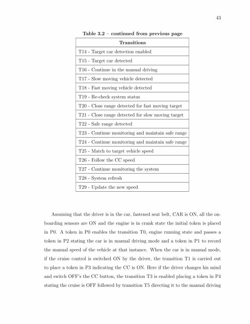
Table 3.2 – continued from previous page
Transitions
T14 - Target car detection enabled
T15 - Target car detected
T16 - Continue in the manual driving
T17 - Slow moving vehicle detected
T18 - Fast moving vehicle detected
T19 - Re-check system status
T20 - Close range detected for fast moving target
T21 - Close range detected for slow moving target
T22 - Safe range detected
T23 - Continue monitoring and maintain safe range
T24 - Continue monitoring and maintain safe range
T25 - Match to target vehicle speed
T26 - Follow the CC speed
T27 - Continue monitoring the system
T28 - System refresh
T29 - Update the new speed
Assuming that the driver is in the car, fastened seat belt, CAR is ON, all the on-
boarding sensors are ON and the engine is in crank state the initial token is placed
in P0. A token in P0 enables the transition T0, engine running state and passes a
token in P2 stating the car is in manual driving mode and a token in P1 to record
the manual speed of the vehicle at that instance. When the car is in manual mode,
if the cruise control is switched ON by the driver, the transition T1 is carried out
to place a token in P3 indicating the CC is ON. Here if the driver changes his mind
and switch OFF’s the CC button, the transition T3 is enabled placing a token in P4
stating the cruise is OFF followed by transition T5 directing it to the manual driving
44
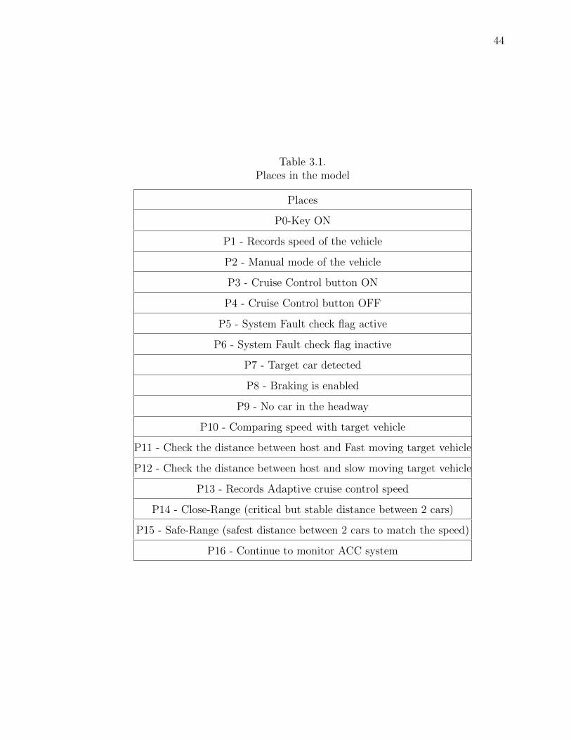
Table 3.1.Places in the model
Places
P0-Key ON
P1 - Records speed of the vehicle
P2 - Manual mode of the vehicle
P3 - Cruise Control button ON
P4 - Cruise Control button OFF
P5 - System Fault check flag active
P6 - System Fault check flag inactive
P7 - Target car detected
P8 - Braking is enabled
P9 - No car in the headway
P10 - Comparing speed with target vehicle
P11 - Check the distance between host and Fast moving target vehicle
P12 - Check the distance between host and slow moving target vehicle
P13 - Records Adaptive cruise control speed
P14 - Close-Range (critical but stable distance between 2 cars)
P15 - Safe-Range (safest distance between 2 cars to match the speed)
P16 - Continue to monitor ACC system
45
mode. The transition T6 enabled if the CC is in ON state which check the system
failure. In this transition, a Fault flag status is checked when there is a token in P5.
If there is a fault transition T7 is enabled to continue in the manual mode putting
a token in P2 or else T8 is fired placing token in P6 stating the system is working
enabling the transition T10. With T10 enabled a token is sent to P7 stating the car
is detected. When the car is detected, and it is in critical range, transition T11 is
carried out putting a token in P8 directing to P2 through transition T16.
If the ACC is enabled and there is no vehicle detected in the range, transition
T13 is carried out by putting a token in P9 directed to the system check by the
transition T19. To enable transition T15, a token from P7 and a token from P13 is
required. The place P13 gets enabled by the transition T2 noting the speed for the
CC control. It is a place that keeps updating the speed of the vehicle for all cases
basically considered as a buffer place. When there is token in P10 either T18 or T17
can fire. The decision is taken based on the target vehicle. If the target vehicle is
a fast moving vehicle T18 is fired else T17 is fired considering the target vehicle is
a slow moving one. Let’s consider the target vehicle is moving fast triggering T18
and a token in P11, now the distance range is noted. If the vehicle is in out of
range, T26 is fired and the vehicle follows in the set CC speed. If the range is a close
range where its not too close and not out of range, T21 is fired placing a token in
P14 which adjusts the velocity according to the target vehicle achieved by the low
level controls (accelerator or brake) in transition T23 and updated the current speed
in P13. Now, let’s consider the transition T17 from P10 which puts token in P12
indicating the slow moving vehicle ahead. Then if the distance is a close range, T20
else the cars are in safe range and transition T22 is carried out and putting a token
in P15. Transition T24 is similar to T23 placing a token in P16 which end up in
updating the speed in the place P13. The transition T25 is the one that compute
the values and update the adjusted speed in the place P13. For continue monitoring
purpose, enabling the transition T25 puts a token in P7 where it will check the fault
flag status and continues the working of the system.
46
The ACC can be in 4 states. ACC OFF, ACC active, ACC inactive and ACC
active and accelerate [24] The former 2 states are ON/OFF of ACC depending on the
vehicle detected. The manual action of driver can overrule the ACC state by pressing
the brake or accelerator. In cases when driver wants to increase the following distance
or planned to match the speed of the right lane if he intended to change lanes, the
driver presses the brake pedal and it goes to ACC inactive state enabling the transition
T28 to put token in the place P1 indicating the control of vehicle is done manually. In
case of decreasing the distance between the cars, overtaking the lead vehicle, the driver
decides to accelerates which puts the ACC in ”ACC active and accelerate” state. This
state will take the overridden acceleration as the current speed by disabling the set
speed for time-being and will be back to the set cruising speed once the driver releases
his/her leg from the throttle pedal. In this state, the transition T29 is enabled and
the current speed is updated in the place P13.
3.6 Invariant Analysis
According to the state equation stated in equation 2.10, the incident matrix, B of
the model is calculated using the input and output incident matrix B− and B+. The
matrices are as follows,
M0 =[1 0 0 0 0 0 0 0 0 0 0 0 0 0 0 0 0 0 0 0 0 0 0 0 0 0 0 0 0 0
](3.3)
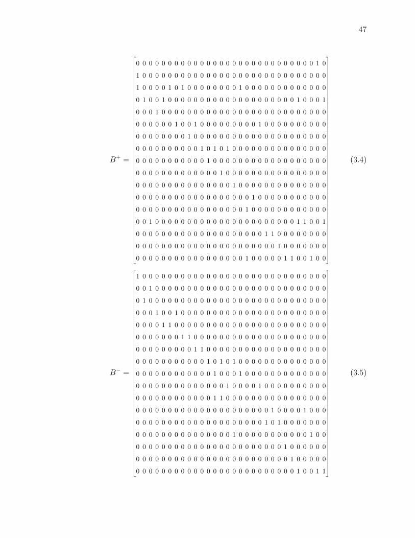
47
B+ =
0 0 0 0 0 0 0 0 0 0 0 0 0 0 0 0 0 0 0 0 0 0 0 0 0 0 0 0 1 0
1 0 0 0 0 0 0 0 0 0 0 0 0 0 0 0 0 0 0 0 0 0 0 0 0 0 0 0 0 0
1 0 0 0 0 1 0 1 0 0 0 0 0 0 0 0 1 0 0 0 0 0 0 0 0 0 0 0 0 0
0 1 0 0 1 0 0 0 0 0 0 0 0 0 0 0 0 0 0 0 0 0 0 0 0 1 0 0 0 1
0 0 0 1 0 0 0 0 0 0 0 0 0 0 0 0 0 0 0 0 0 0 0 0 0 0 0 0 0 0
0 0 0 0 0 0 1 0 0 1 0 0 0 0 0 0 0 0 0 1 0 0 0 0 0 0 0 0 0 0
0 0 0 0 0 0 0 0 1 0 0 0 0 0 0 0 0 0 0 0 0 0 0 0 0 0 0 0 0 0
0 0 0 0 0 0 0 0 0 0 1 0 1 0 1 0 0 0 0 0 0 0 0 0 0 0 0 0 0 0
0 0 0 0 0 0 0 0 0 0 0 1 0 0 0 0 0 0 0 0 0 0 0 0 0 0 0 0 0 0
0 0 0 0 0 0 0 0 0 0 0 0 0 1 0 0 0 0 0 0 0 0 0 0 0 0 0 0 0 0
0 0 0 0 0 0 0 0 0 0 0 0 0 0 0 1 0 0 0 0 0 0 0 0 0 0 0 0 0 0
0 0 0 0 0 0 0 0 0 0 0 0 0 0 0 0 0 0 1 0 0 0 0 0 0 0 0 0 0 0
0 0 0 0 0 0 0 0 0 0 0 0 0 0 0 0 0 1 0 0 0 0 0 0 0 0 0 0 0 0
0 0 1 0 0 0 0 0 0 0 0 0 0 0 0 0 0 0 0 0 0 0 0 0 0 1 1 0 0 1
0 0 0 0 0 0 0 0 0 0 0 0 0 0 0 0 0 0 0 0 1 1 0 0 0 0 0 0 0 0
0 0 0 0 0 0 0 0 0 0 0 0 0 0 0 0 0 0 0 0 0 0 1 0 0 0 0 0 0 0
0 0 0 0 0 0 0 0 0 0 0 0 0 0 0 0 0 1 0 0 0 0 0 1 1 0 0 1 0 0
(3.4)
B− =
1 0 0 0 0 0 0 0 0 0 0 0 0 0 0 0 0 0 0 0 0 0 0 0 0 0 0 0 0 0
0 0 1 0 0 0 0 0 0 0 0 0 0 0 0 0 0 0 0 0 0 0 0 0 0 0 0 0 0 0
0 1 0 0 0 0 0 0 0 0 0 0 0 0 0 0 0 0 0 0 0 0 0 0 0 0 0 0 0 0
0 0 0 1 0 0 1 0 0 0 0 0 0 0 0 0 0 0 0 0 0 0 0 0 0 0 0 0 0 0
0 0 0 0 1 1 0 0 0 0 0 0 0 0 0 0 0 0 0 0 0 0 0 0 0 0 0 0 0 0
0 0 0 0 0 0 0 1 1 0 0 0 0 0 0 0 0 0 0 0 0 0 0 0 0 0 0 0 0 0
0 0 0 0 0 0 0 0 0 1 1 0 0 0 0 0 0 0 0 0 0 0 0 0 0 0 0 0 0 0
0 0 0 0 0 0 0 0 0 0 0 1 0 1 0 1 0 0 0 0 0 0 0 0 0 0 0 0 0 0
0 0 0 0 0 0 0 0 0 0 0 0 1 0 0 0 1 0 0 0 0 0 0 0 0 0 0 0 0 0
0 0 0 0 0 0 0 0 0 0 0 0 0 0 1 0 0 0 0 1 0 0 0 0 0 0 0 0 0 0
0 0 0 0 0 0 0 0 0 0 0 0 1 1 0 0 0 0 0 0 0 0 0 0 0 0 0 0 0 0
0 0 0 0 0 0 0 0 0 0 0 0 0 0 0 0 0 0 0 0 0 1 0 0 0 0 1 0 0 0
0 0 0 0 0 0 0 0 0 0 0 0 0 0 0 0 0 0 0 0 1 0 1 0 0 0 0 0 0 0
0 0 0 0 0 0 0 0 0 0 0 0 0 0 0 1 0 0 0 0 0 0 0 0 0 0 0 1 0 0
0 0 0 0 0 0 0 0 0 0 0 0 0 0 0 0 0 0 0 0 0 0 0 1 0 0 0 0 0 0
0 0 0 0 0 0 0 0 0 0 0 0 0 0 0 0 0 0 0 0 0 0 0 0 1 0 0 0 0 0
0 0 0 0 0 0 0 0 0 0 0 0 0 0 0 0 0 0 0 0 0 0 0 0 0 1 0 0 1 1
(3.5)
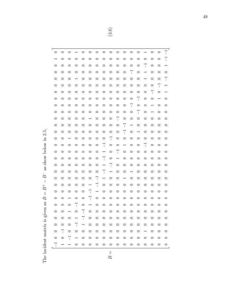
48
The
inci
den
tm
atri
xis
give
nasB
=B
+−B−
assh
owb
elow
in2.
5,
B=
−1
00
00
00
00
00
00
00
00
00
00
00
00
00
01
0
10−1
00
00
00
00
00
00
00
00
00
00
00
00
00
0
1−1
00
01
01
00
00
00
00
10
00
00
00
00
00
00
01
0−1
10−1
00
00
00
00
00
00
00
00
00
10
00
1
00
01−1−1
00
00
00
00
00
00
00
00
00
00
00
00
00
00
00
1−1−1
10
00
00
00
00
10
00
00
00
00
0
00
00
00
00
1−1−1
00
00
00
00
00
00
00
00
00
0
00
00
00
00
00
1−1
1−1
1−1
00
00
00
00
00
00
00
00
00
00
00
00
01−1
00
0−1
00
00
00
00
00
00
0
00
00
00
00
00
00
01−1
00
00−1
00
00
00
00
00
00
00
00
00
00
10
00
01
0−1−1
00
00
00
00
00
0
00
00
00
00
00
01
00
00
00
10
0−1
00
00−1
00
0
00
00
00
00
00
00
00
00
01
00−1
0−1
00
00
00
0
00
10
00
00
00
00
00
0−1
00
00
00
00
01
1−1
01
00
00
00
00
00
00
00
00
00
00
11
0−1
00
00
00
00
00
00
00
00
00
00
00
00
00
00
10−1
00
00
0
00
00
00
00
00
00
00
00
00
00
00
01
1−1
01−1−1
(3.6
)
49
3.6.1 Place invariant
The place invariant is given by sets of places whose number of token weights
remains constant for all possible markings. It can be explained as,
x1.M(P0) + x2.M(P1) + ....+ xk.M(Pk) = x0 (3.7)
where x0 is the constant. The place invariant of the model is given as,
2M(P0) +M(P1) +M(P2) +M(P3) +M(P4) +M(P5) +M(P6) +M(P7)
+M(P8) +M(P9) + 2M(P10) + 2M(P11) + 2M(P12) +M(P13)
+ 2M(P14) + 2M(P15) + 2M(P16) = 2 (3.8)
In the developed Petri net model of ACC, all the places with the weights on the
arc form the place invariant with the co-efficient 2. For instance, considering the
initial condition, M(P0)= 1, and all other markings(M(P1) + M(P2) + ... + M(P16)
are 0. Substituting in the equation 3.8, we get,
2× 1 + 0 + 0 + ...+ 0 = 2 (3.9)
Thus satisfying the place invariant condition.
3.6.2 Transition Invariant:
The model is bounded and following are the various transition invariants,
T3 + T4: Turning ON and OFF cruise control system doesnt increment number
of state of CC system of being from ON/OFF. That is the state remains in either
ON/OFF for any number of transitions (triggering T3, T4).
T1 + T3 + T5: Once the CC system is OFF, the number of tokens involved being
in the state of Manual Control CC System OFF, remains same.
T1+T6+T7: Once the CC system is ON and System adheres a failure, the number
of tokens involved during the loop for any number of transitions (triggering T1, T6, T7)
in any fashion remains the same.
50
T8 + T9: RADAR System Failure and Active doesn’t change the number of state
of RADAR system of being from Failure/Active. That is the state remains in either
Failure/Active for any number of transitions (triggering T8, T9).
T11 + T12: Triggering Breaking to Manual mode or Target Car detection for any
number of times doesnt change the tokens involved in the system of being from
breaking/target detected. That is the state remains in either breaking/target detected
for any number of transitions (triggering T11, T12).
T13 + T14 Triggering Target not detected or Target Car detected for any number
of times doesn’t change the tokens involved in the system of being from detected/not
detected. That is the state remains in either detected/not detected for any number
of transitions (triggering T13, T14).
T6 + T8 + T10 + T11 + T16: When a target car is detected and is too close to
the host car, where only possibility is to break, then the system remains in any of
the following state that is CC system is ON, RADAR system is Active, Target is
Detected and Breaking and transfer to Manual control mode and loop until new
states are found.
T8 + T10 + T13 + T19: When a target car is not detected, then the system remains
in any of the following state that is RADAR system is Active, Target is Check and
Target Not Detected and transfer back to RADAR system check and loop until new
states are found.
T0 +T1 +T2 +T6 +T8 +T10 +T15 +T17 +T20 +T23 +T28: When a manual breaking
is inquired while in ACC with Fast Target Vehicle and Safe Distance detection, then
system remains in any of the following state that is, Manual Control mode, CC system
ON, RADAR system Active, Target Vehicle Detected, Fast moving target detected,
a Safe distance between the 2 vehicles detected and Manual breaking detected. Then
loop back to Manual Control mode until new states are found.
T0+T1+T2+T6+T8+T10+T15+T17+T22+T24+T28: When a manual intervention
is inquired while in ACC with Fast Target Vehicle and Close Distance detection, then
system remains in any of the following state that is, Manual Control mode, CC system
51
ON, RADAR system Active, Target Vehicle Detected, Fast moving target detected, a
Close distance between the 2 vehicles detected and Manual breaking detected. Then
loop back to Manual Control mode until new states are found.
T0 +T1 +T2 +T6 +T8 +T10 +T15 +T18 +T26 +T27 +T28: When a manual breaking
is inquired while in ACC with Slow Target Vehicle and Cruise Mode, then system
remains in any of the following state that is, Manual Control mode, CC system ON,
RADAR system Active, Target Vehicle Detected, Slow moving target detected, a Safe
distance between the 2 vehicles detected so be in cruise mode, and Manual breaking
detected. Then loop back to Manual Control mode until new states are found.
T0+T1+T2+T6+T8+T10+T15+T18+T21+T23+T28: When a manual breaking is
inquired while in ACC with Slow Target Vehicle and Close Distance detection, then
system remains in any of the following state that is, Manual Control mode, CC system
ON, RADAR system Active, Target Vehicle Detected, Slow moving target detected, a
Close distance between the 2 vehicles detected and Manual breaking detected. Then
loop back to Manual Control mode until new states are found.
T6 +T8 +T10 +T15 +T17 +T21 +T23 +T25: When in ACC with Slow moving Target
Vehicle and Close Distance detection, then system remains in any of the following
state that is CC system is ON, RADAR system Active, Target Vehicle Detected,
Slow moving target detected, a Close distance between the 2 vehicles detected and
updating new CC speed. Then loop back to Cruise System status check until new
states are found.
T6 +T8 +T10 +T15 +T18 +T25 +T26 +T27: When in ACC with Slow moving Target
Vehicle enabling cruise mode, then system remains in any of the following state that
is CC system is ON, RADAR system Active, Target Vehicle Detected, Slow moving
target detected, a safe distance between the 2 vehicles detected enabling cruise mode
and updating new cruise speed. Then loop back to Cruise System status check until
new states are found.
T6 + T8 + T10 + T15 + T17 + T20 + T23 + T29: When a manual acceleration is
inquired while in ACC with Fast moving Target Vehicle at a close range, then system
52
remains in any of the following state that is CC system is ON, RADAR system Active,
Target Vehicle Detected, Slow moving target detected, a close distance between the
2 vehicles detected and new manual acceleration detected and updated. Then loop
back to Cruise System status check until new states are found.
T6 +T8 +T10 +T15 +T18 +T21 +T23 +T29: When a manual acceleration is inquired
while in ACC with Slow moving Target Vehicle at a close range, then system remains
in any of the following state that is CC system is ON, RADAR system Active, Target
Vehicle Detected, Slow moving target detected, a close distance between the 2 vehicles
detected and new manual acceleration detected and updated. Then loop back to
Cruise System status check until new states are found.
T6 +T8 +T10 +T15 +T17 +T22 +T24 +T29: When a manual acceleration is inquired
while in ACC with Fast moving Target Vehicle at safe range, then system remains in
any of the following state that is CC system is ON, RADAR system Active, Target
Vehicle Detected, Fast moving target detected, a safe distance between the 2 vehicles
detected and new manual acceleration detected and updated. Then loop back to
Cruise System status check until new states are found.
T6 +T8 +T10 +T15 +T18 +T26 +T27 +T29: When a manual acceleration is inquired
while in ACC with Slow moving Target Vehicle enabling cruise mode, then system
remains in any of the following state that is CC system is ON, RADAR system Active,
Target Vehicle Detected, Slow moving target detected, a safe distance between the
2 vehicles detected enabling cruise mode and new manual acceleration detected and
updated. Then loop back to Cruise System status check until new states are found.
3.6.3 Reachability states
The reachability tree or reachable graph is used to pictorially visualize all the
reachable states in the Petri net model as shown in figure 3.9. Normally it will be in
the form of row vectors representing each states. Here, since the matrix is of 17× 30
each state is notified as a circle like S1, S2, etc. The corresponding transitions are

53
also marked on the arc for better understanding. Each state has a physical meaning
depending on what transition is carried out at that point of time. The number of
reachable markings are 24. Each are a row vector of 1 × 30. The various reachable
states are listed below.
S0–T0–S1
S1–T1–S3
S1–T2–S2
S3–T2–S4
S3–T16–S5
S3–T3–S6
S6–T3–S3 (Duplicate node)
S4–T16–S7
S4–T3–S8
S8–T4–S4 (Duplicate node)
S5–T8–S9
S9-T2–S10
S9–T10–S11
S10-T10-S12
S11-T13–S13
S13-T14-S11 (Duplicate node)
S11-T11-S14
S14–T12–S11 (Duplicate node)
S12–T15–S15
S12–T13-S16
S16-T14-S12 (Duplicate node)
S12-T11–S17
S17–T12–S12 (Duplicate node)
S15-T18–S18
S15-T17–S19
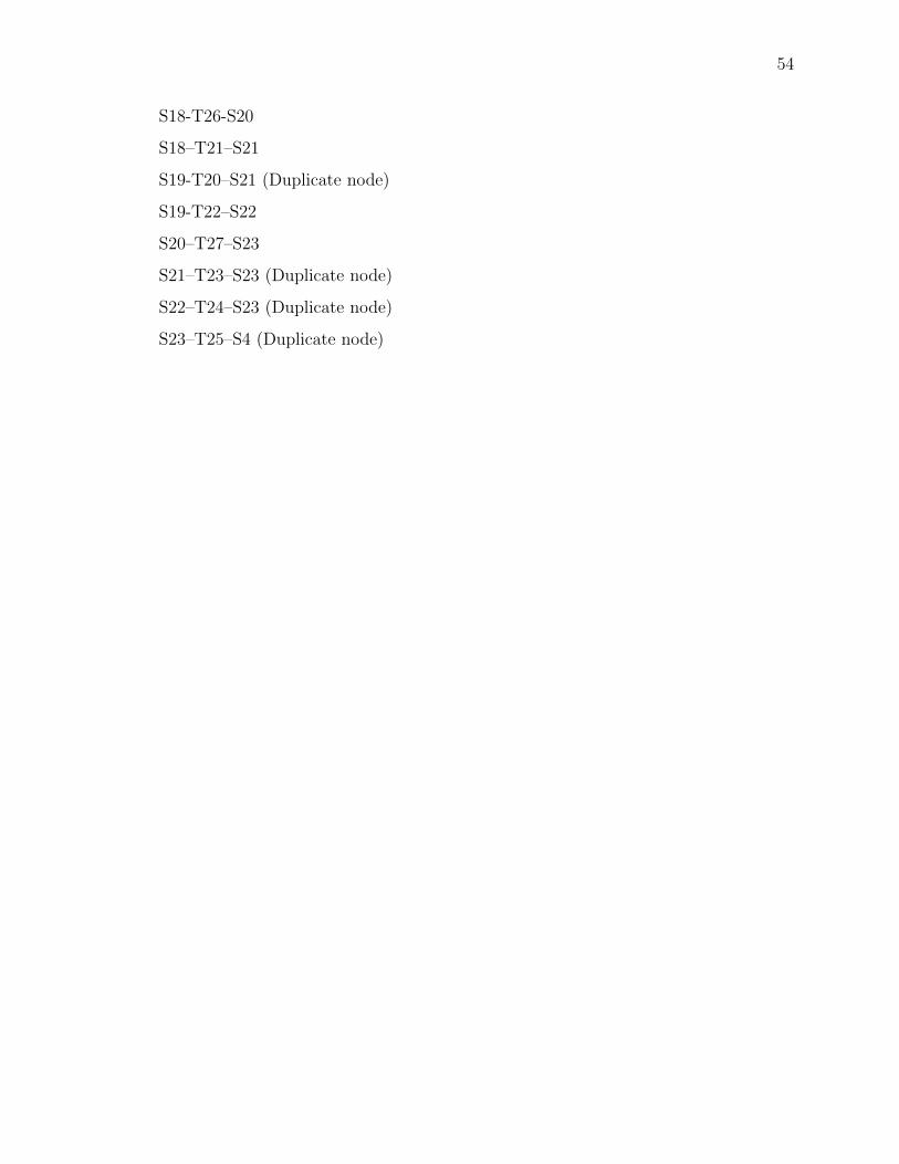
54
S18-T26-S20
S18–T21–S21
S19-T20–S21 (Duplicate node)
S19-T22–S22
S20–T27–S23
S21–T23–S23 (Duplicate node)
S22–T24–S23 (Duplicate node)
S23–T25–S4 (Duplicate node)
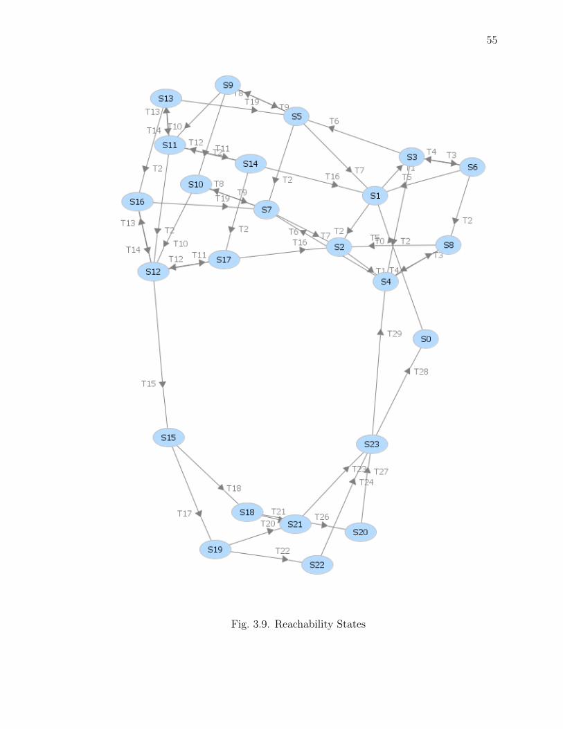
55
Fig. 3.9. Reachability States
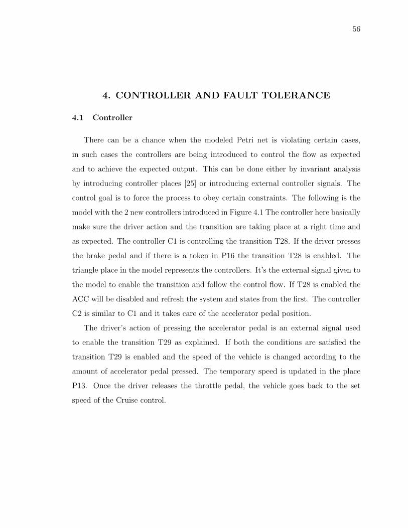
56
4. CONTROLLER AND FAULT TOLERANCE
4.1 Controller
There can be a chance when the modeled Petri net is violating certain cases,
in such cases the controllers are being introduced to control the flow as expected
and to achieve the expected output. This can be done either by invariant analysis
by introducing controller places [25] or introducing external controller signals. The
control goal is to force the process to obey certain constraints. The following is the
model with the 2 new controllers introduced in Figure 4.1 The controller here basically
make sure the driver action and the transition are taking place at a right time and
as expected. The controller C1 is controlling the transition T28. If the driver presses
the brake pedal and if there is a token in P16 the transition T28 is enabled. The
triangle place in the model represents the controllers. It’s the external signal given to
the model to enable the transition and follow the control flow. If T28 is enabled the
ACC will be disabled and refresh the system and states from the first. The controller
C2 is similar to C1 and it takes care of the accelerator pedal position.
The driver’s action of pressing the accelerator pedal is an external signal used
to enable the transition T29 as explained. If both the conditions are satisfied the
transition T29 is enabled and the speed of the vehicle is changed according to the
amount of accelerator pedal pressed. The temporary speed is updated in the place
P13. Once the driver releases the throttle pedal, the vehicle goes back to the set
speed of the Cruise control.
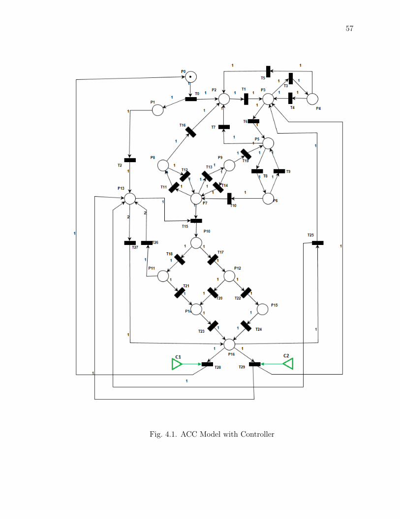
57
Fig. 4.1. ACC Model with Controller

58
The two main control objective considered are,
X1= If the driver move leg from Accelerator pedal to brake
X2= If the driver move leg from brake to Accelerator pedal
C1 =
1, T28 is firing ∧ X1
0, otherwise
(4.1)
C2 =
1, T29 is firing ∧ X2
0, otherwise
(4.2)
The reachable states of the controller action is shown in the figures 4.2 and 4.3.
For example, in figure 4.2 state S23 indicated the controller’s execution. In this state
if the driver action of pressing the throttle pedal is happening and a token in the
place P16 transition T29 is carried out and it reaches the state S24 indicating the
process of continuing the loop for updating the speed in the place P13 and continuous
checking of the vehicle ahead. If the case in figure 4.3 is considered, in the state S23
the controller execution is carried out based on the braking action of the driver and
the token in the place P13 and the transition T28 is enabled to disable the ACC
function and refresh the system.
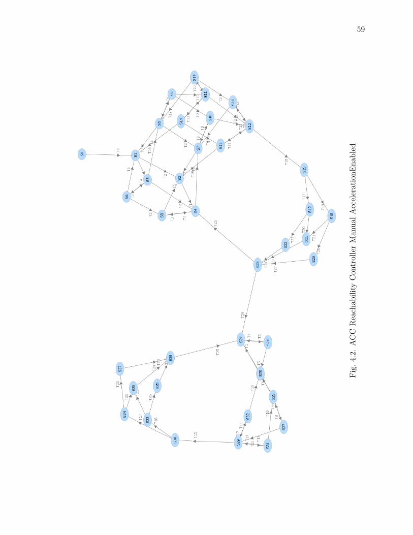
59
Fig
.4.
2.A
CC
Rea
chab
ilit
yC
ontr
olle
rM
anual
Acc
eler
atio
nE
nab
led
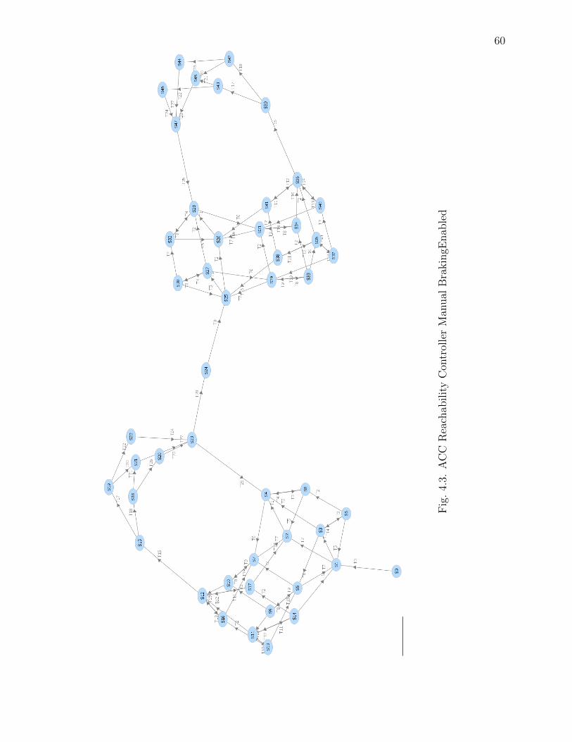
60
Fig
.4.
3.A
CC
Rea
chab
ilit
yC
ontr
olle
rM
anual
Bra
kin
gEnab
led

61
4.2 Fault tolerance Techniques
The fault tolerance techniques is implemented on the controller places introduced
in the model to control the accelerator and brake pedal. In this section fault models
used in the fault detection and identification schemes are discussed. There are two
different fault models, they are Place Fault and Transition Fault [26]. Only place
faults are considered in this research.
Place Fault: A place fault is a case where the token of that single is debased due to
certain actions in the Petri net model. A place fault at time t results in the incorrect
state Mf [t] that can be expressed as,
Mf [t] = M [t]− errorp (4.3)
where M [t] is the state that is supposed to be reached in fault-free conditions and
errorp ε Zn is the place error vector. If the ith entry of errorp is negative, then the
number of tokens in the ith place has been reduced because of the fault; if the token
number is positive, then the token number increased in ith place.
4.2.1 Separate Redundant Petri Net Controllers
A Petri Net controller P c1 and P c2 can be maintained as fault free places using a
separate redundant Petri Net controller. For separate redundant controller new places
and transition are added to the existing model to do the fault tolerance. Basically
linear parity checks are done on the combined marking of the newly added places
and the existing Petri net. This is basic to ensure the redundancy is caught in all
states that should concurrently capture the faults. The detection and identification of
faults in the controlled Petri net system is achieved by adding d places in the original
Petri net controller so that we obtain a separate redundant Petri net controller with
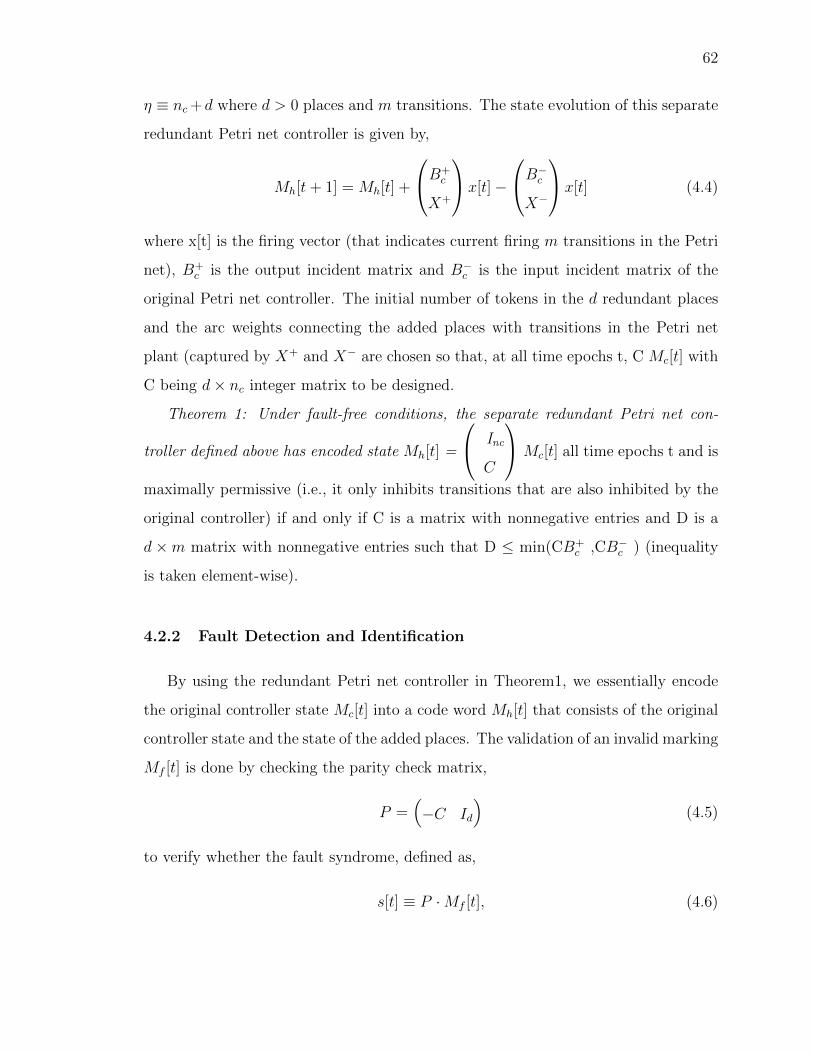
62
η ≡ nc +d where d > 0 places and m transitions. The state evolution of this separate
redundant Petri net controller is given by,
Mh[t+ 1] = Mh[t] +
B+c
X+
x[t]−
B−cX−
x[t] (4.4)
where x[t] is the firing vector (that indicates current firing m transitions in the Petri
net), B+c is the output incident matrix and B−c is the input incident matrix of the
original Petri net controller. The initial number of tokens in the d redundant places
and the arc weights connecting the added places with transitions in the Petri net
plant (captured by X+ and X− are chosen so that, at all time epochs t, C Mc[t] with
C being d× nc integer matrix to be designed.
Theorem 1: Under fault-free conditions, the separate redundant Petri net con-
troller defined above has encoded state Mh[t] =
Inc
C
Mc[t] all time epochs t and is
maximally permissive (i.e., it only inhibits transitions that are also inhibited by the
original controller) if and only if C is a matrix with nonnegative entries and D is a
d ×m matrix with nonnegative entries such that D ≤ min(CB+c ,CB−c ) (inequality
is taken element-wise).
4.2.2 Fault Detection and Identification
By using the redundant Petri net controller in Theorem1, we essentially encode
the original controller state Mc[t] into a code word Mh[t] that consists of the original
controller state and the state of the added places. The validation of an invalid marking
Mf [t] is done by checking the parity check matrix,
P =(−C Id
)(4.5)
to verify whether the fault syndrome, defined as,
s[t] ≡ P ·Mf [t], (4.6)

63
is equal to 0. (This is clearly true under fault-free conditions because Mf [t] = Mh[t]
=
Inc
C
Mc[t] ). For place faults, the fault syndrome at time epoch t is given by,
sp[t] ≡ P ·Mf [t] = P · (Mh[t] + errorP ) = P · errorP (4.7)
and detection and identification is exclusively determined by matrix P. For instance,
to be able to detect and identify a single place fault, we need to choose matrix C such
that any two columns of matrix P are not rational multiples of each other.
Actually, with d redundant places it is possible to simultaneously identify d − 1
transition faults and d/2 place faults.
4.2.3 Detection and Identification of a Single Place Fault
The assumption made here is, there is no transition fault occurred and how the
fault detection and identification is done even there is a fault found in a single place
is discussed. This method can identify the fault in a single place for any Petri net
model. If we choose,
C =
2 1
1 1
(4.8)
the corresponding redundant controller has incident matrix,
Brc =
Bc
C ·Bc
(4.9)
and initial marking M c0 =
IncC
Mc[t]. Note that the choice of matrix C ensures
that the columns of the parity check P are not rational multiples of each other (which
guarantees detection and identification of single place faults).The next step is to
detect and identify a single place fault. The incident matrix of the original controller
is Bc formed with B+c and B−c . The D matrix is of format minimum of B+
c and B−c .
Since the choice of matrix D is not critical in the detection and identification of place
faults, any non-zero matrix can be considered with the corresponding dimensions.
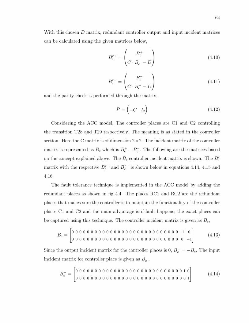
64
With this chosen D matrix, redundant controller output and input incident matrices
can be calculated using the given matrices below,
Br+c =
B+c
C ·B+c −D
(4.10)
Br−c =
B−c
C ·B−c −D
(4.11)
and the parity check is performed through the matrix,
P =(−C I2
)(4.12)
Considering the ACC model, The controller places are C1 and C2 controlling
the transition T28 and T29 respectively. The meaning is as stated in the controller
section. Here the C matrix is of dimension 2×2. The incident matrix of the controller
matrix is represented as Bc which is B+c −B−c . The following are the matrices based
on the concept explained above. The Bc controller incident matrix is shown. The Brc
matrix with the respective Br+c and Br−
c is shown below in equations 4.14, 4.15 and
4.16.
The fault tolerance technique is implemented in the ACC model by adding the
redundant places as shown in fig 4.4. The places RC1 and RC2 are the redundant
places that makes sure the controller is to maintain the functionality of the controller
places C1 and C2 and the main advantage is if fault happens, the exact places can
be captured using this technique. The controller incident matrix is given as Bc,
Bc =
0 0 0 0 0 0 0 0 0 0 0 0 0 0 0 0 0 0 0 0 0 0 0 0 0 0 0 0 −1 0
0 0 0 0 0 0 0 0 0 0 0 0 0 0 0 0 0 0 0 0 0 0 0 0 0 0 0 0 0 −1
(4.13)
Since the output incident matrix for the controller places is 0, B−c = −Bc. The input
incident matrix for controller place is given as B−c ,
B−c =
0 0 0 0 0 0 0 0 0 0 0 0 0 0 0 0 0 0 0 0 0 0 0 0 0 0 0 0 1 0
0 0 0 0 0 0 0 0 0 0 0 0 0 0 0 0 0 0 0 0 0 0 0 0 0 0 0 0 0 1
(4.14)
65
Fig. 4.4. ACC Model with Redundant Controller places

66
The redundant controller incident matrix is formulated as given below,
Brc =
0 0 0 0 0 0 0 0 0 0 0 0 0 0 0 0 0 0 0 0 0 0 0 0 0 0 0 0 −1 0
0 0 0 0 0 0 0 0 0 0 0 0 0 0 0 0 0 0 0 0 0 0 0 0 0 0 0 0 0 −1
0 0 0 0 0 0 0 0 0 0 0 0 0 0 0 0 0 0 0 0 0 0 0 0 0 0 0 0 −2 −1
0 0 0 0 0 0 0 0 0 0 0 0 0 0 0 0 0 0 0 0 0 0 0 0 0 0 0 0 −1 −1
(4.15)
The output incident matrix of redundant controller is calculated as,
Br+c =
0 0 0 0 0 0 0 0 0 0 0 0 0 0 0 0 0 0 0 0 0 0 0 0 0 0 0 0 0 0
0 0 0 0 0 0 0 0 0 0 0 0 0 0 0 0 0 0 0 0 0 0 0 0 0 0 0 0 0 0
0 0 0 0 0 0 0 0 0 0 0 0 0 0 0 0 0 0 0 0 0 0 0 0 0 0 0 0 0 0
−1 0 0 0 0 0 0 0 0 0 0 0 0 0 0 0 0 0 0 0 0 0 0 0 0 0 0 0 0 0
(4.16)
The input incident matrix of redundant controller is calculated as,
Br−c =
0 0 0 0 0 0 0 0 0 0 0 0 0 0 0 0 0 0 0 0 0 0 0 0 0 0 0 0 1 0
0 0 0 0 0 0 0 0 0 0 0 0 0 0 0 0 0 0 0 0 0 0 0 0 0 0 0 0 0 1
0 0 0 0 0 0 0 0 0 0 0 0 0 0 0 0 0 0 0 0 0 0 0 0 0 0 0 0 2 1
−1 0 0 0 0 0 0 0 0 0 0 0 0 0 0 0 0 0 0 0 0 0 0 0 0 0 0 0 1 1
(4.17)
The default D matrix is considered here,
D =
0 0 0 0 0 0 0 0 0 0 0 0 0 0 0 0 0 0 0 0 0 0 0 0 0 0 0 0 0 0
1 0 0 0 0 0 0 0 0 0 0 0 0 0 0 0 0 0 0 0 0 0 0 0 0 0 0 0 0 0
(4.18)
Then the decoding of the matrix is done by calculating PMf [t]. If the result is a
multiple of
2
1
1
1
1
0
0
1
then the place Pc1, Pc2, Rc1, Rc2 respectively has
suffered a place fault.
4.3 Failure cases
The failure of Adaptive cruise control system can happen due to various reasons.
The technology failure can be software, hardware or the interface.
4.3.1 Failure due to Driver response or hardware
Failure of the technology or system can be faced at any situation due to different
reasons. The driver response to the system is an area of research carried out for all
67
ADAS to analyze drivers comfort and problems for the betterment of the technology.
In reference it explains how to determine whether drivers who are using ACC in
their personal vehicle respond appropriately to the feedback provided by a familiar
ACC system under crash-likely scenarios and to analyze if there are any error patter
followed by the drivers that might have impact the safety issues and how to find a
countermeasures if there are any safety-critical errors made by the drivers by misuse
of the system. The main area of research to be concerned on driver response are the
HMI and driver psychology. The knowledge on this helps to write the criteria for
enabling the transition and to decide the number of tokens to be put in a place.
The hardware failure like brake, accelerator, loss of steering control, worn out CC
ON/OFF switch and engine stall suddenly due to certain cause comes under the tree
of cruise control system failure due to hardware issues. This is rarely caused and it
is common for all features in the car.
4.3.2 Model failure
Petri nets comes under visualizing the working of the software designed according
to the control flow. If there are any parameters not set accordingly or if there are
any calibration issue, the system might not work as expected and it can be figured
out while simulating the Petri net model. If a certain transition is not triggered, the
inputs and the enabling condition can be checked to find the root cause of the issue.
For example, let us consider the case of RADAR sensor. For RADAR the bandwidth
is set in the calibration for the detection of the vehicle in the front. If there is a
fault in the calibration i.e, if some parameter is not set accordingly, the transition
T8 won’t be enabled and the place P6 will never get a token unless the calibration
is set properly. This case is considered as the system failure. There can be others
situation like various noises affecting the model that leads to system failure. This
noise can affect places like Cruise speed updates, detection of objects using RADAR
or any other sensors or even in the response time of switching ON/OFF of Cruise

68
control button. Suppose due to fault, there are 2 tokens placed in the place P16, if
the transition T28 and T29 will happen next to next which will deploy the system
by sending signal to both brake and accelerator leading to failure of the system and
fatal issues. These cases should be controlled accordingly.
69
5. CONCLUSION AND FUTURE WORK
5.1 Conclusion
The Petri net model of the feature ACC is designed and analyzed based on the
various functionality like place invariant, transition invariant and reachability tree.
Then the fault tolerant techniques are implemented on the controller places intro-
duced for controlling the brake and accelerator actions. So if there is a transient fault
in the Petri net model, the fault causing place can be identified using this techniques
mentioned in this research. According to the analysis carried out in 2017, the ACC
system is simulated in Matlab and Simulink considering various cases and the prob-
abilities of a collision and a near miss were computed based on regular test cases
and critical test cases [2]. The ACC system working in mixed traffic is analyzed for
better stability [16]. The various other ongoing research on ACC and CACC helps in
improvement of the model and safety.
5.2 Future Work
5.2.1 Hybrid PetriNet model Integration
The discrete model of Adaptive cruise control logic is discussed considering all
states and transitions as discrete events. To observe the dynamics of the vehicle
in the Petri net flow, hybrid Petri net can be used. The dynamic places can be
represented as continuous places and the event driven can be discrete places. In the
discrete model the places that represents speed, distance, set speed, adjust speed
are considered as continuous places and the model should be modified accordingly.
There might be few discrepancies in the model due to the looping methodology and
newly introduced continuous places. Like the place P3 in figure 3.8, that takes the
70
manual speed continuously for every iteration and it is replaced by the new adjusted
set speed for every iteration if the car is detected. In this scenario, since the tokens
in P3 are real time numbers we cannot define the weight of the arc for the transition
to happen. For these cases Timed Petri Nets and colored Petri nets comes into
picture [27]. The model can also be improvised by considering the cut-in vehicle
scenarios for betterment of safety [28].
5.2.2 SimHPN tool
Since the reachability tree for continuous and hybrid model cannot be achieved
using reachability algorithm, a simulation tool called SimHPN can be used. It is a
GUI for the users to simulate and analyze the Petri net models. This tool basically is
an add on tool in Matlab with the control panels for simulations and carry out analysis
methods. The Menu bar has different features available in the SimHPN toolbox as
Model, Options, Simulation, Discrete, Continuous and Hybrid for specified model
analysis [29].
5.2.3 Interface with other safety features
As ACC is an active safety feature, it can be interfaced with other safety features
like lane control, blind spot warning, lane change warning for the better protection
of car and leading to the scope of autonomous vehicles. Petri nets being a graphical
tool, system behavior can be easily depicted through mathematical firing equations.

REFERENCES
71
REFERENCES
[1] L. Luo, “Adaptive cruise control design with consideration of humans’ drivingpsychology,” in 2014 11th World Congress on Intelligent Control and Automation(WCICA). IEEE, 2014, pp. 2973–2978.
[2] E. de Gelder and J.-P. Paardekooper, “Assessment of automated driving systemsusing real-life scenarios,” in Intelligent Vehicles Symposium (IV), 2017 IEEE.IEEE, 2017, pp. 589–594.
[3] Y.-C. Lin, H.-C. Hsu, and I.-C. Kuo, “An eco-cruising control systems using non-linear predictive control approach,” in Automatic Control Conference (CACS),2016 International. IEEE, 2016, pp. 59–64.
[4] I. Kılıc, A. Yazıcı, O. Yıldız, M. Ozcelikors, and A. Ondogan, “Intelligent adap-tive cruise control system design and implementation,” in System of SystemsEngineering Conference (SoSE), 2015 10th. IEEE, 2015, pp. 232–237.
[5] P. Shakouri, A. Ordys, D. S. Laila, and M. Askari, “Adaptive cruise control sys-tem: comparing gain-scheduling pi and lq controllers,” IFAC Proceedings Vol-umes, vol. 44, no. 1, pp. 12 964–12 969, 2011.
[6] W. Pananurak, S. Thanok, and M. Parnichkun, “Adaptive cruise control for anintelligent vehicle,” in ROBIO 2008. IEEE International Conference on Roboticsand Biomimetics, 2008. IEEE, 2009, pp. 1794–1799.
[7] G. Naus, R. Van Den Bleek, J. Ploeg, B. Scheepers, R. van de Molengraft, andM. Steinbuch, “Explicit mpc design and performance evaluation of an acc stop-&-go,” in American Control Conference, 2008. IEEE, 2008, pp. 224–229.
[8] E. de Gelder, I. Cara, J. Uittenbogaard, L. Kroon, S. van Iersel, and J. Hogema,“Towards personalised automated driving: Prediction of preferred acc behaviourbased on manual driving,” in Intelligent Vehicles Symposium (IV), 2016 IEEE.IEEE, 2016, pp. 1211–1216.
[9] D. Gruyer, S. Pechberti, and S. Glaser, “Development of full speed range acc withsivic, a virtual platform for adas prototyping, test and evaluation,” in IntelligentVehicles Symposium Workshops (IV Workshops), 2013 IEEE. IEEE, 2013, pp.93–98.
[10] H. Eom and S. H. Lee, “Human-automation interaction design for adaptive cruisecontrol systems of ground vehicles,” Sensors, vol. 15, no. 6, pp. 13 916–13 944,2015.

72
[11] A. Validi, T. Ludwig, and C. Olaverri-Monreal, in Vehicular Electronics andSafety (ICVES), 2017 IEEE International Conference on Analyzing the effectsof V2V and ADAS-ACC penetration rates on the level of road safety in inter-sections: Evaluating simulation platforms SUMO and scene suite. IEEE, 2017,pp. 38–43.
[12] C. G. Cassandras and S. Lafortune, Introduction to discrete event systems.Springer Science & Business Media, 2009.
[13] H. Alla and R. David, “Continuous and hybrid petri nets,” Journal of Circuits,Systems, and Computers, vol. 8, no. 01, pp. 159–188, 1998.
[14] R. David and H. Alla, “Autonomous and timed continuous petri nets,” in Inter-national Conference on Application and Theory of Petri Nets. Springer, 1991,pp. 71–90.
[15] T. Litman, Autonomous vehicle implementation predictions. Victoria TransportPolicy Institute, 2017.
[16] S. Kitazono and H. Ohmori, “Semi-autonomous adaptive cruise control in mixedtraffic,” in SICE-ICASE, 2006. International Joint Conference. IEEE, 2006,pp. 3240–3245.
[17] J. Wang and R. Rajamani, “Should adaptive cruise-control systems be designedto maintain a constant time gap between vehicles?” IEEE Transactions on Ve-hicular Technology, vol. 53, no. 5, pp. 1480–1490, 2004.
[18] G. W. Stimson, “Airborne radar,” New Jersey: SciTech, pp. 317–322, 1998.
[19] S. Y. P. S. Kumar, Avinash, “A review paper on radar system.” National Confer-ence on Innovations in Micro-electronics, Signal Processing and CommunicationTechnologies, 2016.
[20] M. A. Richards, Fundamentals of radar signal processing. Tata McGraw-HillEducation, 2005.
[21] J. Moeckli, T. Brown, B. Dow, L. N. Boyle, C. Schwarz, and H. Xiong, “Evalu-ation of adaptive cruise control interface requirements on the national advanceddriving simulator,” Tech. Rep., 2015.
[22] A. S. Staines, “Modeling and analysis of a cruise control system,” World Academyof Science, Engineering and Technology, vol. 38, pp. 173–177, 2008.
[23] S. Duan and J. Zhao, in Image, Vision and Computing (ICIVC), 2017 2nd Inter-national Conference on A model based on hierarchical safety distance algorithmfor ACC control mode switching strategy.
[24] B. Breimer, Design of an Adaptive Cruise Control Model for Hybrid SystemsFault Diagnosis. PhD Dissertation, McMaster University, 2013.
[25] K. Yamalidou, J. Moody, M. Lemmon, and P. Antsaklis, “Feedback control ofpetri nets based on place invariants,” Automatica, vol. 32, no. 1, pp. 15–28, 1996.
[26] L. Li, C. N. Hadjicostis, and R. Sreenivas, in Decision and Control, 2004. CDC.43rd IEEE Conference on Fault detection and identification in Petri net con-trollers, vol. 5. IEEE, 2004, pp. 5248–5253.
73
[27] N. Wu, F. Chu, S. Mammar, and M. Zhou, in Networking, Sensing and Control(ICNSC), 2011 IEEE International Conference on Interaction behavior modelingof advanced driving assistance systems by using Petri net. IEEE, 2011, pp. 145–150.
[28] I. Dagli, G. Breuel, H. Schittenhelm, and A. Schanz, “Cutting-in vehicle recog-nition for acc systems-towards feasible situation analysis methodologies,” in In-telligent Vehicles Symposium, 2004 IEEE. IEEE, 2004, pp. 925–930.
[29] J. Julvez and C. Mahulea, “Simhpn: A matlab toolbox for hybrid petri nets,”User Manual, 2012.