Adaptive Cruise Control and Driver Modeling Cruise Control and Driver Modeling ... itself from...
91
Adaptive Cruise Control and Driver Modeling Johan Bengtsson Department of Automatic Control Lund Institute of Technology Lund, November 2001
Transcript of Adaptive Cruise Control and Driver Modeling Cruise Control and Driver Modeling ... itself from...
Adaptive Cruise Control andDriver Modeling
Johan Bengtsson
Department of Automatic ControlLund Institute of Technology
Lund, November 2001
Department of Automatic ControlLund Institute of TechnologyBox 118S-221 00 LUNDSweden
ISSN 0280–5316ISRN LUTFD2/TFRT--3227--SE
c&2001 by Johan Bengtsson. All rights reserved.Printed in Sweden,Lund University, Lund 2001
Contents
Acknowledgments . . . . . . . . . . . . . . . . . . . . . . . . 71. Introduction . . . . . . . . . . . . . . . . . . . . . . . . . . 8
1.1 Background and Motivation . . . . . . . . . . . . . . 82. Review of driver models . . . . . . . . . . . . . . . . . . 10
2.1 Introduction . . . . . . . . . . . . . . . . . . . . . . . . 102.2 Human driver models . . . . . . . . . . . . . . . . . . 102.3 General longitudinal driver behavior . . . . . . . . . 202.4 The human driver brake behavior . . . . . . . . . . . 262.5 Safety . . . . . . . . . . . . . . . . . . . . . . . . . . . 272.6 Existing systems . . . . . . . . . . . . . . . . . . . . . 292.7 Cut in Situations . . . . . . . . . . . . . . . . . . . . . 312.8 Activities and WWW-links . . . . . . . . . . . . . . . 31
3. Material & Methods . . . . . . . . . . . . . . . . . . . . . . 333.1 Introduction . . . . . . . . . . . . . . . . . . . . . . . . 333.2 Experimental platform . . . . . . . . . . . . . . . . . 343.3 Experimental design . . . . . . . . . . . . . . . . . . . 373.4 System identification . . . . . . . . . . . . . . . . . . . 453.5 Transposed data . . . . . . . . . . . . . . . . . . . . . 563.6 Driver modeling using neural networks . . . . . . . . 57
4. Validation & Results . . . . . . . . . . . . . . . . . . . . . 594.1 Introduction . . . . . . . . . . . . . . . . . . . . . . . . 594.2 Linear regression . . . . . . . . . . . . . . . . . . . . . 614.3 Subspace-based identification . . . . . . . . . . . . . . 664.4 Behavioral model . . . . . . . . . . . . . . . . . . . . . 74
5

Contents
4.5 Detection and modeling of changed driver behavior . 794.6 Neural network modeling . . . . . . . . . . . . . . . . 814.7 Summary . . . . . . . . . . . . . . . . . . . . . . . . . 83
5. Discussion & Conclusions . . . . . . . . . . . . . . . . . . 855.1 Discussion . . . . . . . . . . . . . . . . . . . . . . . . . 855.2 Conclusions . . . . . . . . . . . . . . . . . . . . . . . . 88
6. Bibliography . . . . . . . . . . . . . . . . . . . . . . . . . . 89
6

Acknowledgments
Acknowledgments
First of all, I would like to thank my supervisor Rolf Johansson for hisguidance and for many stimulating discussions. It is a pleasure to workat the Dept. of automatic Control consisting of talented people, goodfacilities and a great atmosphere. Therefore, I would like to thank youall. I would specially want thank Bo Lincoln and Anders Robertsson.
At Volvo Technical Development I would like to thank Agneta Sjö-gren, Eric Hesslow and Fredrik Botling for the assistance and help. Ialso want to thank Mathias Haage at Dept. Computer science, LundInstitute of Technology whose comments on my work have been valu-able.
This work has been supported by Volvo Technical Development andVINNOVA (Swedish Agency for Innovation Systems) formerly calledNUTEK (Swedish National board for Industrial and Technical Devel-opment).
Johan Bengtsson
7
1
Introduction
1.1 Background and Motivation
Systems that support a driver in traffic situations and reduce the totaldriver workload, is a growing research topic. Several of these sup-port systems aim toward full or partial automatic driver assistance,such as those for longitudinal control that are often called AdaptiveCruise Control (ACC) systems. Adaptive cruise control distinguishesitself from cruise control in its use of sensors that measure the head-way distance and a controller which adjusts the velocity and distanceto the vehicle in front. Adaptive cruise control requires appropriatesensor technology, actuators and control devices and its system designrequires data acquisition, control system design and validation proce-dures. The motivation for these systems is that they aim at increasingthe driving comfort, reducing traffic accidents and increasing the trafficflow throughput. The ACC systems autonomously adjust the vehicle’sspeed according to current driving conditions. In order to accomplishdriver comfort the system must resemble driver behavior in traffic.The system must avoid irritation of the driver and of the surroundingtraffic. Therefore, to design a system that resembles the natural longi-tudinal behavior of a driver a good model is needed. There exist severalattempts to model the drivers’ longitudinal behavior, which all aim atdescribing various parts of the drivers’ behavior. The model structuresare different, some are based on cognitive models or general longitudi-
8
1.1 Background and Motivation
nal models or only car-following models. Most of them have one thingin common in that they are using static models.
The main contributions of the thesis are:
• An experimental platform for adaptive cruise control and drivermodeling;
• Contribution to the description of human driver’s longitudinaldriver behavior using dynamic models;
• The use of system identification methods to obtain the drivermodels useful for adaptive cruise control.
Experiments in which seven drivers participated have been per-formed for a variety of different traffic situations. The collected datahave been analyzed and used in the estimation of the driver models.
9
2
Review of driver models
2.1 Introduction
Human driver behavior has been studied since the beginning of the1950s, but during the 1990s the topic has grown considerably.
The division of driver behavior into separately studied parts hasbeen a common theme of the field, since a general driver model is inher-ently complex. For example, there exist separate models for describingsteering behavior, driver work load, safety behavior and longitudinalbehavior.
This chapter concentrates on a review of different longitudinal be-havior models. A longitudinal model describes vehicle acceleration be-havior using throttle and brakes as input signals.
2.2 Human driver models
The study of the human driver behavior in car-following situationsstarted in the 1950s and has since been an extended topic. The generalform of the car-following driver models developed in the 1950s is basedon the assumption that each driver reacts in a specific fashion to astimulus, which leads to an actuation of the acceleration. Stimulus maybe a change in the headway distance or a change in the environmentcondition.
10
2.2 Human driver models
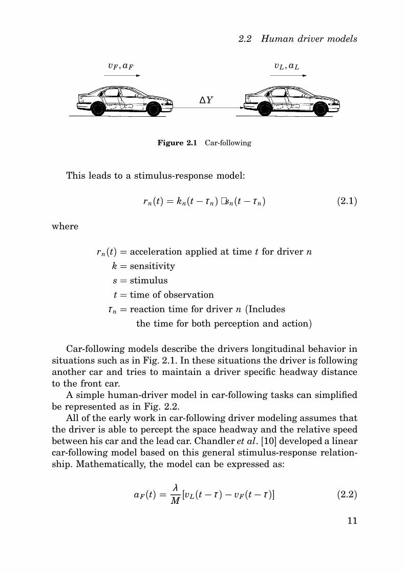
vF , aF vL, aL
∆Y
Figure 2.1 Car-following
This leads to a stimulus-response model:
rn(t) = kn(t −τ n) ⋅ sn(t − τ n) (2.1)
where
rn(t) = acceleration applied at time t for driver n
k = sensitivity
s = stimulus
t = time of observation
τ n = reaction time for driver n (Includes
the time for both perception and action)
Car-following models describe the drivers longitudinal behavior insituations such as in Fig. 2.1. In these situations the driver is followinganother car and tries to maintain a driver specific headway distanceto the front car.
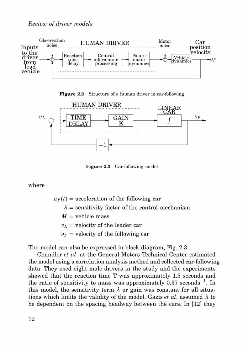
A simple human-driver model in car-following tasks can simplifiedbe represented as in Fig. 2.2.
All of the early work in car-following driver modeling assumes thatthe driver is able to percept the space headway and the relative speedbetween his car and the lead car. Chandler et al. [10] developed a linearcar-following model based on this general stimulus-response relation-ship. Mathematically, the model can be expressed as:
aF(t) = λM[vL(t −τ ) − vF(t− τ )] (2.2)
11
Review of driver models
vF
HUMAN DRIVER
Reactiontimedelay
Centralinformationprocessing
Neuromotor
dynamicsVehicle
dynamics
Motornoisenoise
Observation
Inputsto thedriverfromlead
vehicle
Carpositionvelocity∑∑
Figure 2.2 Structure of a human driver in car-following
vL
HUMAN DRIVER
TIMEDELAY
−1
GAINK
LINEARCAR∫ vF
Figure 2.3 Car-following model
where
aF(t) = acceleration of the following car
λ = sensitivity factor of the control mechanism
M = vehicle mass
vL = velocity of the leader car
vF = velocity of the following car
The model can also be expressed in block diagram, Fig. 2.3.Chandler et al. at the General Motors Technical Center estimated
the model using a correlation analysis method and collected car-followingdata. They used eight male drivers in the study and the experimentsshowed that the reaction time T was approximately 1.5 seconds andthe ratio of sensitivity to mass was approximately 0.37 seconds−1. Inthis model, the sensitivity term λ or gain was constant for all situa-tions which limits the validity of the model. Gazis et al. assumed λ tobe dependent on the spacing headway between the cars. In [12] they
12
2.2 Human driver models
developed the following model:
aF(t) = b∆Y(t −τ ) (vL(t− τ ) − vF(t − τ )) (2.3)
where
b = sensitivity constant
∆Y(t− τ ) = the space headway at time (t −τ )
As this model had limitations in low density traffic Edie et al. [11]proposed a new model:
aF(t) = bvL(t −τ )
∆Y(t− τ )2 (vL(t −τ ) − vF(t −τ )) (2.4)
This model performs better than the model proposed by Gazis etal. [12] at low traffic densities. Gazis et al. [13] developed a modelthat would be known as the General Motors Nonlinear (GM) model.Mathematically the model can be expressed as:
aF(t) = αvL(t)β
∆Y(t −τ )γ (vL(t− τ ) − vF(t− τ )) (2.5)
where
α = constant
β = model parameter
γ = model parameter
Gazis et al. tried to estimate the model, but they had not sufficientdata to claim a certain model to be superior to all others. May andKeller [38] made a rigorous framework to estimate the GM model. Inthe Gazis et al [13] study, β and γ were integers but in the May Keller[38] study the β and γ were allowed to be real values. They found thatα = 1.33e-4, β = 0.8, and γ = 2.8 gave higher correlation between theobserved and estimated accelerations.
13
Review of driver models
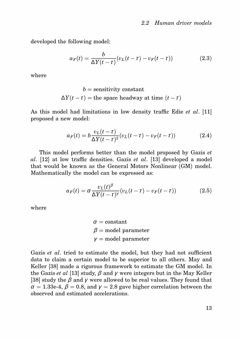
θ
Figure 2.4 The visual angle in car-following
Pipes [42] developed an alternative approach, which is based on theassumption that a driver is using the visual angle enclosing the leadcar (Fig 2.4).
The angle θ increases when the following car is approaching thelead car. Using this approach, Pipe developed a model where the ac-celeration of the following car is proportional to the driver’s perceptionof the rate of change of the visual angle θ . Expressed mathematically:
aF(t) = b(vL(t − τ ) − vF(t − τ ))
(∆Y(t −τ ))2 (2.6)
Addison and Low [1] developed a model based on the assumptionthat the driver aims at a desired headway and strives to minimize therelative speed ∆v. The model is an extension of the Gazis et al. [13]including a nonlinear headway-dependent term. Mathematically, themodel can be expressed as:
an(t) = αvf (t)β ∆v(t − τ )(∆Y(t −τ ))γ +η(∆Y(t − τ ) − Dn)3 (2.7)
where
Dn = the desired headway
η = constant
Linear Optimal Control Model Structure
The optimal control model structure is based on a performance crite-rion such as that of linear quadratic Gaussian control [3]. Minimizationof the performance criteria gives the structure of the controller. Thisstructure differs from the stimulus-response structure, since nonlin-earities in the vehicle are included in the model. Bekey [4], who madea review on this model structure, mentioned that even though it maynot be reasonable to assume that a human driver should mimic anoptimal controller, the result is interesting.
14
2.2 Human driver models
SWITCHING
LOGIC
∫vF
K1
K2
aF1
aF2
aF3
∑∑vF1
vF2
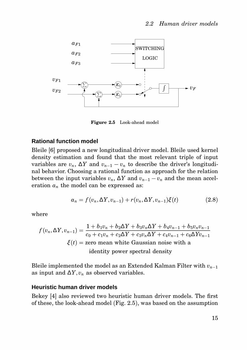
Figure 2.5 Look-ahead model
Rational function model
Bleile [6] proposed a new longitudinal driver model. Bleile used kerneldensity estimation and found that the most relevant triple of inputvariables are vn, ∆Y and vn−1 − vn to describe the driver’s longitudi-nal behavior. Choosing a rational function as approach for the relationbetween the input variables vn, ∆Y and vn−1 − vn and the mean accel-eration an the model can be expressed as:
an = f (vn, ∆Y , vn−1) + r(vn, ∆Y , vn−1)ξ (t) (2.8)
where
f (vn, ∆Y , vn−1) = 1+ b1vn + b2∆Y + b3vn∆Y + b4vn−1 + b5vnvn−1
c0 + c1vn + c2∆Y + c3vn∆Y + c4vn−1 + c6∆Yvn−1
ξ (t) = zero mean white Gaussian noise with a
identity power spectral density
Bleile implemented the model as an Extended Kalman Filter with vn−1
as input and ∆Y , vn as observed variables.
Heuristic human driver models
Bekey [4] also reviewed two heuristic human driver models. The firstof these, the look-ahead model (Fig. 2.5), was based on the assumption
15
Review of driver models
that the driver observes the behavior of three cars ahead of him, andthat he adjust his own strategy from their behavior. The second model,a finite-state model, is based on the assumption that a human driveralways tries to maintain a velocity equal to the lead car along a safeheadway.
Adaptive Cruise Control
Ioannou [25] presented an ACC system, which he compared to threehuman driver models: Linear car-follow model, Linear Optimal ControlModel, and Look-ahead Model. Mathematically, the vehicle model canbe expressed as:
ddt
yn(t) = vn(t)ddt
yn(t) = an(t)ddt
yn(t) = b( yn, yn) +α ( yn)un(t)
where
α ( yn) = 1mnτ n( yn)
b( yn, yn) = −2kdn
mnyn yn − 1
τ n( yn) [ yn + kdn
mny2
n +dmn( yn)
mn]
yn = position of the nth vehicle
vn = velocity of the nth vehicle
an = acceleration of the nth vehicle
mn = mass of the nth vehicle
τ n = nth vehicle’s engine time constant
un = nth vehicle’s engine input
kdn = nth aerodynamic drag coefficient
dmn = mechanical drag of the nth vehicle
Control law:
un = 1α ( yn) [cn(t) − b( yn, yn)] (2.9)
16
2.2 Human driver models
where
cn = Cpδ n(t) + Cuδ n(t) + Kvvn(t) + Kaan(t)δ n(t) = yn−1(t) − yn − (Ln + Son + λ2vn(t))δ n(t) = vn−1(t) − vn − λ2an(t)
Ln = length of the nth vehicle
Son = initial headway
δ n(t) = deviation from desired headway
Cp = design constant
Cv = design constant
Kv = design constant
Ka = design constant
Ioannou’s conclusion was that the comparison indicates a strong po-tential for ACC to smoothen traffic flows and to increase traffic flowrates considerably if designed and implemented properly. In this studyseveral emergency situations were simulated and used to demonstratethat the ACC proposed may lead to much safer driving. This ACCmodel is the foundation for the ACC system now used by Ford.
Neural network and fuzzy logic model.
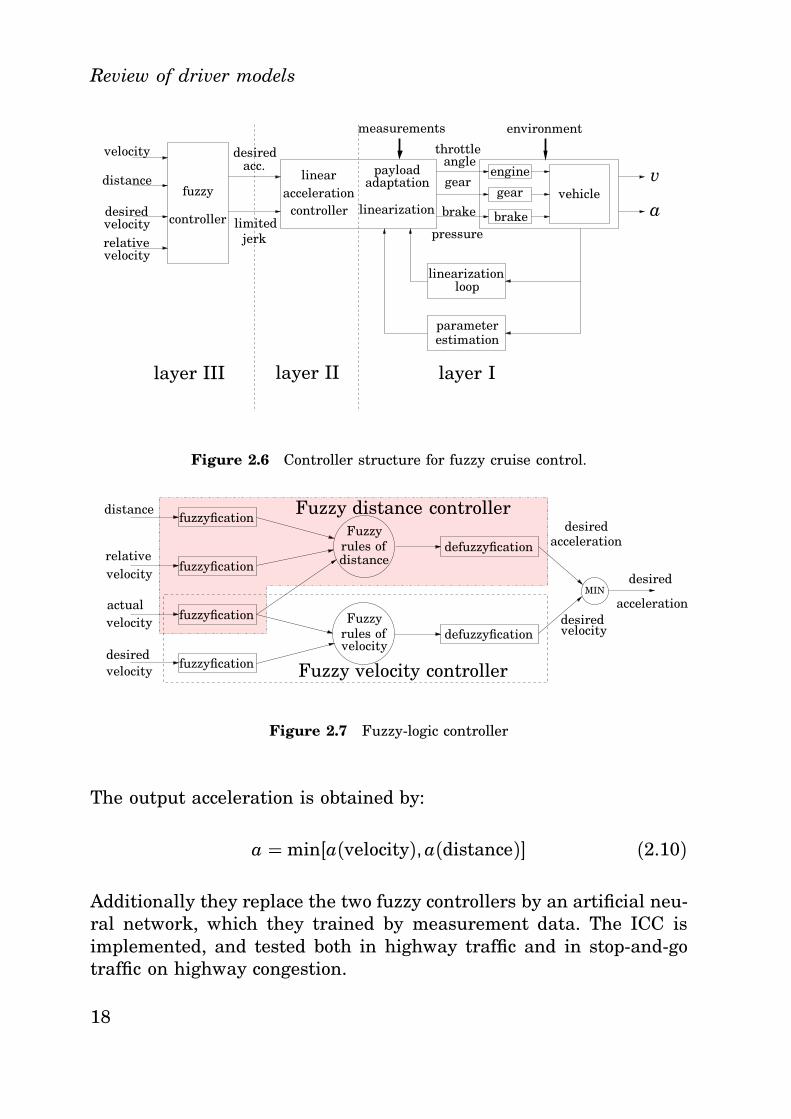
Ghazi Zadeh et al. [15] made a literature survey on this area. Thedriver models presented in the review all handle lateral guidance andsome of them also include longitudinal guidance. Several of the drivermodels in the survey are for autonomous vehicle following, e.g., Gris-wold [19]. Germann and Isermann [14] proposed an intelligent cruisecontrol (ICC) based on fuzzy logic and neural networks. They use athree-layer structure, Fig. 2.6.
In the first layer, a linearization of the nonlinearities is made. Thesecond layer consists of a linear acceleration controller, based on clas-sical controlling techniques and the third layer consist of a fuzzy con-troller, based on the linguistic description of comfort demands.
The fuzzy controller (Fig 2.7) is based on the different ‘linguistic’input variables: distance, velocity, relative velocity, and actual velocity.
17
Review of driver models
velocity
velocity
velocity
distance
desired
desired
relative
fuzzy
controllercontroller
linear payload
acceleration
acc.adaptation
linearization
linearization
throttleangle
geargear
brakebrake
pressure
engine
vehicle
loop
parameterestimation
environmentmeasurements
layer Ilayer IIlayer III
limitedjerk
v
a
Figure 2.6 Controller structure for fuzzy cruise control.
velocityvelocity
velocity
velocity
velocity
distance
distance
desired
desired
desired
desired
acceleration
acceleration
actualMIN
Fuzzy
Fuzzy
relative
rules of
rules of
fuzzyfication
fuzzyfication
fuzzyfication
fuzzyfication
defuzzyfication
defuzzyfication
Fuzzy distance controller
Fuzzy velocity controller
Figure 2.7 Fuzzy-logic controller
The output acceleration is obtained by:
a = min[a(velocity), a(distance)] (2.10)
Additionally they replace the two fuzzy controllers by an artificial neu-ral network, which they trained by measurement data. The ICC isimplemented, and tested both in highway traffic and in stop-and-gotraffic on highway congestion.
18
2.2 Human driver models
supervisoryagent
longitudinalvehicle vehiclecontrol control
lateral use
car phone
SR TR BA
KB behavior
RB behavior
SB behavior
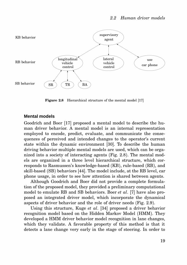
Figure 2.8 Hierarchical structure of the mental model [17]
Mental models
Goodrich and Boer [17] proposed a mental model to describe the hu-man driver behavior. A mental model is an internal representationemployed to encode, predict, evaluate, and communicate the conse-quences of perceived and intended changes to the operator’s currentstate within the dynamic environment [30]. To describe the humandriving behavior multiple mental models are used, which can be orga-nized into a society of interacting agents (Fig. 2.8). The mental mod-els are organized in a three level hierarchical structure, which cor-responds to Rasmussen’s knowledge-based (KB), rule-based (RB), andskill-based (SB) behaviors [44]. The model include, at the RB level, carphone usage, in order to see how attention is shared between agents.
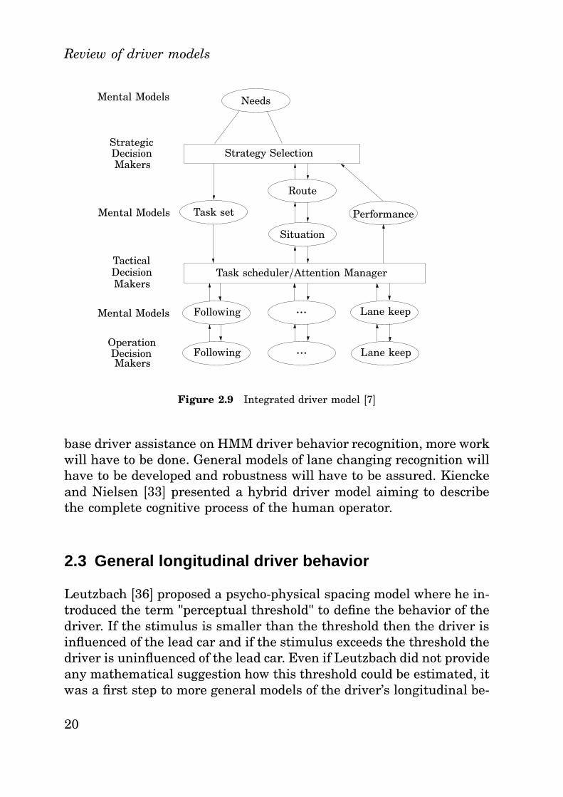
Although Goodrich and Boer did not provide a complete formula-tion of the proposed model, they provided a preliminary computationalmodel to emulate RB and SB behaviors. Boer et al. [7] have also pro-posed an integrated driver model, which incorporate the dynamicalaspects of driver behavior and the role of driver needs (Fig. 2.9).
Using this structure, Kuge et al. [34] proposed a driver behaviorrecognition model based on the Hidden Markov Model (HMM). Theydeveloped a HMM driver behavior model recognition in lane changes,which they validate. A favorable property of this method is that itdetects a lane change very early in the stage of steering. In order to
19
Review of driver models
Mental Models
Strategic
Decision
Decision
Decision
Makers
Makers
Makers
Mental Models
Mental Models
Tactical
Operation
Needs
Strategy Selection
Task set
Route
Situation
Performance
Task scheduler/Attention Manager
Following
Following ...
... Lane keep
Lane keep
Figure 2.9 Integrated driver model [7]
base driver assistance on HMM driver behavior recognition, more workwill have to be done. General models of lane changing recognition willhave to be developed and robustness will have to be assured. Kienckeand Nielsen [33] presented a hybrid driver model aiming to describethe complete cognitive process of the human operator.
2.3 General longitudinal driver behavior
Leutzbach [36] proposed a psycho-physical spacing model where he in-troduced the term "perceptual threshold" to define the behavior of thedriver. If the stimulus is smaller than the threshold then the driver isinfluenced of the lead car and if the stimulus exceeds the threshold thedriver is uninfluenced of the lead car. Even if Leutzbach did not provideany mathematical suggestion how this threshold could be estimated, itwas a first step to more general models of the driver’s longitudinal be-
20
2.3 General longitudinal driver behavior
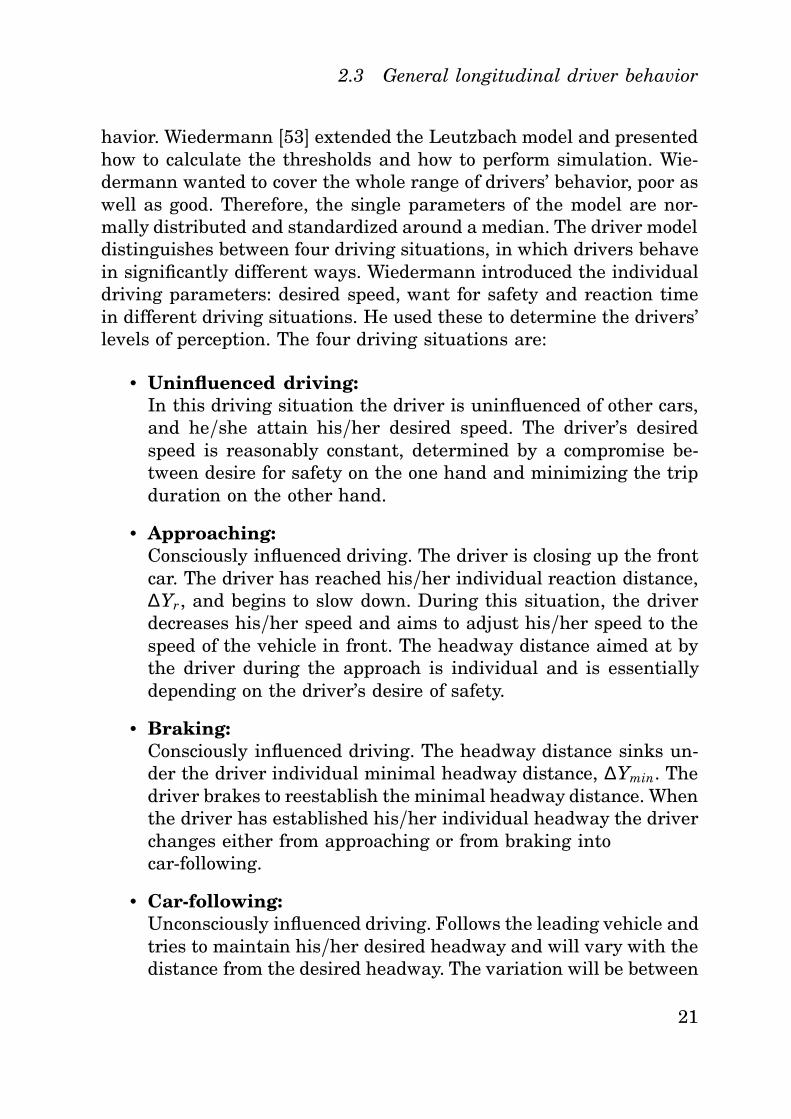
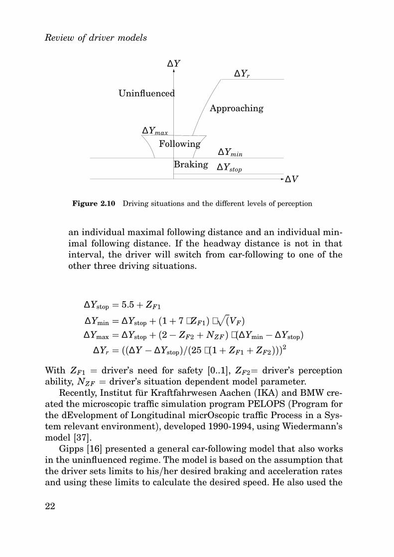
havior. Wiedermann [53] extended the Leutzbach model and presentedhow to calculate the thresholds and how to perform simulation. Wie-dermann wanted to cover the whole range of drivers’ behavior, poor aswell as good. Therefore, the single parameters of the model are nor-mally distributed and standardized around a median. The driver modeldistinguishes between four driving situations, in which drivers behavein significantly different ways. Wiedermann introduced the individualdriving parameters: desired speed, want for safety and reaction timein different driving situations. He used these to determine the drivers’levels of perception. The four driving situations are:
• Uninfluenced driving:In this driving situation the driver is uninfluenced of other cars,and he/she attain his/her desired speed. The driver’s desiredspeed is reasonably constant, determined by a compromise be-tween desire for safety on the one hand and minimizing the tripduration on the other hand.
• Approaching:Consciously influenced driving. The driver is closing up the frontcar. The driver has reached his/her individual reaction distance,∆Yr, and begins to slow down. During this situation, the driverdecreases his/her speed and aims to adjust his/her speed to thespeed of the vehicle in front. The headway distance aimed at bythe driver during the approach is individual and is essentiallydepending on the driver’s desire of safety.
• Braking:Consciously influenced driving. The headway distance sinks un-der the driver individual minimal headway distance, ∆Ymin. Thedriver brakes to reestablish the minimal headway distance. Whenthe driver has established his/her individual headway the driverchanges either from approaching or from braking intocar-following.
• Car-following:Unconsciously influenced driving. Follows the leading vehicle andtries to maintain his/her desired headway and will vary with thedistance from the desired headway. The variation will be between
21
Review of driver models
∆Ymax
∆Ymin
∆Ystop
∆V
Braking
Following
∆Yr
∆Y
Approaching
Uninfluenced
Figure 2.10 Driving situations and the different levels of perception
an individual maximal following distance and an individual min-imal following distance. If the headway distance is not in thatinterval, the driver will switch from car-following to one of theother three driving situations.
∆Ystop = 5.5+ ZF1
∆Ymin = ∆Ystop + (1+ 7 ⋅ ZF1) ⋅√(VF)
∆Ymax = ∆Ystop + (2− ZF2 + NZF ) ⋅ (∆Ymin − ∆Ystop)∆Yr = ((∆Y − ∆Ystop)/(25 ⋅ (1+ ZF1 + ZF2)))2
With ZF1 = driver’s need for safety [0..1], ZF2= driver’s perceptionability, NZF = driver’s situation dependent model parameter.
Recently, Institut für Kraftfahrwesen Aachen (IKA) and BMW cre-ated the microscopic traffic simulation program PELOPS (Program forthe dEvelopment of Longitudinal micrOscopic traffic Process in a Sys-tem relevant environment), developed 1990-1994, using Wiedermann’smodel [37].
Gipps [16] presented a general car-following model that also worksin the uninfluenced regime. The model is based on the assumption thatthe driver sets limits to his/her desired braking and acceleration ratesand using these limits to calculate the desired speed. He also used the
22
2.3 General longitudinal driver behavior
assumption that the driver selects a speed where he is ensured thathe can perform a safe stop if the lead car is doing a sudden stop. Gippscalculated the maximum acceleration for the driver such that it will notexceed the driver’s desired speed. He did not estimate the individualreaction time, but instead used constant reaction time of 2/3 secondsfor all drivers. The parameters in the model were estimated, but notin a rigorous framework.
Benekohal and Treiterer [5] developed an acceleration algorithmwhere they separated the acceleration and deceleration rates in thefollowing five situations:
1. The following car is moving but has not reached the desiredspeed.
2. The following car has reached the desired speed.
3. The following car was stopped and has to start from a stand-stillposition.
4. The car-following algorithm governs the following car’s perfor-mance while space headway constraint is satisfied.
5. The car is advanced according to the car-following algorithm withnon-collision constraint.
No rigorous framework for parameter estimation was presented. Us-ing this acceleration model they developed a car-following model, calledCARSIM, which simulated traffic both in normal and in stop-and-goconditions. Yang and Koutsopoulus [55] developed a general longitudi-nal driver model depending on the headway as classified driver into thefollowing regimes: uninfluenced driving, car-following, and emergencydeceleration. In the emergency regime the driver use an appropriatedeceleration to avoid collision. In the car-following regime they usedthe known GM model. Ahmed [2] developed a model build on earlierwork by Subramanian [45] and extended it. Ahmed’s model has tworegimes uninfluenced regime and car-following regime. The sensitivityfactors in the car-following during acceleration and deceleration dif-fers. The model includes the traffic density ahead of the car. Ahmed’smodel is mathematically expressed as:
an(t) ={
ac fn (t), i f hn(t −τ n) ≤ h∗
n
aun(t), o.w.
(2.11)
23
Review of driver models
where
τ n = reaction time for driver n
ac fn = car following acceleration
aun = uninfluenced acceleration
hn(t− τ n) = ∆Yn(t −τ n)/vn(t− τ n), the time headway
h∗n = unobserved headway threshold for driver n
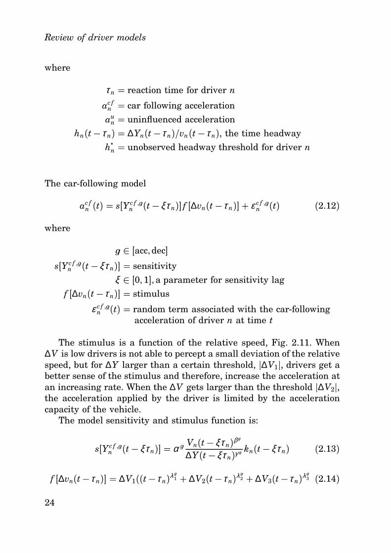
The car-following model
ac fn (t) = s[Yc f ,n
n (t − ξτ n)] f [∆vn(t −τ n)] + ε c f ,nn (t) (2.12)
where
n ∈ [acc, dec]s[Yc f ,n
n (t − ξτ n)] = sensitivity
ξ ∈ [0, 1], a parameter for sensitivity lag
f [∆vn(t −τ n)] = stimulus
ε c f ,nn (t) = random term associated with the car-following
acceleration of driver n at time t
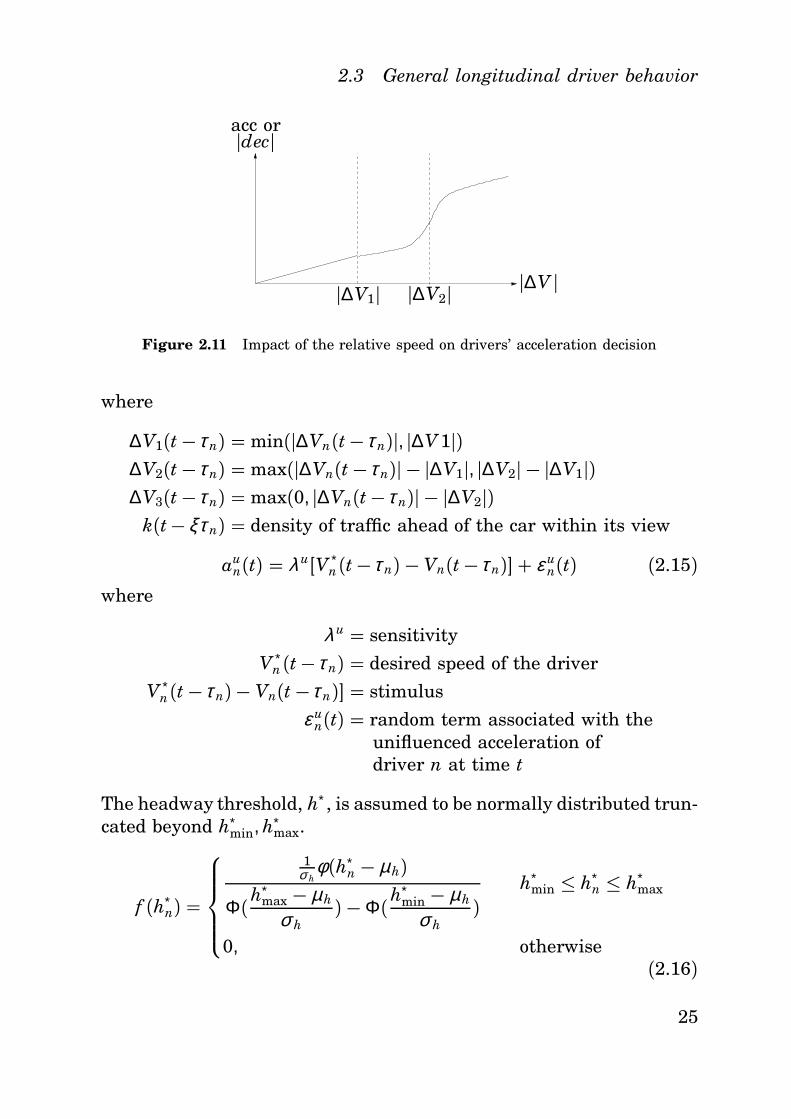
The stimulus is a function of the relative speed, Fig. 2.11. When∆V is low drivers is not able to percept a small deviation of the relativespeed, but for ∆Y larger than a certain threshold, h∆V1h, drivers get abetter sense of the stimulus and therefore, increase the acceleration atan increasing rate. When the ∆V gets larger than the threshold h∆V2h,the acceleration applied by the driver is limited by the accelerationcapacity of the vehicle.
The model sensitivity and stimulus function is:
s[Yc f ,nn (t − ξτ n)] = α n Vn(t− ξτ n)βn
∆Y(t − ξτ n)γ n kn(t− ξτ n) (2.13)
f [∆vn(t−τ n)] = ∆V1((t−τ n)λn1 + ∆V2(t−τ n)λ
n2 + ∆V3(t−τ n)λ
n3 (2.14)
24
2.3 General longitudinal driver behavior
h∆V hh∆V1h h∆V2h
acc orhdech
Figure 2.11 Impact of the relative speed on drivers’ acceleration decision
where
∆V1(t − τ n) = min(h∆Vn(t− τ n)h, h∆V 1h)∆V2(t − τ n) = max(h∆Vn(t − τ n)h − h∆V1h, h∆V2h − h∆V1h)∆V3(t − τ n) = max(0, h∆Vn(t− τ n)h − h∆V2h)
k(t− ξτ n) = density of traffic ahead of the car within its view
aun(t) = λu[V ∗
n(t− τ n) − Vn(t− τ n)] + ε un(t) (2.15)
where
λu = sensitivity
V ∗n(t− τ n) = desired speed of the driver
V ∗n(t − τ n) − Vn(t −τ n)] = stimulus
ε un(t) = random term associated with the
unifluenced acceleration ofdriver n at time t
The headway threshold, h∗, is assumed to be normally distributed trun-cated beyond h∗
min, h∗max.
f (h∗n) =
1
σ hφ(h∗
n − µh)
Φ(h∗max − µh
σ h) − Φ(h
∗min − µh
σ h)
h∗min ≤ h∗
n ≤ h∗max
0, otherwise(2.16)
25
Review of driver models
where
µ,σ = mean and standard deviation of theuntruncated distribution
h∗min, h∗
max = minimum and maximum values of h∗n
φ = probability density function
Φ = distribution function
2.4 The human driver brake behavior
Lee [35] proposed that the driver use the simplest type of visual infor-mation from the optic flow, which is sufficient for controlling braking.That is time-to-collision information (TTC) , not information about dis-tance, relative speed, or acceleration. The driver bases his judgmenton TTC information, when to start braking and to control the brakingaction. Van Der Horst [48] supported this assumption, and performeda framework which shows that both the decision when to start brakingand how to control the braking progress are based on TTC informationavailable from the optic field. In the study, it is also noticeable thata driver often brakes with a rather constant deceleration during thebrake procedure. Van Winsum and Heino [49] proposed the followinghypotheses:
• Preferred time-headway is constant over different speeds;
• Preferred time-headway is consistent within individual drivers,but differs between drivers;
• The initiation of braking, measured by brake reaction time(BRT), is more strongly related to TTC at the moment the leadvehicle starts to brake for short followers compared to long fol-lowers. This is assumed to be related to differences in the abilityto perceive TTC information;
• Preferred time-headway is related to the intensity of brakingand quality of braking control. The maximum percentage brakepressed measures the intensity of braking while the quality of
26
2.5 Safety
braking control is measured by the sensitivity of the braking in-tensity to criticality and by the time difference between tTTCmin
and tDECmax .
Usually BRT was measured as the time from the presentation of thestimulus until the foot touches the brake pedal, tTTCmin being the timewhen the minimum TTC is reached during braking, and tDECmax beingthe time when the maximum deceleration is reached during braking.
Winsum and Heino performed experiments to validate the hypothe-sis, and based on the experiments they concluded that preferred time-headway is constant over different speeds and it is consistent withinindividual drivers [49]. But there was no evidence that short follow-ers and long followers differ in sensitivity of BRT and the moment thelead vehicle starts to brake. According to the last hypothesis, preferredtime-headway is related to the intensity of braking and quality of brak-ing control, not either confirmed, but it was found that the intensityof braking is partly programmed and based on TTC.Johansson and Rumer [27] estimated the driver brake reaction timeusing data collected from 321 drivers in real traffic. By using soundas stimulus for braking and measuring the time until the brake lightturned on, they found that the brake reaction time varied from 0.4 to2.7 seconds, with a mean, and standard deviation of 1.01, and 0.37 sec-onds. Since the drivers were informed that they were participating ina brake reaction study and the use of sound as stimulus, these valuesmay be biased.
2.5 Safety
Often is it suggested that ACC will increase the safety in traffic. Themotivation for this is that the ACC give the driver assistance in thedriving tasks. The assistance will it reduce the driver’s workload, whichallows the driver to concentrate more on other tasks. This implies thatthe drivers will experience less fatigue of driving and that the drivingwill become more comfortable. The purpose of the ACC is to providesupport to the driver in a wide range of driving environments, butthe full responsibility will always be on the driver. One objection to
27
Review of driver models
that ACC increase the safety is that the driver may be over-relianton the ACC system and may not be prepared to take control of thevehicle in extreme situations. Hitz et al. [23] have done a field op-erational test in order to evaluate the safety of ACC in traffic. Thistest involved 108 drivers, which were studied for a year. In this safetystudy they use a list of standard surrogate measures of safety. Theyalso extended this to include new safety surrogates and performancemeasures. Hitz et al. compared ACC driving with manual driving andconventional cruise control (CCC) driving. In this study it was foundthat the ACC drivers tended to wait for the system to control situa-tions and therefore intervened later when necessary which led to thatbrake pressure above -0.1n where more commonly among ACC drivers,but this did not in general result in extreme situations. It also showsthat the drivers using ACC had a longer response time than humandrivers and slightly less than CCC drivers did. Since the ACC drivershave greater headway distance than manual drivers do, it is not clearthat the longer response time implies inattentiveness by the driver. Inthe study the drivers ranked the manual driving as most safe followedby ACC driving and CCC driving last. But they also agreed that ACCwould improve safety. Hitz et al. made a Monte Carlo computer simu-lation using the data from the test study in order to estimate the safetyeffects of wide spread ACC use [23]. Their simulation showed that twotypes of collisions on freeways would be reduced by 17 percent:
• Situations when an ACC equipped vehicle approaching a slowervehicle traveling at constant velocity.
• Situations when the lead vehicle decelerating in front of an ACCequipped vehicle.
The Hitz’s et al. conclusion of this field test was that if the ACC systemwould be widespread and fully implemented it would result in a net in-crease of safety. They did not propose what should be the highest valueof deceleration in an ACC system. This would require more study. To-day this deceleration authority differs among the systems available.Iijima et al. [24] found that 90 percent of all decelerations is less than2.5m/s2. In BMW’s ACC system by Prestl et al. [43], a highest decel-eration of −2m/s2 was used. Prestl et al. found this to be a suitable
28
2.6 Existing systems
compromise between customer benefit, convenience and safety. Thislow limit will ensure that the system limits are reached frequently andwill not lead the driver to become over-reliant on the system. Prestl etal. also shared Hitz et al. opinion that a new driver must learn how touse an ACC system properly and understand its limits.
Prestl et al. have chosen not to have an audible take-over alarm, thereason is that this could be misunderstood as a collision warning. Dur-ing their work, they found that a driver is very sensitive to kinestheticfeedback in the beginning of a deceleration, which will raise the driverattention. Therefore experienced drivers do not need any take-overalarm and they also have learned when to start braking. Neither Hitzet al. or Prestl et al. presented any idea how to best teach a new driverthese new requirements placed on him. Prestl et al. also presented atechnical safety concept, which includes safety in distributed systemand shutdown mechanism.
All ACC systems aim towards reducing the driver’s workload, whichwill lead to increased comfort. Nakayama et al. [40] proposed a methodof measuring the driver workload, called ”The steering entropymethod”. By measuring the driver’s variation in the steering angleduring driving, it was possible to evaluate the workload. Iijima et al.[24] used this method to conclude that their suggested ACC drivingreduced the workload in compare with CCC driving. In this study bothexperienced drivers and novice drivers participated.
2.6 Existing systems
With Navlab at Carnegie Mellon University, Thorpe et. al [47] devel-oped a Free Agent system, which fully automates driving. Their strat-egy was to surround the vehicles with sensors, putting all the sensingand decision-making in the vehicles to make them fully automated.The automated vehicles were equipped with a vision system, and aradar system. Since the most important mission for the automated ve-hicle was to increase the safety on the highways, the Free Agent wasdesigned to keep a safe space around the vehicle. The Free Agent aimsto have a large enough headway between vehicles that high-bandwidth
29
Review of driver models
throttle and brake servo are not needed. Since only low-bandwidth con-trol is needed, the existing cruise control could be used to perform allthe throttle actuation. The Free Agent was demonstrated in August1997 for the UN National Automated Highway System Consortium.During the demo several of the common actions at highways were per-formed, but not any cut-in or critical situations.
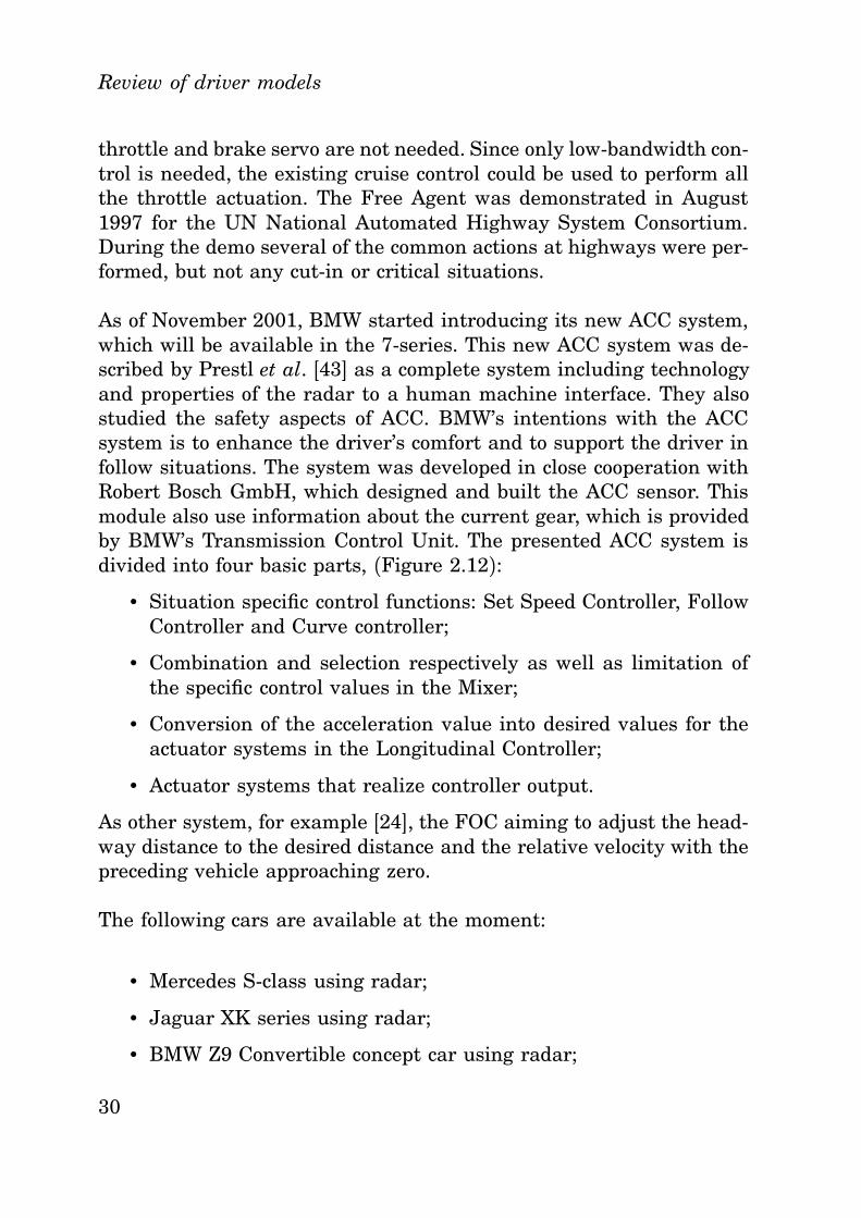
As of November 2001, BMW started introducing its new ACC system,which will be available in the 7-series. This new ACC system was de-scribed by Prestl et al. [43] as a complete system including technologyand properties of the radar to a human machine interface. They alsostudied the safety aspects of ACC. BMW’s intentions with the ACCsystem is to enhance the driver’s comfort and to support the driver infollow situations. The system was developed in close cooperation withRobert Bosch GmbH, which designed and built the ACC sensor. Thismodule also use information about the current gear, which is providedby BMW’s Transmission Control Unit. The presented ACC system isdivided into four basic parts, (Figure 2.12):
• Situation specific control functions: Set Speed Controller, FollowController and Curve controller;
• Combination and selection respectively as well as limitation ofthe specific control values in the Mixer;
• Conversion of the acceleration value into desired values for theactuator systems in the Longitudinal Controller;
• Actuator systems that realize controller output.
As other system, for example [24], the FOC aiming to adjust the head-way distance to the desired distance and the relative velocity with thepreceding vehicle approaching zero.
The following cars are available at the moment:
• Mercedes S-class using radar;
• Jaguar XK series using radar;
• BMW Z9 Convertible concept car using radar;
30

2.7 Cut in Situations
SSC
FOC
CSC
MIX LOC
Brake
Drive Train
Figure 2.12 BMW’s ACC system structure
• Toyota Celsior using laser;
• Toyota Progress using laser;
• Mitsubishi Diamante using laser;
• Lexus LS430 using laser.
2.7 Cut in Situations
In design of an ACC system aiming to increase the driver’s comfort, itis necessary understand drivers cut-in behavior. Iijma et al. [24] havestudied the behavior and included this in theirs ACC model.
2.8 Activities and WWW-links
Automated highway systems at Carnegie Mellon.http://www.cs.cmu.edu/XSGroups/ahs/
Cambridge Basic Research at laboratory of Nissan Technical CenterNorth America, Inc.http://pathfinder.cbr.com/
The Center for Advanced Transportation Technology (CATT) at theUniversity of Southern California.http://www.usc.edu/dept/ee/catt/
Vehicle Dynamics Lab (VDL)at University of California, Berkeley.http://vehicle.me.berkeley.edu/
31
Review of driver models
PATH projecthttp://www.path.berkley.edu/
The Man Vehicle Laboratory (MVL) at the Massachusetts Institute ofTechnology.http://mvl.mit.edu/
The Center for Transportation Analysis (CTA) in the Oak Ridge.http://www-cta.ornl.gov/cta/research/trb/tft.html
Intelligent Transportation Systems (ITS) at the Massachusetts Insti-tute of Technology.http://its.mit.edu/
32
3
Material & Methods
3.1 Introduction
In order to design an ACC which with the drivers feel safe and com-fortable, the ACC needs to mimic the driver behavior in traffic. Thehuman driver behavior changes in different traffic situations. There-fore, standard traffic situations have to be identified and used in theexperimental phase. Several different drivers are used to capture arange of driver behaviors.
There is a difference between carrying out experiments on publicroads and on test tracks. It is assumed that a driver’s natural behavioris best caught on public roads. If test tracks are used the subject mightshow different driver behavior. A possible reason being that the driverfeels safer on the test track and as a result drives more aggressively.
Sensors are needed to detect other vehicles in order to study hu-man driver behavior in real traffic situations. Usually the velocity anddistance to the vehicle in front are measured.
For this purpose there exist three standard sensors: the radar, thelaser, and the camera. The radar is expensive, but is robust to badweather conditions, like rain, mud, dust or snow. It offers a narrowfield-of-view of 8–12 degrees but has a long working range of around150 meters.
The laser is less expensive, but performs poorly in bad weatherbecause the laser beam is easily blocked by atmospheric particles. The
33
Material & Methods
field-of-view is easily adjustable up to 180 degrees. A typical workingrange is around 50 meters.
The camera is often used in conjunction with the radar or the laser.It is capable of easily distinguishing between moving and stationaryobjects. The field-of-view is usually large, depending on the choice oflens.
Sensor field-of-view and range parameter choices are important.For instance, a large field-of-view is advantageous when detecting cut-in vehicles, like cars switching lanes. Small field-of-view sensors, likethe radar, does not detect a vehicle until it is almost in front of thedriver’s vehicle, while a large field-of-view sensor, like the laser or acamera, detects the cut-in vehicle when it starts to switch lanes. Thechoice of appropriate range depends somewhat on the design philos-ophy behind the ACC. One opinion is that the sensor should not bebetter than a human being in order to not introduce a false sense ofsafety. Other states that the sensor should be as good as possible toenhance the capabilities of the driver driving the vehicle.
Combinations of sensors are used to achieve robust informationextraction. The combination of radar and camera uses the camera tocompensate for the small field-of-view of the radar and segment movingobjects from stationary. This may be a problem when using only range-based sensors like the radar or the laser. The laser and the camera areused in a similar manner. The combination of radar and laser can beused to increase reliability and system robustness. The sensors havedifferent fields-of-view and working range and seldom lose track of thefront vehicle at the same time. From a traffic safety point of view thisis preferable. Widmann et. al. have made a comparison of laser-basedand radar-based sensor in ACC [52].
3.2 Experimental platform
Vehicle
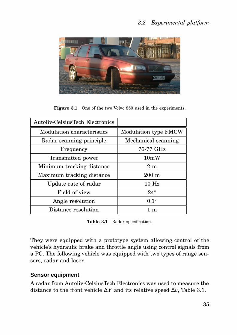
Two automatic transmission Volvo 850:s were used in a leading-vehicle-following-vehicle experimental setup (Fig. 3.1). Both vehicles havebeen used in previous ACC-projects at Volvo Technical Development.
34
3.2 Experimental platform
Figure 3.1 One of the two Volvo 850 used in the experiments.
Autoliv-CelsiusTech Electronics
Modulation characteristics Modulation type FMCW
Radar scanning principle Mechanical scanning
Frequency 76-77 GHz
Transmitted power 10mW
Minimum tracking distance 2 m
Maximum tracking distance 200 m
Update rate of radar 10 Hz
Field of view 24○
Angle resolution 0.1○
Distance resolution 1 m
Table 3.1 Radar specification.
They were equipped with a prototype system allowing control of thevehicle’s hydraulic brake and throttle angle using control signals froma PC. The following vehicle was equipped with two types of range sen-sors, radar and laser.
Sensor equipment
A radar from Autoliv-CelsiusTech Electronics was used to measure thedistance to the front vehicle ∆Y and its relative speed ∆v, Table 3.1.
35
Material & Methods
IBEO Laser scanner LD Automotive
Minimum tracking distance 0.4 m
Maximum tracking distance 100 m
Update rate of laser 10 Hz
Field of view up to 270○
Angle resolution 0.25○
Distance resolution 0.004 m
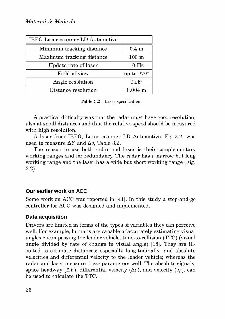
Table 3.2 Laser specification
A practical difficulty was that the radar must have good resolution,also at small distances and that the relative speed should be measuredwith high resolution.
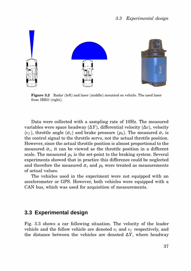
A laser from IBEO, Laser scanner LD Automotive, Fig 3.2, wasused to measure ∆Y and ∆v, Table 3.2.
The reason to use both radar and laser is their complementaryworking ranges and for redundancy. The radar has a narrow but longworking range and the laser has a wide but short working range (Fig.3.2).
Our earlier work on ACC
Some work on ACC was reported in [41]. In this study a stop-and-gocontroller for ACC was designed and implemented.
Data acquisition
Drivers are limited in terms of the types of variables they can perceivewell. For example, humans are capable of accurately estimating visualangles encompassing the leader vehicle, time-to-collision (TTC) (visualangle divided by rate of change in visual angle) [18]. They are ill-suited to estimate distances; especially longitudinally- and absolutevelocities and differential velocity to the leader vehicle; whereas theradar and laser measure these parameters well. The absolute signals,space headway (∆Y), differential velocity (∆v), and velocity (vf ), canbe used to calculate the TTC.
36
3.3 Experimental design
Figure 3.2 Radar (left) and laser (middle) mounted on vehicle. The used laserfrom IBEO (right).
Data were collected with a sampling rate of 10Hz. The measuredvariables were space headway (∆Y), differential velocity (∆v), velocity(vf ), throttle angle (α t) and brake pressure (pb). The measured α t isthe control signal to the throttle servo, not the actual throttle position.However, since the actual throttle position is almost proportional to themeasured α t, it can be viewed as the throttle position in a differentscale. The measured pb is the set-point to the braking system. Severalexperiments showed that in practice this difference could be neglectedand therefore the measured α t and pb were treated as measurementsof actual values.
The vehicles used in the experiment were not equipped with anaccelerometer or GPS. However, both vehicles were equipped with aCAN bus, which was used for acquisition of measurements.
3.3 Experimental design
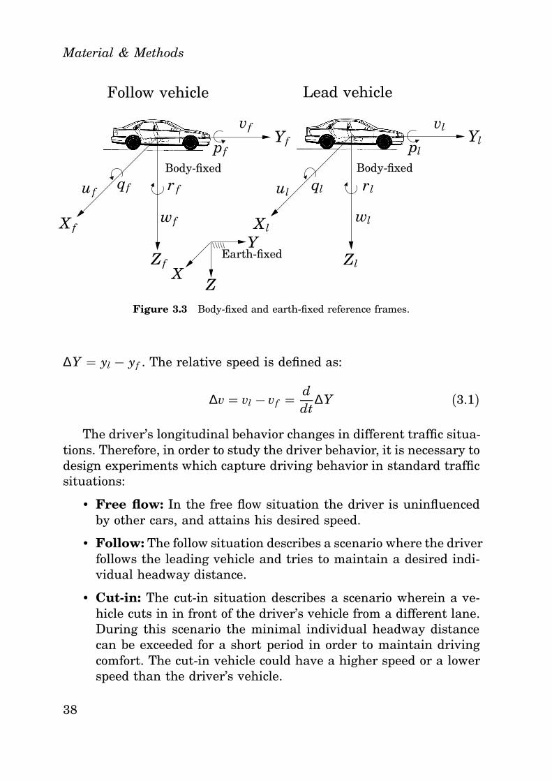
Fig. 3.3 shows a car following situation. The velocity of the leadervehicle and the follow vehicle are denoted vl and vf respectively, andthe distance between the vehicles are denoted ∆Y , where headway
37
Material & Methods
vf vlYf
X f
Zf
uf ul
wf wl
r f rl
pf pl
qf ql
Yl
Xl
Zl
Y
XZ
Lead vehicle
Body-fixedBody-fixed
Earth-fixed
Follow vehicle
Figure 3.3 Body-fixed and earth-fixed reference frames.
∆Y = yl − yf . The relative speed is defined as:
∆v = vl − vf = ddt
∆Y (3.1)
The driver’s longitudinal behavior changes in different traffic situa-tions. Therefore, in order to study the driver behavior, it is necessary todesign experiments which capture driving behavior in standard trafficsituations:
• Free flow: In the free flow situation the driver is uninfluencedby other cars, and attains his desired speed.
• Follow: The follow situation describes a scenario where the driverfollows the leading vehicle and tries to maintain a desired indi-vidual headway distance.
• Cut-in: The cut-in situation describes a scenario wherein a ve-hicle cuts in in front of the driver’s vehicle from a different lane.During this scenario the minimal individual headway distancecan be exceeded for a short period in order to maintain drivingcomfort. The cut-in vehicle could have a higher speed or a lowerspeed than the driver’s vehicle.
38
3.3 Experimental design
• Braking: In a braking situation, the headway distance decreasesbelow the individual minimal headway distance, and the driverbrakes to reestablish the headway distance.
• Approaching: In an approaching situation the driver is closingup behind the front vehicle and starts to adjust his speed to thevehicle in front. During this situation the driver change from freeflow driving to car following.
Follow situations
The Follow situation data were collected for 8 different experiments,performed on public roads as well as on a test track. Six of theseexperiments were performed on two lane public roads and the velocitywas in the range of 65 to 90 km/h. The experiments were designed tomimic free way and main country road environments. The velocity ofthe leader vehicle changes smoothly, without fast accelerations. Twoof these experiments were performed on a two-lane test track andthe velocity was in the range of 0 to 55 km/h. The experiments weredesigned to mimic urban environment and included some stop-and-gosituations. The velocity of the leader vehicle in urban situations canchange fast which was taken into account during the design of theexperiments.
As well known, human drivers differ in their behavior, each driverhaving his own driving behavior, different desired headway distance,more or less aggressive, etc. To study the driving behavior it is de-sirable to be able to repeat exactly the same experiment for each testperson who participated in the study. This was achieved since the usedleading vehicle in the study was equipped with a system allowing con-trol of the brakes and of the throttle. The experiment was then per-formed in the following way.
• The kind of situation was decided (country side/urban).• The road and length of the experiment were chosen.
• The vehicle which was used as the leader vehicle in the experi-ment was used to drive the chosen road part and the brake pres-sure and throttle angle were measured and stored.
The leader vehicle had the property of being programmable to drivealong a predefined longitudinal trajectory, which was specified using
39
Material & Methods
0 50 100 150 200 250 300 350 40060
70
80
90
100
v l[k
m/h]
Time [s]
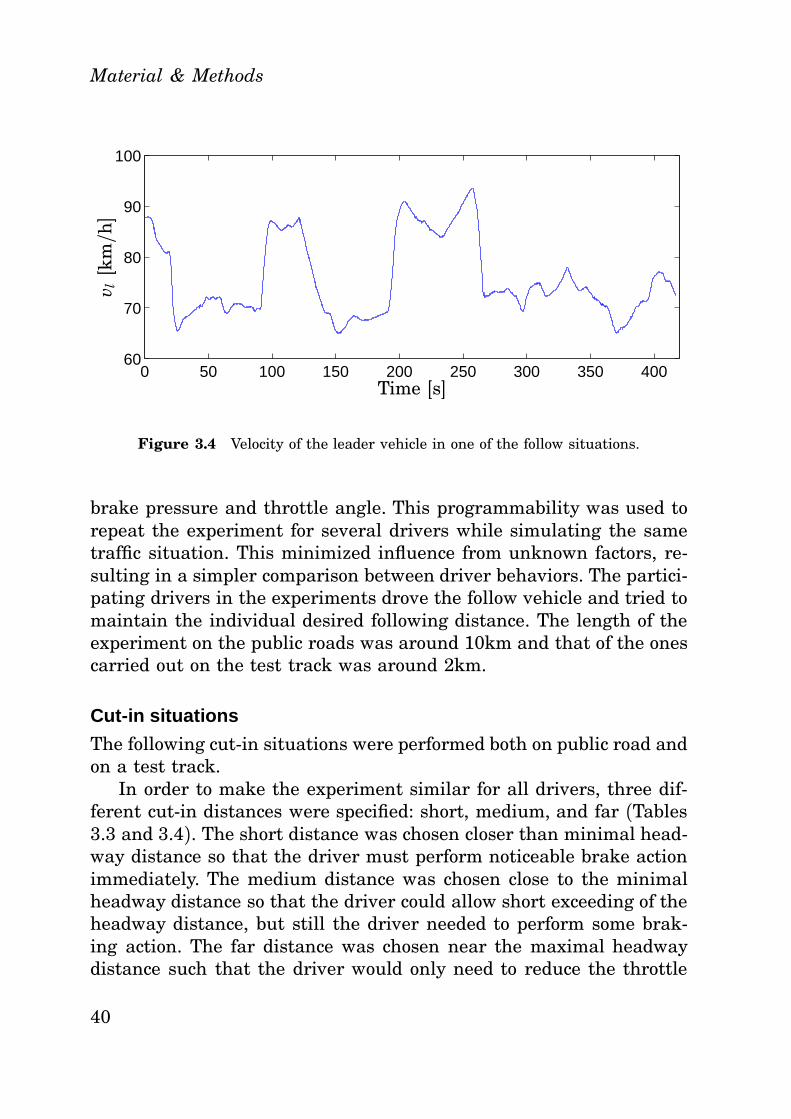
Figure 3.4 Velocity of the leader vehicle in one of the follow situations.
brake pressure and throttle angle. This programmability was used torepeat the experiment for several drivers while simulating the sametraffic situation. This minimized influence from unknown factors, re-sulting in a simpler comparison between driver behaviors. The partici-pating drivers in the experiments drove the follow vehicle and tried tomaintain the individual desired following distance. The length of theexperiment on the public roads was around 10km and that of the onescarried out on the test track was around 2km.
Cut-in situations
The following cut-in situations were performed both on public road andon a test track.
In order to make the experiment similar for all drivers, three dif-ferent cut-in distances were specified: short, medium, and far (Tables3.3 and 3.4). The short distance was chosen closer than minimal head-way distance so that the driver must perform noticeable brake actionimmediately. The medium distance was chosen close to the minimalheadway distance so that the driver could allow short exceeding of theheadway distance, but still the driver needed to perform some brak-ing action. The far distance was chosen near the maximal headwaydistance such that the driver would only need to reduce the throttle
40

3.3 Experimental design
Vleader (km/h) Vf ollower (km/h) ∆distance (m)40 50 short
40 50 medium
40 50 far
50 50 short
50 50 medium
50 50 far
60 50 short
60 50 medium
60 50 far
60 70 short
60 70 medium
60 70 far
70 70 short
70 70 medium
70 70 far
80 70 short
80 70 medium
80 70 far
80 90 short
80 90 medium
80 90 far
90 90 short
90 90 medium
90 90 far
100 90 short
100 90 medium
100 90 far
Table 3.3 Experimental protocol of cut-in situations.
41
Material & Methods
Vleader (km/h) Vf ollower (km/h) ∆distance (m)90 110 short
90 110 medium
90 110 far
100 110 short
100 110 medium
100 110 far
110 110 short
110 110 medium
110 110 far
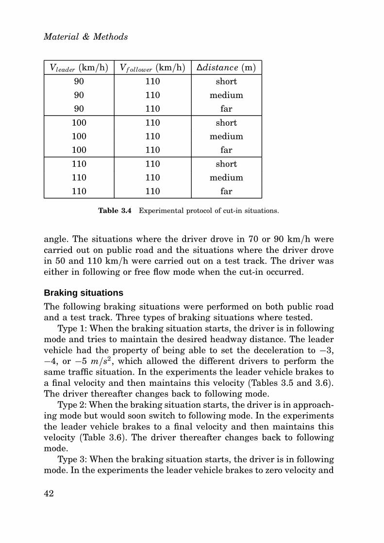
Table 3.4 Experimental protocol of cut-in situations.
angle. The situations where the driver drove in 70 or 90 km/h werecarried out on public road and the situations where the driver drovein 50 and 110 km/h were carried out on a test track. The driver waseither in following or free flow mode when the cut-in occurred.
Braking situations
The following braking situations were performed on both public roadand a test track. Three types of braking situations where tested.
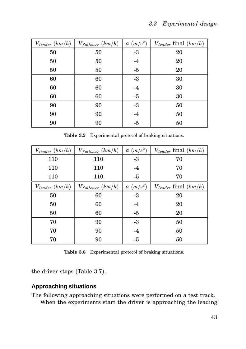
Type 1: When the braking situation starts, the driver is in followingmode and tries to maintain the desired headway distance. The leadervehicle had the property of being able to set the deceleration to −3,−4, or −5 m/s2, which allowed the different drivers to perform thesame traffic situation. In the experiments the leader vehicle brakes toa final velocity and then maintains this velocity (Tables 3.5 and 3.6).The driver thereafter changes back to following mode.
Type 2: When the braking situation starts, the driver is in approach-ing mode but would soon switch to following mode. In the experimentsthe leader vehicle brakes to a final velocity and then maintains thisvelocity (Table 3.6). The driver thereafter changes back to followingmode.
Type 3: When the braking situation starts, the driver is in followingmode. In the experiments the leader vehicle brakes to zero velocity and
42
3.3 Experimental design
Vleader (km/h) Vf ollower (km/h) a (m/s2) Vleader final (km/h)50 50 -3 20
50 50 -4 20
50 50 -5 20
60 60 -3 30
60 60 -4 30
60 60 -5 30
90 90 -3 50
90 90 -4 50
90 90 -5 50
Table 3.5 Experimental protocol of braking situations.
Vleader (km/h) Vf ollower (km/h) a (m/s2) Vleader final (km/h)110 110 -3 70
110 110 -4 70
110 110 -5 70
Vleader (km/h) Vf ollower (km/h) a (m/s2) Vleader final (km/h)50 60 -3 20
50 60 -4 20
50 60 -5 20
70 90 -3 50
70 90 -4 50
70 90 -5 50
Table 3.6 Experimental protocol of braking situations.
the driver stops (Table 3.7).
Approaching situations
The following approaching situations were performed on a test track.When the experiments start the driver is approaching the leading
43
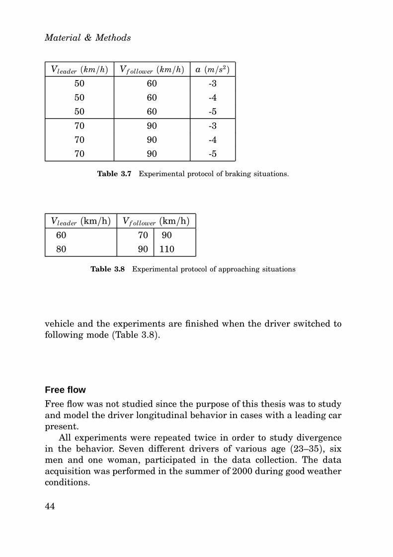
Material & Methods
Vleader (km/h) Vf ollower (km/h) a (m/s2)50 60 -3
50 60 -4
50 60 -5
70 90 -3
70 90 -4
70 90 -5
Table 3.7 Experimental protocol of braking situations.
Vleader (km/h) Vf ollower (km/h)60
80
70 90
90 110
Table 3.8 Experimental protocol of approaching situations
vehicle and the experiments are finished when the driver switched tofollowing mode (Table 3.8).
Free flow
Free flow was not studied since the purpose of this thesis was to studyand model the driver longitudinal behavior in cases with a leading carpresent.
All experiments were repeated twice in order to study divergencein the behavior. Seven different drivers of various age (23–35), sixmen and one woman, participated in the data collection. The dataacquisition was performed in the summer of 2000 during good weatherconditions.
44
3.4 System identification
vf
∆Y
∆vpb
α t
System 1
Driver vl vf
∆Y
∆v
pb
α t
System 2
Driver
Figure 3.5 Representations of two different input and output separations.System 1 is the standard separation.
3.4 System identification
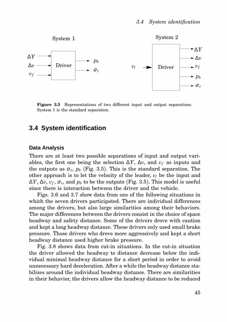
Data Analysis
There are at least two possible separations of input and output vari-ables, the first one being the selection ∆Y , ∆v, and vf as inputs andthe outputs as α t, pb (Fig. 3.5). This is the standard separation. Theother approach is to let the velocity of the leader, vl be the input and∆Y , ∆v, vf , α t, and pb to be the outputs (Fig. 3.5). This model is usefulsince there is interaction between the driver and the vehicle.
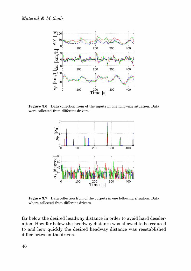
Figs. 3.6 and 3.7 show data from one of the following situations inwhich the seven drivers participated. There are individual differencesamong the drivers, but also large similarities among their behaviors.The major differences between the drivers consist in the choice of spaceheadway and safety distance. Some of the drivers drove with cautionand kept a long headway distance. These drivers only used small brakepressure. Those drivers who drove more aggressively and kept a shortheadway distance used higher brake pressure.
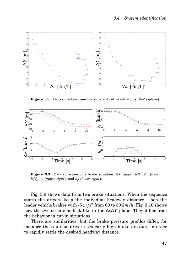
Fig. 3.8 shows data from cut-in situations. In the cut-in situationthe driver allowed the headway to distance decrease below the indi-vidual minimal headway distance for a short period in order to avoidunnecessary hard deceleration. After a while the headway distance sta-bilizes around the individual headway distance. There are similaritiesin their behavior, the drivers allow the headway distance to be reduced
45
Material & Methods
0 100 200 300 4000
50
100
0 100 200 300 400−5
0
5
0 100 200 300 400
50
100
v f[k
m/h]
∆Y[m]
∆v[k
m/h]
Time [s]
Figure 3.6 Data collection from of the inputs in one following situation. Datawere collected from different drivers.
0 100 200 300 4000
1
2
0 100 200 300 4000
20
40
60
80
Time [s]
p b[P
a]α
t[d
egre
e]
Figure 3.7 Data collection from of the outputs in one following situation. Datawhere collected from different drivers.
far below the desired headway distance in order to avoid hard deceler-ation. How far below the headway distance was allowed to be reducedto and how quickly the desired headway distance was reestablisheddiffer between the drivers.
46
3.4 System identification
−6 −5 −4 −3 −2 −1 0 1 219
20
21
22
23
24
25
26
27
28
∆Y[m]
∆v [km/h] −4 −3 −2 −1 0 1 235
36
37
38
39
40
41
42
43
44
45
∆Y[m]
∆v [km/h]
Figure 3.8 Data collection from two different cut in situations (∆v∆ y-plane).
0 2 4 6 8 1010
20
30
40
50
0 2 4 6 8 10 12−10
−5
0
5
Time [s]
∆Y[m]
∆v[k
m/h]
0 2 4 6 8 1020
40
60
0 2 4 6 8 10 120
1
2
3
Time [s]
v f[k
m/h]
b p[P
a]
Figure 3.9 Data collection of a brake situation. ∆Y (upper left), ∆v (lowerleft), vf (upper right), and bp (lower right).
Fig. 3.9 shows data from two brake situations. When the sequencestarts the drivers keep the individual headway distance. Then theleader vehicle brakes with -5 m/s2 from 60 to 30 km/h. Fig. 3.10 showshow the two situations look like in the ∆v∆Y-plane. They differ fromthe behavior in cut-in situations.
There are similarities, but the brake pressure profiles differ, forinstance the cautious driver uses early high brake pressure in orderto rapidly settle the desired headway distance.
47
Material & Methods
−3 −2.5 −2 −1.5 −1 −0.5 0 0.51
1.5
2
2.5
3
3.5
4
−3.5 −3 −2.5 −2 −1.5 −1 −0.5 0 0.51.5
2
2.5
3
3.5
4
4.5
Figure 3.10 Data collection from two different braking situations (∆v∆Y-plane).
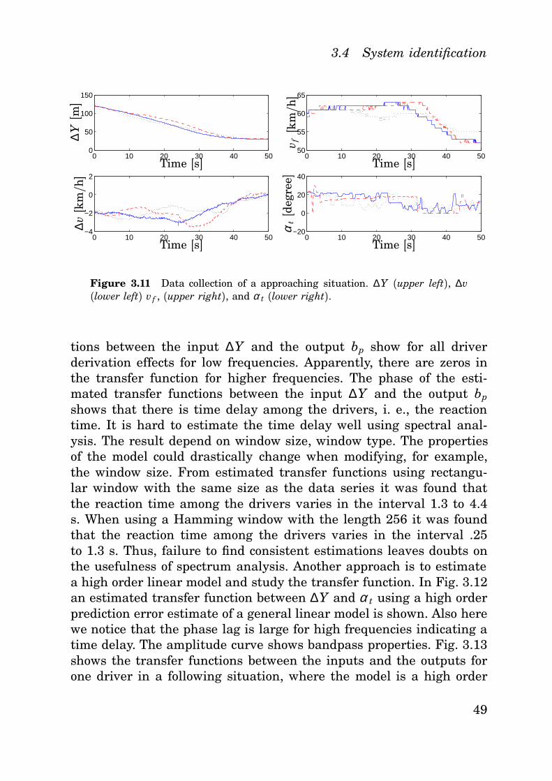
Fig. 3.11 shows data from an approaching situation where thedriver changed his behavior from free flow mode to following mode.When the situation started the driver drove in free flow mode andthen caught up with a leader vehicle and started to adjust his speedto the vehicle in front. In the end of the sequence the driver tried tomaintain his desired headway distance. Different drivers start to ad-just the velocity to the vehicle in front at different moments. Somestart early to adjust the speed and uses a long time to catch up withthe vehicle and to switch to following mode, others start later and useshorter time to catch up.
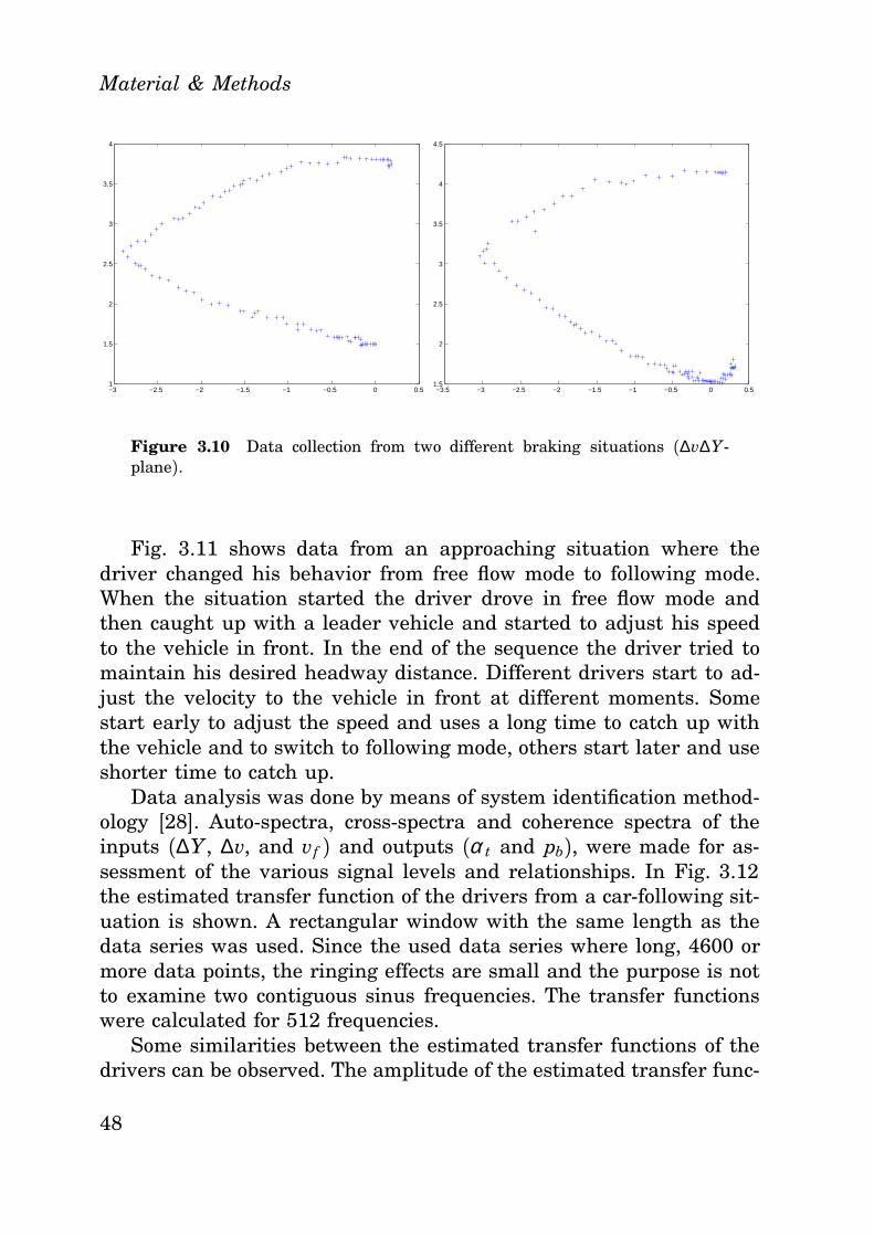
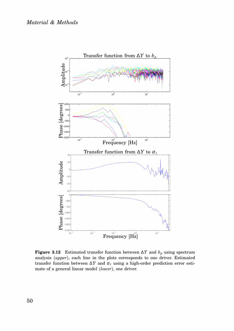
Data analysis was done by means of system identification method-ology [28]. Auto-spectra, cross-spectra and coherence spectra of theinputs (∆Y , ∆v, and vf ) and outputs (α t and pb), were made for as-sessment of the various signal levels and relationships. In Fig. 3.12the estimated transfer function of the drivers from a car-following sit-uation is shown. A rectangular window with the same length as thedata series was used. Since the used data series where long, 4600 ormore data points, the ringing effects are small and the purpose is notto examine two contiguous sinus frequencies. The transfer functionswere calculated for 512 frequencies.
Some similarities between the estimated transfer functions of thedrivers can be observed. The amplitude of the estimated transfer func-
48
3.4 System identification
0 10 20 30 40 500
50
100
150
0 10 20 30 40 50−4
−2
0
2
Time [s]
Time [s]
∆Y[m]
∆v[k
m/h]
0 10 20 30 40 5050
55
60
65
0 10 20 30 40 50−20
0
20
40
Time [s]
Time [s]
v f[k
m/h]
αt[d
egre
e]Figure 3.11 Data collection of a approaching situation. ∆Y (upper left), ∆v(lower left) vf , (upper right), and α t (lower right).
tions between the input ∆Y and the output bp show for all driverderivation effects for low frequencies. Apparently, there are zeros inthe transfer function for higher frequencies. The phase of the esti-mated transfer functions between the input ∆Y and the output bp
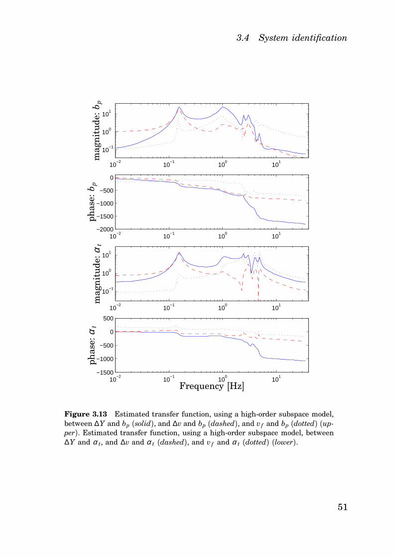
shows that there is time delay among the drivers, i. e., the reactiontime. It is hard to estimate the time delay well using spectral anal-ysis. The result depend on window size, window type. The propertiesof the model could drastically change when modifying, for example,the window size. From estimated transfer functions using rectangu-lar window with the same size as the data series it was found thatthe reaction time among the drivers varies in the interval 1.3 to 4.4s. When using a Hamming window with the length 256 it was foundthat the reaction time among the drivers varies in the interval .25to 1.3 s. Thus, failure to find consistent estimations leaves doubts onthe usefulness of spectrum analysis. Another approach is to estimatea high order linear model and study the transfer function. In Fig. 3.12an estimated transfer function between ∆Y and α t using a high orderprediction error estimate of a general linear model is shown. Also herewe notice that the phase lag is large for high frequencies indicating atime delay. The amplitude curve shows bandpass properties. Fig. 3.13shows the transfer functions between the inputs and the outputs forone driver in a following situation, where the model is a high order
49
Material & Methods
10−1
100
101
10−4
10−2
100
10−1
100
101
−2000
−1500
−1000
−500
0
500
1000
Am
plit
ude
Pha
se[d
egre
es]
Transfer function from ∆Y to bp
Frequency [Hz]
−60
−40
−20
0
20
40
10−3
10−2
10−1
100
101
−2160
−1800
−1440
−1080
−720
−360
0
Pha
se[d
egre
es]
Am
plit
ude
Frequency [Hz]
Transfer function from ∆Y to α t
Figure 3.12 Estimated transfer function between ∆Y and bp using spectrumanalysis (upper), each line in the plots corresponds to one driver. Estimatedtransfer function between ∆Y and α t using a high-order prediction error esti-mate of a general linear model (lower), one driver.
50
3.4 System identification
10−2
10−1
100
101
10−1
100
101
10−2
10−1
100
101
−2000
−1500
−1000
−500
0
10−2
10−1
100
101
10−1
100
101
10−2
10−1
100
101
−1500
−1000
−500
0
500
mag
nit
ude
:b p
phas
e:b p
mag
nit
ude
:αt
phas
e:α
t
Frequency [Hz]
Figure 3.13 Estimated transfer function, using a high-order subspace model,between ∆Y and bp (solid), and ∆v and bp (dashed), and vf and bp (dotted) (up-per). Estimated transfer function, using a high-order subspace model, between∆Y and α t, and ∆v and α t (dashed), and vf and α t (dotted) (lower).
51
Material & Methods
10−1
100
101
0
0.5
1
10−1
100
101
0
0.5
1
p b[P
a]α
t[d
egre
e]
Frequency [Hz]
Frequency [Hz]
Figure 3.14 Coherence spectra between the inputs and the outputs. The upperfigure: coherence between inputs [∆Y ∆v vf ] and the output pb. The lowerfigure: coherence between inputs [∆Y ∆v vf ] and the output α t.
state space model estimated using the subspace method. The driverproves to have bandpass properties and this is also what we wouldexpect, since it has been found elsewhere that human sensors havebandpass properties [9].
Drivers use the throttle in a different manner than the brakes.The throttle is almost continuously used and often the changes areslow. The brakes are seldom used and changes can be fast or slow.The reaction time is best estimated using braking situations. Driversplan the usage of the throttle using the assumption that if no obstacleis seen the leader vehicle will keep the current velocity. This couldexplain some of the differences between the bp and the α t.
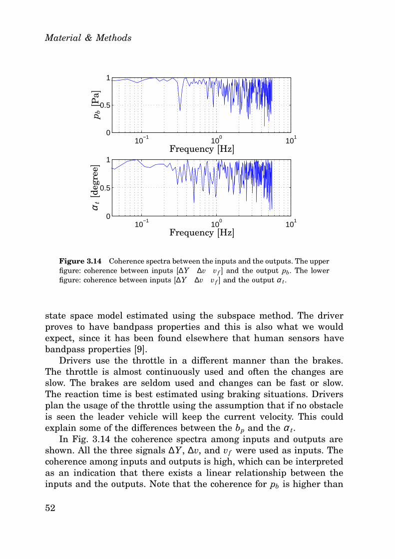
In Fig. 3.14 the coherence spectra among inputs and outputs areshown. All the three signals ∆Y , ∆v, and vf were used as inputs. Thecoherence among inputs and outputs is high, which can be interpretedas an indication that there exists a linear relationship between theinputs and the outputs. Note that the coherence for pb is higher than
52
3.4 System identification
yHumandriver
Vehicledynamics
wv
rpb
α t
Figure 3.15 Structure of a human driver in car-following with r as the inputsto the driver from the lead vehicle, v as the observation noise, w as the motornoise, and y as the car position and velocity.
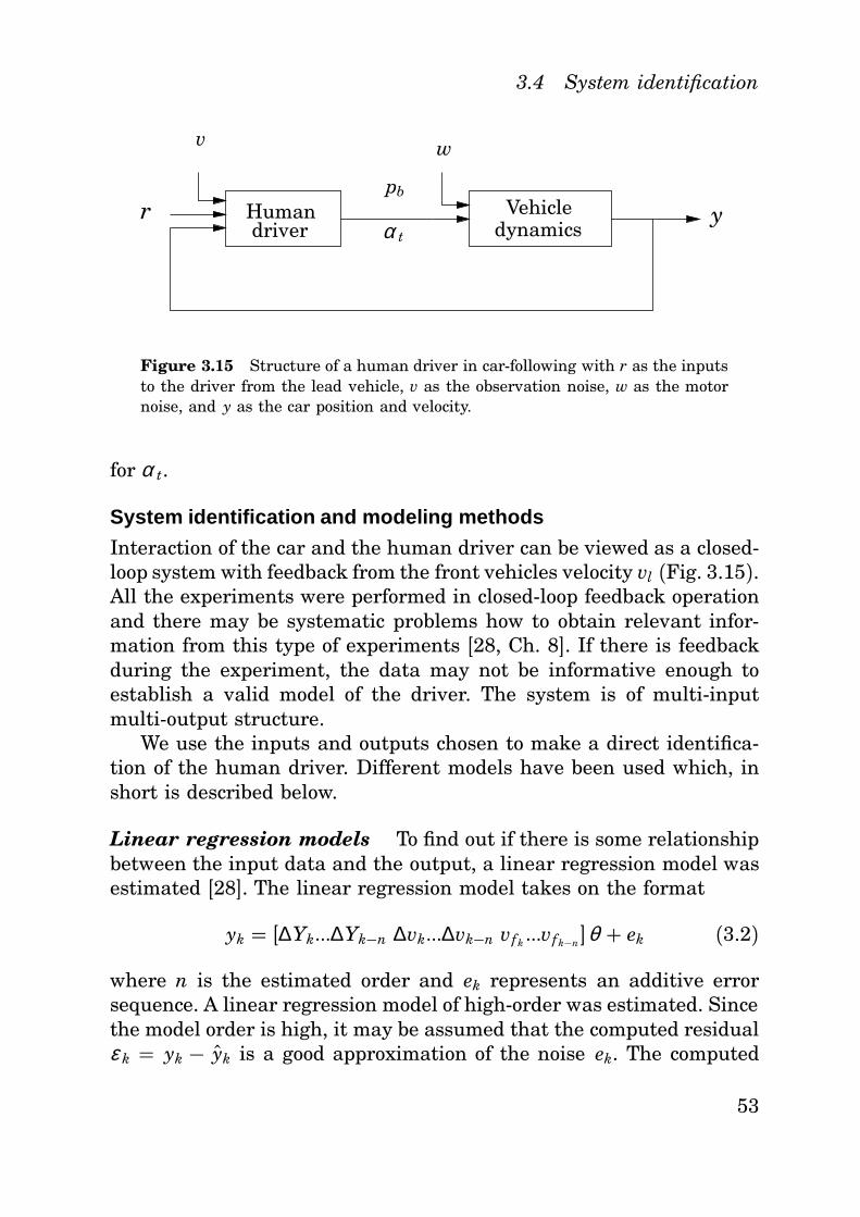
for α t.
System identification and modeling methods
Interaction of the car and the human driver can be viewed as a closed-loop system with feedback from the front vehicles velocity vl (Fig. 3.15).All the experiments were performed in closed-loop feedback operationand there may be systematic problems how to obtain relevant infor-mation from this type of experiments [28, Ch. 8]. If there is feedbackduring the experiment, the data may not be informative enough toestablish a valid model of the driver. The system is of multi-inputmulti-output structure.
We use the inputs and outputs chosen to make a direct identifica-tion of the human driver. Different models have been used which, inshort is described below.
Linear regression models To find out if there is some relationshipbetween the input data and the output, a linear regression model wasestimated [28]. The linear regression model takes on the format
yk = [∆Yk...∆Yk−n ∆vk...∆vk−n vfk ...vfk−n]θ + ek (3.2)
where n is the estimated order and ek represents an additive errorsequence. A linear regression model of high-order was estimated. Sincethe model order is high, it may be assumed that the computed residualε k = yk − yk is a good approximation of the noise ek. The computed
53
Material & Methods
residual sequence was used in pseudolinear regression to estimate amodel of lower order. This method is also known as a two-step linearregression approach.
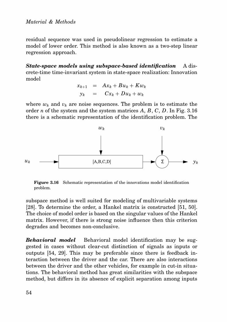
State-space models using subspace-based identification A dis-crete-time time-invariant system in state-space realization: Innovationmodel
xk+1 = Axk + Buk + Kwk
yk = Cxk + Duk+ wk
where wk and vk are noise sequences. The problem is to estimate theorder n of the system and the system matrices A, B, C, D. In Fig. 3.16there is a schematic representation of the identification problem. The
[A,B,C,D]
vkwk
ykuk Σ
Figure 3.16 Schematic representation of the innovations model identificationproblem.
subspace method is well suited for modeling of multivariable systems[28]. To determine the order, a Hankel matrix is constructed [51, 50].The choice of model order is based on the singular values of the Hankelmatrix. However, if there is strong noise influence then this criteriondegrades and becomes non-conclusive.
Behavioral model Behavioral model identification may be sug-gested in cases without clear-cut distinction of signals as inputs oroutputs [54, 29]. This may be preferable since there is feedback in-teraction between the driver and the car. There are also interactionsbetween the driver and the other vehicles, for example in cut-in situa-tions. The behavioral method has great similarities with the subspacemethod, but differs in its absence of explicit separation among inputs
54
3.4 System identification
and outputs. Thus, the estimated state-space model represents all thedynamics, both for the inputs and for the outputs. Then by matrixfraction description an input-output model can be obtained.
Detection of changed driver behavior The driver behavior de-pends on the traffic situation, it is therefore interesting to be able todetect changes in the behavior. One way to do this is to use a Gener-alized Auto-Regressive Conditional Heteroscedasticity, GARCH(r,m)model [8, 21].
An AR process of an order k is described as:
A(z−1)yk = ek (3.3)
where ek is white noise:
E{ek} = 0 (3.4)
E{ekei} ={
σ 2, k = i
0, otherwise(3.5)
The model could be used to predict the output yk. Sometimes it isinteresting not only to predict the output yk, but also its variance. Het-eroscedasticity refers to unequal variance in the regression errors, thevariance changes over time. One approach is to model the amplitudevarying residuals u2
k as an AR(m) process:
u2k = ζ +α 1u2
k−1 +α 2u2k−2 + ⋅ ⋅ ⋅+α mu2
k−m + wk (3.6)
where wk is a new white noise sequence:
E{wk} = 0 (3.7)
E{wkwi} ={
λ2, k = i
0, otherwise(3.8)
A process uk satisfying 3.6 is called an autoregressive conditional het-eroskedasticity (ARCH) process. An alternative representation is:
uk =√
hkvk (3.9)
55
Material & Methods
where vk is white noise:
E{vk} = 0 E{v2k} = 1 (3.10)
andhk = ζ +α 1u2
k−1 +α 2u2k−2 + ⋅ ⋅ ⋅+α mu2
k−m (3.11)The ACRH model can be extended into a generalized autoregressive
conditional heteroskedasticity (GARCH) model which also includeslags of u2
k.
hk = κ +δ 1hk−1+δ 2hk−2+ ⋅ ⋅ ⋅+δ rhk−r+α 1u2k−1+α 2u2
k−2+ ⋅ ⋅ ⋅+α mu2k−m
(3.12)for
κ � [1− δ 1 + δ 2 + ⋅ ⋅ ⋅+ δ r] (3.13)This could be used to model the behavior when the driver changesbehavior in a traffic situation or due to the leader vehicle brakes ora vehicle cuts in when driving in following mode. Then the residualfor a model designed for following mode becomes large, i.e., the driverdiverge from following behavior.
3.5 Transposed data
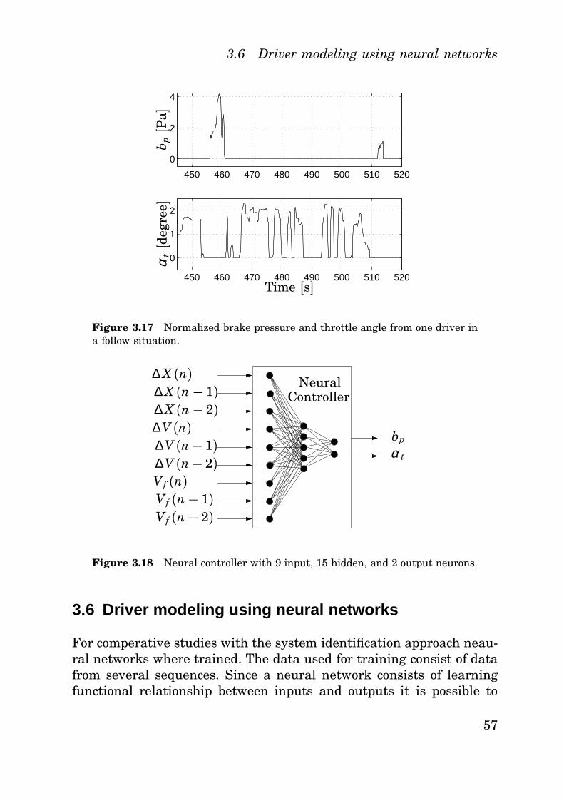
Human drivers are difficult to model by linear models in their use ofbrakes and throttle. The throttle angle and the brake pressure arenever less than zero and they are only piecewise active (Fig. 3.17).Using this fact, the result from the linear methods can be improvedby transposing the resulting negative brake pressure to positive throt-tle angle and negative throttle angle to positive brake pressure. Thetransposed data is achieved by the following procedure:
• Estimate a model using normalized data;
• Simulate the estimated model;
• Truncate the data at zero level and move negative bp to positiveα t and negative α t to positive bp.
Then the new transposed data provide acceleration-deceleration data,taking only positive values.. This is an attempt to improve the accuracyof the estimated models, and it proved to increase the result.
56
3.6 Driver modeling using neural networks
450 460 470 480 490 500 510 520
0
2
4
450 460 470 480 490 500 510 520
0
1
2
Time [s]
b p[P
a]α
t[d
egre
e]
Figure 3.17 Normalized brake pressure and throttle angle from one driver ina follow situation.
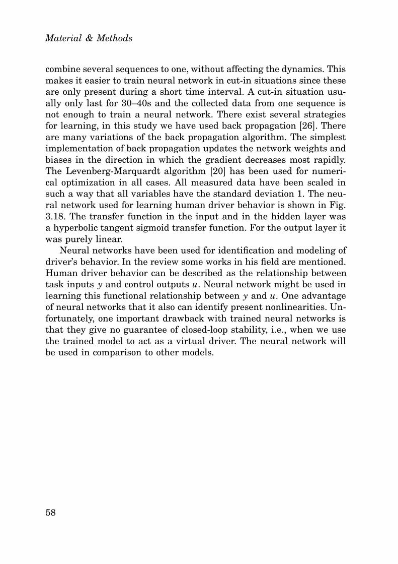
∆ X (n)∆ X (n − 1)∆ X (n − 2)∆V (n)∆V (n− 1)∆V (n− 2)Vf (n)Vf (n − 1)Vf (n − 2)
bp
α t
NeuralController
Figure 3.18 Neural controller with 9 input, 15 hidden, and 2 output neurons.
3.6 Driver modeling using neural networks
For comperative studies with the system identification approach neau-ral networks where trained. The data used for training consist of datafrom several sequences. Since a neural network consists of learningfunctional relationship between inputs and outputs it is possible to
57
Material & Methods
combine several sequences to one, without affecting the dynamics. Thismakes it easier to train neural network in cut-in situations since theseare only present during a short time interval. A cut-in situation usu-ally only last for 30–40s and the collected data from one sequence isnot enough to train a neural network. There exist several strategiesfor learning, in this study we have used back propagation [26]. Thereare many variations of the back propagation algorithm. The simplestimplementation of back propagation updates the network weights andbiases in the direction in which the gradient decreases most rapidly.The Levenberg-Marquardt algorithm [20] has been used for numeri-cal optimization in all cases. All measured data have been scaled insuch a way that all variables have the standard deviation 1. The neu-ral network used for learning human driver behavior is shown in Fig.3.18. The transfer function in the input and in the hidden layer wasa hyperbolic tangent sigmoid transfer function. For the output layer itwas purely linear.
Neural networks have been used for identification and modeling ofdriver’s behavior. In the review some works in his field are mentioned.Human driver behavior can be described as the relationship betweentask inputs y and control outputs u. Neural network might be used inlearning this functional relationship between y and u. One advantageof neural networks that it also can identify present nonlinearities. Un-fortunately, one important drawback with trained neural networks isthat they give no guarantee of closed-loop stability, i.e., when we usethe trained model to act as a virtual driver. The neural network willbe used in comparison to other models.
58
4
Validation & Results
4.1 Introduction
Different model structures have been designed and validated. The es-timated models have been simulated in Matlab and in Simulink. Inorder to study the usefulness of different identification methods forthe capturing of human driver behavior, a follow, a cut-in, and a brak-ing situation were chosen and were used as test cases for all methods.
The follow situation involves two braking sequences, one larger andone smaller. The leader vehicle also made the driver to use the throt-tle actively during this sequence. The data is from one of the followsituation and the total length of the situation is around 7 minutes. Inthe estimation of the model all 7 minutes of data were used.
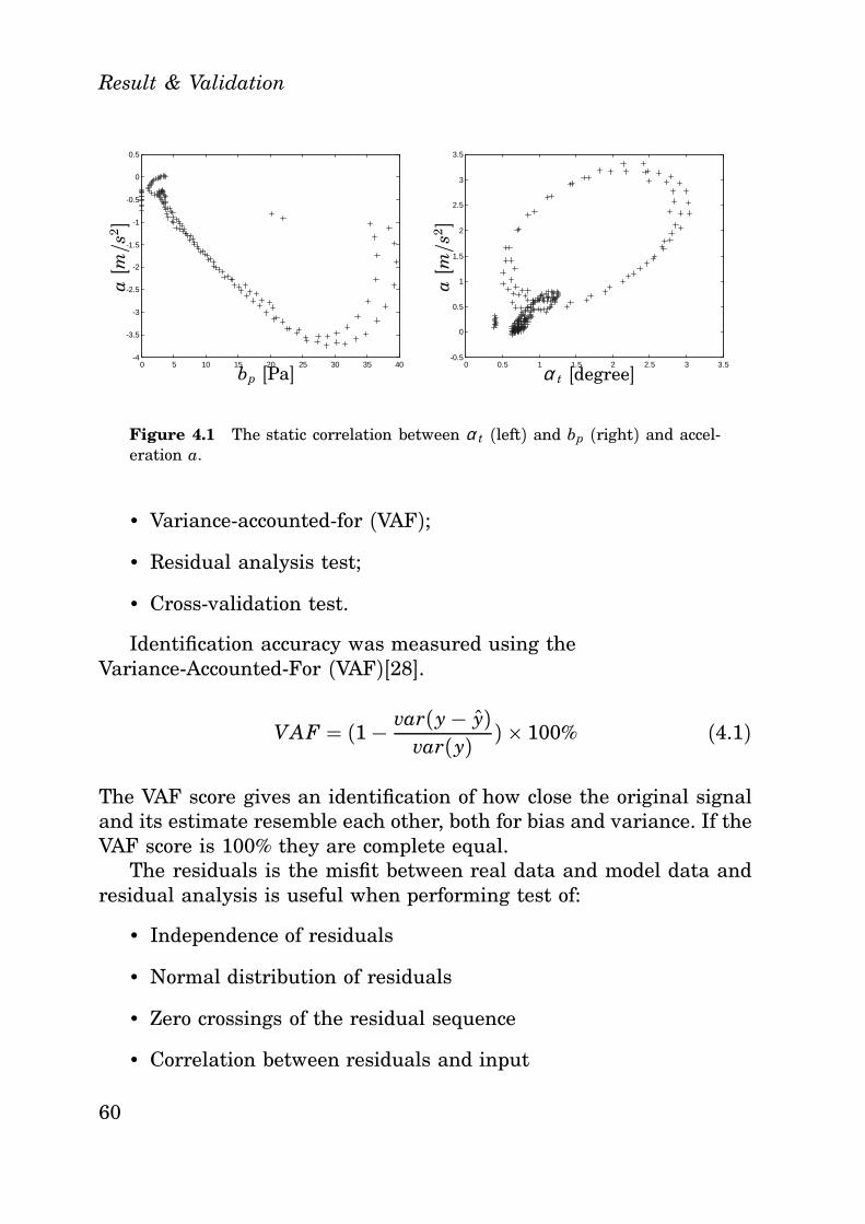
By studying the correlation between α t and acceleration, and be-tween bp and acceleration it was found that the brake and the throttlehave different dynamic properties (Fig. 4.1). This is due to the fact thatbrake pressure affects the wheel almost directly, whereas the throttleonly affects the carburetor air stream, which affects the combustionengine, which affects the transmission system, which finally affectsthe wheel.
Model validation was perfromed to verify whether the identifiedmodel fulfills the requirements of good model approximation proper-ties. Methods used in the validation process were:
59
Result & Validation
0 5 10 15 20 25 30 35 40-4
-3.5
-3
-2.5
-2
-1.5
-1
-0.5
0
0.5
0 0.5 1 1.5 2 2.5 3 3.5-0.5
0
0.5
1
1.5
2
2.5
3
3.5
α t [degree]bp [Pa]
a[m/s
2]
a[m/s
2]
Figure 4.1 The static correlation between α t (left) and bp (right) and accel-eration a.
• Variance-accounted-for (VAF);• Residual analysis test;
• Cross-validation test.
Identification accuracy was measured using theVariance-Accounted-For (VAF)[28].
VAF = (1 − var(y− y)var(y) ) � 100% (4.1)
The VAF score gives an identification of how close the original signaland its estimate resemble each other, both for bias and variance. If theVAF score is 100% they are complete equal.
The residuals is the misfit between real data and model data andresidual analysis is useful when performing test of:
• Independence of residuals
• Normal distribution of residuals
• Zero crossings of the residual sequence
• Correlation between residuals and input
60
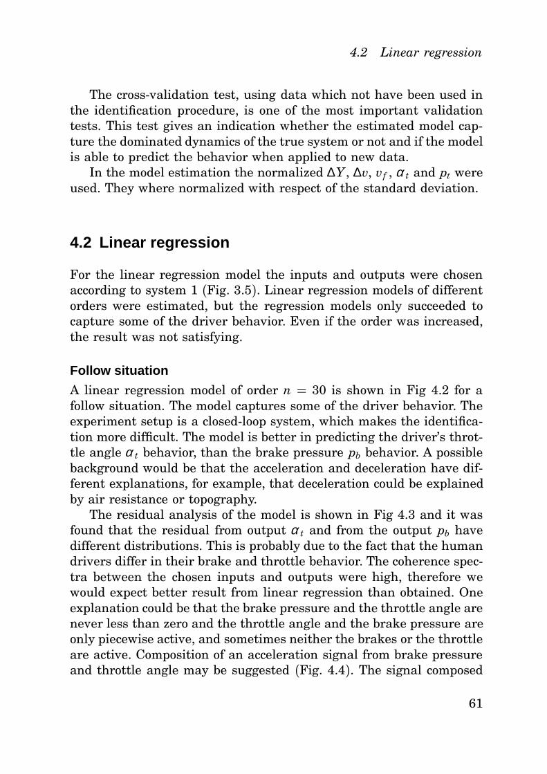
4.2 Linear regression
The cross-validation test, using data which not have been used inthe identification procedure, is one of the most important validationtests. This test gives an indication whether the estimated model cap-ture the dominated dynamics of the true system or not and if the modelis able to predict the behavior when applied to new data.
In the model estimation the normalized ∆Y , ∆v, vf , α t and pt wereused. They where normalized with respect of the standard deviation.
4.2 Linear regression
For the linear regression model the inputs and outputs were chosenaccording to system 1 (Fig. 3.5). Linear regression models of differentorders were estimated, but the regression models only succeeded tocapture some of the driver behavior. Even if the order was increased,the result was not satisfying.
Follow situation
A linear regression model of order n = 30 is shown in Fig 4.2 for afollow situation. The model captures some of the driver behavior. Theexperiment setup is a closed-loop system, which makes the identifica-tion more difficult. The model is better in predicting the driver’s throt-tle angle α t behavior, than the brake pressure pb behavior. A possiblebackground would be that the acceleration and deceleration have dif-ferent explanations, for example, that deceleration could be explainedby air resistance or topography.
The residual analysis of the model is shown in Fig 4.3 and it wasfound that the residual from output α t and from the output pb havedifferent distributions. This is probably due to the fact that the humandrivers differ in their brake and throttle behavior. The coherence spec-tra between the chosen inputs and outputs were high, therefore wewould expect better result from linear regression than obtained. Oneexplanation could be that the brake pressure and the throttle angle arenever less than zero and the throttle angle and the brake pressure areonly piecewise active, and sometimes neither the brakes or the throttleare active. Composition of an acceleration signal from brake pressureand throttle angle may be suggested (Fig. 4.4). The signal composed
61
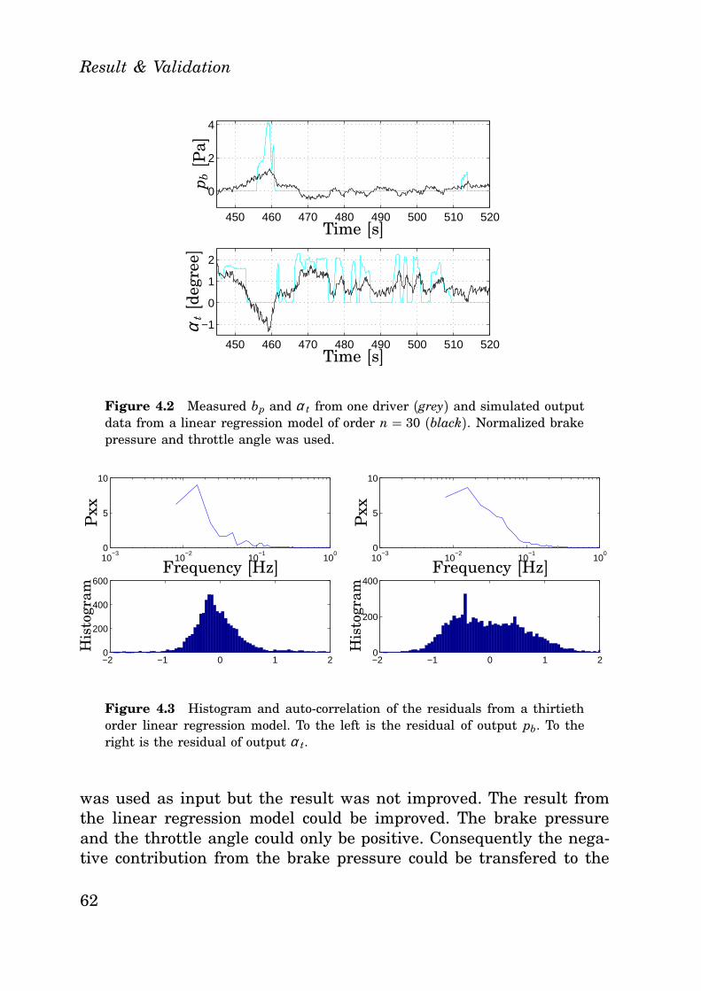
Result & Validation
450 460 470 480 490 500 510 520
0
2
4
450 460 470 480 490 500 510 520
−1
0
1
2
Time [s]
Time [s]p b[P
a]α
t[d
egre
e]
Figure 4.2 Measured bp and α t from one driver (grey) and simulated outputdata from a linear regression model of order n = 30 (black). Normalized brakepressure and throttle angle was used.
10−3
10−2
10−1
100
0
5
10
−2 −1 0 1 20
200
400
600Frequency [Hz]
Pxx
His
togr
am
10−3
10−2
10−1
100
0
5
10
−2 −1 0 1 20
200
400Frequency [Hz]
Pxx
His
togr
am
Figure 4.3 Histogram and auto-correlation of the residuals from a thirtiethorder linear regression model. To the left is the residual of output pb. To theright is the residual of output α t.
was used as input but the result was not improved. The result fromthe linear regression model could be improved. The brake pressureand the throttle angle could only be positive. Consequently the nega-tive contribution from the brake pressure could be transfered to the
62
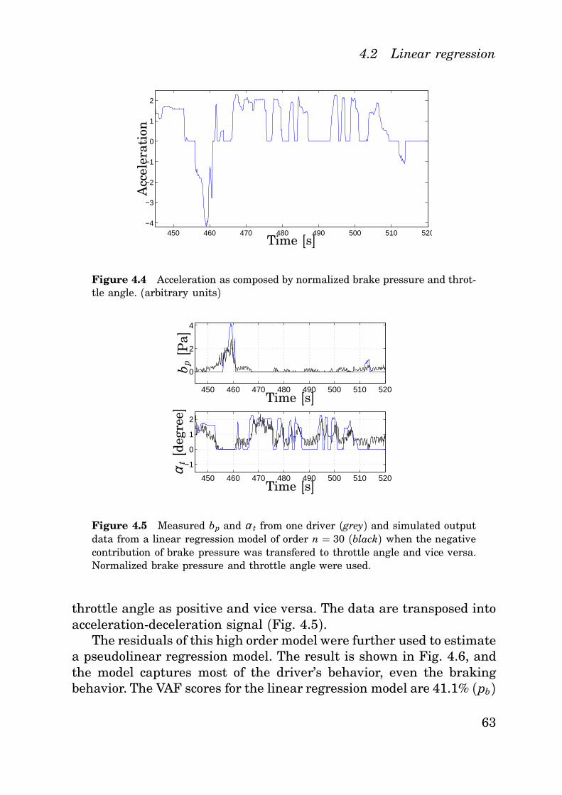
4.2 Linear regression
450 460 470 480 490 500 510 520−4
−3
−2
−1
0
1
2
Time [s]
Acc
eler
atio
n
Figure 4.4 Acceleration as composed by normalized brake pressure and throt-tle angle. (arbitrary units)
450 460 470 480 490 500 510 520
0
2
4
450 460 470 480 490 500 510 520
−1
0
1
2
Time [s]
Time [s]
αt[d
egre
e]b p[P
a]
Figure 4.5 Measured bp and α t from one driver (grey) and simulated outputdata from a linear regression model of order n = 30 (black) when the negativecontribution of brake pressure was transfered to throttle angle and vice versa.Normalized brake pressure and throttle angle were used.
throttle angle as positive and vice versa. The data are transposed intoacceleration-deceleration signal (Fig. 4.5).
The residuals of this high order model were further used to estimatea pseudolinear regression model. The result is shown in Fig. 4.6, andthe model captures most of the driver’s behavior, even the brakingbehavior. The VAF scores for the linear regression model are 41.1% (pb)
63
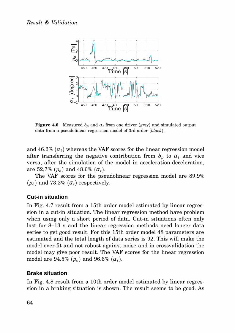
Result & Validation
450 460 470 480 490 500 510 520
0
2
4
450 460 470 480 490 500 510 520−1
0
1
2
3
Time [s]
Time [s]p b[P
a]α
t[d
egre
e]
Figure 4.6 Measured bp and α t from one driver (grey) and simulated outputdata from a pseudolinear regression model of 3rd order (black).
and 46.2% (α t) whereas the VAF scores for the linear regression modelafter transferring the negative contribution from bp to α t and viceversa, after the simulation of the model in acceleration-deceleration,are 52,7% (pb) and 48.6% (α t).
The VAF scores for the pseudolinear regression model are 89.9%(pb) and 73.2% (α t) respectively.
Cut-in situation
In Fig. 4.7 result from a 15th order model estimated by linear regres-sion in a cut-in situation. The linear regression method have problemwhen using only a short period of data. Cut-in situations often onlylast for 8–13 s and the linear regression methods need longer dataseries to get good result. For this 15th order model 48 parameters areestimated and the total length of data series is 92. This will make themodel over-fit and not robust against noise and in crossvalidation themodel may give poor result. The VAF scores for the linear regressionmodel are 94.5% (pb) and 96.6% (α t).
Brake situation
In Fig. 4.8 result from a 10th order model estimated by linear regres-sion in a braking situation is shown. The result seems to be good. As
64

4.2 Linear regression
0 2 4 6 8 10−2
0
2
4
Bra
ke p
ress
ure
(Pa)
0 2 4 6 8 10−2
0
2
4T
hrot
tle a
ngle
(de
gree
)
Time [s]
Time [s]
Figure 4.7 Cut-in: measured bp and α t from one driver (grey) and simulatedoutput data from a linear regression model of 15th order (black).
0 1 2 3 4 5 6 7−2
0
2
4
Bra
ke p
ress
ure
(Pa)
0 1 2 3 4 5 6 7−2
0
2
4
Time [s]
Thr
ottle
ang
le (
degr
ee)
Figure 4.8 Brake: normalized bp and α t from one driver (solid) and simulatedoutput data from a linear regression model of 10th order (dashed).
for the cut-in situations, the model tends to be over-fitted and not ro-bust against noise. The VAF scores for the linear regression model are97.4% (pb) and 99.9% (α t).
Approaching situation
In Fig. 4.9 result from a 15th order model estimated by linear regres-sion in a approaching situation is shown. The approaching situation
65
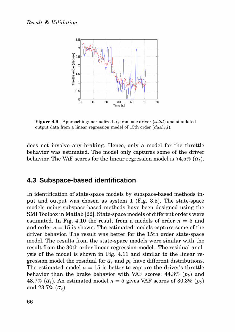
Result & Validation
0 10 20 30 40 50 600
0.5
1
1.5
2
2.5
3
3.5
Time [s]
Thr
ottle
ang
le (
degr
ee)
Figure 4.9 Approaching: normalized α t from one driver (solid) and simulatedoutput data from a linear regression model of 15th order (dashed).
does not involve any braking. Hence, only a model for the throttlebehavior was estimated. The model only captures some of the driverbehavior. The VAF scores for the linear regression model is 74,5% (α t).
4.3 Subspace-based identification
In identification of state-space models by subspace-based methods in-put and output was chosen as system 1 (Fig. 3.5). The state-spacemodels using subspace-based methods have been designed using theSMI Toolbox in Matlab [22]. State-space models of different orders wereestimated. In Fig. 4.10 the result from a models of order n = 5 andand order n = 15 is shown. The estimated models capture some of thedriver behavior. The result was better for the 15th order state-spacemodel. The results from the state-space models were similar with theresult from the 30th order linear regression model. The residual anal-ysis of the model is shown in Fig. 4.11 and similar to the linear re-gression model the residual for α t and pb have different distributions.The estimated model n = 15 is better to capture the driver’s throttlebehavior than the brake behavior with VAF scores: 44.3% (pb) and48.7% (α t). An estimated model n = 5 gives VAF scores of 30.3% (pb)and 23.7% (α t).
66
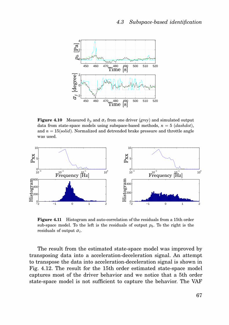
4.3 Subspace-based identification
450 460 470 480 490 500 510 520
0
2
4
450 460 470 480 490 500 510 520
−2
0
2
Time [s]
Time [s]p b[P
a]α
t[d
egre
e]
Figure 4.10 Measured bp and α t from one driver (grey) and simulated outputdata from state-space models using subspace-based methods, n = 5 (dashdot),and n = 15(solid). Normalized and detrended brake pressure and throttle anglewas used.
10−3
10−2
10−1
100
0
5
10
−2 −1 0 1 20
200
400
600Frequency [Hz]
Pxx
His
togr
am
10−3
10−2
10−1
100
0
5
10
−2 −1 0 1 20
200
400
Frequency [Hz]
Pxx
His
togr
am
Figure 4.11 Histogram and auto-correlation of the residuals from a 15th ordersub-space model. To the left is the residuals of output pb. To the right is theresiduals of output α t.
The result from the estimated state-space model was improved bytransposing data into a acceleration-deceleration signal. An attemptto transpose the data into acceleration-deceleration signal is shown inFig. 4.12. The result for the 15th order estimated state-space modelcaptures most of the driver behavior and we notice that a 5th orderstate-space model is not sufficient to capture the behavior. The VAF
67
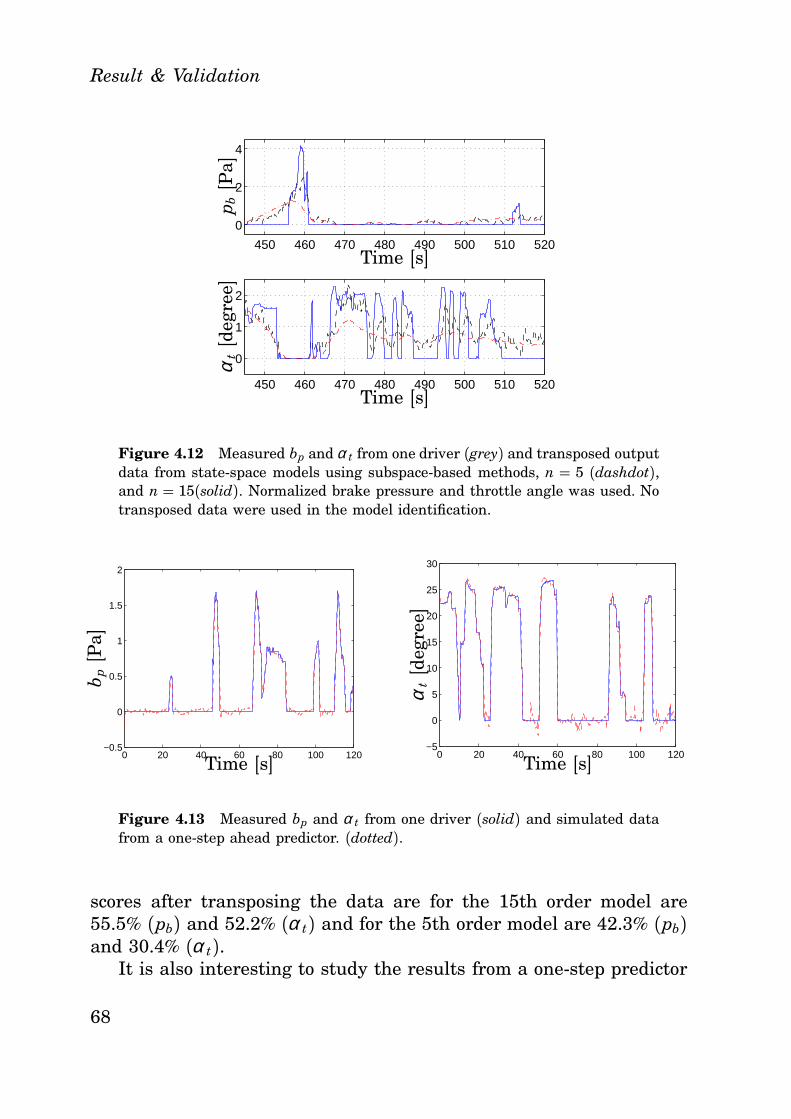
Result & Validation
450 460 470 480 490 500 510 520
0
2
4
450 460 470 480 490 500 510 520
0
1
2
Time [s]
Time [s]p b[P
a]α
t[d
egre
e]
Figure 4.12 Measured bp and α t from one driver (grey) and transposed outputdata from state-space models using subspace-based methods, n = 5 (dashdot),and n = 15(solid). Normalized brake pressure and throttle angle was used. Notransposed data were used in the model identification.
0 20 40 60 80 100 120−0.5
0
0.5
1
1.5
2
Time [s]
b p[P
a]
0 20 40 60 80 100 120−5
0
5
10
15
20
25
30
Time [s]
αt[d
egre
e]
Figure 4.13 Measured bp and α t from one driver (solid) and simulated datafrom a one-step ahead predictor. (dotted).
scores after transposing the data are for the 15th order model are55.5% (pb) and 52.2% (α t) and for the 5th order model are 42.3% (pb)and 30.4% (α t).
It is also interesting to study the results from a one-step predictor
68
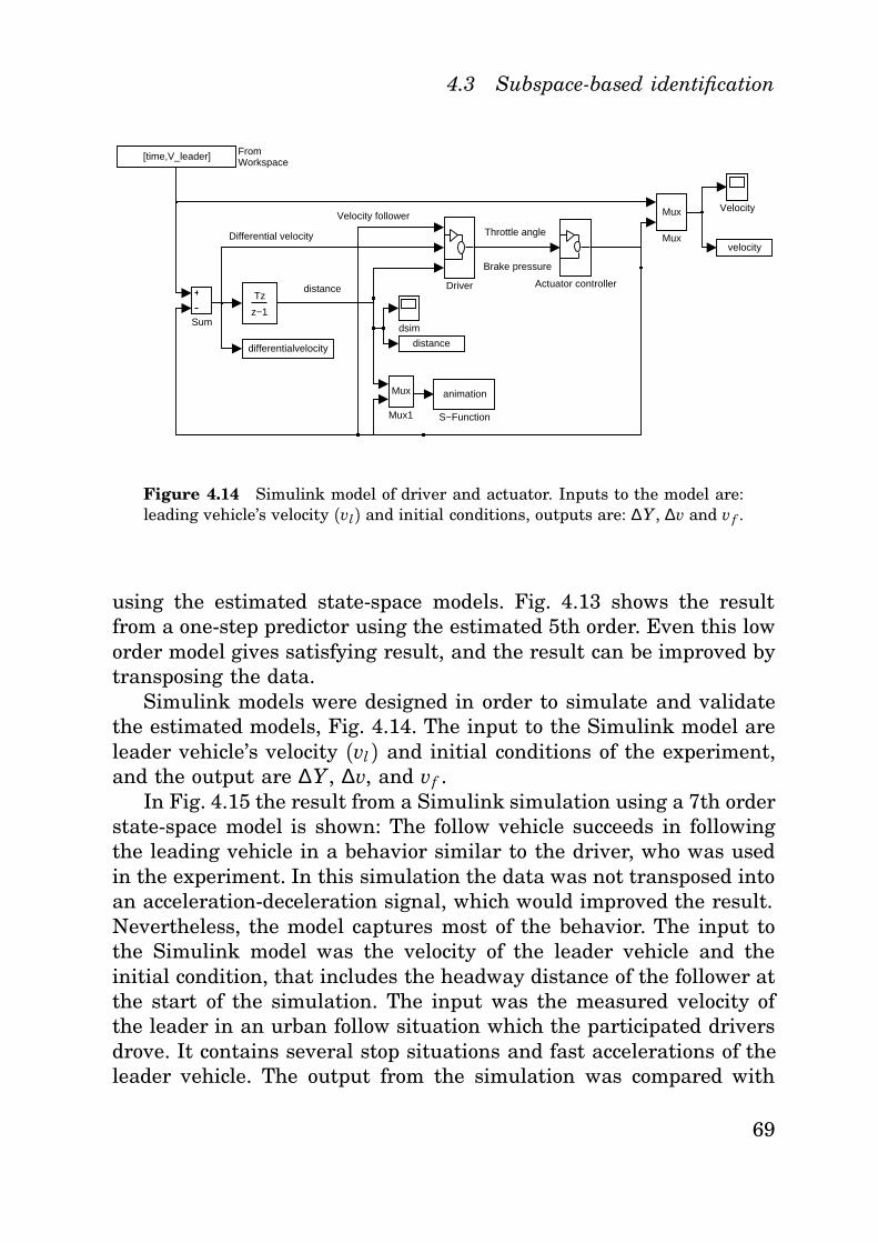
4.3 Subspace-based identification
Throttle angle
Brake pressure
distance
Differential velocity
Velocity follower
dsim
Velocity
Sum
animation
S−Function
Mux
Mux1
Mux
Mux
[time,V_leader] FromWorkspace
Driver Actuator controller
differentialvelocity
velocity
distance
Tz
z−1
Figure 4.14 Simulink model of driver and actuator. Inputs to the model are:leading vehicle’s velocity (vl) and initial conditions, outputs are: ∆Y, ∆v and vf .
using the estimated state-space models. Fig. 4.13 shows the resultfrom a one-step predictor using the estimated 5th order. Even this loworder model gives satisfying result, and the result can be improved bytransposing the data.
Simulink models were designed in order to simulate and validatethe estimated models, Fig. 4.14. The input to the Simulink model areleader vehicle’s velocity (vl) and initial conditions of the experiment,and the output are ∆Y , ∆v, and vf .
In Fig. 4.15 the result from a Simulink simulation using a 7th orderstate-space model is shown: The follow vehicle succeeds in followingthe leading vehicle in a behavior similar to the driver, who was usedin the experiment. In this simulation the data was not transposed intoan acceleration-deceleration signal, which would improved the result.Nevertheless, the model captures most of the behavior. The input tothe Simulink model was the velocity of the leader vehicle and theinitial condition, that includes the headway distance of the follower atthe start of the simulation. The input was the measured velocity ofthe leader in an urban follow situation which the participated driversdrove. It contains several stop situations and fast accelerations of theleader vehicle. The output from the simulation was compared with
69
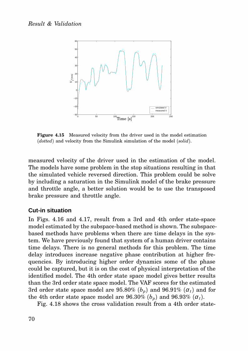
Result & Validation
0 50 100 150 200 250−30
−20
−10
0
10
20
30
40
50
60
[m/s
]
simulated Vmeasured V
Time [s]
Vf
Figure 4.15 Measured velocity from the driver used in the model estimation(dotted) and velocity from the Simulink simulation of the model (solid).
measured velocity of the driver used in the estimation of the model.The models have some problem in the stop situations resulting in thatthe simulated vehicle reversed direction. This problem could be solveby including a saturation in the Simulink model of the brake pressureand throttle angle, a better solution would be to use the transposedbrake pressure and throttle angle.
Cut-in situation
In Figs. 4.16 and 4.17, result from a 3rd and 4th order state-spacemodel estimated by the subspace-based method is shown. The subspace-based methods have problems when there are time delays in the sys-tem. We have previously found that system of a human driver containstime delays. There is no general methods for this problem. The timedelay introduces increase negative phase contribution at higher fre-quencies. By introducing higher order dynamics some of the phasecould be captured, but it is on the cost of physical interpretation of theidentified model. The 4th order state space model gives better resultsthan the 3rd order state space model. The VAF scores for the estimated3rd order state space model are 95.80% (bp) and 96.91% (α t) and forthe 4th order state space model are 96.30% (bp) and 96.93% (α t).
Fig. 4.18 shows the cross validation result from a 4th order state-
70
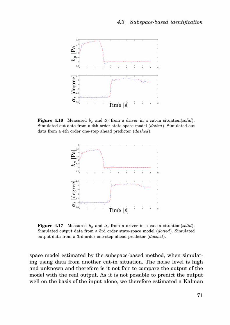
4.3 Subspace-based identification
0 1 2 3 4 5 6 7 8 9 10−0.5
0
0.5
1
1.5
2
2.5
0 1 2 3 4 5 6 7 8 9 10−0.5
0
0.5
1
1.5
2
2.5b p[P
a]
Time [s]αt[d
egre
e]
Figure 4.16 Measured bp and α t from a driver in a cut-in situation(solid).Simulated out data from a 4th order state-space model (dotted). Simulated outdata from a 4th order one-step ahead predictor (dashed).
0 1 2 3 4 5 6 7 8 9 10−0.5
0
0.5
1
1.5
2
2.5
3
0 1 2 3 4 5 6 7 8 9 10−0.5
0
0.5
1
1.5
2
2.5
b p[P
a]
Time [s]αt[d
egre
e]
Figure 4.17 Measured bp and α t from a driver in a cut-in situation(solid).Simulated output data from a 3rd order state-space model (dotted). Simulatedoutput data from a 3rd order one-step ahead predictor (dashed).
space model estimated by the subspace-based method, when simulat-ing using data from another cut-in situation. The noise level is highand unknown and therefore is it not fair to compare the output of themodel with the real output. As it is not possible to predict the outputwell on the basis of the input alone, we therefore estimated a Kalman
71
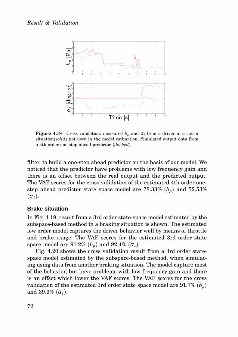
Result & Validation
0 1 2 3 4 5 6 7 8 9 10−1
0
1
2
3
4
0 1 2 3 4 5 6 7 8 9 10−3
−2
−1
0
1
2
3
b p[P
a]
Time [s]
αt[d
egre
e]
Figure 4.18 Cross validation: measured bp and α t from a driver in a cut-insituation(solid) not used in the model estimation. Simulated output data froma 4th order one-step ahead predictor (dashed).
filter, to build a one-step ahead predictor on the basis of our model. Wenoticed that the predictor have problems with low frequency gain andthere is an offset between the real output and the predicted output.The VAF scores for the cross validation of the estimated 4th order one-step ahead predictor state space model are 78.33% (bp) and 52.53%(α t).
Brake situation
In Fig. 4.19, result from a 3rd order state-space model estimated by thesubspace-based method in a braking situation is shown. The estimatedlow order model captures the driver behavior well by means of throttleand brake usage. The VAF scores for the estimated 3rd order statespace model are 91.2% (bp) and 92.4% (α t).
Fig. 4.20 shows the cross validation result from a 3rd order state-space model estimated by the subspace-based method, when simulat-ing using data from another braking situation. The model capture mostof the behavior, but have problems with low frequency gain and thereis an offset which lower the VAF scores. The VAF scores for the crossvalidation of the estimated 3rd order state space model are 91.7% (bp)and 39.3% (α t).
72
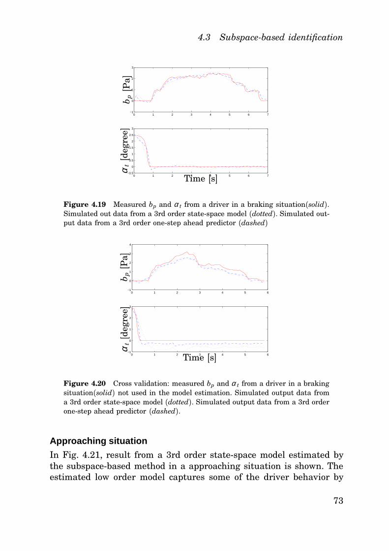
4.3 Subspace-based identification
0 1 2 3 4 5 6 7−1
0
1
2
3
0 1 2 3 4 5 6 7−0.5
0
0.5
1
1.5
2
2.5
3b p[P
a]
Time [s]αt[d
egre
e]
Figure 4.19 Measured bp and α t from a driver in a braking situation(solid).Simulated out data from a 3rd order state-space model (dotted). Simulated out-put data from a 3rd order one-step ahead predictor (dashed)
0 1 2 3 4 5 6−1
0
1
2
3
4
0 1 2 3 4 5 6−1
0
1
2
3
b p[P
a]
Time [s]
αt[d
egre
e]
Figure 4.20 Cross validation: measured bp and α t from a driver in a brakingsituation(solid) not used in the model estimation. Simulated output data froma 3rd order state-space model (dotted). Simulated output data from a 3rd orderone-step ahead predictor (dashed).
Approaching situation
In Fig. 4.21, result from a 3rd order state-space model estimated bythe subspace-based method in a approaching situation is shown. Theestimated low order model captures some of the driver behavior by
73
Result & Validation
0 5 10 15 20 25 30 35 40 45 50 55
0
0.5
1
1.5
2
2.5
3
3.5
Time [s]
αt[d
egre
e]
Figure 4.21 Approaching: measured α t from one driver (solid) and simulatedoutput data from a 3:rd order state-space model(dashed).
means of throttle usage. The VAF scores for the estimated 3rd orderstate space model is 80.9% (α t).
String stability
For application in automated highway it is necessary that a stream ofcars are string stable, i. e., if several vehicles are put in a row theyshould not give rise to oscillation causing car crashes [46]. Fig. 4.22shows Simulink simulation result from a follow situation where 6 ve-hicles have been put in a row. Each vehicle is controlled by a 5th ordermodel identified using the subspace-based method. No crash occursin the simulation, but the oscillations grow in magnitude. Previoussimulation results show that a 15th order state-space model capturesthe driving behavior significantly better than a 5th order state-spacemodel and that the result can be improved using transposed signals.
4.4 Behavioral model
For the behavioral models the inputs and outputs were chosen accord-ing to system 2 (Fig. 3.5). Behavioral model of different order whereestimated. The estimated model including both dynamic of the input
74
4.4 Behavioral model
0 100 200 300 400 500 600 700 800 900 100010
15
20
25
30
35
Time [s]
∆Y[m]
0 100 200 300 400 500 600 700 800 900 1000−10
0
10
20
30
40
50
60
Time [s]
v f[k
m/h]
Figure 4.22 Result from a Simulink simulation with 6 vehicles in row. ∆Ybetween the vehicles (left) and vf of the vehicles (right).
and the outputs, since the model does not explicitly separate the sig-nals into inputs and outputs, which is an advantage in the identifica-tion process since there are interactions between the driver and thevehicle.
Follow situation
In Fig. 4.23 a model with the total order of 30 is shown. The model fitsthe driver behavior well capturing both the braking behavior and thethrottle behavior.
The residual analysis of the estimated 30th order model basedon the behavior method is shown in Fig. 4.24. Both brake pressureand throttle angle have empirical distributions comparable with nor-mal distributions. The VAF scores for the behavioral model are 81.9%(pb) and 92.2% (α t). In order to use the estimated model in an ACC-approach it is necessary to obtain from the estimated model, whichcontain dynamics both of the inputs and the outputs as well as theexperimental condition, a input-output relation according to system 1(Fig. 3.5). The transfer function for the input-output can be obtainedby matrix fraction decomposition, but this is not a easily solved prob-lem, since the estimated model can be divided into submodels and wewant to find the subsystem which best matches the inputs and theoutputs. This problem is not yet solved.
75
Result & Validation
440 460 480 500 520
0
5
10
15
440 460 480 500 520
0
5
10
15
Time [s]
Time [s]
p b[P
a]α
t[d
egre
e]
Figure 4.23 Follow: measured bp and α t from one driver (grey) and simulatedoutput data from a behavioral model order n = 30 (black).
10−3
10−2
10−1
100
0
5
10
−2 −1 0 1 20
50
100
440 460 480 500 520
−5
0
5
Frequency [Hz]
Time [s]
Pxx
His
togr
amR
esid
uals
10−3
10−2
10−1
100
0
5
10
15
−2 −1 0 1 20
20
40
440 460 480 500 520
−5
0
5
Frequency [Hz]
Time [s]
Pxx
His
togr
amR
esid
uals
Figure 4.24 Residuals of output pb from a behavior model n = 30 (left). Resid-uals of output α t from a behavior model n = 30 (right). Notice that the residualof the output pb becomes large when the time is around 460s.
76
4.4 Behavioral model
−3 −2.5 −2 −1.5 −1 −0.5 0 0.5 19
9.5
10
10.5
11
11.5
12
12.5
13
13.5
14
∆Y[m]
∆v [km/s] −2.5 −2 −1.5 −1 −0.5 0 0.5 114.5
15
15.5
16
16.5
17
17.5
18
18.5
19
∆Y[m]
∆v [km/s]
Figure 4.25 Cut-in: measured ∆Y and ∆v (solid) and simulated ∆Y and ∆vfrom a behavioral model of order n = 10 (dotted). Driver 1 (left) and driver 2(right)
0 1 2 3 4 5 6 7−10
0
10
20
0 1 2 3 4 5 6 7−10
0
10
20
Time [s]
p b[P
a]α
t[d
egre
e]
Cut-in situation 1
0 2 4 6 8−10
0
10
20
0 2 4 6 8−10
0
10
20
Time [s]
p b[P
a]α
t[d
egre
e]
Cut-in situation 2
Figure 4.26 Cut-in: measured bp and α t from one driver (solid) and simulatedoutput data from a behavioral model n = 10 (dotted).
Cut-in situation
Figs 4.25 and 4.26 show result from a estimated behavioral models oforder n = 10 estimated from data from a cut-in situation. The model fitthe measured data well, but one problem capture the driver behavior incut-in situations is that they last only a short period of time resultingin a short data sequence. By only studying the data and the result from
77
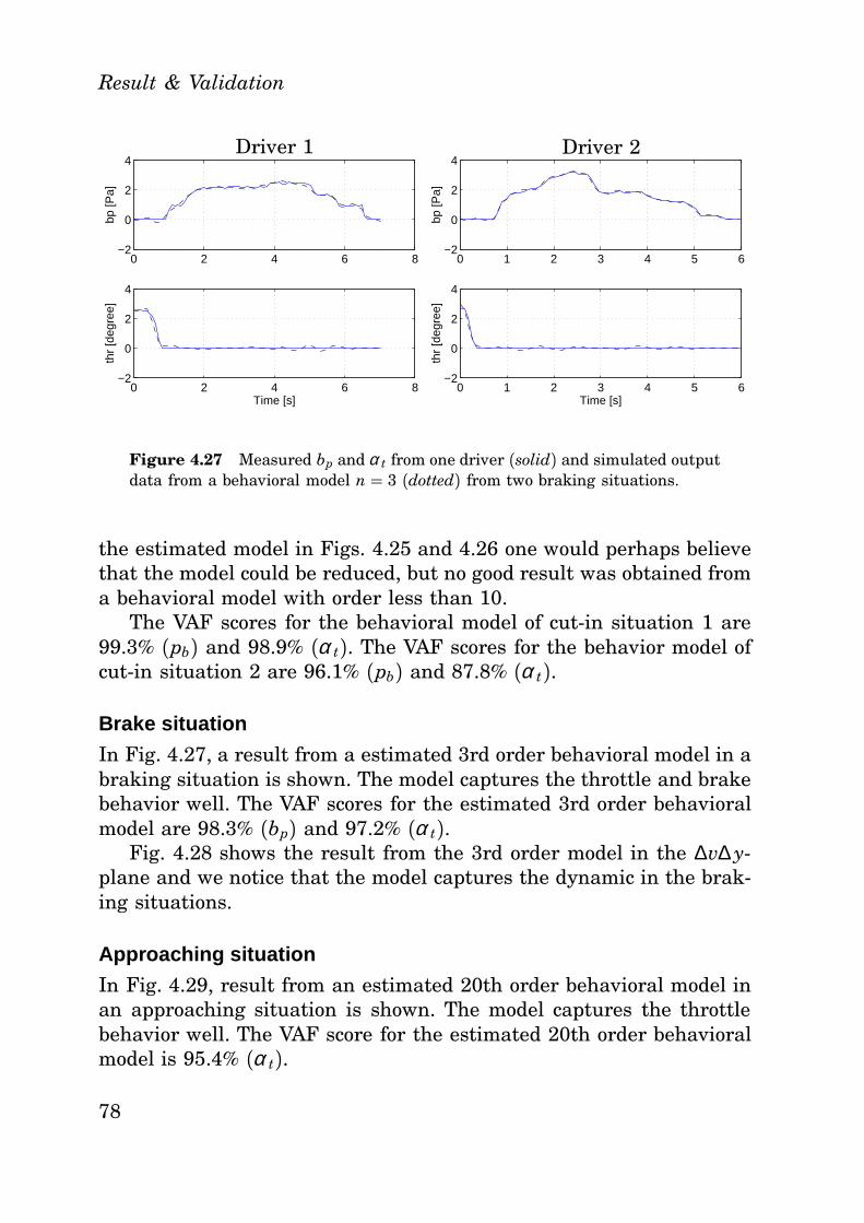
Result & Validation
0 2 4 6 8−2
0
2
4
bp [P
a]
0 2 4 6 8−2
0
2
4
Time [s]
thr
[deg
ree]
Driver 1
0 1 2 3 4 5 6−2
0
2
4
bp [P
a]
0 1 2 3 4 5 6−2
0
2
4
Time [s]
thr
[deg
ree]
Driver 2
Figure 4.27 Measured bp and α t from one driver (solid) and simulated outputdata from a behavioral model n = 3 (dotted) from two braking situations.
the estimated model in Figs. 4.25 and 4.26 one would perhaps believethat the model could be reduced, but no good result was obtained froma behavioral model with order less than 10.
The VAF scores for the behavioral model of cut-in situation 1 are99.3% (pb) and 98.9% (α t). The VAF scores for the behavior model ofcut-in situation 2 are 96.1% (pb) and 87.8% (α t).
Brake situation
In Fig. 4.27, a result from a estimated 3rd order behavioral model in abraking situation is shown. The model captures the throttle and brakebehavior well. The VAF scores for the estimated 3rd order behavioralmodel are 98.3% (bp) and 97.2% (α t).
Fig. 4.28 shows the result from the 3rd order model in the ∆v∆ y-plane and we notice that the model captures the dynamic in the brak-ing situations.
Approaching situation
In Fig. 4.29, result from an estimated 20th order behavioral model inan approaching situation is shown. The model captures the throttlebehavior well. The VAF score for the estimated 20th order behavioralmodel is 95.4% (α t).
78
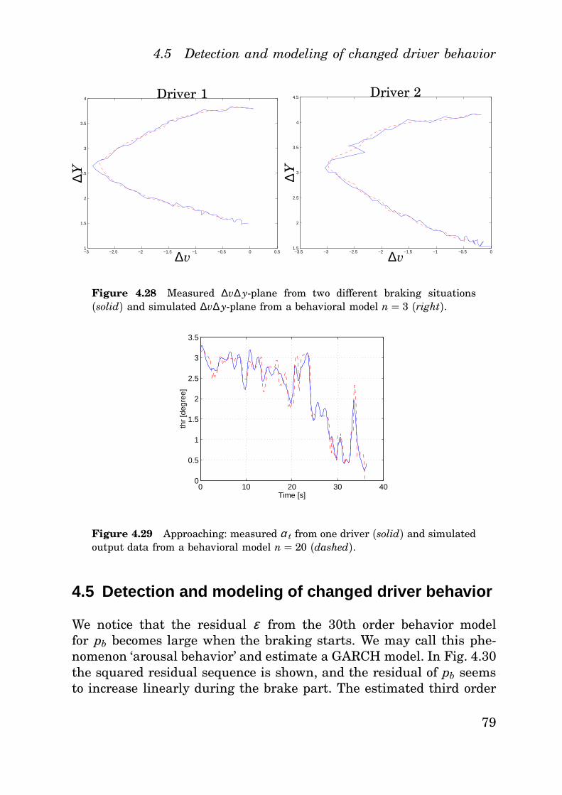
4.5 Detection and modeling of changed driver behavior
−3 −2.5 −2 −1.5 −1 −0.5 0 0.51
1.5
2
2.5
3
3.5
4
∆v
∆Y
Driver 1
−3.5 −3 −2.5 −2 −1.5 −1 −0.5 01.5
2
2.5
3
3.5
4
4.5
∆v
∆Y
Driver 2
Figure 4.28 Measured ∆v∆ y-plane from two different braking situations(solid) and simulated ∆v∆ y-plane from a behavioral model n = 3 (right).
0 10 20 30 400
0.5
1
1.5
2
2.5
3
3.5
Time [s]
thr
[deg
ree]
Figure 4.29 Approaching: measured α t from one driver (solid) and simulatedoutput data from a behavioral model n = 20 (dashed).
4.5 Detection and modeling of changed driver behavior
We notice that the residual ε from the 30th order behavior modelfor pb becomes large when the braking starts. We may call this phe-nomenon ‘arousal behavior’ and estimate a GARCH model. In Fig. 4.30the squared residual sequence is shown, and the residual of pb seemsto increase linearly during the brake part. The estimated third order
79
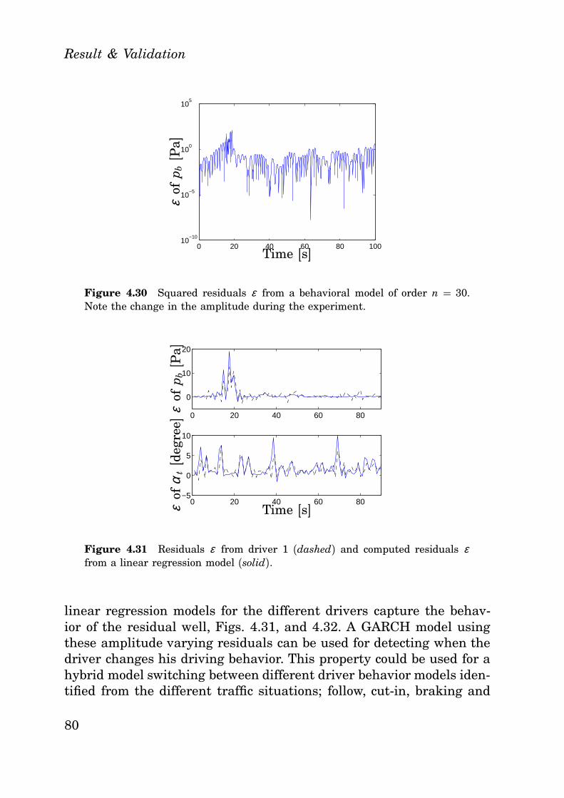
Result & Validation
0 20 40 60 80 10010
−10
10−5
100
105
Time [s]
εof
p b[P
a]
Figure 4.30 Squared residuals ε from a behavioral model of order n = 30.Note the change in the amplitude during the experiment.
0 20 40 60 80
0
10
20
0 20 40 60 80−5
0
5
10
Time [s]
εof
p b[P
a]ε
ofα
t[d
egre
e]
Figure 4.31 Residuals ε from driver 1 (dashed) and computed residuals εfrom a linear regression model (solid).
linear regression models for the different drivers capture the behav-ior of the residual well, Figs. 4.31, and 4.32. A GARCH model usingthese amplitude varying residuals can be used for detecting when thedriver changes his driving behavior. This property could be used for ahybrid model switching between different driver behavior models iden-tified from the different traffic situations; follow, cut-in, braking and
80
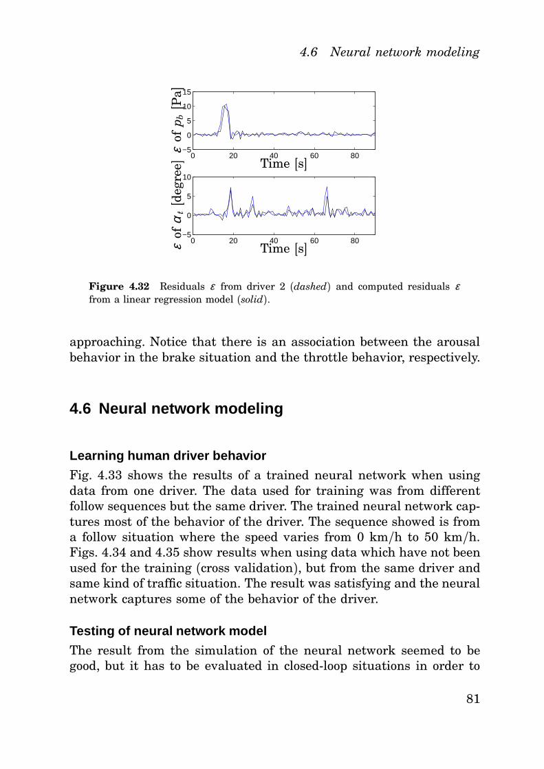
4.6 Neural network modeling
0 20 40 60 80−5
0
5
10
15
0 20 40 60 80−5
0
5
10
Time [s]
Time [s]ε
ofp b[P
a]ε
ofα
t[d
egre
e]
Figure 4.32 Residuals ε from driver 2 (dashed) and computed residuals εfrom a linear regression model (solid).
approaching. Notice that there is an association between the arousalbehavior in the brake situation and the throttle behavior, respectively.
4.6 Neural network modeling
Learning human driver behavior
Fig. 4.33 shows the results of a trained neural network when usingdata from one driver. The data used for training was from differentfollow sequences but the same driver. The trained neural network cap-tures most of the behavior of the driver. The sequence showed is froma follow situation where the speed varies from 0 km/h to 50 km/h.Figs. 4.34 and 4.35 show results when using data which have not beenused for the training (cross validation), but from the same driver andsame kind of traffic situation. The result was satisfying and the neuralnetwork captures some of the behavior of the driver.
Testing of neural network model
The result from the simulation of the neural network seemed to begood, but it has to be evaluated in closed-loop situations in order to
81
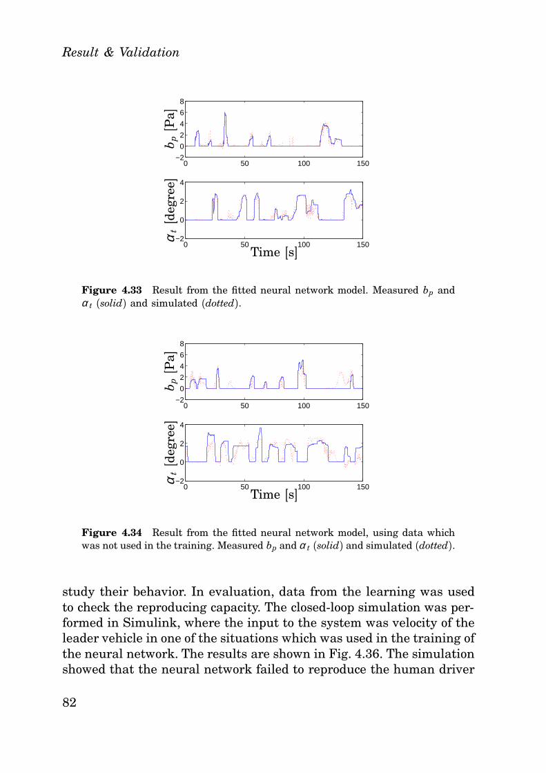
Result & Validation
0 50 100 150−2
0
2
4
6
8
0 50 100 150−2
0
2
4
Time [s]
b p[P
a]α
t[d
egre
e]
Figure 4.33 Result from the fitted neural network model. Measured bp andα t (solid) and simulated (dotted).
0 50 100 150−2
0
2
4
6
8
0 50 100 150−2
0
2
4
Time [s]
b p[P
a]α
t[d
egre
e]
Figure 4.34 Result from the fitted neural network model, using data whichwas not used in the training. Measured bp and α t (solid) and simulated (dotted).
study their behavior. In evaluation, data from the learning was usedto check the reproducing capacity. The closed-loop simulation was per-formed in Simulink, where the input to the system was velocity of theleader vehicle in one of the situations which was used in the training ofthe neural network. The results are shown in Fig. 4.36. The simulationshowed that the neural network failed to reproduce the human driver
82
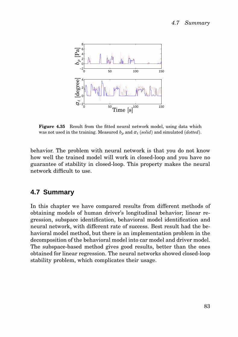
4.7 Summary
0 50 100 150−2
0
2
4
6
8
0 50 100 150−2
0
2
4
Time [s]
b p[P
a]α
t[d
egre
e]
Figure 4.35 Result from the fitted neural network model, using data whichwas not used in the training. Measured bp and α t (solid) and simulated (dotted).
behavior. The problem with neural network is that you do not knowhow well the trained model will work in closed-loop and you have noguarantee of stability in closed-loop. This property makes the neuralnetwork difficult to use.
4.7 Summary
In this chapter we have compared results from different methods ofobtaining models of human driver’s longitudinal behavior; linear re-gression, subspace identification, behavioral model identification andneural network, with different rate of success. Best result had the be-havioral model method, but there is an implementation problem in thedecomposition of the behavioral model into car model and driver model.The subspace-based method gives good results, better than the onesobtained for linear regression. The neural networks showed closed-loopstability problem, which complicates their usage.
83
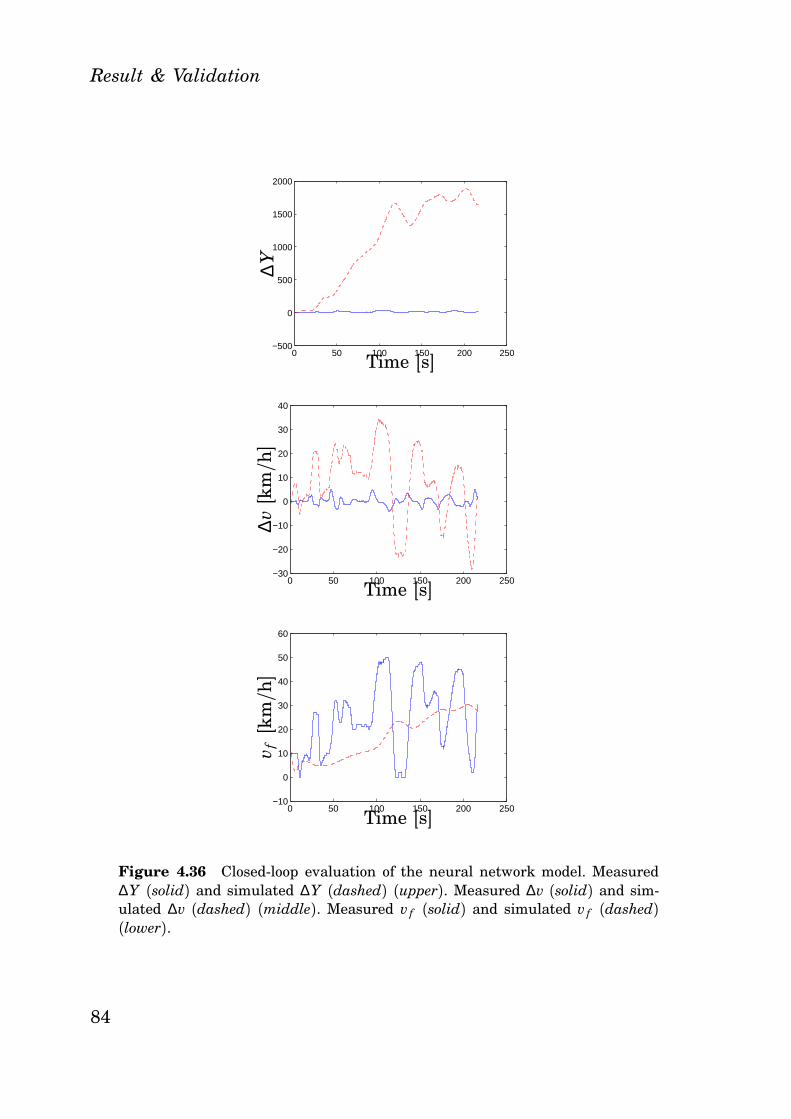
Result & Validation
0 50 100 150 200 250−500
0
500
1000
1500
2000
Time [s]
∆Y
0 50 100 150 200 250−30
−20
−10
0
10
20
30
40
Time [s]
∆v[k
m/h]
0 50 100 150 200 250−10
0
10
20
30
40
50
60
Time [s]
v f[k
m/h]
Figure 4.36 Closed-loop evaluation of the neural network model. Measured∆Y (solid) and simulated ∆Y (dashed) (upper). Measured ∆v (solid) and sim-ulated ∆v (dashed) (middle). Measured vf (solid) and simulated vf (dashed)(lower).
84

5
Discussion & Conclusions
5.1 Discussion
Human drivers use several sensors in the driving tasks: eyesight, hear-ing, balance organ (vestibular organ of the inner ear; vestibular nu-clei), and proprioception. The central nervous system fuses the infor-mation from the sensors [31]. The vestibular system nuclei and pro-prioception detect changes in orientation, position and acceleration.These physological human sensors can be translated into: camera, mi-crophone, gyro, and accelerometer. As the information rate must bemanageable and since the total information rate from the sensors ishuge, it is not reasonable to measure all such information.
Sensors have different significance. The eyesight (vision) is themost important sensor a human driver uses in the driving task. Thus,for practical reasons only a laser and a radar were used in the exper-iments.
It is known that human sensors have bandpass properties [9], whichalso was found in the data analysis (Figs. 3.12, 3.13). The lower limitwas found around 0.1 Hz and the upper limit around 1.2 Hz. Thelower limit may be explained by visual suppression, which occur inthis region [39]. It has also been found that galvanic stimulation ofthe horizontal vestibulo-ocular reflex is not affected below 0.1 Hz [32].In other words, there exist other physiological evidence which explainthat a human driver exhibits bandpass properties. The upper limit
85
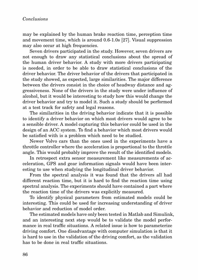
Conclusions
may be explained by the human brake reaction time, perception timeand movement time, which is around 0.6-1.0s [27]. Visual suppressionmay also occur at high frequencies.
Seven drivers participated in the study. However, seven drivers arenot enough to draw any statistical conclusions about the spread ofthe human driver behavior. A study with more drivers participatingis needed, in order to be able to draw statistical conclusions of thedriver behavior. The driver behavior of the drivers that participated inthe study showed, as expected, large similarities. The major differencebetween the drivers consist in the choice of headway distance and ag-gressiveness. None of the drivers in the study were under influence ofalcohol, but it would be interesting to study how this would change thedriver behavior and try to model it. Such a study should be performedat a test track for safety and legal reasons.
The similarities in the driving behavior indicate that it is possibleto identify a driver behavior on which most drivers would agree to bea sensible driver. A model capturing this behavior could be used in thedesign of an ACC system. To find a behavior which most drivers wouldbe satisfied with is a problem which need to be studied.
Newer Volvo cars than the ones used in the experiments have athrottle controller where the acceleration is proportional to the throttleangle. This would probably improve the result of the identified models.
In retrospect extra sensor measurement like measurements of ac-celeration, GPS and gear information signals would have been inter-esting to use when studying the longitudinal driver behavior.
From the spectral analysis it was found that the drivers all haddifferent reaction time, but it is hard to find the reaction time usingspectral analysis. The experiments should have contained a part wherethe reaction time of the drivers was explicitly measured.
To identify physical parameters from estimated models could beinteresting. This could be used for increasing understanding of driverbehavior and reduction of model order.
The estimated models have only been tested in Matlab and Simulink,and an interesting next step would be to validate the model perfor-mance in real traffic situations. A related issue is how to parameterizedriving comfort. One disadvantage with computer simulation is that itis hard to use in the validation of the driving comfort, as the validationhas to be done in real traffic situations.
86
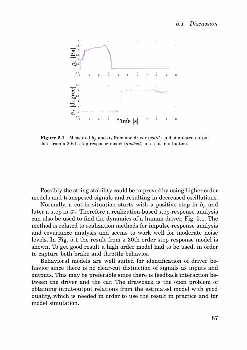
5.1 Discussion
0 1 2 3 4 5 6 7 8 9 10−0.5
0
0.5
1
1.5
2
2.5
3
0 1 2 3 4 5 6 7 8 9 10−0.5
0
0.5
1
1.5
2
2.5
Time [s]
p b[P
a]α
t[d
egre
e]
Figure 5.1 Measured bp and α t from one driver (solid) and simulated outputdata from a 30:th step response model (dashed) in a cut-in situation.
Possibly the string stability could be improved by using higher ordermodels and transposed signals and resulting in decreased oscillations.
Normally, a cut-in situation starts with a positive step in bp andlater a step in α t. Therefore a realization-based step-response analysiscan also be used to find the dynamics of a human driver, Fig. 5.1. Themethod is related to realization methods for impulse-response analysisand covariance analysis and seems to work well for moderate noiselevels. In Fig. 5.1 the result from a 30th order step response model isshown. To get good result a high order model had to be used, in orderto capture both brake and throttle behavior.
Behavioral models are well suited for identification of driver be-havior since there is no clear-cut distinction of signals as inputs andoutputs. This may be preferable since there is feedback interaction be-tween the driver and the car. The drawback is the open problem ofobtaining input-output relations from the estimated model with goodquality, which is needed in order to use the result in practice and formodel simulation.
87
Conclusions
5.2 Conclusions
One contribution of this thesis is to describe human driver longitudinalbehavior using dynamic models. Existing methods and models describ-ing human driver behavior have been reviewed: linear and non-lineardynamic car-following models, linear optimal control models, heuristicmodels, neural network and fuzzy logic models, mental models, andgeneral longitudinal models.
Another contribution is the application of existing identificationmethods to describe human driver’s longitudinal behavior. Linear re-gression, subspace model identification, behavioral models and neuralnetworks for finding dynamic models of human driver have been stud-ied, with varying results. The result of the proposed approach usingsystem identification was found satisfying. The models estimated havebeen simulated in closed-loop operation using Simulink with satisfy-ing result. The best result was found when using the behavioral modelmethod, but since the problem of obtaining an input-output relationfor the component models in open-loop operation, the practical use-fulness of the models are reduced. The estimated models using thesubspace-based methods did not give as good results as the behavioralmodels, but still better than the linear regression models. The model-ing of changes in driver behavior has been performed using GARCHmodels with satisfying results.
88
6
Bibliography
[1] P. S. Addison and D. J. Low. “A novel nonlinear car-followingmodel.” Chaos, 8:4, pp. 791–799, 1998.
[2] K. Ahmed. Modeling Drivers’ Acceleration and Lane ChangingBehavior. PhD thesis, Massachusetts Institute of Technology,Cambridge, 1999.
[3] B. D. O. Anderson and J. B. Moore. Optimal Control LinearQuadratic Methods. Prentice Hall, New Jersey, 1990.
[4] G. A. Bekey and G. O. Burnham. “Control theoretic models ofhuman drivers in car-following.” Human Factors, No 19, pp. 399–413, 1977.
[5] R. F. Benekohal and J. Treiterer. “Carsim: Car-following modelfor simulation of traffic in normal and stop-and-go conditions.”Transportation Research Record 1194, pp. pp. 99–111, 1998.
[6] T. Bleile. “A new microscopic model for car-following behavior inurban traffic.” In Proceedings 4th World Congress on IntelligentTransport Systems, Berlin, 1997.
[7] E. R. Boer and M. Hoedemaeker. “Modeling driver behaviorwith different degrees of automation: A hierarchical decisionframework of interacting mental models.” In Proceedings of theXVIIth European Conference on Human Decision Making andManual Control, Valenciennes, 1998.
[8] T. Bollerslev. “Generalized autoregressive conditional het-eroskedasticity.” J. of Econometrics, 31, pp. 307–327, 1986.
89
Chapter 6. Bibliography
[9] T. Brandt. Vertigo : Its Multisensory Syndromes. Springer, Berlin,2:nd edition, 1999.
[10] R. E. Chandler, R., Herman, and E. Montroll. “Traffic dynamics:studies in car following.” Operation Research, No 6, 1958.
[11] L. C. Edie, R. S. Foote, R. Herman, and R. Rorthery. “Analysisof single lane traffic flow.” Traffic Engineering 2, 33, pp. 21–27,1963.
[12] D. C. Gazis, R. Herman, and B. Potts. “Car-following theory ofsteady-state traffic flow.” Operation Research, No 9, 1959.
[13] D. C. Gazis, R. Herman, and R. W. Rothery. “Nonlinear follow-the-leader models of traffic flow.” Operation Research, No 9, 1961.
[14] S. Germann and R. Isermann. “Nonlinear distance and cruisecontrol for passenger cars.” In Proceedings of the AmericanControl Conference, vol. 1, pp. 3081–3085, 1995.
[15] A. Ghazi Zadeh, A. Fahim, and M. El-Gindy. “Neural networkand fuzzy logic applications to vehicle systems: literature survey.”Journal of Vehicle Design, 18:2, 1997.
[16] P. G. Gipps. “A behavioural car-following model for computersimulation.” Transport Research-B, 15, pp. 105–111, 1981.
[17] M. A. Goodrich and E. R. Boer. “Semiotics and mental models:Modeling automobile driver behavior.” In Proceeding of the 1998IEEE ISIC/CIRA/ISAS Joint Conference, pp. 771–776, Gaithers-burg, 1998.
[18] R. Gray and D. Regan. “Accuracy of estimating time to collisionusing binocular and monocular information.” Vision Research,pp. 499–512, 1998.
[19] N. C. Griswold, N. D. Kehtarnavaz, and K. M. Miller. “A trans-portable neural network controller for autonomous vehicle follow-ing.” In Intelligent Vehicles ’94 Symposium, pp. 195–200. 1994.
[20] M. T. Hagan and M. Menhaj. “Training feedforward networkswith the Marquardt algorithm.” IEEE Transactions on NeuralNetworks, 5:6, pp. 989–993, 1994.
90
[21] J. D. Hamilton. Time Series Analysis. Princeton University Press,Princeton, NJ, 1994.
[22] B. Haverkamp. Subspace Model Identification, theory and prac-tice. PhD thesis, Delft University of Technology, Netherlands,Delft, 2000.
[23] J. Hitz, J. Koziol, and A. Lam. “Safety evaluation results from thefield operational test of an intelligent cruise control (ICC) system.”Number 2000-011352 in SAE Technical Paper Series, 2000.
[24] T. Iijima, A. Higashimata, S. Tange, K. Mizoguchiand,H. Kamiyama, K. Iwasaki, and K. Egawa. “Development of anadaptive cruise control system with brake actuation.” Number2000-01-1353 in SAE Technical Paper Series, 2000.
[25] P. A. Ioannou and C. C. Chen. “Autonomous intelligent cruisecontrol.” IEEE Transactions on Vehicular Technology, 42:4, 1993.
[26] J.-S. R. Jang, C.-T. Sun, and E. Mizutani. Neuro-Fuzzy and SoftComputing. Prentice Hall, New Jersey, 1997.
[27] G. Johansson and K. Rumar. “Driver brake reaction times.”Human Factors, No 13, pp. 23–27, 1972.
[28] R. Johansson. System Modeling and Identification. Prentice Hall,Englewood Cliffs, NJ, 1993.
[29] R. Johansson, M. Verhaegen, C. T. Chou, and A. Robertsson.“Behavioral model identification.” In IEEE Conf. Decision andControl (CDC’98), pp. 126–131, Tampa, Florida, December 1998.
[30] P. N. Johnson-Laird. The Computer and the Mind: An Introduc-tion to Cognitive Science. Harvard University Press, Cambridge,1998.
[31] E. R. Kandel, J. H. Schwartz, and T. M. Jessell. Principles ofNeural Science (4th ed). McGraw-Hill, New York, 2000.
[32] M. Karlberg, L. McGarvie, M. Magnusson, S. Aw, and G. Hal-magyi. “The effects of galvanic stimulation on the humanvestibulo-ocular reflex.” Neuroreport, 11:17, pp. 3897–3901, 2000.
91
Chapter 6. Bibliography
[33] U. Kiencke and L. Nielsen. Automotive Control Systems ForEngine, Driveline, and Vehicle. Springer, Berlin, 2000.
[34] N. Kuge, T. Yamamura, O. Shimoyama, and A. Liu. “A driverbehavior recognition method based on a driver model framework.”Number 2000-01-0349 in SAE Technical Paper Series, 2000.
[35] D. N. Lee. “A theory of visual control braking based on informationabout time-to-collision.” Perception, 5, pp. 437–459, 1976.
[36] W. Leutzbach. Introduction to the Theory of Traffic Flow.Springer-Verlag, Berlin, 1988.
[37] J. Ludmann and D. Neunzig. “The effectivity of new traffic tech-nologies in suburban areas - an analysis with the microscopic traf-fic simulator PELOPS.” In AVEC ’96, International Symposium onAdvanced Vehicle Control. 1401-1432, 1996.
[38] A. May and H. Keller. “Non-integer car-following models.” High-way research Record 199, p. 32, 1967.
[39] J. Meiry. Vestibular and proprioceptive stabilization of eye mo-ments. In The control of eye movements. Academic Press, NewYork, 1971.
[40] O. Nakayama, T. Futami, T. Nakamura, and E. R. Boer. “Devel-opment of a steering entropy method for evaluating driver work-load.” Number 1999-01-0892 in SAE Technical Paper Series, 1999.
[41] M. Persson, F. Botling, E. Hesslow, and R. Johansson. “Stop and gocontroller for adaptive cruise control.” In Proceedings of the 1999IEEE international Conference on Control Applications, vol. 2,pp. 1692–1697, 1999.
[42] L. A. Pipes. “An operational analysis of traffic dynamics.” Journalof Applied Physics, 24, pp. 271–281, 1953.
[43] W. Prestl, T. Sauer, J. Steinle, and O. Tschernoster. “The BMW ac-tive cruise control ACC.” Number 2000-01-0344 in SAE TechnicalPaper Series, 2000.
[44] J. Rasmussen. Outlines of a hybrid model of the process plantoperator. Plenum, 1976.
92
[45] H. Subramanian. “Estimation of car-following models.”. Master’sthesis, MIT, Department of Civil and Environmental Engineering,1996.
[46] D. Swaroop. String Stability of Interconnected Systems: AnApplication to Platooning in Automated Higway Systems. PhDthesis, University of California, Berkeley, Berkeley, 1997.
[47] C. Thorpe, T. Joechem, and D. Pomerleau. “The 1997 automatedhighway free agent demonstration.” In Intelligent TransportationSystem, ITC ’97, pp. 496–501, 1997.
[48] A. R. A. van der Horst. A time-based analysis of road userbehaviour in normal and critical encounters. PhD thesis, Institutefor Perception TNO, 1990.
[49] W. van Winsum and A. Heino. “Choice of time-headway in car-following and the role of time-to-collision information in braking.”Ergonomics, No 4, pp. 579–592, 1996.
[50] M. Verhaegen and P. Dewilde. “Subspace model identification—analysis of the elementary output-error state-space model identi-fication algorithm.” Int. J. Control, 56, pp. 1211–1241, 1992.
[51] M. Verhaegen and P. Dewilde. “Subspace model identification—theoutput-error state-space model identification class of algorithms.”Int. J. Control, 56, pp. 1187–1210, 1992.
[52] G. Widmann, M. Daniels, L. Hamilton, L. Humm, B. Riley,J. Schiffmann, D. Schnelker, and W. Wishon. “Comparison of lidar-based and radar-based adaptive cruise control systems.” Number2000-01-0345 in SAE Technical paper Series, 2000.
[53] R. Wiedermann. Simulation des Strassenverkehrsflusses.Schriftenreihe des Institutes für Verkehrswesen der UniversitätKarlsruhe, 1974.
[54] J. C. Willems. “From time series to linear systems. Part I: Finitedimensional linear time invariant systems, and Part II: Exactmodeling.” Automatica, 22, pp. 561–80 and 675–694, 1986.
[55] Q. Yang and H. N. Koutsopoulos. “A microscopic traffic simulatorfor evaluation of dynamic traffic management systems.” Trans-portation Research C, 4, pp. 113–129, 1996.
93