
Dead-Time Compensation and Performance Monitoring in ... · Citation for published version (APA):...
146
Dead-Time Compensation and Performance Monitoring in Process Control Ingimundarson, Ari 2003 Document Version: Publisher's PDF, also known as Version of record Link to publication Citation for published version (APA): Ingimundarson, A. (2003). Dead-Time Compensation and Performance Monitoring in Process Control. Department of Automatic Control, Lund Institute of Technology (LTH). General rights Copyright and moral rights for the publications made accessible in the public portal are retained by the authors and/or other copyright owners and it is a condition of accessing publications that users recognise and abide by the legal requirements associated with these rights. • Users may download and print one copy of any publication from the public portal for the purpose of private study or research. • You may not further distribute the material or use it for any profit-making activity or commercial gain • You may freely distribute the URL identifying the publication in the public portal Take down policy If you believe that this document breaches copyright please contact us providing details, and we will remove access to the work immediately and investigate your claim.
Transcript of Dead-Time Compensation and Performance Monitoring in ... · Citation for published version (APA):...
LUND UNIVERSITY
PO Box 117221 00 Lund+46 46-222 00 00
Dead-Time Compensation and Performance Monitoring in Process Control
Ingimundarson, Ari
2003
Document Version:Publisher's PDF, also known as Version of record
Link to publication
Citation for published version (APA):Ingimundarson, A. (2003). Dead-Time Compensation and Performance Monitoring in Process Control.Department of Automatic Control, Lund Institute of Technology (LTH).
General rightsCopyright and moral rights for the publications made accessible in the public portal are retained by the authorsand/or other copyright owners and it is a condition of accessing publications that users recognise and abide by thelegal requirements associated with these rights.
• Users may download and print one copy of any publication from the public portal for the purpose of private studyor research. • You may not further distribute the material or use it for any profit-making activity or commercial gain • You may freely distribute the URL identifying the publication in the public portalTake down policyIf you believe that this document breaches copyright please contact us providing details, and we will removeaccess to the work immediately and investigate your claim.

Dead-Time Compensation andPerformance Monitoring
in Process Control

Dead-Time Compensation andPerformance Monitoring
in Process Control
Ari Ingimundarson
Department of Automatic ControlLund Institute of Technology
Lund, January 2003
To Bea
Department of Automatic ControlLund Institute of TechnologyBox 118SE-221 00 LUNDSweden
ISSN 0280–5316ISRN LUTFD2/TFRT–1064–SE
c&2003 by Ari Ingimundarson. All rights reserved.Printed in Sweden by Bloms i Lund Tryckeri AB.Lund 2003

Contents
Preface . . . . . . . . . . . . . . . . . . . . . . . . . . . . . . . . . . 7Acknowledgments . . . . . . . . . . . . . . . . . . . . . . . . . . 8
Part I. Topics in Dead-Time Compensation . . . . . . . . . . . 9
Introduction to Dead-Time Compensation . . . . . . . . . . . . 111. Background and Motivation . . . . . . . . . . . . . . . . 112. Research on Dead-Time Compensation . . . . . . . . . . 123. Outline and Summary of Contribution . . . . . . . . . . 13
1. Robust tuning procedures of dead-time compensating con-trollers . . . . . . . . . . . . . . . . . . . . . . . . . . . . . . . . . 151. Introduction . . . . . . . . . . . . . . . . . . . . . . . . . . 162. Identification . . . . . . . . . . . . . . . . . . . . . . . . . 173. Dead-time compensation . . . . . . . . . . . . . . . . . . 224. Stable Case . . . . . . . . . . . . . . . . . . . . . . . . . . 245. Unstable case, integrating processes . . . . . . . . . . . 356. Conclusions . . . . . . . . . . . . . . . . . . . . . . . . . . 45
2. Performance comparison between PID and dead-time com-pensating controllers . . . . . . . . . . . . . . . . . . . . . . . 491. Introduction . . . . . . . . . . . . . . . . . . . . . . . . . . 502. Comparison criteria . . . . . . . . . . . . . . . . . . . . . 503. Controllers . . . . . . . . . . . . . . . . . . . . . . . . . . 544. Results . . . . . . . . . . . . . . . . . . . . . . . . . . . . . 585. Discussion . . . . . . . . . . . . . . . . . . . . . . . . . . . 626. Conclusions . . . . . . . . . . . . . . . . . . . . . . . . . . 64
Part II. Performance Monitoring of λ-Tuned Controllers . . 71
1. Introduction to Performance Monitoring . . . . . . . . . . 731.1 Control Performance in the Process Industry . . . . . . 731.2 Why is Performance Poor? . . . . . . . . . . . . . . . . . 741.3 Desired Properties of CLPM&D Methods . . . . . . . . . 75
5
Contents
1.4 The Following Chapters . . . . . . . . . . . . . . . . . . . 77
2. Previous Work . . . . . . . . . . . . . . . . . . . . . . . . . . . 782.1 Introduction . . . . . . . . . . . . . . . . . . . . . . . . . . 782.2 Academic Work . . . . . . . . . . . . . . . . . . . . . . . . 792.3 Indices Calculated from Time-Series Models . . . . . . . 812.4 User Defined Benchmarks . . . . . . . . . . . . . . . . . 87
3. λ-Monitoring . . . . . . . . . . . . . . . . . . . . . . . . . . . . 923.1 Introduction . . . . . . . . . . . . . . . . . . . . . . . . . . 923.2 Assumptions on Tuning . . . . . . . . . . . . . . . . . . . 933.3 The Monitoring Algorithm: λ-Monitoring . . . . . . . . . 963.4 Recursive Implementation of λ-Monitoring . . . . . . . 1003.5 Validation on Industrial Data . . . . . . . . . . . . . . . 1013.6 Conclusions . . . . . . . . . . . . . . . . . . . . . . . . . . 110
4. Gradient Monitoring . . . . . . . . . . . . . . . . . . . . . . . 1124.1 Introduction . . . . . . . . . . . . . . . . . . . . . . . . . . 1124.2 Iterative Feedback Tuning . . . . . . . . . . . . . . . . . 1134.3 Monitoring the Gradient . . . . . . . . . . . . . . . . . . 1154.4 Interpretation . . . . . . . . . . . . . . . . . . . . . . . . . 1174.5 Recursive Implementation of the Normalized Gradient . 1214.6 Use of the Gradient . . . . . . . . . . . . . . . . . . . . . 1214.7 Discussions and Future Work . . . . . . . . . . . . . . . 1294.8 Conclusions . . . . . . . . . . . . . . . . . . . . . . . . . . 129
A. Industrial data . . . . . . . . . . . . . . . . . . . . . . . . . . . 130
Bibliography . . . . . . . . . . . . . . . . . . . . . . . . . . . . . . . 140
6
Preface
This thesis addresses two topics in process control. The topics are dead-time compensation and closed-loop performance monitoring. The first isconcerned with the control of processes with long dead-time. The secondis about monitoring of feedback controllers to know how well they areperforming. The thesis is divided into two parts accordingly. The firstpart is composed of two published articles with an introduction while thesecond part is composed of 4 chapters.
As an engineering discipline, process control has many exiting chal-lenges to offer researchers within the academic community. One of themost difficult challenge researchers face is to transmit results of theirresearch to the practitioners within the field. It has been the hope of theauthor when writing this thesis that the results might be of relevance topractitioners.
The thesis is the result of a few years of Ph.D. studies. During the yearssome of the material has been published at other occasions. The researchon dead-time compensation was published in the following articles:
Ingimundarson, A. and T. Hägglund (2000a): “Closed-loop identificationof first-order plus dead-time model with method of moments.” InADCHEM 2000, IFAC International Symposium on Advanced Controlof Chemical Processes. Pisa, Italy.
Ingimundarson, A. and T. Hägglund (2000b): “Robust automatic tuning ofan industrial PI controller for dead-time systems.” In IFAC Workshopon Digital Control – Past, present, and future of PID Control. Terrassa,Spain.
The two articles included in this thesis are:
Ingimundarson, A. and T. Hägglund (2001): “Robust tuning procedures fordead-time compensating controllers.” Control Engineering Practice, 9,pp. 1195–1208.
7

Preface
Ingimundarson, A. and T. Hägglund (2002): “Performance comparisonbetween PID and dead-time compensating controllers.” Journal ofProcess Control, 12, pp. 887–895.
The second part of the thesis has been partially published in :
Ingimundarson, A. (2002): “Performance monitoring of PI controllersusing a synthetic gradient of a quadratic cost function.” In IFAC WorldCongress. Barcelona, Spain.
Work that has not been included in this thesis but was performed duringthe Ph.D. studies was published in
Solyom, S. and A. Ingimundarson (2002): “A synthesis method for robustPID controllers for a class of uncertain systems.” Asian Journal ofControl, 4:4.
Also the following article has been submitted.
Ingimundarson, A. and S. Solyom (2002): “ On a synthesis method forrobust PID controllers for a class of uncertainties”, Submitted forpublication in European Control Conference ECC2003.
Acknowledgments
It is a privilege to be a Ph.D. student at the Department of AutomaticControl at Lund Institute of Technology. The department is second to nonein providing opportunities for Ph.D. students to realize any ambition theymight have in research on automatic control. The nice atmosphere thereis due to the staff and my thanks go out to all of them.
I would like to thank the Center for Chemical Process Design and Con-trol (CPDC) and The Swedish Agency for Innovation Systems (Vinnova)for financial support.
I would like to thank my supervisor, Tore Hägglund, for always havingtime and a positive attitude to most ideas. The people that proof read ver-sions of the manuscript, Björn Wittenmark and Johan Eker are thankedfor their comments.
Finally, I would like to thank the people that have indirectly con-tributed to making this thesis a reality. Friends here in Sweden havemade the stay much more enjoyable. My family in Iceland are thankedfor support and encouragement. At last, I would like to thank the personwho made the whole thing possible, my beloved Bea.
Ari
8

Part I
Topics in Dead-TimeCompensation


Introduction to Dead-TimeCompensation
1. Background and Motivation
Dead time is a frequently quoted reason for increased loop variabilitywithin the process industry, see [Bialkowski, 1998]. A control structurespecially designed to deal with long dead times is called a dead-time com-pensator (DTC). One of the earliest papers dealing specifically with deadtime was [Smith, 1957]. The dead-time compensator presented there, hasbeen referred to as the Smith predictor in the literature and that name hasactually become a synonym for a dead-time compensator. Smith showedhow the design problem of a plant with dead time could be reduced to adesign problem of the plant without the dead time. This idea has beenused many times since the original publication.
Reasons for the dead time can be many. The most frequent in theprocess industry is dead time due to transportation time of material be-tween actuator and sensor. There are other reasons for dead time. It mightbe caused by computation and communication delays or it might appearwhen a higher order model is approximated with a low order model. Deadtime sets a fundamental limit on how well a controller can fulfill designspecifications since it limits how fast a controller can react to disturbances.
The work presented in [Smith, 1957] gained considerably in value withthe advent of computer control. The reason being that to implement adead-time element in the control structure was difficult using only ana-log components. This problem was simplified with computer control. NowDTCs are offered as standard modules in commercial control systems.
11
Introduction to Dead-Time Compensation
2. Research on Dead-Time Compensation
The literature on dead-time compensators covers topics from the moremathematical infinite dimensional system theory to practical issues suchas the commissioning and tuning of common dead-time compensators.
Most DTCs are model based controllers. The control structure containsa model of the plant. For a discussion on the role of the model in dead-timecompensation, see [Watanabe and Ito, 1981]. A simple explanation of therole of the model is that it is used to predict the effect of the control signalon the output. By applying feedback from the model output the dead timeis taken into account when the control signal is decided.
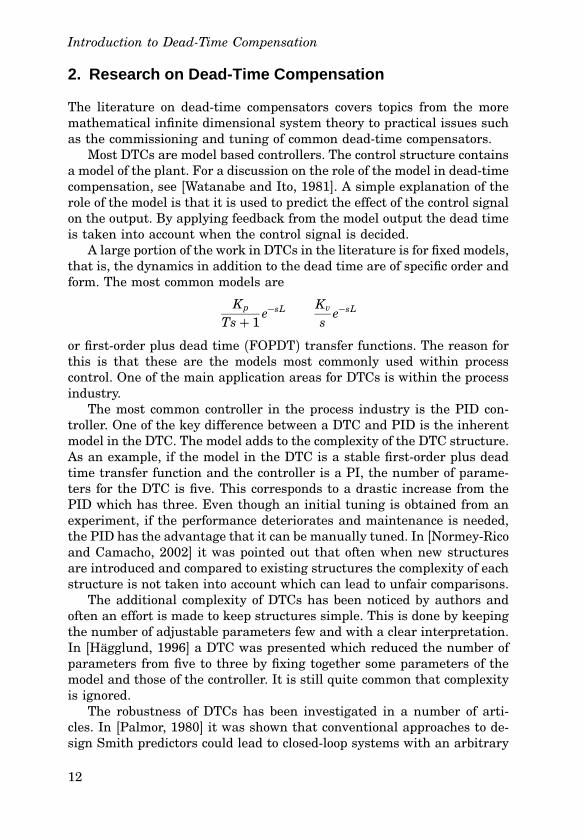
A large portion of the work in DTCs in the literature is for fixed models,that is, the dynamics in addition to the dead time are of specific order andform. The most common models are
Kp
Ts+ 1e−sL Kv
se−sL
or first-order plus dead time (FOPDT) transfer functions. The reason forthis is that these are the models most commonly used within processcontrol. One of the main application areas for DTCs is within the processindustry.
The most common controller in the process industry is the PID con-troller. One of the key difference between a DTC and PID is the inherentmodel in the DTC. The model adds to the complexity of the DTC structure.As an example, if the model in the DTC is a stable first-order plus deadtime transfer function and the controller is a PI, the number of parame-ters for the DTC is five. This corresponds to a drastic increase from thePID which has three. Even though an initial tuning is obtained from anexperiment, if the performance deteriorates and maintenance is needed,the PID has the advantage that it can be manually tuned. In [Normey-Ricoand Camacho, 2002] it was pointed out that often when new structuresare introduced and compared to existing structures the complexity of eachstructure is not taken into account which can lead to unfair comparisons.
The additional complexity of DTCs has been noticed by authors andoften an effort is made to keep structures simple. This is done by keepingthe number of adjustable parameters few and with a clear interpretation.In [Hägglund, 1996] a DTC was presented which reduced the number ofparameters from five to three by fixing together some parameters of themodel and those of the controller. It is still quite common that complexityis ignored.
The robustness of DTCs has been investigated in a number of arti-cles. In [Palmor, 1980] it was shown that conventional approaches to de-sign Smith predictors could lead to closed-loop systems with an arbitrary
12

3. Outline and Summary of Contribution
small dead time margin. In [Laughlin et al., 1987] the robust performanceof Smith predictors was investigated. Conditions for robust performancewere presented for the stable FOPDT case assuming that each of thethree model parameters would lie in an interval. A very similar prob-lem was addressed in [Lee et al., 1996]. The robustness of the structurepresented in [Hägglund, 1996] was further investigated in [Normey-Ricoet al., 1997] and a new structure proposed. For a more theoretical ap-proach to the robustness problem see [Meinsma and Zwart, 2000] wherea mixed sensitivity H∞ problem is solved for a linear system with delay.
The Smith predictor does not yield zero steady state error to a loaddisturbance when the plant has an integrator. A dead-time compensa-tion structure which had this very desirable property even for integratingplants was presented in [Watanabe and Ito, 1981]. A number of publica-tions have followed and treated this problem. The solutions vary in com-plexity and disturbance rejection capability. Some references are [Åströmet al., 1994; Matausek and Micic, 1996; Matausek and Micic, 1999; Normey-Rico and Camacho, 1999].
3. Outline and Summary of Contribution
Paper 1
The first paper deals with tuning of simple dead-time compensators. TwoDTCs are considered, one for self regulating processes and one for inte-grating processes. The DTC structure for self regulating processes wasfirst presented in [Normey-Rico et al., 1997] but the parameters of thestructure are selected differently in the current work. The DTC for inte-grating processes is the one presented in [Matausek and Micic, 1996].
A new method to identify the first-order plus dead time models shownbefore, is presented. The identification procedure consists of two step re-sponses, one in closed loop and one in open. The design procedure for thetwo DTCs result in a first order set-point response, corresponding to themodel
1Trs+ 1
e−L
It is shown how a suitable lower bound on the closed-loop time constant,Tr, can be found by considering the area between the plant output andthe model output when a step is applied to both. In the integrating caseit is actually two steps, one up and one down, to limit the change in theplant output. It is also shown how dead time margin depends on Tr.
13
Introduction to Dead-Time Compensation
Paper 2
A common sight in the literature is an introduction of a new structurewhich is shown to outperform other structures in a few simulation exam-ples. Robustness is frequently not taken into account in the comparisoneven though it is well known that a robustness/performance tradeoff isalways present in controller design.
The second paper is concerned with the use of DTCs or more specifi-cally, when they should be used. Recognizing that the control strategy thatthe DTC probably would replace would be a PI or PID, the performanceof the DTC is compared to that of PI(D) under a robustness constraint.Typical DTCs for both stable and integrating processes are compared tothe best PI and PID which fulfill the robustness constraint.
14
Paper 1
Robust tuning procedures ofdead-time compensating controllers
Ari Ingimundarson and Tore Hägglund
Abstract
This paper describes tuning procedures for dead-time compensat-ing controllers (DTC). Both stable and integrating processes are con-sidered. Simple experiments are performed to obtain process modelsas well as bounds on the allowable bandwidth for stability. The DTCsused have few parameters with clear physical interpretation so thatmanual tuning is possible. Furthermore, it is shown how the DTCscan be made robust towards dead-time variations.
Keywords Automatic tuning, Dead-time compensation, Robustness,PID control
Reproduced with permission from: Ingimundarson, A. and T. Hägglund(2001): “Robust tuning procedures of dead-time compensating
controllers”, Control Engineering Practice 9, p.1195-1208.
15

Paper 1. Robust tuning procedures of dead-time compensating controllers
1. Introduction
Most control problems in the process industry are solved using PID con-trollers. There are several reasons for this. One is that the PID controllercan be tuned manually by “trial-and-error” procedures, since it only hasthree adjustable parameters. The possibility to make manual adjustmentsof the controller parameters is important even when automatic tuningprocedures are available.
When there are long dead times in the process, the control performanceobtained with a PID controller is, however, limited. For these processes,dead-time compensating controllers (DTCs)may improve the performanceconsiderably. These controllers require a process model to provide model-predictive control. This usually means a significant increase in controllerparameters.
The use of DTCs also brings into existence new robustness problemsconnected to the dead-time. The classical ways to characterize robustness,phase margin and amplitude margin are not sufficient. In this paper, thedelay margin which is the greatest variation in dead time that can occurin the process before the closed-loop system becomes unstable, will beused as well.
The aim of this paper is to show how it is possible with simple ex-periments to find parameters for the DTCs that give good performancewhile remaining robust. The experiments are composed of an identifica-tion of simple process models and then an experiment to determine anupper limit on closed-loop bandwidth. The latter is performed in openloop while the former is partially performed in closed loop. As a measureof closed-loop bandwidth, the reciprocal of the time constant of the setpoint response is used. This can then be related to other measures suchas the loop-gain crossover frequency. The DTCs used in this paper havecertain PID qualities, i.e. few parameters that can be tuned manually andhave good interpretation in terms of classical control theory concepts. Itwill also be shown how the DTCs can be given a guaranteed delay margin.
For the identification of the simple process models in the DTCs anidentification method first presented in [Ingimundarson and Hägglund,2000a] is used. In this paper only the main equations and results arepresented.
The paper is arranged in the following manner. In Section 2 the identi-fication method is introduced. In Section 3, dead-time compensating con-trollers are discussed. In Section 4 the tuning procedure for stable pro-cesses is presented. This is followed by the procedures for integratingprocesses in Section 5. Finally conclusions are drawn in Section 6.
16

2. Identification
2. Identification
The two processes that are identified are the first-order plus dead time(FOPDT)
Pn(s) = Kn
Tns+ 1e−Lns (1)
and the two-parameter model
Pn(s) = Kn
se−Lns (2)
These models are frequently used in the process industry and are consid-ered to capture dynamics of real plants sufficiently well for many appli-cations.
The identification method presented in this paper can be divided intotwo phases. First, the average residence time, Tar = Ln+Tn and the gainKn are estimated with a change in operating levels. This change can beaccomplished by a change in set point while operating in closed loop. Theapproach is based on the method of moments, see [Åström and Hägglund,1995] for a general input signal applied to a linear system initially at rest.Second, the apparent time constant Tn is determined with an open-loopexperiment where the input signal is a step or a ramp. In the case of thetwo-parameter model given by Eq. (2) only the first part of the experimentis necessary.
The method of moments
The method of moments can be explained with the following equations.For a general transfer function G(s) an arbitrary input signal U(s) resultsin an output signal given by
Y(s) = G(s)U(s) (3)
By derivating Y(s) with regard to s one gets
Y ′(s) = G′(s)U(s) + G(s)U ′(s) (4)
The transfer function G(s) and its derivative can be evaluated at an ar-bitrary point α by calculating
Y(m)(α ) = (−1)m ∫∞0 tm e−α t y(t)dt
U (m)(α ) = (−1)m ∫∞0 tm e−α tu(t)dt
and solving Eqs. (3) and (4). Notice that if α = 0 it is necessary for thesignals considered to go to zero as time goes to infinity. Otherwise, the
17

Paper 1. Robust tuning procedures of dead-time compensating controllers
integrals will not converge. Typically an input signal of the sort u(t) =u(∞)−u(t) is selected. u(∞) is the value of the input signal after steadystate has been reached again. The corresponding output signal is theny(t) = y(∞)− y(t). Then it is only necessary to integrate for a finite timeinterval. This interval is denoted [tb, t f ] in the following.
In the case of the FOPDT model, (Eq. (1)) it is easy to get the followingexpression
P′n(s)Pn(s) = −Ln − Tn
1+ Tns
By evaluating the transfer function at α = 0, Tar can be written as
Tar = −P′n(0)Pn(0) (5)
To evaluate P′n(0) it would be necessary to calculate the first moment ofy(t) and u(t) for signals for which the integrals converge. These integralshave bad noise properties because of the factor t. Values at the end of theexperiment have much higher weight than the ones in the beginning ofthe experiment. Therefore it is beneficial to consider the artificial signals
yd(t) = ddt y(t)
ud(t) = ddt u(t)
The novelty of the method is the use of these signals. Denoting the mthmoment of yd and ud with ym and um respectively, it is possible to evaluateP′n(0) as
P′n(0) =y1 − Pn(0)u1
u0(6)
Evaluating the moment integrals y0 and y1 gives
y0 =∫ ∞
0yd(t)dt = [ y(t)]∞0
= − y(0) (7)y1 = −
∫ ∞
0tyd(t)dt
= − [t y(t)]∞0 +∫ ∞
0y(t)dt
=∫ ∞
0y(t)dt (8)
18
2. Identification
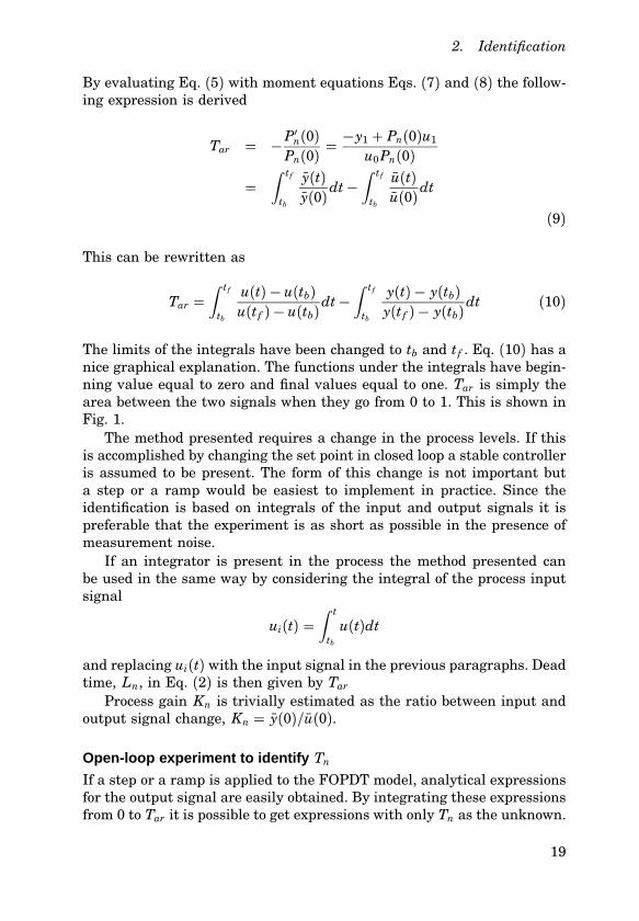
By evaluating Eq. (5) with moment equations Eqs. (7) and (8) the follow-ing expression is derived
Tar = −P′n(0)Pn(0) =
−y1 + Pn(0)u1
u0Pn(0)
=∫ t f
tb
y(t)y(0)dt−
∫ t f
tb
u(t)u(0)dt
(9)
This can be rewritten as
Tar =∫ t f
tb
u(t) − u(tb)u(t f ) − u(tb)dt−
∫ t f
tb
y(t) − y(tb)y(t f ) − y(tb)dt (10)
The limits of the integrals have been changed to tb and t f . Eq. (10) has anice graphical explanation. The functions under the integrals have begin-ning value equal to zero and final values equal to one. Tar is simply thearea between the two signals when they go from 0 to 1. This is shown inFig. 1.
The method presented requires a change in the process levels. If thisis accomplished by changing the set point in closed loop a stable controlleris assumed to be present. The form of this change is not important buta step or a ramp would be easiest to implement in practice. Since theidentification is based on integrals of the input and output signals it ispreferable that the experiment is as short as possible in the presence ofmeasurement noise.
If an integrator is present in the process the method presented canbe used in the same way by considering the integral of the process inputsignal
ui(t) =∫ t
tb
u(t)dt
and replacing ui(t) with the input signal in the previous paragraphs. Deadtime, Ln, in Eq. (2) is then given by Tar
Process gain Kn is trivially estimated as the ratio between input andoutput signal change, Kn = y(0)/u(0).
Open-loop experiment to identify Tn
If a step or a ramp is applied to the FOPDT model, analytical expressionsfor the output signal are easily obtained. By integrating these expressionsfrom 0 to Tar it is possible to get expressions with only Tn as the unknown.
19

Paper 1. Robust tuning procedures of dead-time compensating controllers
0
1
y(t)−y(tb)y(t f )−y(tb)
u(t)−u(tb)u(t f )−u(tb)
t ftb
Tar
Figure 1. Graphical explanation for Eq. (10)
In Eqs. (11) and (12) Tn is given for a step or ramp input signal.
Step : Tn = Ae1
hKn(11)
Ramp : Tn =√
AhKn(1/2− e−1) (12)
Parameter A is the integral of y(t) from 0 to Tar. The parameter h is theamplitude for a step signal or the rate for a ramp signal. The length ofthe open-loop experiment is always Tar.
Notice that Eq. (12) can be used for a FOPDT model with integratoras well. Sending a step of height h to an integrating process is the sameas sending a ramp with rate h to the process without an integrator. Inboth cases Eq. (12) can be used to find Tn. The problem with the open-loopramp experiment is that if the dead time Ln is sufficiently larger thantime constant Tn, one has to select a large h for a good signal to noiseratio in integral A. But after time Tar, y(t) will continue to rise since theprocess contains an integrator. Assuming that after time Tar precautionsare taken to reverse the direction of y(t) the maximum value of y(t), willstill be around hKnTar. This gives then an upper limit on rate h.
20

2. Identification
yb
y1 ← A
yf
tftb t f + Tar
ub
uf
u1
Figure 2. Identification experiment for G(s) = 1s+1 e−5s
Identification procedure
The basic steps in the identification procedure can now be presented. InFig. 2, the input and output signals are shown for a specific FOPDT pro-cess. For simplicity the change in set point for the closed-loop experimentis a step. The open-loop experiment is also a step.
1. Control the process to a steady state initial level yb. Record thesignal levels ub and yb.
2. Apply a step in the reference signal ysp(t) at time tb
3. Integrate y(t) and u(t) until process reaches steady state again. Thisoccurs at time t f . Again record the signal levels uf and yf .
4. Determine process gain Kn by observing the signal levels and Tar
from Eq. (10).5. Apply a step in open loop and integrate the area A using the estimate
of Tar obtained from previous step.
6. Estimate time constant Tn from Eq. (11) and dead time by Ln =Tar − Tn.
21
Paper 1. Robust tuning procedures of dead-time compensating controllers
Σ−
+
Σ+
ΣΣ
Σ
−
++
+
+
C(s) P(s)
Gn(s)
ysp yu
l
e−Lns
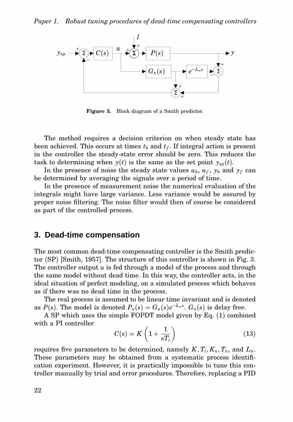
Figure 3. Block diagram of a Smith predictor.
The method requires a decision criterion on when steady state hasbeen achieved. This occurs at times tb and t f . If integral action is presentin the controller the steady-state error should be zero. This reduces thetask to determining when y(t) is the same as the set point ysp(t).
In the presence of noise the steady state values ub, uf , yb and yf canbe determined by averaging the signals over a period of time.
In the presence of measurement noise the numerical evaluation of theintegrals might have large variance. Less variance would be assured byproper noise filtering. The noise filter would then of course be consideredas part of the controlled process.
3. Dead-time compensation
The most common dead-time compensating controller is the Smith predic-tor (SP) [Smith, 1957]. The structure of this controller is shown in Fig. 3.The controller output u is fed through a model of the process and throughthe same model without dead time. In this way, the controller acts, in theideal situation of perfect modeling, on a simulated process which behavesas if there was no dead time in the process.
The real process is assumed to be linear time invariant and is denotedas P(s). The model is denoted Pn(s) = Gn(s)e−Lns. Gn(s) is delay free.
A SP which uses the simple FOPDT model given by Eq. (1) combinedwith a PI controller
C(s) = K(
1+ 1sTi
)(13)
requires five parameters to be determined, namely K , Ti, Kn, Tn, and Ln.These parameters may be obtained from a systematic process identifi-cation experiment. However, it is practically impossible to tune this con-troller manually by trial and error procedures. Therefore, replacing a PID
22

3. Dead-time compensation
controller with a standard SP gives a drastic increase in operational com-plexity. This increase is present in both the commissioning and mainte-nance of dead-time compensating controllers.
A common way to deal with this complexity is to automize the tun-ing procedure. Automatic tuning of DTCs has received some attention inthe literature, some references are [Palmor and Blau, 1994], [Lee et al.,1995] and [Vrancic et al., 1999]. But even when automatic tuning proce-dures are available simpler structures are advantageous since it providesa possibility for the user to make the last final adjustments manually ormanually retune the controller later.
A few papers have been written that emphasize the importance of lesscomplex DTCs. In the stable case, [Hägglund, 1996] is one example andin the case of integrating processes ,[Matausek and Micic, 1999] haveaddressed the problem.
The bandwidth of DTCs is usually related to the model parameterswhich are assumed to be available when the DTCs are initially tuned.In [Palmor and Blau, 1994], the closed-loop time constant was set pro-portional to the apparent dead-time of the process. In [Hägglund, 1996]it was related to the open-loop apparent time constant. In [Normey-Ricoet al., 1997] the closed-loop bandwidth was related to both of these.
In the case of integrating processes, it has been more common thatthe initial bandwidth is supposed to be manually tuned. Guidelines aregiven from where a starting point can be obtained. In [Normey-Rico andCamacho, 1999] the closed-loop time constant was related to an assumeddead-time error between the model and process. In [Matausek and Micic,1999] it was suggested that the closed-loop time constant should be setequal to the apparent time constant of the dynamics additional to theintegrator.
In this paper, a new approach is taken to determine the closed-looptime constant in the initial tuning. Given the model parameters it is pos-sible to calculate the uncertainty norm boundary of the DTCs. The uncer-tainty norm boundary tells how much the real process can deviate fromthe model at each frequency without the closed-loop system becoming un-stable. Then it is shown how it is possible with simple experiments toobtain frequency dependent inequalities bounding the model uncertainty.A lower bound on the closed-loop time constant is then found by mak-ing sure the model uncertainty found is always less than the uncertaintynorm boundary of the DTC’s. The goal is that this initial tuning is, whenthe model is close to the process, less conservative but robustly stable.
It was mentioned in the introduction that classical measures of ro-bustness such as gain and phase margin are not sufficient when dealingwith dead-time systems. This is discussed in [Palmor, 1980]. In additionto these classical ones it is proposed that a third one is used, namely the
23
Paper 1. Robust tuning procedures of dead-time compensating controllers
delay margin. The delay margin of a closed-loop system can be definedin the following way (modifying slightly the definition in [Landau et al.,1995]). If the Nyquist curve intersects the unit circle at frequencies ω i
with the corresponding phase margins Φi then the delay margin can bedefined as
DM = mini
Φi
ω i
Most of the tuning rules for DTCs presented in the literature providea certain delay margin. The initial tuning, which results from the pro-cedures in this paper, can have an arbitrary small delay margin if themodel describes the process well. Therefore, it is shown how the DTCscan be retuned with a guaranteed delay margin. This can have a practi-cal value when it is known how much the dead time might vary aroundthe operating point. Finally, it is also shown what delay margin can beexpected from the initial tuning in the nominal case, i.e., when the modeland process are equal.
4. Stable Case
In [Hägglund, 1996], a dead-time compensating controller with only threeadjustable parameters was presented. The controller can be viewed as aPI controller with model-based prediction. The abbreviation PPI standsfor “Predictive PI”. The controller can be tuned manually in the same wayas a PID controller.
The structure of the PPI controller is the same as for the Smith predic-tor, with the FOPDT model (1) combined with the PI controller (13). Theonly difference is the parameterization. The five adjustable parametersare reduced to three by introducing constraints between the controllerparameters and the model. These constraints are
Tn = Ti
Kn = κ /K(14)
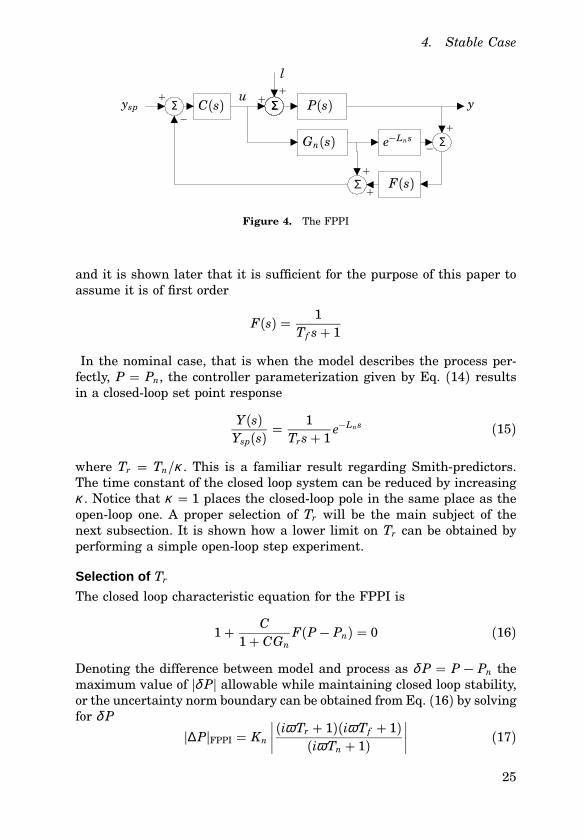
κ is a constant to be determined later. The identification method presentedbefore only provides a good approximation of the real process at low fre-quencies. Robustness problems for PPI can occur because of model errorat high frequencies. In [Normey-Rico et al., 1997] a filter was proposedto provide robustness towards high frequency model errors. The resultingcontroller was abbreviated FPPI. The proposed controller structure can beseen in Fig. 4. The filter F(s) is typically a one parameter low-pass filter
24
4. Stable Case
Σ−
+
Σ+
ΣΣ
Σ
−
++
+
+
C(s) P(s)
Gn(s)
ysp yu
l
e−Lns
F(s)
Figure 4. The FPPI
and it is shown later that it is sufficient for the purpose of this paper toassume it is of first order
F(s) = 1Tf s+ 1
In the nominal case, that is when the model describes the process per-fectly, P = Pn, the controller parameterization given by Eq. (14) resultsin a closed-loop set point response
Y(s)Ysp(s) =
1Trs+ 1
e−Lns (15)
where Tr = Tn/κ . This is a familiar result regarding Smith-predictors.The time constant of the closed loop system can be reduced by increasingκ . Notice that κ = 1 places the closed-loop pole in the same place as theopen-loop one. A proper selection of Tr will be the main subject of thenext subsection. It is shown how a lower limit on Tr can be obtained byperforming a simple open-loop step experiment.
Selection of Tr
The closed loop characteristic equation for the FPPI is
1+ C1+ CGn
F(P − Pn) = 0 (16)
Denoting the difference between model and process as δ P = P − Pn themaximum value of hδ Ph allowable while maintaining closed loop stability,or the uncertainty norm boundary can be obtained from Eq. (16) by solvingfor δ P
h∆PhFPPI = Kn
∣∣∣∣ (iω Tr + 1)(iω Tf + 1)(iω Tn + 1)
∣∣∣∣ (17)
25

Paper 1. Robust tuning procedures of dead-time compensating controllers
Notice that if an inequality of type
hδ Ph ≤ Aω (18)
is available the system can be made stable by chosing appropriately Tr
and Tf . This follows from the fact that the degree of the denominatorpolynomial is one higher than the numerator polynomial. The conditionfor stability would then be
hδ Ph ≤ Aω < h∆PhFPPI ∀ω (19)
An uncertainty bound of type (18) can be obtained with a simple open-loop step experiment. The step response of the real system is denoted byy(t). After an identification experiment the FOPDT model response isavailable and given by
yn(t) ={
0 for t < Ln
Kn(1− e−(t−Ln)/Tn) for t > Ln(20)
Denoting the difference between the two responses f (t) = y(t) − yn(t),the following expression is the definition of the Laplace transform
P(s) − Pn(s)s
=∫ ∞
0e−st f (t)dt (21)
Putting s = iω the following equation is obtained∣∣∣∣P(iω ) − Pn(iω )iω
∣∣∣∣ =∣∣∣∣∫ ∞
0e−iω t f (t)dt
∣∣∣∣≤
∫ ∞
0h f (t)hdt
= A (22)
Note that the error is weighted with one over ω . At stationarity there-fore there can be no error. Therefore Pn(s) and P(s) have to have the samesteady state gain Kn.
If a time constant Tf = A/Kn is defined the relevant areas can begraphically displayed on a normalized step response. This is shown inFig. 5.
Inequality (19) can now be restated the following way∥∥∥∥ Tf ω (iTnω + 1)(iTrω + 1)(iTf ω + 1)
∥∥∥∥∞< 1 (23)
26

4. Stable Case
0
1
Am
plit
ude
Time
Tn
Tf
Figure 5. Step responses y(t) and yn(t) normalized to 1.
Notice that Tf and Tn are assumed to be known while Tr and Tf are de-sign parameters. The latter two should be chosen to minimize some per-formance criteria while fulfilling the above inequality. For a fast set pointresponse, Tr could be chosen small while Tf would be used to fulfill theabove inequality. Commonly in process control, regulatory performance isconsidered more important. The performance criteria recommended hereis to minimize the integrated error when load disturbance l is a unit step.Using the final value theorem the following expression is obtained.∫ ∞
0e(t)dt = (Tr + Tf + Ln)Kn (24)
The design problem can be set up as a minimization problem where Eq.(24) is the cost function and Eq. (23) is the constraint. This problemcan be further simplified. Notice that Tr and Tf enter the cost functionand the constraint the same way. Using this fact it is possible to obtain
27

Paper 1. Robust tuning procedures of dead-time compensating controllers
necessary conditions that show that at the optimum, Tr is equal to Tf . Stillthe analytic solution to this problem quickly becomes rather involved. Anecessary condition for the constraint in Eq. (23) to be fulfilled is that thetransfer function has a direct term less than 1. This gives the followingcondition
Tr >√
TnTf (25)A further simplification of the problem can be obtained by normalizingthe frequency in inequality (23) with Tr. If the following quantities aredefined
ω = Trω γ = Tf /Tr
inequality (23) can be written as∥∥∥∥γ ω (iκω + 1)(iω + 1)2
∥∥∥∥∞< 1 (26)
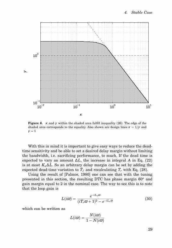
κ was defined following Eq. (15). Using a bisection algorithm, an upperlimit on κ for which inequality (26) holds, was calculated as a function ofγ . This is shown in Fig. 6. Any pair of κ and γ that lies within the shadesarea fulfills inequality (26). Using the above figure the following designrules are proposed
γ κ ≤ 1 γ ≤ 1 (27)In terms of the time constants this becomes
Tr ≥√
Tf Tn (28)Tr ≥ Tf (29)
Remark. The use of an equality in Eq. (28) requires justification. In-equality (22) allows infinite error when ω → ∞. Most normal processesare on the other hand of low-pass character. This means the inequal-ity could be replaced with a strict inequality at high frequencies. Whenκγ = 1 the supremum of the norm in Eq. (26) is achieved when ω →∞.So using additional information about inequality (22), Eq. (28) can bejustified.
Sensitivity to dead-time errors
Robustness of DTCs has been analyzed by many authors. Some referencesare [Morari and Zafiriou, 1989], [Palmor, 1980] and [Lee et al., 1996].Usually, most attention is devoted to analyzing the sensitivity towardserrors in the dead time. The reason for this is that it is often towardsthese errors dead-time compensators are most sensitive.
28
4. Stable Case
10−2
10−1
100
101
10−1
100
κ
γ
Figure 6. κ and γ within the shaded area fulfill inequality (26). The edge of theshaded area corresponds to the equality. Also shown are design lines κ = 1/γ andγ = 1
With this in mind it is important to give easy ways to reduce the dead-time sensitivity and be able to set a desired delay margin without limitingthe bandwidth, i.e. sacrificing performance, to much. If the dead time isexpected to vary an amount ∆L, the increase in integral A in Eq. (22)is at most Kn∆L. So an arbitrary delay margin can be set by adding theexpected dead-time variation to Tf and recalculating Tr with Eq. (28).
Using the result of [Palmor, 1980] one can see that with the tuningpresented in this section, the resulting DTC has phase margin 60o andgain margin equal to 2 in the nominal case. The way to see this is to notethat the loop gain is
L(iω ) = e−iLnω
(iTrω + 1)2 − e−iLnω (30)
which can be written as
L(iω ) = N(iω )1− N(iω )
29
Paper 1. Robust tuning procedures of dead-time compensating controllers
where N(iω ) is a frequency response with amplitude less than 1 for allω . Loop gain L(s) is always written as a function of a complex variableto distingish it from dead time L.
Further insight can be obtained into the relation between the delaymargin and closed-loop time constant Tr by normalizing the variables ofthe loop gain with Ln. This is the same approach as was taken in [Palmorand Blau, 1994]. If the process is equal to the model except for an errorin the dead-time, L = Ln + δ L, the loop gain becomes
L(s) = e−Ls
(Trs+ 1)2 − e−Lns (31)
If the variables are normalized with Ln the following dimensionless vari-ables are obtained.
δ L = δ L/Ln ω = ω Ln Tr = Tr/Ln (32)The normalized loop gain is then
L(iω ) = e−iω (1+δ L)
(iTrω + 1)2 − eiω (33)
The relationship between the two loop gains is L(iω Ln) = L(iω ). Byusing the Nyquist criterion it is possible to calculate a lower limit on Tr
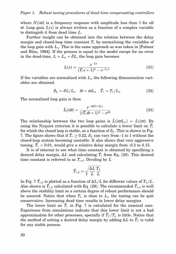
for which the closed loop is stable, as a function of δ L. This is shown in Fig.7. The figure shows that if Tr ≥ 0.22, δ L can vary from -1 to 1 without theclosed-loop system becoming unstable. It also shows that very aggressivetuning, Tr = 0.01, would give a relative delay margin from -0.2 to 0.15.
It is of interest to see what time constant is obtained by specifying adesired delay margin, ∆L and calculating Tr from Eq. (28). This desiredtime constant is referred to as Tr,d. Dividing by L
Tr,d =√
∆LL
Tn
L
In Fig. 7 Tr,d is plotted as a function of ∆L/L for different values of Tn/L.Also shown is Tr,d calculated with Eq. (29). The recommended Tr,d is wellabove the stability limit so a certain degree of robust performance shouldbe assured. Notice that when Tn is close to Ln the tuning can be quitconservative. Increasing dead time results in lower delay margins.
The lower limit on Tr in Fig. 7 is calculated for the nominal case.Experience from simulations indicate that this lower limit is not a badapproximation for other processes, specially if Tf /Tn is little. Notice thatthe method of setting a desired delay margin by adding ∆L to Tf is validfor any stable process.
30
4. Stable Case
−1 −0.5 0 0.5 10
0.05
0.1
0.15
0.2
0.25
0.3
0.35
0.4
0.45
0.5
δ L
Tr
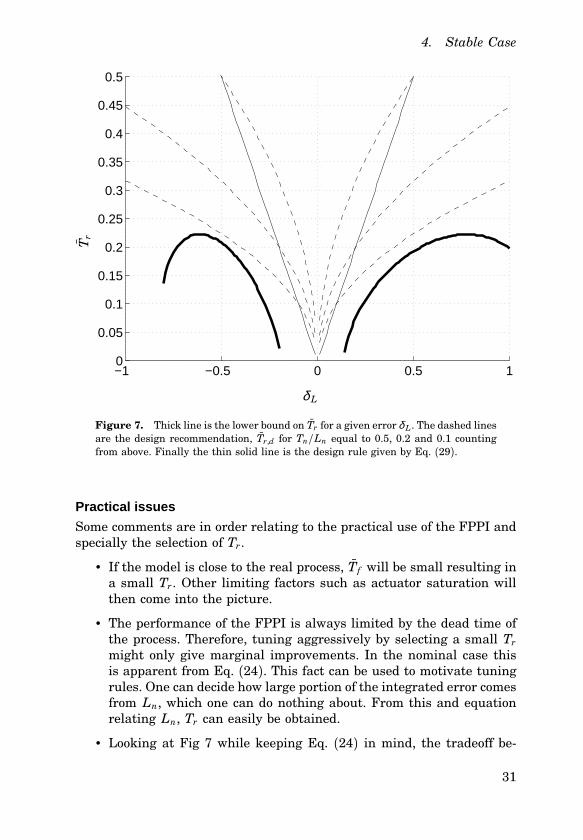
Figure 7. Thick line is the lower bound on Tr for a given error δ L. The dashed linesare the design recommendation, Tr,d for Tn/Ln equal to 0.5, 0.2 and 0.1 countingfrom above. Finally the thin solid line is the design rule given by Eq. (29).
Practical issues
Some comments are in order relating to the practical use of the FPPI andspecially the selection of Tr.
• If the model is close to the real process, Tf will be small resulting ina small Tr. Other limiting factors such as actuator saturation willthen come into the picture.
• The performance of the FPPI is always limited by the dead time ofthe process. Therefore, tuning aggressively by selecting a small Tr
might only give marginal improvements. In the nominal case thisis apparent from Eq. (24). This fact can be used to motivate tuningrules. One can decide how large portion of the integrated error comesfrom Ln, which one can do nothing about. From this and equationrelating Ln, Tr can easily be obtained.
• Looking at Fig 7 while keeping Eq. (24) in mind, the tradeoff be-
31

Paper 1. Robust tuning procedures of dead-time compensating controllers
Table 1. FOPDT model parameters as well as A and κ
i Tn Ln Tf Tr κ
1 10.4 6.8 0.27 1.7 6.2
2 2.0 6.2 0.27 0.7 2.7
3 3.0 9.1 1.06 1.8 1.7
4 1.7 8.4 1.18 1.4 1.2
5 0.8 5.4 0.17 0.4 2.4
6 7.6 2.6 1.32 3.2 2.4
7 1.3 5.7 0.17 0.5 2.7
tween performance and robustness is apparent. Robustness in termsof delay margin costs in terms of increased Tr.
Simulation examples
Simulation results for the PPI and the FPPI have been presented in [Häg-glund, 1996; Normey-Rico et al., 1997; Ingimundarson and Hägglund,2000b]. To give an idea of how conservative the design method presentedis, a FPPI controller was designed for a collection of processes. They areshown here without the dead time.
P1(s) = 1(10s+1)(2s+1) P2(s) = 1
(s+1)3P3(s) = −s+1
(s+1)5 P4(s) = −2s+1(s+1)3
P5(s) = 9(s+1)(s2+2s+9) P6 = 0.5
(s+1) + 0.05s+0.1
P7(s) = 64(s+1)(s+2)(s+4)(s+8)
The dead time was always equal to 5 making the total process equal to
P(s) = Pi(s)e−5s
for i ranging from 1 to 7.The results can be seen in Table 1. Notice that Tr is in all cases smaller
than Tn which means that the closed-loop system has a faster step set-point response than the open-loop one. Notice that the two processes withsmallest Tn/Tr ratio are non minimum phase and not monotonically de-creasing. Since the response goes in the wrong direction in the beginningthe area A becomes quite large in those cases. This reduces the bandwidththrough Tf .
32
4. Stable Case
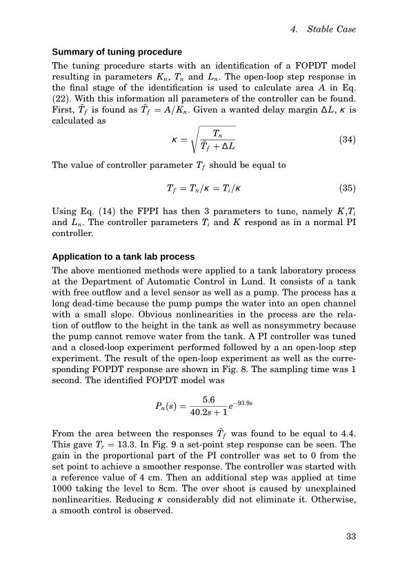
Summary of tuning procedure
The tuning procedure starts with an identification of a FOPDT modelresulting in parameters Kn, Tn and Ln. The open-loop step response inthe final stage of the identification is used to calculate area A in Eq.(22). With this information all parameters of the controller can be found.First, Tf is found as Tf = A/Kn. Given a wanted delay margin ∆L, κ iscalculated as
κ =√
Tn
Tf + ∆L(34)
The value of controller parameter Tf should be equal to
Tf = Tn/κ = Ti/κ (35)
Using Eq. (14) the FPPI has then 3 parameters to tune, namely K ,Ti
and Ln. The controller parameters Ti and K respond as in a normal PIcontroller.
Application to a tank lab process
The above mentioned methods were applied to a tank laboratory processat the Department of Automatic Control in Lund. It consists of a tankwith free outflow and a level sensor as well as a pump. The process has along dead-time because the pump pumps the water into an open channelwith a small slope. Obvious nonlinearities in the process are the rela-tion of outflow to the height in the tank as well as nonsymmetry becausethe pump cannot remove water from the tank. A PI controller was tunedand a closed-loop experiment performed followed by a an open-loop stepexperiment. The result of the open-loop experiment as well as the corre-sponding FOPDT response are shown in Fig. 8. The sampling time was 1second. The identified FOPDT model was
Pn(s) = 5.640.2s+ 1
e−93.9s
From the area between the responses Tf was found to be equal to 4.4.This gave Tr = 13.3. In Fig. 9 a set-point step response can be seen. Thegain in the proportional part of the PI controller was set to 0 from theset point to achieve a smoother response. The controller was started witha reference value of 4 cm. Then an additional step was applied at time1000 taking the level to 8cm. The over shoot is caused by unexplainednonlinearities. Reducing κ considerably did not eliminate it. Otherwise,a smooth control is observed.
33

Paper 1. Robust tuning procedures of dead-time compensating controllers
1000 1050 1100 1150 1200 1250 1300 1350 14003
4
5
6
7
8
9
Time [sec]
h[cm
]
Figure 8. Open loop step response of the real tank (solid line), and the model(dashed line).
200 400 600 800 1000 1200 1400 1600 1800 20000
2
4
6
8
10
200 400 600 800 1000 1200 1400 1600 1800 20000
1
2
3
Time [sec]
h[cm
]u[vo
lt]
Figure 9. Closed loop step response of the real tank with a FPPI controller.
34
5. Unstable case, integrating processes
Σ−
+
Σ+
ΣΣ
Σ
−
+
+
+
ΣΣΣΣ
+
−Kr P(s)
Gn(s)
ysp yu
l
e−Lns
F(s)
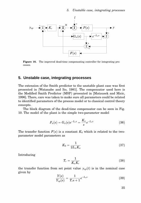
Figure 10. The improved dead-time compensating controller for integrating pro-cesses.
5. Unstable case, integrating processes
The extension of the Smith predictor to the unstable plant case was firstpresented in [Watanabe and Ito, 1981]. The compensator used here isthe Modified Smith Predictor (MSP) presented in [Matausek and Micic,1996]. There, care was taken to make sure all parameters could be relatedto identified parameters of the process model or to classical control theoryconcepts.
The block diagram of the dead-time compensator can be seen in Fig.10. The model of the plant is the simple two-parameter model
Pn(s) = Gn(s)e−Lns = Kn
se−Lns (36)
The transfer function F(s) is a constant K0 which is related to the two-parameter model parameters as
K0 = 12Ln Kn
(37)
Introducing
Tr = 1Kn Kr
(38)
the transfer function from set point value ysp(t) is in the nominal casegiven by
Y(s)Ysp(s) =
1Trs+ 1
e−Lns (39)
35

Paper 1. Robust tuning procedures of dead-time compensating controllers
Tr has therefore the nice interpretation of being the time constant fromset point to the output signal.
From the above equations it is clear that given a process model Pn(s)the only parameter left to determine is Tr. That is the subject of the nextsection.
Determining Tr
In [Normey-Rico and Camacho, 1999] a DTC for integrating processes wasproposed whose closed-loop time constant was related to asymptotes of theuncertainty norm-bound of the DTC. The same approach is taken here.
The error between the plant and the model is
δ P(s) = P(s) − Pn(s) (40)
The uncertainty norm-bound for the MSP or the maximum value of hδ Phallowed while keeping closed loop stability is
h∆PhMSP = hKn( jω Tr + 1)(2Ln jω + e− jLnω )hh − (2Ln + Tr)ω 2 + jω )h (41)
This equation is obtained from the characteristic equation in a similarway as Eq. (17).
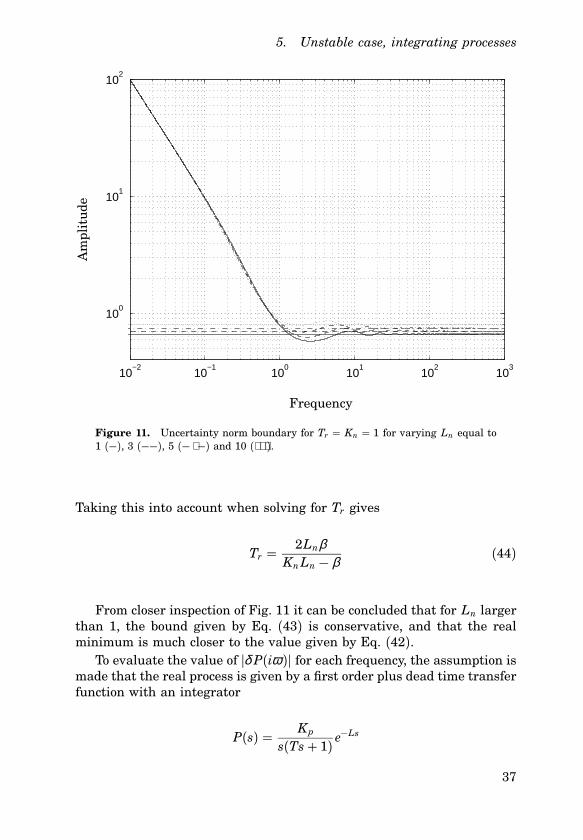
As pointed out in [Normey-Rico and Camacho, 1999] this bound de-pends almost entirely on Tr. The bound is shown in Fig. 11. For lowfrequencies the bound behaves as
h∆P(iω )h � Kn
ω
For high frequencies the bound has an asymptote given by
limω→∞ =
2Kn LnTr
2Ln + Tr(42)
To evaluate the minimum of the uncertainty norm-bound it is fruit-ful to consider it a product of two factors, one of which is monotonicallydecreasing. The one that has local minima is
f (ω ) =∣∣∣∣2 j Lnω + e− jLnω
ω
∣∣∣∣The minimum value of this function can be approximated with Ln. Thisgives a lower bound of h∆P(iω )h
β = Kn LnTr
2Ln + Tr≤ min
ωh∆P(iω )h (43)
36
5. Unstable case, integrating processes
10−2
10−1
100
101
102
103
100
101
102
Am
plit
ude
Frequency
Figure 11. Uncertainty norm boundary for Tr = Kn = 1 for varying Ln equal to1 (−), 3 (−−), 5 (− ⋅−) and 10 (⋅ ⋅ ⋅).
Taking this into account when solving for Tr gives
Tr = 2LnβKn Ln − β
(44)
From closer inspection of Fig. 11 it can be concluded that for Ln largerthan 1, the bound given by Eq. (43) is conservative, and that the realminimum is much closer to the value given by Eq. (42).
To evaluate the value of hδ P(iω )h for each frequency, the assumption ismade that the real process is given by a first order plus dead time transferfunction with an integrator
P(s) = Kp
s(Ts+ 1) e−Ls
37

Paper 1. Robust tuning procedures of dead-time compensating controllers
The absolute value of δ P(iω ) is then
hδ P(iω )h =∣∣∣∣Kpe−iLω − Kn(iTω + 1)e−iLnω
(iTω + 1)iω∣∣∣∣
As pointed out in [Normey-Rico and Camacho, 1999] this function can becharacterized by three main frequency intervals. For small ω this functionbehaves as
hδ P(iω )h �∣∣∣∣Kp − Kn
ω
∣∣∣∣For large ω this function has a slope of 20dB/dec. For sufficiently highand low frequencies hδ Ph will be smaller than h∆Ph. It is the error atintermediate frequencies that is of most interest. This will be referred toas δ P0 in the following.
In [Normey-Rico and Camacho, 1999] the value at intermediate fre-quencies was approximately calculated by assuming that the velocitygains of the model and process were equal, Kp = Kn. Then δ P0 couldbe estimated as
δ P0 = lims→0
δ P(s) = Kn(L + T − Ln) (45)
In [Normey-Rico and Camacho, 1999] δ P0 is viewed as a tuning parameterfrom which the closed-loop time constant is calculated. The methodologyis therefore to assume an error between L+T and Ln and from there getthe initial tuning.
Here the approach is to perform a simple open-loop experiment fromwhere a upper bound is found on δ P0. The area between the actual re-sponse and the response of the model is calculated when the input is animpulse of height hp and duration τ p. Denoting as before f (t) = y(t)−yn(t)the following equation is the definition of the Laplace transform.
δ P(s)hp(1− e−τ ps)s
=∫ ∞
0e−st f (t)dt (46)
From this equation, by replacing the argument s with iω the followinginequalities are obtained.∣∣∣∣δ P(iω )hp(1− e−τ piω )
iω
∣∣∣∣ =∣∣∣∣∫ ∞
0e−iω t f (t)dt
∣∣∣∣≤
∫ ∞
0h f (t)hdt
38

5. Unstable case, integrating processes
0
1A
mpl
itu
de
Time
A
Figure 12. The area A for the integrating case.
Notice that an upper bound on δ P0 can be obtained as
δ P0 ≤∫∞
0 h f (t)hdthpτ p
= A (47)
The area A has a nice graphical interpretation if the impulse response ofthe model and real process is normalized to 1 and plotted on the samegraph. A is then the area between the curves. This is shown in Fig. 12.
Notice that this bound on δ P0 is always larger and therefore more con-servative than the value obtained by Eq. (45). Since δ P(iω ) is weightedwith (1− e−iτ pω )/ω in the inequality, δ P(iω ) can be arbitrary large whenτ pω = 2π . The above method therefore does not guarantee stability butshould work well for well-behaving processes. The gain is that it elimi-nates the need to tune the last parameter. Substituting β with A in Eq.(44) gives then the time constant Tr.
39

Paper 1. Robust tuning procedures of dead-time compensating controllers
Sensitivity to dead-time errors
Given an error ∆L in the dead-time of the real process, the increase inintegral A would be maximum ∆LKn. Suspected variations in the deadtime can therefore be taken into account by increasing β in Eq. (44) by∆LKn.
If it is assumed that the process has the same structure as the modelbut a different dead time, L = Ln + δ L the loop gain of the MSP is
L(s) = 12
e−Ls((2Ln + Tr)s+ 1)sLn(Trs+ 1− e−Lns) (48)
Using the same approach as in the previous section the following dimen-sionless variables are defined
δ L = ∆L/Ln ω = ω Ln Tr = Tr/Ln (49)
This gives the following dimensionless loop gain
L(iω ) = 12
e−i(1+δ L)ω (i(2+ Tr)ω + 1)iω (iTrω + 1− eiω ) (50)
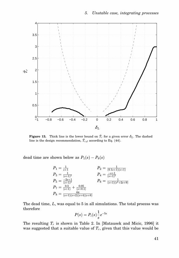
Fig. 13 shows the lower bound on Tr to maintain stability as a functionof δ L. The bound is not symmetric around 0. Rather it is shown that anincrease in dead time is more likely to cause instability than a decrease.If Tr is larger than 0.4 it will be stable for any decrease in δ L down to−1. For an initial tuning which would give Tr equal to 0.01, the controllerwould be stable for δ L ∈ [−0.22, 0.14].
The design rule given by Eq. (44) can be rewritten relating Tr to anassumed error ∆L by using β = ∆LKn. This results in
Tr,d = 2δ L
1− δ L(51)
This function is also shown in Fig. 13. The suggested Tr,d is well abovethe stability limit.
Simulation examples
To get an idea about what closed-loop time constant one can expect toobtain with the presented methodology, a two-parameter model was foundfor a collection of processes. The dynamics additional to the integrator and
40
5. Unstable case, integrating processes
−1 −0.8 −0.6 −0.4 −0.2 0 0.2 0.4 0.6 0.8 10
0.5
1
1.5
2
2.5
3
3.5
4
δ L
Tr
Figure 13. Thick line is the lower bound on Tr for a given error δ L. The dashedline is the design recommendation, Tr,d according to Eq. (44).
dead time are shown below as P1(s) − P8(s)
P1 = 1s+1 P2 = 1
(0.1s+1)(s+1)P3 = 1
(s+1)3 P4 = −s+1(s+1)5
P5 = −2s+1(s+1)3 P6 = 1
(s+1)(s2+2s+9)P7 = 0.5
(s+1) + 0.05(s+0.1)
P8 = 64(s+1)(s+2)(s+4)(s+8)
The dead time, L, was equal to 5 in all simulations. The total process wastherefore
P(s) = Pi(s)1s e−5s
The resulting Tr is shown in Table 2. In [Matausek and Micic, 1996] itwas suggested that a suitable value of Tr, given that this value would be
41

Paper 1. Robust tuning procedures of dead-time compensating controllers
Table 2. Identification and tuning results for integrating processes.
i Tn Tr A Ln
1 1 0.8 0.4 6.0
2 1.0 0.8 0.4 6.1
3 2.0 2.1 0.9 8.0
4 3.0 2.8 1.2 11.0
5 1.7 3.2 1.4 10.0
6 0.8 0.7 0.3 6.2
7 7.6 21.5 5.3 10.6
8 1.3 1.1 0.5 6.9
available, could be the apparent time constant of the dynamics additionalto the integrator or Pi(s)e−5s. This is shown as well in the table as Tn.Notice that Ln is the dead time of the two-parameter model. ComparingTr and Tn one can see that usually they are quite close. Often Tr is a littlebit smaller than Tn. Exceptions to this are processes 5 and 7. Process 5 isnon-minimum phase while process 7 has a slow zero giving a large areaA compared to Tn. In the case of process 7, A is also very large comparedto Ln. This results in a large Tr according to Eq. (44).
Closed-loop set point and load disturbance responses are shown inFigs. 14 to 16 for a selection of processes when Tr is found from Eq. (44).The amplitude of the load disturbance was −0.03. Also shown (dashedline) are simulations when Tr is set equal to Tn.
Practical issues
Some remarks on the practical use of the methodology presented are inorder. Most of the remarks made in Section 4 apply here as well. Noticethat when A is close to Kn Ln, Tr becomes very large calculated with Eq.(44).
Extensions
In [Matausek and Micic, 1999] an extension to the MSP was proposed. Toimprove load disturbance rejection the transfer function F(s) should havethe form
F(s) = K0sTd + 1
sTd/10+ 1(52)
where Td = 0.4Ln and K0 = 0.6/(Ln Kn). The form of the transfer func-tion is similar to a PD controller. It’s purpose is also to predict the load
42

5. Unstable case, integrating processes
0 20 40 60 80 100 120
0
0.5
1
0 20 40 60 80 100 120−0.5
0
0.5
1
Time
uy
Figure 14. Simulation example. Process 3.
disturbances l better which in turn leads to better disturbance rejection.Simulation experience indicates it is possible to use this extension withthe tuning procedure presented. Sometimes the increase in conservative-ness associated with the procedure is welcomed. In Fig. 17 the Nyquistdiagram is shown for process 5 when Tr is found by the procedure pre-sented and as recommended in [Matausek and Micic, 1996]. It can be seenthat the latter results in an unstable closed-loop system.
Summary of tuning procedure
As in the stable case, the tuning procedure starts with an identificationexperiment which results in parameters Kn and Ln. K0 can then be foundfrom Eq. (37). Then, area A in Eq. (47) is found by performing an open-loop inpulse response on the process. If a delay margin ∆L is desired, itis added to A and then Tr is found from Eq. (44). Then Kr can be foundfrom Eq. (38).
43

Paper 1. Robust tuning procedures of dead-time compensating controllers
0 20 40 60 80 100 120
0
0.5
1
0 20 40 60 80 100 120−0.5
0
0.5
1
Time
uy
Figure 15. Simulation example. Process 5.
Application to a lab process
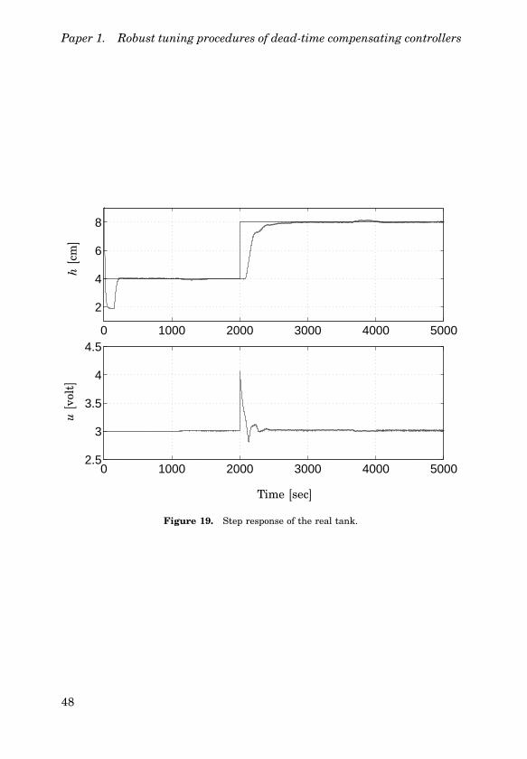
The method presented was used on the tank laboratory process presentedin Section 4 after some modification of the process. To make an integratingprocess a tank without an outflow hole was added under the first one.The controlled variable was therefore the height in the second tank. Toavoid nonlinearities at low flow levels, a second pump was installed whichpumped with a constant flow rate out of the lower tank. In this way thefirst pump was set to work around a constant flow rate corresponding to3 V.
The identification experiment was performed manually because it wasdifficult to tune a suitable PI controller. An impulse of height 1 Volt andduration 60 seconds was added to the equilibrium value of 3 Volts. Theresponse of the tank and the identified two-parameter model are shownin Fig. 18. The identified two-parameter model was
Pn(s) = 0.07s
e−132.5s
The area A between the responses was 1.6. This resulted in a closed-loop
44

6. Conclusions
0 20 40 60 80 100 120
0
0.5
1
0 20 40 60 80 100 120−0.5
0
0.5
1
Time
uy
Figure 16. Simulation example. Process 6.
time constant Tr = 54.8 seconds. In Fig. 19 a closed-loop step responseexperiment using the MSP is shown. The controller was started at time1000 while a step was applied at time 2000 taking the level in the tankfrom 4 cm to 8 cm. The controller performs as expected. The step responselooks similar to what was seen in simulation.
6. Conclusions
In this paper tuning procedures for dead-time compensators have beenpresented. Dead-time compensators for both stable and integrating pro-cesses are considered. The closed-loop time constant is found by comparingthe model output to the process output when a simple open-loop experi-ment is performed.
In the case of integrating processes the procedure eliminates the needto manually tuning one parameter.
The DTCs are simple and can be manually fine-tuned or re-tuned. Itis also shown how the DTCs can be given a guaranteed delay margin.
45

Paper 1. Robust tuning procedures of dead-time compensating controllers
−1 0 1 2 3 4−3
−2
−1
0
1
2
Figure 17. Nyquist curve for process 5, L = 10. Extended MSP with Tr foundfrom Eq. (44), (−). Extended MSP with Tr set equal to apparent time constant,Tr = 1.7, (−−).
Finally, the methodology has been applied to a laboratory process withsuccess.
46

6. Conclusions
0 50 100 150 200 250 300 350 4002
4
6
8
10
0 50 100 150 200 250 300 350 4002.5
3
3.5
4
4.5
Time [sec]
u[vo
lt]
h[cm
]
Figure 18. Identification experiment for integrating case. The upper graph showsthe impulse response of real tank (−) and that of the two-parameter model (−−).
47
Paper 1. Robust tuning procedures of dead-time compensating controllers
0 1000 2000 3000 4000 5000
2
4
6
8
0 1000 2000 3000 4000 50002.5
3
3.5
4
4.5
Time [sec]
u[vo
lt]
h[cm
]
Figure 19. Step response of the real tank.
48

Paper 2
Performance comparison betweenPID and dead-time compensating
controllers
Ari Ingimundarson and Tore Hägglund
Abstract
This paper is intended to answer the question: “When can a simpledead-time compensator be expected to perform better than a PID?”.The performance criterion used is the integrated absolute error (IAE).It is compared for PI and PID controllers and a simple dead-timecompensator (DTC) when a step load disturbance is applied at theplant input. Both stable and integrating processes are considered.For a fair comparison the controllers should provide equal robustnessin some sense. Here, as a measure of robustness, the H∞ norm ofthe sum of the absolute values of the sensitivity function and thecomplementary sensitivity function is used. Performance of the DTCsis given also as a function of dead-time margin (DM).
Keywords Performance Comparison, PID Control, Dead-time Com-pensators
Reprinted from: Ingimundarson, A. and T. Hägglund (2002):“Performance comparison between PID and dead-time compensating
controllers”, Journal of Process Control 12, p.887-895, with permissionfrom Elsevier Science.
49
Paper 2. Performance comparison between PID and DTCs
1. Introduction
In [Smith, 1957] a control structure was presented which became one ofthe main solutions to deal with processes with long dead time. Recently, arenewed interest in dead-time compensators has been noted in the controlliterature. Extensions to integrating and unstable processes have beenpresented, (see for example [Matausek and Micic, 1996] and [Majhi andAtherton, 2000]).
Despite this, little has been written about when DTCs should be used.Commonly in textbooks on process control a few pages are devoted toexplain the control structures of common DTCs but recommendations andguidelines about when to use DTCs are very rare.
The most common control structure in the process industry is the PI.The derivative gain is often turned off. This applies specially when longdead times are present. Therefore, given that the current control structureis a PI two options should be compared. One is to add the derivative partto the PI making it a PID. The other is to implement a DTC.
One reference where a similar comparison was done is [Rivera et al.,1986]. There, within the IMC framework, a PID controller was designedfor a first-order plus dead time (FOPDT) transfer function and comparedto best achievable performance of a DTC, that is when it has infinitegain. The performance criterion used was the Integrated Squared Error(ISE). DTCs with very high gains can have arbitrary small robustnesstoward dead-time errors, see [Palmor, 1980], even though their robustnessmeasured with traditional measures like amplitude margin, phase marginor maximum sensitivity, can be good. Therefore, in the current paper,performance of DTCs is given as a function of dead-time error sensitivity,measured with the dead-time margin (DM) or the smallest error in thedead time which causes instability. An other reference where the subject istreated is [Meyer et al., 1976]. There the robustness of the two structuresis not treated specially and the range of process dynamics for which thecomparison is made is small.
The layout of this paper is the following. The comparison criteria istreated in Section 2. The DTCs and their tuning is presented in Section3. In Section 4 the results are presented. This is followed by a discussionin Section 5. Finally conclusions are drawn in Section 6.
2. Comparison criteria
The purpose of this paper is to give insight into the problem of choosingbetween a DTC and a PI(D) within a typical process control environment.
50

2. Comparison criteria
While providing results general enough to be useful in that environment,certain assumptions are necessary to limit the size of the paper.
One question that arises is what information should be assumed to beavailable to select between control structures. Detailed knowledge can notbe assumed to be available since this is usually not the case within theprocess industry. In connection with the usage of DTCs, plants are oftenreferred to as being dead-time dominated. What is meant by this is thatthe ratio between dead-time and other dynamics is large and accordinglya decision to implement a DTC is taken. In this article it is assumed thatprocess information is available in terms of an first-order plus dead time(FOPDT) model, denoted with
P(s) = Kp
Ts+ 1e−Ls (1)
This is the simplest way to represent the division of process dynamics intopure dead-time, and other dynamics. In the case of integrating processesit is assumed that the FOPDT is in serial with an integrator
P(s) = Kp
s(Ts+ 1) e−Ls (2)
In the process industry, processes are commonly modeled with these trans-fer functions so most control engineers are familiar with their parame-ters. The comparison is made for these processes only. By making surecontrollers fulfill a robustness constraint, the results should be valid forplants sufficiently close to these models.
Another question that arises is the complexity of the controller struc-tures. The most commonly used structure in the process industry is the PIwhich has 2 parameters. A more complex structure with more parametersmight show better performance but still it might never be implementedsince this requires more expertize and advanced maintenance than thePI. In this paper, an effort has been made to keep the DTCs as simpleas possible. The DTC structures considered all contain a model of theprocess. Most parameters are related to this model. When the plant isequal to the model, the set-point response is given by a FOPDT transferfunction with unit gain.
1Trs+ 1
e−Ls (3)
Tr is selected with dead-time sensitivity in mind. This applies to the stableand integrating plant case. The models and the tuning of the DTCs willbe introduced in Section 3.
Within the process industry regulatory performance is usually moreimportant that set-point response. Therefore, the performance criterion
51
Paper 2. Performance comparison between PID and DTCs
ΣΣΣ
u
n
y
l
C(s) P(s)
−1
Figure 1. Block diagram of disturbance signals.
used was the IAE when a step load disturbance is applied at the plantinput. This comparison was performed for the FOPDT model for a gridingof the interval
T ∈ [0.01, 10] (4)while L and Kp were kept equal to 1. This range includes “almost” puredead-time processes to “almost” dead-time free processes.
It should be pointed out that while the comparison made in this paperis for load disturbances only, the main strength of DTCs has on the otherhand been its set point response. Further more it should be pointed outthat it has been a subject of many papers to improve the load disturbanceresponse of DTCs. As was said before, the DTCs presented here are simpleand there is much room for improvement.
The block diagram of the loop is shown in Fig. 1. C(s) is the controllerwhile P(s) is the process to be controlled. l is the load disturbance affect-ing the system while n is the measurement noise. For a FOPDT modelon interval (4), the PI(D) with the lowest IAE and with equal or betterrobustness was compared to the IAE of the DTC with the tuning obtainedfrom the FOPDT model. The robustness condition will be introduced inthe next section.
Since the PI(D) controller parameters are only subject to a robustnessconstraint, the comparison presented is not dependent of a specific tuningrule of the PI(D).
Robustness constraints
Caution has to be shown when comparing performance of control struc-tures because of the ever present tradeoff between robustness and per-formance. The comparison should be made under the assumption thatrobustness of the control structures is similar. A small deviation in theprocess should not result in a great difference in performance betweenthe structures.
The robustness measure used here is the H∞ norm of the sum ofthe absolute values of the sensitivity function and the complementary
52
2. Comparison criteria
sensitivity function
γ = supω(hS(iω )h + hT(iω )h) (5)
where
S = 11+ CP
T = CP1+ CP
(6)
This robustness measure or similar measures have appeared in variousplaces in the control literature. In [Panagopoulos and Åström, 2000] itwas shown how the Nyquist curve of a closed-loop system with a given γis guaranteed to stay out of the region given by the contours of
1+ hLhh1+ Lh = γ (7)
, L(s) is the loop gain, L(s) = C(s)P(s). Furthermore it was shown howthis parameter, with a suitable selection of weights for l and n is equiva-lent to the generalized robustness margin, see [Zhou, 1998].
In [Morari and Zafiriou, 1989] and [Doyle et al., 1992] the followingcondition for robust performance appears:
W1hS(iω )h +W2hT(iω )h < 1 ∀ ω (8)
For a typical process control problem the weights W1 and W2 should have aspecial shape. Weight W1 should be large at low frequencies to assure goodload-disturbance rejection. Weight W2 usually increases with frequencyto guarantee robustness toward model perturbations at high frequencies.The larger W1 can be, the better disturbance rejection. Larger W2 meansbetter robustness toward multiplicative uncertainties is assured.
The control structures presented in this article have certain inheritedqualities. All of them have infinite gain at low frequencies resulting inasymptotic rejection of a step load disturbance. In the nominal case it canbe shown with simple analysis that hS(iω )h → 0 as ω when ω → 0. At highfrequencies the controllers have constant gain which means hT(iω )h → 0as 1/ω when ω →∞. Given two controllers with these qualities and equalγ there is a pair of weights, W1 and W2, such that condition (8) is fulfilledfor both controllers. These weights can be constructed by choosing themto be 1/γ for the frequency for which the supremum is achieved in Eq.(5). For other frequencies, W1 would be put equal to the smaller value ofh1/S(iω )h for the two controllers. W2 would be chosen similarly to be thesmaller value of h1/T(iω )h. The implication of this is that there is a setof plants, around the nominal one, for which both controllers satisfy therobust performance condition given by Eq. (8).
53

Paper 2. Performance comparison between PID and DTCs
Σ−
+
Σ+
ΣΣ
Σ
−
++
+
+
Cc(s) P(s)
G0(s)
ysp yu
l
e−Ls
Figure 2. Block diagram of the simple DTC.
Dead-time sensitivity
A useful concept when dealing with DTCs is the dead-time margin (DM )or the smallest change in the dead time which will cause instability. Therobustness measure presented in the previous chapter does not capturedead-time sensitivity of DTCs. The reason is that it is caused by largeloop gain in the right-half plane of the Nyquist diagram, see [Åström andHägglund, 2001; Palmor and Blau, 1994], while the robustness measureis related to regions on the left side of the Nyquist diagram. Dead-timesensitivity can be taken into account by proper tuning of the DTCs. Thegeneral principle in this article was to select a tuning so that the ampli-tude of the loop gain was strictly smaller than 1 for frequencies larger thanthe crossover frequency, ω c (smallest frequency where hC(iω )P(iω )h = 1).
3. Controllers
Stable case
The block diagram for the DTC can be seen in Fig. 2. P(s) is the realprocess to be controlled. P0(s) is the model of the process with dead time,G0(s) is the model without. This way the controller for the DTC as indi-cated by Fig. 1 can be written as
C(s) = Cc(s)1+ Cc(s)G0(s)(1− e−Ls) (9)
The model P0(s) was the FOPDT model given by Eq. (1) and Cc(s) was aPI controller set to
Cc(s) = 1Trs
G−10 (s) =
Ts+ 1Tr Kps
(10)
54

3. Controllers
where Tr is a design parameter. This parametrization is related to H2
optimal control. The actual criteria it minimizes is the integrated squarederror (ISE) but because of its simplicity it is used even here. For referencesabout this parametrization, see [Laughlin et al., 1987].
In the nominal case, when there is no model error, P0(s) = P(s), thenTr is the time constant from set point ysp to output y.
Y(s)Ysp(s) =
1Trs+ 1
e−Ls (11)
Furthermore, the loop gain L(s) = C(s)P(s) is then given by
L(s) = e−Ls
Trs+ 1− e−Ls (12)
The robustness properties of this structure were analyzed in [Palmor andBlau, 1994]. There it was shown that L(iω ) never has a real part smallerthan −1/2. This means the phase margin and amplitude margin are min-imum 60o and 2 respectively. It was also shown how the dead-time margindepends on Tr/L. Some values are given in Table 1. For Tr/L ≥ 0.34 thedead-time margin is larger than 100%. This was the value used for thecomparison. Again, for this value the amplitude of the loop gain is alwaysless than 1 for frequencies larger than the crossover frequency.
In the nominal case the transfer function from l to y is given by
y(s) = P0(s)(
1− e−Ls
Trs+ 1
)l(s) (13)
This is easily seen to have an over damped response if l is a step. Thismeans that the IAE is equal to the integrated error (IE) and an analyticalexpression can be obtained by a Taylor series expansion of the exponentin Eq. (13) and applying the final-value theorem. This gives
I AE = limt→∞
∫ ∞
0e(t)dt = lim
s→0s
S(s)s2 = Kp(Tr + L) (14)
Table 1. Dead time margin in percentage with the corresponding minimum Tr/L
DM % 5 15 25 35 >100
Tr/L 0.03 0.10 0.16 0.24 0.34
55

Paper 2. Performance comparison between PID and DTCs
Σ−
+
Σ+
ΣΣ
Σ
−
+
+
+ΣΣΣΣ
+
−Cc(s) P(s)
G0(s)
ysp yu
l
e−τ s
F(s)
Figure 3. The improved dead-time compensating controller for integrating pro-cesses.
For example a DTC with DM equal to 35% will have IAE from a step loaddisturbance equal to 1.24KpL. With a very high gain DTC, obtained byTr � 0, one could get close to I AE = KpL. That is the lower limit withthe presented tuning.
Notice also that even if the IAE is independent of T , the response isnot. With a large T , settling time will also be very large.
The Modified Smith Predictor, integrating case
DTCs for integrating plants have been presented by a number of authors,see for example [Matausek and Micic, 1999; Normey-Rico and Camacho,1999]. The one chosen for the comparison in this article is the one pre-sented in [Matausek and Micic, 1999], see Fig. 3.
Y(s)Ysp(s) =
1Trs+ 1
e−τ s (15)
The reason for this is that this structure is very simple and replacementfrom a PI should be straight forward. This structure is an improvement ofa structure presented in [Matausek and Micic, 1996] which will be consid-ered for comparison as well. Tuning of this structure has been presentedin [Ingimundarson and Hägglund, 2001]. These controllers in [Matausekand Micic, 1996] will be referred to as the MSP (modified Smith predictor)and the one in [Matausek and Micic, 1999] as the IMSP (improved MSP).
As with most DTCs, these controllers contain a model of the plant tobe controlled. This is the two-parameter model
P0(s) = G0(s)e−τ s = Kp
se−τ s (16)
56

3. Controllers
As was explained before, the comparison is made for the collection ofFOPDT models in serial with an integrator as given by Eqs. (2) and (4).A two-parameter model approximation of the model given by Eq. (2) wasobtained by putting τ = T + L
The equation for the controller according to Fig. 1 is
C = Cc + F + FCcG0
1+ Cc(G0 − P0) (17)
The transfer function F(s) is given by
F(s) =
1
2τ Kp: MSP
0.72τ Kp
0.4τ s+ 10.04τ s+ 1 : IMSP
(18)
Finally Cc is a constant given by
Kr = 1KnTr
(19)
where Tr is the time constant of the transfer function from set point inthe nominal case when P = P0,
Then the loop gain can be expressed as a function of only dead time τand the time constant from reference value to the output, Tr
L(s) = e−τ s(s+ F(s)Trs+ F(s)Kp)s(Trs+ 1− e−τ s) (20)
It can be seen that the loop gain depends only on the ratio Tr/τ andtherefore the DM as well. In accordance with the tuning of the DTC forstable processes, this ratio was chosen so that the amplitude of L(iω ) forfrequencies larger than the cross-over frequency would be strictly smallerthan 1. This gave Tr/τ = 0.534.
The tuning recommended in [Matausek and Micic, 1996] was to setTr equal to T in the model (2). This parameter setting is included in thesimulation study that follows. Notice though that when T is small thistuning can give arbitrary small DM .
The PID parametrization
The PID was parametrized on parallel form
C(s) = K(
1+ 1Tis
+ TdsTd/Ns+ 1
)(21)
57

Paper 2. Performance comparison between PID and DTCs
10−2
10−1
100
101
0
0.2
0.4
0.6
0.8
1
1.2
1.4
1.6
1.8
2IA
E
T/L
Figure 4. IAE results for the different control structures in the stable case.DTC(−),PI (−−), PID (⋅ − ⋅)
with N = 10. N is sometimes considered a tuning parameter in the studyof PID controllers. To limit the complexity of the PID controller it wasfixed to a typical value as recommended in textbooks on process control.For PI, Td was set to 0.
4. Results
Stable case
The main result of the paper for the stable case is shown in Fig 4. IAEis displayed for PI, PID and the DTC for different values of T/L. Theperformance of the DTC is only dependent on the Tr/L ratio determinedby the dead-time margin and it is therefore constant over the entire rangeof the T/L ratio.
58
4. Results
To simplify discussions the range of T/L is split into three regions.
Top region. T/L ∈ [5, 10]. Here the performance of the PI is betterthan the DTC. This is not unexpected since when L = 0 the poles of theclosed loop system can be placed arbitrarily with a PI controller. The PIDperforms best of the controller structures.
Middle region. T/L ∈ [0.1, 5]. In this region the performance of theDTC is better than the PI. The largest difference is when T/L � 1. Therethe reduction in IAE following a switch to a DTC is at least 25%.
For T/L < 1 the PID performance is similar to the DTC. To obtain aDTC with better performance than a PID, it would have to be tuned moreaggressively with lower DM .
Bottom region. T/L = [0.01, 0.1]. The PI has higher IAE over theregion but the performance is quite similar. Notice that the performancecurve for the PI is leveling out and approaching a constant value as theFOPDT process approaches a pure dead-time process. Only a DTC withsmaller DM would have superior performance in this interval.
The performance of the PID approaches the performance of the PIwhen the ratio is decreasing. Investigation of the derivative gain showedit approaches zero for smaller T/L.
Integrating Case
The results in the integrating case are shown in Fig. 5. As the IAE variesconsiderably over the T/L range the IAE of all control structures wasnormalized with the IAE of the IMSP with Tr/L = 0.534.
The performance of the DTCs is better than the PI for all values ofT/L. Largest difference is for T/L � 3. There the IAE of the PI is 3.3times larger than the IAE for the DTC. For small T , when the processapproaches a pure dead-time process with an integrator, the ratio of theIAE between PI and DTC approaches a constant value. The PI has around2.5 times higher IAE than the DTC in this case.
If the IMSP and MSP are tuned as recommended with Tr = T , theperformance depends strongly on T/L but is always superior to the PI.
The PID performs much better than the other structures for large T/L.This it not surprising since if L = 0 in Eq. (2) the poles of the closed-loopsystem can be placed arbitrarily with a PID. For small T/L the PID hasa performance very similar to the IMSP.
Sensitivity analysis
The PI(D) controllers were compared to the DTCs under the assumptionthat they fulfilled the robustness constraint in Eq. (5) for equal or less
59

Paper 2. Performance comparison between PID and DTCs
10−2
10−1
100
101
0
0.5
1
1.5
2
2.5
3
3.5
4
T/L
Figure 5. Results for the integrating case. What is shown is the IAE normalizedwith the IAE of IMSP with Tr/L = 0.534 (−), PI (−−), PID (−⋅),IMSP with Tr = T(⋅ ⋅ ⋅ upper),MSP with Tr = T (⋅ ⋅ ⋅ lower).
γ . Yet it is interesting to see how IAE changes when the true process isnot the same as the nominal model. As there are only three parameters,a sensitivity star was determined for each parameter, for the stable andintegrating case. This was done for T/L ratio equal to 1. The sensitivitystars show how IAE changes, relative to the IAE for the correct model, asa function of parameter variation.
Stable case In Fig 6. the Nyquist diagram is shown. Also shown, onthe left half plane is the γ contour (encircling -1). It can be seen that allcontrollers touch the contour meaning they all have equal γ . Notice thatthe PID seems to touch the contour in more than one place.
In Figs. 7 to 9 the sensitivity stars for the different parameters areshown. Notice that the scale for IAE change is different on each figure.Generally speaking one can say that none of the structures seemed signif-icantly more sensitive to parametric changes than the others. For varying
60

4. Results
−2.5 −2 −1.5 −1 −0.5 0 0.5 1 1.5 2−2
−1.5
−1
−0.5
0
0.5
1
1.5
Figure 6. Nyquist diagram for the stable case, T/L = 1. DTC (−), PI (−−), PID(⋅− ⋅)
Kp the surprising thing is the increase in IAE for the PI on the right side.Comparing the load disturbance responses, one can see that the damp-ing in the PI response decreases more as a function of ∆Kp, than for thePID and DTC. For varying T the behavior is rather good for all structureswhen the change is larger than −0.5. For smaller values, the performanceof the DTC and the PID increases very quickly before the loop becomesunstable (∆T < −0.65). The PI on the other hand remains stable with asmall increase in IAE on that portion of the interval. The PID is most sen-sitive toward change in dead time, L. The IAE increases for all structuresfor positive change in dead time.
Integrating case The dead-time compensator for the sensitivity studywas the IMSP with Tr/L = 0.543. The Nyquist diagram for the integratingcase is shown in Fig. 10. Again all controllers lie tight up to the robustnessconstraint. The sensitivity stars are shown in Figs. 11 to 13. Again onecan say that no structure is significantly more sensitive than the others.
61

Paper 2. Performance comparison between PID and DTCs
−1 −0.5 0 0.5 1−20
0
20
40
60
80
100
120
∆Kp
%∆
IAE
Figure 7. Sensitivity star for K , stable case. DTC (−), PI (−−), PID (⋅− ⋅).
For a change in Kp it is obvious that the change in IAE for the DTC hasa dependence that is very close to linear in ∆Kp and the dependence isopposite to the other structures.
5. Discussion
There are many aspects that have not been considered in this comparison.The PID and DTC control structures each have advantages that should betaken into account. The PID is a well known structure frequently foundin distributed control systems as standard modules. One advantage of theDTC is that the dead time enters the control law directly, opening the pos-sibility for gain scheduling if the dead time is measurable. Furthermore,DTCs can be designed with certain dead-time margin if variations in thedead time are known, see [Ingimundarson and Hägglund, 2001].
An other aspect ignored here is the control signal amplitude or energy.
62
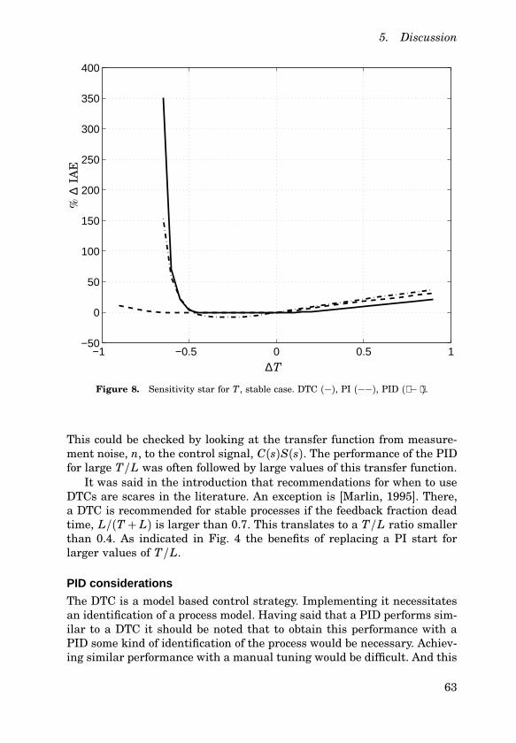
5. Discussion
−1 −0.5 0 0.5 1−50
0
50
100
150
200
250
300
350
400
∆T
%∆
IAE
Figure 8. Sensitivity star for T , stable case. DTC (−), PI (−−), PID (⋅− ⋅).
This could be checked by looking at the transfer function from measure-ment noise, n, to the control signal, C(s)S(s). The performance of the PIDfor large T/L was often followed by large values of this transfer function.
It was said in the introduction that recommendations for when to useDTCs are scares in the literature. An exception is [Marlin, 1995]. There,a DTC is recommended for stable processes if the feedback fraction deadtime, L/(T + L) is larger than 0.7. This translates to a T/L ratio smallerthan 0.4. As indicated in Fig. 4 the benefits of replacing a PI start forlarger values of T/L.
PID considerations
The DTC is a model based control strategy. Implementing it necessitatesan identification of a process model. Having said that a PID performs sim-ilar to a DTC it should be noted that to obtain this performance with aPID some kind of identification of the process would be necessary. Achiev-ing similar performance with a manual tuning would be difficult. And this
63

Paper 2. Performance comparison between PID and DTCs
−1 −0.5 0 0.5 1−100
0
100
200
300
400
500
600
∆L
%∆
IAE
Figure 9. Sensitivity star for L, stable case. DTC (−), PI (−−), PID (⋅− ⋅).
is not only due to the increase from two to three parameters. To supportthis claim, some contour lines in the PID parametric space is shown inFig. 14 for the integrating case when T/L = 1. For several values of Td
the contour lines in K and Ti are shown for the same γ as the IMSPhas when tuned with fixed Tr/τ ratio. It can be seen that the surface hassharp edges on it. Sharp edges of the parametric surfaces of PID’s hasbeen reported elsewhere, see [Åström and Hägglund, 2001]. To reach thisoptimal point by manual tuning might be difficult.
6. Conclusions
The paper has focused on comparing the performance of the PID controlstructure with simple DTCs. The purpose has been to gain insight aboutwhen each control structure should be used. IAE performance was deter-mined as a function of the ratio between time constant and dead time,T/L, for a collection of FOPDT models.
64

6. Conclusions
−2 −1.5 −1 −0.5 0 0.5 1−1.5
−1
−0.5
0
0.5
1
Figure 10. Nyquist diagram for the integrating case, T = 1. IMSP (−), PI (−−),PID (⋅− ⋅)
In the stable case, the main result is that for T/L in the interval[0.1, 5] a substantial decrease in IAE can be obtained by switching from aPI to a DTC. The performance of a PID is better than a DTC for T/L on[1, 10], otherwise it is similar to the DTC. A superior performance of theDTC on the interval [0.1, 1] could be obtained by accepting a smaller DM .
In the integrating case, the performance difference is much greaterbetween PI and the DTC. A switch to a DTC might reduce IAE to aboutone third of the IAE for PI. The PID performs best over a large portion ofthe area but it has been shown it might be difficult to obtain this optimalperformance with manual tuning.
65

Paper 2. Performance comparison between PID and DTCs
−1 −0.5 0 0.5 1−100
−50
0
50
100
150
200
250
300
∆Kp
%∆
IAE
Figure 11. Sensitivity star for K , integrating case. IMSP (−), PI (−−), PID (⋅− ⋅).
66
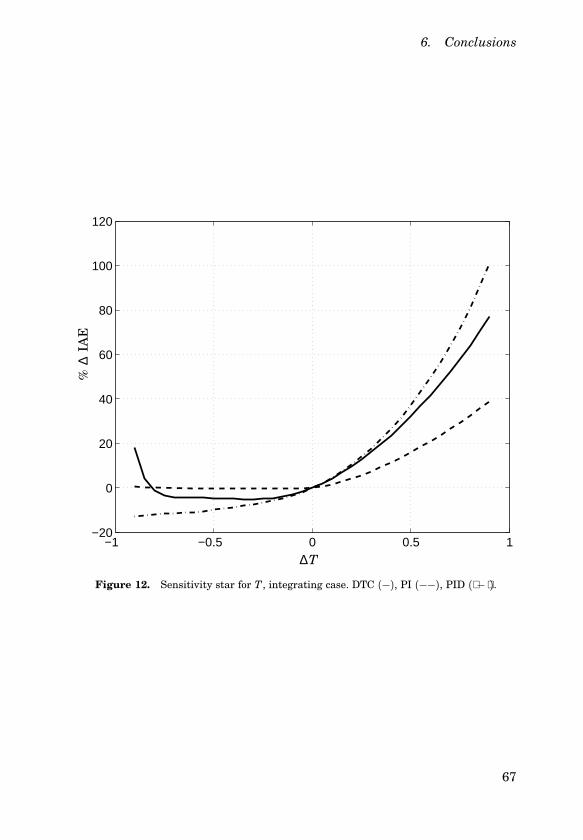
6. Conclusions
−1 −0.5 0 0.5 1−20
0
20
40
60
80
100
120
∆T
%∆
IAE
Figure 12. Sensitivity star for T , integrating case. DTC (−), PI (−−), PID (⋅− ⋅).
67

Paper 2. Performance comparison between PID and DTCs
−1 −0.5 0 0.5 1−100
0
100
200
300
400
500
∆L
%∆
IAE
Figure 13. Sensitivity star for L, integrating case. IMSP (−), PI (−−), PID (⋅− ⋅).
68
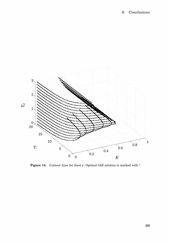
6. Conclusions
00.2
0.40.6
0.81
0
5
10
15
200
1
2
3
K
Ti
Td
Figure 14. Contour lines for fixed γ . Optimal IAE solution is marked with o.
69


Part II
Performance Monitoringof λ-Tuned Controllers


1
Introduction to PerformanceMonitoring
Much work has been done in the field of closed-loop performance monitor-ing and diagnostics (CLPM&D) in the last decade. This branch of auto-matic control research has matured enough so that a few survey articleshave appeared, see for example [Qin, 1998; Harris et al., 1999].
The purpose of the CLPM&D methods is to assist plant staff to in-terpret plant data. The goal is to run the plant as effectively as possible.The monitoring algorithm should sound an alarm when controllers arenot performing as expected. The diagnosis should give decision support tohelp with the overall maintenance of the closed loops in a plant.
The terms monitoring and assessment are used somewhat interchange-ably in the literature, usually referring to very similar algorithms. In thisthesis, what is meant with closed-loop performance monitoring is the ac-tion of watching for changes in a statistic reflecting performance over time.Assessment in this thesis refers to the action of assessing or evaluating astatistic that reflects performance at a certain point in time. The purposeof diagnosis is usually to determine the reason of poor performance. Thismight focus on one loop or a group of loops.
1.1 Control Performance in the Process Industry
Automated process control is an enabling technology to deal with thenatural variations of process variables from their desired values in a plant.The performance of a control system relates to its ability to deal with thisvariability.
The basic indication that something is wrong with a process is thatthe variability becomes too large. The deviation might be measured asvariance or standard deviation of the control error or estimated by visual
73

Chapter 1. Introduction to Performance Monitoring
inspection of process data. Operation targets are usually given in terms ofdeviation from set point, either as the absolute maximum or average overtime. There are many measures of variability, the one most often used inthis thesis is variance.
Numerous investigations have shown that performance of feedbackcontrollers is not good in the process industry, see [Bialkowski, 1993; En-der, 1993]. Typical numbers quoted are that 80% of loops have perfor-mance problems, 30% of loops actually increase variability in the shortterm over manual control.
This might be surprising in the light of the fact that about 95% offeedback controllers in the process industry are PI controllers. It is fairto say that with the amount of research effort put into control theory thelast decades, the problem of designing and commissioning PI controllers issolved. There are many ways to design good PI controllers but the problemis that the performance of a controller that once worked well is prone todegrade over time. Therefore, what is lacking is the maintenance of thecontroller after commissioning. Some of the reasons quoted for the lack ofmaintenance are
• Staff have limited time. The maintenance of controllers gets littletime, sometimes most of it is done on a “fire-fighting” basis. Onereason for the lack of time is that the operators have to many loopsto maintain.
• Lack of education and understanding of process control. Sometimesthe poor performance becomes the norm and people accept it asnormal.
The overall result is that companies are frequently not getting the bestpossible return on their investments into automated process control. Inlight of these facts the need for tools to assist staff to discover and fix pro-cess control problems is apparent. This need has generated a fair amountof research.
1.2 Why is Performance Poor?
There is a wide variety of reasons why loop performance might be poor.The equipment that the loop depends on can become faulty. Valves haveexcessive friction or stiction or they are not correctly dimensioned. In-put saturation breaks the feedback path temporarily. Varying transporta-tion times causes changes in dead time. The control structure or algo-rithm might be inappropriate. The controller might be badly tuned or dis-turbance characteristics for which the controller once was suitable have
74

1.3 Desired Properties of CLPM&D Methods
changed. The sampling time might be poorly selected. Finally, if a loophas performance problems, this might show up in neighboring loops.
This wide spectrum of root causes for performance deterioration hasgiven rise to a wide variety of methods to monitor and diagnose perfor-mance. There are a number of methods to monitor and diagnose oscil-lations, see [Horch, 2000; Hägglund, 1995]. Detection of sluggish controlloops has been treated in [Hägglund, 1999]. There are methods special-ized to diagnose valve problems such as stiction and backlash, see [Horch,2000].
Efficient diagnosis between root causes is a difficult problem. To imple-ment a number of methods and run them on-line in a distributed controlsystem (DCS)might be considered troublesome. An approach to this prob-lem is to have a performance monitoring algorithm running on-line whichdetects problem loops but does not distinguish between root causes. Thenthe root-cause diagnosis can be performed off-line. The performance mon-itoring algorithm presented in Chapter 3 is well suited as the algorithmrunning on-line.
The performance of feedback loops is subjected to limitations. Thesearise from plant dynamics such as dead time or right-half plane zeros.Saturation and dynamics of actuators pose limitations as do noise char-acteristics. This is important information when monitoring performance.Performance is hardly bad if it is close to what is optimally achievableconsidering the limitations. Even though it is close to optimal it mightstill not be acceptable. Many methods monitor performance by compar-ing the actual performance to the best achievable subjected to the knownlimitations. One of the main advantages of this approach is that only in-formation about the limitations is required. One of the disadvantage isthat there are many types of limitations and it is difficult to know themat all operating levels. Furthermore, performance far away from optimalperformance might be perfectly acceptable in some situations.
1.3 Desired Properties of CLPM&D Methods
In [Vaught and Tippet, 2001] a list of desirable properties a CLPM&Dmethod should have, was presented. Some of these properties are listedbelow and new ones have been added.
• Non-invasive. The method should not disturb normal operation ofthe loop. A few researchers have suggested methods where this con-dition is not fulfilled. For instance, in [Kendar and Cinar, 1997] apseudo random binary sequence is added to the reference to findthe sensitivity function and complementary sensitivity function. In
75
Chapter 1. Introduction to Performance Monitoring
[Gustafsson and Graebes, 1998] a method which uses an externalprobing signal to distinguish between performance changes due tosystem changes and disturbances was presented. In [Huang andShah, 1998] a dither excitation is used to identify a disturbancemodel which was then used to calculate achievable performance fora specific IMC design.
• Low error rate. False alarms occur when the algorithm signals badperformance eventhough the performance is actually good. Misseddetections are those situations when the algorithm should give alarmbut it doesn’t. Too many false alarms or missed detections result ina reduced or no use of the method. The problem is to characterizeexactly, in terms of the loop condition, when either will happen.
• Automated operation. The method should run with little or no man-ual intervention.
• No history. The method should result in an absolute measure ofperformance. It should not need to run for a time to be effective.Frequently the indices of today have to run for some time after com-missioning to create a “normal” operation level. Deviations from thislevel is then what is monitored. This means some time is required tostart using the indices. If the loop is changed in some way it mightbe necessary to repeat the startup procedure.
• No process information. One should need little knowledge of theprocess or the controller. The reason being that to obtain this infor-mation and keep it uppdated would be expensive.
• Implementation in the DCS. It is preferable that a method is imple-mented directly in the DCS since information about parameters andthe operating condition (auto/manual) usually resides there, see adiscussion in [Hägglund, 2002].
Tradeoffs
The desirable properties are not all attainable or realistic. An actual im-plementation of a CLPM&D method would mean a tradeoff between theseconditions. New methods should also be viewed with this in mind as well.Probably not all prefer the same set of characteristics in a method.
Performance monitoring is a form of data compression where raw plantdata is compressed to present information for plant staff for maintenancepurposes. As always when data is compressed, information is lost. Usuallywith an increase in information content an increase in complexity follows.To interpret more detailed information requires more knowledge.
76

1.4 The Following Chapters
1.4 The Following Chapters
In Chapter 2 a review of previous work is presented. Most emphasis willbe on the work on which the performance monitoring algorithm presentedin Chapter 3, is built. The main characteristics of the monitoring algo-rithm presented in Chapter 3, separating it from other methods, is thatspecifications about performance from the tuning phase are used to setall parameters of the monitoring algorithm. This should reduce the com-missioning time since no historical information is required to implementthe index. The drawback is that the tuning information is needed for thecommissioning. In Chapter 4 a method will be presented which estimatesa gradient of the variance with regard to a controller parameter. The pur-pose of this statistic is to assist with parameter adjustment of controllers.
77
2
Previous Work
2.1 Introduction
A short review of the literature will be given. Most emphasis will be put onwork related to λ-monitoring, the method presented in the next chapter,but other research directions are noted in the passing. Some notation willbe introduced as well. To begin with a short note on industrial practicethat has not received much academic attention will be presented.
Industrial Practice
Despite poor performance of controllers in the process industry mainte-nance of controllers has always taken place. Operation targets are spec-ified in terms of measures of variability such as variance or standarddeviation. The most basic trigger for maintenance is unacceptable vari-ability in the loop. To monitor some measure of variability is obviously offundamental importance for efficient operation. It is unlikely that main-tenance efforts will be devoted to a loop that fulfills its operation targetseven though the controller is performing badly according to some statistic.In this thesis variance is the main measure of variability.
A commonly used statistic for the overall performance of a controller isthe uptime or service factor. This is the portion of time spent in auto, thatis, the portion of the time the controller is on. [Kozub, 2002] argues thatuptime will continue to be “the work horse” of performance monitoringsince low uptime is a sure signal that a loop needs maintenance.
To rely on variance alone as a measure of performance gives falsealarms regarding controller performance. The controller might be doingits job perfectly but still the variance might be unacceptable. With regardto uptime as a performance monitor it is noted in [Desbourough and Miller,2001] that high uptime does not mean good performance.
78

2.2 Academic Work
2.2 Academic Work
A rough classification of approaches to performance monitoring and di-agnosis presented in the literature is the following. Firstly, a number ofsingle number performance statistics, referred to as indices or potentials,have been suggested. The other approach can be explained as graphical in-spection of various functions, usually related to the controller error. Bothapproaches aim at compressing the complex plant data and presentingthe result to the operators. The first one is easier to automate, making ita more valuable “first indicator” of bad performance.
The method presented in this thesis is strictly SISO. Research intoperformance monitoring of multi-variable controllers has lagged behindthe SISO case but lately there has been much activity in this field. Ex-tensions from the SISO case where minimum variance performance iscompared to the actual performance has been advocated in [Harris et al.,1996; Huang et al., 1997]. An industrial perspective of the research isoffered in [Kozub, 2002].
An other problem receiving more attention is to diagnose which loopis responsible when bad performance is exhibited by a group of loops.Typically these disturbances are oscillatory. Some references dealing withthese problems are [Thornhill et al., 2002; Thornhill et al., 2001].
Most control problems in the process industry are solved using SISOcontrollers. To deal with interactions, loops are commonly configured withdifferent dynamics. The impact of well working “fast” loops on the “slower”loops should be small as their variability can be assumed to be of frequen-cies above the bandwidth of the “slower” loops. As the method presentedrelates to how well a controller fulfills the assumptions from the tuningstage, it should be useful to validate whether the assumptions about theconfigurations of dynamics hold.
Multi-variable controllers are considerably less frequent in the processindustry but their use is increasing considerably. Perhaps the advent ofmonitoring and diagnosis technology of these controllers will make theirimplementation feasible.
Performance Index Monitoring
Performance index monitoring refers to monitoring algorithms where asingle number reflecting performance is calculated repeatedly over timeand compared to an alarm limit. The alarm limit can be decided fromstatistical characteristics of the index or by some other criteria. One ofthe main advantage of this approach is that it is easy to automate.
An early reference based on this approach is [Devries and Wu, 1978].The index presented by Harris (see [Harris, 1989]) received much atten-tion and many improvements followed. The idea was to compare the vari-
79
Chapter 2. Previous Work
ance of the controller error to the minimum variance when the limitationto performance due to dead time are taken into account. The minimumvariance was found by identifying a time-series model of the error andsolving a Diophantine equation. The ratio of the minimum variance andthe actual variance has been called the Harris index in the literature.
Time-series modeling continued to be a cornerstone of much of thework following after [Harris, 1989]. In [Desborough and Harris, 1992] analternative form of the Harris index was presented as well as approximateprobability distributions which are useful for designing alarm limits. Theindex presented in this thesis is based on this alternative form of theHarris index. Hence, a special attention will be devoted to the indicescalculated from time series.
Graphical Inspection
Some of the earliest mentioning of the idea of performance monitoring isin [Åström, 1967]. There it is pointed out that an assessment of how closethe performance of a controller is to the optimal one could be estimatedby calculating and inspecting the covariance function. Under minimumvariance control, the control error should be a moving average of order dwhere d is the pole-zero excess of the plant in discrete time. Calculatingthe covariance function of such a time series for arguments larger than dshould result in zero.
In [Kozub, 1997; Kozub, 2002], a function deemed easier to interpretthan the covariance function was the impulse response from an identifiedtime-series model of the control error. The value of the impulse responsefor graphical inspection is also pointed out in [Huang, 1999].
In [Stanfelj et al., 1993] the cross correlation function between mea-surable disturbances and controller error was suggested as a tool to de-termine influence of disturbances. Finally, different spectra have beenmentioned. An extension to the multi-variable case has been presented in[Seppala et al., 2002].
In [Kozub, 2002] it is noted that graphical interpretation of the impulseresponse requires a critical threshold of training for plant staff. Graphicalinspections take time and therefore they are not a solution to the problemof plant wide performance monitoring because of the limited time of plantstaff. They are an important part of the secondary tool set to be usedafter a more basic algorithm triggers the auditing of the loop. Use ofexpert systems to package the information and provide decision supporthas been presented in [Harris et al., 1996]. See [Paulonis and Cox, 2003]for an idea of large scale implementation of graphical methods.
80

2.3 Indices Calculated from Time-Series Models
ΣΣ
−C(q−1)
D(q−1)
w
P(q−1)r y
a
e u
Figure 2.1 Basic block diagram of closed-loop system.
2.3 Indices Calculated from Time-Series Models
A set of assumptions about the process and the disturbances are usuallymade when the indices are derived. The central one is that the controlerror, e(k) = r(k) − y(k), is a stochastic process resulting when a linearmodel is driven by white noise, see Fig. 2.1. The plant output is describedby
y(k) = P(q−1)u(k) +w(k) (2.1)where q−1 is the backward shift operator. P(q−1) is linear time invariantand can be written as
P(q−1) = Bu(q−1)Au(q−1)q−d
where the pole-zero excess is d. Notice that sometimes d is called deadtime while other times it is d− 1. Following [Harris, 1989] the dead timeis defined as d, the pole-zero excess. The controller is assumed to be onedegree of freedom
u(k) = C(q−1)(r(k) − y(k))The disturbance w(k) is thought to be generated by white noise a(k) fil-
tered through the disturbance model D(q−1). The transfer function D(q−1)therefore determines the character of the disturbance affecting the sys-tem. A common assumption is that it is of ARIMA type or
D(q−1) = Bw(q−1)∇l
Aw(q−1) ∇ = 11− q−1 (2.2)
81

Chapter 2. Previous Work
The dependence of the controller error on disturbance w(k) and the setpoint r(k) is given by the following equations
e(k) = r(k) − y(k)= 1
1+ C(q−1)P(q−1)(r(k) −w(k)) (2.3)
Notice that the way set point and the disturbance affect e(k) differs onlyby a sign.
Under regulatory control, r(k) is constant. For simplicity it can beassumed that e(k) has mean zero. Otherwise, it is the deviation from amean value which is modeled. For a treatment when the mean is notzero see [Desborough and Harris, 1992]. If r(k) is a stochastic process,by means of spectral factorization e(k) can be described by an ARMAtype linear model driven by a single white noise source. In this sectionregulatory control is assumed unless otherwise specified.
It is assumed that the data available for monitoring is
{r(k), y(k)} for k = 1 . . . N
or only at the latest time instant, k, for recursive implementation, seeFig. 2.1. This allows us to calculate the error, e(k) = r(k) − y(k).
Assuming that the plant and the disturbance model are not known,given e(k), a time-series model can be identified giving valuable informa-tion about the characteristics of the closed-loop system and the distur-bances affecting it. The identified time-series model is denoted
e(k) = B(q−1)A(q−1) a(k) (2.4)
Deterministic Disturbances
Notice that deterministic disturbances can be modeled in the same frame-work by assuming a(k) is zero except at isolated points in time. Dis-turbance scenarios more common in process control can then be takeninto account with assumptions on the disturbance model D(q−1). WhenD(q−1) = P(q−1)∇ then the disturbance will be referred to as a load dis-turbance. If D(q−1) = ∇ then it will be referred to as step disturbance.Since the disturbance w affects the error in the same way as r, a stepdisturbance can be attributed to a change in set point or a step change inw(k).
82

2.3 Indices Calculated from Time-Series Models
The Impulse Response
A useful and informative representation of the time series is the impulseresponse. It can be obtained by a series expansion in q−1, of the time-seriesmodel in Eq. (2.4). The equation can then be written as
e(k) =∞∑
j=0
f j q− ja(k) (2.5)
The first coefficient of the impulse response, f0, is often normalized tobe equal to 1. The variance of e(k) can be expressed with the impulseresponse as
σ 2e = var(e(k)) =
∞∑j=0
f 2j σ 2
a (2.6)
Considering Eqs. (2.5) and (2.6) together the subscript of the impulseresponse coefficients gives an idea from what time the contributions to thevariance come from. The impulse response coefficients f j can be plottedas a function of j. For finite variance it is clear that f j go to zero with j.A plot gives therefore an idea on how fast disturbances are rejected. In[Tyler and Morari, 1996] the relation of impulse response coefficients tocommon performance specifications is shown.
The pole excess d places a limit on how fast a controller can rejectdisturbances. The effect of a disturbance acting at time k will be reactedon earliest at time k+ d. The controller that manages to cancel the noiseperfectly as soon as it can is called a minimum variance (MV) controller,see [Åström, 1970]. To calculate the MV controller, full information aboutthe disturbances and the plant is required. Under MV control the errore(k) is a moving average given by the first d terms of the impulse responsewhich the controller can not affect. The variance of e(k) under MV control,denoted σ 2
M V is therefore
σ 2M V = (1+ f 2
1 + ⋅ ⋅ ⋅+ f 2d−1)σ 2
a
The Harris Index
It was noted in the introduction that variance alone is a poor indicationon how well the controller is doing. The problem is that the variance asan absolute statistic is not very informative. It has to be compared withsomething.
Harris noted that to assess control performance the variance of e(k)could be compared with the MV performance, σ 2
M V . This would be moreinformative on how well the loop was actually doing. If variance of e(k)is close to σ 2
M V , better performance can only be obtained by changing the
83

Chapter 2. Previous Work
f j
t∑d−1j=0 f 2
j∑∞
j=d f 2j
0 d−1 d
Figure 2.2 An impulse response to show the impulse response coefficients usedto calculate the Harris index.
process since σ 2M V is invariant to feedback. An index of performance could
therefore be calculated as the ratio between σ 2M V and σ 2
e .Harris also showed that a time-series model identified from e(k) could
serve to find σ 2M V . As the first d terms of the impulse response are in-
variant to feedback they should be equal in the actual system and theidentified time series model. A number of single number monitoring algo-rithms followed the work of Harris.
It was noted in the introduction that a graphical inspection of the im-pulse response is considered to be one of the most informative performanceinspections that can be done on data. Most of the indices calculated fromtime-series models can be thought to be attempts to automate graphicalinspections. The Harris index, for example, can be written as
I =∑d−1
j=0 f 2j∑∞
j=0 f 2j
(2.7)
It compares the sum of the d first impulse response coefficients squaredto the total sum, see Fig. 2.2.
The Normalized Performance Index
In [Desborough and Harris, 1992] the normalized performance index wasintroduced. It extended ideas presented in [Harris, 1989] by giving an al-ternative way of estimating an index related to the Harris index. Assumethat a predictor is created to predict b steps into the future for the timeseries in Eq. (2.4). The best predictor in the mean square sense will bea linear predictor, see [Åström and Wittenmark, 1997]. The predictor can
84

2.3 Indices Calculated from Time-Series Models
be obtained by solving a Diophantine equation or equivalently by longdivision of B(q−1) by A(q−1).
B(q−1) = A(q−1)F(q−1) + q−bG(q−1) (2.8)
q−bG(q) is the remainder of the division while F(q) is the quotient. Thepolynomial F(q) is also equal to the first b terms of the impulse responsein Eq.(2.5). The predictor is then given by
e(khk− b) = G(q−1)B(q−1) e(k− b) (2.9)
The variance of the prediction error, ε b(k) = e(k) − e(khk− b), is
var(ε b(k)) = (1+ f 21 + ⋅ ⋅ ⋅+ f 2
b−1)σ 2a (2.10)
where σ 2a is the variance of the noise a(k).
Notice that when a(k) is a deterministic disturbance, the predictor isfound by solving Eq. (2.8) in the same way as when the disturbance isstochastic, see [Åström and Wittenmark, 1997]. The expression to calcu-late the normalized performance index is the following
η(b) = 1− var(e(k) − e(khk− b))var(e(k)) = 1− var(ε b(k))
var(e(k)) (2.11)
If b is the dead time of the system, η(b) is closely related to the Harrisindex. When η is calculated for a number larger than dead time, it isreferred to as an extended horizon performance index. Assuming η iscalculated for b larger than d, then an interpretation is that η(b) givesthe portion of the variance that can be accounted for with a b step aheadpredictor. This allows the normalized performance index to be written as
η(b) = 1−∑b−1
j=0 f 2j σ 2
n∑∞j=0 f 2
j σ 2n=∑∞
j=b f 2j∑∞
j=0 f 2j
(2.12)
The last equation shows the importance of the impulse response forη(b). For a general b the index tells how large portion of the varianceof the control signal comes from noise older than b samples. Fig. 2.2 canagain be used for a visual interpretation of the contributions to η(b). Arise in η(b) means that impulse response coefficients older than b haveincreased compared to the first b ones.
Under the assumption of closed-loop stability, it was noted in [Des-borough and Harris, 1992] that the transfer function in Eq. (2.9) can be
85

Chapter 2. Previous Work
written as a convergent series in the backward shift operator. This allowse(khk− b) to be written as
e(khk− b) =∞∑
i=1
α i e(k− b− i+ 1) (2.13)
An estimate of the prediction error can then be attained by truncating theinfinite series. Keeping only m terms, this results in the following linearregression model for an estimate of the prediction error ε b(k)
e(k) − e(khk− b) � e(k) −m∑
i=1
α i e(k− b− i+ 1) = ε b(k) (2.14)
The parameter vector α T = [α 1 α 2 ⋅ ⋅ ⋅ α m] can be estimated with theleast squares method by forming the linear regression model
e(k) = ε b(k) + φ(k)Tα (2.15)
where φ(k) is given by
φ T (k) = [e(k− b) e(k− b− 1) ⋅ ⋅ ⋅ e(k− b−m + 1)]
An estimate of η(b) can be found from the LS solution as
η(b) = 1− s2ε b
s2y
(2.16)
where s2ε b
is an estimation of the variance of ε b from the LS solution ands2
y is an estimate of σ 2y.
One of the biggest advantages of this approach is that solving a Dio-phantine equation to find the impulse response coefficients is not neces-sary. Furthermore, as it is based on least squares, a recursive algorithm tofind η(b) is readily available. Later it is shown how a stochastic gradientalgorithm which does not need matrix computations can be used as wellwith success.
Disturbance Rejection and η(b)A common measure of performance in process control is the settling time.Defined from a step disturbance or load disturbance, it refers to the timeafter which the plant output stays within an interval of width 2δ centeredaround the final value of the plant output. δ is typical 2− 5% of the totalchange in the plant output. See for example [Seborg et al., 1989].
86

2.4 User Defined Benchmarks
In [Harris et al., 1999] the relation between η(b) and settling time waspresented. Settling time is the time bs when for all b > bs
η(b) −η(b+ 1) ≤ δ 2∑∞j=0 f 2
j(2.17)
As a number reflecting disturbance rejection characteristics of the closedloop system, settling time is well known. The relation to η(b) is thereforevaluable. On the other hand, to check the condition given by Eq. (2.17)is a rather involved task. A good replacement to represent disturbancerejection in a loop ,is η(b) itself. η(b) has nice interpretations related tohow long time it takes to reject a disturbance and reflects predictabilityin the time series. If η(b) is close to 0 for a specific b it means that theeffect of a disturbance dies out in at least b samples. η(b) can also be moredirectly related to settling time. For example, defining η-settling time, bs,as the time when η(bs) < 0.01 then the following inequalitys hold
∞∑j=bs
f 2j < 0.01
∞∑j=0
f 2j ; f 2
bs< 0.01
∞∑j=0
f 2j
If it is assumed f j are nonnegative decreasing then
fbs < 0.1
√√√√ ∞∑j=0
f 2j < 0.1
∞∑j=0
f j
Since∑∞
j=0 f j is the total change if a step disturbance occurs, the inequal-ity gives that bs is the settling time defined from an interval 10% aroundthe final value. This is a very conservative estimate of the settling timeas it ignores all larger impulse response terms with time argument largerthan bs.
2.4 User Defined Benchmarks
In [Kozub and Garcia, 1993] it was noted that often the minimum variancecontrol is neither desirable nor practically achievable. What is consideredto be a well functioning loop in the process industry will frequently havevariance well above the minimum variance. The Harris index is thereforeoften too pessimistic and gives false alarms. As a consequence, it is notalways useful as an absolute measure of performance but becomes a rela-tive measure which is watched over time for trends. This use of the Harris
87

Chapter 2. Previous Work
index was also noted in [Jofriet and Bialkowski, 1996]. The bottom line isthe Harris index has to be compared to historical values. When installedit needs to run an initial period when a "normal" value is registered towhich later values are compared.
One reason why the Harris index is pessimistic is that it comparesto optimal performance considering all linear controllers. One approachto make it less pessimistic is to limit the set of controllers to the type ofcontrollers commonly used. Typical choices would be PI, PID or commondead-time compensators. Authors addressing this problem are [Ko andEdgar, 1998] and [Isaksson, 1996].
On the other hand, these controllers are seldom tuned for optimalstochastic control. Rather they are tuned for good performance when dis-turbances are deterministic. So even if the set of allowable controllersis limited, a pessimistic estimate can be obtained. For a nice discussionabout this issue see [Isaksson, 1996].
One approach to the problem of obtaining a more absolute measureof performance is to forget about all the limitations and correspondingoptimal performance and try to define in advance what performance isacceptable. Alongside with the definition of acceptable performance thereshould be a condition of acceptable performance which can be checked.
A few authors have addressed this problem. The indices that have beenpresented have been referred to as user defined benchmarks in contrast tobenchmarks defined from process limitations. When starting the monitor-ing procedure the user specifies with some parameter what is acceptableperformance to which actual performance is compared. The drawback ofthese methods is that they need more information from the user.
Following the observations in [Kozub and Garcia, 1993] the followingapproach to the problem was presented. An acceptable dynamic responsecould be specified for Eq. (2.3). As an example, [Kozub and Garcia, 1993]specified a first order filter,
e(k) = 11− µq−1 a(k)
where µ is the decay rate for disturbances entering the system, typicallyselected from the dominant pole or time constant. Other types of filterscould be considered as well. Assuming a noise variance σ 2
a the varianceof e(k) will be
σ 2e =
11− µ2 σ 2
a (2.18)
σ 2e denotes variance of e(k) with the specified response. As no delay is
assumed σ 2M V = σ 2
a. These equations could be used to design an alarmlimit for the Harris index. If the Harris index, given by Eq. (2.7) was found
88
2.4 User Defined Benchmarks
statistically to be lower than 1−µ2 then performance could be consideredpoor. Notice that if there is dead time in the loop this approach can leadto many missed detections of poor performance.
In [Huang and Shah, 1998] a similar idea of a more practical bench-mark was the topic. There the IMC framework was used to express user-specified closed loop dynamics. By assuming a disturbance model a priorior by estimating it with dither excitation, the response of e(k) could bewritten as
e(k) = ( f0 + f1q−1 + ⋅ ⋅ ⋅+ fd−1q−d+1 + q−dGR(q−1))a(k) (2.19)where GR(q−1) depends on the specified dynamics and the noise model.By calculating the variance of e(k) from Eq. (2.19) and comparing withthe actual variance an index could be formed as
η = σ 2M V + σ 2
R
σ 2e
(2.20)
where σ 2R is the variance from the term GR(q−1) in Eq. (2.19).
This index should be equal or greater than 1 if performance is satisfac-tory. For on-line monitoring, the repeated identification of the disturbancemodel using dither excitation would be considered troublesome. Using ana priori decided disturbance model the only thing that would need to bedecided in each monitoring instance is σ 2
a. This could be estimated as thevariance of a predictor predicting one step ahead. But a test dependingonly on σ 2
a ignores all temporal characteristics in the impulse response.In [Tyler and Morari, 1996] it is shown how common design specifi-
cations can be expressed as linear inequalities of the impulse responsecoefficients and how an statistical test can be designed to test if the in-equalities are fulfilled.
In [Horch and Isaksson, 1999] an index was presented which can beconsidered as an extension of the index presented in [Kozub and Garcia,1993] taking into account the dead time of the plant. Under MV control,all poles of the closed-loop system are placed in the origin. A more real-istic benchmark could be obtained by placing one pole in q = µ and therest in the origin. The impulse response is therefore assumed to decayexponentially with µ after dead time d. The index can be expressed interms of the impulse response coefficients as
I =∑d−1
j=0 f 2j + f 2
d−1
∑∞j=1 µ2 j∑∞
j=0 f 2j
=∑d−1
j=0 f 2j + f 2
d−1µ2/(1− µ2)∑∞j=0 f 2
j(2.21)
The index presented in Eq. (2.21) is the reciprocal of the index presentedin [Horch and Isaksson, 1999] to keep consistency with the indices pre-sented earlier. If the index is greater or equal to 1 then the performance
89

Chapter 2. Previous Work
is good. This is equivalent to the condition
∞∑j=d
f 2j < f 2
d−1µ2/(1− µ2) (2.22)
A graphical interpretation of inequality (2.22) in Fig. 2.2 is that the sumof the squared impulse response coefficients larger than d (the dark ones)should be less than an exponentially decaying response starting from fd−1.Notice that to evaluate this index it is necessary to find one specific im-pulse response coefficient, namely fd−1.
In [Kozub, 1997] it is mentioned that a possible use of η(b) is to check ifa settling time specification is satisfied. η(b) should be zero for the desiredsettling time and a deviation from zero indicates that the specificationis not fulfilled. The author notes that the statistic can give misleadingresults when bad initial transients are present in the impulse response.This approach will be noted on later.
Finally, in [Thornhill et al., 1999] it was shown how parameters forthe extended horizon performance index could be used for plant wide per-formance monitoring by selecting prediction horizon and sampling rateaccording to type of loop. In [Paulonis and Cox, 2003] the work in [Thorn-hill et al., 1999] is considered a significant advance to lower the barriertowards large scale implementation of a performance index.
Comments on “User Defined Benchmark” Methods
The original argument for user defined benchmark methods was that MVcontrol often was not desirable nor achievable. As a result, false alarmsmight be sounded. The Harris index might indicate poor performance eventhough the loop performance was such that maintenance action was notnecessary. In [Horch, 2000] it was shown that the Harris Index mightmiss alarms when limit cycles are present.
The mismatch between minimum variance performance and more nor-mal process control performance requirements was highlighted in [Eriks-son and Isaksson, 1994]. For example it was shown that to incorporateintegral action in controllers often is guaranteed to result in a worse Har-ris index for a controller. Still integral action is considered important inprocess control. Therefore a good stochastic controller which would dowell measured by the Harris index will perform poorly when determinis-tic disturbances affect the loop. The problem does not become easier whenentering the realm of deterministic disturbances. It was pointed out thatit is a well known fact that a controller tuned for load disturbances is notguaranteed to perform well for set-point changes.
The dilemma is that disturbances that affect a loop vary considerablyover time. Most of the time perhaps a stochastic description is most ap-
90

2.4 User Defined Benchmarks
propriate but when a load disturbance does occur it is vital to compensatefor it quickly since it might draw the plant output far away from its setpoint.
A possible solution though is to try to take changing disturbances intoaccount. Performance assessment for abruptly changing disturbances wasthe topic in [Huang, 1999]. The algorithm includes the detection of thechange. Options on benchmarks are discussed, some relying on selectingthe “most representative” disturbance dynamics.
91

3
λ-Monitoring
3.1 Introduction
The starting point of the work presented in this thesis was the idea tointegrate a tuning method for controllers with a performance monitoringmethod. The initial tuning method chosen was λ-tuning of PI controllers,a method more and more widely used within for instance the pulp andpaper industry. The monitoring algorithm that will be presented can beapplied to more general controllers. The only assumption on the controllerstructure is that it results in first-order plus dead time dynamics from setpoint to plant output. The time constant of the response is denoted λ , andthus the name of the monitoring method. For this case some easy designrules for the monitoring algorithm will be presented.
The potential benefits with this approach are:
• Information from the tuning stage is used directly to commission themonitoring method. This should reduce the commissioning effort.Little or no historical information should be needed.
• If a tuning method is used consistently in a plant one can assumethat most operators and plant staff working on control are famil-iar with the tuning method. To be able to present an integratedapproach to monitoring and tuning of controllers is beneficial foracceptance and understanding of the monitoring method.
The monitoring algorithm is based on monitoring a single numberstatistic, the extended horizon performance index presented in Section2.3 but with prediction horizon and alarm level chosen with regard to thetuning of the loop.
Unlike the Harris index the method is not supposed to give informationabout how close the current performance is to optimal performance. The
92

3.2 Assumptions on Tuning
index calculated rather reflects how well the loop is doing compared todesign specifications. The most related methods are the ones presented inSection 2.4.
The method is primarily thought to be a “first indicator” of bad per-formance after which other methods could be applied to diagnose the rootcause. The performance index does not give any diagnosis, it is rather sup-posed to detect all problem situations but not distinguish between them.The synthetic gradient monitoring that is presented in the next chapterdoes include some diagnosis elements.
In addition to simulations, the method has been tested on data from19 λ-tuned PI loops from a Swedish pulp and paper mill. Since most con-trollers in the process industry are of PI-type, this industrial validationshould be of relevance. Furthermore, it was found that many loops hadperformance problems, increasing the value of the validation. With fur-ther analysis and consultation with plant staff a probable root cause wasestablished for most loops. Most of the root causes were rather typicalsuch as limit cycles because of valve stiction and aggressive tuning. It isimportant to have a good idea how the method will react to typical prob-lem loops and when it will sound an alarm. The application of the methodon the problem loops will be presented in a later section.
The assumption that a single tuning method is used consistently doesnot hold in a large portion of the process industry. Reports that manycontrollers stand on their default values when audited are common. Onthe other hand it should be of interest what are the possibilities for mon-itoring when the tuning practice is improved.
3.2 Assumptions on Tuning
The main condition on the design procedure is that it results in a modelof the closed-loop system, from set point to plant output. An example of adesign methodology that fulfills this is the Internal Model Control (IMC)methodology, see [Morari and Zafiriou, 1989].
The industrial data that was investigated was from loops where thecontroller was PI tuned with the λ-tuning method, see for example [Åströmand Hägglund, 1995]. The λ-tuning method can be thought of as a specialcase of IMC tuning. The aim with the method is for a set-point responseof first-order plus dead time (FOPDT).
Td(s) = 1λs+ 1
e−Ls (3.1)
The subscript d on Td stands for design. The main design specification isthe time constant, λ , of the set-point response. Even though a monitoring
93
Chapter 3. λ-Monitoring
algorithm devoted to PI controllers only would be justified in light of thepopularity of the PI structure, in what follows it will be assumed thatthe aim of the controller design is to have set-point dynamics describedby a FOPDT transfer function like the one given by Eq. (3.1). The con-troller is assumed to be of one degree of freedom so that associated withthe closed-loop transfer function Td there is a sensitivity function Sd sothat Td + Sd = 1. A loop where this is the case after the controller designwill be referred to as a λ-tuned loop. A number of common control struc-tures within process control result in λ-tuned loops. Some of these willbe reviewed below. All of these can be viewed as IMC controller designs.Furthermore, IMC designs for models found in the process industry com-monly result in PID controllers where the set-point response is FOPDT,see [Morari and Zafiriou, 1989].
λ-Tuning of PI Controllers In a document published by the SSG, theSwedish Pulp and Paper Industries’ Engineering Co., see [Sko, 1997], thefollowing tuning method is recommended for feedback loop optimization.The controller is a PI
C(s) = K(
1+ 1Tis
)(3.2)
Given a (FOPDT) model of the plant
P(s) = Kp
Ts+ 1e−Ls (3.3)
the controller parameters are chosen as
K = 1Kp
⋅T
L + λ(3.4)
Ti = T (3.5)
The resulting closed loop transfer function is given by Eq. (3.1).This design is an IMC design obtained from approximating the dead
time with a first order Taylor approximation, exp(−Ls) � 1 − Ls. Thedisturbance is assumed to be a step disturbance. Parameter λ is typicallychosen to be between λ ∈ [T , 3T ]. If λ = T the tuning is consideredaggressive while λ = 3T is referred to as robust.
λ tuning of a PI controller for an integrating plant with dead time
P(s) = Kv
se−Ls
94

3.2 Assumptions on Tuning
results in the parameters
K = Ti
Kv(λ + L)2 (3.6)Ti = 2λ + L (3.7)
The closed loop transfer function is then given by
Td(s) = (2λ + L)s+ 1(λs+ 1)2 e−Ls
This is not a λ-tuned loop but it will still be mentioned specially in whenthe monitoring algorithm is introduced. The disturbance assumed in theIMC design is a ramp at the plant input, see [Rivera et al., 1986].Simple Dead-Time Compensators In [Morari and Zafiriou, 1989] itwas shown how the Smith predictor could be interpreted as an IMC con-troller. If the model used in the Smith predictor control structure is aFOPDT model and the controller is a PI with parameters selected as rec-ommended within the IMC methodology, the closed-loop transfer functionfrom set point to output becomes equivalent to Eq. (3.1).The Dahlin Controller In [Dahlin, 1968] a controller structure waspresented which is frequently used for machine direction control loops inthe pulp and paper industry. Assuming that the plant is given by Eq. (2.1)is stable, that it has no zeros outside the unit circle and furthermore ithas no badly damped zeros, the Dahlin-controller is
C(q−1) = [1− exp(−h/λ)]1− exp(−h/λ)q−1 − [1− exp(−h/λ)]q−d ⋅
Au(q−1)Bu(q−1) (3.8)
where h is the sampling time and λ is the time constant given in con-tinuous time. This form is equivalent to an IMC design. The set-pointresponse is of first order with dead time equal to that of the plant
Td(q−1) = 1− exp(−h/λ)1− exp(−h/λ)q−1 q−d (3.9)
In [Laughlin et al., 1987] is was shown how the desired response can berelated to the low pass filter F in IMC designs. In [Qin, 1998] it was shownthat when the disturbance is an integrating moving average, IMA(1,1),
D(q−1) = 1− c1q−1
1− q−1
the Dahlin controller is equivalent to a minimum variance controller withclosed loop time constant c1 = exp(−h/λ).
95
Chapter 3. λ-Monitoring
Filter Parameter λThe parameter λ has a direct and intuitive interpretation as the closed-loop time constant making it suitable for adjustment by plant personnel.An other interpretation within the IMC design methodology is that it isthe time constant of the low-pass filter used to provide robustness towardshigh-frequency model uncertainties.
Continuous versus Discrete Time
With the exception of the Dahlin controller the control structures so farhave been presented in continuous time. In the next section when thealgorithm will be presented, it is assumed that a discrete model is avail-able of the closed loop. Whether this comes from a sampled version ofa continuous time design or from a discrete design is of importance butusually an approximation will be sufficient. The reason for staying faith-ful to continuous time is that it has a nicer interpretation with regardto dynamic behavior with its time constants and dead times measured inseconds. What is used in the monitoring algorithm is a discrete transferfunction of the closed loop.
Disadvantages of λ-Tuning
All of the control structures presented that result in a λ-tuned loop areknown to have a good set-point response. It is also a well known fact thattheir response from load disturbances suffers because of the cancellationof the dominant plant pole T . If λ has been chosen much smaller than Tto speed up the set-point response of the system then the load disturbanceresponse will be disappointing since the open loop pole appears in the loaddisturbance dynamics. However, when λ is chosen in the interval [T , 3T ]where T is the dominant plant time constant, this effect matters less.
3.3 The Monitoring Algorithm: λ-Monitoring
It is assumed that the loop under consideration is λ-tuned. In discretetime the resulting FOPDT set-point response is denoted Td(q−1), see forexample Eq. (3.9). It is obtained directly if the design is done in thediscrete domain, otherwise it is obtained after sampling the continuoustime equivalent.
Here it is assumed that L and λ in Eq. (3.1) are an integer multi-ple of the sampling time. If this is not the case an exact sampling of acontinuous time FOPDT model can be found in [Åström and Wittenmark,1997]. Usually rounding to the closest integer will be sufficient. The rela-tion between the continuous dead time, L, and discrete dead time, d, isL = (d− 1)h.
96

3.3 The Monitoring Algorithm: λ-Monitoring
The Proposed Algorithm
In the spirit of [Thornhill et al., 1999] and [Kozub, 1997] it is proposedthat the extended horizon performance index, η(b), should be monitored,see Section 2.3. The prediction horizon, b, is selected as an engineeringcriterion, not from type of loop as in [Thornhill et al., 1999] but from thetuning of the loop. The monitoring algorithm monitors that the loop hascertain disturbance rejection capabilities reflected by η(b). The selection ofb and the alarm limit depends in addition to the tuning on the disturbancemodel. As the index is supposed to reflect how a loop is fulfilling thedesign specifications, the disturbance model is set equal to the one in thecontroller design. For λ-tuning this is a step disturbance
D(q−1) = 11− q−1
The controller error is according to design specifications equal to
e(k) = [1− Td(q−1)]D(q−1)a(k) (3.10)
where a(k) can be thought of as a deterministic or stochastic disturbance.The impulse response of e(k) is then
e(k) = (1+ q−1 + ⋅ ⋅ ⋅+ q−d +α q−d−1 +α 2q−d−2 + ⋅ ⋅ ⋅ )a(k) (3.11)
where α = exp(−h/λ).
Prediction Horizon and Control Limit In Fig. 3.1 η(b) is shown forλ-tuned loops when the disturbance model is an integrator. In that casean exact equation of η(b) when b > d can be found by considering theimpulse response in Eq. (3.11). The equation for η(b) is
η(b) = α 2(b−d)
1+ d(1 −α 2) (3.12)
In selecting the prediction horizon and the corresponding alarm limitthe following guidelines were observed. As the monitoring should reflecthow well the controller is doing fulfilling the design specifications, themain characteristics of the curves in Fig. (3.1) should be captured. But asη(b) is monitored for only one value of b one could say that only one pointis checked on the curves in the figure. Aiming for a similar disturbancerejection as measured by η(b), the curve should have fallen to levels closeto 0.1 when the prediction horizon is equal to (λ + L)/h samples. The
97

Chapter 3. λ-Monitoring
0 5 10 15 200
0.1
0.2
0.3
0.4
0.5
0.6
0.7
0.8
0.9
1η(
b)
b
Figure 3.1 η(b) for λ-tuned loops with disturbance model as an integrator. Thecases shown are λ = 5 for L = 1, 2 (dashed) and λ = 9 for L = 1, 2, 3, 4 (solid). Thesmaller the dead time the lower is η(b). Dots are η(b) when b = (λ + L)/h.
prediction horizon is therefore placed in the “knee” of the curve when ithas fallen significantly and is about to level out.
The alarm limit should be selected in accordance with the predictionhorizon so that when the alarm is sounded the real η(b) should havedeviated from the desired value. To make false alarms sufficiently rare thestatistical properties of the estimate η(b) should be taken into account.The frequency of false alarms can then be estimated. The approximatefirst two moments of η(b) were given in [Desborough and Harris, 1992].The variance of η(b) depends on b and size of the data series that is used.
The basic tradeoff to consider when selecting the prediction horizonand the alarm limit is the number of false alarms versus the number ofmissed detections of poor performance. But the idea of poor performancevaries across the process industry and therefore the prediction horizonshould be considered an engineering criterion to be set by plant engineers.The recommended prediction horizon, (λ+L)/h should in most cases serveas a good starting value.
98
3.3 The Monitoring Algorithm: λ-Monitoring
A large portion of this chapter is devoted to demonstrating for whatsituations the index presented here indicates poor performance in an in-dustrial environment. The industrial data mentioned in the introductionwill be used for this purpose. This is the main justification for the suit-ability of the recommended prediction horizon and alarm limit.
In [Thornhill et al., 1999] the recommended length of the data serieswas given as 1500 samples. For this data series size it was found thatthe standard deviation of η(b) was between 0.04 − 0.8 for the industrialdata used. Actually a value down to 1000 produced a satisfactory result.More variation was on the standard deviation between loops than whenthe data series length was changed from, for example, 1000 to 1500.
Selecting the control limit approximately two standard deviations abovethe target value the control limit is suggested to be 0.2. The control limitis shown in Fig. 3.1 as a solid horizontal line. For λ-tuning of PI con-trollers for integrating processes, a suitable prediction horizon found in asimilar way was b = 2λ + L.
In [Thornhill et al., 1999], a strategy for plant wide implementationof a similar performance index was presented which could be adopted forthe index presented here.
Sampling Time and Model Order for Estimation of η(b) It isbeneficial to select the sampling time of monitoring as long as possible torelive load on DCS computers. It is proposed that the sampling time ischosen in relation to λ so that there are 5− 9 sampling intervals withineach λ . It is not uncommon that a single sampling time is chosen fora whole plant even though the loops in the plant have time constantswith orders of magnitude difference. If the recommended sampling timerequires down sampling the output data from the DCS, the data should befiltered before the index is calculated. Following recommendations in [Sko,1997] for filtering when λ-tuning PI controllers, prior to down samplingthe data should be filtered with a first order filter with time constant 1.3hwhere h is the new sampling time.
In [Thornhill et al., 1999] the recommended length of the truncatedautoregressive model to estimate η(b) was m = 30. This was found tobe a sound recommendation but frequently good performance could beachieved with lower model order.
Short Summary of Monitoring Method
For a λ-tuned loop it is recommended that η(b) is monitored where theprediction horizon is set as b = (λ + L)/h. The data series length shouldbe between 1000−1500 samples. The sampling time, h, should be selectedso that λ equals (5−9) ⋅h. The model order should be 30 but often a lower
99
Chapter 3. λ-Monitoring
model order will be sufficient. The index that results will in the followingbe referred to as the λ-index and denoted as Iλ .
3.4 Recursive Implementation of λ-Monitoring
In [Desborough and Harris, 1992] it was noted that the linear regressionapproach used to find an estimate of η(b) could be implemented in arecursive manner for online implementation. But even the recursive leastsquare (RLS) algorithm can be considered burdensome, specially whenmodel order m is large as it involves calculations with matrixes of size m�m. A simpler recursive algorithm is the LMS or stochastic approximation,see for example [Ljung, 1999]. The difference lies in the update direction,RLS uses a Gauss-Newton update direction while the LMS uses a steepestdescent update direction. The simplicity is paid for by slower convergencerate.
The forgetting factor for a recursive algorithm can be chosen as
l = 1− 1/N (3.13)
The length of the data series affects the reaction time of the recursiveversion of the index to changes in disturbance spectra. When λ equals 5sampling periods, the above recommended data series length was some-times to long. Then a data series length between 1000 − 1200 was moreappropriate.
The complete recursive algorithm to estimate Iλ is now given. Twovectors of length m are needed, one data vector containing e(k) for timesk− b to k− b−m + 1 and the parameter vector α T = [α 1 α 2 ⋅ ⋅ ⋅ α m].
φ T(k) = [ e(k− b) e(k− b− 1) ⋅ ⋅ ⋅ e(k− b−m + 1) ]R(k) = lR(k− 1) + φ(k)Tφ(k)ε (k) = e(k) − φ T(k)α (t− 1)α (k) = α (k− 1) + φ(k)ε (k)/R(k)E(k) = lE(k− 1) + ε 2
S(k) = lS(k− 1) + e(k)2Iλ(k) = 1− E(k)/S(k)
where l is again the forgetting factor. S(k) is equal to the sum
S(k) =∞∑
i=0
li e2(k− i)
100

3.5 Validation on Industrial Data
With a normalization of 1/(1− l) it is an estimate of the variance. In thesame way E(k) is an estimate of the prediction error variance, var(ε b(k)),with the normalization. The starting values, S(0) and E(0), should bechosen with this in mind. The starting value of R(k) can be set equal toR(0) = m ⋅ var(e(k)).
3.5 Validation on Industrial Data
A monitoring algorithms acceptance in an industrial environment dependson a variety of factors. As was mentioned before, a very important one isthe rate of false alarms and missed detections. It is therefore important tocharacterize for what loop conditions alarm will be sounded. For industrialrelevance the method should be tested on industrial data.
For validation of the monitoring method, it was applied to data from19 loops in a pulp and paper mill. The loops were all controlled withPI-controllers tuned with the λ-tuning method. The time constants areshown in Table 3.1. Most of the data was from self-regulating pressureand flow loops and level control loops. The loops had been tuned up to oneyear before the data was collected. The data series were from 6 hours to28 hours. In some series the disturbance characteristics changed notablyover time.
The value quoted for T in the level control cases was the integral timefrom the PI controller. Because of the size of λ for the level control loopsIλ could only be estimated for very few batches making the evaluationnot very informative.
The application of the monitoring method to the industrial data indi-cated that several of the loops had performance problems. With inspectionof the data and consultation with plant staff a probable root cause wasestablished for most of the problem loops. The root causes were rathertypical and could be classified into categories frequently cited in the lit-erature. These classifications are shown in Table 3.1.
To demonstrate some properties of the monitoring method exampleswill be shown from the industrial data for some of the root cause cate-gories. The signals and indices presented in this chapter and the next oneare shown in Appendix A for a selection of loops. All data was originallysampled with 1 second sampling time. For the calculation of the indexthe data series were down sampled as presented earlier according to thevalue of λ in the loop.
The plant staff generally agreed that the method indicated poor per-formance when it should have.
101
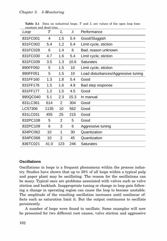
Chapter 3. λ-Monitoring
Table 3.1 Data on industrial loops. T and L are values of the open loop timeconstant and dead time.
Loop T L λ Performance
831FC001 4 1.5 5.4 Good/Sluggish
831FC002 5.4 1.2 5.4 Limit cycle, stiction
831FC028 6 1.4 6 Bad, reason unknown
831FC030 4.7 1.6 5.4 Limit cycle, stiction
831FC039 3.5 1.3 10.6 Saturates
890FF050 5 1.5 10 Limit cycle, stiction
890FF051 5 1.5 10 Load disturbances/Aggressive tuning
831FF160 1.3 1.8 5.4 Good
831FF176 1.5 1.6 4.9 Bad step response
831FF177 1.2 1.5 4.5 Good
890QC040 5.1 2.3 15.3 In manual
831LC361 614 2 304 Good
LC57306 1135 10 562 Good
831LC031 455 25 215 Good
832PC108 5 2 5 Good
832PC109 6 3 6 Aggressive tuning
834PC062 10 1 30 Quantization
834PC068 10 2 45 Quantization
836TC021 41.0 123 246 Saturates
Oscillations
Oscillations in loops is a frequent phenomena within the process indus-try. Studies have shown that up to 30% of all loops within a typical pulpand paper plant may be oscillating. The reason for the oscillations canbe many. Typical ones are problems associated with valves such as valvestiction and backlash. Inappropriate tuning or change in loop gain follow-ing a change in operating region can cause the loop to become unstable.The amplitude of the resulting oscillation increases until nonlinear ef-fects such as saturation limit it. But the output continuous to oscillatepersistently.
A number of loops were found to oscillate. Some examples will nowbe presented for two different root causes, valve stiction and aggressive
102

3.5 Validation on Industrial Data
00.2
0.5
1
0 200 400 600 800 1000 1200 1400 1600
0
1045 1050 10550.2
0.22
0.24
0.26
Minutes
I λe(k)
r(k)
,y(k)
Figure 3.2 Loop 890FF050. Loop with valve stiction. Top graph: Iλ . Middle graph:e(k). Bottom graph: set point r(k) (solid) and output y(k) (dashed).
tuning.
Valve Stiction The most common reason for oscillations was valvestiction. Three flow loops were found to have this problem. In Fig. 3.2the λ-index is shown for one of the loops (loop 890FF050). The indexlies above 0.2 for most of the series length. The lowest graph shows thereference value and the output signals for an interval when Iλ was closeto 0.5. An easily recognizable square-shaped signal form can be noticed.The control signal had the familiar sawtooth shape as well.
Loops 831FC002 and 831FC030 also seemed to have stiction in thevalve. The indices for these loops are shown in Appendix A.
Remark: Dynamic Properties of Recursive Estimator The datafrom the current loops serves well to demonstrate some dynamic proper-ties of the recursive algorithm presented. The original data was sampledwith a sampling time of 1 second. Since λ was equal to 10 seconds, the dataseries was down sampled with a sampling time of 2 seconds. With a data
103
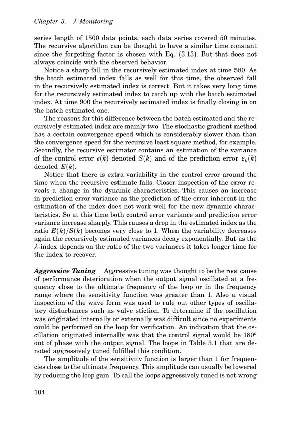
Chapter 3. λ-Monitoring
series length of 1500 data points, each data series covered 50 minutes.The recursive algorithm can be thought to have a similar time constantsince the forgetting factor is chosen with Eq. (3.13). But that does notalways coincide with the observed behavior.
Notice a sharp fall in the recursively estimated index at time 580. Asthe batch estimated index falls as well for this time, the observed fallin the recursively estimated index is correct. But it takes very long timefor the recursively estimated index to catch up with the batch estimatedindex. At time 900 the recursively estimated index is finally closing in onthe batch estimated one.
The reasons for this difference between the batch estimated and the re-cursively estimated index are mainly two. The stochastic gradient methodhas a certain convergence speed which is considerably slower than thanthe convergence speed for the recursive least square method, for example.Secondly, the recursive estimator contains an estimation of the varianceof the control error e(k) denoted S(k) and of the prediction error ε b(k)denoted E(k).
Notice that there is extra variability in the control error around thetime when the recursive estimate falls. Closer inspection of the error re-veals a change in the dynamic characteristics. This causes an increasein prediction error variance as the prediction of the error inherent in theestimation of the index does not work well for the new dynamic charac-teristics. So at this time both control error variance and prediction errorvariance increase sharply. This causes a drop in the estimated index as theratio E(k)/S(k) becomes very close to 1. When the variability decreasesagain the recursively estimated variances decay exponentially. But as theλ-index depends on the ratio of the two variances it takes longer time forthe index to recover.
Aggressive Tuning Aggressive tuning was thought to be the root causeof performance deterioration when the output signal oscillated at a fre-quency close to the ultimate frequency of the loop or in the frequencyrange where the sensitivity function was greater than 1. Also a visualinspection of the wave form was used to rule out other types of oscilla-tory disturbances such as valve stiction. To determine if the oscillationwas originated internally or externally was difficult since no experimentscould be performed on the loop for verification. An indication that the os-cillation originated internally was that the control signal would be 180o
out of phase with the output signal. The loops in Table 3.1 that are de-noted aggressively tuned fulfilled this condition.
The amplitude of the sensitivity function is larger than 1 for frequen-cies close to the ultimate frequency. This amplitude can usually be loweredby reducing the loop gain. To call the loops aggressively tuned is not wrong
104

3.5 Validation on Industrial Data
00.2
0.5
1
0 100 200 300 400 500−0.5
0
0.5
120 121 122 123 124 125
−0.2
0
0.2
Minutes
I λe(k)
e(k),
e(k)
Figure 3.3 Loop 832PC109. Aggressively tuned loop. Top graph: Iλ recursivelyestimated (solid line) and batch wise estimated (∗). Middle graph: e(k). Bottomgraph: e(k) and the predicted error, e(khk− b).
even if the oscillation originates externally since the signal oscillates at afrequency that the sensitivity function amplifies.
In Fig. 3.3 λ-monitoring is applied to the data from a pressure controlloop (Loop 832PC109). In the upper graph, Iλ , is shown calculated batchwise and with the recursive algorithm in Section 3.4. The error is oscil-lating considerably. The period of the oscillation is about 10 sec which isaround 0.6 rad/sec. The ultimate frequency of the loop with the λ-tuningis 0.7 rad/sec.
In the lowest graph of the figure the error e(k) and the b-step aheadpredicted error, e(khk− b) is shown for some minutes. b is equal to (λ +L)/h. It can be seen that the predictor manages to predict parts of theoscillations thus reducing the prediction error. This in turn will cause theIλ to increase.
It is of interest to try to characterize how oscillatory the output sig-nal will have to become before the λ-index indicates poor performance. In
105
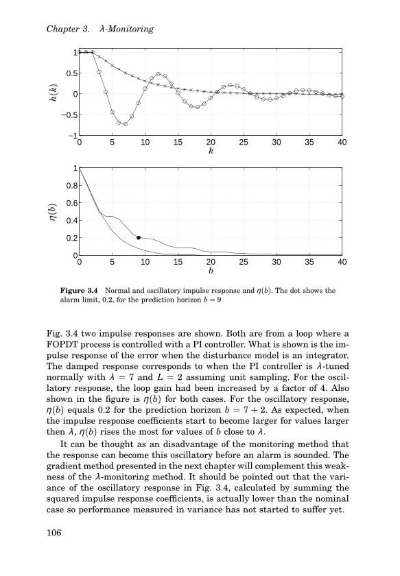
Chapter 3. λ-Monitoring
0 5 10 15 20 25 30 35 40−1
−0.5
0
0.5
1
0 5 10 15 20 25 30 35 400
0.2
0.4
0.6
0.8
1
η(b)
b
k
h(k)
Figure 3.4 Normal and oscillatory impulse response and η(b). The dot shows thealarm limit, 0.2, for the prediction horizon b = 9
Fig. 3.4 two impulse responses are shown. Both are from a loop where aFOPDT process is controlled with a PI controller. What is shown is the im-pulse response of the error when the disturbance model is an integrator.The damped response corresponds to when the PI controller is λ-tunednormally with λ = 7 and L = 2 assuming unit sampling. For the oscil-latory response, the loop gain had been increased by a factor of 4. Alsoshown in the figure is η(b) for both cases. For the oscillatory response,η(b) equals 0.2 for the prediction horizon b = 7 + 2. As expected, whenthe impulse response coefficients start to become larger for values largerthen λ , η(b) rises the most for values of b close to λ .
It can be thought as an disadvantage of the monitoring method thatthe response can become this oscillatory before an alarm is sounded. Thegradient method presented in the next chapter will complement this weak-ness of the λ-monitoring method. It should be pointed out that the vari-ance of the oscillatory response in Fig. 3.4, calculated by summing thesquared impulse response coefficients, is actually lower than the nominalcase so performance measured in variance has not started to suffer yet.
106

3.5 Validation on Industrial Data
A few loops seemed to display the characteristics of aggressive tun-ing, originating inside the loop, for short intervals only. In Appendix Aloops 890FF050 and 890FF051 showed this behavior for very short timeintervals.
Remark In [Kozub, 1997] a monitoring approach was suggested wherethe index to monitor was η(b) but with b equal to the desired settlingtime. It is said that the statistic is valuable when only settling time is ofimportance but that this approach suffers from the fact that large initialtransients in the impulse response go unnoticed. In [Kozub, 1997] thedefinition of the settling time is not given but for a λ-tuned loop thesettling time is usually considered to be equal to 4λ . In the current casethis would mean b = 28. The problem with this approach is then seenin Fig. 3.4. When performance deteriorates η(b) changes first for smallb’s. Before a noticeable change occurs for larger b the performance hasdeteriorated severely.
Sluggish Tuning and Slow Disturbances
If a loop works at many operating regions it is frequent that the tuningends up being the most conservative one or the most robust one over alloperating regions. The reason for this is that as performance problemsoccur at any operating region it is common to detune the controller, typi-cally by lowering the gain, K , in the PI controller. Because of lack of timeof operators the old parameter values are not put back in the controllerwhen the loop operates at the more normal operating region again.
The consequence of this is that many controllers are detuned. Whenload disturbances or set-point changes occur the error signal tends tostay away from zero for a long time. In [Hägglund, 1999] a method todetect sluggish control loops is presented. Both controller output and plantoutput are used to determine if the loop is sluggish. The index describesthe relation between times of positive and negative correlation betweenthe control and plant output increments.
If the error signal stays away from zero for a long period of time, theλ-index will give an alarm indicating bad performance, as it will quicklybe able to predict the error. A sluggish control loop will therefore be dis-covered by the λ monitoring method. On the other hand, if a slow loaddisturbance affects the loop, for example a step or a ramp on the plant in-put, the error signal will also stay away from zero for long periods of time.This will cause the λ-index to indicate poor performance even though theloop might be working well. So it might be claimed that the λ-monitoringmethod will give false alarms when slow disturbances affect the loop. Itmight also be claimed that these alarms will not be false alarms sincethey indicate that the disturbance model used in the design, i.e. a step
107

Chapter 3. λ-Monitoring
disturbance, is incorrect. The problem is that load disturbances might bequite frequent and the operators might not be interested in these alarms.
A remedy would be to redesign the prediction horizon for a differentdisturbance model. It is for these situations that the prediction horizonand alarm level of the λ-index should be considered an engineering cri-terion. On the other hand there is no clear upper limit that should beput on the prediction horizon. If the prediction horizon is designed forload disturbance it will give alarm when a temporary ramp is applied tothe plant input in stead of a step. Furthermore, longer prediction horizonmeans less sensitivity to other faults like aggressive tuning.
The final suggestion is that the prediction horizon should be treatedas an engineering criterion and adjusted if slow disturbances affect theloop. If the slow disturbances are less frequent, an other option wouldbe to expect occasional alarms. When the alarms occur they could triggerinspection or application of the method presented in [Hägglund, 1999] todetermine if tuning is sluggish.
Once again the gradient method will complete the weakness of theλ-monitoring method since it will give information about the frequencycontent of the disturbances.
In Fig. 3.5 data from loop 831FC001 is shown. The batch wise es-timated λ-index is constantly far above 0.2, actually close to 0.7 for thewhole period. The recursively estimated λ-index is always below the batchwise estimated one but does rise quickly above 0.2 so that an alarm issounded. In the bottom graph of Fig. 3.5 the error is shown for a shorterinterval so that the dynamics can be inspected more carefully. It is seenthat the error sometimes stays minutes away from 0, not consistent withthe λ-tuning which is 10 sec. The reason for the sluggishness was a com-bination of bad tuning, the controller gain had been decreased but alsothat the reference value was changing in a ramp like manner.
In Fig. 3.6 the impulse response and η(b) are shown for two systems.Both of them are λ-tuned loops with a integrator as the disturbance model.The faster response has λ = 7 and L = 2. The slower response hasλ = 13. It can be seen that η(b) for the slower response intersects 0.2for prediction horizon b = 9. The conclusion is that if this loop wouldhave been monitored assuming λ = 7 and L = 2, and later detuned, themonitoring would indicate poor performance when the loop would have atime constant of λ = 13. So in this case λ can be almost doubled beforethe λ-index sounds an alarm.
Remark: Stochastic and Deterministic Disturbances Notice thatwith the current formulation no difference is made between stochasticand deterministic disturbances. In both cases the problem can be inter-preted as finding the best b-step ahead predictor and the corresponding
108

3.5 Validation on Industrial Data
00.2
0.5
1
0 100 200 300 400 500−0.1
0
0.1
50 60 70 80 90 100−0.05
0
0.05
Minutes
I λe(k)
e(k),
e(k)
Figure 3.5 Loop 831FC001. Sluggish loop. Top graph: Iλ recursively estimated(solid line) and batch wise estimated (∗). Middle graph: e(k). Bottom graph: e(k)and the predicted error, e(khk− b).
prediction error variance which is compared to the variance of the errorsignal e(k). It is considered a strength that all types of disturbances aretreated in the same way.
In Fig. 3.7 a step change in the set point is shown for the loop 831FF176.This loop was tuned with λ = 4.9 and L = 1.6. As can be seen in the figurethe step response does not fulfill the specifications from the tuning phase.According to the tuning the settling time should be no more than 30 sec.The settling time of the step response in the figure is around 50 sec. Therecursively estimated performance index rises above 0.2 as it should. Another example of a set-point response which does not fulfill design speci-fications is shown in Fig. A.3 in Appendix A. An example of a loop shownin the Appendix that did fulfill design specifications in terms of set-pointresponse was loop 831FF177.
109

Chapter 3. λ-Monitoring
0 5 10 15 20 25 30−0.5
0
0.5
1
0 5 10 15 20 25 300
0.2
0.4
0.6
0.8
1
h(k)
k
η(b)
b
Figure 3.6 Top graph, normal λ-tuned impulse response (x) and sluggish impulseresponse (o). Lower graph, η(b) for normal and sluggish impulse response.
3.6 Conclusions
A nonintrusive performance monitoring method for λ-tuned loops hasbeen described. λ-tuned loops are those loops with an one-degree-of free-dom controller whose set-point response is of first-order plus dead time.λ is the time constant of the set-point response.
The method is thought to be a first indicator of bad performance afterwhich existing diagnosis algorithms could be applied. For online imple-mentation in distributed control systems, a simple recursive algorithm toestimate the index has been presented. All parameters of the monitoringmethod are set by using the tuning. The need for historical informationshould be none or little.
The method applies equally to stochastic or deterministic disturbances.Bad performance is related to low variance of prediction error when thecontrol error is predicted over a time horizon related to the tuning. Lowprediction error variance means high predictability which in turn meansthat the controller has not done a good job rejecting the disturbances
110

3.6 Conclusions
0 50 100 150 200
0
0.2
0.5
1
0 50 100 150 200
0.2
0.3
Seconds
I λr(
k),y(k)
Figure 3.7 Loop 831FF176. Set-point response. Top graph: λ-index recursivelyestimated. Bottom graph: set point r(k) (solid) and output y(k) (dashed). A stepdown occurs in the set point at time 30 sec.
within a suitable time horizon.The method has been tested on 19 λ-tuned PI loops from a Swedish
pulp and paper mill. The method indicated poor performance in manyof the loops. In most of the problem loops a typical root cause could beestablished explaining the poor performance. The method has thereforebeen tested on typical problem loops from the process industry.
111

4
Gradient Monitoring
4.1 Introduction
One of the more frequent acts of maintenance of PID controllers is to ad-just the controller gain. This is often done without a systematic approach,often following the preferences (or whims) of a particular operator. Thereason for the parameter adjustment is usually abnormal variability thatthe operator thinks can be fixed by an adjustment. Abnormal disturbancescan for example occur when the loop is working in a new operating region.
What is shown in this chapter is how to estimate in a simple way agradient of a quadratic cost function with respect to a controller parame-ter. The purpose is to make this already existing maintenance approach,more systematic. By using the gradient, decisions to adjust controller pa-rameters can be made with more information. The plant staff should befamiliar with the controller parameter for which the gradient is calcu-lated. It should also be strongly correlated with plant variability.
It will be shown that in many cases the equations for the gradientbecome particularly simple allowing recursive implementation in mostDCSs. The focus will be on λ-tuned loops but as long as the controller isavailable and a model exists of the closed-loop system, an estimate of thegradient will be possible.
For λ-tuned loops the parameter for which the gradient is calculatedis λ . The reason for this is to keep consistency with the previous chapterand because λ has a nice interpretation as the closed-loop time constant.For loops controlled with a PID an other choice of controller parametermight be the gain K .
The gradient will be interpreted in a simple way from the sensitivityfunction. Furthermore, in the λ-tuning case a normalization of the gra-dient will be presented so that it becomes independent on variance and
112
4.2 Iterative Feedback Tuning
parameter value.The synthetic gradient will be introduced through the IFT (Itera-
tive Feedback Control) framework. It should be noted that similar gra-dient calculations are frequent within the adaptive control community,see [Åström and Wittenmark, 1995] and as within the IFT framework thegradients are used to update the controller parameters to lower the costfunction.
It is possible to use the gradient presented here to initiate adjustmentof the controller parameters to lower the cost function. But no automaticadjustment is considered. An operator is always thought to be “in theloop” of parameter adjustment. The gradient gives information about thespectral content of the disturbances affecting the loop. This informationis compressed into one number related to a controller parameter. As thisinformation can be collected and monitored over time it might provide avaluable overview over the state of the loop and the disturbances affectingit. For example if the gradient is watched over many operating regions itmight indicate opportunities for gain scheduling.
4.2 Iterative Feedback Tuning
Iterative feedback tuning has recently emerged as a technology to tunefixed order controllers like the PID by performing experiments on theclosed-loop system. The tuning is performed by calculating the controllerparameter gradient of a quadratic cost function and modifying the param-eters in the descent direction of this cost function. A reference coveringmost aspects of IFT is [Hjalmarsson et al., 1998].
The method deals with SISO linear systems on the form
y(k) = P(q−1)u(k) +w(k) (4.1)
w(k) is the process disturbance. The controller is assumed to be of onedegree of freedom.
u(k) = C(ρ)(r(k) − y(k)) (4.2)The dependence of transfer functions on the back shift operator q−1 will beomitted in what follows. Instead the dependence on controller parametersρ will be written. The closed-loop system is then given by
y(k) = C(ρ)P1+ C(ρ)P r(k) + 1
1+ C(ρ)Pw(k)= T(ρ)r(k) + S(ρ)w(k) (4.3)
113

Chapter 4. Gradient Monitoring
T(ρ) is the complementary sensitivity function while S(ρ) is the sensi-tivity function. It is easy to check that T + S = 1. The time argument ofthe signals will now be omitted as well but again they will be written asa function of controller parameters ρ.
Let yd be the desired response to the reference signal r. Given thatthe design method resulted in a closed loop transfer function Td thenyd = Tdr. In the case of λ-tuning Td is the first order response with λ asthe time constant. Putting y = y− yd the cost function that is monitoredis of quadratic type,
J(ρ) = 1N
E
[N∑
t=1
y(ρ)2]
(4.4)
For large N, J is an estimate of the variance of y. Notice that y is notequal to the error e(k) in the previous chapter. In the IFT framework aterm containing the square of the input signal can be included. To simplifythe derivation this term is excluded here. The expectation is with respectto the weakly stationary disturbance w.
The question that arises is how VJ/Vρ is obtained. It was shown in[Hjalmarsson et al., 1994] that an estimate of this gradient could be com-puted from signals obtained from closed-loop experiments. Assume thatN measurements of r and y(ρ) have been logged. Measurements fromthis series are denoted with a subscript 1. Elementary calculus gives
VJVρ
= 2N
E
[N∑
t=1
y(ρ)V y(ρ)Vρ
](4.5)
It is assumed thatV y(ρ)Vρ
= V y(ρ)Vρ
From Eq. (4.3) one can see that (dropping the argument of ρ)
V yVρ
=(
P1+ PC
VCVρ
− P2C(1+ PC)2
VCVρ
)r
− P(1+ CP)2
VCVρ
w
= 1CVCVρ
T r − 1CVCVρ
(T2 r + TS w
)Assuming the data is from data series 1, notice now that
T2 r1 + TS w1 = T y1
114

4.3 Monitoring the Gradient
Using this in Eq. (4.6) results in the following equation for V y(ρ)/Vρ
V yVρ
= 1CVCVρ
T (r1 − y1) (4.6)
The above equation implies that it is possible to calculate V y/Vρ by fil-tering r1 − y1 through the complimentary sensitivity function. One wayto obtain this term is to apply r1− y1 as a reference value to the real pro-cess and sampling the output yielding measurement series 2. This givesan estimate with an error S w2 since noise would be added. This is theapproach within the IFT methodology. An other approach is to estimateT with system identification techniques, and filtering r1 − y1 with thisidentified transfer function. This is the approach taken in [Bruyne andCarrette, 1997]. A third approach, and the one used in this paper, is touse T = Td obtained from a design method. The gradient calculated byusing the last two approaches is referred to as synthetic.
In the synthetic gradient case, an estimate of VJVρ is formed by using
one measurement series and evaluating Eq. (4.5). A perfect realization ofy is y1 − Tdr1. Eq. (4.5) can now be written as
VJVρ
= 2N
N∑k=1
(y(k) − Tdr(k)) 1CVCVρ
Td (r(k) − y(k)) (4.7)
The subscript 1 is omitted since all signals come from the same dataseries.
4.3 Monitoring the Gradient
It is suggested that Eq. (4.7) is used to calculate the gradient with respectto the desired control parameter. A recursive algorithm will be presentedin a later section. The number of data points to form the estimate is be-tween 1000-1500 as in the previous chapter on the λ-index. Td is obtainedfrom the design specification. In the case of a λ-tuned loop the controllerparameter of choice is λ with the corresponding set point response. Thefilter 1
CVCVρ will now be presented for a few controllers.
In what follows it will be assumed that λ and L are multiples of thesampling time h. If this is not the case, the closest integer usually is agood enough approximation.
115

Chapter 4. Gradient Monitoring
The Gradient for Common Controllers
The equation for the synthetic gradient is now further evaluated for com-mon controllers. The main transfer function to evaluate is the filter
1CVCVρ(q−1) (4.8)
λ-Tuned PI Controllers The λ-tuning rule for PI-controllers was in-troduced in Section 3.2. In discrete time form, with the integral approxi-mated with a forward approximation, the λ-tuned PI controller becomes
C(q−1) = TKp(L + λ)
(1+ hq−1
T(1− q−1))
This assumes that the parameters of a FOPDT model of the plant areavailable, see Eq. (3.3). Then the filter in Eq. (4.8) becomes
1CVCVλ(q−1) = −1
L + λ(4.9)
In the case of integrating processes, λ enters the controller in a morecomplex way. The controller is
C(q−1) = 2λ + LKp(L + λ)2
(1+ hq−1
(2λ + L)(1− q−1
)
which yields
1CVCVλ(q−1) = −2
L + λλ − (λ − h)q−1
2λ + L + (2λ + L − h)q−1 (4.10)
This is a first-order filter and very simple to implement.
The Dahlin Controller With the expression of the Dahlin controllergiven by Eq. (3.8) the filter becomes
1CVCVλ(q−1) = − 1− q−1
1− aq−1 − (1− a)q−d
ha(1− a)λ2 (4.11)
where a = exp(−h/λ).
116
4.4 Interpretation
General PID A general form for a discrete PID controller on serialform, (see [Åström and Hägglund, 1995]) can be written as
u(k) = K (1+ I(k) + D(k)) (4.12)
where I(k) and D(k) are the derivative and integrating terms. The pa-rameter for which the gradient could be calculated is the gain K . Theequation for the gradient becomes particularly simple in this case as
1CVCVK
(q−1) = 1K
(4.13)
Both equations (4.9) and (4.13) are constants which simplifies the evalu-ation of Eq. (4.7).
In Eq. (4.11) the filter has derivative action. The filter in Eq.(4.10) isclose to have derivative action as well when λ is much larger than h. Butnotice that the signal to which 1
CVCVρ is applied in Eq. (4.7) is first filtered
with Td which always has low-pass character.
4.4 Interpretation
Insight into what information the gradient gives can be obtained fromParseval’s relation which relates the cost function in Eq. (4.4) with afrequency domain expression
J(ρ) � 12π
∫ π
−πhS(ρ)h2Φww (4.14)
where S is the sensitivity function. Here it is assumed that the referencevalue is constant and the error is explained solely by the disturbancew(k). Φww is the spectra of the disturbance. The controller parameters af-fect the sensitivity function by lifting up or dragging down the amplitudeon specific frequency intervals. If the power spectrum of the disturbancesis concentrated in a frequency region where an increase in a parame-ter increases the amplitude of the sensitivity function, the gradient withregard to this parameter will be positive. If the sensitivity function am-plitude is reduced with a positive change in the parameter the gradientwill be negative.
The sensitivity function is shown in Fig. 4.1 for a λ-tuned loop. As seenin the figure, a decrease in λ pulls down the low frequency gain while thegain above approximately 1/λ will be larger than 1. Above 1/λ , a decreasein λ pushes the amplitude up. If the disturbances would be concentratedin this frequency region the gradient would be negative.
117

Chapter 4. Gradient Monitoring
10−2
10−1
100
100
λ=7λ=5λ=9
Figure 4.1 Sensitivity function for a λ-tuned loop with L = 2 and varying λ .
Normalized Gradient
The number returned from the gradient estimation in Eq. (4.7) dependson the process and also on the variance of the loop. It is of interest toobtain a more absolute number which does not depend on the processcharacteristics as such but rather, when calculated for a new process,similar numerical values should mean the same thing. One way to dothis is to normalize the gradient obtained with Eq. (4.7). Denoting thenormalized gradient as β , a straight forward way of doing this in the caseof λ-tuned controllers is
β = VJVλ
λJ
(4.15)
As a dimensionless number it is informative to know what numericalvalues this number attains and what they mean. To investigate this anassumption has to be made about the disturbances affecting the system.Assume now that the disturbance is concentrated at one dominating fre-quency. Approximately the disturbance can then be represented with onesinusoidal of frequency ω 0. As a sampled system is considered it is as-
118
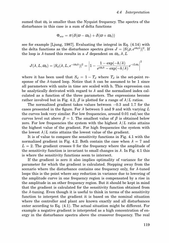
4.4 Interpretation
sumed that ω 0 is smaller than the Nyquist frequency. The spectra of thedisturbance in this case is a sum of delta functions
Φww = π (δ (ω −ω 0) + δ (ω +ω 0))
see for example [Ljung, 1987]. Evaluating the integral in Eq. (4.14) withthe delta functions as the disturbance spectra gives J = hS(ρ, eiω 0h)h2. Ifthe loop is λ-tuned this results in a J dependent on ω 0, λ, L
J(λ, L,ω 0) = hSd(λ, L, e−iω 0h)h2 =∣∣∣∣1− 1− exp(−h/λ)
eiω 0h − exp(−h/λ) e−iLω 0
∣∣∣∣2where it has been used that Sd = 1 − Td where Td is the set-point re-sponse of the λ-tuned loop. Notice that h can be assumed to be 1 sinceall parameters with units in time are scaled with h. This expression canbe analytically derivated with regard to λ and the normalized index cal-culated as a function of the three parameters. The expressions becomerather involved but in Fig. 4.2, β is plotted for a range of λ/L ratios.
The normalized gradient takes values between −0.3 and 1.7 for thecases presented in the figure. For λ between 5 and 9 and with varying Lthe curves look very similar. For low frequencies, around 0.01 rad/sec thecurves level out above β = 1. The smallest value of β is obtained belowzero. For low frequencies the system with the highest λ/L ratio attainsthe highest value of the gradient. For high frequencies the system withthe lowest λ/L ratio attains the lowest value of the gradient.
It is of value to compare the sensitivity functions in Fig. 4.1 with thenormalized gradient in Fig. 4.2. Both contain the case when λ = 7 andL = 2. The gradient crosses 0 for the frequency where the amplitude ofthe sensitivity function is invariant to small changes in λ . In Fig. 4.1 thisis where the sensitivity functions seem to intersect.
If the gradient is zero it also implies optimality of variance for theparameter for which the gradient is calculated. Stepping away from thescenario where the disturbance contains one frequency only, for λ-tunedloops this is the point where any reduction in variance due to lowering ofthe amplitude curve in one frequency region is compensated by a rise inthe amplitude in an other frequency region. But it should be kept in mindthat the gradient is calculated for the sensitivity function obtained fromthe λ-tuning. Even though it is useful to think in terms of the sensitivityfunction to interpret the gradient it is based on the nominal situationwhere the controller and plant are known exactly and all disturbancesenter according to Eq. (4.1). The actual situation might be different. Forexample a negative gradient is interpreted as a high concentration of en-ergy in the disturbance spectra above the crossover frequency. The real
119

Chapter 4. Gradient Monitoring
10−2
10−1
100
−0.5
0
0.5
1
1.5
2β
ω
Figure 4.2 Normalized gradient β for λ = 7 and L = 1, 2, 3. For low frequenciesthe lowest curve has the largest L.
reason is not unlikely aggressive tuning of the loop. Aggressive tuningwith a slight model-plant mismatch will result in a real sensitivity func-tion that has a very large amplitude peak above but close to the crossoverfrequency. This high peak will amplify frequencies in the disturbance spec-tra which will become dominant in the output.
The normalized gradient should be thought of as a coarse spectral anal-ysis where the disturbance spectra is compared to the sensitivity functionfrom the controller design stage and the result squeezed into one num-ber related to the most important tuning parameter. Considering againthe two figures, Figs. 4.1 and 4.2 a positive gradient close to or above 1means that most of the disturbances are of low frequency character. Forsuch a loop there might be opportunities to increase the gain of the con-troller and make it more aggressive without amplifying too much highfrequency noise. A negative gradient means variability should decreaseif the controller is made less aggressive. To give a point of reference forwhat would be a “normal” gradient, for a λ-tuned loop with a disturbance
120

4.5 Recursive Implementation of the Normalized Gradient
model which is an integrator the gradient lies around 0.5− 0.7.
4.5 Recursive Implementation of the Normalized Gradient
A recursive implementation will now be presented for the case of λ-tunedPI controllers. The difference between this case and other cases lies inthe filter 1
CVCVρ and perhaps the specified set-point response Td. To create
the recursive version of the gradient, it is the sum in Eq. (4.7) which isexpressed on recursive form with a forgetting of older values. It is assumedthat the available signals are {y(k), r(k)}.
Some of the signals need to be filtered with the set-point responseobtained from the λ tuning. A discrete form of this transfer function is
Td(q) = 1− exp(−h/λ)1− exp(−h/λ)q−1 q−d
see Section 3.2 where the λ-tuning is introduced. A filtered signal, e(k) isdenoted ef (k). The recursive form is
y(k) = (y(k) − r f (k))γ (k) = −2
λ + Ly(k)(r f (k) − yf (k))
G(k) = lG(k− 1) + γ (k)S(k) = lS(k− 1) + ε 2(k)β (k) = G(k)/S(k)λ
G(k) denotes the gradient sum in Eq. (4.7). S(k) is the variance sum.Notice it is not the same as the one that was calculated in the recursiveequations for the λ-monitoring algorithm. l is the forgetting factor. If theset point is not changing, ε (k) is the controller error, e(k). If the set pointis changing, ε (k) is the error between y(k) and r(k) taking the responseof the closed-loop system into account.
4.6 Use of the Gradient
In this section some of the possible uses of the gradient will be demon-strated. To begin with, a motivating example based on simulations will bepresented. Then two applications of the gradient on industrial data will beconsidered. One will deal with detecting aggressive tuning of loops. Theother addresses detection of sluggish loops. The gradient is shown for theloops presented in Appendix A. Other possible uses of the gradient willbe discussed in the section on future work.
121
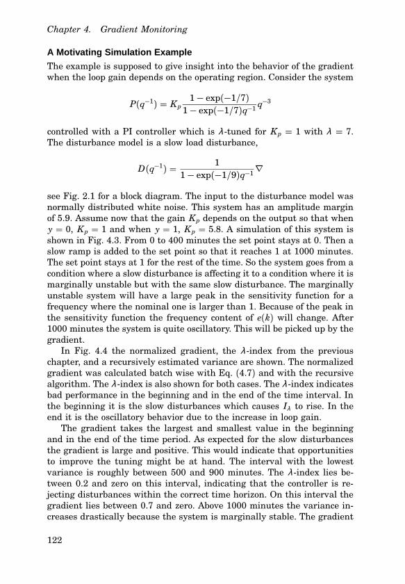
Chapter 4. Gradient Monitoring
A Motivating Simulation Example
The example is supposed to give insight into the behavior of the gradientwhen the loop gain depends on the operating region. Consider the system
P(q−1) = Kp1− exp(−1/7)
1− exp(−1/7)q−1 q−3
controlled with a PI controller which is λ-tuned for Kp = 1 with λ = 7.The disturbance model is a slow load disturbance,
D(q−1) = 11− exp(−1/9)q−1∇
see Fig. 2.1 for a block diagram. The input to the disturbance model wasnormally distributed white noise. This system has an amplitude marginof 5.9. Assume now that the gain Kp depends on the output so that wheny = 0, Kp = 1 and when y = 1, Kp = 5.8. A simulation of this system isshown in Fig. 4.3. From 0 to 400 minutes the set point stays at 0. Then aslow ramp is added to the set point so that it reaches 1 at 1000 minutes.The set point stays at 1 for the rest of the time. So the system goes from acondition where a slow disturbance is affecting it to a condition where it ismarginally unstable but with the same slow disturbance. The marginallyunstable system will have a large peak in the sensitivity function for afrequency where the nominal one is larger than 1. Because of the peak inthe sensitivity function the frequency content of e(k) will change. After1000 minutes the system is quite oscillatory. This will be picked up by thegradient.
In Fig. 4.4 the normalized gradient, the λ-index from the previouschapter, and a recursively estimated variance are shown. The normalizedgradient was calculated batch wise with Eq. (4.7) and with the recursivealgorithm. The λ-index is also shown for both cases. The λ-index indicatesbad performance in the beginning and in the end of the time interval. Inthe beginning it is the slow disturbances which causes Iλ to rise. In theend it is the oscillatory behavior due to the increase in loop gain.
The gradient takes the largest and smallest value in the beginningand in the end of the time period. As expected for the slow disturbancesthe gradient is large and positive. This would indicate that opportunitiesto improve the tuning might be at hand. The interval with the lowestvariance is roughly between 500 and 900 minutes. The λ-index lies be-tween 0.2 and zero on this interval, indicating that the controller is re-jecting disturbances within the correct time horizon. On this interval thegradient lies between 0.7 and zero. Above 1000 minutes the variance in-creases drastically because the system is marginally stable. The gradient
122

4.6 Use of the Gradient
−0.5
0
0.5
1
1.5
0 200 400 600 800 1000 1200−0.1
−0.05
0
0.05
0.1
Minutes
y(k)
e(k)
Figure 4.3 Simulation example. Bottom graph: control error e(k). Top graph: plantoutput y(k).
is negative on this interval indicating that variance could be reduced byincreasing λ .
This example shows that valuable information can be obtained by mon-itoring the gradient. With regard to the previous mentioned praxis of pa-rameter adjustment, the gradient would indicate the following parameteradjustment opportunities. In the beginning of the time interval, the wayto reduce variability would be to decrease λ . Since the gradient is largeand positive, the loop is mostly affected by low frequency disturbances. Adecrease in λ would most probably reduce the effect of these disturbanceswithout increasing the amplitude of the high frequency disturbances toomuch. In the end of the time interval the disturbances affecting the loophave most of their energy concentrated in the region where the sensitiv-ity function amplifies the disturbances. λ should be increased to make thetuning less aggressive.
As mentioned before, it is common that the tuning of a loop ends upbeing the most conservative over all operating regions. In the currentexample, if the loop is expected to work at y = 1 the tuning of the loop
123
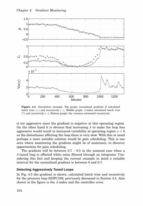
Chapter 4. Gradient Monitoring
−0.5
0
0.5
1
1.5
00.2
0.5
1
0 200 400 600 800 1000 12000
2
4
x 10−4
Minutes
βV
ar(e)
I λ
Figure 4.4 Simulation example. Top graph: normalized gradient β calculatedbatch wise (+) and recursively (−). Middle graph: λ-index calculated batch wise(*) and recursively (−). Bottom graph: the variance estimated recursively.
is too aggressive since the gradient is negative at this operating region.On the other hand it is obvious that increasing λ to make the loop lessaggressive would result in increased variability at operating region y = 0as the disturbance affecting the loop there is very slow. With this in mindperhaps a more suitable solution would be gain scheduling. This is onearea where monitoring the gradient might be of assistance, to discoveropportunities for gain scheduling.
The gradient will be between 0.7 − 0.5 in the nominal case when aλ-tuned loop is affected white noise filtered through an integrator. Con-sidering this fact and keeping the current example in mind a suitableinterval for the normalized gradient is between 0 and 0.7.
Detecting Aggressively Tuned Loops
In Fig. 4.5 the gradient is shown, calculated batch wise and recursivelyfor the pressure loop 823PC109, previously discussed in Section 3.5. Alsoshown in the figure is the λ-index and the controller error.
124

4.6 Use of the Gradient
−0.5
0
0.5
1
00.2
0.5
1
0 100 200 300 400 500−0.5
0
0.5
Minutes
I λe(k)
β
Figure 4.5 Loop 823PC109. Top graph: β estimated batch wise and recursively.Middle graph: λ-index. Bottom graph: e(k).
The gradient is close to zero or negative over the whole interval. Aloop with negative gradient presents a very clear opportunity to reducevariability in the plant by adjusting the relevant parameter. In this casethe λ could have been increased. The fact that the λ-index is well above 0.2for most of the interval also indicates that the loop has problems. Neitherthe λ-index nor the gradient indicates that the oscillation observed is dueto aggressive tuning of the loop. But in either case an adjustment of thecontroller parameters is justified since even if the disturbances originateoutside the loop, their spectral composition is such that the current loop isincreasing the variability instead of decreasing it. The appropriate actionis still to increase λ .
Detecting Sluggish Loops
In Fig. 4.6 the normalized gradient is shown for the flow loop 831FC001,previously discussed in Section 3.5.
It takes some time for the recursively estimated gradient to settle atthe same level as the gradient estimated batch wise. But it settles at a
125
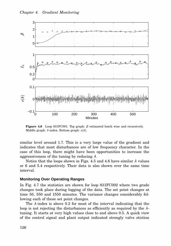
Chapter 4. Gradient Monitoring
0
1
2
3
00.2
0.5
1
0 100 200 300 400 500−0.1
0
0.1
Minutes
I λe(k)
β
Figure 4.6 Loop 831FC001. Top graph: β estimated batch wise and recursively.Middle graph: λ-index. Bottom graph: e(k).
similar level around 1.7. This is a very large value of the gradient andindicates that most disturbances are of low frequency character. In thecase of this loop, there might have been opportunities to increase theaggressiveness of the tuning by reducing λ .
Notice that the loops shown in Figs. 4.5 and 4.6 have similar λ valuesor 6 and 5.4 respectively. Their data is also shown over the same timeinterval.
Monitoring Over Operating Ranges
In Fig. 4.7 the statistics are shown for loop 831FC002 where two gradechanges took place during logging of the data. The set point changes attime 50, 550 and 1550 minutes. The variance changes considerably fol-lowing each of these set point changes.
The λ-index is above 0.2 for most of the interval indicating that theloop is not rejecting the disturbances as efficiently as required by the λ-tuning. It starts at very high values close to and above 0.5. A quick viewof the control signal and plant output indicated strongly valve stiction
126
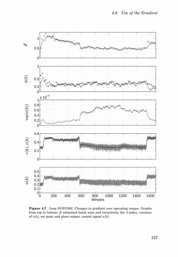
4.6 Use of the Gradient
0
0.5
1
00.2
0.5
1
00.20.40.60.8
1x 10
−3
0
0.2
0.4
0.6
0 200 400 600 800 1000 1200 1400 16000
0.10.20.30.40.5
Minutes
η(b)
u(k)
βr(
k),y(k)
var(
e(k))
Figure 4.7 Loop 831FC002. Changes in gradient over operating ranges. Graphsfrom top to bottom: β estimated batch wise and recursively, the λ-index, varianceof e(k), set point and plant output, control signal u(k).
127
Chapter 4. Gradient Monitoring
as the root cause of the problem. This is shown in greater detail in Fig.A.6. The assumption of linearity previously discussed does therefore nothold for this loop. This fact might explain other unexpected observationswithin the data series.
The set point is changed at time 50 from 0.25 to 0.5 approximately.Following the change there is a notable drop in variance. The gradientsettles around 1 indicating slow disturbances at the new set-point level.The slow disturbances seem to be caused by the stiction but the frequencyof the limit cycle is considerably reduced from the time interval 0 − 50.This indicates lower integral gain. As the integral gain was not changedspecially in the PI controller over the time the lower integral gain canonly be explained by a lower process gain for the new operating region.Then from time 50 to 550 minutes the gradient is decreasing as varianceis increasing. The stiction pattern is still apparent but more difficult todistinguish as the set point is changed as well. The decreasing gradientimplies that the spectral composition of the control error is moving up tohigher frequencies. This in turn indicates increasing loop gain over theinterval. Notice that in a flow loop with a valve actuator the gain caneasily change when pressure difference over the valve changes. Then attime 550 the set point is changed back to 0.3, close to the previous levelof 0.25. This is followed by a very big increase in variance and significantdrop in the gradient down to 0.5. Again one can suspect that the reasonfor increased variance is an increase in loop gain.
Some conclusions from these observations will now be summarized.The change in loop gain at the different operating regions is picked up bythe gradient as there is a change in the spectral composition of the error.However, the linearity assumption which is important for any spectralanalysis, does not hold for this loop. As can be expected there are in-consistencies in the information obtained from the gradient. The largestvalue of the gradient is in the beginning of the interval 50 to 550 minutes.There it is above 1 indicating a sluggish loop. But this is the point wherethe loop has lowest variability. The gradient has a value of 0.5 at the op-erating level with the largest variance, between 550 and 1550 minutes.The numerical value of 0.5 for the gradient should be acceptable. But thefact that the λ-index is above 0.2 for the whole interval should indicatethat something is wrong with the loop. A conclusion is that if there are“strong” nonlinearities in the loop the information from the gradient willnot be reliable.
128
4.7 Discussions and Future Work
4.7 Discussions and Future Work
Missing in the treatment are results from experiments in an industrialenvironment where gradient data has been used in a more proactive wayto reduce variability and optimize performance. If it is of interest to keepcertain loops tightly tuned, λ could be trimmed until the gradient wouldbe on the interval 0− 0.7. As long as variability would drop, the closer tozero the better.
For loops known to have different disturbance characteristics for dif-ferent operating regions the gradient might give information valuable forimplementation of gain scheduling.
For most of the industrial data, when the λ-index indicated good per-formance, i.e. Iλ was below 0.2, the normalized gradient was found to lieon the interval [0, 0.7]. An example of this can be seen in Appendix Afor two of the loops. Consider the loops 831FF176 and 831FF177 whichhave long intervals of good performance. Both loops have intervals wherethe control signal saturates but outside of these intervals Iλ is below 0.2.When Iλ is below 0.2 the gradients are positive and close to zero. Loop890FF051 shows similar behavior if the batch wise estimated statisticsare considered. The gradient is actually above 0.7 but always below 1.
4.8 Conclusions
A statistic has been presented which gives useful information regardingthe assumed sensitivity function and the disturbances affecting the loop.The statistic is an estimate of the partial derivative of the variance, withregard to a control parameter.
It has been shown that the evaluation of this gradient is very simplefor many common controllers. A recursive version has been presented thatshould be implementable in most distributed control systems. In the caseof λ-tuning the gradient has been shown to have a nice interpretationby considering the sensitivity function of the λ-tuned loop. A normaliza-tion of the gradient has been presented as well and it has been shownthat its numerical values should lie between 0 and 0.7. The gradient wascalculated for the industrial data presented in Chapter 3. For most ofthe industrial data, the condition of good performance according to theλ-index was almost always followed by a value of the gradient on thedesirable interval.
The fact that the statistic is related to a simple tuning rule shouldfacilitate its acceptance in an industrial environment.
129

A
Industrial data
Data from some of the loops in Table 3.1 is shown on the following pagesalong with the λ-index, Iλ , and the normalized gradient, β . Most loopsshown here were found to have some kind of performance problem. Somegood loops where the λ-index was below 0.2 most of the time are includedas well.
130
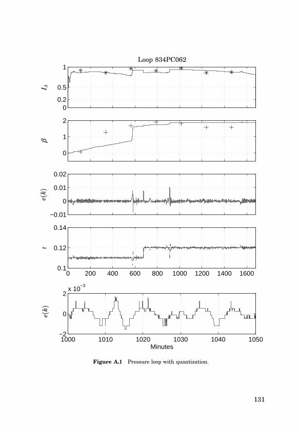
00.2
0.5
1
0
1
2
−0.01
0
0.01
0.02
0 200 400 600 800 1000 1200 1400 16000.1
0.12
0.14
r
1000 1010 1020 1030 1040 1050−2
0
2x 10
−3
Minutes
I λβ
e(k)
e(k)
Loop 834PC062
Figure A.1 Pressure loop with quantization.
131

Appendix A. Industrial data
00.2
0.5
1
0
1
2
−0.1
−0.05
0
0.05
0.1
0 200 400 600 800 1000 1200 1400 16000
0.5
1
1.5
1250 1260 1270 1280 1290 13000.5
0.52
0.54
Minutes
I λβ
e(k)
r(k)
,y(k)
r(k)
,y(k)
Loop 831FC030
Figure A.2 Flow loop with stiction. The lowest graph shows the set point andoutput on an interval where the stiction square wave pattern was apparent.
132
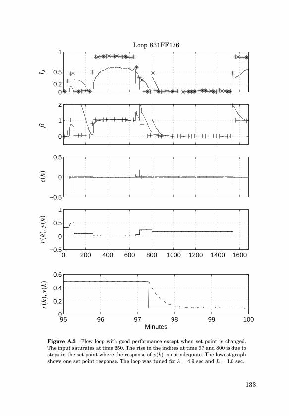
00.2
0.5
1
0
1
2
−0.5
0
0.5
0 200 400 600 800 1000 1200 1400 1600−0.5
0
0.5
1
95 96 97 98 99 1000
0.2
0.4
0.6
Minutes
I λβ
e(k)
r(k)
,y(k)
r(k)
,y(k)
Loop 831FF176
Figure A.3 Flow loop with good performance except when set point is changed.The input saturates at time 250. The rise in the indices at time 97 and 800 is due tosteps in the set point where the response of y(k) is not adequate. The lowest graphshows one set point response. The loop was tuned for λ = 4.9 sec and L = 1.6 sec.
133
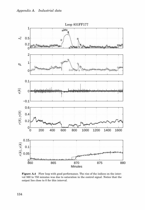
Appendix A. Industrial data
00.2
0.5
1
0
1
2
−0.1
0
0.1
0 200 400 600 800 1000 1200 1400 16000
0.2
0.4
0.6
860 865 870 875 8800
0.05
0.1
0.15
Minutes
I λβ
e(k)
r(k)
,y(k)
r(k)
,y(k)
Loop 831FF177
Figure A.4 Flow loop with good performance. The rise of the indices on the inter-val 560 to 750 minutes was due to saturation in the control signal. Notice that theoutput lies close to 0 for this interval.
134

00.2
0.5
1
0
1
2
3
0
0 200 400 600 800 1000 1200 1400 16000.5
0.6
0.7
0.8
40 45 50 55 60 65 70 75 800.65
0.7
0.75
Minutes
I λβ
e(k)
r(k)
,y(k)
r(k)
,y(k)
Loop 831LC031
Figure A.5 Level control loop. Due to large λ (215 seconds) only two batch esti-mates were calculated. Load disturbance at time 45 minutes causes a rise in Iλ .
135

Appendix A. Industrial data
00.2
0.5
1
0
1
2
0
0 200 400 600 800 1000 1200 1400 16000
0.2
0.4
0.6
30 32 34 36 38 400.2
0.3
0.4
Minutes
I λβ
e(k)
r(k)
,y(k)
r(k)
,y(k)
Loop 831FC002
Figure A.6 Flow loop with stiction. The lowest graph shows the set point andoutput on an interval where the stiction square wave pattern was apparent.
136
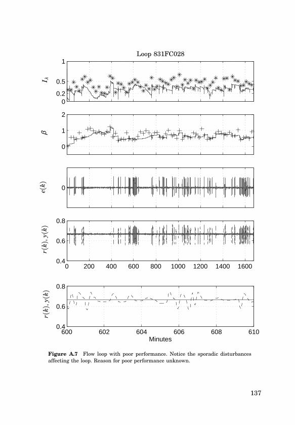
00.2
0.5
1
0
1
2
0
0 200 400 600 800 1000 1200 1400 16000.4
0.6
0.8
600 602 604 606 608 6100.4
0.6
0.8
Minutes
I λβ
e(k)
r(k)
,y(k)
r(k)
,y(k)
Loop 831FC028
Figure A.7 Flow loop with poor performance. Notice the sporadic disturbancesaffecting the loop. Reason for poor performance unknown.
137

Appendix A. Industrial data
00.2
0.5
1
0
1
2
0
0 200 400 600 800 1000 1200 1400 16000
0.5
1
1045 1050 10550.2
0.22
0.24
0.26
Minutes576 578 580
0.4
0.6
0.8
1
Minutes
I λβ
e(k)
r(k)
,y(k)
r(k)
,y(k)
Loop 890FF050
Figure A.8 Flow loop with stiction. The lowest graph to the left shows the set pointand output on an interval where the stiction square wave pattern was apparent.Notice that the gradient dives at time 576. The graph to the right shows an intervalwhere the output y(k) displayed oscillatory behavior with the characteristics ofinstability.
138
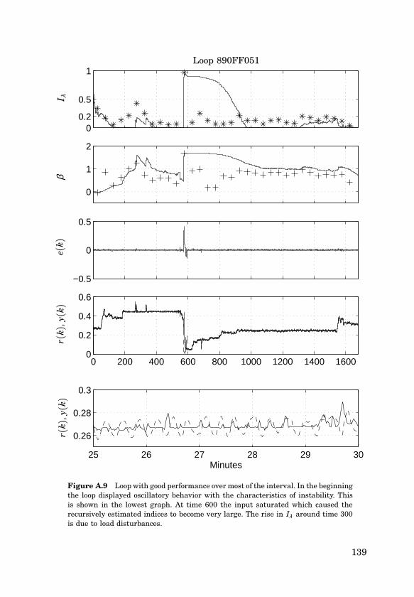
00.2
0.5
1
0
1
2
−0.5
0
0.5
0 200 400 600 800 1000 1200 1400 16000
0.2
0.4
0.6
25 26 27 28 29 30
0.26
0.28
0.3
Minutes
I λβ
e(k)
r(k)
,y(k)
r(k)
,y(k)
Loop 890FF051
Figure A.9 Loop with good performance over most of the interval. In the beginningthe loop displayed oscillatory behavior with the characteristics of instability. Thisis shown in the lowest graph. At time 600 the input saturated which caused therecursively estimated indices to become very large. The rise in Iλ around time 300is due to load disturbances.
139

Bibliography
Åström, K. J. (1967): “Computer control of a paper machine—An applica-tion of linear stochastic control theory.” IBM Journal of Research andDevelopment, 11:4, pp. 389–405.
Åström, K. J. (1970): Introduction to Stochastic Control Theory. AcademicPress, New York.
Åström, K. J. and T. Hägglund (1995): PID Controllers: Theory, Design,and Tuning. Instrument Society of America, Research Triangle Park,North Carolina.
Åström, K. J. and T. Hägglund (2001): “The future of PID control.” ControlEngineering Practice, 9, pp. 1163–1175.
Åström, K. J., C. C. Hang, and B. C. Lim (1994): “A new Smith predictorfor controlling a process with an integrator and long dead-time.” IEEETransactions on Automatic Control, 39:2.
Åström, K. J. and B. Wittenmark (1995): Adaptive Control. Addison-Wesley, Reading, Massachusetts.
Åström, K. J. and B. Wittenmark (1997): Computer-Controlled Systems.Prentice Hall.
Bialkowski, W. (1993): “Dreams versus reality: a view from both sides ofthe gap.” Pulp and Paper Canada.
Bialkowski, W. (1998): “Mill audits can cut costs by reducing control loopvariability.” Pulp & Paper.
Bruyne, F. and P. Carrette (1997): “Synthetic generation of the gradientfor an iterative controller optimization method.” In 4th EuropeanControl Conference.
Dahlin, E. B. (1968): “Designing and tuning digital controllers.” Instru-ments and Control Systems, 42, June, pp. 77–83.
140
Desborough, L. and T. Harris (1992): “Performance assessment measuresfor univariate feedback control.” The Canadian Journal of ChemicalEngineering, 70, pp. 1186–1197.
Desbourough, L. and R. Miller (2001): “Increasing customer value ofindustrial control performance monitoring - honeywell’s experience.”In Sixth International Conference on Chemical Process Control, vol. 98of AIChE Symposium Series.
Devries, W. and S. Wu (1978): “Evaluation of process control effectivenessand diagnosis of variation in paper basis weight via multivariatetime-series analysis.” IEEE Transaction on Automatic Control, 23:4,pp. 702–708.
Doyle, J., B. Francis, and A. Tannenbaum (1992): Feedback ControlTheory. Macmillan Publishing Company: New York.
Ender, D. (1993): “Process control performance: not as good as you think.”Control Engineering, September.
Eriksson, P.-G. and A. Isaksson (1994): “Some aspects of control loop per-formance monitoring.” In 3rd IEEE conference on Control Applications.Glasgow, Scotland.
Gustafsson, F. and S. F. Graebes (1998): “Closed-loop performance moni-toring in the presence of system changes and disturbances.” Automat-ica, 34:11, pp. 1311–1326.
Hägglund, T. (1995): “A control-loop performance monitor.” Control Engi-neering Practice, 3, pp. 1543–1551.
Hägglund, T. (1996): “An industrial dead-time compensating PI con-troller.” Control Engineering Practice, 4, pp. 749–756.
Hägglund, T. (1999): “Automatic detection of sluggish control loops.”Control Engineering Practice, 7, pp. 1505–1511.
Hägglund, T. (2002): “Industrial applications of automatic performancemonitoring tools.” In IFAC World Congress. Barcelona, Spain.
Harris, H. (1989): “Assessment of control loop performance.” The Cana-dian Journal of Chemical Engineering, 67, pp. 856–861.
Harris, T., F. Boudreau, and J. MacGregor (1996): “Performance assess-ment of multivariable feedback controllers.” Automatica, 32, pp. 1503–1517.
Harris, T., C. Seppala, and L. Desborough (1999): “A review of perfor-mance monitoring and assessment techniques for univariate and mul-tivariate control systems.” Journal of Process Control, 9, pp. 1–17.
141

Bibliography
Harris, T., C. Seppala, P. Jofriet, and B. Surgenor (1996): “Plant-widefeedback control performance assessment using and expert-systemframework.” Control Engineering Practice, 4:9, pp. 1297–1303.
Hjalmarsson, H., M. Gevers, S. Gunnarsson, and O. Lequin (1998):“Iterative feedback tuning: Theory and applications.” IEEE ControlSystems, August.
Hjalmarsson, H., S. Gunnarsson, and M. Gevers (1994): “A convergentiterative restricted complexity control design scheme.” In Proc. 33rdIEEE Conference on Decision and Control, pp. 1735–1740. Orlando,Florida.
Horch, A. (2000): Condition Monitoring of Control Loops. PhD thesis,Department of Signals, Sensors and Systems, Royal Institute ofTechnology.
Horch, A. and A. Isaksson (1999): “A modified index for control perfor-mance assessment.” Journal of Process Control, 9, pp. 475–483.
Huang, B. (1999): “Performance assessment of processes with abruptchanges of disturbances.” The Chanadian Journal of Chemical Engi-neering, 77, pp. 1044–1054.
Huang, B. and S. L. Shah (1998): “Practical issues in multivariablefeedback control performance assessment.” Journal of Process Control,8, pp. 421–430.
Huang, B., S. L. Shah, and E. Kwok (1997): “Good, bad or optimal?performance assessment of multivariable processes.” Automatica, 33,pp. 1175–1183.
Ingimundarson, A. and T. Hägglund (2000a): “Closed-loop identificationof first-order plus dead-time model with method of moments.” InADCHEM 2000, IFAC International Symposium on Advanced Controlof Chemical Processes. Pisa, Italy.
Ingimundarson, A. and T. Hägglund (2000b): “Robust automatic tuning ofan industrial PI controller for dead-time systems.” In IFAC Workshopon Digital Control – Past, present, and future of PID Control. Terrassa,Spain.
Ingimundarson, A. and T. Hägglund (2001): “Robust tuning procedures fordead-time compensating controllers.” Control Engineering Practice, 9,pp. 1195–1208.
Isaksson, A. (1996): “PID controller performance assessment.” In Proc.Control Systems, Halifax, NS.
142

Jofriet, P. and W. Bialkowski (1996): “Process knowledge: The key to on-line monitoring of process variability and control loop performance.”In Control Systems ’96. Halifax.
Kendar, S. J. and A. Cinar (1997): “Controller performance assessmentby frequency domain techniques.” Journal of Process Control, 7:3,pp. 181–194.
Ko, B.-S. and T. F. Edgar (1998): “Assessment of achievable PI controlperformance for linear processes with dead time.” In Proc. AmericanControl Conference, Philadelphia, Pennsylvania.
Kozub, D. and C. Garcia (1993): “Monitoring and diagnosis of automatedcontrollers in the chemical process industries.” In Proc. AIChE.St.Louis.
Kozub, D. J. (1997): “Controller performance monitoring and diagnosis:Experiences and challenges.” In AIChE Symposium Series. AIChE.
Kozub, D. J. (2002): “Controller performance monitoring and diagnosis. in-dustrial perspective.” In Proceedings of the 15th IFAC World Congress,Barcelona, Spain.
Landau, I., D. Rey, A. Karimi, A. Voda, and A. Franco (1995): “Aflexible transmission system as a benchmark for robust digital control.”Proceedings of the Third European Control Conference, Rome, Italy.
Laughlin, D., D. Rivera, and M. Morari (1987): “Smith predictor designfor robust performance.” Int. J. Control, 46, pp. 477–504.
Lee, T., Q. Wang, and K. Tan (1995): “Automatic tuning of the Smithpredictor controller.” Journal of Systems Engineering, 5.
Lee, T., Q. Wang, and K. Tan (1996): “Robust Smith-predictor controllerfor uncertain delay systems.” AIChE Journal, 42.
Ljung, L. (1987): System Identification—Theory for the User. PrenticeHall, Englewood Cliffs, New Jersey.
Ljung, L. (1999): System Identification—Theory for the User, SecondEdition. Prentice Hall.
Majhi, S. and D. Atherton (2000): “Obtaining controller parameters fora new Smith predictor using autotuning.” Automatica, 36, pp. 1651–1658.
Marlin, T. (1995): Process Control. Designing Processes and Control Sys-tems for Dynamic Performance. McGraw-Hill International Editions.
143

Bibliography
Matausek, M. and A. Micic (1996): “A modified smith predictor forcontrolling a process with an integrator and long dead-time.” IEEETransaction on Automatic Control, 41, pp. 1199–1203.
Matausek, M. and A. Micic (1999): “On the modified smith predictor forcontrolling a process with an integrator and long dead-time.” IEEETransaction on Automatic Control, 44, pp. 1603–1606.
Meinsma, G. and H. Zwart (2000): “On H∞ control for dead-time systems.”IEEE Transaction on Automatic Control, 45.
Meyer, C., D. E. Seborg, and R. K. Wood (1976): “A comparison ofthe Smith predictor and conventional feedback control.” ChemicalEngineering Science.
Morari, M. and E. Zafiriou (1989): Robust Process Control. Prentice-Hall,Englewood Cliffs, New Jersey.
Normey-Rico, J., C. Bordons, and E. Camacho (1997): “Improving therobustness of dead-time compensating PI controllers.” Control Engi-neering Practice, 5, pp. 801–810.
Normey-Rico, J. and E. Camacho (1999): “Robust tuning of dead-timecompensators for processes with an integrator and long dead-time.”IEEE Transaction on Automatic Control, 44, pp. 1597–1603.
Normey-Rico, J. and E. Camacho (2002): “A unified approach to designdead-time compensators for stable and integrative processes withdead-time.” IEEE Transaction on Automatic Control, 47, pp. 299–305.
Palmor, Z. (1980): “Stability properties of smith dead-time compensatorcontrollers.” Int. J. Control, 32, pp. 937–949.
Palmor, Z. and M. Blau (1994): “An auto-tuner for smith dead timecompensator.” Int. J. Control, 60, pp. 117–135.
Panagopoulos, H. and K. J. Åström (2000): “PID control design and H∞loop shaping.” Int. J. Robust Nonlinear Control, 10, pp. 1249–1261.
Paulonis, M. A. and J. W. Cox (2003): “A practical approach for large-scale controller performance assessment, diagnosis and improvement.”Journal of Process Control, 13, pp. 155–168.
Qin, S. (1998): “Control performance monitoring - a review and assess-ment.” Computers and Chemical Engineering, 23, pp. 173–186.
Rivera, D. E., M. Morari, and S. Skogestad (1986): “Internal modelcontrol—4. PID controller design.” Ind. Eng. Chem. Proc. Des. Dev.,25, pp. 252–265.
144

Seborg, D. E., T. F. Edgar, and D. A. Mellichamp (1989): Process Dynamicsand Control. Wiley, New York.
Seppala, C., T. Harris, and D. Bacon (2002): “Time series methods fordynamic analysis of multiple controlled variables.” Journal of ProcessControl, 12, pp. 257–276.
Skogsindustriernas Teknik AB (1997): Regleroptimering, ssg 5253 edition.
Smith, O. J. M. (1957): “Closed control of loops with dead time.” ChemicalEngineering Progress, 53, May, pp. 217–219.
Stanfelj, N., T. E. Marlin, and J. F. MacGregor (1993): “Monitoringand diagnosing process-control performance - the single-loop case.”Industrial & Engineering Chemistry Research, 32:2, pp. 301–314.
Thornhill, N., M. Oettinger, and P. Fedenczuk (1999): “Refinery-widecontrol loop performance assessment.” Journal of Process Control, 9,pp. 109–124.
Thornhill, N. F., S. Shah, and B. Huang (2001): “Detection of distributedoscillations and root cause diagnosis.” In Preprints of CHEMFAS-4,IFAC,Korea.
Thornhill, N. F., C. Xia, J. Howell, J. Cox, and M. Paulonis (2002):“Analysis of plant-wide disturbances through data-driven techniquesand process understanding.” In Proceedings of the 15th IFAC WorldCongress, Barcelona, Spain.
Tyler, M. and M. Morari (1996): “Performance monitoring of controlsystems using likelihood methods.” Automatica, 32, p. 1145.
Vaught, R. and J. Tippet (2001): “Control performance monitoring:shaman or saviour.” Pulp & Paper Canada, 102:9, pp. 26–29.
Vrancic, D., D. Vrecko, D. Juricic, and S. Strmcnik (1999): “Automatictuning of the flexible Smith predictor controller.” Proceedings of theAmerican Control Conference, San Diego, California.
Watanabe, K. and M. Ito (1981): “A process-model control for linearsystems with delay.” IEEE Transaction on Automatic Control, 26.
Zhou, K. (1998): Essentials of Robust Control. Prentice Hall: New Jersey.
145

![Intrafirm Monitoring of Executive Compensation · 2019. 3. 28. · 2016] INTRAFIRM MONITORING 697 of executive pay while maintaining fidelity to the core principle that the board](https://static.fdocuments.us/doc/165x107/604018d9fb2e4f47c82f12b0/intrafirm-monitoring-of-executive-compensation-2019-3-28-2016-intrafirm-monitoring.jpg)


