Data-driven configurationrecommendation for microwave networks

A comparison of machine learning approaches for the recom-mendation of configurations and the detection of configurationanomalies

Master’s thesis in Computer science and engineering

Simon PützSimon Hallborn

Department of Computer Science and EngineeringCHALMERS UNIVERSITY OF TECHNOLOGYUNIVERSITY OF GOTHENBURGGothenburg, Sweden 2020

Master’s thesis 2020

Data-driven configurationrecommendation for microwave networks

A comparison of machine learning approaches for therecommendation of configurations and the detection of configuration

anomalies

Simon PützSimon Hallborn

Department of Computer Science and EngineeringChalmers University of Technology

University of GothenburgGothenburg, Sweden 2020

Data-driven configuration recommendation for microwave networksA comparison of machine learning approaches for the recommendation of configura-tions and the detection of configuration anomaliesSimon Pütz, Simon Hallborn

© Simon Pütz, Simon Hallborn, 2020.

Supervisor: Marwa Naili, Department of Computer Science and EngineeringAdvisor: Martin Sjödin and Patrik Olesen, Ericsson ABExaminer: John Hughes, Department of Computer Science and Engineering

Master’s Thesis 2020Department of Computer Science and EngineeringChalmers University of Technology and University of GothenburgSE-412 96 GothenburgTelephone +46 31 772 1000

Typeset in LATEXGothenburg, Sweden 2020

iv

Data-driven configuration recommendation for microwave networksA comparison of machine learning approaches for the recommendation of configura-tions and the detection of configuration anomaliesSimon PützSimon HallbornDepartment of Computer Science and EngineeringChalmers University of Technology and University of Gothenburg

AbstractAs mobile networks grow and the demand for faster connections and a better reach-ability increases, telecommunication providers are looking ahead to an increasingeffort to maintain and plan their networks. It is therefore of interest to avoid man-ual maintenance and planning of mobile networks and look into possibilities to helpautomate such processes. The planning and configuration of microwave link net-works involves manual steps resulting in an increased effort for maintenance andthe risk of manual mistakes. We therefore investigate the usage of the network’sdata to train machine learning models that predict a link’s configuration settingfor given information of its surroundings, and to give configuration recommenda-tions for possible misconfigurations. The results show that the available data formicrowave networks can be used to predict some configurations quite accurately andtherefore presents an opportunity to automate parts of the configuration process formicrowave links. However, the evaluation of our recommendations is challenging asthe application of our recommendations is risky and might harm the networks in anearly stage.

Keywords: Configuration, Recommendation, Machine learning, Microwave network

v

AcknowledgementsWe would like to express our gratitude to our supervisors Patrik Olesen and MartinSjödin at Ericsson, for their counseling and guidance that greatly helped the thesiscome together. Also, we would like to thank our supervisor Marwa Naili for hersupport and engagement during the process of the thesis. Furthermore, we wouldalso like to thank Björn Bäckemo at Ericsson, for his enthusiasm in extending ourknowledge of the field.

Simon Pütz, Gothenburg, July 2020Simon Hallborn, Gothenburg, July 2020

vii

Contents

List of Figures xi

List of Tables xiii

List of Theories xv

1 Introduction 11.1 Problem statement . . . . . . . . . . . . . . . . . . . . . . . . . . . . 21.2 Related Work . . . . . . . . . . . . . . . . . . . . . . . . . . . . . . . 31.3 Roadmap . . . . . . . . . . . . . . . . . . . . . . . . . . . . . . . . . 41.4 Ethical considerations . . . . . . . . . . . . . . . . . . . . . . . . . . 4

2 Methods 52.1 Feature engineering . . . . . . . . . . . . . . . . . . . . . . . . . . . . 6

2.1.1 Data retrieval . . . . . . . . . . . . . . . . . . . . . . . . . . . 62.1.2 Cleaning data . . . . . . . . . . . . . . . . . . . . . . . . . . . 8

2.2 Selection of configuration and environmental features . . . . . . . . . 102.3 Performance investigation . . . . . . . . . . . . . . . . . . . . . . . . 12

2.3.1 Performance counters . . . . . . . . . . . . . . . . . . . . . . . 122.3.2 Performance function . . . . . . . . . . . . . . . . . . . . . . . 13

2.4 Feature representation . . . . . . . . . . . . . . . . . . . . . . . . . . 132.5 Dimensionality Reduction . . . . . . . . . . . . . . . . . . . . . . . . 162.6 Clustering . . . . . . . . . . . . . . . . . . . . . . . . . . . . . . . . . 17

2.6.1 Clustering tendency . . . . . . . . . . . . . . . . . . . . . . . . 172.6.2 Clustering techniques . . . . . . . . . . . . . . . . . . . . . . . 192.6.3 Clustering evaluation . . . . . . . . . . . . . . . . . . . . . . . 21

2.7 Anomaly detection . . . . . . . . . . . . . . . . . . . . . . . . . . . . 252.8 Model selection . . . . . . . . . . . . . . . . . . . . . . . . . . . . . . 28

2.8.1 Class imbalance . . . . . . . . . . . . . . . . . . . . . . . . . . 302.8.2 Parameter tuning . . . . . . . . . . . . . . . . . . . . . . . . . 312.8.3 Evaluation of classifier models . . . . . . . . . . . . . . . . . . 31

2.9 Evaluation of configuration recommendations . . . . . . . . . . . . . . 32

3 Results and Discussion 353.1 Evaluating the baseline . . . . . . . . . . . . . . . . . . . . . . . . . . 353.2 Comparing gradient boosting classifiers . . . . . . . . . . . . . . . . . 363.3 Recommendation results from XGBoost . . . . . . . . . . . . . . . . . 373.4 Evaluating the impact of additional environmental features . . . . . . 38

ix

Contents

4 Conclusion 43

5 Future Work 455.1 Utilization of performance data . . . . . . . . . . . . . . . . . . . . . 455.2 Investigating different networks . . . . . . . . . . . . . . . . . . . . . 465.3 Investigating more data sources . . . . . . . . . . . . . . . . . . . . . 465.4 Applying constraints on the recommendations . . . . . . . . . . . . . 465.5 Wrapper approach . . . . . . . . . . . . . . . . . . . . . . . . . . . . 465.6 Neural Network Approach . . . . . . . . . . . . . . . . . . . . . . . . 47

Bibliography 49

A Appendix 1: Association matrices I

B Appendix 2: Feature explanations V

C Appendix 3: Clustering IX

D Appendix 4: Complete result tables XIII

E Appendix 5: Feature importance plots XVII

x

List of Figures

1.1 Illustration of a microwave link network . . . . . . . . . . . . . . . . . 1

2.1 Flowchart for the whole process . . . . . . . . . . . . . . . . . . . . . 62.2 ER-diagram of data sources . . . . . . . . . . . . . . . . . . . . . . . 72.3 Illustration of devices within a node . . . . . . . . . . . . . . . . . . . 82.4 Examples of feature distributions . . . . . . . . . . . . . . . . . . . . 112.5 Examples of configuration feature distributions . . . . . . . . . . . . . 122.6 Clustering plot over environment anomalies . . . . . . . . . . . . . . 242.7 Clustering plot over configuration setting anomalies . . . . . . . . . . 27

3.1 Example for a feature importance plot: min output power for auto-matic transmission power control . . . . . . . . . . . . . . . . . . . . 40

A.1 Heatmap showing associations between environmental features. . . . IA.2 Heatmap showing associations between configuration features. . . . . IIA.3 Heatmap showing associations between pairs of environmental and

configuration features. . . . . . . . . . . . . . . . . . . . . . . . . . . III

C.1 DBSCAN visualization . . . . . . . . . . . . . . . . . . . . . . . . . . IXC.2 HDBSCAN visualization . . . . . . . . . . . . . . . . . . . . . . . . . XC.3 OPTICS visualization . . . . . . . . . . . . . . . . . . . . . . . . . . XIC.4 Gap statistics plot . . . . . . . . . . . . . . . . . . . . . . . . . . . . XI

E.-2 Feature importance plots for all models (one model for each configu-ration feature . . . . . . . . . . . . . . . . . . . . . . . . . . . . . . . XX

xi

List of Figures

xii

List of Tables

2.1 Cluster tendency investigation result . . . . . . . . . . . . . . . . . . 182.2 Investigation of parameter selection for HDBSCAN . . . . . . . . . . 242.3 Investigation of creating the anomaly score . . . . . . . . . . . . . . . 26

3.1 Comparing the evaluation of baseline models . . . . . . . . . . . . . . 363.2 Comparing the evaluation of gradient boosting models . . . . . . . . 373.3 Top 10 recommendations taken from the XGBoost Classifier trained

on the big data set. Old values show the configuration settings presentin the data and new values show the recommendations resulting fromour models. E.g. recommendations for links 5,6 and 7 suggest achange to a higher QAM modulation, which allows a higher capacityfor the link but also increases the chance for errors during transmis-sion. . . . . . . . . . . . . . . . . . . . . . . . . . . . . . . . . . . . . 38

3.4 Evaluation of XGBoost classifiers with additional features . . . . . . 393.5 Top 10 recommendations taken from the XGBoost Classifier trained

on the smaller data set with influx data and configuration features asenvironment . . . . . . . . . . . . . . . . . . . . . . . . . . . . . . . . 41

B.1 List of explanations for environmental features . . . . . . . . . . . . . VIB.2 List of explanations for configuration features . . . . . . . . . . . . . VII

D.1 Evaluation of our baseline models: Dummy Classifier and RandomForest Classifier, see section 3.1. . . . . . . . . . . . . . . . . . . . .XIV

D.2 Evaluation of different gradien boosting algorithms: XGBoost, Light-GBM and Catboost. See section 3.2. . . . . . . . . . . . . . . . . . . XV

D.3 Evaluating XGBoost classifier on a subset of data with and withoutinflux data and configuration features as environment. See section 3.4.XVI

xiii

List of Tables

xiv

List of Theories

2.1 Cramer’s V . . . . . . . . . . . . . . . . . . . . . . . . . . . . . . . . . 102.2 Label Encoding . . . . . . . . . . . . . . . . . . . . . . . . . . . . . . . 142.3 One-hot encoding . . . . . . . . . . . . . . . . . . . . . . . . . . . . . . 142.4 Word2Vec . . . . . . . . . . . . . . . . . . . . . . . . . . . . . . . . . . 152.5 Cat2Vec . . . . . . . . . . . . . . . . . . . . . . . . . . . . . . . . . . . 152.6 PCA . . . . . . . . . . . . . . . . . . . . . . . . . . . . . . . . . . . . . 162.7 Hartigan’s Dip Test of unimodality . . . . . . . . . . . . . . . . . . . . 172.8 Hopkins statistic . . . . . . . . . . . . . . . . . . . . . . . . . . . . . . 182.9 OPTICS . . . . . . . . . . . . . . . . . . . . . . . . . . . . . . . . . . . 192.10 HDBSCAN . . . . . . . . . . . . . . . . . . . . . . . . . . . . . . . . . 202.11 Silhouette coefficient . . . . . . . . . . . . . . . . . . . . . . . . . . . 212.12 DBCV . . . . . . . . . . . . . . . . . . . . . . . . . . . . . . . . . . . 222.13 Gap statistic . . . . . . . . . . . . . . . . . . . . . . . . . . . . . . . . 232.14 Random Forest . . . . . . . . . . . . . . . . . . . . . . . . . . . . . . 282.15 XGBoost . . . . . . . . . . . . . . . . . . . . . . . . . . . . . . . . . . 292.16 LightGBM . . . . . . . . . . . . . . . . . . . . . . . . . . . . . . . . . 292.17 CatBoost . . . . . . . . . . . . . . . . . . . . . . . . . . . . . . . . . . 302.18 F1 score . . . . . . . . . . . . . . . . . . . . . . . . . . . . . . . . . . 31

xv

List of Theories

xvi

1Introduction

Microwave links are part of a telecommunication’s backhaul network and one way totransmit data between radio base stations and the core networks of providers. Otheroptions to transmit data are fiber optics or copper wires and are typically mixed withmicrowave links in a provider’s backhaul network. Microwave links are commonlyused as installation time is short and cables do not have to be buried. However,location and configuration of links within a microwave network need to be plannedcarefully to meet the requirements for reachability, capacity and a provider’s regu-lations, such as the frequencies a provider is entitled to use. Planning link locationsand configurations as well as the network’s maintenance are therefore importanttasks to reach the performance goals of a telecommunication network.

Figure 1.1: Radio base stations communicate with mobile end devices. A mi-crowave link is built between two microwave nodes. Microwave links transmit databetween the radio base stations and access points of the core network, either di-rectly or via hops among other microwave links. Only some microwave nodes areconnected to the core network directly.

Each microwave link is planned considering information about a link’s context, suchas involved hardware and software information, weather conditions of the node lo-cations or the link’s length. The current workflow for planning the configuration of

1

1. Introduction

microwave links is assisted by a variety of planning tools that consider this informa-tion and further requirements for the link. The process is not fully automatic andrequires manual steps. This results in a degree of freedom inside the planning toolsand the actual application of configurations, allowing mobile network providers toconfigure microwave links to their special needs. With manual work comes the riskof human mistakes and with that the risk of misconfigurations for microwave links.A misconfiguration can lead to a microwave link operating with a performance belowits potential.The demand for mobile communication has increased exponentially since the startof the twenty-first century. This demand is met by pushing new generations of mo-bile phone technologies and each new generation increases the network complexityas networks become more heterogeneous e.g. by an increasing diversity of servicesand devices. As mobile networks grow and the demand for faster connections anda better reachability increases, telecommunication providers are looking ahead toan increasing effort to maintain and plan their networks. Looking at the upcom-ing generation of telecommunication technologies, 5G, higher bandwidth and lowlatency will be requested. A key driver for this development is the expectation ofan increasing number of Internet-of-Things (IoT) devices, implying an increase ofsubscriptions per client in the future.On the other hand, telecommunication companies like Ericsson are developing waysto automate planning and maintenance processes with the goal of self-organizedand fully automated networks (SON) [19] that are supposed to tackle these up-coming challenges. A tool for identifying misconfigurations and providing configu-ration recommendations could contribute to automating configuration processes ofmicrowave links and therefore assist telecommunication providers along the evolu-tion of telecommunication networks.

1.1 Problem statementSuitable configuration settings are based on the characteristics of a link and its en-vironment. As this dependency is used in the current workflow, the given data forconfiguration and link information is supposed to reflect this relationship. We canthen formulate the following problem:

Consider a microwave link with a vector x = (x1, x2, . . . , xn) of configuration set-tings, e.g. upper and lower bound of the QAM constellations, which are a familyof modulation methods for information transmission, and the link’s transmittingpower. Consider y = (y1, y2, . . . , ym) to be a vector of observable variables describ-ing the context of a link, e.g. information about hardware, software and location.Given this information, we aim to develop a machine learning model that learns therelationship between the configuration and context. With this model we can predictwhether a configuration setting for a microwave link, given the context, is config-ured like other similar microwave links. Hence, this model can act as an anomalydetection and is able to locate candidates for misconfigurations. Assuming that mis-configurations make up a small percentage of the data, our model might be able todetect misconfigurations for microwave links and recommend suitable configuration

2

1. Introduction

settings for each misconfigured microwave link.

1.2 Related WorkPrevious research about the optimization of microwave links configurations mainlyfocuses on optimizing network performance by considering only a few configurationsand the dynamic interaction of their settings. Turke and Koonert [30] investigatedthe optimization of antenna tilt and traffic distribution in Universal Mobile Telecom-munications Systems (UMTS) by applying first a heuristic-based optimization fol-lowed by a local-search-based optimization. The respected configuration featureswere updated dynamically and not in a static scenario as ours. Also the optimiza-tion problem is narrowed down to the interaction of settings for two configurationfeatures and does not cover the configuration optimization for all important config-uration features of a radio link. The two configuration features and their respectiveoptimization targets represent a rather specific approach for microwave link opti-mization. Awada et al. [4] propose an approximate optimization of parameterswithin a Long Term Evolution (LTE) System using Taguchi’s Methods in an itera-tive manner. The optimization is focusing on a few configuration features, namelyan uplink power control parameter, tilt of the antenna and the azimuth orientationof the antenna. The optimization takes place in a network-planning environmentand therefore only simulates the outcomes of configuration changes. Islam et al.[31] have a similar approach as they optimize antenna tilt and pilot power usingheuristic algorithms.

As mentioned before SON are on the rise and previous research underlines the po-tential for data-driven approaches such as machine learning to enhance networkperformance [20, 22]. However, there does not seem to be any previous researchconsidering machine learning approaches for the recommendation of radio networkconfigurations. This opens up a research gap, as microwave link networks providea collection of live data and therefore in principle allow exploring data driven ap-proaches.This brings up the following research questions that will be answered in this masterthesis project:

1. Is the utilization of machine learning models a feasible methodology to con-figure microwave networks?1.1. Are our models capable of identifying misconfigurations as outliers?1.2. Can our models provide configuration settings that improve a link’s per-

formance?

3

1. Introduction

1.3 RoadmapWe integrated necessary and applied concepts inside the method section. For eachtheory or concept we provide a theory box to clarify the main ideas of it. Thisreplaces the more common theory section of a thesis paper. The method section itselfis dedicated to the procedures that we performed, starting with the data processingand feature selection and ending in different ways of evaluating our results. We triedto organize this section in chronological order to facilitate retracing the sequenceof our pipeline. We conclude our thesis by evaluating experiments with differentdata sets, anomaly detections, clustering algorithms and machine learning models.These results are put into perspective and are discussed. Afterwards, we talk aboutpossibilities for future work. The appendices presents useful tables and plots for adeeper understanding.

1.4 Ethical considerationsThis thesis project investigates the possibilities of monitoring and replacing manualwork of microwave link configurations. We have to keep in mind that some resultsof this thesis could lead to the reduction of manual steps and therefore the reductionof job positions in that area.Possible failure of a system should always be considered when applying machinelearning techniques. Applications involving machine learning techniques tend toreplace or support complex processes such as important decision making. We shouldalso keep in mind that a model is never perfect and bears the risk of causing harmwhen e.g. making poor predictions. In our specific case the application of poorrecommendations for configuration settings in a microwave network could lead to adrop of performance of the whole telecommunication network or even a crash.

4

2Methods

In this thesis we propose a model that addresses the stated problem and respects thespecific characteristics of the data as well as the following assumptions. We assumethat the current process of setting configurations is already quite accurate as a lotof expert knowledge and tools are involved. The main assumption is therefore thatmost configurations are fine for given environments, and only a few misconfigura-tions exist in the data. As these misconfigurations appear less frequently comparedto regular configurations, we expect them to act as outliers within the data. A clas-sification model for a configuration feature should therefore be insensitive to suchoutliers resulting in high accuracy on correct configuration settings and low accuracyon wrong configuration settings. Mispredictions of the model then result in recom-mendations for these configuration features. We highly rely on these assumptions asa ground-truth for the correctness of configuration settings in the data is not given,implying an unsupervised classification problem.One way to design a model that is insensitive to uncommon configuration settingsis to leave out outliers in the training data. This can be achieved by splitting upthe data by means of an anomaly detection. We first cluster the data using theenvironmental features. This results in clusters that are quite close in terms ofenvironmental features and should have a small variance of configuration settings.Finding outliers then becomes a one-dimensional anomaly detection problem foreach configuration feature in each cluster. Uncommon configuration settings withinone cluster are then considered outliers.Our approach is centered around a Gradient Boosting model for each configurationfeature. The recommendation task is reformulated as a classification task where amisclassification could be interpreted as a recommendation for a different configura-tion setting. To achieve this we first use non-anomalies to train and test the models,aiming for good predictions. In the second step we apply the trained models on theanomalies.We then try to evaluate the recommended configuration settings using a performancemetric. The metric is supposed to be based on data describing different aspects of alink’s performance such as modulation states and number of dropped packages overtime. As this information is not given for the recommended configuration settingswe have to approximate the performance metric by finding existing links with simi-lar environments and configuration settings.The described attempt resulted in the process that is visualized in Figure 2.1. Thefigure is meant to be an overview and each step is described in further detail in thecoming sections.

5

2. Methods

Figure 2.1: Flowchart describing the whole process of obtaining recommendations,starting from the data collection and ending with the recommendation of new con-figuration features and their evaluation by experts. The anomaly detection andtraining process are applied for each configuration feature. This results in a modeland set of anomalies for each configuration feature.

2.1 Feature engineeringIt is quite common for machine learning projects to have a lot of emphasis onfeature engineering as machine learning tools rely on clean data and a selectionof meaningful features that can actually explain the desired relationship. In ourcase this involved: a) Investigation of the data’s meaning, as an explanation forthe data was not given initially and a strong domain knowledge was required tocreate meaningful connections between different information. b) The data had tobe cleaned carefully, specially because some notations do not correspond amongproviders and links. This appeared in the form of different categories, e.g. QAM-4-std and qam 4, both describing the modulation state QAM 4 without protection, ordifferences for the notations of radio terminal ids among different providers. Thisresulted in a careful study of feature and target candidates, their value ranges andassociations among each other, driven by the guidance of domain experts.

2.1.1 Data retrievalThe data sources used in our project are fairly unexplored and new to Ericsson.We mostly dealt with raw data and could only rely on some data cleaning andpre-processing from previous projects at Ericsson. We obtained classification datadescribing signal interference and meta data such as a microwave node’s locationfrom an Influx time series database. Other data was obtained from an Impaladatabase that stores live data from radio networks of certain customers. Informa-tion is distributed over several tables and is described with technical and shortenednames. With the support of domain experts we explored the data and ended up witha selection of suitable features for our application as a result of multiple iterations

6

2. Methods

of feature selection, inquiries of experts and the evaluation of our models.Figure 2.2 shows the relationship between the different database tables we endedup using. Each box represents a table within a database. The links and cardi-nalities between the tables show the relationship between the data and how it isconnected. The data and its connections are explained in the following, startingfrom the hardware table raw_hw to the meta data table link_meta.

Figure 2.2: Entity-relationship diagram showing the relationship between the dif-ferent data sources being used.

raw_hw includes hardware information such as product number for each device thatis listed. The given id in raw_hw matches with a given id hw_module_id in tableraw_sw. Not every device requires software, which is why software information isnot given for some devices. We do not require information for all devices as only afew contribute to a radio link. Therefore, we focused on radios, modems and nodeprocessor units. The given id hw_module_id consists of the node id, informationabout the position within a physical rack and an indicator for the type of device. Fora modem this id might look like 1000_1/3_M . We split up and combine informationabout devices that belong to the same link. To do so, we have to understand howa link is built up physically: each node has one node processor unit and one fanunit. A node is usually involved in multiple links. Each link then consists of a radio-modem pair. A modem can be part of multiple links, a radio however is always partof only one link. In most cases a link only consists of one radio on each side (1+0link). There are rare cases where a link can consist of two or more radios on eachside. These cases are for example called 2+0 or 1+1 links and are excluded in thisproject as irregularities in the data made it difficult to include them. Figure 2.3illustrates these relationships. Combining the information according to the devicesthat are involved in each link results in hardware and software information on a linklevel.

7

2. Methods

Figure 2.3: The illustration shows how different devices within one node are in-volved in either a 1+0 or 2+0 link. The figure shows how a modem can be part ofmultiple microwave links, a radio is always part of only one link.

As we ignore anything but 1+0 links we can identify a link using the id of its radio.We can then create an id of the same shape for every column in the table mmu2band aggregate the information. mmu2b provides information on a link level, such asmodem and radio configuration features and further information about modem andradio, such as base frequencies and capabilities for the capacity. Information aboutthe modulation states a link has been in over time is given by the table adp_mod.Information about the radio is not given in this table so we have to connect thedata using the id of a link’s interface. Modulation data is not necessarily given forevery link as measuring times spent in different modulations might not be enabledor supported by some links. Therefore, some links are disregarded when consideringthe modulation data. The use of the modulation data is further described in Section2.3.1. The process so far only includes data from the Impala database. In additionwe want to include data that is stored in an Influx database and is part of anapplication dealing with the classification of signal fading events. This includes theclassification decisions over time as well as meta data such as the microwave nodelocations. For a longer period of time this data shows what events typically affectthe operation conditions of a microwave link. The data has a different identifier formicrowave links, namely link_id. Fortunately the table adp_mod in the Impaladatabase includes enough information to construct this link_id. In a later stageof the project we discovered that the information needed to construct link_ids isalso given in the table mmu2b, but requires some provider-specific processing asnotations among providers vary. We can then connect classification data and linkmeta data with data from the Impala database. The scope of the application for theclassification of signal fading events is however limited as the data required for theclassification task is only provided for a selection of links, mainly in urban areas. Asa result we exclude 50 % of the links as we decide to include this additional data.

2.1.2 Cleaning dataThe obtained data is not ready for any further steps yet and needs to be cleanedbefore proceeding. In some cases there are different values describing the same sub-ject, possibly due to changing norms over time or different norms between differenthardware and software. This also includes different notations for missing values suchas "NaN". These cases are identified by investigating value ranges of the feature can-didates and are aligned again after consulting experts.Other features represent numeric values but are obtained in categorical form. To

8

2. Methods

avoid unnecessary encoding before training the models, as some Gradient Boostingmodels require a numerical input, we can transform these values back into a numer-ical form by stripping apart parts of the entries and converting them into numericaldata types.Some categorical features consist of compressed information that can be strippedapart to allow the models to find relationships with this more detailed information.As an example, the product number for radios includes information about the ra-dio’s family, the frequency index within this family, whether this is a high powerradio, whether this is an agile radio and in which half of the frequency band thisradio is operating on. Stripping this information apart does not necessarily improvethe accuracy but can lead to more reasonable recommendations, cleaner featuresand allows us to remove redundant information among features. This results in asmaller range of values for categorical features and helps to prevent feature repre-sentations of categorical data, such as one-hot encoding, to blow up in dimensions.High encoding dimensions can increase the training time to a critical level for someclassifiers. As the classifier from CatBoost includes a specific representation of cat-egorical features, reducing the range of categories is crucial to enable training in areasonable time.Some features represent attributes that come in a wide and detailed numerical valuerange. As we define the configuration recommendation as a classification problemthe models will struggle to predict the exact value. For configuration features of thatshape a regressor could be used instead of a classifier. We noticed that it leads toproblems when evaluating the models and bringing together the results in the end.This is because classifiers are evaluated using accuracy and regressor using errors.As we train models for several configuration features for each classifier in our scopeit becomes more difficult, but not impossible, to compare the model evaluations.Sticking to a classification problem makes the broad exploration of multiple config-uration features and classifier implementations easier for us, but for more preciserecommendations a mix of classifiers and regressors could be applied in the future.Therefore we decided to transform numerical values with a high range of values intoordinal categories by applying bins with equal ranges over the whole value range ofthe feature. We accept losing some precision here as we group values into bins inorder to enable the application of a classifier that still provides good recommenda-tions for configuration settings that vary too much from a more common state.

9

2. Methods

2.2 Selection of configuration and environmentalfeatures

The selection of features is crucial for the success of our models. Essentially, thisconsists of the feature selection for configuration features and environmental fea-tures. The selection of configuration features is straightforward as it determines thescope of our application. However, we have to see whether we have all the informa-tion needed to make good predictions for each configuration feature. The selectionof environmental features is motivated by finding all the data that is necessary toexplain the variance in the values of our selected configuration features. This processwas driven by the evaluation of association matrices, expert inquiries and a generalexploration of the data. Association matrices are used to express correlations be-tween categorical data. One metric to quantify the correlation between categoricalfeatures is Cramer’s V [8] by Cramér, Harald.

Theory 1: Cramer’s V

Theory 1Cramer’s V is a test that extends the Pearson’s Chi-squared test. The chi-squared test starts by taking a sample of size n from two categories A and B fori = 1, . . . , r; j = 1, . . . , k, where k is the number of columns and r is the numberof rows. Let the frequency ni,j be the number of times Ai, Bj were observed. TheChi-squared statistic is then defined by

X2 =∑i,j

(ni,j − ni.n.j

n)2

ni.n.j

n

,

where ni. is the number of category values of type i ignoring the column attributeand n.j is the number of category values of type j ignoring the row attribute.Cramer’s V is then defined as

V =

√√√√ X2/n

min(k − 1, r − 1) ,

which returns a value between [0, 1] where 0 means no association and 1 meansmaximum association between A and B.

A high association between two environmental features or two configuration featuresindicates redundant information, whereas a high association between an environmen-tal feature and a configuration feature indicates that the environmental feature iscapable of explaining the variance of the configuration settings. We plotted theseassociation matrices as association heatmaps which are equivalent to correlationheatmaps. These plots can be found in Appendix A.The process of finding the right set of configuration features is mainly relying onexperts stating which configuration features have the biggest impact on a link andwhich configuration features actually can be changed. We then identified and re-moved redundant configuration features using association matrices. The final set of

10

2. Methods

configuration features includes preferred modulations, maximum modulations, chan-nel spacing, various configuration features dealing with input and output power aswell as alarm thresholds. In a late stage of the project we removed a few configu-ration features as their models performed poorly, indicating that we lack additionalenvironmental features to predict these configuration features. A complete list ofconsidered configuration features and their meaning is listed in the Appendix B.The process for choosing environmental features consists of identifying and removingredundant information and identifying feature importance using association matricesand a simple Gradient Boosting model. These models are often used to investigatefeature importance and are capable of ranking features based on the impact theyhave on the decision making. However, the environmental feature selection is notimportant for training tree-based models in general as they are robust to unnec-essary features. Narrowing down environmental features is still important for theevaluation of results as the reduction of features can lead to better results for thenearest neighbour search using a kd-tree. More information about this is given inSection 2.9. Candidates for environmental features mainly consist of informationabout software and hardware of a link and some additional attributes such as basefrequencies, temperature, operating conditions classification, climate zone classifica-tion according to the location of a microwave node and a link’s length.Figure 2.4 gives an example of value distributions for different numerical and categor-ical environmental features we included in our models. Figure 2.5 gives an exampleof a categorical and numerical configuration feature and their value distributions.All graphs show histograms of the cleaned up data. Figure 2.5 gives an example ofhow the configuration settings, or classes of the configuration feature, can be quiteimbalanced. We have to respect this when training and evaluating the model. Thisis taken into further account in Sections 2.8.1 and 2.8.3.

Figure 2.4: Histograms showing the value distributions of the categorical feature’radio family’ (left) and the numerical feature ’radio temperature’ (right).

11

2. Methods

Figure 2.5: Histograms showing the value distributions of the categorical configu-ration feature ’modulation’ (left) and the numerical configuration feature ’maximumoutput power’ (right).

2.3 Performance investigationDuring the thesis, we investigated different data sources to explain the performanceof a microwave link’s operating condition. The performance could be an analyticalfunction whose parameters are part of different available data sources. The differentdata sources were investigated based on the consultation from experts. For each datasource there are counters of live data, explaining different aspects of performance.The counters were obtained by aggregating the data over a given interval. We wantedthe interval to span at least a couple of months, such that we obtain a large data set.Since the counters are obtained from live data, it is also important to aggregate overa longer period so that the variance in the counters is reduced. For example, duringrainy seasons some counters experience a larger deviation to its expected value thanon dry seasons. We ended up using an interval over six months, but this intervalcan be extended for future purposes. We were not able to implement this functionand showcase it in the result section, but we will show our investigation beginningwith the counters that were considered.

2.3.1 Performance countersWe obtained the counters from two data sources: traffic and modulation data. Otherperformance counters such as the bit error rate and packet error rate were not avail-able for our project. Based on feedback from experts, we considered using thenumber of dropped packages (dp) from the traffic data and 31 different QAM con-stellations from the modulation data. Briefly, QAM constellations are a family ofmodulation methods for information transmission. From these counters we wantedto determine if a microwave link’s operating condition had been good or not.

Based on previous work, we used Equation 2.1 that ranks each microwave link interms of how much it deviates from its expected modulation. This equation con-

12

2. Methods

siders the relative time a microwave link has spent in a certain QAM constellationand how far away the QAM constellation is from its expected level. The functionin Equation 2.1 was obtained from empirical testing and using visualization tools toevaluate the result. The modulation score, ms is defined as follows

ms =n∑

i=0

1√ti

ttot(|n− r|+ 1)

, (2.1)

where n is the number of QAM constellations, r is the expected QAM constellationover the interval, ti is the time a microwave link has spent in the ith QAM constella-tion and ttot is the total time the microwave link has been sending data during theinterval.

Since we already had the modulation score we considered creating a traffic scorefor the dropped packages dp. A possible equation for the traffic score is

ts = 1log(dp) + 1 . (2.2)

Equation 2.2 could be tested empirically and be investigated further and adjustedusing visualization tools. However, when aggregating the data we noticed that thenumber of microwave links with both traffic and modulation data was less than weexpected. This is because only some microwave links measure both counters. Hence,we had to leave the performance function for future work. The main idea behind itis explained in the next Section and some ideas for the usage of it are explained inSection 5.1.

2.3.2 Performance functionThe main idea behind the performance function was that we wanted a measurementto determine which microwave link’s operating conditions were doing well. Sincecustomers define a good operating condition differently, we would have consideredthis by creating an individual performance function Pc for each customer c

Pc = f(msc, . . . , tsc), (2.3)where msc and tsc are the modulation and traffic scores from the data sourcesof customer c. For a final performance function, more performance measurementsin the fashion of the modulation score are required. The function itself includingweights etc. needs to be created empirically.

2.4 Feature representationAll models require numerical input which forces us to encode categorical data intonumerical values. There are different ways to do so as some encodings will create anordinal structure, such that the values of the feature representation has an internalstructure (for example being able to sort them based on magnitude). One exampleof an ordinal encoding is label encoding.

13

2. Methods

Theory 2: Label Encoding

Theory 2Label encoding assigns a value between 0 and N −1 to each instance of a featurewith N unique values. The result is a one-dimensional numerical representationof the feature. As this encoding approach assigns values in a certain order, as onevalue is smaller or bigger than another one, this encoding can be problematicfor nominal categorical data. Nominal categorical data consists of categoriesthat do not have a particular order like for example names of countries. Labelencoding will apply a certain order to this value range that is not meaningfuland can be picked up by some models. For other models, such as tree-basedmodels, this approach is valid as a feature representation. One advantage ofusing label encoding is its resource efficiency as features are always representedin one dimension.

Other encodings such as nominal encoding, eliminates any internal structure suchthat magnitude-based sorting is not possible. One example of a nominal encodingis one-hot encoding.

Theory 3: One-hot encoding

Theory 3One-hot-encoding is a simple and intuitive encoding that maps each categoryvalue to a vector with dimension [n, 1], where n are the unique category values.This creates a [n,m] matrix for the m category values that needs to be mapped.This mapping does not consider the distance between vectors inside the matrix,since the scalar product between the vectors are 0. It considers the categoryvalues as nominals, so the order of the category is disregarded. The matrix isalso very expensive for storage and computation if m and n are large, which isnormal in applications like natural language processing.

Gradient boosting models do not pick up ordinal structures as they do not applyweights such as neural networks do. Hence, the feature representation for the modelis not important and we used label encoding as a representation since it is less ex-pensive than one-hot encoding.

Since we wanted a model that was robust to outliers, we wanted to identify outlyingconfiguration settings and separate them from test and training. To identify anoutlier we needed an encoding that tries to express some kind of closeness betweendifferent values. We decided to use the model Cat2Vec [33] by Wen et al. This deci-sion was based on the result from the result of the paper that showed how well themodel was performing in comparison to other techniques. This was the main reasonto why we decided to use this model as a feature representation to span distancebetween different configuration settings. Cat2Vec is also an extension of Word2Vec[25] by Mikolov et al, which we were both quite familiar with.

14

2. Methods

Theory 4: Word2Vec

Theory 4Word2Vec trains a neural network on a set of given sentences and uses thelearned weights of the hidden layers as a representation of words. The represen-tation is based on the network architecture which varies depending on the type ofmethod that it utilizes. There are two methods that are available (CBOW) Con-tinuous Bag of Words and Skip-gram. Using Continuous Bag of Words creates aclassification task to predict the next word in a given sentence for example ’Thiswas absolutely _’. Skip-gram creates a classification task to predict neighbouringwords to a given word. For example, by finding the three previous words in thesentence ’_ _ _ delightful’.

To determine the architecture of Word2Vec, we had to decide between CBOW orSkip-gram. The main issue with CBOW is that the predicted words will be influ-enced by similar ones, which means if the true word is rarely occurring, the modelwill likely predict something more common. The main issue with Skip-gram is thetime complexity, because it needs to train on more data compared to CBOW.The main benefit of CBOW is that common words are represented well and for Skip-gram that it is good in representing both common and rare words by considering thecontext. The latter was shown in [25] and in the original paper both by Mikolov etal. To compare the two methods, we looked at the paper [14] by Guthrie et al, andthe conclusion was that Skip-gram and CBOW are similar in terms of effectiveness.Considering this we favoured Skip-gram, mostly to ensure that the model wouldrepresent rare words effectively. The added time complexity was not a huge concernto us since we believed that a large portion of the outliers would consist of theserare words.

Theory 5: Cat2Vec

Theory 5Replace all category values by string values of ′c+ v′ where c is the category andv is the category value. Afterwards, every string value of ′c + v′ is mapped toa dictionary. This guarantees that all the words in the dictionary are differentsince all the category names are unique.

Then each instance of the data is made into a sentence, so for exampleinstance i would yield the sentence [c0 + vi, c1 + vi, ..., cn + vi] where n is thenumber of categories and each word is separated with a comma. The sentencesgets shuffled and are used to train a Word2Vec model that learns similaritiesbetween words and creates a distance space by predicting the context of a givencategory value from the created dictionary.

We suspected that there could be unnecessary features that would not contributemuch to our model. Hence we considered utilizing dimensionality reduction methodsto remove the unnecessary features from the data set.

15

2. Methods

2.5 Dimensionality ReductionFor systems with a lot of parameters it can be troublesome to span a distance spacethat explains distance between points. This could be when some of the parametersare heavily correlated or are just adding noise to the distance space. Even after acareful feature selection, there might just be too many features left. According to [10]by Ding and He, when reducing the dimensionality of their distance space, it lead toimproved results. They tested the technique Principal Component Analysis (PCA),which is commonly used for dimension reduction. Based on the review [32] from 2009by Van der Maaten et al. they tested different dimensionality reduction techniqueson different data sets and came to the conclusion that Principal Component Analysis(PCA) was the one that performed the best.

Theory 6: PCA

Theory 6PCA projects a n dimensional space, that is obtained from some initial dataset Xn, into a smaller dimensional space Xm. As the dimension of the spaceis reduced, the information-loss is considered such that the subspace does notlose too much information. The consideration of the information-loss is donein several steps, where the first step is to standardize the data by subtractingthe mean and dividing by the standard deviation for each value of each variable.This is done to scale the data so that no extreme points will severely affect themapping of the data. The second step is calculating the covariance matrix forthe scaled data, X ′n that summarizes the correlation for all the pairs of variables.From the covariance matrix the eigenvalues and eigenvectors are calculated, andby ranking each eigenvector based on the corresponding eigenvalue and selectingthe m largest values, there will be m vectors left. The first of these vectors isthe eigenvector that has the most amount of information in terms of variance,which is also known as the principal component of the greatest significance. Bystacking the principal components in the order of the significance as columns ofa matrix, it will create a feature matrix F . From Equation 2.4 the new data

Xm = F T ∗X ′n, (2.4)

is obtained that has m dimensions instead of n.

We wanted to ensure that we chose the right method for the feature representation.Hence, we applied PCA to reduce the number of dimensions and kept at least 95%of the sum from the variance of the principal components for both Skip-gram andCBOW. Once we obtained the principal components, we first thought of directlyapplying anomaly detection methods to both the environment and the configurationsto find configuration values that were deviating from the norm. We realized that thiswould not yield a good selection of anomalies since there were a lot of variance insidethe environment parameters. Hence, we thought of first clustering the environmentparameters and afterwards apply anomaly detection inside each environment clusterto find deviating configuration settings for each configuration feature.

16

2. Methods

2.6 Clustering

Clustering is utilized to find clusters of groups in a data set where the containeddata points are similar. Similarities inside a cluster indicate that some data pointsare close with some given distance measurement.

2.6.1 Clustering tendency

Before clustering is applied, it is good to know if there is any underlying clustertendency in the data. If the data for example is uniformly randomly distributed,the clusters will give no insight. In two papers [2], [1] by Adolfsson et al. they testdifferent techniques to determine cluster tendency on numerous data sets. Each dataset had been converted to numerical values such that a distance could be measuredbetween instances. They tested both the clusterability and efficiency of the data todetermine what technique would be useful.In their conclusion, certain techniques are more optimal based on the type of data.They performed different tests based on criteria that they believed are useful toconsider when testing for cluster tendency. The three criteria were the robustnessto outliers, how well the technique performed on overlapping data and if it workedon high dimensional data. The results showed that there was one technique thatwas most suitable for our data since it was robust to outliers and could handleoverlapping and high dimensional data. This technique was the Hartigan’s dip testof unimodality by Hartigan & Hartigan [16].

Theory 7: Hartigan’s Dip Test of unimodality

Theory 7First the data is prepared by generating a n × n matrix of the pair-wise dis-tances of the n data points in the distance space. The test is a statistic thatis calculated by taking the maximum difference, over all sample points, betweenthe observed distribution from the distance matrix and a chosen uniform distri-bution. The uniform distribution is chosen such that the maximum differencebetween the distributions is minimized (which Hartigan & Hartigan argued tobe the best choice for testing unimodality). By repeated sampling from the uni-form distribution a sampling observation is obtained. If the statistic is at orgreater than the 95th percentile of the sampling observation, the data is at leastbimodal. Thus, the statistic is given the null-hypothesis of being unimodal andif p < 0.05 the distribution is considered to be at least bimodal. Bimodality, ormultimodality yields more value in clustering compared to unimodality.

Based on the paper [5] by Banerjee and Dave, another technique was used to deter-mine the cluster tendency. This technique was the Hopkins statistic [18] by Hopkins& Skellam.

17

2. Methods

Theory 8: Hopkins statistic

Theory 8The test is defined by letting X be a set of n data points, sample uniformly atrandom m of the points into a new data set Y without replacement. This meansthat the m points are equally probably sampled, such that all features have thesame impact on the new data set Y . Based on [5] a good value of points ism = 0.1 · n. Let ui be the distance of yi ∈ Y to its nearest neighbour in X andwi be the distance of xi ∈ X to its nearest neighbour in X, then the Hopkinsstatistic is defined as

H =∑m

i=1 udi∑m

i=1 udi + ∑m

i=1 wdi

,

where d is the dimension of the data. The closer H is to 0, the more likelyit is that the data has an uniform distribution and the data will not have aninsightful clustering. The closer it is to 1, the more likely it is that there is acluster tendency in the data.

To get an indication if the two feature representations have cluster tendencies weapplied first the hopkins statistic on both representations and observed that bothyielded a similarly high hopkins score. This can be seen in Table 2.1. This meansthat both methods are viable, but it is not a definitive result to choose either. Wealso calculated the Hartigan’s dip test which showed that Skip-gram had a noticeablybetter score than CBOW. Therefore, we use Skip-gram for the final pipeline.

Method Hopkins statistic Hartigan’s dip testCBOW 0.960163 1.647797Skip-Gram 0.963907 4.771176

Table 2.1: Table for the investigation of cluster tendency to determine whichmethod is better for Word2Vec. Here the Hopkins statistic has been averaged over100 iterations and Hartigan’s dip test is estimated from the [24] library for HDB-SCAN. The value seen for the dip test is the ratio between the dip statistic and the95% percentile, which means the larger the value the less of a unimodal distributionof the data. The row marked in yellow is the method that had the highest score forour tests.

18

2. Methods

2.6.2 Clustering techniquesOnce the embedding spaces were generated, we started to consider which clusteringtechnique that was optimal. There are four main techniques of clustering that clusterthe data in different ways, hierarchical, centroid-based, graph-based and density-based clustering. Each technique has its own use case and certain assumptions thatneed to be fulfilled to work optimally. Since we neither knew the shapes nor thenumber of clusters, we utilized density-based clustering techniques. An additionalbenefit of using density-based techniques is that the models will identify anomaliesin the data and assign them to an anomaly cluster.A very commonly used algorithm for density-based clustering is DBSCAN [12] byEster et al. DBSCAN estimates the underlying Probability Density Function (PDF)of the data by transforming the euclidean distance d(a, b) from point a to b by

mrd(a, b) = max (c(a), c(b), d(a, b)), (2.5)

where c(a) is the smallest radii of the hyper-sphere that contains min_samplesneighbours for a. Once the distance is calculated for each point, a minimum span-ning tree is built and pruned such that we get a spanning tree for min_samplesneighbours. With a minimum spanning tree, the next step is to convert it into ahierarchy of connected components, which can be seen in Figure C.1 in AppendixC. From the dendogram, the clusters are obtained by drawing a horizontal line atdistance ε and divide the data into clusters where one of the clusters is an anomalycluster. The main issue with DBSCAN is that it is sensitive to the choice of theparameter ε, which is not very intuitive to set. Also, since ε is static, DBSCANdoes not allow varying densities. To tackle this, we tried two other algorithms thathave been developed with inspiration from DBSCAN, which remove the need tomanually set ε while improving the efficiency and performance. The first algorithmis OPTICS [3] by Ankerst et al.

Theory 9: OPTICS

Theory 9OPTICS begins by creating a dendogram in a similar fashion as DBSCAN does,see Figure C.1 in Appendix C, but it utilizes a different mutual reachabilitydistance formula. OPTICS transforms the euclidean distance d(a, b) from pointa to b by

mrd(a, b) = max (c(a), d(a, b)),

where c(a) is the smallest radii of the hyper-sphere that contains themin_samples closest neighbours for a. As the points are processed and themutual reachability distance is calculated, the algorithm creates a reachabilityplot, as can be seen in Figure C.3 in Appendix C. From the reachability plot,one can set a threshold for what the minimum reachability distance is to definewhat points are outliers. Based on the distribution of the reachability distances,the algorithm divides the data into distinct clusters, and the points that have alarger reachability distance than the minimum are assigned as noise.

19

2. Methods

The benefits of using OPTICS over DBSCAN is that it allows varying densitieswhen deciding the clusters and it has good stability over parameter choices. Also,the choice of OPTICS’ ε parameter only affects run-time, instead of being an un-intuitive and very important parameter for DBSCAN. The design of the algorithmmakes it very appealing since there aren’t many parameters to set. However, whensetting ε to its maximum value the runtime goes up noticeably, but this is not amajor issue for our pipeline.

The second algorithm is HDBSCAN [6] by Campello et al.

Theory 10: HDBSCAN

Theory 10HDBSCAN begins by creating a dendogram in a similar fashion as DBSCANdoes, see Figure C.1 in Appendix C. To avoid having to select the ε in DBSCANalgorithm, another parameter is provided. This parameter min_cluster_sizestates how many points that are needed to form a cluster. By walking throughthe hierarchy the algorithm checks at each splitting point if each split has morepoints than the min_cluster_size. If split a has more and split b has less thena will retain the cluster identity of the parent and b will be marked as ’pointsfallen out of the cluster parent’ and at what distance this happened. If both aand b have more it indicates a true cluster split and let it split there. For a givenmin_cluster_size yields a condensed cluster tree as can be seen in Figure C.2in Appendix C. To determine where the clusters are from this plot, calculate thestability

s =∑

p∈cluster

(λp − λbirth)

for each cluster, where λp is the λ value where the point fell off and λbirth is theλ value when the cluster split off. Afterwards, determine all nodes to be selectedclusters. From the bottom up, look at the child clusters and add their stabilitiesup and compare that to the parent’s stability. If the stabilities are larger thenthe parent gets the sum of their stabilities. Otherwise the parent becomes theselected cluster and the children are unselected. This is continued until the rootnode is reached, and the selected clusters are returned and the rest of the datais assigned to an anomaly cluster.

The benefits of using HDBSCAN over DBSCAN are similar to the benefits of usingOPTICS over DBSCAN.

20

2. Methods

2.6.3 Clustering evaluationTo determine which clustering algorithm would yield the best clusters for the data,we needed to evaluate the clusters with different metrics. Since we have an unsuper-vised clustering task, we needed to look at internal evaluation metrics. A popularinternal evaluation metric is the Silhouette coefficient [28] by Rousseeuw, Peter.

Theory 11: Silhouette coefficient

Theory 11Let a(i) be the mean distance between i and all other data points in the samecluster Ci and b(i) be the mean dissimilarity of the same point to all other pointsin cluster Ck, k 6= i

a(i) = 1|Ci| − 1

∑j∈Ci,i 6=j

d(i, j) (2.6)

b(i) = mink 6=i

1|Ck|

∑j∈Ck

d(i, j), (2.7)

where d(i, j) is the distance between points i and j. Define a Silhouette value

s(i) =

1− a(i)/b(i), if a(i) < b(i)0, if a(i) = b(i)b(i)/a(i)− 1, if a(i) > b(i),

that is limited from -1 to 1, where a value close to one means that the data isappropriately clustered and vice versa if the value is close to negative one. Themean over all Silhouette values is then calculated and returned.

One issue with using the Silhouette coefficient directly on the clusters is that thescore will be affected by the anomalies. One idea is to remove the anomalies, whichis just to exclude the anomaly cluster from the evaluation. If this is done thenthe Silhouette coefficient could be used to determine how well each object has beenassigned to the remaining clusters. This idea is based on the assumption that theclassification of anomalies has been done well. Since we had no specific guidelineson how many anomalies occur, we needed to look for some other metric. Onemetric that we found is obtained from the Density Based Cluster Validity (DBCV)technique [26] by Moulavi et al.

21

2. Methods

Theory 12: DBCV

Theory 12Considering cluster Ci, a Minimum Spanning Tree Mi is constructed from themutual reachability distance,

mrd(a, b) = max (c(a), c(b), d(a, b)), (2.8)

where d(a, b) is the euclidean distance data point a and b and c is defined as

c(o) = (∑ni

i=2( 1KNN(o,i))

d

ni − 1 ) 1d , (2.9)

where KNN(o, i) is the distance between object o and its ith closest neighbour,d is the dimension of the data and n are the amount of objects. For each clusterCi, 1 ≤ i ≤ l, construct l minimum spanning trees and calculate the validityindex for cluster Ci

VC(Ci) =min

1≤j≤l,j 6=i(DSPC(Ci, Cj))−DSC(Ci))

max( min1≤j≤l,j 6=i

(DSPC(Ci, Cj))−DSC(Ci)),

where DSC(Ci) is the maximum edge weight of the internal edges in Ci andDSPC(Ci, Cj) is defined as the minimum reachability distance between the in-ternal nodes of the minimum spanning trees of Ci and Cj.

This technique looks at the entirety of the clusters and produces a score for thequality of the clusters with respect to density. The score goes from −1 to 1 wherelarge values indicate better density-based clustering solutions.

As we do not know the number of anomalies and a desired number of clusters for thedata, we felt that we could rely on the DBCV score to find a good clustering. Wewere first considering using the DBSCAN algorithm, but since we lacked knowledgeabout the data and selecting its parameters, we started with the HDBSCAN algo-rithm. This was mainly due to HDBSCAN including a built in estimator for DBCVwhich allowed us to reduce the number of parameter selections. We experimentedwith different combinations of the parameters min_samples, min_cluster_sizeand observing the DBCV score, number of anomalies and number of clusters. Bydoing so we limited the possible parameter selections. We noticed that we could notsolely rely on the DBCV score since this sometimes gave a large score to a cluster-ing that did not seem to be good, when considering the number of anomalies or theamount of clusters. We ended up with a list of feasible parameter selections, butsince the clustering is very important to find the correct anomalies, we investigatedif we could reduce the feasible parameters further. For example, feasible parameterswould yield a cluster range between 25 to 85 clusters. After consulting experts atEricsson, we still could not determine a feasible number of clusters, so we lookedinto algorithms that can analyze the data for us.

22

2. Methods

One technique that we found was to estimate the number of clusters for a data setusing the gap statistic [29] by Tibshirani et al.

Theory 13: Gap statistic

Theory 13Cluster the observed data, by varying the number of clusters from k =1, . . . , kmax. Suppose there are k clusters C1, C2, . . . , Ck, compute the total inter-cluster variation

Wk =k∑

r=1

12|Cr|

Dr,

where Dr is the sum of pairwise distances for all points inside cluster Cr. Gen-erate B randomly distributed data sets as reference. Cluster the reference datasets by varying the number of clusters from k = 1, . . . , kmax and compute a refer-ence intra-cluster variation Wkb. This under the null hypothesis that the clustershave a uniform distribution makes Wkb the expected value for Wk. Calculate howmuch Wk deviates from the expected value by the estimated gap statistic

Gap(k) = 1B

B∑b=1

log(Wkb)− log(Wk)

and the standard deviation sk of the statistic. Finally, choose the smallest ksuch that

Gap(k) ≥ Gap(k + 1)− sk+1

where k will yield the clustering structure that deviates as much as possible froman uniform distribution.

After running the gap statistic between 10 and 85 clusters, we obtained the graphshown in Figure C.4 in Appendix C. We noticed that the gap value had almost amonotonic increase, which suggests that the higher the number of clusters is likely tobe better for our data. The algorithm suggests that the optimal number of clustersin the data are 85, but this would not be true in our case since we have a big anomalycluster. We just know that the number of clusters is preferred to be high over lowand most likely less than 85. This meant that the gap statistic was not suitableto determine a final parameter selection, since we still had a lot of candidates. Toget more information about the clusters we applied the Silhouette coefficient oneach parameter selection without the anomalies. We noticed a trend over a lotof iterations that the more clusters we had, the larger the Silhouette coefficient.With all of this information, the final parameter selection that can be seen in Table2.2, was based on the following information; It yielded a relatively large number ofclusters that is less than 85, a reasonable number of anomalies, large DBCV scoreand a large Silhouette coefficient.

23

2. Methods

mincluster size

minsamples

DBCVscore

Silhouettecoefficient

Numberanomalies

Numberclusters

10 30 0.124795 0.808445 2546 9010 35 0.056367 0.800466 2536 8010 40 0.067839 0.801046 2766 7210 45 0.065248 0.789184 2303 5510 50 0.103754 0.784355 2536 5510 55 0.079718 0.791009 2537 4710 60 0.084433 0.795656 2687 4515 30 0.124422 0.814370 2496 8815 35 0.055782 0.800510 2546 7915 40 0.067036 0.799190 2735 71

Table 2.2: Shows a snapshot of 10 parameter selections that were narrowed downduring the investigation. The selections were chosen by grid searching on the twoparameters min_cluster_size and min_samples and observing the result in thefour other columns. The final parameter selection, which is marked in yellow, wasselected by first considering the DBCV value which had a large value compared toother selections. Secondly we could see that the number of clusters were less than85, which ruled out the rows with a higher DBCV score than the marked row. Also,it did not yield a small Silhouette Coefficient.

We also tested by running OPTICS on the same data set. We initially tested thedefault parameters but the results were not good since there were a lot of anomaliesand large number of clusters. Instead, we tried similar parameters to HDBSCANto see what kind of result we would get. One issue is that the OPTICS librarydoes not have a built in estimator for the DBCV score and running the full DBCValgorithm for every parameter selection would not be feasible since it is very slow.After running OPTICS for a few parameter selections we noticed that there wereway too many anomalies for our liking, since we had obtained a feasible result fromHDBSCAN already.

Figure 2.6: 2D representation using TSNE for HDBSCAN for the final parameterselection. Each grey scale color represents a cluster. There are 55 different greyscales in the plot. The largest cluster can be seen in red which corresponds to the2536 environment anomalies.

24

2. Methods

Once we had a good parameter selection for HDBSCAN, the next step was to findthe configuration setting anomalies inside each cluster except for the environmentanomalies, which can be seen in red in Figure 2.7.

2.7 Anomaly detectionInitially, we wanted to utilize anomaly detection methods for each configurationfeature for all the environments. Domingues et al. [11] compared 14 different ap-proaches to detect anomalies. We used their work to find candidate methods forthe anomaly detection. The result of the study claimed that the Isolation Forestmodel was the best option since it efficiently identified outliers and was able to findanomalies better in high dimensional data compared to the other methods. TheIsolation Forest was introduced in the paper [23] by Liu et al. The Isolation Foreststarts by sampling a subset of the given data. By using binary decision trees, itsplits the data on the feature values iteratively until a single data point is isolatedwithin the splitting boundaries. The isolation score of a point is the average pathlength from the root to the point after iterating multiple times. The idea would bethat the points found by the Isolation Forest are points that would be removed fromthe training data. However, we noticed that the anomalies were heavily influencedby the environment parameters, which was not our intention. Hence we wanted tocreate environment clusters by clustering on only the environment subspace. Eachenvironment cluster would therefore have a low inner variance amongst the envi-ronment parameters, except for the anomaly cluster which we would not consider.We did not consider this cluster because there is still much uncertainty about thevariance inside, since it contains all points that the model labeled as outliers. Foreach of the selected environment clusters, we added a single configuration featureto the subspace. This meant that if we now use an anomaly detection method forthe data points inside this cluster, most of the variance will be contributed by theadded configuration feature, if the clustering is good. The points that are found bythe detection are the points that we believed were the ones that should be removedfrom the training data.

To find the anomalies inside an environment cluster, we considered using Isola-tion Forest or running HDBSCAN or OPTICS on the data inside to find outliers.However, these algorithms would only consider the data inside the cluster, and notrespect the total distribution of the data. As an example, say that a minority classis contained completely inside a cluster. This means that for the given environmentcluster, it makes sense for this data to be in here. The anomaly detection modelsmentioned before will likely label the minority class as an anomaly, since the pointsare very uncommon inside. Hence, we believed that we needed to create our ownanomaly score so that we respect the data’s underlying distribution and make deci-sions whether a data point is an anomaly based on that. For this reason, we ruledout using regular anomaly detection methods. We also could not find any clusteringalgorithm that respected the data outside the cluster so we empirically created twoanomaly detections (method A and method B, that will be defined later) by manu-ally looking into the distributions. Table 2.3 shows an example that represents the

25

2. Methods

distributions we looked at.

cluster frequency setting frequency total frequency configuration setting0.172414 0.009690 0.213789 4096 qam0.027586 0.015326 0.021627 2048 qam0.600000 0.045407 0.158767 4096 qam light0.075862 0.011305 0.080626 2048 qam light0.020690 0.012931 0.019224 1024 qam light0.027586 0.022222 0.014915 1024 qam0.027586 0.003165 0.104740 256 qam0.006897 0.004717 0.017567 512 qam light0.020690 0.030000 0.008286 4 qam strong

Table 2.3: Shows the investigation to determine if any of the specified configurationsettings should be classified as an anomaly or not. The configuration settings in theexample are found inside a singular cluster. For method B, we consider the clusterfrequencies and total frequencies and we can see that for the marked line the clusterfrequency is noticeably lower than the total frequency. With the threshold parameterto 0.01 only found this configuration setting as an anomaly. In this cluster thereare 145 settings with one belonging to 512 qam light, so this makes sense to be ananomaly.

From this table we could see which configuration settings we considered to be anoma-lies, based on the cluster frequency, setting frequency and total frequency. Thecluster frequency is the frequency of the configuration settings inside the cluster,which sums up to 1. The setting frequency is the frequency of finding a particularconfiguration setting inside the cluster compared to all other clusters and the totalfrequency is the frequency of finding a particular configuration setting inside all theclusters. The first anomaly detection method A uses anomaly score Ai that is givenby

Ai = α

n− ai

||a||, ai = √si

ci√ti

(2.10)

where s is the setting frequency, i is the ith configuration setting in the cluster, c isthe cluster frequency, t is the total frequency, α is a tuning parameter and n is thenumber of unique configuration settings inside the cluster. By setting α to differentvalues between 0 and 1, we tune the restriction to how far away the point can befrom its expected value 1/n and therefore control the amount of anomalies we get.The expected value corresponds to whether the values inside the cluster had an equaldistribution or not. After running the function for different values and observingthe number of anomalies and what kind of anomalies we obtained, 0.5 seemed likea good value to set. From the anomaly function shown in Equation 2.10 we couldtherefore find which of the values are anomalies and also obtain them in a rankingorder from least likely to most likely to be an anomaly. The anomalies are the Ai’sthat are positive, so the least likely configuration settings that are anomalies are themost negative Ai’s.

26

2. Methods

The second anomaly detection method B uses anomaly score Bi that is given by

Bi =√n · c

2i

ti,

where i is the ith configuration setting in the cluster, c is the cluster frequency, tis the total frequency and n is the number of unique configuration settings insidethe cluster. To determine if a configuration setting is an anomaly, filter the Bi’sby a set threshold. In the final pipeline we found that 0.01 gave a good number ofanomalies for the data that we were using. Since there was no good analytical wayto determine the best anomaly detection method for our data, we simply chose touse method B in the pipeline.

Figure 2.7: 2D representation using TSNE for HDBSCAN for the final parameterselection. Each grey scale color represents a cluster. There are 55 different greyscales in the plot. The environment anomalies we found using HDBSCAN havebeen removed due to the remaining variance inside that cluster. The cluster whichis seen in orange corresponds to the 808 out of the 9532 configuration settings thatour anomaly detection method B classified as anomalies.

27

2. Methods

2.8 Model selectionThe predictions of classifiers can be misleading when the data is imbalanced. Clas-sifiers might pick up on the major classes and therefore lead to a good accuracy,even though the classifier is naive and does not pick up on complex relations of thedata. As a very first step and a ground baseline for all other investigated classifiersit is therefore a good idea to implement a dummy classifier. As many configura-tion features have a dominating configuration setting we decided to implement adummy classifier that always predicts the most frequent class in the training set.This helps to understand whether and how much a smarter and more complex modelis contributing to the quality of the predictions. When exploring the possibilitiesof machine learning in a new field it is usually a good choice to start with tree-based models. Decision tree models are a good first choice for investigating whetherthe data allows machine learning tasks as they do not require much data, are ap-plied quickly and lead to good predictions in general. As our data set is relativelysmall and the application of machine learning unexplored this is a first good choicefor this project. We use the Random Forest classifier here as a baseline for morecomplex tree-based models. Random Forest [17] is an ensemble algorithm that wasintroduced by Ho et al.

Theory 14: Random Forest

Theory 14Random Forest is an algorithm that was introduced in [17] by Ho in 1995. Ran-dom Forest is based upon bootstrap aggregation (bagging) of single decision trees.The bagging is done by taking n random samples of the data, with replacement,and training a decision tree on each subset. Afterwards the majority vote istaken, which prevents overfitting compared to just using a single decision treefor the entirety of the data. However, the same features are used for each sub-set. This leads to correlation between each sub-model, which is not favorablefor the model’s prediction. Instead, Random Forest includes sub-sampling of thefeatures as well. This prevents both overfitting and too much correlation betweenthe sub-models.

Another way of creating an ensemble of decision trees is by using boosting, whichuses the decision trees sequentially instead of parallel like in bagging. When thedecision trees are run in a sequence, it converts the weak learners into strongerones by attempting to correct the previous learner. One way of accomplishingthis is by using Gradient Boosting. Gradient Boosting works on the premise thatthere is a differentiable loss function that needs to be optimized. It optimizes byiteratively adding weak learners to the model. The weak learners, which are speciallyconstructed decision trees, make predictions and try to minimize the loss function.Without optimization, Gradient Boosting algorithms tend to overfit, due to theirgreedy nature. There are three recent Gradient Boosting algorithms that have beenused frequently in data science competitions that have their own way of increasingperformance, speed and reducing overfitting. We cover the main innovations thateach model contributed in Theories 15, 16, 17.

28

2. Methods

The first algorithm is XGBoost [7] by Chen, Tianqi, and Carlos Guestrin.

Theory 15: XGBoost

Theory 15XGBoost is a Gradient Boosting algorithm that was developed with focus onscalability. For example, XGBoost introduced a novel tree learning algorithm forsparse data and a regularization term to reduce overfitting. When the input issparse and a missing value is found in the training data, the instance is classifiedinto a default direction. The default direction is how the tree will split at themissing value. For each branch in the trees, there is a default direction, but theoptimal direction is learned from algorithm when it runs over the data.To penalize the complexity of the models XGBoost utilizes both L1 and L2 reg-ularization to prevent overfitting. For example, when XGBoost determines if itshould split at a tree node it uses

Lsplit = 12[ G2

L

HL + λ+ G2

R

HR + λ− (GL +GR)2

HL +HR + λ]− γ, (2.11)

where L and R are the instance sets to the left and right respectively after thesplit, G and H are the first and second-derivative of the loss function, γ is theminimum loss reduction required to add another partition in the tree and λ isa L2 regularization parameter. These innovations among others is what makesXGBoost a popular choice.

The second algorithm is LightGBM [21] by Ke, Guolin, et al.

Theory 16: LightGBM

Theory 16LightGBM is a Gradient Boosting algorithm that mainly introduced two newnovel techniques: Gradient-based One-Side Sampling (GOSS) and Exclusive Fea-ture Bundling (EFB). GOSS is considering the lack of weighting in regular Gra-dient Boosting decision trees, and what this does to the information gain. Witha given threshold, GOSS down-samples only the data instances that have beenover-trained, since these do not contribute as much to the overall informationgain. EFB considers a sparse feature space, which it reduces the number of fea-tures very effectively on. The reduction is achieved by bundling together exclusivefeatures. Exclusive means that the features rarely take non-zero values simulta-neously. The algorithm is then designed to transform the bundling of exclusivefeatures into a graph coloring problem and solving it with a greedy algorithm.

29

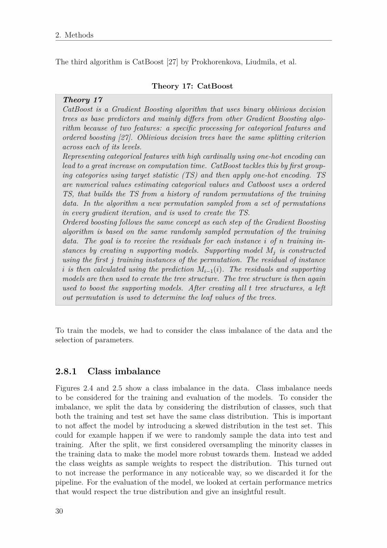
2. Methods

The third algorithm is CatBoost [27] by Prokhorenkova, Liudmila, et al.

Theory 17: CatBoost

Theory 17CatBoost is a Gradient Boosting algorithm that uses binary oblivious decisiontrees as base predictors and mainly differs from other Gradient Boosting algo-rithm because of two features: a specific processing for categorical features andordered boosting [27]. Oblivious decision trees have the same splitting criterionacross each of its levels.Representing categorical features with high cardinally using one-hot encoding canlead to a great increase on computation time. CatBoost tackles this by first group-ing categories using target statistic (TS) and then apply one-hot encoding. TSare numerical values estimating categorical values and Catboost uses a orderedTS, that builds the TS from a history of random permutations of the trainingdata. In the algorithm a new permutation sampled from a set of permutationsin every gradient iteration, and is used to create the TS.Ordered boosting follows the same concept as each step of the Gradient Boostingalgorithm is based on the same randomly sampled permutation of the trainingdata. The goal is to receive the residuals for each instance i of n training in-stances by creating n supporting models. Supporting model Mj is constructedusing the first j training instances of the permutation. The residual of instancei is then calculated using the prediction Mi−1(i). The residuals and supportingmodels are then used to create the tree structure. The tree structure is then againused to boost the supporting models. After creating all t tree structures, a leftout permutation is used to determine the leaf values of the trees.

To train the models, we had to consider the class imbalance of the data and theselection of parameters.

2.8.1 Class imbalance

Figures 2.4 and 2.5 show a class imbalance in the data. Class imbalance needsto be considered for the training and evaluation of the models. To consider theimbalance, we split the data by considering the distribution of classes, such thatboth the training and test set have the same class distribution. This is importantto not affect the model by introducing a skewed distribution in the test set. Thiscould for example happen if we were to randomly sample the data into test andtraining. After the split, we first considered oversampling the minority classes inthe training data to make the model more robust towards them. Instead we addedthe class weights as sample weights to respect the distribution. This turned outto not increase the performance in any noticeable way, so we discarded it for thepipeline. For the evaluation of the model, we looked at certain performance metricsthat would respect the true distribution and give an insightful result.

30

2. Methods

2.8.2 Parameter tuningThe scope of this project is bigger than in most machine learning projects as weinvestigate multiple targets and compare different classifiers in addition. This leavesus with not one but 15× 3 = 45 models and parameter settings to tune. Parametertuning is usually meant to be a fine tuning of the model and should not have a crucialimpact on its performance such as feature selection and engineering do. Therefore,we limited the parameter tuning to a minimum, applying grid search with between48 and 96 parameter combinations. The models vary quite a bit when it comes tothe parameters that are recommended to be considered while tuning. As LightGBMfor example uses a leaf-wise growing algorithm for constructing trees this requiresdifferent parameters to tune than algorithms with depth-wise growing algorithm. Inaddition we applied early stopping to prevent the models from overfitting on thetraining sets. The results showed a slight improvement of prediction performance.

2.8.3 Evaluation of classifier modelsAs stated earlier we want our models to perform well on non-anomalies and poorlyon anomalies.To measure the prediction performance of our models on the non-anomalies wedecided to use two variations of the evaluation metric F1-score: weighted F1 scoreand macro F1 score. The F1 score [9] was first introduced by Dice, Lee R.

Theory 18: F1 score

Theory 18For an example binary classification problem with a positive and negative class,there will be four classes that explains how good the classifications was. Thefour classes are TP (true positive), FP (false positive), TN (true negative), FN(false negative). These four classes can be found in the elements of a generatedconfusion matrix. From the elements of the confusion matrix one can obtainthe precision score which quantifies how precise a model is on the instances thatwere predicted positive. From the Equations in 2.12 give the definitions of recall(r) and precision (p).

r = TP

TP + FN, p = TP

TP + FP(2.12)

These metrics explains more about the actual predictions than just the accuracyof the classifier. The metrics have their own niche cases when used, but sincewe were not interested in just one of the metrics, we used the F1 score which isthe harmonic mean of recall and precision

F1 = 2 ∗ p ∗ rp+ r

.

31

2. Methods

In general the F1 score gives a trade-off between precision and recall and is a goodchoice for evaluation if neither is preferred for the application. The weighted F1score calculates the score for each label, that is a specific configuration setting, andbuilds the average F1 score using the number of true instances in the data set asweights. This takes the imbalance of classes into account resulting in a score thatgives a good indication for the overall prediction performance of a model. The macroF1 score however does not take the imbalance of classes into account, resulting inan average score that weights the F1 score of every label equally. We can use thisscore to see if our model is predicting well on all labels, or possibly on the labelsthat take the major part of the data. In general, we are aiming for good scores inboth metrics, but we expect that the macro F1 score will be lower than the weightedF1 score.For the evaluation of our models on the anomalies we only considered the weightedF1 score. We want to achieve a fairly poor prediction performance on this data set,preferably in absolute terms but at least relatively to the prediction performance onnon-anomalies.

2.9 Evaluation of configuration recommendationsThe main goal of our application is to increase link performance by changing config-uration settings. Therefore, we intended to compare a performance metric for initialconfiguration settings and the recommendations of our models. A part of such a per-formance metric was described in Section 2.3. Unfortunately, further performanceinformation was not available during this project. The information available wasused to investigate the possibilities to evaluate our recommendations without ap-plying them in reality. As the application of our recommendations in live networksis not possible we rely on the accessible data. However, performance data is onlyavailable for real links and their configuration settings and not for the configurationrecommendations we provide. Therefore, we tried to approximate the performancevalues for our recommendations.One way to approximate the performance metric is to find a fairly similar link fora given environment-configuration pair. We can think of an embedding space thatexpresses closeness between different environment-configuration pairs in combina-tion with a data structure that enables an efficient lookup for k nearest neighbours.Querying a new environment-configuration pair, in our case the existing link envi-ronment with its new configuration settings, will then result in finding k links thatare closest to it in terms of its characteristics. As environment and configurationsare close we would expect the operational conditions to be similar as well. Given thissimilarity we can obtain an approximation of the performance of the unknown pointby using the performance values of the k nearest links. This idea was implementedusing the cat2vec embedding, which is the same embedding used for the clusteringand is described in Section 2.4, in combination with a kd-tree as a lookup structure.The kd-tree [13] was introduced by Friedman, Bentley Finkel. In principle a kd-treeis a general form of a binary tree allowing any file to be partitioned in the mannerof a binary tree. A partition creates subfiles and also defines lower or upper boundsfor the subtrees. These boundaries create multidimensional cells in the search space

32

2. Methods

and help the nearest neighbour algorithm to ignore instances within cells that aretoo far away already, and therefore reducing the number of comparisons.The results of the nearest neighbour search in an early stage of the project weredisappointing as the closest neighbour would almost always be the initial link andtherefore resulting in a performance difference of 0. This might indicate that chang-ing some configuration settings is not good enough to land on another link. Anotherpossible explanation is that the data set is not big enough as there are no other linksclose to the combination of environmental features and the recommended configura-tion settings. For a data set with more links and a higher variance of environment-configuration combinations this approach might work. Either way this approachwas not applicable for this project and its data.

Another approach for an evaluation is the discussion of our models’ results withexperts. This can help to see whether our configuration recommendations are rea-sonable and in which ways our models can be improved. We were in an exchangewith experts from Ericsson in an earlier stage of the project but did not receiveenough feedback in a later stage.This leaves us with no final evaluation of the models for now. A number of iterationsincluding discussions and evaluations with domain experts however seems promisingand is something worth looking into in the future.

33

2. Methods

34

3Results and Discussion

The thesis work aimed to explore the possibility to apply machine learning methodsto find anomalies in microwave link configuration settings and the recommendationsto replace these settings. The available data drew us to the developed approach ofidentifying possible anomalies using clustering and a simple anomaly score and thenexcluding anomalies in the training process for models shifting towards the moreusual cases of configuration settings. The approach was implemented using the dataof two selected customers, as this data seemed the most complete and explored. Thedata set describes 12068 microwave links including several environmental and config-uration features. Through the described process of feature selection and engineeringwe ended up including 34 environmental features and 14 configuration features, suchas modulation, minimum and maximum output power and the bit-error-rate alarmthreshold. A complete list of the features and its explanations is provided in Ap-pendix B.We investigated several possibilities for different aspects of the thesis, such as differ-ent cluster algorithms and evaluations for the plausibility of our final recommenda-tions. Investigations with no positive impact were also mentioned in method Section2 but will not be considered in the presentation of the final results in this section.Derived from the assumptions about the data we define a good prediction per-formance for this particular recommendation problem as a precise prediction fornon-anomalies and a fairly poor prediction precision for anomalies. Therefore, weaim to increase the weighted F1 score and macro F1 score for non-anomalies anddecrease the weighted F1 score for anomalies. However, we consider having a goodperformance on non-anomalies more important, as we should treat the anomaliesresulting from the anomaly detection as anomaly candidates, meaning that a goodprediction on a fraction of the anomalies might be desirable as these might not beanomalies after all.

3.1 Evaluating the baselineTable 3.1 shows the averaged model evaluation over all 14 configurations for eachthe Random Forest classifier and the dummy classifier when trained on the biggerdata set of 12068 microwave links excluding the environmental features from theinflux database as this data is only available for a subset of the links. The clusteringof environmental features resulted in 55 clusters, and setting the threshold for theanomaly score to 0.01 resulted in 877 anomalies among all configuration featuresand therefore around 63 anomalies per configuration feature on average.

35

3. Results and Discussion

As already stated the possibilities to improve microwave configuration settings usingmachine learning have been unexplored until now. Therefore, we investigated thedata using a naive dummy classifier that always chooses the most dominant class inthe data set. The classes are quite unbalanced in some cases and the prediction per-formance of more complex classifiers might therefore be misleading when standingalone for themselves, as good results might be achievable when taking advantage ofthe class distributions.

F1weighted

F1macro

F1anomalies

Dummy 0.4668 0.1443 0.2954Random Forest 0.8967 0.6938 0.1865

Table 3.1: Comparing evaluation metrics of baseline models. The highlighted cellsshow the best results of the according evaluation metric according to our definitionof a good performance for our models.

The results for the dummy classifier show that even though there are configurationfeatures with very dominant classes the average prediction performance is quitepoor.We then trained the Random Forest classifier on the same data set. The RandomForest classifier clearly outperforms the dummy classifier as it shows a weighted F1score about twice as high and a macro F1 score almost 5 times as high. This showsthat the data indeed allows the application of machine learning algorithms as theRandom Forest classifier picks up meaningful relations within the data. The macroF1 score is however still quite low compared to the weighted F1 score, indicating thatthe model struggles with minority classes. This could mean that the model missesmore complex relations or simply lacks necessary features to explain the remainingvariance of the targets.The predictions on the anomaly data set show that anomaly links, according to theanomaly detection, indeed differ from other links and the Random Forest classifieris not able to predict the right configuration settings with the relations it picked upon the normal links. This might also be due to the generally lower frequencies ofconfiguration settings appearing in anomaly links.

3.2 Comparing gradient boosting classifiersAs a next step we considered more complex models with the goal to push predictionperformance further. We decided to investigate the potential of different implemen-tations of gradient boosting algorithms, namely XgBoost, LightGBM and CatBoost.We used the same data set as for the baseline models. The results of the evaluationare stated in Table 3.2.

All gradient boosting algorithms are able to outperform the Random Forest Clas-sifier as weighted F1 score and macro F1 score increase slightly. Contrary to our

36

3. Results and Discussion

F1weighted

F1macro

F1anomalies

XGBoost 0.9139 0.7476 0.3087LightGBM 0.9111 0.7376 0.2513CatBoost 0.8987 0.6906 0.2205

Table 3.2: Comparing evaluation metrics of different gradient boosting models.The highlighted cells show the best results of the according evaluation metric ac-cording to our definition of a good performance for our models.

definition of a good model performance, the F1 score for the anomaly data set in-creases as well. As already stated we focus on a good prediction performance on thenon-anomalies and should evaluate the prediction performance on anomalies withcare.Even though LightGBM and CatBoost include a special feature representation forcategorical data, as stated in Theory 17, the algorithms are not able to outperformXGBoost. The results are close and only differ in a small magnitude, which is notsurprising as the the core idea of all algorithms is the same and an improvement ofperformance becomes harder when getting closer to 100%. XGBoost seems to workbest for our application and we therefore proceeded to investigate possible improve-ments of this model.

3.3 Recommendation results from XGBoostTable 3.3 shows the top 10 recommendations resulting from the XGBoost modelthat was evaluated in this step and is sorted by the anomaly scores. Regarding ourconsiderations about the anomaly score, a lower score indicates a lower likelihoodfor the configuration setting to be right. However, it should not be interpreted as anabsolute probability but rather be considered in relative terms. Such a list of recom-mendations represents the final result of our application. The table shows differentconfiguration setting changes for specific microwave links. Their true link ids werereplaced by consecutive numbers as we are not allowed to publish provider-specificinformation.Evaluating the value changes is difficult as incorrect configuration settings are notlabeled, identifying true wrong configuration settings in a different way is very diffi-cult and other possible options as described in Section 2.9 failed because of missingdata and participation of domain experts. The right choice of configuration settingsis influenced by many factors, such as the environmental features, which we hadaccess to and integrated in the model, and other information such as restrictions re-sulting from a network planning process or a provider in general, e.g. the frequenciesa provider has the license for. The model might pick up some of this informationimplicitly, but the results from Table 3.2 already show that there seems to be aninformation gap as some configuration settings are mispredicted. We further inves-tigated this by considering additional features for the models. The results are shown

37

3. Results and Discussion

in the following section.

anomalyscore id configuration old new

0.000012 1 modulation 512 qam 4096 qam0.000039 2 input_alarm_threshold -56.7 -92.70.000045 3 modulation 512 qam 4096 qam0.000123 4 atpc_max_output_power 17.33 25.330.000128 5 max_output_power 25.5 23.00.000128 6 modulation 4 qam 4096 qam0.000150 7 input_alarm_threshold -56.7 -92.70.000150 8 input_alarm_threshold -56.7 -92.70.000150 9 input_alarm_threshold -56.7 -92.70.0001504 10 input_alarm_threshold -56.7 -92.7

Table 3.3: Top 10 recommendations taken from the XGBoost Classifier trainedon the big data set. Old values show the configuration settings present in thedata and new values show the recommendations resulting from our models. E.g.recommendations for links 5,6 and 7 suggest a change to a higher QAM modulation,which allows a higher capacity for the link but also increases the chance for errorsduring transmission.

3.4 Evaluating the impact of additional environ-mental features

The previous section of the results are based on models that only consider environ-mental features from the impala data base. As a next step we tried to make use ofa) features from a time series database of an operation condition classifier and b) ofpossible dependencies among configuration features. A list of all features, their ex-planations and where they come from is provided in Appendix B. As already statedin Section 2.1.1 the scope of the classification application is limited to a subset ofthe links. We obtained classification data for 6729 out of 12068 links. The newfeatures provide information about what influences a link’s operation condition andadditional information about the location of links. The results for training XGBoostclassifiers on the new data set are presented in Table 3.4, again showing the aver-age scores among the classifiers for all configuration features. The first row showsthe results for training the classifiers on the subset without the additional features.This is necessary to observe the impact of additional features as the subset of linksin this data set is specific as a majority of these links are placed in urban areas.

38

3. Results and Discussion

The second row shows the results of XGBoost classifiers trained on the same dataset including the additional features from the Influx database. In the last row, weincluded all other configuration features as environmental features in addition to thefeatures from the influx database. A detailed list of evaluation results when usingthese additional features can be seen in Table D.3 in the Appendix D.

F1weighted

F1macro

F1anomalies

0.9293 0.6961 0.3948+ influx 0.948 0.7544 0.3501+ configurations 0.9745 0.8733 0.5384

Table 3.4: Comparing the averages of evaluation metrics for a subset of the dataset. In two steps we added features from an operation condition classification andremaining configuration features as additional environmental features.

Adding features from an operation condition classifier

Adding the features from the influx database results in 30 clusters and a total of338 anomalies, therefore around 24 for each configuration feature on average. Theadditional features push our models a little bit further as weighted F1 score andmacro F1 score increased. To what extent these features have an impact can beinvestigated using feature importance plots. All feature importance plots are givenin Appendix E. An example is provided by Figure 3.1. We used the feature impor-tance score gain, indicating the contribution of a feature on decisions in the decisiontrees relatively to all other features. When looking at the lower F1 score for theanomalies we have to keep in mind that the new features are also influencing theclustering and therefore the anomaly detection.

It is not surprising that features like the hop length have an impact on the modelperformances, as this is information that is also considered when configuring mi-crowave links in the first place. However, information about the operation conditionis unknown at that point but still shows a relation to the configuration settings.This means that a link whose operation condition is affected in a certain way ,e.g.by wind, tends to be configured differently. As the model picks up a relation tomeaningful configuration settings for different operation conditions, configurationrecommendations might become more meaningful. Again, this is something we can-not evaluate at this point.

Considering dependencies between configurations

We went one step further and considered possible dependencies between configura-tion settings. This means that a setting for one configuration feature might affect

39

3. Results and Discussion

Figure 3.1: Feature importance plot for the configuration feature min output powerfor automatic transmission power control. This plot gives an example of how theadditional features from the influx database have an impact on the decision mak-ing. Such additional features are: decision_restart, decision_maintenance, deci-sion_obstruction and hop_length. The feature importance values speak in relativeterms, expressing a feature’s influence on decisions in decision trees compared to allother features.

the configuration setting of a different configuration feature. We already exploreddirect correlations between configuration settings using Cramer’s V and associa-tion matrices in Section 2.2 and removed configuration features from our scope thatseemed redundant. An association matrix for the configuration features is given inAppendix A.2. The remaining configuration features show rather low associationsbetween each other, but there might be more complex relations between them. Acombination of surrounding configuration settings might then help to predict thecorrect configuration setting for the configuration feature the model is trying to pre-dict. Therefore we included the surrounding configuration features when trainingthe models. However we did not consider these features for the clustering.Including other configuration features as environmental features pushes our modelseven further as weighted F1 score and specially macro F1 score increase one moretime by around 0.025 and 0.086. Other configurations in fact seem to have a quitebig impact on some of the configuration features as the prediction performance forsome configuration features increases. This can be seen in Table D.3 in the Ap-pendix. E.g. the models for the configuration features max_output_power andchannel_spacing do not improve much when adding the configuration features tothe context of a link whereas the weighted F1 score for the model of feature modu-lation improves by another 0.12.

The results from Table 3.4 and the feature importance plots from Appendix E showthat some configuration features are quite dependent on other configuration features.

40

3. Results and Discussion

anomalyscore id conf old new

0.000141 11 ber_alarm_threshold 10eMinus3 10eMinus60.000247 12 max_output_power 17.0 21.00.000286 6 modulation 4 qam 4096 qam0.000297 4 atpc_max_output_power 17.333333 25.3333330.000309 13 modulation 512 qam 2048 qam light0.000434 14 max_output_power 19.0 23.00.000461 15 ber_alarm_threshold 10eMinus3 10eMinus60.000461 16 ber_alarm_threshold 10eMinus3 10eMinus60.000461 17 ber_alarm_threshold 10eMinus3 10eMinus60.000581 18 max_output_power 19.0 20.0

Table 3.5: Top 10 recommendations taken from the XGBoost Classifier trained onthe smaller data set with influx data and configuration features as environment

We therefore conclude that respecting these dependencies between configuration fea-tures is crucial for a recommendation task as of this thesis work. The final modelsshow fairly good prediction performance on the normal links. The fairly good pre-diction performance of 0.5534 on the anomalies indicates, that there are possibly farless misconfigurations in the data set then we expected. We could therefore considerto lower the threshold of the anomaly detection.We finally have a look at the top 10 recommendations of these models in Table 3.5.We can see that recommendations for id 1 and 9 are the same as from the modelswithout any additional features. Again, we cannot say much about the reasonabilityand potential performance improvement of our recommendations as we lack a wayto evaluate them.

41

3. Results and Discussion

42

4Conclusion

In this thesis we investigated the possibilities to configure microwave links with adata-driven approach. We were specially interested in identifying incorrect config-urations and providing suitable configuration recommendations for these cases. Weassumed that the number of incorrect configuration settings is low for the networkwe looked into. Incorrect configuration settings would then appear rarely and couldbe identify as anomalies. We implemented a machine learning approach that firstidentifies anomaly candidates for a certain configuration feature, secondly trains amodel excluding these anomaly candidates and at last provides recommendationsfor the anomaly candidates. This resulted in an anomaly detection and classifiermodel for each configuration feature in scope.To locate the anomalies we first tried applying anomaly detection methods on theenvironmental features and the chosen configuration setting. This did not work as alot of variance came from the environmental features. Instead, we used the density-based clustering algorithm HDBSCAN to cluster the environmental features. Asthe clustering of microwave links according to their environmental features is anunsupervised problem, it remained difficult to tune and evaluate the clustering untilthe end. The final clustering was obtained from observing DBCV score, SilhouetteCoefficient and the number of clusters and anomalies. These four values helped tofind a clustering that appears to fit the data.Microwave links within the resulting clusters were similar in their environmental fea-tures. We empirically developed two anomaly detection scores to point out atypicalconfiguration settings for each cluster. The scores are mainly based on frequenciesof configuration settings within a cluster and within the total of all microwave links.Since there was no way to evaluate the anomaly detections we simply chose one ofthem.

The results show that machine learning models are a viable option to help findsuitable configurations for microwave links. The first data set consisted of infor-mation for 12068 microwave links and we excluded about 63 anomalies on averageamong all configuration features. Environmental features consisted mostly of hard-ware and software information. The models picked up relevant relationships andwere able to give fairly good results overall. We trained different Gradient Boostingalgorithms on this data set. XGBoost outperformed LightGBM and CatBoost andwe continued to use XGBoost in the next steps.The prediction for less frequent configuration settings seemed more difficult for themodels in most cases. We tried to improve the models adding additional envi-ronmental features. The prediction performance increased when adding additional

43

4. Conclusion

location information and averaged information about operation conditions. In a nextstep we considered dependencies between configuration features and therefore usedother configuration features as environmental features. The prediction performanceincreased once more, proving that there are dependencies between configuration set-tings. The final set of models had an average weighted F1 score of 0.9744 and andaverage macro weighted F1 score of 0.8692. We believe that there is more informa-tion respected in the original configuration process. Such information could pushour models once more, leading to a better prediction and a better reliability whendetecting anomalies.

Applying the trained models on the sets of anomaly candidates showed a lowerprediction performance. This was excepted as we desired our models to predictgood or common configuration settings and not uncommon settings that might beincorrect. We interpreted the mispredictions of our models as configuration recom-mendations. The evaluation of these results is difficult and we are left with a lot ofuncertainty for the reliability of the anomaly detection and the quality of our config-uration recommendations. This is due to the unsupervised nature of the problem aswe do not know which configurations are in fact incorrect and indirect ways to checkthis, e.g. evaluating the performance of microwave links that might be configuredincorrectly, were not possible in the scope of this thesis work.Our approach shows that data-driven configuration for microwave networks and therecommendation of more suitable configuration settings is in principle possible. Thisis first investigation of the problem and configuration predictions of our models needto be shifted into the right direction and be restricted by the boundaries of a net-work’s reality. This requires additional meaningful features and a reliable evaluationprocess for the anomaly detection and configuration recommendations.

44

5Future Work

At the end of this thesis we are left with many interesting opportunities to buildon this thesis work. Some of them acknowledge the limitations of the project andtry to break them, others show different approaches for further investigations of theproblem. The main ideas for these opportunities are stated in the following sections.

5.1 Utilization of performance dataThe main point that needs to be investigated is the evaluation of the steps in thepipeline. Our initial idea was to create a performance function that would describethe overall performance for a microwave link over a given interval. Since we werenot able to construct the function, further investigation would be necessary. Wecould construct such a function for a bigger data set and richer performance data.The design of the function could be based on evaluation from visualization tools tounderstand how the parameters changes the performance score. With a performancefunction certain steps in the pipeline could have been quite different.

There could have been an evaluation for the anomaly detection. If we assumethat misconfigurations have a less than average performance score over a long in-terval, then this should be reflected in the identified anomalies. For example, if wetake the average performance scores of the anomalous and normal microwave links,we would expect the average score of the normal links to be larger. Therefore, agood evaluation of the anomaly detection is the difference between the two aver-ages, where a large difference indicates that the method has identified anomalieswell. With this evaluation we could both tune the anomaly detections and selecteda superior method from our two candidates, instead of simply selecting one. Also,with a performance function we could have added weights for the models based onthe performance scores. This could have been a great addition to the prediction byplacing emphasis on microwave links with a low performance score.

Finally, we could have properly evaluated the result of the pipeline. Once we geta recommendation for a configuration setting we can see the difference between theold performance value and the estimated performance value from similar microwavelinks. Similar microwave links can be found with nearest neighbour algorithms forthe configuration and environment space that all the microwave links span. Theperformance difference makes ranking the recommendations possible in terms ofthe largest performance increase. The ranking of recommendations based on per-

45

5. Future Work

formance difference is more insightful than ranking based on the most anomalous,because the performance score would be based on live data. With the highest rankedrecommendations, these would be the most interesting ones to analyze further.

5.2 Investigating different networksOur results are based on the data of a network who’s configuration settings havebeen quite optimized already. It would be interesting to see how our approachperforms on the data of network that has not been optimized. This brings up theopportunity for a knowledge transfer, as we could train our models on optimizednetworks and provide recommendations for non-optimized networks.

5.3 Investigating more data sourcesThe selection of meaningful features took a large part of this thesis already. However,our feature selection does not explain all of the configuration settings’ varianceyet. We suspect that the configuration process is guided by additional data, suchas certain boundaries for power levels and frequencies. Such additional planninginformation could help to make predictions of our models more reliable and thereforeidentify anomalies with more certainty. The usage of the available data sources forthis project were just a first step and utilizing more meaningful data sources canpush our models further.

5.4 Applying constraints on the recommendationsCurrently, the recommendations do not have any rules to the values it recommends.For the recommendations to be insightful they need to be constrained within rangesof acceptable values. The constraints could be applied in two different places, fil-tering on the recommendations and applying weights to configuration settings. Thefirst constraint could be applied on the final list of recommendations, by creating arule-based system that filters out all values that can not be configured. The latterconstraint could be applied by investigating if the model needs a bias towards acertain subset of the configuration setting’s value range, such that it rarely recom-mends the values outside of the subset. These constraints would be very useful ifthe recommendations should be considered for production, so that no false settingsare applied.

5.5 Wrapper approachThe three gradient boosting algorithms that we used find different kinds of patternsin the data because of their differing architecture. Since all methods did well on thedata, it might be worth investigating what a wrapper around the three classifierswould do. Then, a majority vote could be taken from their respective output andwe would see how that would affect the predictions.

46

5. Future Work

5.6 Neural Network ApproachSince we were investigating the feasibility of utilizing machine learning approacheson the unexplored data, we wanted the models to be simple. Based on the result weknow that machine learning is viable and so the question is how would the resultchange if a more complex model were used instead. One idea that we had was touse a neural network instead of decision trees. Neural networks are good at cap-turing the underlying relationship between features and targets, and since there isstill room for improvement based on the results, this could be interesting to lookinto. Additionally, if a performance function were given, we would be able to findan optimal configuration by redefining the problem as:

For a neural network approach we want to approximate a performance surface overall possible context vectors y and configuration vectors x that is based on the valuesof the performance function. First, we would train a neural network by using thevector [x0, y0] as input and the respective performance value as output. Once themodel is trained, to find the optimal configuration is to run the network on everycombination of [x, y = y0] and assign the configuration vector that corresponds tothe highest value that the network will output. This could be feasible if the numberof permutations of the configuration vector is not too large. The formulation of thisapproach was inspired by the work of Haigh et al. [15]. They used a neural networkto approximate a performance surface for devices in mobile ad hoc networks basedon configurations and environmental information.

The two main reasons to why this approach was not used was that we wanted asimple machine learning algorithm to explore the data set, and that considering thedata size we would not be able to design a deep network since there was not muchdata to train on.

47

5. Future Work

48

Bibliography

[1] Andreas Adolfsson, Margareta Ackerman, and Naomi C Brownstein. To cluster,or not to cluster: How to answer the estion. TKDD ‘17, Halifax, Nova Scotia,Canada ACM, 2016.

[2] Andreas Adolfsson, Margareta Ackerman, and Naomi C Brownstein. To cluster,or not to cluster: An analysis of clusterability methods. Pattern Recognition,88:13–26, 2019.

[3] Mihael Ankerst, Markus M Breunig, Hans-Peter Kriegel, and Jörg Sander. Op-tics: ordering points to identify the clustering structure. ACM Sigmod record,28(2):49–60, 1999.

[4] A. Awada, B. Wegmann, I. Viering, and A. Klein. Optimizing the radio networkparameters of the long term evolution system using taguchi’s method. IEEETransactions on Vehicular Technology, 60(8):3825–3839, Oct 2011.

[5] Amit Banerjee and Rajesh N Dave. Validating clusters using the hopkins statis-tic. In 2004 IEEE International conference on fuzzy systems (IEEE Cat. No.04CH37542), volume 1, pages 149–153. IEEE, 2004.

[6] Ricardo JGB Campello, Davoud Moulavi, and Jörg Sander. Density-basedclustering based on hierarchical density estimates. In Pacific-Asia conferenceon knowledge discovery and data mining, pages 160–172. Springer, 2013.

[7] Tianqi Chen and Carlos Guestrin. Xgboost: A scalable tree boosting system.In Proceedings of the 22nd acm sigkdd international conference on knowledgediscovery and data mining, pages 785–794, 2016.

[8] Harald Cramér. Mathematical methods of statistics, volume 43. Princetonuniversity press, 1999.

[9] Lee R Dice. Measures of the amount of ecologic association between species.Ecology, 26(3):297–302, 1945.

[10] Chris Ding and Xiaofeng He. K-means clustering via principal componentanalysis. In Proceedings of the twenty-first international conference on Machinelearning, page 29, 2004.

[11] Rémi Domingues, Maurizio Filippone, Pietro Michiardi, and Jihane Zouaoui.A comparative evaluation of outlier detection algorithms: Experiments andanalyses. Pattern Recognition, 74:406–421, 2018.

[12] Martin Ester, Hans-Peter Kriegel, Jörg Sander, Xiaowei Xu, et al. A density-based algorithm for discovering clusters in large spatial databases with noise.In Kdd, volume 96, pages 226–231, 1996.

[13] Jerome H. Friedman, Jon Louis Bentley, and Raphael Ari Finkel. An algorithmfor finding best matches in logarithmic expected time. ACM Trans. Math.Softw., 3(3):209–226, September 1977.

49

Bibliography

[14] David Guthrie, Ben Allison, Wei Liu, Louise Guthrie, and Yorick Wilks. Acloser look at skip-gram modelling. In LREC, pages 1222–1225, 2006.

[15] K. Z. Haigh, S. Varadarajan, and Choon Yik Tang. Automatic learning-basedmanet cross-layer parameter configuration. In 26th IEEE International Con-ference on Distributed Computing Systems Workshops (ICDCSW’06), pages84–84, July 2006.

[16] John A Hartigan, Pamela M Hartigan, et al. The dip test of unimodality. Theannals of Statistics, 13(1):70–84, 1985.

[17] Tin Kam Ho. Random decision forests. In Proceedings of 3rd internationalconference on document analysis and recognition, volume 1, pages 278–282.IEEE, 1995.

[18] Brian Hopkins and John Gordon Skellam. A new method for determining thetype of distribution of plant individuals. Annals of Botany, 18(2):213–227, 1954.

[19] H. Hu, J. Zhang, X. Zheng, Y. Yang, and P. Wu. Self-configuration and self-optimization for lte networks. IEEE Communications Magazine, 48(2):94–100,2010.

[20] C. Jiang, H. Zhang, Y. Ren, Z. Han, K. Chen, and L. Hanzo. Machine learningparadigms for next-generation wireless networks. IEEE Wireless Communica-tions, 24(2):98–105, 2017.

[21] Guolin Ke, Qi Meng, Thomas Finley, Taifeng Wang, Wei Chen, Weidong Ma,Qiwei Ye, and Tie-Yan Liu. Lightgbm: A highly efficient gradient boostingdecision tree. In I. Guyon, U. V. Luxburg, S. Bengio, H. Wallach, R. Fergus,S. Vishwanathan, and R. Garnett, editors, Advances in Neural InformationProcessing Systems 30, pages 3146–3154. Curran Associates, Inc., 2017.

[22] M. G. Kibria, K. Nguyen, G. P. Villardi, O. Zhao, K. Ishizu, and F. Kojima. Bigdata analytics, machine learning, and artificial intelligence in next-generationwireless networks. IEEE Access, 6:32328–32338, 2018.

[23] Fei Tony Liu, Kai Ming Ting, and Zhi-Hua Zhou. Isolation forest. In 2008Eighth IEEE International Conference on Data Mining, pages 413–422. IEEE,2008.

[24] Leland McInnes, John Healy, and Steve Astels. hdbscan: Hierarchical densitybased clustering. The Journal of Open Source Software, 2(11), mar 2017.

[25] Tomas Mikolov, Ilya Sutskever, Kai Chen, Greg S Corrado, and Jeff Dean.Distributed representations of words and phrases and their compositionality.In Advances in neural information processing systems, pages 3111–3119, 2013.

[26] Davoud Moulavi, Pablo A Jaskowiak, Ricardo JGB Campello, Arthur Zimek,and Jörg Sander. Density-based clustering validation. In Proceedings of the2014 SIAM international conference on data mining, pages 839–847. SIAM,2014.

[27] Liudmila Prokhorenkova, Gleb Gusev, Aleksandr Vorobev, Anna VeronikaDorogush, and Andrey Gulin. Catboost: unbiased boosting with categorical fea-tures. In S. Bengio, H. Wallach, H. Larochelle, K. Grauman, N. Cesa-Bianchi,and R. Garnett, editors, Advances in Neural Information Processing Systems31, pages 6638–6648. Curran Associates, Inc., 2018.

50

Bibliography

[28] Peter J Rousseeuw. Silhouettes: a graphical aid to the interpretation and vali-dation of cluster analysis. Journal of computational and applied mathematics,20:53–65, 1987.

[29] Robert Tibshirani, Guenther Walther, and Trevor Hastie. Estimating the num-ber of clusters in a data set via the gap statistic. Journal of the Royal StatisticalSociety: Series B (Statistical Methodology), 63(2):411–423, 2001.

[30] U. Turke and M. Koonert. Advanced site configuration techniques for auto-matic umts radio network design. In 2005 IEEE 61st Vehicular TechnologyConference, volume 3, pages 1960–1964 Vol. 3, May 2005.

[31] M. N. ul Islam, R. Abou-Jaoude, C. Hartmann, and A. Mitschele-Thiel. Self-optimization of antenna tilt and pilot power for dedicated channels. In 8thInternational Symposium on Modeling and Optimization in Mobile, Ad Hoc,and Wireless Networks, pages 196–203, 2010.

[32] Laurens Van Der Maaten, Eric Postma, and Jaap Van den Herik. Dimension-ality reduction: a comparative. J Mach Learn Res, 10(66-71):13, 2009.

[33] Ying Wen, Jun Wang, Tianyao Chen, and Weinan Zhang. Cat2vec: Learningdistributed representation of multi-field categorical data. 2016.

51

Bibliography

52

AAppendix 1: Association matrices

Using the Cramer’s V we calculate and plot an association matrix for all possiblecandidates of environmental features. The matrix is similar to a correlation ma-trix, where a higher number, or warmer color, indicates an association between twofeatures, meaning that the values of these features are more likely to come in pairs.

Figure A.1: Heatmap showing associations between environmental features.

I

A. Appendix 1: Association matrices

The same goes for the pre-selection of configuration candidates.

Figure A.2: Heatmap showing associations between configuration features.

II

A. Appendix 1: Association matrices

The association matrix between environmental features and configuration visualizeshow certain environmental features explain variance in some configurations directly.

Figure A.3: Heatmap showing associations between pairs of environmental andconfiguration features.

III

A. Appendix 1: Association matrices

IV

BAppendix 2: Feature explanations

Table B.1 lists all considered environmental features and a short explanation of theirnames.

feature name explanation

ammposition_r Physical position of the radio within the rackfamily_r Name for radio familyhp_r Flag for high power radioorientation_r Indicates whether the radio is operating on

the lower or higher part of the radio family’sfrequency.

version_r Version of the radioactivesw_r Software used for the active operations of the

radiotypeofunit_m Type of modem unitversion_m Version of the modemactivesw_m Software used for the active operations of the

modemswproductnumber_m Product number of the software used for the

modemtypeofswunit_m Type off the software unit for the modemtypeofunit_n Type of unit of the node processor unitversion_n Version of the node processor unitactivesw_n Software used for the active operations of the

node processor unittypeofunit_f Type of unit of the fan unitkg_class Climate classification according to Köppen-

Geiger. Is based on location of a links nearend.

customer Name of the customer. Some configurationsseem to be customer-specific.

V

B. Appendix 2: Feature explanations

atpc_selected_input_power_far Desired input power for the receiver of the farend node this link. The Automatic TransmitPower Control will try to adjust the transmitpower to achieve this input power.

base_rx_frequency Frequency for down-conversion in the receiverof the link.

base_tx_frequency Frequency of transmit carrier of the linkmax_packet_link_capacity Maximum for the packet link capacity of a linkfreq_index_r Index for frequency sub-bandtemperature_ra1 -decision_maintenance Percentage of time the link’s signal has been

classified as being under by maintenancedecision_multipath Percentage of time the link’s signal has been

classified as being affected by multipathdecision_no_data Percentage of time no classification data was

availabledecision_normal Percentage of time the link’s signal was was

classified as normaldecision_obstruction Percentage of time the link’s signal has been

classified as being affected by obstructiondecision_precipitation Percentage of time the link’s signal has been

classified as being affected by precipitationdecision_restart Percentage of time the link’s signal has been

classified as being restarteddecision_wind Percentage of time the link’s signal has been

classified as being affected by windcurrent_step_number_rx -current_step_number -hop_length Distance between near and far end of the link

measured in kilometers

Table B.1: List of explanations for environmental features

Table B.2 lists all considered configuration features and a short explanation of theirnames.

feature name explanation

packet_link_capacity Current packet link capacity

VI

B. Appendix 2: Feature explanations

input_alarm_threshold An alarm goes off when the input power goes belowthe threshold level

atpc_min_output_power Minimum output power for the Automatic TransmitPower Control (atpc). Is measured in decibels (dB).

atpc_max_output_power Maximum output power for the Automatic TransmitPower Control (atpc). Is measured in decibels (dB).

max_output_power Maximum output power of the microwave transmit-ter. If the maximum output power is bigger thanthe minimum output power the Automatic Trans-mit Power Control (atpc) is activated. Is measuredin decibels (dB).

min_output_power Minimum output power of the microwave transmit-ter. If the minimum output power is smaller thanthe maximum output power the Automatic Trans-mit Power Control (atpc) is activated. Is measuredin decibels (dB).

e1_number -tx_freq Frequency for the transmitter of the microwave node.

IS measured in Herz.channel_spacing Bandwidth the signal is allowed to occupytraffic_type Traffic type, like ETH or PDHber_alarm_threshold An alarm goes off when the bit-error-rate exceeds

the threshold leveltx_oper_status -modulation modulation method for information transmission,

like qam 4 or qam 512max_modulation When adaptive modulation is enabled this describes

the maximum for the adaption

Table B.2: List of explanations for configuration features

VII

B. Appendix 2: Feature explanations

VIII

CAppendix 3: Clustering

Figure C.1: Plot of a dendogram that illustrates the hierarchy of connected com-ponents. The y-axis consists of the mutual reachability distance and the color cor-responds to the log of the number of points. To divide the data into clusters, aparameter ε is needed for the algorithm. With a given ε a horizontal line is drawnin the plot and all the hierarchies below the line are divided into clusters and thedata above the line is returned as a noise cluster

IX

C. Appendix 3: Clustering

Figure C.2: Plot of a condensed cluster tree where the colors correspond to theamount of points and the y-axis represents the λ value which is defined as λ = 1

d,

where d is the mutual reachability distance. For this plot, one can see that there wasthree times when the two splits had more points than a given min_cluster_size,which corresponds to the three rectangular shapes on top of the lines. There wasalso one time when the splits were both lower than min_cluster_size, which canbe seen in the final split to the right, where there was two small blue shapes underthe line

X

C. Appendix 3: Clustering

Figure C.3: For the synthetic data that can be seen in the top-left plot that has alabel (blue,red and green), we observe how the reachability-plot (bottom plot) canbe visualized from the top-right plot (constructed spanning tree). Since this data iseasily clusterable, one can see in the reachability-plot that there are distinct outliers(marked in yellow) that separates the valleys in between. One can think that thedeeper a valley is, the tighter the cluster. For this example everything that gets ahigher reachability score than 0.1 is assigned as noise.

Figure C.4: Graph showing the gap statistic over number of clusters. The red dotrepresents the ideal amount of clusters based on the gap value.

XI

C. Appendix 3: Clustering

XII

DAppendix 4: Complete result

tables

This appendix includes tables with more detailed evaluations of the results fromsection 3. The tables show the evaluation metrics every model.

Table D.1 refers to section 3.1 where dummy and Random Forest classifier wereevaluated.

Table D.2 refers to section 3.2 where different gradient boosting models were trainedand evaluated.

Table D.3 refers to section 3.4 where XGBoost classifiers were trained on a subsetof the data set, adding data from an influx database and configuration features asenvironmental features in two steps.

XIII

D. Appendix 4: Complete result tables

dummy

randomforest

configurationF1weighted

F1macro

F1anomalies

F1weightedF1macro

F1anomalies

packet_link_

capacity0.1294

0.02360.4891

0.75210.6213

0.1833input_

alarm_threshold

0.48140.0641

0.64770.904

0.39980.0185

atpc_min_

output_power

0.45010.03

0.02740.7866

0.44630.1132

atpc_max_

output_power

0.2790.0248

0.3540.7885

0.44210.0411

max_

output_power

0.05040.014

0.05770.9114

0.83540.0392

min_

output_power

0.89370.1926

0.27271.0

1.00.7159

e1_num

ber0.9631

0.19750.0

0.97560.447

0.0tx_

freq0.0226

0.01120.2105

0.99880.9978

0.7113channel_

spacing0.5257

0.15910.8986

0.98950.863

0.3155traffi

c_type

0.96190.329

0.00.9756

0.64040.0

ber_alarm

_threshold

0.64870.43

0.00.9112

0.87880.1509

tx_oper_

status0.9015

0.48280.0606

0.96760.8557

0.0606modulation

0.09470.0244

0.65380.6876

0.53710.1099

max_

modulation

0.13320.0378

0.4630.9055

0.74860.1519

average0.4668

0.14430.2954

0.89670.6938

0.1865

Table

D.1:

Evaluationofour

baselinemodels:

Dum

myClassifier

andRandom

ForestClassifier,see

section3.1.

XIV

D. Appendix 4: Complete result tables

XGBoost

LightGBM

CatB

oost

configurationF1weighted

F1macro

F1anomalies

F1weightedF1macro

F1anomalies

F1weightedF1macro

F1anomalies

packet_link_

capacity0.8

0.74440.2538

0.7760.685

0.2620.743

0.62530.1709

input_alarm

_threshold

0.90540.4005

0.03120.9128

0.43550.0507

0.90440.3934

0.0atpc_

min_

output_power

0.84140.6097

0.06760.8403

0.59060.0806

0.79130.3966

0.0702atpc_

max_

output_power

0.82520.5738

0.03640.8127

0.54470.0189

0.77710.4033

0.0564max_

output_power

0.92320.8572

0.03380.9182

0.85650.0324

0.90130.8262

0.033min_

output_power

1.01.0

0.71591.0

1.00.5671

1.01.0

0.796e1_

number

0.97710.4986

0.00.9754

0.45290.0

0.97560.4659

0.0tx_

freq1.0

1.01.0

1.01.0

1.01.0

1.01.0

channel_spacing

0.98930.8788

0.59650,9898

0,89470,2948

0.9880.8465

0.3155traffi

c_type

0.97710.6839

0.00,9761

0,63250.0

0.97650.6477

0.0ber_

alarm_threshold

0.92110.8931

0.15090,9139

0,88320,25

0.90880.8762

0.1852tx_

oper_status

0.96720.8541

0.06250,9696

0,86970,0606

0.97090.8757

0.0606modulation

0.73140.5669

0.60870,7307

0,56220,193

0.71890.5108

0.1435max_

modulation

0.93560.9047

0.76430,9409

0,91820,7079

0.92550.8013

0.2559average

0.91390.7476

0.30870,9112

0,73760,2513

0.89870.6906

0.2205

Table

D.2:

Evaluationofdifferent

gradienboosting

algorithms:

XGBoost,LightG

BMand

Catboost.

Seesection

3.2.

XV

D. Appendix 4: Complete result tables

noinflux

influxinflux

andconfigurations

configurationF1weighted

F1macro

F1anomalies

F1weightedF1macro

F1anomalies

F1weightedF1macro

F1anomalies

packet_link_

capacity0.8237

0.66790.3177

0.89790.82

0.48120.924

0.84540.4763

input_alarm

_threshold

0.94250.3791

0.00.9485

0.33480.0

0.97240.4044

0.0atpc_

min_

output_power

0.92820.5965

0.14810.9649

0.85920.1429

0.9940.9862

0.8926atpc_

max_

output_power

0.89480.7102

0.42180.9407

0.86570.6031

0.97670.9755

0.889max_

output_power

0.95830.8717

0.2080.9643

0.92190.0364

0.97910.9723

0.0364min_

output_power

1.01.0

1.01.0

1.099.0

0.99930.9965

99.0e1_

number

0.97560.2479

0.00.9744

0.24770.0

0.9950.5642

0.0tx_

freq1.0

1.00.9559

0.99930.9994

0.87390.9993

0.9980.8739

channel_spacing

0.99930.9985

1.01.0

1.00.8907

1.01.0

0.8907traffi

c_type

0.9730.4953

99.00.975

0.561899.0

1.01.0

99.0ber_

alarm_threshold

0.91830.8941

0.00.9282

0.90710.2222

0.9620.9504

0.2222tx_

oper_status

0.96470.5888

0.00.9647

0.58880.0

0.99260.9323

0.6154modulation

0.69190.4391

0.44450.7637

0.54470.2007

0.870.636

0.7065max_

modulation

0.94030.8565

0.6360.9504

0.91010.7504

0.97850.965

0.8577average

0.92930.6961

0.39480.948

0.75440.3501

0.97450.8733

0.5384

Table

D.3:

EvaluatingXGBoost

classifieron

asubset

ofdatawith

andwithout

influxdata

andconfiguration

featuresas

environ-ment.

Seesection

3.4.

XVI

EAppendix 5: Feature importance

plots

The following plots show the gain feature importance for every XGBoost model re-sulting from the run described in section 3.4. The gain feature importance describesthe impact of a feature in the decision making of a model compared to all otherfeatures. The values should therefore be interpreted relatively to the other values.

(a) maximum output power of automatictransmit power control

(b) minimum output power of automatictransmit power control

XVII

E. Appendix 5: Feature importance plots

(c) alarm threshold for the bit-error-rate (d) channel spacing

(e) e1 number (f) alarm threshold for input signal

XVIII

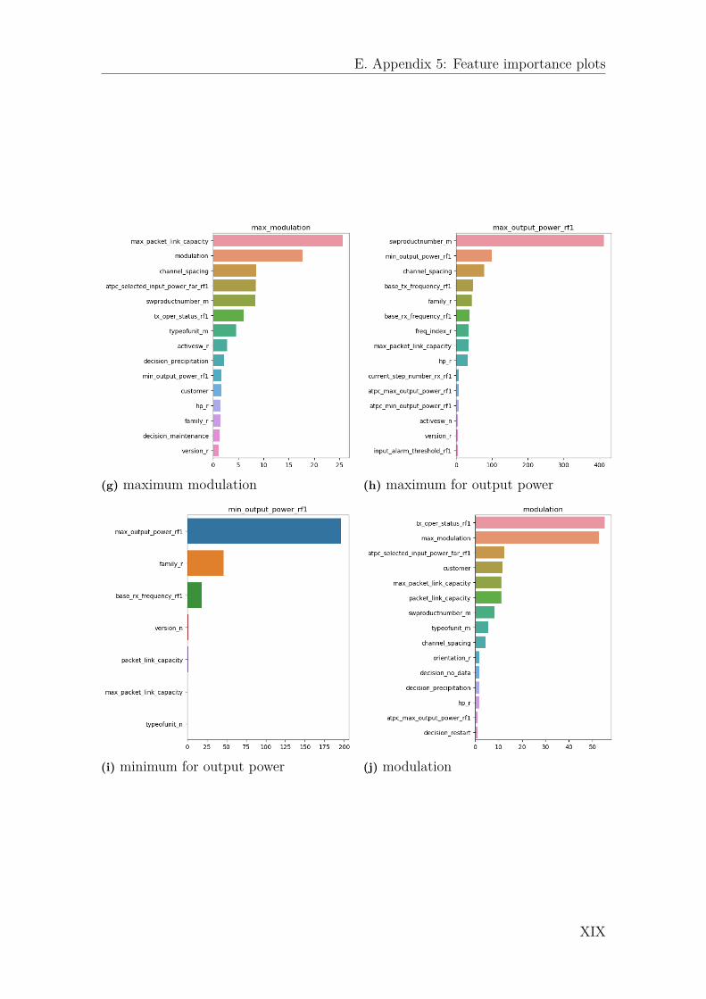
E. Appendix 5: Feature importance plots

(g) maximum modulation (h) maximum for output power

(i) minimum for output power (j) modulation

XIX

E. Appendix 5: Feature importance plots

(k) packet link capacity (l) traffic type

(m) tx frequency (n) tx operation status

Figure E.-2: Feature importance plots for all models (one model for each configu-ration feature

XX