Das House-Kapital: A Long Term Housing & Macro … House-Kapital: A Long Term Housing & Macro Model....

Das House-Kapital: A Long Term Housing & Macro Model

Volker Grossmann (University of Fribourg, CESifo, IZA, CReAM)

Thomas Steger (Leipzig University, IWH, CESifo)

European Summer Symposium in International Macroeconomics (ESSIM) 2017

Economic Development in Eastern Germany 2

1. Introduction – Motivation

Long-Term, Time-Series Data Housing wealth (Piketty & Zucman, QJE 2014) (data)

• Largest private wealth component • As share of private wealth: US 44%, UK 57% (in 2010) • Growing over time more than income (housing wealth-income ratio)

House and land prices (Knoll, Schularick & Steger, AER 2017) (data) • On average in major OECD countries, house prices tripled since 1950 • Even larger increases of land prices

Long-Term Research Questions Future evolution of housing wealth-income ratio, house prices and land prices?

How does secular increase in housing demand affect distribution of wealth?

Dynamic consequences of rent control for inequality and welfare?

Dynamic consequences of housing property taxation?

Macroeconomic effects of zoning regulations and building restrictions?


1. Introduction – Model Features

Two-sector Ramsey Growth Model Non-residential sector Housing sector

Three Premises Premise 1: Fixed Land Endowment (Stock) Overall amount of land that can be used economically is fixed in the long run Mark Twain: “Buy land, they're not making it anymore.”

Premise 2: Land Rivalry Land used in housing production is permanently withdrawn from alternative

use (in non-residential sector) Premise 3: Land in Housing Production

a) Setting up new housing projects (real estate development) requires land b) Investment in residential structures does not require land (e.g. building higher

houses or fix broken windows)


1. Introduction – Related Literature

Knoll, Schularick & Steger (2017): long term evolution of real house prices and land prices in 14 countries

Piketty & Zucman (2014, 2015): data on wealth to income (house-capital and non-residential wealth)

Ronglie (2015): housing sector drives rise in capital income share

Stiglitz (2015): land prices important for rising wealth-to-income ratios and rising inequality of wealth and income

Davis & Heathcote (2005), Hornstein (2009), Iacoviello & Neri (2010), Favilukis, Ludvigson & Van Nieuwerburgh (2017), Borri & Reichlin (2016): canonical housing-macro model Suitable for business cycle phenomena

Less suited to think long term Limited land scarcity (land is a fixed flow used for residential investment) No land rivalry Doesn’t fit SNA concepts: missing wealth component (non-residential land)


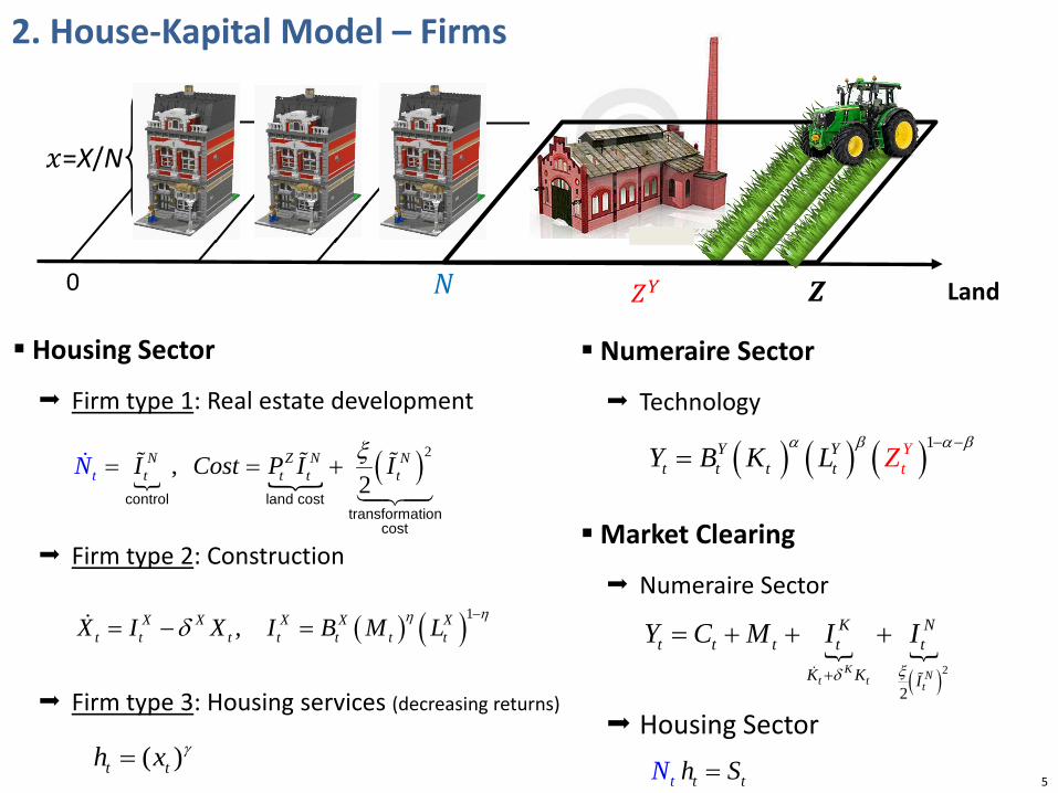
2. House-Kapital Model – Firms

Housing Sector

Firm type 1: Real estate development

Firm type 2: Construction

Firm type 3: Housing services (decreasing returns)

( )2

2, Z N N

t tt tN

t Cost P I IIN ξ= +=

land costtransformation

co

contr l

st

o

( ) ( )1,X X X X Xt t t t t t tX I X I B M L

ηηδ−

= − =

( )t th x γ=tt tN h S=

𝒁𝒁 0 𝑁𝑁

𝑥𝑥=X/N

Land

Numeraire Sector

Technology

Market Clearing

Numeraire Sector

Housing Sector

( ) ( ) ( )1Y Yt t t t

YtY B K L Z

α β α β− −=

( )

2

2 tt t NK

t

I

K Nt t t t

K K

Y C M I Iδ ξ+

+ += +

𝑍𝑍𝑌𝑌


2. House-Kapital Model – Households

Household Optimization

Private Wealth

( )

( )

0 0{ , }

0

max log log

s.t. (1 ) (1 )

lim exp (1 )(0) given 0

t t t

tt t

C S

t r t t w t t t t t t

t

t r stW

C S e dt

W rW w L C p S T

W r ds

ρθ

τ τ

τ

∞=

∞ −

→∞

+

= − + − − −

−=

+

− ≥

∫

∫

: total financial asset holding non-residential land housing wealth non-residential wealth

Ht t

t

P N

N X Z Y H Z Yt t t t t t t t t t t t t

A

W q N q X K P Z P N K P Z≡ + + + = + +


2. House-Kapital Model – Dynamic System

7 dynamic equations…

plus a set of static equations…

( )

( )

( )

11 1

1

(1 )

1

1

X X

YZ Y

K Y

X

w B q

w LR Br Z

R p x

px

ηη η

α βα

γ

γ

η η

αα ββ δ

γ

π γ

− −

+

−

= −

= − − +

=

= −

# housing housing projects services

per firm

Y

X Y

N X Z YW

Xx

Z N Z

L L L

K q N q X P Z

N

N

S xγ

=

+ =

= + + +

=

=

+

11

11

1

YK

X

X X

K YY

Y

C pS

wK Lr

LM q B

r w ZBL

η

α α βα

θ

αβ δ

η

δα β

−

− −−

=

=+

=

+=

( )1X X X

N Z

X B M L X

q PN

ηη δ

ξ

−= −

−=

[ ](1 )r

W rW wL C pS

C C rτ ρ

= + − −

= − −

( )

N N

Z Z Z

X X X X

q rq

P rP R

q r q R

π

δ

−

−

=

= + −

=

Analytical steady states Transitional dynamics


3. Thinking Long Term – Steady States

𝑃𝑃𝑍𝑍∗ and 𝑃𝑃𝐻𝐻∗ depend positively on 𝐵𝐵𝑌𝑌 and 𝐷𝐷 ≔ 𝐿𝐿/𝑍𝑍 (not on 𝐵𝐵𝑋𝑋)

Ricardo's (1817) principle of scarcity.

( ) ( )1 1

* *1 1 1 1( ) ( )Y H YZP a r PD b r DB Bβ β

α α α α∗ ∗− − − −

− −= =

Does not depend on 𝐵𝐵𝑋𝑋, 𝐵𝐵𝑌𝑌 or 𝐷𝐷

Same for other ratios, such as

• non-residential wealth-to-income ratio 𝐾𝐾∗+𝑃𝑃𝑍𝑍∗𝑍𝑍𝑌𝑌∗

𝑁𝑁𝑁𝑁𝑃𝑃∗

• House price-to-rent ratio 𝑃𝑃𝐻𝐻∗

𝑝𝑝∗ℎ∗.

Land price & house price

Housing wealth-to-income ratio 𝑃𝑃𝐻𝐻∗𝐻𝐻∗

𝑁𝑁𝑁𝑁𝑃𝑃∗

Number of houses per unit of land, 𝑁𝑁∗/𝑍𝑍

Does not depend on 𝐵𝐵𝑋𝑋, 𝐵𝐵𝑌𝑌 or 𝐷𝐷 Increases in housing demand do not affect long land allocation

Residential structures per unit of land, 𝑋𝑋∗/𝑍𝑍, are increasing in 𝐵𝐵𝑋𝑋, 𝐵𝐵𝑌𝑌 and 𝐷𝐷


3. Thinking Long Term – Calibration Initial conditions Initial housing stock (𝑁𝑁0, 𝑋𝑋0) set to match empirical 𝑃𝑃0

𝐻𝐻𝑁𝑁0𝑁𝑁𝑁𝑁𝑃𝑃0

in 1955

Initial capital (𝐾𝐾0) set to match empirical 𝐾𝐾0+𝑃𝑃0𝑍𝑍𝑍𝑍0𝑌𝑌

𝑁𝑁𝑁𝑁𝑃𝑃0 in 1955

Growth in TFP (𝐵𝐵𝑡𝑡𝑋𝑋, 𝐵𝐵𝑡𝑡𝑌𝑌) Matches GDP growth between 1955 and 2010 Given observed growth in population size (𝐿𝐿𝑡𝑡)

Directly observable Depreciation rates 𝛿𝛿𝐾𝐾, 𝛿𝛿𝑋𝑋 Capital income tax rate 𝜏𝜏𝑟𝑟

Other observables set to match Expenditure share for housing services Labor income share Value-added of residential construction Sectorial employment shares Sectorial investment rates


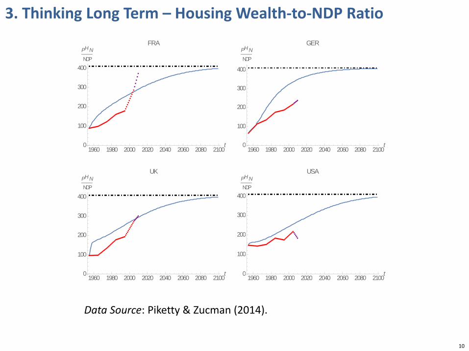
1960 1980 2000 2020 2040 2060 2080 2100t0

100

200

300

400

PHNNDP

FRA

1960 1980 2000 2020 2040 2060 2080 2100t0

100

200

300

400

PHNNDP

GER

1960 1980 2000 2020 2040 2060 2080 2100t0

100

200

300

400

PHNNDP

UK

1960 1980 2000 2020 2040 2060 2080 2100t0

100

200

300

400

PHNNDP

USA

Data Source: Piketty & Zucman (2014).

3. Thinking Long Term – Housing Wealth-to-NDP Ratio


3. Thinking Long Term – House Price & Land Price

Land price (1955 – 2010): Model: factor 7.5; Data: factor 5.2 (France, UK, USA)

House price (1955 – 2010): Model: factor 3.4; Data: factor 3.2 (France, UK, USA)

Calibrated Model

1960 1980 2000 2020 2040 2060 2080 2100

2

4

6

8

10

12

Land price PZ

House price PH


Caselli-Ventura (AER 2000) structure with 𝐽𝐽 groups of HH.

Heterogeneity in initial wealth holding (percentiles, US): 𝑊𝑊𝑗𝑗(0) with 𝑗𝑗 ∈ 1, … , 𝐽𝐽 .

Representative consumer, despite non-homothetic preferences.

If 𝜙𝜙 > 0, poorer HH has higher housing expenditure share

Two-stage numerical solution procedure.

( )

0

11

0{ , }

capital non-residential land houses

:

(

( ) 1max

1

s.t. (1 ) (1

0) given, NPGC holds

)

j j t

j j t

c s

j r j w j j j

Z Y Hj j j j

j

c s se dt

W rW wL c ps T

W K P Z P N

W

σθ θ

ρφ

σ

τ τ

∞=

−−

∞ −

=

− − −

= − + − − − +

= + +

∫

4. Dynamics of Wealth Inequality – Households Grossmann, Larin, Loefflad & Steger (2017)

1 (:

1 )

jj

j j

j

pse

c pss s

θφθ

= =+ − −


4. Dynamics of Wealth Inequality – Results (1)

How does economic growth affect the distribution of wealth?

Experiment / calibration strategy Exogenous TFP growth and endogenous capital accumulation (population constant). State variables such that wealth-to-income ratios (2010) are matched. Portfolio structure of HH equals aggregate portfolio structure. Initial wealth distribution (percentiles) from World Wealth and Income Database.

Amplification of increase in wealth inequality if expenditure shares differ.

Rent increase affects the poor more, suppresses their ability to accumulate wealth.

(percent)


4. Dynamics of Wealth Inequality – Welfare

How does economic growth affect the HH-specific welfare?

EV measure: 𝜓𝜓𝑗𝑗 is factor of the ideal consumption index each period in baseline scenario (0) such that HH j is indifferent to alternative scenario (1).

All prefer the growth scenario Rich prefer it more than the poor Difference more pronounced if

housing expenditure shares differ!


4. Dynamics of Wealth Inequality – Rent Control

Effect of rent control in growing economy on HH-specific welfare: 𝑝𝑝 ≤ 𝑝𝑝𝑚𝑚𝑚𝑚𝑚𝑚

Poor prefer alternative scenario, rich dislike alternative scenario!

If 𝜙𝜙 > 0, representative agent may prefer alternative scenario: No equity-efficiency trade-off


5. Summary & Conclusions

New Housing & Macro Model: Think Long Term Real estate development (extensive margin) withdraws land from alternative uses Investment in structures (intensive margin) does not require land Consistent with evidence that 80 percent of house price increase since WWII is

associated with rising land prices (Knoll et al., 2017) Rising wealth-to-income ratio over time (housing vs. non-residential wealth)

• In long run (for baseline calibration): 𝟒𝟒𝟒𝟒𝟒𝟒 + 𝟑𝟑𝟑𝟑𝟒𝟒 = 𝟕𝟕𝟑𝟑𝟒𝟒 (percent) • Sensitive w.r.t. long run interest rate • But independent of TFP and population size

Wealth inequality and welfare Secular increase in housing demand associated with rising wealth inequality Amplified by endogenous heterogeneity in housing expenditure shares

Poor prefer rent ceiling, while rich dislike rent ceiling

Rent control possibly efficiency-enhancing


Supplement – Wealth-to-NDP ratios: Long Run Implications

𝟒𝟒𝟒𝟒𝟒𝟒 + 𝟑𝟑𝟑𝟑𝟒𝟒 = 𝟕𝟕𝟑𝟑𝟒𝟒


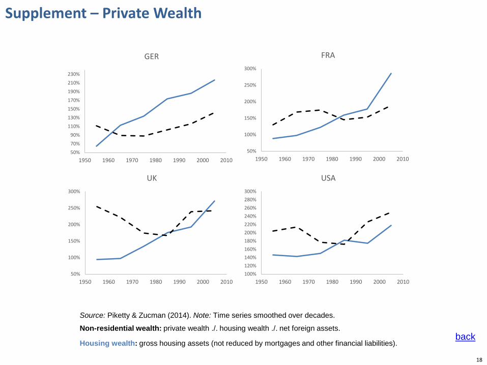
Housing wealth-to-NDP ratio Non-residential wealth-to-NDP ratio

Source: Piketty & Zucman (2014). Note: Time series smoothed over decades.

Non-residential wealth: private wealth ./. housing wealth ./. net foreign assets.

Housing wealth: gross housing assets (not reduced by mortgages and other financial liabilities).

Supplement – Private Wealth

100%120%140%160%180%200%220%240%260%280%300%

1950 1960 1970 1980 1990 2000 2010

USA

50%

70%

90%

110%

130%

150%

170%

190%

210%

230%

1950 1960 1970 1980 1990 2000 2010

GER

50%

100%

150%

200%

250%

300%

1950 1960 1970 1980 1990 2000 2010

FRA

50%

100%

150%

200%

250%

300%

1950 1960 1970 1980 1990 2000 2010

UK

back


Supplement – House Prices & Land Prices

Source: Knoll et al. (2017) back


Source: Knoll et al. (2017)

Supplement – House Prices (country by country)

back


Numeraire good

𝑌𝑌𝑡𝑡 = 𝐵𝐵𝑡𝑡𝑌𝑌 𝐾𝐾𝑡𝑡𝑌𝑌 𝛼𝛼 𝐿𝐿𝑡𝑡𝑌𝑌 1−𝛼𝛼

non-residential land missing

Construction

𝑋𝑋𝑡𝑡 = 𝐵𝐵𝑡𝑡𝑋𝑋 𝐾𝐾𝑡𝑡𝑋𝑋 𝛾𝛾 𝐿𝐿𝑡𝑡𝑋𝑋 1−𝛾𝛾

intermediate input

Housing services

𝐵𝐵𝑡𝑡𝐻𝐻𝑋𝑋𝑡𝑡𝛽𝛽�̅�𝑍1−𝛽𝛽

gross investment

= 𝐻𝐻𝑡𝑡�̇net

investment

+ 𝛿𝛿𝐻𝐻𝐻𝐻𝑡𝑡replacementinvestment

𝒁𝒁� is (time-invariant) flow variable

Housing market clearing

𝑆𝑆𝑡𝑡 = 𝑝𝑝𝑡𝑡 𝐻𝐻𝑡𝑡

housing consumption

Capital market clearing

𝐾𝐾𝑡𝑡𝑋𝑋+𝐾𝐾𝑡𝑡𝑌𝑌 = 𝐾𝐾𝑡𝑡

Labor market clearing

𝐿𝐿𝑡𝑡𝑋𝑋+𝐿𝐿𝑡𝑡𝑌𝑌 = 𝐿𝐿𝑡𝑡

Supplement: Canonical Model

Davis and Heathcote (2005), Hornstein (2009), Iacoviello and Neri (2010), Favilukis et al. (2015), and Borri and Reichlin (2016)

Merits & Features Suitable for business cycle phenomena Limited land scarcity / No land rivalry

Long-run inconsistency: Replacement investment require land: ∫ �̅�𝑍𝑑𝑑𝑡𝑡∞0 = ∞!


Supplement – Comparison of Models Land Price in Response to Housing Stock Destruction

0 20 40 60 80 100 120 140t

1.05

1.10

1.15

1.20

1.25

PZa Canonical Model: H0 0.8H

0 20 40 60 80 100 120 140t

0.950.960.970.980.991.00

PZb House Capital Model: N0 0.8N , X0 0.8X

0 20 40 60 80 100 120 140t

0.990

0.992

0.994

0.996

0.998

1.000PZ

c House Capital Model: N0 0.8N , X0 X

0 20 40 60 80 100 120 140t

0.96

0.97

0.98

0.99

1.00PZ

d House Capital Model: N0 N , X0 0.8X

Two models differ on isolated impact of housing stock destruction on 𝑃𝑃𝑍𝑍 dynamics.

The reason is that the land price determination is different!


A general equilibrium consists of sequences of quantities, prices, and operating profits of housing services producers

for initial conditions (𝐾𝐾0, 𝑁𝑁0, 𝑋𝑋0) > 0 and 𝐵𝐵𝑡𝑡𝑌𝑌 ,𝐵𝐵𝑡𝑡𝑋𝑋 ,𝐵𝐵𝑡𝑡ℎ , 𝐿𝐿𝑡𝑡 𝑡𝑡=0∞ such that

1. representative household maximizes lifetime utility;

2. representative firm in 𝑋𝑋 sector and 𝑌𝑌 sector, representative real estate developer, and housing services producer maximize PDV of infinite profit stream, taking prices as given;

3. land market, labor market, bond market and market for structures clear: 𝑍𝑍𝑡𝑡𝑌𝑌 + 𝑁𝑁𝑡𝑡 = 𝑍𝑍, 𝐿𝐿𝑡𝑡𝑋𝑋 + 𝐿𝐿𝑡𝑡𝑌𝑌 = 𝐿𝐿𝑡𝑡, 𝐾𝐾𝑡𝑡𝑌𝑌 = 𝐾𝐾𝑡𝑡, 𝑋𝑋𝑡𝑡 = 𝑁𝑁𝑡𝑡𝑥𝑥𝑡𝑡;

4. land price is the PDV of rental rates per unit of land in 𝑌𝑌 sector;

5. financial asset market clears: 𝐾𝐾𝑡𝑡 + 𝑞𝑞𝑡𝑡𝑁𝑁𝑁𝑁𝑡𝑡 + 𝑞𝑞𝑡𝑡𝑋𝑋𝑋𝑋𝑡𝑡 + 𝑃𝑃𝑡𝑡𝑍𝑍𝑍𝑍𝑡𝑡𝑌𝑌 = 𝑊𝑊𝑡𝑡;

6. market for housing services clears: 𝑆𝑆𝑡𝑡 = 𝑁𝑁𝑡𝑡ℎ𝑡𝑡;

7. market for Y good clears: 𝑌𝑌𝑡𝑡 = 𝐶𝐶𝑡𝑡 + 𝐼𝐼𝑡𝑡𝐾𝐾 + 𝐼𝐼𝑡𝑡𝑁𝑁 + 𝑀𝑀𝑡𝑡 (redundant due to Walras’ law)

Supplement: General Equilibrium

This image cannot currently be displayed.


Symbol Meaning Y final output of numeraire good

KY=K physical capital

LX, LY labor in 𝑋𝑋 and 𝑌𝑌 production

ZY land in 𝑌𝑌 sector

X, x=X/N residential buildings (aggregate and per house)

M materials (in terms of numeraire)

δK, δX depreciation rates (physical capital and buildings)

N number of housing projects

qN, , qX shadow price of N and X

RZ, PZ rental rate and price of land

h housing services (per housing project)

S=Nh total housing services‘ demand and supply

τr , τw , T policy parameters

Supplement – Notation

Das House-Kapital: A Long Term Housing & Macro … House-Kapital: A Long Term Housing & Macro Model....

Documents

Transcript of Das House-Kapital: A Long Term Housing & Macro … House-Kapital: A Long Term Housing & Macro Model....