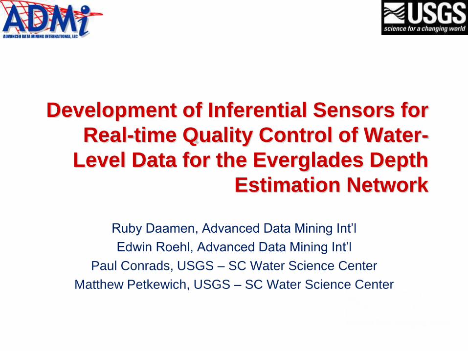
Development of Inferential Sensors for

Real-time Quality Control of Water-

Level Data for the Everglades Depth

Estimation Network

Ruby Daamen, Advanced Data Mining Int’l

Edwin Roehl, Advanced Data Mining Int’l

Paul Conrads, USGS – SC Water Science Center

Matthew Petkewich, USGS – SC Water Science Center

Presentation Outline

• What is an “Inferential Sensor” (IS)?

• Background - Industrial application

• Everglades Depth Estimation Network

(EDEN)

• Automated Data Assurance and

Management (ADAM) - Inferential Sensor

development for EDEN

Development of IS in Industry

• A tough environment to monitor

– Emissions regulations require measurements of

effluent gases

– Smoke stack burns up probes

– Need alternative to “hard” sensors

Hard Sensor vs. Inferential Sensor

• Virtual sensor replaces actual sensor

– Temporary gage smoke stack

– Operate plant to cover range of emissions

– Develop model of emissions based on

operations

– Model becomes the “Inferential Sensor”

Inferential Sensors for Real-Time Data

• Problem – Need to minimize missing and

erroneous data

• Use similar approach taken by industry to predict

real-time data – ie. “Inferential Sensors”

– QA/QC hard sensor

– Provide accurate estimates for hard sensor

– Provide redundant signal

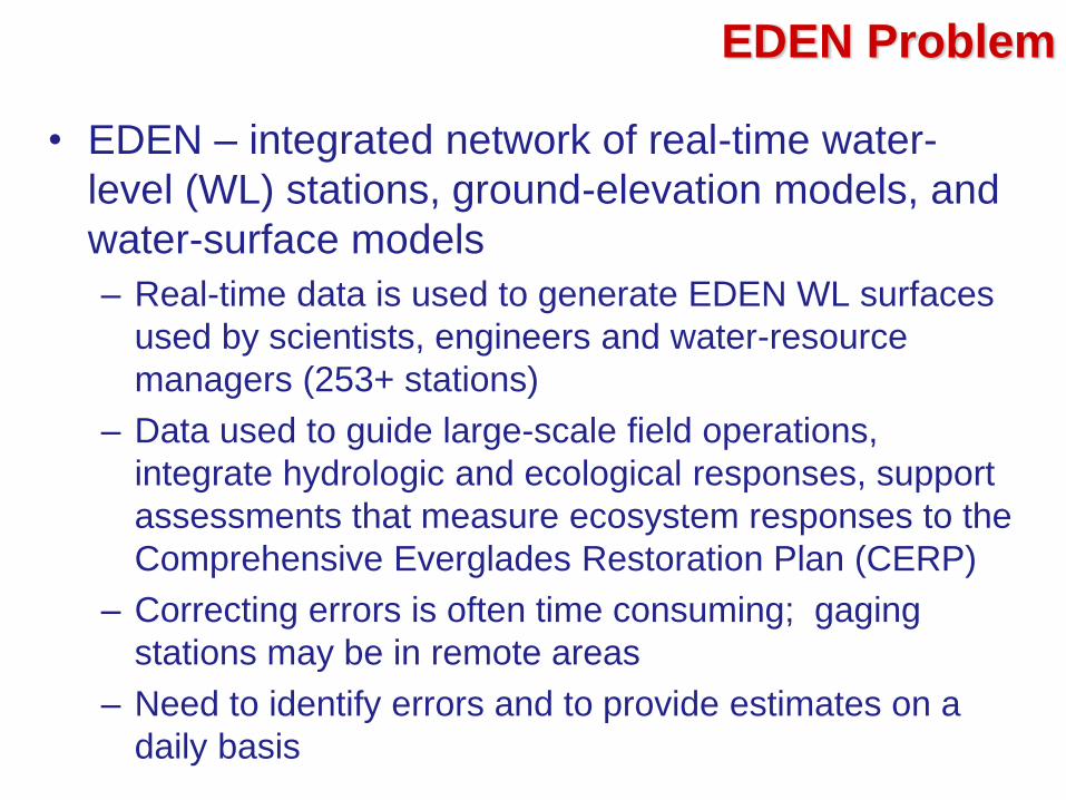
EDEN Problem

• EDEN – integrated network of real-time water-

level (WL) stations, ground-elevation models, and

water-surface models

– Real-time data is used to generate EDEN WL surfaces

used by scientists, engineers and water-resource

managers (253+ stations)

– Data used to guide large-scale field operations,

integrate hydrologic and ecological responses, support

assessments that measure ecosystem responses to the

Comprehensive Everglades Restoration Plan (CERP)

– Correcting errors is often time consuming; gaging

stations may be in remote areas

– Need to identify errors and to provide estimates on a

daily basis

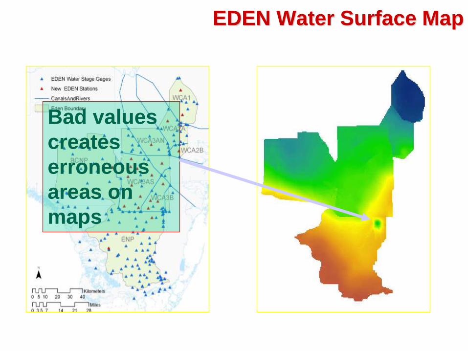
EDEN Water Surface Map

Bad values

creates

erroneous

areas on

maps

EDEN / ADAM Overview

Inferential Sensor

application

Some of the Challenges

• 253+ gaging stations

• Inferential sensor uses data from one or

more correlated gages. At any given

datetime do not know what stations will have

available data

• Stations added/removed over time

Implementation

• Create models “on the fly”

– Use “best” available stations

– Simplifies addition / removal of stations

• Needs to consider

– Assessment of data – prevent use of suspect

data in models

– Model inputs need be decorrelated

Methods

• Two algorithms sequenced to analyze data

– Univariate filtering

• Provides information about the quality and behavior

for each stations WL

• A Statistical Process Control (SPC) which consists of

14 univariate filters – uniquely set for each station

– Estimate parameter value

• Select a “pool” of candidate gaging stations using

matrix of Pearson coefficients

• Principal component analysis (PCA) – calculates

decorrelated inputs

• Multivariate linear regression

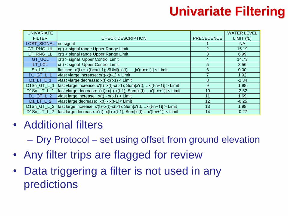
Univariate Filtering

UNIVARIATE

FILTER CHECK DESCRIPTION PRECEDENCE

WATER LEVEL

LIMIT (ft.)

LOST_SIGNAL no signal 1 NA

GT_RNG_UL x(t) > signal range Upper Range Limit 2 15.19

LT_RNG_LL x(t) < signal range Upper Range Limit 3 6.99

GT_UCL x(t) > signal Upper Control Limit 4 14.73

LT_LCL x(t) < signal Upper Control Limit 5 8.56

Sn_LT_L flatlined: x'(t) = x(t)=x(t-1); SUM[(|x'(t)|,…,|x'(t-n+1)|] < Limit 6 0.00

D1_GT_L_1 vfast vlarge increase: x(t)-x(t-1) > Limit 7 1.92

D1_LT_L_1 vfast vlarge decrease: x(t)-x(t-1) < Limit 8 -2.34

D1Sn_GT_L_1 fast vlarge increase: x'(t)=x(t)-x(t-1); Sum[x'(t),…x'(t-n+1)] > Limit 9 1.98

D1Sn_LT_L_1 fast vlarge decrease: x'(t)=x(t)-x(t-1); Sum[x'(t),…x'(t-n+1)] < Limit 10 -2.52

D1_GT_L_2 vfast large increase: x(t) - x(t-1) > Limit 11 1.69

D1_LT_L_2 vfast large decrease: x(t) - x(t-1)< Limit 12 -0.25

D1Sn_GT_L_2 fast large increase: x'(t)=x(t)-x(t-1); Sum[x'(t),…x'(t-n+1)] > Limit 13 1.98

D1Sn_LT_L_2 fast large decrease: x'(t)=x(t)-x(t-1); Sum[x'(t),…x'(t-n+1)] < Limit 14 -0.27

• Additional filters

– Dry Protocol – set using offset from ground elevation

• Any filter trips are flagged for review

• Data triggering a filter is not used in any

predictions

Synthesize WL Measurements

• WL at candidate stations are correlated – no

surprise

• First approach examined selected the most

highly correlated station as a “standard”

signal and then attempted decorrelating the

other stations by computing differences from

the standard.

Principal Component Analysis (PCA)

• PCA is a statistical technique used to

“reduce the dimensionality of a data set

consisting of a large number of interrelated

variables, while retaining as much as

possible of the variation present in the data

set. This is achieved by transforming to a

new set of variables, the principal

components (PCs), which are uncorrelated,

and which are ordered so that the first few

retain most of the variation present in all of

the original variables” (Joliffe)

PCA – Main Points

• PCA - the main points

– Principal components are uncorrelated

– Transforms a set of correlated variables into a

smaller number of uncorrelated variables

– The first principal component (PC) accounts for

most of the variability in the data

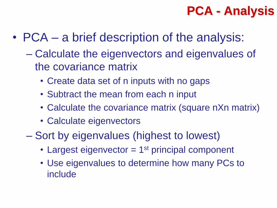
PCA - Analysis

• PCA – a brief description of the analysis:

– Calculate the eigenvectors and eigenvalues of

the covariance matrix

• Create data set of n inputs with no gaps

• Subtract the mean from each n input

• Calculate the covariance matrix (square nXn matrix)

• Calculate eigenvectors

– Sort by eigenvalues (highest to lowest)

• Largest eigenvector = 1st principal component

• Use eigenvalues to determine how many PCs to

include

PCA – A 2-Dimension ExampleOriginal Data

(Mean Subtracted)

Eigenvectors Principal

Components

Eigenvectors

Plotted on

Data

-4

-3

-2

-1

0

1

2

3

4

-4 -3 -2 -1 0 1 2 3 4

Normalized Data

E1

E2

Original Data

ADAM - Functionality

• Setup

– File paths

– PCA setup – period, number of sites to include

– Add / Edit / Remove sites

– Univariate filters

• Inferential Sensor – Option to analyze daily

(hourly and 15 minute data), quarterly and

annual (hourly) daily files

• Review results

• Output daily median files as required for

EDEN water surface map

ADAM – Control Worksheet

Select Daily, Quarterly or

Annual Run Analysis

Resume, redo OR continue from

last analyzed

Fill Setup

Remove , add, or edit sites

included in ADAM

Set Pathnames for files used

by ADAM

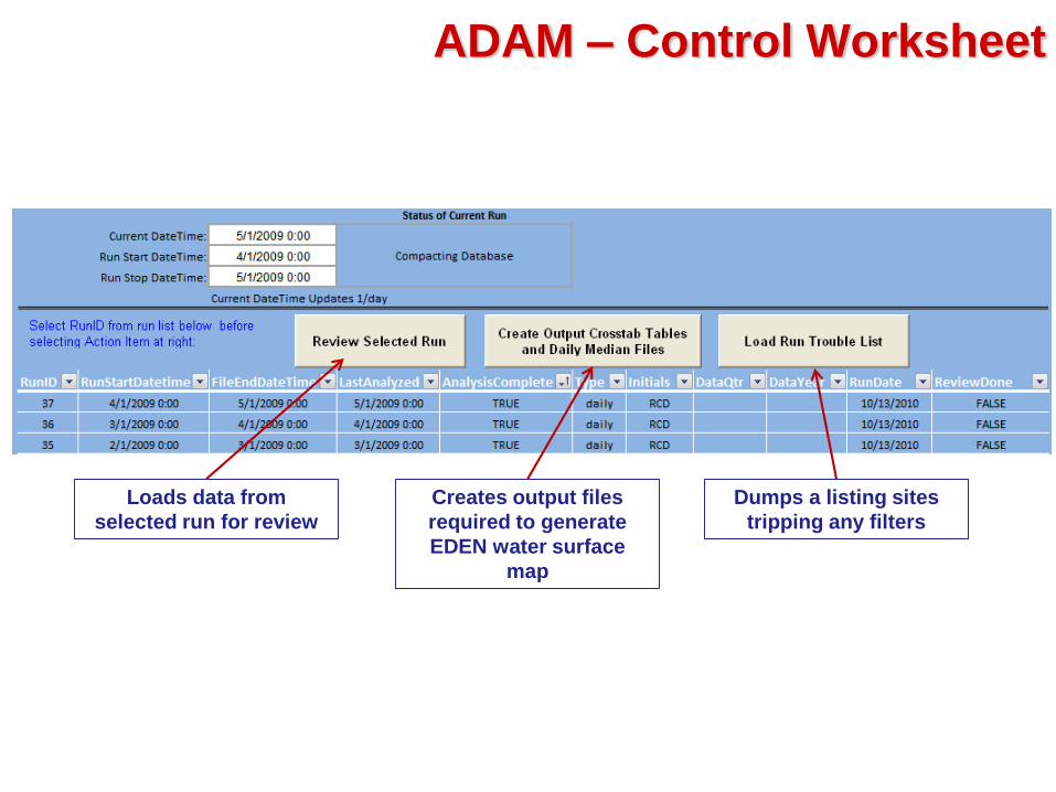
ADAM – Control Worksheet

Loads data from

selected run for review

Creates output files

required to generate

EDEN water surface

map

Dumps a listing sites

tripping any filters

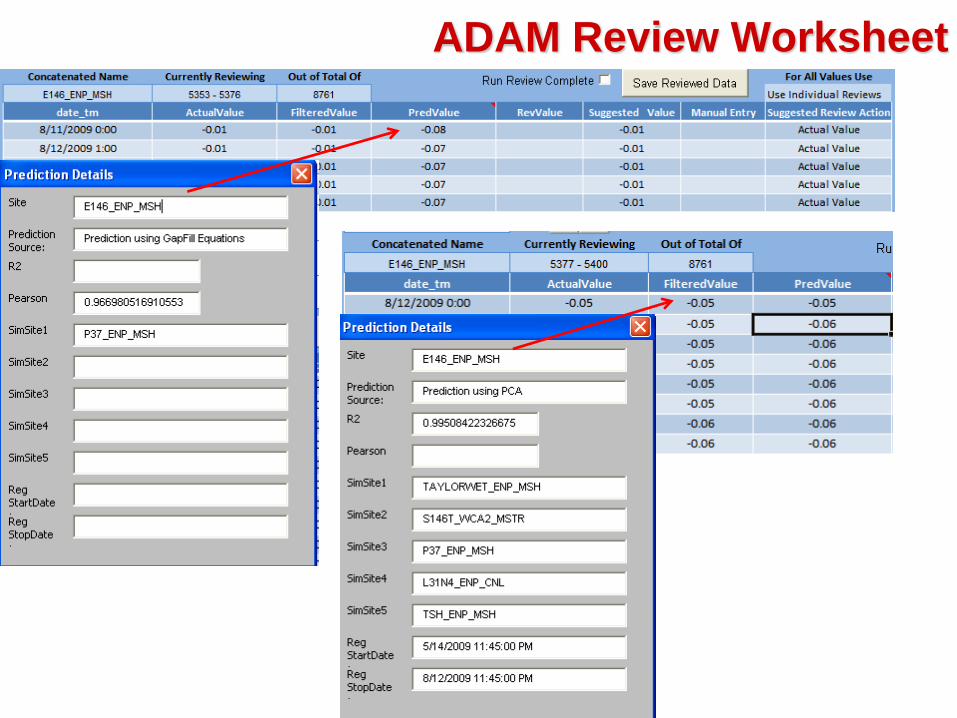
ADAM Review Worksheet

First PCA

analysis

GAPFILL

ADAM Review Worksheet

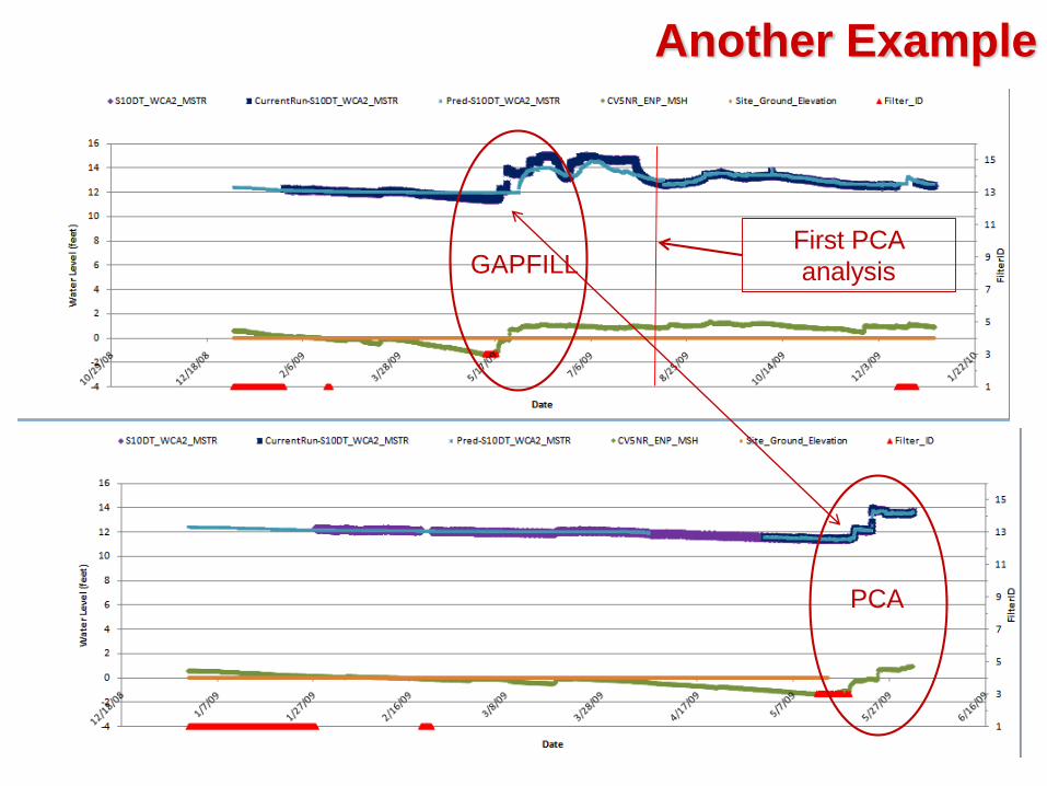
Another Example

GAPFILL

PCA

First PCA

analysis

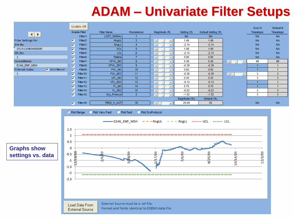
ADAM – Univariate Filter Setups

Graphs show

settings vs. data

What’s Next

EVEEvolution and Verification of EDEN Inferential Sensor

Questions?

Archive

PCA – The methodology

• From our favorite source -Wikipedia – PCA is:– A mathematical procedure that transforms a set of correlated variables into a smaller number of

uncorrelated variables. The first principal component accounts for as much of the variability in the data as possible and each succeeding component accounts for as much of the remaining variability as possible.

• How to do it: In the broadest sense it is an eigenvector based multivariate analysis. The methodology used is:

– Assemble the data• In EDENIS the data will be water level data from up to 5 gaging stations. For 90 days of hourly data this

equates to up to 2160 vectors (8640 for 15 minute data)

– Remove any vectors that contain any missing data (1)• Resulting matrix X[n,m] where n = number of fully populated vectors; m = number of gages included

– Subtract the mean from each of the data dimensions (m) – lets call this the normalized matrix B (2)

• B[n,m] stores mean-subtracted data

– Calculate the Covariance matrix (3)• Covariance matrix is a square matrix with dimension mXm: C[m,m]

– Calculate the eigenvalues and eigenvectors of the covariance matrix• This is an iterative process. If you want to look up some more on this I used the Jacobi eigenvalue

algorithm. Some important properties of eigenvectors:– Can only be found for square matrices. If a square matrix (mXm) does have eigenvectors, there are m of them– All the eigenvectors of a matrix are orthogonal to each other. This is important: when the data is expressed in terms of

these eigenvectors the resulting principal components are uncorrelated

• For a refresher course on eigenvalues / eigenvectors heres a link http://en.wikipedia.org/wiki/Eigenvalue,_eigenvector_and_eigenspace

– Sort the results: Largest eigenvalue to smallest eigenvalue. (4)– Decide how many components to keep and calculate the new data set to be used. This is a

simple matrix multiplication of B X E where E is the mXm eigenvector matrix. (5) • For the 10-12 sites I looked at when presenting the PCA results I would expect we’ll rarely if ever use more

than 2 principal components out of a possible 5 to make the regression predictions.

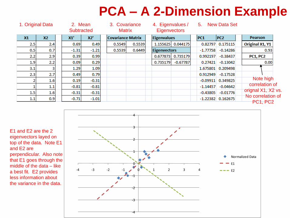
PCA – A 2-Dimension Example1. Original Data 2. Mean

Subtracted

3. Covariance

Matrix

4. Eigenvalues /

Eigenvectors

5. New Data Set

Note high

correlation of

orignal X1, X2 vs.

No correlation of

PC1, PC2

E1 and E2 are the 2

eigenvectors layed on

top of the data. Note E1

and E2 are

perpendicular. Also note

that E1 goes through the

middle of the data – like

a best fit. E2 provides

less information about

the variance in the data.

-4

-3

-2

-1

0

1

2

3

4

-4 -3 -2 -1 0 1 2 3 4

Normalized Data

E1

E2

Challenges

• Develop 253+ models using artificial neural

networks (ANNs) (1 model per station)

– Pros

• authors have prior success modeling complex

processes using ANNs

• ANNs use non-linear curve fitting to capture complex

behaviors

– Cons

• Do not know what stations will have “good” data at

any given datetime

• Stations are removed and added

• Possibly insert Yearly run – min/max r2

using pca,gapfill