Vol. 43 (2012) ACTA PHYSICA POLONICA B No 10

CROSS-CORRELATIONS BETWEEN WTI CRUDEOIL MARKET AND U.S. STOCK MARKET:A PERSPECTIVE FROM ECONOPHYSICS

Gang-Jin Wang, Chi Xie†

College of Business Administration, Hunan UniversityNo. 11 Lushan South Road, Changsha 410082, China

(Received July 27, 2012; revised version received August 23, 2012)

In this study, we take a fresh look at the cross-correlations betweenWTI crude oil market and U.S. stock market from the perspective ofeconophysics. We choose the three major U.S. stock indices (i.e., DJIA,NASDAQ and S&P 500) as the research objects and select the sample datafrom Jan 2, 2002 to Jun 29, 2012. In the empirical process, first, usinga statistical test in analogy to the Ljung-Box test, we find that there arecross-correlations between WTI and DJIA, WTI and NASDAQ, and WTIand S&P 500 at the 5% significance level. Then, employing the multifractaldetrended cross-correlation analysis (MF-DCCA) method, we find that thecross-correlated behavior between WTI crude oil market and U.S. stockmarket is nonlinear and multifractal. An interesting finding is that thecross-correlation exponent is smaller than the average scaling exponentwhen q<0, and larger than the average scaling exponent when q>0. Fi-nally, using the rolling windows method, which can capture the dynamicsof cross-correlations, we find that there are three special periods whosetime-varying Hurst exponents are different from the others.

DOI:10.5506/APhysPolB.43.2021PACS numbers: 89.65.Gh, 89.75–k, 05.45.Df, 05.40.–a

1. Introduction

Financial markets are considered as complex dynamic systems [1, 2].One of the important features of market dynamics is the presence of cross-correlations between financial variables [3]. Although the price changes ofthe crude oil market are usually acknowledged as an important incentivefor the price fluctuations of the stock market, the economists do not reacha consensus on the cross-correlations between crude oil prices and stockprices [4]. For instance, Jones and Kaul [5] first revealed a stable negative

† xiechi@hnu.edu.cn

(2021)

2022 Gang-Jin Wang, Chi Xie

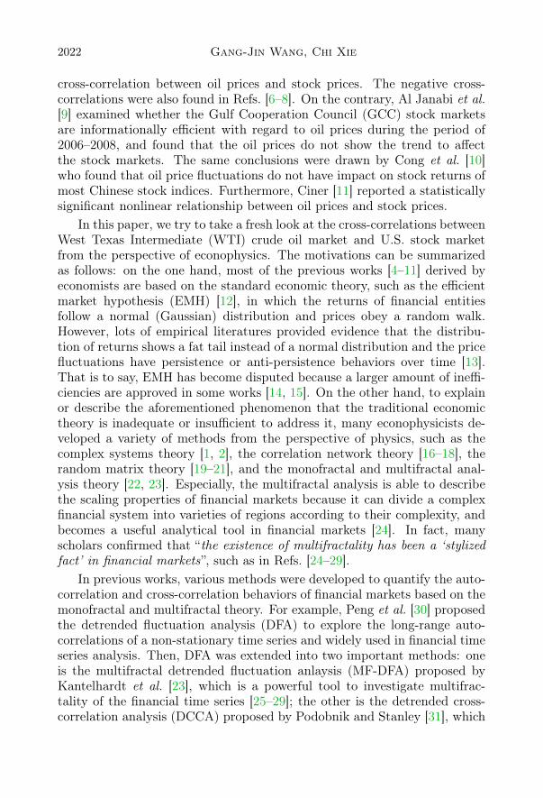
cross-correlation between oil prices and stock prices. The negative cross-correlations were also found in Refs. [6–8]. On the contrary, Al Janabi et al.[9] examined whether the Gulf Cooperation Council (GCC) stock marketsare informationally efficient with regard to oil prices during the period of2006–2008, and found that the oil prices do not show the trend to affectthe stock markets. The same conclusions were drawn by Cong et al. [10]who found that oil price fluctuations do not have impact on stock returns ofmost Chinese stock indices. Furthermore, Ciner [11] reported a statisticallysignificant nonlinear relationship between oil prices and stock prices.

In this paper, we try to take a fresh look at the cross-correlations betweenWest Texas Intermediate (WTI) crude oil market and U.S. stock marketfrom the perspective of econophysics. The motivations can be summarizedas follows: on the one hand, most of the previous works [4–11] derived byeconomists are based on the standard economic theory, such as the efficientmarket hypothesis (EMH) [12], in which the returns of financial entitiesfollow a normal (Gaussian) distribution and prices obey a random walk.However, lots of empirical literatures provided evidence that the distribu-tion of returns shows a fat tail instead of a normal distribution and the pricefluctuations have persistence or anti-persistence behaviors over time [13].That is to say, EMH has become disputed because a larger amount of ineffi-ciencies are approved in some works [14, 15]. On the other hand, to explainor describe the aforementioned phenomenon that the traditional economictheory is inadequate or insufficient to address it, many econophysicists de-veloped a variety of methods from the perspective of physics, such as thecomplex systems theory [1, 2], the correlation network theory [16–18], therandom matrix theory [19–21], and the monofractal and multifractal anal-ysis theory [22, 23]. Especially, the multifractal analysis is able to describethe scaling properties of financial markets because it can divide a complexfinancial system into varieties of regions according to their complexity, andbecomes a useful analytical tool in financial markets [24]. In fact, manyscholars confirmed that “the existence of multifractality has been a ‘stylizedfact’ in financial markets”, such as in Refs. [24–29].

In previous works, various methods were developed to quantify the auto-correlation and cross-correlation behaviors of financial markets based on themonofractal and multifractal theory. For example, Peng et al. [30] proposedthe detrended fluctuation analysis (DFA) to explore the long-range auto-correlations of a non-stationary time series and widely used in financial timeseries analysis. Then, DFA was extended into two important methods: oneis the multifractal detrended fluctuation anlaysis (MF-DFA) proposed byKantelhardt et al. [23], which is a powerful tool to investigate multifrac-tality of the financial time series [25–29]; the other is the detrended cross-correlation analysis (DCCA) proposed by Podobnik and Stanley [31], which

Cross-correlations Between WTI Crude Oil Market and U.S. Stock Market . . . 2023

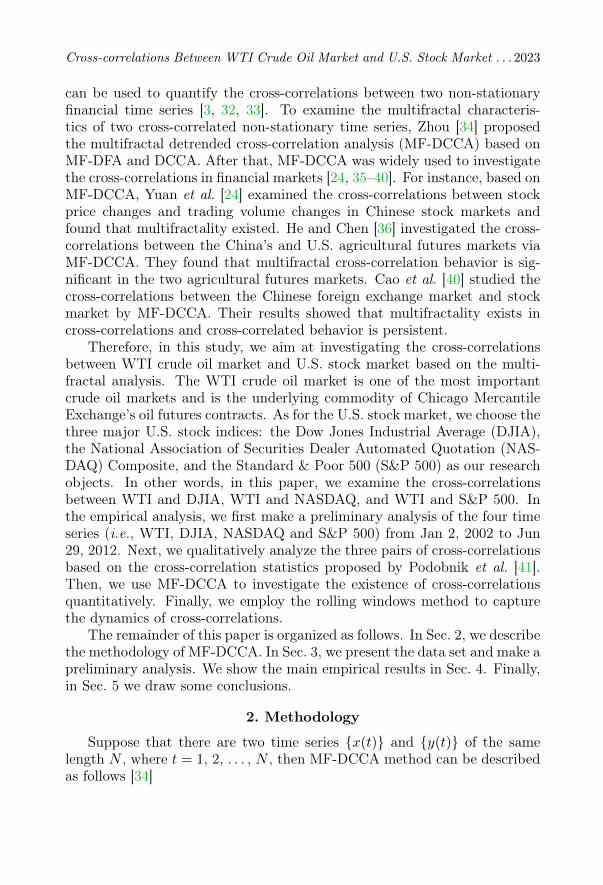
can be used to quantify the cross-correlations between two non-stationaryfinancial time series [3, 32, 33]. To examine the multifractal characteris-tics of two cross-correlated non-stationary time series, Zhou [34] proposedthe multifractal detrended cross-correlation analysis (MF-DCCA) based onMF-DFA and DCCA. After that, MF-DCCA was widely used to investigatethe cross-correlations in financial markets [24, 35–40]. For instance, based onMF-DCCA, Yuan et al. [24] examined the cross-correlations between stockprice changes and trading volume changes in Chinese stock markets andfound that multifractality existed. He and Chen [36] investigated the cross-correlations between the China’s and U.S. agricultural futures markets viaMF-DCCA. They found that multifractal cross-correlation behavior is sig-nificant in the two agricultural futures markets. Cao et al. [40] studied thecross-correlations between the Chinese foreign exchange market and stockmarket by MF-DCCA. Their results showed that multifractality exists incross-correlations and cross-correlated behavior is persistent.

Therefore, in this study, we aim at investigating the cross-correlationsbetween WTI crude oil market and U.S. stock market based on the multi-fractal analysis. The WTI crude oil market is one of the most importantcrude oil markets and is the underlying commodity of Chicago MercantileExchange’s oil futures contracts. As for the U.S. stock market, we choose thethree major U.S. stock indices: the Dow Jones Industrial Average (DJIA),the National Association of Securities Dealer Automated Quotation (NAS-DAQ) Composite, and the Standard & Poor 500 (S&P 500) as our researchobjects. In other words, in this paper, we examine the cross-correlationsbetween WTI and DJIA, WTI and NASDAQ, and WTI and S&P 500. Inthe empirical analysis, we first make a preliminary analysis of the four timeseries (i.e., WTI, DJIA, NASDAQ and S&P 500) from Jan 2, 2002 to Jun29, 2012. Next, we qualitatively analyze the three pairs of cross-correlationsbased on the cross-correlation statistics proposed by Podobnik et al. [41].Then, we use MF-DCCA to investigate the existence of cross-correlationsquantitatively. Finally, we employ the rolling windows method to capturethe dynamics of cross-correlations.

The remainder of this paper is organized as follows. In Sec. 2, we describethe methodology of MF-DCCA. In Sec. 3, we present the data set and make apreliminary analysis. We show the main empirical results in Sec. 4. Finally,in Sec. 5 we draw some conclusions.

2. Methodology

Suppose that there are two time series {x(t)} and {y(t)} of the samelength N , where t = 1, 2, . . . , N , then MF-DCCA method can be describedas follows [34]

2024 Gang-Jin Wang, Chi Xie

Step 1. Determine the “profile” as two new series

X(t) =t∑i=1

(x(i)− 〈x〉) , Y (t) =t∑i=1

(y(i)− 〈y〉) , t = 1, 2, . . . , N . (1)

Step 2. Both of the profiles {X(t)} and {Y (t)} are divided into Ns =int(N/s) non-overlapping segments of equal length s. Since N is often not amultiple of s, a short part at the end of profile may remain. To include thispart of the series, we repeat the same procedure starting from the oppositeend. Therefore, we obtain 2Ns segments. In this study, we set 10 ≤ s ≤ N/5.

Step 3. We estimate the local trends for each of the 2Ns segments by aleast-square fit of each series. Then determine the variance [36, 40]

F 2v (s) =

1

s

s∑t=1

∣∣∣X(v−1)s+t(t)− Xv(t)∣∣∣ ∣∣∣Y(v−1)s+t(t)− Yv(t)∣∣∣ (2)

for each segment v, v = 1, 2, . . . , Ns and

F 2v (s) =

1

s

s∑t=1

∣∣∣XN−(v−Ns)s+t(t)− Xv(t)∣∣∣ ∣∣∣YN−(v−Ns)s+t(t)− Yv(t)

∣∣∣ (3)

for v = Ns + 1, Ns + 2, . . . ,2Ns. Here, Xv(t) and Yv(t) are the fittingpolynomials in segments v, respectively.

Step 4. We average over all segments to obtain the qth order cross-correlation fluctuation function

Fq(s) =

{1

2Ns

2Ns∑v=1

[F 2v (s)

]q/2}1/q

(4)

for any q 6= 0 and

F0(s) =

{1

4Ns

2Ns∑v=1

ln[F 2v (s)

]}. (5)

Step 5. By observing the log–log plots Fq(s) versus s for each value of q,we can determine the scaling behavior of the fluctuation function. If theoriginal series {x(t)} and {y(t)} are power-law cross-correlated, then

Fq(s) ∝ shxy(q) , (6)

where the cross-correlation scaling exponent hxy(q) can be obtained by theslope of log–log plot of Fq(s) versus s via ordinary least squares (OLS) [39].

Cross-correlations Between WTI Crude Oil Market and U.S. Stock Market . . . 2025

Especially, if the time series {x(t)} is identical to {y(t)}, MF-DCCA is equiv-alent to MF-DFA; and when q = 2, MF-DCCA is just DCCA. hxy(q) isalso known as a generalization of Hurst exponent H with the equivalenceH ≡ hxy(2) [42]. If hxy(q) = H for all q, i.e., hxy(q) is independent on q,then the cross-correlations between two time series are monofractal; other-wise they are multifractal.

Generally, there are three cases of hxy(q): (i) If hxy(q) < 0.5, the cross-correlations between the two time series are anti-persistent (negative). Thisimplies that one price is likely to increase following a decrease of the otherprice, and vice versa [35]. (ii) If hxy(q) > 0.5, the cross-correlations betweenthe two time series are persistent (positive). This means that an increase(a decrease) of one price is likely to be followed by an increase (a decrease)of the other price [35]. (iii) If hxy(q) = 0.5, there are no cross-correlationsbetween the two time series, and the change of one price cannot affect thebehavior of the other price [35].

By analyzing the spectrum of the cross-correlations scaling exponenthxy(q), we can calculate the singularity strength α and the multifractalspectrum f(α) by [42]

α = hxy(q) + qh′xy(q) (7)

andf(α) = q[α− hxy(q)] + 1 , (8)

where h′xy(q) stands for the derivative of hxy(q) with respect to q. In this

study, we set q ranging from −10 to 10 with a step of one.The strength of multifractality can be defined by the width of the mul-

tifractal spectrum [36], which is presented as follows

∆α = αmax − αmin . (9)

3. Date and preliminary analysis

We choose the daily closing prices of WTI, DJIA, NASDAQ andS&P 500 from Jan 2, 2002 to Jun 29, 2012. The WTI crude oil spot pricesare provided by U.S. Energy Information Administration (EIA)(http://www.eia.gov/petroleum). We obtain the daily closing prices ofthe three major U.S. stock indices (i.e., DJIA, NASDAQ and S&P 500)from Yahoo Finance (http://finance.yahoo.com).

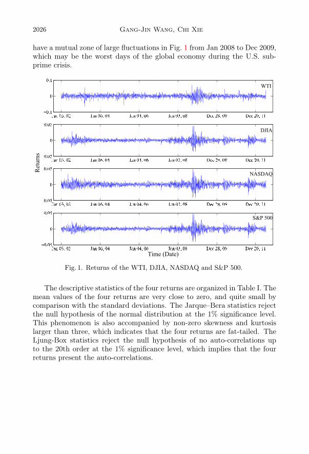
Let P (t) denote the daily closing price on day t. The daily return, r(t),is defined as the logarithmic difference of P (t) and P (t−1), i.e., r(t) =ln(P (t)) − ln(P (t − 1)). The volatility is defined by the absolute return|r(t)|. Figure 1 shows the graphical representation of the four returns (i.e.,WTI, DJIA, NASDAQ and S&P 500). We can find that the four returns

2026 Gang-Jin Wang, Chi Xie

have a mutual zone of large fluctuations in Fig. 1 from Jan 2008 to Dec 2009,which may be the worst days of the global economy during the U.S. sub-prime crisis.

Fig. 1. Returns of the WTI, DJIA, NASDAQ and S&P 500.

The descriptive statistics of the four returns are organized in Table I. Themean values of the four returns are very close to zero, and quite small bycomparison with the standard deviations. The Jarque–Bera statistics rejectthe null hypothesis of the normal distribution at the 1% significance level.This phenomenon is also accompanied by non-zero skewness and kurtosislarger than three, which indicates that the four returns are fat-tailed. TheLjung-Box statistics reject the null hypothesis of no auto-correlations upto the 20th order at the 1% significance level, which implies that the fourreturns present the auto-correlations.

Cross-correlations Between WTI Crude Oil Market and U.S. Stock Market . . . 2027

TABLE I

Descriptive statistics of returns of WTI, DJIA, NASDAQ and S&P 500.

WTI DJIA NASDAQ S&P 500

Mean (×10−4) 2.2430 0.3522 0.5788 0.2228Maximum 0.0713 0.0456 0.0485 0.0476Minimum −0.0660 −0.0356 −0.0416 −0.0411Standard deviation 0.0109 0.0055 0.0067 0.0059Skewness −0.0932 0.0360 −0.0707 −0.1935Kurtosis 7.4528 11.1173 7.5445 11.2824Jarque–Bera (×103) 2.1727∗∗∗ 7.2116∗∗∗ 2.2614∗∗∗ 7.5237∗∗∗Q(20) 65.4455∗∗∗ 97.6337∗∗∗ 57.2772∗∗∗ 98.1227∗∗∗Observations 2623 2623 2623 2623

Notes: The Jarque–Bera statistic tests for the null hypothesis of normality distribution.Q(20) denotes the value of the Ljung-Box statistics of the return series for up to the20th order serial correlation. *** Indicates rejection of the null hypothesis at the 1%significance level.

In order to further examine the fat-tailed distribution of the four returns,we use a novel method of power-law estimation proposed by Podobnik et al.[43]. They indicated that, on average, there is one volatility above thresholdq after each time interval τave(q), then

1/τave(q) ≈∞∫q

P (|x|)d|x| = P (|x| > q) ∼ q−β . (10)

We calculate the average time interval τave(q) for different values of q,and acquire the estimates for β by the relationship

τave(q) ∝ qβ . (11)

The log–log plots of τave(q) versus threshold q are presented in Fig. 2.The thresholds q range from 2σ to 8σ with a fixed step of 0.25σ, where σis the standard deviation of each absolute return. There is a power-lawrelationship with Podobnik’s tail exponent β = 3.2302, β = 3.0233, β =3.4019 and β = 3.0293 for WTI, DJIA, NASDAQ and S&P 500, respectively.One can find that the four Podobnik’s tail exponents are close to three,which is consistent with the “inverse cubic power-law” and is found in manyfinancial markets [28, 37, 43].

2028 Gang-Jin Wang, Chi Xie

Fig. 2. Log–log plots of the average time interval τave(q) versus threshold q

(in units of σ).

4. Empirical results

4.1. Cross-correlation test

In this subsection, we employ a new cross-correlation test proposed byPodobnik et al. [41] to quantify the cross-correlations between WTI crudeoil market and U.S. stock market (i.e., the three pairs of cross-correlations:WTI and DJIA, WTI and NASDAQ, and WTI and S&P 500). This testis analogous to the Ljung-Box test [44] and widely used to test the cross-correlations in the financial markets [24, 35, 37–40]. The cross-correlationstatistic between two time series {x(t)|t = 1, 2, . . . , N} and {y(t)|t = 1, 2,. . . ,N} is defined as

Qcc(m) = N2m∑t=1

C2(t)

N − t, (12)

where the cross-correlation coefficient C(t) is defined by

C(t) =

N∑k=t+1

x(k)y(k − t)√N∑k=1

x2(k)N∑k=1

y2(k)

. (13)

Cross-correlations Between WTI Crude Oil Market and U.S. Stock Market . . . 2029

Podobnik et al. [41] proposed that, the cross-correlation statistic Qcc(m)is approximately χ2(m) distributed with m degrees of freedom. It can beused to test the null hypothesis that none of the first m cross-correlationcoefficients is different from zero [41].

We show the log–log plots of cross-correlation statistics Qcc(m) versusdegrees of freedomm for WTI and DJIA, WTI and NASDAQ, and WTI andS&P 500 in Fig. 3. The degrees of freedom, m, range from 100 to 103. Asa comparison, we also present the critical value for the χ2(m) distributionat the 5% significance level in Fig. 3. For a broad range of m, all the teststatistics Qcc(m) > χ2

0.95(m). Therefore, we can reject the null hypothesisof no cross-correlations. That is to say, cross-correlations evidently existbetween WTI and DJIA, WTI and NASDAQ, and WTI and S&P 500.

100

101

102

103

100

101

102

103

104

m

Qcc(m

)

Test statistics (WTI and DJIA)

Test statistics (WTI and NASDAQ)

Test statistics (WTI and S&P 500)

Critical values

Fig. 3. Log–log plots of test statistics Qcc(m) versus degrees of freedom m.

4.2. Multifractal detrended cross-correlation analysis

Podobnik et al. [41] also proposed that the cross-correlation test basedon the statistic Qcc(m) of Eq. (12) can only test the existence of cross-correlation qualitatively. Thus, in this subsection, we use MF-DCCA ap-proach to investigate the cross-correlation quantitatively by estimating thecross-correlation scaling exponent.

In Figs. 4, 5 and 6, we display the relationship between cross-correlationscaling exponent hxy(q) and q (the curves with circle symbols) for WTI andDJIA, WTI and NASDAQ, and WTI and S&P 500, respectively. Here, wedenote the WTI returns as the {x(t)} time series, and respectively denotethe three returns of DJIA, NASDAQ and S&P 500 as the {y(t)} time series.

2030 Gang-Jin Wang, Chi Xie

As a comparison, we also estimate the scaling exponents hxx(q) and hyy(q)of WTI crude oil market and U.S. stock market (i.e., DJIA, NASDAQ andS&P 500) by means of MF-DFA, respectively. In Figs. 4, 5 and 6 the curveswith triangle symbols represent hxx(q) of WTI and the curves with squaresymbols stand for hyy(q) of DJIA, NASDAQ and S&P 500, respectively.

Fig. 4. The relationship between h(q) and q for WTI and DJIA.

Fig. 5. The relationship between h(q) and q for WTI and NASDAQ.

In general, if the scaling exponent h(q) depends on the values of q, thenthe auto-correlations or cross-correlations are multifractal; otherwise, thereare monofractal. From Figs. 4, 5 and 6, one can observe that, for differ-ent q, there is a different exponent hxy(q), which indicates that the cross-

Cross-correlations Between WTI Crude Oil Market and U.S. Stock Market . . . 2031

Fig. 6. The relationship between h(q) and q for WTI and S&P 500.

correlations between WTI and DJIA, WTI and NASDAQ, and WTI andS&P 500 have obvious multifractal natures. For the same reason, we cansee that the multifractal features also exist in the individual market (i.e.,WTI, DJIA, NASDAQ and S&P 500) by observing the changes of hxx(q)or hyy(q). According to the previous work by Zhou [34], for two time se-ries constructed by binomial measure from p-model, there is the followingrelationship among hxy(q), hxx(q) and hyy(q)

hxy(q) = (hxx(q) + hyy(q))/2 , (14)

where (hxx(q) + hyy(q))/2 is denoted as the average scaling exponent [31].Nevertheless, He and Chen [38] proved that if the time scale s → ∞, therelationship between bivariate cross-correlation exponent hxy(q) and the av-erage scaling exponent (hxx(q) + hyy(q))/2 satisfies the following inequality

hxy(q) ≤ (hxx(q) + hyy(q))/2 . (15)

To evaluate the above-mentioned relationship, we calculate the aver-age scaling exponents between WTI and DJIA, WTI and NASDAQ, andWTI and S&P 500, and respectively draw the graphical representations inFigs. 4, 5 and 6 (the curves with diamond symbols). From Figs. 4, 5 and 6,an interesting finding is that, the cross-correlation exponent hxy(q) is smallerthan the average scaling exponent (hxx(q)+hyy(q))/2 when q <0, and largerthan the average scaling exponent (hxx(q)+hyy(q))/2 when q >0. This sug-gests that our results do not hold for Eq. (14) for all values of q and Eq. (15)when q >0. In other words, Eqs. (14) and (15) are not verified by theempirical analysis between WTI crude oil market and U.S. stock market.

2032 Gang-Jin Wang, Chi Xie

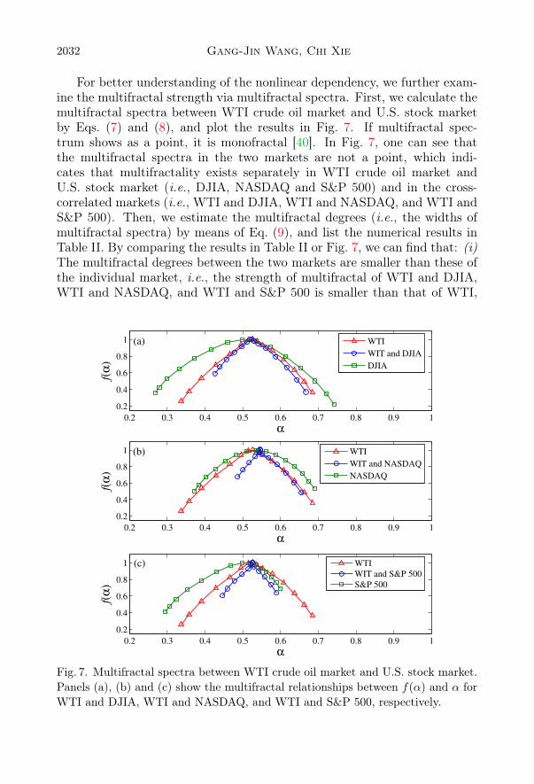
For better understanding of the nonlinear dependency, we further exam-ine the multifractal strength via multifractal spectra. First, we calculate themultifractal spectra between WTI crude oil market and U.S. stock marketby Eqs. (7) and (8), and plot the results in Fig. 7. If multifractal spec-trum shows as a point, it is monofractal [40]. In Fig. 7, one can see thatthe multifractal spectra in the two markets are not a point, which indi-cates that multifractality exists separately in WTI crude oil market andU.S. stock market (i.e., DJIA, NASDAQ and S&P 500) and in the cross-correlated markets (i.e., WTI and DJIA, WTI and NASDAQ, and WTI andS&P 500). Then, we estimate the multifractal degrees (i.e., the widths ofmultifractal spectra) by means of Eq. (9), and list the numerical results inTable II. By comparing the results in Table II or Fig. 7, we can find that: (i)The multifractal degrees between the two markets are smaller than these ofthe individual market, i.e., the strength of multifractal of WTI and DJIA,WTI and NASDAQ, and WTI and S&P 500 is smaller than that of WTI,

0.2 0.3 0.4 0.5 0.6 0.7 0.8 0.9 1

0.2

0.4

0.6

0.8

1

α

f(α

)

(a)

0.2 0.3 0.4 0.5 0.6 0.7 0.8 0.9 1

0.2

0.4

0.6

0.8

1

α

f(α

)

(b)

0.2 0.3 0.4 0.5 0.6 0.7 0.8 0.9 1

0.2

0.4

0.6

0.8

1

α

f(α

)

(c)

WTI

WIT and DJIA

DJIA

WTI

WIT and NASDAQ

NASDAQ

WTI

WIT and S&P 500

S&P 500

Fig. 7. Multifractal spectra between WTI crude oil market and U.S. stock market.Panels (a), (b) and (c) show the multifractal relationships between f(α) and α forWTI and DJIA, WTI and NASDAQ, and WTI and S&P 500, respectively.

Cross-correlations Between WTI Crude Oil Market and U.S. Stock Market . . . 2033

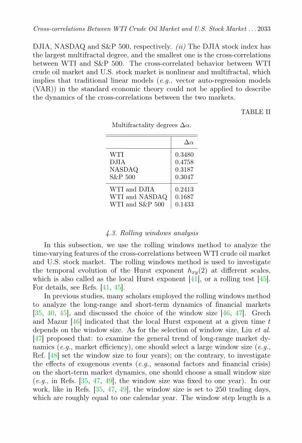
DJIA, NASDAQ and S&P 500, respectively. (ii) The DJIA stock index hasthe largest multifractal degree, and the smallest one is the cross-correlationsbetween WTI and S&P 500. The cross-correlated behavior between WTIcrude oil market and U.S. stock market is nonlinear and multifractal, whichimplies that traditional linear models (e.g., vector auto-regression models(VAR)) in the standard economic theory could not be applied to describethe dynamics of the cross-correlations between the two markets.

TABLE II

Multifractality degrees ∆α.

∆α

WTI 0.3480DJIA 0.4758NASDAQ 0.3187S&P 500 0.3047

WTI and DJIA 0.2413WTI and NASDAQ 0.1687WTI and S&P 500 0.1433

4.3. Rolling windows analysis

In this subsection, we use the rolling windows method to analyze thetime-varying features of the cross-correlations between WTI crude oil marketand U.S. stock market. The rolling windows method is used to investigatethe temporal evolution of the Hurst exponent hxy(2) at different scales,which is also called as the local Hurst exponent [41], or a rolling test [45].For details, see Refs. [41, 45].

In previous studies, many scholars employed the rolling windows methodto analyze the long-range and short-term dynamics of financial markets[35, 40, 45], and discussed the choice of the window size [46, 47]. Grechand Mazur [46] indicated that the local Hurst exponent at a given time tdepends on the window size. As for the selection of window size, Liu et al.[47] proposed that: to examine the general trend of long-range market dy-namics (e.g., market efficiency), one should select a large window size (e.g.,Ref. [48] set the window size to four years); on the contrary, to investigatethe effects of exogenous events (e.g., seasonal factors and financial crisis)on the short-term market dynamics, one should choose a small window size(e.g., in Refs. [35, 47, 49], the window size was fixed to one year). In ourwork, like in Refs. [35, 47, 49], the window size is set to 250 trading days,which are roughly equal to one calendar year. The window step length is a

2034 Gang-Jin Wang, Chi Xie

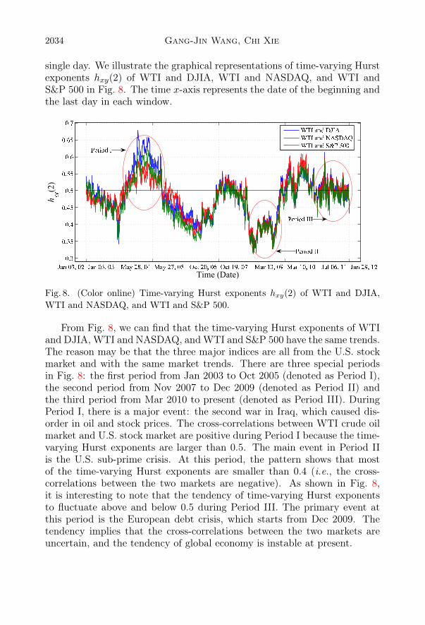
single day. We illustrate the graphical representations of time-varying Hurstexponents hxy(2) of WTI and DJIA, WTI and NASDAQ, and WTI andS&P 500 in Fig. 8. The time x-axis represents the date of the beginning andthe last day in each window.

Fig. 8. (Color online) Time-varying Hurst exponents hxy(2) of WTI and DJIA,WTI and NASDAQ, and WTI and S&P 500.

From Fig. 8, we can find that the time-varying Hurst exponents of WTIand DJIA, WTI and NASDAQ, andWTI and S&P 500 have the same trends.The reason may be that the three major indices are all from the U.S. stockmarket and with the same market trends. There are three special periodsin Fig. 8: the first period from Jan 2003 to Oct 2005 (denoted as Period I),the second period from Nov 2007 to Dec 2009 (denoted as Period II) andthe third period from Mar 2010 to present (denoted as Period III). DuringPeriod I, there is a major event: the second war in Iraq, which caused dis-order in oil and stock prices. The cross-correlations between WTI crude oilmarket and U.S. stock market are positive during Period I because the time-varying Hurst exponents are larger than 0.5. The main event in Period IIis the U.S. sub-prime crisis. At this period, the pattern shows that mostof the time-varying Hurst exponents are smaller than 0.4 (i.e., the cross-correlations between the two markets are negative). As shown in Fig. 8,it is interesting to note that the tendency of time-varying Hurst exponentsto fluctuate above and below 0.5 during Period III. The primary event atthis period is the European debt crisis, which starts from Dec 2009. Thetendency implies that the cross-correlations between the two markets areuncertain, and the tendency of global economy is instable at present.

Cross-correlations Between WTI Crude Oil Market and U.S. Stock Market . . . 2035

5. Conclusions

In summary, we examine the cross-correlations between WTI crude oilmarket and U.S. stock market. We choose the three major U.S. stock indices(i.e., DJIA, NASDAQ and S&P 500) as the research objects. Or rather, inthis study, we investigate the cross-correlations between WTI and DJIA,WTI and NASDAQ, and WTI and S&P 500. In the empirical process, wefirst use a statistical test proposed by Podobnik et al. [41] to test the pres-ence of cross-correlations qualitatively and find that the cross-correlationssignificantly exist between WTI and DJIA, WTI and NASDAQ, and WTIand S&P 500. Then, we employ MF-DCCA method to examine the pres-ence of cross-correlations quantitatively and find that the cross-correlatedbehaviors between crude oil market and U.S. stock market are nonlinearand multifractal. Finally, we use the rolling windows approach to capturethe dynamics of cross-correlations and find that there are three special pe-riods whose time-varying Hurst exponents are different from the others.

This work was supported by the National Social Science Foundation ofChina (Grant No. 07AJL005), the National Soft Science Research Programof China (Grant No. 2010GXS5B141), the Program for Changjiang Scholarsand Innovative Research Team in University (Grant No. IRT0916), the Sci-ence Fund for Innovative Groups of Natural Science Foundation of HunanProvince of China (Grant No. 09JJ7002), and the Foundation for Innova-tive Research Groups of the National Natural Science Foundation of China(Grant No. 71221001).

REFERENCES

[1] R.N. Mantegna, H.E. Stanley, An Introduction to Econophysics: Correlationsand Complexity in Finance, Cambridge University Press, Cambridge 2000.

[2] J. Kwapień, S. Drożdż, Phys. Rep. 515, 115 (2012).[3] E.L. Siqueira et al., Physica A 389, 2739 (2010).[4] L. Kilian, C. Park, Int. Econ. Rev. 50, 1267 (2009).[5] M.C. Jones, G. Kaul, J. Financ. 51, 463 (1996).[6] S.S. Chen, Energ. Econ. 32, 490 (2009).[7] G. Filis, Energ. Econ. 32, 877 (2010).[8] M.H. Berument et al., Energ. J. 31, 149 (2010).[9] M.A.M. Al Janabi et al., Int. Rev. Financ. Anal. 19, 47 (2010).[10] R.-G. Cong et al., Energ. Policy 36, 3544 (2008).[11] C. Ciner, Stud. Nonlinear Dyn. E5, 203 (2001).[12] E.F. Fama, J. Financ. 25, 383 (1970).

2036 Gang-Jin Wang, Chi Xie

[13] R.N. Mantegna, H.E. Stanley, Nature 376, 46 (1995).[14] D.O. Cajueiro, B.M. Tabak, Physica A 342, 656 (2004).[15] B. Podobnik et al., Physica A 362, 465 (2006).[16] R.N. Mantegna, Eur. Phys. J. B11, 193 (1999).[17] J. Kwapień et al., Acta Phys. Pol. B 40, 175 (2009).[18] G.-J. Wang et al., Physica A 391, 4136 (2012).[19] V. Plerou et al., Phys. Rev. Lett. 83, 1471 (1999).[20] Z. Burda et al., Acta Phys. Pol. B 34, 87 (2003).[21] S. Drozdz et al., Acta Phys. Pol. B 38, 4027 (2007).[22] B.B. Mandelbrot, The Fractal Geometry of Nature, Freeman, New York 1982.[23] J.W. Kantelhardt et al., Physica A 316, 87 (2002).[24] Y. Yuan et al., Physica A 391, 3484 (2012).[25] P. Oświęcimka et al., Acta Phys. Pol. B 36, 2447 (2005).[26] Ł. Czarnecki, D. Grech, Acta Phys. Pol. A 117, 623 (2010).[27] P. Oświęcimka et al., Acta Phys. Pol. A 117, 637 (2010).[28] M. Bolgorian, Z. Gharli, Acta Phys. Pol. B 42, 159 (2011).[29] D. Ghosh et al., Acta Phys. Pol. B 43, 1261 (2012).[30] C.K. Peng et al., Phys. Rev. E49, 1685 (1994).[31] B. Podobnik, H.E. Stanley, Phys. Rev. Lett. 100, 084102 (2008).[32] G.F. Zebende, Physica A 390, 614 (2010).[33] A.J. Lin et al., Nonlinear Dynam. 67, 425 (2012).[34] W.-X. Zhou, Phys. Rev. E77, 066211 (2008).[35] Y.D. Wang et al., Physica A 389, 5469 (2010).[36] L.-Y. He, S.-P. Chen, Chaos Soliton. Fract. 44, 355 (2011).[37] Y.D. Wang et al., Physica A 390, 864 (2011).[38] L.-Y. He, S.-P. Chen, Physica A 390, 297 (2011).[39] Z.H. Li, X.S. Lu, Physica A 391, 3930 (2012).[40] G.X. Cao et al., Physica A 391, 4855 (2012).[41] B. Podobnik et al., Eur. Phys. J. B71, 243 (2009).[42] P. Oświęcimka et al., Physica A 347, 626 (2005).[43] B. Podobnik et al., PNAS 106, 22079 (2009).[44] G.M. Ljung, G.E.P. Box, Biometrika 65, 297 (1978).[45] L.-Y. He et al., Physica A 391, 3770 (2012).[46] D. Grech, Z. Mazur, Physica A 336, 133 (2004).[47] L. Liu, J.Q. Wan, Physica A 390, 3754 (2011).[48] D.O. Cajueiro, B.M. Tabak, Physica A 346, 577 (2005).[49] Y.D. Wang et al., Physica A 390, 817 (2011).