Time Series Modelling of Monthly WTI Crude Oil Returns

Time Series Modelling ofMonthly WTI Crude Oil Returns

Derek LAM

Lincoln College

University of Oxford

A thesis submitted in partial fulfilment for the degree of Master ofScience in Mathematical and Computational Finance

Trinity 2013

Acknolwedgements

First of all, I would like to express my sincere gratitude to my thesis supervisor,Dr. Patrick McSharry, for his valuable guidances and advices. I would also like tothank all of the lecturers I have met this year, for without them, I would never beable to learn so much this year. Lastly, I would like to thank my parents for theirunlimited support all along.

Abstract

This paper examines the dynamics of the monthly WTI crude oil return for thepast two decades. The data are divided into two ten-year periods, and we ex-plore with two approaches. We first build univariate time series models using theBox-Jenkins methodology. Techniques such as stationarity tests and autocorrela-tion plots are used to determine the orders of the final ARIMA model. GARCHand APARCH are also used to model residuals. Then, we build regression modelsbased on eight explanatory variables. They are consumption, production, endingstock, net import, refinery utilisation rate, U.S. interest rate, NYMEX oil futurescontract 4 and S&P 500 index. Stepwise AIC method is employed to determine theoptimal variables to be included. Multicollinearity is not evident in the reducedmodels. Residual analysis suggests that the assumptions of linear regression arenot violated. Lastly, the forecasting powers of the models are compared. GARCHand APARCH perform the best in terms of forecasting accuracy, with APARCHperforming the best in a turbulent market.

Keywords: Linear regression, ARIMA, GARCH, APARCH, time series forecasting,residual analysis

Contents

1 Introduction 11.1 Brief History of WTI crude oil for the past 20 years . . . . . . . . . 1

2 Box-Jenkins approach 22.1 ARIMA . . . . . . . . . . . . . . . . . . . . . . . . . . . . . . . . . 22.2 Innovation modeling . . . . . . . . . . . . . . . . . . . . . . . . . . 52.3 Forecasting . . . . . . . . . . . . . . . . . . . . . . . . . . . . . . . 6

3 Empirical results of univariate approach 83.1 ARIMA fits . . . . . . . . . . . . . . . . . . . . . . . . . . . . . . . 83.2 Residual analysis and GARCH/APARCH fits . . . . . . . . . . . . 12

4 Linear regression approach 184.1 Stepwise AIC approach towards model selection . . . . . . . . . . . 184.2 Estimation of regression parameters . . . . . . . . . . . . . . . . . . 20

5 Empirical results of linear regression approach 215.1 Fitting explanatory variables . . . . . . . . . . . . . . . . . . . . . . 215.2 Residual analysis . . . . . . . . . . . . . . . . . . . . . . . . . . . . 27

6 Conclusion 296.1 Forecasting comparison . . . . . . . . . . . . . . . . . . . . . . . . . 296.2 Concluding remarks . . . . . . . . . . . . . . . . . . . . . . . . . . . 29

7 R codes 31

References 38

1 Introduction

Crude oil is one of the most important commodities in the world. Its applicationsare ubiquitous in daily life, from making detergents and plastic bags to fuelingcars and ships. Despite being non-renewable, the world consumes crude oil everysingle minute as it is difficult to find an alternative source that can parallel itsperformances. With such a uniqueness in the world, it is vital for us to developa better understanding of its price dynamics, so that the myriad industries whichconsume or supply oils can make more informed decisions.

In this paper, we will explore two feasible approaches towards building models.The first is a time series approach, aiming at building ARIMA-GARCH/APARCHmodels, using the Box-Jenkins methodology. The second is to seek a set of mean-ingful explanatory variables and build linear regression models. We will compareand contrast the forecasting accuracy of these models.

1.1 Brief History of WTI crude oil for the past 20 years

Modelling the dyanmics of crude oil is not easy because its price may fluctuatefrom time to time unpredictably and may also depend on a lot of factors. Forthe past two decades, oil has been experiencing some ups and downs. In early1999 (See Figure 1), there was the Asian Financial Crisis, along with Iraq decidingto increase oil production, which caused oil prices to reach a bottom. But themarket adjusted quickly and reached over U.S.$ 34 by late 2000. The dotcombubble in 2001 caused another round of economic panic, which caused it to dropuntil early 2002. Then, the global economy had been regaining momentum whichresulted in a few years of bullish state. Accordingly, oil prices had been spikingup. Other contributing factors included limiting amount of global oil supply andhostile relationships between the U.S. and a number of oil producer countries. Oilprice touched an all-time high of U.S.$ 147.30 in which the housing bubble inthe U.S. started to burst, and a unprecedented credit crisis was followed. Thedramatic decline in oil price that followed was difficult to model. Even though theprice had, in general, exhibited a steady level of recovery after the financial crisisin 2008, it still posts a great challenge to find a model that performs consistentlywell, when being confronted with such unpredictable circumstances.

1

2 Box-Jenkins approach

2.1 ARIMA

We begin by exploring the ARIMA-Box Jenkins methodology, proposed by G. Boxand G. Jenkins[1], to build a univariate time series forecasting model. It is oneof the most common ways to formulate a forecasting model for a univariate timeseries such as the monthly WTI crude oil spot prices we intend to model. Tounderstand what this methodology entails, we first define what is meant by anARMA (and hence ARIMA) model.

Definition 2.1 (ARMA). An ARMA (Autoregressive Moving Average) (p, q)model of a time series Yt has the following form:

Yt = φ0 +

p∑i=1

φiYt−i +

q∑j=1

θjεt−j + εt (1)

1. p refers to the number of autoregressive terms

2. q refers to the number of lagged error terms

3. φ refers to the coefficients of the autoregressive terms and the constant

4. θ refers to the coefficients of the moving average terms

Definition 2.2 (White noise). The εt defined above is a white noise process,meaning that it is a sequence of variables which have mean zero, variance σ2, andzero correlation across time, i.e. E(εuεv) = 0 if u 6= v. They are also independentand identically distributed.

An ARIMA model is an extension of the ARMA class.

Definition 2.3 (ARIMA). A time series Yt is said to be of the ARIMA (Autore-gressive Integrated Moving Average) format if∇dYt is a stationary ARMA process,where d refers to the number of difference to be taken on the original series.

However, in reality, it is common to model log returns instead of prices infinancial time series. This is defined as the difference between current and previouslog prices. To determine whether a log transformation is needed, with aims suchas stabilising variance or creating a more Gaussian distributed set of data, we havethe following procedure:

2

Definition 2.4 (Box-Cox transformation). For each y, we can use the Box-Coxtransformation and convert it into y(λ), where

y(λ) − 1

λ, if λ 6= 0 (2)

log(y), if λ = 0 (3)

Accordingly, we can plot, with respect to the 95% confidence interval, a log-likelihood graph for the feasible values of λ.

In the Box-Jenkins approach, we also need to ensure the series is stationary,i.e. it has approximately constant mean and variance. This can be done bydifferencing the series several times (at most twice usually). The AugmentedDickey-Fuller Test[9] will be performed to see if the transformed series is stationary.This provides an alternative methodology to check for stationarity other thanobserving the plotted series itself.

Definition 2.5 (Augmented Dickey-Fuller Test). It is a test to see if a time serieshas a unit root. If it does, the series is considered non-stationary. The nullhypothesis here is that the time series is non-stationary.

After that, we try to plot the autocorrelation and partial correlation functionsagainst different lags in order to determine the appropriate orders of p and q forour model. The expected patterns are summarised in the following:

AR(p) MA(q) ARMA(p,q)ACF Tails off Cuts off after lag q Tails off

PACF Cuts off after lag p Tails off Tails off

Sometimes, there may be more than one potential candidate for the final model.In this case, we may want to use an alternative approach based on information cri-teria to select the most approriate model. One way is to employ the AIC (AkaikeInformation Criterion) measure [10].

Definition 2.6 (AIC). AIC measures how well the estimated model fits with thedata relative to the other models, and is calculated using the formula below:

AIC(p, q) = −2log(L) + 2(p+ q), (4)

where L is the maximum value of the likelihood function of the ARMA(p,q) model,and p+q is the total number of parameters found in it. The recommended modelunder this approach is then the one with the smallest AIC value. Therefore, wewant p+q to be small and L to be large. In other words, the approach encouragesboth goodness of fit and parsimony.

3

Once the model is specified, we employ the maximum likelihood estimationmethod to estimate the respective coefficients for the autoregressive and movingaverage terms. Finally, we perform model diagnostics to see if the estimatedmodel is consistent with the specifications of a univariate time series process withstationarity. Graphically, we can employ the following plot:

Definition 2.7 (Normal QQ plot). This refers to a plot of the quantiles of themodel residuals against the quantiles of a Normal Distribution. On this plot thereis a QQ line which represents a perfect match between model residuals and theNormal distribution. If the model residuals are normally distributed, they shouldbe plotted along this line.

Also, we can perform the McLeod-Li test and the Jarque-Bera test on theresiduals.

Definition 2.8 (McLeod-Li test). The McLeod-Li test[12] is based on the sampleautocorrelations of the squared time series. It has the following form:H0: The residuals are independent.H1: The resdiauls are dependent.

L = (n2 + 2n)K∑k=1

ρ2kn− k

, (5)

ρk =

n∑t=k+1

(ε2t − σ2n)(ε2t−k − σ2

n)

n∑t=1

(ε2t − σ2n)

, σ2n =

n∑t=1

ε2t

n,

Provided that Yt is a series of identical and independently distributed sequence,the statistic L should have a distribution of χ2(K) asymptotically. If we apply thetest to the residuals of the fitted ARIMA model and that the returned p-values arebelow 0.05, we have strong evidence to reject the null hypothesis that all laggedautocorrelations up to lag k are zero.

Definition 2.9 (Jarque-Bera test). The Jarque-Bera test[11] can be defined inthe following with test statistic L.H0: The residuals are normally distributed.H1: The residuals do not follow a normal distribution.

L =n

6(S2 + 0.25(K − 3)2), (6)

where n is the number of data, S is the sample skewness and K is the samplekurtosis. If the data come from a normal distribution, the statistic L should havethe asymptotic distribution of a χ2(2) distribution.

4

If the residuals violate our assumptions, we will resort to the GARCH (Gener-alised Autoregressive Conditional Heteroskedasticity) methodology to model theresiduals.

2.2 Innovation modeling

In residual analysis of financial time series, Generalised Autoregressive ConditionalHeteroskedasticity (GARCH) models, proposed by Bollerslev in 1986[6], are widelyused to specify and model innovations, i.e. the differences between the fitted valuesof the proposed model and the observed values. They have the ability to model thephenomenon of volatility clustering seen in many financial time series data. Theyevolve from the Autoregressive Conditional Heteroskedasticity (ARCH) model,proposed by Engle in 1982[5], which assumes the variance of the current innovationto be dependent on error terms of the previous time periods.

Definition 2.10 (ARCH). ARCH(q) models, where q refers to the order of thelagged autoregressive terms of previous innovations, have the following term:

εt = σtzt, zt white noise,

σ2t = ω +

q∑i=1

αiε2t−i, ω > 0, αi ≥ 0, i > 0 (7)

Definition 2.11 (GARCH). On the other hands, GARCH models assume theconditional variances of innovations follow an ARMA model. In that case, aGARCH(p, q) model, where p and q are the orders of the GARCH and ARCHterms respectively, refers to σt having the following term:


σ2t = ω +

q∑i=1

αiε2t−i +

p∑i=1

βiσ2t−i, ω > 0, αi ≥ 0, βi ≥ 0, i > 0 (8)

Also, we need to imposeq∑i=1

αi +p∑i=1

βi < 1 to ensure stationarity. We note that

GARCH will collapse to ARCH if p=0.

Also, we can definte APARCH[8], which is another generalised conditionalheteroskedasticity model with the special feature that can account for asymmetriceffects of volatilities. It is defined in the following:

Definition 2.12 (APARCH).


5

σδt = ω +

q∑i=1

αi(|εt−i|+ γiεt−i)δ +

p∑i=1

βiσδt−i, ω > 0, αi ≥ 0, βi ≥ 0, i > 0 (9)

To seek for the right GARCH/APARCH model, we plot squared residualsof the fitted model and their acf and pacf. Apply the same procedure to findout until we find a GARCH/APARCH(p,q) model on the squared residuals suchthat the AIC value is the smallest. Altogether, we will have the fitted ARIMA-GARCH/APARCH models for forecasting future values.

2.3 Forecasting

Definition 2.13 (n-step ahead forecast). The one-step ahead forecast of Yt+1

based on an ARMA-GARCH model is defined as

Yt(1) = E(Yt+1|Yt, Yt−1...) = φ0 +

p∑i=1

φiYt+1−i +

q∑j=1

θjεt+1−j, (10)

where the εs follow the stated GARCH model. Recursively, we can then define then-step ahead forecast of Yt(n) for any n.

We can employ two major statistical measures for comparing forecast accuracy.They are the MSE and the MAE respectively.

Definition 2.14 (Mean squared error). It computes the squared difference be-tween every forecasted value and every realised value of the quantity being esti-mated, and finds the mean of them afterwards. One can interpret it literally asthe average of the squares of errors. Assume Yj as the j-step ahead realised value,the error has the following formula:

MSE =1

n

n∑j=1

((Yt(j)− Yj)2) (11)

Definition 2.15 (Mean absolute error). It computes the mean of all the absolute,instead of squared, forecast errors. The formula is the following:

MAE =1

n

n∑j=1

(|Yt(j)− Yj|) (12)

Although both ways are closely related, MAE is more popular in use as it doesnot require squaring, hence it is considered easier to implement. However, MSEmay perform better in some occassions. For example, assume we have two differentmodels: one has 10 error values with the first nine equal to 1 and the remaining

6

one equal to 11; the other also has 10 error values which are all equal to 2. In thisparticular case, we have equal MAE (both equal to 2) but the MSE are totallydifferent (13 against 4). The second model is clearly preferred. Therefore, oneshould compute both metrics to obtain a better picture of the forecasting powersof various models.

7

3 Empirical results of univariate approach

WTI (West Texas Intermediate) crude oil, along with Brent crude oil, is widelyconsidered as one of the benchmarks for understanding oil price dynamics. Manytrades and derivatives are based on its prices. In this paper, we obtain the datafrom the U.S. EIA (Energy Information Administration) where monthly spot pricesof the WTI oil are available. The time frame we choose spans between April 1993and March 2013, i.e. 20 years of data. The monthly frequency is chosen as this isthe smallest unit of frequency available for all variables. We then further dividethe time frame into two 10-year periods, with the first nine years of data in eachperiod used for model construction and the last year validating forecast accuracy.In particular, we can see that, although oil prices do experience ups and downsin the first period, the second period suffers a much larger scale of fluctuations,especially during 2008, the year when the financial crisis happened. Therefore, weshould examine if there is a structual change in the oil market from one period toanother.

Time

Month

ly WT

I spo

t pric

e US$

1995 2000 2005 2010

2040

6080

100

120

Figure 1: Time series plot of monthly WTI spot price from Apr 1993 to Mar 2002(1st period, left) and from Apr 2003 to Mar 2012 (2nd period, right)

3.1 ARIMA fits

We first attempt to see if a log transformation is recommended by plotting theBox-Cox log likelihood graphs. As λ = 0 falls within the 95% confidence intervalfor both periods, we adopt such a transformation. From Figure 2, we can see

8

clearly that both series are still clearly non-stationary.

-0.5 0.0 0.5

0.00.2

0.40.6

0.81.0

Relative Likelihood Analysis95% Confidence Interval

λ

R(λ)

λ = 0.056

-0.8 -0.4 0.0 0.40.0

0.20.4

0.60.8

1.0

Relative Likelihood Analysis95% Confidence Interval

λ

R(λ)

λ = -0.166

Figure 2: Box-Cox likelihood plots for period 1(left) and 2(right)

Time

Month

ly WT

I spo

t pric

e US$

1995 2000 2005 2010

2.53.0

3.54.0

4.5

Figure 3: Time series plot of monthly WTI log price in period 1 (left) and 2 (right)

The Augmented Dickey-Fuller test for stationarity suggests a p-value of 0.47and 0.09 respectively, hence we cannot reject the null hypothesis at the 5% sig-nificant level. We try working on log return instead. The formula for log return

9

is Lt = log( Pt

Pt−1). This time, we see that the ADF test provides p-values smaller

than 0.01 in both periods, suggesting stationary in the series, which can also beconfirmed by looking at Figure 4.

Time

Month

ly WT

I spo

t pric

e US$

1995 2000 2005 2010

-0.3

-0.2

-0.1

0.00.1

0.2

Figure 4: Monthly log returns of WTI crude oil in period 1 (left) and 2 (right)

Then, we start working on modeling the autoregressive (AR) and moving av-erage (MA) orders respectively.

0 5 10 15 20

-0.2

0.00.2

0.40.6

0.81.0

Series as.vector(log.return1)

Lag

ACF

5 10 15 20

-0.2

-0.1

0.00.1

0.2

Lag

Partia

l ACF


Figure 5: ACF and PACF plots for period 1

10

For period 1, we see no significant spikes in either plot, except at lag 15 whereit is slightly below the lower confidence bound. ARMA(0,0) (random walk) modelseems to be a potential candidate here.

0 5 10 15 20

-0.2

0.00.2

0.40.6

0.81.0


Lag

ACF

5 10 15 20

-0.2

-0.1

0.00.1

0.20.3

Lag

Partia

l ACF


Figure 6: ACF and PACF plots for period 2

For period 2, spikes seem to be more significant up to lag 2 in both plots. Thissuggest an ARMA (2,2) model should be postulated as a potential fitted model.Then, we compare the various AIC values generated by fitting different p and q,where they range from 0 to 2, and conclude a ARMA(0,1) model and a ARMA(2,2)model for the monthly log return of WTI crude oil in the 1st and the 2nd periodrespectively. In particular, if we increase either order by 1 in the ARMA (2,2)model, we get higher AIC values (-220.9 and -214.7), resulting in overfitting. Be-low are the table of AIC values.

Order (0,0) (0,1) (0,2) (1,0) (1,1) (1,2) (2,0) (2,1) (2,2)

AIC -249.8 -250.0 -248.1 -249.9 -248.3 -246.3 -248.0 -245.9 -244.5

AIC -208.9 -213.2 219.0 -216.1 -216.4 -217.7 -218.7 -217.0 -222.4

Table 1: AIC table for various orders

11

3.2 Residual analysis and GARCH/APARCH fits

We first look at the plots of model residuals across the two periods. They both lookreasonably stationary and seem to evolve around a mean of zero. We should alsonote that, during the financial crisis, we see some relatively large model residuals.We then proceed to plot their ACFs and PACFs.

Time

model1$resid

1994 1998 2002

-0.2

-0.1

0.00.1

0.2

Time

model2$resid

2004 2008 2012

-0.2

-0.1

0.00.1

Figure 7: Residual plots for model 1 and 2

0 5 10 15 20

-0.2

0.00.2

0.40.6

0.81.0

Series as.vector(model1$resid)

Lag

ACF

5 10 15 20

-0.2

-0.1

0.00.1

0.2

Lag

Partia

l ACF


Figure 8: ACF and PACF plots for residuals of model 1

12

0 5 10 15 20

-0.2

0.00.2

0.40.6

0.81.0

Series as.vector(model1$resid^2)

Lag

ACF

5 10 15 20

-0.2

-0.1

0.00.1

0.2

LagPa

rtial A

CF

Series as.vector(model1$resid)^2

Figure 9: ACF and PACF plots for squared residuals of model 1

0 5 10 15 20

-0.2

0.00.2

0.40.6

0.81.0


Lag

ACF

5 10 15 20

-0.2

-0.1

0.00.1

0.2

Lag

Partia

l ACF


Figure 10: ACF and PACF plots for residuals of model 2

13

0 5 10 15 20

-0.2

0.00.2

0.40.6

0.81.0

Series as.vector(model2$resid^2)

Lag

ACF

5 10 15 20

-0.2

-0.1

0.00.1

0.20.3

LagPa

rtial A

CF

Series as.vector(model2$resid)^2

Figure 11: ACF and PACF plots for squared residuals of model 2

As expected, there is no significant autocorrelation for the residuals across anylag in either period. For period 1, there is no particularly significant spikes in anylag. For period 2, lag 2 seems to catch our attention for the ACF and PACF ofthe squared residuals.

-2 -1 0 1 2

-0.2

-0.1

0.00.1

0.2

Normal Q-Q Plot

Theoretical Quantiles

Samp

le Qu

antile

s

-2 -1 0 1 2

-0.2

-0.1

0.00.1

Normal Q-Q Plot


Samp

le Qu

antile

s

Figure 12: Normal QQ plots for model 1 and 2

The normal QQ-plots suggest strong evidence of normality for period 1, but

14

only a mild evidence for period 2. However, the Jarque-Bera test suggests a p-value of 0.9932 and 0.1492 respectively, so we cannot reject the null hypothesisthat the residuals are normally distributed.

5 10 15 20

0.0

0.2

0.4

0.6

0.8

1.0

Lag

P-value

5 10 15 20

0.0

0.2

0.4

0.6

0.8

1.0

Lag

P-value

Figure 13: Mcleod.Li test results plotted for period 1(left) and 2(right)

On the other hand, the McLeod-Li test suggests a strong evidence that theresiduals for period 2 are autocorrelated. The plots of the p-values against differentlags indicate that from lag 2 onwards in the second period, all p-values lie belowthe 0.05 threshold. This is a stark contrast to what we see in the first period,where all values lie way above the threshold. Therefore, a GARCH model may beappropriate to fit the second set of data. The intuitive rationale behind that ispossibly linked to the fact that the financial crisis has brought in some significanteffects of volatility clustering. We then loop through a set of AIC values for variousorders of GARCH model, and we see that a GARCH(1,1) model provides the lowestvalue (-234.5455). To validate the choice, we plot the residuals of the GARCH(1,1)model for period 2 in Figure 14 and 15. We notice that all the significant spikesare removed, confirming the adequacy of the model.

15

0 5 10 15 20

-0.2

0.00.2

0.40.6

0.81.0

Series model.garch2.res

Lag

ACF

5 10 15 20

-0.2

-0.1

0.00.1

0.2

LagPa

rtial A

CF

Series model.garch2.res

Figure 14: ACF and PACF plots of residuals of GARCH(1,1) model for period 2

0 5 10 15 20

-0.2

0.00.2

0.40.6

0.81.0

Series model.garch2.res^2

Lag

ACF

5 10 15 20

-0.2

-0.1

0.00.1

0.2

Lag

Partia

l ACF

Series model.garch2.res^2

Figure 15: ACF and PACF plots of squared residuals of GARCH(1,1) model forperiod 2

Our finalised are therefore presented below. For comparison purpose, we havealso included an APARCH(1,1) fit to the residuals. We will evaluate their fore-casting powers later.

16

Order AR(1) AR(2) MA(1) MA(2) GARCH(1) ARCH(1)1st period 0.152nd period 0.62 -0.24 -0.53 0.38 0.18 0.57

Order AR(1) AR(2) MA(1) MA(2) APARCH(1) ARCH(1)2nd period 0.65 -0.30 -0.58 0.41 0.07 0.58

Table 2: Parameters for fitted models

17

4 Linear regression approach

4.1 Stepwise AIC approach towards model selection

Linear models can be used both to describe the statistical relationships betweenresponse variable and a list of explanatory variables, and to make predictionsregarding the response variable.

Let p be the number of explanatory variables and n be the number of observa-tions for each variable. In a linear regression, we have that yi = β1x1,i + β2x2,i +...+βpxp,i+εi, where y and xis refer to response variable and explanatory variablesrespectively. It is also convenient to express the relationship in matrix form,

Y = Xβ + ε, (13)

Y = (y1, ..., yn)T ,

X =

1 x1,1 ... xp,11 x1,2 ... xp,2...

... ......

1 x1,n−1 ... xp,n−1

1 x1,n ... xp,n

,

β = (β1, ..., βp)T ,

ε = (ε1, ...εn)T

In fitting a linear regression model, our goal here is to derive a set of estimatedβ. First, we need to make a few major assumptions:

1. Linearity. This means that the mean of the response variable is a linearcombination of the regression coefficients and the explanatory variables. Inmathematical terms, this essentially means we need E(Y ) = XTβ.

2. Absence of multicollinearity among explanatory variables. In math-ematical terms, this means we need the columns of X to be linearly indepe-dent and form a basis of the matrix. This way, we can guarantee a vectorof regression coefficients exists. However, this may be violated if we includevariables that exhibit perfect correlation. In reality, it is rare to have a cor-relation number of 1 or -1 between two variables. We decide to follow [15],and define 0.75 as the threshold. Any absolute correlation number abovethat is considered as perfect or near-perfect correlation.

18

3. Precision of data. Here, we need our data collected for all variables to beaccurate so that we can treat them as deterministic values. We believe EIAshould be a reliable source of information and we assume the validility ofthis point.

4. Homoscedasticity. This means we have constant variances in residuals.A plot of standardised residuals and model fitted values should review ascattered distribution if this is the case.

5. Uncorrelated errors. This assumes that the errors of the response vari-ables are indepedent of each other.

6. Normality of errors with zero mean. This can be verified by normalQQ-plots, just like what we did for the univariate time series analysis. As forthe mean, we just sum all the residuals and divide them by the total numberof errors to see if the value is close to zero.

Here, we recall Akaike Information Criterion (AIC)[10] as a measure to deter-mine which orders of autoregressive and moving average terms we include in thefinal model. This can be similarly adopted in regression model selection. Thedefinition here is slightly modified:

Definition 4.1 (Akaike Information Criterion for linear regression). Let RSS bethe residual sum of squares, i.e. RSS=(Y −Xβ)T (Y −Xβ). Then, we have

AICLR = nlog(RSS

n) + 2p, (14)

Below are three approaches that make use of the metric:

1. Forward selection: fit the null model, add each term separately, keep theone that reduces AIC the most, use this as the base model, add each of theother terms separately, keep the one that reduces AIC the most, repeat untilreduction in AIC is no longer significant.

2. Backward elimination: fit the full model, remove the term that reducesAIC the least, use this as the base model, remove the next term that reducesAIC the least, repeat until any further reduction in AIC is significant.

3. Stepwise selection: this is a combination of the above approaches. Wedetermine at every time whether any term can be dropped or added. Ifthe answer is no, the model is complete. This can be better than forwardselection since the initial estimate is hardly correct. Also, it can be cho-sen over backward elimination, since the full model may sometimes be toocomplicated to fit.

19

4.2 Estimation of regression parameters

Once we select the right model, we proceed to estimate the regression parameters.The Least Squares approach contends that we measure a β that minimises theresidual sum of sqaures, i.e.

∂

∂β(Y −Xβ)T (Y −Xβ) = 0 (15)

The partial differentiation leads to

−2XTY + 2(XTX)β = 0 (16)

Assuming X has rank p, i.e. full rank, we can reach a solution:

β = (XTX)−1XTY (17)

To validate the use of this estimator, we need to check that such β is anunbiased estimate of the true β, i.e. E(β) = β. This is shown in the following:

E(β) = E((XTX)−1XTY )

= (XTX)−1XTE(Y )

= (XTX)−1XTXβ (Assuming E(ε) = 0)

= β (18)

Once we have calculated these parameters, we can proceed to generate 12-month ahead predicted values for all explanatory variables. For example, if we haveseven explanatory variables, we will a total of 96 predicted values. We then plugthem into the regression model and predict the forecasted values of the responsevariable (monthly WTI crude oil log return in this case). Just like the univariatemodel, the model accuracy can be measured by MSE or MAE.

20

5 Empirical results of linear regression approach

5.1 Fitting explanatory variables

Many literatures have been dedicated to finding contributing factors to oil prices.We will include a list of eight fundamentals we deem relevant to explain the dy-namics of oil price returns, and their respective time series plots. These data areall gathered from the EIA. After a literature review of several relevant papers, thefollowing points are included, with their respective plots in Figure 16:

1. Consumption(Thousand barrels per day): in the field of economics,we know that equilibrium price of a particular asset, crude oil in this case, isdetermined by the intersection of its demand and supply curve. Therefore,we should include factors that may directly influence the demand curve, suchas market consumption (thousand barrels per day). This is explored in [16]and [17].

2. Production(Thousand barrels per day): similarly, increase in produc-tion should impact the supply curve (by shifting it rightwards), hence itshould play an important role in oil price determination. This is explored in[25] and [26].

3. Ending Stock(Thousand barrels): this refers to crude oil monthly endingstocks (thousand barrels) recorded by the EIA. Such stocks exist to avoid ashort run of oil in case of unpredicted events, and the impact on prices shouldbe two-folded. On one hand, it reduces dependence on current production;on the other hand, if people conceive that that there is excess supply atstorage, they may be more willing to consume crude oil. This is explored in[15] and [25].

4. Net import(Thousand barrels per day): as one of the largest oilconsumption countries in the world, the U.S. has long been importing oilsfrom other countries. Net import should serve as an indicator on how muchthe U.S. is in need of extra oils apart from internal supply, hence helpingcontribute to the determination of oil prices. This is explored in [27].

5. Refinery utilisation rate(%): here we refer to the utilisation of refinery,which is used to process crude oil into petroleum products. The numberrepresents the utilization of all crude oil distillation units. It is calculated bydividing gross inputs to these units by the operable refining capacity of theunit, which is in turn defined as the amount of capacity that, at the beginningof the period, is in operation, or those which are not in operation and notunder active repair, but capable of being placed in operation within 30 days.

21

It is essentially the total of operating and idle capacity for oil production.Ideally, a higher rate indicates a more effective use of crude oil. This hasbeen considered in [15] and [24].

6. Interest rate(%): the US Federal Funds effective monthly rates is used forthis important macroeconomic indicator. Interest rate has always been one ofthe most popular monetary tools used by government to boost the economy.Reducing its level implies a lower cost of borrowing, thereby encouragingpeople to consume and invest more. This has been considered in [18], [19]and [21].

7. NYMEX Oil Futures Contract 4 (US dollars per barrel): Themarket’s prediction of what crude oil should trade in the future should be anindicator of how it is trading at the moment. We use the NYMEX Contract4 to reflect this view since this is the longest-dated price data available foraccess. The contract expires at the 4th earliest delivery date, which is usuallythe 25th day of a month. The inclusion of oil futures is explored in [15] and[24].

8. S&P 500 index: as oil is arguably one of the most important commoditiesin the U.S., it should be very sensitive to the macroeconomic enviroments.The monthly closing of the S&P 500 index, one of the most important indi-cators of the U.S. stock market, is included for this reason. This has beenconsidered in [18] and [23].

Time

Consum

ption (0

00s bar

rels/day

)

1995 2000 2005 2010

450000

500000

550000

600000

22

Time

Produc

tion (00

0s barre

ls/day)

1995 2000 2005 2010

4000

4500

5000

5500

6000

6500

7000

Time

Ending

Stock (

000s ba

rrels)

1995 2000 2005 2010

550000

600000

650000

700000

Time

Net imp

ort (00

0s barre

ls/day)

1995 2000 2005 2010

6000

8000

10000

12000

23

Time

Utilisati

on (%)

1995 2000 2005 2010

7580

8590

95100

Time

Interest

rate (%)

1995 2000 2005 2010

01

23

45

6

Time

NYMEX

futures

contrac

t 4 (USD

/gallon)

1995 2000 2005 2010

2040

6080

100120

24

Time

S&P

500 i

ndex

1995 2000 2005 2010

400

600

800

1000

1200

1400

1600

Figure 16: Plots of various explanatory variables

We first try to fit two linear regression models based on these data. For period1, only ending stock is a significant factor at the 5% confidence level. Period2 is not much better either. Only consumption and production are consideredsignificant in the full model. We have possibly included too many variables.

Estimate Std. Error t value Pr(>|t|)(Intercept) -0.5297 0.3246 -1.63 0.1059

Consumption -0.0000 0.0000 -0.19 0.8507Production -0.0000 0.0000 -1.25 0.2154

Ending Stock 0.0000 0.0000 3.49 0.0007Net imports -0.0000 0.0000 -0.12 0.9057

Refinery utilisation rate 0.0002 0.0013 0.16 0.8764Interest rate -0.0022 0.0031 -0.70 0.4829

Futures 0.0014 0.0009 1.59 0.1157S&P 0.0000 0.0000 0.58 0.5616

Table 3: Regression model for period 1 before stepwise AIC

25


Consumption 0.0000 0.0000 2.10 0.0384Production 0.0001 0.0000 2.71 0.0079

Ending Stock 0.0000 0.0000 0.50 0.6193Net imports 0.0000 0.0000 0.35 0.7264

Refinery utilisation rate -0.0031 0.0017 -1.83 0.0702Interest rate 0.0017 0.0053 0.33 0.7427

Futures 0.0001 0.0003 0.37 0.7096S&P 0.0000 0.0000 0.19 0.8496

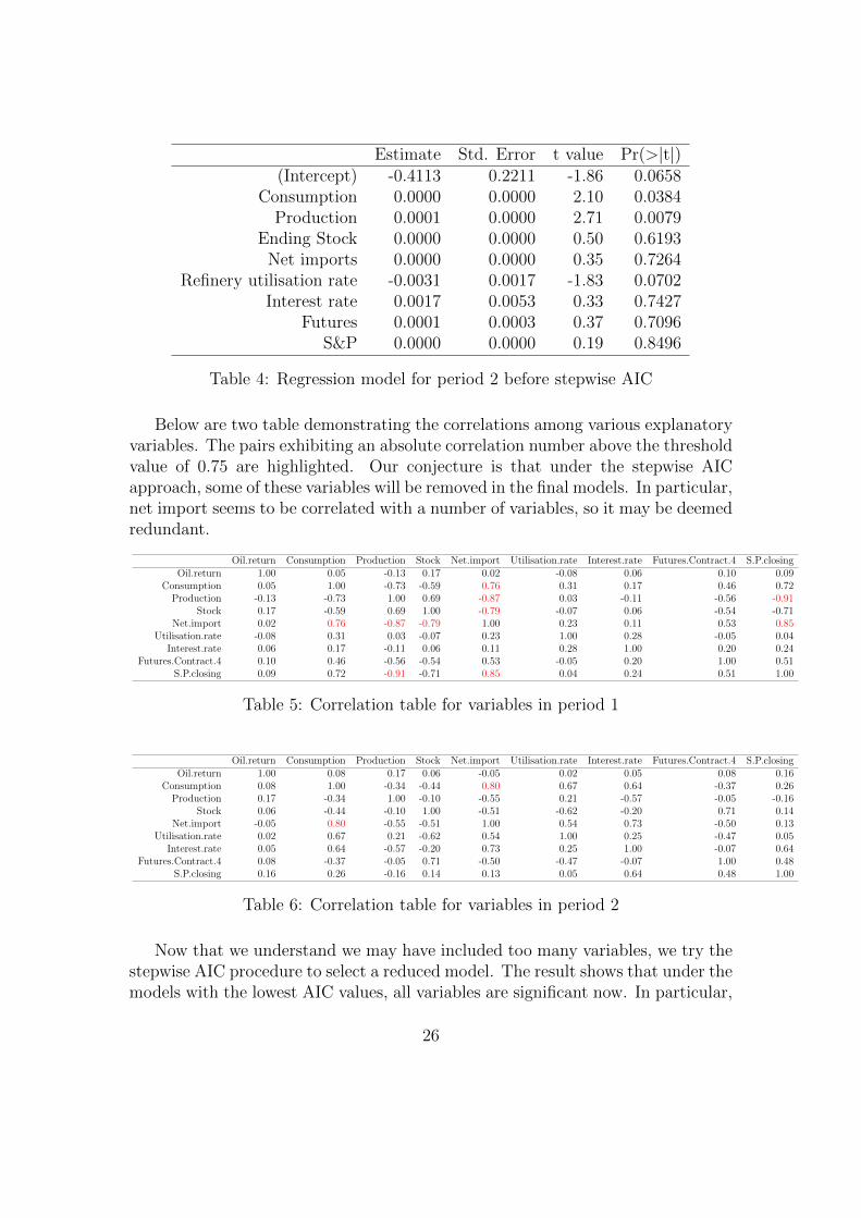
Table 4: Regression model for period 2 before stepwise AIC

Below are two table demonstrating the correlations among various explanatoryvariables. The pairs exhibiting an absolute correlation number above the thresholdvalue of 0.75 are highlighted. Our conjecture is that under the stepwise AICapproach, some of these variables will be removed in the final models. In particular,net import seems to be correlated with a number of variables, so it may be deemedredundant.

Oil.return Consumption Production Stock Net.import Utilisation.rate Interest.rate Futures.Contract.4 S.P.closingOil.return 1.00 0.05 -0.13 0.17 0.02 -0.08 0.06 0.10 0.09

Consumption 0.05 1.00 -0.73 -0.59 0.76 0.31 0.17 0.46 0.72Production -0.13 -0.73 1.00 0.69 -0.87 0.03 -0.11 -0.56 -0.91

Stock 0.17 -0.59 0.69 1.00 -0.79 -0.07 0.06 -0.54 -0.71Net.import 0.02 0.76 -0.87 -0.79 1.00 0.23 0.11 0.53 0.85

Utilisation.rate -0.08 0.31 0.03 -0.07 0.23 1.00 0.28 -0.05 0.04Interest.rate 0.06 0.17 -0.11 0.06 0.11 0.28 1.00 0.20 0.24

Futures.Contract.4 0.10 0.46 -0.56 -0.54 0.53 -0.05 0.20 1.00 0.51S.P.closing 0.09 0.72 -0.91 -0.71 0.85 0.04 0.24 0.51 1.00

Table 5: Correlation table for variables in period 1

Oil.return Consumption Production Stock Net.import Utilisation.rate Interest.rate Futures.Contract.4 S.P.closingOil.return 1.00 0.08 0.17 0.06 -0.05 0.02 0.05 0.08 0.16

Consumption 0.08 1.00 -0.34 -0.44 0.80 0.67 0.64 -0.37 0.26Production 0.17 -0.34 1.00 -0.10 -0.55 0.21 -0.57 -0.05 -0.16

Stock 0.06 -0.44 -0.10 1.00 -0.51 -0.62 -0.20 0.71 0.14Net.import -0.05 0.80 -0.55 -0.51 1.00 0.54 0.73 -0.50 0.13

Utilisation.rate 0.02 0.67 0.21 -0.62 0.54 1.00 0.25 -0.47 0.05Interest.rate 0.05 0.64 -0.57 -0.20 0.73 0.25 1.00 -0.07 0.64

Futures.Contract.4 0.08 -0.37 -0.05 0.71 -0.50 -0.47 -0.07 1.00 0.48S.P.closing 0.16 0.26 -0.16 0.14 0.13 0.05 0.64 0.48 1.00

Table 6: Correlation table for variables in period 2

Now that we understand we may have included too many variables, we try thestepwise AIC procedure to select a reduced model. The result shows that under themodels with the lowest AIC values, all variables are significant now. In particular,

26

net import is removed, as expected. Note also that the remaining variables do notexhibit multicollinearity anymore, as seen in the correlation tables. We thereforeconclude them as the final models.

Estimate Std. Error t value Pr(>|t|)(Intercept) -0.4470 0.1372 -3.26 0.0015Production -3.642e-05 0.0000 -3.21 0.0018

Ending stock 1.140e-06 0.0000 4.23 0.0001Interest rate 1.184e-03 0.0008 1.47 0.0145

Table 7: Regression model for period 1 after stepwise AIC


Consumption 5.890e-07 0.0000 2.94 0.0041Production 4.789e-05 0.0000 3.29 0.0014

Refinery utilisation rate -3.477e-03 0.0014 -2.47 0.0151

Table 8: Regression model for period 2 after stepwise AIC

5.2 Residual analysis

For both periods, we present a normal QQ plot and a plot of residuals against fittedvalues. The second plots for both periods look reasonaly scattered. The normalQQ plot in period 2 looks a bit off the line at the bottom left corner. A closerlook reveals that those points (refering to data points no. 67, 68 and 69) all evolvearound the financial crisis, where data of almost all variables experience abnormallylarge fluctuations. If we ignore these three points, the normality assumption ofresiduals is still valid. Hence, treating these points as outliers, we do not haveenough evidences to say the two models fitted violate the regression assumptionsmade before.

27

-2 -1 0 1 2

-2-1

01

23


Stand

ardize

d resi

duals

Normal Q-Q

85

72

69

-0.02 0.00 0.01 0.02

-0.05

0.00

0.05

Fitted valuesResiduals

Figure 17: Residual plots of linear model 1 in the first period

-2 -1 0 1 2

-3-2

-10

12

3


Stand

ardize

d resi

duals

Normal Q-Q

69

6768

-0.02 0.00 0.02

-0.10

-0.05

0.00

0.05

Fitted values

Residuals

Figure 18: Residual plots of linear model 2 in the second period

28

6 Conclusion

6.1 Forecasting comparison

Now that we have produced several feasible models, we aim to analyse their fore-casting accuracies. Here, we use a similar approach as in [15], where multiplen-step ahead (n=1,3,12 in this case) MSE and MAE are generated. This way, weget a better picture of how well these models predict the future as time evolves.The lowest value in each row has been highlighted in read, indicating it as the bestmodel in terms of forecasting power.

Period 1 (1M) Pure ARIMA(0,0,1) GARCH(1,1) APARCH(1,1) Regression

MSE 0.0008273015 1.508008e-06 3.151164e-05 0.03918434MAE 0.02793794 0.001228010 0.005613523 0.0271045


MSE 0.0003327995 0.0001827951 0.0001540007 0.1051161MAE 0.01497401 0.01352018 0.01240970 0.3240156

Period 1 (3M) ARIMA(2,0,2) GARCH(1,1) APARCH(1,1) Regression

MSE 0.0005606348 3.338360e-04 3.438372e-04 0.0008208638MAE 0.02127127 0.013742670 0.015204508 0.05710662


MSE 0.0019537375 0.0016644569 0.0016768143 0.02703593MAE 0.03824697 0.03653158 0.03638651 0.3506823

Period 1 (12M) ARIMA(2,0,2) GARCH(1,1) APARCH(1,1) Regression

MSE 0.0009523015 9.501257e-04 9.526260e-04 0.001311681MAE 0.02710461 0.026769001 0.027134460 0.0324022


MSE 0.0007042058 0.0007023213 0.0007060481 0.6945591MAE 0.02148884 0.02090367 0.02085000 0.8328744

Table 9: Comparison of forecast accuracy (1M, 3M and 12M ahead)

6.2 Concluding remarks

1. Univariate approach versus linear regression approach: The uni-variate GARCH and APARCH clearly outform the other two models, as theyalways produce the lowest MAE and MSE for all three forecasting periods.We note that the regression model is not as effective as the univariate ap-proach. This is in line with the results produced in [15], in which univariate

29

models, APARCH in particular, outperform the model with a list of explana-tory variables chosen based on economic intuitions. This suggests that thevariables included are not relevant enough to accurately drive oil prices.

2. APARCH versus GARCH: As for the two ARCH models we propose,APARCH is more accurate than GARCH in terms of reducing forecast er-rors in the second period and vice versa. This suggests APARCH is moreeffective in capturing assymetric volatility dynamics, which is the fact thatbear markets tend to spike up volatility more than bull markets, a phe-nomenon which is more obvious in period 2. Again, this is in line with themathematical feature of APARCH suggested in [8].

3. Period 1 versus period 2: In the second period, the market is evidentlyunder a more turbulent condition, especially during the financial crisis. Wecan evidently say that there is a structural change from period 1 to period 2.The linear regression model that is fitted provides less satisfactory residualplots. In particular, the normal distribution assumption of residuals looksless convincing, which suggests linear regression models fail to capture tailrisks or to respond effectively to tailed events.

4. Using GARCH/APARCH versus using pure ARIMA: We note thatvariance of log return in the second period amounts to 595.99, while that ofthe first period is only 31.58. Though we also see price fluctuations in the firstperiod, such scale is definitely larger in the second period, especially duringthe financial crisis where see a significant decline in oil prices from historicalhighs. In particular, this volatile period makes a significant contribution tothe much larger variance of the second period. Accordingly, this providesintuitive reasoning on why GARCH/APARCH is necessary in the secondperiod while a pure ARIMA model is sufficient for the first period.

30

7 R codes

library(TSA); library(MASS)

library(FitAR); library(tseries)

library(timeSeries); library(fGarch)

library(forecast); library(reporttools)

data<-read.csv(’~Oilfactors1.csv’, header=TRUE)

data

##Univariate approach##

plot(ts(data[,11][1:240],start=c(1993,3),frequency=12),

ylab="Monthly WTI spot price US$")

abline(v=2003)

#Divide it into two 10-year horizons

oilspot.ts1<-ts(data[,11][1:109],start=c(1993,3),frequency=12)

oilspot.ts2<-ts(data[,11][122:230],start=c(2003,3),frequency=12)

#Set up realised values for validation

realised.ts1<-diff(log(ts(data[,11][1:121],start=c(1993,3),frequency=12)))

realised.ts2<-diff(log(ts(data[,11][122:242],start=c(2003,3),frequency=12)))

realised.ts1; realised.ts2

oilspot.ts1;oilspot.ts2;

summary(oilspot.ts1); summary(oilspot.ts2);

head(oilspot.ts1);head(oilspot.ts2);

#BoxCox plots to show the need of log transformation

BoxCox.ts(oilspot.ts1); BoxCox.ts(oilspot.ts2);

plot(log(ts(data[,11][1:240],start=c(1993,3),frequency=12)),

ylab="Monthly WTI spot price US$"); abline(v=2003)

#ADF test indicating non-stationarity

adf.test(log(oilspot.ts1),alternative=c(’stationary’))

adf.test(log(oilspot.ts2),alternative=c(’stationary’))

#ADF test indicating non-stationarity

adf.test(diff(as.vector(log(oilspot.ts1))),alternative=c(’stationary’))

adf.test(diff(as.vector(log(oilspot.ts2))),alternative=c(’stationary’))

#log return plot

31

plot(diff(log(ts(data[,11][1:240],start=c(1993,3),frequency=12))),

ylab="Monthly WTI spot price US$")

abline(v=2003,h=0)

log.return1<-diff(log(oilspot.ts1))

log.return2<-diff(log(oilspot.ts2))

log.return1;log.return2

#ACF and PACF plots

par(mfrow=c(1,2));

acf(as.vector(log.return1),drop.lag.0=FALSE)

pacf(as.vector(log.return1))

acf(as.vector(log.return2),drop.lag.0=FALSE)

pacf(as.vector(log.return2))

#Write a function to compute AIC of various ARMA orders

AICfn<-function(N,K)

{

for(i in 1:N)

{for(j in 1:N)

{

print(AIC(arima(K,order=c(i-1,0,j-1))))

}}}

AICfn(3,log.return1)

AICfn(3,log.return2)

#Models determined

model1<-arima(log.return1,order=c(0,0,1),include.mean=FALSE)

model2<-arima(log.return2,order=c(2,0,2),include.mean=FALSE)

#Residual analysis

plot(model1$resid);abline(h=0)

plot(model2$resid);abline(h=0)

mean(model1$resid); mean(model2$resid)

#Residual ACF and PACF plots

acf(as.vector(model1$resid),drop.lag.0=FALSE)

pacf(as.vector(model1$resid))

acf(as.vector(model1$resid^2),drop.lag.0=FALSE)

32

pacf(as.vector(model1$resid)^2)

acf(as.vector(model2$resid),drop.lag.0=FALSE)

pacf(as.vector(model2$resid))

acf(as.vector(model2$resid^2),drop.lag.0=FALSE)

pacf(as.vector(model2$resid)^2)

#Normality tests

qqnorm(residuals(model1)); qqline(residuals(model1))

qqnorm(residuals(model2)); qqline(residuals(model2))

jarque.bera.test(model1$resid); jarque.bera.test(model2$resid)

#Independence tests

McLeod.Li.test(,model1$resid,gof.lag=20)

McLeod.Li.test(,model2$resid,gof.lag=20)

#Write a function to compute AICs of various GARCH orders

AICfn2<-function(N,K)

{

for(i in 1:(N+1))

{ for(j in 1:N)

{

print(AIC(garch(residuals(K),order=c(i,j-1),trace=FALSE)))

}}}

AICfn2(3,model1); AICfn2(3,model2)

#GARCH model fitted

model.garch2<-garch(model2$resid,order=c(1,1),trace=F)

model.garch2.res<-resid(model.garch2)[-1]

acf(model.garch2.res,drop.lag.0=FALSE)

pacf(model.garch2.res)

acf(model.garch2.res^2,drop.lag.0=FALSE)

pacf(model.garch2.res^2)

#For comparing forecast accuracy, fit GARCH/APARCH models

gfit1<-garchFit(formula=~arma(0,1)+garch(1,1),

data=log.return1,trace=FALSE,include.mean=FALSE)

gfit11<-garchFit(formula=~arma(0,1)+aparch(1,1),


gfit2<-garchFit(formula=~arma(2,2)+garch(1,1),

33


gfit22<-garchFit(formula=~arma(2,2)+aparch(1,1),


##Linear regression approach##

cor(data[,2:10][1:108,])

cor(data[,2:10][121:228,])

par(mfrow=c(2,8))

x11<-data[,c(3:10)][(1:108),]

x22<-data[,c(3:10)][(121:228),]

y1<-data[,2][(1:108)]

y2<-data[,2][(121:228)]

x1.ts<-ts(x11,start=c(1993,4),frequency=12)

x2.ts<-ts(x22,start=c(2003,4),frequency=12)

for (i in 1:8) {plot(x1.ts[,i],ylab=i); abline(v=2003)}

for (i in 1:8) {plot(x2.ts[,i],ylab=i); abline(v=2003)}

lm1<-lm(y1~x11[,1]+x11[,2]+x11[,3]+x11[,4]+x11[,5]+x11[,6]+x11[,7]+x11[,8])

lm2<-lm(y2~x22[,1]+x22[,2]+x22[,3]+x22[,4]+x22[,5]+x22[,6]+x22[,7]+x22[,8])

summary(lm1);summary(lm2);

#Carry stepwise AIC for model selection

new.lm1<-stepAIC(lm1); new.lm2<-stepAIC(lm2)

summary(new.lm1);

summary(new.lm2);

#No evidence of multicollinearity from correlation table

cor(x22[,c(2,3,7)][(1:108),])

cor(x11[,c(1,2,5)][(1:108),])

par(mfrow=c(1,2))

#Residual analysis, regression assumptions not violated

plot(new.lm1,c(2))

plot(new.lm2,c(2))

plot(fitted.values(new.lm1),new.lm1$residuals)

plot(fitted.values(new.lm2),new.lm2$residuals)

c<- as.vector(new.lm1$coefficients)

d<- as.vector(new.lm2$coefficients)

34

#Generate new matrix containing predicted values of variables

#1-month ahead for period 1

new.z1<-matrix(nrow=1,ncol=3)

new.z1[,1]<-as.vector(predict(x1.ts[,2],h=1)$mean)




new.k1<-matrix(nrow=1,ncol=3)

new.k1[,1]<-as.vector(predict(x2.ts[,1],h=1)$mean)























#Compute the forecast errors for regression approach

re.forecast.error11<-new.z%*%c[2:4]+c[1]-data[,2][109:109]

re.forecast.error21<-new.k%*%d[2:4]+d[1]-data[,2][229:229]


re.forecast.error23<-new.k%*%d[2:4]+d[1]-data[,2][229:231]


35

re.forecast.error212<--new.k%*%d[2:4]+d[1]-data[,2][229:240]

#Compute MSE and MAE

mean(abs(re.forecast.error11));mean(abs(re.forecast.error21))

mean(abs(re.forecast.error11)^2);mean(abs(re.forecast.error21)^2)





#Next, compute the forecast errors for univariate approach

forecast.error1<-vector(length=12); forecast.error2<-vector(length=12);



mse.forecast.error1<-vector(length=12); mse.forecast.error2<-vector(length=12);

mse.forecast.error11<-vector(length=12);




for(i in 1:12)

{forecast.error1[i]<-mean(abs(predict(gfit1,n.ahead=i)

$meanForecast-data[,2][109:(108+i)]));

forecast.error11[i]<-mean(abs(predict(gfit11,n.ahead=i)


forecast.error111[i]<-mean(abs(forecast(Arima(log.return1,

order=c(0,0,1),include.mean=FALSE),

h=12)$mean-data[,2][109:(108+i)]));}

for(i in 1:12)

{mse.forecast.error1[i]<-mean((predict(gfit1,n.ahead=i)

$meanForecast-data[,2][109:(108+i)])^2);

mse.forecast.error11[i]<-mean((predict(gfit11,n.ahead=i)


mse.forecast.error111[i]<-mean((forecast(Arima(log.return1,


h=12)$mean-data[,2][109:(108+i)])^2);}

for(i in 1:12)

36

{forecast.error2[i]<-mean(abs(predict(gfit2,n.ahead=i)


forecast.error22[i]<-mean(abs(predict(gfit22,n.ahead=i)


forecast.error222[i]<-mean(abs(forecast(Arima(log.return2,


h=12)$mean-data[,2][229:(228+i)]));}

for(i in 1:12)

{mse.forecast.error2[i]<-mean((predict(gfit2,n.ahead=i)


mse.forecast.error22[i]<-mean((predict(gfit22,n.ahead=i)


mse.forecast.error222[i]<-mean((forecast(Arima(log.return2,


h=12)$mean-data[,2][229:(228+i)])^2);}

#Compute MSE and MAE

mean(abs(forecast.error1)); mean(abs(forecast.error11));



mean((forecast.error1)^2); mean((forecast.error11)^2);

mean(abs(forecast.error111)^2); mean((forecast.error2)^2);

mean((forecast.error22)^2); mean(abs(forecast.error222)^2);

37

References

[1] G. Box and G. Jenkins, (1970) Time series analysis: Forecasting and control.San Francisco: Holden-Day

[2] P. Brockwell and R. Davis, (1991) Time Series: Theory and Methods. Springer-Verlag

[3] G. M. Ljung and G. Box (1978) On a Measure of a Lack of Fit in Time SeriesModels. Biometrika 65 (2): 297–303

[4] M. Arranz, (2005) Portmanteau Test Statistics in Time Series. Tol-Project.Org

[5] R. Engle, (1982) Autoregressive Conditional Heteroscedasticity with Estimatesof Variance of United Kingdom Inflation”. Econometrica 50:987-1008

[6] T. Bollerslev, (1986) Generalized Autoregressive Conditional Heteroskedastic-ity. Journal of Econometrics, 31:307-327

[7] R. Engle, (2001) GARCH 101: The Use of ARCH/GARCH Models in AppliedEconometrics. Journal of Economic Perspectives 15(4):157-168

[8] Ding, Z., C. W. J. Granger, and R. F. Engle (1993). A Long Memory Propertyof StockMarket Returns and a New Model,” Journal of Empirical Finance, 1,83-106.

[9] D.A. Dickey and W.A. Fuller (1979) Distribution of the estimators for autore-gressive time series with a unit root. J. Amer. Statist. Assoc., 74:427–431

[10] H. Akaike (1974) A new look at the statistical model identification. IEEETrans. Automat. Control, 19(6):716–72

[11] C. Jarque and A. Bera (1980) Efficient tests for normality, homoscedastic-ity and serial independence of regression residuals. Economics Letters 6 (3):255–259

[12] A. McLeod and W. K. Li, (1983) Diagnostic checking ARMA time series mod-els using squared residual autocorrelations. Journal of Time Series Analysis, 4,269273

[13] N. Meade and A. Cooper, (2007) An Analysis of Oil Price Behaviour. Quan-titative and Qualitative Analysis in Social Sciences Volume 1, Issue 2, 2007,33-54

38

[14] F. Bosler (2010) Models for Oil Price Prediction and Forecasting. San DiegoState University

[15] T. Gileva (2010) Econometrics of Crude Oil Markets. Universit´e Paris 1Panth´eon-Sorbonne

[16] C. Tsirimokos, (2011) Price and Income Elasticities of Crude Oil Demand, thecase of ten IEA countries. Swedish University of Agricultural Sciences, Facultyof Natural Resources and Agricultural Sciences, Master Degree Thesis No. 705,ISSN 1401-4084

[17] R. Pirog, (2005) World Oil Demand and its Effect on Oil Prices. CRS Reportfor Congress, order code RL32530

[18] E. Papapetrou, (2001) Oil Price Shocks, Stock Market, Economic Activityand Employment in Greece. Energy Economics, Vol. 23, pp. 511-532.

[19] Huang, B.N., M.J. Hwang, and Peng, H.P., (2005) The Asymmetry of theImpact of Oil Price Shocks on Economic Activities: An Application of theMultivariate Threshold Model. Energy Economics, Vol. 27, pp. 455-476.

[20] Cunado J. and de Gracia F., (2005) Oil prices, economic activity and inflation:evidence for some Asian countries. Energy Economics, Vol. 45, pp. 65–83.

[21] Guo, H. and. Kliesen, K (2005). ‘Oil Price Volatility and U.S. MacroeconomicActivity’, Federal Reserve Bank of St. Luis, Review, Vol. 87, No.6, pp. 669-683.

[22] Lehmann, E. L. and Casella, G. (1998) Theory of Point Estimation (2nd ed.).New York: Springer. ISBN 0-387-98502-6. MR 1639875.

[23] Huang, R.D., Masulis, R.W. and Stoll, H.R. (1996) Energy shocks and finan-cial markets. Journal of Futures Markets, 16, 3956.

[24] Kaufmann, R.K., Dees, S., Karadeloglou and P., Sanchez, M. (2004) DoesOPEC matter? An econometric analysis of oil prices. The Energy Journal,25(4), 67-90.

[25] Pindyck, R. S., (2004) Volatility and Commodity Price Dynamics. Journal ofFutures Markets 24, 1029–1047.

[26] A. Deng, K. King and D. Metz (2012) An Econometric Analysis of Oil PriceMovements: The Role of Political Events and Economic News, Financial Trad-ing, and Market Fundamentals. Bates White Economic Consulting

[27] X. Mu and H. Ye (2010) Understanding the Crude Oil Price: How Importantis the China Factor. USAEE-IAEE WP 10-050

39

Time Series Modelling of Monthly WTI Crude Oil Returns

Documents

Transcript of Time Series Modelling of Monthly WTI Crude Oil Returns