1

School of Economics and Management

NEKP01 Master’s Thesis 2015-08-19

Measuring Risk for WTI Crude Oil An application of Parametric Expected Shortfall

Author: Supervisor:

Alexander Eriksson Birger Nilsson

2015-08-19

2

Abstract

Oil is the most traded commodity in the world and is an important part in the global

economy. The change in the price of oil has an effect on all sectors of the economy, and

the ability to capture its risk is an important research topic. This study calculates the

risk of one benchmark crude oil (West Texas Intermediate) over the period 1986-2015

by estimating the Value-at-Risk (VaR) and the Expected Shortfall (ES) on daily spot

returns. More specifically, this is done by using a GARCH (1, 1) model with the normal

distribution, the t-distribution, and the Generalized Error Distribution (GED). The study

uses a rolling window to estimate these risk measurements creating 7125 estimates for

each distribution in each tail. The normal distribution was the worst performing

distribution on both ES and VaR according to the backtests. The t-distribution

performed good ES estimates; however it was not as accurate when calculating VaR. The

GED performed the best when calculating VaR but constantly underestimated ES. The

main conclusion is that both GED and the t-distribution are needed when estimating the

risk for WTI.

Keywords: Risk, Expected shortfall, VaR, Backtesting, Crude oil

3

Table of content

List of Graphs ..................................................................................................................................... 4

List of Tables ...................................................................................................................................... 4

List of Abbreviations ......................................................................................................................... 5

1. Introduction ................................................................................................................................... 6

1.1 Background ............................................................................................................................ 6

1.2 Risk measurements ..................................................................................................................... 7

1.2.1 Value-at-Risk ........................................................................................................................ 7

1.2.2 Expected Shortfall ............................................................................................................... 9

1.3 Literature review ....................................................................................................................... 10

1.4 Objective ..................................................................................................................................... 12

1.4.2 Delimitations ....................................................................................................................... 12

2 Methods ............................................................................................................................................. 13

2.1 Parametric estimation of the Risk measurements .................................................................. 13

2.1.1 GARCH ................................................................................................................................. 14

2.2 Backtesting the risk measurements ......................................................................................... 18

2.2.1 Backtesting VaR .................................................................................................................. 18

2.2.2 Backtesting Expected Shortfall .......................................................................................... 21

2.2.3 General discussion of the Backtesting methods. .............................................................. 28

3 Data .................................................................................................................................................... 30

4 Results ............................................................................................................................................... 32

5 Further research ............................................................................................................................... 34

6 Conclusion ......................................................................................................................................... 34

7 References ......................................................................................................................................... 35

4

List of Graphs Graph 1: Illustration of parametric VaR. .................................................................................................................. 8

Graph 2: Comparison of VaR and ES .......................................................................................................................... 9

Graph 3: Probability Density Function of the t-distribution. ........................................................................ 16

Graph 4: Probability Density Function of the GED ............................................................................................ 17

Graph 5: Daily returns ................................................................................................................................................... 30

Graph 6: The evolution of prices............................................................................................................................... 30

List of Tables Table 1: Descriptive statistics .................................................................................................................................... 31

Table 2: VaR backtesting results ............................................................................................................................... 32

Table 3: ES backtesting results .................................................................................................................................. 32

5

List of Abbreviations

CC Conditional Coverage

DOF Degree of Freedom

ES Expected Shortfall

GED Generalized Error Distribution

LR Likelihood Ratio

PDF Probability Density Function

UC Unconditional Coverage

VaR Value-at-Risk

WTI West Texas Intermediate

6

1. Introduction

1.1 Background

Oil is the most traded commodity in the world and forty percent of the world’s energy

originates from crude oil. 1 There are numerous types of crude oils, and these are priced

in relationship to the two main crude oil benchmarks that sets the world price of oil.

Specifically, the West Texas Intermediate (WTI), which is the US benchmark, and the

Brent crude, which is the European Benchmark.2 The spot price of these benchmark are

immensely important since: “The prices of these benchmarks are used by oil companies

and traders to price cargoes under long-term contracts or in spot market transactions;

by futures exchanges for the settlement of their financial contracts; by banks and

companies for the settlement of derivative instruments such as swap contracts; and by

governments for taxation purposes.”3 The price of the benchmarks has been notoriously

volatile since the collapse of the OPEC pricing system, and the increased competition and

deregulation since the 1980’s.4 These high fluctuations in price are driven by political

events, such as the Iraqi invasion of Kuwait, when the price almost doubled in response

to the invasion, but also by the business cycle that drives supply and demand

imbalances.5 The price of oil can have an important effect on government finances in oil

producing countries, since the budget is balanced for a certain oil price, and any

deviation from this price could lead to large deficits or surpluses.6 The risks in these

benchmarks are of great interest because of the impact the price has on both the public

and private sector in the world economy.7 The high volatility of oil prices and the

increased focus on risk management in recent years are the reasons for this study. The

study will therefore estimate the risk of oil prices using methods in the forefront of

today’s research. Next section will explore the different risk measurement tools most

used to estimate the risk of an asset, which will be followed by a literature review and

the outline of the objective of this study.

1 International Energy Agency (2014) Key World Energy STATISTICS [Online]. Available: http://www.iea.org/publications/freepublications/publication/KeyWorld2014.pdf [Accessed 12 May 2015] 2 Edwards, Davis W. "Energy Trading and Investing." (2010) p. 142 3 Fattouh, Bassam. An anatomy of the crude oil pricing system. Oxford, England: Oxford Institute for Energy Studies, 2011 p. 24 4 Ibid p. 6 5 Giot Pierre, and Sébastien Laurent. "Market risk in commodity markets: a VaR approach." Energy Economics 25.5 (2003): p. 435-457. p. 437 6 Farzanegan, Mohammad Reza, and Gunther Markwardt. "The effects of oil price shocks on the Iranian economy." Energy Economics 31.1 (2009): 134-151. 7 Kilian, Lutz. "The economic effects of energy price shocks." (2007).

7

1.2 Risk measurements

There has been an increased focus on risk management in the last 20 years. An

expansion of the financial markets and derivative trading, along with an extensive list of

companies suffering financial disaster because of improper risk management have

spurred the development of better risk management practices.8 The next section will

explain the most widespread methods for calculating the risk on asset returns.

1.2.1 Value-at-Risk 9

The most commonly used market risk measurement tool is the Value-at-Risk (VaR). This

measurement was introduced by Morgan Stanley in the document Riskmetrics in 1994,

and was adopted by the Basel accord to be used by regulators to calculate the capital

requirements of banks.10 The study has the point of view of two companies where one

has a long position, and the other has a short position, on a portfolio of one barrel of oil.

The risk is therefore the relative price changes of this barrel, i.e. the arithmetic returns

according to the following formula: 𝑅𝑡 = 100 ∗ ( 𝑃𝑡−𝑃𝑡−1

𝑃𝑡−1). Since this risk measure is

focused on the distribution of returns, VaRα is defined as the largest return, such that the

probability of observing a return less than this is equal to 1-α, equation 1.11

𝑉𝑎𝑅𝛼 = Pr(𝑅 ≤ −𝑉𝑎𝑅∝) ≤ 1 − 𝛼12 (1)

The VaRα can therefore be seen as the α-quantile of the return distribution. Which

position is taken dictates which tail under the return distribution is considered the risk,

a short position, the right tail, while a long position the left tail of the return distribution.

On a long position an asset with a correctly estimated VaR will suffer a negative return

greater than –VaR, a so-called VaR violation, with a probability of 1-α over the holding

period.13 Common choices for α is 99% and 95% meaning that a VaR violation will occur

on average once every 100 days for α=99%, and five times per 100 days for α=95%.

The 99% VaR for an asset for which the returns are normally distributed, with variance

one and mean zero is 2.326. Therefore a negative return greater than -2.326% will occur

8 Dowd, Kevin. Measuring market risk. John Wiley & Sons, 2005. p. 1-4 9 Ibid p. 30 10 Chen, James Ming. "Measuring Market Risk Under the Basel Accords: VaR, Stressed VaR, and Expected Shortfall." Stressed VaR, and Expected Shortfall (March 19, 2014) 8 (2014): 184-201. 11 Nilsson, Birger( 2014) “Value-at risk” lecture notes in. NEKN83/TEK180 spring 2014. Lund University p. 2 12 Nilsson, Birger( 2014) “Value-at- risk” p. 2 13 The holding period determines how far in the future the VaR estimates are calculated for. The VaR for holding periods over one

day the calculations are as follows,√𝐻𝑜𝑙𝑑𝑖𝑛𝑔𝑝𝑒𝑟𝑖𝑜𝑑 ∗ 𝑉𝑎𝑅. For regulatory purposes it is 10 days, however in this study the holding

period is one day, and will therefore be omitted in all formulas.

8

on average once every 100 days, meaning that the area to the left of -2.326 under the

probability density function is 0.01=1-α. (Graph 1)

Graph 1: Illustration of parametric VaR, created in R.

The advantages of VaR are that it is easily understood and intuitive, as it is probabilistic

(i.e. the company will suffer a return loss greater than Y with probability X). Other

attractive properties of VaR are that it is common consistent measurement over

different positions as it can be applied to almost all types of portfolios, whether it is

equity or a currency portfolio, as well as its ability to aggregate the risk of different sub

positions.14 These attractive properties are the reasons why VaR is so widely adopted by

regulators and companies alike.15 However, there are several disadvantages to VaR

which are not to be underestimated.

VaR does not reveal anything about the size of the return loss given that a VaR violation

has occurred, a so-called tail event.16 This drawback is not negligible as two different

assets with similar VaR estimate can have different risk properties, as its behaviors in

the tails are not taken into consideration when estimating VaR. Also, if traders in a

company are limited to how much VaR their positions can have it could incentivize them

to take positions that are not beneficial to their employer. By taking positions that suffer

small losses unless a tail event occurs, at which point a very large loss occurs, the trader

can take a riskier position than the company wants the trader to take.17Another major

drawback of VaR is that it is not a subadditive risk measurement. This means that this

risk measure does not encourage diversification as two assets separately can produce a

lower VaR estimate than a portfolio of them combined. “The failure of VaR to be

subadditive is a fundamental problem because it means that VaR has no claim to be

regarded as a ‘proper’ risk measure at all. A VaR is merely a quantile. It has uses as a

14 Dowd 2005 p. 12 15Ibid p. 13 16 Ibid p. 13 17 Ibid p. 14

9

quantile, but is very unsatisfactory as a risk measurement.”18 Due to the drawbacks of

VaR the measurement expected shortfall (ES) is proposed

1.2.2 Expected Shortfall 19 20

Expected shortfall (ES) measures the size of the return given a tail event, i.e. it is the

expected return given a VaR violation. ES is therefore subordinate VaR, since the VaR

computations need to be performed first in order to calculate ES. By definition, ES will

always be greater than VaR. Equation 2 below provides the mathematical definition of

Expected Shortfall in the continuous case, where 𝑓(R) is the probability density function

of the returns.

−𝐸𝑆∝,𝑡(𝑅) =1

1−∝∫ 𝑅 ∗ 𝑓(𝑅)𝑑𝑅

𝑉𝑎𝑅∝,𝑡(𝑅)

−∞ (2)

Graph 2: Comparison of VaR and ES

ES measures the expected returns when a tail event occurs, and therefore reveals what

is to be expected in a bad state.21 Following the case of normally distributed returns with

mean 0 and variance 1, the expected negative return is -2.667% given that the loss is

greater than -2.328%. In addition to providing information on the tail behavior to the

risk managers, ES is also considered to be an improved measurement compared to VaR

since it is always subadditive. Two assets in a portfolio will produce equal or lower ES

estimates compared to calculating ES on the assets separately, and thereby encouraging

diversification in the portfolio. ES also makes it more difficult for traders to take

positions that are not beneficial to the company since it is harder to “optimize” in the

way explained earlier, as the tail behavior of the returns is taken into consideration. For

18 Dowd 2005 p. 34 19 Dowd p. 34 20 Other names for ES are Expected Tail Loss(ETL), Conditional Value at Risk (CVaR) , and Average Value at Risk (AVaR). 21 Dowd 2005 p. 34

10

all the reasons above, ES is generally considered to be a superior risk measurement

compared to VaR. 22

While ES is considered to be a better risk measurement than VaR, the financial

regulations have been slow to switch from VaR to ES. One of the main reasons for this is

that there is no consensus on which method is best used to backtest the ES estimates.23

Some say ES is not even possible to backtest since is it does not have the property of

elicitability,24 this is however disputed. 25 26 Nevertheless, the literature provides some

backtesting procedures which make it possible to test the ES estimates.

1.3 Literature review

The objective of this section is to give an overview of the results of the existing literature

regarding parametric estimations for both ES and VaR on WTI crude oil. This will form

the basis for the objective of the study.

Chen and Hung calculated one day ahead conditional VaR on WTI spot returns using

rolling window estimation on daily data from January 2002 to March 2009.27 The

GARCH (1, 1) with normal distribution performed worse than the GED and t-distribution

over the out of sample period from January 2003 to March 2009. At a 99% confidence,

level the GED and the t-distribution performed equally well. Fan et al. estimated in

sample VaR using various GARCH with the normal distribution and GED, for daily

logarithmic WTI spot returns over the period from May 1987 to August 2005. 28 GARCH

(1, 1) performed better compared to any other number of lags for the normal GARCH

model, but the TGARCH model performed slightly better results than the GARCH. The

results indicate that negative shocks have more effect on the volatility than positive

ones. They also concluded that WTI price returns have excess kurtosis, also known as fat

tail properties, and that GED performed better than the normal distribution at the 99%

22

Dowd 2005 pp. 35 23

Acerbi, Carlo, and Balazs Szekely. "Back-testing expected shortfall." Risk 27.11 (2014). p. 2 24). Chen, James Ming. "Measuring Market Risk Under the Basel Accords: VaR, Stressed VaR, and Expected Shortfall." Stressed VaR,

and Expected Shortfall (March 19, 2014) 8 (2014): 184-201. p. 197

25 Acerbi and Szekely 2014 p. 2

26 A discussion of elicitability is outside the scope of this thesis. The interested reader can refer to the sources cited.

27 Cheng, Wan-Hsiu, and Jui-Cheng Hung. "Skewness and leptokurtosis in GARCH-typed VaR estimation of petroleum and metal asset

returns." Journal of Empirical Finance 18.1 (2011): 160-173 28

Fan, Ying, et al. "Estimating ‘Value at Risk’of crude oil price and its spillover effect using the GED-GARCH approach." Energy Economics 30.6 (2008): 3156-3171

11

level in both tails. The normal distribution consistently underestimated the risk. On a

95% level both distributions performed well and no statistical difference was

discovered.29 This is in complete contradiction to Xiliang and Xi. They found that GARCH

with GED is the best model for calculating VaR on logarithmic returns at a 95%

confidence level. In addition they found that GARCH with normal distribution performed

best at a 99% confidence level. This result was obtained by applying a rolling window

estimation over the out sample period from October 2004 to November 2008.30

Hung, Lee, and Liu estimated VaR for one-day-ahead logarithmic WTI spot price returns

using GARCH with the heavy-tailed distribution, normal distribution and t-distribution.

31 The study used observations from November 1996 to September 2006 of which the

last 500 observations are the out of sample period. Applying a rolling window to

calculate VaR, GARCH with the t-distribution and the normal distribution performed

poorly at low confidence intervals while at high they performed well. The heavy tail

distribution was the most accurate and most efficient measure at all confidence intervals

except for α≥99%, where it was not statistically different from the normal and t-

distribution.

Almli and Rege used data from July 1996 to April 2011 to estimate ES and VaR for WTI.

32 Their estimations were done by applying a rolling window to forecast the one day

ahead risk measure on the last 500 observations for both a long, and short position on

futures data. They concluded that the normal distribution was the worst performing

distribution for the GARCH VaR estimate while the t-distribution performed better. The

GED was neither best nor worst, and absolute best performing distribution was the

skewed t-distribution. When estimating ES, the normal distribution produced more

accurate results compared to the t-distribution and GED, which both consistently

overestimated the risk.

29 Fan et al. 2008 30

Xiliang, Zhao, and Zhu Xi. "Estimation of Value-at-Risk for Energy Commodities via CAViaR Model." Cutting-Edge Research Topics on Multiple Criteria Decision Making. Springer Berlin Heidelberg, 2009. 429-437 31

Hung, Jui-Cheng, Ming-Chih Lee, and Hung-Chun Liu. "Estimation of value-at-risk for energy commodities via fat-tailed GARCH

models." Energy Economics 30.3 (2008): 1173-1191 32 Almli, Eldar Nikolai, and Torstein Rege. "Risk Modelling in Energy Markets: A Value at Risk and Expected Shortfall Approach."

(2011).

12

Aloui and Marouk estimated the one day ahead VaR and ES on WTI spot using data from

January 1986 to March 2007, and concluded that WTI does not follow a normal

distribution, as the series have excess kurtosis and is asymmetric to the left. 33 The result

showed that a skewed t-distribution performed better compared to a symmetric t-

distribution.

When reviewing previous literature some questions emerge. Which distribution

produces the best estimates for conditional VaR and ES estimates? What role if any, does

the backtesting procedure have when evaluating the ES estimates? These questions lead

to the objective of this study.

1.4 Objective

The objective of this study is to answer the two following questions.

(i) When calculating parametric 99% 1-day ahead ES on WTI returns, what

distribution is superior?

(ii) Is the best distribution for estimating ES also the best for estimating VaR?

Given the previous research the expectation of the results are as follows:

E(i): The fat tailed distributions will be better at estimating ES compared to the normal

distribution, and the GED will be superior to the t-distribution.

E(ii): The same distribution that provides the best VaR estimate will also provide the

best ES estimate.

By evaluating (i) and (ii) over the period 1986-12-15 to 2015-03-25, this study hopes to

contribute to the literature with a greater understanding about the risk quantifications

of WTI spot prices. This is done by applying several backtesting methods on the ES

estimates, and thereby providing more robust results compared to previous literature.

1.4.2 Delimitations

This study excludes risk measurement estimation methods that depend on the extreme

value theorem as well as methods depending only on historical data without any

parametric assumptions, so-called non-parametric methods. This is done to focus solely

33 Aloui, Chaker, and Samir Mabrouk. "Value-at-risk estimations of energy commodities via long-memory, asymmetry and fat-tailed

GARCH models." Energy Policy 38.5 (2010): 2326-2339.

13

on conditional parametric estimations of VaR and ES. Another reason for this is that

some of the backtesting procedures that will be used need some distributional

assumptions which made the focus on parametric estimations natural. In order to

calculate the conditional parametric volatility, a normal symmetric GARCH (1, 1) is used

with symmetric distributions. The reason to only include GARCH (1, 1) is that it is a

fairly simple model that has been proven to perform well when trying to capture

volatility processes.34 This study furthermore excludes asymmetric distributions. If a

model is rejected in one tail but not rejected in the other, this would indicate that the

distributions of returns are asymmetric. Only the confidence level of 99% will be used,

both on long and short positions due to the interest in this study lie in the ability of the

distributions to capture extreme events in both tails.

2 Methods

This section will present a description of the methods used. First the method used to

estimate the risk measurements is presented, followed by the backtesting procedures

used to evaluate these estimates. The section will conclude with a general discussion of

the methodology.

2.1 Parametric estimation of the Risk measurements

Parametric estimation of a risk measurement is done by fitting a probability distribution

over the data. While it can be a powerful technique since the user has information

inferred from the distribution function, it is also a risky one because if an incorrect

distribution is used, the estimates produced can be completely inaccurate.35

There are two main ways of performing distribution fitting, unconditional and

conditional. The unconditional fitting does not depend on any conditional factors, and is

often applied on longer holding periods. Unconditional fitting will overestimate the risk

during calm periods, and more importantly, underestimate during volatile periods. In

contrast fitting a distribution conditional on an assumed volatility process will account

for calm and volatile periods. Conditional fitting is usually applied on shorter holding

34 Hansen, Peter R., and Asger Lunde. "A forecast comparison of volatility models: does anything beat a GARCH (1, 1)." Journal of applied econometrics” 20.7 (2005): 873-889. 35 Dowd 2005 p. 151

14

periods. 36 As the holding period in this study is one day, only conditional fitting will be

applied to estimate the volatility.

2.1.1 GARCH37

The most commonly used model when calculating conditional volatility is the GARCH (1,

1) model.38 This model is presented in equation 4 below. The GARCH accounts for

volatility clustering because the conditional volatility is based on previous error terms

and volatilities. If there is high variance at t, the GARCH model will predict high variance

at t+1. Therefore, the variance is not constant in the sample, and the model can account

for volatility clustering. The model is also symmetric, meaning that negative and positive

shocks have the same effect on volatility.

σt2 = ω𝑡 + α1,tϵt−1

2 +β1,tσt−12 (4)

β measures the persistence of the shocks on volatility while α measures the impact new

shocks have on the volatility. This model is crucial in this study as it will be used to

forecast the volatility for all the risk measurement. The volatility at t will be used to

forecast the volatility for t+1 as detailed in equation 5 below.39

σ̂t+12 = ω𝑡 + α1,tεt

2+β1,tσt2 (5)

There are two parts to a univariate time series, the variance equation, which in this case

is the GARCH model, and the mean equation. The mean equation in this study will be set

to zero since it is assumed that in a one day ahead forecast on returns the effect of the

mean equation will be negligible. In addition to the mean and variance equation,

parametric assumptions need to be made about the error terms. This is due to the fact

that the GARCH model is estimated by maximum likelihood, and a requirement for using

this method is that distributional assumption about the errors terms have to be made.40

In this study, as stated before, three such distributions will be used, the normal

distribution, the t-distribution and the Generalized Error Distribution (GED).

36 Dowd 2005 p. 152 37 Reider, Rob. "Volatility forecasting I: GARCH models." New York (2009). 38 Hansen and Lunde 2005 39 Reider 2009 40 Bollerslev, Tim. "A conditionally heteroskedastic time series model for speculative prices and rates of return." The review of economics and statistics (1987): 542-547.

15

For the GARCH estimates in this study, a rolling in-sample window of 250 observations

will be used to forecast the risk measurement for one day ahead. This implies that the

GARCH parameters are continuously re-estimated over the out of sample period from

1987-12-02 to 2015-03-24, leading to 7125 GARCH estimations. This is done because of

the long out of sample window since it is probable that the magnitudes of the

parameters in the GARCH model are not constant over the whole sample.

2.1.2 Normal Distribution41

The normal distribution or Gaussian distribution is an extremely commonly used

distribution, which exhibits many nice properties when performing statistical tests. One

of these is that the whole distribution is explained exclusively by two parameters; the

mean and variance as seen in in the PDF (Probability Density Function) below.42. Also,

the calculations for VaR are simple as can be seen in equation 6

VaRα(R𝑡+1) = σ̂t+1Zα, (6)

𝑓(𝑅) =1

√2𝜋𝜎2𝑒𝑥𝑝 {

−1

2

(𝑅 − �̅�)2

𝜎2 } 43

The normal distribution does not account for excess kurtosis, which is often present in

financial returns.44 When using a GARCH model, even the normal distribution can to a

limited extent account for excess kurtosis since the distribution is conditionally

normal.45 Nevertheless, it is a reasonable idea to include two distributions which will

produce even fatter tails, since they follow a conditional distribution with excess

kurtosis.

2.1.3 The t-distribution 46

The t-distribution usually referred to as student’s t-distribution, is a commonly used

distribution when performing calculations on financial data.47 This distribution is closely

linked to the normal distribution, but can account for fatter tails as seen in graph 3. The

shape of the distribution is dependent on three parameters, the mean, variance and the

41 Verbeek, Marno. A guide to modern econometrics. John Wiley & Sons, 2008. p 457. 42 Ibid p.457 43 Ibid p.457 44 Cont, Rama. "Empirical properties of asset returns: stylized facts and statistical issues." (2001): 223-236. 45 Dowd 2005 p 132 46 Hamilton, James Douglas. Time series analysis. Vol. 2. Princeton: Princeton university press, 1994 47 Dowd 2005 p. 159

16

Degrees of Freedom (DoF). Specifically, a lower value of DoF means that the distribution

has fatter tails, while a higher DoF means that the distribution will approach the normal

distribution. The normal distribution is therefore a special case of the t-distribution

when DOF, or v as defined in the probability density function below, approaches

infinity.48

The calculations for VaR is a little different compared to the normal distribution as seen

in equation 7.

Graph 3: Probability Density Function of the t-distribution at different Degrees of Freedom.

VaRα(R𝑡+1) = √𝑣−2

𝑣σ̂t+1Tα,v 49 (7)

𝑓𝑣(𝑅) =𝛤[𝑣 + 1 2⁄ ]

𝜎√(𝑣 − 2)𝜋𝛤(𝑣 2)⁄[1 +

1

𝑣 − 2(𝑅 − �̅�

𝜎)

2

]

−(𝑣+1) 2⁄

𝑓𝑜𝑟 𝑣 > 2, 𝑅 ∈ (−∞,∞)50

The critical value Tα,v is dependent on both the critical value α and on the DoF

parameter. Thereby the critical value is not fixed as in the case for the normal

distribution.

48 Hamilton 1994 49 Dowd 2005 p 159 50 Hamilton 1994

17

2.1.4 GED51

The Generalized Error Distribution, also known as Generalized Normal Distribution, or

exponential power distribution, similar to the t-distribution, can account for excess

kurtosis. The normal distribution is also a special case of the GED when the shape

parameter v=2. The shape of the curve at different values of the shape parameter can be

seen in graph 4.

Graph 4: Probability Density Function of the GED at different values of the shape parameter values.

𝑓𝑣(𝑅) =𝑣∗exp (

12 [𝑅 𝜆⁄ ]𝑣)

𝜆∗2[𝑣+1 𝑣⁄ ]𝛤(1 𝑣)⁄ 𝑓𝑜𝑟 (0 ≤ 𝑣 ≤ ∞),𝑅 ∈ (−∞,∞) 52

𝜆 = [ 2(−1 𝑘)⁄ 𝛤(1 𝑣)⁄

𝛤(3 𝑣)⁄]

1 2⁄

As seen in the graph 4 above this is the most complex of the three distributions used. It

is also the most uncommon. However, as mentioned earlier this distribution has

produced good results in previous studies. Now that the estimation techniques are

established for the risk measurements, the techniques of backtesting the estimates are

presented.

51

Vasudeva, R., and J. Vasantha Kumari. "On general error distributions." 2013 52 Ibid

18

2.2 Backtesting the risk measurements

In this section a summation of the methods used to backtest the VaR and ES estimates

are presented, which is followed by a brief discussion about their properties.

2.2.1 Backtesting VaR53

The Christoffersen test is the most widely adopted method for backtesting VaR.54 The

test is divided into two parts, the unconditional part, which examines if there is correct

number of VaR violations over the estimation period, and the conditional part which

tests if the violations are randomly distributed in the sample.

The unconditional part of the Christoffersen test checks if VaR violations, or days that

the VaR estimate is lower than the actual loss, follows a Bernoulli distribution with the

null hypothesis expressed in equation 8.55

𝐻0: 𝑉𝑡+1~ 𝑖. 𝑖. 𝑑 𝐵𝑒𝑟𝑛𝑜𝑢𝑙𝑙𝑖(1 − 𝛼) (8)

The α is the chosen confidence level, and in this study α =0.99. This means that the

expectation under the null hypothesis is that there is a violation on any given day with a

probability of 0.01. To check if the observed number of actual violations in the sample is

equal to the expected number of violations, the Christoffersen test uses the log

likelihood ratio test (LR). In order to perform this test, both the unconstrained and a

constrained value of the likelihood function are needed. The constrained part is defined

as L(1 − 𝛼) = (𝛼)t0(1 − 𝛼)t1 , where (1-α) is the probability of a violation under the null,

in our case 0.01. t0 is number of observed non-violations and t1 is number of observed

violations in the sample. The unconstrained model is L(π̂) = (1 − π̂)t0π̂t1 where t0 and t1

is the same as in the constrained model, but π̂ it is the actual probability of a violation as

observed in the series, π̂ = t1 (t0 + t1)⁄ . These two are used in the likelihood ratio test

equation 9.56

𝐿𝑅𝑢𝑐 = −2 𝑙𝑛[𝐿(1 − 𝛼) 𝐿(�̂�)⁄ ]~χ2(1) (9)

53 Christoffersen, Peter. "Backtesting." Encyclopedia of Quantitative Finance (2009). 54 Ibid 55 Ibid 56 Ibid

19

H0: (1-α)=�̂�

H1: (1-α) ≠ �̂�

If H0 is rejected, the VaR estimates have produced an incorrect number of violations in

the sample. Therefore the chosen model to estimate VaR does not accurately capture the

risk of the asset. 57

The conditional component of the Christoffersen test checks if the probability of a

violation at t+1 is p, conditional on what is known at t. The test examines if the

violations are independently distributed over the sample period. Violations that are

clustered indicate that there is an increased likelihood of a violation occurring in the

next period. A model that fails the conditional coverage Christoffersen test is not ideal

since the model does not accurately capture volatility clustering effects.58

The conditional part of the Christoffersen test, similar to the unconditional part, uses a

likelihood ratio test. To create the unrestricted part, a transition matrix as described in

equation 10 is needed. This matrix is used to calculate probability of a transition from

one state to another. �̂�01 is the probability of observing a non-violation followed by a

violation in the sample. This means that transition probabilities based on the VaR

violations given in the sample must be calculated. These estimates are then used as

described in equation 11 which is the unconstrained part of the LR test.59

∏1 = [1 − �̂�01 �̂�01

1 − �̂�11 �̂�11] (10)

𝐿(∏1) = (1 − �̂�01)𝑡00�̂�01

𝑡01(1 − �̂�11)𝑡10 �̂�11

𝑡11 (11)

The observed transitions in the sample are t, meaning that t01 is number of observations

that have a non-violation followed by a violation in the sample. In order to solve for the

actual probabilities in the transition matrix, the first derivatives with respect to π̂01 and

57

Christoffersen 2009 58 Ibid 59 Ibid

20

π̂11 in equation 11 are taken to produce the following formula used in the transition

matrix.60

�̂�01 =𝑡01

𝑡00 + 𝑡01, �̂�11 =

𝑡11

𝑡10 + 𝑡11

From this it is now possible to calculate the unconstrained part of the test. The

constrained model in the conditional part is the same as the unconstrained model in the

unconditional test.61

𝐿(�̂�) = (1 − �̂�)𝑡0�̂�𝑡1 (12)

Equation 11 and equation 12 are then combined to create the LR test, equation 13.62

𝐿𝑅𝑖𝑛𝑑𝑒𝑝 = −2 𝑙𝑛[𝐿(�̂�) 𝐿(∏1)⁄ ]~ 𝜒2(1) (13)

H0: �̂�01 = �̂�11

H1: �̂�01 ≠ �̂�11

The null hypothesis means that the information at t does not provide any information

about the probability of violation at t+1. Equation 9 and equation 13 are then combined

to the Christoffersen combined test equation 14 to test the overall validity of the model.

LRcc=LRuc+LRIND ~ 𝜒2(2) (14)

The Christoffersen test has two main parts LRuc, and LRcc, and if any of the null

hypotheses are rejected in either of the tests, the model used to calculate these VaR

estimates is not correct. While other backtesting methods for VaR exist, the

Christoffersen test has proven to perform well and therefore other tests will be

omitted.63 With a significance level of 99%, and an out of sample period of 7125

observations in this study, a correctly estimated VaR model will produce 71 violations.

60 Christoffersen 2009 61 Ibid 62 Ibid 63 Dowd 2005 p. 329

21

To test the validity of the models, a critical value when performing the backtest is

needed. When deciding the critical values, there is a tradeoff between type I and type II

errors. Type I error is when the null hypothesis is rejected even though it should not be,

and type II is when we fail to reject the null hypothesis even though it should be

rejected. A critical value of 10% is selected since it has proven to strike a good balance

between the errors. 64 With this confidence level we fail to reject the null if the LRuc is

below 2.706 and below 4.605 for LRcc.

2.2.2 Backtesting Expected Shortfall

2.2.2.1 McNeil and Frey65

One of the first to propose a backtesting method for ES was McNeil and Frey. The test

ignores all values of the return series that not violate VaR, and measures the difference

between the size of the VaR violation and the calculated expected shortfall, divided by

the forecasted variance.

𝑟𝑡 =𝑅𝑡−𝐸𝑆𝛼,𝑡

𝜎𝑡| 𝑅𝑡 < −𝑉𝑎𝑅𝛼,𝑡 (15)

They argued that the resulting modified series rt should under the null be i.i.d with zero

mean and unit variance. To empirically test the null hypothesis, the non-parametric

bootstrap method is used on the n observations in the modified return series, against

the alternative hypothesis "Mean of excess violations of VaR is greater than zero."66 The

test will therefore only reveal if the ES estimates are consistently underestimating the

risk. The bootstrap methodology used follows from Efron and Tibshirani.67

To create a bootstrap test, first, the statistic below is created using the results from the n

observations obtained from equation 15, according to the steps below.

�̅� =1

𝑛∑𝑟𝑖

𝑛

𝑖=1

64 Christoffersen 2009 65 McNeil, Alexander J., and Rüdiger Frey. "Estimation of tail-related risk measures for heteroscedastic financial time series: an extreme value approach." Journal of empirical finance 7.3 (2000): 271-300 66 Ibid 67 Efron, Bradley, and Robert J. Tibshirani. An introduction to the bootstrap. CRC press, 1994. p. 224

22

𝜎 =1

𝑛 − 1∑(𝑟𝑖 − �̅�)2

𝑛

𝑖=1

𝑇 = 𝑡(𝑟) = �̅�

𝜎 √𝑛⁄

The n observations from equation 15 are used to created M new samples with size n.

This is done by sampling with replacement, n observations from the series M times,

thereby creating M new samples of size n. In order to sample under the null hypothesis

of mean zero, these replacements are shifted according to the equation below ensuring

that the mean is on average zero.68

�̃�𝑗 = 𝑟𝑗 − �̅�, j=1,2,…,N

Now these modified bootstrapped returns follow the same procedure as above to create

M number of T values.69

�̃��̅� =1

𝑛∑�̃�𝑗

𝑛

𝑖=1

�̃̅�𝑗 =1

𝑛 − 1∑(�̃�𝑗 − �̃��̅�)

2

𝑛

𝑖=1

�̃�𝑖 = 𝑡(�̃�𝑖) = �̃��̅�

�̅̃� √𝑛⁄ i=1,2,…,M70

These values are then compared to the observed T to create a P-value for the Null

hypothesis.71

1+∑ 1{�̃�𝑖>𝑇}𝑀𝑖=1

1+𝑀=p-value

68 Efron and Tibshiran 1994 p. 329 69 Ibid 70 In this study M=10000 71 Efron and Tibshiran 1994

23

This calculates the p-value for the McNeil test, and it reveals if the ES estimates

consistently underestimate the risk or not.72 The test however says nothing about the

number of violations, except the number n obtained from equation 15. This test cannot

be adopted on its own since it does not formally test the number of VaR violations. It

must therefore be used in conjunction with other tests, for instance the Christoffersen

test.

2.2.2.2 Embrechts et al. 73

Embrechts et al. proposed two methods that evaluate the ES estimate. Equations 16, and

17 which can be combined to equation 18. Equation 16 henceforth referred to as the V1

test compares the actual observed loss given that there is a VaR violation to the

estimated expected shortfall. The V1 test can therefore be viewed as the average

deviation of the return from the ES estimate given that VaR is violated. This implies that

a correctly estimated risk model will produce a V1 value close to zero. This would

indicate that on average the ES estimations are close to actual returns in case of a tail

event. 74

𝑉1 =∑ (𝑅𝑡−(−𝐸𝑆𝛼,𝑡))1{𝑅𝑡<−𝑉𝑎𝑅𝛼,𝑡}

𝑇𝑡=1

∑ 1{𝑅𝑡<−𝑉𝑎𝑅𝛼,𝑡}𝑇𝑡=1

(16)

This test can be seen as a diagnostic tool, more so than a formal statistical test since the

test does not have a null hypothesis. The test however can give valuable insights to the

characteristics of the VaR violations. If the number of VaR violations in the sample is

incorrect however, the V1 test could the take the mean of a sample size that is far

different from the optimal size of (T)(1-α) observations. Because of this subordination

of the VaR estimates, equation 17 was proposed, henceforth referred as the V2 test.75

𝑉2 =∑ (𝑅𝑡−(−𝐸𝑆𝛼,𝑡))1{𝐷𝑡<𝐷𝑝}

𝑇𝑡=1

∑ 1{𝐷𝑡<𝐷𝑝}𝑇𝑡=1

(17)

Dt=𝑅𝑡 − (−𝐸𝑆𝛼,𝑡)

72 McNeil and Frey 2000 73 Embrechts, Paul, Roger Kaufmann, and Pierre Patie. "Strategic long-term financial risks: Single risk factors." Computational Optimization and Applications 32.1-2 (2005): 61-90. 74 Ibid 75 Ibid

24

V2, unlike V1, depends on the empirical p-quantile of Dt instead of the VaR estimations to

decide which observations are included in the test. Dp is the value of the (T)(1-α) lowest

values from series Dt The empirical quantile thereby guarantees that Dt<Dp will occur

(T)(1-α) times in the sample. This ensures that the correct number of observations will

be used in the test. Similarly to V1, V2 is close to zero when ES is correctly estimated.76

These two measurements can be combined to create equation 18.

𝑉3 = |𝑉1

𝐸𝑆|+|𝑉2𝐸𝑆|

2 (18)

2.2.2.3 Acerbi and Szekely Z1: Testing ES after VaR77

The foundation to the Z1 test is the expectation equation 19.

𝐸𝐻0[

𝑅𝑡

𝐸𝑆𝛼,𝑡+ 1| (𝑅𝑡 + 𝑉𝑎𝑅∝,𝑡) < 0] = 0 (19)

Equation 19 states that a correctly estimated ES will on average be equal the size of the

negative return when VaR is violated. This test is subordinated to the VaR measurement

because it dictates which observations are included in the test. In order for the Z1 test to

produce accurate results, the VaR measurement has to be accurate as well. The

expectation equation 19 forms the basis for the Z1 test, equation 20.78

𝑍1(�⃗� ) = ∑

𝑅𝑡𝐼𝑡𝐸𝑆𝛼,𝑡

𝑇𝑡=1

𝑁𝑇+ 1 (20)

𝐼𝑡 = (𝑅𝑡 + 𝑉𝑎𝑅∝,𝑡) < 0

𝑁𝑇 = ∑ 𝐼𝑡 > 0𝑇

𝑡=1

A correctly estimated ES estimate will produce a Z1 value close to zero. The expectations

under the null and alternative hypothesis are as follows: 79

𝐸𝐻0= [𝑍1|𝑁𝑡 > 0] = 0

𝐸𝐻1= [𝑍1|𝑁𝑡 > 0] < 0

76 Embrechts et al 2005 77 Acerbi, Carlo, and Balazs Szekely. "Back-testing expected shortfall." Risk 27.11 (2014) 78 Ibid 79 Ibid

25

Under H1, the VaR estimates are still correct since the test is subordinated VaR. If the ES

estimates are incorrect, this has no effect on the VaR estimates. The test is completely

unaffected by the accuracy of the VaR estimates in the sense that it is only the average of

violations that matters. The test is similar to the McNeil and Frey test in that regard.80

However, the tests are not identical since the simulations for estimating the significance

of the test are different as explained in 2.2.2.5.

2.2.2.4 Acerbi and Szekely Z2: Testing ES directly81

The Z2 test simultaneously checks for both the frequency of tail events and accuracy of

the ES estimates. The foundation of the Z2 test originates from the unconditional

expectation equation 21.

𝐸𝑆𝛼,𝑡 = −𝐸 [𝑅𝑡𝐼𝑡

𝛼] (21)

This leads to the Z2 test statistics equation 22:

𝑍2(�⃗� ) = ∑𝑅𝑡𝐼𝑡

𝑇𝛼𝐸𝑆𝛼,𝑡

𝑇𝑡=1 + 1 (22)

The Z2 test simultaneously checks if the numbers of VaR violations are correct and that

the ES estimates are accurate. The null and alternative hypotheses for the Z2 test are as

follows:82

𝐻0: 𝑃𝑡|𝛼|

= 𝐹𝑡|𝛼|

, ∀ 𝑡

𝐻1: 𝐸𝑆𝛼,𝑡

𝐹 ≥ 𝐸𝑆𝛼,𝑡 𝑓𝑜𝑟 𝑎𝑙𝑙 𝑡 𝑎𝑛𝑑 > 𝑓𝑜𝑟 𝑠𝑜𝑚𝑒 𝑡

𝑉𝑎𝑅∝,𝑡𝐹 ≥ 𝑉𝑎𝑅∝,𝑡 ∀𝑡

Where 𝐹𝑡|𝛼|

is the actual observed distribution while 𝑃𝑡|𝛼|

is the predicted distribution.

The null hypothesis will be rejected if ES, VaR, or both underestimate the risk. Since the

test has a one sided alternative hypothesis, an overestimation of the risk will not lead to

a rejection of the null hypothesis.83 Basically, the difference between the Z1 and Z2 tests

80 Acerbi, and Szekely 2014 81 Ibid 82 Ibid 83 Ibid

26

is the way it sums the number of violations. However, if the number of VaR violations is

correct, the Z1 and Z2 will produce the same output. The relationship between Z1 and Z2

is shown in equation 23.84

𝑍2 = 1 − (1 − 𝑍1)𝑁𝑇

𝑇𝛼 (23)

2.2.2.5 Acerbi and Szekely: Testing the significance of Z1 and Z2.85

In order to test both Z1 and Z2, the predictive distribution Pt in each observation is saved.

The calculation can be decomposed into several steps. Step 1: A simulation of the Pt

under the null is done for all observations M times. Step 2: These M series are then used

to compute the Z1 and Z2 scores for each series. Step 3: These M Z scores are then

compared to the Z score of the observed series to create the p-value.

1. 𝑆𝑖𝑚𝑢𝑙𝑎𝑡𝑒 𝑖𝑛𝑑𝑒𝑝𝑒𝑛𝑑𝑒𝑛𝑡 𝑅𝑡𝑖~𝑃𝑡 . ∀𝑡 , ∀𝑖 = 1,…𝑀86

2. 𝐶𝑜𝑚𝑝𝑢𝑡𝑒 𝑍𝑖 = 𝑍(�⃗� 𝑖)

3. 𝐸𝑠𝑡𝑖𝑚𝑎𝑡𝑒 𝑝 = ∑ (𝑍𝑖 < 𝑍(�⃗� )) 𝑀⁄𝑀𝑖=1

This procedure requires the recording of the predictive distribution Pt, but also a

simulation of returns under the null. Therefore, this method is somewhat more data

intensive compared to the McNeil test. 87

2.2.2.6 Berkowitz88

Risk managers are mostly interested in what happens in the tail, and a normal likelihood

ratio test will asymptotically detect any departure from the null hypothesis in the first

two moments over the whole distribution. Therefore, the test proposed by Berkowitz

uses a censored likelihood ratio test which will only detect deviation of the two first

moments in the tail. The shape of the observed tail is compared to the shape of the

forecasted tail. One of the key components in this method is the Rosenblatt

84

Acerbi, and Szekely 2014 85 Ibid 86 In this study K=2000 87

Acerbi, and Szekely 2014 88 Berkowitz, Jeremy. "Testing density forecasts, with applications to risk management." Journal of Business & Economic Statistics

19.4 (2001): 465-474.

27

transformation equation 24, where Rt is the ex post realized returns, 𝑓(𝑅)is the ex-ante

forecasted return density.89

𝑥𝑡 = ∫ 𝑓(𝑅)𝑑𝑅𝑅𝑡

−∞ (24)

Rosenblatt proved that if the forecasted return density is correct the xt series is i.i.d

U(0,1).90 If equation 24 is i.i.d U(0,1), then:

𝑍𝑡 = 𝛷−1 [∫ 𝑓(𝑅)𝑑𝑅𝑅𝑡

−∞]~ 𝑖. 𝑖. 𝑑 𝑁(0,1) (25)

Where Φ-1 is the inverse Gaussian distribution. When a series follows N (0,1), the VaR

estimate at α=99% is 2.326 as mentioned in 1.2.1. Therefore, a left tail VaR violation

occurs when Zt < -2.326. While it is possible to do a likelihood ratio test on equation 25,

this would, as mentioned earlier, detect any deviation from N(0,1) over the whole

distribution and since the interest lies in the tail behavior, this is not ideal. Therefore,

the Berkowitz test censors the data where all observations that fail to violate VaR will be

truncated according to equation 26. This truncating is done in order to treat the series as

a continuous variable.91

𝑍𝑡∗ = {

−𝑉𝑎𝑅𝛼,𝑡 𝑖𝑓 𝑍𝑡 ≥ −𝑉𝑎𝑅𝛼,𝑡

𝑍𝑡 𝑖𝑓 𝑍𝑡 < −𝑉𝑎𝑅𝛼,𝑡 (26)

Equation 26 is then used to create the log likelihood function equation 27 which is used

for the joint estimation of the mean deviation from the ES estimate and variance in the

tail.92

𝐿(𝜇, 𝜎|𝑍∗) = ∑ 𝑙𝑛1

𝜎𝑍𝑡∗<−𝑉𝑎𝑅 φ(

𝑍𝑡∗−𝜇

𝜎) + ∑ 𝑙𝑛𝑍𝑡

∗=−𝑉𝑎𝑅 (1 − Φ(−𝑉𝑎𝑅−𝜇

𝜎)) (27)

The estimation of the parameters in equation 27 is done by maximizing likelihood. By

taking the derivative with respect to the mean and variance, and setting both to 0, it is

possible to solve for the parameters that maximizes the function. Equation 27 with

values of μ and σ obtained from maximizing the function is the unrestricted part of the

censored likelihood ratio test. This is then compared to the restricted part of the test by

89 Berkowitz 2001 90 Ibid 91 Ibid 92 Ibid

28

setting μ=0 and σ=1 in order to calculate the likelihood ratio test according to equation

2893

𝐿𝑅𝑡𝑎𝑖𝑙 = −2(𝐿(0,1) − 𝐿(�̂�, �̂�2))~ χ2(2) (28)

This two sided LR test will detect any deviation from the null hypothesis in the first two

moments in the tail. The test is two sided so any overestimation or underestimation of

the risk will lead to a rejection of H0. If the variance is significantly different from 1, this

will also be detected. Essentially the test detects if the ex-ante forecasted return density

used to calculate ES accurately captures the tail behavior of the asset.94 The critical value

for a Chi square distribution at 10% confidence level and two degrees of freedom is

4.605. This means that the null hypothesis is rejected if the value of equation 28 exceeds

this.

2.2.3 General discussion of the Backtesting methods.

All the tests presented for backtesting expected shortfall are fairly similar as they

calculate either the variance, the mean or both regarding the first two moments in the

tail. They differ in the way models punish deviation from the “optimal“ value of the

moments condition. Another key difference between the models is the way the

procedures derive the null hypothesis, and define the rejection region. These slight

variations in the backtesting methods are the reason why numerous procedures are

included, as the optimal model according to one backtesting method not necessarily has

to be the optimal model for all.

By definition ES is dependent on VaR, and while the V2 test does not explicitly have VaR

in the formula, the method is indirectly affected by the VaR estimates because of ES

subordination to VaR. This is the reason for including the Christoffersen test, since if a

93 Berkowitz 2001 94 Ibid

29

model produces good ES estimates but poor VaR estimates, the overall validity of the ES

estimates are in question95.

One of the main problems with the ES backtesting methods presented is the reliance on

large sample properties for convergence as they are only asymptotically correct.96.This

problem is especially prevalent when the VaR and ES estimates have large critical values

since the numbers of violations are so small. This means that the test require large

datasets to produce accurate backtests. Given the large dataset used in this study this

problem will not be as important. However operators of these methods should be aware

of this limitation.

The Embrechts test does not formally have a null hypothesis. However, it is possible to

create either a bootstrapped sample following McNeil and Frey, or a parametric

simulation based on the Acerbi and Szekely test. Even if there is no feasible restriction

limiting this, it will not be implemented in this study as both the Acerbi and McNeil tests

formally test the null hypothesis of mean zero.

95 Dowd 2005 p. 36 96

Wong, Woon K. "Backtesting trading risk of commercial banks using expected shortfall." Journal of Banking & Finance 32.7

(2008): 1404-1415. p. 2

30

3 Data

The daily WTI spot price from 1986-12-15 to 2015-03-25 used in this study was

retrieved from Thomson Reuters DataStream at 2015-04-08. This long period of analysis

implies that many interesting events are included in the sample. For example, these

events include: the collapse of the Soviet Union, both Iraq wars, the financial crisis, and

the recent shale boom. The daily returns can be seen in graph 5 while graph 6 shows the

price evolution. This shows that there are periods of high volatility, which is the reason

why conditional risk estimates are preferred as mentioned in 2.1.

Graph 5: Daily returns

Graph 6: The evolution of prices

31

mean max min Sd kurtosis skewness

0.04 21.0 -33.00 2.46 10.7 -0.21

Descriptive statistics

Table 1: Descriptive statistics

These periods of high volatility observed in graph 5 can also be seen in the descriptive

statistics table 1 above, as the largest one day price drop was 33%, while the biggest

gain was 22%. The unconditional distribution of the returns over the whole period

shows signs of excess kurtosis. This since the value of the kurtosis parameter is clearly

above 3, which is the value it would have if the series had normal tails. The mean is close

to zero as expected, and the series is slightly negatively skewed, or skewed to the left.

However, the skewedness is not considered great since the absolute value is below 0.5.

32

4 Results

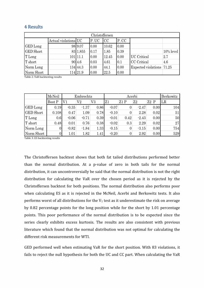
Actual violations UC P. UC CC P. CC

GED Long 98 9.07 0.00 10.62 0.00

GED Short 83 1.855 0.17 1.85 0.39 10% level

T Long 101 11.1 0.00 12.45 0.00 UC Critical 2.7

T short 90 4.6 0.03 4.61 0.1 CC Critical 4.6

Norm Long 134 44.3 0.00 44.1 0.00 Expected violations 71.25

Norm Short 114 21.9 0.00 22.5 0.00

Christoffersen

Table 2: VaR backtesting results

McNeil Berkowitz

Boot P V1 V2 V3 Z1 Z1 P Z2 Z2 P LR

GED Long 0.19 -0.35 -1.37 0.86 -0.07 0 -2.47 0.00 104

GED Short 0.108 0.47 1.09 0.78 -0.10 0 2.28 0.02 51

T Long 0.6 -0.06 -0.71 0.39 -0.01 0.42 -2.43 0.00 50

T short 0.48 0.01 0.76 0.38 -0.02 0.3 2.29 0.02 27

Norm Long 0 -0.82 -1.84 1.33 -0.15 0 -3.15 0.00 754

Norm Short 0 1.01 1.82 1.41 -0.20 0 2.92 0.00 529

Embrechts Acerbi

Table 3: ES backtesting results

The Christoffersen backtest shows that both fat tailed distributions performed better

than the normal distribution. At a p-value of zero in both tails for the normal

distribution, it can uncontroversially be said that the normal distribution is not the right

distribution for calculating the VaR over the chosen period as it is rejected by the

Christoffersen backtest for both positions. The normal distribution also performs poor

when calculating ES as it is rejected in the McNeil, Acerbi and Berkowitz tests. It also

performs worst of all distributions for the V1 test as it underestimate the risk on average

by 0.82 percentage points for the long position while for the short by 1.01 percentage

points. This poor performance of the normal distribution is to be expected since the

series clearly exhibits excess kurtosis. The results are also consistent with previous

literature which found that the normal distribution was not optimal for calculating the

different risk measurements for WTI.

GED performed well when estimating VaR for the short position. With 83 violations, it

fails to reject the null hypothesis for both the UC and CC part. When calculating the VaR

33

on GED long however, it rejects the null hypothesis and thereby further indicating that

the distribution is slightly skewed to the left. This was also indicated in the descriptive

statistics which showed a slight negative skewedness. For the McNeil backtest, the long

position performed better than the short position, which was also the case for the V1,

and Z1 tests. This could be due to the fact that these tests are subordinate VaR and that

the long position has more VaR violations, thereby extreme outliers have less effect on

the results of these tests. Furthermore, the fact that on the V2 test, which is not

subordinate VaR in the same sense, the short position performed better would

strengthen this perceptive. GED, though it outperformed the normal distribution, does

not produce satisfactory results when backtested since all null hypotheses are rejected,

except for VaR on the short position.

Similarly to the GED, the t-distribution produced better VaR estimates on short position

compared to long. However, since the value obtained from the LRuc is 4.6, the null

hypothesis is rejected at a 10% confidence level. For the McNeil test the null hypothesis

is not rejected, indicating that the mean of excess violations is close to zero in both tails.

This is furthermore indicated by the V1 test which estimated that the t-distribution only

underestimate the expected loss by less than 0.07 percentage points in both tails. The

value of the Z1 tests also indicates that the values in both tails that are close to zero. The

Z2 test further strengthens the argument that the mean is close to zero, but that there

are incorrect number of violation in the sample as the Z2 test reject the null hypothesis

while the Z1 does not. Both tails fail the Berkowitz test which is an indication that the

variance in the modified series using the Rosenblatt transformation is not one. This

would indicate that there are outliers that have an extreme effect on the volatility of the

returns. This is not surprising since the oil market is sometimes affected by sudden

jumps due to political events as explained in the introduction. The fat tailed

distributions performed better than the normal distribution. However none of the

distributions performed perfectly on both VaR and ES. Therefore, it would be advisable

for a company to use both GED and t-distribution. It is however, extremely important to

keep in mind the limitations the models have and their inability to foresee the sudden

shocks in the price level.

34

5 Further research This study can be extended in a number of ways. Firstly by using asymmetric

distributions and asymmetric GARCH models. This is a natural extension since the

results and descriptive statistics both showed some signs of negative skewedness.

Another natural extension would be the use of different holding periods as well as

different confidence levels on the risk measurements. This would provide more robust

results as it would offer additional understanding of the behavior of the returns.

6 Conclusion When performing conditional GARCH estimations of VaR and ES on arithmetic returns

for West Texas Intermediate, the fat tailed distributions performed better than the

normal distribution. The t-distribution performed better than GED when calculating ES

which was not expected according to E (i). However when performing the VaR

estimates, the t-distribution did not produce good estimates as both tails fail the

unconditional coverage part of the Christoffersen test. The GED on the other hand

produced better VaR estimates, especially in the right tail. Therefore, the best estimator

for VaR is not the best for ES which is the opposite of was expected by E (ii). It would be

advisable for a company interested estimating the risk of WTI to use both GED and t-

distribution.

35

7 References

Acerbi, Carlo, and Balazs Szekely. "Back-testing expected shortfall." Risk 27.11 (2014).

Almli, Eldar Nikolai, and Torstein Rege. "Risk Modelling in Energy Markets: A Value at

Risk and Expected Shortfall Approach." (2011).

Aloui, Chaker, and Samir Mabrouk. "Value-at-risk estimations of energy commodities via

long-memory, asymmetry and fat-tailed GARCH models." Energy Policy 38.5 (2010):

2326-2339.

Berkowitz, Jeremy. "Testing density forecasts, with applications to risk management."

Journal of Business & Economic Statistics 19.4 (2001): 465-474.

Cheng, Wan-Hsiu, and Jui-Cheng Hung. "Skewness and leptokurtosis in GARCH-typed

VaR estimation of petroleum and metal asset returns." Journal of Empirical Finance 18.1

(2011): 160-173.

Chen, James Ming. "Measuring Market Risk Under the Basel Accords: VaR, Stressed VaR,

and Expected Shortfall." Stressed VaR, and Expected Shortfall (March 19, 2014) 8

(2014): 184-201.

Christoffersen, Peter. "Backtesting." Encyclopedia of Quantitative Finance (2009).

Cont, Rama. "Empirical properties of asset returns: stylized facts and statistical issues."

(2001): 223-236.

Dowd, Kevin. Measuring market risk. John Wiley & Sons, 2005.

Edwards, Davis W. "Energy Trading and Investing." (2010)

Efron, Bradley, and Robert J. Tibshirani. An introduction to the bootstrap. CRC press,

1994.

36

Embrechts, Paul, Roger Kaufmann, and Pierre Patie. "Strategic long-term financial risks:

Single risk factors." Computational Optimization and Applications 32.1-2 (2005): 61-90.

Fattouh, Bassam. An anatomy of the crude oil pricing system. Oxford, England: Oxford

Institute for Energy Studies, 2011

Fan, Ying, et al. "Estimating ‘Value at Risk’of crude oil price and its spillover effect using

the GED-GARCH approach." Energy Economics 30.6 (2008): 3156-3171.

Farzanegan, Mohammad Reza, and Gunther Markwardt. "The effects of oil price shocks

on the Iranian economy." Energy Economics 31.1 (2009): 134-151.

Giot Pierre, and Sébastien Laurent. "Market risk in commodity markets: a VaR

approach." Energy Economics 25.5 (2003):

Hamilton, James Douglas. Time series analysis. Vol. 2. Princeton: Princeton university

press, 1994.

Hung, Jui-Cheng, Ming-Chih Lee, and Hung-Chun Liu. "Estimation of value-at-risk for

energy commodities via fat-tailed GARCH models." Energy Economics 30.3 (2008):

1173-1191.

International Energy Agency (2014) Key World Energy STATISTICS [Online].

Available:

http://www.iea.org/publications/freepublications/publication/KeyWorld2014.pdf

[Accessed 12 May 2015]

Kilian, Lutz. "The economic effects of energy price shocks." (2007).

Lugannani, Robert, and Stephen Rice. "Saddle point approximation for the distribution of

the sum of independent random variables." Advances in applied probability (1980):

475-490.

37

McNeil, Alexander J., and Rüdiger Frey. "Estimation of tail-related risk measures for

heteroscedastic financial time series: an extreme value approach." Journal of empirical

finance 7.3 (2000): 271-300.

Nilsson, Birger( 2014) “Value-at risk” lecture notes in. NEKN83/TEK180 spring 2014.

Lund University

Righi, Marcelo Brutti, and Paulo Sergio Ceretta. "A comparison of Expected Shortfall

estimation models." Journal of Economics and Business 78 (2015): 14-47.

Reider, Rob. "Volatility forecasting I: GARCH models." New York (2009).

Vasudeva, R., and J. Vasantha Kumari. "On general error distributions." 2013

Verbeek, Marno. A guide to modern econometrics. John Wiley & Sons, 2008.

Wong, Woon K. "Backtesting trading risk of commercial banks using expected

shortfall."Journal of Banking & Finance32.7 (2008): 1404-1415.

Xiliang, Zhao, and Zhu Xi. "Estimation of Value-at-Risk for Energy Commodities via

CAViaR Model." Cutting-Edge Research Topics on Multiple Criteria Decision Making.

Springer Berlin Heidelberg, 2009. 429-437.