Copyright

by

Emanuel Gabriel Indrei

2013

The Dissertation Committee for Emanuel Gabriel Indreicertifies that this is the approved version of the following dissertation:

Optimal transport, free boundary regularity, and

stability results for geometric and functional

inequalities

Committee:

Alessio Figalli, Supervisor

Luis A. Caffarelli

Irene M. Gamba

William Beckner

Hans Koch

Jean-Michel Roquejoffre

Optimal transport, free boundary regularity, and

stability results for geometric and functional

inequalities

by

Emanuel Gabriel Indrei, B.S.

DISSERTATION

Presented to the Faculty of the Graduate School of

The University of Texas at Austin

in Partial Fulfillment

of the Requirements

for the Degree of

DOCTOR OF PHILOSOPHY

THE UNIVERSITY OF TEXAS AT AUSTIN

May 2013

to the memory of my brother Marius Christian Indrei

Acknowledgments

It is a pleasure to thank my advisor and friend, Alessio Figalli, for three

years of intellectually stimulating mathematical adventures. He has helped me

grow, both as a mathematician and as an individual. I am in continual awe of

his perspicacity, efficiency, and humility; it is an honor to have been his PhD

student.

Moreover, I feel privileged to have been at Austin concurrently with

Luis Caffarelli. His deep insight in the development of the regularity the-

ory for the Monge-Ampere equation continues to amaze me. Throughout my

graduate studies, I have also benefited from many conversations with Neil

Trudinger on the general optimal transport problem; indeed, to borrow a line

from folklore and slightly modify it: the coldest summer I ever spent was a

winter in Canberra.

During my undergraduate years, I enjoyed many wonderful discussions

with Eric Carlen. I would like to thank Eric for teaching me analysis and for

giving me great advice on various research topics; thanks to him, I have de-

veloped a deep appreciation for mathematical physics, which I hope to further

explore in the future. I would also like to thank Mark Demers for teaching me

about Markov chains and Thomas Morley for serving as my REU mentor.

Moreover, I would like to acknowledge my high school teacher, Matthew

v

Winking, for his enthusiasm in teaching mathematics. He has an extraordinary

ability of making the subject come to life. Indeed, I fondly remember a class

project in which I estimated the height of the building across from our school

by utilizing an angle measuring device and some neat trigonometry.

My undergraduate and graduate experience – which culminated with

this dissertation – was enhanced through my interaction with many individu-

als: Stephanie Weaver, Brian Benson, Sergio Almada, John Widloski, Martin

Mereb, Petar Ivanov, Yuan Yao, Karl Weintraub, Jin Hyuk Choi, Davi Max-

imo, Haotian Wu, Emanuel Carneiro, Veronica Quitalo, Ray Yang, Fernando

Charro, Joao Nogueira, Diego Farias, Levon Nurbekyan, Raf Teymurazyan,

Emily Hannan, Sona Akopian, Sarah Vallelian, Mikel De Viana, Mike Kelly,

Will Carlson, Mihai Sırbu, Anatoly Zlotnik, Karan Odom, Anna Herring . . . ; I

am grateful to these individuals for making the journey so pleasant. Moreover,

I would like to thank Nancy Lamm, Sandra Catlett, and the graduate advisor

Dan Knopf, for their hard work and service to the UT math community.

Finally, I would like to acknowledge my father, Livius, the man whom

I admire more than words can describe, and my sister, Olivia. I thank my

father for being an unceasing source of emotional support and for his continual

encouragement of all my scientific endeavors. His enthusiastic interest in my

research has generated a lot of joy in my life. I thank my sister for her love

and affection and greatly admire her grace and elegance. She has taught

me valuable life lessons which have shaped the individual I am today. I am

incredibly proud to be her brother.

vi

Optimal transport, free boundary regularity, and

stability results for geometric and functional

inequalities

Publication No.

Emanuel Gabriel Indrei, Ph.D.

The University of Texas at Austin, 2013

Supervisor: Alessio Figalli

We investigate stability for certain geometric and functional inequali-

ties and address the regularity of the free boundary for a problem arising in

optimal transport theory. More specifically, stability estimates are obtained

for the relative isoperimetric inequality inside convex cones and the Gaussian

log-Sobolev inequality for a two parameter family of functions. Thereafter,

away from a “small” singular set, local C1,α regularity of the free boundary

is achieved in the optimal partial transport problem. Furthermore, a tech-

nique is developed and implemented for estimating the Hausdorff dimension

of the singular set. We conclude with a corresponding regularity theory on

Riemannian manifolds.

vii

Table of Contents

Acknowledgments v

Abstract vii

Chapter 1. Stability for the relative isoperimetric inequality in-side convex cones 1

1.1 Introduction . . . . . . . . . . . . . . . . . . . . . . . . . . . . 1

1.1.1 Overview . . . . . . . . . . . . . . . . . . . . . . . . . . 1

1.1.2 The anisotropic isoperimetric inequality . . . . . . . . . 5

1.1.3 Sketch of the proof of Theorem 1.1.2 . . . . . . . . . . . 8

1.1.4 Sharpness of the result . . . . . . . . . . . . . . . . . . . 11

1.2 Preliminaries . . . . . . . . . . . . . . . . . . . . . . . . . . . . 13

1.2.1 Initial setup . . . . . . . . . . . . . . . . . . . . . . . . 13

1.2.2 Isoperimetric inequality inside a convex cone . . . . . . 17

1.3 Proof of Theorem 1.1.2 . . . . . . . . . . . . . . . . . . . . . . 22

1.3.1 Main tools . . . . . . . . . . . . . . . . . . . . . . . . . 23

1.3.2 Proof of the result when |α2(E)| is small . . . . . . . . . 43

1.3.3 Reduction step and the conclusion of the proof . . . . . 47

1.4 A sharp quantitative version of the relative Cheeger inequalityinside convex cones . . . . . . . . . . . . . . . . . . . . . . . . 55

Chapter 2. Stability for the log-Sobolev inequality for a twoparameter family of functions 59

2.1 Introduction . . . . . . . . . . . . . . . . . . . . . . . . . . . . 59

2.1.1 Overview . . . . . . . . . . . . . . . . . . . . . . . . . . 59

2.1.2 Main result . . . . . . . . . . . . . . . . . . . . . . . . . 60

2.2 Preliminaries . . . . . . . . . . . . . . . . . . . . . . . . . . . . 61

2.3 Proof of Theorem 2.1.1 . . . . . . . . . . . . . . . . . . . . . . 63

2.4 Controlling the Entropy . . . . . . . . . . . . . . . . . . . . . . 66

viii

Chapter 3. Free boundary regularity in the optimal partial trans-port problem: quadratic cost 69

3.1 Introduction . . . . . . . . . . . . . . . . . . . . . . . . . . . . 69

3.1.1 Overview . . . . . . . . . . . . . . . . . . . . . . . . . . 69

3.1.2 Background . . . . . . . . . . . . . . . . . . . . . . . . . 69

3.2 Preliminaries . . . . . . . . . . . . . . . . . . . . . . . . . . . . 74

3.2.1 Notation . . . . . . . . . . . . . . . . . . . . . . . . . . 75

3.2.2 Basic setup . . . . . . . . . . . . . . . . . . . . . . . . . 77

3.2.3 Tools . . . . . . . . . . . . . . . . . . . . . . . . . . . . 81

3.3 The C1,αloc regularity theory . . . . . . . . . . . . . . . . . . . . 85

3.4 Analysis of the singular set . . . . . . . . . . . . . . . . . . . . 106

Chapter 4. Free boundary regularity in the optimal partial trans-port problem: general cost 131

4.1 Introduction . . . . . . . . . . . . . . . . . . . . . . . . . . . . 131

4.1.1 Overview . . . . . . . . . . . . . . . . . . . . . . . . . . 131

4.1.2 Main result . . . . . . . . . . . . . . . . . . . . . . . . . 131

4.2 Preliminaries . . . . . . . . . . . . . . . . . . . . . . . . . . . . 133

4.3 Regularity theory . . . . . . . . . . . . . . . . . . . . . . . . . 137

4.4 Extensions to Riemannian manifolds . . . . . . . . . . . . . . . 148

Bibliography 153

Vita 161

ix

Chapter 1

Stability for the relative isoperimetric

inequality inside convex cones

1.1 Introduction

1.1.1 Overview

The relative isoperimetric problem inside convex cones is a generaliza-

tion of the classical isoperimetric problem: given an open, convex cone C ⊂ Rn

with n ≥ 2, the task is to identify, under a given volume constraint, the surface

with minimal surface measure in the interior of the cone.1 A version of the

relative isoperimetric problem – known as Dido’s problem – was mentioned by

the ancient Roman poet Virgil in his Aeneid [64]:

“The Kingdom you see is Carthage, the Tyrians, the town of Agenor;

But the country around is Libya, no folk to meet in war.

Dido, who left the city of Tyre to escape her brother,

Rules here–a long and labyrinthine tale of wrong

Is hers, but I will touch on its salient points in order....Dido, in great

disquiet, organized her friends for escape.

1By taking the cone to be Rn, the relative isoperimetric problem reduces to the classicalisoperimetric inequality.

1

They met together, all those who harshly hated the tyrant

Or keenly feared him: they seized some ships which chanced to be ready...

They came to this spot, where to-day you can behold the mighty

Battlements and the rising citadel of New Carthage,

And purchased a site, which was named ’Bull’s Hide’ after the bargain

By which they should get as much land as they could enclose with a bull’s

hide.”

According to legend, Dido cut the oxhide into very thin strips, and

enclosed the largest possible area by laying the tied-together strips in a semi-

circle up against the coast. Indeed, under a fixed perimeter constraint, the

semi-circle encloses the maximal area inside a half-space. Thus, by imagining

the coastal boundary to locally take the form of a line, the heart of Carthage

was in fact the solution to the planar relative isoperimetric problem.

In recent years, there has been a lot of interest in quantitative estimates

for isoperimetric type inequalities [36, 30, 32, 24, 35]. The aim of all of these

results is to show that if a set almost attains the equality in one of these

inequalities, then it is in some sense quantitatively close to a minimizer. Our

goal is to investigate stability for the relative isoperimetric inequality inside

convex cones. The content of this chapter is the subject of a forthcoming

paper co-authored with Alessio Figalli [29]. For related stability results see

also [16, 19, 31, 58].

2

We denote the unit ball in Rn centered at the origin by B1 (similar

notation is used for a generic ball) and the De Giorgi perimeter of E relative

to C by

P (E|C) := sup

∫E

divψdx : ψ ∈ C∞0 (C; Rn), |ψ| ≤ 1

. (1.1)

Mathematically, the relative isoperimetric inequality inside convex cones states

that if E ⊂ C is a Borel set with finite Lebesgue measure |E|, then

n|B1 ∩ C|1n |E|

n−1n ≤ P (E|C). (1.2)

If E has a smooth boundary, the perimeter of E is simply the (n− 1)

– Hausdorff measure of the boundary of E inside the cone (i.e. P (E|C) =

Hn−1(∂E ∩ C)). We also note that if one replaces C by Rn, then the above

inequality reduces to the classical isoperimetric inequality for which there are

many different proofs and formulations (see e.g. [53], [59], [17], [35], [9], [6],

[52]). However, (1.2) is ultimately due to Lions and Pacella [42] (see also [55]

for a different proof using secord order variations). Their proof is based on the

Brunn-Minkowski inequality which states that if A,B ⊂ Rn are measurable,

then

|A+B|1n ≥ |A|

1n + |B|

1n . (1.3)

As we will show below, (1.2) can be seen as an immediate corollary of

the anisotropic isoperimetric inequality (1.7). This fact suggests that there

should also be a direct proof of (1.2) using optimal transport theory (see

3

Theorem 1.2.2), as is the case for the anisotropic isoperimetric inequality [21,

30].

The aim of this chapter is to exploit such a proof in order to establish

a quantitative version of (1.2). To make this precise, we need some more

notation. We define the relative isoperimetric deficit of a Borel set E by

µ(E) :=P (E|C)

n|B1 ∩ C| 1n |E|n−1n

− 1. (1.4)

Note that (1.2) implies µ(E) ≥ 0. The equality cases were considered in [42]

for the special case when C \ 0 is smooth (see also [55]). We will work

out the general case in Theorem 1.2.2 with a self-contained proof. However,

the (nontrivial) equality case is not needed in proving the following theorem

(which is in any case a much stronger statement):

Theorem 1.1.1. Let C ⊂ Rn be an open, convex cone containing no lines,

K = B1 ∩ C, and E ⊂ C a set of finite perimeter with 0 < |E| <∞. Suppose

s > 0 satisfies |E| = |sK|. Then there exists a constant C(n,K) > 0 such that

|E∆(sK)||E|

≤ C(n,K)√µ(E).

The assumption that C contains no lines is crucial. To see this, consider

the extreme case when C = Rn. Let ν ∈ Sn−1 be any unit vector and set

E = 2ν + B1 so that |E∆B1| = 2|B1| > 0. However, µ(E) = 0 so that

in this case Theorem 1.1.1 can only be true up to a translation, and this is

precisely the main result in [30] and [36]. Similar reasoning can be applied

to the case when C is a proper convex cone containing a line (e.g. a half

4

space). Indeed, if C contains a line, then by convexity one can show that (up

to a change of coordinates) it is of the form R × C, with C ⊂ Rn−1 an open,

convex cone. Therefore, by taking E to be a translated version of K along the

first coordinate, the symmetric difference will be positive, whereas the relative

deficit will remain 0.

In general (up to a change of coordinates), every convex cone is of the

form C = Rk×C, where C ⊂ Rn−k is a convex cone containing no lines. Indeed,

Theorem 1.1.1 follows from our main result:

Theorem 1.1.2. Let C = Rk × C, where k ∈ 0, . . . , n and C ⊂ Rn−k is an

open, convex cone containing no lines. Set K = B1 ∩ C, and let E ⊂ C be a

set of finite perimeter with 0 < |E| <∞. Suppose s > 0 satisfies |E| = |sK|.

Then there exists a constant C(n,K) > 0 such that

inf

|E∆(sK + x)|

|E|: x = (x1, . . . , xk, 0, . . . , 0)

≤ C(n,K)

õ(E).

Let us remark that if k = n, then C = Rn and the theorem reduces to

the main result of [30], the only difference being that here we do not attempt

to find any explicit upper bound on the constant C(n,K). However, since

all of our arguments are “constructive,” it is possible to find explicit upper

bounds on C(n,K) in terms on n and the geometry of C (see also §1.1.4).

1.1.2 The anisotropic isoperimetric inequality

As we will show below, our result is strictly related to the quantitative

version of the anisotropic isoperimetric inequality proved in [30]. To show this

5

link, we first introduce some more notation. Suppose K is an open, bounded,

convex set, and let 2

||ν||K∗ := supν · z : z ∈ K. (1.5)

The anisotropic perimeter of a set E of finite perimeter (i.e. P (E|Rn) < ∞)

is defined as

PK(E) :=

∫FE

||νE(x)||K∗dHn−1(x), (1.6)

where FE is the reduced boundary of E, and νE : FE → Sn−1 is the measure

theoretic outer unit normal (see §1.2). Note that for λ > 0, PK(λE) =

λn−1PK(E) and PK(E) = PK(E + x0) for all x0 ∈ Rn. If E has a smooth

boundary, FE = ∂E so that for K = B1 we have PK(E) = Hn−1(∂E).

In general, one can think of || · ||K∗ as a weight function on unit vectors.

Indeed, PK has been used to model surface tensions in the study of equilibrium

configurations of solid crystals with sufficiently small grains (see e.g. [65], [39],

[60]) and also in modeling surface energies in phase transitions (see [38]).

The anisotropic isoperimetric inequality states

n|K|1n |E|

n−1n ≤ PK(E). (1.7)

This estimate (including equality cases) is well known in the literature (see e.g.

[23, 62, 22, 60, 34, 8, 51]). In particular, Gromov [51] uses certain properties

of the Knothe map from E to K in order to establish (1.7). However, as

2Usually in the definition of || · ||K∗ , K is assumed to contain the origin. However, thisis not needed (see Lemma 1.2.1).

6

pointed out in [21] and [30], the argument may be repeated verbatim if one

uses the Brenier map instead. This approach leads to certain estimates which

are helpful in proving a sharp stability theorem for (1.7) (see [30, Theorem

1.1]). The isoperimetric deficit of E is denoted by

δK(E) :=PK(E)

n|K| 1n |E|n−1n

− 1. (1.8)

Note that δK(λE) = δK(E) and δK(E + x0) = δK(E) for all λ > 0

and x0 ∈ Rn. Thanks to (1.7) and the associated equality cases, we have

δK(E) ≥ 0 with equality if and only if E is equal to K (up to a scaling and

translation). Note also the similarity between µ and δK . Indeed, they are both

scaling invariant; however, µ may not be translation invariant (depending on

C). We denote the asymmetry index of E by

A(E) := inf

E∆(x0 + rK)

|E|: x0 ∈ Rn, |rK| = |E|

. (1.9)

The general stability problem consists of proving an estimate of the form

A(E) ≤ CδK(E)1β , (1.10)

where C = C(n,K) and β = β(n,K). In the Euclidean case (i.e. K = B1),

Hall conjectured that (1.10) should hold with β = 2, and this was confirmed

by Fusco, Maggi, Pratelli [36]. Indeed, the 12

exponent is sharp (see e.g. [47,

Figure 4]). Their proof depends heavily on the full symmetry of the Euclidean

ball. For the general case when K is a generic convex set, non-sharp results

were obtained by Esposito, Fusco, Trombetti [24], while the sharp estimate was

7

recently obtained by Figalli, Maggi, Pratelli [30]. Their proof uses a technique

based on optimal transport theory. For more information about the history of

(1.10), we refer the reader to [30] and [47].

1.1.3 Sketch of the proof of Theorem 1.1.2

We now provide a short sketch of the proof of Theorem 1.1.2 for the

case when |E| = |K| and E has a smooth boundary. The first key observation

is that the relative isoperimetric inequality inside a convex cone is a direct

consequence of the anisotropic isoperimetric inequality with K = B1 ∩ C.

Indeed, as follows from the argument in §1.2.2, PK(E) ≤ Hn−1(∂E ∩ C), so

(1.2) follows immediately from (1.7). This observation suggests that one may

exploit Gromov’s argument in a similar way as in the proof of [30, Theorem

1.1] to obtain additional information on E. Indeed, we can show that there

exists a vector α = α(E) ∈ Rn such that 3∫∂E∩C

|1− |x− α||dHn−1 ≤ C(n,K)√δK(E), (1.11)

|E∆(α +K)| ≤ C(n,K)√δK(E). (1.12)

Let us write α = (α1, α2), with α1 ∈ Rk and α2 ∈ Rn−k. Moreover, let E :=

E− (α1, 0). Then using that C = Rk× C, we obtain ∂E∩C− (α1, 0) = ∂E∩C;

therefore, ∫∂E∩C

|1− |x− (0, α2)||dHn−1 ≤ C(n,K)√δK(E), (1.13)

3The existence of a vector α such that (1.12) holds is exactly the main result in [30].However, here we need to show that we can find a vector such that both (1.11) and (1.12)hold simultaneously.

8

|E∆((0, α2) +K)| ≤ C(n,K)√δK(E). (1.14)

Since δK(E) ≤ µ(E) (see Corollary 1.2.3), (1.13) and (1.14) hold with µ(E)

in place of δK(E) (see Lemmas 1.3.5 & 1.3.6). Thanks to (1.14), we see that

our result would readily follow if we can show

|α2| ≤ C(n,K)√µ(E). (1.15)

Indeed, since |((0, α2) +K)∆K| ∼ |α2| (see Lemmas 1.3.1 & 1.3.2),

|E∆K||E|

≤ 1

|K|(|E∆((0, α2) +K)|+ |((0, α2) +K)∆K|

)≤ C(n,K)

õ(E),

which, of course, implies Theorem 1.1.2. Therefore, we are left with proving

(1.15). Firstly, assume that µ(E) and |α2| are sufficiently small (i.e. smaller

than a constant depending only on n and K). By (1.13) and the fact that (see

§1.2)

Hn−1(∂E ∩ (B 34((0, α2)) ∩ C)) = P (E|B 3

4((0, α2)) ∩ C),

we have

C(n,K)√µ(E) ≥

∫∂E∩C

|1− |x− (0, α2)||dHn−1(x)

≥∫∂E∩C∩|1−|x−(0,α2)||≥ 1

4|1− |x− (0, α2)||dHn−1(x)

≥ 1

4Hn−1

(∂E ∩ C ∩

|1− |x− (0, α2)|| ≥ 1

4

)≥ 1

4Hn−1(∂E ∩ (B 3

4((0, α2)) ∩ C))

=1

4P (E|B 3

4((0, α2)) ∩ C).

9

But since |α2| is small, B 12(0) ∩ C ⊂ B 3

4((0, α2)) ∩ C; hence,

P (E|B 34((0, α2)) ∩ C) ≥ P (E|B 1

2(0) ∩ C).

Moreover, thanks to the relative isoperimetric inequality inside B 12(0)∩C (see

e.g. [2, Inequality (3.43)]), we have that for µ(E) small enough,

C(n,K)õ(E)

≥ 1

4c(n,K) min

|E ∩ (B 1

2(0) ∩ C)|

n−1n , |(B 1

2(0) ∩ C) \ E|

n−1n

≥ 1

4c(n,K) min

|E ∩ (B 1

2(0) ∩ C)|, |(B 1

2(0) ∩ C) \ E|

=

1

4c(n,K)|(B 1

2(0) ∩ C) \ E|, (1.16)

where in the last step we used that E is close to (0, α2) + K (see (1.14)) and

|α2| is small. Therefore, using (1.14) and (1.16),

|(B 12(0) ∩ C) \ ((0, α2) +K)| ≤ |(B 1

2(0) ∩ C) \ E|+ |E \ ((0, α2) +K)|

≤ 4C(n,K)

c(n,K)

õ(E) + C(n,K)

õ(E)

≤ C(n,K)√µ(E). (1.17)

Since C contains no lines, by some simple geometric considerations one may

reduce the problem to the case when α2 ∈ (xk+1, . . . , xn) ∈ Rn−k : xn ≥ 0

(see Lemma 1.3.7), and then it is not difficult to prove

c(n,K)|α2| ≤ |(B 12(0) ∩ C) \ ((0, α2) +K)|,

which combined with (1.17) establishes (1.15), and hence, the theorem.

10

Next, we briefly discuss the assumptions for the sketch of the proof

above. Indeed, one may remove the size assumption on |α2| by showing that

if µ(E) is small enough, then |α2| will be automatically small (see Proposition

1.3.11).4 Furthermore, we may freely assume that µ(E) is small since if µ(E) ≥

c(n,K) > 0, then the theorem is trivial:

|E∆(sK)||E|

≤ 2 ≤ 2√c(n,K)

õ(E).

The regularity of E was used in order to apply the Sobolev-Poincare type

estimate [30, Lemma 3.1] which yields (1.13) (see Lemma 1.3.5). If E is a

general set of finite perimeter in C with finite mass and small relative deficit,

then Lemma 1.3.4 tells us that E has a sufficiently regular subset G so that |E\

G| and µ(G) are controlled by µ(E). Combining this fact with the argument

above yields the theorem for general sets of finite perimeter (see Proposition

1.3.8). Lastly, the assumption on the mass of E (i.e. |E| = |K|) can be

removed by a simple scaling argument.

1.1.4 Sharpness of the result

We now discuss the sharpness of the estimate in Theorem 1.1.2. Indeed,

it is well known that there exists a sequence of ellipsoids Ehh∈N, symmetric

4Let us point out that this is a nontrivial fact. Indeed, in our case we want to provein an explicit, quantitative way that µ(E) controls α2(E); hence, we want to avoid anycompactness argument. However, even using compactness, we do not know any simpleargument which shows that α2(E)→ 0 as µ(E)→ 0.

11

with respect to the origin and converging to the ball B1, such that

limh→∞

sup

√δB1(Eh)

|Eh∆(shB1)|<∞, lim

h→∞δK0(Eh) = 0,

where sh =

(|Eh||B1|

) 1n

(see e.g. [48, pg. 382]). Consider the cone C = x ∈

Rn : x1, . . . , xn > 0 and set Eh := Eh ∩ C. By symmetry, it follows that

δB1(Eh) = 12nδB1(Eh) and |Eh∆(shK)| = 1

2n|Eh∆(shB1)|. We also note that

P (Eh|C) = Hn−1(∂Eh ∩ C) =1

2nHn−1(∂Eh) =

1

2nPB1(Eh),

|Eh| =1

2n|Eh|, |B1 ∩ C| = 1

2n|B1|.

Therefore,

µ(Eh) =P (Eh|C)

n|B1 ∩ C| 1n |Eh|n−1n

− 1 =1

2nHn−1(∂Eh)

n( 12n|B1|)

1n ( 1

2n|E|)n−1

n

− 1

=PB1(Eh)

n|B1 ∩ C| 1n |Eh|n−1n

− 1 = δB1(Eh),

and we have

limh→∞

sup

õ(Eh)

|Eh∆(shK)|<∞.

This example shows that the 12

exponent in the theorem cannot, in general,

be replaced by something larger.

One may wonder whether it is possible for Theorem 1.1.2 to hold with

a constant depending only on the dimension and not on the cone. Indeed, in

[30, Theorem 1.1], the constant does not depend on the convex set associated

12

to the anisotropic perimeter. However, this is not so in our case. To see this,

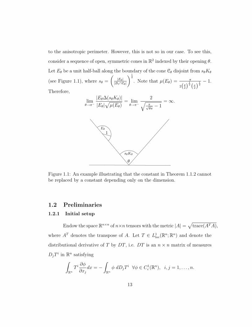
consider a sequence of open, symmetric cones in R2 indexed by their opening θ.

Let Eθ be a unit half-ball along the boundary of the cone Cθ disjoint from sθKθ

(see Figure 1.1), where sθ =

(|Eθ||B1∩Cθ|

) 12

. Note that µ(Eθ) = π

2(θ2

) 12(π2

) 12− 1.

Therefore,

limθ→π−

|Eθ∆(sθKθ)||Eθ|

√µ(Eθ)

= limθ→π−

2√π√θπ− 1

=∞.

Figure 1.1: An example illustrating that the constant in Theorem 1.1.2 cannotbe replaced by a constant depending only on the dimension.

1.2 Preliminaries

1.2.1 Initial setup

Endow the space Rn×n of n×n tensors with the metric |A| =√

trace(ATA),

where AT denotes the transpose of A. Let T ∈ L1loc(Rn; Rn) and denote the

distributional derivative of T by DT , i.e. DT is an n× n matrix of measures

DjTi in Rn satisfying∫

RnT i∂φ

∂xjdx = −

∫Rnφ dDjT

i ∀φ ∈ C1c (Rn), i, j = 1, . . . , n.

13

If C ⊂ Rn is a Borel set, then DT (C) is the n × n tensor whose entries are

given by(DjT

i(C))i,j=1,...,n

, and |DT |(C) is the total variation of DT on C

with respect to the metric defined above, i.e.

|DT |(C) = sup

∑h∈N

∑ij

|DiTj(Ch)| : Ch ∩ Ck = ∅,

⋃h∈N

Ch ⊂ C

.

Let BV (Rn; Rn) be the set of all T ∈ L1(Rn; Rn) with |DT |(Rn) < ∞. For

such a T , decompose DT = ∇Tdx + DsT , where ∇T is the density with

respect to the Lebesgue measure and DsT is the corresponding singular part.

Denote the distributional divergence of T by Div T := trace(DT ), and let

div(T ) := trace(∇T (x)). Then we have Div T = div Tdx+ trace(DsT ). If DT

is symmetric and positive definite, note that

trace(DsT ) ≥ 0. (1.18)

If E is a set of finite perimeter in Rn, then the reduced boundary FE

of E consists of all points x ∈ Rn such that 0 < |D1E|(Br(x)) < ∞ for all

r > 0 and the following limit exists and belongs to Sn−1:

limr→0+

D1E(Br(x))

|D1E|(Br(x))=: −νE(x).

We call νE the measure theoretic outer unit normal to E. By the well-known

representation of the perimeter in terms of the Hausdorff measure, one has

P (E|C) = Hn−1(FE∩C) (see e.g. [2, Theorem 3.61] and [2, Equation (3.62)]).

This fact along with one of the equality cases in (1.2) – n|B1∩C| = Hn−1(∂B1∩

C) – yields the following useful representation of the relative deficit (recall that

14

s > 0 satisfies |E| = |sK|):

µ(E) =Hn−1(FE ∩ C)−Hn−1(∂Bs ∩ C)

Hn−1(∂Bs ∩ C). (1.19)

Next, if T ∈ BV (Rn; Rn), then for Hn−1- a.e. x ∈ FE there exists an

inner trace vector trE(T )(x) ∈ Rn (see [2, Theorem 3.77]) which satisfies

limr→0+

1

rn

∫Br(x)∩y:(y−x)·νE(x)<0

|T (y)− trE(T )(x)|dy = 0.

Furthermore, E(1) denotes the set of points in Rn having density 1 with respect

to E; i.e. x ∈ E(1) means

limr→0+

|E ∩Br(x)||Br(x)|

= 1.

Having developed the necessary notation, we are ready to state the

following general version of the divergence theorem (see e.g. [2, Theorem

3.84]) which will help us prove the isoperimetric inequality for convex cones

(i.e. Theorem 1.2.2):

Div T (E(1)) =

∫FE

trE(T )(x) · νE(x)dHn−1(x). (1.20)

Now we develop a few more tools that will be used throughout the

chapter. Fix K := B1 ∩ C, and let

D := E ⊂ C : P (E|C) <∞, |E| <∞.

To apply the techniques in [30], we need a convex set that contains the origin.

Therefore, let us translate K by the vector x0 ∈ −K which minimizes the ratio

15

MK0

mK0, where K0 = K + x0,

mK0 := inf||ν||K0∗ : ν ∈ Sn−1 > 0, MK0 := sup||ν||K0∗ : ν ∈ Sn−1 > 0,

(1.21)

and ||ν||K0∗ is defined as in (1.5). Next, we introduce the Minkowski gauge

associated to the convex set K0:

||z||K0 := inf

λ > 0 :

z

λ∈ K0

. (1.22)

Note that the convexity of K0 implies the triangle inequality for || · ||K0 so that

it behaves sort of like a norm; however, if K0 is not symmetric with respect

to the origin, ||x||K0 6= || − x||K0 . Hence, this “norm” is in general not a

true norm. Nevertheless, the following estimates relate this quantity with the

standard Euclidean norm | · | (see [30, Equations (3.2) and (3.9)]):

|x|MK0

≤ ||x||K0 ≤|x|mK0

, (1.23)

||y||K0∗ ≤MK0

mK0

|| − y||K0∗. (1.24)

Recall that the isoperimetric deficit δK(·) is scaling and translation

invariant in its argument. The next lemma states that it is also translation

invariant in K (observe that if z0+K does not contain the origin, then ||·||z0+K

can also be negative in some direction).

Lemma 1.2.1. Let E ∈ D. Then δz0+K(E) = δK(E) for all z0 ∈ Rn.

16

Proof. It suffices to prove Pz0+K(E) = PK(E).

Pz0+K(E) =

∫FE

supνE(x) · z : z ∈ z0 +KdHn−1(x)

=

∫FE

supνE(x) · (z0 + z) : z ∈ KdHn−1(x)

=

∫FE

(νE(x) · z0 + supνE(x) · z : z ∈ K)dHn−1(x)

=

∫FE

νE(x) · z0dHn−1(x) + PK(E).

By using the divergence theorem for sets of finite perimeter [2, Equation

(3.47)], we obtain∫FE

νE(x) · z0dHn−1(x) =

∫E

div(z0)dx = 0,

which proves the result.

1.2.2 Isoperimetric inequality inside a convex cone

Here we show how to use Gromov’s argument to prove the relative

isoperimetric inequality for convex cones. As discussed in the introduction,

the first general proof of the inequality is due to Lions and Pacella [42] and

employs the Brunn-Minkowski inequality. The equality cases were considered

in [42] for the special case when C\0 is smooth. Our proof of the inequality

closely follows the proof of [30, Theorem 2.3] with some minor modifications.

Theorem 1.2.2. Let C be an open, convex cone and |E| <∞. Then

n|E|n−1n |K|

1n ≤ Hn−1(FE ∩ C). (1.25)

17

Moreover, if C contains no lines, then equality holds if and only if E = sK.

Proof.

Proof of (1.25). By rescaling, if necessary, we may assume that |K| =

|E| (i.e. s = 1). Define the probability densities dµ+(x) = 1|E|1E(x)dx and

dµ−(y) = 1|K|1K(y)dy. By classical results in optimal transport theory, it is

well known that there exists an a.e. unique map T : E → K (which we call

the Brenier map) such that T = ∇φ where φ is convex, T ∈ BV (Rn;K), and

det(∇T (x)) = 1 for a.e. x ∈ E (see e.g. [7, 49, 50, 1]). Moreover, since T is

the gradient of a convex function with positive Jacobian, ∇T (x) is symmetric

and nonnegative definite; hence, its eigenvalues λk(x) are nonnegative for a.e.

x ∈ Rn. As a result, we may apply the arithmetic-geometric mean inequality

to conclude that for a.e. x ∈ E,

n = n(det∇T (x)

) 1n = n

( n∏k=1

λk(x)

) 1n

≤n∑k=1

λk(x) = div T (x). (1.26)

Therefore,

n|E|n−1n |K|

1n = n|E| = n

∫E

det(∇T (x))1ndx

≤∫E

div T (x)dx =

∫E(1)

div T (x)dx, (1.27)

where we recall that E(1) denotes the set of points with density 1 (see §1.2).

Next, we use (1.18) and (1.20):∫E(1)

div T (x)dx ≤∫E(1)

div T (x)dx+ (Div T )s(E(1))

= Div T (E(1)) =

∫FE

trE(T )(x) · νE(x)dHn−1(x). (1.28)

18

By the convexity of K and the fact that T (x) ∈ K for a.e. x ∈ E, it follows

that trE(T )(x) ∈ K, so by the definition of || · ||K∗ ,

trE(T )(x) · νE(x) ≤ ||νE(x)||K∗.

Hence,∫FE

trE(T )(x) · νE(x)dHn−1(x) ≤∫

FE

||νE(x)||K∗dHn−1(x) = PK(E). (1.29)

Furthermore, note that if z ∈ K, then |z| ≤ 1; therefore,

||νE(x)||K∗ = supνE(x) · z : z ∈ K ≤ 1.

Moreover, observe that by the definition of || · ||K∗, it follows easily that

||νC(x)||K∗ = 0 for Hn−1 -a.e. x ∈ ∂C \ 0; therefore, ||νE(x)||K∗ = 0 for

Hn−1 -a.e. x ∈ FE ∩ ∂C. Thus,∫FE

||νE(x)||K∗dHn−1(x) =

∫FE∩C

||νE(x)||K∗dHn−1(x) ≤ Hn−1(FE ∩ C),

and this proves the inequality.

Equality case. If E = K, then T (x) = x and it is easy to check that equality

holds in each of the inequalities above. Conversely, suppose there is equality.

In particular, n|K| = PK(E). By [34] (see also [30, Theorem A.1]), we obtain

that E = K + a with a ∈ C. Suppose a 6= 0. Then since C + a ⊂ C, we have

∂K ∩ C ⊂ ∂K ∩ (C− a). But

Hn−1(∂K ∩ C) = n|K| = Hn−1(∂(K + a) ∩ C) = Hn−1(∂K ∩ (C− a)).

19

Therefore,

∂K ∩ C = ∂K ∩ (C− a). (1.30)

Now, note that for t ≥ 1, we also have C− a ⊂ C− ta. In fact, we claim

∂K ∩ (C− a) = ∂K ∩ (C− ta). (1.31)

Indeed, if not, then there exists x ∈ ∂K such that x ∈ (C − ta) \ (C − a).

In particular, t > 1 and thanks to (1.30) we have that x /∈ C; therefore,

x ∈ ∂K ∩ ∂C ∩ (C− ta) and we may write x = c− ta for some c ∈ C, so that

x =1

t(c− ta) +

(1− 1

t

)x =

(c

t+

(1− 1

t

)x

)− a.

But since x ∈ ∂C, c ∈ C, and t > 1, it follows that(ct

+ (1 − 1t)x)∈ C; thus,

x ∈ C− a, a contradiction. Therefore, if we let C∞ :=⋃t≥1

(C− ta), then thanks

to (1.30) and (1.31) we obtain

∂K ∩ C = ∂K ∩ C∞ =((∂B1 ∩ C) ∩ C∞

)∪((B1 ∩ ∂C) ∩ C∞

).

This implies

B1 ∩ ∂C ∩ C∞ = ∅. (1.32)

Next, we note that C∞ is a convex cone: indeed, if x ∈ C∞ and λ > 0, then

λx = λc − λta = (λc + a) − (1 + λt)a ∈ C∞. Likewise, if x, y ∈ C∞ and

λ ∈ [0, 1], then λx + (1− λy) = λ(c1 − t1a) + (1− λ)(c2 − t2a) = (λc1 + (1−

λ)c2 + λt2a)− (λt1 + t2)a ∈ C∞. Thus, since C∞ is a convex cone, (1.32) gives

∂C ∩ C∞ = ∅. (1.33)

20

Note that C ⊂ C∞. If x ∈ C∞\C, then pick a point y ∈ C. Since λx+(1−λ)y ∈

C∞ for all λ ∈ [0, 1], we obtain that ∂C ∩ C∞ 6= ∅, contradicting (1.33).

Therefore, C = C∞, but this is a contradiction since C∞ contains the line

tat∈R. Hence, a = 0 and we are done.

Corollary 1.2.3. If E ∈ D, then δK(E) ≤ µ(E).

Proof. Since the inequality is scaling invariant, we may assume that |E| = |K|.

From (1.29) and the fact that n|K| = Hn−1(∂B1 ∩ C) we obtain

PK(E)− n|K| ≤ Hn−1(FE ∩ C)− n|K| = Hn−1(FE ∩ C)−Hn−1(∂B1 ∩ C).

Dividing by n|K| and using the representation of µ(E) given by (1.19) yields

the result.

Corollary 1.2.4. Let E ∈ D with |E| = |K|, and let T0 : E → K0 be the

Brenier map from E to K0. Then∫FE∩C

(1− | trE(T0 − x0)(x)|

)dHn−1(x) ≤ n|K|µ(E).

Proof. Let T : E → K be the Brenier map from E to K so that T is the a.e.

unique gradient of a convex function φ. Then T0(x) = T (x) + x0 (this follows

easily from the fact that T (x) + x0 = ∇φ(x) + x0 = ∇(φ(x) + x0 · x) and

φ(x) + x0 · x is still convex). Therefore, by (1.27) and (1.28),

n|E| ≤∫

FE

trE(T0 − x0)(x) · νE(x)dHn−1(x). (1.34)

21

Next, we recall from the proof of Theorem 1.2.2 that trE(T0 − x0)(x) ∈ K.

Hence, trE(T0 − x0)(x) · νE(x) ≤ 0 for Hn−1 a.e. x ∈ FE ∩ ∂C and | trE(T0 −

x0)(x)| ≤ 1 for Hn−1 a.e. x ∈ FE ∩ C. Therefore, using (1.34),

n|E| ≤∫

FE∩C

trE(T0 − x0)(x) · νE(x)dHn−1(x)

≤∫

FE∩C

| trE(T0 − x0)(x)|dHn−1(x) ≤ Hn−1(FE ∩ C).

The fact that n|E| = n|K| = Hn−1(∂B1 ∩ C) finishes the proof.

1.3 Proof of Theorem 1.1.2

We split the proof in several steps. In §1.3.1, we collect some useful

technical tools. Then in §1.3.2, we prove Theorem 1.1.2 under the additional

assumption that E is close to K (up to a translation in the first k coordinates).

Finally, we remove this assumption in §1.3.3 to conclude the proof of the

theorem.

Let eknk=1 be the standard orthonormal basis for Rn. Recall that

C = Rk × C, where C ⊂ Rn−k is an open, convex cone containing no lines.

Hence, up to a change of coordinates, we may assume without loss generality

that ∂C ∩ xn = 0 = 0. With this in mind and a simple compactness

argument, we note that

b = b(n,K) := inft > 0 : ∂B 12(0) ∩ C ∩ xn < t 6= ∅ > 0, (1.35)

where B 12(0) is the ball in Rn−k. Indeed, if not, then for a minimizing sequence

tk, we may find corresponding zk ∈ ∂B 12∩C∩xn < tk. Along a subsequence

22

(still indexed by k), we have zk → z, with |z| = 12. Denote the nth component

of zk by zkn, so that 0 < zkn < tk → 0. Therefore, z 6= 0, z ∈ ∂C and zn = 0, a

contradiction. Thus, (1.35) is established.

Next, we introduce the trace constant of a set of finite perimeter. Recall

the definition of K0 given in §2.1, so that (1.23) and (1.24) hold. Given a set

E ∈ D, let τ(E) denote the trace constant of E, where

τ(E) := inf

PK0(F )∫

FF∩FE||νE||K0∗dH

n−1: F ⊂ E, |F | ≤ |E|

2

. (1.36)

Note that τ is scaling invariant, and in general τ(E) ≥ 1. The trace constant

contains valuable information about the geometry of E. For example, if E has

multiple connected components or outward cusps, then τ(E) = 1. In general,

sets for which τ(E) > 1 enjoy a nontrivial Sobolev-Poincare type inequality

(see [30, Lemma 3.1]).

1.3.1 Main tools

In what follows, we develop some technical tools needed in order to

prove Theorem 1.1.2. The following two lemmas are general facts about sets

of finite perimeter, see [29, Lemmas 3.1 & 3.2]. However, for our purpose, we

only need them to be true for open, bounded, convex sets; thus, we prefer to

give alternate geometric proofs.

Lemma 1.3.1. Let A ⊂ Rn be an open, bounded, convex set. Then there

exists C1.3.1(n,A) > 0 such that for any y ∈ Rn, |(y+A)∆A| ≤ C1.3.1(n,A)|y|.

23

Proof. If |y| > diam(A), then |(y + A)∆A| = 2|A|, and |(y + A)∆A| ≤2|A|

diam(A)|y|. Next, suppose |y| ≤ diam(A). Note that for any z0 ∈ Rn,

|(y + A)∆A| = |(y + (A+ z0))∆(A+ z0)|,

therefore we may assume without loss of generality that A contains the origin.

Then the assumptions on A imply the triangle inequality for || · ||A. Hence, if

x ∈ A, by (1.23) we have ||y + x||A < ||y||A + 1 ≤ 1mA|y| + 1. Therefore, it is

sufficient to dilate A by 1mA|y| + 1 in order for y + A ⊂ (1 + 1

mA|y|)A. Since

|y + A| = |A| and |y| ≤ diam(A), we have that

|(y + A)∆A| = 2|(y + A) \ A| ≤ 2∣∣(1 +

1

mA

|y|)A \ A∣∣

= 2(∣∣(1 +

1

mA

|y|)A∣∣− |A|) = 2((1 +

1

mA

|y|)n − 1)|A|

≤ C(n,A)|y|.

Note that it is easy to find an explicit upper bound on C(n,A) by using the bi-

nomial expansion (since |y| ≤ diam(A)). Therefore, we may take C1.3.1(n,A) =

max 2|A|diam(A)

, C(n,A).

Lemma 1.3.2. Let A ⊂ Rn be an open, bounded, convex set. Then there exist

two constants C1.3.2(n,A), c1.3.2(n,A) > 0 such that if y ∈ Rn, then

minc1.3.2(n,A), C1.3.2(n,A)|y| ≤ |(y + A)∆A|.

Proof. For t > 0 and w ∈ Sn−1 let

fw(t) := |(A+ tw)∆A|.

24

Note that fw(t) =∫

Rn |1(A+tw)(x) − 1A(x)|dx =∫

Rn |1A(x + tw) − 1A(x)|dx.

Furthermore, for t > 0, let

gw(t) :=

∫∂(A−tw)∩A

〈νA(x+ tw), w〉dHn−1(x),

where νA is the outer unit normal to the boundary of A. Our strategy is

as follows: first we show that gw(t) has a positive lower bound for all t > 0

sufficiently small that is also uniform in w ∈ Sn−1. Then we prove f ′w(t) =

2gw(t) for almost every t. Since fw is Lipschitz, this will conclude the proof.

The idea of the proof for the first part is simple though the precise argument

is a bit technical: for fixed w and t, by convexity, it follows that there is

a set M(w,t) ⊂ ∂A so that M(w,t) − tw ⊂ ∂(A − tw) ∩ A and on which the

angle between normal vectors and w is uniformly bounded away from π2

(see

Figure 1.2). However, by compactness of ∂A, one can show that Hn−1(M(w,t))

is uniformly bounded from below by a positive constant independent of w and

t and this yields a uniform lower bound on gw(t).

To begin, we claim that for s > 0, if 0 < t < s, then

∂(A− sw) ∩ A+ (s− t)w ⊂ ∂(A− tw) ∩ A. (1.37)

Indeed, let x = y + (s − t)w with y ∈ ∂(A − sw) ∩ A. Thus, y = a − sw,

with a ∈ ∂A and so x = a − tw. Since y ∈ A, convexity tells us that for all

λ ∈ (0, 1),

λy + (1− λ)a ∈ A.

But λy + (1 − λ)a = λ(a − sw) + (1 − λ)a = a − λsw. By letting λ = ts

we

see a − tw = x ∈ A, and this completes the proof of the claim. Note that by

25

Figure 1.2: Controlling gw(t) from below.

the convexity of A, we also have 〈νA(x+ tw), w〉 ≥ 0 for all x ∈ (∂A− tw)∩A

(indeed, if y ∈ ∂A and νA(y) · w < 0, then y − tw ∈ z : 〈z − y, νA(y)〉 > 0,

and the latter is disjoint from A). Therefore, by the change of variable x =

y + (s− t)w and (1.37), it follows that

gw(s) =

∫∂(A−sw)∩A

〈νA(y + sw), w〉dHn−1(y)

=

∫∂(A−sw)∩A+(s−t)w

〈νA(x+ tw), w〉dHn−1(x)

≤ gw(t),

provided 0 < t < s. Next, we claim that for a particular value of s = s(n,A) >

0 (which we will specify later),

infw∈Sn−1

gw(s) > 0. (1.38)

Indeed, let w ∈ Sn−1, and for each point y ∈ ∂A find ry > 0 so that Bry(y)∩∂A

is the graph of a concave function uy : Rn−1 → R. Upon a possible relabeling

26

and reorientation of the coordinate axes, we have

A ∩Bry(y) = x ∈ Bry(y) : xn < uy(x1, . . . , xn−1).

In what follows, Bβ(α) denotes the open ball in Rn−1 centered at α with radius

β. Since

∂A ⊂⋃y∈∂A

Bry/2(y),

by compactness of ∂A there exists N ∈ N and ykNk=1 ⊂ ∂A such that ∂A ⊂

∪Nk=1Brk/2(yk). Denote the corresponding concave functions by ukNk=1, with

the understanding that ∂A ∩Brk(yk) is the graph of uk. Next, let y∗ ∈ ∂A be

such that the normal to one of the supporting hyperplanes at y∗ is w. Then

y∗ ∈ ∂A ∩ Brj/2(yj) for some j ∈ 1, 2, . . . , N. Moreover, uj : Brj(xj) → R,

where (xj, uj(x)) = yj, and

A ∩Brj(yj) = x ∈ Brj(y) : xn < u(x1, . . . , xn−1). (1.39)

Next, let x∗ ∈ Brj/2(xj) be such that (x∗, uj(x∗)) = y∗, r = r(n,A) :=

minkrk/4, and s = s(n,A) := r/4. Since x∗ ∈ Brj/2(xj), we have Br(x

∗) ⊂

B3rj/4(xj). Let us denote the superdifferential of a concave function φ : Rn−1 →

R at a point x in its domain by

∂+φ(x) := y ∈ Rn−1 : ∀z ∈ Rn−1, φ(z) ≤ φ(x) + 〈y, z − x〉.

Since w is the normal to a supporting hyperplane of A at (x∗, uj(x∗)), there

exists∇+uj(x∗) ∈ ∂+uj(x

∗) such that w =(−∇+uj(x

∗),1)√1+|∇+uj(x∗)|2

=: (w, w⊥). Up to an

infinitesimal rotation, we can assume without loss of generality |∇+uj(x∗)| > 0.

27

Let e1 =∇+uj(x

∗)|∇+uj(x∗)| and e2, . . . , en−1 be a corresponding orthonormal basis

for Rn−1. We define

Nε :=

z ∈ Br(x

∗) : z − x∗ = γ1e1 +n−1∑i=2

γiei,∣∣ n−1∑i=2

γiei∣∣ ≤ ε, −r

4≥ γ1

,

and

Nε :=

z ∈ Br(x

∗) : z − x∗ = γ1e1 +n−1∑i=2

γiei,∣∣ n−1∑i=2

γiei∣∣ ≤ ε, −r

2≥ γ1

.

Let z ∈ Nε, and note that

uj(z) ≤ uj(z − sw) + 〈∇+uj(z − sw), sw〉

= uj(z − sw)− s√1 + |∇+uj(x∗)|2

〈∇+uj(z − sw),∇+uj(x∗)〉. (1.40)

Furthermore, if z ∈ Br(x∗), then there exists ∇+uj(z) ∈ ∂+uj(z) such that

νA((z, uj(z))) =(−∇+uj(z),1)√

1+|∇+uj(z)|2. Thus,

〈νA((z, uj(z))), w〉 =

⟨(−∇+uj(z), 1)√1 + |∇+uj(z)|2

,(−∇+uj(x

∗), 1)√1 + |∇+uj(x∗)|2

⟩=

1 +∇+uj(z) · ∇+uj(x∗)√

1 + |∇+uj(z)|2√

1 + |∇+uj(x∗)|2(1.41)

If C = maxkLip 3

4(uk) > 0, where Lip 3

4(uk) denotes the Lipschitz constant of

uk on B 34rk

(xk) (recall xk := u−1k (yk)), then since sup

z∈Br(x∗)|∇+uj(z)| ≤ C, we

have

1√1 + |∇+uj(z)|2

√1 + |∇+uj(x∗)|2

≥ 1

1 + C2=: C0. (1.42)

Next, the monotonicity formula for the superdifferential of the concave func-

tion uj tells us that

〈∇+uj(z)−∇+uj(x∗), z − x∗〉 ≤ 0,

28

and since 〈∇+uj(x∗), z − x∗〉 ≤ 0 for z ∈ Nε, we have

0 ≥ 〈∇+uj(z), z − x∗〉 = 〈∇+uj(z), γ1e1 +n−1∑i=2

γiei〉

≥ γ1

|∇+uj(x∗)|〈∇+uj(z),∇+uj(x

∗)〉 − C0ε.

As 0 < r4≤ −γ1 we obtain

〈∇+uj(z),∇+uj(x∗)〉 ≥ −4C0ε|∇+uj(x

∗)|r

≥ −4C0Cε

r. (1.43)

Note that if z ∈ Nε, then z − sw ∈ Nε so by (1.43)

〈∇+uj(z − sw),∇+uj(x∗)〉 ≥ −4C0Cε

r.

Combining this with (1.40) yields

uj(z − sw) ≥ uj(z)− s 4C0Cε

r√

1 + |∇+uj(x∗)|2≥ uj(z)− s4C0Cε

r. (1.44)

Now pick ε ∈(0,min r

4C0C√

1+C2 ,r

8C0C). Note that ε = ε(n,A) and with this

choice of ε, (1.41), (1.42), and (1.43) imply that for z ∈ Nε,

〈νA((z, uj(z))), w〉 ≥ 1

2C0, (1.45)

whereas (1.44) implies

uj(z − sw) > uj(z)− s√1 + C2

≥ uj(z)− sw⊥. (1.46)

From (1.46), we obtain (z − sw, uj(z)− sw⊥) ∈ ∂(A− sw)∩A. Moreover, let

Us : Rn−1 → Rn be given by Us(d) = (d, uj(d+ sw)− sw⊥). Then

Us(Nε − sw) ⊂ ∂(A− sw) ∩ A. (1.47)

29

Therefore, if y ∈ Us(Nε − sw) so that y = (z − sw, uj(z) − sw⊥) for some

z ∈ Nε, then ν(A−sw)(y) = νA((z, uj(z))); hence, (1.45) implies

〈ν(A−sw)(y), w〉 = 〈νA((z, uj(z)), w〉 ≥ 1

2C0.

This fact and (1.47) yields

gs(w) =

∫∂(A−sw)∩A

〈νA−sw(y), w〉dHn−1(y)

≥∫Us(Nε−sw)

1

2C0dH

n−1(y) =1

2C0H

n−1(Us(Nε − sw))

≥ 1

2C0H

n−1(Nε − sw) ≥ 1

2C0γ(n, ε)rn−1 =

1

2C0γ(n, ε) min

k

(rk4

)n−1

,

and this proves (1.38). Next, we claim f ′w(t) = 2gw(t) almost everywhere. To

see this, let

h(y) := |A \ (A− y)| =∫

Rn1A\(A−y)(x)dx,

and ψ ∈ C∞c (Rn; Rn). By Lemma 1.3.1, h(y) is Lipschitz; therefore, using

integration by parts, Fubini, and that ψ is divergence free we obtain∫Rnψ · ∇h(y)dy = −

∫Rn

divψ(y)h(y)dy

= −∫

Rn

(∫Rn

divψ(y)1A\(A−y)(x)dy

)dx

= −∫A

(∫Rn

divψ(y)1A\(A−y)(x)dy

)dx

= −∫A

(∫Rn

divψ(y)(1− 1(A−y)(x))dy

)dx

=

∫A

(∫Rn

divψ(y)1(A−y)(x)dy

)dx. (1.48)

30

Next, note that 1(A−y)(x) = 1(A−x)(y) and by applying the divergence theorem,

it follows that∫Rn

divψ(y)1(A−x)(y)dy =

∫Rn〈ψ(y), ν(A−x)(y)〉dHn−1b∂(A− x)(y)

=

∫Rn〈ψ(z − x), νA(z)〉dHn−1b∂A(z). (1.49)

Hence, by (1.48), (1.49), and Fubini we obtain∫Rnψ · ∇h(y)dy =

∫A

(∫Rn〈ψ(z − x), νA(z)〉dHn−1b∂A(z)

)dx

=

∫Rn

(∫Rnψ(z − x)1A(x)dx

)· νA(z)dHn−1b∂A(z)

=

∫Rn

(∫Rnψ(y)1A(z − y)dy

)· νA(z)dHn−1b∂A(z)

=

∫Rnψ(y) ·

(∫Rn

1A(z − y)νA(z)dHn−1b∂A(z)

)dy

=

∫Rnψ(y) ·

(∫∂(A−y)

1A(x)νA(x+ y)dHn−1(x)

)dy.

But, since ψ ∈ C∞c (Rn; Rn) is arbitrary, we have that for a.e. y ∈ Rn,

∇h(y) =

∫∂(A−y)∩A

ν(A−y)(x)dHn−1(x).

Note that fw(t) = 2h(tw), and since fw(t) is Lipschitz, for a.e. t ∈ R we have

f ′w(t) = 2∇h(tw) · w = 2gw(t).

Now we can finish the proof: let y ∈ Rn, and write y = tw for some w ∈ Sn.

If t ∈ [0, s], then

fw(t) =

∫ t

0

f ′w(ξ)dξ =

∫ t

0

2gw(ξ)dξ ≥ 2 infw∈Rn

gw(s)t

= 2 infw∈Rn

gw(s)|y|.

31

Let C1.3.2(n,A) := 2 infw∈Rn

gw(s), and note that C1.3.2(n,A) > 0 thanks to (1.38).

Thus, for |y| ≤ s = s(n,A),

C1.3.2(n,A)|y| ≤ |(A+ y)∆A|.

If |y| > s, then using that fw is a non-decreasing function and the previous

inequality, we obtain

C1.3.2(n,A)s = C1.3.2(n,A)

∣∣∣∣s y|y|∣∣∣∣ ≤ ∣∣∣∣(A+ s

y

|y|)∆A

∣∣∣∣ ≤ |(A+ y)∆A|.

Therefore, C1.3.2(n,A) mins, |y| ≤ |(A+ y)∆A|.

Lemma 1.3.3. There exists a bounded, convex set K ⊂ B 12(0)∩ C so that for

all y = (0, . . . , 0, yk+1, . . . , yn) with yn ≥ 0, we have

K \ (y + K) = K \ (y + C). (1.50)

Furthermore, if yn ≤ 0, then

(y + K) \ K = (y + K) \ C. (1.51)

Proof. We will show that one may pick b = b(n,K) > 0 small enough so that

K := B 12(0) ∩ C ∩

(∩ki=1 |xi| < b

)∩ xn < b

has the desired properties. We will establish (1.50) first. Since y+ K ⊂ y+ C,

it suffices to prove K \ (y + K) ⊂ K \ (y + C). If (by contradiction) there

exists x ∈ K ∩ (y + K)c ∩ (y + C), then x ∈ K and x − y ∈ C \ K. Since

x ∈ K and yn ≥ 0, it follows that xn − yn < b. Also, |xi − yi| = |xi| < b for

32

Figure 1.3: db

= 1/2b

.

i ∈ 1, . . . , k. Now, x−y ∈ C = Rk× C, hence, (xk+1−yk+1, . . . , xn−yn) ∈ C.

Let b = b(n,K) be the constant from (1.35), and assume without loss of

generality that b < b. If z ∈ xn = b ∩ C is such that |z| = d, where

d = sup|v| : v ∈ C, vn = b, then |z|b

= 1/2b

(see Figure 1.3). Let γ := 12b

,

t := bxn−yn > 1, and recall that (xk+1 − yk+1, . . . , xn − yn) ∈ C. Since C is

a cone, we have w := t(xk+1 − yk+1, . . . , xn − yn) ∈ C with wn = b. Hence,

|w| ≤ |z| = γb, but since t > 1 we obtain (xk+1 − yk+1, . . . , xn − yn) ∈ Bγb(0),

where Bγb(0) denotes the ball in dimension n− k. Therefore,

|x− y|2 ≤ kb2 + (γb)2.

Next, pick M = M(n,K) ∈ N so that (k+γ2) ( bM

)2 < 14. Thus, by letting b :=

bM

, we obtain x−y ∈ B 12(0). Therefore, we conclude x−y ∈ K, a contradiction.

Hence, (1.50) is established. Since (y + K) \ K = y +(K \ (−y + K)

)and

(y + K) \ C = y +(K \ (−y + C)

), (1.51) follows from (1.50).

The next lemma tells us that a set with finite mass, perimeter, and

small relative deficit has a subset with almost the same mass, good trace

constant, and small relative deficit (compare with [30, Theorem 3.4]).

33

Lemma 1.3.4. Let E ∈ D with |E| = |K|. Then there exists a set of finite

perimeter G ⊂ E and constants k(n), c1.3.4(n), C1.3.4(n,K) > 0 such that if

µ(E) ≤ c1.3.4(n), then

|E \G| ≤ µ(E)

k(n)|E|, (1.52)

τ(G) ≥ 1 +mK0

MK0

k(n), (1.53)

µ(G) ≤ C1.3.4(n,K)µ(E). (1.54)

Proof. Let k(n) = 2−2n−1n

3. If µ(E) ≤ k(n)2

8:= c1.3.4(n), then by [30, Theorem

3.4] there exists a set of finite perimeter G ⊂ E satisfying

|E \G| ≤ δK0(E)

k(n)|E|, (1.55)

τ(G) ≥ 1 +mK0

MK0

k(n). (1.56)

We claim that G is the desired set. Indeed, since δK0(E) ≤ µ(E) (see Corollary

1.2.3), (1.55) and (1.56) yield (1.52) and (1.53); therefore, it remains to prove

(1.54). From the construction of G in [30, Theorem 3.4], we have G = E \F∞,

where F∞ ⊂ E is the maximal element given by [30, Lemma 3.2] that satisfies

PK0(F∞) ≤(

1 +mK0

MK0

k(n)

)∫FF∞∩FE

||νE(x)||K0∗dHn−1(x). (1.57)

To prove (1.54), we first claim that for some positive constant C(n,K),

Hn−1(FG ∩ C) ≤ Hn−1(FE ∩ C) + C(n,K)µ(E). (1.58)

Note from the definitions that

PK0(E) = n|K|δK0(E) + n|K|1n |E|

n−1n . (1.59)

34

Moreover, by [30, Equation (2.10)] and [30, Equation (2.11)] we may write

PK0(G) =

∫FG∩FE

||νE(x)||K0∗dHn−1(x) +

∫FG∩E(1)

||νG(x)||K0∗dHn−1(x).

Therefore,

PK0(E) =

∫FG∩FE

||νE(x)||K0∗dHn−1(x) +

∫FF∞∩FE

||νE(x)||K0∗dHn−1(x)

= PK0(G)−∫

FG∩E(1)

||νG(x)||K0∗dHn−1(x)

+

∫FF∞∩FE

||νE(x)||K0∗dHn−1(x). (1.60)

Next, we note that FF∞ ∩ E(1) = FG ∩ E(1), and by [30, Lemma 2.2], νG =

−νF∞ at Hn−1 – a.e. point of FF∞ ∩ E(1). Furthermore, taking into account

(1.24) and (1.57), we have∫FG∩E(1)

||νG(x)||K0∗dHn−1(x)

=

∫FF∞∩E(1)

|| − νF∞(x)||K0∗dHn−1(x)

≤ MK0

mK0

∫FF∞∩E(1)

||νF∞(x)||K0∗dHn−1(x)

≤ MK0

mK0

mK0

MK0

k(n)

∫FF∞∩FE

||νF∞(x)||K0∗dHn−1(x)

= k(n)

∫FF∞∩FE

||νF∞(x)||K0∗dHn−1(x). (1.61)

Hence, (1.60) and (1.61) yield (observe that νE = νF∞ on FF∞ ∩ FE)

PK0(E) ≥ PK0(G) + (1− k(n))

∫FF∞∩FE

||νE(x)||K0∗dHn−1(x). (1.62)

By the anisotropic isoperimetric inequality (see [30, Theorem 2.3] or (1.29)),

PK0(G) ≥ n|K|1n |G|

n−1n .

35

Moreover, by (1.55),

|E| − |G| ≤ µ(E)

k(n)|E|. (1.63)

Thus,

PK0(G) ≥ n|K|1n |G|

n−1n ≥ n|K|

1n

(|E| − µ(E)

k(n)|E|)n−1

n

≥ n|K|1n |E|

n−1n

(1− µ(E)

k(n)

). (1.64)

Combining (1.59), (1.62), and (1.64) it follows that

n|K|δK0(E) + n|K|1n |E|

n−1n ≥ n|K|

1n |E|

n−1n

(1− µ(E)

k(n)

)+ (1− k(n))

∫FF∞∩FE

||νE(x)||K0∗dHn−1(x).

Therefore (recall δK0(E) ≤ µ(E) and |E| = |K|),∫FF∞∩FE

||νE(x)||K0∗dHn−1(x) ≤ n|K|(1 + k(n))

k(n)(1− k(n))µ(E) (1.65)

Using the definition of mK0 , (1.61), and (1.65) we obtain

Hn−1(FG ∩ C) = Hn−1(FG ∩ FE ∩ C) + Hn−1(FG ∩ E(1))

≤ Hn−1(FE ∩ C) + Hn−1(FG ∩ E(1))

≤ Hn−1(FE ∩ C) +1

mK0

∫FG∩E(1)

||νG(x)||K0∗dHn−1(x)

≤ Hn−1(FE ∩ C) +1

mK0

k(n)

∫FF∞∩FE

||νF∞(x)||K0∗dHn−1(x)

≤ Hn−1(FE ∩ C) +1

mK0

n|K|(1 + k(n))

(1− k(n))µ(E),

and this proves our claim (i.e. (1.58)). Our next task is to use (1.58) in order

to prove (1.54), thereby finishing the proof of the lemma. Let r > 0 be such

36

that |rG| = |E|. Note that by (1.58),

µ(G) = µ(rG) =Hn−1(F(rG) ∩ C)−Hn−1(∂B1 ∩ C)

Hn−1(∂B1 ∩ C)

=rn−1Hn−1(FG ∩ C)−Hn−1(∂B1 ∩ C)

Hn−1(∂B1 ∩ C)

≤rn−1

(Hn−1(FE ∩ C) + C(n,K)µ(E)

)−Hn−1(∂B1 ∩ C)

Hn−1(∂B1 ∩ C). (1.66)

But since µ(E) ≤ k(n)2

8and k(n) ≤ 1

2, we have µ(E)

k(n)≤ k(n)

8≤ 1

16so that two

applications of (1.63) yield

|K||G|≤ 1 +

16

15

µ(E)

k(n)≤ 1 + µ(E)

2

k(n), (1.67)

and by using (1.67) we have

rn−1 =

(|K||G|

)n−1n

≤(

1 + µ(E)2

k(n)

)n−1n

≤ 1 + µ(E)2(n− 1)

nk(n). (1.68)

Upon combining (1.66) and (1.68), (1.54) follows easily.

The advantage of using G in place of E is that (1.53) implies a nontrivial

trace inequality for G which allows us to exploit Gromov’s proof in order to

prove (1.11) with G in place of E. Indeed, if E is smooth with a uniform

Lipschitz bound on ∂E, one may take G = E.

Lemma 1.3.5. Let E ∈ D, |E| = |K|, and assume µ(E) ≤ c1.3.4(n), with

G ⊂ E and c1.3.4(n) as in Lemma 1.3.4. Moreover, let r > 0 satisfy |rG| = |K|.

Then there exists α = α(E) ∈ Rn and a constant C1.3.5(n,K) > 0 such that∫F(rG)∩C

|1− |x− α||dHn−1 ≤ C1.3.5(n,K)√µ(E).

37

Proof. Let T0 : rG→ K0 be the Brenier map from rG to K0, and denote by Si

the ith component of S(x) = T0(x)− x. For all i, we apply [30, Lemma 3.1] to

the function Si and the set rG to obtain a vector a = a(E) = (a1, . . . , an) ∈ Rn

such that∫F(rG)∩C

tr(rG)(|Si(x) + ai)|)||ν(rG)||K0∗dHn−1(x)

≤ MK0

mK0(τ(rG)− 1)|| −DSi||K0∗((rG)(1))

≤M2

K0

mK0(τ(rG)− 1)| −DSi|((rG)(1))

≤M2

K0

mK0(τ(rG)− 1)|DS|((rG)(1)),

where we have used (1.23) in the second inequality. Next, recall that τ is

scaling invariant. Hence, using (1.53) we have∫F(rG)∩C

tr(rG)(|Si(x) + ai)|)||ν(rG)||K0∗dHn−1(x) ≤

M3K0

m2K0k(n)|DS|((rG)(1)).

(1.69)

But by [30, Corollary 2.4] and Corollary 1.2.3,

|DS|((rG)(1)) ≤ 9n2|K|√δK0(rG) ≤ 9n2|K|

õ(rG) = 9n2|K|

õ(G).

Therefore, by summing over i = 1, 2, ..., n we obtain∫F(rG)∩C

tr(rG)(|S(x) + a)|)||ν(rG)||K0∗dHn−1(x) ≤

9n3|K|M3K0

m2K0k(n)

õ(G). (1.70)

Let α = α(E) := a + x0, with x0 as in the definition of K0 (see (1.21)). The

38

triangle inequality implies

|1− |x− α|| = |1− |x− (a+ x0)|| ≤ |1− tr(rG)(|T0(x)− x0|)|

+ | tr(rG)(T0(x)− x0)− (x− (a+ x0))|

= |1− | tr(rG)(T0(x)− x0)||+ tr(rG)(|T0(x)− x+ a|).

Hence, by Corollary 1.2.4, (1.70), and (1.54) we have∫F(rG)∩C

mK0 |1− |x− α||dHn−1(x)

≤∫

F(rG)∩C

∣∣1− |x− α|∣∣||ν(rG)||K0∗dHn−1(x)

≤∫

F(rG)∩C

∣∣1− | tr(rG)(T0(x)− x0)|∣∣||ν(rG)||K0∗dH

n−1(x)

+

∫F(rG)∩C

tr(rG)(|S(x)) + a|)||ν(rG)||K0∗dHn−1(x)

≤MK0n|K|µ(G) + 9n3|K|M3

K0

m2K0k(n)

õ(G)

≤MK0n|K|C1.3.4(n,K)µ(E) +9n3|K|M3

K0

m2K0k(n)

√C1.3.4(n,K)

õ(E).

As µ(E) ≤ 1, the result follows.

The translation α from Lemma 1.3.5 can be scaled so that it enjoys some

nice properties which we list in the next lemma. The proof is essentially the

same as that of [30, Theorem 1.1], adapted slightly in order to accommodate

our setup. However, we include it for the sake of completion.

Lemma 1.3.6. Suppose E ∈ D with |E| = |K|. Let α = α(E), G, and r be as

in Lemma 1.3.5. Define α = α(E) := αr. Then there exists a positive constant

39

C1.3.6(n,K) such that for µ(E) ≤ c1.3.4(n), with c1.3.4(n) as in Lemma 1.3.4,

we have

|E∆(α +K)| ≤ C1.3.6(n,K)√µ(E), (1.71)

|(rG)∆(α +K)| ≤ C1.3.6(n,K)√µ(E), (1.72)

and

r ≤ 1 +2µ(E)

k(n). (1.73)

Proof. Recall that by definition c1.3.4(n) = k2(n)8

, where k(n) = 2−2n−1n

3. Since

δK0(E) ≤ µ(E), by taking µ(E) ≤ c1.3.4(n), δK0(E) will be sufficiently small

in order for us to assume the setup of [30, Inequality (3.30)], with the under-

standing that the set K in the equation corresponds to our K0, and whenever

K appears in our estimates, it is the same set that we defined in the introduc-

tion (i.e. K = B1 ∩ C). Note that in [30, Proof of Theorem 1.1] the authors

dilate the sets G and E by the same factor r > 0 so that |rG| = |K0| = |K|;

however, they still denote the resulting dilated sets by G and E. We will keep

the scaling factor so that our rG and rE correspond, respectively, to their

G and E. With this in mind, note that [30, Inequality (3.30)] is valid up to

a translation. Indeed, this translation is obtained by applying [30, Lemma

3.1] to the functions Si and the set rG, where S(x) = T0(x) − x, and T0 is

the Brenier map between rG and K0. Since a = α − x0 in Lemma 1.3.5 was

obtained by the same exact process, a satisfies [30, Inequality (3.30)]. Thus,

40

by the estimates under [30, Inequality (3.30)] it follows that

C(n,K)√δK0(rG) ≥

∫F(rG)

∣∣1− ||x− a||K0

∣∣||νrG(x)||K0∗dHn−1(x)

=

∫F(rG−a)

∣∣1− ||x||K0

∣∣||ν(rG−a)(x)||K0∗dHn−1(x)

≥ mK0

MK0

|(rG− a) \K0|.

Therefore, we have

|(rG)∆(α +K)| = |(rG)∆(a+K0)| = 2|(rG− a) \K0|

≤ 2C(n,K)√δK0(G) ≤ 2C(n,K)

õ(G), (1.74)

and this implies

|(rE)∆(α +K)| ≤ |(rE)∆(rG)|+ |(rG)∆(α +K)|

≤ 2rn|E \G|+ 2C(n,K)√µ(G). (1.75)

Recalling that |E \ G| = |E| − |G| ≤ |E|k(n)

µ(E) (see (1.52)), |E| = |K|, and

µ(E) is small, it readily follows that (see (1.67))

r ≤ 1 +2µ(E)

k(n), (1.76)

and we obtain (1.73). Also, (1.74), (1.75), (1.76), and µ(G) ≤ C1.3.4(n,K)µ(E)

(see (1.54)) imply the existence of a positive constant C(n,K) so that

|(rE)∆(α +K)| ≤ C(n,K)√µ(E), (1.77)

|(rG)∆(α +K)| ≤ C(n,K)√µ(E). (1.78)

41

Moreover, (1.76) and (1.77) imply

|E∆(α +K)| ≤ |E∆(α +1

rK)|+ |(α +

1

rK)∆(α +K)|

≤ 1

rn|(rE)∆(α +K)|+ |K \ 1

rK|

≤ C(n,K)√µ(E) + |K|

(r − 1

r

)≤ C(n,K)

õ(E) + |K| 2

k(n)µ(E).

By combining this together with (1.78), we readily obtain (1.71) and (1.72).

Next, define Rn+ := (x1, x2, ..., xn) ∈ Rn : xn ≥ 0 (Rn

− is defined in a

similar manner). In the case α ∈ Rn−, the following lemma tells us that the

last (n− k) components of α are controlled by the relative deficit.

Lemma 1.3.7. Let E ∈ D with |E| = |K|, and let α = α(E) = (α1, α2) ∈ Rk×

Rn−k be as in Lemma 1.3.6. There exist positive constants c1.3.7(n,K), C1.3.7(n,K)

such that if α ∈ Rn− and µ(E) ≤ c1.3.7(n,K), then |α2| ≤ C1.3.7(n,K)

õ(E).

Proof. Let K ⊂ C be the bounded, convex set given by Lemma 1.3.3. An

application of Lemma 1.3.2 and (1.51) yields

1

2minc1.3.2(n, K),C1.3.2(n, K)|α2| ≤

1

2|((0, α2) + K)∆K|

= |((0, α2) + K) \ K| = |((0, α2) + K) \ C|

Now, note that E − (α1, 0) ⊂ C = Rk × C; hence, by using this fact and (1.71)

42

we obtain

|((0, α2) + K) \ C| ≤ |((0, α2) + K) \ (E − (α1, 0))| ≤ |(α +K) \ E|

≤ C1.3.6(n,K)√µ(E).

Therefore, there exists c1.3.7(n,K) > 0 such that for µ(E) ≤ c1.3.7(n,K),

1

2C1.3.2(n, K)|α2| ≤ C1.3.6(n,K)

õ(E).

Thus, the result follows with C1.3.7(n,K) = 2C1.3.6(n,K)

C1.3.2(n,K)(note that K completely

determines K).

1.3.2 Proof of the result when |α2(E)| is small

Proposition 1.3.8. Let E ∈ D with |E| = |K|, and let α = α(E) =

(α1, α2) ∈ Rk×Rn−k be as in Lemma 1.3.6. Then there exist positive constants

c1.3.8(n,K), c1.3.8(n,K), and C1.3.8(n,K) such that if µ(E) ≤ c1.3.8(n,K) and

|α2| ≤ c1.3.8(n,K), then |α2| ≤ C1.3.8(n,K)√µ(E).

Proof. Thanks to Lemma 1.3.7, we may assume without loss of generality that

α ∈ Rn+. Let G := rG − (α1, 0), with G as in Lemma 1.3.4 and r > 0 such

43

that |rG| = |K|. By Lemma 1.3.5 and the fact that C = Rk × C,

C1.3.5(n,K)√µ(E) ≥

∫F(rG)∩C

|1− |x− α||dHn−1(x)

=

∫FG∩C

|1− |x− (0, α2)||dHn−1(x)

≥∫

FG∩C∩|1−|x−(0,α2)||≥ 14|1− |x− (0, α2)||dHn−1(x)

≥ 1

4Hn−1

(FG ∩ C ∩ |1− |x− (0, α2)|| ≥ 1

4)

≥ 1

4Hn−1(FG ∩ (B 3

4((0, α2)) ∩ C)) =

1

4P (G|B 3

4((0, α2)) ∩ C).

However, thanks to (1.73), |α2|1+ 2

k(n)µ(E)≤ |α2|, so for |α2| and µ(E) sufficiently

small we have B 12(0) ∩ C ⊂ B 3

4((0, α2)) ∩ C, and this implies

P (G|B 34((0, α2)) ∩ C) ≥ P (G|B 1

2(0) ∩ C).

Next, by using the relative isoperimetric inequality (apply [2, Inequality (3.41)]

to 1(rG) and the set B 12(0) ∩ C), we have that for µ(E) small enough,

C1.3.5(n,K)õ(E)

≥ 1

4c(n,K) min

|G ∩ (B 1

2(0) ∩ C)|

n−1n , |(B 1

2(0) ∩ C) \ G|

n−1n

≥ 1

4c(n,K) min

|G ∩ (B 1

2(0) ∩ C)|, |(B 1

2(0) ∩ C) \ G|

. (1.79)

Furthermore,

(B 12(0) ∩ C) \ G ⊂ K \ G ⊂ G∆K

⊂((rG− (α1, 0)

)∆(K + (0, α2)

))∪((K + (0, α2)

)∆K

),

44

and by using (1.72), Lemma 1.3.1, and (1.73),

|(B 12(0) ∩ C) \ G| ≤ C1.3.6(n,K)

√µ(E) + C1.3.1(n,K)|α2|

≤ C1.3.6(n,K)√µ(E) + C1.3.1(n,K)

(1 +

2

k(n)µ(E)

)|α2|.

Therefore, we can select c1.3.8(n,K), c1.3.8(n,K) > 0 such that if µ(E) ≤

c1.3.8(n,K) and |α2| ≤ c1.3.8(n,K), then

min|G ∩ (B 1

2(0) ∩ C)|, |(B 1

2(0) ∩ C) \ G|

= |(B 1

2(0) ∩ C) \ G|.

Thus, using (1.79) we obtain

1

4c(n,K)|(B 1

2(0) ∩ C) \ G| ≤ C1.3.5(n,K)

õ(E). (1.80)

Hence, by (1.80), (1.72), and Lemma 1.3.1 it follows that∣∣(B 12(0) ∩ C

)\((0, α2) +K

)∣∣≤ |(B 1

2(0) ∩ C) \ G|+

∣∣G \ ((0, α2) +K)∣∣

≤ |(B 12(0) ∩ C) \ G|+

∣∣G∆((0, α2) +K

)∣∣+∣∣((0, α2) +K)∆((0, α2) +K

)∣∣≤ 4C1.3.5(n,K)

c(n,K)

√µ(E) + |(rG)∆(α +K)|+ C1.3.1(n,K)|α2 − α2|

≤ 4C1.3.5(n,K)

c(n,K)

õ(E) + C1.3.6(n,K)

√µ(E) + C1.3.1(n,K)|α2 − α2|.

(1.81)

But |α2− α2| = |α2|(r− 1), and from (1.73) it readily follows that |α2− α2| ≤

|α2| 2k(n)

µ(E) ≤ c1.3.8(n,K) 2k(n)

µ(E). Combining this fact with (1.81) yields a

positive constant C(n,K) such that∣∣(B 12(0) ∩ C) \

((0, α2) +K

)∣∣ ≤ C(n,K)√µ(E). (1.82)

45

Next, let K ⊂ B 12(0) ∩ C be the bounded, convex set given by Lemma 1.3.3.

We note that since α ∈ Rn+, (1.50) implies

K \((0, α2) + K

)= K \

((0, α2) +K

).

Therefore, using Lemma 1.3.2 and (1.82) we have

minc1.3.2(n, K), C1.3.2(n, K)|α2|

≤∣∣((0, α2) + K

)∆K

∣∣ = 2∣∣K \ ((0, α2) + K

)∣∣= 2∣∣K \ ((0, α2) +K

)∣∣ ≤ 2∣∣(B 1

2(0) ∩ C) \

((0, α2) +K

)∣∣≤ 2C(n,K)

õ(E).

Thus, for c1.3.8(n,K) sufficiently small we can take C1.3.8(n,K) = 2C(n,K)

C1.3.2(n,K)to

conclude the proof.

Corollary 1.3.9. Let E ∈ D with |E| = |K|, c1.3.8(n,K) and c1.3.8(n,K)

be as in Proposition 1.3.8, and α = α(E) = (α1, α2) ∈ Rk × Rn−k be as in

Lemma 1.3.6. Then there exists a positive constant C1.3.9(n,K) such that

if µ(E) ≤ c1.3.8(n,K) and |α2| ≤ c1.3.8(n,K), then |(E − (α1, 0))∆K| ≤

C1.3.9(n,K)õ(E).

Proof. Note that by Proposition 1.3.8 we obtain |α2| ≤ C1.3.8(n,K)√µ(E).

Next, by applying Lemma 1.3.1 and (1.71) we have

|(E − (α1, 0))∆K| ≤ |E∆(α +K)|+ |((0, α2) +K)∆K|

≤ C1.3.6(n,K)√µ(E) + C1.3.1(n,K)|α2|

≤ (C1.3.6(n,K) + C1.3.1(n,K)C1.3.8(n,K))√µ(E).

46

Therefore, we may take C1.3.9(n,K) = C1.3.6(n,K) + C1.3.1(n,K)C1.3.8(n,K)

to conclude the proof.

1.3.3 Reduction step and the conclusion of the proof

In Proposition 1.3.11 below, we refine Corollary 1.3.9. Namely, we

show that if µ(E) is small enough, then the assumption on the size of α2

is superfluous. However, to prove Proposition 1.3.11 we need to reduce the

problem to the case when α2 ∈ C ⊂ Rn−k (recall C = Rk × C). This is the

content of Lemma 1.3.10. For arbitrary y ∈ Rn−k+ \ C, decompose y as

y = yc + yp, (1.83)

where yc ∈ ∂C is the closest point on the boundary of the cone C to y and

yp := y − yc (see Figure 1.4). Note that yp is perpendicular to yc.

Figure 1.4: Control of αp2.

Lemma 1.3.10. Let E ∈ D with |E| = |K|, and let α = α(E) = (α1, α2) ∈

Rk×Rn−k be as in Lemma 1.3.6. There exist constants c1.3.10(n,K), C1.3.10(n,K) >

0 such that if µ(E) ≤ c1.3.10(n,K) and α2 ∈ Rn−k+ \C, then |αp2| ≤ C1.3.10(n,K)µ(E)

12n .

47

Proof. Firstly, observe that

|((0, αc2) +K) \ (C− (0, αp2))| = |((0, α2) +K) \ C|

≤ |(α +K) \ (C + (α1, 0))| = |(α +K) \ C|

≤ |(α +K) \ E| ≤ C1.3.6(n,K)√µ(E).

Since (0, αc2) ∈ ∂C, it follows that ∂((0, αc2) + K) has a nontrivial intersection

with ∂C. Let

z :=1

2

((0, αc2) +

(0, αc2 supt > 0 : (0, tαc2) ∈ ∂((0, αc2) +K)

)),

and note that, by convexity, z ∈ ∂((0, αc2) + K) ∩ ∂C. Next, pick r = |αp2|.

Observe that r is the smallest radius for which Br(z) ∩ ∂(C − (0, αp2)) 6= ∅

so that it contains some w ∈ Rn (see Figure 1.4). Since C is convex, there

exists a constant c0(n,K) > 0 such that |Br(z) ∩ ((0, αc2) +K)| ≥ c0(n,K)rn.

But Br(z) ∩ ((0, αc2) + K) ⊂ ((0, αc2) + K) \ (C − (0, αp2)). Therefore, rn ≤C1.3.6(n,K)c0(n,K)

√µ(E), and since r = |αp2| we have that |αp2| ≤

(C1.3.6(n)c0(n,K)

) 1nµ(E)

12n .

Proposition 1.3.11. Let E ∈ D with |E| = |K|, and let α = α(E) =

(α1, α2) ∈ Rk×Rn−k be as in Lemma 1.3.6. Then there exists c1.3.11(n,K) > 0

such that if µ(E) ≤ c1.3.11(n,K), then |α2| ≤ c1.3.8(n,K) with c1.3.8(n,K) as

in Proposition 1.3.8.

Proof. If α ∈ Rn−, then the result follows from Lemma 1.3.7. If α ∈ Rn

+, then

write α2 = αp2 + αc2 as in (1.83) with the understanding that α2 ∈ C if and

48

only if αp2 = 0. In the case where |αp2| > 0 (i.e. α2 ∈ Rn−k+ \ C), thanks to

Lemma 1.3.10, we have |αp2| ≤ C1.3.10(n,K)µ(E)1

2n . Therefore, it suffices to

prove that for µ(E) sufficiently small, |αc2| ≤ 12c1.3.8(n,K). We split the proof

into three steps. The idea is as follows: firstly, we assume by contradiction

that |αc2| > 12c1.3.8(n,K). This allows us to translate E by a suitable vector

β so that (E − β) ∩ C is a distance 14c1.3.8(n,K) from the origin (see Figure

1.5). The second step consists of showing that up to a small mass adjustment,

Figure 1.5: If E has small relative deficit but is far away from the origin,we can translate it a little bit and show that the resulting set – thanks toProposition 1.3.8 – should in fact be a lot closer to the origin.

the relative deficit of this new set is controlled by µ(E)1

2n . Lastly, we show

that the new set satisfies the hypotheses of Proposition 1.3.8; therefore, we

conclude that it should be a lot closer to the origin than it actually is.

Step 1. Assume by contradiction that |αc2| > 12c1.3.8(n,K). Select γ ∈ (0, 1)

such that for β := (0, γαc2) ∈ C we have

|(0, αc2)− β| = (1− γ)|αc2| =1

4c1.3.8(n,K).

49

By (1.71), Lemma 1.3.1, and Lemma 1.3.10,

|E∆((α1, αc2) +K)| ≤ |E∆(α +K)|+ |(α +K)∆((α1, α

c2) +K)|

≤ C1.3.6(n,K)√µ(E) + C1.3.1(n,K)|αp2|

≤ C1.3.6(n,K)√µ(E) + C1.3.1(n,K)C1.3.10(n,K)µ(E)

12n .

Next, we set E := E−(α1, 0) and C(n,K) := C1.3.6(n,K)+C1.3.1(n,K)C1.3.10(n,K)

so that

|E∆((0, αc2) +K)| ≤ C(n,K)µ(E)1

2n . (1.84)

Let F = t((E− β)∩C)) where t ≥ 1 is chosen to satisfy |F | = |E|. Therefore,

|F | = |E| = |E − β| = |(E − β) ∩ C|+ |(E − β) \ C|. (1.85)

Now let us focus on the second term on the right side of (1.85): using (1.84),

|(E − β) \ C| = |E \ (C + β)|

≤ |E \ ((0, αc2) +K)|+ |((0, αc2) +K) \ (C + β)|

≤ C(n,K)µ(E)1

2n + |((0, αc2)− β) +K) \ C|. (1.86)

But, (0, αc2) − β = (0, (1 − γ)αc2) ∈ C, therefore, ((0, αc2) − β) + K ⊂ C, and

hence, |(((0, αc2) − β) + K) \ C| = 0. Thus, combining the previous fact with

(1.85) and (1.86),

|F | − |(E − β) ∩ C| ≤ C(n,K)µ(E)1

2n . (1.87)

Step 2. From the definition of F and (1.87), we deduce

(tn − 1)|(E − β) ∩ C| ≤ C(n,K)µ(E)1

2n ,

50

so that for µ(E)1

2n ≤ |K|2C(n,K)

, by (1.87) again and the fact that |F | = |K|,

t ≤(

1 +2C(n,K)

|K|µ(E)

12n

) 1n

. (1.88)

Since C is a convex cone, it follows that 1tC = C and β + C ⊂ C. Thus,

P (F |C) = tn−1P(E|β + C

)≤ tn−1P (E|C) = tn−1P (E|C + (α1, 0))

≤(

1 +2C(n,K)

|K|µ(E)

12n

)n−1n

P (E|C)

≤(

1 +2C(n,K)

|K|µ(E)

12n

)P (E|C). (1.89)

Recall that P (F |C) = Hn−1(FF ∩ C) and P (E|C) = Hn−1(FE ∩ C) (see §1.2).

Upon subtracting P (B|C) from both sides of (1.89), dividing by n|K| (recall

n|K| = Hn−1(∂B1 ∩ C)), and using that P (E|C) = n|K|µ(E) + n|K| we have

µ(F ) ≤ µ(E) +2C(n,K)

n|K|2µ(E)

12nP (E|C)

= µ(E) +2C(n,K)

|K|µ(E)

2n+12n +

2C(n,K)

|K|µ(E)

12n .

Let w(n,K) := 1 + 4C(n,K)|K| . Then, assuming without loss of generality that

µ(E) ≤ 1,

µ(F ) ≤ w(n,K)µ(E)1

2n . (1.90)

51

Step 3. Using Lemma 1.3.1 and (1.88), for µ(E) small enough we have

|F∆(((0, αc2)− β) +K)|

≤ |F∆t(((0, αc2)− β) +K)|+ |t(((0, αc2)− β) +K)∆(((0, αc2)− β) +K)|

≤ tn|(E − β) ∩ C∆(((0, αc2)− β) +K)|

+ |t(((0, αc2)− β) +K)∆(t((0, αc2)− β) +K)|

+ |(t((0, αc2)− β) +K)∆(((0, αc2)− β) +K)|

≤ 2|(E − β) ∩ C∆(((0, αc2)− β) +K)|+ |(tK)∆K|

+ C1.3.1(n,K)|(0, αc2)− β|(t− 1)

≤ 2|(E − β) ∩ C∆(((0, αc2)− β) +K)|+ C(n,K)µ(E)1

2n . (1.91)

Next, we claim

|((E − β) ∩ C)∆(((0, αc2)− β) +K)| ≤ 2C(n,K)µ(E)1

2n . (1.92)

Indeed, from (1.84) we deduce that

|((E − β)∩C)∆(((0, αc2)− β) +K)|

=∣∣(((E − β) ∩ C) + β

)∆((0, αc2) +K)

∣∣≤∣∣(((E − β) ∩ C) + β

)∆E

∣∣+∣∣E∆((0, αc2) +K)

∣∣≤∣∣(((E − β) ∩ C) + β

)∆E

∣∣+ C(n,K)µ(E)1

2n . (1.93)

52

But since ((E − β) ∩ C) + β ⊂ E,∣∣(((E − β) ∩ C) + β)∆E

∣∣ =∣∣E \ (((E − β) ∩ C) + β

)∣∣=∣∣(E − β) \ (E − β) ∩ C

∣∣= |(E − β) \ C| = |E \ (β + C)|

≤ |E \ ((0, αc2) +K)|+ |((0, αc2) +K) \ (β + C)|

≤ C(n,K)µ(E)1

2n + |(((0, αc2)− β) +K) \ C|.(1.94)

As before, |(((0, αc2)−β)+K)\C| = 0 (since ((0, αc2)−β)+K ⊂ C). Therefore,

(1.93) and (1.94) imply the claim (i.e. (1.92)). Furthermore, by using (1.91)

and (1.92), it follows that for some constant w(n,K),

|F∆(((0, αc2)− β) +K)| ≤ w(n,K)µ(E)1

2n . (1.95)

Next, let α(F ) be the translation as in Lemma 1.3.6 for the set F ⊂ C, so that

|F∆(α(F ) +K)| ≤ C1.3.6(n,K)√µ(F ). By Lemma 1.3.2 and (1.95),

minc1.3.2(n,K), C1.3.2(n,K)|((0, αc2)− β)− α(F )|

≤ |(((0, αc2)− β) +K)∆(α(F ) +K)|

≤ |(((0, αc2)− β) +K)∆F |+ |F∆(α(F ) +K)|

≤ w(n,K)µ(E)1

2n + C1.3.6(n,K)õ(F ). (1.96)

Moreover, (1.90) and (1.96) imply that if µ(E) is sufficiently small, then there

exists a constant w2(n,K) so that

|α2(F )| ≤ |α(F )| ≤ |(0, αc2)− β|+ w2(n,K)µ(E)1

4n

=1

4c1.3.8(n,K) + w2(n,K)µ(E)

14n , (1.97)

53

and

|α1(F )| ≤ w2(n,K)µ(E)1

4n (1.98)

(since |α1(F )| ≤ |((0, αc2)−β)−α(F )|). Furthermore, using (1.97) and (1.90),

we deduce that for µ(E) small enough

|α2(F )| ≤ c1.3.8(n,K), µ(F ) ≤ c1.3.8(n,K),

where c1.3.8 is as in Proposition 1.3.8. Thus, by applying Proposition 1.3.8 to

F and using (1.90) again, it follows that

|α2(F )| ≤ C1.3.8(n,K)√µ(F ) ≤ C1.3.8(n,K)

√w(n,K)µ(E)

14n . (1.99)

Combining (1.96), (1.98), and (1.99) we obtain

1

4c1.3.8(n,K) = |(0, αc2)− β| ≤ |α(F )|+ w2(n,K)µ(E)

14n

≤ |α2(F )|+ 2w2(n,K)µ(E)1

4n

≤(C1.3.8(n,K)

√w(n,K) + 2w2(n,K)

)µ(E)

14n ,

which is impossible if µ(E) is sufficiently small. This concludes the proof.

We are now in a position to prove Theorem 1.1.2. Firstly, we assume

that |E| = |K|. Indeed, let c1.3.8 and c1.3.11 be the constants given in Proposi-

tion 1.3.8 and 1.3.11, respectively, and set c(n,K) := minc1.3.8(n,K), c1.3.11(n,K).

If µ(E) ≤ c(n,K), then it follows from Proposition 1.3.11 and Corollary 1.3.9

that

|(E − (α1, 0))∆K||K|

≤ C1.3.9(n,K)

|K|õ(E).

54

Let C(n,K) := C1.3.9(n,K)|K| and suppose now that |E| 6= |K|. Pick t > 0 such

that |tE| = |K| and apply the previous estimate to the set tE to obtain

|(tE − (α1(tE), 0))∆K)||tE|

≤ C(n,K)√µ(tE) = C(n,K)

õ(E),

and this implies

|(E − (α1(tE)t

, 0))∆(1tK)|

|E|≤ C(n,K)

õ(E).

Since s = 1t, this yields the theorem for the case when µ(E) ≤ c(n,K). If

µ(E) > c(n,K), then

|E∆(sK)||E|

≤ 2 ≤ 2√c(n,K)

õ(E).

Therefore, we obtain the theorem with C(n,K) = min

C(n,K), 2√

c(n,K)

.

1.4 A sharp quantitative version of the relative Cheegerinequality inside convex cones

As an application of Theorem 1.1.1, we show below how to prove an

inequality for Cheeger sets inside convex cones by following the strategy in

Figalli, Maggi, Pratelli [32]. The proof below is essentially the same as in [32]

up to some obvious modifications. However, for the reader’s convenience, we

chose to include most of the details.

For an open, convex cone C ⊂ Rn, a Cheeger set E for an open set

Ω ⊂ C, with n ≥ 2, is any minimizer of

cm(Ω|C) = inf

P (E|C)

|E|m: E ⊂ Ω, 0 < |E| <∞

,

55

with m > n−1n

.

Theorem 1.4.1. Let C ⊂ Rn be an open, convex cone containing no lines,

K = B1 ∩ C, and Ω ⊂ C with |Ω| <∞. If n−1n< m, then

|Ω|m−n−1n cm(Ω|C) ≥ |K|m−

n−1n cm(K|C)

1 +

(|Ω∆(rK)|

C(n,m,K)|Ω|

)2, (1.100)

where |rK| = |Ω|.

Proof. The first claim is that cm(K|C) = P (K|C)|K|m . Indeed, if F ⊂ K has pos-

itive measure, and 0 < r ≤ 1 is such that |rK| = |F |, then by the rela-

tive isoperimetric inequality inside convex cones Theorem 1.2.2, we have that

P (F |C) ≥ P (rK|C) = rn−1P (K|C). Therefore,

P (F |C)

|F |m≥ rn−1−mnP (K|C)

|K|m≥ P (K|C)

|K|m

This implies the claim. Next, suppose for the moment that |Ω| = |K| and let

E ⊂ Ω. Pick 0 < r ≤ 1 such that |E| = |rΩ|. Then by the same argument as

before we obtain

P (E|C)

|E|m≥ cm(K|C),

which implies that

cm(Ω|C) ≥ cm(K|C).

Now, in the general case, pick s such that |sΩ| = |K| so that cm(sΩ|C) ≥

cm(K|C). But using the definition of the relative Cheeger constant, one readily

finds that cm(sΩ|C) = sn−1n−mcm(Ω|C) =

(|Ω||K|

)m−n−1n

cm(Ω); hence, this proves

|Ω|m−n−1n cm(Ω|C) ≥ |K|m−

n−1n cm(K|C).

56

By the scaling properties of inequality (1.100), note that we may assume with-

out loss of generality that |Ω| = |K|. Moreover, if cm(Ω|C) ≥ 2cm(K|C), then

(1.100) follows readily (since |Ω∆(rK)||Ω| ≤ 2). Thus, we may assume cm(Ω|C) ≤

2cm(K|C). Let E ⊂ Ω be a Cheeger set for Ω so that P (E|C)|E|m = cm(Ω|C). We

denote the relative isoperimetric deficit of E by µ(E) := P (E|C)

n|K|1n |E|

n−1n−1. Next,

we prove the following two inequalities:

|E| ≥ |Ω|(cm(K|C)

cm(Ω|C)

) 1

m−n−1n, (1.101)

µ(E) ≤ cm(Ω|C)− cm(K|C)

cm(K|C). (1.102)

For (1.101) note that by the relative isoperimetric inequality

P (E|C)

|E|m≥ n|K|

1n |E|

n−1n−m.

Thus, since cm(K|C) = P (K|C)|K|m = n|K|

|K|m = n|K|m−1 , it follows that |E|m−n−1

n ≥n|K|

1n

cm(Ω|C)= |K|m−n−1

ncm(K|C)cm(Ω|C)

= |Ω|m−n−1n

cm(K|C)cm(Ω)

, and this proves (1.101). Next,

note

cm(Ω|C)− cm(K|C) =P (E|C)

|E|n−1n

|E|n−1n−m − n|K|1−m.

This implies

cm(Ω|C)− cm(K|C)

n|K| 1n= (1 + µ(E))|E|

n−1n−m − |K|

n−1n−m,

57

and since n−1n−m < 0 and |E| ≤ |Ω| = |K|, we have

cm(Ω|C)− cm(K|C)

n|K| 1n≥ µ(E)|E|

n−1n−m,

and this implies (1.102). Furthermore,

|Ω∆K| ≤ |Ω∆E|+ |E∆(rK)|+ |(rK)∆K| (1.103)

= 2(|Ω| − |E|) + |E∆(rK)|. (1.104)

By elementary considerations, one can prove

|Ω| − |E| ≤ |Ω|m− n−1

n

cm(Ω|C)− cm(K|C)

cm(K|C).

However, by the stability estimate Theorem 1.1.1 and (1.102) we have

|E∆(rK)||E|

≤ C(n,K)√µ(E) ≤ C(n,K)

√cm(Ω|C)− cm(K|C)

cm(K|C).

Combining this with (1.104) we obtain

|Ω∆K||K|

≤ 2

|K|

(|Ω|

m− n−1n

cm(Ω|C)− cm(K|C)

cm(K|C)

)+|E∆(rK)||E|

≤(

2

m− n−1n

+ C(n,K)

)√cm(Ω|C)− cm(K|C)

cm(K|C),

and this proves the theorem.

Remark 1.4.1. For the case in which C contains lines, an analogous estimate

as in Theorem 1.4.1 can be deduced by utilizing Theorem 1.1.2. Moreover,

by choosing C = Rn, Theorem 1.4.1 reduces to the main theorem in Figalli,

Maggi, Pratelli [32].

58

Chapter 2

Stability for the log-Sobolev inequality for a

two parameter family of functions

2.1 Introduction

2.1.1 Overview

Sobolev-type inequalities are central tools in analysis. The so-called

logarithmic Sobolev inequalities appear in various branches of statistical me-

chanics, quantum field theory (e.g. the Gaussian log-Sobolev inequality is

equivalent to Nelson’s hypercontractive inequality), and mathematical statis-

tics (e.g. one may use log-Sobolev inequalities to show the stabilization of the

Glauber-Langevin dynamic stochastic models for the Ising model with real

spins). Moreover, they are also useful in partial differential equations and Rie-

mannian geometry. Indeed, they showed up in Perelman’s work on the Ricci

flow and the Poincare conjecture, see [63, Chapter 21]. While there is a large

body of literature available on these inequalities, there are few corresponding

stability results and this is currently an active area of research. For example,

Figalli, Maggi, Pratelli [33] have recently addressed the stability problem for

the anisotropic 1-log-Sobolev inequality; however, stability for the Gaussian

log-Sobolev inequality – the classical version of these inequalities introduced

by L. Gross [37] – is still open. In this chapter, we will address this problem

59

for a two parameter family of functions. The content of this chapter is based

on joint work with Diego Marcon Farias [25].

2.1.2 Main result

The classical result states that for a positive, smooth function f with

unit mass with respect to the Gaussian measure dγ,∫Rnf(x) log f(x)dγ(x) ≤ 1

2

∫Rn

|∇f(x)|2

f(x)dγ(x).

For ε > 0 and M > 0, consider the family of functions:

FMε :=

f = e−h : (−1 + ε) ≤ D2h ≤M,

∫Rnxf(x)dγ(x) = 0, ||f ||L1(dγ) = 1

,

and let

δ(f) :=1

2

∫Rn

|∇f(x)|2

f(x)dγ(x)−

∫Rnf(x) log f(x)dγ(x).

The main result of this chapter is the following theorem:

Theorem 2.1.1. There exists an explicit dimensionless constant CMε > 0 so

that for all f ∈ FMε we have

W2(fdγ, dγ) ≤ CMε δ(f)

12 ,

where W2 is the Wasserstein distance and dγ is the Gaussian measure.

Although the family of functions in the theorem is quite restrictive, this result

could be seen as a first step towards a sharp, general, dimension-free stabil-

ity result for the Gaussian log-Sobolev inequality. Following our approach,

60

one may also prove various stability results for more general classes of func-

tions, but at the expense of the dimensionless constant. These results will be

discussed in a forthcoming paper [25].

2.2 Preliminaries

In our proof of Theorem 2.1.1, we exploit the optimal mass transfer

proof of Cordero-Erausquin [20] of the log-Sobolev inequality. For the reader’s

convenience, we include this proof in this section along with the statements of

other results from the literature which will be useful for our purpose.

Theorem 2.2.1. (log-Sobolev) Let f be a smooth, non-negative function on

Rn normalized to have unit mass with respect to the Gaussian measure dγ.

Then, ∫Rnf(x) log f(x)dγ(x) ≤ 1

2

∫Rn

|∇f(x)|2

f(x)dγ(x).

Proof. Let ∇φ be the Brenier map between fdγ and γ, and set θ(x) := φ(x)−12|x|2 so that ∇φ(x) = x +∇θ(x). It follows that I + Hessxθ ≥ 0, where I is

the identity matrix. The Monge-Ampere equation reads:

f(x)e−|x|2/2 = det(I +Hessxθ)e

−|x+∇θ(x)|2/2,

fdγ – a.e. Taking the logarithm of both sides, the above equations may be

61

rewritten as:

log f(x) = −1

2|x+∇θ(x)|2 +

1

2|x|2 + log det(I +Hessxθ)

= −x · ∇θ(x)− 1

2|∇θ(x)|2 + log det(I +Hessxθ)

≤ −x · ∇θ(x)− 1

2|∇θ(x)|2 + ∆θ(x), (2.1)

where the last inequality follows from the fact that log(1 + t) ≤ t, for t ≥ −1.

Integrating with respect to fdγ and using integration by parts, it follows that∫f log fdγ ≤

∫f [∆θ − x · ∇θ]dγ −

∫1

2|∇θ|2fdγ

≤ −∫∇θ · ∇fdγ −

∫1

2|∇θ|2fdγ

= −∫

1

2

∣∣∣∣∣√f∇θ(x) +∇f(x)√

f

∣∣∣∣∣2

dγ(x) +1

2

∫|∇f |2

fdγ

≤ 1

2

∫|∇f |2

fdγ.

Remark 2.2.1. Note that by the proof of Theorem 2.2.1 (more specifically, from

(2.1)), we have

δ(f) ≥∫f

(∆θ − log det(I +D2θ)

)dγ.

Next, we will need the following theorem of Kolesnikov [41, Theorem 6.1].

This result generalizes Caffarelli’s contraction theorem [14]:

Theorem 2.2.2. Let µ = e−V dx and ν = e−W be probability measures on Rd

and let T = ∇Φ be the corresponding optimal transport map. If D2W ≥ KId,

62

then

K||φee||2L∞(µ) ≤ ||(Vee)+||L∞(µ).

Last, we shall make use of a well-known Poincare type inequality for log convex

measures, see [4, Theorem 2] and [5, (2)]:

Theorem 2.2.3. Let µ = e−V be uniformly log convex with unit mass. Then,

1

2

( p

p− 1

)2[∫Rnu2dµ−

(∫Rn|u|

2pdµ)2(p−1)

·(∫

Rnu2dµ

)]≤ 2

λ1

∫Rn|∇u|2dµ,

where p ∈ (1, 2] and

λ1 := infx∈Rnξ∈Sn−1

〈D2V (x)ξ, ξ〉 > 0.

Corollary 2.2.4. Let µ = e−V be uniformly log convex with unit mass. Then∫|u− u|2dµ ≤ C(µ)||∇u||2L2(µ),

with u :=∫udµ, C(µ) = C

λ1(explicit), and u ∈ H1(µ).

2.3 Proof of Theorem 2.1.1

Proof. Let T = ∇Φ be the optimal transport between fdγ and dγ and set

θ(x) := Φ(x)− |x|2

2. By Remark 2.2.1, we have

δ(f) ≥∫f

(∆θ − log det(I +D2θ)

)dγ.

We can express ∆θ − log det(I +D2θ) as

∆θ − log det(I +D2θ) =n∑i=1

λi − log

( n∏i=1

(1 + λi)

)=

n∑i=1

(λi − log(1 + λi)),

63

where λini=1 are the eigenvalues of D2θ. Define g : (−1,∞) → R by g(t) :=

t− log(1 + t). For some c > 0 small enough, it follows that

g(t) ≥ φ(t) := cmint2, |t|.

Hence,

δ(f) ≥n∑i=1

∫φ(|λi|)f dγ

≥ cn∑i=1

(∫x∈Rn: |λi(x)|≥1

|λi|f dγ +

∫x∈Rn: |λi(x)|≤1

|λi|2f dγ)

Let µi := 1 + λi ≥ 0 be the eigenvalues of DT = D2φ with corresponding

eigenvectors vi. It follows that

µi(x) =⟨vi(x), DT (x)vi(x)

⟩≤ sup

e∈Sn−1

||φee||∞.

Now, we apply Theorem 2.2.2 with V := h+ |x|22

and W := |x|22

and recall that

D2φ = D2h+ Id ≤ (M + 1)Id to obtain

supe∈Sn−1

||φee||∞ ≤ supe∈Sn−1

√||Vee||∞ ≤

√M + 1.

Therefore,

||λi||∞ ≤ CM := max1,√M + 1− 1.

Set Ei := x ∈ Rn : |λi(x)| ≥ 1 and µf := fdγ so that∫Ei

|λi|2 dµf ≤ ‖λi‖∞∫Ei

|λi| dµf ≤ CM

∫Ei

|λi| dµf ; (2.2)

thus,

δ(f) ≥ (c/CM)

∫ n∑i=1

|λi|2 dµf = (c/CM)

∫||D(T (x)− x)||2HS dµf , (2.3)

64

where ||·||HS denotes the Hilbert-Schmidt norm. Now let T = (T 1, T 2, . . . , T n)

and note that since T#µf = ν, we have that∫Rn

(T (x)− x))dµf =

∫xdµf (x) = 0.

By applying Poincare (Corollary 2.2.4) to T i(x)− xi, we obtain∫|T (x)− x)|2 dµf (x) =

∑i

∫|T i(x)− xi|2dµf (x)

≤ C(µf )∑i

∫|∇(T i(x)− xi)|2dµf (x)

= C(µf )

∫ ∑i,j

|T ixj − δij|2dµf (x).

Next, let (aij(x)) be the tensor DT (x) − Id and note that aij(x) = T ixj − δij;

so in particular,∫ ∑i,j

|T ixj − δij|2dµf (x) =

∫||DT − Id||22dµf (x) =

∫||DT − Id||2HSdµf (x).

Combining this information with (2.3) we obtain

W 22 (fdγ, dγ) =

∫|T (x)− x)|2 dµf (x) ≤ 1

cC(µf )CMδ(f).

Now λ1 ≥ ε since f = e−h ∈ F and so by applying Corollary 2.2.4, we obtain

C(µf ) ≤ Cε; setting CM

ε :=√

Cε(max1,

√1 +M − 1) completes the proof.

Remark 2.3.1. We note that the class of the admissible functions in FMε are

of the form e−h, were h is semi-concave and semi-convex and the opening of

the parabolas touching from above and below depend on the parameters ε and

65

M . Therefore, the logarithm of the admissible functions in FMε are C1,1 in this

sense.

Remark 2.3.2. By slight modifications to the proof of Theorem 2.1.1, the class

of admissible functions FMε may be weakened at the expense of the dimen-

sionless constant and the sharp exponent. Indeed, by considering a family of

rescaled Gaussian measures it is not difficult to see that the exponent 12

is

sharp. This will be further discussed in a forthcoming paper [25].

2.4 Controlling the Entropy

As an application of Theorem 2.1.1, we will show how to obtain bounds

on the Entropy in terms of the deficit. Let dγ be the Gaussian measure and

suppose for a suitable class of functions f we have an estimate of the form:

W2(fdγ, dγ) ≤ Cδα(f), (2.4)

for some α ∈ (0, 12]. Thanks to Otto-Villani [54] (see also [20, Corollary 3]),

we know

E(f) ≤ W2(fdγ, dγ)√I(f)− 1

2W 2

2 (dγ, fdγ), (2.5)

where E is the entropy and I is the Fisher information (this inequality is

known as the HWI inequality).

Lemma 2.4.1. Suppose (2.4) holds for a suitable class of functions. Then

E(f) ≤ Cδ2α(f).

66

Proof. We will simplify the notation in an obvious way. First, note that since

all the quantities are non-negative

W√I = W

√2(δ + E) ≤

√2W (√δ +√E) =

√2W√δ +√

2W√E,

(using√a+ b ≤

√a+√b). Now,

W√E =

W

ε(ε√E) ≤ W 2

2ε2+ε2

2E,

(using ab ≤ 12(a2 + b2) with ε) and thus,

W√I ≤√

2W√δ +√

2(W 2

2ε2+ε2

2E).

Hence, an application of (2.5) yields

E ≤√

2W√δ+√

2(W 2

2ε2+ε2

2E)− 1

2W 2 =

√2W√δ+(√2

2ε2− 1

2

)W 2 +

√2ε2

2E;

using (2.4) we have

(1− cε2)E ≤ C(δ12

+α + δ2α).

Since α ≤ 12, 2α ≤ 1

2+ α and as we may assume that δ is small, picking ε

sufficiently small completes the proof.

Remark 2.4.1. Suppose that (2.4) holds with α = 12

for a suitable class of

functions, say C. Then, it follows that

E ≤ Cδ2α = C(1

2I − E

).

Thus,

E ≤ C

2(C + 1)I;

now, as C2(C+1)

< 12, this improves the constant in the log-Sobolev inequality

restricted to C.

67

Corollary 2.4.2. There exists an explicit dimensionless constant CMε > 0 so

that for all f ∈ FMε we have

E(f) ≤ CMε δ(f).

68

Chapter 3

Free boundary regularity in the optimal

partial transport problem: quadratic cost

3.1 Introduction

3.1.1 Overview

In this chapter, we address the regularity of the free boundary in the

optimal partial transport problem. The material contained herein improves

and generalizes a result of Caffarelli and McCann [15] and solves a problem

discussed by Figalli [28, Remark 4.15]. This content is the subject of a forth-

coming paper by the author [40].

3.1.2 Background

Given two non-negative functions f, g ∈ L1(Rn) and a number 0 < m ≤

min||f ||L1 , ||g||L1, the optimal partial transport problem consists of finding

an optimal transference plan between f and g with mass m. In this context, a

transference plan refers to a non-negative, finite Borel measure γ on Rn × Rn

with mass m (i.e. γ(Rn × Rn) = m) whose first and second marginals are

controlled by f and g respectively: for any Borel set A ⊂ Rn,

γ(A× Rn) ≤∫A

f(x)dx, γ(Rn × A) ≤∫A

g(x)dx.

69

Let Γm≤ (f, g) denote the set of transference plans. By an optimal transference

plan, we mean a minimizer of

infγ∈Γm≤ (f,g)

∫Rn×Rn

|x− y|2dγ(x, y). (3.1)

Issues of existence, uniqueness, and regularity of optimal transference

plans have recently been addressed by Caffarelli & McCann [15] and Figalli

[28], [27]. By standard methods in the calculus of variations, one readily

obtains existence of minimizers. However, in general, minimizers of (3.1) are

far from unique. To see this, let f ∧ g := minf, g and suppose Ln(supp(f ∧

g)) > 0 (with Ln(·) := | · | being the Lebesgue measure and supp(f ∧ g) the

support of f ∧ g). Pick

0 < m <

∫Rn

(f ∧ g)(x)dx,

and let h < f ∧ g be any function with ||h||L1(Rn) = m. Note that the trans-

ference plan γh := (Id × Id)#h is optimal (since its cost is zero). However,

to construct this family of examples, one needs Ln(suppf ∧ g) > 0. In-

deed, under a disjointness assumption on the supports, Caffarelli and McCann

[15, Theorem 4.3] prove the existence of two domains Um ⊂ Ω, Vm ⊂ Λ

and a unique convex function Ψ such that the unique minimizer of (3.1) is

γ := (Id × ∇Ψ)#fχUm , where ∇Ψ is the optimal transport between fχUm

and gχUm(Um ∩ Ω and Vm ∩ Λ are usually referred to as the active regions

).

Furthermore, by invoking Caffareli’s regularity theory for the Monge-Ampere

equation [10], [11], [12], [13], the authors show that if f and g are supported

70

on strictly convex domains separated by a hyperplane, then higher regularity

on the densities implies higher regularity on Ψ in the interior of the active

region Um ∩ Ω [15, Theorem 6.2]. Moreover, employing a geometric approach,

Caffarelli and McCann prove Ψ ∈ C1,αloc (Ω ∩ Um \E) [15, Corollary 7.14], where

E ⊂ ∂Ω is a possible singular set, and since ∇Ψ gives the direction of the

normal to the free boundary ∂Um ∩ Ω [15, Corollary 7.15], they also obtain lo-

cal C1,α regularity of the free boundary (symmetric arguments imply a similar

statement for ∂Vm ∩ Ω – the free boundary associated to Λ).

Figalli [28] studies the case in which the disjointness assumption on the

supports of the densities is removed. He proves that minimizers to (3.1) are

unique for

||f ∧ g||L1(Rn) ≤ m ≤ min||f ||L1(Rn), ||g||L1(Rn),

[28, Proposition 2.2 and Theorem 2.10]. In fact, uniqueness of the partial

transport is obtained for a general class of cost functions c(x, y), dealing also

with the case in which f and g are densities on a Riemannian manifold and

c(x, y) = d(x, y)2, where d(x, y) is the Riemannian distance.

As in the disjoint case, Figalli obtains local interior C0,α regularity of

the partial transport (i.e. Ψ ∈ C1,αloc (Um ∩ Ω)) under some weak assumptions

on the densities [28, Theorem 4.8]. However, in sharp contradistinction to the

disjoint case, he constructs an example with C∞ densities for which the partial

transport is not C1, thereby showing that the interior C0,αloc regularity is in this

sense optimal [28, Remark 4.9]. Furthermore, by assuming the densities to

be bounded away from zero and infinity on strictly convex domains, he goes

71

on to say that Ψ has a C1 extension to Rn, and utilizing that ∇Ψ gives the

direction of the normal to ∂Um ∩ Ω (as in the disjoint case), he also derives

local C1 regularity of the free boundary away from ∂(Ω ∩ Λ) [28, Theorems

4.10 & 4.11].

However, Figalli suggests that it may be possible to adapt the method of

Caffarelli and McCann to prove Holder regularity of the partial transport up to

the free boundary [28, Remark 4.15]. As a direct corollary, one would thereby

improve the C1loc regularity of the free boundaries away from the common

region into C1,αloc regularity. The first aim of this chapter is to prove this result,

see Corollary 3.3.9. Our method of proof follows the line of reasoning in

Caffarelli and McCann [15, §7], although new ideas are needed to get around

the lack of a separating hyperplane. Indeed, as mentioned earlier, Figalli’s

counterexample to C1 regularity of the transport map in the non-disjoint case

shows that the assumption of a separating hyperplane plays a crucial role in

the regularity theory of the partial transport. The key part of our proof is the

adaptation of the uniform localization lemma [15, Lemma 7.11] (cf. Lemma

3.3.6). This is achieved by classifying the extreme points of the set Zmin

which comes up in the course of proving this lemma. Indeed, in the disjoint

case, Caffarelli and McCann prove that the extreme points are in Λ; however,

this is insufficient to close the argument in the general case. To get around

this difficulty, we make use of a theorem established by Figalli [28, Theorem

4.10]. Our method has the added feature of allowing us to identify, in a very

specific way, the geometry of the singular set which comes up in the work

72

of Caffarelli and McCann and prove the general uniform localization lemma

under assumptions which in the disjoint case turn out to be weaker than the

ones found in their work [15, Lemma 7.11] (cf. Remark 3.3.4).

The second aim of this chapter is to prove that away from ∂(Ω ∩ Λ),

the free boundary intersects the fixed boundary in a C1,α way up to a “small”

singular set. In the disjoint case, Caffarelli and McCann discovered that this

set consists of nontransverse intersection points of fixed with free boundary

and points that map to non-locally convex parts of the path-connected target

region. Therefore, even in this case, one may not directly apply the implicit

function theorem to obtain an estimate on its Hausdorff dimension. However,

we exploit the geometry in the uniform localization lemma to prove that in

addition to the above description, nontransverse singular points also have the

property that when one shoots rays to infinity emanating from these points

and in the direction of the normal to the boundary, the half-lines that are

generated intersect the closure of the target region only along its boundary

(see e.g. Figure 3.1 and the set Xs in Lemma 3.3.6). It turns out that this

geometry is sufficient to connect the singular set with projections of convex

sets onto other convex sets and prove a corresponding rectifiability result; this

is the content of Proposition 3.4.3.

Mathematically, the previous discussion takes the following form: if the

supports of the densities are separated by a hyperplane, then as previously

mentioned, Caffarelli and McCann prove that Ψ ∈ C1,αloc (Ω ∩ Um \ E), where

E ⊂ ∂Ω is a closed set [15, Corollary 7.15]. We generalize an improvement

73

of this result to the non-disjoint case. Indeed, our result states that there

exists a closed set E ⊂ ∂Ω ∪ ∂(Ω ∩ Λ) for which Ψ ∈ C1,αloc (Ω ∩ Um \ E), and

if Ω ∩ Λ = ∅, then E ⊂ E (see Corollary 3.3.8 and Remark 3.3.5). Moreover,

thanks to the general uniform localization lemma (Lemma 3.3.6), we are able

to identify the set E explicitly in terms of the geometry of Ω and Λ; using this

information we prove, via density estimates, that the free boundary ∂Um ∩ Ω

is a C1,αloc hypersurface up to an Hn−1 negligible set when the supports are

strictly convex (see Proposition 3.4.1 and Corollary 3.4.11). If in addition

one assumes the supports have C1,1 boundaries, the singular set for the free

boundaries is shown to be relatively closed (away from the common region

Ω ∩ Λ) and Hn−2 σ-finite in the general case and compact with Hn−2 finite

measure in the disjoint case; this is the content of Theorem 3.4.10.

The chapter is organized as follows: in §3.2, we fix some notation and

introduce relevant ideas from the literature which will be useful in our analysis.

§3.3 is devoted to the C0,αloc regularity theory of the partial transport up to the

free boundary; indeed, in this section we utilize the method of Caffarelli and

McCann [15, §7] to solve the problem mentioned by Figalli [28, Remark 4.15].

Finally, in §3.4 we study the Hausdorff dimension of the singular set.

3.2 Preliminaries

In this section, we will fix the notation for the remainder of the chapter

and state some of the relevant theorems from the literature.

74

3.2.1 Notation

Definition 3.2.1. Given Ω ⊂ Rn and a convex set Λ ⊂ Rn, we denote the

orthogonal projection of Ω onto Λ by PΛ(Ω).

Note that in the special case when Ω ∩ Λ = ∅, PΛ(Ω) ⊂ ∂Λ. Hence, we

understand ∂PΛ(Ω) to be the boundary of PΛ(Ω) seen as a subset of ∂Λ. In

other words, PΛ(Ω) is a manifold with boundary, and we denote the boundary

by ∂PΛ(Ω). In the general case, ∂(PΛ(Ω) ∩ ∂Λ) is defined in a similar way.

Definition 3.2.2. Given a C1 set Λ, we denote the tangent space of Λ at a

point y ∈ ∂Λ by TyΛ. Similar notation will be used if the set is Lipschitz.

Definition 3.2.3. Given an (m− 1)-plane π in Rm, we denote a general cone

with respect to π by

Cα(π) := z ∈ Rm : α|Pπ(z)| < Pπ⊥(z),

where π⊕π⊥ = Rm, α > 0, and Pπ(z) & Pπ⊥(z) are the orthogonal projections

of z ∈ Rm onto π and π⊥, respectively.

Definition 3.2.4. Let ν ∈ Sn−1 and θ > 0. Then define

Cθν :=

y 6= 0 :

∣∣∣ y|y| − ν∣∣∣ < θ.

Remark 3.2.1. Fix ν ∈ Sn−1. Then for all α > 0, there exists

θ(α) :=

√√√√√2

(1− 1√

( 1α2 + 1)

)> 0,

75

such that

Cθν = Cα(ν⊥).

Definition 3.2.5. Given a convex function Ψ, we denote its corresponding

Monge-Ampere measure by

MΨ(B) := Ln(∂Ψ(B)),

where B ⊂ Rn is an arbitrary Borel set and ∂Ψ is the sub-differential of Ψ.

Definition 3.2.6. For a convex body Z, t ·Z denotes the dilation of Z around

its barycenter z (center of mass with respect to Lebesgue measure) by a factor

t ≥ 0:

t · Z := (1− t)z + tZ.

Definition 3.2.7. A Radon measure µ on Rn doubles affinely on X ⊂ Rn if

there exists C > 0 such that each point x ∈ X has a neighborhood Nx ⊂ Rn

such that each convex body Z ⊂ Nx with barycenter in X satisfies µ[Z] ≤

Cµ[12· Z]. The constant C is called the doubling constant of µ on X, and Nx

is referred to as the doubling neighborhood of µ around x.

Definition 3.2.8. Given ε > 0 and a convex function Ψ, we will denote the

ε centered affine section of Ψ at a locally convex point z ∈ dom Ψ (i.e. the

domain of Ψ) by

Zε(z) := ZΨε (z) = x ∈ Rn : Ψ(x) < ε+ Ψ(z) + 〈νε, x− z〉,

where νε ∈ Rn is uniquely chosen so that z is the barycenter of Zε(z) (see [15,

Theorem A.7 and Lemma A.8] and [11]).

76

Definition 3.2.9. Fix p ≥ 2 and a domain Ω ⊂ Rn. A locally Lipschitz

function Ψ : Ω→ R is p-uniformly convex on Ω if there exists C > 0 such that

all points of differentiability x, x′ ∈ Ω ∩ dom∇Ψ satisfy

〈∇Ψ(x)−∇Ψ(x′), x− x′〉 ≥ C|x− x′|p,

where dom∇Ψ is the domain of ∇Ψ.

For an arbitrary convex function Ψ, we recall that its Legendre transform is

the convex function

Ψ∗(y) := supx∈Rn

(x · y −Ψ(x)

). (3.2)

Remark 3.2.2. As mentioned in [15, Remark 7.10], if a convex function Ψ is

p-uniformly convex on Ω ⊂ domΨ, then Ψ∗ ∈ C1, 1p−1 (∂Ψ(Ω)).

Definition 3.2.10. Let Z ⊂ Rn be a closed convex set. A point p ∈ Z is said

to be exposed if some hyperplane touches Z only at p.

Definition 3.2.11. Let Z ⊂ Rn be a closed convex set. A point p ∈ Z is said

to be extreme if whenever p = (1− λ)p0 + λp1 with λ ∈ (0, 1), then p0 = p1.

3.2.2 Basic setup

Given two non-negative, compactly supported functions f, g ∈ L1(Rn),

we let

Ω := f > 0 and Λ := g > 0,

so that Ω ∩ Λ = f ∧ g > 0. We will always assume m to satisfy:

||f ∧ g||L1(Rn) ≤ m ≤ min||f ||L1(Rn), ||g||L1(Rn).

77

By the results of Figalli [28, §2], we know that there exists a convex function

Ψm and non-negative functions fm, gm for which

γm := (Id×∇Ψm)#fm = (∇Ψ∗m × Id)#gm,

is the solution of (3.1) and ∇Ψm#fm = gm (see [28, Theorem 2.3]).

Figalli refers to Ψm as the Brenier solution to the Monge-Ampere equa-

tion

det(D2Ψm)(x) =fm(x)

gm(∇Ψm(x)),

with x ∈ Fm := set of density points of fm > 0, and ∇Ψm(Fm) ⊂ Gm:= set

of density points of gm > 0. Moreover, following Figalli [28, Remark 3.2], we

set

Um := (Ω ∩ Λ) ∪⋃

(x,y)∈Γm

B|x−y|(y),

Vm := (Ω ∩ Λ) ∪⋃

(x,y)∈Γm

B|x−y|(x),

where Γm is the set

(Id×∇Ψm)(Fm ∩D∇Ψm) ∩ (∇Ψ∗m × Id)(Gm ∩D∇Ψ∗m),

with D∇Ψm and D∇Ψ∗m denoting the set of continuity points for ∇Ψm and

∇Ψ∗m, respectively.

We denote the free boundary associated to fm by ∂Um ∩ Ω and the

free boundary associated to gm by ∂Vm ∩ Λ. They correspond to ∂Fm ∩ Ω and

∂Gm ∩ Λ, respectively [28, Remark 3.3]. Recall from the introduction that one

78

of the goals in this chapter is to study the regularity of the free boundaries

away from ∂(Ω ∩ Λ). One method of attacking this problem is to first prove

regularity results on Ψm and then utilize that ∇Ψm gives the direction of the

normal to the free boundary ∂Um ∩ Ω(by symmetry and duality, this would

also imply a similar result for ∂Vm ∩ Λ). Indeed, in the following two theorems,

Figalli employs this strategy to obtain local C1 regularity.

Theorem 3.2.1. [28, Theorem 4.10] Suppose f, g are supported on two bounded,

open, strictly convex sets Ω ⊂ Rn and Λ ⊂ Rn respectively, and

|| log(f(x)/g(y))||L∞(Ω×Λ) <∞.

Then there exists a convex function Ψm ∈ C1(Rn) ∩ C1,αloc (Um ∩ Ω) such that

Ψm = Ψm on Um∩Ω, ∇Ψm(x) = x on Λ\V m, and ∇Ψm(Rn) = Λ. Moreover,

∇Ψm : Um ∩ Ω→ Vm ∩ Λ is a homeomorphism (with inverse ∇Ψ∗m).

Theorem 3.2.2. [28, Theorem 4.11] Assume the setup in Theorem 3.2.1.

Then (∂Um ∩ Ω) \ ∂Λ is locally a C1 surface, and the vector ∇Ψm(x) − x is

different from zero, and gives the direction of the inward normal to Um.

Remark 3.2.3. If x ∈ (∂Um ∩ ∂Ω) \ ∂(Ω∩Λ), then ∇Ψm(x) 6= x and the same

argument used to prove Theorem 3.2.2 shows that ∂Um ∩ Ω is locally C1 away

from ∂(Ω ∩ Λ).

In our study, we shall also make frequent use of the fact that free

boundary never maps to free boundary. This is summed up in the following

proposition [28, Proposition 4.13]:

79

Proposition 3.2.3. (Free boundary never maps to free boundary) Assume

the setup in Theorem 3.2.1 and let Ψm be the corresponding extension of Ψm.

Then

(a) if x ∈ ∂Um ∩ Ω, then ∇Ψm(x) /∈ ∂Vm ∩ Λ;

(b) if x ∈ ∂Um ∩ ∂Ω, then ∇Ψm(x) /∈ ∂Vm ∩ Λ.

Moreover, we will also need the fact that the common region Ω∩Λ is contained

in the active regions [28, Remark 3.4]:

Remark 3.2.4.

Ω ∩ Λ ⊂ Um ∩ Ω, Ω ∩ Λ ⊂ Vm ∩ Λ.

In order to analyze the singular set for the free boundaries, we recall

two more sets which will play a crucial role in the subsequent analysis; cf. [15,

Equations (7.1) and (7.2)]. The nonconvex part of the free boundary ∂Um ∩ Ω

is the closed set

∂ncUm := x ∈ Ω ∩ Um : Ω ∩ Um fails to be locally convex at x. (3.3)

Moreover, the nontransverse intersection points are defined by

∂ntΩ := x ∈ ∂Ω ∩ Ω ∩ ∂Um : 〈∇Ψm(x)− x, z − x〉 ≤ 0 ∀z ∈ Ω. (3.4)

By duality, ∂ncVm and ∂ntΛ are similarly defined.

80

3.2.3 Tools

Next, we collect several well-known results from the literature of convex

analysis and geometric measure theory which will be useful in our subsequent

analysis. The following lemma is a slight adaptation of such a result [48,

Proposition 10.9] (here, the author assumes that one can touch the set from

above and below by a cone, whereas we only need to touch the set from one

side).

Lemma 3.2.4. Let M ⊂ Rm be compact and suppose π is an (m − 1)-

dimensional hyperplane. If there exist δ > 0 and α > 0 such that for all

x ∈M ,

(Bδ(x) ∩M) ∩ (x+ Cα(π)) = ∅,

then there exist N ∈ N and Lipschitz functions fi : Rm−1 → Rm where

i ∈ 1, . . . , N, such that M =⋃Ni=1 fi(Ki), with Ki ⊂ Rm−1 compact. In

particular, Hm−1(M) <∞.

Proof. Let x0 ∈M . Define gx0 : Pπ(M ∩B δ3(x0))→ R by g(z) = Pπ⊥(P−1

π (z)).

First we show that gx0 is well-defined: suppose z1 = z2 and let wj := Pπ⊥(P−1π (zj)).

Set γj := (zj, wj) ∈M∩B δ3(x0), and note that |γ1−γ2| ≤ |γ1−x0|+|x0−γ2| ≤

2δ3< δ. Therefore, γ1 ∈ M ∩ Bδ(γ2), which implies γ1 /∈ γ2 + Cα(π); thus,

α|Pπ(γ1 − γ2)| ≥ Pπ⊥(γ1 − γ2), but γ1 − γ2 = (0, w1 − w2) in the basis gen-

erated by π and π⊥. Hence, 0 ≥ w1 − w2. Similarly, since γ2 ∈ M ∩ Bδ(γ1)

implies γ2 /∈ γ1 + Cα(π), we obtain 0 ≥ w2 − w1, proving that gx0 is well-

defined. Next we claim that gx0 is Lipschitz on Pπ(M ∩B δ3(x0)). To see this,

81

let z1, z2 ∈ Pπ(M ∩B δ3(x0)). As before, since γ1 ∈M ∩Bδ(γ2), it follows that

α|z1 − z2| = α|Pπ(γ1 − γ2)| ≥ Pπ⊥(γ1 − γ2) = w1 − w2 = gx0(z1) − gx0(z2).

Similarly, γ2 ∈M ∩Bδ(γ1) implies α|z2 − z1| ≥ gx0(z2)− gx0(z1), which shows

that gx0 is Lipschitz on Pπ(M ∩ B δ3(x0)) ⊂ π. Now extend gx0 to all of π by

the MacShane lemma, and denote the extension by gx0 ; define Gx0 : π → Rn

by Gx0(z) = (z, gx0(z)) (note that G is Lipschitz). Next, pick a rotation

R : Rn−1 → π and consider the function fx0 : Rn−1 → Rn, defined by

fx0 = Gx0 R. Let Kx0 := R−1(Pπ(M ∩ B δ3(x0)) ⊂ π) and note that Kx0

is compact, and M ∩ B δ3(x0) = fx0(Kx0). Now M ⊂ ∪x0∈MB δ

3(x0) and by

compactness, there exists N ∈ N such that M ⊂ ∪Ni=1B δ3(xi) for some xi ∈M .

Thus, M = ∪Ni=1(M ∩B δ3(xi)) = ∪Ni=1fxi(Kxi). We obtain the result by taking

fi = fx1 and Ki = Kxi .

Corollary 3.2.5. Let M ⊂ Rm be compact and suppose that for each x ∈M ,

π(x) is an (m − 1)-dimensional hyperplane. If there exist δ > 0 and α > 0

such that for all x ∈M ,

(Bδ(x) ∩M) ∩ (x+ Cα(π(x))) = ∅,

then there exist D ∈ N and Lipschitz functions fi : Rm−1 → Rm where

i ∈ 1, . . . , D, such that M =⋃Di=1 fi(Ki), with Ki ⊂ Rm−1 compact. In

particular, Hm−1(M) <∞.

Proof. First, since π(x) is an (m − 1)- dimensional hyperplane, let νx ∈ Sn−1

so that spanνx = π(x)⊥. By Remark 3.2.1, there exists θ(α) such that

Cθνx = Cα(ν⊥x ) = Cα(π(x)).

82

Now pick S = S(θ) ∈ N and ν1, . . . , νS ⊂ Sn−1 such that for all ν ∈ Sn−1,

there exists i = i(ν) ∈ 1 . . . , S such that |ν − νi| ≤ θ2. Next, define

Ai :=x ∈M : |νx − νi| ≤

θ

2

.

By construction, M = ∪Si=1Ai. Let x ∈ Ai and y−x ∈ Cθ2νi so that | y−x|y−x|−νi| <

θ2. Then, ∣∣∣ y − x|y − x|

− νx∣∣∣ ≤ ∣∣∣ y − x|y − x|

− νi∣∣∣+ |νi − νx| < θ,

so this implies y − x ∈ Cθνx ; hence, x + C

θ2νi ⊂ x + Cθ

νx for all x ∈ Ai. In

particular, for all x ∈ Ai, it follows that

(Bδ(x) ∩ Ai) ∩ (x+ Cθ2νi) = ∅. (3.5)

Now we will show that Ai is compact: since M is bounded, Ai is bounded, so

it suffices to show that it is closed. Let xn ∈ Ai such that xn → x. Since, M is

closed, x ∈M and since |νxn| = 1, along a subsequence, νxn → ν ∈ Sn−1. Note

that |ν − νi| ≤ θ2

and since π(xn) → π(x), it follows that we can take νx = ν

to obtain x ∈ Ai. Therefore, by Lemma 3.2.4, there exist Lipschitz functions

f ij and compact sets Kij ⊂ Rm−1 such that

Ai = ∪N(i)j=1 f

ij(K

ij).

Hence,

M = ∪Si=1Ai = ∪Si=1 ∪N(i)j=1 f

ij(K

ij)

is rectifiable.

83

The next Lemma quantifies the geometric decay of the sections of an

arbitrary convex function whose Monge-Ampere measure satisfies a doubling

property (see Definition 3.2.8). The proof may be found in Caffarelli and

McCann [15, Lemma 7.6].

Lemma 3.2.6. Given 0 ≤ t < t ≤ 1 and C > 0, there exists s0 = s0(t, t, δ, n) ∈

(0, 1), such that whenever Zε is a fixed section centered at z0 ∈ X := sptMΨ of

a convex function Ψ : Rn → (−∞,∞] whose Monge-Ampere measure satisfies

the doubling condition

MΨ[Zsε(z)] ≤ CMΨ

[1

2· Zsε(z)

]for all s ∈ [0, 1] and all z in the convex set X ∩ Zε(z0), then

z ∈ X ∩ t · Zε(z0) =⇒ Zsε(z) ⊂ t · Zε(z0), ∀s ≤ s0.

Corollary 3.2.7. Assuming the setup in Lemma 3.2.6, we have

Zskε(x) ⊂ tk · Zε(x),

for all s < s0(0, t), t ∈ (0, 1) and integers k ≥ 0.

The following theorem of Straszewicz establishes a connection between exposed

and extreme points of a closed convex set [56, Theorem 18.6].

Theorem 3.2.8. For any closed convex set Z ⊂ Rn, the set of exposed points

of Z is a dense subset of the set of extreme points of Z.

84

The next theorem of Blaschke is a classical result which states that a family of

convex bodies living in a ball admits a converging subsequence in the Hausdorff

topology [57].

Theorem 3.2.9. The space of all convex bodies in Rn is locally compact with

respect to the Hausdorff metric.

3.3 The C1,αloc regularity theory

In what follows, we apply the method of Caffarelli & McCann [15, §7]

to derive the C1,αloc regularity of the free boundary away from the common

region. Unless otherwise stated, we will always assume the following on the

initial data:

Assumption 1: Assume f, g are bounded away from zero and infinity on

strictly convex, bounded domains Ω ⊂ Rn and Λ ⊂ Rn, respectively.

Indeed, this is the main assumption of Theorem 3.2.1, therefore, whenever we

will employ this theorem in the statements of our results, Assumption 1 will

be implicit. We start the analysis by identifying the support of the Monge-

Ampere measure corresponding to Ψm. By using an equation from the work

of Figalli [28, Equation (4.5)], one may prove this result in a similar manner

as was done in Caffarelli and McCann [15, Lemma 7.2].

Lemma 3.3.1. Let Ψm be the C1(Rn) extension of Ψm to Rn given by Theorem

3.2.1. Then Ψm has a Monge-Ampere measure that is absolutely continuous

with respect to Lebesgue, and there exist positive constants c, C (depending on

85

the initial data) so that for any Borel set E ⊂ Rn,

c|E∩ (Ω∩Um)|+ |E∩ (Λ\Vm)| ≤MΨm(E) ≤ C|E∩ (Ω∩Um)|+ |E∩ (Λ\Vm)|.

(3.6)

with c :=min

infΩf, inf

Λg

||g||∞ and C := ||1/g||∞(

supΩf ∨ g

).

Proof. By definition, MΨm(B) = |∂Ψm(B)|, for any Borel set B ⊂ Rn. More-

over, by [28, Theorem 4.10], we know that ∇ψm(Rn) = Λ. Therefore, we may

apply [50, Lemma 4.1] to conclude MΨm(B) = ρ[∂Ψm(B)] = (∇Ψ∗m)#ρ, where

ρ = vol|Λ; thus,

1

||g||∞(∇Ψ∗m)#g(B) =

∫(∇Ψ∗m)−1(B)

g

||g||∞dx

=

∫(∇Ψ∗m)−1(B)∩Λ

g

||g||∞dx

≤ ρ[∂Ψm(B)] = MΨm(B)

≤∫

(∇Ψ∗m)−1(B)∩Λ

||1/g||∞gdx

= ||1/g||∞(∇Ψ∗m)#g(B) (3.7)

Next, thanks to [28, (4.4)], ∇Ψ∗#g = fm + (g − gm) and from [28, (4.5)] we

know that

fm + (g − gm) =

f in (Um ∩ Ω) \ Λf or g in Um ∩ Ω ∩ Λg in Λ \ V m.

Since the free boundary ∂Vm ∩ Λ does not intersect Ω ∩ Λ (see [28, Remark

3.3]), we have (Λ \ V m) ∩ (Ω ∩ Um) = ∅, so that all three sets above are

disjoint. Let α := mininfΩ f, infΛ g and β := supΩ f ∨ g. Then, by plugging

86

this expression into (3.7) and using Ln(∂Vm) = 0 (see [28, Proposition 4.4]),

we obtain

1

||g||∞

(∫B∩(Um∩Ω)

αdx+

∫B∩(Λ\Vm)

gdx

)≤MΨm(B) ≤ ||1/g||∞

(∫B∩(Um∩Ω)

βdx+

∫B∩(Λ\Vm)

gdx

)Next, write B = B1 ∪ B2, with B1 := B ∩ (Λ \ Vm) and B2 := B \ (Λ \ Vm).

Then MΨm(B) = MΨm(B1) +MΨm(B2) and by the above estimates

α

||g||∞|B2 ∩ (Um ∩ Ω)| ≤MΨm(B2) ≤ β||1/g||∞|B2 ∩ (Um ∩ Ω)|.

Now, recall (Λ \ V m) ∩ (Ω ∩ Um) = ∅ so that since ∂Vm has zero Lebesgue

measure, we obtain |B2∩(Um∩Ω)| = |B∩(Um∩Ω)|. Moreover, by [28, Theorem

4.10], we know ∇Ψm(y) = y on Λ \ V m; hence, MΨm(B1) = |B ∩ (Λ \ Vm)|.

This implies

α

||g||∞|B ∩ (Um ∩ Ω)|+ |B ∩ (Λ \ Vm)|

≤MΨm(B) ≤ β||1/g||∞|B ∩ (Um ∩ Ω)|+ |B ∩ (Λ \ Vm)|.

Next, we identify a set on which the Monge-Ampere measure corre-

sponding to the convex function Ψm doubles affinely (recall Definition 3.2.7).

This will be useful in quantifying the strict convexity of Ψm.

Lemma 3.3.2. Let Ψm be the C1(Rn) extension of Ψm to Rn given by Theorem

3.2.1. Then Ψm has a Monge-Ampere measure MΨmwhich doubles affinely (see

87

Definition 3.2.7) on

X := Ω ∩ Um \(∂ncUm ∪

(∂Vm ∩ Λ ∩ ∂(Ω ∩ Λ)

)).

Moreover, any ball Nx = BR(x) which has a convex intersection with Ω ∩ Um

and is disjoint from Λ \ Vm is a doubling neighborhood around x.

Proof. First, since ∂Vm ∩ Λ does not intersect Um ∩ Ω (by Remark 3.2.4), the

only place where Λ\Vm may possibly intersect Um ∩ Ω is on ∂Vm ∩ Λ∩∂(Ω∩Λ).

Now if x ∈ X, then there exists R = R(x) > 0 for which BR(x)∩ (Λ \Vm) = ∅

and W := Ω ∩ Um ∩ BR(x) is convex. With this in mind, thanks to Lemma

3.3.1, we may proceed as in [15, Lemma 7.5] and [11, Lemma 2.3] to prove the

result: indeed, let Z ⊂ BR(x) be any convex body. Since Z ∩ (Λ \ Vm) = ∅,

using (3.3.1) we have

c|W ∩ Z| ≤MΨm(Z) ≤ C|W ∩ Z| (3.8)

Since we have to check the doubling property, we suppose that the Barycenter

z of Z lies in X, hence, in W . By translating all the data, we may suppose

that z = 0. Consider the cone K := λx : λ > 0, x ∈ W ∩ ∂(12· Z). Since W

and Z are both convex, it readily follows that

K ∩ 1

2· Z ⊂ W ∩ 1

2· Z. (3.9)

Indeed, let z ∈ K ∩ 12· Z, then z = λx, λ > 0 and x ∈ W ∩ ∂(1

2· Z). Since

x ∈ W and 0 ∈ W , by convexity we have tx + (1 − t)0 ∈ W for all t ∈ (0, 1].

Hence, if z /∈ W , we must have that λ > 1. But x ∈ ∂(12· Z) so x = 1

2y, with

88

y ∈ ∂Z. Hence, 12y = x = z

λso that y = 2

λz. Now, since z ∈ 1

2· Z, z = 1

2s, for

some s ∈ Z. Thus, y = sλ, but Z is convex, contains zero, and λ > 1, so that

y ∈ int[Z]; hence, we obtain the contradiction that y is both an interior and

boundary point of Z; therefore, z ∈ W . Moreover, we also have

W ∩ (Z \ 1

2· Z) ⊂ K ∩ (Z \ 1

2· Z). (3.10)

To prove this, let z ∈ W ∩ (Z \ 12· Z). Since z ∈ Z \ 1

2· Z, we can write

z = µx with x ∈ ∂Z and 1 ≥ µ ≥ 12. Now x

2= 1

2µz, and since 0 ∈ W , z ∈ W ,

and 12µ≤ 1, convexity of W implies x := x

2∈ W . Since x ∈ ∂Z, we have

x ∈ ∂(12·Z); hence, x ∈ W ∩∂(1

2·Z), and since z = 2µx it follows that z ∈ K.

Now we combine (3.8), (3.9), and (3.10) to obtain the doubling property:

1

CMΨm(Z) ≤ |W ∩ Z| = |W ∩ 1

2· Z ∩ Z|+ |W ∩ (Z \ 1

2· Z)|

≤ |W ∩ 1

2· Z|+ |K ∩ (Z \ 1

2· Z)|

= |W ∩ 1

2· Z|+ |(K ∩ Z) \ (K ∩ 1

2· Z)|

= |W ∩ 1

2· Z|+ |2(K ∩ 1

2· Z) \ (K ∩ 1

2· Z)|

= |W ∩ 1

2· Z|+ (2n − 1)|K ∩ 1

2· Z|

≤ 2n|W ∩ 1

2· Z| ≤ 2n

cMΨm(

1

2· Z).

Note that the set X from the previous lemma on which MΨmdoubles

affinely excludes non-locally convex points in Ω ∩ Um; since Caffarelli’s reg-

89

Figure 3.1: x1 ∈ A2; x4 ∈ A1; x2, x3 ∈ S2.

ularity theory employs the doubling property, and since the active region is

not necessarily convex, this suggests the existence of a potential singular set.

Indeed, we will now define and prove some topological results of various sets

which will naturally come up in the course of our study; these sets will be

used to construct candidates for the singular set. Although seemingly techni-

cal, they have a very geometric flavor, see Figure 3.1.

Definition 3.3.1. (Components of the singular set) Let Ψm be as in Theorem

3.2.1. Then, for x ∈ ∂(Ω ∩ Um) and x 6= ∇Ψm(x), let

L(x) :=∇Ψm(x) + x−∇Ψm(x)

|x−∇Ψm(x)|t : t ≥ 0

;

K :=x ∈ ∂(Ω ∩ Um) : ∇Ψm(x) 6= x, L(x) ∩ Ω ∩ Um ⊂ ∂(Ω ∩ Um)

;

The following two sets play a critical role in our study:

90

S1 := ∇Ψ−1m (∂ntΛ) ∩K;

S2 :=(∂Um ∩ ∂Λ ∩ Ω

)∪(∂Ω ∩ ∂Λ ∩ ∇Ψm(z) = z

)∪ (∂Vm ∩ ∂Ω ∩ Λ).

It will prove useful for us to decompose S1 into the part which touches the free

boundary and the part which is disjoint from the free boundary:

A1 := S1 ∩ ∂Um;

A2 := S1 \ ∂Um.

Remark 3.3.1. If x ∈ S1∩Ω, then x ∈ ∂Um∩Ω and∇Ψm(x) ∈ ∂ntΛ ⊂ ∂Vm ∩ Λ,

a contradiction to Proposition 3.2.3. Hence, S1 ⊂ ∂Ω.

Lemma 3.3.3.(∂Um∩∂Λ∩Ω

)∪(∂Vm∩∂Ω∩Λ

)⊂ ∇Ψm(z) = ∇Ψ∗m(z) = z.

Proof. Suppose first that x ∈ ∂Vm∩∂Ω∩Λ. Then, since ∂Vm∩∂Ω∩Λ ⊂ Λ \ Vm,

it follows that ∇Ψm(x) = x by Theorem 3.2.1. But by Remark 3.2.4, we know

Ω ∩ Λ ⊂ (Λ ∩ Vm) ∩ (Ω ∩ Um);

therefore, ∂Vm∩∂Ω∩Λ ⊂ Λ ∩ Vm∩Ω ∩ Um, and since∇Ψm : Ω ∩ Um → Λ ∩ Vm

is a homeomorphism with inverse∇Ψ∗m, we have∇Ψ∗m(x) = ∇Ψ∗m(∇Ψm(x)) =

x. An entirely symmetric argument yields ∂Um ∩ ∂Λ ∩ Ω ⊂ ∇Ψm(z) =

∇Ψ∗m(z) = z.

Remark 3.3.2. We note that if x ∈ S2, then by Lemma 3.3.3, ∇Ψm(x) = x so

∇Ψm(S2) = S2.

91

Lemma 3.3.4. Let Xs := S1 ∪ S2. Then S2 and Xs are compact.

Proof. First, we note that Xs ⊂ Ω ∪ Λ, and since Ω ∪ Λ is bounded, it suffices

to prove that S2 and Xs are closed. First, we prove the assertion for S2: note

that by Lemma 3.3.3,

S2 ⊂(∂Um ∩ ∂Λ ∩ Ω

)∪(∂Ω ∩ ∂Λ ∩ ∇Ψm(z) = z

)∪ (∂Vm ∩ ∂Ω ∩ Λ)

⊂(

(∂Um ∩ ∂Λ ∩ Ω)∪ (∂Ω ∩ ∂Λ) ∪ (∂Vm ∩ ∂Ω ∩ Λ)

)∩ ∇Ψm(z) = z

⊂ S2 ∪(∂Ω ∩ ∂Λ ∩ ∇Ψm(z) = z

)⊂ S2.

Next, we show S1 ⊂ S1 ∪S2 = Xs. Indeed, suppose xn ⊂ S1 with xn → x ∈

Ω ∪ Λ. Then, as ∂(Ω ∩ Um) is compact, we have that

x ∈ ∂(Ω ∩ Um). (3.11)

Let yn := ∇Ψm(xn) ∈ ∂ntΛ ⊂ ∂Λ ∩ ∂Vm so that for all z ∈ Λ,

〈∇Ψ∗m(yn)− yn, z − yn〉 ≤ 0.

By continuity of ∇Ψm and compactness of ∂Λ ∩ ∂Vm, yn → ∇Ψm(x) =: y ∈

∂Λ∩ ∂Vm, and by continuity of ∇Ψ∗m and of the inner product, it follows that

for all z ∈ Λ,

〈∇Ψ∗m(y)− y, z − y〉 ≤ 0.

Hence, y ∈ ∂ntΛ and

x = ∇Ψ∗m(y) = (∇Ψm)−1(y) ∈ ∇Ψ−1m (∂ntΛ). (3.12)

92

Let us first assume ∇Ψm(x) 6= x. In this case, if there exists t ≥ 0 such that

∇Ψm(x) +x−∇Ψm(x)

|x−∇Ψm(x)|t ∈ Ω ∩ Um,

then since Ω ∩ Um is open, for n large enough we will also have

∇Ψm(xn) +xn −∇Ψm(xn)

|xn −∇Ψm(xn)|t ∈ Ω ∩ Um,

a contradiction to the fact that xn ∈ K. Therefore, we obtain that for all

t ≥ 0,

∇Ψm(x) +x−∇Ψm(x)

|x−∇Ψm(x)|t 6∈ Ω ∩ Um;

hence, x ∈ K and together with (3.12), we obtain x ∈ S1. Now it may happen

that ∇Ψm(x) = x. In this case, by (3.12), we know x = ∇Ψm(x) ∈ ∂ntΛ, so

in particular x ∈ ∂Λ∩ ∂Vm. Moreover, by (3.11), we also have x ∈ ∂(Ω∩Um).

If x ∈ ∂Um ∩ Ω, then it follows that x ∈ ∂Vm ∩ Ω, a contradiction to the fact

that the free boundary does not enter the common region (see Remark 3.2.4).

Therefore, we must have x ∈ ∂Vm ∩ ∂Ω; hence, Lemma 3.3.3 implies x ∈ S2

and so S1 ⊂ S1 ∪ S2.

Corollary 3.3.5. Let Ψm be the C1(Rn) extension of Ψm to Rn given by

Theorem 3.2.1. Then for all z ∈ ∂Λ and R > 0 with BR(z)∩ ∂Ω = ∅, we have

that ∇Ψm(S1) ∩ BR(z) is compact. In particular, ∇Ψm(S1) \ ∂Ω is relatively

closed in ∂Λ \ ∂Ω.

Proof. It suffices to prove that∇Ψm(S1)∩BR(z) is closed. Let yn ∈ ∇Ψm(S1)∩

BR(z) and suppose yn → y ∈ ∂ntΛ ∩ BR(z). Set xn := ∇Ψ∗m(yn) and x :=

93

∇Ψ∗m(y). Then by repeating the proof of Lemma 3.3.4, it follows that x ∈

∂(Ω ∩ Um), L(x) ∩ Ω ∩ Um ⊂ ∂(Ω ∩ Um), and x ∈ ∇Ψ−1m (∂ntΛ). Since yn ∈

∇Ψm(S1), it also follows from Remark 3.3.1 that xn ∈ ∂Ω; hence, x ∈ ∂Ω. Now

if y = ∇Ψm(x) = x, then y ∈ ∂Ω. However, y ∈ BR(z), and by assumption,

BR(z) ∩ ∂Ω = ∅. Thus, ∇Ψm(x) 6= x, and y ∈ ∇Ψm(S1) ∩ BR(z). Since

∇Ψm(S1)∩BR(z) is compact, it readily follows that ∇Ψm(S1)\∂Ω is relatively

closed in ∂Λ \ ∂Ω. Indeed, we will prove that (∂Λ \ ∂Ω) \ (∇Ψm(S1) \ ∂Ω) is

relatively open in (∂Λ\∂Ω). Let z ∈ (∂Λ\∂Ω)\(∇Ψm(S1)\∂Ω) and pick δ > 0

such that Bδ(z) ∩ ∂Ω = ∅. We claim that there exists 0 < r ≤ δ such that

Br(z) ∩ (∇Ψm(S1) \ ∂Ω) = ∅. If not, then there exists zk ⊂ ∇Ψm(S1) \ ∂Ω

for which zk → z. Hence, for some large k ∈ N, z ∈ B δ3(zk) ⊂ Bδ(z).

Therefore, there exists N ∈ N large such that for all j ≥ N , zj ∈ B δ3(zk).

Since B δ3(zk) ∩ ∂Ω = ∅, it follows that

(∇Ψm(S1) \ ∂Ω) ∩B δ3(zk) = ∇Ψm(S1) ∩B δ

3(zk);

hence, we deduce the compactness of (∇Ψm(S1) \ ∂Ω) ∩ B δ3(zk) (by the first

part of the corollary). But zj ∈ (∇Ψm(S1) \ ∂Ω) ∩ B δ3(zk) and as zj → z,

we obtain z ∈ ∇Ψm(S1) \ ∂Ω, a contradiction; therefore, ∇Ψm(S1) \ ∂Ω is

relatively closed in ∂Λ \ ∂Ω.

Remark 3.3.3. By arguing as in the proof of Corollary 3.3.5, one may similarly

deduce that the set ∇Ψm(A1) \ ∂Ω is relatively closed in ∂Λ \ ∂Ω. Moreover,

it is not hard to see that S1 and A1 are relatively closed in ∂Ω \ ∂Λ.

94

Next, we generalize the uniform localization lemma of Caffarelli and McCann

[15, Lemma 7.11] to the case in which the supports may have a nontrivial

intersection. Our proof is by contradiction and follows the line of reasoning

for the disjoint case although a new ingredient is required to get around the

lack of a separating hyperplane. Our key observation is that one may fully

identify the exposed points of the closed convex set Zmin that shows up in the

work of Caffarelli and McCann. Indeed in that context, thanks to the fact

that Ω ∩ Λ = ∅, the authors only need that all exposed points lie in the set

Λ to obtain the contradiction; however, this is not enough in the general case.

We get around this difficulty by exploiting the fact that ∇Ψm(x) = x for all

x ∈ Λ\Vm (see Theorem 3.2.1). Consequently, a weaker version of the uniform

localization lemma for the disjoint case is established; this paves the way for

the next section in which we estimate the Hausdorff dimension of the singular

set.

Lemma 3.3.6. (Uniform localization: general case) Let Ψm be the C1(Rn)

extension of Ψm to Rn given by Theorem 3.2.1 and Xs the compact set in

Lemma 3.3.4. Then for R > 0 there exists ε0 > 0 such that for all z ∈ Ω ∩ Um

for which BR(z) ∩Xs = ∅ and for all 0 ≤ ε ≤ ε0, we have

Zε(z) ⊂ BR(z).

Proof. Suppose not. Then there exists R > 0 such that for all k ∈ N there

exists 0 < εk ≤ 1k

and zk ∈ Ω ∩ Um satisfying BR(zk)∩Xs = ∅ and Zε(k)(zk) 6⊂

BR(zk). Since Ω ∩ Um is compact, along a subsequence we have zk → z∞ ∈

95

Ω ∩ Um, with

BR(z∞) ∩Xs = ∅. (3.13)

By translating all the data we may assume ∇Ψm(z∞) = 0. Since Ψm is

convex, this implies that Ψm is minimized at z∞. Now by Theorem 3.2.1,

∇Ψm(Rn) = Λ is bounded and each centered affine section is bounded, thus it

follows that the slope νε(k)(zk) of the affine function defining the set Zε(k)(zk)

is contained in Λ (indeed, a translate of the affine function defining the section

serves as a supporting hyperplane for Ψm). Therefore, along another subse-

quence νε(k)(zk)→ ν∞ ∈ Λ and we can apply Theorem 3.2.9 (Blaschke selection

theorem) to conclude that the sets Zε(k)(zk) converge locally in Hausdorff dis-

tance to a closed convex set Z∞. Let Zmin := x ∈ Rn : Ψm(x) = Ψm(z∞).

By the same exact argument as in [15, Lemma 7.11 (Claim #1)], one derives

Z∞ ⊂ Zmin and that Z∞ contains a line segment L centered at z∞ of length

2Rα, where α := n

32 is the constant from John’s Lemma (the idea is that if

strict convexity fails at a point, then there must be a segment on which the

function is affine). Now by Theorem 3.2.1, we know ∇Ψm : Um ∩ Ω→ Vm ∩ Λ

is a homeomorphism; hence, Zmin cannot intersect Um ∩ Ω except at the sin-

gle point z∞, which necessarily, must lie on the boundary. Therefore, the set

Zmin \ z∞ must lie outside of Um ∩ Ω. Next, by the same exact argument

as in [15, Lemma 7.11 (Claim #2)] we have that the exposed points of Zmin

(see Definition 3.2.10) lie in the support of the Monge-Ampere measure of Ψm.

By Lemma 3.3.1, this implies that the exposed points of Zmin lie in Ω ∩ Um

or Λ \ Vm; since z∞ = Zmin ∩ Ω ∩ Um and z∞ is not an exposed point in

96

Zmin (due to the existence of L), we have that all exposed points of Zmin lie in

Λ \ Vm. Since every extreme point (see Definition 3.2.11) is a limit of exposed

points (by Theorem 3.2.8), we have that the extreme points of Zmin also lie

in Λ \ Vm. Next, note that if Zmin would contain a whole line, then gradient

monotonicity would imply ∇Ψm · e1 = 0, where e1 is the direction of the line.

This however, contradicts ∇Ψm(Rn) = Λ. Since the closed, convex set Zmin

does not contain a line, by Minkowski’s theorem [56, Theorem 18.5] we have

Zmin = conv[ext[Zmin]+rc[Zmin]]. Also, since z∞ ∈ Zmin, we have Zmin is non-

empty, so ext[Zmin] is non-empty. Hence, z∞ =∑ti(xi + yi), where

∑ti = 1,

xi ∈ Λ \ Vm, and yi ∈ rc[Zmin]. Since the recession cone of a convex set is

convex, we have that y :=∑tiyi ∈ rc[Zmin]. Moreover, by Theorem 3.2.1,

∇Ψm(x) = x on Λ\Vm and by continuity on Λ\Vm. Combining this fact with

the definition of Zmin yields 0 = ∇Ψm(xi) = xi. Note that this also shows 0 to

be the only extreme point of Zmin, which in turn, implies z∞ = y ∈ rc[Zmin].

Next, we wish to show

z∞ 6= 0. (3.14)

Assume by contradiction that z∞ = 0. Recall ∇Ψm(z∞) = 0, so in particular

∇Ψm(z∞) = z∞. However, z∞ ∈ ∂(Ω ∩ Um), and ∇Ψm : Um ∩ Ω→ Vm ∩ Λ is

a homeomorphism; therefore, z∞ ∈ ∂(Ω ∩ Um) ∩ ∂(Λ ∩ Vm). Hence,

z∞ ∈((∂Um ∩ ∂Λ∩Ω)∪ (∂Ω∩ ∂Λ)∪ (∂Vm ∩ ∂Ω∩Λ)

)∩ ∇Ψm(z) = z = S2,

and this contradicts BR(z∞) ∩Xs = ∅.

Thus, since z∞ 6= 0 is in rc[Zmin], we have that Zmin contains a half-line in

97

the direction z∞. Consider a basis for Rn so that z∞ parallels the negative xn

axis. Let z ∈ Rn be arbitrary. Since Ψm is convex,⟨∇Ψm(z)−∇Ψm(ken),

z − ken|z − ken|

⟩≥ 0.

By taking the limit as k → ∞, we obtain ∂nΨm(z) ≥ 0. Therefore, it follows

that ∇Ψm(Rn) = Λ ⊂ x : xn ≥ 0. This implies

0 ∈ ∂Λ, (3.15)

and that xn = 0 is a supporting hyperplane for Λ at 0. In particular, z∞ is

a normal to Λ at 0. Recall that all the extreme points of Zmin lie in Λ \ Vm

and since 0 is the only extreme point of Zmin,

0 ∈ Λ \ Vm. (3.16)

However, z∞ ∈ ∂(Ω ∩ Um) so

0 = ∇Ψm(z∞) ∈ ∂(Vm ∩ Λ) = (∂Vm ∩ Λ) ∪ (∂Vm ∩ ∂Λ) ∪(∂Λ \ ∂

(Λ \ Vm

)).

Hence, (3.15) and (3.16) imply 0 ∈ ∂Vm∩∂Λ; in particular, 0 is a free boundary

point. Since∇Ψ∗m(0) = z∞ and z∞ is a normal to Λ at 0, convexity of Λ implies

〈∇Ψ∗m(0)− 0, y − 0〉 ≤ 0 ∀y ∈ Λ;

therefore,

z∞ ∈ ∇Ψ−1m (∂ntΛ). (3.17)

Recall also that z∞ ∈ rc[Zmin] and 0 ∈ Zmin so that in particular, by definition

of recession cone, 0 + z∞|z∞|t ∈ Zmin ∀t ≥ 0, which is, of course, equivalent to

∇Ψm(z∞) +z∞ −∇Ψm(z∞)

|z∞ −∇Ψm(z∞)|t ∈ Zmin ∀t ≥ 0. (3.18)

98

Since Zmin ∩ Ω ∩ Um = z∞, (3.14), (3.17), and (3.18) imply z∞ ∈ S1. This

contradicts that z∞ /∈ Xs (i.e. (3.13)).

Remark 3.3.4. (Uniform localization: disjoint case) If Ω and Λ are separated by

a hyperplane and Ψm is the C1(Rn) extension of Ψm to Rn given by Theorem

3.2.1, then S2 = ∅ so that

Xs = S1 ∪ S2 = ∇Ψ−1m (∂ntΛ) ∩K ⊂ Xnt := Ω ∩ Um ∩∇Ψ−1

m (∂ntΛ).

Therefore, we obtain Caffarelli and McCann’s uniform localization lemma [15,

Lemma 7.11] under a weaker hypothesis: namely, that of replacing Xnt by Xs.

Equipped with the general uniform localization lemma and the other

tools developed so far, we are now in a position to prove that away from a

singular set, Ψm will be locally p-uniformly convex (recall Definition 3.2.9);

this in turn will readily yield the Holder continuity of ∇Ψ∗m (see Remark 3.2.2

and Corollary 3.3.8). The proof is a direct adaptation of the corresponding

proof for the disjoint case (cf. [15, Theorem 7.13]).

Theorem 3.3.7. Let Ψm be the C1(Rn) extension of Ψm to Rn given by The-

orem 3.2.1. Given x ∈ Ω ∩ Um and R > 0 there exists r = r(R, ε0) > 0

(where ε0 is from Lemma 3.3.6) such that Ψm will be p-uniformly convex on

Ω ∩ Um ∩B r2(x) if B3R(x) is disjoint from the closed set Λ \ Vm ∪Xs and has

convex intersection with Ω ∩ Um.

99

Proof. Assume x ∈ Ω ∩ Um and R > 0 is such that

B3R(x) ∩(Λ \ Um ∪Xs

)= ∅,

with B3R(x) ∩ Ω ∩ Um convex. Let z0 ∈ Ω ∩ Um ∩ BR(x) so that BR(z0) ⊂

B2R(x). Thus,

BR(z0) ∩(Λ \ Um ∪Xs

)= ∅.

Note also that BR(z0) ∩ Ω ∩ Um is convex. Since ∇Ψm(x) = x on Λ \ Vm, we

have

∂Vm ∩ Λ ∩ ∂(Ω ∩ Λ) ⊂(∂Ω ∩ ∂Λ ∩ ∇Ψm(z) = z ∪ (∂Vm ∩ ∂Ω ∩ Λ)

)⊂ Xs,

and since Br(z0) is disjoint from Xs it follows that z0 ∈ X (X is defined

in Lemma 3.3.2). By Lemma 3.3.2, BR(z0) forms a doubling neighborhood

around z0. Now Lemma 3.3.6 tells us that limε→0 Zε(z0) = z0 in Hausdorff

distance. So for R > 0 pick ε0 > 0 as in Lemma 3.3.6 so that

Zsε0(z0) ⊂ BR(z0) ∀s ∈ [0, 1]. (3.19)

Note that this analysis was valid for any z0 ∈ Ω ∩ Um ∩BR(x) and the ε0 only

depends on R. We use this in the following claim.

Claim: Let t ∈ (0, 1) so that t1−t = n

32 and choose any t2 ∈ (t, 1). Let

s0 = s0(t2, 1) be the constant from Lemma 3.2.6. Then for all ε ∈ (0, ε0],

z0 ∈ Ω ∩ Um ∩BR(x), and z1 ∈ Ω ∩ Um ∩BR(x) ∩ ∂Zε(z0) we have

Ψm(z1) ≥ Ψm(z0) + 〈∇Ψm(z0), z1 − z0〉+ε

ts0(t2, 1). (3.20)

100

Proof of claim: Without loss of generality, assume ∇Ψm(z0) = 0 and

let zt := (1−t)z0+tz1. Since z1 ∈ Ω ∩ Um∩BR(x)∩∂Zε(z0), it follows that zt ∈

t ·Zε(z0). We would like to apply Lemma 3.2.6, so take z ∈ sptMΨm∩Zε(z0) =

Ω ∩ Um ∩ Zε(z0). By (3.19), we know Zε(z0) ⊂ BR(z0) (pick s = εε0≤ 1) so

we have that z ∈ BR(z0) ⊂ B2R(x). Therefore, BR(z) ⊂ B3R(x) and since

B3R(x) ∩Xs = ∅, it follows that BR(z) ∩Xs = ∅. Thus, by Lemma 3.3.6, we

have that Zsε(z) ⊂ BR(z) for all s ∈ [0, 1]. Note that

BR(z) ∩ sptMΨm= BR(z) ∩ (B3R(x) ∩ Ω ∩ Um);

hence, BR(z) ∩ sptMΨmis convex and still disjoint from ∂Vm ∩ Λ ∩ ∂(Ω ∩ Λ)

(since it is disjoint from Xs), therefore, by Lemma 3.3.2, BR(z) is a doubling

neighborhood around z and since Zsε(z) ⊂ BR(z) is a convex body for all

s ∈ [0, 1], we satisfy the doubling assumption of Lemma 3.2.6 (note that the

doubling constant is universal depending only on the initial data). Therefore,

we have that if

z ∈ sptMΨm∩ t2 · Zε(z0) = Ω ∩ Um ∩ t2 · Zε(z0),

then Zs0ε(z) ⊂ Zε(z0). Now z0, z1 ∈ BR(x) ∩ Ω ∩ Um, and by assumption,

B3R(x)∩Ω ∩ Um is convex (hence, BR(x)∩Ω ∩ Um is convex); thus, it follows

that zt ∈ Ω ∩ Um. Hence, since zt ∈ Ω ∩ Um ∩ t ·Zε(z0) ⊂ Ω ∩ Um ∩ t2 ·Zε(z0),

we obtain

Zs0ε(zt) ⊂ Zε(z0).

In particular, since z1 ∈ ∂Zε(z0), z1 is not an interior point of Zs0ε(zt). We

also claim that z0 is not an interior point. Indeed, suppose that this is not the

101

case and let x := z0 − zt. Since zt + x = z0 ∈ Zs0ε(zt), by John’s Lemma [11,

Lemma 2] we have zt − xα∈ Zs0ε(zt) with α := n

32 . But x = t(z0 − z1) and

α = t1−t so that zt − x

α= zt − (1− t)(z0 − z1) = z1, a contradiction to the fact

that z1 is not an interior point of Zs0ε(zt). Thus, neither z0 nor z1 are interior

points of Zs0ε(zt) = x : Ψm(x) < Lε(x) := Ψm(zt) + 〈νε, x− zt〉+ s0ε, so

Ψm(z0) ≥ Lε(z0), (3.21)

Ψm(z1) ≥ Lε(z1). (3.22)

Now since Ψm is convex,

Ψm(z0) + 〈∇Ψm(z0), w − z0〉 ≤ Ψm(w) ∀w ∈ Rn.

But ∇Ψm(z0) = 0 and letting w = zt we readily obtain Ψm(z0) ≤ Ψm(zt).

Therefore, by combining this information with (3.21),

Lε(zt) = Ψm(zt) + εs0 ≥ Ψm(z0) + εs0 ≥ Lε(z0) + εs0.

This implies that on the line segment from z0 to zt, the slope of Lε is at least

εs0|zt−z0| . In particular,

Lε(z1) ≥ Lε(zt) +

(εs0

|zt − z0|

)|z1 − zt|.

Now, using (3.22) and that |z1−zt||zt−z0| = 1−tt

, we obtain

Ψm(z1) ≥ Lε(z1) ≥ Lε(zt) +

(εs0

|zt − z0|

)|z1 − zt|

≥ Ψm(z0) + εs0 + (εs0)

(1− tt

)= Ψm(z0) +

εs0

t,

102

which proves the claim.

End of claim.

Now we are ready to prove the theorem. Let r = r(R, ε0) be the constant

from [15, Lemma A.5] and let z0 6= z1 ∈ Ω ∩ Um ∩ B r2(x); using (3.19), we

may apply [15, Lemma A.5] to obtain z1 ∈ Br(z0) ⊂ Zε0(z0). By Lemma 3.3.6

and [15, Lemma A.8], we know that Zξ(z0) is continuous in the variable ξ and

converges uniformly to z0 as ξ → 0. This implies the existence of ε ∈ (0, ε0)

so that z1 ∈ ∂Zε(z0). Now choose any t ∈ (0, 1) and let s0(0, t) ∈ (0, 1) be the

corresponding constant from Lemma 3.2.6. Observe that by Corollary 3.2.7,

s < s0(0, t)k implies

Zsε0(z0) ⊂ tk · Zε0(z0)

for k ∈ N. Let s := εε0

and note that by the uniform convergence of the

sections, up to possibly replacing r with some r < r depending on t0, ε0, and

the initial data, we may assume s < s0(0, t) so that there exists k ∈ N for which

log(s)log(s0(0,t))

∈ [k, k + 1); in particular, s < s0(0, t)k and since z1 ∈ ∂Zε(z0) =

∂Zsε0(z0), it follows that z1 ∈ tk · Zε0(z0). Hence, z1 = (1 − tk)z0 + tkw for

some w ∈ Zε0(z0). Moreover,

|z1 − z0| = tk|w − z0| ≤ t(

log(s)log(s0(0,t))

−1)|w − z0| = slog(t)

log(s0(0,t))|w − z0|

t.

But by (3.19), w ∈ BR(z0) so that |w − z0| ≤ R. Hence, using the definition

of s,

|z1 − z0| ≤ γ(t, ε0, R)εlog(t)

log(s0(0,t)) , (3.23)

103

for some explicit constant γ(t, ε0, R). Now the convexity of Ψm yields

Ψm(z0) ≥ Ψm(z1) + 〈∇Ψm(z1), z0 − z1〉,

so that by combining this inequality with (3.20) and using (3.23), we obtain

〈∇Ψm(z1)−∇Ψm(z0), z1 − z0〉 ≥ε

ts0(t2, 1) ≥ C|z1 − z0|

log(s0(0,t))log(t) ,

where C = C(ε0, R, t, t, t2) > 0. Note that since r = βεn20 R

1−n, by picking ε0

smaller if necessary, we may assume without loss of generality that |z1−z0| < 1.

Therefore, we may take p := max log(s0(0,t))

log(t), 2

as the convexity exponent.

Corollary 3.3.8. Let Ψm be the C1(Rn) extension of Ψm to Rn given by

Theorem 3.2.1. Consider the closed set

F := ∇Ψm(∂ncUm) ∪∇Ψm(Xs),

with Xs as in Lemma 3.3.4. Then Ψ∗m ∈ C1,αloc

(Λ ∩ Vm \ F

), where α := 1

p−1

and p is as in Theorem 3.3.7.

Proof. Let y ∈ Λ ∩ Vm \ F and set x := ∇Ψ∗m(y) ∈ Ω ∩ Um. Note that

x /∈ ∂ncUm, so there exists δ1 = δ(x) > 0 such that Bδ1(x)∩(Ω∩Um) is convex.

Moreover, by Lemma 3.3.4, Xs := S1 ∪S2 is compact, and since x /∈ Xs, there

exists δ2 > 0 such that Bδ2(x)∩Xs = ∅. Let δ := minδ1, δ2. Note that since

Bδ2(x)∩Xs = ∅ we have x /∈ ∂(Ω∩Λ)∩∂Vm; thus, by possibly taking δ smaller

we may assume without loss of generality that Bδ(x) ∩ Λ \ Vm = ∅. Then set

R := δ3

so that by Theorem 3.3.7, there exists r = r(R, ε0) (where ε0 is from

Lemma 3.3.6) such that Ψm will be p-uniformly convex on Ω ∩ Um ∩ B r2(x).

104

Since the convexity exponent and constant are universal, it follows that Ψ∗m ∈

C1, 1p−1

(∇Ψm(Ω ∩ Um ∩B r

2(x))

). Now∇Ψm(Ω∩Um∩B r

2(x)) is relatively open

in Λ ∩ Vm (since ∇Ψm is a homeomorphism), so there exists s > 0 such that

Ψ∗m ∈ C1, 1p−1(Bs(y) ∩ (Λ ∩ Vm)

).

Remark 3.3.5. If Ω ∩ Λ = ∅, then ∇Ψm(S2) = ∅ and so F ⊂ ∇Ψm(∂ncUm) ∪

∂ntΛ; in particular, we obtain [15, Corollary 7.14].

For x ∈ ∂Um ∩ Ω, we know that ∇Ψm(x) − x is parallel to the normal of the

free boundary by Theorem 3.2.2. Combining this fact with Corollary 3.3.8

enables us to derive C1,αloc regularity of the free boundaries inside the domains.

Corollary 3.3.9. (Free boundary regularity inside the domains) The free bound-

aries ∂Vm ∩ Λ and ∂Um ∩ Ω are C1,αloc hypersurfaces away from ∂(Ω ∩ Λ) with

α := 1p−1

and p as in Theorem 3.3.7.

Proof. We prove the result only for ∂Vm ∩ Λ since the argument for ∂Um ∩ Ω

is entirely symmetric. Let y ∈ (∂Vm ∩ Λ) \ ∂(Ω ∩ Λ); in particular, y /∈ S2 =

∇Ψm(S2) (see Remark 3.3.2). Moreover, since ∇Ψm(S1) ⊂ ∂Vm ∩ ∂Λ, we also

have that y /∈ ∇Ψm(S1). Next, as y ∈ ∂Vm ∩ Λ, we may apply Proposition

3.2.3 (free boundary never maps to free boundary) to deduce x := ∇Ψ−1m (y) =

∇Ψ∗m(y) /∈ ∂Um ∩ Ω. Therefore, x ∈ ∂Ω \ ∂Vm and so y /∈ ∇Ψm(∂ncUm).

Hence, y /∈ F and Corollary 3.3.8 implies that ∇Ψ∗m is locally C1,α at y. Now

thanks to Theorem 3.2.2, ∇Ψ∗m(y)−y is different from 0 and gives the direction

of the inward normal to Vm; hence, this normal is locally Holder continuous

with universal exponent α > 0.

105

Corollary 3.3.9 confirms Figalli’s prediction on the regularity of the free

boundaries [28, Remark 4.15]. Next, we would like to understand the set F

that shows up in Corollary 3.3.8. Our goal in the next section is to prove

that under suitable conditions on the domains Ω and Λ, the free boundaries

∂Um ∩ Ω and ∂Vm ∩ Λ are C1,αloc hypersurfaces away from the common region

Ω∩Λ and up to a “small” singular set contained at the intersection of fixed with

free boundary (inside the domains, the result follows from Corollary 3.3.9).

3.4 Analysis of the singular set

We initiate our study of the singular set with a density estimate which

will be the first step toward proving that the free boundaries are locally C1,α

hypersurfaces away from a “small” set.

Proposition 3.4.1. Let Λ ⊂ Rn and Ω ⊂ Rn be bounded, strictly convex

domains and Ψm the C1(Rn) extension of Ψm to Rn given by Theorem 3.2.1.

Then Hn−1(∂ntΛ ∩ y : ∇Ψ∗m(y) 6= y

)= 0.

Proof. First, recall that

∂ntΛ = y ∈ ∂Λ ∩ Vm ∩ Λ : 〈∇Ψ∗m(y)− y, y − z〉 ≤ 0,∀z ∈ Λ,

and let y ∈ ∂ntΛ ∩ y : ∇Ψ∗m(y) 6= y. Then in particular, y ∈ ∂(Vm ∩ Λ) and

since ∇Ψ∗m(y) 6= y, by Lemma 3.3.3 it follows that y ∈ ∂(Vm ∩ Λ) \ ∂(Ω ∩ Λ).

Therefore, there exists R > 0 such that (∂Vm ∩ Λ ∩ BR(y)) ∩ ∂(Ω ∩ Λ) = ∅.

Let ν := ∇Ψ∗m(y)−y|∇Ψ∗m(y)−y| and π := spanν and note that by convexity of Λ, ν is a

106

normal to Λ at y. Therefore, π⊥ is a supporting hyperplane to Λ at y. Now

let H := z : 〈ν, z − y and Ωδ := Ω ∩ z : dist(z,H) ≥ δ2. Note if we let

x := ∇Ψ∗m(y), then for δ ≤ |x − y| it follows that x ∈ Ωδ. Next, by the fact

that ∇Ψ∗m : Λ ∩ Vm → Ω ∩ Um is a homeomorphism,

∇Ψ∗m(BR(y) ∩ Vm ∩ Λ) ⊂ Bs(R)(x) ∩ Ω,

with s(R) → 0 as R → 0. By taking R > 0 smaller (if necessary), we may

assume s(R) ≤ δ2. Let z ∈ Bs(R)(x) ∩ Ω so that |z − x| ≤ s(R). Then

dist(z,H) ≥ dist(x,H)− dist(x, z)

= |x− y| − |x− z| ≥ δ − s(R) ≥ δ

2.

Therefore,

∇Ψ∗m(BR(y) ∩ Vm ∩ Λ) ⊂ Bs(R)(x) ∩ Ω ⊂ Ωδ,

and so∇Ψ∗m(BR(y)∩Vm∩Λ) is separated from BR(y)∩Vm∩Λ by the hyperplane

π⊥. By Remark 3.2.3 and taking R > 0 smaller (if necessary), we have that

the free boundary ∂Vm ∩ Λ ∩ BR(0) is a C1 graph over π. Let us relabel the

coordinate axes of Rn so that ν := en = (0, 1), and e1, . . . , en−1 is a basis for

π⊥ = Rn−1 and without loss of generality, y = 0. Let φ : Rn−1 → R be the C1

function which locally parametrizes the free boundary:

BR(0) ∩ ∂Vm ∩ Λ = (x, φ(x)) : x ∈ π⊥ ∩BR(0), φ(x) < 0.

Now for each point z ∈ BR(0)∩ ∂Vm ∩Λ, the inner normal is ∇Ψ∗m(z)−z|∇Ψ∗m(z)−z| which

converges to ν as z → 0 (since Ψ∗m is globally C1). Let us write this normal

107

in local coordinates at an arbitrary point z = (z, φ(z)) ∈ BR(0) ∩ ∂Vm ∩ Λ as

N(z) :=(−∇φ(z), 1)√1 + |∇φ(z)|2

.

Since N(z)→ ν as z → 0, we have that |∇φ(z)| → 0. Let

MR := supz∈BR(0)∩π⊥

|∇φ(z)|,

and note that MR → 0 as R → 0. Now the mean value theorem implies

|φ(z)| ≤ MR|z|. Consider the cone CR := z = (z, zn) : |zn| ≤ MR|z|. Since

for a point z on the free boundary, N(z) is the inner normal to the active region

Vm ∩ Λ and in our coordinates π⊥ = xn = 0 is a supporting hyperplane to

Λ, it follows that for η ≤ R,

Λ ∩ Vm ∩Bη(0) ⊂ CR ∩ xn < 0 ∩Bη(0).

Next, we may take R > 0 smaller (if necessary) to ensure MR is small enough

to guarantee |Bη(0)∩CR ∩ xn < 0| ≤ 14|Bη(0)| for all η ≤ R, see Figure 3.2.

Hence,

lim supη→0

|Λ ∩ Vm ∩Bη(0)||Bη(0)|

≤ 1

4.

Now by [28, Proposition 4.4] (and reverse symmetry), it follows that ∂(Vm∩Λ)

is (n − 1)-rectifiable. Therefore, by a theorem of Federer [2, Theorem 3.61],

Hn−1- almost every point of the free boundary has density 12. Since we showed

above that for an arbitrary point in ∂ntΛ ∩ y : ∇Ψ∗m(y) 6= y ⊂ ∂(Vm ∩ Λ),

the density is less than 14

(in fact, our proof shows that the density is 0), the

result follows.

108

Figure 3.2: Density estimate.

Next, we apply the above result to the disjoint case from which one can

prove that the free boundary ∂Vm ∩ Λ is locally C1,α outside of a set of Hn−1

measure zero (an analogous statement holds for ∂Um ∩ Ω).

Corollary 3.4.2. If Ω ⊂ Rn and Λ ⊂ Rn are strictly convex, bounded domains

with Ω ∩ Λ = ∅, then Hn−1(∂ntΛ) = 0.

Proof. This follows directly from the fact that for every y ∈ ∂ntΛ, ∇Ψ∗m(y) ∈

Ω, so ∇Ψ∗m(y) 6= y.

As seen in Corollary 3.4.2, Proposition 3.4.1 immediately implies a

result on the Hausdorff dimension of the singular set when the domains are

separated by a hyperplane. With some effort, one can obtain this result even

in the general case; indeed, this is the content of Corollary 3.4.11. However,

we would like to strengthen this statement by proving that in fact, the free

boundaries are locally C1,α outside of an Hn−2 σ-finite set. To achieve this task,

109

we need some additional regularity assumptions on the domains and initiate

the analysis by developing a method which combines geometric measure theory

and convex analysis. The next result is a general statement about projections

of convex sets onto other convex sets which will be a crucial tool in our study

of the singular set.

Proposition 3.4.3. Assume Ω ⊂ Rn is a convex, bounded domain and Λ ⊂ Rn

is a convex, bounded domain with C1,1 boundary. Then

Hn−2(∂(PΛ(Ω) ∩ ∂Λ)

)<∞

(∂PΛ(Ω) is discussed under Definition 3.2.1).

Proof. If ∂(PΛ(Ω) ∩ ∂Λ) = ∅, then there is nothing to prove (this is the case,

for example, if Ω ⊂ Λ). Let y ∈ ∂(PΛ(Ω) ∩ ∂Λ). Since y ∈ ∂Λ, convexity of Λ

implies the existence of ry > 0 so that Bry(y)∩ ∂Λ may be represented by the

graph of a concave function φy:

Λ ∩Bry = z ∈ Bry(y) : zn < φy(z1, . . . , zn−1).

Without loss of generality, we may assume φy : Bn−1ry (y) → R with y =

(y, φ(y)), and NΛ(y) = (0, 1) so that Bn−1ry (y) ⊂ TyΛ − (y, φy(y)) ⊂ Rn−1

(recall Definition 3.2.2). Now pick δy > 0 with δy ≤ ry2

. Let sy := δy4

so that

for all z ∈ Bn−1δy2

(y) we have

Bn−1sy (z) ⊂ Bn−1

3δy4

(y). (3.24)

110

Fix z ∈ Bn−1δy2

(y) and set z := (z, φy(z)) ∈ ∂Λ; there exists rz > 0 such that φz :

Bn−1rz (z) → R is a local parameterization of ∂Λ at z where Bn−1

rz (z) ⊂ TzΛ −

(z, φz(z)) (in this parametrization, z = (z, φz(z))). Let Φy : Bn−1ry (y)→ ∂Λ be

the map Φy(z) = (z, φy(z)) (Φz is similarly defined). Since (Φ−1y Φz)(z) = z,

by continuity of Φ−1y Φz, we may first pick η = η(sy) > 0 small enough so

that

Φ−1y (Φz(B

n−1η (z))) ⊂ Bn−1

sy (z);

then by continuity of Φ−1z Φy, there exists µ = µ(η) > 0 so that

Bn−1µ (z) ⊂ Φ−1

y (Φz(Bn−1η (z))).

Thus, by (3.24) we obtain

Bn−1µ (z) ⊂ Φ−1

y (Φz(Bn−1η (z))) ⊂ Bn−1

3δy4

(y). (3.25)

Claim: Let y ∈ ∂PΛ(Ω) and φ : Bn−1s (y)→ R be any concave parametriza-

tion of ∂Λ at y = (y, φ(y)) such that NΛ(y) = (0, 1). Then, there exists an

(n− 2)-dimensional hyperplane π(y) and a cone Cα(π(y)) ⊂ Rn−1 (see Defini-

tion 3.2.3) with α = α(Ω,Λ) such that

Φ−1(PΛ(Ω) ∩ ∂Λ

)∩(y + Cα(π(y))

)= ∅,

where Φ : Bn−1s (y)→ ∂Λ is the map Φ(z) := (z, φ(z)).

Proof of Claim: Let t0 = t0(Ω,Λ) := diam(Ω) + diam(Λ) + dist(Ω,Λ)

and C0 be the Lipschitz constant of Φ. Moreover, set x := ∇Ψ∗(y) ∈ ∂Ω and

111

ν := NΩ(x). We will show that by taking π⊥ := ν, the desired result follows

with an explicit α depending only on the initial data. Indeed, let z ∈ Cα(π(y))

so that z = y+ γν +∑n−2

i=1 βiνi, where ν1, . . . , νn−2, ν forms an orthonormal

basis for Rn−1 (note that z ∈ Cα(π(y)) means γ ≥ α|β|). By convexity of Ω,

〈ν, p− x〉 ≤ 0

for all p ∈ Ω, so if we show that

〈ν, (Φ(z) + tNΛ(Φ(z)))− x〉 > 0 (3.26)

for all 0 ≤ t ≤ t0, then we are done. First, write x = y + sNΛ(y) with s ≥ 0

and note that since 〈ν,NΛ(y)〉 = 0 and ν is on a translation of the tangent

space of Λ at y,

〈ν, (Φ(z)+tNΛ(Φ(z)))− x〉

= 〈ν, (Φ(z) + tNΛ(Φ(z)))− y − sNΛ(y)〉

= 〈ν, (Φ(z) + tNΛ(Φ(z)))− y〉

=⟨ν, (z, φ(z)) +

t√1 + |∇φ(z)|2

(−∇φ(z), 1)− (y, φ(y))⟩

=⟨ν, z − t√

1 + |∇φ(z)|2∇φ(z)− y

⟩= γ − t√

1 + |∇φ(z)|2〈ν,∇φ(z)〉 (3.27)

Note that since γ > 0, if 〈ν,∇φ(z)〉 < 0 we are done. So assume without loss

of generality that 〈ν,∇φ(z)〉 ≥ 0. As 0 ≤ t ≤ t0, by (3.27), we have

γ − t√1 + |∇φ(z)|2

〈ν,∇φ(z)〉 ≥ γ − t0〈ν,∇φ(z)〉.

112

Now combining ∇φ(y) = 0 with monotonicity,

0 ≥ 〈∇φ(z)−∇φ(y), z − y〉

= 〈∇φ(z), γν +n−2∑i=1

βiνi〉,

so that

γ〈∇φ(z), ν〉 ≤ −n−2∑i=1

βi〈∇φ(z), νi〉 ≤√n− 2|β||∇φ(z)|. (3.28)

Next, by utilizing the C1,1 regularity of Λ, it follows that

|∇φ(z)| = |∇φ(z)−∇φ(y)| ≤ c0|z − y| ≤ c0(γ + |β|) ≤ c0

(1 +

1

α

)γ. (3.29)

Hence, upon combining (3.28) with (3.29) and using that γ ≥ α|β|, we discover

γ − t0〈ν,∇φ(z)〉 ≥ γ − t0√n− 2|β|c0

(1 +

1

α

)≥ |β|

(α + t0

√n− 2c0

(1 +

1

α

)).

Thus, we may pick α large enough (depending only on the data Ω and Λ

through t0 and c0) so that

α + t0√n− 2c0

(1 +

1

α

)> 0,

thereby ensuring the validity of (3.26); this completes the proof.

End of Claim.

Let z ∈ B δy2

(y) ∩ ∂(PΛ(Ω) ∩ ∂Λ) \ y. By the claim we obtain

Φz

(Bn−1η (z) ∩

(z + Cα(π(z))

))⊂ ∂Λ \ PΛ(Ω)

113

so that by (3.25),

Φ−1y

(Φz

(Bn−1η (z) ∩ (z + Cα(π(z)))

))⊂ B 3

4δy

(y) ∩ Φ−1y

(∂Λ \ PΛ(Ω)

). (3.30)

Now Φ−1y (Φz(z)) = z, and since Λ is uniformly Lipschitz, Φ−1

y Φz has a uniform

Lipschitz constant; hence, there exists a cone Cα(π(z)), where α depends only

on the Lipschitz constant of Λ and π(z) is an (n− 2)-dimensional hyperplane,

for which

(z + Cα(π(z))) ∩ Φ−1y

(Φz(B

n−1η (z))

)⊂ Φ−1

y

(Φz

(Bn−1η (z) ∩ (z + Cα(π(y)))

)).

(3.31)

By (3.25), we obtain

(z + Cα(π(z))) ∩Bn−1µ (z) ⊂ (z + Cα(π(z))) ∩ Φ−1

y (Φz(Bn−1η (z))),

which combines with (3.30), and (3.31) to yield,

(z+Cα(π(z)))∩Bn−1µ (z) ⊂ B 3

4δy

(y)∩Φ−1y

(∂Λ\PΛ(Ω)

)⊂ Φ−1

y

(Bry(y)∩

(∂Λ\PΛ(Ω)

));

hence,

(z + Cα(π(z))) ∩Bn−1µ (z) ∩ Φ−1

y

(B δy

2

(y) ∩ ∂(PΛ(Ω) ∩ ∂Λ))

= ∅.

Now applying Corollary 3.2.5, we obtain that φ−1y

(B δy

2

(y) ∩ ∂(PΛ(Ω) ∩ ∂Λ))

is finitely (n − 2)-rectifiable. Since φy is bi-Lipschitz with uniform Lipschitz

constant, we have

Hn−2(B δy

2

(y) ∩ ∂(PΛ(Ω) ∩ ∂Λ))<∞. (3.32)

114

By compactness, there exists T ∈ N and yi ∈ ∂(PΛ(Ω) ∩ ∂Λ) so that

∂(PΛ(Ω) ∩ ∂Λ) ⊂T⋃i=1

B δyi2

(yi) ∩ ∂(PΛ(Ω) ∩ ∂Λ).

Thus, an application of (3.32) yields Hn−2(∂(PΛ(Ω) ∩ ∂Λ)) <∞.

Note that Proposition 3.4.3 is a purely geometric result. We will now

connect this geometry with the optimal partial transport problem.

Corollary 3.4.4. Assume Ω ⊂ Rn is a strictly convex, bounded domain and

Λ ⊂ Rn is a strictly convex, bounded domain with C1,1 boundary. Let Ψm be

the C1(Rn) extension of Ψm to Rn given by Theorem 3.2.1. Then

∇Ψm(A2) ⊂ ∂(PΛ(Ω) ∩ ∂Λ), (3.33)

with A2 as in Definition 3.3.1; in particular,

Hn−2(∇Ψm(A2)) <∞.

Proof. Let y = ∇Ψm(x) ∈ ∇Ψm(A2) and Lt := ∇Ψm(x) + x−∇Ψm(x)

|x−∇Ψm(x)|t. Since

A2 ⊂ S1, the half-line Ltt≥0 is tangent to the active region. Now since

x ∈ ∂Ω \ ∂Um, it follows that Lt is tangent to Ω at x; hence, it is on a

tangent space to Ω at x. Next, let z = PΛ(x) ∈ ∂Λ (recall that PΛ is the

orthogonal projection operator). Then by the properties of the projection

operator (and the convexity of Λ), we know that x − z is parallel to NΛ(z).

Since x ∈ S1, it follows that ∇Ψm(x) ∈ ∂ntΛ; in particular, x − ∇Ψm(x) is

parallel to NΛ(∇Ψm(x)). Thus, by uniqueness of the projection, it readily

115

follows that z = ∇Ψm(x) = y. Now combining Ltt≥0 ⊂ TxΩ and y = PΛ(x)

yields y ∈ ∂(PΛ(Ω) ∩ ∂Ω). Therefore,

∇Ψm(A2) ⊂ ∂(PΛ(Ω) ∩ ∂Λ),

and the result follows from Proposition 3.4.3.

We will now turn our attention to the set A1. Indeed, recall that

S1 = A1 ∪ A2, and as evidenced in Corollary 3.4.4, the set A2 has a rich

geometric structure. Analogously, the next proposition provides insight into

the geometry of A1 (via Corollary 3.4.6).

Proposition 3.4.5. (Nontransverse intersection points never map to non-

transverse intersection points) Suppose that Ω ⊂ Rn and Λ ⊂ Rn are bounded,

strictly convex domains, and let Ψm be the C1(Rn) extension of Ψm to Rn given

by Theorem 3.2.1. Then

∇Ψm(∂ntΩ) ∩ ∂ntΛ = ∅,

where ∂ntΛ (and by duality ∂ntΩ) is defined in (3.4).

Proof. Let

∇Ψm(x) =: y ∈ ∇Ψm(∂ntΩ) ∩ ∂ntΛ

and suppose Ω ∩ Λ 6= ∅. If x = y, then by strict convexity,

〈NΛ(x), z − x〉 < 0

116

for all z ∈ Λ. However, we also have NΩ(x) = −NΛ(x) (since x = y ∈

∇Ψm(∂ntΩ) ∩ ∂ntΛ) so that

〈NΩ(x), z − x〉 > 0

for all z ∈ Ω. Now, pick z ∈ Ω ∩ Λ; then from the convexity of Ω we have

〈NΩ(x), z − x〉 ≤ 0,

a contradiction. Therefore, we may assume without loss of generality that

x 6= y. By definition of ∂ntΩ and ∂ntΛ, y − x is parallel to a normal of Ω at

x and x− y is parallel to a normal to Λ at y. Using the strict convexity of Λ

and convexity of Ω, this means that for z ∈ Λ ∩ Ω,

〈x− y, z − y〉 < 0,

and

〈y − x, z − x〉 ≤ 0.

Thus,

0 < |x− y|2 = 〈x− y, x− y〉 = 〈x− y, x− z〉+ 〈x− y, z − y〉 < 0,

a contradiction. Therefore, we have reduced the problem to the case when

Ω ∩ Λ = ∅. Suppose x0 ∈ ∇Ψm(∂ntΩ) ∩ ∂ntΛ and let x1 ∈ ∂Um ∩ Ω. By strict

convexity of Λ, note that d := dist(∇Ψm(x1),T∇Ψm(x0)Λ

)> 0 and

|∇Ψm(x0)− x0|+ d ≤ |∇Ψm(x1)− x1|. (3.34)

117

By continuity of ∇Ψm, for ε > 0, there exists δ = δ(ε) > 0 such that

∇Ψm(Bδ(x1) ∩ Um) ⊂ Bε(∇Ψm(x1)) ∩ Vm.

Now let Aδ := Bδ(x1) ∩ Um, and for η > 0, set Aη := Bη(x0) ∩ U cm ∩ Ω. Pick

d2> ε > 0 small enough so that Aη ∩ Aδ = ∅ (see Figure 3.3). Then, by

possibly reducing ε > 0 (thereby also reducing δ), we may pick η = η(ε) > 0

small so that ∫Aη

f(x)dx =

∫Aδ

fm(x)dx. (3.35)

Figure 3.3: Constructing a cheaper transference plan.

Next, let µ = µ(ε) > 0 be small enough so that∫Aη

f(x)dx =

∫Bµ(∇Ψm(x0))∩V cm

g(x)dx,

118

and let

Tε : Aη → Bµ(∇Ψm(x0)) ∩ V cm ∩ Λ

be the optimal transport map between fχAη and gχDµ , where

Dµ := Bµ(∇Ψm(x0)) ∩ V cm ∩ Λ.

Define

T (x) :=

Tε(x), x ∈ Aηx, x ∈ Aδ∇Ψm(x), x ∈ Um \Bδ(x1),

f(x) :=

f(x), x ∈ Aηfm(x), x ∈ Um \Bδ(x1)0, otherwise.

Set γ := (Id× T )#f ; it is easy to check that γ is admissible. Now let z ∈ Aη

and w ∈ Aδ and select ε small enough so that

η(ε) + µ(ε) + δ(ε) + ε <d

2.

Then, by (3.34) and the triangle inequality we obtain

|z − Tε(z)| ≤ |z − x0|+ |x0 −∇Ψm(x0)|+ |∇Ψm(x0)− Tε(z)|

≤ η(ε) + µ(ε) + |x1 −∇Ψm(x1)| − d

≤ η(ε) + µ(ε) + |x1 − w|+ |w −∇Ψm(w)|

+ |∇Ψm(w)−∇Ψm(x1)| − d

≤ η(ε) + µ(ε) + δ(ε) + ε− d+ |w −∇Ψm(w)|

≤ |w −∇Ψm(w)| − d

2.

119

This shows that the cost of T inside Aη is strictly less than the one of ∇Ψm

inside Aδ, and since these maps coincide elsewhere, this contradicts the mini-

mality of ∇Ψm.

Proposition 3.4.5 enables us to apply a weak form of the implicit func-

tion theorem to prove that A1 is Hn−2 σ-finite; moreover, this information

combines with the geometry established in Corollary 3.4.4 to estimate the size

of ∇Ψm(A1). This is the content of the following two corollaries.

Corollary 3.4.6. Assume that Ω ⊂ Rn and Λ ⊂ Rn are bounded, strictly

convex domains. Then the relatively closed set A1 (see Remark 3.3.3) is Hn−2

σ-finite. Moreover, if Ω has a C1 boundary, then there exists xk∞k=1 ⊂ A1

and Rk > 0 such that

A1 ⊂∞⋃k=1

BRk(xk), (3.36)

with Hn−2(A1∩BRk(xk)) <∞. If in addition Ω∩Λ = ∅, then Hn−2(A1) <∞.

Proof. Let DΩ denote the set of differentiability points of ∂Ω and set

A11 := A1 ∩ ∂ntΩ, A2

1 := (A1 \ ∂ntΩ) ∩DΩ.

If x ∈ A11, then ∇Ψm(x) ∈ ∂ntΛ. Therefore, ∇Ψm(A1

1) ⊂ ∇Ψm(∂ntΩ) ∩ ∂ntΛ,

so by Proposition 3.4.5, A11 = ∅. Next, since Ω ⊂ Rn is convex, it is well-known

that the set of non-differentiability points has co-dimension 2 [3]; thus,

Hn−2((A1 \ ∂ntΩ) \DΩ) ≤ Hn−2(∂Ω \DΩ) <∞.

120

Now let x ∈ A21 so that by Remark 3.3.1, x ∈ (∂Um ∩ ∂Ω) \ ∂ntΩ. Therefore,

at x, the free boundary ∂Um touches the fixed boundary transversally so that

NUm(x) 6= NΩ(x) and since x is a differentiability point of Ω, we may apply

the weak implicit function theorem (see e.g. [63, Corollary 10.52]) to obtain

R(x) > 0 such that ∂Um∩∂Ω∩BR(x)(x) is contained in an (n−2)-dimensional

Lipschitz graph. In particular,

Hn−2(∂Um ∩ ∂Ω ∩BR(x)(x)) <∞.

Now

A21 ⊂

⋃x∈A2

1

BR(x)(x); (3.37)

thus there exists xk∞k=1 ⊂ A21 such that

A21 =

∞⋃k=1

(A2

1 ∩BRk(xk)).

Let E0 = (A1 \ ∂ntΩ) \DΩ and Ek = A21 ∩BRk(xk). Then we have

A1 = ∪∞k=0Ek, (3.38)

with

Hn−2(Ek) <∞,

and this proves the Hn−2 σ-finiteness of A1. If Ω has a C1 boundary, then

A1 = A21 so that (3.36) follows from (3.37). Furthermore, if Ω ∩ Λ = ∅, then

S2 = ∅ and Xs = S1 is compact by Lemma 3.3.4; this implies that A1 = A21 is

compact; thus, using (3.37), we may extract a finite subcover to conclude the

proof.

121

Corollary 3.4.7. Assume Ω ⊂ Rn and Λ ⊂ Rn are bounded, strictly convex

domains, and let Ψm be the C1(Rn) extension of Ψm to Rn given by Theorem

3.2.1. Then the relatively closed set ∇Ψm(A1) (see Remark 3.3.3) is Hn−2

σ-finite. Moreover, if Ω has a C1 boundary, then there exist open sets Fk ⊂

∂(Λ ∩ Vm) (in the subspace topology) such that

∇Ψm(A1) ⊂∞⋃k=1

Fk, (3.39)

with Hn−2(∇Ψm(A1) ∩ Fk) <∞. If in addition Ω ∩ Λ = ∅, then

Hn−2(∇Ψm(A1)) <∞.

Proof. If y ∈ ∇Ψm(A1), then y = ∇Ψm(x) with x ∈ A1 ⊂ S1; in particular,

y ∈ ∂ntΛ so that x − ∇Ψm(x) is parallel to a normal of Λ at ∇Ψm(x) ∈ ∂Λ.

Hence, ∇Ψm(x) = PΛ(x), so that

∇Ψm(A1) = PΛ(A1). (3.40)

Now from (3.38) in the proof of Corollary 3.4.6, A1 = ∪∞k=0Ek, with Hn−2(Ek) <

∞, so

PΛ(A1) =∞⋃k=0

PΛ(Ek),

and since PΛ is Lipschitz, Hn−2(PΛ(Ek)) ≤ Hn−2(Ek) < ∞, and this proves

that ∇Ψm(A1) is Hn−2 σ-finite. If Ω has a C1 boundary, then we may use

(3.36) to define Fk := ∇Ψm(BRk(xk) ∩ ∂(Ω ∩ Um)); note that since ∇Ψm is

a homeomorphism between the active regions, each Fk is open in ∂(Λ ∩ Vm).

Moreover, thanks to (3.40),

Hn−2(∇Ψm(A1) ∩ Fk) = Hn−2(PΛ(A1) ∩ Fk) ≤ Hn−2(A1 ∩BRk(xk)) <∞,

122

and we obtain (3.39). If in addition Ω ∩ Λ = ∅, then Corollary 3.4.6 implies

Hn−2(PΛ(A1)) ≤ Hn−2(A1) <∞.

Since S1 = A1 ∪ A2, we are now in a position to prove that the set

∇Ψm(S1) is Hn−2 σ-finite.

Proposition 3.4.8. Assume Ω ⊂ Rn is a strictly convex, bounded domain

and Λ ⊂ Rn is a strictly convex, bounded domain with C1,1 boundary. Let

Ψm be the C1(Rn) extension of Ψm to Rn given by Theorem 3.2.1. Then the

relatively closed set ∇Ψm(S1) (see Corollary 3.3.5) is Hn−2 σ-finite. If Ω has

a C1 boundary, then there exist open sets Fk ⊂ ∂(Λ ∩ Vm) such that

∇Ψm(S1) ⊂∞⋃k=1

Fk, (3.41)

with Hn−2(∇Ψm(S1) ∩ Fk) <∞. If in addition Ω ∩ Λ = ∅, then

Hn−2(∇Ψm(S1)) <∞.

Proof. Recall ∇Ψm(A2) ⊂ ∂(PΛ(Ω) ∩ ∂Λ) (see (3.33)), and let R > 0; using

compactness, there exists M = M(R) > 0 and ykMk=1 ⊂ ∂(PΛ(Ω) ∩ ∂Λ) for

which

∇Ψm(A2) ⊂ ∂(PΛ(Ω) ∩ ∂Λ) ⊂M⋃k=1

BR(yk);

for k = 1, . . .M , let Fk := BR(yk)∩∂(Λ∩Vm), and note that since ∇Ψm(A2) ⊂

∂(Λ ∩ Vm),

∇Ψm(A2) ⊂M⋃k=1

Fk.

123

Moreover, ∇Ψm(A2)∩ Fk ⊂ ∂(PΛ(Ω)∩∂Λ)∩ Fk, so that, by Proposition 3.4.3,

we have Hn−2(∇Ψm(A2) ∩ Fk) < ∞. Recalling S1 = A1 ∪ A2 and setting

Fk := Fk−M for k = M + 1,M + 2, . . ., the result now follows from Corollary

3.4.7.

Before proving the main result of this section (i.e. Theorem 3.4.10),

we need one more statement about the size of the set consisting of points at

the intersection of the target free boundary with fixed boundary that are the

image of corresponding points at the intersection of the source free boundary

with fixed boundary under the partial transport map.

Proposition 3.4.9. Assume Ω ⊂ Rn and Λ ⊂ Rn are bounded, strictly convex

domains, and let

G := ∇Ψm(∂Um ∩ ∂Ω) ∩ ∂Vm ∩ ∂Λ,

where Ψm is the C1(Rn) extension of Ψm to Rn given by Theorem 3.2.1. Then

G admits a decomposition G = G1∪G2, where G1 is relatively closed in ∂Λ\∂Ω

and G2 is compact with Hn−2 finite measure. Moreover,

G1 ⊂∞⋃k=1

BRk(yk), (3.42)

with Hn−2(G1 ∩ BRi(yi)) < ∞. If in addition, Ω ∩ Λ = ∅, then we also have

that G1 is compact with Hn−2(G1) <∞.

Proof. Consider the decomposition

G = G1 ∪G2,

124

with

G1 := (∇Ψm(∂Um ∩ ∂Ω) \ ∂ntΛ) ∩ (∂Vm ∩ ∂Λ),

and

G2 := ∇Ψm(∂Um ∩ ∂Ω) ∩ ∂ntΛ.

Note that G2 is compact; furthermore, split G2 = G12 ∪G2

2, with

G12 := ∇Ψm(∂ntΩ) ∩ ∂ntΛ,

G22 := ∇Ψm(∂Um ∩ ∂Ω \ ∂ntΩ) ∩ ∂ntΛ.

Using Proposition 3.4.5, G12 = ∅. Next, observe that K := ∂Um ∩ ∂Ω ∩

(∇Ψm)−1(∂ntΛ) is compact and by Proposition 3.4.5,

K = ∂Um ∩ ∂Ω ∩ (∇Ψm)−1(∂ntΛ) \ ∂ntΩ.

Applying the weak implicit function theorem, we have that for all x ∈ (∂Um ∩

∂Ω) \ ∂ntΩ, there exists R(x) > 0 such that

Hn−2(BR(x)(x) ∩ ∂Um ∩ ∂Ω) <∞.

Therefore, by compactness, there exists M ∈ N and xiMi=1 ⊂ K such that

K ⊂M⋃i=1

BR(xi)(xi).

Furthermore, recall that for x ∈ (∇Ψm)−1(∂ntΛ), ∇Ψm(x) = PΛ(x) (see e.g.

the proof of Corollary 3.4.4). Hence,

Hn−2(G2) = Hn−2(∇Ψm(K)) = Hn−2(PΛ(K))

≤ Hn−2(K) ≤M∑i=1

Hn−2(Br(xi)(xi) ∩K) <∞. (3.43)

125

Now we show that G1 is Hn−1 σ-finite. Indeed, by applying the weak implicit

function theorem once more, it follows that for all y ∈ G1 ⊂ (∂Vm∩∂Ω)\∂ntΛ,

there exists R(y) > 0 such that

Hn−2(G1 ∩BR(y)(y)) <∞;

thus, we can find yk∞k=1 ⊂ G1 for which

G1 ⊂∞⋃i=1

BR(yi)(yi),

with Hn−2(G1 ∩ BR(yi)(yi)) < ∞; this combined with (3.43) proves (3.42).

Next, assume further that Ω ∩ Λ = ∅. We claim that G1 is compact. Indeed,

let yn ∈ G1 with yn → y ∈ ∂Vm ∩ ∂Λ. Set xn := ∇Ψ∗m(yn) and note that

by continuity, xn → x = ∇Ψ∗m(y). Since ∂Um ∩ ∂Ω is closed, it follows that

x ∈ ∂Um ∩ ∂Ω, so in particular x 6= y (since Ω∩Λ = ∅). But we already know

that y ∈ ∇Ψm(∂Um ∩ ∂Ω)∩ (∂Vm ∩ ∂Λ); thus, it remains to show y 6∈ ∂ntΛ. If

y ∈ ∂ntΛ, strict convexity of Λ implies that for all z ∈ Λ,

〈x− y, z − y〉 < 0.

Since yn 6∈ ∂ntΛ, for each n ∈ N, there exists zn ∈ Λ for which

〈xn − yn, zn − yn〉 ≥ 0.

Now since Λ is compact, up to a subsequence, zn → z ∈ Λ. Taking limits, it

follows that

〈x− y, z − y〉 ≥ 0,

126

a contradiction; hence, y 6∈ ∂ntΛ, and so G1 is compact (a similar argument

shows that G1 is relatively closed in ∂Λ\∂Ω); thus, we may replace the infinite

union in (3.42) with a finite one to deduce Hn−2(G1) <∞.

Now we have all the ingredients to prove that the free boundaries are

local C1,α hypersurfaces up to an explicit Hn−2 σ-finite set, which is relatively

closed in (∂Ω ∪ ∂Λ) \ ∂(Ω ∩ Λ).

Theorem 3.4.10. Assume Ω ⊂ Rn and Λ ⊂ Rn are bounded, strictly convex

domains with C1,1 boundaries, and let Ψm be the C1(Rn) extension of Ψm to

Rn given by Theorem 3.2.1. Then away from ∂(Ω ∩ Λ), the free boundary

∂Vm ∩ Λ is a C1,αloc hypersurface up to the Hn−2 σ-finite set:

S :=((∇Ψm(∂ncUm) ∪∇Ψm(S1)) ∩ ∂Vm ∩ ∂Λ

)\ ∂Ω.

Moreover, S is relatively closed in ∂Λ \ ∂Ω and there exist open sets Si ⊂

∂(Λ ∩ Vm) (in the subspace topology) for which

S ⊂∞⋃i=1

Si, (3.44)

with Hn−2(S ∩ Si) < ∞. If Ω ∩ Λ = ∅, then the free boundary ∂Vm ∩ Λ is a

C1,αloc hypersurface away from the compact, Hn−2 finite set:

Sd := (∇Ψm(∂ncUm) ∪∇Ψm(S1)) ∩ ∂Vm ∩ ∂Λ.

By duality and symmetry, an analogous statement holds for ∂Um ∩ Ω.

Proof. Let

F := ∇Ψm(∂ncUm) ∪∇Ψm(S1 ∪ S2)

127

as in Corollary 3.3.8 so that ∂Vm ∩ Λ is C1,αloc away from F ; now recall that

∇Ψm(S2) = S2 ⊂ ∂(Ω∩Λ) (Remark 3.3.2). Hence, the singular set for ∂Vm ∩ Λ

away from ∂(Ω ∩ Λ) is S. Now let

Str :=((∇Ψm(∂ncUm) \ ∇Ψm(S1)) ∩ ∂Vm ∩ ∂Λ

)\ ∂(Ω ∩ Λ),

and note

S = Str ∪ (∇Ψm(S1) \ ∂(Ω ∩ Λ)),

(indeed, recall that the free boundary never enters the common region: Remark

3.2.4). For y ∈ Str, set x := ∇Ψ∗m(y); since Ω is convex and x ∈ ∂ncUm, it

follows that x /∈ ∂Ω \ ∂Um. Moreover, since free boundary never maps to free

boundary (by Proposition 3.2.3), we also have x /∈ ∂Um ∩ Ω, which implies

x ∈ ∂Um ∩ ∂Ω. In particular,

Str ⊂ G,

where G is the set from Proposition 3.4.9. Therefore,

S ⊂ (G ∪∇Ψm(S1)) \ ∂(Ω ∩ Λ), (3.45)

and so combining Proposition 3.4.8 with Proposition 3.4.9 yields (3.44). Next,

since ∂ncUm is a closed set, Corollary 3.3.5 implies that S is relatively closed

in ∂Λ \ ∂Ω. To prove the last part of the theorem, assume Ω ∩ Λ = ∅. Then,

S = Sd is closed, hence, compact; thus, extracting a finite subcover from (3.44)

concludes the proof of the theorem.

Remark 3.4.1. In the non-disjoint case, the Hn−2 σ-finite singular set S from

Theorem 3.4.10 is not established to be compact. However, note that since it

128

is relatively closed in ∂Λ \ ∂Λ, it follows that it is not dense in ∂Λ \ ∂Ω, and

this excludes a potential pathological scenario. Indeed, for z ∈ ∂Λ and R > 0

such that BR(z)∩ ∂Ω = ∅, it follows that S ∩BR(z) is compact; thus, we may

replace the countable open cover in (3.44) with a finite subcover to conclude

Hn−2(S ∩BR(z)

)<∞.

Note that to prove Theorem 3.4.10, we needed a C1,1 regularity assump-

tion on the domains Ω and Λ. This regularity was used to prove Proposition

3.4.3. However, thanks to the density estimate in Proposition 3.4.1, we can

prove that the singular set is Hn−1 negligible with only a convexity assumption

on the domains.

Corollary 3.4.11. Assume Ω ⊂ Rn and Λ ⊂ Rn are bounded, strictly convex

domains. Then, the free boundary ∂Vm ∩ Λ is a C1,αloc hypersurface away from

the relatively closed set S defined in Theorem 3.4.10. Moreover, Hn−1(S) = 0.

Proof. Let

G := (G ∪∇Ψm(S1)) \ ∂(Ω ∩ Λ),

where G is the set in Proposition 3.4.9. By repeating the proof leading to (3.45)

in Theorem 3.4.10, we obtain S ⊂ G (note that no regularity assumption other

than strict convexity was used to get to (3.45)). Now if x ∈ ∇Ψm(S1)\∂(Ω∩Λ),

then x ∈ ∂ntΛ ∩y : ∇Ψ∗m(y) 6= y

. Thus, by applying Proposition 3.4.1, it

follows that

Hn−1(∇Ψm(S1) \ ∂(Ω ∩ Λ)) = 0.

129

Next, by Proposition 3.4.9, we know that G is Hn−2 σ-finite; in particular,

Hn−1(G) = 0, and this concludes the proof.

Corollary 3.4.11 immediately implies the main result established by

Caffarelli and McCann on the regularity of the free boundaries in the optimal

partial transport problem.

Corollary 3.4.12. ([15, Corollary 7.14]) Assume Ω ⊂ Rn and Λ ⊂ Rn are

bounded, strictly convex domains separated by a hyperplane, and let Ψm be

the C1(Rn) extension of Ψm to Rn given by Theorem 3.2.1. Then, the free

boundary ∂Vm ∩ Λ is a C1,αloc hypersurface away from the closed set

∇Ψm(∂ncUm) ∪ ∂ntΛ.

Proof. Simply note that by the positive separation, S = Sd (S and Sd are

defined in the statement of Theorem 3.4.10), and

Sd ⊂ ∇Ψm(∂ncUm) ∪ ∂ntΛ,

so the result follows from Corollary 3.4.11.

130

Chapter 4

Free boundary regularity in the optimal

partial transport problem: general cost

4.1 Introduction

4.1.1 Overview

The previous chapter addresses the regularity theory for the free bound-

ary in the partial transport problem with quadratic cost. Our aim in this

chapter is to develop a corresponding regularity theory for a class of cost func-

tions satisfying the Ma-Trudinger-Wang (A3) condition introduced in [46] and

used in the development of a general regularity theory for the potential arising

in the classical optimal transportation problem. Indeed, in this more general

setting, one needs new tools to deal with the lack of affine invariance of the

corresponding generalized Monge-Ampere equation.

4.1.2 Main result

The highlight of this chapter is the following theorem which is based on

joint work with Shibing Chen [18] and solves a problem mentioned by Caffarelli

and McCann [15, Introduction] (see §4.2 for definitions, etc.):

Theorem 4.1.1. Let f = fχΩ ∈ Lp(Rn) be a nonnegative function with

p ∈ (n+12,∞], and g = gχΛ a positive function bounded away from zero.

131

Moreover, assume that Ω and Λ are bounded, Λ is relatively c-convex with

respect to a neighborhood of Ω ∪ Λ, and Ω ∩ Λ = ∅. Let c ∈ F0 and m ∈(0,min||f ||L1 , ||g||L1

]. Then ∂Um∩Ω is locally a C1,α graph, where ∂Um∩Ω

is the free boundary arising in the optimal partial transport problem and α =

2p−n−12p(2n−1)−n+1

. Moreover, if p =∞, then α = 12n−1

is the sharp Holder exponent.

Here is the strategy of the proof: first, we utilize a result of Figalli [28]

to prove that the active region is generated by level sets of the cost function.

Thus, the free boundary is locally a suprema of these level sets (at least at the

heuristic level). Then, thanks to the assumptions on c, we prove that at a local

level, the free boundary enjoys a uniform interior cone condition; this implies

that it is locally a Lipschitz graph in some system of coordinates. To obtain

the C1,αloc result, we connect the free normal with the solution of a generalized

Monge-Ampere equation for (A3) cost functions, and employ regularity results

established by Loeper [44] and refined by Liu [43].

In fact, thanks to the method developed by Figalli [28], one can localize

the problem and eliminate the disjointness assumption Ω∩Λ = ∅, see Corollary

4.3.5. It is also worth noting that the regularity assumptions placed on the

cost function c in Definition 4.2.4 are minimal in order to apply the existing

theory of Ma-Trudinger-Wang, Loeper, Liu, and Figalli; in other words, the

only assumptions we have in place in the definition of our family of admissible

cost functions F0 are the ones we need in order to apply the results in the

present literature.

132

The rest of the chapter is organized as follows: in §4.2, we define our

notation and state some useful facts. Then in §4.3, we proceed with the regu-

larity theory of the free boundary, giving sufficient conditions under which the

free boundary is locally: rectifiable (Proposition 4.3.1), Lipschitz (Proposition

4.3.2), semiconvex (Corollary 4.3.3), and C1,α (Theorem 4.3.4).

4.2 Preliminaries

Definition 4.2.1. (recall Definition 3.2.3) Given an (m − 1)-plane π in Rm,

we denote a general cone with respect to π by

Cα(π) := z ∈ Rm : α|Pπ(z)| < Pπ⊥(z),

where π⊕π⊥ = Rm, α > 0, and Pπ(z) & Pπ⊥(z) are the orthogonal projections

of z ∈ Rm onto π and π⊥, respectively.

Definition 4.2.2. A domain D is said to satisfy the uniform interior cone

condition if there exists α > 0 and δ > 0 such that for all x ∈ ∂D there exists

νx ∈ Sn−1 so that

(y + Cα(ν⊥x )) ∩Bδ(x) ⊂ D ∩Bδ(x),

for all y ∈ D ∩Bδ(x). We define the profile of such domains to be the ordered

pair (δ, α).

Definition 4.2.3. A domain D ⊂ Rn is said to satisfy a uniform interior ball

condition if there exists r > 0 such that for all x ∈ ∂D, there exists νx ∈ Sn−1

for which Br(x+ rνx) ⊂ D.

133

Definition 4.2.4. We denote by F, the collection of cost functions c : Rn ×

Rn → R that satisfy the following three conditions:

1. c ∈ C2(Rn × Rn);

2. c(x, y) ≥ 0 and c(x, y) = 0 only for x = y;

3. (A1) For x, p ∈ Rn, there exists a unique y = y(x, p) ∈ Rn such that

∇xc(x, y) = p; similarly, for any y, q ∈ Rn, there exists a unique x = x(y, q) ∈

Rn such that ∇yc(x, y) = q.

Furthermore, we denote by F0, the set of C4(Rn×Rn) cost functions in F that

satisfy:

4. (A2) det(∇(x,y)c) 6= 0 for all x, y ∈ Rn;

5. (A3) For x, p ∈ Rn,

Aij,kl(x, p)ξiξjηkηl ≥ c0|ξ|2|η|2 ∀ ξ, η ∈ Rn, 〈ξ, η〉 = 0, c0 > 0,

where Aij,kl := cr,kcs,l(cm,ncij,mcn,rs − cij,rs), and (ci,j) is the inverse matrix of

(ci,j).

Remark 4.2.1. Some authors use the notation (A3)s in place of (A3) in condi-

tion 5 of Definition 4.2.4.

Definition 4.2.5. A set U ⊂ Rn is c-convex with respect to another set

V ⊂ Rn if the image cy(U, y) is convex for each y ∈ V .

134

Lemma 4.2.1. Let c ∈ C1(Rn × Rn), and suppose it satisfies Conditions 2

and 3 in Definition 2.4. Let Ω ⊂ Rn, Λ ⊂ Rn be two domains with disjoint

closures, and set

b0 = infx∈Ω,y∈Λ

c(x, y) > 0. (4.1)

Then for any b ≥ b0 and y ∈ Rn, the domain Eby := x : c(x, y) < b satisfies a

uniform interior cone condition with profile depending only on b0, and ||c||C1.

Proof. First, note that since c satisfies Conditions 2 and 3,

c1 := infx∈Ω,y∈Λ

|∇xc(x, y)| > 0; (4.2)

indeed, suppose on the contrary that there exists (x, y) ∈ Ω × Λ for which

∇xc(x, y) = 0. Let φ(x) := c(x, x); using Condition 2, φ(x) ≥ 0 and φ(x) = 0

only for x = x. Therefore, ∇xc(x, x) = 0, but by uniqueness, we must have

x = y (using Condition 3), contradicting the disjointness assumption (hence,

c1 > 0 depends on b0 > 0). Now fix y ∈ Λ, and consider φ(x) := cx(x, y).

Then for a fixed point x0 ∈ x : φ(x) = b, we choose a coordinate system

such that xn is the direction of the normal to the level set pointing into the

sublevel set x : φ(x) ≤ b and x0 is the origin. Let 0 < θ < π2

and note that

if x has angle θ with en, then

φ(x) = φ(0) +∇φ(x) · x+ o(x) ≤ φ(0)− c1|x|cos(θ) + o(x).

Now since c ∈ C1(Rn × Rn), by the uniform continuity of cx we have o(x) ≤12c1|x|cos(θ), for x ∈ Bδ(0) and δ > 0 (depending on c1 and θ). Thus, φ(x) < b

when x has angle at most θ from en and is in the δ-ball around the origin.

135

Remark 4.2.2. By the positivity of c1 in (4.2), it follows that we may take

νx := − cx(x,y)|cx(x,y)| as the direction of the cone at each point x ∈ ∂Eb

y ∩ Ω and

y ∈ Λ.

Remark 4.2.3. Note that since c ∈ C1, by taking δ > 0 sufficiently small, we

may take θ arbitrarily close to π2

in the proof of Lemma 4.2.1. In other words,

given any α > 0, there exists δ(α) > 0 such that (δ(α), α) can be taken as a

profile for the level sets of c under the assumptions of Lemma 4.2.1.

Lemma 4.2.2. Let c ∈ F, and consider two domains Ω ⊂ Rn, Λ ⊂ Rn with

disjoint closures; set

b0 = infx∈Ω,y∈Λ

c(x, y) > 0. (4.3)

Then for any b ≥ b0 and y ∈ Rn, the domain Eby := x : c(x, y) < b satisfies

a uniform interior ball condition with radius r = r(b0, ||c||C2) > 0.

Proof. Let

c1 := infx∈Ω,y∈Λ

|∇xc(x, y)|, (4.4)

and note that since c ∈ F we have c1 > 0 (as in the proof Lemma 4.2.1). Now

for a fixed y0 ∈ Λ, denote φ(x) := c(x, y0). Then for a fixed point x0 ∈ x :

φ(x) = b, we choose a coordinate system such that xn is the direction of the

normal to the level set pointing into the sublevel set x : φ(x) ≤ b and x0

is the origin. Now let r := c1c2

, where c2 = ||c||C2 , and consider the ball Br

centered at (0, . . . , r) with radius r. In particular ∂Br touches the origin. Now

we will show that Br ⊂ x : φ(x) < b: indeed, it is simple to see (by forming

136

similar triangles) that cos(θ) > |x|2r

= |x|c22c1

, where θ is the angle between x and

en. Therefore,

φ(x) ≤ φ(0) +∇φ(0) · x+c2

2|x|2

= b− |∇φ(0)|en · x+c2

2|x|2

< b− (c1|x|)(|x|c2

2c1

)+c2

2|x|2 = b.

Remark 4.2.4. By interchanging the roles of x and y in Lemma 4.2.2, a similar

statement holds for Ebx := y : c(x, y) < b.

4.3 Regularity theory

In this section, we will prove various regularity results on the free

boundary under minimal assumptions on the cost function.

Proposition 4.3.1. (Rectifiability) Let f = fχΩ, g = gχΛ be nonnegative

integrable functions and m ∈(0,min||f ||L1 , ||g||L1

]. Assume that Ω and Λ

are bounded. If c : Rn × Rn → R+ is semiconvex, satisfies Condition 2 in

Definition 4.2.4, and

infx∈Ω,y∈Λ

|∇−x c(x, y)| > 0, (4.5)

where ∇−x c(x, y) is the subdifferential of c in the variable x. Then the free

boundary arising in the optimal partial transport problem ∂Um ∩Ω is (n− 1)-

rectifiable.

137

Proof. First, note that our assumptions imply Conditions 1 − 2” in [28, Re-

mark 2.11]. In particular, 2” is implied by our semiconvexity assumption, see

e.g. [26, Proposition 2.3] (here the author proves that the optimal map is ap-

proximatively differentiable a.e. but since our domains are bounded, the map

is truly differentiable a.e.). Thus, utilizing [28, Remark 3.2] we obtain

Um ∩ Ω :=⋃

(x,y)∈γm

x ∈ Ω : c(x, y) < c(x, y).

Next, thanks to the semiconvexity of c combined with (4.5), we may apply the

nonsmooth implicit function theorem [63, Theorem 10.50] to conclude that for

a > 0 and y ∈ Λ, the level set

x ∈ Rn : c(x, y) = a

is locally an (n − 1)-dimensional Lipschitz graph. Now, for x ∈ ∂Um ∩ Ω, it

follows that

x ∈ ∂x ∈ Ω : c(x, y) < c(x, y),

for some (x, y) ∈ γm. Hence, there exists a profile (δx, αx) such that

(x+ Cαx(ν

⊥x ))∩Bδx(x) ⊂ (Um ∩ Ω) ∩Bδx(x), (4.6)

for some νx ∈ Sn−1. Consider the sets

Axj :=z ∈ (∂Um ∩ Ω) ∩Bδx(x) : δz ≥

1

j, αz ≤ j

,

and note that by the argument leading to (4.6), each z ∈ ∂Um∩Ω has a profile

(δz, αz). Now for each j ∈ N, we may select εj > 0 so that P := νimεji=1 is a

138

sufficiently fine partition of Sn−1 (i.e. for each ν ∈ Sn−1, there exists νi ∈ P so

that |ν − νi| < εj), and for all

w ∈ Axij :=z ∈ (∂Um ∩ Ω) ∩Bδx(x) : |νz − νi| < εj, δz ≥

1

j, αz ≤ j

,

we have

(w + Cαj(ν⊥i )) ∩Bδj(z) ⊂ (Um ∩ Ω) ∩Bδj(z)

for some αj > 0 and δj > 0. Thanks to this cone property, it is not difficult

to show that for each i, j ∈ N, Axij is contained on the graph of a Lipschitz

function (generated by suprema of the cones with fixed opening given by αj),

see e.g. the proof of Proposition 4.3.2. This shows that Axij is (n−1)-rectifiable.

Moreover,

(∂Um ∩ Ω) ∩Bδx(x) =∞⋃j=1

mεj⋃i=1

Axij,

(without loss of generality, we may assume εj 0 as j → ∞). Next, let

(∂Um ∩Ω)s := x ∈ ∂Um ∩Ω : dist(x, ∂Ω) > s. By compactness, there exists

xkn(s)k=1 ⊂ (∂Um ∩ Ω)s ⊂ ∂Um ∩ Ω so that

(∂Um ∩ Ω)s =

n(s)⋃k=1

(∂Um ∩ Ω)s ∩Bδxk(xk).

From what we proved, it follows that

(∂Um ∩ Ω)s =

n(s)⋃k=1

∞⋃j=1

mεj⋃i=1

Axkij ,

where each Axkij is (n − 1)-rectifiable. Thus, by taking s → 0, we obtain the

result.

139

Proposition 4.3.2. (Lipschitz regularity) Let f = fχΩ, g = gχΛ be a non-

negative integrable functions and m ∈(0,min||f ||L1 , ||g||L1

]. Assume that

Ω and Λ are bounded with Ω ∩ Λ = ∅ and Λ is c-convex with respect to Ω. If

c ∈ C1(Rn ×Rn) is semiconvex and satisfies Conditions 2 and 3 in Definition

4.2.4, then the free boundary in the optimal partial transport problem ∂Um∩Ω

is locally a Lipschitz graph.

Proof. By our assumptions, we have

Um ∩ Ω :=⋃

(x,y)∈γm

x ∈ Ω : c(x, y) < c(x, y). (4.7)

Next, let x ∈ ∂Um ∩ Ω and note that since

x ∈ ∂x ∈ Ω : c(x, y) < c(x, y),

Lemma 4.2.1 implies the existence of a profile (δ, α) depending only on the C1

norm of c and the positive separation so that

(x+ Cα(ν⊥x )

)∩Bδ(x) ⊂ (Um ∩ Ω) ∩Bδ(x),

where νx := − cx(x,Tm(x))|cx(x,Tm(x))| (see Remark 4.2.2) and Tm is the optimal partial

transport. For z ∈ ∂Um ∩ Ω ∩ Bδ(x), consider the convex set cx(z,Λ) (note

that convexity follows by the c-convexity assumption of Λ). As

0 < infz∈Ω,y∈Λ

cx(z, y) := c1

(this follows from (4.2)), we may select α = α(c1) so that cx(z,Λ) ⊂ z+Cα(ν⊥z ),

where νz = − cx(z,Tm(z))|cx(z,Tm(z))| . Thanks to Remark 4.2.3, up to possibly reselecting

140

the profile (δ, α), we may assume α < α (i.e. Cα(ν⊥z ) ⊂ Cα(ν⊥z )). Next, note

that by the C1 regularity of c, cx(z,Λ)→ cx(x,Λ) as z → x; in particular, for

z close to x, cx(x, Tm(x)) ∈ cx(z,Λ); hence, there exist 0 < δx ≤ δ and αx ≥ α

so that Bδx(x) ⊂ Bδ(z) and Cαx(ν⊥x ) ⊂ Cα(ν⊥z ); thus, for all z ∈ ∂Um∩Bδx(x),(

z + Cαx(ν⊥x ))∩Bδx(x) ⊂ (Um ∩ Ω) ∩Bδx(x). (4.8)

In fact, by possibly taking αx larger and δx smaller, (4.8) holds for all z ∈ Um∩

Bδx(x): indeed, let z ∈ Um∩Bδx(x). Then (z, Tm(z)) ∈ γm and thanks to (4.7),

z ∈ ∂EbTm(z) with b = c(z, Tm(z)) > 0 (by the positive separation assumption

on the domains). Now by Remark 4.2.2, there exists νz = − cx(z,Tm(z))|cx(z,Tm(z))| ∈ Sn−1

so that

(y + Cα(ν⊥z )) ∩Bδ(z) ⊂ EbTm(z) ∩ Ω ⊂ Um ∩ Ω,

for all y ∈ EbTm(z) ∩Bδ(x). In particular,

(z + Cα(ν⊥z )) ∩Bδ(z) ⊂ Um ∩ Ω.

Thus, by possibly choosing δx smaller, if necessary, we may assume Bδx(x) ⊂

Bδ(z) and since cx(z,Λ)→ cx(x,Λ) as z → x, we may choose αx large so that

Cαx(ν⊥x ) ⊂ Cα(ν⊥z ).

Hence,

(z + Cαx(ν⊥x )) ∩Bδx(x) ⊂ (z + Cα(ν⊥z )) ∩Bδ(z) ⊂ Um ∩ Ω.

Therefore, we proved the existence of δx > 0 and 0 < αx ≤ α so that for all

z ∈ Um ∩Bδx(x),

(z + Cαx(ν⊥x )) ∩Bδx(x) ⊂ Um ∩ Ω. (4.9)

141

By rotating and translating the coordinate system, we may assume that x = 0,

νx = −en, π := ν⊥x = Rn−1, and that the cone Cα0(π) is symmetric with respect

to the en axis. Define φ : Bη0(0) ⊂ Rn−1 → R by

φ(z′) := supy:=(y′,yn)∈∂Um∩Bη0 (0)

Ky(z′),

where Ky is the cone function at the point y on the free boundary. Note that

φ is Lipschitz since it is the supremum of Lipschitz functions with bounded

Lipschitz constant (depending on the opening of the cones). Moreover, by

construction we have

∂Um ∩Bη0(0) ⊂ graphφ|Bη0 (0). (4.10)

Now we claim that there exist constants d, d ∈ (0, 1) with d depending on the

profile of the level sets of the cost function, so that

graphφ|Bdη0 (0) ⊂ ∂Um ∩Bdη0(0), (4.11)

where Bdη0(0) := Projπ(Bdη0(0)). Indeed, pick any d ∈ (0, 1); we may select

a constant d = d(d, αx) > 0 small enough, so that the graph of φ(Bdη0(0)) is

contained in Bdη0(0) (this is possible, since φ has a uniform Lipschitz con-

stant in Bη0(0) which depends only on the profile of the level sets). Let

y ∈ graphφ|Bdη0 (0) ⊂ Bdη0(0). If y /∈ ∂Um ∩ Bdη0

(0), then since y is on an

open cone with opening inward to Um ∩ Ω, it follows that y ∈ Um ∩ Ω. Since

∂Um∩Bdη0(0) is compact, for θ > 0 small, it follows that Qθ(y)∩∂Um∩Bdη0= ∅,

where Qθ is a small cylinder whose interior is centered at y and whose base

diameter and height is equal to θ; in particular, Qθ ∩ graphφ|Bdη0 (0) does

142

not contain any free boundary points. Next we consider a general fact: let

w ∈ graphφ|Bη0 (0) \ ∂Um, Lt(w) := w + ten, and

s(w) := supt≥0:Lt(w)∈Um∩Ω

t;

note that since w ∈ graphφ|Bη0 (0),

s(w) ≥ s(w) := supt≥0:Lt(w)∈Bη0 (0)

t, (4.12)

(otherwise it would contradict the definition of φ as a suprema of cones in

Bη0(0) and w as a point on the graph). Next, keeping the base fixed, we enlarge

Figure 4.1: yθ ∈ Um ∩ Ω.

143

the height of the cylinder along the y + ten : t ∈ R axis in a symmetric way

(with respect to the plane yn + π = Rn−1) so that it surpasses 4η0; we denote

the resulting cylinder by Qθ. By (4.12) we have Qθ ∩Bη0 ⊂ Um ∩Ω. Then we

increase its base diameter, θ, until the first time when Qθ hits the free boundary

∂Um∩Ω inside Bη0(0), and denote the time of first contact by θ and a resulting

point of contact by yθ (note that since 0 ∈ ∂Um ∩Bη0(0), this quantity is well

defined). Since φ is a continuous graph in Bη0(0), and both y and yθ are on

the graph, we may select a sequence of points yk ∈ graphφ|Bη0 (0) ∩ Qθ such

that yk → yθ (by connectedness of graphφ|Bη0 (0)∩ Qθ). Since yθ ∈ Bη0(0) is an

interior point, for k sufficiently large we will have yk ∈ Bη0(0)∩ Qθ, see Figure

4.1. Thus, by definition of θ, we will have that the yk are not free boundary

points but on the graph of φ; thus, by (4.12), s(yk) ≥ s(yk), and this implies

yk := yk + s(yk)en ∈ ∂Bη0(0) ∩ Um. By (4.9) we have

(yk + Cα0(π)) ∩Bη0(0) ⊂ Um ∩ Ω.

However, for large k, yθ ∈ (yk + Cα0(π)) and this contradicts that yθ is a

free boundary point, thereby establishing (4.11). Thus, combining (4.10) and

(4.11) we obtain that in a neighborhood around the origin, the free boundary

is the graph of the Lipschitz function φ; hence, the normal to the graph exists

for Hn−1 a.e. z′ ∈ Bη0(0) and has the representation (Dφ(z′),−1)√1+|Dφ(z′)|2

at a point

(z′, φ(z′)) where it exists.

Corollary 4.3.3. (Semiconvexity) Let f = fχΩ and g = gχΛ be a nonnegative

144

integrable functions. Assume that Ω and Λ are bounded with Ω∩Λ = ∅ and Λ

is c-convex with respect to Ω. If c ∈ F, then ∂Um ∩ Ω is locally semiconvex.

Proof. By Proposition 4.3.2, it follows that ∂Um ∩ Ω is locally a Lipschitz

graph, and Lemma 4.2.2 implies a uniform interior ball condition with νx =

− cx(x,Tm(x))|cx(x,Tm(x))| as the direction of the ball (c.f. Remark 4.2.2). Thus, locally,

the free boundary may be represented as a suprema of spherical caps (see [15,

§5]), and this readily implies semiconvexity.

Remark 4.3.1. By a localization argument, one may remove the disjointness

assumption in Proposition 4.3.2, and Corollary 4.3.3. Indeed, the precise state-

ment (and proof) is similar to Corollary 4.3.5 below.

Theorem 4.3.4. (C1,αloc regularity) Let f = fχΩ ∈ Lp(Rn) be a nonnegative

function with p ∈ (n+12,∞], and g = gχΛ a positive function bounded away

from zero. Moreover, assume that Ω and Λ are bounded, Λ is relatively c-

convex with respect to a neighborhood of Ω ∪ Λ, and Ω ∩ Λ = ∅. Let c ∈ F0

and m ∈(0,min||f ||L1 , ||g||L1

]. Then ∂Um∩Ω is locally a C1,α graph, where

∂Um ∩ Ω is the free boundary arising in the optimal partial transport problem

and α = 2p−n−12p(2n−1)−n+1

. Moreover, if p =∞, then α = 12n−1

is the sharp Holder

exponent.

Proof. First, note that by [28, Remark 2.11], there exists a unique solution to

the optimal partial transport problem, and it is denoted by the transference

plan γm. Moreover, by the results of [28, §2], this solution takes on the form

γm := (Id× Tm)#fm = (T−1m × Id)#gm,

145

for some invertible map Tm, where fm and gm are the first and second marginals

of γm, respectively. Now Tm is constructed by solving the classical optimal

transport problem between the densities f + (g − gm), g + (f − fm). Indeed,

if we denote this solution by γ, then since c ∈ F0, by applying the classical

theory, we know γ is supported on the graph of a function, say Tm. Moreover,

by [28, Proposition 2.4] and [28, Remark 2.5], it follows that

γ = γm + (Id× Id)#((f − fm) + (g − gm)), (4.13)

and there exists a potential function Ψm which satisfies:

∇xc(x, Tm(x)) = ∇Ψm(x). (4.14)

Now by [28, Theorem 2.6 and Remark 2.11], it follows that (Tm)#(fm + (g −

gm)) = g (i.e. Tm will not move the points in the inactive region). Let

f ′ := fm + (g − gm) and note that thanks to our assumptions on f and g, it

follows that

|det(D2xyc)|

f ′

g(Tm)∈ Lp(Um ∩ Ω).

Thus, we may apply [43, Theorem 1] to obtain

Ψm ∈ C1,α(Um ∩ Ω), (4.15)

(when p =∞, the sharpness of α follows from the same theorem). Now thanks

to Proposition 4.3.2, we know that the free boundary is locally a Lipschitz

graph, with Hn−1 a.e. defined normal νz = − cx(z,Tm(z))|cx(z,Tm(z))| . Thus by combining

(4.14) and (4.15), we readily obtain the result.

146

Remark 4.3.2. (Exchange symmetry) By reverse symmetry, we may inter-

change the roles of f and g in Theorem 4.3.4 (and adjusting the assumptions

accordingly) in order to obtain C1,αloc regularity of ∂Vm ∩ Λ.

Remark 4.3.3. (Geometry of c-convex domains) For a geometric description of

c-convex domains, see [61, §2.1]. For example, based on a calculation therein,

one can prove the following: suppose D ⊂ Rn is a bounded domain and K a

convex subset with smooth boundary. Let

c1 := infx∈Ω,y∈K

| det cx,y(x, y)|

and c2 := ||c(·, ·)||C3 . Then for a fixed y, consider cy(x, y) : K → cy(K, y). If

the principal curvatures of ∂K are greater thancn2c1

, then cy(K, y) is convex.

Corollary 4.3.5. (Non-disjoint case) Let f = fχΩ ∈ Lp(Rn) be a nonnegative

function with p ∈ (n+12,∞], and g = gχΛ a positive function bounded away

from zero. Moreover, assume that Λ is relatively c-convex with respect to a

neighborhood of Ω ∪ Λ. Let c ∈ F0 and m ∈(||f ∧ g||L1 ,min||f ||L1 , ||g||L1

].

Then away from ∂(Ω∩Λ), it follows that ∂Um∩Ω is locally a C1,α graph, where

∂Um ∩ Ω is the free boundary arising in the optimal partial transport problem

and α = 2p−n−12p(2n−1)−n+1

. Moreover, if p =∞, then α = 12n−1

is the sharp Holder

exponent.

Proof. Note that by [28, Remark 3.2] and [28, Remark 3.3], it follows that

Ω ∩ Λ ⊂ Um ∩ Ω. Therefore, the free boundary does not enter the common

region Ω ∩ Λ. Now let x ∈ (∂Um ∩ Ω) \ ∂(Ω ∩ Λ). Thus, there exists rx > 0

147

such that Brx(x) ∩ (Um ∩ Ω) does not intersect Λ. Thus, dist(Brx(x) ∩ (Um ∩

Ω), Tm(Brx(x) ∩ (Um ∩ Ω))> 0, and so we may apply Lemma 4.2.2 to obtain

that all level sets of the cost function c ∈ F0 intersecting, say, B rx2

(x)∩(Um∩Ω)

have a uniform interior ball condition (in fact, a uniform interior cone condition

is sufficient). Since all of Figalli’s results used in the proof of Theorem 4.3.4

are also valid in the non-disjoint case, by localizing the problem in this way,

we may proceed as in the proof of Theorem 4.3.4 to obtain the result.

Remark 4.3.4. The analog of Remark 4.3.2 is also valid for the case Ω∩Λ 6= ∅.

4.4 Extensions to Riemannian manifolds

In this section, we study the partial transport problem on Riemannian

manifolds where the cost is taken to be the square of the Euclidian distance d.

Indeed, existence and uniqueness of the partial transport has been established

by Figalli [28, Remark 2.11]. Therefore, our main concern here will be to study

the regularity of the free boundary. In view of the method developed in the

previous section, we will solely focus on giving sufficient conditions for local

semiconvexity of the free boundary, see also Remark 4.4.1 (for definitions, etc.

regarding optimal transport in the Riemannian setting, the reader may e.g.

consult [63]):

Theorem 4.4.1. (Semiconvexity) Let M be a smooth n – dimensional Rie-

mannian manifold with Riemannian distance d. Consider two non-negative,

integrable functions f = fχΩ, g = gχΛ with Ω∩Λ = ∅ and cut(Ω)∩Λ = ∅. Fur-

148

thermore, assume Λ is d2

2- convex with respect to Ω. Then the free boundary

in the partial transport problem with cost d2

2is locally semiconvex.

Proof. First, by [28, Remark 2.11], the partial transport exists and by classical

results, has the form Tm = exp(∇Ψm) for some d2

2- convex function Ψm. Next,

pick a free boundary point x ∈ Ω. Then, for ε > 0 small, expx may be used as

a chart between Bε(x) and the tangent space at x. Moreover,

cut(Bε(x) ∩ (∂Um ∩ Ω)) ∩ Tm(Bε(x) ∩ (∂Um ∩ Ω)) = ∅.

Thus, we may use only one chart (i.e. exp) to project

(Bε(x) ∩ (∂Um ∩ Ω)

)∪ Tm(Bε(x) ∩ (∂Um ∩ Ω))

onto the tangent space at x. Now thanks to cut(Ω)∩Λ = ∅, we have that d is

smooth on Ω × Λ and since Ω ∩ Λ = ∅, it is bounded away from zero. Thus,

the level sets of c enjoy a uniform ball condition, see Lemma 4.2.2. Moreover,

thanks to the d2

2- convexity of Λ with respect to Ω, we may apply Proposition

4.3.2 to deduce local Lipschitz regularity of the free boundary (indeed, note

that Conditions 2 and 3 of Definition 4.2.4 were only needed to ensure existence

and uniqueness of the optimal transport map, cf. proof of Proposition 4.3.1).

The Lipschitz regularity combines with the uniform ball condition of the level

sets (here the smoothness of d is used) and readily yields local semiconvexity

of the free boundary.

We note that if cut(Ω)∩Λ 6= ∅, then it may happen that Tm(x) ∈ cut(x),

so the proof above would break down (since the distance function is only

149

smooth away from the cut locus). Nevertheless, there is currently a large body

of literature available in understanding the proper conditions which ensure

that the above scenario does not happen. Indeed, Loeper and Villani [45,

Theorem 7.1] shed some light on this issue by proving that for a uniformly

regular manifold (see [45, Definition 4.1]), and for two densities, say µ and ν

for which, say µ << dvol and ν(A) ≥ avol(A) for any Borel set A ⊂M , there

is a σ > 0 depending on µ and ν, so that

infx∈M

d(T (x), cut(x)) ≥ σ.

Combining this information with the fact that the free boundary does not

enter the common region produces the following result:

Corollary 4.4.2. Let M be a uniformly regular manifold and f = fχΩ be a

non-negative integrable function. Suppose g satisfies infx∈M g(x) ≥ a > 0, and∫Ω

fdvol >

∫Ω

gdvol.

Then the free boundary in the partial transport problem is locally semiconvex

away from the common region.

Remark 4.4.1. By using [45, Theorem 6.1], one may similarly obtain C1 regu-

larity of the free boundary for uniformly regular Riemannian manifolds.

Remark 4.4.2. Sn−1 is uniformly regular, see [45, Example 4.3].

We note that in both of the above results, the conditions on the target

were very strong. Indeed, in Theorem 4.4.1, the condition on the target was

150

d2

2– convexity with respect to the source and in Corollary 4.4.2 we assumed

the target to be the whole manifold M . In what follows, we give an example

which shows that for the sphere Sn−1, d2

2– convexity of the target with respect

to the entire source is not necessary for semiconvexity of the free boundary;

neither is the “stay away from the cut locus” property.

Remark 4.4.3. Here is a method for constructing two general densities f =

fχΩ, g = gχΛ where Ω ⊂ Sn−1 and Λ ⊂ Sn−1 so that Λ is not d2

2– convex with

respect to Ω, yet the free boundary in the partial transport problem is locally

semiconvex away from the common region: indeed, let Ω be the entire Sn and

Λ be a small spherical cap centered around the south pole with height, say,

116

. It is not difficult to see that cx(N,Λ) is an annulus (here, N is the north

pole); hence, Λ fails to be c := d2

2– convex with respect to Ω. Assume

∫Λf is

slightly smaller than∫

Λg, and the mass m transported in the partial transport

problem is slightly larger than∫

Λf . Now, we enlarge Λ to a bigger spherical

cap Ω with height 18

so that∫eΩ f > ∫Λ

g+ε, where ε is a small positive constant.

We can do that by adjusting f and g at the beginning. Then we can show that

in the partial transport problem, the spherical cap Ω1 centered at the north

pole with height 116

is outside the active region. If not, suppose∫

Ω1∩Um fm > 0.

We choose a subset A of Ω1 ∩ Um so that∫Afm = δ < ε, and then choose a

subset B of Ω \Λ so that∫Bf = δ. In the original partial transport plan, A is

transported to Tm(A), and it is easy to see that the distance between A and

Tm(A) is bigger than 78. Now we modify the original partial transport plan

by replacing the mass in A by the mass in B, and from B to Tm(A) we can

151

cook up a new optimal transport plan by the mass balance condition. Since

the distance between B to Tm(A) is smaller than 78, it is easy to see the new

plan is cheaper than the original plan. Thus, the original partial transport

problem is equivalent to the new one with source Ω \ Ω1 and with target Λ;

in the new problem we do not have a cut locus issue – this ensures an interior

ball condition; moreover, it is easy to see that cx(x,Λ) is contained in a cone

with vertex at x whose opening is strictly less then π. Thus, we may locally

use one chart to project the situation on Rn−1 and thanks to the interior ball

condition, we may apply the spherical cap method of Caffarelli and McCann

[15, §5] to obtain the local semiconvexity of the free boundary away from the

common region.

This section has given sufficient conditions under which one may obtain

a regularity theory for the free boundary in the partial transport problem on

Riemannian manifolds. As seen in Remark 4.4.3, the conditions in Theorem

4.4.1 were not sharp. Currently, this issue is being further investigated in

collaboration with Shibing Chen [18].

152

Bibliography

[1] A. Alberti and L. Ambrosio, A geometrical approach to monotone func-

tions in Rn, Math. Z., 230 (1999) no. 2, 259-316.

[2] L. Ambrosio, N. Fusco, and D. Pallara, Functions of bounded variation

and free discontinuity problems. Oxford Mathematical Monographs. The

Clarendon Press, Oxford University Press, New York, 2000.

[3] R. D. Anderson and V. L. Klee, Jr., Convex functions and upper semi-

continuous collections, Duke Math. J., 19 (1952), 349-357.

[4] Anton Arnold and Jean Dolbeault, Refined Convex Sobolev Inequalities,

J. Funct. Anal., Volume 225, Issue 2, 15 August 2005, 337 - 351.

[5] Jean-Philippe Bartier and Jean Dolbeault, Convex Sobolev inequalities

and spectral gap, C. R. Acad. Sci. Paris, Ser. I 342 (2006), 307-312.

[6] W. Blaschke, Kreis und Kugel, Berlin: de Gruyter, 2nd ed. (1956).

[7] Y. Brenier, Polar factorization and monotone rearrangement of vector-

valued functions, Comm. Pure Appl. Math., 44 (4) (1991), 375-417.

[8] J.E. Brothers and F. Morgan, The isoperimetric theorem for general in-

tegrands, Michigan Math. J., 41 (1994) no. 3, 419-431.

153

[9] Y.D. Burago and V.A. Zalgaller, Geometric inequalities, Berlin: Springer

Verlag (1988). Original russian edition: Geometricheskie neravenstva,

Leningrad.

[10] L.A. Caffarelli, Some regularity properties of solutions of Monge Ampere

equation, Comm. Pure Appl. Math., 44 (1991), 965-969.

[11] L.A. Caffarelli, Boundary regularity of maps with convex potentials, Comm.

Pure Appl. Math., 45 (1992), 1141-1151.

[12] L.A. Caffarelli, The regularity of mappings with a convex potential, J.

Amer. Math. Soc., 5 (1992), 99-104.

[13] L.A. Caffarelli, Boundary regularity of maps with convex potentials - II,

Ann. of Math., 144 (1996), 453-496.

[14] L.A. Caffarelli, Monotonicity properties of optimal transportation and

the FKG and related inequalities, Comm. Math. Phys., 214 (3), (2000),

547-563.

[15] L.A. Caffarelli and R.J. McCann, Free boundaries in optimal transport

and Monge-Ampere obstacle problems, Ann. of Math., 171 (2010) Issue

2, 673-730.

[16] E. Carlen and A. Figalli, Stability for a GNS inequality and the Log-HLS

inequality, with application to the critical mass Keller-Segel equation,

Duke Math. J., to appear.

154

[17] I. Chavel, Isoperimetric inequalities. Cambridge Tracts in Mathematics,

145, Cambridge University Press (2001).

[18] S. Chen and E. Indrei, On the regularity of the free boundary in the

optimal partial transport problem for general cost functions, preprint,

2012.

[19] A. Cianchi, N. Fusco, F. Maggi, and A. Pratelli, The sharp Sobolev in-

equality in quantitative form, Journal of the European Mathematical So-

ciety, (2009) 11, n.5, 1105-1139.

[20] D. Cordero-Erausquin, Some applications of mass transport to Gaussian

type inequalities, Arch. Rational Mech. Anal., 161 (2002), 257-269.

[21] D. Cordero-Erausquin, B. Nazaret, and C. Villani, A new approach to

sharp Sobolev and Gagliardo-Nirenberg inequalities, Adv. Math., 182, 2

(2004), 307-332.

[22] B. Dacorogna and C.E. Pfister, Wulff theorem and best constant in Sobolev

inequality, J. Math. Pures Appl., (9) 71 (2) (1992), 97-118.

[23] A. Dinghas, Uber einen geometrischen Satz von Wulff fur die Gleichgewichts-

form von Kristallen, (German) Z. Kristallogr. Mineral. Petrogr. 105,

(1944).

[24] L. Esposito, N. Fusco, and C. Trombetti, A quantitative version of the

isoperimetric inequality: the anisotropic case, Ann. Sc. Norm. Super.

Pisa Cl. Sci., (5) 4 (2005) no. 4, 619-651.

155

[25] D.M. Farias and E. Indrei, Stability for the log-Sobolev inequality for a

two parameter family of functions, preprint, 2012.

[26] A. Figalli, Existence, uniqueness and regularity of optimal transport maps,

SIAM J. Math. Anal., 39 (2007) no. 1, 126-137.

[27] A. Figalli, A note on the regularity of the free boundaries in the optimal

partial transport problem, Rend. Circ. Mat. Palermo, 58 (2009) no. 2,

283-286.

[28] A. Figalli, The optimal partial transport problem, Arch. Rational Mech.

Anal., 195 (2010), Issue 2, 533-560.

[29] A. Figalli and E. Indrei, A sharp stability result for the relative isoperi-

metric inequality inside convex cones, J. Geom. Anal., Online First: 20

October 2011, to appear.

[30] A. Figalli, F. Maggi, and A. Pratelli, A mass transportation approach to

quantitative isoperimetric inequalities, Invent. Math., 182 (2010), no. 1,

167-211.

[31] A. Figalli, F. Maggi, and A. Pratelli, A refined Brunn-Minkowski in-

equality for convex sets, Ann. Inst. H. Poincare Anal. Non Lineaire, 26

(2009), no. 6, 2511-2519.

[32] A. Figalli, F. Maggi, and A. Pratelli, A note on Cheeger sets, Proc. Amer.

Math. Soc., 137 (2009), 2057-2062.

156

[33] A. Figalli, F. Maggi, and A. Pratelli, Sharp stability theorems for the

anisotropic Sobolev and log-Sobolev inequalities on functions of bounded

variation, Adv. Math., to appear.

[34] I. Fonseca and S. Muller, A uniqueness proof for the Wulff theorem, Proc.

Roy. Soc. Edinburgh Sect. A, 119 (1991), no. 1-2, 125-136.

[35] N. Fusco, The classical isoperimetric theorem, Rend. Acc. Sci Fis. Mat.

Napoli, Vol 71, (2004), 63-107.

[36] N. Fusco, F. Maggi, and A. Pratelli, The sharp quantitative isoperimetric

inequality, Ann. of Math., 168 (2008), 941-980.

[37] L. Gross, Logarithmic Sobolev Inequalities, Amer. J. Math., 97 (1975),

1061-1083.

[38] M.E. Gurtin, On a theory of phase transitions with interfacial energy,

Arch. Rational Mech. Anal., 87 (1985), no. 3, 187-212.

[39] C. Herring, Some theorems on the free energies of crystal surfaces, Phys.

Rev., 82 (1951), 87-93.

[40] E. Indrei, Free boundary regularity in the optimal partial transport prob-

lem, preprint, 2012.

[41] Alexander V. Kolesnikov, On Sobolev Regularity of Mass Transport and

Transportation Inequalities, arXiv: 1007.1103.

157

[42] P. L. Lions and F. Pacella, Isoperimetric inequalities for convex cones,

Proc. Amer. Math. Soc., 109 (1990) 477-485.

[43] J. Liu, Holder regularity of optimal mappings in optimal transportation,

Calc. Var. PDE, 34 (2009), 435-451.

[44] G. Loeper, On the regularity of solutions of optimal transportation prob-

lems, Acta Math., 202: 241-283, 2009.

[45] G. Loeper and C. Villani, Regularity of optimal transport in curved ge-

ometry, Duke Math J., Volume 151, Number 3 (2010), 431-485.

[46] X.-N. Ma, N. S. Trudinger, and X.-J. Wang, Regularity of potential func-

tions of the optimal transportation problem, Arch. Ration. Mech. Anal.,

177 (2005), 151-183.

[47] F. Maggi, Some methods for studying stability in isoperimetric type prob-

lems, Bull. Amer. Math. Soc., 45 (2008), 367-408.

[48] F. Maggi, Sets of finite perimeter and geometric variational problems.

An introduction to Geometric Measure Theory. Cambridge studies in

advanced Mathematics, no. 135, Cambridge Unversity Press, 2012.

[49] R.J. McCann, Existence and uniqueness of monotone measure-preserving

maps, Duke Math. J., 80 (2) (1995), 309-323.

[50] R.J. McCann, A convexity principle for interacting gases, Adv. Math.,

128 (1) (1997), 153-179.

158

[51] V.D. Milman and G. Schechtman, Asymptotic theory of finite-dimensional

normed spaces. With an appendix by M. Gromov. Lecture Notes in

Mathematics, 1200. Springer-Verlag, Berlin, 1986. viii+156 pp.

[52] F. Morgan, The Levy-Gromov isoperimetric inequality in convex mani-

folds with boundary, J. Geom. Anal., 18 (2008) no. 4, 1053-1057.

[53] R. Osserman, The isoperimetric inequality, Bull. Amer. Math. Soc., 84

(1978), 1182-1238.

[54] F. Otto and C. Villani, Generalization of an inequality by Talagrand and

links with the logarithmic Sobolev inequality, J. Funct. Anal., 173 (2000),

361-400.

[55] M. Ritore and C. Rosales, Existence and characterization of regions mini-

mizing perimeter under a volume constraint inside Euclidean cones, Trans.

Amer. Math. Soc., 356 (2004), no. 11, 4601-4622.

[56] R. Rockafellar, Convex Analysis, Princeton Math. Ser. 28, Princeton

Univ. Press, Princeton, N.J., 1970.

[57] R. Schneider, Convex Bodies: The Brunn-Minkowski Theory, Encyclope-

dia Math. Appl. 44, Cambridge Univ. Press, Cambridge, 1993.

[58] A. Segal, Remark on Stability of Brunn-Minkowski and Isoperimetric In-

equalities for Convex Bodies, Lecture Notes in Mathematics, Geometric

Aspects of Functional Analysis, Volume 2050, 2012, pp 381-391.

159

[59] G. Talenti, The standard isoperimetric theorem, Handbook of convex ge-

ometry, Vol. A, P.M. Grueber and J.M. Willis, eds., 73-123, Amsterdam,

North Holland (1993).

[60] J.E. Taylor, Crystalline variational problems, Bull. Amer. Math. Soc.,

84 (1978), no. 4, 568-588.

[61] Trudinger, N.S., Wang, X-J.: On strict convexity and C1 regularity of

potential functions in optimal transportation, Arch. Rat. Mech. Anal.,

192 (2009), Issue 3, 403-418.

[62] J. Van Schaftingen, Anisotropic symmetrization, Ann. Inst. H. Poincare

Anal. Non Lineaire, 23 (2006), no. 4, 539-565.

[63] C. Villani, Optimal transport, old and new. Grundlehren der Mathematis-

chen Wissenschaften [Fundamental Principles of Mathematical Sciences],

338. Springer-Verlag, 2009.

[64] Virgil, The Aeneid (19 BC), Translated by C.D. Lewis. Book I, lines

307-372. New York: Doubleday, pp. 22-23, 1953.

[65] G. Wulff, Zur Frage der Geschwindigkeit des Wachstums und der Auflosung

der Kristallflachen, Z. Kristallogr. 34, 449-530.

160

Vita

Emanuel Indrei was born in Bucharest, Romania in May of 1984, to

Livius and Teodora Indrei. He received his Bachelor of Science degree in

Applied Mathematics from the Georgia Institute of Technology. Thereafter,

he entered the Ph.D. program in Mathematics at the University of Texas at

Austin in August of 2007. He defended his Ph.D. thesis in November of 2012.

Permanent address: eulerzeta@gmail.com

This dissertation was typeset with LATEX† by the author.

†LATEX is a document preparation system developed by Leslie Lamport as a specialversion of Donald Knuth’s TEX Program.

161