Copyright © 2009 Cengage Learning 15.1 Chapter 16 Chi-Squared Tests.

Copyright © 2009 Cengage Learning 15.1

Chapter 16

Chi-Squared Tests


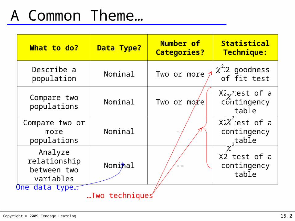
A Common Theme…

What to do? Data Type?Number of

Categories?Statistical Technique:

Describe a population

Nominal Two or moreX2 goodness of

fit test

Compare two populations

Nominal Two or moreX2 test of a contingency

table

Compare two or more populations

Nominal --X2 test of a contingency

table

Analyze relationship between two

variables

Nominal --X2 test of a contingency

table

One data type……Two techniques


Two Techniques…The first is a goodness-of-fit test applied to data produced by a multinomial experiment, a generalization of a binomial experiment and is used to describe one population of data.

The second uses data arranged in a contingency table to determine whether two classifications of a population of nominal data are statistically independent; this test can also be interpreted as a comparison of two or more populations.

In both cases, we use the chi-squared ( ) distribution.


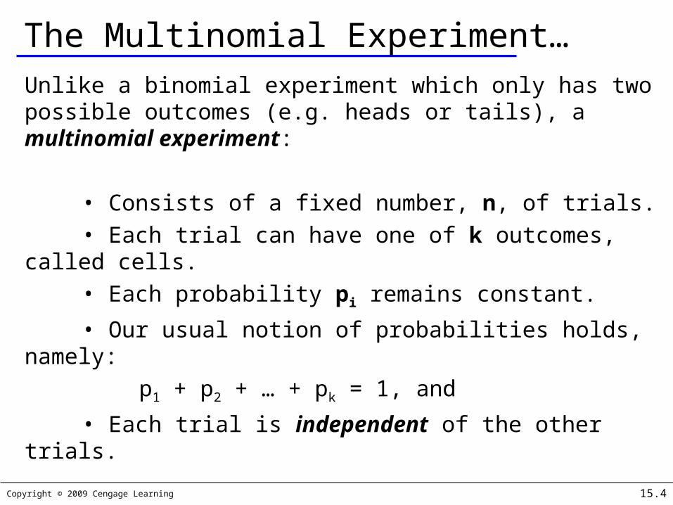
The Multinomial Experiment…Unlike a binomial experiment which only has two possible outcomes (e.g. heads or tails), a multinomial experiment:

• Consists of a fixed number, n, of trials. • Each trial can have one of k outcomes, called cells.

• Each probability pi remains constant.

• Our usual notion of probabilities holds, namely:

p1 + p2 + … + pk = 1, and

• Each trial is independent of the other trials.


Chi-squared Goodness-of-Fit Test…We test whether there is sufficient evidence to reject a specified set of values for pi.

To illustrate, our null hypothesis is:

H0: p1 = a1, p2 = a2, …, pk = ak

where a1, a2, …, ak are the values we want to test.

Our research hypothesis is:H1: At least one pi is not equal to its

specified value


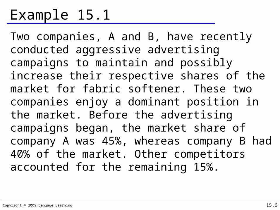
Example 15.1

Two companies, A and B, have recently conducted aggressive advertising campaigns to maintain and possibly increase their respective shares of the market for fabric softener. These two companies enjoy a dominant position in the market. Before the advertising campaigns began, the market share of company A was 45%, whereas company B had 40% of the market. Other competitors accounted for the remaining 15%.


Example 15.1To determine whether these market shares changed after the advertising campaigns, a marketing analyst solicited the preferences of a random sample of 200 customers of fabric softener. Of the 200 customers, 102 indicated a preference for company A's product, 82 preferred company B's fabric softener, and the remaining 16 preferred the products of one of the competitors. Can the analyst infer at the 5% significance level that customer preferences have changed from their levels before the advertising campaigns were launched?


Example 15.1…We compare market share before and after an advertising campaign to see if there is a difference (i.e. if the advertising was effective in improving market share). We hypothesize values for the parameters equal to the before-market share. That is,

H0: p1 = .45, p2 = .40, p3 = .15

The alternative hypothesis is a denial of the null. That is,

H1: At least one pi is not equal to its specified value


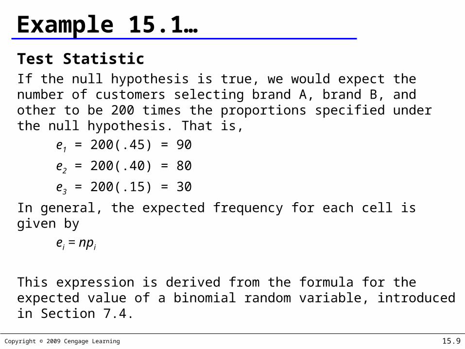
Example 15.1…Test StatisticIf the null hypothesis is true, we would expect the number of customers selecting brand A, brand B, and other to be 200 times the proportions specified under the null hypothesis. That is,

e1 = 200(.45) = 90

e2 = 200(.40) = 80

e3 = 200(.15) = 30

In general, the expected frequency for each cell is given by

ei = npi

This expression is derived from the formula for the expected value of a binomial random variable, introduced in Section 7.4.


Example 15.1…If the expected frequencies and the observed frequencies are quite different, we would conclude that the null hypothesis is false, and we would reject it.

However, if the expected and observed frequencies are similar, we would not reject the null hypothesis.

The test statistic measures the similarity of the expected and observed frequencies.


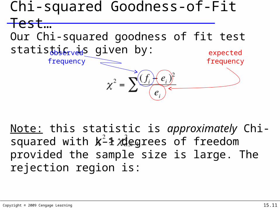
Chi-squared Goodness-of-Fit Test…

Our Chi-squared goodness of fit test statistic is given by:

Note: this statistic is approximately Chi-squared with k–1 degrees of freedom provided the sample size is large. The rejection region is:

observed frequency

expected frequency


Example 15.1…

In order to calculate our test statistic, we lay-out the data in a tabular fashion for easier calculation by hand:

Company

Observed Frequenc

y

Expected Frequenc

yDelta

SummationComponent

fi ei (fi – ei) (fi – ei)2/ei

A 102 90 12 1.60

B 82 80 2 0.05

Others 16 30 -14 6.53

Total 200 200 8.18

Check that these are equal

COMPUTE


Example 15.1…

Our rejection region is:

Since our test statistic is 8.18 which is greater than our critical value for Chi-squared, we reject H0 in favor of H1, that is,

“There is sufficient evidence to infer that the proportions have changed since

the advertising campaigns were implemented”

INTERPRET


Example 15.1… p-value


Required Conditions…

In order to use this technique, the sample size must be large enough so that the expected value for each cell is 5 or more. (i.e. n x pi ≥ 5)

If the expected frequency is less than five, combine it with other cells to satisfy the condition.


Identifying Factors…

Factors that Identify the Chi-Squared Goodness-of-Fit Test:

ei=(n)(pi)


Chi-squared Test of a Contingency TableThe Chi-squared test of a contingency table is used to:

• determine whether there is enough evidence to infer that two nominal variables are related, and

• to infer that differences exist among two or more populations of nominal variables.

In order to use use these techniques, we need to classify the data according to two different criteria.


Example 15.2The MBA program was experiencing problems scheduling their courses. The demand for the program's optional courses and majors was quite variable from one year to the next.

In desperation the dean of the business school turned to a statistics professor for assistance.

The statistics professor believed that the problem may be the variability in the academic background of the students and that the undergraduate degree affects the choice of major.


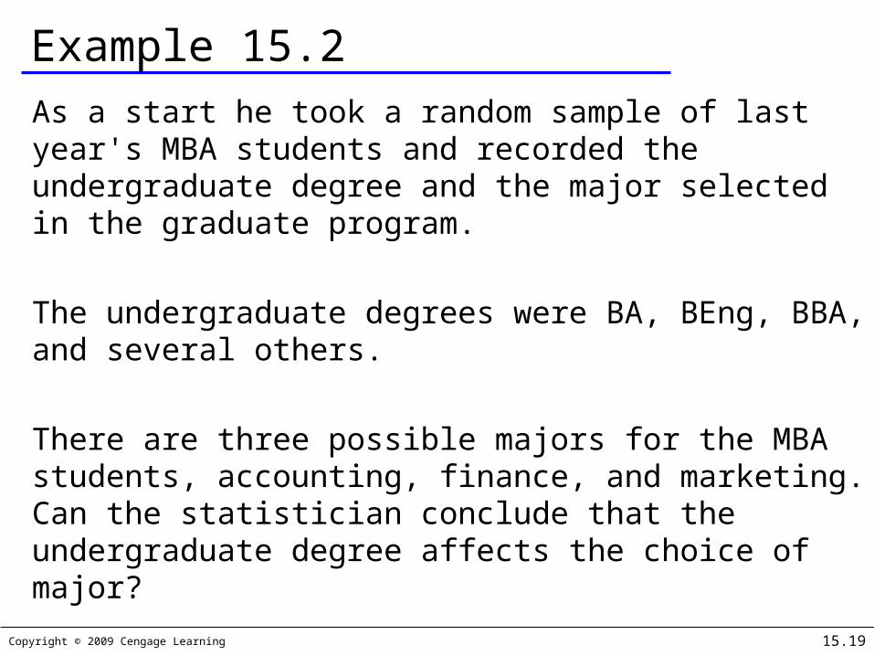
Example 15.2As a start he took a random sample of last year's MBA students and recorded the undergraduate degree and the major selected in the graduate program.

The undergraduate degrees were BA, BEng, BBA, and several others.

There are three possible majors for the MBA students, accounting, finance, and marketing. Can the statistician conclude that the undergraduate degree affects the choice of major?


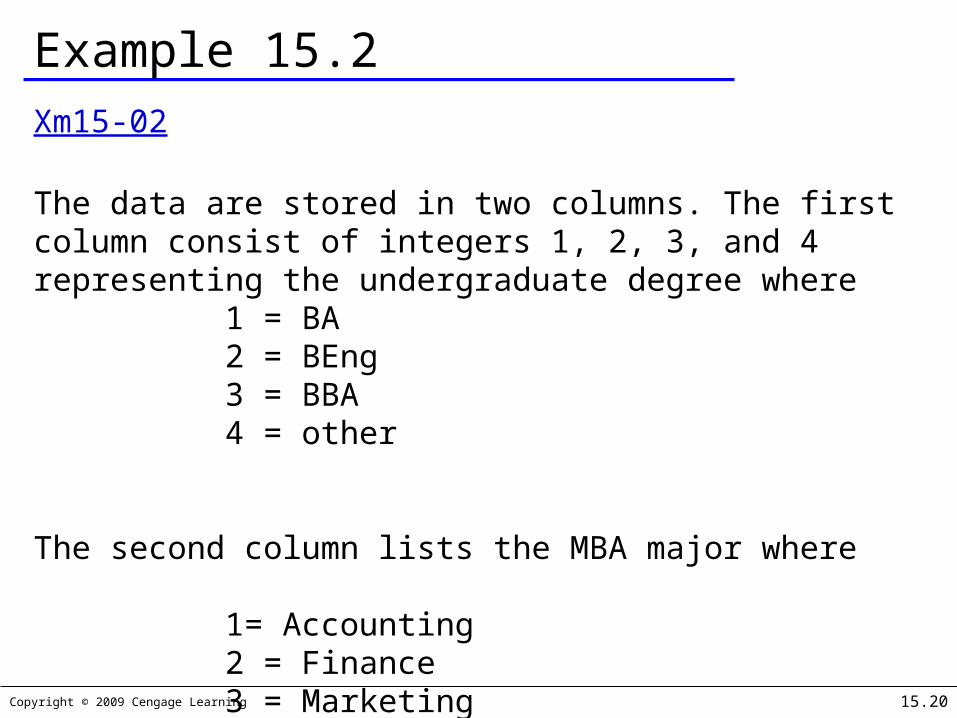
Example 15.2Xm15-02

The data are stored in two columns. The first column consist of integers 1, 2, 3, and 4 representing the undergraduate degree where

1 = BA2 = BEng3 = BBA4 = other

The second column lists the MBA major where

1= Accounting2 = Finance3 = Marketing


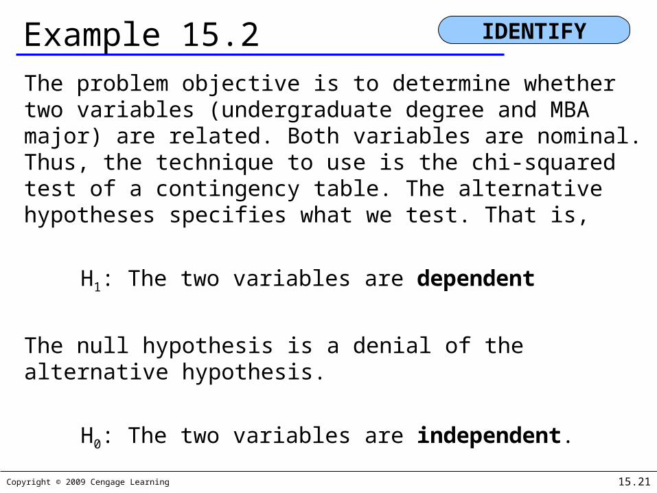
Example 15.2The problem objective is to determine whether two variables (undergraduate degree and MBA major) are related. Both variables are nominal. Thus, the technique to use is the chi-squared test of a contingency table. The alternative hypotheses specifies what we test. That is,

H1: The two variables are dependent

The null hypothesis is a denial of the alternative hypothesis.

H0: The two variables are independent.

IDENTIFY


Test StatisticThe test statistic is the same as the one used to test proportions in the goodness-of-fit-test. That is, the test statistic is

Note however, that there is a major difference between the two applications. In this one the null does not specify the proportions pi, from which we compute the expected values ei, which we need to calculate the χ2 test statistic. That is, we cannot use

e = npi

because we don’t know the pi (they are not specified by the null hypothesis). It is necessary to estimate the pi from the data.

i

ii

e

ef 22 )(


Example 15.2

The first step is to count the number of students in each of the 12 combinations. The result is called a cross-classification table.


Example 15.2

MBA Major

Undergrad Degree

Accounting

Finance Marketing Total

BA 31 13 16 60

BEng 8 16 7 31

BBA 12 10 17 39

Other 10 5 7 22

Total 61 44 47 152


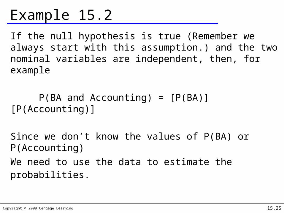
Example 15.2If the null hypothesis is true (Remember we always start with this assumption.) and the two nominal variables are independent, then, for example

P(BA and Accounting) = [P(BA)] [P(Accounting)]

Since we don’t know the values of P(BA) or P(Accounting)

We need to use the data to estimate the probabilities.


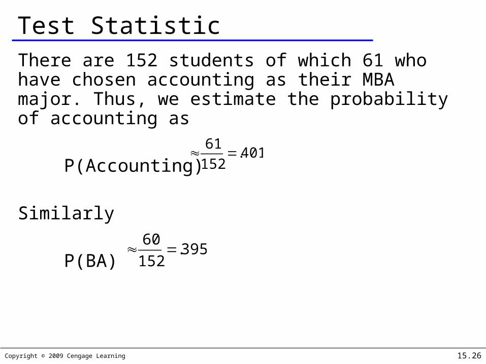
Test StatisticThere are 152 students of which 61 who have chosen accounting as their MBA major. Thus, we estimate the probability of accounting as

P(Accounting)

Similarly

P(BA)

401.152

61

395.152

60


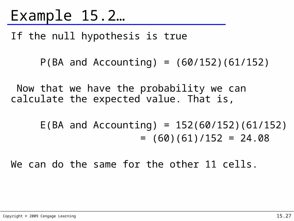
Example 15.2…If the null hypothesis is true

P(BA and Accounting) = (60/152)(61/152)

Now that we have the probability we can calculate the expected value. That is,

E(BA and Accounting) = 152(60/152)(61/152) = (60)(61)/152 = 24.08

We can do the same for the other 11 cells.


Example 15.2

We can now compare observed with expected frequencies…

and calculate our test statistic:

MBA Major

Undergrad Degree

Accounting Finance Marketing

BA 31 24.08 13 17.37 16 18.55

BEng 8 12.44 16 8.97 7 9.59

BBA 12 15.65 10 11.29 17 12.06

Other 10 8.83 5 6.37 7 6.80

COMPUTE


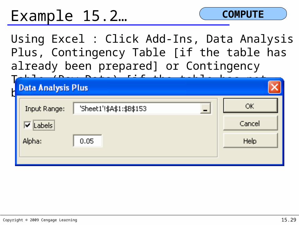
Example 15.2…Using Excel : Click Add-Ins, Data Analysis Plus, Contingency Table [if the table has already been prepared] or Contingency Table (Raw Data) [if the table has not been completed]

COMPUTE


Example 15.2… COMPUTE

123456789101112131415

A B C D E FContingency Table

DegreeMBA Major 1 2 3 TOTAL

1 31 13 16 602 8 16 7 313 12 10 17 394 10 5 7 22

TOTAL 61 44 47 152

chi-squared Stat 14.7019df 6p-value 0.0227chi-squared Critical 12.5916

The printout below was produced from file Xm15-02 using the Contingency Table (Raw Data) command


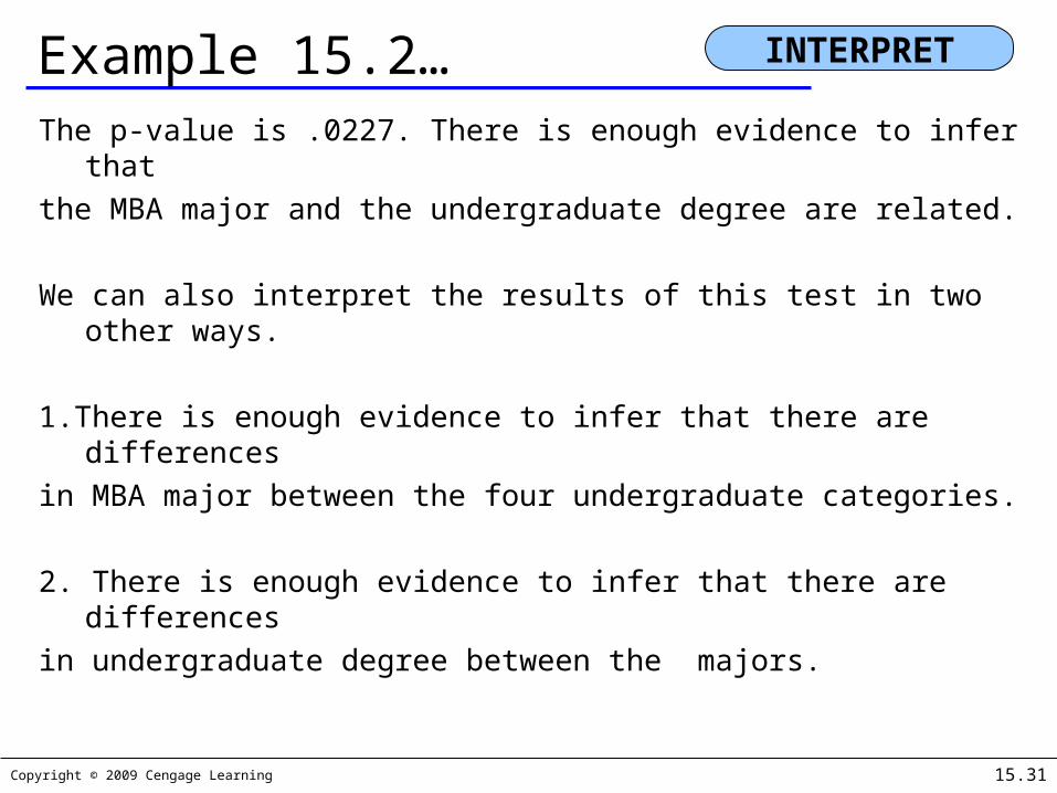
Example 15.2…The p-value is .0227. There is enough evidence to infer

thatthe MBA major and the undergraduate degree are related.

We can also interpret the results of this test in two other ways.

1.There is enough evidence to infer that there are differences

in MBA major between the four undergraduate categories.

2. There is enough evidence to infer that there are differences

in undergraduate degree between the majors.

INTERPRET


Required Condition – Rule of Five…

In a contingency table where one or more cells have expected values of less than 5, we need to combine rows or columns to satisfy the rule of five.

Note: by doing this, the degrees of freedom must be changed as well.


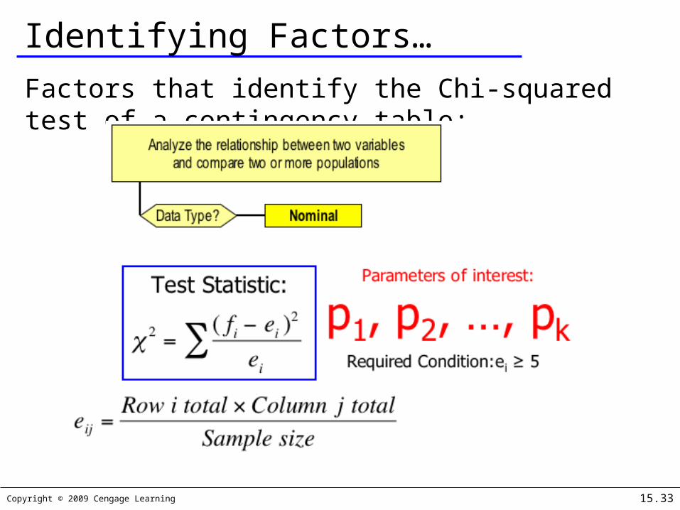
Identifying Factors…

Factors that identify the Chi-squared test of a contingency table:


Table 15.1 Statistical Techniques for Nominal DataProblem Objective Categories Statistical TechniqueDescribe a population 2 z-test of p or the chi-squared

goodness-of-fit test

Describe a population More than 2 Chi-squared goodness-of-fit test

Compare two populations 2 z-test p1–p2 or chi-squared test

of a contingency table

Compare two populations More than 2 Chi-squared test of a contingency table

Compare more thantwo populations 2 or more Chi-squared test of a contingency table Analyze the relationship between two variables 2 or more Chi-squared test of a contingency table

Copyright © 2009 Cengage Learning 15.1 Chapter 16 Chi-Squared Tests.

Documents

Transcript of Copyright © 2009 Cengage Learning 15.1 Chapter 16 Chi-Squared Tests.