
Controls for Lathes Programmer's Manual - NCT
228
NCT ® 99T NCT ® 2000T Controls for Lathes Programmer's Manual
Transcript of Controls for Lathes Programmer's Manual - NCT

NCT® 99T
NCT® 2000TControls for Lathes
Programmer's Manual

Manufactured by NCT Automation kft.H1148 Budapest Fogarasi út 7: Address: H1631 Bp. pf.: 26F Phone: (+36 1) 467 63 00F Fax:(+36 1) 363 6605
E-mail: [email protected] Page: www.nct.hu

3
Contents
1 Introduction . . . . . . . . . . . . . . . . . . . . . . . . . . . . . . . . . . . . . . . . . . . . . . . . . . . . . . . . . . . . . . 91.1 The Part Program . . . . . . . . . . . . . . . . . . . . . . . . . . . . . . . . . . . . . . . . . . . . . . . . . . . . . . 9
Word . . . . . . . . . . . . . . . . . . . . . . . . . . . . . . . . . . . . . . . . . . . . . . . . . . . . . . . . . . . . . . . 9Address Chain . . . . . . . . . . . . . . . . . . . . . . . . . . . . . . . . . . . . . . . . . . . . . . . . . . . . . . . . . 9Block . . . . . . . . . . . . . . . . . . . . . . . . . . . . . . . . . . . . . . . . . . . . . . . . . . . . . . . . . . . . . . 10Program Number and Program Name . . . . . . . . . . . . . . . . . . . . . . . . . . . . . . . . . . . . . . 10Beginning of Program, End of Program . . . . . . . . . . . . . . . . . . . . . . . . . . . . . . . . . . . . . . 10Program Format in the Memory . . . . . . . . . . . . . . . . . . . . . . . . . . . . . . . . . . . . . . . . . . . 10Program Format in Communications with External Devices . . . . . . . . . . . . . . . . . . . . . . . 10Main Program and Sub-program . . . . . . . . . . . . . . . . . . . . . . . . . . . . . . . . . . . . . . . . . . 10DNC Channel . . . . . . . . . . . . . . . . . . . . . . . . . . . . . . . . . . . . . . . . . . . . . . . . . . . . . . . . 11
1.2 Fundamental Terms . . . . . . . . . . . . . . . . . . . . . . . . . . . . . . . . . . . . . . . . . . . . . . . . . . . . 12
2 Controlled Axes . . . . . . . . . . . . . . . . . . . . . . . . . . . . . . . . . . . . . . . . . . . . . . . . . . . . . . . . . 172.1 Names of Axes . . . . . . . . . . . . . . . . . . . . . . . . . . . . . . . . . . . . . . . . . . . . . . . . . . . . . . . 172.2 Unit and Increment System of Axes . . . . . . . . . . . . . . . . . . . . . . . . . . . . . . . . . . . . . . . . 17
3 Preparatory Functions (G codes) . . . . . . . . . . . . . . . . . . . . . . . . . . . . . . . . . . . . . . . . . . . . 19
4 The Interpolation . . . . . . . . . . . . . . . . . . . . . . . . . . . . . . . . . . . . . . . . . . . . . . . . . . . . . . . . 234.1 Positioning (G00) . . . . . . . . . . . . . . . . . . . . . . . . . . . . . . . . . . . . . . . . . . . . . . . . . . . . . 234.2 Linear Interpolation (G01) . . . . . . . . . . . . . . . . . . . . . . . . . . . . . . . . . . . . . . . . . . . . . . . 234.3 Circular and Spiral Interpolation (G02, G03) . . . . . . . . . . . . . . . . . . . . . . . . . . . . . . . . . 254.4 Equal Lead Thread Cutting (G33) . . . . . . . . . . . . . . . . . . . . . . . . . . . . . . . . . . . . . . . . . 294.5 Variable-Lead Thread Cutting (G34) . . . . . . . . . . . . . . . . . . . . . . . . . . . . . . . . . . . . . . . 304.6 Polar Coordinate Interpolation (G12.1, G13.1) . . . . . . . . . . . . . . . . . . . . . . . . . . . . . . . 314.7 Cylindrical Interpolation (G7.1) . . . . . . . . . . . . . . . . . . . . . . . . . . . . . . . . . . . . . . . . . . . 35
5 The Coordinate Data . . . . . . . . . . . . . . . . . . . . . . . . . . . . . . . . . . . . . . . . . . . . . . . . . . . . . 385.1 Absolute and Incremental Programming (G90, G91), Operator I . . . . . . . . . . . . . . . . . . 385.2 Inch/Metric Conversion (G20, G21) . . . . . . . . . . . . . . . . . . . . . . . . . . . . . . . . . . . . . . . 385.3 Specification and Value Range of Coordinate Data . . . . . . . . . . . . . . . . . . . . . . . . . . . . 395.4 Programming in Radius or Diameter . . . . . . . . . . . . . . . . . . . . . . . . . . . . . . . . . . . . . . . . 405.5 Rotary Axis Roll-over . . . . . . . . . . . . . . . . . . . . . . . . . . . . . . . . . . . . . . . . . . . . . . . . . . 41
6 The Feed . . . . . . . . . . . . . . . . . . . . . . . . . . . . . . . . . . . . . . . . . . . . . . . . . . . . . . . . . . . . . . . 446.1 Feed in Rapid Travers . . . . . . . . . . . . . . . . . . . . . . . . . . . . . . . . . . . . . . . . . . . . . . . . . . 446.2 Cutting Feed Rate . . . . . . . . . . . . . . . . . . . . . . . . . . . . . . . . . . . . . . . . . . . . . . . . . . . . . 44
6.2.1 Feed per Minute (G94) and Feed per Revolution (G95) . . . . . . . . . . . . . . . . . . . . 456.2.2 Clamping the Cutting Feed . . . . . . . . . . . . . . . . . . . . . . . . . . . . . . . . . . . . . . . . . . 46
6.3 Automatic Acceleration/Deceleration . . . . . . . . . . . . . . . . . . . . . . . . . . . . . . . . . . . . . . . 476.4 Feed Control Functions . . . . . . . . . . . . . . . . . . . . . . . . . . . . . . . . . . . . . . . . . . . . . . . . . 48
6.4.1 Exact Stop (G09) . . . . . . . . . . . . . . . . . . . . . . . . . . . . . . . . . . . . . . . . . . . . . . . . . 48

4
6.4.2 Exact Stop Mode (G61) . . . . . . . . . . . . . . . . . . . . . . . . . . . . . . . . . . . . . . . . . . . 486.4.3 Continuous Cutting Mode (G64) . . . . . . . . . . . . . . . . . . . . . . . . . . . . . . . . . . . . . 496.4.4 Override and Stop Inhibit (Tapping) Mode (G63) . . . . . . . . . . . . . . . . . . . . . . . . 496.4.5 Automatic Corner Override (G62) . . . . . . . . . . . . . . . . . . . . . . . . . . . . . . . . . . . . 496.4.6 Internal Circular Cutting Override . . . . . . . . . . . . . . . . . . . . . . . . . . . . . . . . . . . . . 50
7 The Dwell (G04) . . . . . . . . . . . . . . . . . . . . . . . . . . . . . . . . . . . . . . . . . . . . . . . . . . . . . . . . . 51
8 The Reference Point . . . . . . . . . . . . . . . . . . . . . . . . . . . . . . . . . . . . . . . . . . . . . . . . . . . . . 528.1 Automatic Reference Point Return (G28) . . . . . . . . . . . . . . . . . . . . . . . . . . . . . . . . . . . 528.2 Automatic Return to Reference Points 2, 3, 4 (G30) . . . . . . . . . . . . . . . . . . . . . . . . . . . 538.3 Automatic Return from the Reference Point (G29) . . . . . . . . . . . . . . . . . . . . . . . . . . . . . 53
9 Coordinate Systems, Plane Selection . . . . . . . . . . . . . . . . . . . . . . . . . . . . . . . . . . . . . . . . 559.1 The Machine Coordinate System . . . . . . . . . . . . . . . . . . . . . . . . . . . . . . . . . . . . . . . . . 55
9.1.1 Setting the Machine Coordinate System . . . . . . . . . . . . . . . . . . . . . . . . . . . . . . . . 559.1.2 Positioning in the Machine Coordinate System (G53) . . . . . . . . . . . . . . . . . . . . . . 56
9.2 Work Coordinate Systems . . . . . . . . . . . . . . . . . . . . . . . . . . . . . . . . . . . . . . . . . . . . . . 569.2.1 Setting the Work Coordinate Systems . . . . . . . . . . . . . . . . . . . . . . . . . . . . . . . . . 569.2.2 Selecting the Work Coordinate System . . . . . . . . . . . . . . . . . . . . . . . . . . . . . . . . 579.2.3 Programmed Setting of the Work Zero Point Offset . . . . . . . . . . . . . . . . . . . . . . . 589.2.4 Creating a New Work Coordinate System (G92) . . . . . . . . . . . . . . . . . . . . . . . . . 59
9.3 Local Coordinate System . . . . . . . . . . . . . . . . . . . . . . . . . . . . . . . . . . . . . . . . . . . . . . . 609.4 Plane Selection (G17, G18, G19) . . . . . . . . . . . . . . . . . . . . . . . . . . . . . . . . . . . . . . . . . 61
10 The Spindle Function . . . . . . . . . . . . . . . . . . . . . . . . . . . . . . . . . . . . . . . . . . . . . . . . . . . . 6310.1 Spindle Speed Command (code S) . . . . . . . . . . . . . . . . . . . . . . . . . . . . . . . . . . . . . . . 6310.2 Programming of Constant Surface Speed Control . . . . . . . . . . . . . . . . . . . . . . . . . . . . 63
10.2.1Constant Surface Speed Control Command (G96, G97) . . . . . . . . . . . . . . . . . . . 6410.2.2 Constant Surface Speed Clamp (G92) . . . . . . . . . . . . . . . . . . . . . . . . . . . . . . . . 6410.2.3 Selecting an Axis for Constant Surface Speed Control . . . . . . . . . . . . . . . . . . . . 65
10.3 Spindle Position Feedback . . . . . . . . . . . . . . . . . . . . . . . . . . . . . . . . . . . . . . . . . . . . . 6510.4 Oriented Spindle Stop . . . . . . . . . . . . . . . . . . . . . . . . . . . . . . . . . . . . . . . . . . . . . . . . 6510.5 Spindle Positioning (Indexing) . . . . . . . . . . . . . . . . . . . . . . . . . . . . . . . . . . . . . . . . . . . 6610.6 Spindle Speed Fluctuation Detection (G25, G26) . . . . . . . . . . . . . . . . . . . . . . . . . . . . 66
11 Tool Function . . . . . . . . . . . . . . . . . . . . . . . . . . . . . . . . . . . . . . . . . . . . . . . . . . . . . . . . . . 69
12 Miscellaneous and Auxiliary Functions . . . . . . . . . . . . . . . . . . . . . . . . . . . . . . . . . . . . . 7012.1 Miscellaneous Functions (Codes M) . . . . . . . . . . . . . . . . . . . . . . . . . . . . . . . . . . . . . . 7012.2 Auxiliary Function (Codes A, B, C) . . . . . . . . . . . . . . . . . . . . . . . . . . . . . . . . . . . . . . 7112.3 Sequence of Execution of Various Functions . . . . . . . . . . . . . . . . . . . . . . . . . . . . . . . . 71
13 Part Program Configuration . . . . . . . . . . . . . . . . . . . . . . . . . . . . . . . . . . . . . . . . . . . . . . . 7213.1 Sequence Number (Address N) . . . . . . . . . . . . . . . . . . . . . . . . . . . . . . . . . . . . . . . . . 7213.2 Conditional Block Skip . . . . . . . . . . . . . . . . . . . . . . . . . . . . . . . . . . . . . . . . . . . . . . . . 72

5
13.3 Main Program and Sub-program . . . . . . . . . . . . . . . . . . . . . . . . . . . . . . . . . . . . . . . . . 7213.3.1 Calling the Sub-program . . . . . . . . . . . . . . . . . . . . . . . . . . . . . . . . . . . . . . . . . . . 7213.3.2 Return from a Sub-program . . . . . . . . . . . . . . . . . . . . . . . . . . . . . . . . . . . . . . . . 7313.3.3 Jump within the Main Program . . . . . . . . . . . . . . . . . . . . . . . . . . . . . . . . . . . . . . 75
14 The Tool Compensation . . . . . . . . . . . . . . . . . . . . . . . . . . . . . . . . . . . . . . . . . . . . . . . . . . 7614.1 Reference to Tool Offset . . . . . . . . . . . . . . . . . . . . . . . . . . . . . . . . . . . . . . . . . . . . . . . 7614.2 Modification of Tool Offset Values from the Program (G10) . . . . . . . . . . . . . . . . . . . . 8014.3 Taking the Tool Length Offset into Account . . . . . . . . . . . . . . . . . . . . . . . . . . . . . . . . . 8014.4 Tool Nose Radius Compensation (G38, G39, G40, G41, G42) . . . . . . . . . . . . . . . . . . 82
14.4.1 Start up of Tool Nose Radius Compensation . . . . . . . . . . . . . . . . . . . . . . . . . . . . 8614.4.2 Rules of Tool Nose Radius Compensation in Offset Mode . . . . . . . . . . . . . . . . . . 9014.4.3 Canceling of Offset Mode . . . . . . . . . . . . . . . . . . . . . . . . . . . . . . . . . . . . . . . . . . 9314.4.4 Change of Offset Direction While in the Offset Mode . . . . . . . . . . . . . . . . . . . . . 9614.4.5 Programming Vector Hold (G38) . . . . . . . . . . . . . . . . . . . . . . . . . . . . . . . . . . . . 9814.4.6 Programming Corner Arcs (G39) . . . . . . . . . . . . . . . . . . . . . . . . . . . . . . . . . . . . 9814.4.7 General Information on Tool Nose Radius Compensation . . . . . . . . . . . . . . . . . 10014.4.8 Interferences in Tool Nose Radius Compensation . . . . . . . . . . . . . . . . . . . . . . . 105
15 Special Transformations . . . . . . . . . . . . . . . . . . . . . . . . . . . . . . . . . . . . . . . . . . . . . . . . . 11015.1 Mirror Image for Double Turret (G68) . . . . . . . . . . . . . . . . . . . . . . . . . . . . . . . . . . . . 11015.2 Scaling (G50, G51) . . . . . . . . . . . . . . . . . . . . . . . . . . . . . . . . . . . . . . . . . . . . . . . . . . 11115.3 Programmable Mirror Image (G50.1, G51.1) . . . . . . . . . . . . . . . . . . . . . . . . . . . . . . 111
16 Automatic Geometric Calculations . . . . . . . . . . . . . . . . . . . . . . . . . . . . . . . . . . . . . . . . 11416.1 Programming Chamfer and Corner Round . . . . . . . . . . . . . . . . . . . . . . . . . . . . . . . . . 11416.2 Specifying Straight Line with Angle . . . . . . . . . . . . . . . . . . . . . . . . . . . . . . . . . . . . . . 11516.3 Intersection Calculations in the Selected Plane . . . . . . . . . . . . . . . . . . . . . . . . . . . . . . 117
16.3.1 Linear-linear Intersection . . . . . . . . . . . . . . . . . . . . . . . . . . . . . . . . . . . . . . . . . . 11716.3.2 Linear-circular Intersection . . . . . . . . . . . . . . . . . . . . . . . . . . . . . . . . . . . . . . . . 11916.3.3 Circular-linear Intersection . . . . . . . . . . . . . . . . . . . . . . . . . . . . . . . . . . . . . . . . 12116.3.4 Circular-circular Intersection . . . . . . . . . . . . . . . . . . . . . . . . . . . . . . . . . . . . . . . 12316.3.5 Chaining of Intersection Calculations . . . . . . . . . . . . . . . . . . . . . . . . . . . . . . . . . 125
17 Canned Cycles for Turning . . . . . . . . . . . . . . . . . . . . . . . . . . . . . . . . . . . . . . . . . . . . . . . 12617.1 Single Cycles . . . . . . . . . . . . . . . . . . . . . . . . . . . . . . . . . . . . . . . . . . . . . . . . . . . . . . 126
17.1.1 Cutting Cycle (G77) . . . . . . . . . . . . . . . . . . . . . . . . . . . . . . . . . . . . . . . . . . . . . 12617.1.2 Thread Cutting Cycle (G78) . . . . . . . . . . . . . . . . . . . . . . . . . . . . . . . . . . . . . . . 12817.1.3 End Face Cutting Cycle (G79) . . . . . . . . . . . . . . . . . . . . . . . . . . . . . . . . . . . . . 13017.1.4 Single Cycle Application . . . . . . . . . . . . . . . . . . . . . . . . . . . . . . . . . . . . . . . . . . 132
17.2 Multiple Repetitive Cycles . . . . . . . . . . . . . . . . . . . . . . . . . . . . . . . . . . . . . . . . . . . . . 13317.2.1 Stock Removal in Turning (G71) . . . . . . . . . . . . . . . . . . . . . . . . . . . . . . . . . . . . 13317.2.2 Stock Removal in Facing (G72) . . . . . . . . . . . . . . . . . . . . . . . . . . . . . . . . . . . . 13817.2.3 Pattern Repeating Cycle (G73) . . . . . . . . . . . . . . . . . . . . . . . . . . . . . . . . . . . . . 14017.2.4 Finishing Cycle (G70) . . . . . . . . . . . . . . . . . . . . . . . . . . . . . . . . . . . . . . . . . . . . 14217.2.5 End Face Peck Drilling Cycle (G74) . . . . . . . . . . . . . . . . . . . . . . . . . . . . . . . . . 143

6
17.2.6 Outer Diameter/Internal Diameter Drilling Cycle (G75) . . . . . . . . . . . . . . . . . . . 14517.2.7 Multiple Thread Cutting Cycle (G76) . . . . . . . . . . . . . . . . . . . . . . . . . . . . . . . . 146
18 Canned Cycles for Drilling . . . . . . . . . . . . . . . . . . . . . . . . . . . . . . . . . . . . . . . . . . . . . . 15218.1 Detailed Description of Canned Cycles . . . . . . . . . . . . . . . . . . . . . . . . . . . . . . . . . . . 158
18.1.1 High Speed Peck Drilling Cycle (G83.1) . . . . . . . . . . . . . . . . . . . . . . . . . . . . . 15818.1.2 Counter Tapping Cycle (G84.1) . . . . . . . . . . . . . . . . . . . . . . . . . . . . . . . . . . . . 15918.1.3 Fine Boring Cycle (G86.1) . . . . . . . . . . . . . . . . . . . . . . . . . . . . . . . . . . . . . . . . 16018.1.4 Canned Cycle for Drilling Cancel (G80) . . . . . . . . . . . . . . . . . . . . . . . . . . . . . . 16118.1.5 Drilling, Spot Boring Cycle (G81) . . . . . . . . . . . . . . . . . . . . . . . . . . . . . . . . . . . 16118.1.6 Drilling, Counter Boring Cycle (G82) . . . . . . . . . . . . . . . . . . . . . . . . . . . . . . . . 16218.1.7 Peck Drilling Cycle (G83) . . . . . . . . . . . . . . . . . . . . . . . . . . . . . . . . . . . . . . . . 16318.1.8 Tapping Cycle (G84) . . . . . . . . . . . . . . . . . . . . . . . . . . . . . . . . . . . . . . . . . . . . 16418.1.9 Rigid (Clockwise and Counter-clockwise) Tap Cycles (G84.2, G84.3) . . . . . . . 16518.1.10 Boring Cycle (G85) . . . . . . . . . . . . . . . . . . . . . . . . . . . . . . . . . . . . . . . . . . . . 16818.1.11 Boring Cycle Tool Retraction with Rapid Traverse (G86) . . . . . . . . . . . . . . . . 16918.1.12 Boring Cycle/Back Boring Cycle (G87) . . . . . . . . . . . . . . . . . . . . . . . . . . . . . 17018.1.13 Boring Cycle (Manual Operation on the Bottom Point) (G88) . . . . . . . . . . . . . 17218.1.14 Boring Cycle (Dwell on the Bottom Point, Retraction with Feed) (G89) . . . . . 173
18.2 Notes to the Use of Canned Cycles for Drilling . . . . . . . . . . . . . . . . . . . . . . . . . . . . . 173
19 Polygonal Turning . . . . . . . . . . . . . . . . . . . . . . . . . . . . . . . . . . . . . . . . . . . . . . . . . . . . . 17519.1 Principle of Polygonal Turning . . . . . . . . . . . . . . . . . . . . . . . . . . . . . . . . . . . . . . . . . . 17519.2 Programming Polygonal Turning (G51.2, G50.2) . . . . . . . . . . . . . . . . . . . . . . . . . . . . 176
20 Measurement Functions . . . . . . . . . . . . . . . . . . . . . . . . . . . . . . . . . . . . . . . . . . . . . . . . 17820.1 Skip Function (G31) . . . . . . . . . . . . . . . . . . . . . . . . . . . . . . . . . . . . . . . . . . . . . . . . . 17820.2 Automatic Tool Length Measurement (G36, G37) . . . . . . . . . . . . . . . . . . . . . . . . . . . 179
21 Safety Functions . . . . . . . . . . . . . . . . . . . . . . . . . . . . . . . . . . . . . . . . . . . . . . . . . . . . . . . 18121.1 Programmable Stroke Check (G22, G23) . . . . . . . . . . . . . . . . . . . . . . . . . . . . . . . . . 18121.2 Parametric Overtravel Positions . . . . . . . . . . . . . . . . . . . . . . . . . . . . . . . . . . . . . . . . 18221.3 Stroke Check Before Movement . . . . . . . . . . . . . . . . . . . . . . . . . . . . . . . . . . . . . . . 183
22 Custom Macro . . . . . . . . . . . . . . . . . . . . . . . . . . . . . . . . . . . . . . . . . . . . . . . . . . . . . . . . 18422.1 The Simple Macro Call (G65) . . . . . . . . . . . . . . . . . . . . . . . . . . . . . . . . . . . . . . . . . 18422.2 The Macro Modal Call . . . . . . . . . . . . . . . . . . . . . . . . . . . . . . . . . . . . . . . . . . . . . . . 185
22.2.1 Macro Modal Call in Every Motion Command (G66) . . . . . . . . . . . . . . . . . . . . 18522.2.2 Macro Modal Call From Each Block (G66.1) . . . . . . . . . . . . . . . . . . . . . . . . . 186
22.3 Custom Macro Call Using G Code . . . . . . . . . . . . . . . . . . . . . . . . . . . . . . . . . . . . . . 18722.4 Custom Macro Call Using M Code . . . . . . . . . . . . . . . . . . . . . . . . . . . . . . . . . . . . . 18822.5 Subprogram Call with M Code . . . . . . . . . . . . . . . . . . . . . . . . . . . . . . . . . . . . . . . . . 18822.6 Subprogram Call with T Code . . . . . . . . . . . . . . . . . . . . . . . . . . . . . . . . . . . . . . . . . 18922.7 Subprogram Call with S Code . . . . . . . . . . . . . . . . . . . . . . . . . . . . . . . . . . . . . . . . . 18922.8 Subprogram Call with A, B, C Codes . . . . . . . . . . . . . . . . . . . . . . . . . . . . . . . . . . . . 18922.9 Differences Between the Call of a Sub-Program and the Call of a Macro . . . . . . . . . . 190
7
22.9.1 Multiple Calls . . . . . . . . . . . . . . . . . . . . . . . . . . . . . . . . . . . . . . . . . . . . . . . . . . 19022.10 Format of Custom Macro Body . . . . . . . . . . . . . . . . . . . . . . . . . . . . . . . . . . . . . . . 19122.11 Variables of the Programming Language . . . . . . . . . . . . . . . . . . . . . . . . . . . . . . . . . 192
22.11.1 Identification of a Variable . . . . . . . . . . . . . . . . . . . . . . . . . . . . . . . . . . . . . . . 19222.11.2 Referring to a Variable . . . . . . . . . . . . . . . . . . . . . . . . . . . . . . . . . . . . . . . . . . 19222.11.3 Vacant Variables . . . . . . . . . . . . . . . . . . . . . . . . . . . . . . . . . . . . . . . . . . . . . . 19322.11.4 Numerical Format of Variables . . . . . . . . . . . . . . . . . . . . . . . . . . . . . . . . . . . . 193
22.12 Types of Variables . . . . . . . . . . . . . . . . . . . . . . . . . . . . . . . . . . . . . . . . . . . . . . . . . 19422.12.1 Local Variables . . . . . . . . . . . . . . . . . . . . . . . . . . . . . . . . . . . . . . . . . . . . . . . 19422.12.2 Common Variables . . . . . . . . . . . . . . . . . . . . . . . . . . . . . . . . . . . . . . . . . . . . 19422.12.3 System Variables . . . . . . . . . . . . . . . . . . . . . . . . . . . . . . . . . . . . . . . . . . . . . . 195
22.13 Instructions of the Programming Language . . . . . . . . . . . . . . . . . . . . . . . . . . . . . . . . 20422.13.1 Definition, Substitution . . . . . . . . . . . . . . . . . . . . . . . . . . . . . . . . . . . . . . . . . . 20422.13.2 Arithmetic Operations and Functions . . . . . . . . . . . . . . . . . . . . . . . . . . . . . . . . 20422.13.3 Logical Operations . . . . . . . . . . . . . . . . . . . . . . . . . . . . . . . . . . . . . . . . . . . . . 20822.13.4 Unconditional Divergence . . . . . . . . . . . . . . . . . . . . . . . . . . . . . . . . . . . . . . . . 20822.13.5 Conditional Divergence . . . . . . . . . . . . . . . . . . . . . . . . . . . . . . . . . . . . . . . . . . 20822.13.6 Conditional Instruction . . . . . . . . . . . . . . . . . . . . . . . . . . . . . . . . . . . . . . . . . . 20822.13.7 Iteration . . . . . . . . . . . . . . . . . . . . . . . . . . . . . . . . . . . . . . . . . . . . . . . . . . . . . 20922.13.8 Data Output Commands . . . . . . . . . . . . . . . . . . . . . . . . . . . . . . . . . . . . . . . . . 211
22.14 NC and Macro Instructions . . . . . . . . . . . . . . . . . . . . . . . . . . . . . . . . . . . . . . . . . . . 21522.15 Execution of NC and Macro Instructions in Time . . . . . . . . . . . . . . . . . . . . . . . . . . . 21522.16 Displaying Macros and Sub-programs in Automatic Mode . . . . . . . . . . . . . . . . . . . . 21622.17 Using the STOP Button While a Macro Instruction is Being Executed . . . . . . . . . . . . 216
Notes . . . . . . . . . . . . . . . . . . . . . . . . . . . . . . . . . . . . . . . . . . . . . . . . . . . . . . . . . . . . . . . . . . 217
Index in Alphabetical Order . . . . . . . . . . . . . . . . . . . . . . . . . . . . . . . . . . . . . . . . . . . . . . . . 218
July 2, 2002

8
© Copyright NCT July 2, 2002
The Publisher reserves all rights for contentsof this Manual. No reprinting, even inextracts, is permissible unless our writtenconsent is obtained.The text of this Manual has been compiledand checked with utmost care, yet weassume no liability for possible errors orspurious data and for consequential losses ordemages.

1 Introduction
9
1 Introduction
1.1 The Part Program
The Part Program is a set of instructions that can be interpreted by the control system in order tocontrol the operation of the machine.The Part Program consists of blocks which, in turn, comprise words.
Word: Address and DataEach word is made up of two parts - an address and a data. The address has one or morecharacters, the data is a numerical value (an integer or decimal value). Some addresses may be givena sign or operator I.
Address Chain:
Address Meaning Value limits
O program number 0001 - 9999
/ optional block 1 - 9
N block number 1 - 99999
G preparatory function *
X, Y, Z, U, V ,W length coordinates I, -, *
A, B, C, H angular coordinates, auxiliary functions I, -, *
R circle radius, auxiliary data I, -, *
I, J, K circle center coordinates, auxiliary coordinate -, *
E auxiliary coordinate -, *
F feed rate *
S spindle speed *
M miscellaneous function 1 - 999
T tool number 1 - 9999
L repetition number 1 - 9999
P auxiliary data, dwell time -, *
Q auxiliary data -, *
,C distance of chamfer -, *
,R radius of fillet -, *
,A angle of straight line -, *
( comment *
At an address marked with a * in the Value Limits column, the data may have a decimal value aswell.At an address marked with I and –, an incremental operator or a sign can be assigned, respectively.The positive sign + is not indicated and not stored.

1 Introduction
10
BlockA block is made up of words.The blocks are separated by characters s (Line Feed) in the memory. The use of a block numberis not mandatory in the blocks. To distinguish the end of block from the beginning of another blockon the screen, each new block begins in a new line, with a character > placed in front of it, in thecase of a block longer than a line, the words in each new line are begun with an indent of onecharacter.
Program Number and Program NameThe program number and the program name are used for the identification of a program. The use ofprogram number is mandatory that of a program name is not.The address of a program number is O. It must be followed by exactly four digits.The program name is any arbitrary character sequence (string) put between opening "(" andclosing brackets ")". It may have max. 16 characters.The program number and the program name are separated by characters s (Line Feed) from theother program blocks in the memory.In the course of editing, the program number and the program name will be displayed invariably inthe first line.There may be not two programs of a given program number in the backing store.
Beginning of Program, End of ProgramEach program begins and ends with characters %. In the course of part program editing theprogram-terminating character is placed invariably behind the last block in order to ensure that theterminated locks will be preserved even in the event of a power failure during editing.
Program Format in the MemoryThe program stored in the memory is a set of ASCII characters.The format of the program is
%O1234(PROGRAM NAME)s/1N12345G1X0Y...sG2Z5...s....s...s...sN1G40...M2s%
In the above sequence of characters,s is character "Line Feed",% is the beginning (and end) of the program.
Program Format in Communications with External DevicesThe above program is applicable also in communications with an external device.
Main Program and Sub-programThe part programs may be divided into two main groups -
main programs, andsubprograms.
The procedure of machining a part is described in the main program. If, in the course of machiningrepeated patterns have to be machined at different places, it is not necessary to write thoseprogram-sections over and over again in the main program, instead, a sub-program has to beorganized, which can be called from any place (even from another sub-program). The user can

1 Introduction
11
return from the sub-program to the calling program.
DNC ChannelA program contained in an external unit (e.g., in a computer) can also be executed without storing itin the control's memory. Now the control will read the program, instead of the memory, from theexternal data medium through the RS232C interface. That link is referred to as "DNC channel". Thismethod is particularly useful for the execution of programs too large to be contained in the control'smemory.The DNC channel is a protocol-controlled data transfer channel as shown below.
The above mnemonics have the following meanings (and their ASCII codes):BEL (7): The control requests the sender to establish the communication. The control issues
L again unless ACK is returned in a definite length of time.ACK (6): Acknowledgment.NAK (21): Spurious data transfer (e.g. hardware trouble in the line or BCC error). The
transfer of BLOCK has to be repeated.DC1 (17): Transfer of the next BLOCK has to be started.DC3 (19): Interruption of communication.BLOCK:
– Basically an NC block (including the terminating character s) and the checksumthereof (BCC) stored in 7 bits as the last byte of the block (bit 7, theuppermost one, of BCC is invariably 0). No SPACE (32) or some othercharacter of lower ASCII code may be contained in the block.
– EOF (26) (End Of File), a signal is transferred by the Equipment ("sender") tointerrupt the communication.
For the DNC mode, set the second physical channel (only that one is applicable as a DNC channel)for 8-bit even-parity mode.A main program executed from the DNC channel may have a linear sequence only. This does notapply to subprogram or macro (if any have been called) however, they must be contained in thememory of control. In the event of a departure from the linear sequence in the main program(GOTO, DO WHILE), the control will return error message 3058 NOT IN DNC. If the controldetects a BLOCK error and returns NAK, the BLOCK has to be repeated.
Controller: Equipment:
< BEL > DC1 NAK/ACK DC3 ACK > BLOCK <

1 Introduction
12
Fig. 1.2-1
Fig. 1.2-2
1.2 Fundamental Terms
The InterpolationThe control system can move the tool along straight lines andarcs in the course of machining. These activities will be here-after referred to as "interpolation".Tool movement along a straight line:
Program:G01 Z__X__ Z__
Tool movement along an arc:
Program:G02 X__ Z__ R__
Preparatory Functions (G codes)The type of activity to be performed by a block is described with the use of preparatory functions(also referred to as G codes). E.g., code G01 introduces a linear interpolation.

1 Introduction
13
Fig. 1.2-3
Fig. 1.2-4
FeedThe term "feed" refers to the speed of the tool relative to theworkpiece during the process of cutting. The desired feedcan be specified in the program at address F and with a nu-merical value. For example F2 means 2 mm/rev.
Reference PointThe reference point is a fixed point on the machine-tool. After power-on of the machine, the slideshave to be moved to the reference point. Afterwards the control system will be able to interpret dataof absolute coordinates as well.
Coordinate SystemThe dimensions indicated in the part drawing are measuredfrom a given point of the part. That point is the origin of theworkpiece coordinate system. Those dimensional data haveto be written at the coordinate address in the part program.E.g., X150 Z–100 means a coordinate point of 340 and–100 mm in the coordinate system of the workpiece in thedirection X and Z respectively.The coordinate system in which the control interprets thepositions, is different from the coordinate system of theworkpiece. For the control system to make a correct work-piece, the zero point offsets of the two coordinate systemshave to be set. This can be achieved, e.g., by moving thetool tip to a point of a known position of the part and settingthe coordinate system of the control to that value.

1 Introduction
14
Fig. 1.2-5
Fig. 1.2-6
Absolute Coordinate SpecificationWhen absolute coordinates are specified, the tool travels adistance measured from the origin of the coordinate system,i.e., to a point whose position has been specified by thecoordinates.The code of absolute data specification is G90.The block
G90 X200 Z150
will move the tool to a point of the above position,irrespective of its position before the command has beenissued.
Incremental Coordinate SpecificationIn the case of an incremental data specification, the controlsystem will interpret the coordinate data in such a way thatthe tool will travel a distance measured from its instantaneousposition:
U–50 W–125
The code of incremental data specification is G91. CodeG91 refers to all coordinate values.The specification above is equivalent to the block below:
G91 X–50 Z-125
It will move the tool over the above distance from its pre-vious position.
Diameter ProgrammingThe coordinate X may be specified both in diameter or in radius depending on parameter.
Modal FunctionsSome codes are effective until another code or value is specified. These are modal codes. E.g., inprogram detail
N15 G90 G1 X20 Z30 F0.2N16 X30N17 Z100
the code of G90 (absolute data specification) and the value of F (Feed), specified in block N15, willbe modal in blocks N16 and N17. Thus it is not necessary to specify those functions in each blockfollowed.

1 Introduction
15
Fig. 1.2-7
One-shot (Non-modal) FunctionsSome codes or values are effective only in the block in which they are specified. These are one-shotfunctions.
Spindle Speed CommandThe spindle speed can be specified at address S. It is also termed as "S function". Instruction S1500tells the spindle to rotate at a speed of 1500 rpm.
Constant Surface Speed ControlThe control changes the spindle speed according to the diameter machined the way that the speed ofthe tool tip relative to the surface of the workpiece to be constant. This function is the constantsurface speed control.
Tool FunctionIn the course of machining different tools have to be employed for the various cutting operations.The tools are differentiated by numbers. Reference can be made to the tools with code T. The firsttwo digits of the T code refer to the tool number (that is in which position in turret it can be found),while the second two digits refer to the code of offset compensation. Instruction
T0212
in the program means that tool No. 2 has to be changed and the offset compensation group No. 12is to be applied.
Miscellaneous FunctionsA number of switching operations have to be carried out in the course of machining. For example,starting the spindle, turning on the coolant. Those operations can be performed with M(miscellaneous) functions. E.g., in the series of instructions
M3 M8
M3 means “rotate the spindle clockwise”, M8 means "turn on the coolant".
Tool Length CompensationIn the course of machining, tools of differentlength are employed for the various operations.On the other hand, a given operation also has tobe performed with tools of different lengths inseries production (e.g., when the tool breaks).In order to make the motions described in thepart program independent of the length of thetool, the various tool lengths must be set in cont-rol system. If the program is intended to movethe tip of the tool to the specified point, thevalue of the particular length data has to becalled. This is feasible at the second two digitsof the T code. Henceforth the control will movethe tip of the tool to the specified point.

1 Introduction
16
Fig. 1.2-8
Tool Nose Radius CompensationWhen machining a workpiece and the tool does not moveparallel to one of the axes exact size can be achieved only ifnot the tool tip is moved on the programmed path but thetool nose center parallel to it and with the distance of r.Radius compensation has to be introduced in order to writethe actual contour data of the part in the program, instead ofthe path covered by the tool tip . The values of radiuscompensations have to be set in control system. Hereinafterreference can be made to tool nose radius compensations ataddress T in the program.

2 Controlled Axes
17
Fig. 2.1-1
2 Controlled Axes
Number of Axes (in basic configuration) 2 axes
In expanded configuration 6 additional axes (8 axes altogether)
Number of axes to be moved simultaneously 8 axes (with linear interpolation)
2.1 Names of Axes
The names of controlled axes can be defined in the parameter memory. Each address can beassigned to one of the physical axes.In the basic configuration, the names ofaxes: X and Z.The names of additional (expansion) axesdepend on their respective types.Possible names of expansion axesperforming linear motions are: Y, U, V andW. When U, V, W axes are parallel to themain axes X,Y and Z, their name will beU,V and W, respectively.Axes performing rotational motions aretermed A, B and C. The rotational axeswhose axle of rotation parallel to X, Y andZ directions are termed A, B and C,respectively.The name of the spindle axis in case of polaror cylindrical coordinate interpolation isused: C.In case U, V or W axis cannot be found inthe machine at the above addressesincremental movements can be specified forthe axes X, Y, Z respectively. Address H can be used for specifying incremental movement for C.
2.2 Unit and Increment System of Axes
The coordinate data can be specified in 8 digits. They can have signs, too. The positive sign + isomitted.The data of input length coordinates can be specified in mm or inches. They are the units of inputmeasures. The desired one can be selected from the program.The path-measuring device provided on the machine can measure the position in mm or in inches. Itwill determine the output unit of measures, which has to be specified by the control system as aparameter. The two units of measures may not be combined among axes on a given machine.In the case of different input and output units of measures, the control system will automatically

2 Controlled Axes
18
perform the conversion.The rotational axes are always provided with degrees as units of measure.The input increment system of the control is regarded as the smallest unit to be entered. It can beselected as parameter. There are three increment systems available IS-A, IS-B and IS-C. Theincrement systems may not be combined for the axes on a given machine.Having processed the input data, the control system will provide new path data for moving the axes.Their resolution is always twice the particular input increment system. It is termed the outputincrement system of the control.Thus the input increment system of the control is determined by the resolution of the encoder.
Increment system Min. unit to be entered Max. unit to be entered
IS-A
0.01 mm 999999.99 mm
0.001 inch 99999.999 inch
0.01 degree 999999.99 degree
IS-B
0.001 mm 99999.999 mm
0.0001 inch 9999.9999 inch
0.001 degree 99999.999 degree
IS-C
0.0001 mm 9999.9999 mm
0.00001 inch 999.99999 inch
0.0001 degree 9999.9999 degree
Coordinate data of X axis can also be interpreted by the control in diameter, provided parameter4762 DIAM is 1. In this case the value limits defined in the above table are interpreted in diameterwith their value remaining so.

3 Preparatory Functions (G codes)
19
3 Preparatory Functions (G codes)
The type of command in the given block will be determined by address G and the number followingit.The Table below contains the G codes interpreted by the control system, the groups and functionsthereof.
G code Group Function Page
G00*
01
Positioning 23
G01* Linear interpolation 23
G02 Circular interpolation, clockwise (CW) 25
G03 Circular interpolation, counter-clockwise (CCW) 25
G04
00
Dwell 51
G05.1 Multi-buffer mode on
G07.1 Cylindrical interpolation 35
G09 Exact stop (in the given block) 48
G10 Data setting (programmed) 58, 80
G11 Programmed data setting cancel
G12.126
Polar coordinate interpolation on 31
G13.1 Polarc coordinate interpolation off 31
G17*
02
Selection of XpYp plane 61
G18* Selection of ZpXp plane 61
G19 Selection of YpZp plane 61
G2006
Inch input 38
G21 Metric input 38
G22*
04Programable stroke check function on 181
G23 Programable stroke check function off 181
G25*
08Spindle speed fluctuation detection off 66
G26 Spindle speed fluctuation detection on 66
G28
00
Programmed reference-point return 52
G29 Return from reference point 53
G30 Return to the 1st, 2nd, 3rd and 4th reference point 53
G31 Skip function 178
G3301
Thread cutting 29
G34 Variable-lead thread cutting 30
G36
00
Automatic tool-length measurement X 179
G37 Automatic tool-length measurement Z 179
G38 Tool nose radius compensation vector hold 98

3 Preparatory Functions (G codes)
G code Group Function Page
20
G39 Tool nose radius compensation corner arc 98
G40*
07
Tool nose radius compensation cancel 82
G41 Tool nose radius compensation left 82, 86
G42 Tool nose radius compensation right 82, 86
G50*
11Scaling cancel 111
G51 Scaling 111
G50.1*
18Programable mirror image cancel 111
G51.1 Programable mirror image 111
G51.220
Polygonal turning on 176
G50.2 Polygonal turning off 176
G5200
Local coordinate system setting 60
G53 Positioning in the machine coordinate system 56
G54*
14
Work coordinate system 1 selection 57
G55 Work coordinate system 2 selection 57
G56 Work coordinate system 3 selection 57
G57 Work coordinate system 4 selection 57
G58 Work coordinate system 5 selection 57
G59 Work coordinate system 6 selection 57
G61
15
Exact stop mode 48
G62 Automatic corner override mode 49
G63 Override inhibit 49
G64* Continuous cutting 49
G65 Simple macro call 184
G66 Macro modal call (A) in every motion command 185
G66.1 Macro modal (B) call from each block 186
G67 Macro modal call (A/B) cancel 185
G6816
Mirror image for double turret on 110
G69* Mirror image for double turret off 110
G70 00 Finishing cycle 142
G71 Stock removal in turning cycle 133
G72 Stock removal in facing cycle 138
G73 Pattern repeating cycle 140
G74 End face peck drilling cycle 143
G75 Outer diameter/internal diameter drilling cycle 145
G76 Multiple thread cutting cycle 146
G77 01 Cutting cycle 126
3 Preparatory Functions (G codes)
G code Group Function Page
21
G78 Thread cutting cycle 128
G79 End face turning cycle 130
G80* 09 Canned cycle for drilling cancel 161
G81 Drilling, spot boring cycle, 161
G82 Drilling, counter boring cycle 162
G83 Peck drilling cycle 163
G83.1 High Speed Peck Drilling Cycle 158
G84 Tapping cycle 164
G84.1 Counter tapping cycle 159
G84.2 Rigid tap cycle 165
G84.3 Rigid counter tap cycle 165
G85 Boring cycle 168
G86 Boring Cycle Tool Retraction with Rapid Traverse 169
G86.1 Fine boring cycle 160
G87 Boring Cycle/Back Boring Cycle 170
G88 Boring Cycle (Manual Operation on the Bottom Point) 172
G89 Boring Cycle (Dwell on the Bottom Point, Retraction with Feed) 173
G90*
03Absolute command 38
G91* Incremental command 38
G92 00 Work coordinates change/maximum spindle speed setting 59
G94*
05Feed per minute 45
G95* Feed per revolution 45
G9613
Constant surface speed control 64
G97* Constant surface speed control cancel 64
G98*
10Canned cycle initial level return 153
G99 Canned cycle R point level return 153
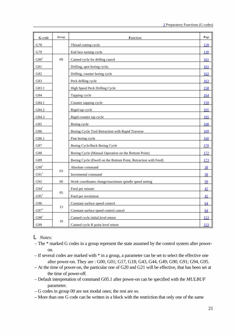
L Notes: – The * marked G codes in a group represent the state assumed by the control system after power-
on. – If several codes are marked with * in a group, a parameter can be set to select the effective one
after power-on. They are : G00, G01; G17, G18; G43, G44, G49; G90, G91; G94, G95. – At the time of power-on, the particular one of G20 and G21 will be effective, that has been set at
the time of power-off. – Default interpretation of command G05.1 after power-on can be specified with the MULBUF
parameter. – G codes in group 00 are not modal ones; the rest are so. – More than one G code can be written in a block with the restriction that only one of the same

3 Preparatory Functions (G codes)
22
function group may used. – Reference to an illegal G code or specification of several G codes belonging to the same group
within a particular block will produce error message 3005 ILLEGAL G CODE.

4 The Interpolation
23
Fig. 4.1-1
4 The Interpolation
4.1 Positioning (G00)
The series of instructionsG00 v
refers to a positioning in the current coordinate system.It moves to the coordinate v. Designation v (vector) refers here (and hereinafter) to all controlledaxes used on the machine-tool. (They may be X, Y, Z, U, V, W, A, B, C) E.g.:
G00 X(U)__ Z(W)__
where X, Z refer to absolute movement, while U, W refer to incremental one (provided U, W arenot selected for axis). The positioning is accomplished along a straight line involving the simultaneous movements of all axesspecified in the block. The coordinates may be absolute or incremental data.The speed of positioning cannot be commanded inthe program because it is accomplished withdifferent values for each axis, set by the builder ofmachine-tool as a parameter. When several axesare being moved at a time, the vectorial resultant ofspeed is computed by the control system in such away that positioning is completed in a minimuminterval of time, and the speed will not exceedanywhere the rapid traverse parameter set for eachaxis.In executing the G00 instruction, the control systemperforms acceleration and declaration in startingand ending the movements, respectively. On completion of the movement, the control will check the"in position" signal when parameter POSCHECK in the field of parameters is 1, or will not do sowhen the parameter is set to 0. It will wait for the "in position" signal for 5 seconds, unless the signalarrives, the control will return the 1020 POSITION ERROR message. The maximum acceptabledeviation from the position can be specified in parameter INPOS.Being a modal code, G00 remains effective until it is re-written by another interpolation command.After power-on, G00 or G01 is effective, depending on the value set in parameter group CODES.
4.2 Linear Interpolation (G01)
The series of instructionsG01 v F
will select a linear interpolation mode. The data written for v may be absolute or incremental values,interpreted in the current coordinate system. The speed of motion (the feed) can be programmed ataddress F.The feed programmed at address F will be accomplished invariably along the programmed path. Itsaxial components:

4 The Interpolation
24
Fig. 4.2-1
Fig. 4.2-2
Feed along the axis X is
Feed along the axis Z is
where x, z are the displacements programmed alongthe respective axes, L is the vectorial length ofprogrammed displacement:
G01 X192 Z120 F0.15
The feed along a rotational axis is interpreted in units ofdegrees per minute (°/min):
G01 C270 F120
In the above block, F120 means 120deg/minute.If the motion of a linear and a rotary axis is combinedthrough linear interpolation, the feed components will bedistributed according to the above formula. E.g. in block
G91 G01 Z100 C45 F120
feed components in Z and B directions are:
Feed along axis Z: mm/min
Feed along axis C: °/min
Being a modal code, G01 is effective until rewritten by another interpolation command. Afterpower-on, G00 or G01 is effective, depending on the parameter value set in group CODES of theparameter field.
4 The Interpolation
25
Fig. 4.3-1
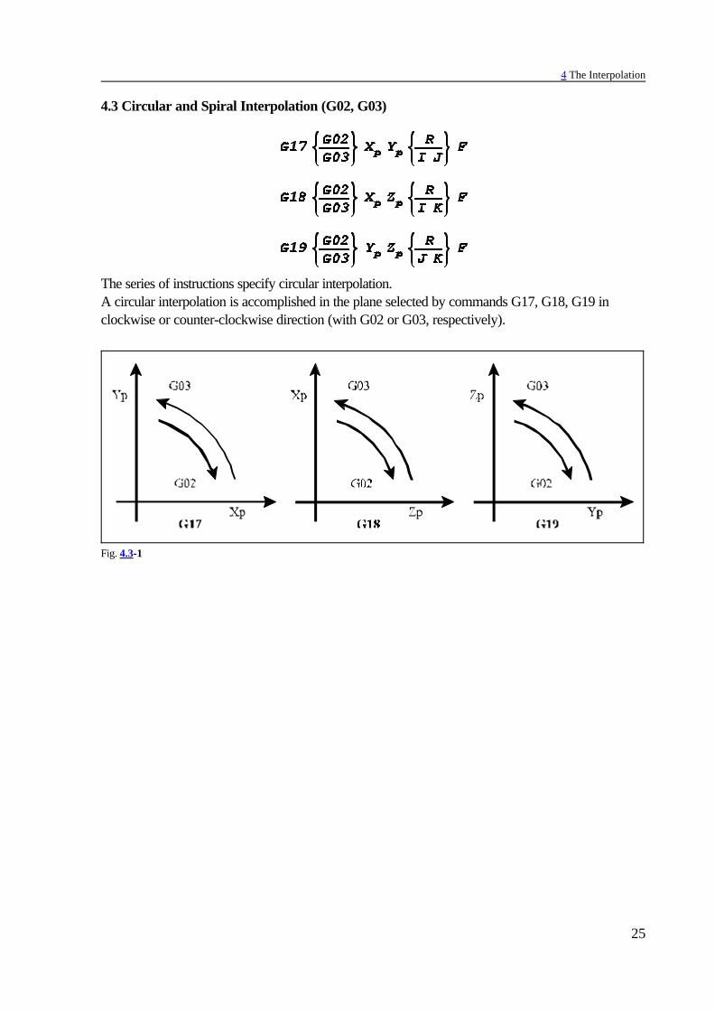
4.3 Circular and Spiral Interpolation (G02, G03)
The series of instructions specify circular interpolation.A circular interpolation is accomplished in the plane selected by commands G17, G18, G19 inclockwise or counter-clockwise direction (with G02 or G03, respectively).

4 The Interpolation
26
Fig. 4.3-2
The above figure shows clockwise (G02) andcounter clockwise (G03) circular directions inplane G18 when the plane is viewed in thepositive-to-negative direction of axis Y. If theplane is viewed in the negative-to-positivedirection of axis Y the interpretation of circulardirections is reversed owing to tool turretarrangements.
Here and hereinafter, the meanings of Xp, Yp, and Zp are:Xp: Axis X or its parallel axis,Yp: Axis Y or its parallel axis,Zp: Axis Z or its parallel axis.
The values of Xp, Yp, and Zp are the end-point coordinates of the circle in the given coordinatesystem, specified as absolute or incremental data.
4 The Interpolation
27
Fig. 4.3-3
Fig. 4.3-4
Fig. 4.3-5
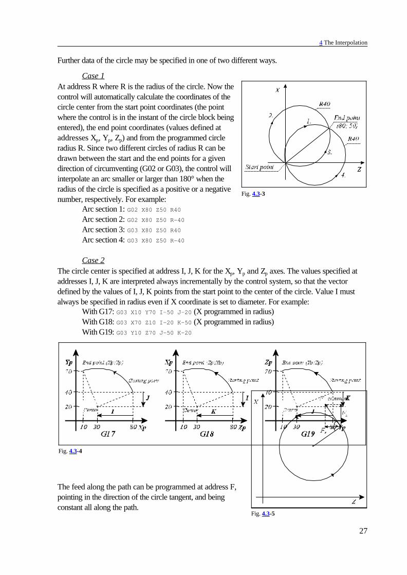
Further data of the circle may be specified in one of two different ways.
Case 1At address R where R is the radius of the circle. Now thecontrol will automatically calculate the coordinates of thecircle center from the start point coordinates (the pointwhere the control is in the instant of the circle block beingentered), the end point coordinates (values defined ataddresses Xp, Yp, Zp) and from the programmed circleradius R. Since two different circles of radius R can bedrawn between the start and the end points for a givendirection of circumventing (G02 or G03), the control willinterpolate an arc smaller or larger than 180° when theradius of the circle is specified as a positive or a negativenumber, respectively. For example:
Arc section 1: G02 X80 Z50 R40Arc section 2: G02 X80 Z50 R-40Arc section 3: G03 X80 Z50 R40Arc section 4: G03 X80 Z50 R-40
Case 2The circle center is specified at address I, J, K for the Xp, Yp and Zp axes. The values specified ataddresses I, J, K are interpreted always incrementally by the control system, so that the vectordefined by the values of I, J, K points from the start point to the center of the circle. Value I mustalways be specified in radius even if X coordinate is set to diameter. For example:
With G17: G03 X10 Y70 I-50 J-20 (X programmed in radius)With G18: G03 X70 Z10 I-20 K-50 (X programmed in radius)With G19: G03 Y10 Z70 J-50 K-20
The feed along the path can be programmed at address F,pointing in the direction of the circle tangent, and beingconstant all along the path.

4 The Interpolation
28
Fig. 4.3-6
Fig. 4.3-7
L Notes: – I0, J0, K0 may be omitted, e.g.
G03 X0 Z100 I-100
– When each of Xp, Yp and Zp is omitted, or the end point coordinate coincides with the start pointcoordinate, then:
a. If the coordinates of the circle center are programmed at addresses, I, J, K the controlwill interpolate a complete circle of 360°. E.g.:
G03 I-100,
b. If radius R is programmed, the control returns error 3012 ERRONEOUS CIRCLE DEF.R.
– When the circle blocka. does not contain radius (R) or I, J, K either,b. or reference is made to address I, J, K outside the selected plane, the control returns
3014 ERRONEOUS CIRCLE DEF. error. E.g. G03 X0 Y100, or (G18) G02 X0Z100 J-100.
– The control returns error message 3011 RADIUS DIFFERENCE whenever the differencebetween the start-point and end-point radii of the circle defined in block G02, G03 exceedsthe value defined in parameter RADDIF.
Whenever the difference of radii issmaller than the value specified inthe above parameter, the controlwill move the tool along a spiralpath in which the radius is varyinglinearly with the central angle.The angular velocity, not the onetangential to the path will beconstant in the interpolation of acircle arc of a varying radius.
The program detail below is an example of how a spiralinterpolation (circle of varying radius) can be specified by theuse of addresses I, K.
G90 G0 X0 Z50G3 Z-20 K-50
4 The Interpolation
29
Fig. 4.3-8
Fig. 4.3-9
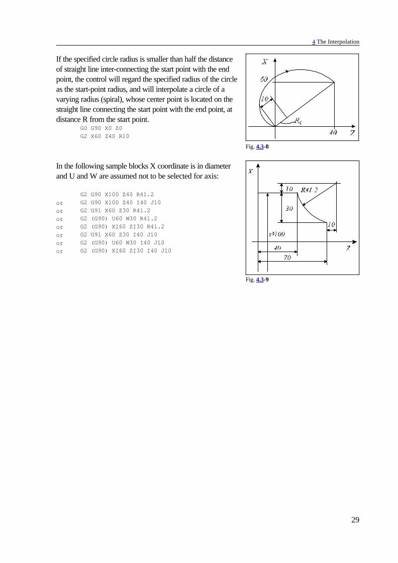
If the specified circle radius is smaller than half the distanceof straight line inter-connecting the start point with the endpoint, the control will regard the specified radius of the circleas the start-point radius, and will interpolate a circle of avarying radius (spiral), whose center point is located on thestraight line connecting the start point with the end point, atdistance R from the start point.
G0 G90 X0 Z0G2 X60 Z40 R10
In the following sample blocks X coordinate is in diameterand U and W are assumed not to be selected for axis:
G2 G90 X100 Z40 R41.2or G2 G90 X100 Z40 I40 J10or G2 G91 X60 Z30 R41.2or G2 (G90) U60 W30 R41.2or G2 (G90) XI60 ZI30 R41.2or G2 G91 X60 Z30 I40 J10or G2 (G90) U60 W30 I40 J10or G2 (G90) XI60 ZI30 I40 J10

4 The Interpolation
30
Fig. 4.4-1
Fig. 4.4-2
4.4 Equal Lead Thread Cutting (G33)
The instructionG33 v F QG33 v E Q
will define a straight or taper thread cutting of equal lead.The coordinates of maximum two axes can bewritten for vector v. The control will cut atapered thread if two coordinated data areassigned to vector v. The control will take thelead into consideration along the long axis.If "<45°, i.e. Z>X, the programmed lead willbe taken into account along axis Z, if ">45°, i.e. X>Z, the control will take theprogrammed lead along axis X.The lead can be defined in one of two 2 ways. – If the lead is specified at address F, the data
will be interpreted in mm/rev orinch/rev. Accordingly, F2.5 has to beprogrammed if a thread of 2.5 mm lead is to be cut.
– If the pitch is specified at address E, the control will cut an inch thread. Address E is interpretedas number of ridges per inch. If, e.g., E3 is programmed, the control will cut a threada"=25.4/3=8.4667mm lead.
The shift angle of the thread start is specified at address Q expressed in degrees from the zero pulseof the spindle encoder. A multiple thread can be cut by an adequate programming of the value of Q,i.e., the control can be programmed here for the particular angular displacements of the spindle, atwhich the various threads are to be cut. If, e.g., a double thread is to be cut, the first and the secondstarts will be commenced from Q0 (no special programming is needed) and from Q180,respectively.G33 is a modal function. If several thread-cutting blocks are programmed in succession,threads can be cut in any arbitrary surfacelimited by straight lines.
The control is synchronized to the zero pulse of the spindle encoder in the first block, nosynchronization will be performed in the subsequent blocks resulting in a continuous thread in eachsection of lines. Hence the programmed shift angle of the thread start (Q) will also be taken intoaccount in the first block.

4 The Interpolation
31
Fig. 4.4-3
Fig. 4.5-1
An example of programming a thread-cutting:
G0 G90 X50 Z40U-30G33 U10 W38 F2G0 U20W-38
In the example above X is specified in diameter.
L Notes: – The control returns error message 3020 DATA
DEFINITION ERROR G33 if more than twocoordinates are specified at a time in the thread-cutting block, or if both addresses F and Eare specified simultaneously.
– Error message 3022 DIVIDE BY 0 IN G33 is produced when 0 is specified for address E in thethread-cutting block.
– An encoder has to be mounted on the spindle for the execution of command G33. – In the course of command G33 being executed, the control will take the feed and spindle override
values automatically to be 100%; the effect of the stop key will only prevail after the blockhas been executed.
– On account of the following error of the servo system, overrun and run out allowances have to beprovided for the tool in addition to the part at the beginning and end of the thread in order toobtain a constant lead all along the part.
– In the course of thread-cutting the feed (in mm/minute) may not exceed the value selected in thegroup of parameters FEEDMAX.
– In the course of thread-cutting the speed (r.p.m) of the spindle may not exceed the maximumspeed permissible for the spindle encoder mechanically and electrically (the maximum outputfrequency).
4.5 Variable-Lead Thread Cutting (G34)
CommandG34 v F Q K
cuts straight or tapered threads of variable-lead. The interpretation of input data v, F, Qcorresponds to those written for function G33.The interpretation of K:
K: Increase or decrease of thread leadper spindle revolution.
The value of K ranges from 0.001 mm/rev (0.0001 inch/rev) to 500 mm/rev (10 inch/rev).

4.6 Polar Coordinate Interpolation (G12.1, G13.1)
32
Fig. 4.6-1
4.6 Polar Coordinate Interpolation (G12.1, G13.1)
Polar coordinate interpolation is a control operation method, in case of which the work described ina Cartesian coordinate system moves its contour path by moving a linear and a rotary axis.Command
G12.1switches polar coordinate interpolation mode on. The path of the milling tool can be described in thesucceeding part program in a Cartesian coordinate system in the usual way by programming linearand circular interpolation, by taking the tool radius compensation into account. The command mustbe issued in a separate block and no other command can be written beside.Command
G13.1switches polar coordinate interpolation mode off. The command must be issued in a separateblock and no other command can be written beside. It always registers state G13.1 after power-on or reset.
Plane selectionA plane determining the address of the linear and the rotary axis to be applied must be selectedbefore switching polar coordinate interpolation on.
CommandG17 X_ C_
selects axis X for linear axis, while as for the rotary axis it is axis C. The virtual axis is indicated withC’ on the diagram, the programming of which is implemented by defining length measures.With the help of commands
G18 Z_ B_G19 Y_ A_
further linear and rotary axes can be selected together in the above mentioned way.
Work zero point offset in the course of polar coordinate interpolationIn case of using polar coordinate interpolation the origin of the applied work coordinate system mustbe chosen so that it coincides with the rotation axis of the circular axis.
Position of the axes when polar coordinate interpolation is switched onBefore switching polar coordinate interpolation on (command G12.1) make sure that the circularaxis position is 0. The linear axis position can either be negative or positive but it cannot be 0.

4.6 Polar Coordinate Interpolation (G12.1, G13.1)
33
Programming length coordinates in the course of polar coordinate interpolationIn the switched-on state of the polar coordinate interpolation length coordinate data may beprogrammed on both axes belonging to the selected plane; The rotary axis in the selected planefunctions as the second (virtual) axis. If e.g. axes X and C have been selected by means ofcommand G17 X_ C_ address C can be programmed like axis Y in the case of plane selection G17X_ Y_.The programming of the first axis being in diameter does not influence the programming of thevirtual axis, the coordinate data must always be given in radius for the virtual axis. If, e.g., polarcoordinate interpolation is executed in plane X C the value written at address C must be specified inradius, independent of address X given in diameter or radius.
Move of axes not taking part in polat coordinate interpolationThe tool on these axes moves normally, independent of the switched-on state of the polarcoordinate interpolation.
Programming circular interpolation in the course of polar coordinate interpolation Definition of a circle in polar coordinate interpolation mode is possible as known by means of theradius or by programming the circle center coordinates. In the latter case addresses I, J, K must beused according to the selected plane as seen below:G17 X_ C_G12.1...G2 (G3) X_ C_ I_ J_
G18 Z_ B_G12.1...G2 (G3) B_ Z_ I_ K_
G19 Y_ A_G12.1...G2 (G3) Y_ A_ J_ K_
Use of tool radius compensation in case of polar coordinate interpolation Commands G41, G42 can be used customary in polar coordinate interpolation. The followingrestrictions must be considered regarding its application: – Switch-on of polar coordinate interpolation (command G12.1) is only possible in state G40, – If G41 or G42 is switched on in state G12.1, G40 must be programmed before switching polar
coordinate interpolation off (command G13.1).
Programming restrictions in the course of polar coordinate interpolationThe below commands cannot be used in the switched-on state of polar coordinate interpolation: – plane change: G17, G18, G19, – coordinate transformations: G52, G92, – work coordinate system change: G54, ..., G59, – orientation in machine coordinate system: G53.
Feed in the course of polar coordinate interpolationInterpretation of feed in polar coordinate interpolation is tangential speed as in case of right angleinterpolation: The relative speed of piece and tool is defined.With polar coordinate interpolation the path described in a Cartesian coordinate system is done bymoving a linear and a rotary axis. As the tool center approaches the circular axis of rotation, therotary axis should have to take larger and larger steps within a time unit so that the path speed isconstant. However the maximum speed permitted for the rotary axis defined by parameter limitscircular axis speed. Therefore, near to the origin the control decreases feed step by step for therotary axis speed not to exceed all limits.

4.6 Polar Coordinate Interpolation (G12.1, G13.1)
34
Fig. 4.6-2
Fig. 4.6-3
The diagram beside shows the cases whenstraight lines parallel to axis X (1, 2, 3, 4) areprogrammed. )x move belongs to theprogrammed feed within a time unit. Differentangular moves (n1, n2, n3, n4) belong to )xmove for each straight lines (1, 2, 3, 4).Apparently, the closer the machining gets to theorigin the larger angular movement the rotaryaxis has to make within a time unit in order tokeep the programmed feed.In case the angular move to be made within atime unit exceeds the value of parameterFEEDMAX set for rotary axis the controlgradually decreases the tangential feed.With these in mind, programs in case of whichthe tool center moves close to the origin are tobe avoided.
ExampleBelow an example forthe use of polarcoordinateinterpolation is shown.The axes taking partin the interpolation:Axes X (linear axis)and C (rotary axis).Axis X isprogrammed indiameter, while that ofaxis C is in radius.
%O7500(POLAR COORDINATE INTERPOLATION)
...N050 T808N060 G59 (start position of coordinate system G59 in
direction X on rotary axis C)N070 G17 G0 X200 C0 (select plane X, C; orientation to coordinate
XÖ0, C=0)

4.6 Polar Coordinate Interpolation (G12.1, G13.1)
35
N080 G94 Z-3 S1000 M3N090 G12.1 (polar coordinate interpolation on)N100 G42 G1 X100 F1000N110 C30N120 G3 X60 C50 I-20 J0N130 G1 X-40N140 X-100 C20N150 C-30N160 G3 X-60 C-50 R20N170 G1 X40N180 X100 C-20N190 C0N200 G40 G0 X150N210 G13.1 (polar coordinate interpolation off)N220 G0 G18 Z100 (Retract tool, select plane X, Z)...
%

4.7 Cylindrical Interpolation (G7.1)
36
Fig. 4.7-1
4.7 Cylindrical Interpolation (G7.1)
Should a cylindrical cam grooving be milled on a cylinder mantle, cylindrical interpolation is to beused. In this case the rotation axis of the cylinder and of a rotary axis must coincide. The rotary axismovements are specified in the program in degrees, which are converted into linear movement alongthe mantle by the control in function of the cylinder radius, so that linear and circular interpolationcan be programmed together with another linear axis. The movements resulted after theinterpolations, are re-converted into movement in degrees for the rotary axis.Command cylindrical interpolation on
G7.1 Qrswitches cylindrical interpolation on, where
Q: address of rotary axis taking part in the cylindrical interpolation,r: cylinder radius.
If for example the rotary axis acting in cylindrical interpolation is axis C and the cylinder radius is 50mm, cylindrical interpolation is switched on by means of command G7.1 C50.In the succeeding part program the path to be milled on the cylinder mantle can be described byspecifying linear and circular interpolation. The coordinate for the linear axis must be given in mm,while that of the rotary axis in degrees (°).Command cylindrical interpolation off
G7.1 Q0switches cylindrical interpolation off, i.e. code G corresponds to that of the switch-on, except for theaddress of rotary axis being 0.The cylindrical interpolation indicated in the above example (G7.1 C50) can be switched off with thehelp of command G7.1 C0.Command G7.1 must be issued in a separate block.
Plane selectionThe plane selection code is always determined by the name of thelinear axis parallel to the rotary axis. The rotary axes parallel toaxes X, Y and Z are axes A, B and C, respectively.G17 X A orG17 B Y
G18 Z C or G18 A X
G19 Y B orG19 C Z
Circular interpolationIt is possible to define circular interpolation in cylindricalinterpolation mode, however only by specifying radius R.No circular interpolation can be executed in case ofcylindrical interpolation by giving the circle center (I, J, K).The circle radius is always interpreted in mm or inch, never indegree.For example circular interpolation between axes Z and C can be specified in two ways:G18 Z_ C_G2 (G3) Z_ C_ R_
G19 C_ Z_G2 (G3) C_ Z_ R_

4.7 Cylindrical Interpolation (G7.1)
37
Fig. 4.7-2
28 651
1800 5. .mm mm⋅
°°
⋅ =π
Application of tool radius compensation in case of cylindrical interpolationCommands G41, G42 can be used in the usual manner in the switched-on state of cylindricalinterpolation. Though the following restrictions are in effect regarding its application: – Switch-on of cylindrical interpolation (command G7.1 Qr) is only possible in state G40. – Should G41 or G42 be switched on in cylindrical interpolation mode, G40 must be programmed
before switching cylindrical interpolation off (command G7.1 Q0).
Programming restrictions in the course of cylindrical interpolationThe following commands are not available in the switched-on state of cylindrical interpolation: – plane selection: G17, G18, G19, – coordinate transformations: G52, G92, – work coordinate system change: G54, ..., G59, – positioning in machine coordinate system: G53, – circular interpolation by giving circle center (I, J, K), – drilling cycles.
ExampleThe diagram beside shows apath milled 3 mm deep onthe mantle of an R=28.65-mm-radial cylinder. Rotatingtool T606 is parallel to theaxis X.. 1° movement on thecylinder mantle is:
The axis order seen on thediagram corresponds toplane selection G19.
%O7602(CYLINDRICAL INTERPOLATION)...N020 G0 X200 Z20 S500 M3 T606N030 G19 Z-20 C0 (G19: select plane C–Z)N040 G1 X51.3 F100N050 G7.1 C28.65 (cylindrical interpolation on, rotary
axis: C, cylinder radius: 28.65mm)N060 G1 G42 Z-10 F250N070 C30N080 G2 Z-40 C90 R30N090 G1 Z-60N100 G3 Z-75 C120 R15N110 G1 C180N120 G3 Z-57.5 C240 R35N130 G1 Z-27.5 C275

4.7 Cylindrical Interpolation (G7.1)
38
N140 G2 Z-10 C335 R35N150 G1 C360N160 G40 Z-20N170 G7.1 C0 (cylindrical interpolation off)N180 G0 X100...%
5 The Coordinate Data
39
Fig. 5.1-1
5 The Coordinate Data
5.1 Absolute and Incremental Programming (G90, G91), Operator I
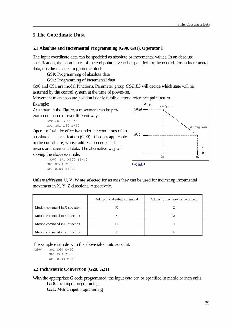
The input coordinate data can be specified as absolute or incremental values. In an absolutespecification, the coordinates of the end point have to be specified for the control, for an incrementaldata, it is the distance to go in the block.
G90: Programming of absolute dataG91: Programming of incremental data
G90 and G91 are modal functions. Parameter group CODES will decide which state will beassumed by the control system at the time of power-on.Movement to an absolute position is only feasible after a reference point return.Example:As shown in the Figure, a movement can be pro-grammed in one of two different ways.
G90 G01 X100 Z20G91 G01 X60 Z–40
Operator I will be effective under the conditions of anabsolute data specification (G90). It is only applicableto the coordinate, whose address precedes it. Itmeans an incremental data. The alternative way ofsolving the above example:
(G90) G01 XI60 ZI–40G01 XI60 Z20G01 X100 ZI–40
Unless addresses U, V, W are selected for an axis they can be used for indicating incrementalmovement in X, Y, Z directions, respectively.
Address of absolute command Address of incremental command
Motion command in X direction X U
Motion command in Z direction Z W
Motion command in C direction C H
Motion command in Y direction Y V
The sample example with the above taken into account:(G90) G01 U60 W-40 G01 U60 Z20 G01 X100 W-40
5.2 Inch/Metric Conversion (G20, G21)
With the appropriate G code programmed, the input data can be specified in metric or inch units.G20: Inch input programmingG21: Metric input programming

5 The Coordinate Data
40
At the beginning of the program, the desired input unit has to be selected by specifying theappropriate code. The selected unit will be effective until a command of opposite meaning is issued,i.e., G20 and G21 are modal codes. Their effect will be preserved even after power-off, i.e., the unitprevailing at the time of power-off will be effective after power-on.The change of the unit will affect the following items:
– Coordinate and compensation data,– Feed,– Constant surface speed– Position, compensation and feed displays.
5.3 Specification and Value Range of Coordinate Data
Coordinate data can be specified in 8 decimal digits.The decimal point will be interpreted as the function of the unit of measure applied: – X2.134 means 2.134 mm or 2.134 inch, – B24.36 means 24.36 degrees when address B refers to a rotary axis.The use of a decimal point is not mandatory. – X325 means e.g. 325 mm.The leading zeros may be omitted. – .032=0.032The trailing zeros may be omitted behind the decimal point. – 0.320=.32The control will interpret a number with more decimals defined by the increment system. Forexample, command X1.23456 will be, when IS-B increment system is selected, interpreted as – 1.235 mm (metric unit), – 1.2346 inch (inch unit).Accordingly, the input data will be output as rounded values.The value ranges of the length coordinates are shown in the Table below.
input unit output unit incrementsystem
value range of lengthcoordinates
unit ofmeasure
mm mm
IS-A ± 0.01-999999.99
mmIS-B ± 0.001-99999.999
IS-C ± 0.0001-9999.9999
inch mm
IS-A ± 0.001-39370.078
inchIS-B ± 0.0001-3937.0078
IS-C ± 0.00001-393.70078
inch inch
IS-A ± 0.001-99999.999
inchIS-B ± 0.0001-9999.9999
IS-C ± 0.00001-999.99999
mm inch
IS-A ± 0.01-999999.99
mmIS-B ± 0.001-99999.999
IS-C ± 0.0001-9999.9999

5 The Coordinate Data
41
Fig. 5.4-1
The value ranges of angular coordinates:
increment system value range of angular coordinates unit of measure
IR-A ± 0.01-999999.99
degreesIR-B ± 0.001-99999.999
IR-C ± 0.0001-9999.9999
5.4 Programming in Radius or Diameter
Since the section of a turned work is generallya circle, sizes in direction of X axis can also bespecified in diameter. The following parameterdetermines if the X-direction size is interpretedby the control in radius or diameter:In case of programming in radius:
4762 DIAM=0In case of programming in diameter:
4762 DIAM=1When programing in diameter the least inputincrement programable is 1. In this case thecontrol steps ½ increments. E.g., ifINCRSYSTB=1 the least command incrementis 0.001 mm and the control steps 0.0005 mmin radius.If the parameter is set to programming diameters, the below cases must be taken into account:
Case Note
Absolute move command in X direction Specified with a diameter value
Incremental move command in X direction Specified with a diameter value (D2 –D1 in the figure)
X component of coordinate system offset Specified with a diameter value
X component of tool length offset Specified with a diameter value
Parameters in canned cycles, such as cutting depthalong X axis
Always specified with a radius value
Radius designation in circular interpolation (R, I) Always specified with a radius value
Display of X axis position Displayed as diameter value
Feedrate along X axis in facing Always specified in radius/rev or radius/min
Increment size in incremental jog and handwheelmode
1 increment=1:m in diameter

5 The Coordinate Data
42
5.5 Rotary Axis Roll-over
This function can be used in case of rotary axes, i.e., if address A, B or C is selected for operatingrotary axis. Handling of roll-over means, that the position on the given axis is not registered betweenplus and minus infinity, but regarding the periodicity of the axis, e.g., between 0/ and 360/.
Selecting rotary axisThe selection can be executed by setting parameter 0182 A.ROTARY, 0185 B.ROTARY or 0188C.ROTARY to 1 for axes A, B or C, respectively. If among these parameters one is set to 1 – the control does not execute inch/metric conversion for the appropriate axis, – roll-over function can be enabled for that axis by setting the appropriate parameter ROLLOVEN
to 1.
Enabling the handling of roll-overThe function is affected by setting parameter 0241 ROLLOVEN_A, 0242 ROLLOVEN_B or0243 ROLLOVEN_C to 1 for axes A, B or C, respectively, provided the appropriate axis is arotary one. If the given parameter ROLLOVEN_x – =0: the rotary axis is regarded as linear axis and the setting of further parameters is uneffective, – =1: handling of roll-over is applied for the rotary axis, the essence of which is discussed below.
Specifying path per roll-overThe path per one roll-over of the axis is defined at parameter 0261 ROLLAMNT_A, 0262ROLLAMNT_B or 0263 ROLLAMNT_C in input increment for axes A, B or C, respectively.Thus if the control is operating in increment system B and the axis rotates 360° per one roll-over,the value to be written at the appropriate parameter is 360000.With the help of the above parameter settings the control always displays the position of the rotaryaxis in range 0°- +359.999° independent of the direction of rotation and the number of revolutions.

5 The Coordinate Data
43
Movement of rotary axis in case of absolute programmingIn case of absolute data input, when handling of roll-over is enabled for rotary axis(ROLLOVEN_x=1), the axis never moves more than that set at appropriate parameterROLLAMNT_x. That is, if, e.g., ROLLAMNT_C=360000 (360/), the maximum movement is359.999°.For the movement direction to always be according to the sign of position given at the axis addressor in the shorter way can be set on the basis of parameter 0244 ABSHORT _A, 0245ABSHORT_B or 0246 ABSHORT_C. If appropriate parameter ABSHORT_x – =0: it always moves in the direction of the sign of the programmed position – =1: it always moves in the shorter direction.
0188 C.ROTARY=1,0243 ROLLOVEN_C=10263 ROLLAMNT_C = =360000
Block programmed by absolutecoordinate input
Movement affectedby block
Position atblock end
0246 ABSHORT_C=0
it always moves in direction ofsign programmed at address C
C=0
G90 C450 90 C=90
G90 C0 (0 is a positive number!) 270 C=0
G90 C–90 –90 C=270
G90 C–360 –270 C=0
0246 ABSHORT_C=1
it always moves in the shorterdirection
C=0
G90 C450 90 C=90
G90 C0 –90 C=0
G90 C–90 –90 C=270
G90 C–360 90 C=0

5 The Coordinate Data
44
Movement of rotary axis in case of incremental programmingIn case of programming incremental data input the direction of movement is always according to theprogrammed sign.The appropriate parameter ROLLAMNT_x to be applied for movement setting can be set atparameter 0247 RELROUND_A, 0248 RELROUND_B or 0249 RELROUND_C for axis A, Bor C, respectively. If the appropriate parameter RELROUND_x – =0: parameter ROLLAMNT_x is out of use, i.e. the movement can be greater than 360/, – =1: parameter ROLLAMNT_x is in use. If, e.g., ROLLAMNT_C=360000 (360/), the largest
movement on axis C may be 359.999°.
0188 C.ROTARY=1,0243 ROLLOVEN_C=10263 ROLLAMNT_C = =360000
Block programmed byincremental data input
Movement affectedby block
Position atblock end
0249 RELROUND_C=0
parameter ROLLAMNT_C is out ofuse
C=0
G91 C450 450 C=90
G91 C0 0 C=90
G91 C–90 –90 C=0
G91 C–360 –360 C=0
0249 RELROUND_C=1
parameter ROLLAMNT_C is in use
C=0
G91 C450 90 C=90
G91 C0 0 C=90
G91 C–90 –90 C=0
G91 C–360 0 C=0

6 The Feed
45
Fig. 6.2-1
6 The Feed
6.1 Feed in Rapid Travers
G00 commands a positioning in rapid traverse.The value of rapid traverse for each axis is set by parameter by the builder of the machine. The rapidtraverse may be different for each axis.When several axes are performing rapid traverse motions simultaneously, the resultant feed will becalculated in such a way that the speed component of each axis will not exceed the particular rapidtraverse value (set as a parameter), and the positioning is accomplished in a minimum of time.Rapid traverse rate is modified by the rapid traverse override switch that can be
F0: Defined by parameter RAPOVER in %,and 25%, 50%, 100%.
The rapid traverse rate will not exceed 100%. Rapid traverse will be stopped if the state of the feedrate override switch is 0%.In lack of a valid reference point, the reduced rapid traverses defined by the machine tool builder byparameter will be effective for each axis until the reference point is returned.Rapid traverse override values can be connected to the feedrate override switch.When the slide is being moved by the jog keys, the speed of rapid traverse is different from therapid traverse in G00, it is also selected by parameters separately for each axis. Appropriately it islower than the speed of positioning for human response times.
6.2 Cutting Feed Rate
The feed is programmed at addressF.The programmed feed isaccomplished in blocks of linear(G01) and circular interpolations(G02, G03).The feed is accomplishedtangentially along the programmedpath.
F - tangential feed (programmed value)Fx - feed component in the X directionFz - feed component in the Z direction
Except for override and stop inhibit states (G63), the programmed feed can be modified over therange of 0 to 120% with the feed-override switch.

6 The Feed
46
The feed value (F) is modal. After power-on, the feed value set at parameter FEED will beeffective.
6.2.1 Feed per Minute (G94) and Feed per Revolution (G95)
The unit of feed can be specified in the program with the G94 and G95 codes:G94: Feed per minuteG95: Feed per revolution
The term "feed/minute" refers to a feed specified in units mm/minute, inch/minute or degree/minute.The term "feed/rev" refers to the feed accomplished in a revolution of the spindle, in units of mm/rev,inch/minute or deg/rev. A G95 cannot be programmed unless the spindle is equipped with anencoder.Modal values. After power-on, state G94 or G95 will be selected with reference to parametergroup CODES. State G94/G95 will be unaffected the rapid traverse, it is invariably in units ofminutes.

6 The Feed
47
The Table below shows the maximum programmable range of values at address F, for variouscases.
inputunits
outputunits
incrementsystem
value range of address F unit
mm mm
IS-A 0.001 - 250000 mmor
deg/minIS-B 0.0001 - 25000
IS-C 0.00001 - 2500
IS-A 0.0001 - 5000 mmor
deg/revIS-B 0.00001 - 500
IS-C 0.000001 - 50
inch mm
IS-A 0.0001 - 9842.5197 inchor
deg/minIS-B 0.00001 - 984.25197
IS-C 0.000001 - 98.25197
IS-A 0.00001 - 196.85039 inchor
deg/revIS-B 0.000001 - 19.685039
IS-C 0.0000001 - 1.9685039
inch inch
IS-A 0.0001 - 25000 inchor
deg/minIS-B 0.00001 - 2500
IS-C 0.000001 - 250
IS-A 0.00001 - 500 inchor
deg/revIS-B 0.000001 - 50
IS-C 0.0000001 - 5
mm inch
IS-A 0.001 - 250000 mmor
deg/minIS-B 0.0001-25000
IS-C 0.00001-2500
IS-A 0.0001 - 5000 mmor
deg/revIS-B 0.00001-500
IS-C 0.000001-50
6.2.2 Clamping the Cutting Feed
The maximum programmable feed on a particular machine can be clamped (set as a parameter) bythe manufacturer of the machine. The value set there invariably refers to minutes. That value is alsothe speed of DRY RUN. If a programmed feed higher than that is set, the control will clamp it

6 The Feed
48
Fig. 6.3-1
Fig. 6.3-2
Fig. 6.3-3
automatically in the course of program execution.The maximum jog feed can also be clamped separately by parameters for human response times.
6.3 Automatic Acceleration/Deceleration
In rapid traverse, the control will automaticallyperform a linear acceleration and lineardeceleration when starting and ending amovement. The extent of acceleration is definedby the machine tool builder, in parameterACCn, depending on the dynamics of themachine.
In feed motions the tangential (programmed)feed value will be assumed by the control inlinear acceleration, inversely, its value will bedecreased by linear deceleration. Thistechnique offers the advantage over traditional(exponential) accelerations that the machine willsooner attain the desired speed (assuming agiven time constant adopted in both cases).Thus the times of acceleration and deceleration(i.e., the times of actual slide movements) will bereduced.
Another advantage of linear acceleration overthe exponential one is the lower profiledistortion (i.e., radius error), compared withexponential acceleration, in a high-speedmachining of a circle.

6 The Feed
49
Fig. 6.3-4
Fig. 6.4-1
The control is monitoring the changes intangential speeds. This is necessary to attain thecommanded speed in a process of continuousacceleration, if necessary, through severalblocks. The acceleration to the new feed (higherthan the previous one) is commenced by thecontrol invariably in the execution of theparticular block, in which the new feed value isspecified. That process may, if necessary, coverseveral blocks. Deceleration to the new feedvalue (lower than the previous one) will bestarted by the control in an appropriate preceding block so that the machining will be started withthe programmed speed in the particular block, in which the new feed value is specified.When moving manually by using jog keys or handwheel, again linear acceleration/deceleration willbe performed. Their values will be defined for each axis by parameters ACC1 through ACC8.
6.4 Feed Control Functions
The override control functions are required when corners are to be machined, and/or when theparticular technology requires the override and stop switches to be canceled.When machining corners, with continuouscutting applied, the slides are - on account oftheir inertia - unable to follow the pathcommanded by the control system. Now thetool will round the corner more or less,depending on the feed.If the workpiece requires sharp corners, thecontrol must be specified to slow down at theend of block, wait until the axes come to a halt, and start the next movement only afterwards.
6.4.1 Exact Stop (G09)
Not being a modal function, G09 will be effective only in the block, in which it has beenprogrammed.At the end of the block, it has been specified, the control will slow down after execution of theinterpolation, and will wait for the "in position" signal. Unless that signal arrives in 5 seconds, thecontrol will return a message 1020 POSITION ERROR.That function can be used for exact machining sharp corners.
6.4.2 Exact Stop Mode (G61)
Modal function, canceled with G62, G63 or G64 command.The control system will slow on completion of each interpolation and wait for the "in position" signal.It will start the next interpolation cycle only afterwards. Unless that signal arrives in 5 seconds, thecontrol will return a message 1020 POSITION ERROR.

6 The Feed
50
Fig. 6.4.5-1
Fig. 6.4.5-2
6.4.3 Continuous Cutting Mode (G64)
Modal function. The control will assume that state after power-on. It will be canceled by codesG61, G62 or G63.In this mode the movement will not come to a halt on the completion of the interpolation, the slideswill not slow down. Instead, the interpolation of the next block will be commenced immediately.Sharp corners cannot be machined in this mode, because they will be rounded off.
6.4.4 Override and Stop Inhibit (Tapping) Mode (G63)
Modal function, canceled by codes G61, G62 or G64.The feed and spindle override and the feed stop is inhibited in this mode. The override values aretaken for 100% (regardless of switch positions). On completion of the interpolation, the system willnot slow down, but start next interpolation cycle immediately.This mode is applicable in various thread cutting and tapping operations.
6.4.5 Automatic Corner Override (G62)
Modal function canceled by any of codes G61, G63 or G64.When inside corners are being machined, higherforces are acting upon the tool before and afterthe corners. To prevent the overload of the tooland developing vibrations, the control will -when G62 commanded - automatically reducethe feed along before and after an inside corner.The corner override is effective under thefollowing conditions. – When tool nose radius compensation is on
(G41, G42). – Between blocks G0, G1, G2, G3. – In movements in the selected plane. – When the corner is machined inside. – When the angle of the corner is smaller then a particular angle defined by parameter. – Over a distance before and after the corner, defined by parameters.The corner override function will be effective between each the following pairs of blocks: Linear-to-linear, linear-to-circular, circular-to-linear, circular-to-circular ones.Inside angle 1 can be selected between 1 and180° by parameter CORNANGLE.

6 The Feed
51
Fig. 6.4.5-3
Fig. 6.4.6-1
Deceleration and acceleration will becommenced at distances Ll and Lg before andafter the corner, respectively. In the case of(circles) arcs, distance Ll and Lg will becalculated by the control along the arc.Distances Ll and Lg will be defined inparameters DECDIST and ACCDIST,respectively.The value of override can be selected as a percent in parameter CORNOVER. The override willbegin to be effective at distance Ll before the corner, and will be effective over distance Lg behindthe corner. The values of feed override and corner override will be taken into account together bythe control:
F* feed override * corner override.Write G09 in the particular block to program an exact stop in state G62.
6.4.6 Internal Circular Cutting Override
With the tool nose radius compensation on (G41, G42), thecontrol will automatically reduce the feed in machining theinside surface of an arc so that the programmed feed will beeffective along the cutting radius. The feed in the center ofthe tool radius is
where Fc is the (corrected) feed of the tool-radius centerR is the programmed radius of circleRc is the corrected radius of circleF is the programmed feed.
The lower limit of automatic feed reduction is set by parameter CIRCOVER, in which the minimumoverride can be specified as a percent. The override for the circle radius is multiplied by the valuesof feed and corner override before it is issued.

7 The Dwell
52
7 The Dwell (G04)
The(G94) G04 P....
command will program the dwell in seconds.The range of P is 0.001 to 99999.999 seconds.
The(G95) G04 P....
command will program the dwell in terms of spindle revolutions.The range of P is 0.001 to 99999.999 revolutions.Depending on parameter SECOND, the delay may refer always to seconds as well, irrespective ofthe states of G94, G95.The dwell implies invariably the programmed delay of the execution of the next block. It is a non-modal function.During dwell in status field 5 indicating interpolation status the message DWL will appear on screento draw the attention of operator why the machine is halted.

8 The Reference Point
53
Fig. 8-1
8 The Reference Point
The reference point is a distinguished positionon the machine-tool, to which the control caneasily return. The location of the reference pointcan be defined as a parameter in the coordinatesystem of the machine. Work coordinate systemcan be measured and absolute positioning canbe done after reference point return. Theparametric overtravel positions and the strokecheck function are only effective after reference-point return.
8.1 Automatic Reference Point Return (G28)
The instruction G28 v
will return the axes defined by vector v to the reference point. The movements consist of two parts. First it will move with linear interpolation in rapid traverse to the intermediate coordinates defined byvector v. The specified coordinates may be absolute or incremental values. The movement isperformed invariably in the current coordinate system .When the end point of linear movement is reached, the tool nose radius compensation vector isdeleted.The coordinates of the intermediate point will be stored for axes defined by vector v.In the second stage it will move from the intermediate point to the reference-point simultaneously ineach axis defined by vector v. The reference-point return is carried out by non-linear movement at aspeed defined for each axis. Afterwards, similar to the manual return, the position will be assumed inthe manner defined by parameters.This is a non-modal code.
L Notes: – Unless there is a valid reference point, incremental values must be assigned to intermediate
coordinates v in command G28. – Programmed in block G28, intermediate coordinates v will be stored until power-off. In other
words, the intermediate value defined in a previous command G28 will continue to be effectfor the coordinates that have not been assigned values in the instantaneous (current)command G28. For example:
G28 X100 intermediate point: X=100, Z=0G28 Z200 intermediate point: X=100, Z=200

8 The Reference Point
54
8.2 Automatic Return to Reference Points 2, 3, 4 (G30)
Series of instructionsG30 v P
will send the axes of coordinates defined at the addresses of vector v to the reference point definedat address P.
P1=reference point 1P2=reference point 2P3=reference point 3P4=reference point 4
The reference points are special positions defined by parameters (REFPOS1, ..., REFPOS4) in thecoordinate system of the machine-tool, used for change positions, e.g., positions of tool change orpalette change. The first reference point is invariably the position of the machine's reference point,i.e., the point to which the control moves when returning to the reference point.The instruction is only applicable after the machine's reference point has been returned.The movement consists of two parts. First it will move by a linear motion to the intermediatecoordinates defined by vector v, with rapid traverse. The specified coordinates may be absolute orincremental values. The movement is carried out invariably in the current coordinate system. Whenthe end point of linear movement is reached, the tool nose radius compensation vector will bedeleted. The coordinates of the intermediate point will be stored in the current coordinate system forthe axes defined by vector v. Stored in this way, the coordinates will overwrite those stored ininstruction G28.In the second phase, the axes defined by vector v will move with rapid traverse from theintermediate point to the reference point selected at address P.The reference point is returned by disregarding the compensation vectors (length, offset, 3dimensional offsets) they need not be deleted before instruction G30 is issued but they will beimplemented by the control when further movements are being programmed. The tool nose radiuscompensation is re-established automatically in the first movement block.A non-modal code.
8.3 Automatic Return from the Reference Point (G29)
Instruction G29 v
will return the control from the reference point along the axes defined in vector v. Following G28and G30, command G29 will be executed in the same manner. The return is accomplished in twostages.In the first stage it will move from the reference point to the intermediate point recorded during theexecution of instruction G28 or G30, in the axes defined by vector v. The coordinates of theintermediate point are modal, in other words, the control will take the previous values into account ifreference is made to an axis, to which no coordinate has been transferred in block G28 or G30preceding G29. It will move to the intermediate point by taking into account the tool length, tooloffset and 3-dimensional tool radius compensations.The coordinates of the intermediary point are effective invariably in the coordinate system of thecurrent workpiece. Accordingly if, e.g., a change of workpiece coordinate system has beenprogrammed after reference point return and before instruction G29, the intermediate point will be

8 The Reference Point
55
Fig. 8.3-1
taken into account in the new coordinate system.In the second phase it will move from the intermediate point to the point v defined in instruction G29.If coordinate v has an incremental value, the displacement will be measured from the intermediatepoint.When the tool nose radius compensation is set up, it will move to the end point by taking intoaccount the compensation vector.A non-modal code.An example of using G30 and G29:
...G90...G30 P1 X200 Z500G29 X150 Z700......

9 Coordinate Systems, Plane Selection
56
Fig. 9-1
Fig. 9.1-1
9 Coordinate Systems, Plane Selection
The position, to which the tool is to be moved, is specified with coordinate data in the program.When 2 axes are available (X, Z), the position of the tool is expressed by two coordinate dataX____ Z____ :The tool position is expressed by as many differentcoordinate data as is the number of axes on themachine. The coordinate data refer invariably to agiven coordinate system.The control will differentiate three different coordinatesystems.
1. the machine coordinate system,2. the workpiece's coordinate system,3. the local coordinate system.
9.1 The Machine Coordinate System
The machine zero point, i.e., the origin of themachine coordinate system, is a point on thegiven machine-tool, that is usually defined by themachine tool builder. The control will define themachine coordinate system at the time ofreturning to the reference point.Once the machine coordinate system has beendefined, it will not be altered by the change ofthe work coordinate system (G54 ... G59) orby other coordinate transformation (G52, G92),only by a power-off of the control system.
9.1.1 Setting the Machine Coordinate System
After a reference point return, the machine coordinate system can be set in parameters. The distanceof the reference point, calculated from the origin of the machine coordinate system, has to be writtenfor the parameter.

9 Coordinate Systems, Plane Selection
57
Fig. 9.2.1-1
9.1.2 Positioning in the Machine Coordinate System (G53)
InstructionG53 v
will move the tool to the position of v coordinate in the machine coordinate system. – Regardless of states G90, G91, coordinates v are always treated as absolute coordinates, – operator I is ineffective when put behind the address of a coordinate, – similar to instruction G00, the movements are performed in rapid traverse, – the positioning is carried out invariably with the selected tool length compensations taken into
account.A G53 instruction can be executed after a reference point return only. G53 is a one-shot commandeffective in the block only, where it has been specified.
9.2 Work Coordinate Systems
The coordinate system applied in cutting the workpiece is referred to as the "work coordinatesystem". Six different coordinate systems can be defined for the workpiece in the control.
9.2.1 Setting the Work Coordinate Systems
In setting mode the locations of the various work coordinate systems can be established in themachine coordinate system, and the necessary offsets can be made.

9 Coordinate Systems, Plane Selection
58
Fig. 9.2.1-2
Fig. 9.2.2-1
Furthermore, all work coordinate system can be offset with a common value. It can also be enteredin setting mode.
9.2.2 Selecting the Work Coordinate System
The various work coordinate system can be selected with instructions G54...G59.G54........work coordinate system 1G55........work coordinate system 2G56........work coordinate system 3G57........work coordinate system 4G58........work coordinate system 5G59........work coordinate system 6
They are modal functions. Their selection before a reference point return is ineffective. After areference point return, work coordinate system 1 (G54) willbe selected.The absolute coordinate data of the interpolation blocks willbe taken into account by the control in the current workcoordinate system.For example, the instruction
G56 G90 G00 X80 Z60
will move the system to point X=80, Z=60 of workcoordinate system 3.

9 Coordinate Systems, Plane Selection
59
Fig. 9.2.2-2
After a change of the work coordinate system,the tool position will be displayed in the newcoordinate system. For instance, there are twoworkpieces on the table. The first workcoordinate system (G54) has been assigned tozero point of one of the workpieces, which hasan offset of X=260, Z=80 (calculated in themachine coordinate system). The second workcoordinate system (G55) has been assigned tothe zero point of the other workpiece, which hasan offset of X=140, Z=180 (calculated in themachine coordinate system). The tool position isX'=140, Z'=90 in X', Z's’ coordinate system(G54). As a result of instruction G55, the tool position will be interpreted in the X", Z" coordinatesystem (X"=260, Z"=–50).
9.2.3 Programmed Setting of the Work Zero Point Offset
It is also programable to set the work coordinate system and the common offset thereof withprogram instructions.This is accomplished with instruction
G10 v L2 Ppwhere
p = 0 sets the common offset,p = 1...6 selecting work coordinate system 1.- 6.v (X, Z, ...) = offset for each axis.
The coordinate data are entered invariably as rectangular (Cartesian) absolute values. G10 is a one-shot (non-modal) instruction.
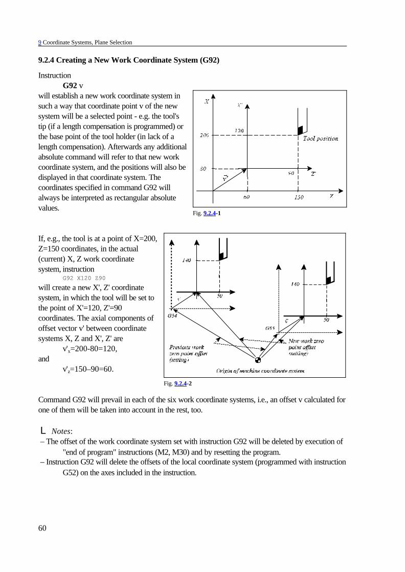
9 Coordinate Systems, Plane Selection
60
Fig. 9.2.4-1
Fig. 9.2.4-2
9.2.4 Creating a New Work Coordinate System (G92)
InstructionG92 v
will establish a new work coordinate system insuch a way that coordinate point v of the newsystem will be a selected point - e.g. the tool'stip (if a length compensation is programmed) orthe base point of the tool holder (in lack of alength compensation). Afterwards any additionalabsolute command will refer to that new workcoordinate system, and the positions will also bedisplayed in that coordinate system. Thecoordinates specified in command G92 willalways be interpreted as rectangular absolutevalues.
If, e.g., the tool is at a point of X=200,Z=150 coordinates, in the actual(current) X, Z work coordinatesystem, instruction
G92 X120 Z90
will create a new X', Z' coordinatesystem, in which the tool will be set tothe point of X'=120, Z'=90coordinates. The axial components ofoffset vector v' between coordinatesystems X, Z and X', Z' are
v'x=200-80=120,and
v'z=150–90=60.
Command G92 will prevail in each of the six work coordinate systems, i.e., an offset v calculated forone of them will be taken into account in the rest, too.
L Notes: – The offset of the work coordinate system set with instruction G92 will be deleted by execution of
"end of program" instructions (M2, M30) and by resetting the program. – Instruction G92 will delete the offsets of the local coordinate system (programmed with instruction
G52) on the axes included in the instruction.

9 Coordinate Systems, Plane Selection
61
Fig. 9.3-1
Fig. 9.3-2
9.3 Local Coordinate System
When writing part programs, it is sometimes more convenient to specify the coordinate data in a"local" coordinate system instead of the work coordinate system.Instruction
G52 vwill create a local coordinate system. – If coordinate v is specified as an absolute value, the origin of the local coordinate system will
coincide with the point v in the work coordinate system. – When specified as an incremental value, the origin of the local coordinate system will be shifted
with v offset (provided a local coordinate system has been defined previously, or else theoffset is produced with respect to the origin of the work coordinate system).
Henceforth any movement command specified in absolute coordinates will be executed in the newcoordinate system. The positions are also displayed in the new coordinate system. The values ofcoordinates v will be treated invariably as Cartesian coordinates.If, e.g., the tool is at point X=200, Z=150coordinates in the current X, Z work coordinatesystem, instruction
G90 G52 X80 Z60
will create a new local X', Z' coordinate system,in which the coordinates of tool will be X'=120,Z'=90. Instruction G52 is used for defining theaxial components of offset vector v' between theX, Z and X', Z' coordinate systems (v'x=80,v'z=60).Now one of two different procedures may beadopted in order to transfer the local coordinatesystem to the point of X", Z" position. – With an absolute data specification: Instruction (G90) G52 X120 Z30 will move the origin of the
X", Z" coordinate system to point X=120, Z=30 in the X, Z work coordinate system. Thecomponents of vector v" will be produced by the specification of v"x=120, v"z=30.
– With an incremental data specification: Instruction G91 G52 X40 Z–30 will move the origin of theX", Z" coordinate system to the point of X'=-40, Z'=30 coordinates in the X', Z' coordinatesystem. The components of vector v will be produced by the specification of vx=40, vz=30.
Indicating the location of the new localcoordinate system in the X, Z work coordinatesystem vector v"=v'+v. Its components:
v"x=80+40=120, v"z=60+(–30)=30.The tool position in the X", Z" coordinatesystem will be X"=80, Z"=120.
InstructionG90 G52 v0
will delete the offset in on coordinates specifiedin v.The local coordinate system will be offset in
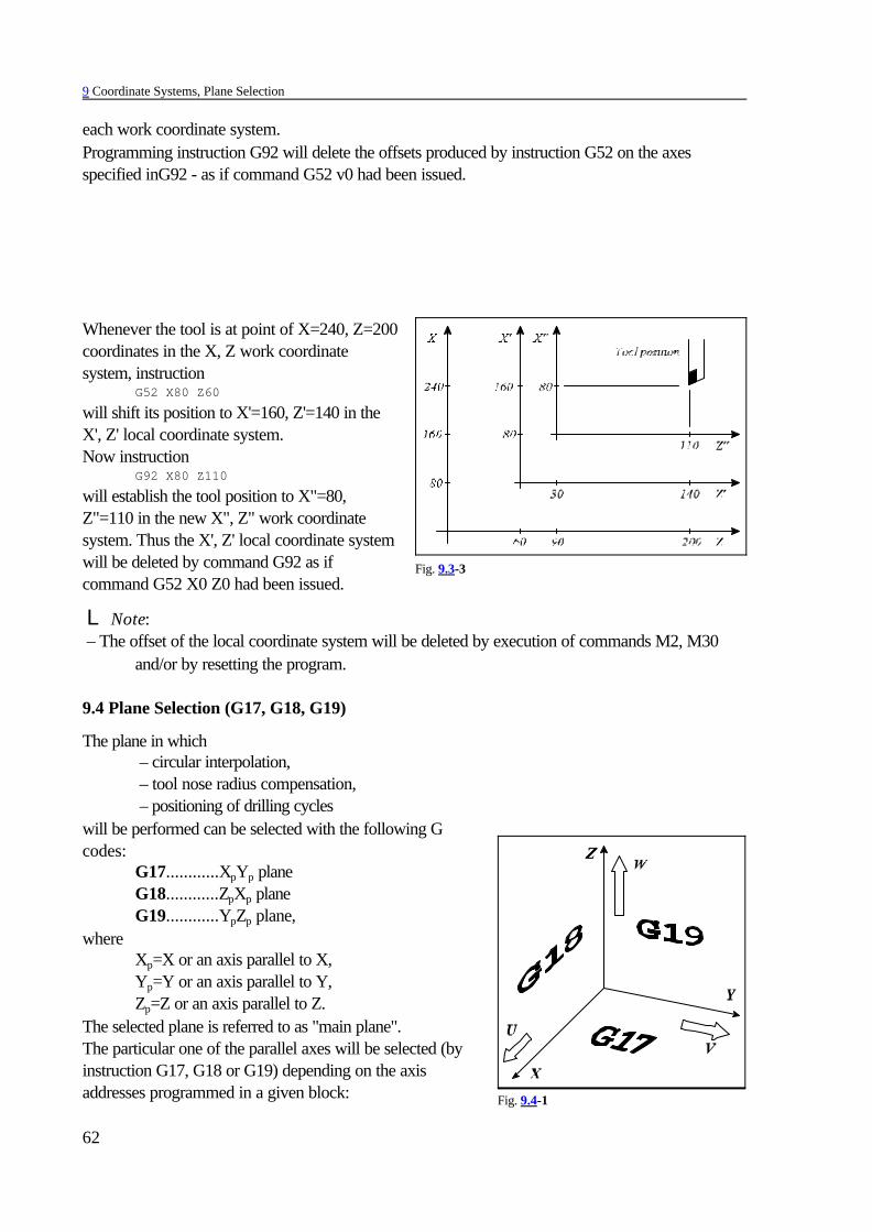
9 Coordinate Systems, Plane Selection
62
Fig. 9.3-3
Fig. 9.4-1
each work coordinate system.Programming instruction G92 will delete the offsets produced by instruction G52 on the axesspecified inG92 - as if command G52 v0 had been issued.
Whenever the tool is at point of X=240, Z=200coordinates in the X, Z work coordinatesystem, instruction
G52 X80 Z60
will shift its position to X'=160, Z'=140 in theX', Z' local coordinate system. Now instruction
G92 X80 Z110
will establish the tool position to X"=80,Z"=110 in the new X", Z" work coordinatesystem. Thus the X', Z' local coordinate systemwill be deleted by command G92 as ifcommand G52 X0 Z0 had been issued.
L Note: – The offset of the local coordinate system will be deleted by execution of commands M2, M30
and/or by resetting the program.
9.4 Plane Selection (G17, G18, G19)
The plane in which – circular interpolation, – tool nose radius compensation, – positioning of drilling cycles
will be performed can be selected with the following Gcodes: G17............XpYp plane
G18............ZpXp planeG19............YpZp plane,
whereXp=X or an axis parallel to X,Yp=Y or an axis parallel to Y,Zp=Z or an axis parallel to Z.
The selected plane is referred to as "main plane".The particular one of the parallel axes will be selected (byinstruction G17, G18 or G19) depending on the axisaddresses programmed in a given block:

9 Coordinate Systems, Plane Selection
63
When X and U, Y and V, Z and W are parallel axes:The XY plane will be selected by G17 X_Y_,the XV plane will be selected by G17 X_V_,the UV plane will be selected by G17 U_V_,the XW plane will be selected by G18 X_W_,the YZ plane will be selected by G19 Y_Z_,the VZ plane will be selected by G19 V_Z_.
Unless G17, G18, G19 is specified in a block, the selected plane remains unchanged:G17 X____ Y____ plane XY
U____ Y____ plane XY remains.Unless there is an axis address specified in the G17, G18, G19 block, the control will consider thebasic axes:
The XY plane will be selected by G17,the XY plane will be selected by G17 X,the UY plane will be selected by G17 U,the XV plane will be selected by G17 V,the ZX plane will be selected by G18,the WX plane will be selected by G18 W.
The selected plane is unaffected by the movement command:(G90) G17 G00 Z100
will select the XY plane, moving the Z axis to the point of coordinate 100.After power-on, the default plane (G17 or G18) is specified according to the parameter groupCODES.The main plane can be selected more times in the same program.Address U, V, W can be selected as a parallel in parameters.

10 The Spindle Function
64
Fig. 10.2-1
10 The Spindle Function
10.1 Spindle Speed Command (code S)
With a number of max. five digits written at address S, the NC will give a code to the PLC.Depending on the design of the given machine-tool, the PLC may interpret address S as a code oras a data of revs/minute.When a movement command and a spindle speed (S) are programmed in a given block, function Swill be issued during or after the motion command. The machine tool builder will define the way ofexecution.The speeds specified at address S are modal values. At the time of power-on, the control willassume value S0. The spindle speed has a minimum and a maximum limit in each gear ratio range.They are defined by the machine-tool builder in parameters and the control does not let the speedoutside of this range.
10.2 Programming of Constant Surface Speed Control
Constant surface speed control function canonly be used in case of infinitely variable speedmain drive. In this case the control can changethe spindle speed so that the tool speed isconstant relative to the surface of theworkpiece and is equal to the programmedvalue.The constant surface speed must be specifiedin function of the input unit on the basis of thetable below:
Input unit Unit of constant surface speed
mm (G21 metric) m/min
inch (G20 inch) feet/min

10 The Spindle Function
65
10.2.1Constant Surface Speed Control Command (G96, G97)
CommandG96 S
switches constant surface speed control function on. The constant surface speed must be specifiedat address S in the unit of measure given in the above table.Command
G97 Scancels constant surface speed control. The desired spindle speed can be specified at address S (inrevs/min). – In order to calculate constant surface speed the coordinate system must be set so that its zero
point coincides with the rotation axis. – Constant surface speed control is effective only after the spindle is started by means of M3 or
M4. – The value is modal even after its calculation has been canceled with the help of command G97.
After power on the default constant surface speed is determined by parameter CTSURFSP. G96 S100 (100 m/min or 100 feet/min)G97 S1500 (1500 revs/min)G96 X260 (100 m/min or 100 feet/min)
– Constant surface speed calculation is also effective in state G94 (feed/min). – If the constant surface speed control is canceled by means of command G97 and a new spindle
speed is not specified the last spindle speed gained in state G96 remains in effect.G96 S100 (100m/min or 100 feet/min)
.
.
.G97 (Revolution belonging to resulting diameter X)
– In case of rapid traverse positioning (block G00) the constant surface speed is not calculatedcontinuously but the revolution belonging to the end-position will be calculated. This isneeded for the spindle speed to avoid unnecessary changes.
– In order to calculate constant surface speed the zero point of the axis, on the basis the spindlespeed is changed, must be set to the spindle rotation axis.
10.2.2 Constant Surface Speed Clamp (G92)
With the help of commandG92 S
the highest spindle speed enabled in case of constant surface speed control can be set. Duringconstant surface speed calculation the control clamps spindle speed to this value. In this case the unitof S is rpm. – After power on as well as if value S has not been clamped by means of command G92 the top
limit of spindle speed in case of constant surface speed control is the maximum valueenabled for the given gear range.
– The maximum revolution value is modal until a new one is programmed or until the control isturned off.

10 The Spindle Function
66
10.2.3 Selecting an Axis for Constant Surface Speed Control
The axis, which position the constant surface speed is calculated from, is selected by parameter1182 AXIS. The logic axis number must be written at the parameter.If other than the selected axis is to be used, the axis from which the constant surface speed is to becalculated can be specified by means of command
G96 P. Interpretation of address P:
P1: X, P2: Y, P3: Z,P4: U, P5: V, P6: W,P7: A, P8: B, P9: C
– The value set at address P is modal. After power on the control activates constant surface speedcontrol to the axis set at parameter AXIS.
10.3 Spindle Position Feedback
In normal machining the NC will issue a speed command to the power amplifier of the spindle,proportional to the programmed speed (value specified at address S). Now this amplifier will beworking in speed-control mode.Some technological tasks may, however, require the spindle to be brought to a particular angularposition. This is referred to as spindle positioning or indexing.Prior to positioning, the NC will set the power amplifier of the spindle to position-controlled mode.In practice this means that the NC will not issue a speed command proportional to code S anymore, instead, it will measure the position of the spindle by the use of an encoder mounted on thespindle, and will issue a command to the servo amplifier in accordance with the desired angulardisplacement (similar to the rest of controlled axes). This is the position feedback.To be able to position the spindle on a particular machine, an encoder has to be mounted on thespindle and the power amplifier of the spindle must be capable of operation in position feedbackmode as well.
10.4 Oriented Spindle Stop
The "spindle orientation" or the "oriented spindle stop" refers to the function of stopping the spindlein a particular angular position. This may be necessary, e.g., for an automatic tool change or for theexecution of some drilling cycles. The possibility of orientation on a particular machine must bespecified by parameter ORIENT1 in parameters. The command of spindle orientation is issued byfunction M19, but it may also be produced by some other function depending on the particularmachine-tool. The orientation may be carried out in one of two different ways.If the spindle cannot be used in position control mode, the orientation is feasible by turning thespindle to a proximity switch mounted on the machine.If the spindle can be used in position control mode, command M19 will cause the control to returnto the zero pulse of the spindle encoder. The control will automatically close the position controlloop.

10 The Spindle Function
67
10.5 Spindle Positioning (Indexing)
A spindle positioning is only feasible after the spindle position control loop has been closed afterorientation. Accordingly, this function is used for closing the loop. The loop will be opened byrotation command M3 or M4.If the value of parameter INDEX1=1 (indicating that the main drive position control loop can beclosed) and the value of parameter INDEX_C1=0, the spindle indexing will be performed byfunction M.Under such conditions function M from the threshold value set on parameter M_NUMB1 toM_NUMB1+360 will be interpreted as a spindle indexing commands, i.e., the threshold number willbe subtracted from the programmed value of M, and the number obtained will be treated as anincremental displacement specified in degrees.Thus, if M_NUMB1=100, command M160 means that the spindle must be turned by 160-100=60degrees from its current position. The direction of rotation is selected by parameter CDIRS1, its rateis selected by parameter RAPIDS1.
10.6 Spindle Speed Fluctuation Detection (G25, G26)
CommandG26
enables spindle speed fluctuation detection, while commandG25
cancels it. After power-on or RESET the control is set to state G26, i.e., spindle speed fluctuationdetection is on. This function signals abnormalities occurring in the course of spindle rotation, as theresult of which, e.g., spindle seizure can be avoided. The speed fluctuation detection is influenced by 4 parameters. These parameters can be overwrittenfrom a program with addresses following command G26. The overwritten parameters are kept uponpower-off. The parameters are overwritten as the effect of command
G26 Pp Qq Rr Dd.The below table contains the parameter interpretations:
name parameter meaning unit value limit
p 5001 TIME time from the issue of a new spindlespeed command to the start ofchecking
100 msec 65535
q 5002 SCERR tolerance of the specified spindlespeed
% 1-50
r 5003 FLUCT% allowable amount of spindle speedfluctuation in the percentage ofprogrammed speed
% 1-50
d 5004 FLUCTW spindle speed fluctuation in absolutevalue
revs/min 65535
The process of speed fluctuation detection is as follows.

10 The Spindle Function
68
Fig. 10.6-2
Fig. 10.6-1
Start of Spindle Speed Fluctuation DetectionAs the effect of new rotation speed the detection is suspended by the control. The speed fluctuationdetection starts when
- the current spindle speedreaches the specified spindlespeed within the tolerance limitdetermined by value "q", or
- the current spindle speed hasnot reached the specified spindlespeed within the tolerance limitdetermined by value "q", but timedetermined by value "p" haselapsed from the command .

10 The Spindle Function
69
Fig. 10.6-3
Detecting ErrorIn the course of detection the control sends error message in case the deviation between current andspecified spindle speed exceeds
- the tolerance limit specified by value "r" inpercent of the command value and- also the absolute tolerance limit specified byvalue "d" When the current speed has exceeded bothtolerance limits, the NC sets flag I656 to PLC. The speed range, in which the NC issuesalarm, can be seen on the 3rd figure. If thespecified spindle speed is under value "S"apparent in the figure, the NC issues alarm,provided the current speed is 0 revs/min formore than 1 second. – The spindle speed fluctuation detection is
effective only if the spindle is mountedwith encoder.
– The specified spindle speed, according towhich the current spindle speed isdetected is calculated by taking theoverride, the revolution range limits and the programmed maximum revolution (G92 S_) inconstant surface speed calculation (G96) into account.
– The spindle speed fluctuation detection is effective only in case of G26 and rotating spindle (stateM3 or M4).
– Command G26 must be programmed in single block.

11 Tool Function
70
11 Tool Function
The first two digits of the number written at address T form the tool number, while the second twodigits form the offset number.Interpretation of the code written at address T:
Meaning of command T1236: Activate tool No. 12 and use offset number 36. – Leading zeroes may be omitted when programming address T: T101=T0101 – If 0 is programmed for tool or only 1 or 2 digits are written at address T tool is not changed, only
a new offset group is called. Meaning of T12: Use offset number 12.When a move command and a tool number (T) are programmed in a given block, T function will beissued during or after execution of the move command. The execution method is determined by thebuilder of the machine.
T n n m m
offset number
tool number

12 Miscellaneous and Auxiliary Functions
71
12 Miscellaneous and Auxiliary Functions
12.1 Miscellaneous Functions (Codes M)
With a numerical value of max. 3 digits specified behind address M, the NC will transfer the code tothe PLC.When a movement command and a miscellaneous function (M) are programmed in a given block,function M will be issued during or after the motion command. The machine tool builder will definethe way of execution.Codes M’s include standard functions, that can be used for special selected functions only. They: M00, M01, M02, M30, M96, M97, M98, M99: Program control codes
M03, M04, M05, M19: Spindle rotation codes M07, M08, M09: Coolant management codes M11, ..., M18: Spindle-range changes codesThe rest of M values can be used without restrictions.When indexing is triggered by M, the M codes of spindle indexing are selected on the basis of aparameter.The control system enables several M codes of different groups to be written in a given block. Inthis case, however, codes M’s have a fixed sequence of execution. The groups and the sequence ofexecution:
group 1 M11, ..., M18 (spindle gear range change)group 2 M03, M04, M05, M19 (spindle management)group 3 M07, M08, M09 (coolant management)group 4 Mnnn (any other function M)group 5 codes M of spindle indexinggroup 6 M00, M01, M02, M30, M96, M97, M98, M99 (program control codes)
The number of M functions that can be programmed in a given block is 5. Only one M of eachgroup can be programmed in a block. Conflicting programming will produce error message 3032CONFLICTING M CODES.The exact functioning of each M code is defined by the builder of the particular machine-tool tomeet its specific requirements. The only exceptions are the program control codes.
The program control M codes are:M00= programmed stop
The stop condition will be generated at the end of the block, in which M00 has been specified. Allmodal functions remain unchanged. It can be restarted by START.
M01= conditional stopIts effect is identical with that of code M00. It will be executed when the CONDITIONAL STOPkey is activated. Unless the appropriate key is set up, it is ineffective.
M02, M30= end of programIt means the end of the main program. All operations are stopped, and the control is "reset". Themachine will be reset by the PLC program. Unless the parameter PRTCNTM differ from it, each ofexecuted M02 or M03 command increase the counters of workpiece.
M98= call of a subprogram (subroutine)It will call a subprogram (subroutine).

12 Miscellaneous and Auxiliary Functions
72
M99= end of subprogram (subroutine)It will cause the execution to return to the position of call.
12.2 Auxiliary Function (Codes A, B, C)
Max. three digits can be specified at each of addresses A, B, C provided one (or all) of thoseaddresses is (are) selected as auxiliary function(s) in parameters. The value specified for the auxiliaryfunction will be transferred to the PLC.When a movement command and an auxiliary function are programmed in a given block, function A,B, C will be issued during or after the motion command. The machine tool builder will define theway of execution.For example, an indexing table can be indexed at address B.
12.3 Sequence of Execution of Various Functions
The various functions written in a given block will be executed by the control in the followingsequence:
1. Tool call: T 2. Spindle range selection: M11, ..., M183. Spindle speed: S4. Spindle management: M03, M04, M05, M195. Coolant: M07, M08, M096. Other function M: Mnnn7. Spindle indexing: With function M8. Function A: A9. Function B: B10. Function C: C11. Program control codes: M00, M01, M02, M30, M96, M97, M98, M99
If the above sequence of executions is not desirable, the block has to be broken up into severalones, with the functions written in the desired sequence in each block.

13 Part Program Configuration
73
13 Part Program Configuration
The structure of the part program has been described already in the introduction presenting thecodes and formats of the programs in the memory. This Section will discuss the procedures oforganizing the part programs.
13.1 Sequence Number (Address N)
The blocks of the program can be specified with serial or sequence numbers. The numbering can beaccomplished at address N. The blocks can be numbered with max. 5 digits at address N. The useof address N is not mandatory. Some blocks can be numbered, others not. The block numbers neednot follow each other in a consecutive order.
13.2 Conditional Block Skip
A conditional block skip can be programmed at the slash address /. The value of the slash addressmay be 1 to 9. Digit 1 to 9 represents serial number of switches .Switch CONDITIONAL BLOCK No. 1 can be found on the operator’s panel of control.The other switches may be provided optionally, their signals can be entered through the interface ofthe control system.If a conditional block skip /n is programmed at the beginning of a block, – that block will be omitted from the execution when the nth switch is on, – that block will be executed when the nth switch is off.
13.3 Main Program and Sub-program
Two different programs are differentiated - main program and subprogram. Repetitive activities maybe involved in machining a component part, that can be described with a particular program detail.In order to avoid writing the repetitive program detail over and over again in the program, they canbe organized into a subprogram to be called from the part program. The structures of the mainprogram and the subprogram have been described in the Introduction.The difference between them is that, whereas the machining is completed after execution of the mainprogram the control is awaiting another START, while after execution of the subprogram it willreturn to the calling program, resuming the machining process at that point.In terms of programming technique, the difference between the two programs lies in the way ofterminating the program. The end of the main program is specified with codes M02 or M30 (notmandatory ones), whereas the sub-program must be terminated with code M99.
13.3.1 Calling the Sub-program
The series of instructionsM98 P....
will generate a subprogram call. As a result, the execution of the program will be resumed at thesubprogram, the number of which is defined at address P. The limit of address P are 1 to 9999.After the execution of the sub-program machining will be continued in the main program with theblock following the subprogram call.

13 Part Program Configuration
74
main program
O0010............
subprogram comment
execution of (main-)program O0010
M98 P0011 –––> O0011 calling sub-programO0011
......
......
......
execution of sub-program O0011
next block <––– M99 return to the callingprogram
......
......resumption of programO0010
The series of instructionsM98 P.... L....
will call the subprogram (specified at address P) repeteatedly in succession specified at address L.The limit of address L is 1 to 9999. Unless L is assigned a value, the sub-program will be calledonce, i.e., the control will assume L=1.Instruction M98 P11 L6 means that subprogram 011 has to be called six times repeatedly.It is also possible to call a subprogram from another subprogram. The subprogram calls can be"nested" to max. 4 levels.
L Notes: – An error message 3069 LEVEL EXCESS is returned when the number of subprogram calls
"nested" exceeds 4. – An error message 3071 MISSING OR FAULTY P is returned when the value of address P
exceeds 9999 or is not specified. – An error message 3072 DEFINITION ERROR L is returned when the value of L is incorrect. – An error message 3073 NOT EXISTING PROGRAM is returned when a program specified with
an identifier at address P is not available in the memory.
13.3.2 Return from a Sub-program
The use of instructionM99
in a sub-program means the end of that sub-program, and the program execution returns to theblock following the call in the calling program.
main program subprogram subprogram subprogram subprogramO0001 >O0011 >O0012 >O0013 >O0014.... .... .... .... ........ .... .... .... ....M98P11 M98P12 M98P13 M98P14 ........< ....< ....< ....< ........ .... .... .... ....M02 M99 M99 M99 M99

13 Part Program Configuration
75
main program
O0010..................
subprogram comment
execution of programO0010
N101 M98 P0011 –––> O0011 calling sub-programO0011
......
......
......
execution of sub-program O0011
N102 ...... <––– M99 return to the nextblock of the callingprogram
......
......resumption of programO0010
The use of instructionM99 P...
in a sub-program means the end of that sub-program, and the program execution returns to theblock of calling program specified at address P. In this case the limit values of P are to 99999.
main program
O0010..................
subprogram comment
execution of programO0010
N101 M98 P0011 –––> O0011 calling sub-programO0011
......
......
......
execution ofsubprogram O0011
N250 ...... <––– M99 P250 return to the N250block of the callingprogram resumption ofO0010
......
......
InstructionM99 (P.....) L....
will rewrite the cycle counter of the calling program. With 0 written for L, the sub-program will becalled only once. If, e.g., subprogram O0011 is called with instruction M98 P11 L20, and a returnis made with instruction M99 L5, subprogram O0011 will be called 6 times. (The limit values of Lare 1 to 9999.)
L Note: – An error message 3070 NOT EXISTING BLOCK NO. P is displayed when the return block
number (P) is not found in the calling program.

13 Part Program Configuration
76
13.3.3 Jump within the Main Program
The use of instructionM99
in the main program will produce an unconditional jump to the first block of the main program, andthe execution of the program will be resumed there. The use of this instruction results in an endlesscycle:
The use of instructionM99 P.....
will produce an unconditional jump to the block specified at address P of the main program, and theexecution of the program will be resumed there. The use of this instruction may result in an endlesscycle:
The possibility of endless cycles can be avoided by specifying the block containing instruction M99in the form /1 M99. Now the jump will be omitted or not, depending on the setting of the conditionalblock skip switch.
O0123N1... <.............M99
O0011 O0011.... ........ M99 P225N128....< ........ ........ N225 <M99 P128 ....

14 The Tool Compensation
77
14 The Tool Compensation
In order not to take the overhang values, tool radii ect. belonging to the different tools into account,the tool characteristics are gathered in a table, namely in the offset table. In case a tool is called inthe part program, the place in the offset table the data of the given tool can be found must be given.Henceforth the control leads the tool in the programmed path by acknowledging the offsets referredto.
14.1 Reference to Tool Offset
Reference to tool offset can be made by the second two digits of the number written at address T.Interpretation of the code written at address T:
Meaning of command T1236: Activate tool No. 12 and call group No. 36 of the offset table ) the leading zeroes may be left when programming address T: T101=T0101 ) If 0 is programmed for the tool number or only one or two digits are written at address T, no tool
replacement occurs, but a new offset group is used. The meaning of T12: Use offset group12.
By the use of the offset number a group of the tool offset table is selected for the control. Theelements of this table are as follows:
Groupnumber
X Y Z R Q
geom. wear geom. wear geom. wear geom. wear
1 123.500 -0.234 87.450 -0.129 267.400 -0.036 1 -0.010 3
2
3
...
47
The tool offset table contains the components of the tool vector in X and Z directions (optionallyalso in Y direction), the tool nose radius (R) as well as the tool state code (Q).
L WarningOffset group 00 is not in the table, its offset values are always zeroes, thus offsetgroup 00 deletes the offset vector.
T n n m m
offset number
tool number

14 The Tool Compensation
78
Fig. 14.1-1
Fig. 14.1 -2
Offsets in X, (Y), Z directions and radiuscompensations (R) can be two types:Geometry and wear offsets.
Geometry value : Length/radius of themeasured tool, signed number.
Wear value : Amount of wear occurringin the course of machining, signednumber.
If an offset group is referred to inprogram at address T the control alwaystakes the sum of geometry and wearvalues as offset amount into account.
For example if reference to Tnn01 is made in theprogram the offset value for X axis on the basis of theabove table according to line 01:123.500+()0.234)=123.266
The same goes for offset values in Z direction (and Y)and also for tool radius offset values (R).

14 The Tool Compensation
79
Fig. 14.1-3
Value limits of geometric and wear offset values:
input unitsystem
output unitsystem
incrementsystem
geometry value wear valuedi-
mension
mm mm
IR-A ±0.01 ÷99999.99 ±0.01÷163.80
mmIR-B ±0.001÷9999.999 ±0.001÷16.380
IR-C ±0.0001÷999.9999 ±0.0001÷1.6380
inch mm
IR-A ±0.001÷9999.999 ±0.001÷6.448
inchIR-B ±0.0001÷999.9999 ±0.0001÷0.6448
IR-C ±0.00001÷99.99999 ±0.00001÷0.06448
inch inch
IR-A ±0.001÷9999.999 ±0.001÷16.380
inchIR-B ±0.0001÷999.9999 ±0.0001÷1.6380
IR-C ±0.00001÷99.99999 ±0.00001÷0.16380
mm inch
IR-A ±0.01÷99999.99 ±0.01÷416.05
mmIR-B ±0.001÷9999.999 ±0.001÷41.605
IR-C ±0.0001÷999.9999 ±0.0001÷4.1605
The direction of imaginary tool nose viewedfrom tool nose center must be also given in theoffset table. Length compensations X and Z aremeasured to the imaginary tool nose.
The imaginary tool nose number (Q) is a one-digit number, its value may be 0,1,...9.
The imaginary tool nose number depends onthe state of the applied coordinate system. Thebelow two figures show the imaginary tool nosenumbers (Q) to be used.

14 The Tool Compensation
80
Fig. 14.1-4 Fig. 14.1-5
The compensation code called is modal, thus the control takes the same offset amounts into accountuntil an other T command is received, i.e. when the compensation values are read by means of a Tcommand, in this case the modification of the offset table (for example by programming G10) doesno longer have an effect on the value read.The offset values of the tool compensation memory are backed up upon power-off.The tool offset memory can also be saved as a part program in the memory.The tool offset values can be set, as well as modified from control panel by means of data input andfrom program by the use of setting command G10. If the current offset value is modified with thehelp of command G10 the current offset register must be re-referred to, because the modified valueis taken into account only in this case.
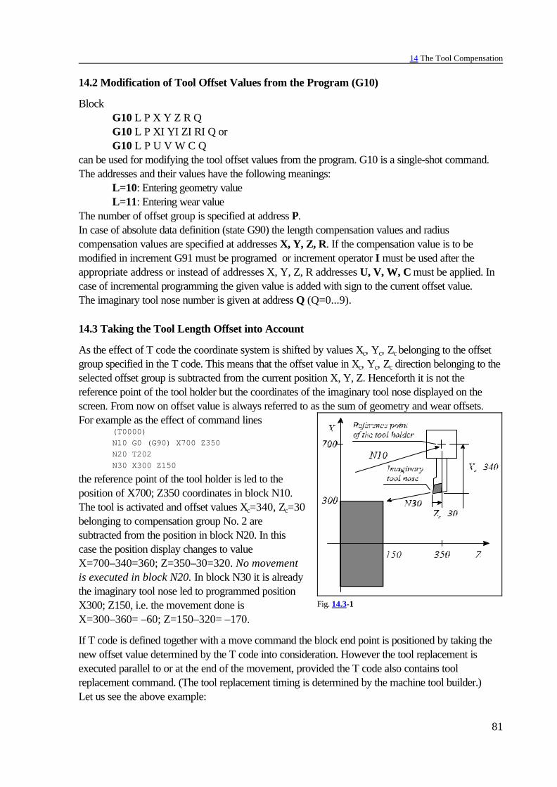
14 The Tool Compensation
81
Fig. 14.3-1
14.2 Modification of Tool Offset Values from the Program (G10)
BlockG10 L P X Y Z R QG10 L P XI YI ZI RI Q orG10 L P U V W C Q
can be used for modifying the tool offset values from the program. G10 is a single-shot command.The addresses and their values have the following meanings:
L=10: Entering geometry valueL=11: Entering wear value
The number of offset group is specified at address P.In case of absolute data definition (state G90) the length compensation values and radiuscompensation values are specified at addresses X, Y, Z, R. If the compensation value is to bemodified in increment G91 must be programed or increment operator I must be used after theappropriate address or instead of addresses X, Y, Z, R addresses U, V, W, C must be applied. Incase of incremental programming the given value is added with sign to the current offset value.The imaginary tool nose number is given at address Q (Q=0...9).
14.3 Taking the Tool Length Offset into Account
As the effect of T code the coordinate system is shifted by values Xc, Yc, Zc belonging to the offsetgroup specified in the T code. This means that the offset value in Xc, Yc, Zc direction belonging to theselected offset group is subtracted from the current position X, Y, Z. Henceforth it is not thereference point of the tool holder but the coordinates of the imaginary tool nose displayed on thescreen. From now on offset value is always referred to as the sum of geometry and wear offsets.For example as the effect of command lines
(T0000)N10 G0 (G90) X700 Z350N20 T202N30 X300 Z150
the reference point of the tool holder is led to theposition of X700; Z350 coordinates in block N10.The tool is activated and offset values Xc=340, Zc=30belonging to compensation group No. 2 aresubtracted from the position in block N20. In thiscase the position display changes to valueX=700–340=360; Z=350–30=320. No movementis executed in block N20. In block N30 it is alreadythe imaginary tool nose led to programmed positionX300; Z150, i.e. the movement done isX=300–360= –60; Z=150–320= –170.
If T code is defined together with a move command the block end point is positioned by taking thenew offset value determined by the T code into consideration. However the tool replacement isexecuted parallel to or at the end of the movement, provided the T code also contains toolreplacement command. (The tool replacement timing is determined by the machine tool builder.)Let us see the above example:

14 The Tool Compensation
82
Fig. 14.3-2
(T0000)N10 G0 (G90) X700 Z350N20 X300 Z150 T202
In this case block N30 is left and the commands of blocks N20 and N30 are pooled. In block N20in the course of movement it is already the imaginary tool nose led to the position of X=300, Z=150coordinates as in the case of block N30 in the previous example. However tool replacement occurseither during or at the end of movement. The latter case may however easily lead to collision, if, e.g.,the overhang of the previous tool is longer than that of the new one and tool replacement is executedby the machine at the end of block. For the above reason it is only expedient to program T codetogether with movement for calling new offset:
N10 G0 (G90) X700 Z350N20 X300 Z150 T02
In the above example no tool replacement is implemented, only offset group No. 2 is called in blockN20.
L Warning!As a consequence of the above, in case the T code results in tool replacement, e.g.turret rotation it is expedient to program the T code in a single block. If the Tcommand executes only offset group change, T code may safely be programmed alsoin move command.
Canceling of tool length compensation
Offset group No. 0 has a special role, it implements compensation canceling. As the effect of command
Tnn00 orT0
the length compensation is canceled (nn: optional tool). The process is the reverse of that ofcompensation call. This means that offset values Xc, Yc, Zc valid previously are added to X, Y, Zimaginary tool nose coordinates and hereafter the reference point coordinates of tool holder are seenin the display. If compensation canceling occurs together with move command the reference point oftool holder is sent to the programmed block end position.For example in sample example
N10 X180 Z120 T202N20 X200 Z180N30 X280 Z210 T200
the movement is compensated by the offsetgroup called as compared to the programmedone in block N10, while the offset, i.e. the oneset in block N10 is canceled in block N30.

14 The Tool Compensation
83
Fig. 14.4-1
Fig. 14.4-2
14.4 Tool Nose Radius Compensation (G38, G39, G40, G41, G42)
If only tool length compensation is used, it is notpossible to turn an accurate tapered line or acircular arc. In this case the imaginary tool noseis guided by the control along the programedpath. Because each tool’s nose has a rounding,the part will be accurate where the path isparallel to one of the axes X or Z. Processingtapered lines or arcs insufficient depth of cut isturned, as it can be seen on the figure beside.
To be able to turn the contour of a workpiece and to specify the points of that formation as per thedrawing in the program (regardless of the radius of the tool nose employed), the control must guidethe tool nose center parallel to the programmed contour, spaced by the tool nose radius from thelatter. The control will determine the distance between the path of the tool nose center and theprogrammed contour in accordance with the compensation value of the tool nose radius referred toby the compensation number of address T.Before turning on the tool noseradius compensation the imaginarytool nose position is registered bythe control. The imaginary toolnose number given at address Q incompensation table is needed tospecify the direction of tool nosecircle center from the imaginarynose. The tool radius (R) is addedto or subtracted from theimaginary tool nose position in Xand Z directions on the basis ofimaginary tool nose number(position A in the figure).Afterwards the tool nose circlecenter is led to the end point of the compensation vector whose length is R and positionedperpendicular to the start point of the programed path (position B in the figure) Next the tool nosecircle center is led parallel to the programmed path of a distance of R from it.The compensation vector is a two-dimensional vector computed over and over again by the controlin each block, modifying the programmed displacements with the compensation vectors effective atthe beginning and end of each block. The length and direction of each compensation vector obtained

14 The Tool Compensation
84
Fig. 14.4-3 Fig. 14.4-4
vary with the compensation value (called at address T) and the geometry of the transition betweenthe two blocks.The compensation vectors are computed in the plane selected by instructions G17, G18, G19. Thisis the plane of tool nose radius compensation. Movements outside of this plane are not influenced bycompensation. If, e.g., plane X, Z is selected in state G18, the compensation vectors will becomputed in that plane. In this case any movement in Y direction it will be unaffected by thecompensation.The compensation plane may not be changed while a tool radius compensation is being computed.Any attempt to do so will result in an error message 3010 PLANE SELECT. IN G41, G42 by thecontrol.If a compensation plane is to be defined with additional axes, they have to be defined as parallelones in parameters. If, e.g., U is assumed as a parallel axis and the tool radius compensation is to beapplied in plane Z, U, that plane can be selected by the specification of G18 U_Z_.
G40: Tool nose radius compensation cancelG41: Tool nose radius compensation leftG42: Tool nose radius compensation right
Command G41 or G42 will set up the compensation computation. In state G41 or G42 theprogrammed contours will be tracked from left side or right side (seen from the travel direction),respectively. The compensation number of tool radii has to be specified at the lower two digits ofaddress T. The specification of Tnn00 or T0 is always equivalent to calling zero radius value. Thecompensation calculations are performed for interpolation movements G00, G01, G02, G03.

14 The Tool Compensation
85
The above points refer to the specification of positive tool radius compensation, but its value may benegative, too. It has a practical meaning if, e.g., a given subprogram is to be used for defining thecontours of a "female" part and of a "male" one being matched to the former. A possible way ofdoing this is to turn the female part with G41 and the male part with G42. However, that change-over may be omitted from the program when the female part is machined with a positive radiuscompensation, and the male part with a negative one. Now the path of the tool center is reversedwith respect to the programmed G41 or G42.
Radius compensation: Positive Radius compensation: Negative
G41 on the left side on the right side
G42 on the right side on the left side
L Note: – For simplicity's sake, the subsequent descriptions and Figures will always refer to positive radius
compensations.
Command G40, Tnn00 or T0 will cancel the offset compensation. The difference between the twocommands is that T0 deletes only the compensation vector, leaving state G41 or G42 unchanged. Ifa reference is made subsequently to an address Tnnmm (mmÖ0), the compensation vector will becomputed with the new tool radius as the function of state G41 or G42.If, however, instruction G40 is used, the compensation vectors will not be calculated any more.The procedure of setting up and canceling the radius compensation is detailed in the subsequentsections.Commands G40, G41, G42 are modal ones. The control will assume state G40 after power-on, atthe end of a program or in the event of resetting the program to its beginning, under such conditionsthe radius compensation vectors will be deleted.Radius compensation instructions will be carried out by the control in automatic mode only. It isineffective when programming a single block in manual mode. The reason of this is as follows. Forthe control to be able to compute the compensation vector in the end point of a block(interpolation), it must also read the next block containing the movement in the selected plane. Thecompensation vector depends on the transition between the two interpolations. Accordingly, severalblocks (interpolations) have to be pre-processed for the calculation of a compensation vector.
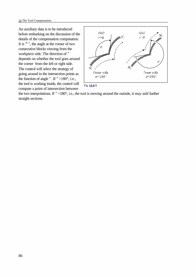
14 The Tool Compensation
86
Fig. 14.4-5
An auxiliary data is to be introducedbefore embarking on the discussion of thedetails of the compensation computation.It is """, the angle at the corner of twoconsecutive blocks viewing from theworkpiece side. The direction of "depends on whether the tool goes aroundthe corner from the left or right side.The control will select the strategy ofgoing around in the intersection points asthe function of angle ". If ">180°, i.e.,the tool is working inside, the control willcompute a point of intersection betweenthe two interpolations. If "<180°, i.e., the tool is moving around the outside, it may add furtherstraight sections.
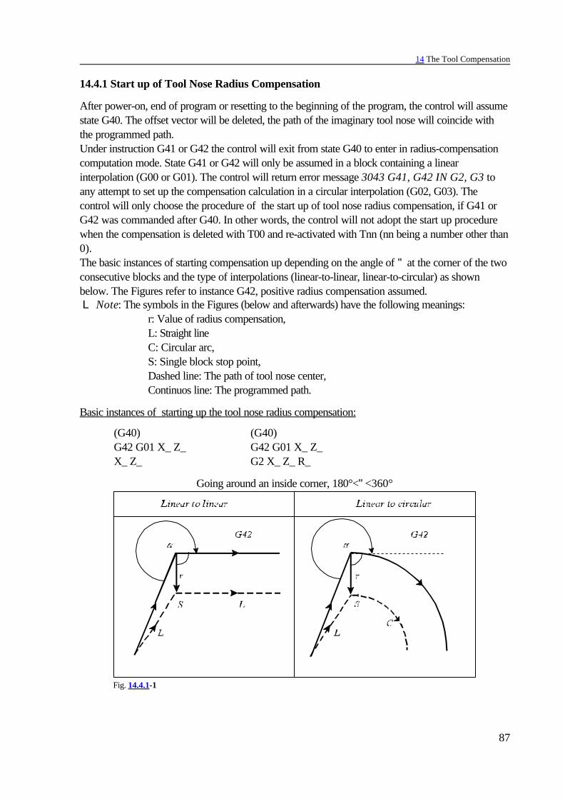
14 The Tool Compensation
87
Fig. 14.4.1-1
14.4.1 Start up of Tool Nose Radius Compensation
After power-on, end of program or resetting to the beginning of the program, the control will assumestate G40. The offset vector will be deleted, the path of the imaginary tool nose will coincide withthe programmed path.Under instruction G41 or G42 the control will exit from state G40 to enter in radius-compensationcomputation mode. State G41 or G42 will only be assumed in a block containing a linearinterpolation (G00 or G01). The control will return error message 3043 G41, G42 IN G2, G3 toany attempt to set up the compensation calculation in a circular interpolation (G02, G03). Thecontrol will only choose the procedure of the start up of tool nose radius compensation, if G41 orG42 was commanded after G40. In other words, the control will not adopt the start up procedurewhen the compensation is deleted with T00 and re-activated with Tnn (nn being a number other than0).The basic instances of starting compensation up depending on the angle of " at the corner of the twoconsecutive blocks and the type of interpolations (linear-to-linear, linear-to-circular) as shownbelow. The Figures refer to instance G42, positive radius compensation assumed. L Note: The symbols in the Figures (below and afterwards) have the following meanings:
r: Value of radius compensation,L: Straight lineC: Circular arc,S: Single block stop point,Dashed line: The path of tool nose center,Continuos line: The programmed path.
Basic instances of starting up the tool nose radius compensation:
(G40) (G40)G42 G01 X_ Z_ G42 G01 X_ Z_X_ Z_ G2 X_ Z_ R_
Going around an inside corner, 180°<"<360°

14 The Tool Compensation
88
Fig. 14.4.1-2
Fig. 14.4.1-3
Fig. 14.4.1-4
Going around the outside of a corner at an obtuse angle, 90°#"#180°
Going around the outside of a corner at an acute angle, 0°#"<90°
Special instances of starting up the radius compensation:
If values are assigned to I, J, K in the compensation-selecting block (G41 or G42) - but only to those inthe selected plane (e.g., to I, K in the case of G18) -the control will move to the intersection point betweenthe next block and the straight line defined by I, J, Kwith starting up radius compensation. The values of I,J, K are always incremental ones, the vector definedby them pointing to the end point of the interpolation,in which it has been programmed. This facility isuseful, e.g., in moving to an inside corner.

14 The Tool Compensation
89
Fig. 14.4.1-5
Fig. 14.4.1-6
Fig. 14.4.1-7
...G91 G18 G40...N110 G42 G1 X120 Z–80 I70 K50N120 Z100 ...
In this case the control will always compute a point ofintersection regardless of whether an inside or an outsidecorner is to be machined.
Unless a point of intersection is found, the control will move,at right angles, to the start point of the next interpolation.
When the compensation is set up by a special block in which no movement is programmed in theselected plane, the compensation will be set up without any movement, the calculated compensationvector’s length is 0. The compensation vector is computed at the end of the next motion blockaccording to the strategy corresponding to compensation computation in offset mode (see the nextchapter).
...N10 G40 G18 G0 X0 Z0N15 G42 N20 G1 Z80N25 X120 Z110...
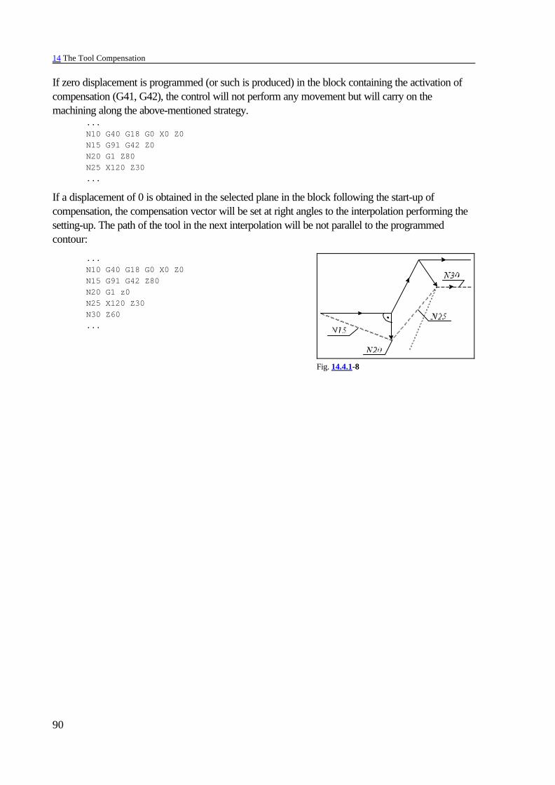
14 The Tool Compensation
90
Fig. 14.4.1-8
If zero displacement is programmed (or such is produced) in the block containing the activation ofcompensation (G41, G42), the control will not perform any movement but will carry on themachining along the above-mentioned strategy.
...N10 G40 G18 G0 X0 Z0N15 G91 G42 Z0N20 G1 Z80N25 X120 Z30...
If a displacement of 0 is obtained in the selected plane in the block following the start-up ofcompensation, the compensation vector will be set at right angles to the interpolation performing thesetting-up. The path of the tool in the next interpolation will be not parallel to the programmedcontour:
...N10 G40 G18 G0 X0 Z0N15 G91 G42 Z80N20 G1 z0N25 X120 Z30N30 Z60...

14 The Tool Compensation
91
Fig. 14.4.2-1
14.4.2 Rules of Tool Nose Radius Compensation in Offset Mode
In offset mode the compensation vectors will be calculated continuously between interpolationblocks G00, G01, G02, G03 (see the basic instances) until more than one block will be inserted,that do not contain displacements in the selected plane. This category includes a block containingdwell or functions.
Basic instances of offset mode:
Computation of intersection point for inside corners, 180°<"<360°
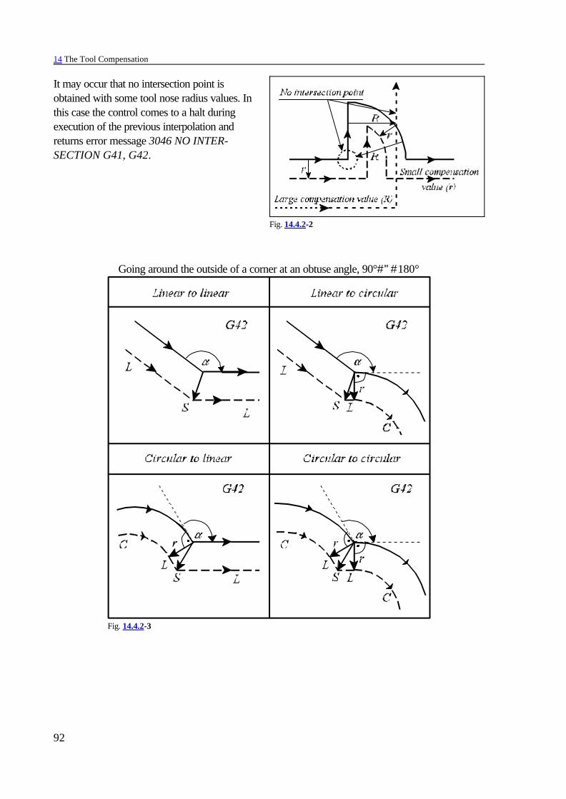
14 The Tool Compensation
92
Fig. 14.4.2-2
Fig. 14.4.2-3
It may occur that no intersection point isobtained with some tool nose radius values. Inthis case the control comes to a halt duringexecution of the previous interpolation andreturns error message 3046 NO INTER-SECTION G41, G42.
Going around the outside of a corner at an obtuse angle, 90°#"#180°

14 The Tool Compensation
93
Fig. 14.4.2-4
Fig. 14.4.2-5
Going around the outside of a corner at an acute angle, 0°#"<90°
Special instances of offset mode:
If zero displacement is programmed (or such is obtained) in the selected plane in a block in offsetmode, a perpendicular vector will be positioned to the end point of the previous interpolation, thelength of the vector will be equal to the radius value. Instances of this kind should be handled withcaution because of the hazards of inadvertent undercutting or distortions (in the case of a circle). For example:
...G91 G18 G42...N110 G1 X100 Z40N120 Z0N130 Z90N140 X–40 Z50...

14 The Tool Compensation
94
Fig. 14.4.3-1
Fig. 14.4.3-2
14.4.3 Canceling of Offset Mode
Command G40 will cancel the computation of tool radius compensation. Such a command can beissued with linear interpolation only. The control will return error message 3042 G40 IN G2, G3 toany attempt to program G40 in a circular interpolation.
Basic instances of canceling offset mode:
(G42) (G42)G01 X_ Z_ G02 X_ Z_ R_G40 X_ Z_ G40 G1 X_ Z_
Going around an inside corner, 180°<"<360°
Going around the outside of a corner at an obtuse angle, 90°#"#180°
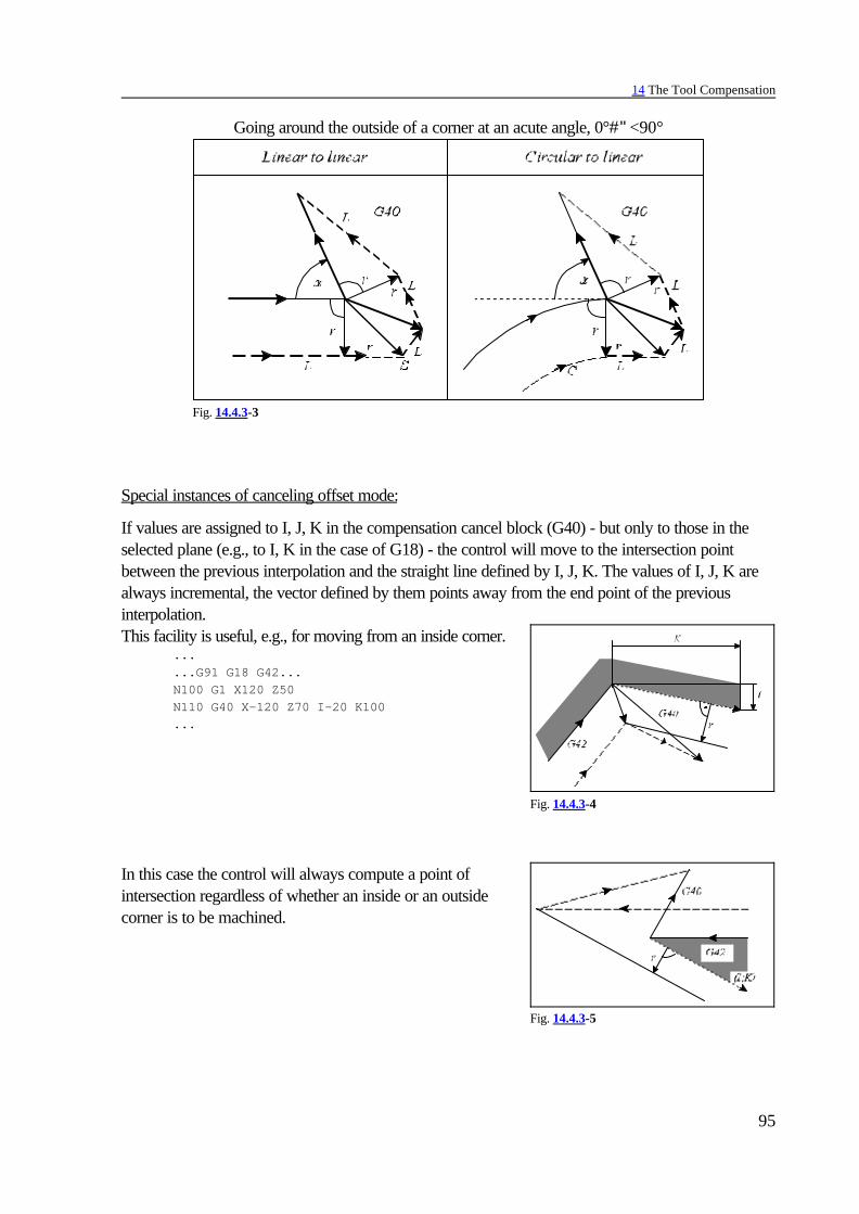
14 The Tool Compensation
95
Fig. 14.4.3-3
Fig. 14.4.3-4
Fig. 14.4.3-5
Going around the outside of a corner at an acute angle, 0°#"<90°
Special instances of canceling offset mode:
If values are assigned to I, J, K in the compensation cancel block (G40) - but only to those in theselected plane (e.g., to I, K in the case of G18) - the control will move to the intersection pointbetween the previous interpolation and the straight line defined by I, J, K. The values of I, J, K arealways incremental, the vector defined by them points away from the end point of the previousinterpolation. This facility is useful, e.g., for moving from an inside corner.
...
...G91 G18 G42...N100 G1 X120 Z50 N110 G40 X–120 Z70 I–20 K100...
In this case the control will always compute a point ofintersection regardless of whether an inside or an outsidecorner is to be machined.

14 The Tool Compensation
96
Fig. 14.4.3-6
Fig. 14.4.3-7
Fig. 14.4.3-8
Unless a point of intersection is found, the control will move,at a right angle, to the end point of the previous interpolation.
If the compensation is canceled in a block in which nomovement is programmed in the selected plane, an offsetvector perpendicular to the end point of the previousinterpolation will be set and the compensation vector will bedeleted by the end of the next movement block.
...G42 G18 G91...N110 G1 X80 Z80N120 G40N130 X40 Z–70...
If zero displacement has been programmed (or such isobtained) in the block (G40) in which the compensation iscanceled, an offset vector perpendicular to the end point ofthe previous interpolation will be calculated, and the controlwill cover that instance in block G40. For example:
...G42 G18 G91...N110 G1 X80 Z80N120 G40 X0N130 X40 Z–70...
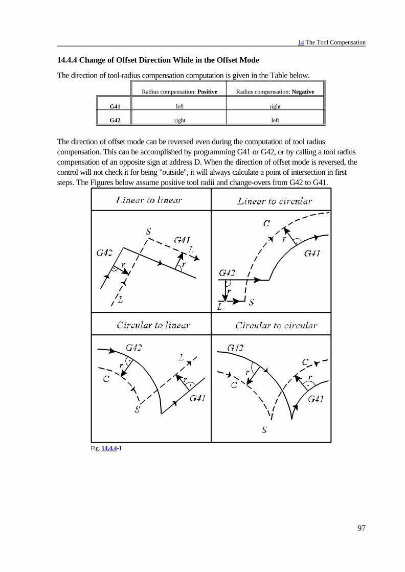
14 The Tool Compensation
97
Fig. 14.4.4-1
14.4.4 Change of Offset Direction While in the Offset Mode
The direction of tool-radius compensation computation is given in the Table below.
Radius compensation: Positive Radius compensation: Negative
G41 left right
G42 right left
The direction of offset mode can be reversed even during the computation of tool radiuscompensation. This can be accomplished by programming G41 or G42, or by calling a tool radiuscompensation of an opposite sign at address D. When the direction of offset mode is reversed, thecontrol will not check it for being "outside", it will always calculate a point of intersection in firststeps. The Figures below assume positive tool radii and change-overs from G42 to G41.

14 The Tool Compensation
98
Fig. 14.4.4-2
Fig. 14.4.4-3
Fig. 14.4.4-4
Unless a point of intersection is found in alinear-to-linear transition, the path of the toolwill be:
Unless a point of intersection is found in alinear-to-circular transition, the path of the toolwill be:
Unless a point of intersection is obtained in acircular-to-linear or circular-to-circulartransition, the end of compensation vector in thestart point of the first circular interpolation willbe connected with the end point of thecompensation vector perpendicular to the startpoint of the second interpolation by a circulararc of uncorrected programmed radius R. Nowthe center of the interconnecting circular arc willnot coincide with the center of the programmedarc. The control will return error message 3047CHANGE NOT POSSIBLE if the directionchange is not feasible even with the relocation ofthe circle center outlined above.

14 The Tool Compensation
99
Fig. 14.4.5-1
Fig. 14.4.5-2
14.4.5 Programming Vector Hold (G38)
Under the action of commandG38 v
the control will hold the last compensation vector between the previous interpolation and G38 blockin offset mode, and will implement it at the end of G38 block irrespective of the transition betweenthe G38 block and the next one. Code G38 is a single-shot one, i.e., it will not be modal. G38 has to be programmed over again if the vector is to be held in several consecutive blocks.G38 can be programmed in state G00 or G01 only, i.e., the vector-hold block must be invariably alinear interpolation, or else the control will return error message 3040 G38 NOT IN G0, G1. Unlesscode G38 is used in offset mode (G41, G42), the control will return error message 3039 G38CODE IN G40.An example of using G38:
...G18 G41 G91...N110 G1 X120 Z60N120 G38 X–80 Z90N130 X140 Z20N140 Z120...
To program a recession without canceling theoffset mode:
...G18 G42 G91...N110 G1 Z40N120 G38 Z50N130 G38 X140N140 G38 X-140N150 Z60...
14.4.6 Programming Corner Arcs (G39)
By programmingG39 (I J K),
it will be possible - in offset mode - to avoid the automatic intersection-point computation or theinsertion of linear sections when going around outside corners, instead the tool center will travelalong a circular arc equal to the tool radius.It will insert an arc equal to the tool radius in direction G02 or G03 in state G41 or G42,respectively.

14 The Tool Compensation
100
Fig. 14.4.6-1
Fig. 14.4.6-2
The start and end points of the arc will be givenby a tool-radius long vector perpendicular to theend point of the path of previous interpolationand by a tool-radius vector perpendicular to thestart point of the next one, respectively. G39has to be programmed in a separate block:
...G18 G91 G41...N110 G1 Z100N120 G39N130 G3 X–160 Z80 K80...
When I, J or K is programmed in block G39,the end point of the circular arc will be given bya tool-radius long vector perpendicular to thevector defined by I, J or K from the end pointof the previous interpolation, in accordance withthe selected plane.
...G18 G91 G41...N110 G1 Z100N120 G39 I–60 K50N130 G40 X60 Z110...
The previously selected mirroring or rotating commands are effectual the vector defined by I, J or K.As a matter of fact, the scaling command will not affect the direction. No movement command canbe programmed in a block of G39 type. The control will return error message 3036 G39 CODE ING40 if command G39 is issued in state G40 or 3D compensation mode.

14 The Tool Compensation
101
Fig. 14.4.7-1
Fig. 14.4.7-2
14.4.7 General Information on Tool Nose Radius Compensation
In offset mode (G41, G42), the control will always have to compute the compensation vectorsbetween two interpolation blocks in the selected plane. In practice it may be necessary to programbetween two interpolation blocks in the selected plane a non-interpolation block or an interpolationoutside of the selected plane. They may be – functions (M, S, T) – dwell (G4 P) – interpolation outside of the selected plane (G18) G1 Y – call of a subprogram (M98 P) – setting or canceling special transformations (G50, G51, G50.1, G51.1, G68, G69).
L Note: Calling a subprogram some carefulness is needed. Unless the subprogram is beginningwith a motion command in the assigned plane, the interpolation will be distorted.
The control will accept the programming of a single blockof the above type between two interpolation blocks in theprogram, leaving the path of the tool unaffected:
...G18 G42 G91...N110 G1 X140 Z50N120 G4 P2N130 Z60...
When the control inserts one or more straight lines between two interpolations when goingaround a corner, any other block without movement or with movement outside of the selectedplane programmed between the interpolations will be executed at the single block stop point(indicated by "S" in the figures).
When two interpolations outside of the selected planeor two blocks containing no interpolations are writtenin the program, the control will set an offset vectorperpendicular to the end point of the last interpolationin the selected plane and the path will be distorted:
...G18 G42 G91...N110 G1 X140 Z50N120 G4 P2N130 S400N140 Z60...

14 The Tool Compensation
102
Fig. 14.4.7-3
Fig. 14.4.7-4
Fig. 14.4.7-5
If no cut is feasible in direction Y unless the radius compensation is setup, the following procedure may be adopted:
...G18 G91...N110 G41 G0 X140 Z50 N120 G1 Y-40N130 X80...
Now the tool will have a correct path as is shown in the Figure.
If, however, movement in direction Y is broken up into two sections(rapid traverse and feed), the path will be distorted because of thetwo consecutive interpolations outside of the selected plane:
...G18 G91...N110 G41 G0 X140 Z50N120 Y-35N130 G1 Y-5N140 X80...
As a trade-off, insert a small movement in direction X between twoones in direction Y:
...G18 G91...N110 G41 G0 X1380 Z50N120 Y-35N130 X2N140 G1 Y-5N150 X80...
With the above "trick" a correct compensation vector can be got.

14 The Tool Compensation
103
Fig. 14.4.7-6
Fig. 14.4.7-7
The path of tool will be as follows when instructionsG22, G23, G52, G54-G59, G92G53G28, G29, G30
are inserted between two interpolations.When command G22, G23, G52, G54-G59 or G92 is programmed in offset mode between twointerpolation blocks, the compensation vector will be deleted at the end point of the previousinterpolation, the command will be executed and the vector will be restored at the end point of thenext interpolation. If the previous or next interpolation is a circular one, the control will return errormessage 3041 AFTER G2, G3 ILLEG. BLOCK. For example:...G91 G18 G41...N110 G1 X–100 Z80N120 G92 X0 Z0N130 X100 Z80...
If command G53 is programmed in offset mode between two interpolations, the compensationvector will be deleted at the end point of the previous block, the positioning will be executed in G53,and the vector will be restored at the end point of the next interpolation (other than G53). If theprevious or next interpolation is a circular one, the control will return error message 3041 AFTERG2, G3 ILLEG. BLOCK. For example: ...G91 G18 G41...N110 G1 X–100 Z80N120 G53 X1600N130 G53 X0N140 X100 Z80...

14 The Tool Compensation
104
Fig. 14.4.7-8
Fig. 14.4.7-9
If G28 or G30 is programmed (followed by G29) between two blocks in offset mode, thecompensation vector will be deleted at the end point of the block it positions the tool to theintermediate point, the tool will move to the reference point, and the vector will be restored at theend point of the returning block G29. For example:...G91 G18 G41...N110 G1 X–100 Z80N120 G28 X160N130 G29 X0N140 X100 Z80...
A new compensation value can also becalled at address T in offset mode. In theevent of a reversal in the sign of theradius, the direction of motion along thecontours will be reversed (see earlier).Otherwise, the following procedure willbe applicable. The compensation vectorwill be calculated with the new radiusvalue at the end point of the interpolation,in which the new address T has beenprogrammed. Since the compensation vector has been computed with the previous radius value atthe start point of that block, the path of the tool center will not be parallel to the programmed path.A new radius compensation value can be called at address T in a circular interpolation, too, thistime, however, the tool center will be moving along an arc with a variable radius.A special instance of the foregoing is canceling or setting up the compensation with T00 or Tnn,respectively, while in offset mode. Notice the difference in tool paths with reference to the followingexample, when the compensation is set up with G41 or G42 and canceled with G40, or when thecompensation is set up and canceled by programming T.

14 The Tool Compensation
105
Fig. 14.4.7-10
Fig. 14.4.7-11
Fig. 14.4.7-12
A particular program detail or subprogram may be used also for machining a male or female work-piece with positive or negative radius compensation, respectively, or vice-versa. Let us review the following small programdetail:
...N020 G42 G1 X160 T1N030 G1 Z-5N040 G3 I-80N050 G1 Z2N060 G40 G0 X0...
When the radius compensation is applied to acircle of a variable radius, the control willcalculate the compensation vector(s) to animaginary circle at the start point thereof, theradius of which is equal to the start-point radiusof the programmed circle, the center pointcoinciding with the programmed one. Thecompensation vector(s) will be computed to animaginary circle at the end point of it, the radiusof which is equal to the end-point radius of the programmed circle, the center point coinciding withthat of the programmed circle.

14 The Tool Compensation
106
Fig. 14.4.7-13
Fig. 14.4.7-14
When a full circle is being programmed, it may often occur that the path of tool covers more than acomplete revolution round the circle in offset mode.For example, this may occur in programming a directionreversal along the contours:
...G17 G42 G91...N110 G1 X30 Y-40N120 G41 G2 J-40N130 G42 G1 X30 Y40...
The tool center covers a full arc of a circle from point P1 topoint P1 and another one from point P1 to point P2.
When offset mode is canceled by programming I, J, K, asimilar condition will emerge:
...G18 G90 G41...N090 G1 Z60N100 G2 I-60N110 G40 G1 X360 Z120 I-60 K-60...
The tool center covers a full arc of a circle from point P1 topoint P1 and another one from point P1 to point P2.

14 The Tool Compensation
107
Fig. 14.4.7-15
Fig. 14.4.8-1
Two or more compensation vectors may be producedwhen going around sharp corners. When their endpoints lie close to each other, there will be hardly anymotion between the two points.When the distance between the two vectors is smallerthan the value of parameter DELTV in each axis, thevector shown in the Figure will be omitted, and thepath of the tool will be modified accordingly.
L Note: When parameter DELTV is too high (incauseless way) the sharp corners with acuteangles may be overcut.
14.4.8 Interferences in Tool Nose Radius Compensation
It may frequently occur in offset mode that the path of the tool is the opposite of the programmedone. Under such conditions, the tool may cut into the workpiece contrary to the programmer'sintentions. This phenomenon is referred to as the interference in tool nose radius compensation.
In the case shown in the Figure, after the intersection pointshave been computed, a tool path opposite to theprogrammed one will be obtained in the execution ofinterpolation N2. The hachure area indicates that the toolcuts in the workpiece.
To avoid this, the control performs an interference check when parameter INTERFER is set to 1.Now the control will check that the condition -90°#n#+90° is fulfilled for angle n between theprogrammed displacement and the one compensated with the radius.

14 The Tool Compensation
108
Fig. 14.4.8-2
Fig. 14.4.8-3
In the other words thecontrol will check wether thecompensated displacementvector has a componentopposite to the programmeddisplacement vector or not.
If parameter ANGLAL is set to 1, the control will, after an angle check, return an interference errormessage 3048 INTERFERENCE ALARM one block earlier than the occurrence of the trouble.

14 The Tool Compensation
109
Fig. 14.4.8-4
If parameter ANGLAL is set to 0, the control will not return an error message, but will automaticallyattempt to correct the contour in order to avoid overcutting. The procedure of compensation is asfollows.Each of blocks A, B and C are in offset mode. The computed vectors between blocks A and B areLP1, LP2, LP3, LP4; the compensation vectors between blocks B and C are LP5, LP6, LP7, LP8.
- LP4 and LP5 will be ignored if there is an interference between them.- LP3 and LP6 will be ignored if there is an interference between them.- LP2 and LP7 will be ignored if there is an interference between them.- LP1 and LP8 cannot be omitted in the case of an interference, so an error message is
returned.
It is evident from the foregoing that the compensation vectors are paired at the start and end pointsof interpolation B, and will be ignored in pairs. If the number of compensation vectors on one side is1 (or is reduced to 1), only the vectors on the other side will be omitted. The procedure of omittingwill be carried on as long as the interference persists. The first compensation vector at the start pointof interpolation B and the last one at the respective end point cannot beignored. If, as a result ofomissions, the interference is eliminated, no error message will be returned, but error message 3048INTERFERENCE ALARM will be returned otherwise. The remaining compensation vectors aftereach omission will always be interconnected by straight lines - even if interpolation B has been acircular one.It is evident from the above example that the execution of interpolation A will not be commencedunless interpolation B has been checked for an interference. To do so, however, block C also hadto be entered in the buffer, and the compensation vectors had to be calculated for transition B - C.
A few typical instances of interference will be described below.
Cutting a step smaller than the tool radius.The control returns error message 3048INTERFERENCE ALARM or else itwould cut in the workpiece.

14 The Tool Compensation
110
Fig. 14.4.8-5
Fig. 14.4.8-6
Fig. 14.4.8-7
Machining an inside corner with a radius smaller thanthe tool radius. The control returns error message3048 INTERFERENCE ALARM or else overcutting would occur.
Cutting a step smaller than the tool radiusalong an arc. If parameter ANGLAL is 0,the control will delete vector LP2 and willinterconnect vectors LP1 and LP3 by astraight line to avoid a cut-in. If parameterANGLAL is 1 it returns error message3048 INTERFERENCE ALARM andstops at the end of previous block.
Sometimes the tool would not actually overcut the workpiece, but the interference check indicatesan error.If a recess smaller than the radius compensationis being machined, actually no overcut wouldoccur (see the Figure), yet the control returnserror message 3048 INTERFERENCEALARM because the direction of displacementalong the compensated path in interpolation B isopposite to the programmed one.

14 The Tool Compensation
111
Fig. 14.4.8-8
In the above example an interference error isreturned again because the displacement of thecompensated path in interpolation B is oppositeto the programmed one.
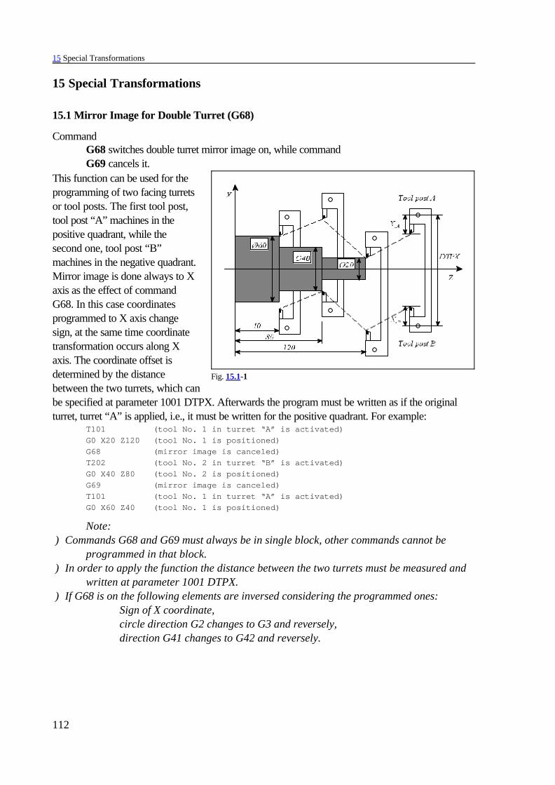
15 Special Transformations
112
Fig. 15.1-1
15 Special Transformations
15.1 Mirror Image for Double Turret (G68)
Command G68 switches double turret mirror image on, while commandG69 cancels it.
This function can be used for theprogramming of two facing turretsor tool posts. The first tool post,tool post “A” machines in thepositive quadrant, while thesecond one, tool post “B”machines in the negative quadrant.Mirror image is done always to Xaxis as the effect of commandG68. In this case coordinatesprogrammed to X axis changesign, at the same time coordinatetransformation occurs along Xaxis. The coordinate offset isdetermined by the distancebetween the two turrets, which canbe specified at parameter 1001 DTPX. Afterwards the program must be written as if the originalturret, turret “A” is applied, i.e., it must be written for the positive quadrant. For example:
T101 (tool No. 1 in turret “A” is activated)G0 X20 Z120 (tool No. 1 is positioned)G68 (mirror image is canceled)T202 (tool No. 2 in turret “B” is activated)G0 X40 Z80 (tool No. 2 is positioned)G69 (mirror image is canceled)T101 (tool No. 1 in turret “A” is activated)G0 X60 Z40 (tool No. 1 is positioned)
Note: ) Commands G68 and G69 must always be in single block, other commands cannot be
programmed in that block. ) In order to apply the function the distance between the two turrets must be measured and
written at parameter 1001 DTPX. ) If G68 is on the following elements are inversed considering the programmed ones:
Sign of X coordinate,circle direction G2 changes to G3 and reversely,direction G41 changes to G42 and reversely.

15 Special Transformations
113
Fig. 15.2-1
Fig. 15.2-2
15.2 Scaling (G50, G51)
CommandG51 v P
can be used for scaling a programmed shape.P1...P4: Points specified in the part programP1'...P4': Points after scalingP0: Center of scalingThe coordinates of the scaling center can be entered atcoordinates of v. The applicable addresses are X, Y, Z, U,V, W. The coordinate data of v entered here will also beinterpreted as rectangular (Cartesian) data, even when thepolar coordinate data specification is set up.Using G90, G91 or operator I, the v coordinates of thecenter of scaling can be specified as absolute or incrementaldata.Unless one or both axes’ addresses are assigned values, theinstantaneous axis position will be taken for the center ofscaling.The scale factor can be specified at address P. Its value can be represented by 8 decimal digits; theposition of the decimal point is irrelevant.Scaling can be canceled with command
G50.For example:
N1 G90 G0 X100 Z120N2 G51 X0 Z0 P0.5N3 G1 X0 Z100 F150N4 X80N5 Z0N6 G50 N7 G0 X100 Z120
15.3 Programmable Mirror Image (G50.1, G51.1)
A programmed shape can be projected as a mirror image along the coordinates selected in v bycommand
G51.1 v

15 Special Transformations
114
Fig. 15.3-1
in such a way that the coordinates of the axis (or axes) of mirror image can be specified in v. The vcoordinate may be X, Y, Z, U, V, W, A, B, C.The v coordinate data entered here are interpreted as rectangular coordinate data even when polarcoordinate data specifications are set up.Using G90, G91 or operator I, the v coordinates of the axes of the mirror image can be specified asabsolute or incremental data.No mirror image will be on the axis, for the address of which no value has been assigned.
CommandG50.1 v
will cancel the mirror image on axis (axes) specified at v. Any arbitrary data can be written for the vcoordinates, its effect will only record the fact of canceling.When this command is issued, no rotation or scaling command may be in effect. Otherwise an errormessage 3000 MIRROR IMAGE IN G51, G68 is returned.When a mirror image is applied on an axis of composing the selected plane: – The circle direction is reversed automatically (interchange of G02, G03) – The angle of rotation is assigned an opposite meaning (G68).
Example:
SubprogramO0101N1 G0 X40 F120N2 G1 Z80N3 G3 X80 Z100 R20N4 G1 X100 Z110N5 M99
main program
O0100N10 T101N20 G0 X160 Z60 M3 S1000N30 M98 P101 (subprogram call)N40 G0 X160 Z120N50 T202N60 G0 X160 Z60 M3 S1000N70 G51.1 Z60 (mirror image parallel to X, coordinate Z=60)N80 M98 P101 (subprogram call)N90 G50.1 Z0 (canceling mirror image parallel to X)N100 G0 X160 Z120N110 M30
The mirror image can only be switched on in state G50, i.e., if the scaling command is not active.However, in the switched-on state of the mirror image the scaling can also be switched on. It is alsotrue for the mirror image that it cannot be overlapped with scaling command, i.e., first the scaling has

15 Special Transformations
115
to be canceled and only then the cancellation of the mirror image may come:G51.1 ... (mirror image on) G51 ... (scaling on)...G50 ... (scaling off)G50.1 ... (mirror image off)

16 Automatic Geometric Calculations
116
Fig. 16.1-1
Fig. 16.1-2
16 Automatic Geometric Calculations
16.1 Programming Chamfer and Corner Round
The control is able to insert chamfer or rounding between two blocks containing linear (G01) orcircle interpolation (G02, G03) automatically.A chamfer, the length of whichequals to the value specified ataddress
,C(comma and C) is insertedbetween the end point of the blockcontaining address ,C and the startpoint of the forthcoming block.E.g.:N1 G1 G91 Z30 ,C10N2 X80 Z10
The value specified at the address,C shows the distance between the start/end point of chamfer and the supposed intersection of thetwo successive blocks. A chamfer may also be inserted between circles or between a circle and astraight line. In this case value ,C is the length of the chord drawn from intersection.A rounding, the radius of whichcorresponds to the value given ataddress
,R(comma and R) is insertedbetween the end point of the blockcontaining address ,R and the startpoint of the forthcoming block.E.g.:
N1 G91 G01 Z30 ,R8N2 G03 X60 Z–30 R30
A ,R-radius arc is inserted between the two blocks so that the circle osculates to both pathelements.
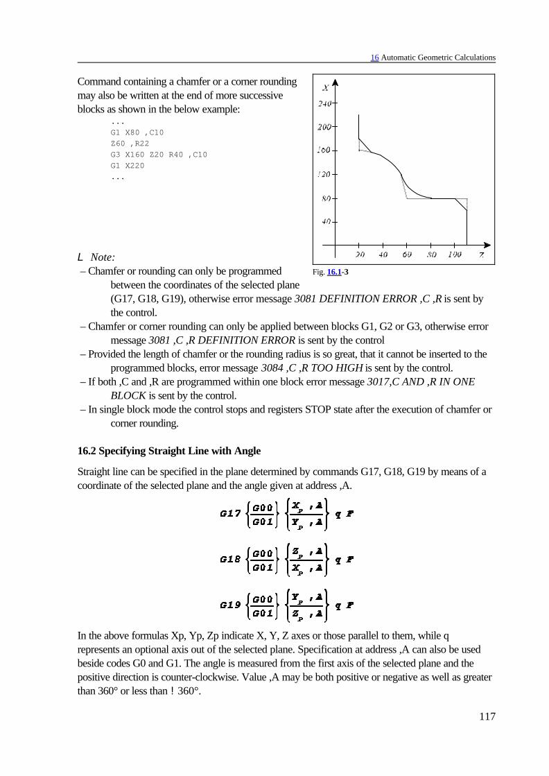
16 Automatic Geometric Calculations
117
Fig. 16.1-3
Command containing a chamfer or a corner roundingmay also be written at the end of more successiveblocks as shown in the below example:
...G1 X80 ,C10Z60 ,R22G3 X160 Z20 R40 ,C10G1 X220...
L Note: – Chamfer or rounding can only be programmed
between the coordinates of the selected plane(G17, G18, G19), otherwise error message 3081 DEFINITION ERROR ,C ,R is sent bythe control.
– Chamfer or corner rounding can only be applied between blocks G1, G2 or G3, otherwise errormessage 3081 ,C ,R DEFINITION ERROR is sent by the control
– Provided the length of chamfer or the rounding radius is so great, that it cannot be inserted to theprogrammed blocks, error message 3084 ,C ,R TOO HIGH is sent by the control.
– If both ,C and ,R are programmed within one block error message 3017,C AND ,R IN ONEBLOCK is sent by the control.
– In single block mode the control stops and registers STOP state after the execution of chamfer orcorner rounding.
16.2 Specifying Straight Line with Angle
Straight line can be specified in the plane determined by commands G17, G18, G19 by means of acoordinate of the selected plane and the angle given at address ,A.
In the above formulas Xp, Yp, Zp indicate X, Y, Z axes or those parallel to them, while qrepresents an optional axis out of the selected plane. Specification at address ,A can also be usedbeside codes G0 and G1. The angle is measured from the first axis of the selected plane and thepositive direction is counter-clockwise. Value ,A may be both positive or negative as well as greaterthan 360° or less than !360°.

16 Automatic Geometric Calculations
118
Fig. 16.2-2
Fig. 16.2-1
Fig. 16.2-3
L Note: ) In case the coordinate system is situated like on the figure beside
the interpretation of angle is modified as seen in theenclosed figure (positive direction is clockwise).
For example:(G18 G90) G1 X60 Z120 ... Z70 ,A150 (this specification is
equivalent to X117.735 Z70)X180 ,A135 (this specification is
equivalent to X180 Z38.868)
L Note: – Straight line with angle together with chamfer or
corner rounding can be defined in one block.For example:
Z100 ,A30 ,C5X100 ,A120 ,R10Z-100 ,A210
– Angle specification at address ,A can also beapplied in drilling cycles. In this case it isacknowledged in the course of positioning execution in the selected plane.For example block
G81 G91 X100 ,A30 R-2 Z-25
is equivalent to the block below:G81 G91 X100 Y57.735 R-2 Z-25
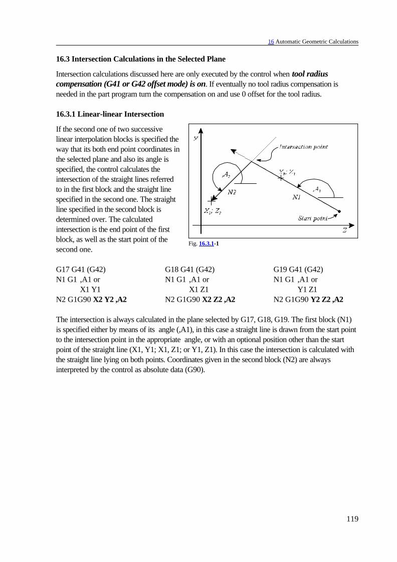
16 Automatic Geometric Calculations
119
Fig. 16.3.1-1
16.3 Intersection Calculations in the Selected Plane
Intersection calculations discussed here are only executed by the control when tool radiuscompensation (G41 or G42 offset mode) is on. If eventually no tool radius compensation isneeded in the part program turn the compensation on and use 0 offset for the tool radius.
16.3.1 Linear-linear Intersection
If the second one of two successivelinear interpolation blocks is specified theway that its both end point coordinates inthe selected plane and also its angle isspecified, the control calculates theintersection of the straight lines referredto in the first block and the straight linespecified in the second one. The straightline specified in the second block isdetermined over. The calculatedintersection is the end point of the firstblock, as well as the start point of thesecond one.
G17 G41 (G42)N1 G1 ,A1 or
X1 Y1N2 G1G90 X2 Y2 ,A2
G18 G41 (G42)N1 G1 ,A1 or
X1 Z1N2 G1G90 X2 Z2 ,A2
G19 G41 (G42)N1 G1 ,A1 or
Y1 Z1N2 G1G90 Y2 Z2 ,A2
The intersection is always calculated in the plane selected by G17, G18, G19. The first block (N1)is specified either by means of its angle (,A1), in this case a straight line is drawn from the start pointto the intersection point in the appropriate angle, or with an optional position other than the startpoint of the straight line (X1, Y1; X1, Z1; or Y1, Z1). In this case the intersection is calculated withthe straight line lying on both points. Coordinates given in the second block (N2) are alwaysinterpreted by the control as absolute data (G90).

16 Automatic Geometric Calculations
120
Fig. 16.3.1-2
For example:(G18) G90 G41 ...G0 X20 Z90N10 G1 ,A150N20 X40 Z10 ,A225G0 Z0...
Block N10 can also be given with thecoordinates of a point of the straight line:
(G18) G90 G41 ...G0 X20 Z90N10 G1 X66.188 Z50N20 X40 Z10 ,A225G0 X0 Y20...
Note, that in this case coordinate X, Z (X66.18 Z50) given in block N10 is not acknowledged bythe control as end point, but as a transit position binding the straight line with the start point.

16 Automatic Geometric Calculations
121
Fig. 16.3.1-3 Fig. 16.3.1-4
Intersection calculation can also be combined with a chamfer or corner rounding specification. E.g.:
(G18) G90 G41 ...G0 X20 Z90N10 G1 X66.188 Z50 ,C10N20 X40 Z10 ,A225G0 X0 Y20...
(G18) G90 G41 ...G0 X20 Z90N10 G1 X66.188 Z50 ,R10N20 X40 Z10 ,A225G0 X0 Y20...
In the above examples chamfering amount is measured from the calculated intersection, as well asrounding is inserted to the calculated intersection.

16 Automatic Geometric Calculations
122
16.3.2 Linear-circular Intersection
If a circular block is given after a linear block in a way that the end and center position coordinatesas well as the radius of the circle are specified, i.e., the circle is determined over, then the controlcalculates intersection between straight line and circle. The calculated intersection is the end point ofthe first block, as well as the start point of the second one.

16 Automatic Geometric Calculations
123
Fig. 16.3.2-1 Fig. 16.3.2-2
G17 G41 (G42)N1 G1 ,A or
X1 Y1N2 G2 (G3) G90 X2 Y2 IJ R Q
G18 G41 (G42)N1 G1,A or
X1 Z1N2 G2 (G3) G90 X2 Z2 IK R Q
G19 G41 (G42)N1 G1 ,A or
Y1 Z1N2 G2 (G3) G90 Y2 Z2 JK R Q
The intersection is always calculated in the plane selected by G17, G18, G19. The first block (N1)is specified either by means of its angle (,A), in this case a straight line is drawn from the start pointto the intersection point in the appropriate angle, or an optional point other than the start point of thestraight line is given (X1, Y1; X1, Z1; or Y1, Z1). In this case the intersection is calculated with thestraight line lying on both points. Coordinates given in the second block (N2) also I, J, Kcoordinates defining the center of the arc, are always interpreted by the control as absolute data(G90). Of the two resulting intersections the one to be calculated by the control can be specified ataddress Q. If the address value is less than zero (Q<0) the nearer intersection in direction of thestraight line is calculated, while if the address value is greater than zero (Q>0) the fartherone in direction of the straight line is calculated. The direction of movement along thestraight line is determined by the angle.

16 Automatic Geometric Calculations
124
Fig. 16.3.2-3 Fig. 16.3.2-4
Let us see the following example:
%O9981N10 (G18) G42 G0 X40 Z100 S200 M3N20 G1 X-40 Z-30N30 G3 X80 Z20 I-10 K20 R50 Q-1N40 G40 G0 X120N50 Z120N60 M30%
%O9982N10 (G18) G42 G0 X40 Z100 S200 M3N20 G1 X-40 Z-30N30 G3 X80 Z20 I-10 K20 R50 Q1N40 G40 G0 X120N50 Z120N60 M30%
Circular block N30 G3 is determined over, for both the center coordinates (I–10 K20 in absolutevalue) and the circle radius (R50) are specified, the control calculates the intersection of the straightline given in block N20 and the circle given in block N30. In program O9981 the nearer intersectionin direction of the straight line is calculated because Q–1 is given in circular block N30.
Linear-circular intersection calculation can also be combined with chamfering or roundingspecification. E.g.:
%O9983N10 (G18) G42 G0 X40 Z100 S200 M3N20 G1 X-40 Z-30 ,R15N30 G3 X80 Z20 I-10 K20 R50 Q-1N40 G40 G0 X120N50 Z120N60 M30%
The control calculates the intersection of blocks N20 and N30 and inserts a 15mm corner roundingas the effect of ,R15 given in block N20.
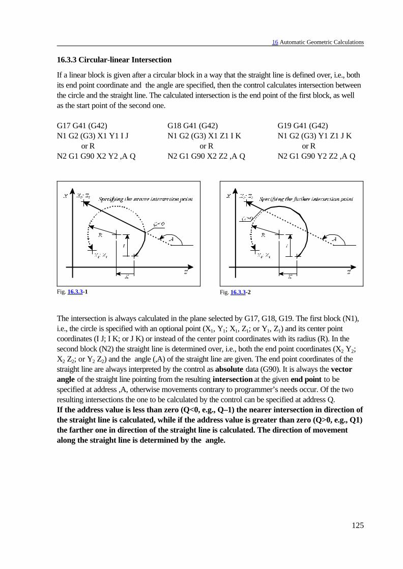
16 Automatic Geometric Calculations
125
Fig. 16.3.3-1 Fig. 16.3.3-2
16.3.3 Circular-linear Intersection
If a linear block is given after a circular block in a way that the straight line is defined over, i.e., bothits end point coordinate and the angle are specified, then the control calculates intersection betweenthe circle and the straight line. The calculated intersection is the end point of the first block, as wellas the start point of the second one.
G17 G41 (G42)N1 G2 (G3) X1 Y1 I J
or R N2 G1 G90 X2 Y2 ,A Q
G18 G41 (G42)N1 G2 (G3) X1 Z1 I K
or R N2 G1 G90 X2 Z2 ,A Q
G19 G41 (G42)N1 G2 (G3) Y1 Z1 J K or R N2 G1 G90 Y2 Z2 ,A Q
The intersection is always calculated in the plane selected by G17, G18, G19. The first block (N1),i.e., the circle is specified with an optional point (X1, Y1; X1, Z1; or Y1, Z1) and its center pointcoordinates (I J; I K; or J K) or instead of the center point coordinates with its radius (R). In thesecond block (N2) the straight line is determined over, i.e., both the end point coordinates (X2 Y2;X2 Z2; or Y2 Z2) and the angle (,A) of the straight line are given. The end point coordinates of thestraight line are always interpreted by the control as absolute data (G90). It is always the vector angle of the straight line pointing from the resulting intersection at the given end point to bespecified at address ,A, otherwise movements contrary to programmer’s needs occur. Of the tworesulting intersections the one to be calculated by the control can be specified at address Q. If the address value is less than zero (Q<0, e.g., Q–1) the nearer intersection in direction ofthe straight line is calculated, while if the address value is greater than zero (Q>0, e.g., Q1) the farther one in direction of the straight line is calculated. The direction of movementalong the straight line is determined by the angle.

16 Automatic Geometric Calculations
126
Fig. 16.3.3-3 Fig. 16.3.3-4
Let us see an example:
%O9983N10 (G18) G0 X90 X0 M3 S200N20 G42 G1 Z50N30 G3 X0 Z-50 R50N40 G1 X85.714 Z-50 ,A171.87 Q-1N50 G40 G0 X140 N60 Z90N70 M30%
%O9984N10 (G18) G0 X90 X0 M3 S200N20 G42 G1 Z50N30 G3 X0 Z-50 R50N40 G1 X85.714 Z-50 ,A171.87 Q1N50 G40 G0 X140 N60 Z90N70 M30%
Linear block N40 is defined over because both the end point coordinates (X85.714 Z–50) and the angle (,A171.87) of the straight line are specified. Therefore X0 Z–50 coordinates of the circleprogrammed in the previous block N30 are not referred to as end point coordinates, but only as apoint which is intersected by the circle and the end point is the calculated intersection. In programNo. O9983 the nearer intersection in the direction of the straight line is given (Q–1), while in O9984the farther one is specified (Q1).
Circular-linear intersection calculation can also be combined with a chamfer or roundingspecification. E.g.:
%O9983N10 (G18) G0 X90 X0 M3 S200N20 G42 G1 Z50N30 G3 X0 Z-50 R50 ,R15N40 G1 X85.714 Z-50 ,A171.87 Q-1N50 G40 G0 X140 N60 Z90N70 M30%
In the example a 15mm-rounding is programmed in block N30 (,R15). The control calculates theintersection of blocks N30 and N40 and inserts the programmed rounding to the resulting contour.

16 Automatic Geometric Calculations
127
Fig. 16.3.4-1 Fig. 16.3.4-2
16.3.4 Circular-circular Intersection
If two successive circular blocks are specified so that the end point, the center coordinates as wellas the radius of the second block are given, i.e., it is determined over the control calculatesintersection between the two circles. The calculated intersection is the end point of the first block, aswell as the start point of the second one.
G17 G41 (G42)N1 G2 (G3) X1 Y1 I1 J1
or X1 Y1 R1N2 G2 (G3) G90 X2 Y2I2 J2 R2 Q
G18 G41 (G42)N1 G2 (G3) X1 Z1 I1 K1
or X1 Z1 R1N2 G2 (G3) G90 X2 Z2 I2K2 R2 Q
G19 G41 (G42)N1 G2 (G3) Y1 Z1 J1 K1
or Y1 Z1 R1N2 G2 (G3) G90 Y2 Z2 J2K2 R2 Q
The intersection is always calculated in the plane selected by G17, G18, G19. The first block (N1)is specified either with the center coordinates (I1 J1; I1 K1; J1 K1) or with the radius (R1) of the circle.In this block the interpretation of center coordinates corresponds to the default circle specification,i.e., it is the relative distance from the start point. The coordinates given in the second block (N2), as

16 Automatic Geometric Calculations
128
I, J, K coordinates defining the circle center, are always interpreted by the control as absolutedata (G90). Of the two resulting intersections the one to be calculated by the control can bespecified at address Q. If the address value is less than zero (Q<0, e.g., Q–1) the first intersectionis calculated, while if the address value is greater than zero (Q>0, e.g., Q1) it is the second one.The first intersection is the one, first intersected going clockwise (independent of theprogrammed direction G2, G3).

16 Automatic Geometric Calculations
129
Fig. 16.3.4-3 Fig. 16.3.4-4
Let us see the following example:
%O9985N10 (G18) G0 X20 Z200 M3 S200N20 G42 G1 Z180N30 G3 X-80 Z130 R-50N40 X174.892 Z90 I30 K50 R70 Q–1N50 G40 G0 X200N60 Z200N70 M30%
%O9986N10 (G18) G0 X20 Z200 M3 S200N20 G42 G1 Z180N30 G3 X-80 Z130 R-50N40 X174.892 Z90 I30 K50 R70 Q1N50 G40 G0 X200N60 Z200N70 M30%
Circular block N40 is defined over because both, the center coordinates (I30 K50 in absolutevalue) and the radius (R70) of the circle, are specified. Therefore coordinates X–80 Z130 of thecircle programmed in the previous block N30, are not referred to as end point coordinates, but onlyas a point which is lying on the circle and the end point is the calculated intersection. In program No.O9985 the nearer intersection in clockwise direction is given (Q–1), while in O9986 the farther oneis specified (Q1).Circle intersection calculation can also be combined with chamfer or corner rounding specification.E.g.:
%O9986N10 (G18) G0 X20 Z200 M3 S200N20 G42 G1 Z180N30 G3 X-80 Z130 R-50 ,R20N40 X174.892 Z90 I30 K50 R70 Q1N50 G40 G0 X200N60 Z200N70 M30%
In the example a 20mm corner-rounding is programmed in block N30 (,R20). The controlcalculates the intersection of blocks N30 and N40 and inserts the programmed rounding to theresulting contour.

16 Automatic Geometric Calculations
130
Fig. 16.3.5-1
16.3.5 Chaining of Intersection Calculations
Intersection calculation blocks can be chained, i.e., more successive blocks can be selected forintersection calculation. The control calculates intersection till straight lines or circles determined overare found. Let us examine the example below:
%O9984N10 (G18) G0 G42 X40 Z230 F300 S500 M3N20 G1 X100 Z170N30 G3 X20 Z110 I40 K150 R50 Q-1N40 X140 Z60 I70 K100 R40 Q1N50 G1 X120 Z80 ,A135 Q1N60 X216 Z10 ,A180N70 G40 G0 X260N80 Z240N90 M30%
In the above example blocks N30, N40, N50, N60 are determined over. Linear block N20 is notdrawn to its programmed end point (X100 Z170) because circular block N30 is defined over, i.e.,addresses I, J, R are all filled in and the intersection to be searched is given at address Q. Norcircular block N30 is drawn to its programmed end point (X20 Z110) for circular block N40 is alsodetermined over. The last block determined over in the program is the linear block N60. As thefollowing linear block N70 is not defined over, coordinates X216 Z10 programmed in block N60are not referred to as an intersection point of the straight line but as end point coordinates of blockN60.
In general it is true, that the coordinate points of linear and circular blocks determined overin the selected plane are only referred to by the control as end point coordinates if they arenot followed by a block defined over.

17.1.1 Cutting Cycle (G77)
131
Fig. 17.1.1-1 Fig. 17.1.1-2
17 Canned Cycles for Turning
17.1 Single Cycles
The single cycles are the cutting cycle G77, the simple thread cutting cycle G78 and the end facecutting cycle G79.
17.1.1 Cutting Cycle (G77)
Straight cutting cycle can be defined in the following way:G77 X(U)__ Z(W)__ F__
Incremental programming is also possible with operator I or by programming G91.In case of incremental programming the data sign determines the direction of pathes Nos. 1 and 2.In the figure the sign of both addresses U and W is negative.In the block in pathes Nos. 2 and 3 the movement is at feedrate programmed at address F or at theone that is modal, while that in pathes Nos. 1 and 4 is at rapid traverse rate.
Taper cutting cycle can be defined in the following way:
G77 X(U)__ Z(W)__ R(I)__ F__
The taper can be specified at either address R or I. In both cases the data interpretation is the same.The data given at address R(I) is always incremental, and is acknowledged from the positiongiven at address X(U). The taper slope direction is determined by the sign of address R(I).The interpretation of the other addresses corresponds to those discussed earlier at straight cuttingcycle.Code G77 and data programmed in block G77 are modal.In single block mode stop is activated at the end of all four actions (1, 2, 3, 4).

17.1.1 Cutting Cycle (G77)
132
Fig. 17.1.1-3
In case of incremental programming the signs of addresses U, W and R(I) influence the movementdirections as follows:

17.1.2 Thread Cutting Cycle (G78)
133
Fig. 17.1.2-1 Fig. 17.1.2-2
17.1.2 Thread Cutting Cycle (G78)
Straight thread cutting cycle can be defined in the following way:
G78 X(U)__ Z(W)__ Q__ F(E)__
Incremental programming is also possible with operator I or by programming G91.In case of programming the data sign determines the direction of pathes Nos. 1 and 2. In the figurethe sign of both addresses U and W is negative.In the block either the thread lead is programmed at address F or the number of ridges pro inch isprogrammed at address E, as well as the thread start angle in degrees calculated from the encoderzero pulse as written in block G33.Movements Nos. 1, 3, 4 are at rapid traverse rate.At the end of path No. 2, where thread cutting occurs, approximately a 45 deg chamfering isexecuted. The chamfering amount is determined by parameter 1334 THRDCHMFR indicated with r in thefigure. The length of section is
r@L/10where r: Value of parameter THRDCHMFR
L: Programmed thread lead.The value of parameter THRDCHMFR ranges from 1 to 255, i.e. the chamfering ranges from 0.1Lto 25.5L. If for example the parameter value is 4 and the programmed thread lead is F2 then thechamfering amount: 2*(4/10)=0.8mm

17.1.2 Thread Cutting Cycle (G78)
134
Fig. 17.1.2 -3
Taper thread cutting cycle can be defined in the following way:
G78 X(U)__ Z(W)__ R(I)__ Q__ F(E)__
The taper can be specified at either address R or I. In both cases the data interpretation is the same.The data given at address R(I) is always incremental, and is acknowledged from the positiongiven at address X(U). The taper slope direction is determined by the sign of address R(I).The interpretation of the other addresses corresponds to those discussed for straight thread cuttingcycle.The chamfering angle is in this case also 45° and chamfering amount r is measured along the straightline parallel to the axes.Code G78 and data programmed in block G78 are modal.In single block mode stop is activated at the end of all four actions (1, 2, 3, 4).
Effect of STOP button in cycle action No. 2
Actions of cycles 1, 3 and 4 can be stopped bythe use of STOP button any time and the slidesstop as in case of normal interpolation G0. The press of STOP button is also effective inthread cutting phase No. 2, however in thiscase the control first executes the samechamfering as at the end of action No. 2,afterwards it first retracts along X axis at rapidtraverse rate, than moves to start point in Z.STOP button is not effective in the escapepath.
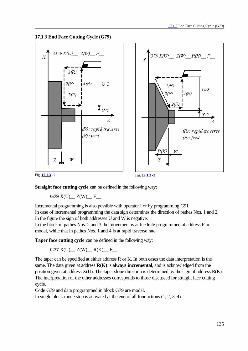
17.1.3 End Face Cutting Cycle (G79)
135
Fig. 17.1.3 -1 Fig. 17.1.3 -2
17.1.3 End Face Cutting Cycle (G79)
Straight face cutting cycle can be defined in the following way:
G79 X(U)__ Z(W)__ F__
Incremental programming is also possible with operator I or by programming G91.In case of incremental programming the data sign determines the direction of pathes Nos. 1 and 2.In the figure the sign of both addresses U and W is negative.In the block in pathes Nos. 2 and 3 the movement is at feedrate programmed at address F ormodal, while that in pathes Nos. 1 and 4 is at rapid traverse rate.
Taper face cutting cycle can be defined in the following way:
G77 X(U)__ Z(W)__ R(K)__ F__
The taper can be specified at either address R or K. In both cases the data interpretation is thesame. The data given at address R(K) is always incremental, and is acknowledged from theposition given at address X(U). The taper slope direction is determined by the sign of address R(K).The interpretation of the other addresses corresponds to those discussed for straight face cuttingcycle.Code G79 and data programmed in block G79 are modal.In single block mode stop is activated at the end of all four actions (1, 2, 3, 4).

17.1.3 End Face Cutting Cycle (G79)
136
Fig. 17.1.4 -3
In case of incremental programming the signs of addresses U, W and R(K) influence the movementdirections as follows:

17.1.4 Simple Cycle Application
137
Fig. 17.1.4 -1
17.1.4 Single Cycle Application
Both G codes and input parameters of cycles are modal. This means that if the cycle variables X(U),Z(W) or R(I or K), are already given and their values have not changed, they must not be rewrittenin pogram.. For example:
G91...G77 X–20 Z–50 F0.5
X–30X–40X–50...
In the above example only the value of depth ofcut (X) changes, therefore only this addressmust be refilled, the other values remainunchanged.The cycle is executed in the switched-on stateof the cycle provided a variable of X(U), Z(W)or R(I or K) referring to movement is also filled in. If for example in cycle state, function is executedin a separate block, the cycle state remains switched-on but the cycle is not repeated:
...G77 U–20 W–50 F0.5 (switch on and execute cycle)T202 (cycle switched on but not executed)U–30 (cycle executed)...
The cycle and the modal variables are deleted by interpolation G codes belonging to group No. 1 aswell as by all single-shot G codes except for dwell G4.
M, S, T function can also be written in blocks containing simple cycles. The functions are alwaysexecuted in action No. 1 of the cycle either parallel to movement or at the end of it. If in certaincases this may cause an inconvenience, the function shall be written in a separate block.

17.2.1 Stock Removal in Turning (G71)
138
Fig. 17.2.1 -1
17.2 Multiple Repetitive Cycles
Multiple repetitive cycles simplify the writing of machining programs. For example the profile of thepart must be specified for finishing. At the same time this profile determines the basis of cyclesexecuting stock removal (G71, G72, G73). Other than the stock removal also a finishing cycle(G70), a thread cutting cycle (G76) and two drilling cycles (G74, G75) are available.
17.2.1 Stock Removal in Turning (G71)
There are two kinds of stock removals in turning: Type 1 and 2.
Stock removal in turning type 1
If a finished shape of A)A’)B is given by the program as in the figure, the specified area is removedwith )d depth of cuts with finishing allowance )u/2 and )w left.
1st specification method:With command lines:
G71 U()d) R (e)G71 P (ns) Q (nf) U()u) W()w) F(f) S(s) T(t)
N(ns) X(U) ......
F___S___T___
N(nf) ...

17.2.1 Stock Removal in Turning (G71)
139
Fig. 17.2.1 -2
where:
)d: Depth of cut. Positive number interpreted always in radius . The depth of cut can also begiven at parameter 1339 DPTHCUT as well as this parameter is overwritten as the effect ofthe program command. This also means that in case the depth of cut is not specified thecontrol refers to this parameter.
e: Escaping amount. Positive number interpreted always in radius . The escaping amount canalso be given at parameter 1340 ESCAPE as well as this parameter is overwritten as theeffect of the program command. This also means that in case the escaping amount is notspecified the control refers to this parameter.
ns: Sequence number of the first block for the program of finishing shape (phase A)A’)B).
nf: Sequence number of the last block for the program of finishing shape (phase A)A’)B).
)u: Distance and direction of finishing allowance along X axis. Signed number interpreted indiameter or radius in function of X coordinate.
)w: Distance and direction of finishing allowance along Z axis. Signed number.
f, s, t: Any F, S or T function programmed in blocks ns to nf in the program for finishing shape(phase A)A’)B) is ignored and values f, s, t in block G71 are effective during the cycle.
The meaning of the value specified at address U being )d or )u depends on wether P and Q wereprogrammed in the given block. If not the meaning of address U is )d, if yes it is )u.The stock removal is executed by the block in which P and Q had been specified.The movement between points A)A’ must be specified in block No. ns given at address Pobligatorily by programming G00 or G01. The code defined here decides if the cutting in(movement in direction A)A’) is done at rapid traverse rate (in case programming G00) or atfeedrate (in case programming G01) in the course of stock removal. In this block no movement indirection P(ns) Z shall be given.Phase A’)B is the profile made up ofstraight lines and arcs. The profile mustbe monotonic increasing or decreasingboth in X and Z directions which meansthat regression is not possible in eitherway. The cycle can be used in all fourquadrants. The figure also shows the signof finishing allowance.F, S, T functions programmed in blocksns to nf are omitted and thoseprogrammed in block G71 (f, s, t) orpreviously are effective. The same is truefor constant surface speed programmedin blocks ns to nf, i.e., state G96 or G97and value of surface speed precedingblock G71 is effective.Blocks ns to nf cannot contain subprogram calls.

17.2.1 Stock Removal in Turning (G71)
140
Tool nose radius compensation calculation (G41, G42) can be switched on during cycle executionwith the obligation that it must be switched on (G41 or G42) and off (G40) between blocks rangingfrom ns to nf:
CORRECTN(ns) X(U) G41 ...
(G41)... ...
(G40)N(nf) G40 ...
or G41N(ns) X(U) ...
... ...
N(nf) ... G40
INCORRECT G41N(ns) X(U) ... ... ... G40N(nf) ...
orN(ns) G41 X(U) ...
... ...
N(nf) ... G40
If the cycle is interrupted during execution, edit mode is opened and parameter 1339 DPTHCUT isoverwritten, than in automatic mode the program is run by means of START the next cut is alreadytaken into account with the new depth of cut. The same goes for parameter 1340 ESCAPE i.e., forescaping amount.
2nd specification method:
G71 P (ns) Q (nf) U()u) W()w) D()d) F(f) S(s) T(t)N(ns) X(U) ......
F___S___T___
N(nf) ...Input parameters of the second specification method correspond to that of the first one.
Stock removal in turning type 2
Stock removal in turning type 2 must be defined like type 1, its code is G71 and its input parametersare also the same as those of type 1. The difference is the specification of the start up block of thefinishing shape (block No. ns). While in case of calling type 1 address Z cannot be referred to in thisblock, i.e., the movement of phase A)A’ must be perpendicular to Z axis, in case of calling type 2address Z must be obligatorily referred to in this block. In other words phase A)A’ must not beperpendicular to Z axis.

17.2.1 Stock Removal in Turning (G71)
141
Fig. 17.2.1 -3
Fig. 17.2.1 -4
Fig. 17.2.1 -5
Specification of type 1G71 U8 R1G71 P100 Q200 U0.5 W0.2 N100 X(U)___.........N200
Specification of type 2G71 U8 R1G71 P100 Q200 U0.5 W0.2 N100 X(U)___ Z(W)__.........N200
In case type 2 must be used with movement only in X direction, i.e., perpendicular to Z axis in thefirst block of finishing shape, incremental movement 0, i.e. ZI0 or W0 must be programmed along Zaxis.Stock removal in turning type 2 differs from type 1 in the profile not necessary being monotonicincreasing or decreasing in X direction, i.e., the profile may have concaves. The cycle can handle atmost 10 reflex pockets.
On the other hand in Z directionthe profile must remainmonotonic, it cannot includereflex.
The first block of the finishing shape (ns) may also containZ-direction movement (moreover address Z must be

17.2.1 Stock Removal in Turning (G71)
142
obligatorily referred to), i.e., the first cut must not be perpendicular to Z axis.

17.2.1 Stock Removal in Turning (G71)
143
Fig. 17.2.1 -6
Fig. 17.2.1 -7
In case of stock removal in turning type 2 theescaping amount is perpendicular to axis Z and isdone with valid escape amount “e”.
The below figure shows an example how does the cycle cut the rough workpiece.
In the above case Z-direction finishing allowance ()w) cannot be programmed (it must be W0),otherwise the tool may cut in a side wall.

17.2.2 Stock Removal in Facing (G72)
144
Fig. 17.2.2 -1
17.2.2 Stock Removal in Facing (G72)
There are two kinds of stock removals in facing: Type 1 and 2.
Stock removal in facing type 1
The stock removal in facing (G72) seen in the below figure is the same as stock removal in turningG71 except for that cutting is made by an operation parallel to X axis.
1st specification method:G72 W()d) R (e)G72 P (ns) Q (nf) U()u) W()w) F(f) S(s) T(t)
N(ns) Z(W) ......
F___S___T___
N(nf) ...The meaning of input parameters thoroughly correspond to those discussed for cycle G71.

17.2.2 Stock Removal in Facing (G72)
145
Fig. 17.2.2 -2
2nd specification method:G72 P (ns) Q (nf) U()u) W()w) D()d) F(f) S(s) T(t)
N(ns) Z(W) ......
F___S___T___
N(nf) ...
The cycle can be used in all four quadrants.The figure shows the finishing allowance signfor all four cases.In block No. ns describing movement betweenpoints A)A’ reference to X axis is notpossible, the movement must always be parallelto Z axis. The interpolation code (G00 or G01)defined in block No. ns determines if the cut inis done at feedrate or rapid traverse rate.The programmed profile must be monotonic,i.e., continuously increasing or decreasing alongboth axes.For tool radius compensation see cycle G71.
Stock removal in facing type 2
Stock removal in facing type 2 must be defined like type 1, its code is G72 and its input parametersare also the same as those of type 1. The difference is the specification of the start- up block of thefinishing shape (block No. ns). While in case of calling type 1 address X cannot be referred to inthis block, i.e., the movement of phase A)A’ must be perpendicular to X axis, in case of callingtype 2 address X must be obligatorily referred to in this block. In other words phase A)A’ must notbe perpendicular to X axis. Further on the same obligations are valid for the cycle as for G71 type2. The profile can also be reflex, however it must be monotonic in X direction.

17.2.3 Pattern Repeating Cycle (G73)
146
Fig. 17.2.3 -1
17.2.3 Pattern Repeating Cycle (G73)
This cycle can be used for cutting parts whose rough shape has already been made by roughmachining, forging or casting method. This function permits cutting a fixed pattern repeatedly, with apattern being displaced bit by bit.
1st specification method:Command
G73 U()i) W()k) R (d)G73 P (ns) Q (nf) U()u) W()w) F(f) S(s) T(t)
N(ns) ......
F___S___T___
N(nf) ...where:
)i: Distance and direction of relief along X axis. Signed number always interpreted in radius .The relief can also be given at parameter 1341 RELIEFX as well as this parameter isoverwritten as the effect of program command.

17.2.3 Pattern Repeating Cycle (G73)
147
)k: Distance and direction of relief along Z axis. Signed number always interpreted in radius .The relief can also be given at parameter 1342 RELIEFZ as well as this parameter isoverwritten as the effect of program command
d: Number of division. The number of division can also be given at parameter 1343 NUMDIVas well as this parameter is overwritten as the effect of program command. The valuespecified for relief (parameters RELIEFX, RELIEFZ) is divided by this number and theadvances are taken with the result in the course of stock removal.
ns: Sequence number of the fist block for the program of finishing shape (phase A)A’)B).
nf: Sequence number of the last block for the program of finishing shape (phase A)A’)B).
)u: Distance and direction of finishing allowance along X axis. Signed number interpretated indiameter or radius in function of X coordinate.
)w: Distance and direction of finishing allowance along Z axis. Signed number.
The meaning of addresses U and W defined in block G73 being )i and )k or )u and )w dependson if P and Q have been programmed in the given block. That is if P and Q have been programmed,then the meaning of U and W is )u and )w, if not, then it is )i and )k.The cycle is executed in the block containing P and Q. Blocks from ns to nf must contain thepositioning (phase A)A’) as well as the description of the finishing shape (phase A’)B). The cyclecan be executed in all four quadrants in function of the sign of values )i, )k, )u, )w. At the end ofcycle the tool returns to point “A”. The machining is continued from the following block.F, S, T functions programmed in blocks ns to nf are omitted and those programmed in block G71 (f,s, t) or previously are effective. The same is true for constant surface speed programmed in blocksns to nf,, i.e. state G96 or G97 and constant surface speed value preceding block G71 is effective.Blocks ranging from ns to nf cannot contain subprogram call.Tool nose radius compensation specification is possible in blocks defining the finishing shape with therestrictions discussed in description G71.
2nd specification method:
G73 P (ns) Q (nf) U()u) W()w) I()i) K()k) D(d) F(f) S(s) T(t)N(ns) ......
F___S___T___
N(nf) ...Input parameters of the second specification method correspond to those of the first one.

17.2.4 Finishing Cycle (G70)
148
Fig. 17.2.4-1
17.2.4 Finishing Cycle (G70)
After the stock removal with G71, G72 or G73 finishing can be defined by means of command G70.Finishing can be given with the following command:
G70 P (ns) Q (nf) U()u) W()w)
ns: Sequence number of the first block for the program of finishing shape.
nf: Sequence number of the last block for the program of finishing shape.
)u: Distance and direction of finishing allowance along X axis.. Signed number interpreted indiameter or radius in function of X coordinate.
)w: Distance and direction of finishing allowance along Z axis. Signed number.
F, S, T functions programmed in the program part between blocks ns and nf are executed duringthe cycle contrary to cycles G71, G72, G73.At the end of finishing cycle the tool returns to start point and the following block is loaded.Tool radius compensation calculation works in the course of finishing cycle.Finishing allowance can be defined at addresses U and W in case the finishing allowance is to beremoved in more steps.Blocks ranging from ns to nf cannot contain subprogram call.

17.2.5 End Face Peck Drilling Cycle (G74)
149
Fig. 17.2.5 -1
17.2.5 End Face Peck Drilling Cycle (G74)
The enclosed figure shows the process of end face peck drilling cycle G74. The drilling is in Zdirection.
1st specification method:
Command lineG74 R (e)G74 X(U) Z(W) P ()i) Q ()k) R ()d) F
where:
e: Return amountModal value, unchanging until overwritten. The return amount can also be given atparameter 1344 RETG74G75, as well as this parameter is overwritten as the effect ofprogram command.
X: X component of point B
U: Incremental amount from A to B
Z: Z component of point C
W: Incremental amount from A to C
)i: Movement amount in X direction. The number is positive and always interpreted in radius.
)k: Depth of cut in Z direction. The number is always positive
)d: Relief amount at the cutting bottom. The sign of )d is always positive (the movementdirection is always contrary to vector sign AB).

17.2.5 End Face Peck Drilling Cycle (G74)
150
However, if the filling out of addresses X(U) and P()i) is omitted the sign of R()d) isinterpreted and the movement direction is determined by the sign of )d at the cuttingbottom.
F: Feedrate
In the figure (F) indicates the phases done at feedrate and (R) indicates those done at rapid traverserate.The filling out of address R in block G74 determining e or )d depends upon the filling out ofaddress Z(W). If address Z(W) is filled out the interpretation of address R is )d.If the filling out of both addresses X(U) and P()i) is omitted movement occurs only along Z axis, i.e.drilling cycle takes place.
2nd specification method:
G74 X(U) Z(W) I ()i) K ()k) D ()d) F
The input parameters of the second specification method correspond to those of the first one.

17.2.6 Outer Diameter/Internal Diameter Drilling Cycle (G75)
151
Fig. 17.2.6 -1
17.2.6 Outer Diameter/Internal Diameter Drilling Cycle (G75)
The enclosed figure shows the process of outer diameter/internal diameter drilling cycle G75.
1st specification method:
G75 R (e)G75 X(U) Z(W) P ()i) Q ()k) R ()d) F
The interpretation of cycle variables corresponds to that of cycle G74 with the difference that thedrilling is in X direction, therefore the interpretation of addresses X(U) and Z(W) is reversed.
2nd specification method:
G75 X(U) Z(W) I ()i) K ()k) D ()d) F

17.2.7 Multiple Thread Cutting Cycle (G76)
152
Fig. 17.2.7 -1
Fig. 17.2.7 -2
17.2.7 Multiple Thread Cutting Cycle (G76)
The enclosed figure shows the process of multiple thread cutting cycle G76.

17.2.7 Multiple Thread Cutting Cycle (G76)
153
1st specification method:
Command linesG76 P (n) (r) (") Q ()dmin) R (d)G76 X(U) Z(W) P (k) Q ()d) R (i) F(E)(L)
where:n: Repetitive count in finishing (n=01...99)
The value is modal, unchanging until overwritten. The repetitive count of finishing can also begiven at parameter 1335 COUNTFIN as well as this parameter is overwritten as the effectof program command.
r: Chamfering amount (r=01...99)the tool is escaped in 45°during run out from thread. The chamfering amount can be givenwith the help of r. The phase length is
r@L/10where: L: The programmed thread lead. This value is modal, unchanging until overwritten. The chamfering amount can also be givenat parameter 1334 THRDCHMFR as well as this parameter is overwritten as the effect ofprogram command.
": Angle of tool tip in degree ("=01...99)This value is modal, unchanging until overwritten. The angle of tool tip can also be given atparameter 1336 TIPANGL as well as this parameter is overwritten as the effect of programcommand.
Values n, r and " can be specified altogether at address P. As all values are figured with two-digitnumbers, a six-digit number must be written at address P. For example if the number of finishingcycles is n=2, the chamfering amount is 1.5L (r=15) and a tool having a tip of 60° is applied, thenvalue P: P021560.
)dmin: Minimum cutting depth (positive number interpreted always in radius)If in course of thread cutting in cycle No. n the cutting depth is dn – dn–1< )dmin, then thecutting depth is always clamped to value )dmin. This value is modal, unchanging untiloverwritten. The minimum cutting depth value can also be given at parameter 1337MINTHRDP as well as this parameter is overwritten as the effect of program command.
d: Finishing allowance (positive number interpreted always in radius)Ths value is modal, unchanging until overwritten. The finishing allowance value can also begiven at parameter 1338 FINALLW as well as this parameter is overwritten as the effect ofprogram command.
The above listed parameters are the data of first block G76 P (n) (r) (") Q ()dmin) R (d). Thecontrol executes the receiving of the above parameters as the effect of code G76 provided neitheraddress X(U) nor Z(W) is filled out in block G76.
i: Taper size (interpreted always in radius)If i=0 or address R is not filled out ordinary linear thread cutting can be made.
k: Height of thread (positive number interpreted always in radius)

17.2.7 Multiple Thread Cutting Cycle (G76)
154
)d: Depth of cut in 1st cut (positive number interpreted always in radius)
L: Lead of threadIts programming corresponds to that of G33. Value written at address F indicates threadlead, while the value written at address E indicates the ridges pro inch.
The above parameters are the input data of second block G76 X(U) Z(W) R (i) P (k) Q ()d) F(E)(L). Thread cutting is only executed as the effect of the above block, which means that one ofaddresses X(U), Z(W) must be filled out. If neither coordinate is filled out the block is interpreted asparameter setting block.In the course of cycle execution the cut in, that is the movement between points A and C is done atrapid traverse rate, provided code G00 is in effect during cycle, while it is done at modal feed,provided code G01 is in effect during cycle.Feed movement is executed between points C and D in accordance with thread lead L specified ataddress F(E). All other phases are executed at rapid traverse rate.The thread is always cut on one side on the basis of relation for the nth path with thecutting amount per cycle always held constant..Chamfering is always done at the end of thread in compliance with the parameters set.
X(U), Z(W) the sign of these addresses defines the direction of cut in and thread cutting R(i) the sign of this address defines the taper slope direction.
As the effect of STOP the tool is escaped in accordance with the programmed chamfering asdiscussed in case of code G78 than the start point (A) is positioned. With START button pressedthe interrupted cut is started from the beginning.
2nd specification method:
G76 X(U) Z(W) I(i) K(k) D()d) A(") F(E)(L) Q P
Interpretation of data i, k, )d, L corresponds to those discussed for the 1st method. Similarly to the 1st method the angle of tool tip can be defined at address “A” ("). The difference isin the unit specifiable being 1° for the 1st method, while 0.001° for the 2nd one. In case address “A”is not filled out value " is taken from parameter. However the specification of address “A” does notchange the value of parameter 1336 TIPANGL.Input parameters n, r, ", )dmin and d are acknowledged by the control in case of the 2nd threadspecification method just as in case of the 1st. one. Likewise input parameters can be given withprevious block G76 P (n) (r) (") Q ()dmin) R (d).The control refers to block specification made according to the 2nd method if address K is filled outin block.
Q: Angle value of thread start calculated from encoder zero pulse in °. Interpretation of theaddress corresponds to that of G33.
P: Thread cutting method.Five thread cutting methods can be selected on the basis of the below figuresP1: Cutting amount constant, single edge cuttingP2: Both edge cuttingP3: Cutting depth constant, single edge cutting

17.2.7 Multiple Thread Cutting Cycle (G76)
155
Fig. 17.2.7 -3
Fig. 17.2.7 -4
P4: Cutting depth constant, both edge cuttingP5: Cutting amount constant, both edge cutting

17.2.7 Multiple Thread Cutting Cycle (G76)
156
Fig. 17.2.7 -6
Fig. 17.2.7 -5

17.2.7 Multiple Thread Cutting Cycle (G76)
157
Fig. 17.2.7 -7
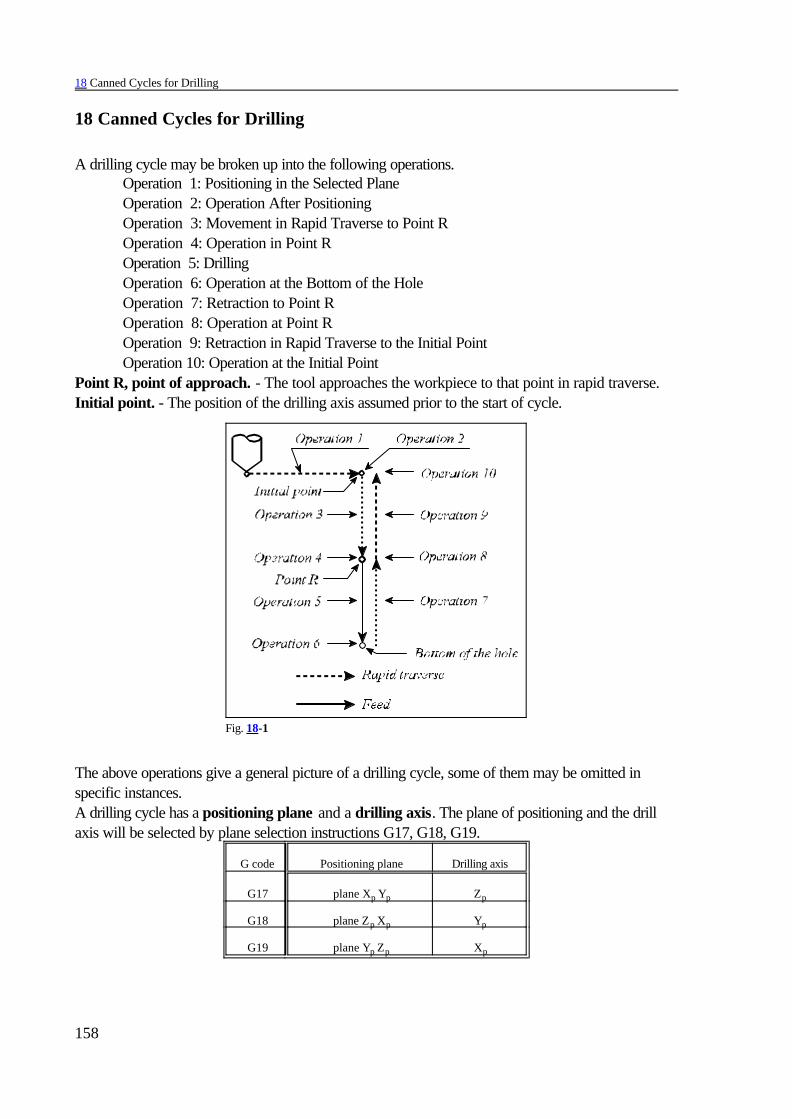
18 Canned Cycles for Drilling
158
Fig. 18-1
18 Canned Cycles for Drilling
A drilling cycle may be broken up into the following operations.Operation 1: Positioning in the Selected PlaneOperation 2: Operation After PositioningOperation 3: Movement in Rapid Traverse to Point ROperation 4: Operation in Point ROperation 5: DrillingOperation 6: Operation at the Bottom of the HoleOperation 7: Retraction to Point ROperation 8: Operation at Point ROperation 9: Retraction in Rapid Traverse to the Initial PointOperation 10: Operation at the Initial Point
Point R, point of approach. - The tool approaches the workpiece to that point in rapid traverse.Initial point. - The position of the drilling axis assumed prior to the start of cycle.
The above operations give a general picture of a drilling cycle, some of them may be omitted inspecific instances.A drilling cycle has a positioning plane and a drilling axis. The plane of positioning and the drillaxis will be selected by plane selection instructions G17, G18, G19.
G code Positioning plane Drilling axis
G17 plane Xp Yp Zp
G18 plane Zp Xp Yp
G19 plane Yp Zp Xp
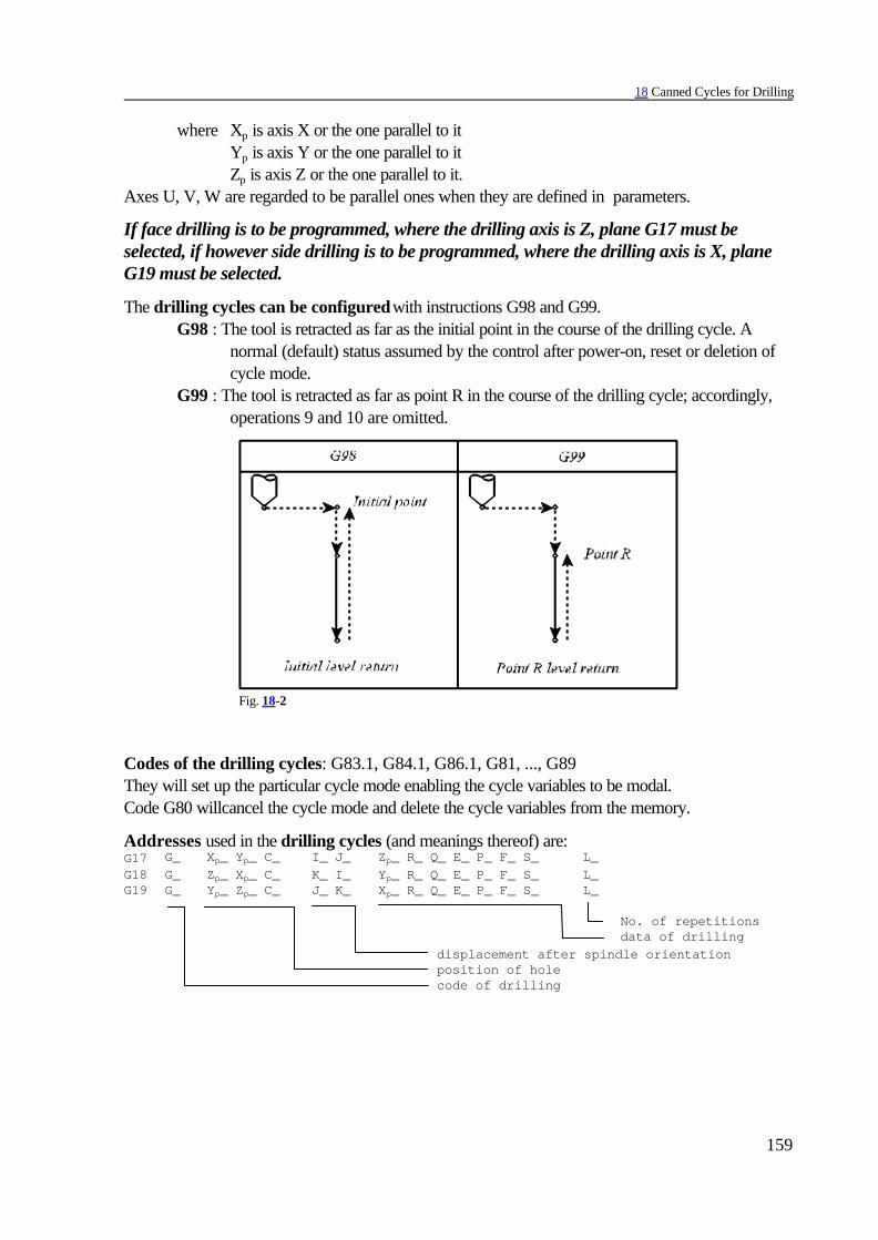
18 Canned Cycles for Drilling
159
Fig. 18-2
where Xp is axis X or the one parallel to itYp is axis Y or the one parallel to itZp is axis Z or the one parallel to it.
Axes U, V, W are regarded to be parallel ones when they are defined in parameters.
If face drilling is to be programmed, where the drilling axis is Z, plane G17 must beselected, if however side drilling is to be programmed, where the drilling axis is X, planeG19 must be selected.
The drilling cycles can be configured with instructions G98 and G99.G98 : The tool is retracted as far as the initial point in the course of the drilling cycle. A
normal (default) status assumed by the control after power-on, reset or deletion ofcycle mode.
G99 : The tool is retracted as far as point R in the course of the drilling cycle; accordingly,operations 9 and 10 are omitted.
Codes of the drilling cycles: G83.1, G84.1, G86.1, G81, ..., G89They will set up the particular cycle mode enabling the cycle variables to be modal.Code G80 willcancel the cycle mode and delete the cycle variables from the memory.
Addresses used in the drilling cycles (and meanings thereof) are:G17 G_ Xp_ Yp_ C_ I_ J_ Zp_ R_ Q_ E_ P_ F_ S_ L_G18 G_ Zp_ Xp_ C_ K_ I_ Yp_ R_ Q_ E_ P_ F_ S_ L_G19 G_ Yp_ Zp_ C_ J_ K_ Xp_ R_ Q_ E_ P_ F_ S_ L_
No. of repetitionsdata of drilling
displacement after spindle orientationposition of holecode of drilling

18 Canned Cycles for Drilling
160
Fig. 18-3
The code of drilling:
For meanings of the codes see below.Each code will be modal until an instruction G80 or a code is programmed, that belongs to G codegroup 1 (interpolation codes: G01, G02, G03, G33).As long as the cycle state is on (instructions G83.1, G84.1, G86.1, G81,...G89), the modal cyclevariables will be modal between drilling cycles of various types, too.
Initial point:
The initial point is the position of axis selected for drilling; it will be recorded – when the cycle mode is set up. For example, in the case of
N1 G17 G90 G0 Z200N2 G81 X0 C0 Z50 R150N3 X100 C30 Z80
the position of initial point will be Z=200 in blocks N2 and N3, too. – Or when a new drilling axis is selected. For example:
N1 G17 G90 G0 Z200 W50N2 G81 X0 C0 Z50 R150N3 X100 C30 W20 R25
position of start point is Z=200 in block N2position of start point is W=50 in block N3
Programming of R is mandatory when the selection of drilling axis is changed, or else error message3053 NO BOTTOM OR R POINT is returned.
Position of hole - Xp, Yp, Zp, C
Of the coordinate values entered, those in the selected plane will be taken for the position of thehole.The values entered may be incremental or absolute ones, rectangular (Cartesian) or polarcoordinates in metric or inch units.The mirror image, coordinate systemrotation and scaling commands areapplicable to the coordinate valuesentered.The control moves to the position of holein rapid traverse regardless of which codein group1 is in effect.
Displacement after spindleorientation - I, J, K
If the particular machine is provided withthe facility of spindle orientation, the toolcan be retracted off the surface in fineboring and back boring cycles G76 andG87 in order not to scratch the surface ofthe hole. Now the direction in which the
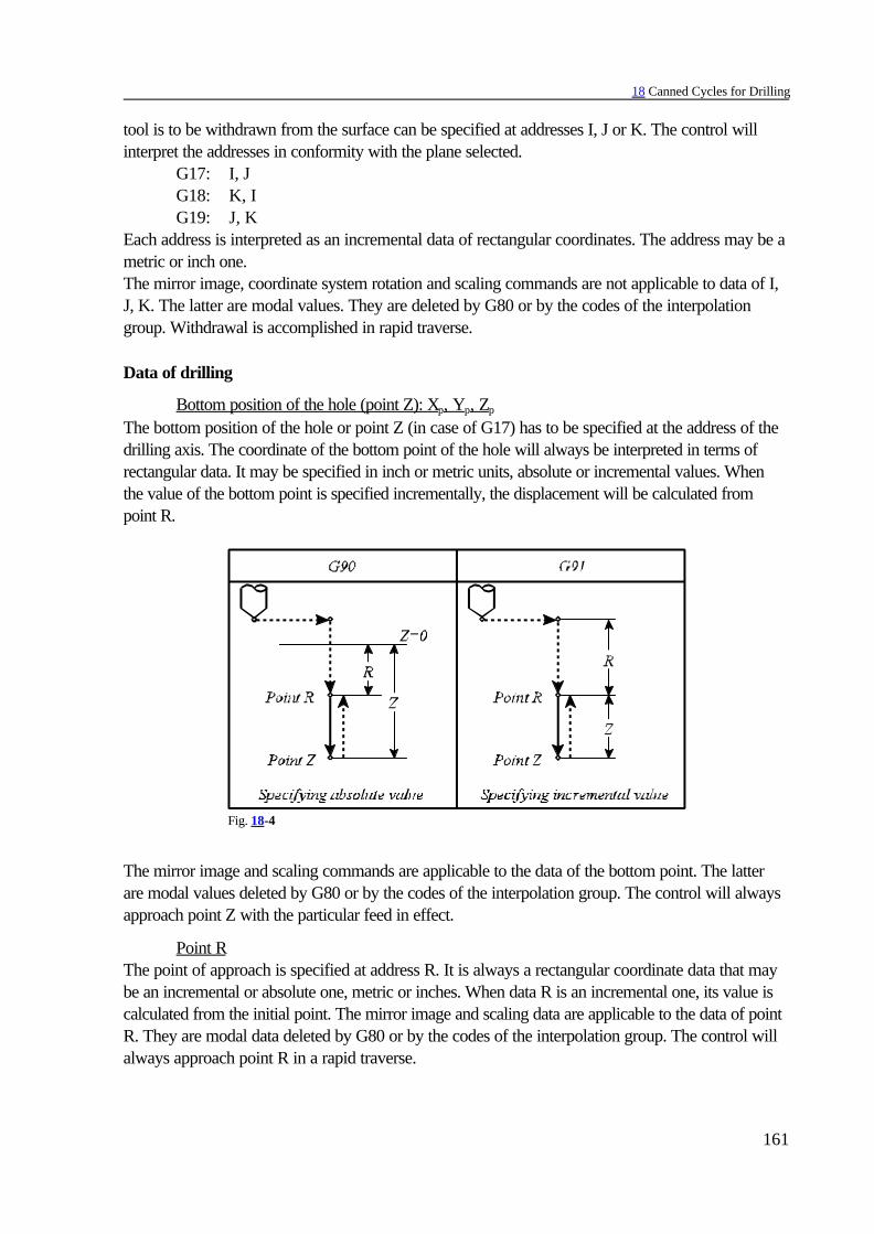
18 Canned Cycles for Drilling
161
Fig. 18-4
tool is to be withdrawn from the surface can be specified at addresses I, J or K. The control willinterpret the addresses in conformity with the plane selected.
G17: I, JG18: K, IG19: J, K
Each address is interpreted as an incremental data of rectangular coordinates. The address may be ametric or inch one.The mirror image, coordinate system rotation and scaling commands are not applicable to data of I,J, K. The latter are modal values. They are deleted by G80 or by the codes of the interpolationgroup. Withdrawal is accomplished in rapid traverse.
Data of drilling
Bottom position of the hole (point Z): Xp, Yp, Zp
The bottom position of the hole or point Z (in case of G17) has to be specified at the address of thedrilling axis. The coordinate of the bottom point of the hole will always be interpreted in terms ofrectangular data. It may be specified in inch or metric units, absolute or incremental values. Whenthe value of the bottom point is specified incrementally, the displacement will be calculated frompoint R.
The mirror image and scaling commands are applicable to the data of the bottom point. The latterare modal values deleted by G80 or by the codes of the interpolation group. The control will alwaysapproach point Z with the particular feed in effect.
Point RThe point of approach is specified at address R. It is always a rectangular coordinate data that maybe an incremental or absolute one, metric or inches. When data R is an incremental one, its value iscalculated from the initial point. The mirror image and scaling data are applicable to the data of pointR. They are modal data deleted by G80 or by the codes of the interpolation group. The control willalways approach point R in a rapid traverse.

18 Canned Cycles for Drilling
162
Cut-in value (Q)It is the depth of the cut-in, in the cycles of G73 and G83. It is invariably an incremental, rectangularpositive data (a modal one). Its value will be deleted by G80 or by the codes of the interpolationgroup. The scaling does not affect the value of cut-in depth.
Auxiliary data (E)The extent of retraction in the cycle of G73 and value of clearance in the cycle of G83 is specifiedon address E. It is always an incremental, rectangular, positive data. The scaling command has noeffect to the auxiliary data. (Modal value). Its value will be deleted by G80 or by the codes of theinterpolation group. Unless it has been programmed, the control will take the necessary value fromparameter RETG73, or CLEG83.
Dwell (P)Specifies the time of dwell at the bottom of the hole. Its specification is governed by the rulesdescribed at G04. The value of the dwell is a modal one deleted by G80 or by the codes of theinterpolation group.
Feed (F)It will define the feed. A modal value, re-written only by the programming of another data F. It willnot be deleted by G80 or some other code.
Spindle speed (S)A modal value re-written only by programming another data S. It will not be deleted by G80 orsome other code.
Number of repetitions (L)Defining the number of cycle repetitions over the range of 1 through 9999. Unless L is filled in, thevalue of L=1 is assumed. In the case of L=0 the data of the cycle will be stored but not executed.The value of L is effective only in the block in which it has been specified.
Examples of modal drilling codes and cycle variables:
N1 G17 G0 Z_ M3N2 G81 X_ C_ Z_ R_ F_
It is mandatory to specify the data of drilling (Z, R) at the beginning of cycle mode.N3 X_
Since the data of drilling have been specified in block N2 and they are used unchanged in N3, theyneed not be filled in again, i.e., G81, Z_, R_, F_ may be omitted. The position of the hole is variedin direction X only, the tool moves in that direction and will drill the same hole as in block N2.
N4 G82 C_ Z_ P_
The position of the hole is shifted in direction C. The method of drilling complies with G82, thebottom point assumes a new value (Z), the point R and the feed (R, F) are taken from block N2.
N5 G80 M5
The cycle mode and the modal cycle variables (except for F) will be deleted.N6 G85 C_ Z_ R_ P_ M3
Since the data of drilling are deleted in block N5 under the command of G80, the values of Z, Rand P have to be specified again.
N7 G0 X_ C_
The cycle mode and the modal cycle variables (except for F) will be deleted.

18 Canned Cycles for Drilling
163
Fig. 18-5
Fig. 18-6
Examples of using cycle repetitions :If a particular type of hole is to be drilled with unchanged parameters at equally spaced positions,the number of repetitions can be specified at address L. The value of L is only effective in the block,in which it has been specified.
N1 G90 G19 G0 X300 Z40 C0 M3N2 G91 G81 X–40 Z100 R–20 F50 L5
Under the above instructions the control will drill 5identical holes spaced at 100mm along axis Z. Theposition of the first hole is Z=140, C=0. Since thisis a side drilling with X axis, plane G19 has beenselected.
Under G91 the position of the hole has been specified incrementally.N1 G90 G17 G0 X200 C–60 Z50 N2 G81 CI60 Z–40 R3 F50 L6
Under the above commands the control will drill 6holes spaced at 60 degrees around a 100mm-radius circle. The position of the first hole coincideswith the point of X=200 C=0 coordinates. Since itis face drilling (the drill axis is Z) plane G17 isspecified.

18 Canned Cycles for Drilling
164
Fig. 18.1.1-1
18.1 Detailed Description of Canned Cycles
18.1.1 High Speed Peck Drilling Cycle (G83.1)
The variables used in the cycle areG17 G83.1 Xp__ Yp__ C__ Zp__ R__ Q__ E__ F__ L__G18 G83.1 Zp__ Xp__ C__ Yp__ R__ Q__ E__ F__ L__G19 G83.1 Yp__ Zp__ C__ Xp__ R__ Q__ E__ F__ L__
The operations of the cycle are1. rapid-traverse positioning2. -3. rapid-traverse movement to point R4. -5. drilling as far as the point Z, with feed F6. -7. with G99, retraction to point R, in rapid traverse8. -9. with G98, retraction to the initial point, in rapid traverse
10. -Description of drilling operation 5 is as follows: – Drilling the cut-in depth specified at address Q in the workpiece, with feed, – rapid-traverse retraction by the distance specified at address E or in parameter RETG73, – drilling cut-in depth Q again, reckoned from the end point of the previous cut-in, – rapid-traverse retraction at the value specified at address E.The above procedure is carried on as far as the bottom point specified at address Z.

18 Canned Cycles for Drilling
165
Fig. 18.1.2-1
18.1.2 Counter Tapping Cycle (G84.1)
This cycle can be used only with a spring tap. The variables used in the cycle areG17 G84.1 Xp__ Yp__ C__ Zp__ R__ (P__) F__ L__G18 G84.1 Zp__ Xp__ C__ Yp__ R__ (P__) F__ L__G19 G84.1 Yp__ Zp__ C__ Xp__ R__ (P__) F__ L__
Prior to start the cycle, the spindle has to be started or programmed to rotate in the direction of M4(counter-clockwise).The value of feed has to be specified in conformity with the thread pitch of the tapper. – In state G94 (feed per minute):
where P is the thread pitch in mm/rev or inches/rev, S is the spindle speed in rpm
– In state G95 (feed per revolution):
where P is the thread pitch in mm/rev or inches/rev.The operations of the cycle:
1. rapid-traverse positioning in the selected plane2. -3. rapid-traverse movement as far as point R4. -5. drilling as far as thebottom point, with feed F (override and stop inhibited)6. dwell with the value specified at address P, provided parameter TAPDWELL is
enabled (=1) spindle direction reversal (M3)7. retraction as far as point R with feed F (override and stop inhibited)8. spindle direction reversal (M4)9. with G98, rapid-traverse retraction to the initial point
10. -

18 Canned Cycles for Drilling
166
Fig. 18.1.3-1
18.1.3 Fine Boring Cycle (G86.1)
Cycle G76 is only applicable when the facility of spindle orientation is incorporated in the machine-tool. In this case parameter ORIENT1 is to be set to 1, otherwise message 3052 ERROR IN G76 isreturned.Since, on the bottom point, the cycle performs spindle orientation and recesses the tool from thesurface with the values specified at I, J and K, the part will not be scratched when the tool iswithdrawn.The variables used in the cycle are
G17 G86.1 Xp__ Yp__ C__ I__ J__ Zp__ R__ P__ F__ L__G18 G86.1 Zp__ Xp__ C__ K__ I__ Yp__ R__ P__ F__ L__G19 G86.1 Yp__ Zp__ C__ J__ K__ Xp__ R__ P__ F__ L__
Command M3 has to be issued prior to starting the cycle.The operations of the cycle:
1. rapid-traverse positioning in the selected plane2. -3. rapid-traverse movement as far as point R4. -5. boring as far as the point Z, with feed F6. – dwell with the value specified at address P
– spindle orientation (M19)– rapid-traverse receding of the tool with values I, J, K in the selected plane
7. with G99, rapid-traverse retraction as far as point R8. with G99,
– rapid-traverse retraction of the tool in the selected plane, opposite to the valuesspecified at I, J, K
– spindle re-started in direction M39. with G98, rapid-traverse retraction to the initial point
10. with G98, – rapid-traverse retraction of the tool in the selected plane, opposite to the values
specified at I, J, K

18 Canned Cycles for Drilling
167
Fig. 18.1.5-1
– spindle re-started in direction M3
18.1.4 Canned Cycle for Drilling Cancel (G80)
The code G80 will cancel the cycle state, the cycle variables will be deleted.Z and R will assume incremental 0 value (the rest of variables will assume 0).With coordinates programmed in block G80 but no other instruction is issued, the movement will becarried out according to the interpolation code in effect prior to activation of the cycle (G codegroup 1).
18.1.5 Drilling, Spot Boring Cycle (G81)
The variables used in the cycle areG17 G81 Xp__ Yp__ C__ Zp__ R__ F__ L__G18 G81 Zp__ Xp__ C__ Yp__ R__ F__ L__G19 G81 Yp__ Zp__ C__ Xp__ R__ F__ L__
The operations of the cycle are1. rapid-traverse positioning in the selected plane2. -3. rapid-traverse movement as far as point R4. -5. drilling as far as the point Z, with feed F6. -7. with G99, retraction to point R, in rapid traverse8. -9. with G98, rapid-traverse retraction to the initial point
10. -

18 Canned Cycles for Drilling
168
Fig. 18.1.6-1
18.1.6 Drilling, Counter Boring Cycle (G82)
The variables used in the cycle areG17 G82 Xp__ Yp__ C__ Zp__ R__ P__ F__ L__G18 G82 Zp__ Xp__ C__ Yp__ R__ P__ F__ L__G19 G82 Yp__ Zp__ C__ Xp__ R__ P__ F__ L__
the operations of the cycle are1. rapid-traverse positioning in the selected plane2. -3. rapid-traverse movement as far as point R4. -5. drilling as far as the bottom point, with feed F6. dwell for the time specified at address P7. with G99, rapid-traverse retraction to point R8. -9. with G98, rapid-traverse retraction to the initial point
10. -

18 Canned Cycles for Drilling
169
Fig. 18.1.7-1
18.1.7 Peck Drilling Cycle (G83)
The variables used in the cycle areG17 G83 Xp__ Yp__ C__ Zp__ R__ Q__ E__ F__ L__G18 G83 Zp__ Xp__ C__ Yp__ R__ Q__ E__ F__ L__G19 G83 Yp__ Zp__ C__ Xp__ R__ Q__ E__ F__ L__
The oprations of the cycle are1. rapid-traverse positioning in the selected plane2. -3. rapid-traverse movement to point R4. -5. drilling to the bottom point, with feed F6. -7. with G99, rapid-traverse retraction to point R8. -9. with G98, rapid-traverse retraction to the initial point
10. -Description of drilling operation 5 is as follows: – Drilling the depth specified at address Q, with feed, – rapid-traverse retraction to point R, – rapid-traverse approach of the previous depth as far as the clearance amount specified on
address E, – drilling depth Q again, reckoned from the previous cut-in, with feed F (displacement E+Q), – rapid-traverse retraction to point R. The above procedure is carried on as far as the bottom point specified at address Z.

18 Canned Cycles for Drilling
170
Fig. 18.1.8-1
Distance E will be taken from the program (address E) or from parameter CLEG83.
18.1.8 Tapping Cycle (G84)
This cycle can be used only with a spring tap.The variables used in the cycle are
G17 G84 Xp__ Yp__ C__ Zp__ R__ (P__) F__ L__G18 G84 Zp__ Xp__ C__ Yp__ R__ (P__) F__ L__G19 G84 Yp__ Zp__ C__ Xp__ R__ (P__) F__ L__
Direction of spindle rotation M3 (clockwise) has to be selected prior to starting the cycle.The value of feed has to be specified in conformity with the thread pitch of the tap. – In state G94 (feed per minute):
where P is the thread pitch in mm/rev or inches/rev.S is the spindle speed in rpm
– In state G95 (feed per revolution):
where P is the thread pitch in mm/rev or inches/rev.
The operations of the cycle are1. rapid-traverse positioning in the selected plane2. -3. rapid-traverse movement to point R4. -5. tapping to the bottom point with feed F, override and stop inhibited6. – dwell with value specified at address P, provided parameter TAPDWELL is
enabled (=1),– reversal of spindle direction (M4)
7. retraction to point R with feed F, override and stop inhibited8. reversal of spindle direction (M3)
18 Canned Cycles for Drilling
171
9. with G98, rapid-traverse retraction to the initial point10. -
18.1.9 Rigid (Clockwise and Counter-clockwise) Tap Cycles (G84.2, G84.3)
In a tapping cycle the quotient of the drill-axis feed and the spindle rpm must be equal to the threadpitch of the tap. In other words, under ideal conditions of tapping, the quotient
must be constant from moment to moment
where P is the thread pitch (mm/rev or inches/rev), F is the feed (mm/minute or inches/minute), S is the rpm of spindle (revolutions/minute).
The spindle speed and the feed of the tapping axis are controlled completely independently in left-hand and right-hand tapping cycles G74 and G84, respectively. Accordingly, the above conditioncannot be fulfilled to full accuracy. This is particularly applicable to the bottom of the hole where thefeed of the drill axis and the spindle speed ought to be slowed down and stopped in synchronism,and accelerated so in the opposite direction. This condition cannot be fulfilled from a controlledpoint of view in the above case. The above problem can be eliminated by a spring tap, that would
compensate for the fluctuations in the value of quotient .
A different principle of control is adopted in drilling cycles G84.2 and G84.3 enabling rigid tap
(tapping without spring). There the control maintains quotient constant from moment to
moment.The control will regulate only the speed of the spindle in the former case, in the latter case itsposition is also controlled. The movements of the drilling axis and the spindle are linked through
linear interpolations in cycles G84.2 and G84.3. In this way quotient can be maintained
constant in the acceleration and deceleration stages as well.G84.2: Rigid tapping cycleG84.3: Rigid counter tapping cycle
The above cycles are only applicable with machines in which the spindle is fitted with an encoder,and the main drive can be fed back for position control (parameter INDEX1=1). Otherwise thecontrol will return error message 3052 ERROR IN G76, G87 when the mode is called.The variables used in the cycle are
G17 G84._ Xp__ Yp__ C__ Zp__ R__ F__ S__ L__G18 G84._ Zp__ Xp__ C__ Yp__ R__ F__ S__ L__G19 G84._ Yp__ Zp__ C__ Xp__ R__ F__ S__ L__
The spindle comes to a halt at the end of the cycle, if necessary, it has to be re-started by theprogrammer.The feed and the spindle rpm have to be specified in conformity with the thread pitch of the tap.

18 Canned Cycles for Drilling
172
Fig. 18.1.9-1
– In state G94 (feed per minute), where P is the thread pitch in mm/rev or inches/rev,
S is the spindle speed in rpmIn this case the displacement and the feed along the drilling axis and the spindle will be asfollows (Z assumed to be the drilling axis):
displacement feed
Z z= distance between point R and point Z
S
– In state G95 (feed per revolution), where P is the thread pitch in mm/rev or inches/rev. Evidently, the thread pitch can be
programmed directly in state G95 (feed per revolution), but S also has to beprogrammed in order to define the feed.
In this case, the displacement and the feed along the drilling axis and the spindle will be asfollows (assuming axis Z to be the drilling axis):
displacement feed
Zz=R distance between point and the base
point
S
In the case of G84.2, the operations of the cycle are1. rapid-traverse positioning in the selected plane2. -3. rapid-traverse movement to point R

18 Canned Cycles for Drilling
173
Fig. 18.1.9-2
4. spindle orientation (M19)5. linear interpolation between the drilling axis and the spindle, with the spindle
rotated in clockwise direction6. -7. linear interpolation between the drilling axis and the spindle, with the spindle
being rotated counter-clockwise8. -9. with G98, rapid-traverse retraction to the initial point
10. -
In the case of G84.3, the operations of the cycle are1. rapid-traverse positioning in the selected plane2. -3. rapid-traverse movement to point R4. spindle orientation (M19)5. linear interpolation between the drilling axis and the spindle, with the spindle
rotated in counter-clockwise direction (-)6.7. linear interpolation between the drilling axis and the spindle, with the spindle
being rotated clockwise (+)8. -9. with G98, rapid-traverse retraction to the initial point
10. -

18 Canned Cycles for Drilling
174
Fig. 18.1.10-1
18.1.10 Boring Cycle (G85)
The variables used in the cycle areG17 G85 Xp__ Yp__ C__ Zp__ R__ F__ L__G18 G85 Zp__ Xp__ C__ Yp__ R__ F__ L__G19 G85 Yp__ Zp__ C__ Xp__ R__ F__ L__
The operations of the cycle are1. rapid-traverse positioning in the selected plane2. -3. rapid-traverse movement to point R4. -5. boring as far as the bottom point with feed F6. -7. retraction to point R with feed F8. -9. with G98, rapid-traverse retraction to the initial point
10. -

18 Canned Cycles for Drilling
175
Fig. 18.1.11-1
18.1.11 Boring Cycle Tool Retraction with Rapid Traverse (G86)
The variables used in the cycle areG17 G86 Xp__ Yp__ C__ Zp__ R__ F__ L__G18 G86 Zp__ Xp__ C__ Yp__ R__ F__ L__G19 G86 Yp__ Zp__ C__ Xp__ R__ F__ L__
The spindle has to be given rotation of M3 when the cycle is started.The operations of the cycle are
1. rapid-traverse positioning in the selected plane2. -3. rapid-traverse movement to point R4. -5. boring as far as the point Z with feed F6. stopping the spindle (M5)7. with G99, rapid-traverse retraction to point R8. with G99, spindle re-started (M3)9. with G98, rapid-traverse retraction to the start point
10. with G98, spindle re-started (M3)

18 Canned Cycles for Drilling
176
Fig. 18.1.12-1
18.1.12 Boring Cycle/Back Boring Cycle (G87)
The cycle will be performed in two different ways.
A. Boring Cycle, Manual Operation at Bottom PointUnless the machine is provided with the facility of spindle orientation (parameter ORIENT1=0), thecontrol will act according alternative "A".The variables used in the cycle are
G17 G87 Xp__ Yp__ C__ Zp__ R__ F__ L__G18 G87 Zp__ Xp__ C__ Yp__ R__ F__ L__G19 G87 Yp__ Zp__ C__ Xp__ R__ F__ L__
The spindle must be started in M3 when the cycle is started.The operations of the cycle are
1. rapid-traverse positioning in the selected plane2. -3. rapid-traverse movement to point R4. -5. boring as far as the bottom point with feed F6. – spindle stop (M5)
– the control assumes STOP state (M0), from which the operator can get in one ofthe manual movement modes (JOG, INCREMENTAL JOG, or HANDLE)and operate the machine manually, for example retract the tool from the sideof the hole then remove the tool from the hole. After returning AUTO modemachining can be continued by START.
7. with G99, START followed by rapid-traverse retraction to point R8. with G99, spindle re-started (M3)9. with G98, START followed by rapid-traverse retraction to the initial point
10. with G98, spindle re-started (M3)
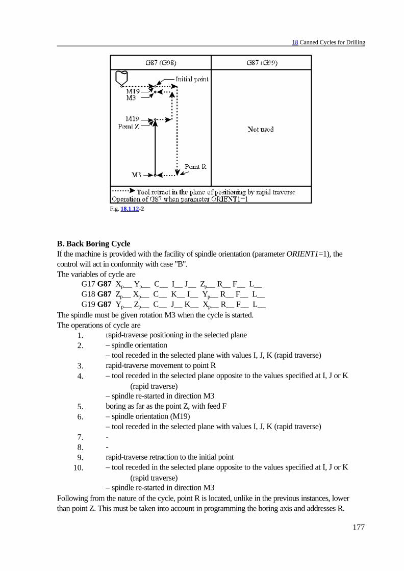
18 Canned Cycles for Drilling
177
Fig. 18.1.12-2
B. Back Boring CycleIf the machine is provided with the facility of spindle orientation (parameter ORIENT1=1), thecontrol will act in conformity with case "B".The variables of cycle are
G17 G87 Xp__ Yp__ C__ I__ J__ Zp__ R__ F__ L__G18 G87 Zp__ Xp__ C__ K__ I__ Yp__ R__ F__ L__G19 G87 Yp__ Zp__ C__ J__ K__ Xp__ R__ F__ L__
The spindle must be given rotation M3 when the cycle is started.The operations of cycle are
1. rapid-traverse positioning in the selected plane2. – spindle orientation
– tool receded in the selected plane with values I, J, K (rapid traverse)3. rapid-traverse movement to point R4. – tool receded in the selected plane opposite to the values specified at I, J or K
(rapid traverse)– spindle re-started in direction M3
5. boring as far as the point Z, with feed F6. – spindle orientation (M19)
– tool receded in the selected plane with values I, J, K (rapid traverse)7. -8. -9. rapid-traverse retraction to the initial point
10. – tool receded in the selected plane opposite to the values specified at I, J or K (rapid traverse)
– spindle re-started in direction M3Following from the nature of the cycle, point R is located, unlike in the previous instances, lowerthan point Z. This must be taken into account in programming the boring axis and addresses R.

18 Canned Cycles for Drilling
178
Fig. 18.1.13-1
18.1.13 Boring Cycle (Manual Operation on the Bottom Point) (G88)
The variables used in the cycle areG17 G88 Xp__ Yp__ C__ Zp__ R__ P__ F__ L__G18 G88 Zp__ Xp__ C__ Yp__ R__ P__ F__ L__G19 G88 Yp__ Zp__ C__ Xp__ R__ P__ F__ L__
The spindle must be given rotation M3 when the cycle is started.The operations of the cycle are
1. rapid-traverse positioning in the selected plane2. -3. rapid-traverse movement to point R4. -5. boring as far as the bottom point with feed F6. – dwell with value P
– spindle stop (M5)– the control assumes STOP state (M0), from which the operator can get in one of
the manual movement modes (JOG, INCREMENTAL JOG, or HANDLE)and operate the machine manually, for example retract the tool from the sideof the hole then remove the tool from the hole. After returning AUTO modemachining can be continued by START.
7. with G99, START followed by retraction to point R (rapid traverse)8. with G99, spindle re-started (M3)9. with G98, rapid-traverse retraction to the initial point
10. with G98, spindle re-started (M3) The cycle is the same as case "A" of G87 but dwelling before the spindle stop.

18 Canned Cycles for Drilling
179
Fig. 18.1.14-1
18.1.14 Boring Cycle (Dwell on the Bottom Point, Retraction with Feed) (G89)
The variables used in the cycle areG17 G89 Xp__ Yp__ Zp__ R__ P__ F__ L__G18 G89 Zp__ Xp__ Yp__ R__ P__ F__ L__G19 G89 Yp__ Zp__ Xp__ R__ P__ F__ L__
The operations of the cycle are1. rapid-traverse positioning in the selected plane2. -3. rapid-traverse movement to point R4. -5. boring as far as the bottom point, with feed F6. dwelling with the value specified at address P7. retraction to point R, with feed F8. -9. with G98, rapid-traverse retraction to the initial point
10. -Except for dwelling, the cycle is identical with G85.
18.2 Notes to the Use of Canned Cycles for Drilling
– The drilling cycle will be executed in cycle mode provided a block without code G contains oneof the addresses
Xp, Yp, Zp, C or ROtherwise, the drilling cycle will not be executed.
– With dwell G04 P programmed in cycle mode, the command will be executed in conformity withP programmed, but the cycle variable of dwell will not be deleted and will not be re-written.
– The values of I, J, K, Q, E, P have to be specified in a block, in which drilling is also performed,or else the values will not be stored.

18 Canned Cycles for Drilling
180
To illustrate the foregoing, let us see the following example. G81 X_ C_ Z_ R_ F (the drilling cycle is executed)
X (the drilling cycle is executed)F_ (the drilling cycle is not executed, F is
over-written)M_ (the drilling cycle is not executed, code M
is executed) G4 P_ (the drilling cycle is not executed, the
dwell will be re-written, but not the dwellvalue of cycle variable)
I_ Q_ (the drilling cycle is not executed, theprogrammed values will not be recorded ascycle variables)
– If a function as well as a drilling cycle are programmed in one block, the function will be executedat the end of the first operation, on completion of positioning. If L has also beenprogrammed in the cycle, the function will be executed in the first round only.
– In block-byQblock mode, the control will stop after each of operations 1, 3 and 10 during thecycle.
– The STOP button is ineffective to each of operations 5, 6 and 7 of cycles G84.1, G84. If STOPis depressed during those operations, the control will continue its functioning, and will notstop before the end of operation 7.
– The feed and the spindle override will always be 100% in each of operations 5, 6 and 7 of cyclesG74, G84 regardless of the override switch setting.
) If Tnnmm is programmed in cycle block the new length compensation is taken into account incase of both for positioning in the selected plane and for drilling.

19 Polygonal Turning
181
Fig. 19-1
Fig. 19.1-1
Fig. 19.1-2
19 Polygonal Turning
In case of polygonal turning both the tool and the workpiece arerotated in relation to each other by a specified revolution ratio.Polygons with varying side number are resulted from the change ofthe revolution ratio and the number of cutters of the rotating tool.The side number of the polygon is determined by the multiplicationof the revolution ratio and of the number of cutters. If for examplethe revolution ratio of tool and work is 2:1 and the number ofcutters is 2 a square is turned, while if the latter is 3 a hexagon isturned. This way, e.g., hexagon bolts or nuts can simply bemachined by the use of turning. This machining is by far faster thanthe milling of a polygon by means of polar coordinateinterpolation, however the resulting sides are not exact planes.
19.1 Principle of Polygonal Turning
The principle of polygonal turning is discussed below.Suppose, that the rotary axis of the work is oncoordinate X=0, Y=0. Suppose that the rotary axis of the tool is point P0 thecoordinates of which are: X=A, Y=0, i.e., thedistance between the rotary axis of the tool and thatof the workpiece is A. Suppose, that the radius of the rotating tool is B. Thetool tip is indicated by Pt. The coordinate of the tooltip is at t=0 moment X=A–B; Y=0.Assume, that the angular speed of workpiece rotationis ", while that of tool rotation is $.
Coordinates of tool tip at t time Pt (xt ; yt) are the followings:xt = Acos"t – Bcos($–")tyt = Asin"t + Bsin($–")t
If the revolution ratio of the tool and the workpiece is assumed tobe 2:1, then $=2". Put it in the place of the above equation:
xt = Acos"t – Bcos"t = (A – B)cos"tyt = Asin"t + Bsin"t = (A + B)sin"t
The above equation results in an ellipse, the length of the majoraxis of which is A+B, while that of the minor axis is A–B.In case the tools lie symmetrically 180° from each other a squareis turned, in case they are placed 120° from each other a hexagon is turned, on condition that therevolution ratio of tool and workpiece is 2:1.

19 Polygonal Turning
182
Fig. 19.1-4Fig. 19.1-3
Fig. 19.1-5
With other revolution ratios thecurves will differ from ellipses,although the polygonal sides canbe estimated even with thoseforms.
19.2 Programming Polygonal Turning (G51.2, G50.2)
CommandG51.2 P_ Q_
switches polygonal turning mode on. The revolution ratio of the workpiece and the tool can be set ataddresses P and Q. If, e.g., the workpiece and the tool has to rotate 1:2, G51.2 P1 Q2 is to beprogrammed. The value range of addresses P and Q:
P = 1...127Q = –127...+127

19 Polygonal Turning
183
also a negative number can be set at address Q, this results in counter-direction of the tool spindlerotation.Command
G50.2switches polygonal turning off.Commands G51.2 and G50.2 must always be issued in separate blocks.In order to execute polygonal turning, a second spindle, rotating the tool, must also be mounted onthe machine tool. Both spindles, i.e. the work spindle and the tool spindle must be equipped withencoders. When switching the mode on, first the NC speeds the tool spindle up to the revolutionresulting from the values programmed to work spindle (address S) and to address P, Q: ntoolspindle =S@(Q/P). Afterwards the zero pulses of the two encoders are synchronized, than the tool spindle isrotated on the basis of the movement measured on the work spindle encoder as to the programmedQ/P ratio. The effect of synchronizing is similar to that of the spindle zero pulse in case of thread cutting. Till thework is not removed from the chuck and the angle of tool is kept unchanged in tool spindle, themovement of workpiece and tool remains synchronized, the same surface can be machined moretimes, e.g. for the sake of roughing and finishing. The synchronizing can also be switched off bymeans of command G50.2, than by re-switching it the surface of the polygon turned previously canbe turned again, provided the programmed revolution coincides with the previous one.
L Warning!When programming polygonal turning, take care, that the tool spindle revolution ntoolspindle =S@(Q/P) never exceeds the enabled maximum revolution.
Synchronized run is switched off by – emergency stop, – servo errors.
Example
...G0 X120 Z5 T505S1000 M3 (start work spindle 1000 mpr)G51.2 P1 Q2 (polygonal turning on, tool spindle rev 2000
m.p.r.)G0 X100 (cut in direction X)G1 Z-50 F0.01 (turn)G4 P2 (wait)G0 X120 (retract in X)G50.2 (polygonal turning off)...
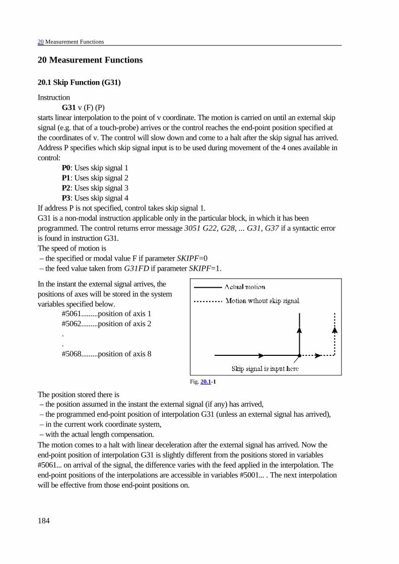
20 Measurement Functions
184
Fig. 20.1-1
20 Measurement Functions
20.1 Skip Function (G31)
InstructionG31 v (F) (P)
starts linear interpolation to the point of v coordinate. The motion is carried on until an external skipsignal (e.g. that of a touch-probe) arrives or the control reaches the end-point position specified atthe coordinates of v. The control will slow down and come to a halt after the skip signal has arrived.Address P specifies which skip signal input is to be used during movement of the 4 ones available incontrol:
P0: Uses skip signal 1P1: Uses skip signal 2P2: Uses skip signal 3P3: Uses skip signal 4
If address P is not specified, control takes skip signal 1.G31 is a non-modal instruction applicable only in the particular block, in which it has beenprogrammed. The control returns error message 3051 G22, G28, ... G31, G37 if a syntactic erroris found in instruction G31.The speed of motion is – the specified or modal value F if parameter SKIPF=0 – the feed value taken from G31FD if parameter SKIPF=1.
In the instant the external signal arrives, thepositions of axes will be stored in the systemvariables specified below.
#5061.........position of axis 1#5062.........position of axis 2..#5068.........position of axis 8
The position stored there is – the position assumed in the instant the external signal (if any) has arrived, – the programmed end-point position of interpolation G31 (unless an external signal has arrived), – in the current work coordinate system, – with the actual length compensation.The motion comes to a halt with linear deceleration after the external signal has arrived. Now theend-point position of interpolation G31 is slightly different from the positions stored in variables#5061... on arrival of the signal, the difference varies with the feed applied in the interpolation. Theend-point positions of the interpolations are accessible in variables #5001... . The next interpolationwill be effective from those end-point positions on.
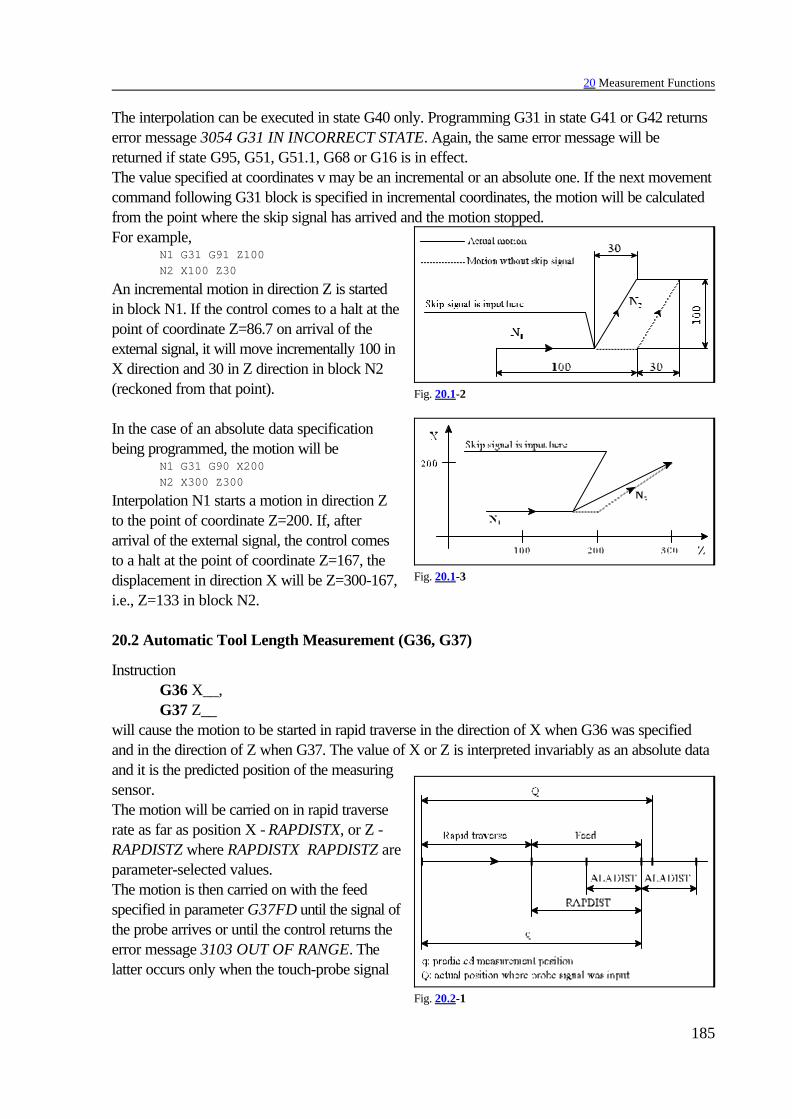
20 Measurement Functions
185
Fig. 20.1-2
Fig. 20.1-3
Fig. 20.2-1
The interpolation can be executed in state G40 only. Programming G31 in state G41 or G42 returnserror message 3054 G31 IN INCORRECT STATE. Again, the same error message will bereturned if state G95, G51, G51.1, G68 or G16 is in effect.The value specified at coordinates v may be an incremental or an absolute one. If the next movementcommand following G31 block is specified in incremental coordinates, the motion will be calculatedfrom the point where the skip signal has arrived and the motion stopped.For example,
N1 G31 G91 Z100N2 X100 Z30
An incremental motion in direction Z is startedin block N1. If the control comes to a halt at thepoint of coordinate Z=86.7 on arrival of theexternal signal, it will move incrementally 100 inX direction and 30 in Z direction in block N2(reckoned from that point).
In the case of an absolute data specificationbeing programmed, the motion will be
N1 G31 G90 X200N2 X300 Z300
Interpolation N1 starts a motion in direction Zto the point of coordinate Z=200. If, afterarrival of the external signal, the control comesto a halt at the point of coordinate Z=167, thedisplacement in direction X will be Z=300-167,i.e., Z=133 in block N2.
20.2 Automatic Tool Length Measurement (G36, G37)
InstructionG36 X__, G37 Z__
will cause the motion to be started in rapid traverse in the direction of X when G36 was specifiedand in the direction of Z when G37. The value of X or Z is interpreted invariably as an absolute dataand it is the predicted position of the measuringsensor.The motion will be carried on in rapid traverserate as far as position X - RAPDISTX, or Z -RAPDISTZ where RAPDISTX RAPDISTZ areparameter-selected values.The motion is then carried on with the feedspecified in parameter G37FD until the signal ofthe probe arrives or until the control returns theerror message 3103 OUT OF RANGE. Thelatter occurs only when the touch-probe signal
20 Measurement Functions
186
arrives outside of the ALADIST range (specified on parameter) of the predicted position X or Z.If the measurement is completed successfully and the touch-probe signal has arrived at the point ofcoordinate Q, the control will – add the difference Q-q to the wear compensation register selected earlier (if parameter ADD=1) – or will subtract the difference from it (if parameter ADD=0).The appropriate length compensation register have to be set up by programing Tnnmm prior tocommencement of the measurement. – G36, G37 are single-shot instructions. – Cycle G36, G37 will be executed invariably in the coordinate system of the current workpiece. – Parameters RAPDIST and ALADIST are always positive values. The condition RAPDIST >
ALADIST must be fulfilled for the two parameters. – Error message 3051 G22, G28, ... G31, G37 will be returned in the case of a syntactic error. – Code Tnnmm referring to a length compensation cannot be specified in block G37, or else error
message 3055 G37 IN INCORRECT STATE is returned. – Again, the same error message is returned when state G51, G51.1, G68 is in effect.
The following error message will be returned during the execution of function G36 or G37. – Message 3103 OUT OF RANGE is returned if the touch-probe signal arrives outside of the
ALADISTX or ALADISTZ range of the end position programmed in interpolation G36,G37.
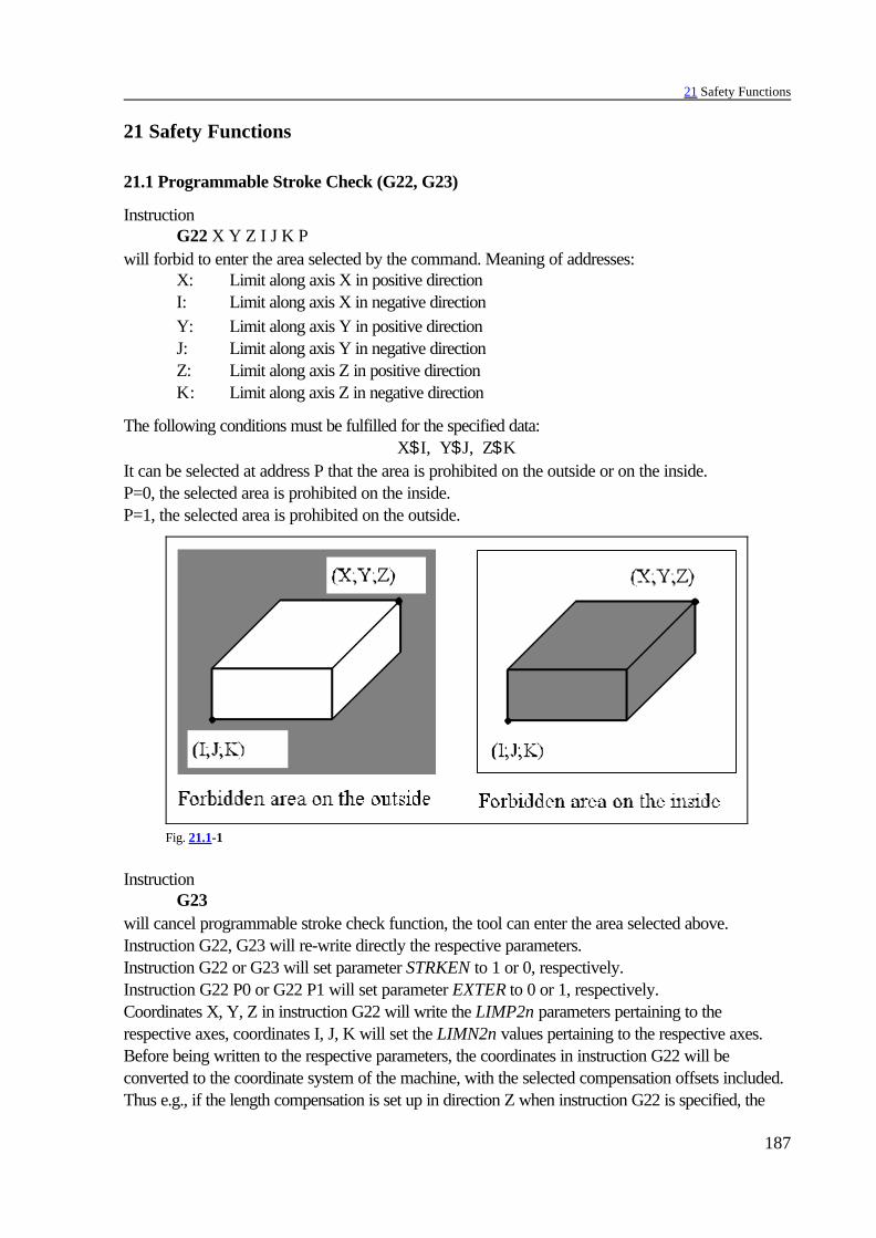
21 Safety Functions
187
Fig. 21.1-1
21 Safety Functions
21.1 Programmable Stroke Check (G22, G23)
InstructionG22 X Y Z I J K P
will forbid to enter the area selected by the command. Meaning of addresses:X: Limit along axis X in positive directionI: Limit along axis X in negative directionY: Limit along axis Y in positive directionJ: Limit along axis Y in negative directionZ: Limit along axis Z in positive directionK: Limit along axis Z in negative direction
The following conditions must be fulfilled for the specified data:X$I, Y$J, Z$K
It can be selected at address P that the area is prohibited on the outside or on the inside.P=0, the selected area is prohibited on the inside.P=1, the selected area is prohibited on the outside.
InstructionG23
will cancel programmable stroke check function, the tool can enter the area selected above.Instruction G22, G23 will re-write directly the respective parameters.Instruction G22 or G23 will set parameter STRKEN to 1 or 0, respectively.Instruction G22 P0 or G22 P1 will set parameter EXTER to 0 or 1, respectively.Coordinates X, Y, Z in instruction G22 will write the LIMP2n parameters pertaining to therespective axes, coordinates I, J, K will set the LIMN2n values pertaining to the respective axes.Before being written to the respective parameters, the coordinates in instruction G22 will beconverted to the coordinate system of the machine, with the selected compensation offsets included.Thus e.g., if the length compensation is set up in direction Z when instruction G22 is specified, the
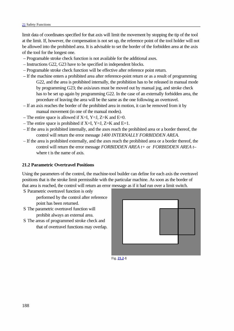
21 Safety Functions
188
Fig. 21.2-1
limit data of coordinates specified for that axis will limit the movement by stopping the tip of the toolat the limit. If, however, the compensation is not set up, the reference point of the tool holder will notbe allowed into the prohibited area. It is advisable to set the border of the forbidden area at the axisof the tool for the longest one. – Programable stroke check function is not available for the additional axes. – Instructions G22, G23 have to be specified in independent blocks. – Programable stroke check function will be effective after reference point return. – If the machine enters a prohibited area after reference-point return or as a result of programming
G22, and the area is prohibited internally, the prohibition has to be released in manual modeby programming G23; the axis/axes must be moved out by manual jog, and stroke checkhas to be set up again by programming G22. In the case of an externally forbidden area, theprocedure of leaving the area will be the same as the one following an overtravel.
– If an axis reaches the border of the prohibited area in motion, it can be removed from it bymanual movement (in one of the manual modes).
– The entire space is allowed if X=I, Y=J, Z=K and E=0. – The entire space is prohibited if X=I, Y=J, Z=K and E=1. – If the area is prohibited internally, and the axes reach the prohibited area or a border thereof, the
control will return the error message 1400 INTERNALLY FORBIDDEN AREA. – If the area is prohibited externally, and the axes reach the prohibited area or a border thereof, the
control will return the error message FORBIDDEN AREA t+ or FORBIDDEN AREA t– where t is the name of axis.
21.2 Parametric Overtravel Positions
Using the parameters of the control, the machine-tool builder can define for each axis the overtravelpositions that is the stroke limit permissible with the particular machine. As soon as the border ofthat area is reached, the control will return an error message as if it had run over a limit switch. S Parametric overtravel function is only
performed by the control after referencepoint has been returned.
S The parametric overtravel function willprohibit always an external area.
S The areas of programmed stroke check andthat of overtravel functions may overlap.
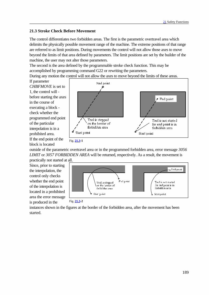
21 Safety Functions
189
Fig. 21.3-1
Fig. 21.3-2
21.3 Stroke Check Before Movement
The control differentiates two forbidden areas. The first is the parametric overtravel area whichdelimits the physically possible movement range of the machine. The extreme positions of that rangeare referred to as limit positions. During movements the control will not allow those axes to movebeyond the limits of that area defined by parameters. The limit positions are set by the builder of themachine, the user may not alter those parameters. The second is the area defined by the programmable stroke check function. This may beaccomplished by programming command G22 or rewriting the parameters. During any motion the control will not allow the axes to move beyond the limits of these areas.If parameterCHBFMOVE is set to1, the control will -before starting the axesin the course ofexecuting a block -check whether theprogrammed end pointof the particularinterpolation is in aprohibited area.If the end point of theblock is locatedoutside of the parametric overtravel area or in the programmed forbidden area, error message 3056LIMIT or 3057 FORBIDDEN AREA will be returned, respectively. As a result, the movement ispractically not started at all.Since, prior to startingthe interpolation, thecontrol only checkswhether the end pointof the interpolation islocated in a prohibitedarea the error messageis produced in theinstances shown in the figures at the border of the forbidden area, after the movement has beenstarted.
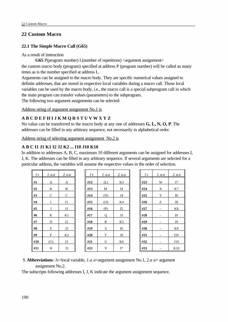
22 Custom Macro
190
22 Custom Macro
22.1 The Simple Macro Call (G65)
As a result of instructionG65 P(program number) L(number of repetitions) <argument assignment>
the custom macro body (program) specified at address P (program number) will be called as manytimes as is the number specified at address L.Arguments can be assigned to the macro body. They are specific numerical values assigned todefinite addresses, that are stored in respective local variables during a macro call. Those localvariables can be used by the macro body, i.e., the macro call is a special subprogram call in whichthe main program can transfer values (parameters) to the subprogram.The following two argument assignments can be selected:
Address string of argument assignment No.1 is
A B C D E F H I J K M Q R S T U V W X Y ZNo value can be transferred to the macro body at any one of addresses G, L, N, O, P. Theaddresses can be filled in any arbitrary sequence, not necessarily in alphabetical order.
Address string of selecting argument assignment No.2 is
A B C I1 J1 K1 I2 J2 K2 ... I10 J10 K10In addition to addresses A, B, C, maximum 10 different arguments can be assigned for addresses I,J, K. The addresses can be filled in any arbitrary sequence. If several arguments are selected for aparticular address, the variables will assume the respective values in the order of selection.
l v 1. a a 2. a a l v 1. a a 2. a a l v 1. a a 2. a a
#1 A A #12 (L) K3 #23 W J7
#2 B B #13 M I4 #24 X K7
#3 C C #14 (N) J4 #25 Y I8
#4 I I1 #15 (O) K4 #26 Z J8
#5 J J1 #16 (P) I5 #27 – K8
#6 K K1 #17 Q J5 #28 – I9
#7 D I2 #18 R K5 #29 – J9
#8 E J2 #19 S I6 #30 – K9
#9 F K2 #20 T J6 #31 – I10
#10 (G) I3 #21 U K6 #32 – J10
#11 H J3 #22 V I7 #33 – K10
S Abbreviations : lv=local variable, 1.a a=argument assignment No.1, 2.a a= argumentassignment No.2.
The subscripts following addresses I, J, K indicate the argument assignment sequence.

22 Custom Macro
191
The control will accept simultaneous selections of arguments 1 and 2 in a given block. An errormessage will be returned when an attempt is made to make reference twice to a variable of aparticular number. For example,
In the above example, variable #8 has already been assigned a value by the second address J(value, -12), since the value of address E is also assigned to variable #8, the control returns errormessage 3064 BAD MACRO STATEMENT.A decimal point and a sign can also be transferred at the addresses.
22.2 The Macro Modal Call
22.2.1 Macro Modal Call in Every Motion Command (G66)
As a result of instructionG66 P(program number) L(number of repetitions) <argument assignment>
the macro body specified at address P (program number) will be called after the execution of eachmotion command, as many times as is the number specified at address L. The interpretations ofaddresses P and L and the rules of argument assignment are identical with those described forinstruction G65.The selected macro will be called until with command
G67it is canceled.
For example, a hole has to be drilled in a given segment of the part program after each movement:
Main program
Macro body
%O1250 G0 Z#18 (rapid-traverse positioning in direction Z to the
point specified at address R–1)
G65 A2.12 B3.213 J36.9 J–12 E129.73 P2200
Variable#1=2.12#2=3.213#5=36.9#8=–12#8=Error
...G66 P1250 Z–100 R–1 X2 F130 (Z=Z point of hole, R=R point of hole,
X=dwell F=feed)G91 G0 X100Y30 drilling is performed after each posi-
tioning X150...G67

22 Custom Macro
192
G1 Z#26 F#9 (drilling as far as the point Z specified ataddress Z–100, with the feed specified at addressF130)
G4 P#24 (dwell at the bottom of the hole for the timespecified at address X2)
G0 Z-[#18+#26] (retraction of the tool to the initial point) M99 (return to the main program) %
22.2.2 Macro Modal Call From Each Block (G66.1)
As a result of commandG66.1 P(program number) L(number of repetitions) <argument assignment>
all subsequent blocks will be interpreted as argument assignment, and the macro of the numberspecified at address P will be called, and will be executed as many times as is the number specifiedat address L.The command produces the same effect as if each block were a G65 macro call:
The selected macro will be called until with commandG67
it is canceled.
The rules of argument assignment are
1. In the block performing the activation (in which G66.1 P L has been programmed), the rulesof the argument assignment are the same as in command G65.
2. In the blocks following instruction G66.1,the same addresses can be used as in command G65, andL: #12,P: #16,G: #10 with the qualification that the control will accept only one reference to an address G
in each block; programming several G addresses will produce error message 3005ILLEGAL G CODE.
N: #14 if an N address is at the beginning of a block (or preceded at most by the address ofa conditional block "/"), the second N address will be considered for an argument:
If address N is in the middle of the block (preceded by any address other than "/"),address N will be interpreted as an argument:
G66.1 P LX Y Z G65 P L X Y ZM S = G65 P L M SX G65 P L XG67
/N130 X12.3 Y32.6 N250
Block No.#24=12.3#25=32.6#14=250
X34.236 N320
#24=34.236#14=320
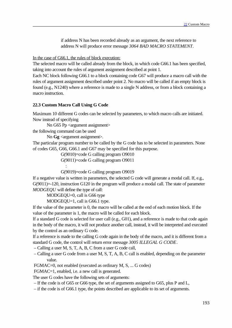
22 Custom Macro
193
if address N has been recorded already as an argument, the next reference toaddress N will produce error message 3064 BAD MACRO STATEMENT.
In the case of G66.1, the rules of block execution:The selected macro will be called already from the block, in which code G66.1 has been specified,taking into account the rules of argument assignment described at point 1.Each NC block following G66.1 to a block containing code G67 will produce a macro call with therules of argument assignment described under point 2. No macro will be called if an empty block isfound (e.g., N1240) where a reference is made to a single N address, or from a block containing amacro instruction.
22.3 Custom Macro Call Using G Code
Maximum 10 different G codes can be selected by parameters, to which macro calls are initiated.Now instead of specifying
Nn G65 Pp <argument assignment>the following command can be used
Nn Gg <argument assignment>.The particular program number to be called by the G code has to be selected in parameters. Noneof codes G65, G66, G66.1 and G67 may be specified for this purpose.
G(9010)=code G calling program O9010G(9011)=code G calling program O9011 :G(9019)=code G calling program O9019
If a negative value is written in parameters, the selected G code will generate a modal call. If, e.g.,G(9011)=-120, instruction G120 in the program will produce a modal call. The state of parameterMODGEQU will define the type of call:
MODGEQU=0, call is G66 typeMODGEQU=1, call is G66.1 type.
If the value of the parameter is 0, the macro will be called at the end of each motion block. If thevalue of the parameter is 1, the macro will be called for each block.If a standard G code is selected for user call (e.g., G01), and a reference is made to that code againin the body of the macro, it will not produce another call, instead, it will be interpreted and executedby the control as an ordinary G code.If a reference is made to the calling G code again in the body of the macro, and it is different from astandard G code, the control will return error message 3005 ILLEGAL G CODE. – Calling a user M, S, T, A, B, C from a user G code call, – Calling a user G code from a user M, S, T, A, B, C call is enabled, depending on the parameter
value. FGMAC=0, not enabled (executed as ordinary M, S, ... G codes) FGMAC=1, enabled, i.e. a new call is generated.The user G codes have the following sets of arguments: – If the code is of G65 or G66 type, the set of arguments assigned to G65, plus P and L, – if the code is of G66.1 type, the points described are applicable to its set of arguments.

22 Custom Macro
194
A modal code can be deleted by instruction G67.
22.4 Custom Macro Call Using M Code
Maximum 10 different M codes can be selected by parameters, to which macro calls are initiated.Now the series of instructions
Nn Mm <argument assignment>have to be typed. Now code M will not be transferred to the PLC, but the macro of the respectiveprogram number will be called.The particular program number to be called by the calling M code has to be selected by parameters.
M(9020)=code M calling program O9020M(9021)=code M calling program O9021 :M(9029)=code M calling program O9029
Code M can specify invariably a type G65 call (i.e., a non-modal one).If reference is made again to the same M code in the middle of the macro body, the latter will notcall the macro, instead, M code will be transferred to the PLC.If a user call type G, S, T, A, B, C or some other user call type M is made in the middle of themacro body,
FGMAC=0, not enabled (executed as ordinary M, S, ... G codes)FGMAC=1, enabled, i.e. a new call is generated.
An M code selected by parameters to initiate a macro call may be preceded only by "/" and addressN in the block.A block containing a macro call initiated by M code may include a single M code only.Set of arguments No.1:
A B C D E F G H I J K L P Q R S T U V W X Y ZSet of arguments No. 2 also can be used with function M.
22.5 Subprogram Call with M Code
Maximum 10 M codes can be selected by parameters, by which subprogram calls can be initiated.Now instead of instruction
Nn Gg Xx Yy M98 Ppcan be specified
Nn Gg Xx Yy MmNow the selected M code will not be transferred to the PLC, instead, the respective subprogramwill be called.The particular program number to be called by M code can be selected by the followingparameters.
M(9000)=code M calling program O9000M(9001)=code M calling program O9001 :M(9009)=code M calling program O9009
If reference is made to the same M code again in the subprogram, the latter will not call thesubprogram again, but M code will be transferred to the PLC.If a user call G, S, T, A, B, C or some other user call M is made in the subprogram:
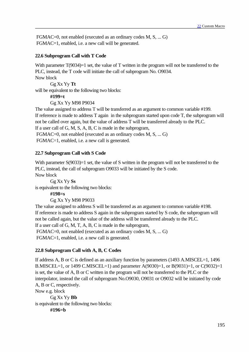
22 Custom Macro
195
FGMAC=0, not enabled (executed as an ordinary codes M, S, ... G) FGMAC=1, enabled, i.e. a new call will be generated.
22.6 Subprogram Call with T Code
With parameter T(9034)=1 set, the value of T written in the program will not be transferred to thePLC, instead, the T code will initiate the call of subprogram No. O9034.Now block
Gg Xx Yy Ttwill be equivalent to the following two blocks:
#199=tGg Xx Yy M98 P9034
The value assigned to address T will be transferred as an argument to common variable #199.If reference is made to address T again in the subprogram started upon code T, the subprogram willnot be called over again, but the value of address T will be transferred already to the PLC.If a user call of G, M, S, A, B, C is made in the subprogram, FGMAC=0, not enabled (executed as an ordinary codes M, S, ... G) FGMAC=1, enabled, i.e. a new call is generated.
22.7 Subprogram Call with S Code
With parameter S(9033)=1 set, the value of S written in the program will not be transferred to thePLC, instead, the call of subprogram O9033 will be initiated by the S code.Now block
Gg Xx Yy Ssis equivalent to the following two blocks:
#198=sGg Xx Yy M98 P9033
The value assigned to address S will be transferred as an argument to common variable #198.If reference is made to address S again in the subprogram started by S code, the subprogram willnot be called again, but the value of the address will be transferred already to the PLC.If a user call of G, M, T, A, B, C is made in the subprogram, FGMAC=0, not enabled (executed as an ordinary codes M, S, ... G) FGMAC=1, enabled, i.e. a new call is generated.
22.8 Subprogram Call with A, B, C Codes
If address A, B or C is defined as an auxiliary function by parameters (1493 A.MISCEL=1, 1496B.MISCEL=1, or 1499 C.MISCEL=1) and parameter A(9030)=1, or B(9031)=1, or C(9032)=1is set, the value of A, B or C written in the program will not be transferred to the PLC or theinterpolator, instead the call of subprogram No.O9030, O9031 or O9032 will be initiated by codeA, B or C, respectively.Now e.g. block
Gg Xx Yy Bbis equivalent to the following two blocks:
#196=b

22 Custom Macro
196
Gg Xx Yy M98 P9031The values assigned to addresses A, B and C will be transferred to common variables #195, #196,and #197, respectively. If reference is made again to the same address in the subprogram started by code A, B or C, thesubprogram will not be called again, but the value of the address will be transferred already to thePLC or interpolator.If a call of a user G, M, S, T code is made in the subprogram, FGMAC=0, not enabled (executed as ordinary codes M, S, ... G) FGMAC=1, enabled, i.e. a new call is generated.
22.9 Differences Between the Call of a Sub-Program and the Call of a Macro
– A macro call may include arguments, but a subprogram call may not. – The call of a subprogram will only branch into the subprogram after the execution of other
commands programmed in the block; a macro call will branch only. – A macro call will alter the levels of local variables, a subprogram call will not. For example, the
value of #1 prior to the call of G65 is different from the one in the middle of macro body.The value of #1 before M98 is identical with that in the subprogram.
22.9.1 Multiple Calls
Another macro can be called again from a macro. Macro calls can be made in four levels of depth,including simple and modal ones. With the subprogram calls included, the maximum depth of thecalls may cover 8 levels.In the case of multiple calls of modal macros (type G66), first the latter specified macro will becalled after execution of each interpolation block, from which the previously specified macros will becalled in a backward sequence. Let us see the example below:
%O0001 ... N10 G66 P2 N11 G1 G91 Z10 (1–11) N12 G66 P3 N13 Z20 (1–13) N14 G67 (canceling of call G66 P3...) N15 G67 (canceling of call G66 P2 ...) N16 Z–5 (1–16) ...
%O0002 N20 X4 (2–20) N21 M99 %
%O0003 N30 Z2 (3–30) N31 Z3 (3–31) N32 M99 %

22 Custom Macro
197
Including only the interpolations, the sequence of execution will be
Of the numbers in brackets, the first and the second ones are the numbers of the programs andblock being executed, respectively.Instruction G67 specified in block N14 will cancel the macro called in block N12 (O0003); the onespecified in block N15 will cancel the macro called in block N10 (O0002).In the case of multiple calls of macros type G66.1, first the last specified macro will be called inentering each block (treating the addresses of the particular block as arguments), then the previouslyspecified macro will be called, entering the blocks of that macro and treating them as arguments.If another macro is called again from a macro, the levels of local variables will also increase with themacro levels.
main program macro macro macro macrolevel 0 level 1 level 2 level 3 level 4 O_____ O_____ O_____ O_____
G65 P G65 P G65 P G65 P
M99 M99 M99 M99
local variableslevel 0 level 1 level 2 level 3 level 4#1 #1 #1 #1 #1 : : : :#33 #33 #33 #33 #33
When the first macro is called, the local variables of the main program will be stored (#1 through#33), and the local variables at level 1 will assume the argument values specified in the call. Ifanother macro is called from the first level, the local variables of the first level will be stored (#1through #33), and the local variables on the second level will assume the argument values specifiedin the call. In the case of multiple call, the local variables of the previous level will be stored and thelocal variables on the next level will assume the argument values specified in the call. In the case ofM99, returning from the called macro to the calling program, the local variables stored on theprevious level will be restored in the same states they were at the time of being stored during the call.
(1–11) (1–13) (1–16) Level of call))) Level 0
(2–20) (3–30) (3–31)))) Level 1
(2–20) (2–20)))) Level 2

22 Custom Macro
198
22.10 Format of Custom Macro Body
The program format of a user macro is identical with that of a subprogram:O(program number):commands:M99
The program number is irrelevant, but the program numbers between O9000 and O9034 arereversed for special calls.
22.11 Variables of the Programming Language
Variables instead of specific numerical values can be assigned to the addresses in the mainprograms, subprograms and macros. A value can be assigned to each variable within the permissiblerange. The use of variables will make for much more flexible procedures of programming.The appropriate data can be parametrized by the use of common variables in the main programs andsubprograms, thus it will not be necessary to write new programs for similar work parts of differentsize. Instead, the operator can change to new part of different size by re-writing the appropriatecommon variables.The use of variables can make a macro much more flexible than a conventional subprogram.Whereas arguments cannot be transferred to a subprogram, arguments can be attached to a macrothrough the local variables.
22.11.1 Identification of a Variable
A number of variables can be used, and each will be identified by its number. A variable iscomposed of the code # and a number. For example,
#12#138#5106
A formula may also be used to make reference to variable - #[<formula>]For example,
#[#120] means that variable 120 contains the serial number of variable that is referred to;#[#120-4] means that the referred variable number is obtained by subtracting 4 from the
number contained in the variable.
22.11.2 Referring to a Variable
The various addresses in the words of a program block can assume values of variables as well asnumerical values. The minus sign ("–") or operator I can, wherever it is permissible with numericalvalues, be used even when a reference is made to a variable after an address. For example,
G#102 if #102=1.0, this reference is equivalent to G1XI–#24 if #24=135.342, this reference is equivalent to XI–135.342
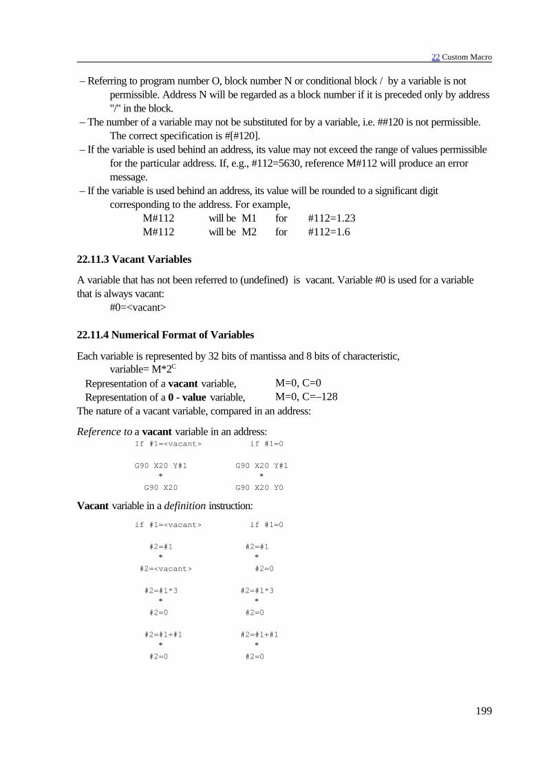
22 Custom Macro
199
– Referring to program number O, block number N or conditional block / by a variable is notpermissible. Address N will be regarded as a block number if it is preceded only by address"/" in the block.
– The number of a variable may not be substituted for by a variable, i.e. ##120 is not permissible.The correct specification is #[#120].
– If the variable is used behind an address, its value may not exceed the range of values permissiblefor the particular address. If, e.g., #112=5630, reference M#112 will produce an errormessage.
– If the variable is used behind an address, its value will be rounded to a significant digitcorresponding to the address. For example,
M#112 will be M1 for #112=1.23M#112 will be M2 for #112=1.6
22.11.3 Vacant Variables
A variable that has not been referred to (undefined) is vacant. Variable #0 is used for a variablethat is always vacant:
#0=<vacant>
22.11.4 Numerical Format of Variables
Each variable is represented by 32 bits of mantissa and 8 bits of characteristic,variable= M*2C
Representation of a vacant variable, M=0, C=0 Representation of a 0 - value variable, M=0, C=–128The nature of a vacant variable, compared in an address:
Reference to a vacant variable in an address: If #1=<vacant> if #1=0
G90 X20 Y#1 G90 X20 Y#1 * * G90 X20 G90 X20 Y0
Vacant variable in a definition instruction:
if #1=<vacant> if #1=0
#2=#1 #2=#1 * * #2=<vacant> #2=0
#2=#1*3 #2=#1*3 * * #2=0 #2=0
#2=#1+#1 #2=#1+#1 * * #2=0 #2=0

22 Custom Macro
200
Difference between a vacant variable and a 0 - value one in a conditional expression will be
if #1=<vacant> if #1=0
#1 EQ #0 #1 EQ #0 * * fulfilled not fulfilled
#1 NE 0 #1 NE 0 * * fulfilled not fulfilled
#1 GE #0 #1 GE #0 * * fulfilled not fulfilled
#1 GT 0 #1 GT 0 * *
fulfilled not fulfilled
22.12 Types of Variables
With reference to the ways of their uses and their properties, the variables are classified into local,common and system variables. The number of the variables tells the particular category to which itpertains.
22.12.1 Local Variables (#1 through #33)
The local variable is a variable used by the macro program locally. If macro A calls B, and referenceis made to local variable #i in each of macros A and B, the value of local variable #i at the levelmacro A will not be lost and will not be re-written after macro B has been called - despite the factthat reference is made to #i in macro B as well. The local variables are used for the transfer ofarguments. The matches between the addresses of arguments and the local variables are containedin the Table in the Section describing the procedure of a simple macro call (G65).The local variable whose address has not been involved in the argument assignment, is a vacant onethat can be used optionally.
22.12.2 Common Variables (#100 through #199, #500 through #599)
Unlike the local variables, the common variables are identical throughout the entire program (notonly at the given levels of program calls) - regardless of whether they are in the main program, asubprogram or in a macro, or at whatever level of the macro. If accordingly, #i has been used in amacro, e.g. a value has been assigned to it, #i will have the same value in another macro, too, until itis re-written. The common variables can be used absolutely freely in the system, they have nodistinguished functions at all.
The common variables from #100 to #199 will be deleted upon a power-off. The values of common variables #500 through #599 will be preserved even after a power-off.The macro variables #500 through #599 can be made "write-protected" by the use of parametersWRPROT1 and WRPROT2. The number of the first and the last element of the block to be
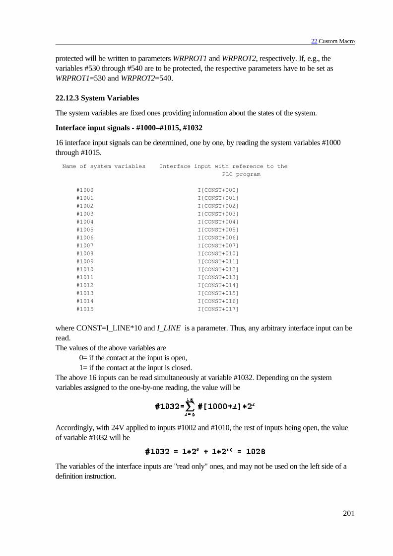
22 Custom Macro
201
protected will be written to parameters WRPROT1 and WRPROT2, respectively. If, e.g., thevariables #530 through #540 are to be protected, the respective parameters have to be set asWRPROT1=530 and WRPROT2=540.
22.12.3 System Variables
The system variables are fixed ones providing information about the states of the system.
Interface input signals - #1000–#1015, #1032
16 interface input signals can be determined, one by one, by reading the system variables #1000through #1015.
Name of system variables Interface input with reference to the PLC program
#1000 I[CONST+000] #1001 I[CONST+001] #1002 I[CONST+002] #1003 I[CONST+003] #1004 I[CONST+004] #1005 I[CONST+005] #1006 I[CONST+006] #1007 I[CONST+007] #1008 I[CONST+010] #1009 I[CONST+011] #1010 I[CONST+012] #1011 I[CONST+013] #1012 I[CONST+014] #1013 I[CONST+015] #1014 I[CONST+016] #1015 I[CONST+017]
where CONST=I_LINE*10 and I_LINE is a parameter. Thus, any arbitrary interface input can beread.The values of the above variables are
0= if the contact at the input is open,1= if the contact at the input is closed.
The above 16 inputs can be read simultaneously at variable #1032. Depending on the systemvariables assigned to the one-by-one reading, the value will be
Accordingly, with 24V applied to inputs #1002 and #1010, the rest of inputs being open, the valueof variable #1032 will be
The variables of the interface inputs are "read only" ones, and may not be used on the left side of adefinition instruction.

22 Custom Macro
202
Interface output signals - #1100–#1115, #1132
16 interface output signals can be issued, one by one, by assigning values to variables #1100through #1115.
Name of system variables Interface input with reference to the PLC program
#1100 Y[CONST+000] #1101 Y[CONST+001] #1102 Y[CONST+002] #1103 Y[CONST+003] #1104 Y[CONST+004] #1105 Y[CONST+005] #1106 Y[CONST+006] #1107 Y[CONST+007] #1108 Y[CONST+010] #1109 Y[CONST+011] #1110 Y[CONST+012] #1111 Y[CONST+013] #1112 Y[CONST+014] #1113 Y[CONST+015] #1114 Y[CONST+016] #1115 Y[CONST+017]
where CONST=O_LINE*10 and O_LINE is a parameter. Thus, any arbitrary interface outputword can be issued or read.The values of the above variables may be
0= the contact at the output is open,1= the contact at the output is closed.
The above 16 outputs can be issued simultaneously by using variable #1132. Depending on thesystem variables assigned to the single outputs, the output value will be
Accordingly, with outputs #1102 and #1109 are on, the rest of outputs being off, variable #1132must output the value

22 Custom Macro
203
Tool compensation values - #10001 through #13999
The tool compensation values can be read from variables #10001 through #19999, or values can beassigned them.
N X Y Z R Q
wear geom.. wear geom.. wear geom.. wear geom..
1 #10001 #15001 #14001 #19001 #11001 #16001 #12001 #17001 #13001
2 #10002 #15002 #14002 #19002 #11002 #16002 #12002 #17002 #13002
... ... ... ... ... ... ... ... ... ...
99 #10099 #15099 #14099 #19099 #11099 #16099 #12099 #17099 #13099
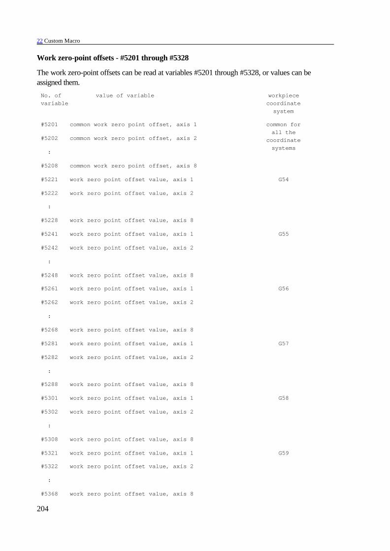
22 Custom Macro
204
Work zero-point offsets - #5201 through #5328
The work zero-point offsets can be read at variables #5201 through #5328, or values can beassigned them.
No. of value of variablevariable
workpiececoordinatesystem
#5201 common work zero point offset, axis 1 common forall the
coordinatesystems
#5202 common work zero point offset, axis 2
:
#5208 common work zero point offset, axis 8
#5221 work zero point offset value, axis 1 G54
#5222 work zero point offset value, axis 2
:
#5228 work zero point offset value, axis 8
#5241 work zero point offset value, axis 1 G55
#5242 work zero point offset value, axis 2
:
#5248 work zero point offset value, axis 8
#5261 work zero point offset value, axis 1 G56
#5262 work zero point offset value, axis 2
:
#5268 work zero point offset value, axis 8
#5281 work zero point offset value, axis 1 G57
#5282 work zero point offset value, axis 2
:
#5288 work zero point offset value, axis 8
#5301 work zero point offset value, axis 1 G58
#5302 work zero point offset value, axis 2
:
#5308 work zero point offset value, axis 8
#5321 work zero point offset value, axis 1 G59
#5322 work zero point offset value, axis 2
:
#5368 work zero point offset value, axis 8
22 Custom Macro
205
The axis number refers to the physical ones. The relationship between the numbers and the names ofaxes will be defined by the machine tool builder by parameters in group AXIS. Usually axes 1, 2 and3 are assigned to addresses X, Y and Z, respectively, but different specifications are also permissible.
Alarm - #3000
By defining#3000=nnn(ALARM),
a numerical error message (nnn=max. three decimal digits) and the text of error message can beprovided. The text must be put in (,) brackets. A message may not be longer than 25 characters.If the macro contains an error, i.e., the program runs to a branch in which a value has been defined tovariable #3000, the program will be executed as far as the previous block, then the execution issuspended and the error message and the code of it (4nnn) are displayed on the screen. The numberof the message is the sum of number specified on #3000 variable and 4000. If no number was specified,the code of the message would be 4000 if no text was specified the message field will be empty. Theerror state can be canceled by the RESET button.
Millisecond timer - #3001
The value of variable #3001 can be read and written.The time interval between two time instants can be measured in milliseconds, with an accuracy of about20 ms. Counter #3001 will overflow at 65536. The value of variable #3001 will start from zero at thetime of power-on, and will count upwards. Counting is continuous as long as the control is on.
Main time timer - #3002
The value of variable #3002 can be read and written.The time interval between two time instants can be measured in minutes, with an accuracy of about 20ms.At the time of power-on, the value of variable #3002 will start at the power-off level and will be countedupwards.Counting is on as long as the START light is on, i.e., the time is being measured in the start conditionof the control. It is located at time meter CUTTING2 of the parameter memory.
Suppression of block-by-block execution - #3003
If #3003=1, the control will not stop on completion of a block (in the state of single block mode) untilthat variable assumes value 0.The value of the variable is 0 at power-off or after resetting the program to its beginning.
#3003 block-by-block execution 0 = not suppressed 1 = suppressed

22 Custom Macro
206
Suppression of stop button, feed override, exact stop - #3004
Under the conditions of suppression of feed stop function, the feed will stop after the stop button ispressed when the suppression is released.When the feedrate override is suppressed, the override takes the value of 100% until the suppressionis released.Under the conditions of the suppression of the exact stop, the control will not perform a check until thesuppression has been released.The value of the variable is 0 at power-on or after resetting the program to its beginning.
#3004 Exact stop Feed override Feed stop 0 0 0 0 1 0 0 1 2 0 1 0 3 0 1 1 4 1 0 0 5 1 0 1 6 1 1 0 7 1 1 1
0 = function is effective1 = function is suppressed
Stop with message - #3006
As a result of a value assigned to#3006=nnn(MESSAGE)
the execution of the program is stopped, and the message in round brackets and the code 5nnn will bedisplayed on the screen. The code is the sum of the number specified on the variable and 5000. If nonumber was specified, code 5000 would be displayed, if no text was specified message field would beempty. The execution of the program is resumed upon depression of the START button, then themessage is cleared from the screen. The message may not be longer than 25 characters. This instructionis useful whenever the operator's intervention is needed during the execution of the program.
Mirror image status - #3007
By reading variable #3007, the operator can establish the particular physical axis, on which mirror-image command is recorded. This variable is a "read only" one.The value of the variable is interpreted in binary terms as follows.1 1 1 1 1 15 4 3 2 1 0 9 8 7 6 5 4 3 2 1 0
Axis 1Axis 2Axis 3
Axis 8

22 Custom Macro
207
The bits have the following meanings:0 = no mirror imaging1 = mirror imaging on.
If, e.g., the value of the variable is 5, mirror image is on in axes 1 and 3. The axis number refers to aphysical axis, the parameter defining the particular name of axis pertaining to a physical axis number.
Number of machined parts, number of parts to be machined - #3901, #3902
The numbers of machined parts are collected in counter #3901 by the control. The contents of thecounter will be incremented by 1 upon the execution of each function M02, M30 or selected Mfunctions in parameter PRTCNTM. As soon as the number of machined parts becomes equal to therequired number of parts (counter #3902), the NC tells it the PLC on a flag.
Number of machined parts #3901Number of parts to be machined #3902
Counters #3901 and #3902 are located on parameters PRTTOTAL and PRTREQRD, respectively.
Modal information - #4001 through #4130, #4201 through #4330
The modal values effective in the previous block can be established by reading system variables #4001through #4130.The modal commands effective in the block under execution can be established by reading variables#4201 through 4330.
systemvariable
#4001:
#4020#4101#4102#4103#4107#4108#4109#4111#4113#4114#4115#4119#4120
modal information ofthe previous block
G code, group 1:
G code, group 20code Acode Bcode Ccode Dcode Ecode Fcode H
code M entered firstblock number, Nprogram number, O
code Scode T
*******************
systemvariable
#4201:
#4220#4301#4302#4303#4307#4308#4309#4311#4313#4314#4315#4319#4320
modal information ofthe block being
executed
G code, group 1:
G code, group 20code Acode Bcode Ccode Dcode Ecode Fcode H
code M entered firstblock number, Nprogram number, O
code Scode T

22 Custom Macro
208
Positional information - #5001 through #5108
Positions at block end system position information reading in during variable motion
#5001 block end coordinate of axis 1 #5002 block end coordinate of axis 2 : possible #5008 block end coordinate of axis 8
The block end coordinate will be entered in the variable – in the current work coordinate system – with the coordinate offsets taken into account – in Cartesian coordinates – With all compensations (length, radius, tool offset) ignored.
Instantaneous positions in the coordinate system of the machine
system nature of position information entry during variable motion
#5021 instantaneous coordinate of axis 1 (G53) #5022 instantaneous coordinate of axis 2 (G53) : not possible #5028 instantaneous coordinate of axis 8 (G53)
The instantaneous position (G53) will be entered in the variable – in machine coordinate system – with all compensations (length, radius, tool offset) taken into account.
Instantaneous positions in the work coordinate system
system nature of position information entry during variable motion
#5041 instantaneous coordinate of axis 1 #5042 instantaneous coordinate of axis 2 : not possible #5048 instantaneous coordinate of axis 8
The instantaneous coordinate of will be entered in the variable – in the current work coordinate system – with the coordinate offsets taken in account – in Cartesian coordinates – with all compensations (length, radius, tool offset) taken into account.

22 Custom Macro
209
Fig. 22.12.3-1
Skip signal position
system nature of position information entry during variable motion
#5061 Skip signal coordinate of axis 1 (G31) #5062 Skip signal coordinate of axis 2 (G31) : possible #5068 Skip signal coordinate of axis 8 (G31)
The position, in which the skip signal has arrived in block G31 will be entered in the variable – in the work coordinate system – with the coordinate offsets taken into account – in Cartesian coordinates – with all compensations (length, radius, tool offset) taken into account.Unless the skip signal has arrived, the above variables will assume the end-point position programmedin block G31.
Tool-length compensation
system nature of position information entry during variable motion
#5081 length compensation on axis 1 #5082 length compensation on axis 2 : not possible #5088 length compensation on axis 8
The readable tool-length compensation is the one in effect in the block being executed.

22 Custom Macro
210
Servo lag
system nature of position information entry during variable motion
#5101 servo lag in axis 1 #5102 servo lag in axis 2 : not possible #5108 servo lag in axis 8
The readable servo lag is a signed value in millimeters.
22.13 Instructions of the Programming Language
The expression#i = <formula>
is used for describing the various instructions. The expression <formula> may include arithmeticoperations, functions, variables or constants.In general, references are made to variables #j and #k in a <formula>.It is not only possible for the <formula> to stand on the right side of a definition instruction, the variousaddresses in the NC block may also assume a formula instead of a specific numerical value or variable.
22.13.1 Definition, Substitution: #i = #j
The code of instruction is =.As a result of the instruction, variable #i will assume the value of variable #j, i.e., the value of variable#j will be entered in variable #i.
22.13.2 Arithmetic Operations and Functions
Single-Operand Operations
Single-operand minus: #i = – #jThe code of the operation is –.As a result of the operation, variable #i will have a value identical with variable #j in absolutevalue but opposite in sign.
Arithmetic negation: #i = NOT #jThe code of the operation is NOTAs a result of the operation, variable #j is converted first into a 32-bit fixed-point number. Errormessage 3091 ERRONEOUS OPERATION WITH # is returned unless the converted numbercan be represented by 32 bits. Then the value of that fixed-point number will be negated bit bybit and the number produced this way will be re-converted into a floating-point one and will beput in variable #i.
Additive arithmetic operations
Addition: #i = #j + #kThe code of the operation is +.As a result of the operation, variable #i will assume the sum of the values of variables #j and #k.

22 Custom Macro
211
Subtraction: #i = #j – #kThe code of the operation is –.As a result of the operation, variable #i will assume the difference of the values of variables #jand #k.
Logical sum, or: #i = #j OR #kThe code of the operation is OR.As a result of operation, the logic sum of variables #j and #k will be entered in variable #i atevery bit of 32 bits. Wherever 0 is found at each of the identical bit values of the two numbers,0 will be represented by that bit value in the result (otherwise 1).
Exclusive or: #i = #j XOR #kThe code of the operation is XOR.As a result of operation, the variables #j and #k will be added together in every bit of 32 bitsin variable #i in such a way that 0 will be the bit value in the result wherever identical numericalvalues are found in identical bit positions (and 1 will be wherever different numerical values arefound), in each of the 32 bits.
Multiplicative arithmetic operations
Multiplication: #i = #j * #kThe code of the operation is *.As a result of operation, variable #i will assume the product of the values of variables #j and #k.
Division: #i = #j / #kThe code of the operation is /.As a result of operation, variable #i will assume the quotient of variables #j and #k. The valueof #k may not be 0 or else the control will return error message 3092 DIVISION BY 0 #.
Remainder: #i = #j MOD #kThe code of the operation is MOD.As a result of the operation, variable #i will assume the remainder of the quotient of variables#j and #k. The value of #k may not be 0 or else the control will return error message 3092DIVISION BY 0 #.Example: At #120 = 27 MOD 4, the value of variable #120 will be 3.
Logical product, and - i# = #j AND #kThe code of operation is AND.As a result of operation, the logical product of variables #j and #k will be entered in every bitof the 32 bits in variable #i. Wherever 1 is found at each of the identical bit position of twonumbers, 1 will be found there in the result, otherwise 0.
Functions
Square root: #i = SQRT #jThe code of operation is SQRT.As a result of operation, variable #i will assume the square root of variable #j. The value of #jmay not be a negative number.

22 Custom Macro
212
Sine: #i = SIN #jThe code of operation is SIN.As a result of operation, variable #i will assume the sine of variable #j. The value of #j alwaysrefers to degrees.
Cosine: #i = COS #jThe code of operation is COS.As a result of operation, variable #i will assume the cosine of variable #j. The value of #j alwaysrefers to degrees.
Tangent: #i = TAN #jThe code of operation is TAN.As a result of operation, variable #i will assume the tangent of variable #j. The value of #jalways refers to degrees. The value of #j may not be (2n+1)*90°, where n=0, ±1, ±2, ...
Arc sine: #i = ASIN #jThe code of the function is ASIN.As a result of operation, variable #i will assume the arc sine of variable #j in degrees. Thecondition –1##j#1 must be true. The result, i.e., the value of #i, lies between +90° and -90°.
Arc cosine: #i = ACOS #jThe code of the function is ACOS.As a result of operation, variable #i will assume the arc cosine of variable #j in degrees. Thecondition –1##j#1 must be true. The result, i.e. the value of #i, lies between 0° and 180°.
Arc tangent - #i = ATAN #jThe code of the function is ATAN.As a result of operation, variable #i will assume the arc tangent of variable #j in degrees. Theresult, i.e. the value of #i, lies between +90° and -90°.
Exponent with base e: #i = EXP #jThe code of the function is EXP.As a result of the operation, variable #i will assume the #j-th power of the natural number (e).
Logarithm natural: #i = LN #jThe code of the function is LN.As a result of operation, variable #i will assume the logarithm natural of number #j. The valueof #j may not be 0 or a negative number.
Absolute value: #i = ABS #jThe code of the function is ABS.As a result of operation, variable #i will assume the absolute value of variable #j.
Conversion from binary into binary-coded decimal: #i = BCD #jThe code of the function is BCD.As a result of operation, variable #i will assume the BCD value of variable #j. The value rangeof variable #j is 0 to 99999999.
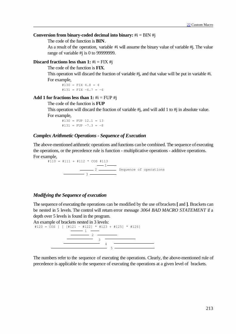
22 Custom Macro
213
Conversion from binary-coded decimal into binary: #i = BIN #jThe code of the function is BIN.As a result of the operation, variable #i will assume the binary value of variable #j. The valuerange of variable #j is 0 to 99999999.
Discard fractions less than 1: #i = FIX #jThe code of the function is FIX.This operation will discard the fraction of variable #j, and that value will be put in variable #i.For example,
#130 = FIX 4.8 = 4#131 = FIX –6.7 = –6
Add 1 for fractions less than 1: #i = FUP #jThe code of the function is FUPThis operation will discard the fraction of variable #j, and will add 1 to #j in absolute value.For example,
#130 = FUP 12.1 = 13#131 = FUP –7.3 = –8
Complex Arithmetic Operations - Sequence of Execution
The above-mentioned arithmetic operations and functions can be combined. The sequence of executingthe operations, or the precedence rule is function - multiplicative operations - additive operations.For example,
Modifying the Sequence of execution
The sequence of executing the operations can be modified by the use of brackets [ and ]. Brackets canbe nested in 5 levels. The control will return error message 3064 BAD MACRO STATEMENT if adepth over 5 levels is found in the program.An example of brackets nested in 3 levels:
The numbers refer to the sequence of executing the operations. Clearly, the above-mentioned rule ofprecedence is applicable to the sequence of executing the operations at a given level of brackets.
#110 = #111 + #112 * COS #1131
2 Sequence of operations3
#120 = COS [ [ [#121 - #122] * #123 + #125] * #126]1
23
45

22 Custom Macro
214
22.13.3 Logical Operations
The programming language uses the following logical operations:
Equal to #i EQ #j
Not equal to #i NE #j
Greater than #i GT #j
Less than #i LT #j
Greater than or equal to #i GE #j
Less than or equal to #i LE #jThe variables on both sides of a logical operation can be substituted by formula as well. The aboveconditional expressions can be used in divergence or iteration instructions IF or WHILE. L Note: Since the above conditional expressions are followed by additions and subtractions, the
possible errors must be taken into account in respect of the accuracy of decision.
22.13.4 Unconditional Divergence: GOTOn
As a result of instruction GOTOn, the execution of the program will be resumed unconditionally at theblock of the same program with sequence number n. Sequence number n can be substituted for by avariable or a formula. The number of the block, to which the jump is made by instruction GOTO mustbe put at the beginning of the block. Unless the selected block number is found, error message 3070NOT EXISTING BLOCK NO. P will be returned.
22.13.5 Conditional Divergence: IF[<conditional expression>] GOTOn
If [<conditional expression>], put mandatorily between square brackets, is satisfied, the execution ofthe program will be resumed at the block of the same program with sequence number n.If [<conditional expression>], is not satisfied, the execution of the program will be resumed at the nextblock.Error message 3091ERRONEOUS OPERATION WITH # is returned unless IF is followed by aconditional expression. If the conditional expression includes a syntactic error, error message 3064 BADMACRO STATEMENT will be returned.
22.13.6 Conditional Instruction: IF[<conditional expression>] - THEN
If [<conditional expression>], is satisfied, the instruction behind THEN will be executed.If [<conditional expression>], is not satisfied, the execution of the program will be resumed at the nextblock.The word THEN can be omitted, the series of instructions
IF[<conditional expression>] instructionwill be equally executed.

22 Custom Macro
215
22.13.7 Iteration: WHILE[<conditional expression>] Dom ... ENDm
As long as [<conditional expression>] is satisfied, the blocks following DOm up to block ENDm willbe repeatedly executed. In the instruction, the control will check wether the condition has been fulfilled;if so, the program detail between DOm and ENDm will be executed; then, as a result of instructionENDm, the program will return to check the post-WHILE condition again.Unless [<conditional expression>] is satisfied, the execution of the program will be resumed at the blockbehind ENDm.If WHILE [<conditional expression>] is omitted, i.e., the cycle is described by instructions DOm ...ENDm, the program detail between DOm and ENDm will be executed for an indefinite (infinite) periodof time.Possible values of m are 1, 2, 3. Error message 3091ERRONEOUS OPERATION WITH # will bereturned if any other value is specified. Error message 3091ERRONEOUS OPERATION WITH # isreturned unless WHILE is followed by a conditional expression. Error message 3064 BAD MACROSTATEMENT will be returned if the conditional expression includes a syntactic error.
The rules of cycle organization:
– Instruction DOm has to be specified before instruction ENDm.
: END1 : : false (ERROR 72) : DO1
– Instructions DOm and ENDm must be put in pairs. : DO1 : DO1 false : END1 :
or
: DO1 : END1 false : END1 :

22 Custom Macro
216
– A particular identifier number can be used several times. : DO1 : END1 : : correct : DO1 : END1 :
– Pairs DOm ... ENDm can be nested into one another at three levels. : DO1 : DO2 : DO3 : : correct : END3 : END2 : END1 :
– Pairs DOm ... ENDm may not be overlapped. : DO1 : DO2 : : false : END1 : END2
– A divergence can be made outside from a cycle. : DO1 : GOTO150 : : correct : END1 : N150 :

22 Custom Macro
217
– No entry is permissible into a cycle from outside. : GOTO150 : DO1 : : false : N150 : END1 :
or
: DO1 : N150 : : false : END1 : GOTO150 :
– A subprogram or a macro can be called from the inside of a cycle. The cycles inside the subprogramor the user macro can again be nested up to three levels.
: DO1 : M98... correct : G65... correct : G66... correct : G67... correct : END1 :
22.13.8 Data Output Commands
The control will recognize the following data output commands:POPEN periphery openBPRNT binary data print (output)DPRNT decimal data print (output)PCLOS periphery close
Those data output commands can be used for outputting characters and values of variables. The outputmay be accomplished to the memory of the control or to an external data storage device (through aserial channel).

22 Custom Macro
218
Opening a peripheral - POPENn
Before issuing a data output command, the appropriate peripheral has to be opened, through which thedata output is to be performed. The appropriate peripheral is selected by number n.
n = 1 RS–232C interface of serial channeln = 31 memory of control
A % character is also output to the peripheral simultaneously with the opening of the peripheral, i.e.,each data output begins with a % character.
Binary data output - BPRNT[...]
The command will send the characters in ISO or ASCII code (depending on the parameter setting); thevariables will be output in binary form. – The characters are output in ISO or ASCII code. The characters to be output are
alphabetic characters (A, B, ..., Z)numerical characters (1, 2, ..., 0)special characters (*, /, +, –)
The control will output the ISO code of a space character (A0h) instead of *. – The values of variables will be output by the control in 4 bytes (i.e. in 32 bits), beginning with the
most significant byte. The number of variables must be followed by the number of digits behindthe decimal point in square brackets [ ]. Now the control will convert the floating-point valueof the variable into a fixed-point one, in which the number of significant decimal digits are equalto the value put in [ ] square brackets. The possible values of c are 1, 2, ..., 8.If, e.g., #120 = 258.647673 and [3] S)))Q 258648=0003F258h will be output.
– A vacant variable will be output with binary code 00000000h. – At the end of a data output, the control will automatically output a LineFeed character.For example,
BPRNT[ a #b [c] ... ]
number of digits below the decimal pointvariablecharacter
BPRNT [ C*/ X#110 [3] Y#120 [3] M#112 [0] ]#110=318.49362 318494=0004DC1Eh#120=0.723415 723=000002D3h#112=23.9 24=00000018h

22 Custom Macro
219
Characters to be output are
Decimal data output - DPRNT[...]
All characters and digits will be output in ISO or ASCII code, depending on the parameter setting. – For the rules of character outputs, see instruction BPRNT. – For the output of variable values, the numbers of decimal integers and fractions must be specified,
in which the variable is to be out put. The digits have to be specified in square brackets [ ]. Thecondition 0 < c + d < 9 must be fulfilled for the specification of digits. The procedure ofoutputting the digits begins with the most significant digit. In outputting the digits, the negativesign (-) and the decimal point (.) will also be output with the respective ISO codes. If parameterPRNT=0, a space code will be output in the position of the + sign and the leading zeros; eachzero is output with code 0 after the decimal point (if any). If parameter PRNT=1, the + sign andthe leading zeros will not be output; if the decimal point is defined, the zeros behind it will beoutput. Otherwise, neither the decimal point nor any of zeros will be output.
– If d=0, the decimal point will be output; if c only is specified, even the decimal point will not be outputeither.
– A vacant variable will be output with code 0. – At the end of data outputting, the control will automatically output a line feed character (LF).Example:
7 6 5 4 3 2 1 0 1 1 0 0 0 0 1 1 --- C 1 0 1 0 0 0 0 0 --- Space 1 0 1 0 1 1 1 1 --- / 1 1 0 1 1 0 0 0 --- X 0 0 0 0 0 0 0 0 --- 00 0 0 0 0 0 1 0 0 --- 04 1 1 0 1 1 1 0 0 --- DC 0 0 0 1 1 1 1 0 --- 1E 0 1 0 1 1 0 0 1 --- Y 0 0 0 0 0 0 0 0 --- 00 0 0 0 0 0 0 0 0 --- 00 0 0 0 0 0 0 1 0 --- 02 1 1 0 1 0 0 1 1 --- D3 0 1 0 0 1 1 0 1 --- M 0 0 0 0 0 0 0 0 --- 00 0 0 0 0 0 0 0 0 --- 00 0 0 0 0 0 0 0 0 --- 00 0 0 0 1 1 0 0 0 --- 18 0 0 0 0 1 0 1 0 --- Line Feed
DPRNT[ a #b [ c d ] ... ]
Number of digits behind the decimal pointNumber of digits before the decimal pointVariableCharacter
DPRNT [ X#130 [53] Y#500 [53] T#10 [2] ]#130=35.897421 35.897#500=–150.8 –150.8#10=214.8 15

22 Custom Macro
220
Output of data with PRNT=0:
Data output at PRNT=1:
7 6 5 4 3 2 1 0 1 1 0 1 1 0 0 0 --- X 1 0 1 0 0 0 0 0 --- Space 1 0 1 0 0 0 0 0 --- Space 1 0 1 0 0 0 0 0 --- Space 1 0 1 0 0 0 0 0 --- Space 0 0 1 1 0 0 1 1 --- 3 0 0 1 1 0 1 0 1 --- 5 0 0 1 0 1 1 1 0 --- Decimal Point (.) 1 0 1 1 1 0 0 0 --- 8 0 0 1 1 1 0 0 1 --- 9 1 0 1 1 0 1 1 1 --- 7 0 1 0 1 1 0 0 1 --- Y 0 0 1 0 1 1 0 1 --- Negative Sign (–) 1 0 1 0 0 0 0 0 --- Space 1 0 1 0 0 0 0 0 --- Space 1 0 1 1 0 0 0 1 --- 1 0 0 1 1 0 1 0 1 --- 5 0 0 1 1 0 0 0 0 --- 0 0 0 1 0 1 1 1 0 --- Decimal Point(.) 1 0 1 1 1 0 0 0 --- 8 0 0 1 1 0 0 0 0 --- 0 0 0 1 1 0 0 0 0 --- 0 1 1 0 1 0 1 0 0 --- T 1 0 1 0 0 0 0 0 --- Space 1 0 1 1 0 0 0 1 --- 1 0 0 1 1 0 1 0 1 --- 5 0 0 0 0 1 0 1 0 --- Line Feed (LF)
7 6 5 4 3 2 1 0 1 1 0 1 1 0 0 0 --- X 0 0 1 1 0 0 1 1 --- 3 0 0 1 1 0 1 0 1 --- 5 0 0 1 0 1 1 1 0 --- Decimal Point (.) 1 0 1 1 1 0 0 0 --- 8 0 0 1 1 1 0 0 1 --- 9 1 0 1 1 0 1 1 1 --- 7 0 1 0 1 1 0 0 1 --- Y 0 0 1 0 1 1 0 1 --- Negative Sign (–) 1 0 1 1 0 0 0 1 --- 1 0 0 1 1 0 1 0 1 --- 5 0 0 1 1 0 0 0 0 --- 0 0 0 1 0 1 1 1 0 --- Decimal Point (.) 1 0 1 1 1 0 0 0 --- 8 0 0 1 1 0 0 0 0 --- 0 0 0 1 1 0 0 0 0 --- 0 1 1 0 1 0 1 0 0 --- T 1 0 1 1 0 0 0 1 --- 1 0 0 1 1 0 1 0 1 --- 5 0 0 0 0 1 0 1 0 --- Line Feed (LF)

22 Custom Macro
221
Closing a peripheral - PCLOSn
The peripheral opened with command POPEN has to be closed with command PCLOS. CommandPCLOS has to be followed by the specification of the number of peripheral to be closed. At the timeof closing, a % character is also sent to the peripheral, i.e., each data output is terminated by a %character.
L Notes: – The sequence of data output commands is a fixed one. First the appropriate peripheral has to be
opened with command POPEN, followed by the process of data outputting (with commandBPRNT or DPRINT); finally, the open peripheral has to be closed with instruction PCLOS.
– The opening and closing of a peripheral can be specified in any point of the program. For example,it can be opened and closed at the beginning and end of the program, respectively, data can beoutput in any part of the program in between.
– A command M30 or M2 executed during the process of data output will interrupt the data transfer.To avoid this, waiting is to be performed during data transfer before the execution of commandM30.
– The parameters (baud rate, number of stop bits etc.) of the peripheral have to be set correctly. Theycan be selected in group SERIAL of the field of parameters.
22.14 NC and Macro Instructions
NC and macro blocks can be differentiated in the programming language. The blocks written in termsof conventional codes G, M etc. are regarded as NC blocks even when the values of the addressesassume variables or formulae as well as numerical values.The following blocks are regarded as macro instructions: – The block containing a definition, substitution instruction (#i=#j) – a block containing a conditional divergence or iteration instruction (IF, WHILE) – blocks containing control commands (GOTO, DO, END) – blocks containing macro calls (G65, G66, G66.1, G67, or codes G, or M that initiate macro calls).
22.15 Execution of NC and Macro Instructions in Time
The macro blocks can be executed by the control parallel to NC blocks or in consecutive order.Parameter SBSTM determines the execution of NC and macro blocks. If the parameter:
=0: NC and macro blocks are executed in the order written in the program, =1: Macro statements are executed in the course of NC block execution

22 Custom Macro
222
Fig. 22.15-1 Fig. 22.15-2
Example:SBSTM=0
%O1000...N10 #100=50 N20 #101=100N30 G1 X#100 Y#101N40 #100=60 (definition after N30)N50 #101=120 (definition after N30)N60 G1 X#100 Y#101
Definition commands in blocks N40 and N50are executed after the movement of block N30.
L Conclusions: – Program execution is slower, – if execution of block N30 is interrupted
and afterwards the machining isrestarted the machining can besimply continued since variables ofblock N30 are not overwritten byblock N40, N50.
SBSTM=1
%O1000...N10 #100=50 N20 #101=100N30 G1 X#100 Y#101N40 #100=60 (definition during N30)N50 #101=120 (definition during N30)N60 G1 X#100 Y#101
Definition commands in blocks N40 and N50are executed during movement in block N30.
L Conclusions: – Program execution is faster, – if execution of block N30 is interrupted
and afterwards the machining isrestarted the machining can not becontinued, only if block search isstarted for block N30 since variablesof block N30 are already overwrittenby the blocks N40, N50.
22.16 Displaying Macros and Sub-programs in Automatic Mode
The blocks of macros and subprograms will be displayed by the control in automatic mode. If parameterMD8 is set to 0, the blocks of subprograms and macros numbered 8000 to 8999 will not be listed whenthey are executed. With parameter MD8 set to 1, their blocks will also be listed.If parameter MD9 is set to 0, the blocks of subprograms and macros numbered 9000 to 9999 will notbe listed when they are executed. With parameter MD9 set to 1, their blocks will also be listed.
22.17 Using the STOP Button While a Macro Instruction is Being Executed
Pressing the STOP button, i.e., suspension of the program execution will be effective always oncompletion of the macro instruction being executed.

Notes
223
Notes

Index in Alphabetical Order
224
Index in Alphabetical Order:
#0 . . . . . . . . . . . . . . . . . . . . . . . . . . . . 193#10001–#13999 . . . . . . . . . . . . . . . . . 197#1000–#1015 . . . . . . . . . . . . . . . . . . . 195#1032 . . . . . . . . . . . . . . . . . . . . . . . . . 195#1100–#1115 . . . . . . . . . . . . . . . . . . . 196#1132 . . . . . . . . . . . . . . . . . . . . . . . . . 196#195 . . . . . . . . . . . . . . . . . . . . . . . . . . 189#196 . . . . . . . . . . . . . . . . . . . . . . . . . . 189#197 . . . . . . . . . . . . . . . . . . . . . . . . . . 189#198 . . . . . . . . . . . . . . . . . . . . . . . . . . 189#199 . . . . . . . . . . . . . . . . . . . . . . . . . . 189#1nn . . . . . . . . . . . . . . . . . . . . . . . . . . 194#3000 . . . . . . . . . . . . . . . . . . . . . . . . . 199#3001 . . . . . . . . . . . . . . . . . . . . . . . . . 199#3002 . . . . . . . . . . . . . . . . . . . . . . . . . 199#3003 . . . . . . . . . . . . . . . . . . . . . . . . . 199#3004 . . . . . . . . . . . . . . . . . . . . . . . . . 200#3006 . . . . . . . . . . . . . . . . . . . . . . . . . 200#3007 . . . . . . . . . . . . . . . . . . . . . . . . . 200#3901 . . . . . . . . . . . . . . . . . . . . . . . . . 201#3902 . . . . . . . . . . . . . . . . . . . . . . . . . 201#4001–#4130 . . . . . . . . . . . . . . . . . . . 201#4201–#4330 . . . . . . . . . . . . . . . . . . . 201#5201–#5326 . . . . . . . . . . . . . . . . . . . 198#5nn . . . . . . . . . . . . . . . . . . . . . . . . . . 194Absolute Coordinate Specification . . . . . 14Acceleration . . . . . . . . . . . . . . . . . . . . . . 47Address Chain . . . . . . . . . . . . . . . . . . . . . 9Alarm . . . . . . . . . . . . . . . . . . . . . . . . . 199arc . . . . . . . . . . . . . . . . . . . . . . . . . . . . . 50arc of variable radius . . . . . . . . . . . . . . 103auxiliary function(s) . . . . . . . . . . . . . . . . . 71Axes
Increment System . . . . . . . . . . . . . . . . 17Names . . . . . . . . . . . . . . . . . . . . . . . . 17Number . . . . . . . . . . . . . . . . . . . . . . . 17Unit System . . . . . . . . . . . . . . . . . . . . 17
Beginning of Program . . . . . . . . . . . . . . . 10Block . . . . . . . . . . . . . . . . . . . . . . . . . . . 10block-by-block execution . . . . . . . . . . . 199circle . . . . . . . . . . . . . . . . . . . . . . . . 92, 98
direction . . . . . . . . . . . . . . . . . . . . . . 112
circle of variable radius . . . . . . . . . . . . . 104circular . . . . . . . . . . . . . . . . . . . . . . . 86, 93
interpolation . . . . . . . . . . . . . . . . . . . . 61Codes M . . . . . . . . . . . . . . . . . . . . . . . . 70Compensation . . . . . . . . . . . . . . . . . . . . 76Conditional divergence . . . . . . . . . . . . . 208conditional stop . . . . . . . . . . . . . . . . . . . 70Constant Surface Speed Control . . . . . . 15Controlled Axes . . . . . . . . . . . . . . . . . . . 17coolant . . . . . . . . . . . . . . . . . . . . 15, 70, 71Coordinate Data . . . . . . . . . . . . . . . . . . 39
Limit . . . . . . . . . . . . . . . . . . . . . . . . . . 39Specification . . . . . . . . . . . . . . . . . . . . 39Value Range . . . . . . . . . . . . . . . . . . . . 39
Coordinate SpecificationAbsolute . . . . . . . . . . . . . . . . . . . . . . . 14Incremental . . . . . . . . . . . . . . . . . . . . . 14
Coordinate System . . . . . . . . . . . . . . . . . 13common offset . . . . . . . . . . . . . . . . . . 58local . . . . . . . . . . . . . . . . . . . . . . . . . . 60machine's . . . . . . . . . . . . . . . . . . . . . . 55Transformations . . . . . . . . . . . . . . . . 110work . . . . . . . . . . . . . . . . . . . . . . . . . 56Workpiece . . . . . . . . . . . . . . . . . . . . 198
Corner Arcs . . . . . . . . . . . . . . . . . . . . . . 98corner override . . . . . . . . . . . . . . . . . . . 49Cutter Radius Compensation . . . . . . . . . 16Deceleration . . . . . . . . . . . . . . . . . . . . . . 47decimal point . . . . . . . . . . . . . 39, 212-214direction of offset mode . . . . . . . . . . . . . 96DNC mode . . . . . . . . . . . . . . . . . . . . . . 11drilling axis . . . . . . . . . . . . . . . . . . . . . . 152Drilling Cycles . . . . . . . . . . . . . . . . . . . 152
Addresses . . . . . . . . . . . . . . . . . . . . . 153Codes . . . . . . . . . . . . . . . . . . . . . . . . 153configure . . . . . . . . . . . . . . . . . . . . . . 153
Dwell . . . . . . . . . . . . . . . . . . . 51, 100, 156End of Program . . . . . . . . . . . . . . . . 10, 70endless cycle . . . . . . . . . . . . . . . . . . . . . 75Exact Stop . . . . . . . . . . . . . . . . . . . 48, 200Feed . . . . . . . . . . . . . . . . . . . . . . . 13, 200Feed Reduction . . . . . . . . . . . . . . . . . . . 50

Index in Alphabetical Order
225
Format . . . . . . . . . . . . . . . . . . . . . . . . . . 10full arc of circle . . . . . . . . . . . . . . . . . . . 104full circle . . . . . . . . . . . . . . . . . . . . . . . . 104going around sharp corners . . . . . . . . . . 105Going around the outside of a corner . . . 91-
94Inch . . . . . . . . . . . . . . . . . . . . . . . . . 38, 40Increment System . . . . . . . . . . . . 17, 39, 78
Increment System . . . . . . . . . . . . . 39, 46input . . . . . . . . . . . . . . . . . . . . . . . . . . 18output . . . . . . . . . . . . . . . . . . . . . . . . . 18
Incremental Coordinate Specification . . . . 14Initial point . . . . . . . . . . . . . . . . . . 152, 154input increment system . . . . . . . . . . . . . . 18Inside Corner . . . . . . . . 86, 87, 93, 94, 108
machine . . . . . . . . . . . . . . . . . . . . . . . . 49inside corners . . . . . . . . . . . . . . . . . . . . . 90Interface . . . . . . . . . . . . . . . . . . . . 195, 196Interferences in Cutter Compensation
. . . . . . . . . . . . . . . . . . . . . . . . . . . 105intermediate point . . . . . . . . . . . . . . . . . . 53Interpolation . . . . . . . . . . . . . . . . . . . . . . 12lag . . . . . . . . . . . . . . . . . . . . . . . . . . . . 204leading zeros . . . . . . . . . . . . . . . . . . . . . . 39length compensation . . . . . . . . . . . . . . . 203limit of address L . . . . . . . . . . . . . . . . . . 73limit of address P . . . . . . . . . . . . . . . 72, 74limit-stop
parametric . . . . . . . . . . . . . . . . . . . . . . 52Logical Operations . . . . . . . . . . . . . . . . 208machining corners . . . . . . . . . . . . . . . . . . 48main axis . . . . . . . . . . . . . . . . . . . . . . . . . 62main plane . . . . . . . . . . . . . . . . . . . . 61, 62Main Program . . . . . . . . . . . . . . . . . . . . . 10Measurement . . . . . . . . . . . . . . . . . . . . 178Measurement Functions . . . . . . . . . . . . 178Metric . . . . . . . . . . . . . . . . . . . . . . . . . . 38Mirror Images . . . . . . . . . . . . . . . . . . . . 111mirror imaging . . . . . . . . . . . . . . . . 155, 200mirroring . . . . . . . . . . . . . . . . . . . . . . . . . 99Modal Functions . . . . . . . . . . . . . . . 14, 201Modification of Tool Compensations . . . . 80Numeric Representation . . . . . . . . . . . . 193One-shot (Non-modal) Functions . . . . . . 14output increment system . . . . . . . . . . . . . 18
output units of measures . . . . . . . . . . . . . 17Override . . . . . . . . 30, 44, 48-50, 174, 200
corner . . . . . . . . . . . . . . . . . . . . . . . . . 49inhibit . . . . . . . . . . . . . . . . . . . . . . . . . . 20
overtravel . . . . . . . . . . . . . . . . . . . . . . . 182parameter
A(9030) . . . . . . . . . . . . . . . . . . . . . . 189ACC1 . . . . . . . . . . . . . . . . . . . . . . . . . 48ACC6 . . . . . . . . . . . . . . . . . . . . . . . . . 48ACCDIST . . . . . . . . . . . . . . . . . . . . . . 50ACCO . . . . . . . . . . . . . . . . . . . . . . . . 47ADD . . . . . . . . . . . . . . . . . . . . . . . . . 180ALADIST . . . . . . . . . . . . . . . . . . . . . 180ANGLAL . . . . . . . . . . . . . . . . . 106, 109AXIS1 . . . . . . . . . . . . . . . . . . . . . . . 198B(9031) . . . . . . . . . . . . . . . . . . . . . . 189C(9032) . . . . . . . . . . . . . . . . . . . . . . 189CDIR6 . . . . . . . . . . . . . . . . . . . . . . . . 66CHBFMOVE . . . . . . . . . . . . . . . . . . 183CIRCOVER . . . . . . . . . . . . . . . . . . . . 50CLEG83 . . . . . . . . . . . . . . . . . . 156, 163CODES . . . . . . . . . . . 23, 24, 38, 45, 62CORNANGLE . . . . . . . . . . . . . . . . . . 49CORNOVER . . . . . . . . . . . . . . . . . . . 50CUTTING2 . . . . . . . . . . . . . . . . . . . 199DECDIST . . . . . . . . . . . . . . . . . . . . . . 50DELTV . . . . . . . . . . . . . . . . . . . . . . . 105EXTER . . . . . . . . . . . . . . . . . . . . . . . 181FEED . . . . . . . . . . . . . . . . . . . . . . . . . 45G(901n) . . . . . . . . . . . . . . . . . . . . . . 187G31FD . . . . . . . . . . . . . . . . . . . . . . . 178G37FD . . . . . . . . . . . . . . . . . . . . . . . 179I_LINE . . . . . . . . . . . . . . . . . . . 195, 196INDEX-C1 . . . . . . . . . . . . . . . . . . . . . 66INDEX1 . . . . . . . . . . . . . . . . . . . 66, 165INPOS . . . . . . . . . . . . . . . . . . . . . . . . 23INTERFER . . . . . . . . . . . . . . . . . . . . 106LIMP2n . . . . . . . . . . . . . . . . . . . . . . 181M(9001) . . . . . . . . . . . . . . . . . . . . . . 188M(9020) . . . . . . . . . . . . . . . . . . . . . . 188M-NUMB1 . . . . . . . . . . . . . . . . . . . . . 66MD8 . . . . . . . . . . . . . . . . . . . . . . . . . 216MD9 . . . . . . . . . . . . . . . . . . . . . . . . . 216MODGEQU . . . . . . . . . . . . . . . . . . . 187MULBUF . . . . . . . . . . . . . . . . . . . . . . 21

Index in Alphabetical Order
226
O_LINE . . . . . . . . . . . . . . . . . . . . . . 196ORIENT1 . . . . . . . . . 65, 160, 170, 171POSCHECK . . . . . . . . . . . . . . . . . . . 23PRNT . . . . . . . . . . . . . . . . . . . . . . . . 213PRTCNTM . . . . . . . . . . . . . . . . 70, 201PRTREQRD . . . . . . . . . . . . . . . . . . . 201PRTTOTAL . . . . . . . . . . . . . . . . . . . 201RADDIF . . . . . . . . . . . . . . . . . . . . . . 27RAPDIST . . . . . . . . . . . . . . . . . 179, 180RAPID6 . . . . . . . . . . . . . . . . . . . . . . . 66REFPOS . . . . . . . . . . . . . . . . . . . . . . 53RETG73 . . . . . . . . . . . . . . . . . . 156, 158S(9033) . . . . . . . . . . . . . . . . . . . . . . 189SECOND . . . . . . . . . . . . . . . . . . . . . . 51SKIPF . . . . . . . . . . . . . . . . . . . . . . . 178STRKEG . . . . . . . . . . . . . . . . . . . . . 181T(9034) . . . . . . . . . . . . . . . . . . . . . . 189TAPDWELL . . . . . . . . . . . . . . 159, 164TEST FEED . . . . . . . . . . . . . . . . . . . . 30WRPROT1 . . . . . . . . . . . . . . . . . . . 194
Part Program . . . . . . . . . . . . . . . . . . . . . . 9plane . . . . . . . . . . . . . . . . . . . . . . . . . . . 61Plane Selection . . . . . . . . . . . . . . . . . 55, 61Point R . . . . . . . . . . . . . . . . . . . . . . . . 152position feedback . . . . . . . . . . . . . . . . . . 65position indication . . . . . . . . . . . . . . . . . . 60Position information . . . . . . . . . . . . . . . 202Position of hole . . . . . . . . . . . . . . . . . . 154positioning plane . . . . . . . . . . . . . . . . . . 152Preparatory Functions . . . . . . . . . . . . . . 12Program Format . . . . . . . . . . . . . . . 10, 191Program Name . . . . . . . . . . . . . . . . . . . 10Program Number . . . . . . . . . . . . . . . . . . 10programmed stop . . . . . . . . . . . . . . . . . . 70Reference Point . . . . . . . . . . . . . 13, 52, 53Retract . . . . . . . . . . . . . . . . . . . . . . . . . 152retraction . . . . . . . . . . . . . . . . . . . . . . . 156rotational axis . . . . . . . . . . . . . . . . . . . . . 24RS232C . . . . . . . . . . . . . . . . . . . . . . . . 11Safety Functions . . . . . . . . . . . . . . . . . . 181scaling
Increment System . . . . . . . . . . . . . . . 111Sequence of Execution . . . . . . . . . . . . . . 71Spindle . . . . . . . . . . . . . 15, 45, 63, 70, 71
orientation . . . . . . . . . . . . . . . . . . . . . . 65
override . . . . . . . . . . . . . . . . . . . . 30, 49range changes . . . . . . . . . . . . . . . . . . . 70
STOP . . . . . . . . . . . . . . . . . . . . . 174, 216conditional . . . . . . . . . . . . . . . . . . . . . 70inhibit . . . . . . . . . . . . . . . . . . . . . . . . . 44programmed . . . . . . . . . . . . . . . . . . . . 70switches . . . . . . . . . . . . . . . . . . . . . . . 48
STOP state . . . . . . . . . . . . . . . . . 170, 172Sub-program . . . . . . . . . . . . . . . . . . 10, 72subprogram . . . . . . . . . . . . . . . . . . 70, 100System Variables . . . . . . . . . . . . . . . . . 195Tool compensation values . . . . . . . . . . . 197Tool Length Compensation . . . . . . . . 15, 96Tool Length Measurement . . . . . . . . . . 179Tool Management . . . . . . . . . . . . . . . . . 69Tool Number . . . . . . . . . . . . . . . 15, 69, 70Transformations . . . . . . . . . . . . . . . . . . 110transforms . . . . . . . . . . . . . . . . . . . . . . 100Unconditional Divergence . . . . . . . . . . . 208units . . . . . . . . . . . . . . . . . . . . . . . . . . . . 38units of input measures . . . . . . . . . . . . . . 17Value Limits . . . . . . . . . . . . . . . . . . . . . . . 9Variable . . . . . . . . . . . . . . . . . . . . . . . . 192
0 - value . . . . . . . . . . . . . . . . . . . . . . 193common . . . . . . . . . . . . . . . . . . . . . . 194global . . . . . . . . . . . . . . . . . . . . . . . . 189local . . . . . . . . . . . . . . . . . . . . . 190-192vacant . . . . . . . . . . . . . . . . . . . . . . . . 193
Variables . . . . . . . . . . . . . . . . . . . . . . . 194Local . . . . . . . . . . . . . . . . . . . . . . . . 194Vacant . . . . . . . . . . . . . . . . . . . . . . . 193
Vector Hold . . . . . . . . . . . . . . . . . . . . . . 98Word . . . . . . . . . . . . . . . . . . . . . . . . . . . . 9Work Coordinate System . . . . . . . . . . . . 56

Index in Alphabetical Order
227