Computer simulation of Feynman’s ratchet and pawl system

Jianzhou Zheng, Xiao Zheng, GuanHua ChenDepartment of Chemistry, University of Hong Kong, Hong Kong, China

(Dated: September 22, 2009)

In this work, we introduce two different designs of ratchet and pawl systems. Molecular dynamicssimulations for both particle driven and Langevin force driven systems have been carry out toexamine the detailed behavior of these systems. We find out that the ratchet will rotate as designedwhen the temperature of the pawl chamber is lower than the ratchet side. Several parameters andconfigurations are tested. The results show that there is a maximum efficiency when optimum loadis applied. The correlation between ratchet and environment of particle driven system is muchlower than that of Langevin force driven system. After comparing results between different designsof ratchet, we find out that the efficiency of the ratchet is greatly depended on the design.

I. INTRODUCTION

Maxwell demon was introduced by James ClerkMaxwell in this book, Theory of Heat, 1871 [1, 2] The ba-sic setting is that, there are two chambers which dividedby a board with a hole. Maxwell demon is an intelligentliving that guards at the hole, which only let hot parti-cles go to left and let cool particles go to right, otherwisethe demon will shut the door.

In this design, after a long run, hot particles will be inleft chamber as well as cool particles in right, which re-sults in a temperature difference between these two cham-bers.

According to the second law, there should not be such ademon which sit around the hole in equilibrating systemand work without any energy consumption. However,when the system is out of equilibrium, the demon of suchkind should work in some special conditions.

There have been many debates on whether such a de-mon exists and whether it would function as designed.Most recently, with the advent of nanomachinery de-vices, the prospect of testing fundamental hypotheses ofthermodynamics and realizing Maxwell’s demons at thenanoscale has been contemplated [3–5].

In 1912 Smoluchowski pointed out that thermal fluc-tuations would prevent any automatic device from oper-ating successfully as a Maxwell demon in a lecture en-titled “Experimentally Verifiable Molecular Phenomenathat Contradict Ordinary Thermodynamics.” [9] Most ofinvestigations on Maxwell’s demon have been thought ex-periments. Despite intense, lasting interest on Maxwell’sdemons and incessant quest for them as documentedin the literature, only a few microscopic simulationshave been carried out to examine the Maxwell’s demons.Zhang and Zhang [6] formulated a set of sufficient condi-tions for the survival of a Maxwell’s demon: (1) a devicecan be used to generate and sustain a robust momentumflow inside an isolated system; (2) a system with an in-variant phase volume is capable to support such a flow.

[∗] Email: ghc@everest.hku.hk

However, they provided no realistic models and simula-tions. In 1992 a trap-door device was studied for the firsttime via numerical simulation by Skordos and Zurek [7]showing that the trap door, acting only as a pump, can-not extract useful work from the thermal motion of themolecules. Skordos later [8] analyzed a membrane sys-tem and stated that the second law of thermodynamicsrequires the incompressibility of microscopic dynamics oran appropriate energy cost for compressible microscopicdynamics.

In 1962, Richard Feynman introduced a ratchet andpawl system about an apparent perpetual motion ma-chine of second kind [10]. The system consists of twochambers. In one chamber, an asymmetric ratchet ro-tates freely in one direction but is prevented by a pawlfrom rotating in the other direction, and it is immersedin a bath of molecules at temperature T1. In the otherchamber, there is a paddle wheel which also immersed ina bath of molecules with temperature T2. The ratchetand the paddle wheel is connected by a massless andfrictionless rod. In this condition both the ratchet andthe pad undergo random Brownian motions with a meankinetic energy that are determined by the temperature.

Since the pawl only allows motion in one direction,when a molecule collides with a paddle, it only impulsesa torque to the ratchet in the expected direction. Af-ter many random collisions, the net effect should be theratchet rotating continuously in the expected direction.

In this case, the motion of a ratchet can be used todo work on other systems (The expected work extractedfrom this device should be very small, but there are stilla small amount of net work). The energy to do this workis extracted from the heat bath.

This is contradicted from the second law of thermody-namics, which states that:

It is impossible for any device that operates on a cycleto receive heat from a single reservoir and produce a netamount of work.

In the lecture, Feynman demonstrated that it shouldnot work. Because the weight of the ratchet and pawlshould be small enough to response by an individual col-lision from a single molecule. In that scale, the pawlshould also in a thermal equilibrium. In another word,the pawl will have the same temperature as the environ-

2

ment. As a result, the pawl itself will vibrate randomlyand fail to operate as designed.

After that, many researchers have derived some sim-plified model to test this system. Jarzynski and Ma-zonka [11] introduced a simple realization of Faynman’sratchet-and-pawl system, and indicated that their modelcan act both as a heat engine and as a refrigerator. How-ever, there is no molecular dynamics result to supporttheir conclusion. Meurs and his coworkers [12] have men-tioned several models to show rectifications of thermalfluctuations, but only analytical results were presented.Other previous attempts include employing the over-damped Fokker-Planck equations with stochastic vari-ables to simulate Feynman’s ratchet and pawl [13] andmodeling asymmetric Brownian particles immersed inthermal baths made of gaseous molecules that are treatedexplicitly [14, 15]. The former one overly simplifies thegas-particle dynamics, and the latter one has no well-defined Maxwell’s demon. Velasco and his coworkers[16] carefully considered the efficiency of the Feynman’sratchet, but the model is too simple to represent Feyn-man’s system and there is no simulation result to supportthem. Schneider and his coworkers [17] have simulatedBrownian motion of interacting particles in a periodicpotential and driven by an external force. However, intheir simulation, the Brownian particles are driven byLangevin force and their system is quite different fromFeynman’s settings.

In our previous work [18], we have introduced a sim-plified trap-door based Maxwell demon, and moleculardynamics calculations have been carried out to evaluatedetailed behavior of such system. Results show that, notemperature differentiation can happen when the trapdoor and the chamber particles are in thermal equilib-rium. As well as when the trap door is cooled down byplacing it into a chamber with low temperature, as ex-pected, the trap-door creates a temperature and densitygradient between the two chambers of the box it divides,and the cooled trap door creates more readily a densitygradient than that of temperature.

After dramatic improvement of nano technology ,bio-fabrication techniques make the construction ofstructures with features smaller than 10 nm becomepossible[19–22]. However, the construction of functionalnanoelectromechanical systems (NEMS) is hindered bythe inability to provide motive forces to power NEMS de-vices. Researchers are using biomolecular motors to dotheir construction. For example, kinesin [25, 26], myosin[28], RNA polymerase [27], and adenosine triphosphate(ATP) synthase [23, 24, 29, 30] function as nanoscalebiological motors. As we know, in nano scale region,thermal fluctuation plays a very important role. How-ever, in most of these cases, thermal fluctuation is oftenneglected. That will greatly impede the improvementof nano technology. The molecular dynamics simulationof devices in nano scale will give us an intuitive pictureof the thermal fluctuation. Since Feynman’s ratchet andpawl system is well studied and there is no realistic molec-

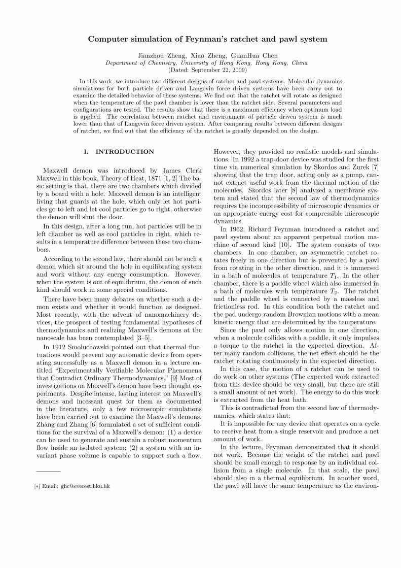
FIG. 1: An illustration of the ratchet and pawl system. Left:Top view. Right: Side view. Both chambers are filled withgas particles, a spring attached inside one end of each pawl,the ratchet in lower chamber can rotate freely

ular dynamics simulation in literature, We set up a sim-plified Feynman’s system to do molecular dynamics simu-lation. Benefited from the improvement of the computertechnology, the realistic molecular dynamics simulationsof such system can be carry out to evaluate their statis-tical behavior.

There are some research results in literature. Marcelo[35] have considered a Brownian particle in a periodic po-tential under heavy damping, and get analytical resultsby using Fokker Planck Equation. They found out thatthe Brownian particle can not get any net drift speed,even if the symmetry of the potential is broken; And ifapplied an external force with time correlations, the par-ticle can exhibit a nonzero net drift speed. Magnascoland Stolovitzky [36] later presented an analytical resultto test Feynman’s ratchet and pawl system. However, inorder to get analytical solution of Fokker Planck equa-tion, they worked in overdampped region. Astumian[37] and Bier also did similar analyze on heavily dampedBrownian particle in a periodic potential and found outthat even the net force is zero, there is a net flow. Riskenand Voigtlaender have solved the Fokker-Planck equa-tion for the extremely underdamped Brownian motion ina double-well potential[31]. Schneider and his coworkers[17] have simulated Brownian motion of non-interactingparticles in a periodic potential and driven by and exter-nal force. The Fokker-Planck equation is solved, but thepotential applied to the Brownian particle is too simpleand it is quite different from Feynman’s system.

Up to now, many researchers did similar simulationsin over damped region. However, there is no work whichconsiders underdamped region and has both ratchet andpawl setup. In our work, two models which are veryclose to Feynman’s ratchet and pawl are built for thesimulation.

3

II. FIRST MODEL

The system we have simulated contains two identicalchambers which filled with random distributed gas par-ticles. Several pawls are placed in upper chamber and aratchet consist of a simple stick and another perpendicu-lar joint stick. The angle of this two sticks are fixed. Asshowed in Figure 1. The gas molecules are hard dishesmoving inside a two-dimensional space and colliding witheach other. All collisions of gas molecules are energy- andmomentum-conserving. After particle-wall collisions, theparticle momentum reverses its component perpendicu-lar to the wall. Geometrically, the pawl, the ratchet andthe perpendicular stick are line segments of zero widthimpenetrable by the molecules (the mass of the perpen-dicular stick is zero). A spring with a force constant Kφ

is placed in one end of pawl. In the equilibrium position,the pawl angle is φ0.

The ratchet is a free rotor. It will only change its an-gular velocity during collision. The change of angularvelocity of ratchet is calculated in Appendix A. The La-grangian of the pawl can be written as

L =12

N∑

i=1

mgasv2i +

12Ipawlφ

2− 12Kφ(φ−φ0)2−Vint (1)

where vi is the velocity magnitude of the ith gas particle,φ (φ0) is the pawl angle (the equilibrium pawl angle),φ is angular velocity, Kφ is the elastic constant of thepawl spring, mgas and Ipawl are the mass of the gaseousparticles and the momentum of inertia of the pawl, re-spectively, and Vint is the interaction potential energyamong all rigid bodies in the system, which is constantexcept when particle-pawl and ratchet-pawl collisions oc-cur. The third term on the right hand side of equation de-scribes the interaction between the spring and the pawl.Equations of motion for the particle velocities and thepawl angle φ are then derived from the Lagrangian. Forinstance, in the absence of collisions, the pawl angle φ(t)follows

φ(t) = φ0 + [φ(ti)− φ0] cos

[√Kφ

Ipawl(t− ti)

]

+ φ(ti)

√Ipawl

Kφsin

[√Kφ

Ipawl(t− ti)

](2)

for t > ti, where ti denotes the starting time.As showed in Figure 24, where θ is the rotation of

the ratchet, φ (φ0) is the angle of pawl (the equilibriumangle). Kφ is the force constant. Details are explainedin Appendix A.

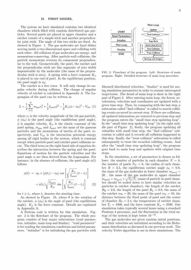
A Fortran code is written for this simulation. Fig-ure 2 is the flowchart of the program. The whole pro-gram consists of four major subroutines (read parame-ters, initialize, main loop and finalize). ”read parameter”is for reading the simulation conditions and initial param-eters. ”initialize” is for initializing the gas particles with

FIG. 2: Flowchart of the program. Left: Structure of mainprogram. Right: Detailed structure of main loop procedure

Maxwell distributed velocities. ”finalize” is used for sav-ing simulation parameters in order to resume interruptedtrajectories. The detail of main loop is show in the rightpart of Figure 2. After entering main loop, the forces, ac-celeration, velocities and coordinates are updated with agiven time step. Then, by comparing with the last step, asubroutine called ”find collision” is called to search collid-ing events occurred in current step. If there are collisions,all updated information are restored to previous step andthe program enters the ”small time step updating loop”.In the ”small time step updating loop” (in the right mid-dle part of Figure 2), firstly, the program updating allvaluables with small time step, the ”find collision” sub-routine is called and it records all collisions happened inthis step. finally, the ”treat collision” subroutine is calledsubsequently to treat the recorded colliding events. Andafter the ”small time step updating loop”, the programgoes back to main loop and updates with original timesteps.

In the simulation, a set of parameters is chosen as fol-lows: the number of particles in each chamber N = 8,the number of pawls NP = 6, the radius of each cham-ber R = 3.5, the equilibrium ratchet angle φ0 = 0.8,the mass of the gas molecules in lower chamber mgas1 =20 , the mass of the gas molecules in upper chambermgas2 = mgas1×

√T2/T1 (mass of particle in pawl cham-

ber should be scaled down to have similar velocities asparticles in ratchet chamber), the length of the ratchetRB = 2.0, the length of the pawl RL = 0.8, the mass ofthe ratchet mB = 20, the mass of the pawl mL = 10, thedistance between the fixed point of pawl and the centerof chamber RP = 2.4, the temperature of ratchet cham-ber T1 = 1000, and the force constant Kφ = 3500. Oursimulation takes typically several hours using a standardPentium 4 processor, and the fluctuation in the total en-ergy of the system is kept below 10−10.

The gas molecules are given random initial positions,and their velocities are initialized according to the Boltz-mann distribution as discussed in our previous work. Thevelocity Verlet algorithm is use in these simulations. The

4

time evolution of the system of the molecules and theratchet is simulated by adopting the following algorithm:to minimize numerical errors, adaptable time steps areused. There are two kinds of time steps in this simulation.Our program iterates a main cycle which starts from t0to the end of simulation with a time step ∆t = 0.0001.Within each cycle, the velocities and positions of all par-ticles and the trap door are updated assuming no collisiontakes place, a subroutine is then called to examine colli-sion events that may have been overlooked. Four typesof collision events are involved: particle-particle colli-sions, particle-wall collisions, particle-ratchet collisionsand particle-pawl collisions. Information of the previ-ous step is recorded so that we can restore a currentstate to the one that precedes it. The collision criteriaare: 1) particle-particle collisions: the distance betweentwo particles is less than the diameter of a particle; 2)particle-ratchet collisions(particle-pawl collisions is thesame): the distance between particle and ratchet is lessthan the radius of a particle; 3) ratchet-pawl collisions:the rotating end of ratchet cross the pawl;

We take a particle-particle collision as an example. Atthe end of each time step, the center-of-mass distancebetween two particles is measured to determine whethera collision has taken place. If there is no collision, sim-ulation carries on to the next time step. Otherwise, col-lisions need to be accounted for. In this case, the sim-ulation is restored to the recorded previous state, andthe time step is reduced to ∆t′ = 10−3dt. After therestoration, the program performs 103 steps using ∆t′.It means one regular step is divided into 103 steps ina collision event. After the collision, the simulation re-turns to the main loop with the original time step ∆t.If a three-body collision is to occur, our program recordsall the relevant information and pauses. However, sucha three-body collision event has not been encountered inour system which is composed of 16 particles with a timestep ∆t′ as small as 10−3dt.

We have carefully considered various collision eventsincluding particle-particle collisions, particle-wall colli-sions, particle-ratchet collisions, particle-pawl collisionsand ratchet-pawl collisions. Details on how these col-lision events are handled are explained in Appendix A.For a particle-wall collision, the normal component of theparticle’s velocity reverses its direction while the tangen-tial counterpart remains unchanged.

Firstly, we set no temperature difference between theratchet and pawl chamber. Figure 3 shows 1000 indi-vidual runs of this model. In these trajectories. Someof them rotate clockwise as well as some others rotatecounter clockwise.

In a individual trajectory, there are two visual pro-cesses. First, the rotor get enough energy from hot par-ticles, and cross the barrier of bending potential of theangle φ. Second, the vibrating pawl hit the rotor andthe rotor bounce back. These two processes are all dom-inated in our simulation.

Figure 4 shows the averaged results. The solid line is

FIG. 3: 1000 Individual runs of the model.

FIG. 4: Averaged rotation of the ratchet in one chamber sys-tem.

the net rotation of the rotor, and the dashed line repre-sents the standard deviation of these trajectories. Afteraveraged over 1000 individual trajectories, the net rota-tion of the ratchet is zero.

When applying lower temperature to pawl’s chamber(T2). As we expected, the averaged result of the rotorrotates clockwise as showed in Figure 5.

In individual trajectory of this case, there are also twovisual processes. First, the rotor get enough energy fromhot particles, and cross the barrier of bending potentialof the angle φ. Second, the leg of the rotor hit the pawland bounce back. After applying lower temperature tothe pawl’s chamber, the vibrations of pawl are greatlydepressed by colliding with cool particles. Therefore thefirst process becomes dominant, and the ratchet goes todesigned direction.

After fitting with a line, we can calculate the angularvelocity of the ratchet. Figure 5 shows three different

5

FIG. 5: Rotation of ratchet with different temperature con-figurations.

FIG. 6: Angular velocity of ratchet with different temperatureconfigurations.

results of the ratchet with different T1/T2. The angularvelocity become larger when higher temperature differ-ence applied.

After testing several combinations of T1/T2, as showedin Figure 6, when T1/T2 goes to 1, the ratchet has nonet rotation. Angular velocities of the ratchet increasedwhen T1/T2 become larger. When T1/T2 reaches 103,the effect of the temperature differences become smaller,hence the curve goes flat in higher difference region.

To test the efficiency of the ratchet, temperature differ-ence T1/T2 = 103 is used in later simulations. We applya constant torque against the desired rotating directionas a load applied to the ratchet. The heat flow from theratchet chamber to pawl chamber is collected by sum-marising the energy change of ratchet (or pawl) on eachratchet-pawl collision.

FIG. 7: Efficiency of the ratchet and pawl system when ap-plying different load

FIG. 8: Effect of different number of gas particle

Figure 7 shows the efficiencies of the system whendifferent loads are applied. The result shows that themaximum efficiency is 0.262% when the load is equal to1.5× 10−4. When the load exceeds 3.1× 10−4, the rotorrotates to opposite direction, hence, the efficiency goesnegative.

The number of particles included in each chamber isconsidered. Figure 8 shows that when large number ofgas particles is used, the angular velocity of the ratchetwill decrease. It is because that the rotation will be heav-ily blocked by gas particles when high density of particlesis applied.

After introducing and simulating this simplifiedratchet and pawl system, a clear picture of such sys-tem is showed. When there is no temperature differ-ence between ratchet and pawl chamber, no net rotation

6

FIG. 9: An illustration of the simplified Feynman’s ratchetand pawl system for Fokker Planck equation

will be observed. After apply lower temperature to pawlchamber, the vibrations of pawls are greatly depressed,hence the ratchet rotates as expected. Different tem-perature configurations are tested, we found out that ,in lower temperature difference region (T1/T2 < 103),higher temperature difference will result in higher ro-tating speed, and when temperature difference which islarger than 103, higher temperature difference will notaffect the angular velocity. The efficiency of the systemhas been tested. The maximum efficiency is 0.262% whenthe external load is equals to 1.5 × 10−4. External loadwhich exceeds 3.1× 10−4 will result in opposite rotationdirection of ratchet.

III. LANGEVIN SOLUTION

Langevin equation is commonly used to solve the mo-tion of Brownian particles in a potential. It is a stochasticdifferential equation. The general form of the Langevinequation for Brownian motion is as follows,

dv

dt= −γv + F (x) + Γ(t) (3)

Here, v is velocity, x is position, F (x) is the forceacted on the particle, and Γ is a Langevin force whichis a stochastic term and satisfies < Γ(t) >= 0 and< Γ(t)|Γ(t′) >= qδ(t − t′) . Here, q is correlation con-stant.

To solve this equation, one may count many individualpropagation via time t, or introduce a distribution den-sity function and solve the related Fokker Planck Equa-tion.

Figure 9 is an illustration of the simplified model ofFeynman’s ratchet and pawl system. The ratchet andpawl are both non-penetrable straight sticks with zerowidth and certain mass, mθ and mφ. The ratchet canrotate freely around the center as well as the pawl can

rotate around the fixed point with a spring attached. Theequilibrium position of the pawl is φ0. There are uncor-related Gaussian type random force on both the ratchetand the pawl.

The related Langevin equation can be written as,

ωθ = −γωθ − fθ(θ, φ, θ, φ) + Γθ(t)

θ = ωθ

ωφ = −γωφ − fφ(θ, φ, θ, φ) + Γφ(t)

φ = ωφ (4)

Here, the random forces acted on θ and φ are uncor-related and both are distributed in Gaussian type, wehave

< Γθ(t)Γθ(t′) > =2γθkTθ

Iθδ(t− t′)

< Γφ(t)Γφ(t′) > =2γφkTφ

Iφδ(t− t′)

< Γθ(t)Γφ(t′) > = 0 (5)

k is Boltzmann constant, Tθ and Tφ are the temper-ature of the ratchet and pawl chamber, γθ and γφ arefriction coefficients, and Iθ and Iφ are the momentuminertia of the ratchet and pawl respectively.

The related Fokker-Planck Equation can be written asfollows[38],

∂

∂tW (θ, φ, θ, φ, t) =

{− ∂

∂θθ +

∂

∂θ(fθ + γθ θ) + γθ

kT

Iθ

∂2

∂θ2− ∂

∂φφ

+∂

∂φ(fφ + γφφ) + γφ

kT

Iθ

∂2

∂θ2

}W (θ, φ, θ, φ, t) (6)

Here, fθ = fθ(θ, φ, θ, φ) and fφ = fφ(θ, φ, θ, φ) areforces acted on ratchet and pawl. There are sharp valuesin these functions when ratchet collides to pawl. ( Here,fθ = δθIθ and fφ = δφIφ − kφ(φ − φ0) .) Detailed def-inition of δθ and δφ are in Appendix A. Equation 4.4 isa four variable Fokker time dependent Planck Equation.There is no analytical solution [38]. To numerically solvethe equation and determine the distribution function, oneway is to use finite grid space, guess an initial distribu-tion density function and solve it by iteration. But for afour variable Fokker Planck equation, This is very timeconsuming. A easier way is to statistically solve the re-lated Langevin Equation [38] (calculate a large numberof individual trajectories), and calculate the distributionfunction of the system.

The setting in this simulation are similar to the particledriven model. The major different between them is thatthe particles in chambers are replaced by Langevin force.

7

FIG. 10: Net rotation in different T1 and T2.

Compare to the particle driven model, the correla-tion between environment and ratchet (or pawl) is muchhigher. The Langevin force is continuously acted on theratchet (or pawl), while in previous case, the gas particleonly collide on ratchet (or pawl) occasionally. Therefore,the mass of the ratchet and pawl is tuned to much smallerin order to have similar angular velocities. In our case,the mass of the ratchet and pawl are 100 times smaller.

In this simulation, to achieve similar results, a set ofparameters is chosen as follows: the number of pawlsNP = 6, the radius of each chamber R = 3.5, the equi-librium ratchet angle φ0 = 0.8, RB = 2.0, the length ofthe pawl RL = 0.8, the mass of the ratchet mB = 0.2, themass of the pawl mL = 0.1, the temperature of ratchetchamber T1 = 109, the distance between the fixed pointof pawl and the center of chamber RP = 2.4, the forceconstant Kφ = 3500, and the friction constant of theratchet and pawl are γθ = 0.5 , γφ = 5.

In order to have comparable results, the integratingtime step and total simulation time is set to ( dt = 0.0001and 500 ). Another Fortran code is written to performthis simulation. There are only ratchet-pawl collision.The structure of the program is similar to the previousone. The Langevin force is applied to the system on allmajor time steps. In later results, if not pointed out, 1000individual trajectories are counted to determine averagedproperties.

Firstly, we test the condition with no temperature dif-ference T1 = T2 = 1000. The result shows no different asin particle driven system, As the dashed line showed inFigure 10. No net rotation is observed.

When the temperature of the two chamber is set toT1 = 1000, T2 = 1. The ratcheting effect occurs, thesolid line in Figure 10 shows that there is net rotationwhen lower pawl temperature is applied.

To observe the distribution density function of the sys-tem, we have counted the distribution of angular veloc-ity of the ratchet (θ). Figure 11 is the distribution ofθ. As it shows, the central point of the distribution is

FIG. 11: Distribution of θ

FIG. 12: Angular velocity with different length of ratchet

in −0.02, the average angular velocity of ratchet is neg-ative. Therefore, the ratchet rotates to one direction asexpected.

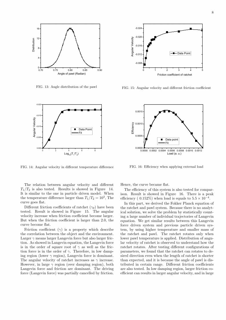
When tuning the parameter, different length of ratchet( other parameters are fixed ) is tested. Intuitively think-ing, there should be no ratcheting effect when the ratchetcannot reach the pawl which is in equilibrium position.That means, in our configuration of the device, the lengthof ratchet should larger than 1.843 in order to collide withthe pawl. However, we found out that even the ratchetis shorter than 1.843, net rotation occurs. Figure 12shows the angular velocity calculated in different lengthof ratchet. It is clear that, the ratchet rotates to desireddirection when the length is longer than 1.75. The rea-son is that the pawls are vibrating during the simulation,and there is a distribution of angle of the pawl. Figure13 is the angle distribution of the pawl in our simula-tion. It shows that the pawl have visible distribution in0.9 > φ > 0.7. This result shows that there may stillbe ratcheting effect even when the length of ratchet isshorter than expected.

8

FIG. 13: Angle distribution of the pawl

FIG. 14: Angular velocity in different temperature difference

The relation between angular velocity and differentT1/T2 is also tested. Results is showed in Figure 14.It is similar to the one in particle driven model. Whenthe temperature difference larger than T1/T2 = 103, Thecurve goes flat.

Different friction coefficients of ratchet (γθ) have beentested. Result is showed in Figure 15. The angularvelocity increase when friction coefficient become larger.But when the friction coefficient is larger than 2.0, thecurve become flat.

Friction coefficient (γ) is a property which describethe correlation between the object and the environment.Larger γ means larger Langevin force but also larger fric-tion. As showed in Langevin equation, the Langevin forceis in the order of square root of γ as well as the fric-tion force is in the order of γ. Therefore, in low damp-ing region (lower γ region), Langevin force is dominant.The angular velocity of ratchet increases as γ increase.However, in large γ region (over damping region), bothLangevin force and friction are dominant. The drivingforce (Langevin force) was partially cancelled by friction.

FIG. 15: Angular velocity and different friction coefficient

FIG. 16: Efficiency when applying external load

Hence, the curve became flat.The efficiency of this system is also tested for compar-

ison. Result is showed in Figure 16. There is a peakefficiency ( 0.152%) when load is equals to 5.5× 10−4.

In this part, we derived the Fokker Planck equation ofthe ratchet and pawl system. Because there is no analyt-ical solution, we solve the problem by statistically count-ing a large number of individual trajectories of Langevinequation. We get similar results between this Langevinforce driven system and previous particle driven sys-tem, by using higher temperature and smaller mass ofthe ratchet and pawl. The ratchet rotates only whenlower pawl temperature is applied. Distribution of angu-lar velocity of ratchet is observed to understand how theratchet rotates. After testing different configurations ofparameters, we found that the ratchet can rotates to de-sired direction even when the length of ratchet is shorterthan expected, and it is because the angle of pawl is dis-tributed in certain range. Different friction coefficientsare also tested. In low damping region, larger friction co-efficient can results in larger angular velocity, and in large

9

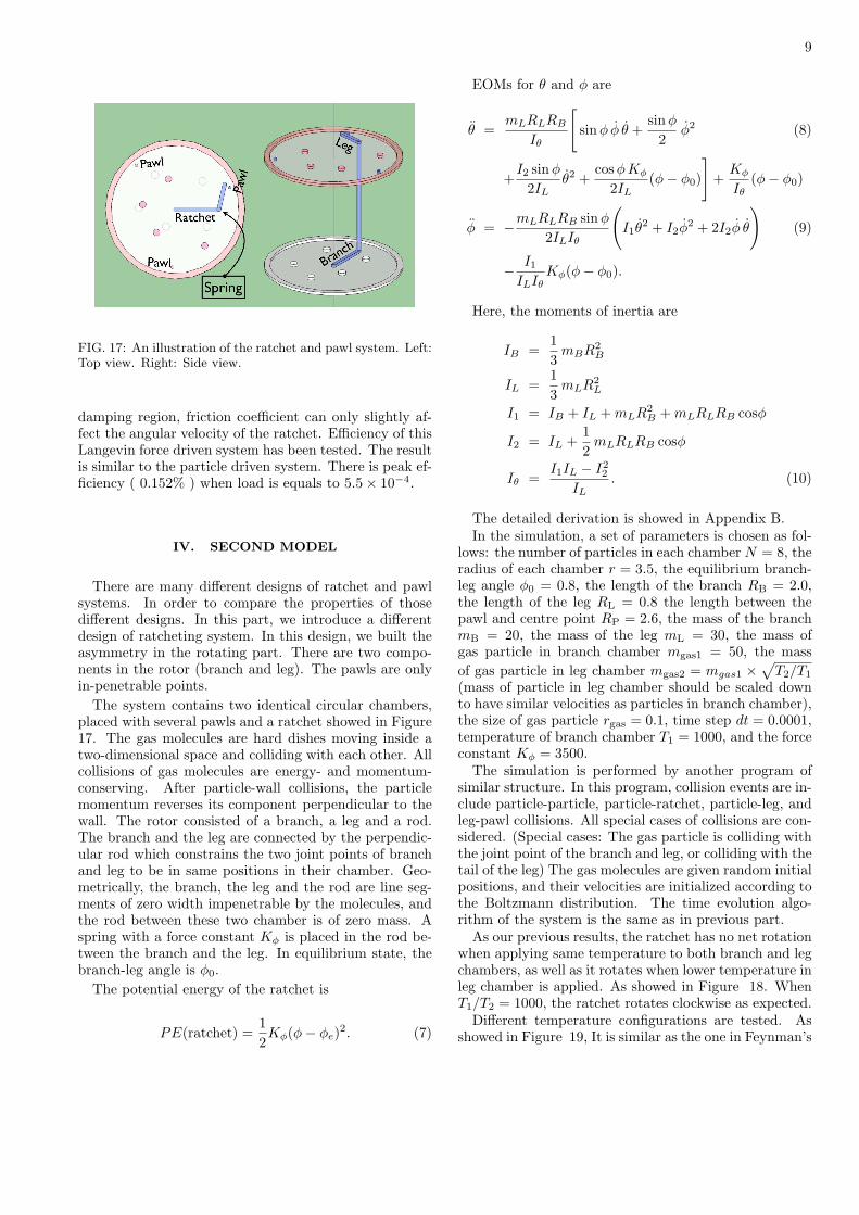
FIG. 17: An illustration of the ratchet and pawl system. Left:Top view. Right: Side view.

damping region, friction coefficient can only slightly af-fect the angular velocity of the ratchet. Efficiency of thisLangevin force driven system has been tested. The resultis similar to the particle driven system. There is peak ef-ficiency ( 0.152% ) when load is equals to 5.5× 10−4.

IV. SECOND MODEL

There are many different designs of ratchet and pawlsystems. In order to compare the properties of thosedifferent designs. In this part, we introduce a differentdesign of ratcheting system. In this design, we built theasymmetry in the rotating part. There are two compo-nents in the rotor (branch and leg). The pawls are onlyin-penetrable points.

The system contains two identical circular chambers,placed with several pawls and a ratchet showed in Figure17. The gas molecules are hard dishes moving inside atwo-dimensional space and colliding with each other. Allcollisions of gas molecules are energy- and momentum-conserving. After particle-wall collisions, the particlemomentum reverses its component perpendicular to thewall. The rotor consisted of a branch, a leg and a rod.The branch and the leg are connected by the perpendic-ular rod which constrains the two joint points of branchand leg to be in same positions in their chamber. Geo-metrically, the branch, the leg and the rod are line seg-ments of zero width impenetrable by the molecules, andthe rod between these two chamber is of zero mass. Aspring with a force constant Kφ is placed in the rod be-tween the branch and the leg. In equilibrium state, thebranch-leg angle is φ0.

The potential energy of the ratchet is

PE(ratchet) =12Kφ(φ− φe)2. (7)

EOMs for θ and φ are

θ =mLRLRB

Iθ

[sin φ φ θ +

sin φ

2φ2 (8)

+I2 sin φ

2ILθ2 +

cos φKφ

2IL(φ− φ0)

]+

Kφ

Iθ(φ− φ0)

φ = −mLRLRB sin φ

2ILIθ

(I1θ

2 + I2φ2 + 2I2φ θ

)(9)

− I1

ILIθKφ(φ− φ0).

Here, the moments of inertia are

IB =13

mBR2B

IL =13

mLR2L

I1 = IB + IL + mLR2B + mLRLRB cosφ

I2 = IL +12

mLRLRB cosφ

Iθ =I1IL − I2

2

IL. (10)

The detailed derivation is showed in Appendix B.In the simulation, a set of parameters is chosen as fol-

lows: the number of particles in each chamber N = 8, theradius of each chamber r = 3.5, the equilibrium branch-leg angle φ0 = 0.8, the length of the branch RB = 2.0,the length of the leg RL = 0.8 the length between thepawl and centre point RP = 2.6, the mass of the branchmB = 20, the mass of the leg mL = 30, the mass ofgas particle in branch chamber mgas1 = 50, the massof gas particle in leg chamber mgas2 = mgas1 ×

√T2/T1

(mass of particle in leg chamber should be scaled downto have similar velocities as particles in branch chamber),the size of gas particle rgas = 0.1, time step dt = 0.0001,temperature of branch chamber T1 = 1000, and the forceconstant Kφ = 3500.

The simulation is performed by another program ofsimilar structure. In this program, collision events are in-clude particle-particle, particle-ratchet, particle-leg, andleg-pawl collisions. All special cases of collisions are con-sidered. (Special cases: The gas particle is colliding withthe joint point of the branch and leg, or colliding with thetail of the leg) The gas molecules are given random initialpositions, and their velocities are initialized according tothe Boltzmann distribution. The time evolution algo-rithm of the system is the same as in previous part.

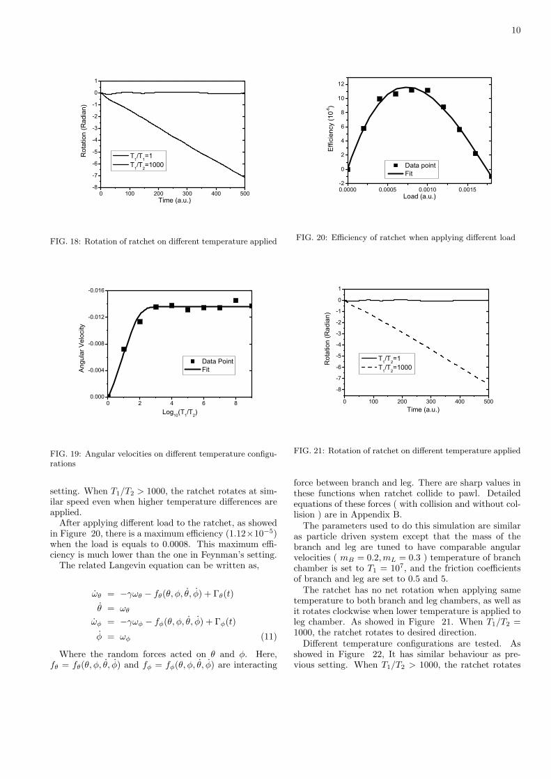
As our previous results, the ratchet has no net rotationwhen applying same temperature to both branch and legchambers, as well as it rotates when lower temperature inleg chamber is applied. As showed in Figure 18. WhenT1/T2 = 1000, the ratchet rotates clockwise as expected.

Different temperature configurations are tested. Asshowed in Figure 19, It is similar as the one in Feynman’s

10

FIG. 18: Rotation of ratchet on different temperature applied

FIG. 19: Angular velocities on different temperature configu-rations

setting. When T1/T2 > 1000, the ratchet rotates at sim-ilar speed even when higher temperature differences areapplied.

After applying different load to the ratchet, as showedin Figure 20, there is a maximum efficiency (1.12×10−5)when the load is equals to 0.0008. This maximum effi-ciency is much lower than the one in Feynman’s setting.

The related Langevin equation can be written as,

ωθ = −γωθ − fθ(θ, φ, θ, φ) + Γθ(t)

θ = ωθ

ωφ = −γωφ − fφ(θ, φ, θ, φ) + Γφ(t)

φ = ωφ (11)

Where the random forces acted on θ and φ. Here,fθ = fθ(θ, φ, θ, φ) and fφ = fφ(θ, φ, θ, φ) are interacting

FIG. 20: Efficiency of ratchet when applying different load

FIG. 21: Rotation of ratchet on different temperature applied

force between branch and leg. There are sharp values inthese functions when ratchet collide to pawl. Detailedequations of these forces ( with collision and without col-lision ) are in Appendix B.

The parameters used to do this simulation are similaras particle driven system except that the mass of thebranch and leg are tuned to have comparable angularvelocities ( mB = 0.2,mL = 0.3 ) temperature of branchchamber is set to T1 = 107, and the friction coefficientsof branch and leg are set to 0.5 and 5.

The ratchet has no net rotation when applying sametemperature to both branch and leg chambers, as well asit rotates clockwise when lower temperature is applied toleg chamber. As showed in Figure 21. When T1/T2 =1000, the ratchet rotates to desired direction.

Different temperature configurations are tested. Asshowed in Figure 22, It has similar behaviour as pre-vious setting. When T1/T2 > 1000, the ratchet rotates

11

FIG. 22: Angular velocities on different temperature configu-rations

FIG. 23: Efficiency of ratchet when applying different load

clockwise at similar speed.After applying different load to the ratchet, as showed

in Figure 23, when the load is equals to 4× 10−4, thereis a maximum efficiency (1.79× 10−5).

In this part, we have simulated another design ofratchet and pawl system, We have tested the rotatingbehavior by introducing both particle driven system andLangevin force driven system. The results from bothsystems are consistent. The ratchet rotates to designeddirection when T2 is lower than T1.

Efficiency of the system and different temperature con-figurations are tested. We found out that the efficiencyin this system is much lower then the one in Feynman’ssystem. The reason is, in Feynman’s setting, heat trans-fers from T1 to T2 only when ratchet is colliding withpawl. However, in this new design, when the rotor isrotating, the branch drags the leg around and particles

FIG. 24: For both θ and φ, the most convenient choice forrange would be (−π, π).

(or friction) in leg chamber hinder the rotation of thebranch, and hence heat transfered directly from branchto gas particles in leg’s chamber with no contribution toasymmetric rotation of the ratchet.

V. SUMMARY AND DISCUSSION

In this work, we have presented two designs of ratchetand pawl systems, and have performed molecular dy-namics simulations for both particle driven and Langevinforce driven systems to test the detailed behavior of thesesystems. We find out that the ratchet rotates as designedwhen the temperature of the pawl chamber is lower thanthe ratchet side. Several parameters and configurationshave been tested. The results show that there is a maxi-mum efficiency when optimum load applied. The correla-tion between ratchet and environment of particle-drivensystem is much lower than that of Langevin force-drivensystem. After comparing results between different de-signs of ratchet, we find out that the efficiency of theratchet is greatly depended on the design of the system.That may help us to design new nano devices in this kind.

Acknowledgments

This work was supported by the Hong Kong ResearchGrants Council (HKU 7012/04P and HKU 7127/05E)and the Committee on Research and Conference Grants(CRCG) of University of Hong Kong.

12

APPENDIX A: DETAIL OF COLLISIONS FORFEYNMAN’S RATCHET AND PAWL SYSTEM

1. Without Collision

The potential energy of the Ratchet and Pawl is dueto the spring attached to the pawl (leg).

PE(RP) =12Kφ(φ− φe)2, (A1)

where φe stands for the minimum position of the aboveparabolic potential. The moments of inertia of the legwith respect to point P and of the branch with respectto point O are

IL =13

mLR2L

IB =13

mBR2B , (A2)

respectively. The equation of motion (EOM) for φ is asfollows,

ILφ = −Kφ(φ− φe). (A3)

The exact solution for the EOM is

φ(t) = φe+(φ(t0)−φe

)cos

(√Kφ

ILt

)+φ(t0)

√IL

Kφsin

(√Kφ

ILt

),

(A4)where φ(t0) and φ(t0) are the initial displacement andvelocity for φ, respectively.

2. General formulation for collision events betweenparticles and sticks

The change of velocities for the branch, the leg and thegas molecules are denoted by δθ, δφ and δx(δy), respec-tively. Upon a single collision event, they are determinedvia the following relations,

δθ = A ∆P

δφ = B ∆P

δx = C ∆P

δy = D ∆P, (A5)

where ∆P is

∆P = −2X

Y

X = AIB θ + BILφ + CmGx + DmGy

Y = A2IB + B2IL + C2mG + D2mG

A =∂θh

IB

B =∂φh

IL

C =∂xh

mG

D =∂yh

mG. (A6)

Here h represents the distance between the particle andthe stick.

3. Ratchet hits Pawl

h = RP sin φ + RB sin(θ − φ)∂θh = RB cos(θ − φ)∂φh = RP cosφ−RB cos(θ − φ)

C = 0D = 0. (A7)

4. Gas hits Ratchet

h = x sin θ − y cos θ

∂θh = x cos θ + y sin θ

∂xh = sin θ

∂yh = − cos θ

B = 0, (A8)

where x and y are Cartesian coordinates in the systemwith

−−→OP as the positive x axis.

5. Gas hits the end of the Ratchet

This happens when the gas molecule has a finite radiusR.

h =√

(x−RB cos θ)2 + (y −RB sin θ)2 −R

∂θh =RB(x sin θ − y cos θ)

R

∂xh =x−RB cos θ

R

∂yh =y −RB sin θ

RB = 0, (A9)

13

where x and y are Cartesian coordinates in the systemwith

−−→OP as the positive x axis.

6. Gas hits Leg

h = x sin φ− y cosφ

∂φh = x cos φ + y sin φ

∂xh = sin φ

∂yh = − cos φ

A = 0, (A10)

where x and y are Cartesian coordinates in the systemwith

−−→PO as the positive x axis.

7. Gas hits the end of the Pawl

This happens when the gas molecule has a finite radiusR.

h =√

(x−RL cos φ)2 + (y −RL sin φ)2 −R

∂φh =RL(x sin φ− y cos φ)

R

∂xh =x−RL cos φ

R

∂yh =y −RL sin φ

RA = 0, (A11)

where x and y are Cartesian coordinates in the systemwith

−−→PO as the positive x axis.

8. Coordinate transformation

Assume the geometric center of a gas molecule is at(x, y) in the

−−→OX coordinate system, its coordinates in−−→

OP and−−→PO systems are (xOP , yOP ) and (xPO, yPO),

respectively. (x, y) can be transformed into (xOP , yOP )via

xOP = x cos θP + y sin θP

yOP = y cos θP − x sin θP

xOP = x cos θP + y sin θP

yOP = y cos θP − x sin θP . (A12)

(x, y) can be transformed into (xPO, yPO) via

xPO = RP − x cos θP − y sin θP

yPO = −y cos θP + x sin θP

xPO = −x cos θP − y sin θP

yPO = −y cos θP + x sin θP . (A13)

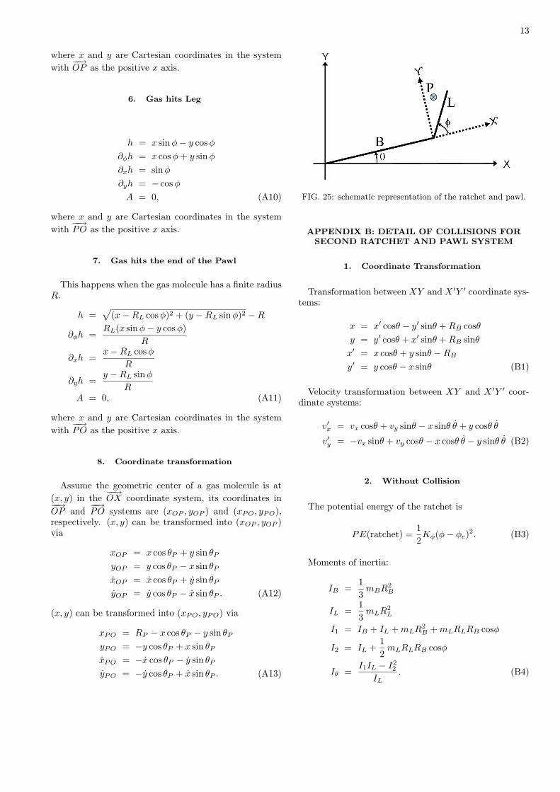
FIG. 25: schematic representation of the ratchet and pawl.

APPENDIX B: DETAIL OF COLLISIONS FORSECOND RATCHET AND PAWL SYSTEM

1. Coordinate Transformation

Transformation between XY and X ′Y ′ coordinate sys-tems:

x = x′ cosθ − y′ sinθ + RB cosθy = y′ cosθ + x′ sinθ + RB sinθ

x′ = x cosθ + y sinθ −RB

y′ = y cosθ − x sinθ (B1)

Velocity transformation between XY and X ′Y ′ coor-dinate systems:

v′x = vx cosθ + vy sinθ − x sinθ θ + y cosθ θ

v′y = −vx sinθ + vy cosθ − x cosθ θ − y sinθ θ (B2)

2. Without Collision

The potential energy of the ratchet is

PE(ratchet) =12Kφ(φ− φe)2. (B3)

Moments of inertia:

IB =13

mBR2B

IL =13

mLR2L

I1 = IB + IL + mLR2B + mLRLRB cosφ

I2 = IL +12

mLRLRB cosφ

Iθ =I1IL − I2

2

IL. (B4)

14

EOMs for θ and φ:

θ =mLRLRB

Iθ

[sin φ φ θ +

sinφ

2φ2 (B5)

+I2 sin φ

2ILθ2 +

cos φKφ

2IL(φ− φ0)

]+

Kφ

Iθ(φ− φ0)

φ = −mLRLRB sin φ

2ILIθ

(I1θ

2 + I2φ2 + 2I2φ θ

)(B6)

− I1

ILIθKφ(φ− φ0).

3. When a gas molecule hits the Branch

Before collision the velocities are vn, vt, θ and φ, re-spectively. After collision the velocities are vn, vt,

˜θ and

˜φ, respectively. Define

RG =√

x2G + y2

G

vG =√

v2n + v2

t

Cθ = −mGRG

Iθ=

mGRGIL

I22 − I1IL

Cφ =mGI2RG

IθIL=

mGRGI2

I1IL − I22

. (B7)

The change of velocity of the gas molecule perpendicularto the Branch is

δvn = vn − vn =−2Iθ(vn −RGθ)

Iθ + mGR2G

. (B8)

Therefore the velocities after the collision are

vn = δvn + vn

vt = vt

˜θ = Cθδvn + θ˜φ = Cφδvn + φ. (B9)

Transformation between vn, vt and vx, vy is

vn = vy cos θ − vx sin θ

vt = vy sin θ + vx cos θ

vn = vy cos θ − vx sin θ

vt = vy sin θ + vx cos θ

vx = −vn sin θ + vt cos θ

vy = vn cos θ + vt sin θ

vx = −vn sin θ + vt cos θ

vy = vn cos θ + vt sin θ. (B10)4. When a gas molecule hits the Leg

Before collision the velocities are vx, vy, θ and φ, re-

spectively. After collision the velocities are vx, vy,˜θ and

˜φ, respectively. Define

R′G =√

x′2G + y′2G

Dxθ =mGRBR′G cosφ (2IL −mLRLR′G)

2ILIθ(yG −RB sin θ)

Dxφ =mGR′G (I1R

′G − I2R

′G − I2RB cosφ)

ILIθ(yG −RB sin θ)

Dxy = −xG −RB cos θ

yG −RB sin θ. (B11)

The change of velocity of the gas molecule along x direc-tion is

δvx = vx − vx

=−2mG

I1D2xθ + ILD2

xφ + 2I2DxθDxφ + mGD2xy + mG

vx −

2 ×I1Dxθ θ + ILDxφφ + I2Dxθφ + I2Dxφθ + mGDxyvy

I1D2xθ + ILD2

xφ + 2I2DxθDxφ + mGD2xy + mG

.

(B12)

Therefore the velocities after the collision are

vx = δvx + vx

vy = Dxyδvx + vy

˜θ = Dxθδvx + θ˜φ = Dxφδvx + φ. (B13)

5. When the Leg hits the Pawl

Since the pawl does not move, before and after the col-lision the velocities are θ, φ and ˜

θ,˜φ, respectively. Define

Dθφ =Dxφ

Dxθ

=2I2RB cosφ− 2IBR′G − 2mLR2

BR′G −mLRLRBR′G cosφ

mLRLRBR′G cos φ− 2ILRB cos φ.

(B14)

The velocities after the collision are

˜θ =

(ILD2θφ − I1)θ − 2(ILDθφ + I2)φI1 + ILD2

θφ + 2I2Dθφ

˜φ =

(I1 − ILD2θφ)φ− 2(I1Dθφ + I2D

2θφ)θ

I1 + ILD2θφ + 2I2Dθφ

. (B15)

When φ = π2 or 3π

2 , cosφ = 0, the velocities after thecollision are

˜θ = θ˜φ = −φ− 2θ. (B16)

15

[1] J.C. Maxwell, Theory of Heat (London, 1871).[2] W. Thomson, Nature IX, 441 (1874).[3] Y. Zhao, C.C. Ma, L.H. Wang, G.H. Chen, Z.P. Xu,

Q.S. Zheng, Q. Jiang, and A.T. Chwang, Nanotechnology17, 1032 (2006);

[4] Y. Zhao, C.C. Ma, G.H. Chen, and Q. Jiang,Phys. Rev. Lett. 91, 175504 (2003)

[5] C.C. Ma, Y. Zhao, C.Y. Yam, G.H. Chen, and Q. Jiang,Nanotechnology 16, 1253 (2005).

[6] K. Zhang and K. Zhang, Phys. Rev. A 46 4598 (1992).[7] P. Skordos and W. Zurek, Am. J. Phys. 60, 876 (1992).[8] P. Skordos, Phys. Rev. E 48, 777 (1993).[9] M.v. Smoluchowski, Phys. Z. 13, 1069 (1912).

[10] R.P. Feynman, R.B. Leighton, and M. Sands, The Feyn-man Lectures on Physics I (Addison-Wesley, Reading,MA, 1963), Chap. 46.

[11] C. Jarzynski and O. Mazonka, Phys. Rev. E 59, 6448(1999).

[12] P. Meurs, C. Broeck and A. Garcia, Phys. Rev. E 70,051109 (2004).

[13] M. O. Magnasco and G. Stolovitzky, J. Stat. Phys. 93,615 (1998).

[14] C. Van den Broeck, R. Kawai, and P. Meurs, Phys. Rev.Lett. 93, 090601 (2004)

[15] C. Van den Broeck, P. Meurs, and R. Kawai, New J.Phys. 7, 10 (2005).

[16] S Velasco, J M M Roco, A Medina and A Calvo Hernan-dez J. Phys. D: Appl. Phys. 34 1000 (2001)

[17] T. Schneider, E. P. Stoll, and R. Morf, Phys. Rev. B 181417 (1978).

[18] J. Zheng, X. Zheng, Y. Zhao, etc., Phys. Rev. E 75,041109 (2007)

[19] R. B. Marcus, T. S. Ravi, T. Gmitter, Appl. Phys. Lett.56, 236 (1990).

[20] J. Sone et al., Nanotechnology 10, 135 (1999).[21] D. W. Carr, L. Sekaric, H. G. Craighead, J. Vac. Sci.

Technol. B 16, 3821 (1998).[22] D. W. Carr, S. Evoy, L. Sekaric, J. M. Parpia, H. G.

Craighead, Appl. Phys. Lett. 75, 920 (1999).[23] C. D. Montemagno, G. D. Bachand, Nanotechnology 10,

225 (1999).[24] G. D. Bachand, C. D. Montemagno, Biomed. Microde-

vices 2, 179 (2000).[25] S. M. Block, Cell 93, 5 (1998).[26] M. J. Schnitzer, S. M. Block, Nature 388, 386 (1997).[27] M. Wang et al., Science 282, 902 (1998).[28] K. Kitamura, M. Tokunaga, A. H. Iwane, T. Yanagida,

Nature 397, 129 (1999).[29] R. Yasuda, H. Noji, K. Kinosita Jr., M. Yoshida, Cell 93,

1117 (1998).[30] H. Noji, R. Yasuda, M. Yoshida, K. Kinosita Jr., Nature

386, 299 (1997).[31] H. Risken, K. Voigtlaender, J. Stat. Phys. 41, 825 (1985).[32] R.C. Tolman, The Principles of Statistical Mechanics

(Dove, New York).[33] C. Van den Broeck and R. Kawai, Phys. Rev. Lett. 96,

210601 (2006).[34] R. D. Astumian and M. Bier, Phys. Rev. Lett. 72, 1766

(1994)[35] M. Marcelo, Phys. Rev. Lett. 71, 1477 - 1481 (1993)[36] M. Marcelo and S. Gustavo, Journal of Statistical

Physics, 93 1572-9613, 1998[37] R. Astumian and M. Bier, Phys. Rev. Lett. 72, 1766 -

1769 (1994)[38] H. Risken, ”The Fokker-Planck Equation”, Springer-

Verlag Berlin Heidelberg, New York, 1989