Computationally Efficient and Robust BIC-Based Speaker Segmentation

920 IEEE TRANSACTIONS ON AUDIO, SPEECH, AND LANGUAGE PROCESSING, VOL. 16, NO. 5, JULY 2008

Computationally Efficient and RobustBIC-Based Speaker Segmentation

Margarita Kotti, Emmanouil Benetos, and Constantine Kotropoulos, Senior Member, IEEE

Abstract—An algorithm for automatic speaker segmentationbased on the Bayesian information criterion (BIC) is presented.BIC tests are not performed for every window shift, as previously,but when a speaker change is most probable to occur. This is doneby estimating the next probable change point thanks to a model ofutterance durations. It is found that the inverse Gaussian fits bestthe distribution of utterance durations. As a result, less BIC testsare needed, making the proposed system less computationallydemanding in time and memory, and considerably more efficientwith respect to missed speaker change points. A feature selectionalgorithm based on branch and bound search strategy is applied inorder to identify the most efficient features for speaker segmenta-tion. Furthermore, a new theoretical formulation of BIC is derivedby applying centering and simultaneous diagonalization. Thisformulation is considerably more computationally efficient thanthe standard BIC, when the covariance matrices are estimated byother estimators than the usual maximum-likelihood ones. Twocommonly used pairs of figures of merit are employed and theirrelationship is established. Computational efficiency is achievedthrough the speaker utterance modeling, whereas robustnessis achieved by feature selection and application of BIC tests atappropriately selected time instants. Experimental results indicatethat the proposed modifications yield a superior performancecompared to existing approaches.

Index Terms—Automatic speaker segmentation, Bayesian infor-mation criterion (BIC), speaker utterance duration distribution,inverse Gaussian distribution, simultaneous diagonalization,speech analysis.

I. INTRODUCTION

NOWADAYS, a vast rise in multimedia archives has oc-curred, partially due to the increasing number of broadcast

programs, the decreasing cost of mass storage devices, the ad-vances in compression techniques, and the wide prevalenceof personal computers. The functionality of such archiveswould be in doubt, unless data management is employed.Data management is necessary for organizing, navigating,and browsing the multimedia content, as is manifested bythe MPEG-7 standard. Here, we focus on speech. Speakersegmentation is an efficient tool for multimedia archive man-agement. It aims to find the speaker change points in an audiorecording. Speaker segmentation finds numerous applications,since it is a prerequisite for audio indexing, speaker identifica-tion/verification/tracking, automatic transcription, and dialogue

Manuscript received May 3, 2007; revised April 9, 2008. The associate editorcoordinating the review of this manuscript and approving it for publication wasProf. Gael Richard.

The authors are with the Department of Informatics, Aristotle University ofThessaloniki, Thessaloniki 54124, Greece (e-mail: [email protected];[email protected]; [email protected]).

Color versions of one or more of the figures in this paper are available onlineat http://ieeexplore.ieee.org.

Digital Object Identifier 10.1109/TASL.2008.925152

detection in movies. MPEG-7 audio low-level descriptors(e.g., AudioSpectrumProjection, AudioSpectrumEnvelope)can be used to describe efficiently a speech recording [1].In addition, MPEG-7 high-level tools, (e.g., SpokenContent)exploit speakers’ word usage or prosodic features that are alsouseful for speaker segmentation. A large number of groups andresearch centers compete for improved speaker segmentation.An example is the segmentation task administrated by the Na-tional Institute of Standards and Technology (NIST) [2]. NISThas also been working towards rich transcription evaluation(NIST/RT). Rich transcription includes speaker segmentationas a part of its diarization task [3].

A. Related Work

Extensive work in speaker segmentation has been carried outfor more than two decades. Three major categories of speakersegmentation algorithms can be found: model-based, metric-based, and hybrid ones.

In model-based segmentation, a set of models is trained fordifferent speaker classes and the incoming speech recordingis classified using the trained models. Various methods havebeen used in order to create generic models. Starting from theless complex case, a universal background model (UBM) isutilized to separate speech from nonspeech [4]. The UBM istrained by using a large volume of speech data offline. Thealgorithm can be used in real-time, because the models havebeen precalculated. Second, instead of using just one genericmodel, two universal gender models (UGM), that discriminatebetween male and female speakers can be used [5]. Third, theso-called sample speaker model (SSM) can be adopted [5]. Thisis a predetermined, generic, speaker-independent model, whichis progressively adapted into a specific speaker-dependent one.Alternatively, an anchor model can be utilized, where a speakerutterance is projected onto a subspace of reference speakers[6]. Finally, more sophisticated models can be created withthe help of hidden Markov models (HMMs) [7]–[9] or supportvector machines (SVMs) [10]. Metric-based techniques detectthe local extrema of a proper distance between neighboringwindows in order to segment an input recording. Various dis-tances have been employed. For example, a weighted squaredEuclidean distance has been used, where the weights areupdated by Fisher linear discriminant analysis [11]. Anothercriterion is the generalized likelihood ratio (GLR) test [5],[6], [9], [12], [23]. The Kullback–Leibler divergence is alsocommonly employed. It is used either in conjunction withthe Bayesian information criterion (BIC) [12], [13] or inde-pendently [14]. Alternatively, second-order statistics could beused [12]. Another closely related measure is the Hotelling

statistic, which is combined with BIC to achieve a higheraccuracy than the standard BIC for turns of short duration [15],

1558-7916/$25.00 © 2008 IEEE

KOTTI et al.: COMPUTATIONALLY EFFICIENT AND ROBUST BIC-BASED SPEAKER SEGMENTATION 921

[16]. However, the most popular criterion is BIC [7], [12], [15],[17]–[21]. Commonly used features in speaker segmentationare the Mel-frequency cepstrum coefficients (MFCCs), appliedin conjunction with BIC [1], [4], [5], [7]–[9], [11]–[13], [15],[18], [20], [22]. A milestone variant of BIC-based algorithms isDISTBIC, that utilizes distance-based presegmentation beforeapplying BIC [12]. Most recently, BIC is compared to agglom-erative clustering, minimum description length-based Gaussianmodeling, and exhaustive search. It is found that applying audioclassification into speech, noise, and music prior to speakersegmentation improves speaker segmentation accuracy [22]. Anapproach to segmentation and identification of mixed-languagespeech with BIC has been recently proposed [20]. In particular,BIC is employed to segment an input utterance into a sequenceof language-dependent segments, each of which is used then asprocessing model for mixed language identification.

Many researchers have experimented with hybrid algorithms,where first metric-based segmentation creates an initial set ofspeaker models and model-based techniques refine the segmen-tation next. In [8], HMMs are combined with BIC. In [23], an-other hybrid system is proposed, where the audio stream is re-cursively divided into two subsegments and speaker segmenta-tion is applied to both of them separately. Another interestinghybrid system is described in [9], where two systems are cou-pled, namely the LIA system and the CLIPS system. The LIAsystem is based on HMMs, while the CLIPS system is basedon BIC speaker segmentation followed by hierarchical clus-tering. The aforementioned systems are combined using dif-ferent strategies to further improve performance.

B. Proposed Approach

In this paper, an unsupervised, BIC-based system for speakersegmentation is proposed. The first contribution of the paperis in modeling the distribution of the duration of speaker ut-terances. More specifically, the next probable change point isestimated by employing the utterance duration model. In thisway, several advantages are gained, because the search is nolonger “blind” and exhaustive, as is the common case in speakersegmentation algorithms. Consequently, a considerably less de-manding algorithm in time and memory is developed. Severaldistributions have been tested as hypotheses for the distribu-tion speaker utterance durations and their parameters have beenestimated by maximum-likelihood estimation (MLE). Both thelog-likelihood criterion and the Kolmogorov–Smirnov criterionyield the inverse Gaussian (IG) distribution as the best fit. Morespecifically, distribution fitting in three datasets having substan-tially different nature verifies that IG models more accuratelythe distribution of speaker utterance duration. The first dataset,contains recorded speech of concatenated short utterances, thesecond dataset contains dialogues between actors that followspecific film grammar rules, while the last dataset contains spon-taneous speech.

The second contribution is in feature selection applied prior tosegmentation aiming to determine which MFCCs are most dis-criminative for the speaker segmentation task. The branch andbound search strategy using depth-first search and backtrackingis employed, since its performance is near optimal [24]. In thesearch strategy, the performance measure resorts to the ratio of

Fig. 1. Block diagram of the proposed approach.

the inter-class dispersion over the intra-class one. That is, thetrace of the product of the inverse within-class scatter matrixand the between-class scatter matrix is employed.

The third contribution is of theoretical nature. An alterna-tive formulation of BIC for multivariate Gaussians is derived.The new formulation is obtained by applying centering and si-multaneous diagonalization. A detailed proof can be found inAppendix I. It is shown that the new formulation is signifi-cantly less computationally demanding than the standard BIC,when covariance matrix estimators other than the sample dis-persion matrices are employed, such as the robust estimators[25], [26] or the regularized MLE [27]. In particular, simulta-neous diagonalization replaces matrix inversions and simplifiesthe quadratic forms to be computed. A detailed analysis of thecomputational cost can be found in Appendix II. The block di-agram of the proposed approach is illustrated in Fig. 1.

Experimental results are reported with respect to the twocommonly used sets of figures of merit, namely: 1) the preci-sion rate (PRC), the recall rate (RCL), and the associatedmeasure; 2) the false alarm rate (FAR) and the miss detectionrate (MDR). By utilizing both sets of figures of merit, a straight-forward comparison with other experimental results reported inrelated works is enabled. Furthermore, relationships betweenthe aforementioned figures of merit are derived. The proposedapproach yields a significant improvement in efficiency com-pared to previous approaches. Experiments were carried out ontwo datasets. The first dataset has been created by concatenatingspeakers from the TIMIT database [28]. This dataset will bereferred to as the conTIMIT test dataset. The second dataset hasbeen derived from RT-03 MDE Training Data Speech [44]. Inessence, the HUB-4 1997 English Broadcast News Speech parthas been utilized. The greatest improvement is achieved formissed speaker turn points. Compared with other approaches,the number of missed speaker change points is smaller as ex-plained in Section V. This is attributed to the fact that BIC teststake place when a speaker change is most probable to occur.

The remainder of the paper is organized as follows. InSection II, various distributions are tested for modeling theduration of speaker utterance and the IG distribution is demon-strated to be the best fit. The feature selection algorithm issketched in Section III. In Section IV, the standard BIC ispresented and its equivalent transformed BIC is derived. InSection V, the evaluation of the proposed approach is un-dertaken. Finally, conclusions are drawn in Section VI. The


derivation of the transformed BIC can be found in Appendix I,and the computational cost analysis is detailed in Appendix II.

II. MODELING THE DURATION OF SPEAKER UTTERANCES

A. Distribution of Speaker Utterance Durations

The first contribution of this paper is in modeling the distribu-tion of the duration of speaker utterances. Let us argue why sucha modeling is advantageous. By estimating the duration of aspeaker’s utterance, the search is no longer “blind.” After mod-eling, it is safe to claim that the next speaker change point mostprobably occurs after as many seconds dictated by a statistic ofspeaker utterance durations. In this context, several distributionshave been tested for a goodness-of-fit to the empirical distribu-tion of speaker utterance durations. A question that arises is whyfitting a theoretical distribution of speaker utterance durationsto the empirical one is necessary. The answer is that by doingso, distribution parameters take into account the structure of thedata. Moreover, finding such a theoretical distribution is inter-esting per se and this result may find additional applications,e.g., in speech synthesis.

The following distributions have been considered: Birn-baum–Saunders, Exponential, Extreme value, Gamma, IG,Log-logistic, Logistic, Lognormal, Nakagami, Normal,Rayleigh, Rician, t-location scale, and Weibull. MLE hasbeen used to calculate the best fitting parameters of eachdistribution. Here, the parameters under consideration are themean and the variance. In order to evaluate the goodness-of-fit,the log-likelihood and the Kolmogorov–Smirnov criteria havebeen computed.

The TIMIT database was used first in order to model theduration of speaker utterances. The TIMIT database includes6300 sentences uttered by 630 speakers, both male and femaleones, who speak various U.S. English dialects. The recordingsare mono-channel, the sampling frequency is 16 KHz, andthe audio PCM samples are quantized in 16 bits [28]. In total,55 recordings of artificially created dialogues along with theground-truth associated with speaker changes comprise theconTIMIT dataset.1 The recordings have a total duration ofabout 1 h. Since a transition between speech and silence is notsimilar to a transition between two speakers, the inter-speakersilences have been reduced so that conversations sound like real[12]. Thus, each segment of a speaker is followed by a segmentof another speaker. This is equivalent to silence removal, whichis a common preprocessing step [4], [8], [13], [15]. 935 speakerchange points occur in the conTIMIT dataset. Throughout theconTIMIT dataset, the minimum duration of an utterance is1.139 s and the maximum one is 11.751 s, while the meanduration is 3.286 s with a standard deviation equal to 1.503 s.Ten out of the 55 recordings of the conTIMIT dataset, randomlychosen, were used to create the conTIMIT training-1 dataset,employed in modeling the speaker utterance duration.

IG distribution has been found to be the best fit with re-spect to both log-likelihood and Kolmogorov–Smirnov test. Thevalues of mean utterance duration and standard deviation for theconTIMIT training-1 dataset under the IG model equal 3.286s and 1.388 s, respectively. An illustration of the best fit for

1conTIMIT dataset is available at http://poseidon.csd.auth.gr/LAB_RE-SEARCH/Latest/data/conTIMIT dataset.zip

the aforementioned distributions to the empirical distributionof speaker utterance durations can be seen in Fig. 2 with re-spect to the probability-probability (P-P) plots. Let us denotethe mean and the standard deviation of durations by and .Let be the th normalized theoretical cumulative den-sity function (cdf) tested. To make a P-P plot, uniform quantiles

, are defined in the horizontalaxis, where is the number of the samples whose distributionis estimated. The vertical axis represents the value admitted bythe theoretical cdf at , i.e., , where

is the th-order statistic of utterance durations. That is, thedurations are arranged in an increasing order and the th sortedvalue is chosen. The better the theoretical cdf approximates theempirical one, the closer the points are tothe diagonal [29].

To validate that IG distribution generally fits best the empir-ical speaker utterance duration distribution, another dataset hasbeen employed, to be referred to as the movie dataset [30]. Inthis dataset, 25 audio recordings are included that have been ex-tracted from six movies of different genres, namely: AnalyzeThat, Cold Mountain, Jackie Brown, Lord of the Rings I, Pla-toon, and Secret Window. Indeed, Analyze That is a comedy,Platoon is an action movie, and Cold Mountain is a drama. Thus,dialogues of different natures are included in the movie dataset.Speaker segmentation has been performed by human agents.Having the ground-truth speaker change points, the distributionof speaker utterance duration for the movie dataset is modeledby applying the same procedure as for the conTIMIT training-1dataset. The best fit is found to be the IG distribution, once again,with respect to both log-likelihood and Kolmogorov–Smirnovtest. This outcome is of great importance, since the dialoguesare not recorded in a clean environment. Longer pauses or over-laps between the actor utterances exist and background music ornoise occurs. However, as expected, different parameters fromthose estimated in the conTIMIT training-1 dataset are obtained.In the movie dataset, the mean duration equals 5.333 s, while thestandard deviation is 6.189 s. Accordingly, modeling the dura-tion of speaker utterances by an IG distribution helps to predictthe next speaker change point.

B. Mathematical Properties of the IG Distribution and itsApplication

Some of the main mathematical properties of the IG distri-bution are briefly discussed next. The IG distribution, or Walddistribution, has probability density function (pdf) with param-eters and [31], [32]

(1)

where . The IG probability density is always posi-tively skewed. Kurtosis is positive as well. For realizations,

of an IG random variable the MLEs of and

are: , where

and . Obviously, does not coincidewith the sample dispersion. One of the most important proper-ties of the IG distribution is its infinite divisibility, which impliesthat the IG distribution generates a class of increasing Lèvi pro-cesses [33]. Lèvi processes contain both “small jumps” and “big


Fig. 2. (a) P-P plots for distributions Birnbaum–Saunders, Exponential, Extreme value, Gamma for the conTIMIT training-1 dataset. (b) P-P plots for distributionsIG, Log-Logistic, Logistic for the conTIMIT training-1 dataset. (c) P-P plots for distributions Lognormal, Nakagami, Normal, Reyleigh for the conTIMIT training-1dataset. (d) P-P plots for distributions Rician, t-location scale, Weibull for the conTIMIT training-1 dataset.

jumps.” Such jumps are Poisson point processes that are com-monly used to model the arrival time of an event. In the caseunder consideration, the arrival time refers to a speaker changepoint. This property makes Lèvi processes candidates for mod-eling the speaker utterance duration. “Small jumps” occur ifthere are lively exchanges (stichomythia) and “big jumps” occurfor monologues.

In conclusion, modeling the speaker utterance duration en-ables us to perform BIC tests when a speaker change point ismost probable to occur. The simplest approach is to assume thata probable speaker change point occurs every seconds, where

is a submultiple of the expected duration of speaker utterances.should be chosen at the same order of magnitude as the sample

dispersion. This technical solution does not exclude other alter-natives, such as setting to a submultiple of the mode of (1) that

is given by [34].If the total length of the audio recording is , then

BIC tests take place. In straightforward implementation ofBIC-based speaker segmentation, BIC tests areperformed, where is the window shift of several milliseconds.Thus, % less BIC tests are performed by takinginto account the duration of utterances, when compared to the

straightforward implementation of BIC-based speaker segmen-tation. If a probable change point is not confirmed throughthe BIC test, the information contained in the last secondsupdates the existing speaker model. The use of a submultipleof the expected speaker utterance duration enables us to reducethe probability of missed speaker change points, as explained inSection V. Previous experiment demonstrates that under-seg-mentation, caused by a high number of miss detections, ismore cumbersome to remedy than over-segmentation causedby a high number of false alarms [12], [13], [15], [16], [23],[40]. For example, over-segmentation could be alleviated byclustering and/or merging. The use of within the context ofBIC is described in Section IV.

III. FEATURE EXTRACTION AND SELECTION

Different features yield a varying performance level inspeaker segmentation applications [13]. This fact motivated theauthors to invest in feature selection for speaker segmentation,which is the second contribution of the paper.

MFCCs, sometimes with their first-order (delta) and/orsecond-order differences (delta-delta) are the most commonlyused features in speaker segmentation. Furthermore, MFCCs


TABLE ISELECTED 24 MFCCS FOR THE CONTIMIT TRAINING-2 DATASET

were used in various techniques besides BIC such as HMMs[9] or SVMs [10]. Still, not all the researchers employ thesame MFCC order in BIC-based approaches. For example, 24MFCCs are employed in [7], while 12 MFCCs and their firstdifferences are utilized in [12] and [20]. Thirty-two MFCCs areused in [11]. In [4], 16 MFCCs are applied, while 12 MFCCsalong with their delta and delta-delta coefficients are employedin [9]. Twenty-three MFCCs are utilized in [1] and [8] and24 MFCCs are applied in [5], [15], and [18]. A more detailedstudy is presented in [22], where a comparative study between12 MFCCs, 13 MFCCs and their delta coefficients, and 13MFCCs, their delta, and delta-delta coefficients is performed.

A different approach is investigated here. Instead of tryingto reveal the MFCC order that yields the most accurate speakerturn point detection results, an effort is made to find out anMFCC subset that is more suitable for detecting a speakerchange. The MFCCs are calculated every 10 ms with 62.5%overlap by the algorithm described in [35]. An initial set con-sisting of 36 MFCCs is formed and the goal is to derive thesubset, which contains the 24 more suitable MFCCs for speakersegmentation, since utilizing 24 coefficients is commonplacein [5], [15], and [18].

Let us test the hypothesis that there is a speaker change pointagainst the hypothesis that there is no speaker change point.Speakers change once under the first hypothesis, while a mono-logue is observed under the second one. For training purposes,an additional dataset of 50 recordings was created from speakerutterances derived in the TIMIT database, referred to as theconTIMIT training-2 dataset, that is disjoint to the conTIMITdataset.2 Twenty-five out of the 50 recordings contain a speakerchange point and the remaining 25 recordings do not. In thisway, two classes are presumed: the first class represents aspeaker change and includes 25 recordings with one speakerchange and the second class corresponds to no speaker changesand includes 25 recordings with monologues. We assume thatthe mean feature vectors in the two different classes are dif-ferent in order to enable discrimination [24]. The goal of featureselection is to find a feature subset of dimension . Inour case, . Let denote the performance measure. Fea-ture selection finds such that ,where and is the number of distin-guishable subsets containing elements. If 24 out of the 36

coefficients are to be selected, then is enormous.

As a result, a more efficient search strategy than exhaustivesearch is required. Such an alternative is branch and bound,which attains an almost optimal performance [24]. The searchprocess is accomplished systematically by means of a treestructure consisting of levels. A level is

2conTIMIT training-2 dataset is available at http://poseidon.csd.auth.gr/LAB_RESEARCH/Latest/data/conTIMIT training-2 dataset.zip

composed of a number of nodes, and each node corresponds toa coefficient subset. At the highest level, there is only one nodecorresponding to the full set of coefficients. At the lowest level,there are nodes containing 24 coefficients. The search processstarts from the highest level by systematically traversing alllevels until the lowest level is reached. The traversing algorithmuses depth-first search with a backtracking mechanism. Thismeans that if is the best performance found so far, thenbranches whose performance is worse than are skipped [24].

The selection criterion can be defined in terms of scattermatrices. A scatter matrix gives information about the disper-sion of samples around their mean. The within-class scatter ma-trix describes the within-class dispersion. The between-classscatter matrix describes the dispersion of the class-dependentsample means around the gross mean. Mathematically, is de-fined by

(2)

where stands for the matrix trace operator. , as definedin (2), is a monotonically increasing function of the distance be-tween the mean vectors and a monotonically decreasing func-tion of the scattering around the mean vectors. Moreover, (2)is invariant to reversible linear transformations. In addition, itis ideal for Gaussian distributed feature vectors. To a first ap-proximation, MFCCs are assumed to follow the Gaussian dis-tribution. Under this assumption, (2) guarantees the best perfor-mance [24].

From each recording, 36-order MFCCs are extracted. Theselected 24 MFCCs for the conTIMIT training-2 dataset canbe seen in Table I. Although the selection of MFCCs, as inTable I, might depend on the dataset used for feature selec-tion, the aforementioned feature selection can be applied to anydataset. MFCCs shown in Table I are used in conjunction withtheir delta and delta-delta coefficients, in order to capture theirtemporal evolution that carries additional useful information. Ingeneral, the temporal evolution is found to increase efficiency[9], [15], [20], [22]. However, in [12], it is reported that usingdelta and delta-delta coefficients impairs efficiency.

Alternatively, one could replace (2) with BIC (5) itself. Thenfeature selection is performed by a wrapper instead of a filter[36], as (2) implies. In such case, the selected MFCCs are:1st–18th, 22nd, 23rd, 27th, 28th, 31st, and 35th. The computa-tion time required by (2) is less by 187.06% than that requiredby BIC, when a PC with a 3-GHz Athlon processor and 1 GBof RAM is used. In Section V, we comment on the accuracy ofthe latter feature selection method.

IV. BIC-BASED SPEAKER SEGMENTATION

In this section, the BIC criterion is detailed, and an equivalentBIC criterion is derived that is considerably less computation-


ally demanding. It is also explained how the contributions ofSections II and III are utilized in conjunction with BIC.

BIC is a maximum-likelihood, asymptotically optimal,Bayesian model selection criterion penalized by the modelcomplexity. For speaker turn detection, two different modelsare employed. Assume that there are two neighboring chunks

and around time . The problem is to decide whether ornot a speaker change point exists at . Let and

, be the numbers of samples in chunks , and, respectively. Obviously, . The problem is

formulated as a two hypothesis testing problem.Under there is no speaker change point at time . MLE

is used to compute the parameters of a Gaussian distributionthat models the data samples in . Let us denote by theparameters of the Gaussian distribution, i.e., the mean vector

and the full covariance matrix . The log-likelihoodunder is

(3)

where which are assumed to beindependent. consists of the 24 selected MFCCs with theirdelta and delta-delta coefficients, i.e., . Under thereis a speaker change point at time . The chunks and aremodeled by distinct multivariate Gaussian densities, whose pa-rameters are denoted by and , respectively. Their defini-tion is similar to . The log-likelihood under is givenby

(4)

The BIC is defined as

(5)

where is a data-dependent penalty factor (ideally 1.0). If, then time is considered to be a speaker change point.

Otherwise, there is no speaker change point at time . Thestandard BIC formulation for multivariate Gaussian densities

can be analytically written as

(6)

where is defined as

(7)

In the light of the discussion made in Section II, BIC tests areperformed every seconds, where is a submultiple of the ex-pected duration of speaker utterances. The window size is alsoset equal to taking into consideration as many data as possible.When more data are available, more accurate Gaussian modelsare built, since BIC behaves better for large windows, whereasshort changes are not easily detectable by BIC [12], [16]. More-over, it was shown in [22], that the bigger the window size, thebetter the performance.

Next, a novel formulation of the BIC is theoretically derived.It is assumed that , and are full covariance matrices.Moreover, the covariance matrix estimators are not limited tosample dispersion matrices for which BIC defined in (6)–(7)obtains the simplified form (21), as explained in Appendix I.For example, one may employ the robust estimators of covari-ance matrices [25], [26] or the regularized MLEs [27]. To obtainthe novel formulation, we apply first centering and then simulta-neous diagonalization for the pairs of and . Letus define the mean vector in chunk as . The centering trans-formation is . Next, simultaneous diagonalizationof and is applied. Let be the diagonal matrix of theeigenvalues of and be the corresponding modal matrix.Let us define ,where is the diagonal matrix of eigenvalues of , andis the corresponding modal matrix. The simultaneous diagonal-ization transformation yields for

(8)

Let and . Fol-lowing the same strategy, we obtain for

(9)

In Appendix I, it is shown that (6) is equivalently rewritten as

(10)

where is an appropriate threshold derived analytically in (26).Concerning the computational cost, simultaneous diagonal-

ization replaces matrix inversions and simplifies the quadraticforms to be computed. This leads to a substantially less com-putational costly transformed BIC, as opposed to the standardBIC. As it is detailed in Appendix II, the computational cost ofthe standard BIC in flops, excluding the cost of , is

(11)

whereas the computational cost of the transformed BIC, ex-cluding the cost of , equals

(12)

Since , by comparing (11) and (12), it can be seenthat the standard BIC is more computationally costly than itstransformed alternative.

To sum up, the algorithm can be roughly sketched as follows.1) Initialize the interval to and let .2) Until the audio recording end, use BIC with the selected

MFCCs to evaluate if there is a change point in .


TABLE IIPERFORMANCE OF BIC ON THE CONTIMIT TEST DATASET

WITHOUT MODELING THE SPEAKER UTTERANCE DURATION

NOR APPLYING FEATURE SELECTION

3) If there is no speaker change point in , then .Go to step 2).

4) If there is a speaker change point in , then. Go to step 2).

It is reminded that is a submultiple of the mean utteranceduration, which is obtained by the analysis in Section II and theterm selected MFCCs refers to the MFCCs chosen by the featureselection algorithm, described in Section III.

V. EXPERIMENTAL RESULTS AND DISCUSSION

A. Figures of Merit

To judge the efficiency of speaker turn point detection algo-rithms, two sets of figures of merit are commonly used. On theone hand, one may use the false alarm rate (FAR) and the missdetection rate (MDR) defined as

FARFA

GT FA

MDRMDGT

(13)

where FA denotes the number of false alarms, MD the number ofmiss detections, and GT stands for the number of actual speakerturns, i.e., the ground truth. A false alarm occurs when a speakerturn is detected although it does not exist, while a miss detectionoccurs when the process does not detect an existing speaker turn[12], [23]. On the other hand, one may employ the precision(PRC), recall (RCL) and rates given by

PRCCFCDET

CFCCFC FA

RCLCFCGT

CFCCFC MD

PRC RCLPRC RCL

(14)

where CFC denotes the number of correctly found changes andDET CFC FA is the number of detected speaker changes.

admits a value between 0 and 1. The higher its value is,the better performance is obtained [8], [18]. Between the pairsFAR MDR and PRC RCL , the following relationships

hold:

MDR RCL FARRCL FA

DET PRC RCL FA(15)

In order to facilitate a comparative assessment of our resultswith others reported in the literature, the evaluation of the pro-posed approach is carried out using all the aforementioned fig-ures of merit.

TABLE IIIPERFORMANCE OF BIC ON THE CONTIMIT TEST DATASET

WITH MODELING THE SPEAKER UTTERANCE DURATION

TABLE IVPERFORMANCE OF BIC ON THE CONTIMIT TEST

DATASET WITH FEATURE SELECTION

TABLE VPERFORMANCE OF THE PROPOSED SYSTEM ON THE CONTIMIT TEST

DATASET SYSTEM (WITH MODELING THE SPEAKER UTTERANCE

DURATION AND FEATURE SELECTION)

B. Evaluation

1) Comparative Performance Evaluation on the conTIMITTest Dataset: The total number of recordings in the conTIMITdataset is 55. The evaluation is performed upon 49 randomlyselected recordings of the conTIMIT dataset, forming the con-TIMIT test dataset. The remaining six were used to determinethe value of the BIC penalty-factor and to create the conTIMITtraining-3 dataset. Although the conTIMIT dataset is an artifi-cially created dataset and includes no real conversations, per-formance assessment over the conTIMIT test dataset is still in-formative. It is also reminded that ten randomly chosen record-ings out of the 55 ones of the conTIMIT dataset, are employedto model the speaker utterance duration (conTIMIT training-1dataset). Consequently, there is a partial overlap between theconTIMIT test dataset and the conTIMIT training-1 dataset. Ithas been reported that BIC performance is likely to reach a limit[20]. There are four reasons for that: 1) estimates of the BICmodel parameters are used, 2) the penalty-factor may not betuned properly, 3) the data are assumed to be jointly normal,but this is an assumption, frequently not validated, for examplewhen voiced speech is embedded into noise [37], and 4) re-searchers have found that BIC faces problems for small samplesets [37], [38]. Researchers tend to agree that BIC performancedeteriorates when a speaker utterance does not have sufficientduration, which should be more than about 2 s. For the con-TIMIT test dataset, the tolerance equals 1 s. That is, 0.5 s beforeand after the actual speaker change point.

For evaluation purposes, four systems are assessed, namely:1) The BIC system without speaker utterance duration estima-tion and feature selection. This is the baseline system (system 1).2) The BIC system with speaker utterance duration estimation(system 2). 3) The BIC system with feature selection (system3). 4) The proposed system, that is the BIC system with speakerutterance duration estimation and feature selection (system 4).The window shift is set equal to the half of the average speaker


TABLE VIF-STATISTIC VALUES AND P-VALUES FOR PRC, RCL, F , FAR, AND MDR OF THE FOUR SYSTEMS TESTED ON THE CONTIMIT TEST DATASET

utterance duration for systems 2 and 4, whereas is equal to 0.2s for systems 1 and 3.

BIC performance on the conTIMIT test dataset without mod-eling the speaker utterance duration and feature selection is de-picted in Table II. The performance of BIC with modeling thedistribution of the speaker utterance is exhibited in Table III,while its performance when feature selection is applied only issummarized in Table IV. The overall performance of the pro-posed system (system 4) is summarized in Table V. For all sys-tems, the figures of merit are computed for each audio recording,and then their corresponding mean value and standard deviationare reported [43]. Concerning system 4, if (2) is replaced byBIC, it is found that PRC RCLFAR , and MDR . However, it is reminded thatthe improvement is achieved at the cost of constraining the gen-eralization ability.

Our aim is to validate that each system differentiates signif-icantly from the others concerning their mean figures of merit.First, one-way analysis of variance (one-way ANOVA) is ap-plied. The null hypothesis tested is that the four system mean fig-ures of merit are equal. The alternative hypothesis states that thedifferences among the figures of merit are not due to random er-rors, but due to variation among unequal mean figures of merit.That is, the null hypothesis declares that the systems do not dif-ferentiate significantly from one another, while the alternativehypothesis suggests that at least one of the systems differs fromthe remaining. The F-statistic value and its p-value for all fiveefficiency measures are indicated in Table VI. From Table VI,it is evident that the four systems are statistically different, withrespect to PRC, RCL, , and MDR, whereas there appears tobe no significant difference with respect to the FAR at 95% con-fidence level.

One-way ANOVA assures us that at least one system is dif-ferent from the others. However, no information is providedabout the pairs of systems that differentiate. Tukey’s method orhonestly significant difference method is applied to find the pairsof systems that differentiate [39]. Tukey’s method is designedto make all pairwise comparisons of means, while maintainingthe confidence level at a predefined level. Moreover, it is op-timal for balanced one-way ANOVA, which is our scenario. For

systems, there are possible combinations (e.g.,six possible combinations are examined for ). Tukey’smethod for the same number of measurements is applied, i.e.,49. The critical test statistic is obtained from the Studentizedrange statistic.

Since one-way ANOVA has validated that FAR differencesare not significant, Tukey’s method is applied to the remainingfigures of merit, i.e., PRC RCL , and MDR for the same con-fidence level 95%. The corresponding confidence intervals forall pairwise comparisons among the four systems for the afore-mentioned figures of merit can be seen in Tables VII–X, respec-tively. If the confidence interval includes zero, the difference isnot significant. It is clear from Tables VII–X that zero is not

TABLE VII95% CONFIDENCE INTERVALS FOR ALL PAIRWISE COMPARISONS

OF THE FOUR SYSTEMS FOR PRC

TABLE VIII95% CONFIDENCE INTERVALS FOR ALL PAIRWISE COMPARISONS

OF THE FOUR SYSTEMS FOR RCL

TABLE IX95% CONFIDENCE INTERVALS FOR ALL PAIRWISE COMPARISONS

OF THE FOUR SYSTEMS FOR F

TABLE X95% CONFIDENCE INTERVALS FOR ALL PAIRWISE COMPARISONS

OF THE FOUR SYSTEMS FOR MDR

included in any interval. Thus, for any pairwise system compar-ison and any figure of merit from PRC RCL , and MDR thedifference is significant.

Accordingly, there is statistical evidence that both speakerutterance modeling and feature selection improve performancesignificantly either individually or combined for PRC RCL, ,and MDR. This is not the case for FAR.

2) MDR Histogram of the conTIMIT Test Dataset: We focuson the results of the proposed system for the conTIMIT testdataset depicted in Table V. The MDR histogram is plotted inFig. 3. A clear peak exists near to 0, which is the ideal case. The


Fig. 3. Histogram of MDR in the conTIMIT test dataset.

TABLE XICORRELATION COEFFICIENT BETWEEN THE PAIRS OF FIGURES

OF MERIT FOR THE CONTIMIT TEST DATASET

latter is a direct outcome of the fact that two-hypothesis BICtests are carried out at times, where a speaker change point ismost probable to occur.

3) Correlation Among Figures of Merit on the conTIMITTest Dataset: The correlation coefficient between the figures ofmerit for the conTIMIT test dataset can be seen in Table XI. Thecorrelation coefficient between RCL and MDR is , as a con-sequence of (15). The pairs: 1) (PRC, RCL) and (PRC, MDR);2) RCL and MDR ; 3) (FAR, RCL) and (FAR, MDR)have opposite signs. That is, when the first quantity increases,the second decreases and vice versa. The degree of linear depen-dence is indicated by the absolute value of the correlation index.It is seen that (PRC, and (PRC, FAR) exhibit the strongestcorrelation.

4) Performance Evaluation on the HUB-4 1997 EnglishBroadcast News Speech Dataset: Aiming to verify the effi-ciency of the proposed contributions, i.e., modeling the speakerutterance duration and feature selection on real data, RT-03MDE Training Data Speech is utilized [44]. To facilitateperformance comparisons between the proposed system andother systems, we confine ourselves to broadcast news audiorecordings, that is the HUB-4 1997 English Broadcast NewsSpeech dataset [41]. The recordings are mono-channel, thesampling frequency is 16 KHz, and the audio PCM samplesare quantized in 16 bits. The selected audio recordings have aduration of approximately 1 h.

20% of the selected audio recordings are used for estimatingthe speaker utterance duration distribution. For the third time,IG distribution is verified to be the best fit for modeling

speaker utterance duration by both the log-likelihood and theKolmogorov–Smirnov criteria. In this case, the mean durationequals 23.541 s and the standard deviation equals 24.210 s.Since the standard deviation value is considerably large, isset equal to one eighth of the mean speaker utterance duration.This rather small submultiple aims to reduce the probabilityof missing a speaker change for the reasons explained inSection II-B.

To assess the robustness of the MFCCs shown in Table I,the same coefficients along with their corresponding delta anddelta-delta coefficients have been used in the HUB-4 1997 Eng-lish Broadcast News Speech dataset. The proposed algorithm istested on the remaining 80% of the selected audio recordings.For the HUB-4 1997 English Broadcast News Speech dataset,since the dialogues are real, the tolerance should be greater, as isexplained in [12]. Motivated by [23], that also employs broad-casts, the tolerance is equal to 2 s. The achieved figures of meritare: PRC RCL FAR ,and MDR .

5) Performance Discussion: Before discussing the perfor-mance of the proposed system with respect to other systems,let us argue why it is generally a good choice to minimize MDeven if FA is high [12]. FA can be more easily removed [13],[15], [16], [40], for example through clustering. PRC and FARare associated with FA, while RCL and MDR depend on MD.This means that PRC and FAR are less cumbersome to remedythan RCL and MDR.

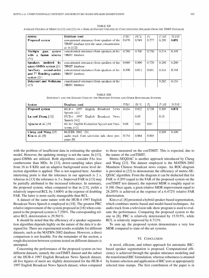
The proposed system is evaluated on the conTIMIT testdataset first. It outperforms three other systems tested on asimilar dataset, created by concatenating speakers from theTIMIT database, as described in [21]. Although the dataset in[21] is substantially smaller than the conTIMIT test dataset,the nature of the audio recordings is the same enabling usto conduct fair comparisons. The performance achieved bythe previous approaches is summarized in Table XII. Missingentries are due to the fact that not all researchers use the sameset of figures of merit, which creates further implications indirect comparisons. PRC and FAR of the proposed system onthe conTIMIT test dataset are slightly deteriorated than thoseobtained by the multiple pass system with a fusion schemewhen speakers are modeled by quasi-GMM systems. However,RCL and MDR are substantially improved. RCL and MDRare also improved with respect to the two remaining systems.Finally, the superiority of the proposed system against the threesystems developed in [21] is demonstrated by the fact thatits value is relatively improved by 7.917%, 6.438%, and28.007%, respectively. In [12], the used dataset was createdby concatenating speaker utterances from the TIMIT database,too. However, this concatenation is not the same to the oneemployed here. Although FAR is slightly better that ours, thereported MDR for the proposed system is considerably lower.The relative MDR improvement equals 67.308%.

The proposed system is also assessed on the HUB-4 1997English Broadcast News Speech dataset. As is demonstratedin Table XIII, the same dataset is utilized in [13]. The systempresented in [13] is a two-step system. The first step is a“coarse-to-refine” step, whereas the second step is a refinementone that aims at reducing FAR. Both our algorithm and theone in [13] apply incremental speaker model updating to deal


TABLE XIIAVERAGE FIGURES OF MERIT IN [12] AND [21] ON A SIMILAR DATASET CREATED BY CONCATENATING SPEAKERS FROM THE TIMIT DATABASE

TABLE XIIIEFFICIENCY AND THE DATASET USED BY THE PROPOSED SYSTEM AND OTHER BENCHMARK SYSTEMS

with the problem of insufficient data in estimating the speakermodel. However, the updating strategy is not the same. In [13],quasi-GMMs are utilized. Both algorithms consider FAs lesscumbersome than MDs. In [13], down-sampling takes placefrom 16 to 8 KHz and an adaptive background noise level de-tection algorithm is applied. This is not required here. Anotherinteresting point is that the tolerance in our approach is 2 s,whereas in [13] the tolerance is 3 s. Improved FAR in [13] maybe partially attributed to the increased tolerance. In summary,the proposed system, when compared to that in [13], yields arelatively improved RCL by 3.600% at the expense of doublingFAR. The latter is more easily manageable than RCL.

A dataset of the same nature with the HUB-4 1997 EnglishBroadcast News Speech is employed in [18]. The greatest PRCrelative improvement of the system proposed in [18] when com-pared to the proposed system is 7.256%. The corresponding rel-ative RCL deterioration is 29.501%.

It should be noted that the efficiency of a speaker segmenta-tion algorithm depends highly on the nature of the data it is de-signed for. There are experimental results available for differentdatasets, such as the MATBN-2002 database. However, a directcomparison is not feasible. For the remainder of the section, arough discussion between systems tested on different datasets isattempted.

Concerning the performance of the proposed system on twodifferent datasets, namely the conTIMIT dataset and the subsetof the HUB-4 1997 English Broadcast News Speech dataset,all five figures of merit are slightly deteriorated for the HUB-41997 English Broadcast News Speech dataset, when compared

to those measured on the conTIMIT. This is expected, due tothe nature of the conTIMIT.

Metric-SEQDAC is another approach introduced by Chengand Wang [23]. The dataset employed is the MATBN-2002Mandarin Chinese broadcast news corpus. An ROC-diagramis provided in [23] to demonstrate the efficiency of metric-SE-QDAC algorithm. From the diagram it can be deducted that forFAR (equal to the FAR of the proposed system on theconTIMIT test dataset), the reported MDR is roughly equal to0.100. Once again, a great relative MDR improvement equal to28.205% is achieved at the expense of a 6.472% relative FARdeterioration.

Kim et al. [8] presented a hybrid speaker-based segmentation,which combines metric-based and model-based techniques. Anaudio track from a television talk show program is used to eval-uate the performance. Comparing the proposed system to theone in [8], PRC is relatively deteriorated by 15.915%, whileRCL is relatively improved by 6.713%.

To sum up, the proposed system demonstrates a very lowMDR compared to state-of-the-art systems.

VI. CONCLUSION

A novel, efficient, and robust approach for automatic BIC-based speaker segmentation is proposed. Computational effi-ciency is achieved through the speaker utterance modeling andthe transformed BIC formulation, whereas robustness is attainedby feature selection and application of BIC tests at appropriatelyselected time stamps. The first contribution of the paper is in


modeling the duration of speaker utterances. As a result, com-putational needs are reduced in terms of time and memory. TheIG distribution is found to be the best fit for the empirical distri-bution of speaker utterance duration. The second contribution ofthe paper is in MFCC selection. The third contribution is in thenew theoretical formulation of BIC after centering and simulta-neous diagonalization, whose computational complexity is lessthan that of the standard BIC, when covariance matrix estima-tors other than the sample dispersion matrices are used.

In order to attest that speaker utterance duration modeling andfeature selection yield more robust systems, four systems aretested on the conTIMIT test dataset: the first utilizes the standardBIC approach, the second applies speaker utterance duration es-timation, the third employs feature selection, and the fourth isthe proposed system that combines all proposals made in thispaper. One-way ANOVA and a posteriori Tukey’s method con-firm that the four systems, when compared pairwise, are signifi-cantly different from one another for PRC, RCL, , and MDR.Accordingly, the proposed contributions either individually or incombination improve performance. Moreover, to overcome therestrictions posed by the artificial dialogues in the conTIMITdataset, first experimental results on the HUB-4 1997 EnglishBroadcast News Speech dataset have verified the robustness ofthe proposed system.

APPENDIX I

A detailed proof of the new formulation of BIC follows. As-suming that the chunks , and are modeled by Gaussiandensity functions, we define

(16)

(17)

Under these assumptions, (5) equals to

(18)

If , and are estimated by sample dispersion ma-trices, it is true that

(19)

(20)

So, (16) can be written as

. Applying thesame estimation for allows us to rewrite (18) as

(21)

which according to (7) corresponds to .If we apply simultaneous diagonalization to and ,

then , where and are the diagonal matrixof eigenvalues and modal matrix of , respectively. Moreover,let = . is the diagonal matrix ofeigenvalues of and is the corresponding modal matrix,i.e., . is defined as . It isstraightforward to prove that and

. The same procedure for simultaneous diagonalization ofand takes place. Let .

Additionally, is the diagonal matrix of eigenvalues of andis the corresponding modal matrix, i.e., . If

is defined as it is straightforward to provethat and . The transformed (21)is

or equivalently

(22)

where stands for the th eigenvalue of , andstands for the th eigenvalue of .


However, sample dispersion matrices are not the only estima-tors for , and . Besides the sample dispersion ma-trix, there exist other estimators of the covariance matrix, suchas the robust estimators [25], [26] or the regularized MLEs [27].For that reason, in the remainder of Appendix I, (19) and (20)are not required. Accordingly, the transformation holds for anycovariance matrix estimators.

In the general case, the first transformation that takes place iscentering for

(23)

the centered is rewritten as

. is transformed to by an exactly similarprocedure. For , it holds

(24)

By doing so (6) can be written as

(25)

where

(26)

with defined in (7). Let us define thefollowing auxiliary variables and as:

. The secondtransformation is the simultaneous diagonalization ofand . For that case, are transformed to

. Therefore, is equal to

(27)

The same procedure for simultaneous diagonalization ofand is applied. Then, are transformedto Accordingly, we obtain

(28)

TABLE XIVSTANDARD BIC LEFT PART COMPUTATIONAL COST

TABLE XVTRANSFORMED BIC LEFT PART COMPUTATIONAL COST

By using (27) and (28), (25) is rewritten as

(29)

whose left side is a weighted sum of squares.

APPENDIX II

The computational cost of the left part of standard BIC, as ap-pears in (6), is calculated here approximately. By flop we denotea single floating point operation, i.e., a floating point addition ora floating point multiplication [45]. This is a crude method forestimating the computational cost. Robust statistics [25], [26]are assumed for the computation of . The standardBIC left part computational cost is detailed in Table XIV.

Adding all the above computational costs plus two flops forthe additions among the terms (13)–(15) of Table XIV, the finalcost is

(30)

For the left part of the transformed BIC, the calculation issummarized in Table XV. It includes the cost for all the


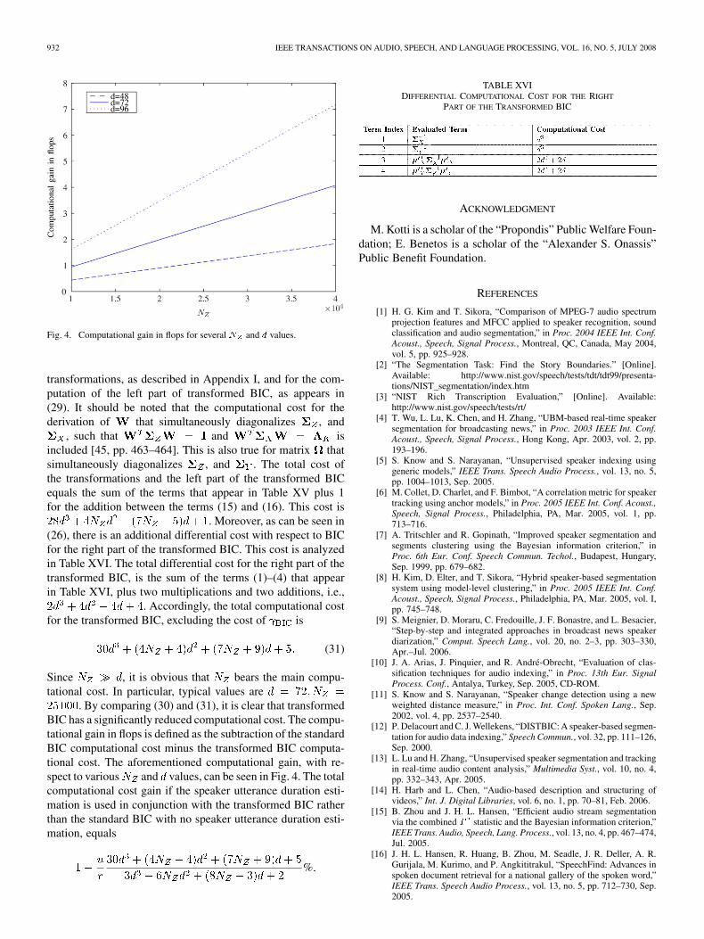
Fig. 4. Computational gain in flops for several N and d values.

transformations, as described in Appendix I, and for the com-putation of the left part of transformed BIC, as appears in(29). It should be noted that the computational cost for thederivation of that simultaneously diagonalizes , and

, such that and isincluded [45, pp. 463–464]. This is also true for matrix thatsimultaneously diagonalizes , and . The total cost ofthe transformations and the left part of the transformed BICequals the sum of the terms that appear in Table XV plus 1for the addition between the terms (15) and (16). This cost is

. Moreover, as can be seen in(26), there is an additional differential cost with respect to BICfor the right part of the transformed BIC. This cost is analyzedin Table XVI. The total differential cost for the right part of thetransformed BIC, is the sum of the terms (1)–(4) that appearin Table XVI, plus two multiplications and two additions, i.e.,

. Accordingly, the total computational costfor the transformed BIC, excluding the cost of is

(31)

Since , it is obvious that bears the main compu-tational cost. In particular, typical values are

. By comparing (30) and (31), it is clear that transformedBIC has a significantly reduced computational cost. The compu-tational gain in flops is defined as the subtraction of the standardBIC computational cost minus the transformed BIC computa-tional cost. The aforementioned computational gain, with re-spect to various and values, can be seen in Fig. 4. The totalcomputational cost gain if the speaker utterance duration esti-mation is used in conjunction with the transformed BIC ratherthan the standard BIC with no speaker utterance duration esti-mation, equals

%

TABLE XVIDIFFERENTIAL COMPUTATIONAL COST FOR THE RIGHT

PART OF THE TRANSFORMED BIC

ACKNOWLEDGMENT

M. Kotti is a scholar of the “Propondis” Public Welfare Foun-dation; E. Benetos is a scholar of the “Alexander S. Onassis”Public Benefit Foundation.

REFERENCES

[1] H. G. Kim and T. Sikora, “Comparison of MPEG-7 audio spectrumprojection features and MFCC applied to speaker recognition, soundclassification and audio segmentation,” in Proc. 2004 IEEE Int. Conf.Acoust., Speech, Signal Process., Montreal, QC, Canada, May 2004,vol. 5, pp. 925–928.

[2] “The Segmentation Task: Find the Story Boundaries.” [Online].Available: http://www.nist.gov/speech/tests/tdt/tdt99/presenta-tions/NIST_segmentation/index.htm

[3] “NIST Rich Transcription Evaluation,” [Online]. Available:http://www.nist.gov/speech/tests/rt/

[4] T. Wu, L. Lu, K. Chen, and H. Zhang, “UBM-based real-time speakersegmentation for broadcasting news,” in Proc. 2003 IEEE Int. Conf.Acoust., Speech, Signal Process., Hong Kong, Apr. 2003, vol. 2, pp.193–196.

[5] S. Know and S. Narayanan, “Unsupervised speaker indexing usinggeneric models,” IEEE Trans. Speech Audio Process., vol. 13, no. 5,pp. 1004–1013, Sep. 2005.

[6] M. Collet, D. Charlet, and F. Bimbot, “A correlation metric for speakertracking using anchor models,” in Proc. 2005 IEEE Int. Conf. Acoust.,Speech, Signal Process., Philadelphia, PA, Mar. 2005, vol. 1, pp.713–716.

[7] A. Tritschler and R. Gopinath, “Improved speaker segmentation andsegments clustering using the Bayesian information criterion,” inProc. 6th Eur. Conf. Speech Commun. Techol., Budapest, Hungary,Sep. 1999, pp. 679–682.

[8] H. Kim, D. Elter, and T. Sikora, “Hybrid speaker-based segmentationsystem using model-level clustering,” in Proc. 2005 IEEE Int. Conf.Acoust., Speech, Signal Process., Philadelphia, PA, Mar. 2005, vol. I,pp. 745–748.

[9] S. Meignier, D. Moraru, C. Fredouille, J. F. Bonastre, and L. Besacier,“Step-by-step and integrated approaches in broadcast news speakerdiarization,” Comput. Speech Lang., vol. 20, no. 2–3, pp. 303–330,Apr.–Jul. 2006.

[10] J. A. Arias, J. Pinquier, and R. André-Obrecht, “Evaluation of clas-sification techniques for audio indexing,” in Proc. 13th Eur. SignalProcess. Conf., Antalya, Turkey, Sep. 2005, CD-ROM.

[11] S. Know and S. Narayanan, “Speaker change detection using a newweighted distance measure,” in Proc. Int. Conf. Spoken Lang., Sep.2002, vol. 4, pp. 2537–2540.

[12] P. Delacourt and C. J. Wellekens, “DISTBIC: A speaker-based segmen-tation for audio data indexing,” Speech Commun., vol. 32, pp. 111–126,Sep. 2000.

[13] L. Lu and H. Zhang, “Unsupervised speaker segmentation and trackingin real-time audio content analysis,” Multimedia Syst., vol. 10, no. 4,pp. 332–343, Apr. 2005.

[14] H. Harb and L. Chen, “Audio-based description and structuring ofvideos,” Int. J. Digital Libraries, vol. 6, no. 1, pp. 70–81, Feb. 2006.

[15] B. Zhou and J. H. L. Hansen, “Efficient audio stream segmentationvia the combined T statistic and the Bayesian information criterion,”IEEE Trans. Audio, Speech, Lang. Process., vol. 13, no. 4, pp. 467–474,Jul. 2005.

[16] J. H. L. Hansen, R. Huang, B. Zhou, M. Seadle, J. R. Deller, A. R.Gurijala, M. Kurimo, and P. Angkititrakul, “SpeechFind: Advances inspoken document retrieval for a national gallery of the spoken word,”IEEE Trans. Speech Audio Process., vol. 13, no. 5, pp. 712–730, Sep.2005.


[17] M. Cettolo and M. Vescovi, “Efficient audio segmentation algorithmsbased on the BIC,” in Proc. 2003 IEEE Int. Conf. Acoust., Speech,Signal Process., Hong Kong, Apr. 2003, vol. 6, pp. 537–540.

[18] J. Ajmera, I. McCowan, and H. Bourlard, “Robust speaker change de-tection,” IEEE Signal Process. Lett., vol. 11, no. 8, pp. 649–651, Aug.2004.

[19] D. A. Reynolds and P. Torres-Carrasquillo, “Approaches and applica-tions of audio diarization,” in Proc. IEEE Int. Conf. Acoust., Speech,Signal Process., Philadelphia, PA, Mar. 2005, vol. 5, pp. 953–956.

[20] C. H. Wu, Y. H. Chiu, C. J. Shia, and C. Y. Lin, “Automatic segmenta-tion and identification of mixed-language speech using delta-BIC andLSA-based GMMs,” IEEE Trans. Audio, Speech, Lang. Process., vol.14, no. 1, pp. 266–276, Jan. 2006.

[21] M. Kotti, L. G. P. M. Martins, E. Benetos, J. S. Cardoso, and C.Kotropoulos, “Automatic speaker segmentation using multiple fea-tures and distance measures: A comparison of three approaches,” inProc. IEEE Int. Conf. Multimedia Expo, Toronto, ON, Canada, Jul.2006, pp. 1101–1104.

[22] C. H. Wu and C. H. Hsieh, “Multiple change-point audio segmentationand classification using an MDL-based Gaussian model,” IEEE Trans.Audio, Speech, Lang. Process., vol. 14, no. 2, pp. 647–657, Mar. 2006.

[23] S. Cheng and H. Wang, “Metric SEQDAC: A hybrid approach for audiosegmentation,” in Proc. 8th Int. Conf. Spoken Lang. Process., Jeju,Korea, Oct. 2004, pp. 1617–1620.

[24] F. Van der Heijden, R. P. W. Duin, D. de Ridder, and D. M. J. Tax,Classification, Parameter Estimation and State Estimation: An Engi-neering Approach Using MATLAB. London, U.K.: Wiley, 2004.

[25] N. A. Campbell, “Robust procedures in multivariate analysis I: Robustcovariance estimation,” Appl. Statist., vol. 29, no. 3, pp. 231–237, 1980.

[26] G. A. F. Seber, Multivariate Observations. New York: Wiley, 1994.[27] S. Tadjudin and D. A. Landgrebe, “Covariance estimation with limited

training samples,,” IEEE Trans. Geosci. Remote Sen., vol. 37, no. 4, pp.2113–2118, Jul. 1999.

[28] J. S. Garofolo, “DARPA TIMIT Acoustic-phonetic continuous speechcorpus,” in Linguistic Data Consortium, Philadelphia, PA, 1993.

[29] R. D. Reiss and M. Thomas, Statistical Analysis of Extreme Values.Basel, Germany: Birkhäuser Verlag, 1997.

[30] M. Kotti, E. Benetos, C. Kotropoulos, and I. Pitas, “A neural networkapproach to audio-assisted movie dialogue detection,” Neurocomput.,Special Iss.: Adv. Neural Netw. for Speech Audio Process., vol. 71, no.1–3, pp. 157–166, Dec. 2007.

[31] J. L. Folks and R. S. Chhikara, “The inverse Gaussian distribution andits statistical application—A review,” J. R. Statist. Soc. B, vol. 40, pp.263–289, 1978.

[32] N. L. Johnson, S. Kotz, and S. Balakrishnan, Continuous UnivariateDistributions. , New York: Wiley, 1994, vol. 1.

[33] S. I. Boyarchenko and S. Z. Levendorskii, “Perpetual American pro-cesses under Lèvi processes,” SIAM J. Control Optim., vol. 40, no. 6,pp. 1514–1516, Jun. 2001.

[34] M. C. K. Tweedie, “Statistical properties of inverse Gaussian distribu-tions I,” Ann. Math. Statist., vol. 28, no. 2, pp. 362–377, Jun. 1957.

[35] X. D. Huang, A. Acero, and H.-S. Hon, Spoken Language Processing:A Guide to Theory, Algorithm, and System Development. Upper RiverSaddle, NJ: Pearson Education–Prentice-Hall, 2001.

[36] R. Kohavi and G. H. John, “Wrappers for feature subset selection,”Artif. Intell., vol. 97, no. 1–2, pp. 273–324, Dec. 1997.

[37] G. Almpanidis and C. Kotropoulos, “Phonemic segmentation using thegeneralised Gamma distribution and small sample Bayesian informa-tion criterion,” Speech Commun., vol. 50, no. 1, pp. 38–55, Jan. 2008.

[38] M. Kotti, V. Moschou, and C. Kotropoulos, “Speaker segmentation andclustering,” Signal Process., vol. 88, no. 5, pp. 1091–1124, May 2008.

[39] J. J. Barnette and J. E. McLean, “The Tukey honestly significant dif-ference procedure and its control of the type I error-rate,” in Proc.Annu. Meeting Mid-South Edu. Res. Assoc., New Orleans, LA, 1998,CD-ROM.

[40] C. Barras, X. Zhu, S. Meignier, and J. L. Gauvain, “Multistage speakerdiarization of broadcast news,” IEEE Trans. Audio Speech, Lang.Process., vol. 14, no. 5, pp. 1505–1512, Sep. 2006.

[41] J. Fiscus, “1997 English broadcast news speech (HUB4),” LinguisticData Consortium, Philadelphia, PA, 1998.

[42] D. Graff, J. Fiscus, and J. Garofolo, “1997 HUB4 English evaluationspeech and transcripts,” Linguistic Data Consortium, Philadelphia, PA,2002.

[43] R. R. Korfhage, Information Storage and Retrieval. New York:Wiley, 1997.

[44] S. Strassel, C. Walker, and H. Lee, “RT-03 MDE training data speech,”Linguistic Data Consortium, Philadelphia, PA, 2004.

[45] G. H. Golub and C. F. Van Loan, Matrix Computations, 3rd ed. Bal-timore, MD: Johns Hopkins Univ. Press, 1996.

Margarita Kotti received the B.Sc. degree (withhonors) in informatics from the Department ofInformatics, Aristotle University of Thessaloniki,Thessaloniki, Greece, in 2005. She is currentlyworking towards the Ph.D. degree at the ArtificialIntelligence and Information Analysis Laboratory,Department of Informatics, Aristotle University ofThessaloniki.

She has worked as a Research Assistant in the Arti-ficial Intelligence and Information Analysis Labora-tory, Department of Informatics, Aristotle University

of Thessaloniki. Her research interests lie in the areas of speech and audio pro-cessing, pattern recognition, speaker segmentation, and emotion recognition.She has published three journal and 13 conference papers.

Ms. Kotti received scholarships and awards from the State Scholarship Foun-dation and she is currently a Scholar of the Propondis Public Welfare Founda-tion. She is a member of the Greek Computer Society.

Emmanouil Benetos received the B.Sc. degree (withhonors) in informatics and the M.Sc. degree (withhonors) in digital media, both from the AristotleUniversity of Thessaloniki, Thessaloniki, Greece, in2005 and 2007, respectively.

He worked as a Researcher in the Artificial Intel-ligence and Information Analysis Laboratory, Aris-totle University of Thessaloniki, from 2004 to 2007.His research interests include audio and speech pro-cessing, music information retrieval, computationalintelligence, and speech synthesis. He authored two

journal and 13 conference papers. He contributed one chapter to an edited bookin his areas of expertise.

Mr. Benetos received a scholarship for outstanding achievement in sciencesby the Greek Scholarship Institution and he was a Scholar of the AlexanderS. Onassis Public Benefit Foundation. He is a member of the Greek ComputerSociety.

Constantine Kotropoulos (SM’06) was born inKavala, Greece, in 1965. He received the Diplomadegree (with honors) in electrical engineeringand the Ph.D. degree in electrical and computerengineering, both from the Aristotle University ofThessaloniki, Thessaloniki, Greece, in 1988 and1993, respectively.

He is currently an Associate Professor in theDepartment of Informatics, Aristotle University ofThessaloniki. From 1989 to 1993, he was a Researchand Teaching Assistant in the Department of Elec-

trical and Computer Engineering at the same university. In 1995, he joinedthe Department of Informatics at the Aristotle University of Thessaloniki as aSenior Researcher and served then as a Lecturer from 1997 to 2001 and as anAssistant Professor from 2002 to 2007. He has also conducted research in theSignal Processing Laboratory at Tampere University of Technology, Tampere,Finland, during the summer of 1993. He has coauthored 33 journal papers, 142conference papers, and contributed five chapters to edited books in his areasof expertise. He is coeditor of the book Nonlinear Model-Based Image/VideoProcessing and Analysis (Wiley, 2001). His current research interests includeaudio, speech, and language processing, signal processing, pattern recognition,multimedia information retrieval, biometric authentication techniques, andhuman-centered multimodal computer interaction.

Prof. Kotropoulos was a scholar of the State Scholarship Foundation ofGreece and the Bodossaki Foundation. He is a senior member of the IEEE anda member of EURASIP, IAPR, ISCA, and the Technical Chamber of Greece.

Computationally Efficient and Robust BIC-Based Speaker Segmentation

Documents

Transcript of Computationally Efficient and Robust BIC-Based Speaker Segmentation