Comparative Analysis of Ledoit’s Covariance Matrixand Comparative Adjustment Liability Management

(CALM) Model

Within the Markowitz Framework

by

Yafei ZhangGregory McArthur

A Project Report

Submitted to the Faculty

of the

WORCESTER POLYTECHNIC INSTITUTE

In partial fulfillment of the requirements for the

Degree of Master of Science

in

Financial Mathematics

by

May 2014

APPROVED:

Professor Marcel Y. Blais, Capstone Advisor

Professor Luca Capogna, Head of Department

Abstract

Estimation of the covariance matrix of asset returns is a key com-ponent of portfolio optimization. Inherent in any estimation techniqueis the capacity to inaccurately reflect current market conditions. Typ-ical of Markowitz portfolio optimization theory, which we use as thebasis for our analysis, is to assume that asset returns are stationary.This assumption inevitably causes an optimized portfolio to fail duringa market crash since estimates of covariance matrices of asset returnsno longer reflect current conditions. We use the market crash of 2008to exemplify this fact. A current industry-standard benchmark forestimation is the Ledoit covariance matrix, which attempts to adjusta portfolio’s aggressiveness during varying market conditions. We testthis technique against the CALM (Covariance Adjustment for Liabil-ity Management Method), which incorporates forward-looking signalsfor market volatility to reduce portfolio variance, and assess undercertain criteria how well each model performs during recent marketcrash. We show that CALM should be preferred against the sampleconvariance matrix and Ledoit covariance matrix under some reason-able weight constraints.

Key Words: covariance matrix estimation, Ledoit’s model, shrink-age parameter, CALM, forward looking signal

ii

ACKNOWLEDGMENTS

We would like to thank, first and foremost, Marcel Blais, PhD, for hiscontinued interest in the topic of covariance matrix estimation. Becauseof him we were able to continue this study as part of our requirement for aMasters of Financial Mathematics at Worcester Polytechnic Institute (WPI).Since this project is a continuation of a Summer 2012 REU study at WPI,we would also like to thank all those who partook in formulation of the topicof Incorporating Forward-Looking Signals Into Covariance Estimation ForPortfolio Optimization. Namely, this includes: Marcel Blais, Carlos Morales,Tejpal S. Ahluwalia, Robert P. Hark, Daniel R. Helkey, and Nicholas F.Marshall. Finally, we would like to the thank the Mathematical SciencesDepartment at WPI for their resources and guidance.

iii

Contents

1 Introduction 1

2 Background 32.1 Ledoit’s Model . . . . . . . . . . . . . . . . . . . . . . . . . . 3

2.1.1 Statistical Model . . . . . . . . . . . . . . . . . . . . . 32.1.2 Sample Covariance Matrix . . . . . . . . . . . . . . . . 32.1.3 Single-Index Covariance Matrix Estimator . . . . . . . 42.1.4 Formula for the Optimal Shrinkage Intensity . . . . . . 5

2.2 CALM Model . . . . . . . . . . . . . . . . . . . . . . . . . . . 82.2.1 The Choice of Constant ρhigh . . . . . . . . . . . . . . 8

3 Empirical Results 113.1 Assets Overview . . . . . . . . . . . . . . . . . . . . . . . . . . 113.2 Test for Properties of a Covariance Matrix . . . . . . . . . . . 123.3 Tangency Weight Programming . . . . . . . . . . . . . . . . . 143.4 Comparison Across Models . . . . . . . . . . . . . . . . . . . . 15

3.4.1 Holding period return . . . . . . . . . . . . . . . . . . 153.4.2 Leverage Ratio . . . . . . . . . . . . . . . . . . . . . . 163.4.3 Yearly Return Comparison Across Models . . . . . . . 163.4.4 Performance Ratio . . . . . . . . . . . . . . . . . . . . 193.4.5 Normal Distribution Fitting . . . . . . . . . . . . . . . 223.4.6 Tests for Normality . . . . . . . . . . . . . . . . . . . . 23

4 Conclusion 29

A Appendix 30A.1 Matlab Code . . . . . . . . . . . . . . . . . . . . . . . . . . . 30

iv

List of Figures

1 Yearly Performance Comparison Across Models . . . . . . . . 172 Yearly Normal Distribution Fitting Result for Markowitz model

with constraint [-0.2, 0.2] . . . . . . . . . . . . . . . . . . . . . 243 Yearly Normal Distribution Fitting Result for Ledoit’s model

with constraint [-0.2, 0.2] . . . . . . . . . . . . . . . . . . . . . 254 Yearly Normal Distribution Fitting Result for CALM 0.7 model

with constraint [-0.2, 0.2] . . . . . . . . . . . . . . . . . . . . . 265 Yearly Normal Distribution Fitting Result for CALM 0.9 model

with constraint [-0.2, 0.2] . . . . . . . . . . . . . . . . . . . . . 276 Q-Q Plot for Four [-0.2, 0.2] Constrained Models . . . . . . . . 28

v

1

1 Introduction

This work is a continuation of the Summer 2012 WPI Center for IndustrialMathematics & Statistics NSF funded Research Experience for Undergrad-uates (REU) Financial Mathematics project sponsored by Wellington Man-agement. The project remained under the direction of WPI Professor MarcelBlais and includes work from Masters candidates Yafei Zhang and GregoryMcArthur.

A well-known problem with Markowitz portfolio theory is the assumptionof stationarity of asset returns [12]. In other words, the joint distribution ofasset returns does not change over time. The covariance matrix of asset re-turns is used to determine, in a Markowitz setting, how much an investorshould choose to hold in the context of diversification. This calculation isused to create a mean-variance portfolio, which determines how much riskwe will have to incur for an expected return. Accurately estimating a co-variance matrix is important to the study of portfolio optimization and riskmanagement.

Markowitz originally proposed using the sample covariance matrix; how-ever, we have come to realize that this is certainly not the best technique.Essentially when the number of stocks, N , is large relative to the historicaldata, estimation error occurs. Also since Markowitz portfolio theory assumesthe stationarity of asset returns, a sample covariance matrix tells us nothingabout how to invest given a variety of possible market changes.

Designing a covariance matrix estimate that can work around this issuehas been an important study for many years. Currently, the Ledoit [1] covari-ance matrix is one of the industry-standard benchmarks. In order to reflectmarket reality, Ledoit developed a shrinkage parameter, which can adjustthe aggressiveness of a portfolio automatically according to different marketconditions. We show in this paper that Ledoit is certainly a good choice, butthat under certain mathematical conditions, other models may be preferred.In our case, we test against the CALM (Covariance Adjustment for LiabilityManagement) model.

CALM originated from the Summer 2012 REU Financial Mathematicsproject at WPI. The aim of CALM is to use shrinkage based informationon forward-looking signals to create a covariance matrix that better reflectsmarket conditions. Essentially the goal is to try and improve upon the Ledoitcovariance matrix. For more information on this topic, we refer to Incorporat-

2

ing Forward-Looking Signals Into Covariance Matrix Estimation for PortfolioOptimization [2] .

We study the mathematics behind the two models and compare theirperformance in last financial crisis from 2007 to 2009.

3

2 Background

This section attempts to explain the mathematics behind the shrinkage esti-mator of the covariance matrix introduced by Ledoit.

2.1 Ledoit’s Model

2.1.1 Statistical Model

We first focus on understanding the Ledoit technique [1] for estimating thecovariance matrix of stock returns, as it is currently an industry-standard.

Let X denote an N×T matrix of T observations on a system of N randomvariables representing T returns on a universe of N stocks.

Assumption 1. Stock returns are independent and indentically dstributed(iid) through time and are not assumed to be normally distributed.

This assumption implies that the time-series representing stock returnsare stationary. We note that actual stock returns do not verify this assump-tion.

Assumption 2. The number of stocks N is fixed and finite, while the numberof observations T goes to infinity.

Assumption 3. Stock returns have a finite fourth moment:

∀ i, j, k, l = 1, . . . , n ∀ t = 1, . . . , T E [|xitxjtxktxlt|] <∞.

A fourth moment is a measure of the peak of a distribution. A finitefourth moment implies that a peak is not infinite, and hence we have a finitevariance (and covariance) and can apply the central limit theorem.

2.1.2 Sample Covariance Matrix

We define the sample mean vector m and the sample covariance matrix Sby:

m =1

TX1,

4

and

S =1

TX

(I− 1

T11′)X′. (1)

Here, 1 is a conformable vector of 1’s, 1′ represents its transpose. S representsa T × 1 vector of ones, I is a T × T identity matrix.

2.1.3 Single-Index Covariance Matrix Estimator

Sharpe’s single-index model assumes that stock returns are generated by:

xit = αi + βix0t + εit. (2)

Here the residuals V arεit are uncorrelated to market returns x0t and to oneanother. We also have that V ar (εit) = δii, which gives that the variancebetween stocks is constant. We can see this by taking V ar (xit) ,∀t.

The covariance matrix implied by this model is:

Φ = σ200ββ

′ + ∆. (3)

Here σ200 is the N × N covariance matrix of market returns, β is the N × 1

vector of slopes, and ∆ is the N × N diagonal matrix containing residualvariances δii. We denote φij by the (i, j)-th entry of Φ.

We note that this model can be estimated by running a regression of stocki′s returns on the market. Call bi the slope estimate and dii the residualvariance estimate, then the single-index model yields the following estimatorfor the covariance matrix of stock returns:

F = s200bb′ + D. (4)

Here, s200 is the sample variance of market returns, b is the vector of slope es-timates, and D is the diagonal matrix containing residual variance estimatesdii. Call fij the (i, j)-th entry of F.

Assumption 4. Φ 6= Σ, where Σ is the sample covariance matrix.

Assumption 5. The returns of market portfolio has positive variance, thatis, σ2

00 > 0.

5

2.1.4 Formula for the Optimal Shrinkage Intensity

In order to understand the Ledoit covariance matrix, we need to understandshrinkage.

When considering a large number of stocks, the estimated sample co-variance matrix tends to have a large error. The error implies that extremecoefficients tend to not be representative of the true covariance matrix. This,in turn, causes a mean-variance portfolio optimizer to place its biggest betson those coefficients which are extremely unreliable.

The main idea behind shrinkage is that coefficients with positive errorneed to be compensated for by pulling them downward and the reverse forcoefficients with negative error. Essentially we are shrinking the error to-wards the center.

We need to question what it is we are shrinking and to what intensity.Consider the model:

Fδ + (1− δ)S. (5)

F is defined by (4), S by (1), and δ is our shrinkage estimate to be found.We consider a quadratic loss function defined by:

L (δ) = ‖δF + (1− δ)S − Σ‖2F . (6)

Notice how we are calculating the distance between our shrinkage modeland the sample covarance matrix of stock returns, Σ. This is a quadraticmeasure of distance between the true and the estimated covariance matricesbased on the Frobenius norm.

Now consider

R (δ) = E [L (δ)] . (7)

We can rewrite (7) in summation form which considers the components ofthe matrices. This in conjunction with (6) yields

6

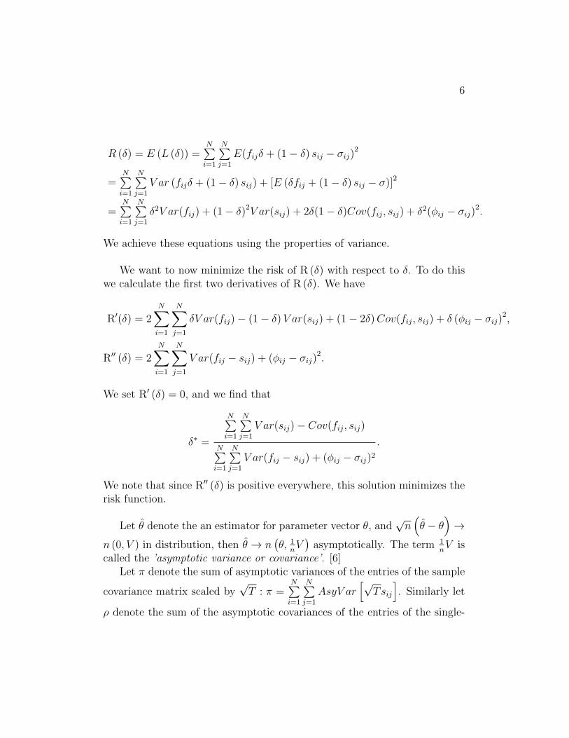
R (δ) = E (L (δ)) =N∑i=1

N∑j=1

E(fijδ + (1− δ) sij − σij)2

=N∑i=1

N∑j=1

V ar (fijδ + (1− δ) sij) + [E (δfij + (1− δ) sij − σ)]2

=N∑i=1

N∑j=1

δ2V ar(fij) + (1− δ)2V ar(sij) + 2δ(1− δ)Cov(fij, sij) + δ2(φij − σij)2.

We achieve these equations using the properties of variance.

We want to now minimize the risk of R (δ) with respect to δ. To do thiswe calculate the first two derivatives of R (δ). We have

R′(δ) = 2N∑i=1

N∑j=1

δV ar(fij)− (1− δ)V ar(sij) + (1− 2δ)Cov(fij, sij) + δ (φij − σij)2,

R′′ (δ) = 2N∑i=1

N∑j=1

V ar(fij − sij) + (φij − σij)2.

We set R′ (δ) = 0, and we find that

δ∗ =

N∑i=1

N∑j=1

V ar(sij)− Cov(fij, sij)

N∑i=1

N∑j=1

V ar(fij − sij) + (φij − σij)2.

We note that since R′′ (δ) is positive everywhere, this solution minimizes therisk function.

Let θ̂ denote the an estimator for parameter vector θ, and√n(θ̂ − θ

)→

n (0, V ) in distribution, then θ̂ → n(θ, 1

nV)

asymptotically. The term 1nV is

called the ’asymptotic variance or covariance’. [6]Let π denote the sum of asymptotic variances of the entries of the sample

covariance matrix scaled by√T : π =

N∑i=1

N∑j=1

AsyV ar[√

Tsij

]. Similarly let

ρ denote the sum of the asymptotic covariances of the entries of the single-

7

index covariance matrix with the entries of the sample covariance matrix

scaled by√T : ρ =

N∑i=1

N∑j=1

AsyCov[√

Tfij,√Tsij

]. Finally let γ measure the

misspecification of the single-index model: γ =N∑i=1

N∑j=1

(φij − σij)2. Then the

optimal shrinkage δ∗ satisfies: [1]

δ∗ =1

T

π − ργ

+O(

1

T 2

). (8)

From equation (8), we have that:

Tδ∗ =

N∑i=1

N∑j=1

V ar(√Tsij)− Cov(

√Tfij,

√Tsij)

N∑i=1

N∑j=1

V ar(fij − sij) + (φij − σij)2.

Using the assumptions 1 and 3, that the data is iid and from finite fourthmoments, we have that:

N∑i=1

N∑j=1

V ar(√Tsij)→ π,

N∑i=1

N∑j=1

Cov(√Tfij,

√Tsij)→ ρ,

N∑i=1

N∑j=1

V ar(fij − sij) = O(1

T).

Hence the optimal shrinkage is constant k = π−ργ

[1] .Finally, using this notation, the shrinkage estimator for the stock return

covariance matrix that Ledoit recommend is:

S =k

TF + (1− k

T)S. (9)

8

Since the shrinkage estimator captures the current market status, it con-tains forward looking signal that will make the covariance matrix estimatemore responsive to the changes in market.

2.2 CALM Model

Covariance Adjustment for Liability Management (CALM) is a new modelthat incorporates signals for market volatility to minimize portfolio variance.This model originated from the REU aforementioned in the Introductionsection of this paper.[2].

We wish to construct a covariance matrix such that it accurately reflectsa stressed market. Stressed market regimes are commonly observed to havehigher correlations between stocks [3]. We shall try to account for this prop-erty by incorporating high correlations into a stressed covariance matrix, H.We construct a covariance matrix with constant high correlation with themethod used by Bollerslev [4].

Let C be a high correlation matrix with a constant high correlation. ThenCi,i = 1 and Ci,j = ρhigh. Let V be the diagonal volatility matrix. Then,

H = VCV (10)

We call H the stressed covariance matrix and expect that when the mar-ket is in turmoil, ρhigh approximates the stock correlations and H approxi-mates Σ. In addition we continue to use the shrinkage parameter defined inLedoit’s Model to balance the weights between the sample covariance matrixS and highly structured matrix H.

2.2.1 The Choice of Constant ρhigh

A qualified highly structured correlation matrix should also be invertible. Wederive the range of ρhigh in which the correlation matrix is positive definiteand thus invertible.

Let p denote the constant value of ρhigh and C denote the N ×N highly

9

structured correlation matrix,

C =

1 p p · · · pp 1 p · · · pp p 1 · · · p...

......

. . ....

p p p · · · 1

.

We calculate the 1st to 3rd principle minor of C below:

∆1 = 1,∆2 = 1− p2,∆3 = 2p3 − 3p2 + 1 = (1− p)2 (1 + 2p) .

Further C′s 4th principle minor is:

∆4 = (1− p)3 (1 + 3p) . (11)

The N th principle minor is

∆n = (1− p)n−1 [1 + (n− 1) p] .

We calculate the determinant of C using Gaussian elimination∣∣∣∣∣∣∣∣∣∣∣

1 p p · · · pp 1 p · · · pp p 1 · · · p...

......

. . ....

p p p · · · 1

∣∣∣∣∣∣∣∣∣∣∣=

∣∣∣∣∣∣∣∣∣∣∣

1 + (n− 1)p 1 + (n− 1)p 1 + (n− 1)p · · · 1 + (n− 1)pp 1 p · · · pp p 1 · · · p...

......

. . ....

p p p · · · 1

∣∣∣∣∣∣∣∣∣∣∣

= [1 + (n− 1) p]

∣∣∣∣∣∣∣∣∣∣∣

1 1 1 · · · 1p 1 p · · · pp p 1 · · · p...

......

. . ....

p p p · · · 1

∣∣∣∣∣∣∣∣∣∣∣= [1 + (n− 1) p]

∣∣∣∣∣∣∣∣∣∣∣

1 1 1 · · · 10 1− p 0 · · · 00 0 1− p · · · 0...

......

. . ....

0 0 0 · · · 1− p

∣∣∣∣∣∣∣∣∣∣∣= [1 + (n− 1) p] (1− p)n−1 = ∆n.

In order to be positive definite, each kth principle minor of C has to be

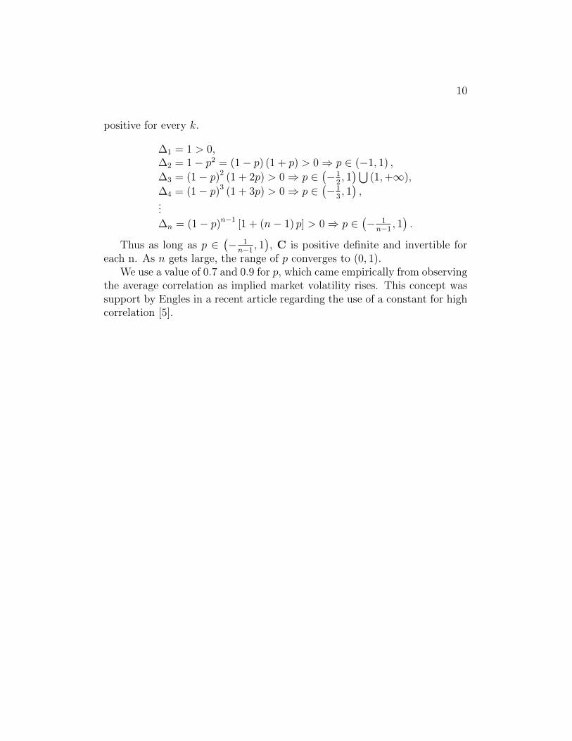
10

positive for every k.

∆1 = 1 > 0,∆2 = 1− p2 = (1− p) (1 + p) > 0⇒ p ∈ (−1, 1) ,

∆3 = (1− p)2 (1 + 2p) > 0⇒ p ∈(−1

2, 1)⋃

(1,+∞),

∆4 = (1− p)3 (1 + 3p) > 0⇒ p ∈(−1

3, 1),

...

∆n = (1− p)n−1 [1 + (n− 1) p] > 0⇒ p ∈(− 1n−1 , 1

).

Thus as long as p ∈(− 1n−1 , 1

), C is positive definite and invertible for

each n. As n gets large, the range of p converges to (0, 1).We use a value of 0.7 and 0.9 for p, which came empirically from observing

the average correlation as implied market volatility rises. This concept wassupport by Engles in a recent article regarding the use of a constant for highcorrelation [5].

11

3 Empirical Results

In order to test the portfolio performance under different covariance matrixestimates, we use Markowitz optimization theory [7] to calculate tangencyweights on a standard Markowitz model, and also Ledoit’s model and theCALM model [2] with constant correlation 0.7 and 0.9.

Markowitz portfolio theory is based on the assumption that the pastmarket behavior is consistent with future behavior. We relax this assumptionhere, assuming that market behavior changes dramatically during a crisis.We examine how the covariance matrix estimates change after implementingthe forward-looking signals from a crisis across the four different models. Wechoose weekly data from 2007 to 2009 as our holding period to perform theback-testing. This time interval allows us to test under a pre-crisis bubble,the actual crash, and the steady market recovery.

The key method we used to obtain the historical data is from a slidingwindow observation. A sliding window observation considers data from thepast n days and is applied each day starting from the n+ 1 day. Our holdingperiod is designed to be 3 years. We use 1 year as our length of slidingwindow. In order to simplify our project, we used a rectangular window, inwhich every past net return has a weight of 1.

A popular approach to manage risk is through diversification. Considerour portfolio as a linear combination of N risky assets; investing in a diversi-fied portfolio can help to reduce the risk from market changes and lower theportfolio volatility as long as the assets correlation coefficient is less than 1.

3.1 Assets Overview

Our portfolio is composed by 29 stocks traded on the NYSE. The constructionof our portfolio is based on following principles:

1. Diversification: Markowitz portfolio theory is especially useful whenthe portfolio contains a significant number of assets. Since market in-dices are generally well diversified, investing in a market index is areasonable choice. The Dow Jones Industrial Average only contains 30stocks and we decided to construct our portfolio by investing in everycomponent of the the Dow. Since our back-test starts at the beginningof 2007, we use the historical components of the Dow as of Nov 21,2005.

12

One of the major historical components of the Dow in 2005 was Gen-eral Motor Corporation (GM). GM Corporation filed for bankruptcyon July 8 2009, making its historical prices unattainable for the lateholding period. So we exclude GM Corporation, and for that reasonthere are only 29 stocks in our portfolio, rather than 30.

2. Fully invested: All of our available capital is invested in the riskyassets.

3.2 Test for Properties of a Covariance Matrix

Before using these estimators of a covariance matrix to calculate our tan-gency weights, we first need to make sure that these estimators contain someessential necessary properties of a covariance matrix.

A covariance matrix should have the following property:

• The covariance matrix must be a positive semi-definite matrix.

Standard Markowitz Model: Our covariance matrix estimator is thesample covariance matrix, S.

First, Let X denote an N × T matrix of T observations on a vector ofN random variables representing T returns on a universe of N stocks. Let1 denote a conformable vector of ones and I denote a conformable identitymatrix. We assume that N is a finite number while T goes to infinity. Wenote that

(I− 1

T11′)

is a T × T matrix, X′ is a T ×N matrix.

S =1

TX

(I− 1

T11′)X′. (12)

Given two matrices, A and B, we know that the rank of the product ABis less than or equal to the minimum of the ranks of A and B i.e.,

rank (AB) ≤ min {rank (A) , rank (B)} . (13)

Applying (12) to property (13), we get:

rank (S) = rank

(1

TX

(I− 1

T11′)X′)≤ min

{rank (X) , rank

(I− 1

T11′)}

,

13

where X is assumed to have full rank since we can take X inverse. Thus(I− 1

T11′)

has smaller rank than X. As a result

rank (S) ≤ rank

(I− 1

T11′).

Using Gaussian elimination, we can show that

rank

(I− 1

T11′)

= T− 1.

Thusrank (S) ≤ T− 1.

As an N ×N matrix, as long as T > N , S has full rank and is invertible.In our portfolio, N = 29 and T = 3 × 52 = 156. Notice that T is larger

than N . Hence, S is invertible.Since the sample covariance matrix S is also a covariance matrix, it is posi-

tive semi-definite. Thus the estimator S does not lose this necessart property.

Ledoit Model: Our covariance matrix estimator is kTF + (1− k

TS).

As stated before, F is the covariance matrix implied by the single factormodel. Since F is also a covariance matrix, it is positive semi-definite as well.

We know that if M is positive semi-definite and r > 0 is a real number,then rM is positive semi-definite. If M and N are positive semi-definite,then M + N is also positive semi-definite. Since our shrinkage parameter k

T

is between 0 and 1, kTH+ (1− k

TS) is also positive semi-definite. Ledoit’s es-

timator, implemented in the Markowitz portfolio framework, maintains thisnecessary property of a covariance matrix.

CALM Model: Our covariance matrix estimator is kTH + (1 − k

TS),

where H is as defined in (10).Here S is the same sample covariance matrix used within the standard

Markowitz model, so it is positive semi-definite. As we previously proved, aslong as the off-diagonal constant number p ∈ (0, 1), all kth principle minorsof H are positive and hence H is also positive definite, which implies H mustbe positive semi-definite. For the same reason, since shrinkage parameter k

T

is between 0 and 1, kTH + (1− k

TS) is positive semi-definite.

We can conclude that the CALM estimator also has the desired propertyof a covariance matrix.

14

3.3 Tangency Weight Programming

As stated before, the length of our sliding window is 1 year. US Treasurybills are issued by the United States government, which can be consideredfree of risk. To match the window length, we choose the return of the 1 yearTreasury bill as our risk-free rate. The data was obtained from the FederalReserve’s website [11].

The unconstrained tangency portfolio is useful theoretically, but has sev-eral problems in practice. The method requires the inverse of the covariancematrix; however, numerical error can occur when the covariance matrix isnearly singular. In addition, elements of w (the portfolio weights) can benegative, which represents shorting assets. This involves borrowing stockon margin, which is a form of leveraging and easily can trigger margin calls.Moreover, the unconstrained method for obtaining a minimum variance port-folio does not limit portfolio turnover. The weight vector can change sub-stantially without restriction between time periods, which means that assetturnover has the potential to be high, and we may need to long or shortlarge amounts of stock on each rebalance date. In practice this causes trans-action fees to cut into profit. In order to avoid large negative weights andmargin calls, we used constrained quadratic programming. Quadratic pro-gramming is used to minimize a quadratic objective function subject to linearconstraints [12]. In this project we try the following two constraints.

1. We permit shorting stocks but limit the maximum shorting weight tobe -0.2 and the maximum longing weight to be 0.2.

2. We prohibit short selling, limiting all tangency weights to be between0 and 1.

We calculate unconstrained weights and two different constrained weightsfor the four models and compared their return distributions. Hence we have12 models to analyze. We used MATLAB to calculate the initial tangencyportfolio weights and formed our portfolio beginning on Jan 1, 2007. Ourprinciple amount was $1 million. During the holding period we used weeklyreturns and rebalanced the portfolio monthly.

15

3.4 Comparison Across Models

3.4.1 Holding period return

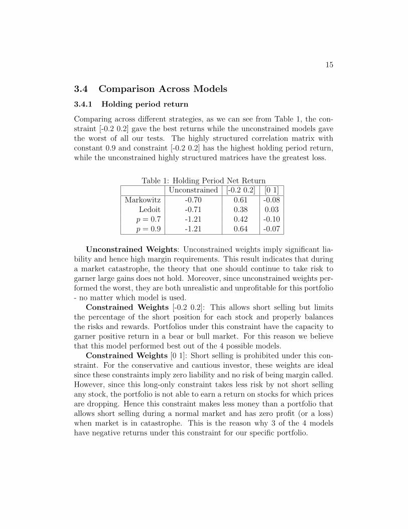
Comparing across different strategies, as we can see from Table 1, the con-straint [-0.2 0.2] gave the best returns while the unconstrained models gavethe worst of all our tests. The highly structured correlation matrix withconstant 0.9 and constraint [-0.2 0.2] has the highest holding period return,while the unconstrained highly structured matrices have the greatest loss.

Table 1: Holding Period Net ReturnUnconstrained [-0.2 0.2] [0 1]

Markowitz -0.70 0.61 -0.08Ledoit -0.71 0.38 0.03p = 0.7 -1.21 0.42 -0.10p = 0.9 -1.21 0.64 -0.07

Unconstrained Weights: Unconstrained weights imply significant lia-bility and hence high margin requirements. This result indicates that duringa market catastrophe, the theory that one should continue to take risk togarner large gains does not hold. Moreover, since unconstrained weights per-formed the worst, they are both unrealistic and unprofitable for this portfolio- no matter which model is used.

Constrained Weights [-0.2 0.2]: This allows short selling but limitsthe percentage of the short position for each stock and properly balancesthe risks and rewards. Portfolios under this constraint have the capacity togarner positive return in a bear or bull market. For this reason we believethat this model performed best out of the 4 possible models.

Constrained Weights [0 1]: Short selling is prohibited under this con-straint. For the conservative and cautious investor, these weights are idealsince these constraints imply zero liability and no risk of being margin called.However, since this long-only constraint takes less risk by not short sellingany stock, the portfolio is not able to earn a return on stocks for which pricesare dropping. Hence this constraint makes less money than a portfolio thatallows short selling during a normal market and has zero profit (or a loss)when market is in catastrophe. This is the reason why 3 of the 4 modelshave negative returns under this constraint for our specific portfolio.

16

3.4.2 Leverage Ratio

Table 2: Leverage RatioUnconstrained [-0.2 0.2] [0 1]

Markowitz 27.4 3.4 1.0Ledoit 5.8 2.6 1.0p = 0.7 22.5 3.1 1.0p = 0.9 22.5 3.4 1.0

Leverage =

n∑i=1

|wi|n∑i=1

wi

(14)

The Leverage ratio is defined as the sum of absolute value of each tangencyweight divided by the sum of each tangency weight. Unconstrained portfoliooptimization models may introduce significant short sell positions. Therefore,as we can see from the Table 2, their leverage ratios are also very high. How-ever, portfolios with a large leverage ratio are not only very risky (as statedbefore, they have unlimited potential liability) but also have to meet largemargin requirements. Rarely is a portfolio manager is willing to constructhis or her portfolio using unconstrained weights. Since unconstrained modelsare neither realistic nor profitable, we consider the unconstrained cases onlyas basic case general models but not as practical models. The rest of thisreport only analyzes the performances of 8 constrained models.

3.4.3 Yearly Return Comparison Across Models

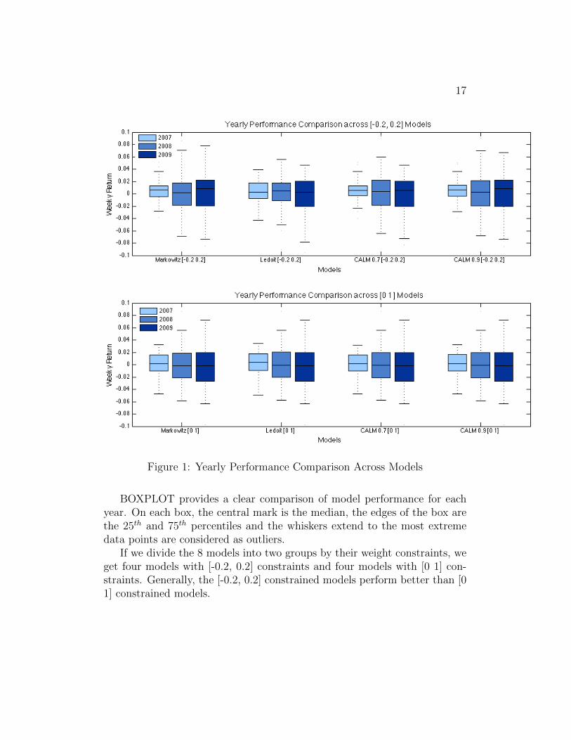
As stated before, we use weekly data to calculate the expected returns andcovariance matrix estimates and rebalance the portfolio on the first day ofeach month according to the new tangency weights. During each month wehold the portfolio and do not make any changes. We only observe and trackthe portfolios’ weekly performances based on the monthly initial weights. Atthe end of holding period we collect 156 returns for each model. We plot theweekly returns in MATLAB using a BOXPLOT function and group by yearand model. We can see this in Fig. 1.

17

Figure 1: Yearly Performance Comparison Across Models

BOXPLOT provides a clear comparison of model performance for eachyear. On each box, the central mark is the median, the edges of the box arethe 25th and 75th percentiles and the whiskers extend to the most extremedata points are considered as outliers.

If we divide the 8 models into two groups by their weight constraints, weget four models with [-0.2, 0.2] constraints and four models with [0 1] con-straints. Generally, the [-0.2, 0.2] constrained models perform better than [01] constrained models.

18

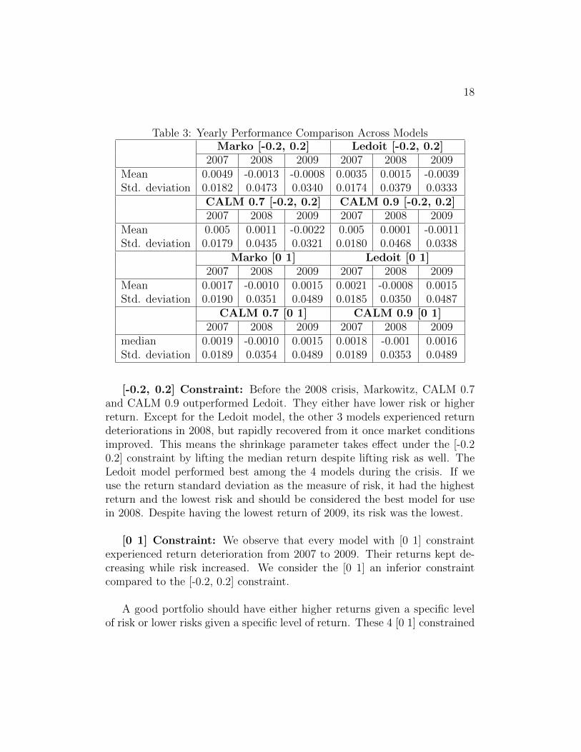
Table 3: Yearly Performance Comparison Across ModelsMarko [-0.2, 0.2] Ledoit [-0.2, 0.2]

2007 2008 2009 2007 2008 2009Mean 0.0049 -0.0013 -0.0008 0.0035 0.0015 -0.0039Std. deviation 0.0182 0.0473 0.0340 0.0174 0.0379 0.0333

CALM 0.7 [-0.2, 0.2] CALM 0.9 [-0.2, 0.2]2007 2008 2009 2007 2008 2009

Mean 0.005 0.0011 -0.0022 0.005 0.0001 -0.0011Std. deviation 0.0179 0.0435 0.0321 0.0180 0.0468 0.0338

Marko [0 1] Ledoit [0 1]2007 2008 2009 2007 2008 2009

Mean 0.0017 -0.0010 0.0015 0.0021 -0.0008 0.0015Std. deviation 0.0190 0.0351 0.0489 0.0185 0.0350 0.0487

CALM 0.7 [0 1] CALM 0.9 [0 1]2007 2008 2009 2007 2008 2009

median 0.0019 -0.0010 0.0015 0.0018 -0.001 0.0016Std. deviation 0.0189 0.0354 0.0489 0.0189 0.0353 0.0489

[-0.2, 0.2] Constraint: Before the 2008 crisis, Markowitz, CALM 0.7and CALM 0.9 outperformed Ledoit. They either have lower risk or higherreturn. Except for the Ledoit model, the other 3 models experienced returndeteriorations in 2008, but rapidly recovered from it once market conditionsimproved. This means the shrinkage parameter takes effect under the [-0.20.2] constraint by lifting the median return despite lifting risk as well. TheLedoit model performed best among the 4 models during the crisis. If weuse the return standard deviation as the measure of risk, it had the highestreturn and the lowest risk and should be considered the best model for usein 2008. Despite having the lowest return of 2009, its risk was the lowest.

[0 1] Constraint: We observe that every model with [0 1] constraintexperienced return deterioration from 2007 to 2009. Their returns kept de-creasing while risk increased. We consider the [0 1] an inferior constraintcompared to the [-0.2, 0.2] constraint.

A good portfolio should have either higher returns given a specific levelof risk or lower risks given a specific level of return. These 4 [0 1] constrained

19

models do not meet this criteria well. Since the U.S. equity market started torecover in 2009, the [0 1] constraints weakened the model’s ability to capturethis market characteristic and adjust shrinkage parameters in time.

Each model under [-0.2, 0.2] constraint has its own strengths; we willfocus on these 4 models in the following analysis.

3.4.4 Performance Ratio

It is not comprehensive to focus only on the final holding period returns. Inorder to compare the weekly performance over these 4 models, we calculatetheir Sharpe Ratio, Treynor Ratio and Information Ratio using the DJIA asa benchmark.

Sharpe’s RatioSharpe’s ratio (SR) is the industry standard for measuring risk-adjusted

return. Sharpe’s ratio is what reward an investor could expect on averagefor investing in a risky asset versus a risk-free asset. The numerator ofthe ratio is the expected portfolio return Rp less the risk-free rate Rf , andthe denominator is the portfolio return’s volatility or standard deviation ofreturns σp (less that of the risk-free asset’s standard deviation, which is zero).The resulting ratio isolates the expected excess return that the portfolio couldbe expected to generate per unit of portfolio return variability. Sharpe ratiouses actual instead of expected returns and is calculated as: [12]

Sharpe′sRatio =RP −Rf

σp.

Table 4: Sharpe’s Ratio from 2007 to 2009Unconstrained [-0.2 0.2] [0 1]

Markowitz -0.1714 0.2818 0.0142Ledoit -0.0291 0.2173 0.0419p = 0.7 -0.0635 0.2964 0.0169p = 0.9 -0.0635 0.2933 0.0170

Sharpe’s ratio informs an investor what portion of a portfolio’s perfor-mance is associated with risk taking. It measures a portfolio’s added valuerelative to its total risk. Table 4 shows the Sharpe’s Ratio for the 12 com-

20

binations of correlations and constraints. The risk-free rate is chosen to bethe 4-week treasury bill rate.

Generally Sharpe’s ratio is useful in pratice but it has its own set of limi-tations to consider. It is based on Markowitz portfolio theory, which proposesthat a portfolio can be described by just two measures: its mean return andits variance of returns. Sharpe’s ratio measures only one dimension of risk,the variance. Sharpe’s ratio is designed to be applied to investment strate-gies that have normal expected return distributions; it is not suitable formeasuring investments that are expected to have asymmetric returns. Thestudy on whether our portfolio has an asymmetric return will be performedby fitting a normal and a student t-distribution according to the parameterswe estimated from the available data. Details will be discussed later.

There are two obvious downfalls in using Sharpe’s Ratio [13], even in theframework of normally distributed returns:

• Sharpe’s ratio cannot tell an investor whether a high standard deviationis due to large upside deviations or downside deviations; the Sharperatio penalizes both equally.

• Negative Sharpe ratios, such as those arising during portfolio underperformance (which often occurs during bear markets) are also unin-formative.

For the CALM model with constant 0.9 and constraint [-0.2, 0.2], itsSharpe ratio is slightly smaller than the one with constant 0.7. However, ifwe look at their normal distribution fitting results, the mean for CALM 0.9is higher than CALM 0.7, along with their standard deviations, respectively.The normal fitting did not tell us whether this high standard deviation wasdue to large upside or downside deviations. Sharpe’s ratio does not distin-guish between them.

Treynor’s RatioLet σMP denote the return covariance between market portfolio and our

portfolio, and σ2M denote the market portfolio’s return variance, Treynor’s

ratio is defined as the following: [12]

Treynor′sRatio =RP −Rf

βp,

21

whereβp =

σMP

σ2M

.

Unlike Sharpe’s ratio, Treynor’s ratio (TR) uses beta in the denominatorinstead of the standard deviation. The beta measures only the portfolio’ssensitivity to the market movement, while the standard deviation is a mea-sure of the total volatility (upside as well as downside). The Treynor ratiorelates excess return over the risk-free rate to the additional risk taken; how-ever, systematic risk is used instead of total risk.[12] The Treynor ratio isinterpreted as excess returns per unit of systematic risk. As our portfoliocontains 29 stocks and can be considered well diversified, we can say that theeffect of unsystematic risk is very small. Table 5 summarizes the Treynor’sRatio of the 12 models.

Table 5: Treynor’s Ratio from 2007 to 2009Unconstrained [-0.2 0.2] [0 1]

Markowitz 0.1102 -0.0909 0.0114Ledoit 0.0088 -0.0445 0.0342p = 0.7 0.0108 -0.0753 0.0142p = 0.9 0.0108 -0.0842 0.0137

Among our 12 combinations of models and constraints, only long-onlyportfolios have a positive beta. This means only long-only portfolios are pos-itively correlated to market. Many negative TR appeared, which are uninfor-mative. The unconstrained Markowitz model had the highest TR. However,its distribution fitting result shows that it may not be a good model becauseof the large negative return and standard deviation.

Information RatioThe information ratio (IR) is often referred to as a variation or general-

ized version of the Sharpe ratio. It evolved as users of the Sharpe ratio begansubstituting passive benchmarks for the risk-free rate. The information ratiotells an investor how much excess return is generated from the amount ofexcess risk taken relative to the benchmark. The information ratio is calcu-lated by dividing the portfolio’s mean excess return relative to its benchmarkby the variability of that excess return. The portfolio’s excess return is alsoknown as its active return, and the variability of the excess return is alsoreferred to as active risk.[12]

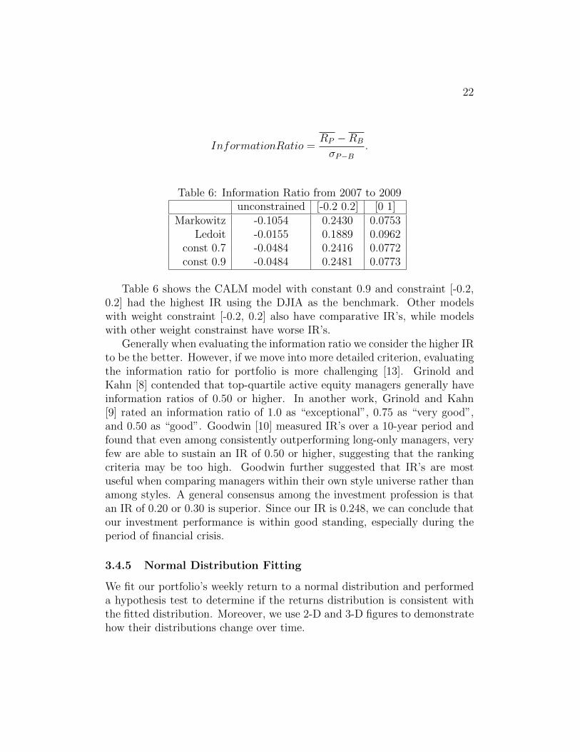
22

InformationRatio =RP −RB

σP−B.

Table 6: Information Ratio from 2007 to 2009unconstrained [-0.2 0.2] [0 1]

Markowitz -0.1054 0.2430 0.0753Ledoit -0.0155 0.1889 0.0962

const 0.7 -0.0484 0.2416 0.0772const 0.9 -0.0484 0.2481 0.0773

Table 6 shows the CALM model with constant 0.9 and constraint [-0.2,0.2] had the highest IR using the DJIA as the benchmark. Other modelswith weight constraint [-0.2, 0.2] also have comparative IR’s, while modelswith other weight constrainst have worse IR’s.

Generally when evaluating the information ratio we consider the higher IRto be the better. However, if we move into more detailed criterion, evaluatingthe information ratio for portfolio is more challenging [13]. Grinold andKahn [8] contended that top-quartile active equity managers generally haveinformation ratios of 0.50 or higher. In another work, Grinold and Kahn[9] rated an information ratio of 1.0 as “exceptional”, 0.75 as “very good”,and 0.50 as “good”. Goodwin [10] measured IR’s over a 10-year period andfound that even among consistently outperforming long-only managers, veryfew are able to sustain an IR of 0.50 or higher, suggesting that the rankingcriteria may be too high. Goodwin further suggested that IR’s are mostuseful when comparing managers within their own style universe rather thanamong styles. A general consensus among the investment profession is thatan IR of 0.20 or 0.30 is superior. Since our IR is 0.248, we can conclude thatour investment performance is within good standing, especially during theperiod of financial crisis.

3.4.5 Normal Distribution Fitting

We fit our portfolio’s weekly return to a normal distribution and performeda hypothesis test to determine if the returns distribution is consistent withthe fitted distribution. Moreover, we use 2-D and 3-D figures to demonstratehow their distributions change over time.

23

The hypothesis tests of Chi square goodness of fit test that we used todetermine whether or not our data fit a normal distribution is as follows:

• H0: Portfolio daily returns were taken from a normal distribution.

• H1: Portfolio daily returns were not taken from a normal distribution.

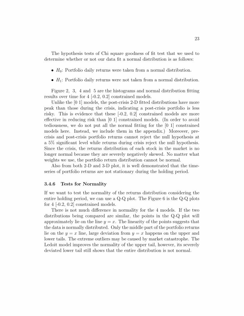
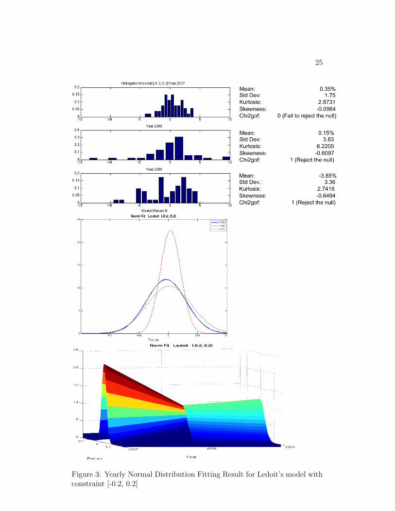
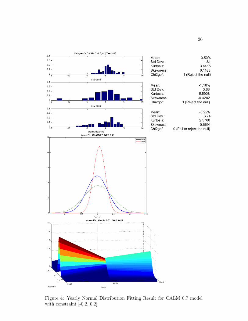
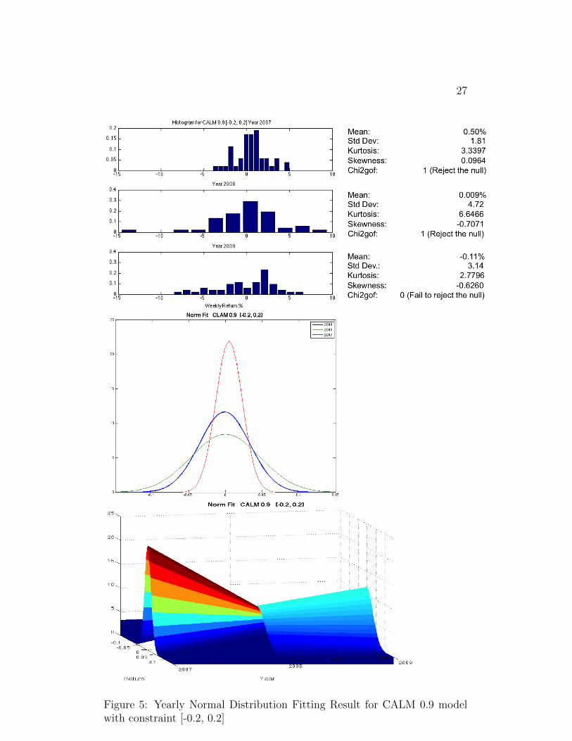
Figure 2, 3, 4 and 5 are the histograms and normal distribution fittingresults over time for 4 [-0.2, 0.2] constrained models.

Unlike the [0 1] models, the post-crisis 2-D fitted distributions have morepeak than those during the crisis, indicating a post-crisis portfolio is lessrisky. This is evidence that these [-0.2, 0.2] constrained models are moreeffective in reducing risk than [0 1] constrained models. (In order to avoidtediousness, we do not put all the normal fitting for the [0 1] constrainedmodels here. Instead, we include them in the appendix.) Moreover, pre-crisis and post-crisis portfolio returns cannot reject the null hypothesis ata 5% significant level while returns during crisis reject the null hypothesis.Since the crisis, the returns distribution of each stock in the market is nolonger normal because they are severely negatively skewed. No matter whatweights we use, the portfolio return distribution cannot be normal.

Also from both 2-D and 3-D plot, it is well demonstrated that the time-series of portfolio returns are not stationary during the holding period.

3.4.6 Tests for Normality

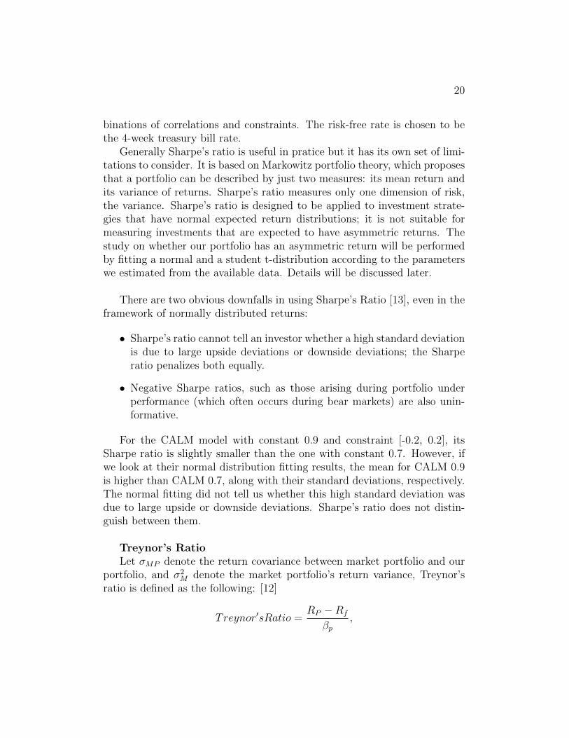
If we want to test the normality of the returns distribution considering theentire holding period, we can use a Q-Q plot. The Figure 6 is the Q-Q plotsfor 4 [-0.2, 0.2] constrained models.

There is not much difference in normality for the 4 models. If the twodistributions being compared are similar, the points in the Q-Q plot willapproximately lie on the line y = x. The linearity of the points suggests thatthe data is normally distributed. Only the middle part of the portfolio returnslie on the y = x line, large deviation from y = x happens on the upper andlower tails. The extreme outliers may be caused by market catastrophe. TheLedoit model improves the normality of the upper tail, however, its severelydeviated lower tail still shows that the entire distribution is not normal.

24

Figure 2: Yearly Normal Distribution Fitting Result for Markowitz modelwith constraint [-0.2, 0.2]

25

Figure 3: Yearly Normal Distribution Fitting Result for Ledoit’s model withconstraint [-0.2, 0.2]

26

Figure 4: Yearly Normal Distribution Fitting Result for CALM 0.7 modelwith constraint [-0.2, 0.2]

27

Figure 5: Yearly Normal Distribution Fitting Result for CALM 0.9 modelwith constraint [-0.2, 0.2]

28

−0.15 −0.1 −0.05 0 0.05 0.1Data

Normal Probability Plot Markowitz [−0.2, 0.2]

−0.1 −0.05 0 0.05Data

Normal Probability Plot Ledoit [−0.2, 0.2]

−0.1 −0.05 0 0.05 0.1Data

Normal Probability Plot CALM 0.7 [−0.2, 0.2]

−0.15 −0.1 −0.05 0 0.05 0.1Data

Normal Probability Plot CALM 0.9 [−0.2, 0.2]

Figure 6: Q-Q Plot for Four [-0.2, 0.2] Constrained Models

29

4 Conclusion

Our empirical analysis based on the portfolio performance from the financialcrisis from 2007 to 2009 indicates that incorporating forward-looking signalsinto covariance matrix estimation is an effective method to improve returnand reduce risk in market catastrophes.

Among the 12 combinations of models and constraints, Ledoit’s modeldoes not perform as well as the other 3 models as measured by Sharpe’s Ratio,holding period return, and weekly return and risk. CALM with constant0.7 and 0.9 performed similarly, indicating that the value of the constantnumber in a highly structured correlation matrix may not have a large impacton a portfolio’s performance. The standard Markowitz model performedmoderately well among these 4 models.

We found that [-0.2, 0.2] constrained models outperformed unconstrainedand [0 1] constrained models. Although their leverage ratios are higher andtake more risk than the [0 1] models, they obtain enough rewards, indicatingthat the excess risk is worth taking.

When the market is in a pre-crisis state, the standard Markowitz modelperformed the greatest. Since the market is calm before a crisis, the assump-tion that market behavior in the future is consistent with the past holds.If we include a highly structured correlation matrix, the covariance matrixoverestimates the market risk and thus the model instructs us to invest con-servatively and take less risk. As a result, the return is lower. However,during a post-crisis, the Ledoit model and CALM overcome the weaknessesof the Markowitz model and fairly measure the market risk. Thus they obtainbetter returns.

Should we decide to change investment models over time, Markowitz’model with constraint [-0.2, 0.2] works well during periods of relative ease.When market conditions worsen, we should switch to CALM 0.7 or CALM0.9 in order to achieve better results.

30

A Appendix

A.1 Matlab Code

The following is the core code computing the tangency weights for con-strained Ledoit’s Model and CALM.

[t,n]=size(data);

meanasset=mean(data);

data=data-meanasset(ones(t,1),:);

% compute sample covariance matrix

sample=(1/t).*(data’*data);

% compute prior

var=diag(sample);

sqrtvar=sqrt(var);

rBar=(sum(sum(sample./(sqrtvar(:,ones(n,1)).*sqrtvar(:,ones(n,1))’)))-n)...

/(n*(n-1));

prior=rBar*sqrtvar(:,ones(n,1)).*sqrtvar(:,ones(n,1))’;

prior(logical(eye(n)))=var;

%compute prior for CALM

%constant = 0.9;

%prior = constant*ones(n,n);

% what we call phi-hat

y=data.^2;

phiMat=y’*y/t - 2*(data’*data).*sample/t + sample.^2;

phi=sum(sum(phiMat));

% what we call rho-hat

term1=((data.^3)’*data)/t;

help = data’*data/t;

helpDiag=diag(help);

term2=helpDiag(:,ones(n,1)).*sample;

term3=help.*var(:,ones(n,1));

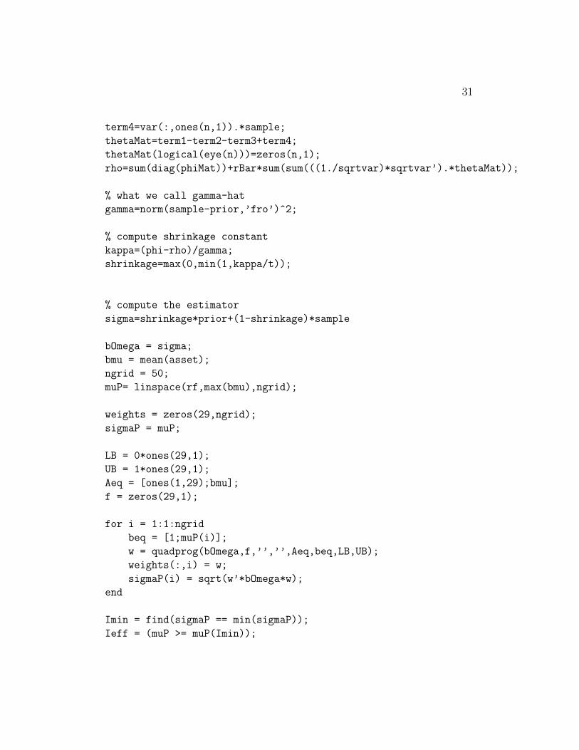
31

term4=var(:,ones(n,1)).*sample;

thetaMat=term1-term2-term3+term4;

thetaMat(logical(eye(n)))=zeros(n,1);

rho=sum(diag(phiMat))+rBar*sum(sum(((1./sqrtvar)*sqrtvar’).*thetaMat));

% what we call gamma-hat

gamma=norm(sample-prior,’fro’)^2;

% compute shrinkage constant

kappa=(phi-rho)/gamma;

shrinkage=max(0,min(1,kappa/t));

% compute the estimator

sigma=shrinkage*prior+(1-shrinkage)*sample

bOmega = sigma;

bmu = mean(asset);

ngrid = 50;

muP= linspace(rf,max(bmu),ngrid);

weights = zeros(29,ngrid);

sigmaP = muP;

LB = 0*ones(29,1);

UB = 1*ones(29,1);

Aeq = [ones(1,29);bmu];

f = zeros(29,1);

for i = 1:1:ngrid

beq = [1;muP(i)];

w = quadprog(bOmega,f,’’,’’,Aeq,beq,LB,UB);

weights(:,i) = w;

sigmaP(i) = sqrt(w’*bOmega*w);

end

Imin = find(sigmaP == min(sigmaP));

Ieff = (muP >= muP(Imin));

32

sharperatio = (muP-rf)./sigmaP;

Itangency = find(sharperatio == max(sharperatio));

weightsT=weights(:,Itangency)

ExpReturnT=bmu*weightsT;

VarT=weightsT’*bOmega*weightsT;

The following code fit the data with normal and run chi2gof test to testwhether the data were taken from a specific distribution.

netreturn7 = 100*netreturn7;

% fit the distribution of original data with normal dist.

pd_norm = fitdist(netreturn7,’Normal’)

[h,p] = chi2gof(netreturn7,’cdf’,pd_norm)

[f,x] = hist(netreturn7,15);

subplot(3,1,1)

% plot the percentage histogram

bar(x,f/sum(f));

title(’Histogram for CALM 0.9 [-0.2, 0.2] Year 2007’);

xlim([-15,10])

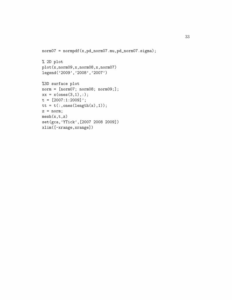
This code gives us the 2D and 3D surface plot of portfolio return.

xrange = 0.8;

x = [-xrange:.005:xrange];

% normal distribution fitting

return09 = xlsread(’DATA_DOW’,’weighted return’,’AF3:AF54’);

pd_norm09 = fitdist(return09,’Normal’);

norm09 = normpdf(x,pd_norm09.mu,pd_norm09.sigma);

return08 = xlsread(’DATA_DOW’,’weighted return’,’AF56:AF107’);

pd_norm08 = fitdist(return08,’Normal’);

norm08 = normpdf(x,pd_norm08.mu,pd_norm08.sigma);

return07 = xlsread(’DATA_DOW’,’weighted return’,’AF109:AF161’);

pd_norm07 = fitdist(return07,’Normal’);

33

norm07 = normpdf(x,pd_norm07.mu,pd_norm07.sigma);

% 2D plot

plot(x,norm09,x,norm08,x,norm07)

legend(’2009’,’2008’,’2007’)

%3D surface plot

norm = [norm07; norm08; norm09;];

xx = x(ones(3,1),:);

t = [2007:1:2009]’;

tt = t(:,ones(length(x),1));

z = norm;

mesh(x,t,z)

set(gca,’YTick’,[2007 2008 2009])

xlim([-xrange,xrange])

34

References

[1] O. Ledoit & M. Wolf, Honey, “Honey, I Shrunk the Sample CovarianceMatrix,” The Journal of Portfolio Management, 30.4 (2004), pp. 110-119.

[2] T. S. Ahluwalia, R. P. Hark, D. R. Helkey, N.F. Marshall, M. S. Blais,C. Morales, “Incorporating Forward-Looking Signals into CovarianceMatrix Estimation for Portfolio Optimization,” REU Project, 2012.

[3] D. Kennett, M. Raddant, T. Lux, and E. Ben-Jacob, “Evolvement ofUniformity and Volatility in the Stressed Global Financial Village.”PLoS ONE Journal, 7.2 (2012), pp. 1-14.

[4] T. Bollerslv, “Modelling the Coherence in Short-Run Nominal ExchangeRates: A Multivariate Generalized ARCH Model.” Review of Economicsand Statistics, 72.3 (1990), pp. 498-505.

[5] R. Engles, “IDynamic Conditional Correlation: A Simple Class of Multi-variate Generalized Autoregressive Conditional Heteroskedasticity Mod-els.” Journal of Business & Economic Statistics, 20.3 (2012), pp. 339-350.

[6] Vaart, A. W. van der, “Asymptotic Statistics.” Cambridge, UK ; NewYork, NY, USA : Cambridge University Press, 1998

[7] H. Markowitz, “Portfolio Selection.” The Journal of Finance, 7.1 (1952),pp. 77-91.

[8] R. C. Grinold, R. N. Kahn, “Active Portfolio Management.” Review ofFinancial Studies, ISSN 0893-9454, 10/2000, Volume 13, Issue 4, pp.1153-1156.

[9] R. C. Grinold, R. N. Kahn, “Active Portfolio Management.” Chicago,IL: Richard D. Irwin. (1995).

[10] T. H. Goodwin, “The Information Ratio.”, In Investment PerformanceMeasurement: Evaluation and Presenting Results (2009). Edited byPhilip Lawton and Todd Jankowski. Hoboken, NJ: John Wiley &Sons:705-718. Reprinted from Financial Analysts Journal, vol. 54, no. 4(July/August 1998):34-43.

35

[11] Federal Reserve, “Selected Interest Rates (Weekly)-H.15.”http://www.federalreserve.gov/releases/h15/

[12] D. Ruppert, Ronald N. Kahn, “Statistics and Finance: An Introduc-tion.” G. Casella, S. Fienberg, and I. Olkin, eds., Springer Science &Business Media, New York, NY, 2006, pp. 75-326.

[13] D. Kidd, “The Sharpe Ratio and the Information Ratio.” InvestmentPerformance Measurement Feature Articles July 2011, Vol. 2011, No.1-4 pages, CFA Institute