8/8/2019 Jack Markowitz

http://slidepdf.com/reader/full/jack-markowitz 1/13

ASSIGNMENT

ON

HARRY MARKOWITZ MODEL THEORY

GURU GOBIND SINGS INDRAPARASTHA

UNIVERSITY

KASMERI GATE,DELHI:-6

Submitted to:- Submitted by:-

Prof:-K.L. Dhaiya Jagarnath shah

Roll no:-062

MBA(weekend),Gen

8/8/2019 Jack Markowitz

http://slidepdf.com/reader/full/jack-markowitz 2/13

Modern portfolio theoryModern portfolio theory (MPT) is a theory of investment which attempts to maximize

 portfolio expected return for a given amount of portfolio risk, or equivalently minimize

risk for a given level of expected return, by carefully choosing the proportions of variousassets. Although MPT is widely used in practice in the financial industry and several of 

its creators won a Nobel prize for the theory, in recent years the basic assumptions of 

MPT have been widely challenged by fields such as behavioral economics.

MPT is a mathematical formulation of the concept of diversification in investing, with the

aim of selecting a collection of investment assets that has collectively lower risk than any

individual asset. That this is possible can be seen intuitively because different types of assets often change in value in opposite ways. For example, when prices in the stock 

market fall, prices in the bond market often increase, and vice versa[citation needed ]. A

collection of both types of assets can therefore have lower overall risk than either individually. But diversification lowers risk even if assets' returns are not negatively

correlated—indeed, even if they are positively correlated.

More technically, MPT models an asset's return as a normally distributed (or more

generally as an elliptically distributed random variable), defines risk as the standard

deviation of return, and models a portfolio as a weighted combination of assets so that the

return of a portfolio is the weighted combination of the assets' returns. By combiningdifferent assets whose returns are not perfectly positively correlated, MPT seeks to

reduce the total variance of the portfolio return. MPT also assumes that investors are

rational and markets are efficient.

MPT was developed in the 1950s through the early 1970s and was considered an

important advance in the mathematical modeling of finance. Since then, many theoreticaland practical criticisms have been leveled against it. These include the fact that financial

returns do not follow a Gaussian distribution or indeed any symmetric distribution, and

that correlations between asset classes are not fixed but can vary depending on externalevents (especially in crises). Further, there is growing evidence that investors are not

rational and markets are not efficient.

Concept

The fundamental concept behind MPT is that the assets in an investment portfolio cannot

 be selected individually, each on their own merits. Rather, it is important to consider howeach asset changes in price relative to how every other asset in the portfolio changes in

 price.

Investing is a tradeoff between risk and expected return. In general, assets with higher 

expected returns are riskier. For a given amount of risk, MPT describes how to select a

 portfolio with the highest possible expected return. Or, for a given expected return, MPTexplains how to select a portfolio with the lowest possible risk (the targeted expected

return cannot be more than the highest-returning available security, of course, unless

negative holdings of assets are possible.)[3]

8/8/2019 Jack Markowitz

http://slidepdf.com/reader/full/jack-markowitz 3/13

MPT is therefore a form of diversification. Under certain assumptions and for specific

quantitative definitions of risk and return, MPT explains how to find the best possible

diversification strategy.

History

Harry Markowitz introduced MPT in a 1952 article[4] and a 1959 book.[5] See also[3].

Mathematical model

In some sense the mathematical derivation below is MPT, although the basic concepts

 behind the model have also been very influential.[3]

This section develops the "classic" MPT model. There have been many extensions since.

Risk and expected return

MPT assumes that investors are risk averse, meaning that given two portfolios that offer the same expected return, investors will prefer the less risky one. Thus, an investor willtake on increased risk only if compensated by higher expected returns. Conversely, an

investor who wants higher expected returns must accept more risk. The exact trade-off 

will be the same for all investors, but different investors will evaluate the trade-off differently based on individual risk aversion characteristics. The implication is that a

rational investor will not invest in a portfolio if a second portfolio exists with a more

favorable risk-expected return profile – i.e., if for that level of risk an alternative portfolio

exists which has better expected returns.

 Note that the theory uses standard deviation of return as a proxy for risk. There are

 problems with this, however; see criticism.

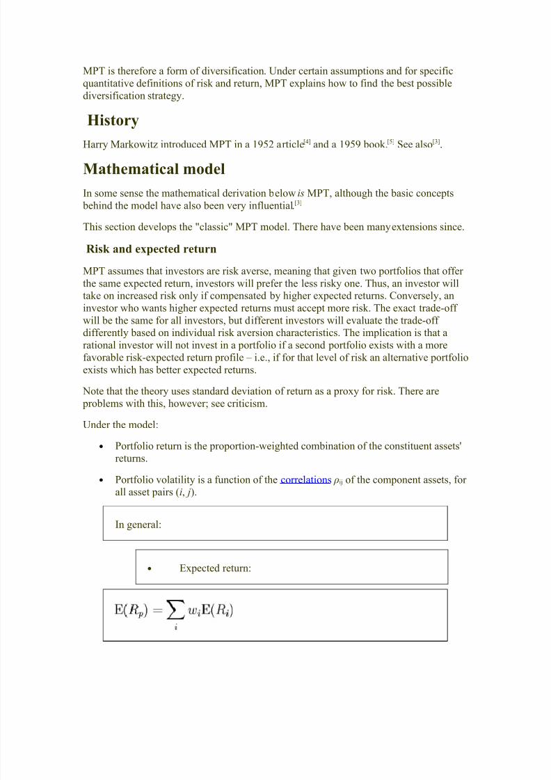
Under the model:

• Portfolio return is the proportion-weighted combination of the constituent assets'

returns.

• Portfolio volatility is a function of the correlations  ρij of the component assets, for all asset pairs (i, j).

In general:

• Expected return:

8/8/2019 Jack Markowitz

http://slidepdf.com/reader/full/jack-markowitz 4/13

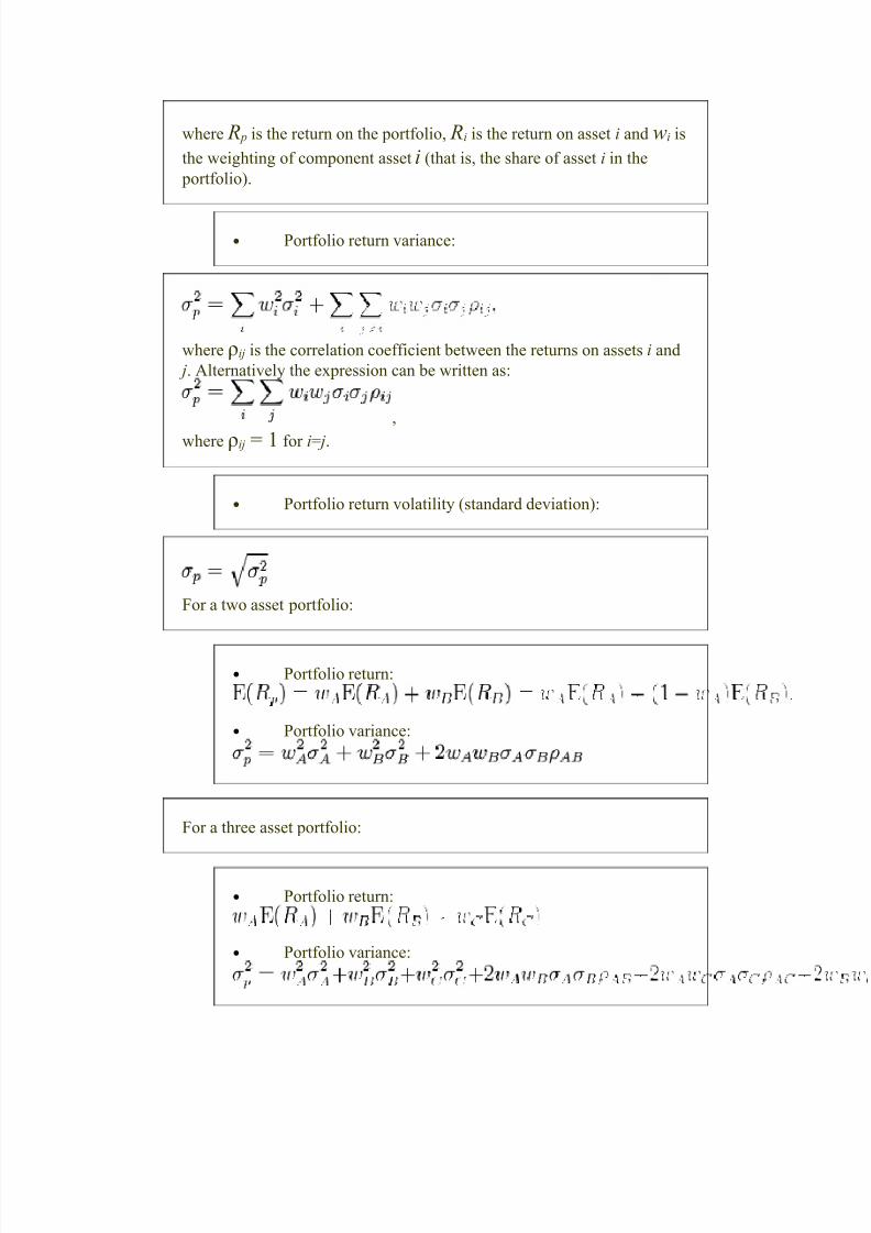
where R p is the return on the portfolio, Ri is the return on asset i and wi is

the weighting of component asset i (that is, the share of asset i in the

 portfolio).

• Portfolio return variance:

where ρij is the correlation coefficient between the returns on assets i and

 j. Alternatively the expression can be written as:

,

where ρij = 1 for i= j.

• Portfolio return volatility (standard deviation):

For a two asset portfolio:

• Portfolio return:

• Portfolio variance:

For a three asset portfolio:

• Portfolio return:

• Portfolio variance:

8/8/2019 Jack Markowitz

http://slidepdf.com/reader/full/jack-markowitz 5/13

Diversification

An investor can reduce portfolio risk simply by holding combinations of instruments

which are not perfectly positively correlated (correlation coefficient )).In other words, investors can reduce their exposure to individual asset risk by holding a

diversified portfolio of assets. Diversification may allow for the same portfolio expectedreturn with reduced risk.

If all the asset pairs have correlations of 0—they are perfectly uncorrelated—the

 portfolio's return variance is the sum over all assets of the square of the fraction held inthe asset times the asset's return variance (and the portfolio standard deviation is the

square root of this sum).

The efficient frontier with no risk-free asset

Efficient Frontier. The hyperbola is sometimes referred to as the 'Markowitz Bullet', andis the efficient frontier if no risk-free asset is available.

As shown in this graph, every possible combination of the risky assets, without including

any holdings of the risk-free asset, can be plotted in risk-expected return space, and the

collection of all such possible portfolios defines a region in this space. The left boundaryof this region is a hyperbola,[6] and the upper edge of this region is the efficient frontier in

the absence of a risk-free asset (sometimes called "the Markowitz bullet"). Combinations

along this upper edge represent portfolios (including no holdings of the risk-free asset)for which there is lowest risk for a given level of expected return. Equivalently, a

 portfolio lying on the efficient frontier represents the combination offering the best

 possible expected return for given risk level.

Matrices are preferred for calculations of the efficient frontier. In matrix

form, for a given "risk tolerance" , the efficient frontier is

found by minimizing the following expression:

wT Σw − q * RT w

8/8/2019 Jack Markowitz

http://slidepdf.com/reader/full/jack-markowitz 6/13

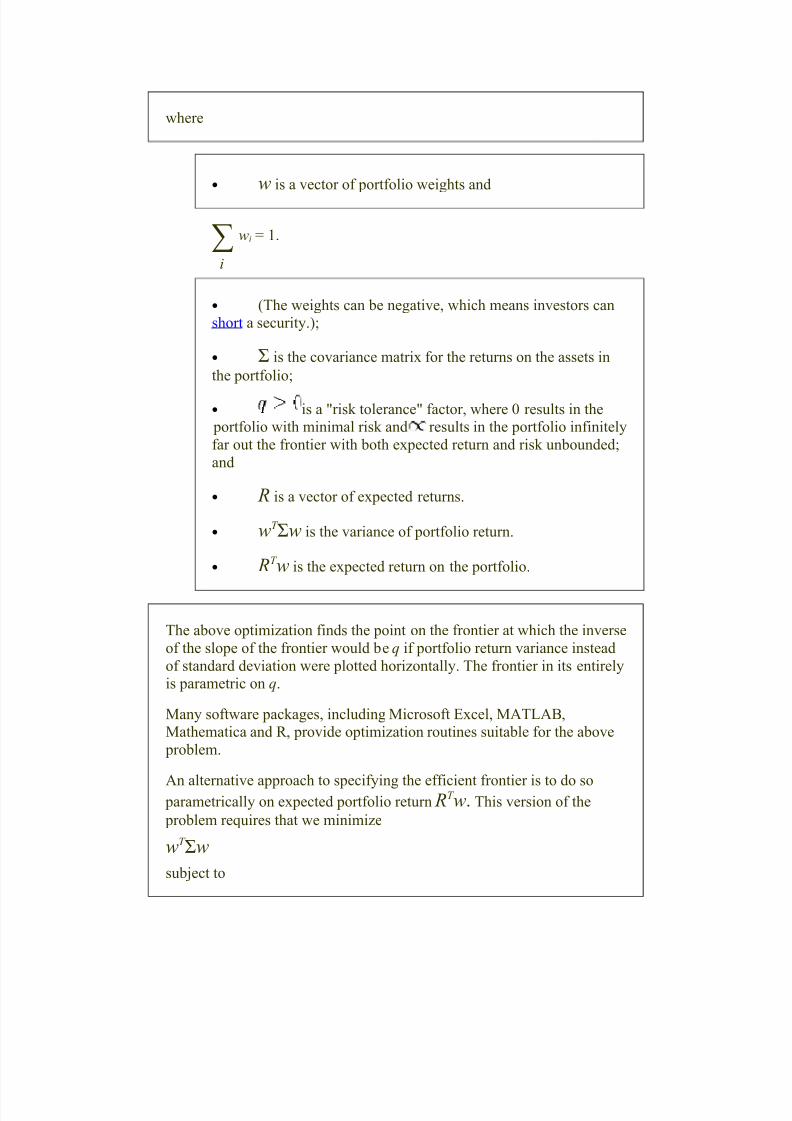
where

• w is a vector of portfolio weights and

∑ wi = 1.

i

• (The weights can be negative, which means investors canshort a security.);

• Σ is the covariance matrix for the returns on the assets in

the portfolio;

• is a "risk tolerance" factor, where 0 results in the portfolio with minimal risk and results in the portfolio infinitely

far out the frontier with both expected return and risk unbounded;

and

• R is a vector of expected returns.

• wT Σw is the variance of portfolio return.

• RT w is the expected return on the portfolio.

The above optimization finds the point on the frontier at which the inverse

of the slope of the frontier would be q if portfolio return variance instead

of standard deviation were plotted horizontally. The frontier in its entirelyis parametric on q.

Many software packages, including Microsoft Excel, MATLAB,Mathematica and R , provide optimization routines suitable for the above

 problem.

An alternative approach to specifying the efficient frontier is to do so parametrically on expected portfolio return RT w. This version of the

 problem requires that we minimize

wT Σw

subject to

8/8/2019 Jack Markowitz

http://slidepdf.com/reader/full/jack-markowitz 7/13

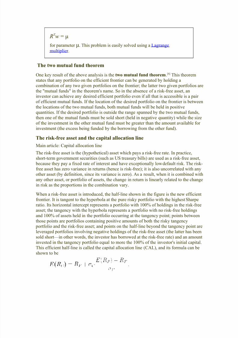
 RT w = μ

for parameter μ. This problem is easily solved using a Lagrange

multiplier .

The two mutual fund theorem

One key result of the above analysis is the two mutual fund theorem.[6] This theoremstates that any portfolio on the efficient frontier can be generated by holding a

combination of any two given portfolios on the frontier; the latter two given portfolios are

the "mutual funds" in the theorem's name. So in the absence of a risk-free asset, aninvestor can achieve any desired efficient portfolio even if all that is accessible is a pair 

of efficient mutual funds. If the location of the desired portfolio on the frontier is between

the locations of the two mutual funds, both mutual funds will be held in positivequantities. If the desired portfolio is outside the range spanned by the two mutual funds,

then one of the mutual funds must be sold short (held in negative quantity) while the sizeof the investment in the other mutual fund must be greater than the amount available for 

investment (the excess being funded by the borrowing from the other fund).

The risk-free asset and the capital allocation line

Main article: Capital allocation line

The risk-free asset is the (hypothetical) asset which pays a risk-free rate. In practice,short-term government securities (such as US treasury bills) are used as a risk-free asset,

 because they pay a fixed rate of interest and have exceptionally low default risk. The risk-

free asset has zero variance in returns (hence is risk-free); it is also uncorrelated with anyother asset (by definition, since its variance is zero). As a result, when it is combined with

any other asset, or portfolio of assets, the change in return is linearly related to the change

in risk as the proportions in the combination vary.

When a risk-free asset is introduced, the half-line shown in the figure is the new efficient

frontier. It is tangent to the hyperbola at the pure risky portfolio with the highest Sharpe

ratio. Its horizontal intercept represents a portfolio with 100% of holdings in the risk-freeasset; the tangency with the hyperbola represents a portfolio with no risk-free holdings

and 100% of assets held in the portfolio occurring at the tangency point; points between

those points are portfolios containing positive amounts of both the risky tangency portfolio and the risk-free asset; and points on the half-line beyond the tangency point are

leveraged portfolios involving negative holdings of the risk-free asset (the latter has been

sold short—in other words, the investor has borrowed at the risk-free rate) and an amountinvested in the tangency portfolio equal to more the 100% of the investor's initial capital.

This efficient half-line is called the capital allocation line (CAL), and its formula can be

shown to be

8/8/2019 Jack Markowitz

http://slidepdf.com/reader/full/jack-markowitz 8/13

In this formula P is the sub-portfolio of risky assets at the tangency with the Markowitz

 bullet, F is the risk-free asset, and C is a combination of portfolios P and F .

By the diagram, the introduction of the risk-free asset as a possible component of the

 portfolio has improved the range of risk-expected return combinations available, because

everywhere except at the tangency portfolio the half-line gives a higher expected returnthan the hyperbola does at every possible risk level. The fact that all points on the linear 

efficient locus can be achieved by a combination of holdings of the risk-free asset and the

tangency portfolio is known as the one mutual fund theorem,[6] where the mutual fundreferred to is the tangency portfolio.

Asset pricing using MPT

The above analysis describes optimal behavior of an individual investor. Asset pricing

theory builds on this analysis in the following way. Since everyone holds the risky assets

in identical proportions to each other—namely in the proportions given by the tangency portfolio—in market equilibrium the risky assets' prices, and therefore their expected

returns, will adjust so that the ratios in the tangecy portfolio are the same as the ratios inwhich the risky assets are supplied to the market. Thus relative supplies will equalrelative demands. MPT derives the required expected return for a correctly priced asset in

this context.

Systematic risk and specific risk 

Specific risk is the risk associated with individual assets - within a portfolio these risks

can be reduced through diversification (specific risks "cancel out"). Specific risk is alsocalled diversifiable, unique, unsystematic, or idiosyncratic risk. Systematic risk (a.k.a.

 portfolio risk or market risk) refers to the risk common to all securities - except for 

selling short as noted below, systematic risk cannot be diversified away (within onemarket). Within the market portfolio, asset specific risk will be diversified away to theextent possible. Systematic risk is therefore equated with the risk (standard deviation) of 

the market portfolio.

Since a security will be purchased only if it improves the risk-expected return

characteristics of the market portfolio, the relevant measure of the risk of a security is the

risk it adds to the market portfolio, and not its risk in isolation. In this context, thevolatility of the asset, and its correlation with the market portfolio, are historically

observed and are therefore given. (There are several approaches to asset pricing that

attempt to price assets by modelling the stochastic properties of the moments of assets'returns - these are broadly referred to as conditional asset pricing models.)

Systematic risks within one market can be managed through a strategy of using both long

and short positions within one portfolio, creating a "market neutral" portfolio.

Capital asset pricing model

Main article: Capital Asset Pricing Model

8/8/2019 Jack Markowitz

http://slidepdf.com/reader/full/jack-markowitz 9/13

The asset return depends on the amount paid for the asset today. The price paid must

ensure that the market portfolio's risk / return characteristics improve when the asset is

added to it. The CAPM is a model which derives the theoretical required expected return(i.e., discount rate) for an asset in a market, given the risk-free rate available to investors

and the risk of the market as a whole. The CAPM is usually expressed:

• β, Beta, is the measure of asset sensitivity to a movement in the overall market;

Beta is usually found via regression on historical data. Betas exceeding onesignify more than average "riskiness" in the sense of the asset's contribution to

overall portfolio risk; betas below one indicate a lower than average risk 

contribution.

• is the market premium, the expected excess return of the

market portfolio's expected return over the risk-free rate.

This equation can be statistically estimated using the following regression equation:

where αi is called the asset's alpha , βi is the asset's beta coefficient and SCL is the

Securities Characteristics Line.

Once an asset's expected return, E ( Ri), is calculated using CAPM, the future cash flows 

of the asset can be discounted to their  present value using this rate to establish the correct

 price for the asset. A riskier stock will have a higher beta and will be discounted at ahigher rate; less sensitive stocks will have lower betas and be discounted at a lower rate.

In theory, an asset is correctly priced when its observed price is the same as its value

calculated using the CAPM derived discount rate. If the observed price is higher than thevaluation, then the asset is overvalued; it is undervalued for a too low price.

(1) The incremental impact on risk and expected return when an additional

risky asset, a, is added to the market portfolio, m, follows from theformulae for a two-asset portfolio. These results are used to derive the

asset-appropriate discount rate.

Market portfolio's risk =

Hence, risk added to portfolio =

 but since the weight of the asset will be relatively low,

i.e. additional risk =

Market portfolio's expected return =

Hence additional expected return =

8/8/2019 Jack Markowitz

http://slidepdf.com/reader/full/jack-markowitz 10/13

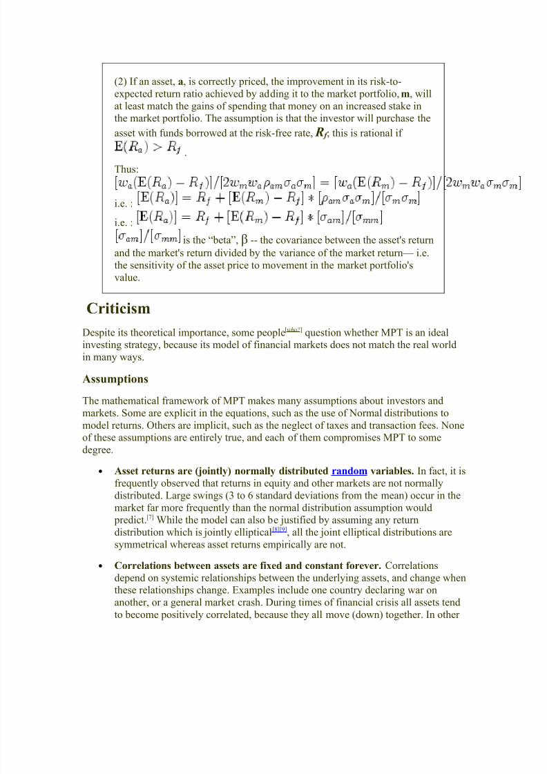
(2) If an asset, a, is correctly priced, the improvement in its risk-to-

expected return ratio achieved by adding it to the market portfolio, m, will

at least match the gains of spending that money on an increased stake inthe market portfolio. The assumption is that the investor will purchase the

asset with funds borrowed at the risk-free rate, R f  ; this is rational if 

.

Thus:

i.e. :

i.e. :

is the “beta”, β -- the covariance between the asset's return

and the market's return divided by the variance of the market return— i.e.

the sensitivity of the asset price to movement in the market portfolio's

value.

Criticism

Despite its theoretical importance, some people[who?] question whether MPT is an idealinvesting strategy, because its model of financial markets does not match the real world

in many ways.

Assumptions

The mathematical framework of MPT makes many assumptions about investors and

markets. Some are explicit in the equations, such as the use of Normal distributions to

model returns. Others are implicit, such as the neglect of taxes and transaction fees. Noneof these assumptions are entirely true, and each of them compromises MPT to some

degree.

• Asset returns are (jointly) normally distributed random variables. In fact, it isfrequently observed that returns in equity and other markets are not normally

distributed. Large swings (3 to 6 standard deviations from the mean) occur in the

market far more frequently than the normal distribution assumption would predict.[7] While the model can also be justified by assuming any return

distribution which is jointly elliptical[8][9], all the joint elliptical distributions are

symmetrical whereas asset returns empirically are not.

• Correlations between assets are fixed and constant forever. Correlations

depend on systemic relationships between the underlying assets, and change whenthese relationships change. Examples include one country declaring war on

another, or a general market crash. During times of financial crisis all assets tend

to become positively correlated, because they all move (down) together. In other 

8/8/2019 Jack Markowitz

http://slidepdf.com/reader/full/jack-markowitz 11/13

words, MPT breaks down precisely when investors are most in need of protection

from risk.

• All investors aim to maximize economic utility (in other words, to make as

much money as possible, regardless of any other considerations). This is a key

assumption of the efficient market hypothesis, upon which MPT relies.

• All investors are rational and risk-averse. This is another assumption of the

efficient market hypothesis, but we now know from behavioral economics thatmarket participants are not rational. It does not allow for "herd behavior" or 

investors who will accept lower returns for higher risk. Casino gamblers clearly

 pay for risk, and it is possible that some stock traders will pay for risk as well.

• All investors have access to the same information at the same time. This also

comes from the efficient market hypothesis. In fact, real markets contain

information asymmetry, insider trading, and those who are simply better informedthan others.

• Investors have an accurate conception of possible returns, i.e., the probability

beliefs of investors match the true distribution of returns. A different

 possibility is that investors' expectations are biased, causing market prices to be

informationally inefficient. This possibility is studied in the field of  behavioral

finance, which uses psychological assumptions to provide alternatives to theCAPM such as the overconfidence-based asset pricing model of Kent Daniel,

David Hirshleifer, and Avanidhar Subrahmanyam (2001).[10]

• There are no taxes or transaction costs. Real financial products are subject both

to taxes and transaction costs (such as broker fees), and taking these into account

will alter the composition of the optimum portfolio. These assumptions can be

relaxed with more complicated versions of the model.[citation needed ]

• All investors are price takers, i.e., their actions do not influence prices. Inreality, sufficiently large sales or purchases of individual assets can shift market

 prices for that asset and others (via cross-elasticity of demand.) An investor may

not even be able to assemble the theoretically optimal portfolio if the market

moves too much while they are buying the required securities.

• Any investor can lend and borrow an unlimited amount at the risk free rate

of interest. In reality, every investor has a credit limit.

• All securities can be divided into parcels of any size. In reality, fractional

shares usually cannot be bought or sold, and some assets have minimum orderssizes.

More complex versions of MPT can take into account a more sophisticated model of the

world (such as one with non-normal distributions and taxes) but all mathematical modelsof finance still rely on many unrealistic premises.

MPT does not really model the market

8/8/2019 Jack Markowitz

http://slidepdf.com/reader/full/jack-markowitz 12/13

The risk, return, and correlation measures used by MPT are based on expected values, 

which means that they are mathematical statements about the future (the expected value

of returns is explicit in the above equations, and implicit in the definitions of variance andcovariance.) In practice investors must substitute predictions based on historical

measurements of asset return and volatility for these values in the equations. Very often

such expected values fail to take account of new circumstances which did not exist whenthe historical data were generated.

More fundamentally, investors are stuck with estimating key parameters from past marketdata because MPT attempts to model risk in terms of the likelihood of losses, but says

nothing about why those losses might occur. The risk measurements used are

 probabilistic in nature, not structural. This is a major difference as compared to many

engineering approaches to risk management.

Options theory and MPT have at least one important conceptual difference

from the probabilistic risk assessment done by nuclear power [plants]. APRA is what economists would call a structural model . The components

of a system and their relationships are modeled in Monte Carlosimulations. If valve X fails, it causes a loss of back pressure on pump Y,causing a drop in flow to vessel Z, and so on.

But in the Black-Scholes equation and MPT, there is no attempt to explain

an underlying structure to price changes. Various outcomes are simplygiven probabilities. And, unlike the PRA, if there is no history of a

 particular system-level event like a liquidity crisis, there is no way to

compute the odds of it. If nuclear engineers ran risk management this way,they would never be able to compute the odds of a meltdown at a

 particular plant until several similar events occurred in the same reactor 

design. —Douglas W. Hubbard, 'The Failure of Risk Management', p. 67, John

Wiley & Sons, 2009. ISBN 978-0-470-38795-5

Essentially, the mathematics of MPT view the markets as a collection of dice. By

examining past market data we can develop hypotheses about how the dice are weighted,

 but this isn't helpful if the markets are actually dependent upon a much bigger and morecomplicated chaotic system -- the world. For this reason, accurate structural models of 

real financial markets are unlikely to be forthcoming because they would essentially be

structural models of the entire world. Nonetheless there is growing awareness of the

concept of systemic risk in financial markets, which should lead to more sophisticated

market models.

Mathematical risk measurements are also useful only to the degree that they reflectinvestors' true concerns -- there is no point minimizing a variable that nobody cares about

in practice. MPT uses the mathematical concept of variance to quantify risk, and this

might be justified under the assumption of elliptically distributed returns such asnormally distributed returns, but for general return distributions other risk measures (like

coherent risk measures) might better reflect investors' true preferences.

8/8/2019 Jack Markowitz

http://slidepdf.com/reader/full/jack-markowitz 13/13

In particular, variance is a symmetric measure that counts abnormally high returns as just

as risky as abnormally low returns. Some would argue that, in reality, investors are only

concerned about losses, and do not care about the dispersion or tightness of above-average returns. According to this view, our intuitive concept of risk is fundamentally

asymmetric in nature.

MPT does not account for the social, environmental, strategic, or personal dimensions of 

investment decisions. It only attempts to maximize risk-adjusted returns, without regard

to other consequences. In a narrow sense, its complete reliance on asset prices makes itvulnerable to all the standard market failures such as those arising from information

asymmetry, externalities, and public goods. It also rewards corporate fraud and dishonest

accounting. More broadly, a firm may have strategic or social goals that shape its

investment decisions, and an individual investor might have personal goals. In either case, information other than historical returns is relevant.

See also socially-responsible investing, fundamental analysis.

ExtensionsSince MPT's introduction in 1952, many attempts have been made to improve the model,

especially by using more realistic assumptions.

Post-modern portfolio theory extends MPT by adopting non-normally distributed,

asymmetric measures of risk. This helps with some of these problems, but not others.

Black-Litterman model optimization is an extension of unconstrained Markowitz

optimization which incorporates relative and absolute `views' on inputs of risk and

returns.

 

Comparison with arbitrage pricing theory

The SML and CAPM are often contrasted with the arbitrage pricing theory (APT), which

holds that the expected return of a financial asset can be modeled as a linear function of various macro-economic factors, where sensitivity to changes in each factor is

represented by a factor specific beta coefficient.

The APT is less restrictive in its assumptions: it allows for an explanatory (as opposed to

statistical) model of asset returns, and assumes that each investor will hold a unique

 portfolio with its own particular array of betas, as opposed to the identical "market portfolio". Unlike the CAPM, the APT, however, does not itself reveal the identity of its

 priced factors - the number and nature of these factors is likely to change over time and

 between economies.