Clustering of Rainfall Distribution Patterns in Peninsular ...

Malaysian Journal of Science 38 (Special Issue 2): 84 - 99 (2019)

THE INTERNATIONAL SEMINAR ON MATHEMATICS IN INDUSTRY (ISMI)

AND THE INTERNATIONAL CONFERENCE ON THEORETICAL AND APPLIED STATISTICS (ICTAS)

ISMI-ICTAS18 [4-6 SEPTEMBER 2018]

84

Clustering of Rainfall Distribution Patterns in Peninsular Malaysia using Time

Series Clustering Method

Noratiqah Mohd Ariff1a, Mohd Aftar Abu Bakar1b*, Sharifah Faridah Syed Mahbar2c, Mohd

Shahrul Mohd Nadzir3,4d

1 School of Mathematical Sciences, Faculty of Science and Technology, Universiti Kebangsaan Malaysia, 43600 UKM

Bangi, Selangor, MALAYSIA. E-mail: [email protected]; [email protected]

2 Pusat Operasi Cuaca & Geofizik Nasional, Jabatan Meteorologi Malaysia, Kementerian Tenaga, Sains, Teknologi,

Alam Sekitar & Perubahan Iklim, Jalan Sultan, 46667 Petaling Jaya, Selangor, MALAYSIA. E-mail:

[email protected]

3 School of Environmental and Natural Resource Sciences, Faculty of Science and Technology, Universiti Kebangsaan

Malaysia, 43600, UKM Bangi, Selangor, MALAYSIA. 4 Centre for Tropical Climate Change System, Institute of Climate Change, Universiti Kebangsaan Malaysia, 43600,

UKM Bangi, Selangor, MALAYSIA. E-mail: [email protected]

* Corresponding Author: [email protected]

Received: 21st April 2019 Revised: 6th August 2019 Published: 30th September 2019

DOI : https://doi.org/10.22452/mjs.sp2019no2.8

ABSTRACT Time series clustering technique was used in this study to categorize the

locations in Peninsular Malaysia according to the similarity of rainfall distribution patterns. Daily

rainfall time series data from 12 meteorological observation stations across Peninsular Malaysia

have been considered for this study. Four dissimilarity measure methods were examined and

compared in terms of accuracy and suitability, namely Euclidean distance (ED), complexity-

invariant distance (CID), correlation-based distance (COR) and integrated periodogram-based

distance (IP). The average silhouette width (ASW) was used to determine the optimal group number

for the rainfall time series data. Using Ward’s hierarchical clustering method, this study found that

the rainfall time series in Peninsular Malaysia can be divided into four regions of homogeneous

climate zones. Based on the results, the IP was the most suitable dissimilarity measures for

clustering rainfall time series data in Peninsular Malaysia, except during the Southwest Monsoon

where the COR performed better.

Keywords: time series clustering, dissimilarity measures, rainfall patterns, Peninsular Malaysia.

1. INTRODUCTION

Accuracy in weather forecasting helps

to contribute to the nation socioeconomic

activities and development. The weather

reports are used in planning and decision

making for matters related to disaster

management, water management, agriculture,

industry and tourism. Clustering technique is

one of the effective data mining techniques to

extract useful information. It is important to

identify the set of objects whose class is

unknown in data mining. This has been

applied in the study of taxonomy, agriculture,

remote sensing and process control (Kavitha

& Punithavalli, 2010), as well as meteorology

study to determine and classify rainfall

patterns (Munoz-Diaz & Rodrigo, 2004;

Soltani & Modarres, 2006).

Time series clustering is a technique

which can partition time series data into

groups based on its similarity or distance.

Time series clustering has been used for

recognizing dynamic changes in time series,

discovering patterns, prediction and





85

recommendation in many field of studies such

as in climate, energy, environment, finance

and medicine (Aghabozorgi et al., 2015; Rani

& Sikka, 2012). Ahmad et al. (2013) used the

hierarchical clustering approach to regionalise

the daily rainfall data in Peninsular Malaysia.

However, they do not consider the seasonal

factor, which is crucial for the Malaysian

climate. This was conducted by clustering the

time series data only during the Northeast

Monsoon (or Southwest Monsoon), instead of

clustering the whole time series.

In this study, the rainfall time series

data from 12 meteorological stations in

Peninsular Malaysia from 1970 to 2014 (45

years) were analysed using clustering

technique. This study examined and

compared four dissimilarity measure methods

used to cluster the rainfall time series in

Malaysia according to homogenous climate

zone.

2. RAINFALL DATA

Malaysia is a country located near to

the equator, divided into two regions which

are the Peninsular Malaysia and East

Malaysia separated by the South China Sea.

The climate is hot and humid throughout the

year with heavy rainfalls. There are two

monsoon seasons, the Southwest Monsoon

(May to August), where the east coast of

Peninsular Malaysia, west of Sarawak and

east coast of Sabah have more rainfalls, and

the Northeast Monsoon (November to

February), where the rainfall occurrence is

lesser at the east coast of Peninsular

Malaysia. The total precipitation is between

2000 and 4000 mm annually.

Twelve Malaysian Meteorological

Department (MMD) observation stations that

cover three zones in Peninsular Malaysia

were selected in this study. Details for each

station and its location is depicted in Table 1

and Figure 1. The daily time series rainfall

data from 1970 until 2014 were used in this

analysis.

Table 1: Stations details, location and percentage of missing data for each station.

Station Station

Code

Latitude

(°N)

Longitude

(°E)

Mean Sea

Level

(MSL)

(m)

Missing

Data

(%)

Alor Setar 48603 6.2 100.4 3.9 -

Bayan Lepas 48601 5.3 100.2667 2.5 -

Kota Bharu 48615 6.1667 102.3 4.4 -

Hospital Dungun 49476 4.7667 103.4167 3 2.46

Kuantan 48657 3.7667 103.2167 15.2 -

Mersing 48674 2.45 103.8333 43.6 -

Subang 48647 3.1333 101.55 16.6 -

Malacca 48665 2.2667 102.25 8.5 -

Hospital Baling 41545 5.6833 100.9167 52 0.42

Ipoh 48625 4.5667 101.1 40.1 -

Hospital Tapah 43421 4.2 101.2667 35 0.27

Sitiawan 48620 4.2167 100.7 6.8 -





86

Figure 1: Locations of rain gauge stations.

3. TIME SERIES CLUSTER

ANALYSIS

Cluster analysis is a technique that

groups certain observations with similar

characteristics or traits when the true group is

unknown. Cluster analysis is applied in

various data types, for example numerical

data (Michinaka et al., 2011), image data

(Arifin & Asano, 2006) and text data (Ariff et

al., 2018). Time series clustering have been

used in many areas of hydrology, such as to

determine and group stations according to its

homogeneous climate areas

(DeGaetano,2001) or time frame according to

a cluster that represents weather events or

patterns (Ramos, 2001).

Generally, there are three types of time

series, which are whole time series clustering,

sub-sequence time-series clustering and time-

point clustering (Aghabozorgi et al., 2015).

For this study, only whole time series

clustering will be considered since the

purpose is to compare several meteorological

observation stations rainfall time series data

with respect to their similarity. Han et al.

(2012) have classified clustering methods into

five categories:

• partitioning method

• hierarchical method

• probabilistic model-based method

• density-based method

• grid-based method

The first three methods were used

directly or modified for time series clustering.

Partition clustering aims to separate set of

objects into consistent group. At first, the

objects will be placed randomly and later

transferred into another cluster until being

positioned in an almost similar group while

for hierarchical clustering, each object is

defined as a single group. Then, each object

(group) will be merged to form a new one.

The merging process continues until only one

group is left.

In this study, Ward’s hierarchical

clustering was used to cluster the rainfall time

series data in Peninsular Malaysia. Several

studies have shown that Ward’s approach is

suitable for clustering the rainfall data since

the clusters do not have to be equiprobable





87

which imply that the number of stations in

each cluster does not have to be equal.

(Ramos, 2001; Tennant & Hewitson, 2002;

Crétat et al., 2012).

The use of Ward’s method in

hierarchical clustering is to minimise the loss

of information resulted from the combination

of clusters. At each stage, the combination of

each pair of possible clusters is considered

and the combination of two clusters will

increase the sum of squared errors (SSE).

Eventually, all clusters will be combined into

one large cluster with larger SSE value.

3.1 Dissimilarity Measures

The most important step prior to

algorithm clustering is to generate numerical

similarity and dissimilarity measures to

characterise relationships between data

(Munoz-Diaz & Rodrigo, 2004; Prasanna,

2012). According to Lin & Li (2009), the

similarity or dissimilarity between time series

can be based on shape or structure concepts.

The dissimilarity shape concept measures the

similarity or dissimilarity based on the

geometric of the series; this concept was

commonly known as model free

approachwhile the structure concept, also

known as model based approach measure the

dissimilarity based on the global underlying

structure of the series.

Three model free dissimilarity

measures have been selected in this study

which are Euclidean distance (ED),

correlation-based distance (COR) and

integrated periodogram-based distance (IP).

The complexity-invariant distance (CID)

which is a model-based dissimilarity measure

was also considered in this study.

Euclidean distance is the most

common and easiest shape based dissimilarity

measure for time series data. ED is calculated

by

2

1

ED( , )T

t tt

X Y

T TX Y , (1)

where XT and YT are two different time series.

Pearson correlation coefficient is

selected in this study as the correlation-based

dissimilarity measure. Highly correlated

values mean that the distance is close and the

formulae Pearson correlation is given as

follows;

1

1 12 2

1 1

COR( , )

T

t T t Tt

T T

T T T Tt t

X X Y Y

X X Y Y

T TX Y (2)

Periodogram method is used to

determine the dominant time period and

frequency for a time series. This technique is

also used to analyse periodic data by

transforming the data into frequency waves.

De Lucas (2010) discussed the distance

measure on cumulative periodogram known

as integrated periodogram (IP). IP calculates

the distance difference between two time

series in terms of cumulative periodogram.

The advantage of this method over the basic

periodogram is it can determine the entire

stochastic processes that occur in the time

series sequence. The steps to calculate IP is

given as





88

IP( , ) , ,T TX YF F d

T TX Y (3)

where

1

1

,T T T

j

X j X X ii

F C I

TX X i

i

C I

1

1

,T T T

j

Y j Y Y ii

F C I

TY Y i

i

C I

2

1

1

k

T

Ti t

X k Tt

I T X e

2

1

1

k

T

Ti t

Y k Tt

I T Y e

2

k

k

T

, 1, ,k n ,

1

2

Tn

with

T = vector length, 1T

TX kI = periodogram for TX

TY kI = periodogram for TY .

Batista et al. (2014) introduced the

CID time series measure, which improves the

classification and clustering accuracy without

compromising the efficiency. CID measures

the complexity difference between two time

series. It is a ratio of complexity of one time

series to another (the less complex one).

Complexity correction factor (CF) will be

closer to one if both series have similar

complexity level or greater than one if the

complexity level of both series is different.

CID is calculated by

CID( , ) ED CF T T T T T TX Y X , Y X , Y (4)

where

max CE ,CECF

min CE ,CE

T T

T T

X Y

X YT TX , Y

and the complexity estimate is

1

2

11

CE( )T

t tt

X X

TX . (5)





89

3.2 Average Silhouette Width

The optimal number of clusters, k, for

a dataset is determined in clusterisation

process. Out of several ways to determine the

k value in this study, the average silhouette

width (ASW) was selected.

At first, the average distance for each

subject in similar cluster is calculated. Cluster

member with the lowest distance shows that

the difference between subjects is minimal

and can be clustered together. Then, the

average distance for each subject will be

compared to the average distance of

neighbouring cluster members. The

difference in ratio obtained from the

member’s dissimilarity point in the same

cluster to the nearest neighbouring cluster is

known as the silhouette value. The overall

silhouette value is calculated by looking for

the average silhouette of each member. This

measure the similarity level of cluster

members. The ASW value obtained is used to

determine the optimal cluster number, k, of a

dataset.

Figure 2: Methodology flowchart.





90

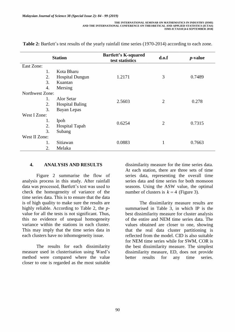
Table 2: Bartlett’s test results of the yearly rainfall time series (1970-2014) according to each zone.

Station Bartlett’s K-squared

test statistics d.o.f p-value

East Zone:

1.2171 3 0.7489

1. Kota Bharu

2. Hospital Dungun

3. Kuantan

4. Mersing

Northwest Zone:

2.5603 2 0.278 1. Alor Setar

2. Hospital Baling

3. Bayan Lepas

West I Zone:

0.6254 2 0.7315 1. Ipoh

2. Hospital Tapah

3. Subang

West II Zone:

0.0883 1 0.7663 1. Sitiawan

2. Melaka

4. ANALYSIS AND RESULTS

Figure 2 summarise the flow of

analysis process in this study. After rainfall

data was processed, Bartlett’s test was used to

check the homogeneity of variance of the

time series data. This is to ensure that the data

is of high quality to make sure the results are

highly reliable. According to Table 2, the p-

value for all the tests is not significant. Thus,

this no evidence of unequal homogeneity

variance within the stations in each cluster.

This may imply that the time series data in

each clusters have no inhomogeneity issue.

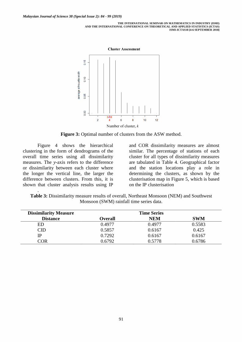
The results for each dissimilarity

measure used in clusterisation using Ward’s

method were compared where the value

closer to one is regarded as the most suitable

dissimilarity measure for the time series data.

At each station, there are three sets of time

series data, representing the overall time

series data and time series for both monsoon

seasons. Using the ASW value, the optimal

number of clusters is 4k (Figure 3).

The dissimilarity measure results are

summarised in Table 3, in which IP is the

best dissimilarity measure for cluster analysis

of the entire and NEM time series data. The

values obtained are closer to one, showing

that the real data cluster partitioning is

reflected from the model. CID is also suitable

for NEM time series while for SWM, COR is

the best dissimilarity measure. The simplest

dissimilarity measure, ED, does not provide

better results for any time series.





91

Figure 3: Optimal number of clusters from the ASW method.

Figure 4 shows the hierarchical

clustering in the form of dendrograms of the

overall time series using all dissimilarity

measures. The y-axis refers to the difference

or dissimilarity between each cluster where

the longer the vertical line, the larger the

difference between clusters. From this, it is

shown that cluster analysis results using IP

and COR dissimilarity measures are almost

similar. The percentage of stations of each

cluster for all types of dissimilarity measures

are tabulated in Table 4. Geographical factor

and the station locations play a role in

determining the clusters, as shown by the

clusterisation map in Figure 5, which is based

on the IP clusterisation

.

Table 3: Dissimilarity measure results of overall, Northeast Monsoon (NEM) and Southwest

Monsoon (SWM) rainfall time series data.

Dissimilarity Measure

Distance

Time Series

Overall NEM SWM

ED 0.4977 0.4977 0.5583

CID 0.5857 0.6167 0.425

IP 0.7292 0.6167 0.6167

COR 0.6792 0.5778 0.6786





92

Figure 4: Dendrograms of time series data in 12 stations with dissimilarity measures:

ED (A), CID (B), IP (C) and COR (D).

Table 4: The percentage number of stations for each cluster with different dissimilarity measures.

Cluster Dissimilarity Measures

ED CID IP COR

#1 66.70% 33.30% 41.70% 41.70%

#2 16.70% 33.30% 25.00% 25.00%

#3 8.30% 16.70% 25.00% 16.70%

#4 8.30% 16.70% 8.30% 16.70%





93

Figure 5: Clusterisation map of the Peninsular Malaysia rainfall data using IP dissimilarity measure

based on the overall data.

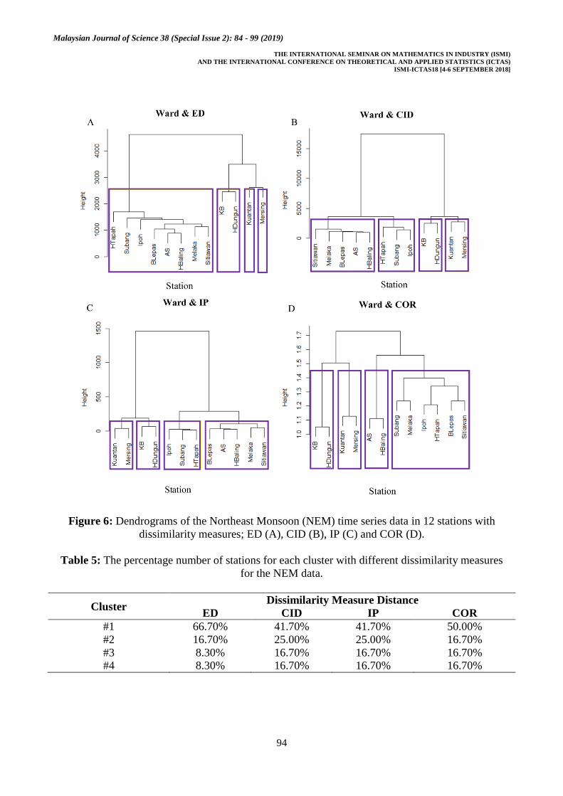
Figure 6 shows the cluster analysis

dendrograms of NEM time series data where

CID and IP distance measures produce

similar results. During NEM, the east coast

area of Peninsular Malaysia receives a lot of

rain, thus influencing the cluster analysis

results. The percentage number of stations of

each cluster for NEM time series data is

illustrated in Table 5 and the clusterisation

map is depicted in Figure 7.

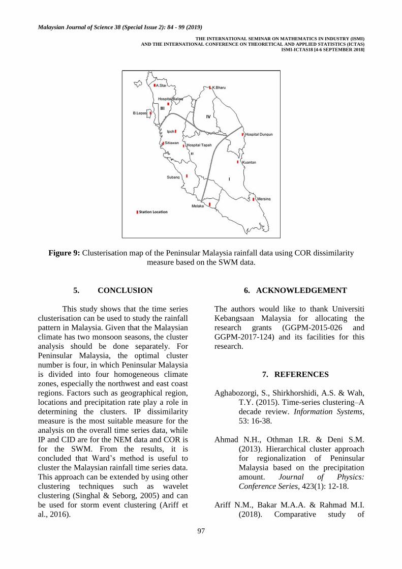
The cluster analysis dendrograms of SWM

time series data is shown in Figure 8, which

is different than the NEM time series data.

For SWM, the occurrence of rain is lower

than the NEM, this significantly influences

the determination of clusters than the NEM

time series data clusters. For the SWM time

series data, the percentage number of stations

of each cluster is illustrated in Table 6 and the

clusterisation map is depicted in Figure 9.





94

Figure 6: Dendrograms of the Northeast Monsoon (NEM) time series data in 12 stations with

dissimilarity measures; ED (A), CID (B), IP (C) and COR (D).

Table 5: The percentage number of stations for each cluster with different dissimilarity measures

for the NEM data.

Cluster Dissimilarity Measure Distance

ED CID IP COR

#1 66.70% 41.70% 41.70% 50.00%

#2 16.70% 25.00% 25.00% 16.70%

#3 8.30% 16.70% 16.70% 16.70%

#4 8.30% 16.70% 16.70% 16.70%





95

Figure 7: Clusterisation map of the Peninsular Malaysia rainfall data using CID or IP dissimilarity

measure based on the NEM data.





96

Figure 8: Dendrograms of the Southwest Monsoon (SWM) time series data in 12 stations with

dissimilarity measures; ED (A), CID (B), IP (C) and COR (D).

Table 6: The percentage number of stations of each cluster with different dissimilarity measures for

the SWM data.

Cluster Dissimilarity Measure Distances

ED CID IP COR

#1 50.00% 41.70% 33.30% 33.30%

#2 25.00% 25.00% 25.00% 33.30%

#3 16.70% 16.70% 25.00% 25.00%

#4 8.30% 16.70% 16.70% 8.30%





97

Figure 9: Clusterisation map of the Peninsular Malaysia rainfall data using COR dissimilarity

measure based on the SWM data.

5. CONCLUSION

This study shows that the time series

clusterisation can be used to study the rainfall

pattern in Malaysia. Given that the Malaysian

climate has two monsoon seasons, the cluster

analysis should be done separately. For

Peninsular Malaysia, the optimal cluster

number is four, in which Peninsular Malaysia

is divided into four homogeneous climate

zones, especially the northwest and east coast

regions. Factors such as geographical region,

locations and precipitation rate play a role in

determining the clusters. IP dissimilarity

measure is the most suitable measure for the

analysis on the overall time series data, while

IP and CID are for the NEM data and COR is

for the SWM. From the results, it is

concluded that Ward’s method is useful to

cluster the Malaysian rainfall time series data.

This approach can be extended by using other

clustering techniques such as wavelet

clustering (Singhal & Seborg, 2005) and can

be used for storm event clustering (Ariff et

al., 2016).

6. ACKNOWLEDGEMENT

The authors would like to thank Universiti

Kebangsaan Malaysia for allocating the

research grants (GGPM-2015-026 and

GGPM-2017-124) and its facilities for this

research.

7. REFERENCES

Aghabozorgi, S., Shirkhorshidi, A.S. & Wah,

T.Y. (2015). Time-series clustering–A

decade review. Information Systems,

53: 16-38.

Ahmad N.H., Othman I.R. & Deni S.M.

(2013). Hierarchical cluster approach

for regionalization of Peninsular

Malaysia based on the precipitation

amount. Journal of Physics:

Conference Series, 423(1): 12-18.

Ariff N.M., Bakar M.A.A. & Rahmad M.I.

(2018). Comparative study of





98

document clustering algorithms.

International Journal of Engineering

and Technology (UAE), 7(4): 246-

251.

Ariff N.M., Jemain A.A. & Bakar M.A.A.

(2016). Regionalization of IDF curves

with L-moments for storm events.

International Journal of Mathematical

and Computational Sciences, 10: 217-

223.

Arifin A.Z. & Asano A. (2006). Image

segmentation by histogram

thresholding using hierarchical cluster

analysis. Pattern Recognition Letters,

27(13): 1515-1521.

Batista G.E., Keogh E.J., Tataw O.M. & De

Souza V.M. (2014). CID: an efficient

complexity-invariant distance for time

series. Data Mining and Knowledge

Discovery, 28(3): 634-669.

Crétat J., Richard Y., Pohl B., Rouault M.,

Reason C. & Fauchereau N. (2012).

Recurrent daily rainfall patterns over

South Africa and associated dynamics

during the core of the austral summer.

International Journal of Climatology,

32(2): 261-273.

De Lucas D.C. (2010). Classification

Techniques for Time Series and

Functional Data. Universidad Carlos

III de Madrid. Doctoral dissertation.

DeGaetano A.T. (2001). Spatial grouping of

United States climate stations using a

hybrid clustering approach.

International Journal of Climatology,

21(7): 791-807.

Han J., Pei J. & Kamber M. (2012). Data

Mining: Concepts and Techniques 3rd

Edition. Waltham, M.A.: Morgan

Kaufmann Publishers.

Kavitha V. & Punithavalli M. (2010).

Clustering time series data stream–a

literature survey. International

Journal of Computer Science and

Information Security, 8(1):289-294.

Lin J. & Li Y. (2009). Finding Structural

Similarity in Time Series Data Using

Bag-of-Patterns Representation. In

Proceedings of the 21st International

Conference on Scientific and

Statistical Database Management,

461-477.

Michinaka T., Tachibana S. & Turner J.A.

(2011). Estimating price and income

elasticities of demand for forest

products: cluster analysis used as a

tool in grouping. Forest Policy and

Economics, 13(6): 435-445.

Munoz-Diaz D. & Rodrigo F.S. (2004).

Spatio-temporal patterns of seasonal

rainfall in Spain (1912-2000) using

cluster and principal component

analysis: comparison. Annales

Geophysicae, 22(5): 1435-1448.

Prasanna K.A.V.L. (2012). Performance

evaluation of multiviewpoint-based

similarity measure for data clustering.

Journal of Global Research in

Computer Science, 3(11): 21-26.

Ramos M.C. (2001). Divisive and

hierarchical clustering techniques to

analyse variability of rainfall

distribution patterns in a

Mediterranean region. Atmospheric

Research, 57(2):123-138.

Maharaj E.A., D’Urso P. & Galagedera D.U.

(2010). Wavelet-based fuzzy

clustering of time series. Journal of

Classification, 27(2): 231-275.





99

Rani, S. & Sikka, G. (2012). Recent

techniques of clustering of time series

data: a survey. International Journal

of Computer Applications, 52(15): 1-

9.

Soltani S. & Modarres R. (2006).

Classification of spatio-temporal

pattern of rainfall in Iran using a

hierarchical and divisive cluster

analysis. Journal of Spatial

Hydrology, 6(2): 1-12.

Tennant W.J. & Hewitson B.C. (2002). Intra-

seasonal rainfall characteristics and

their importance to the seasonal

prediction problem. International

Journal of Climatology: A Journal of

the Royal Meteorological Society,

22(9): 1033-1048.

Clustering of Rainfall Distribution Patterns in Peninsular ...

Documents

Transcript of Clustering of Rainfall Distribution Patterns in Peninsular ...