Climatic responses to anthropogenic groundwater exploitation…€¦ · · 2013-11-25Climatic...
21
Climatic responses to anthropogenic groundwater exploitation: a case study of the Haihe River Basin, Northern China Jing Zou • Zhenghui Xie • Yan Yu • Chesheng Zhan • Qin Sun Received: 15 December 2012 / Accepted: 4 November 2013 Ó Springer-Verlag Berlin Heidelberg 2013 Abstract In this study, a groundwater exploitation scheme is incorporated into the regional climate model, RegCM4, and the climatic responses to anthropogenic alteration of groundwater are then investigated over the Haihe River Basin in Northern China where groundwater resources are overexploited. The scheme models anthro- pogenic groundwater exploitation and water consumption, which are further divided into agricultural irrigation, industrial use and domestic use. Four 30-year on-line exploitation simulations and one control test without exploitation are conducted using the developed model with different water demands estimated from relevant socio- economic data. The results reveal that the groundwater exploitation and water consumption cause increasing wet- ting and cooling effects on the local land surface and in the lower troposphere, along with a rapidly declining groundwater table in the basin. The cooling and wetting effects also extended outside the basin, especially in the regions downwind of the prevailing westerly wind, where increased precipitation occurs. The changes in the four exploitation simulations positively relate to their different water demands and are highly non-linear. The largest changes in climatic variables usually appear in spring and summer, the time of crop growth. To gain further insights into the direct changes in land-surface variables due to groundwater exploitation regardless of the atmospheric feedbacks, three off-line simulations using the land surface model Community Land Model version 3.5 are also con- ducted to distinguish these direct changes on the land surface of the basin. The results indicate that the direct changes of land-surface variables respond linearly to water demand if the climatic feedbacks are not considered, while non-linear climatic feedbacks enhance the differences in the on-line exploitation simulations. Keywords Groundwater exploitation Climatic response Haihe River Basin Sensitivity test 1 Introduction Owing to population growth and economic development, human water demands are increasing rapidly and water is becoming scarce in many regions worldwide (Sha et al. 2003; Konikow and Kendy 2005). Due to its good water quality and easy exploitation, groundwater is widely used to meet human demands for water, especially in regions with sparse surface water supplies. However, excessive groundwater exploitation leads to declining terrestrial water storage, decreased stream flow, and weaker hydraulic connections between aquifers and rivers (Szilagyi 1999, J. Zou Z. Xie (&) Y. Yu Q. Sun State Key Laboratory of Numerical Modeling for Atmospheric Sciences and Geophysical Fluid Dynamics, Institute of Atmospheric Physics, Chinese Academy of Sciences, P.O. Box 9804, Beijing 100029, China e-mail: [email protected] URL: http://web.lasg.ac.cn/staff/xie/xie.htm J. Zou Y. Yu Q. Sun University of Chinese Academy of Sciences, Beijing 100049, China Present Address: J. Zou Institute of Oceanographic Instrumentation, Shandong Academy of Sciences, Qingdao 266001, China C. Zhan Key Laboratory of Water Cycle and Related Land Surface Process, Institute of Geographic Sciences and Natural Resources Research, Chinese Academy of Sciences, Beijing 100101, China 123 Clim Dyn DOI 10.1007/s00382-013-1995-2
Transcript of Climatic responses to anthropogenic groundwater exploitation…€¦ · · 2013-11-25Climatic...

Climatic responses to anthropogenic groundwater exploitation:a case study of the Haihe River Basin, Northern China
Jing Zou • Zhenghui Xie • Yan Yu •
Chesheng Zhan • Qin Sun
Received: 15 December 2012 / Accepted: 4 November 2013
� Springer-Verlag Berlin Heidelberg 2013
Abstract In this study, a groundwater exploitation
scheme is incorporated into the regional climate model,
RegCM4, and the climatic responses to anthropogenic
alteration of groundwater are then investigated over the
Haihe River Basin in Northern China where groundwater
resources are overexploited. The scheme models anthro-
pogenic groundwater exploitation and water consumption,
which are further divided into agricultural irrigation,
industrial use and domestic use. Four 30-year on-line
exploitation simulations and one control test without
exploitation are conducted using the developed model with
different water demands estimated from relevant socio-
economic data. The results reveal that the groundwater
exploitation and water consumption cause increasing wet-
ting and cooling effects on the local land surface and in the
lower troposphere, along with a rapidly declining
groundwater table in the basin. The cooling and wetting
effects also extended outside the basin, especially in the
regions downwind of the prevailing westerly wind, where
increased precipitation occurs. The changes in the four
exploitation simulations positively relate to their different
water demands and are highly non-linear. The largest
changes in climatic variables usually appear in spring and
summer, the time of crop growth. To gain further insights
into the direct changes in land-surface variables due to
groundwater exploitation regardless of the atmospheric
feedbacks, three off-line simulations using the land surface
model Community Land Model version 3.5 are also con-
ducted to distinguish these direct changes on the land
surface of the basin. The results indicate that the direct
changes of land-surface variables respond linearly to water
demand if the climatic feedbacks are not considered, while
non-linear climatic feedbacks enhance the differences in
the on-line exploitation simulations.
Keywords Groundwater exploitation � Climatic
response � Haihe River Basin � Sensitivity test
1 Introduction
Owing to population growth and economic development,
human water demands are increasing rapidly and water is
becoming scarce in many regions worldwide (Sha et al.
2003; Konikow and Kendy 2005). Due to its good water
quality and easy exploitation, groundwater is widely used
to meet human demands for water, especially in regions
with sparse surface water supplies. However, excessive
groundwater exploitation leads to declining terrestrial
water storage, decreased stream flow, and weaker hydraulic
connections between aquifers and rivers (Szilagyi 1999,
J. Zou � Z. Xie (&) � Y. Yu � Q. Sun
State Key Laboratory of Numerical Modeling for Atmospheric
Sciences and Geophysical Fluid Dynamics, Institute of
Atmospheric Physics, Chinese Academy of Sciences,
P.O. Box 9804, Beijing 100029, China
e-mail: [email protected]
URL: http://web.lasg.ac.cn/staff/xie/xie.htm
J. Zou � Y. Yu � Q. Sun
University of Chinese Academy of Sciences,
Beijing 100049, China
Present Address:
J. Zou
Institute of Oceanographic Instrumentation, Shandong Academy
of Sciences, Qingdao 266001, China
C. Zhan
Key Laboratory of Water Cycle and Related Land Surface
Process, Institute of Geographic Sciences and Natural Resources
Research, Chinese Academy of Sciences, Beijing 100101, China
123
Clim Dyn
DOI 10.1007/s00382-013-1995-2

2001; Kollet and Zlotnik 2003; Biggs et al. 2008). Water
consumption processes have also been shown to enhance
evapotranspiration and reduce local temperature (Douglas
et al. 2009; Sacks et al. 2009). Moreover, increasing water
vapor from land may lead to more local convection and
further changes in atmospheric motions (Kueppers et al.
2007; Saeed et al. 2009; DeAngelis et al. 2010; Harding
and Snyder 2012; Qian et al. 2013). Therefore, continually
pumping groundwater each year for consumption causes
not only a local decline in the groundwater table, but also
alters the water cycle and energy budget, which ultimately
affects the regional climate (Moore and Rojstaczer 2002;
Chen and Hu 2004; Yuan et al. 2008; Kustu et al. 2010).
Numerous modeling studies have demonstrated the effects
of groundwater exploitation and use on land-surface hydro-
logical processes. Some researchers used water resource
models or hydrological models to simulate the process of
water resource withdrawal and use. Hanasaki et al. (2008)
developed an integrated water resource model, which con-
sidered anthropogenic reservoir operation, water withdrawal,
and agricultural irrigation. Doll et al. (2012) used the global
water resources and use model (WaterGAP) to analyze the
impact of groundwater exploitation on global land water
storage and found that it had negative effects on local water
storage in areas dominated by groundwater irrigation.
These water resource models or hydrological models
usually include detailed descriptions of groundwater
exploitation and use, but their deficiencies in terms of
energy, biophysics and other processes make it difficult to
detect the effects of groundwater exploitation and use on
the land-surface energy or other processes. Besides the
implementation of water resource models, many studies
have used land surface models to investigate the effects of
water withdrawal and use on land surface processes.
Haddeland et al. (2006) incorporated an irrigation scheme
into the Variable Infiltration Capacity model and found that
agricultural irrigation led to increased evapotranspiration
and decreased air temperature in the Colorado and Mekong
river basins in simulations using the scheme. Ozdogan
et al. (2010) incorporated irrigation and crop-type infor-
mation from satellite remote sensing into the land surface
model LSM, and found that the irrigation caused a 12 %
increase in evapotranspiration and an equivalent reduction
in sensible heat flux in the growing seasons. Pokhrel et al.
(2012) incorporated water regulation modules and an irri-
gation scheme into the Minimal Advanced Treatments of
Surface Interaction and Runoff (MATSIRO) model and
found a maximum increase of about 50 W/m2 in latent heat
flux from June to August due to irrigation.
However, most of these modeling studies of the
hydrological or land-surface effects of groundwater
exploitation did not consider the feedbacks between cli-
mate and groundwater consumption. Although many
studies have used climate models to investigate such
feedbacks, they usually focused on the climatic responses
due to irrigation, since this process constitutes a major
proportion of water consumption (Shiklomanov 2000; Ri-
jsberman 2006). Puma and Cook (2010) investigated global
irrigation effects during the twentieth century using the
Goddard Institute for Space Studies (GISS) ModelE, and
found a significant reduction in temperature and increase in
precipitation in the Northern Hemisphere since the 1950s.
Chen and Xie (2010) investigated the irrigation effects of
an inter-basin water transfer project using the regional
climate model RegCM3 and found more local evapo-
transpiration via an increase of soil moisture and more
precipitation because of changes in the surface water and
energy balances.
Generally, the studies using climate models to assess the
climatic responses to irrigation have not considered local
groundwater exploitation or other types of water con-
sumption (Adegoke et al. 2003; Boucher et al. 2004; Lobell
et al. 2008; Sacks et al. 2009; Kueppers and Snyder 2012).
Instead, they treated irrigation water as being pumped from
land-surface water bodies, such as nearby lakes or reser-
voirs, which are not considered in the water cycle frame-
work of the climate models. This approach of including
irrigation water is not suitable for regions dominated by
groundwater irrigation and makes it difficult to specify the
limits on the quantity of water supplied by surface water
bodies. Besides, other methods of water consumption, such
as domestic and industrial use, should be considered, and
the climatic responses of water exploitation and con-
sumption should also be considered integrally as a whole
within the water cycle framework of models because water
resource exploitation and consumption interact with each
other and no elements can be neglected. In order to
investigate the total climatic responses to groundwater
exploitation and consumption, this study incorporates a
simple scheme into a regional climate model. The Haihe
River Basin, where groundwater is severely over-exploited,
is selected as the study domain.
In Sect. 2 of this paper, the regional climate model used
and the scheme developed are described, while Sect. 3
introduces the study domain, estimation of water demand
and setup of simulation tests, the results of the simulation
are provided in Sect. 4 and the conclusions and discussion
are presented in Sect. 5.
2 Model development
2.1 The regional climate model RegCM4
RegCM4 is a regional climate model developed by the
International Center for Theoretical Physics in Italy (Giorgi
J. Zou et al.
123

and Anyah 2012; Giorgi et al. 2012). The dynamic core of
RegCM4 originates from the hydrostatic version of the
fifth-generation Pennsylvania State University/National
Center for Atmospheric Research mesoscale model (Grell
et al. 1994). Three convective precipitation schemes (Kuo,
Grell, Emanuel) and one large-scale precipitation scheme
(SUBEX) are available for its precipitation simulation
(Giorgi et al. 1993). Its land surface module is optional,
with BATS1e (Dickinson et al. 1993) and the Community
Land Model version 3.5 (CLM3.5) (Oleson et al. 2004,
2008) available for employment. In this study, CLM3.5 is
used.
The land surface model CLM3.5 was developed by the
National Center of Atmospheric Research, USA. The
model uses a tile approach to describe the heterogeneity of
the land surface. Each grid cell contains four land cover
types (glacier, wetland, lake, vegetation), and the vegetated
fraction can be further divided into 17 different plant
function types. The model also contains five possible snow
layers and ten soil layers with an unconfined aquifer below
in the vertical direction. The RegCM4 and CLM3.5 per-
form well for simulation of spatial and temporal climatic
features worldwide, which can be used for further sensi-
tivity tests (Tian et al. 2008; Wang and Zeng 2011; Gao
et al. 2012; Ozturk et al. 2012). In CLM3.5, the parame-
terization of the runoff process is based on the SIMTOP
model developed by Niu et al. (2005, 2007). The ground-
water table can be within or below the soil layers,
depending on the changes of water storage. The aquifer
water storage Wa (mm) is calculated by:
dq �Wa
dt¼ qrecharge � qdrai; ð1Þ
where q is density of water and equal to 1.0 9 103 kg/m3;
t is the time step (s); qrecharge is recharge from soil layers to
aquifers (kg m-2 s-1) and qdrai is groundwater outflow
(kg m-2 s-1).
The groundwater recharge qrecharge (kg m-2 s-1) is
expressed as:
qrecharge ¼ �ka
�103zr � w10 � 103z10ð Þ103 zr � z10ð Þ ; ð2Þ
where ka is the hydraulic conductivity of the aquifer
(kg m-2 s-1); z5 is the depth of the groundwater table (m);
w10 is the matric potential of the 10th soil layer (m); and z10
is the depth to the midpoint of the 10th soil layer (node
depth) (m).
The calculation of soil temperature is based on the
energy balance on land surface. The heat flux into the
snow/soil surface from the atmosphere (h) (W m-2) is
defined as:
h ¼ Sg � Lg � Hg � kEg; ð3Þ
where Sg is the solar radiation absorbed by the ground
(W m-2); Lg is the longwave radiation emitted by the
ground (W m-2); Hg is the sensible heat flux from the
ground (W m-2); and kEg is the latent heat flux from the
ground (W m-2). The heat flux from the soil bottom is set
as zero.
2.2 A groundwater exploitation scheme and its
implementation in RegCM4
We present a scheme describing the anthropogenic
groundwater exploitation and consumption in the regional
climate model RegCM4. As shown in Fig. 1, the stream
flow and groundwater resource in each grid cell are
exploited to meet the given human water demand Dt in unit
time and area (kg m-2 s-1). The fluxes of exploited river
water and groundwater are termed Qs (kg m-2 s-1) and Qg
(kg m-2 s-1), respectively.
The consumption of total exploited water resources is
divided into three parts: agricultural irrigation Da
(kg m-2 s-1), industrial consumption Di (kg m-2 s-1) and
domestic consumption Dd (kg m-2 s-1). The water con-
sumed by irrigation is treated as effective rainfall reaching
the topsoil; the industrial and domestic water consumptions
are treated as being consumed through evaporation and
wastewater discharge into stream channels (Wr)
(kg m-2 s-1).
Fig. 1 Framework of simulated human-induced water resource
exploitation and consumption process. The water is pumped from
rivers and underground aquifers to meet the demand, and the demand
is divided into industrial, domestic and irrigation water. The water
consumed by industrial and domestic sections partly increases local
evaporation and partly return into water channels. The water
consumed by irrigation is treated as effective rainfall reaching the
soil surface
Climatic responses to anthropogenic groundwater exploitation
123

The scheme is then incorporated into CLM3.5, the land
surface module of RegCM4. Water flux exploited from
rivers, Qs, is subtracted from the water quantity in rivers.
The flux of groundwater exploitation Qg is introduced into
the calculation of water storage in CLM3.5, and is removed
from the water storage in each time step, which can be
expressed as follows:
qWa;nþ1 � qWa;n ¼ qrecharge � qdrain � Qg
� �Dt; ð4Þ
where Wa,n?1 and Wa,n are the aquifer water storage Wa
(mm) in time steps n ? 1 and n, respectively; and Dt is
time step (s) in the simulations.
In the land surface water consumption process, the
effective rainfall in the model increases by Da due to
irrigation. The wastewater recharge into rivers from the
industrial and domestic consumption (Wr) is defined as
a(Di ? Dd) and is treated as being removed from the
column of grid cells and never reused. The remaining
water is used to increase the evaporation by (1 - a) 9
(Di ? Dd).
As seen in Fig. 2, based on the proposed scheme, other
land-surface variables will subsequently change due to
perturbations of water storage, evaporation and effective
rainfall on the land surface: these can be considered as the
direct effects of groundwater exploitation and consump-
tion. Changes in the atmosphere induced by interactions
between the land surface and atmosphere will further affect
the land surface via changes in air temperature, humidity,
precipitation, etc., and these can be considered as indirect
effects.
3 Study domain and experimental design
3.1 The study domain
The Haihe River Basin, which lies in northern China,
covers an area of 318,200 km2. Mountains and plateaus in
the west and north of the basin account for 60 % of the
total area, while plains with a lower altitude in the east and
south, where most inhabitants live, account for the
remaining 40 %. Figure 3a shows the fractions of different
crop types in the grid cells used in RegCM4/CLM3.5, and
most crops are planted in the plain areas of the basin. The
Haihe River Basin is a semi-humid monsoon region with
an annual precipitation of 500–700 mm (Ren et al. 2002;
Yang and Tian 2009; Liang et al. 2011). Due to its rapidly
growing economy, the basin is facing an increasingly
serious imbalance between low precipitation and high
water demand. Relevant studies have shown that 40 % of
rivers in the basin have now turned into seasonal rivers and
90 % of wetlands have now disappeared when compared
with the status in the 1950s, owing to the rapid ground-
water exploitation in the region (Xia and Zhang 2008).
Exhausting groundwater resources, ecological degradation
and stream flow depletion are threatening the sustainable
development of this political center of China (Xia and
Chen 2001; Xu et al. 2004; Jia et al. 2012).
3.2 Estimating the water supply and demand
in the proposed scheme
Based on the framework of the proposed scheme and on
real conditions and parameters in the study domain, the
water supply and demand in the scheme are estimated. In
this study, some assumptions are made, as follows. Firstly,
the local natural water resource is set to be able to meet the
human water demand, which can be expressed as the bal-
ance of water supply and demand:
Qg þ Qs ¼ Dt: ð5Þ
Once the local water resource is exhausted at some time
step, the water exploitation and consumption process will
totally cease until a balance of supply and demand is
achieved. Secondly, because of the limits of the structure in
RegCM4, we do not consider the routing of water through
the river system. Therefore, the stream flow in river
channels for exploitation is assumed to be the local total
runoff, equal to the sum of surface runoff Rsur
(kg m-2 s-1) and subsurface runoff Rsub (kg m-2 s-1)
generated in each grid cell. Thirdly, the groundwater
resource exploitation is set to occur only if the total runoff
generated in each grid cannot meet the water demand in
each time step, which can be expressed as:Fig. 2 Sketch of interactions between the atmosphere and land
surface in RegCM4
J. Zou et al.
123

Qg ¼ max 0; Dt � Rsur � Rsubð Þ½ �: ð6Þ
The annual volume of water demand in each grid cell is
estimated according to relevant socioeconomic data of the
Haihe River Basin collected in A.D. 2000 and is taken to
remain constant in this study. This volume is noted as
M2000 (m3 year-1), and calculated by:
M2000 ¼ kq�1DtS ¼ c1Apop þ bc2AGDP þ c3Aagr; ð7Þ
where k is constant and equal to 31,536,000 s year-1; q is
equal to 1.0 9 103 kg m-3; Dt is water demand
(kg m-2 s-1); S is the area of grid cell (m2); c1 is the
averaged annual domestic water consumption per capita,
here equal to 40.64 m3 capita-1 year-1; Apop is the popu-
lation in the grid cell (capita); b is an empirical conversion
ratio between GDP and the value of industrial output, equal
to 1.42; c2 is the averaged annual industrial water con-
sumption per yuan of industrial output, here equal to
40.65 9 10-4 m3 yuan-1 year-1; AGDP is the gross
domestic product (GDP) in the grid cell (yuan); c3 is the
averaged annual agricultural water consumption per unit
area of cropland, here equal to 0.414 m3 hectare-1 year-1;
Aagr is the area of agricultural land in the grid cell (hect-
are). The socioeconomic data in Haihe River Basin were
obtained from the Data Center for Resources and Envi-
ronment of Sciences, Chinese Academy of Sciences (http://
www.resdc.cn/english/default.asp). This socioeconomic
dataset has a spatial distribution of 1 km 9 1 km and is
then averaged onto grids of 30 km 9 30 km, in order to
match the grids used in the RegCM4 model.
The accumulated volume of estimated water demand
over the basin in 2000,P
i Mi;2000 (i is the index of grid
cell), is shown in Table 1. The statistical data for com-
parison are from China Water Resource Bulletin and are
available in Chinese at http://www.chinawater.net.cn/
WaterRes/2000/. A higher water demand is estimated as
shown in Table 1, probably because of the constant rate of
water consumption, the empirical ratio and different sour-
ces of data. In the rural regions of the basin, the level of
agricultural irrigation by pumping water from wells is
usually hard to determine, and the statistical data from
different agencies has great uncertainties. Therefore, the
greatest difference appears in the estimated agricultural
(a) (b)
(d)(c)
Fig. 3 Spatial distribution of a the crop fraction of the grid cell in the study domain; b estimated water demand for the basin; c topography of the
study domain; d groundwater depth after spin-up
Table 1 Total estimated water
demand and actual statistical
water consumption in 2000 over
the basin
Industrial use
(108 m3 year-1)
Domestic use
(108 m3 year-1)
Agricultural use
(108 m3 year-1)
Total quantity
(108 m3 year-1)
Actual 65.7 51.8 280.9 398.4
Estimated 80.6 50.8 357.2 488.6
Climatic responses to anthropogenic groundwater exploitation
123

demand. The spatial distribution of volume of estimated
water demand, M2000, is shown in Fig. 3b. More water is
needed in the southern and eastern plains of the basin than
in the northern and western mountainous regions. Cities in
the plains of the basin such as Shijiazhuang (114.5�E,
38�N), Tianjin (117�E, 39�N), Beijing (116.5�E, 40�N) and
their surrounding areas have the largest water demands due
to their dense population and industrial establishments.
The proportion of wastewater discharged into streams,
a, is arbitrarily set as 30 % of the water for industrial and
domestic consumption based on a small scale survey (Mao
et al. 2000). In fact, the wastewater returned to streams
does not flow into the sea entirely and may be re-treated for
landscaping and other municipal facilities, especially in
regions with scarce water resources. According to Shiklo-
manov (2000), about 85–90 % of industrial and domestic
water is returned to the streams. This proportion is a pri-
mary utilization ratio and does not include the other
methods of consumption before the waste water flows into
the sea. However, in the simple scheme proposed in this
paper, the water resources cannot be reused; therefore, we
greatly simplify this dissipation process and regard most of
the industrial and domestic water use as being consumed
by evaporation. The 70 % of industrial and domestic water
lost by evaporation not only includes water consumption in
the factories or residential communities, but also includes
the dissipation process of waste water flowing from the
factories or residential communities, which is distinct from
the primary proportion of municipal water use. According
to the Water Resource Bulletin of Haihe River Basin
in 2000 (http://www.hwcc.gov.cn/pub/hwcc/static/szygb/
gongbao_2000/), the volume of river discharge into the
sea was only 4.1 9 108 m3 in 2000, far less than the water
demands in the basin. The low discharge into the sea
indicates that the wastewater from factories and residential
communities is still consumed in the basin.
3.3 Experimental design
As shown in Table 2, five on-line simulation tests using
RegCM4 from 1971 to 2000 were conducted to explore
changes in regional climate caused by human-induced
groundwater exploitation and consumption. The control
test (CTL) simulates the natural state, ignoring human-
induced perturbations; the exploitation test 1 (Test 1) uses
the fixed total water demand, Dt (kg m-2 s-1), estimated in
2000; exploitation test 2 (Test 2) uses half of the demand
used in Test 1 and the same water allocation proportions;
exploitation test 3 (Test 3) uses estimated linearly
increasing annual water demands, D (kg m-2 s-1), with
the Dt estimated in 2000. The total volume of water
demand over the basin in the year y, which is noted asPi Mi;y, can be estimated by
X
i
Mi;y ¼X
i
kq�1Di;ySi ¼ ð5:74� y� 10991:4Þ � 108;
ð8Þ
where k is 31,536,000 s year-1; q is 1.0 9 103 kg m-3;
Di,y is the water demand (kg m-2 s-1) of the grid i in the
year y; Si is the area of grid i (m2); y is the year. In 2000,
the demand D in Test 3 is equal to Dt. Data for the linear
fitting of historic water demand were derived from the
Water Resource Bulletin of Haihe River Basin and Water
Resource Assessment in Haihe River Basin (Ren 2007)
written in Chinese. Although the historic water demand is
not available every year, the estimated linear equation fits
the data well. Exploitation test 4 (Test 4) uses the fixed
total water demand in 2000 as used in Test 1, but it con-
siders the temporal allocation of irrigation water within a
year, in contrast to the other three on-line exploitation tests,
which have no seasonal variations of irrigation water. The
domestic and industrial water consumption sections have
no seasonal variations, which is same as Test 1. In Test 4,
the irrigation date is set in advance according to the
planting dates of winter wheat and summer maize, the chief
crops in Haihe River Basin. The spring irrigation starts on
March 10, when the winter wheat turns green after the
dormancy in winter, and stops on June 18, when the winter
wheat is harvested. The summer irrigation starts on June
22, the planting time of summer maize, and stops on
August 28, the harvest time of summer maize. The date for
winter wheat turning green is the simple mean value of the
dataset for crop growth and development from 1992 to
2010 in the China Meteorological Data Sharing System
(http://cdc.cma.gov.cn). The dates of harvest for winter
Table 2 Description of constructed simulation tests
Model
used
Annual water demand Irrigation date
CTL RegCM4/
CLM3.5
None None
Test 1 Same as
CTL
Fixed, Dt in 2000 All the year
round
Test 2 Same as
CTL
Fixed, half of Dt in 2000 Same as Test 1
Test 3 Same as
CTL
Variable, linearly
increasing demand
from 1971 to 2000
Same as Test 1
Test 4 Same as
CTL
Same as Test 1 March 10–June
18, June 22–
August 28
CTL_off CLM3.5 None None
Test
1_off
Same as
CTL_off
Same as Test 1 Same as Test 1
Test
2_off
Same as
CTL_off
Same as Test 2 Same as Test 1
J. Zou et al.
123

wheat, planting and harvest for summer maize are derived
from China Agricultural Phenology Atlas by Zhang et al.
(1987). The irrigation water in the four exploitation tests
has no diurnal variations and is equally allocated
throughout the day. Based on the designed simulation tests,
the climatic responses to different water demands can be
detected by comparing Tests 1, 2 and 3; the effects of
seasonal irrigation can also be investigated by comparing
Tests 1 and 4.
Additionally, to identify the roles of both direct changes
and indirect climatic feedbacks of groundwater exploita-
tion and consumption in the basin, three off-line tests from
1971 to 2000 were conducted by CLM3.5 with the same
water demands as those in the on-line tests CTL, Test 1 and
Test 2. They are named as CTL_off, Test 1_off and Test
2_off, respectively.
The RegCM4 model is centered at 116�E, 38�N, with a
resolution of 30 km 9 30 km. ERA40 reanalysis data are
used as the lateral boundary forcing for the model. The
CLM option and Grell scheme are selected as the model’s
land surface scheme and convective precipitation scheme
respectively. The time step is 100 s for the atmosphere
module and 30 min for the land surface module. The
altitude of the simulated region is shown in Fig. 3c and
the area of the Haihe River Basin is enclosed by the black
line.
Before the on-line simulations, an off-line spin-up of
500 years using CLM3.5 is performed before the sim-
ulation tests started, repeatedly driven by the prepared
atmospheric output of RegCM4 from 1961 to 1970 for
50 times. Based on the final result of the off-line spin-
up, a 10-year on-line spin-up without exploitation pro-
cesses using RegCM4 is continued from 1961 to 1970,
in order to provide a balanced climatology and elimi-
nate the disparity of balanced status between off-line
and on-line tests. For the three off-line tests, a simula-
tion from 1961 to 1970 using CLM3.5 without the
exploitation scheme is performed, based on the final
status of the off-line spin-up of 100 years. The three
off-line simulation tests use the final state in 1970 as
initial conditions and start from 1971 with different
water demands. The off-line simulations are all driven
by the output of the on-line CTL test by RegCM4 from
1961 to 2000, and their time step is also 30 min. The
land surface data used in the off-line simulations are the
same as those in the on-line cases.
The groundwater depths after spin-up, which are
shown in Fig. 3d, correlate well with the regional cli-
matology. Specifically, the north-western desert and
grassland regions in the figures have deeper groundwater,
while in the humid regions in the south-east the soil has
higher moisture content and the water table is closer to
the land surface.
4 Results
4.1 Validation of the control test (CTL)
Observed precipitation and 2 m air temperature data from
1971 to 2000, interpolated from meteorology stations in
China, are used for validation of the control test (CTL)
(Xie et al. 2007). The groundwater table data for the Haihe
River Basin in 2000 are derived from the Ministry of Water
Resource and Institute for Geo-Environmental Monitoring
in China. Because of the sparse observations, the observed
values of groundwater table in the grid cells without
observations are set as missing values. Figure 4a–d show
the spatial distributions of the 30-year mean precipitation
and 2 m air temperature. The control test run by RegCM4
performs well for simulation of the regional climatology.
Specifically, the mean simulated precipitation and tem-
perature decrease from south to north, which is consistent
with the observations. However, in the Haihe River Basin,
a higher temperature of about 1 K in the control test reveals
a certain bias that needed improvement when compared to
the observed data. The simulated precipitation in the basin
is slightly higher on average by about 100 mm/year, except
for the southern plains of the basin, where less precipitation
is modeled.
In addition to spatial distribution, the temporal correla-
tion coefficient (CC), standard deviation (STD) and root-
mean-square error (RMSE) are employed to quantify the
model’s performance. The averaged statistics for the Haihe
River Basin given in Table 3 indicate that RegCM4 is able
to simulate the temporal variability of regional climate in
the basin well.
Meanwhile, because of the poorly characterized human
activities, shallower groundwater is simulated by the CTL
test in the Haihe River Basin, where the land water
resources are greatly impacted by human beings. Here,
the mean groundwater table in 2000 simulated by Test 1
is presented instead of the CTL test, for comparison with
the observations. Figure 4e shows the observed ground-
water table averaged from 173 observation wells in 2000.
As shown in Fig. 4f, the groundwater table simulated by
Test 1 in the plain region of the basin is broadly equiv-
alent to the observations in magnitude. However, there is
still a large bias between the simulation and observations.
The changes in groundwater table simulated by Test 1 do
not correspond exactly with the observations. In some
areas near Shijiazhuang (114.5�E, 38�N) and Tianjin
(117�E, 39�N), the observed groundwater table is still
deeper than that in Test 1. This may be because the model
cannot consider the lateral flow of groundwater, and
regards the aquifers as being homogeneous. The scheme
of local exploitation cannot consider the groundwater
lateral flow and the transfer of exploited water resource
Climatic responses to anthropogenic groundwater exploitation
123

between grid cells in regions of high water demand.
Besides, the estimated water demand in 2000 is relatively
higher than the statistical average. Less available surface
water in the simulations due to the use of local runoff
instead of streamflow also leads to larger groundwater
pumping, especially in the downstream regions with large
streamflow. The Fig. 4g shows the yearly groundwater
table levels obtained by the CTL test, Test 1, and the
observations. The observed data are also averaged from
the 173 wells in the basin and are only available from
1991 to 2000. As seen in the figure, the groundwater
predicted by the CTL test is shallower than the observed
data, while the groundwater table predicted by Test 1 is
deeper because of the high water demand. Although the
simulations present decreasing trends of groundwater, the
rise of the observed groundwater table from 1992 to 1997
(a) (b)
(d)(c)
(e)
(g)
(f)
Fig. 4 Spatial distribution of a mean precipitation observed; b mean
precipitation simulated by CTL; c mean 2 m air temperature
observed; d mean 2 m air temperature simulated by CTL; e mean
groundwater table observed in 2000; f mean groundwater table
simulated by Test 1 in 2000; g the basin-averaged time series of
groundwater table by CTL, Test 1 and observation
J. Zou et al.
123

cannot be simulated by the CTL and Test 1. Additionally,
the declining trends of water table depth in the simula-
tions are mainly attributed to the declining trend of sim-
ulated precipitation, not the reason of spin-up when
compared with the basin-averaged time series of precip-
itation by CTL (not shown).
4.2 Effects of anthropogenic groundwater exploitation
on regional climate
4.2.1 Spatial distribution and differences in the vertical
profiles
The 30-year groundwater exploitation and use have chan-
ged the climate in the local basin and its surrounding
regions. The multi-year mean spatial distributions of dif-
ferences between Test 1, Test 2, Test 3 and CTL are pre-
sented as follows. As shown in Fig. 5a–c, a significantly
dropping groundwater table appears across the southern
plains of the basin due to long-term exploitation. However,
the mountainous regions in the west and north of the basin
did not suffer significant groundwater depletion because of
their sparse population and low water demand. The areas
shaded by strips in Figs. 5, 6, 7 and 8 are at or exceed the
95 % confidence level, based on the t test. The differences
in groundwater shown in Fig. 5a–c are positively corre-
lated with their respective water demands, and the differ-
ence between Test 2 and CTL approaches half of the
difference between Test 1 and CTL. The difference
between Test 3 and CTL (Fig. 5c) is between Fig. 5a, b in
magnitude.
The differences in other climatic variables do not
change linearly like the groundwater table because of the
highly nonlinear responses of the climate system. Differ-
ences in total soil moisture are shown in Fig. 5d–f. In the
three exploitation tests, a great proportion of their water
demand is consumed by agricultural irrigation, which is
treated as effective rainfall. Additionally, in CLM3.5, there
are different root fractions in the soil layers, and the tran-
spiration in each layer depends on the soil water and root
fraction in each soil layer. The recharge from soil layers
into the aquifers depends on the depth of the groundwater
table, and when the groundwater depth approaches infinity,
the recharge will approach its maximum infiltration
capacity. In this way, more water infiltrates into the upper
soil layers and increases the soil moisture there, but the
altered transpiration in each soil layer and increased
recharge into aquifers below also affects the moisture in
lower soil layers. The changes in total soil moisture depend
on these combined effects. As shown in Fig. 5d, signifi-
cantly increased total soil moisture is detected in the basin
because of heavy irrigation in Test 1. The soil moisture
outside of the basin to the northeast and south also increase
due to changes in precipitation. For Test 2 in Fig. 5e, the
reduced irrigation does not cause an increase in total soil
moisture. Rather, drier soil is detected in the north and
south of plain regions of the basin. In the regions outside
the basin, no significant changes in total soil moisture are
detected. Slightly wetter soil to the south and drier soil to
the northeast of the basin corresponded well with the
spatial distribution of the precipitation difference shown in
Fig. 6e. In Test 3, the soil moisture increases in most parts
of the basin, especially in the northwest regions.
The differences in total runoff generated shown in
Fig. 5g–i are affected by both soil moisture and the
groundwater table. In the three exploitation tests, a wetter
top soil layer due to irrigation causes more surface runoff
to be generated in the basin, while reducing the ground-
water table and changes in moisture in the lower soil layers
also constrain the generation of subsurface runoff. There-
fore, the changes in total runoff are affected by the wetter
upper soil layers due to irrigation and the lowered
groundwater table. As shown in Fig. 5g, for Test 1, greater
differences are detected in the northern and western
mountainous regions where the groundwater does not
suffer rapid depletion, while no apparent differences are
observed in the southern regions of the basin because of the
combined effects of a dropping groundwater table and
increased soil moisture. More runoff is also detected to the
south and northeast of the basin due to increased soil
moisture in that region. As shown in Fig. 5h, for Test 2, the
spatial distribution of differences is much less than half of
the differences between Test 1 and CTL, which corre-
sponds well with the distribution of total soil moisture. For
Test 3 shown in Fig. 5i, the spatial distribution of runoff
differences is similar to that for Test 1 in Fig. 5g, except
for its smaller magnitude.
Figure 5j–l show the differences in evapotranspiration
in Tests 1, 2 and 3. In the Haihe River Basin, most resi-
dents, farmland and industrial facilities are in the plain
areas, where the evapotranspiration increases most in the
Table 3 Statistics of control test in the Haihe River Basin
CC RMSE STD
Observed Modeled
Precipitation 0.77 1.31 mm/day 1.83 mm/day 1.78 mm/day
Temperature 0.89 5.22 K 10.83 K 10.16 K
Correlation Coefficient: CC ¼Pn
i¼1xmi�xmð Þ xoi�xoð ÞffiffiffiffiffiffiffiffiffiffiffiffiffiffiffiffiffiffiffiffiffiffiffiffiffiffiffiffiffiffiffiffiffiffiffiffiffiffiffiffiffiffiffiffiffiffiffiffiPn
i¼1xmi�xmð Þ2 �
Pn
i¼1xoi�xoð Þ2
p ; xmi and xoi
are the simulated and observed mean monthly precipitation/tem-
perature in months i, respectively, n is the number of months; Root
Mean Square Error: RMSE ¼ffiffiffiffiffiffiffiffiffiffiffiffiffiffiffiffiffiffiffiffiffiffiffiffiffiffiffiffiffiffiffiffiffiffiffiffiffi1n
Pni¼1 xmi � xoið Þ2
q; Standard Devi-
ation: STD ¼ffiffiffiffiffiffiffiffiffiffiffiffiffiffiffiffiffiffiffiffiffiffiffiffiffiffiffiffiffiffiffi1n
Pni¼1 xi � xð Þ2
q
Climatic responses to anthropogenic groundwater exploitation
123

basin. Statistically significant increases are detected in the
plain areas for Test 1 in Fig. 5j, but not for Tests 2 and 3 in
Fig. 5k, l. The largest increase in evapotranspiration is in
areas near Shijiazhuang (114.5�E, 38�N), corresponding
with the pattern of water demands and changes in the
groundwater table.
As more water is pumped from underground and
increases local evaporation, more moisture is transferred to
the lower troposphere, which enhances local convective
activities and causes changes in regional atmospheric cir-
culation. More atmospheric humidity is detected in the
exploitation tests, which leads to increased probabilities of
precipitation events. As shown in Fig. 6a, for Test 1, a
wetter atmosphere at 850 hPa appears in the eastern por-
tion of the basin, where more precipitation is detected. The
atmosphere also becomes wetter in Test 2 (Fig. 6b), but
with much less humidification. The increased humidity in
Test 3 (Fig. 6c) lies between Test 1 and Test 2 in terms of
magnitude, corresponding to the level of water demand.
As shown in Fig. 6d, g, more precipitation is detected in
the basin as well as the regions northeast and southeast of
the basin in Test 1, which are the downwind regions of the
prevailing westerly outside the basin. These findings cor-
respond with the changes in atmospheric humidity. While a
(a)
(d) (e)
(b) (c)
(f)
(i)(h)(g)
(j) (k) (l)
Fig. 5 Spatial distribution of a groundwater table (Test 1-CTL);
b groundwater table (Test 2-CTL); c groundwater table (Test 3-CTL);
d total soil moisture (Test 1-CTL); e total soil moisture (Test 2-CTL);
f total soil moisture (Test 3-CTL); g total runoff (Test 1-CTL); h total
runoff (Test 2-CTL); i total runoff (Test 3-CTL); j evapotranspiration
(Test 1-CTL); k evapotranspiration (Test 2-CTL); l evapotranspiration
(Test 3-CTL)
J. Zou et al.
123

large proportion of the enhanced total precipitation is from
the increase of convective precipitation, this proportion is
not uniformly distributed and is relatively lower in regions
to the northeast of the basin. This indicates that changes in
atmospheric circulation likely enhance water vapor trans-
port from the southern ocean and the areas to the south of
Haihe River Basin during summer (Fig. 11a) and facilitate
large-scale rainfall in these regions instead of the increase
of local convective activities. By comparison, the changes
in precipitation observed in Test 2 are less than 25 % of the
changes shown in Test 1 (Fig. 6e, h), and show no uniform
features in the study domain because the weak perturba-
tions in local vertical moisture flux cannot cause regional
wetting effects like those in Test 1. The changes of pre-
cipitation in Test 3 (Fig. 6f, i) are weaker than those in Test
1, but the precipitation increases in most parts of the
domain, in contrast to the weak changes in Test 2.
Human-induced disturbances to land water resources
change the distribution of moisture in the basin and its
surrounding regions, and thermal features consequently
vary with changes in energy balance caused by the redis-
tribution of moisture. According to Eq. (3), increased latent
heat fluxes due to water consumption lead to a reduction of
the energy flux into the soil for both exploitation tests.
Although the sensible heat or absorbed solar radiation may
reduce subsequently with the increased latent heat and
rainfall, the total energy fluxes into the soil in the exploi-
tation tests are still less than those in the control test. In this
way, cooling effects are detected in the soil layers and
lower atmosphere. As shown in Fig. 7a–c, the total soil
temperature decreases by about 0.35 K, 0.1� K and 0.24 K
in the basin in Test 1, Test 2 and Test 3, respectively.
Greater cooling effects are detected in the plain areas of the
basin, where more water is consumed. As shown in
Fig. 7d–f, the changes in the 2 m air temperature have
similar distributions to those in the soil temperature, but the
cooling effects are weaker because that the 2 m air tem-
perature is determined based on the temperature at the soil
surface in CLM3.5. The 2 m air temperature decreased by
about 0.25, 0.07 K and 0.15 �K in the basin during the
(a) (b) (c)
(f)(e)(d)
(g) (h) (i)
Fig. 6 Spatial distribution of a specific humidity at 850 hPa (Test
1-CTL); b specific humidity at 850 hPa (Test 2-CTL); c specific
humidity at 850 hPa (Test 3-CTL); d total precipitation (Test 1-CTL);
e total precipitation (Test 2-CTL); f total precipitation (Test 3-CTL);
g convective precipitation (Test 1-CTL); h convective precipitation
(Test 2-CTL); i convective precipitation (Test 3-CTL)
Climatic responses to anthropogenic groundwater exploitation
123

three respective exploitation tests. Apparent cooling effects
also appear outside of the basin to the west and south in
Test 1 and Test 3, but not in Test 2.
The changes of land surface energy balance also induce
changes in lower atmospheric temperature through their
impact on heat fluxes from the land surface. As shown in
Fig. 7g–i, temperature decreases of about 0.07, 0.01 and
0.04 K are detected at 850 hPa. In Test 1, a decrease in air
temperature at 850 hPa is also detected to the west of the
basin, in regions upwind of the prevailing westerlies, which
can be attributed to the increased local convective activities
and increased northerly wind shown in Fig. 11. No
apparent cooling effects are detected in the regions sur-
rounding the basin in Test 2 due to the weak responses of
the atmospheric motion.
In addition to the mean spatial distributions, the mean
vertical profiles of temperature and moisture differences in
the basin are shown in Fig. 8. As shown in Fig. 8a, the
cooling effects on the land surface are transmitted to the
lower troposphere, and decrease with height. Slightly
warmer differences are detected in the height between 200
and 600 hPa in Test 1, where the increased water vapor
from convective activities condenses and releases latent
heat. In Fig. 8b, more moisture is also detected in the
atmosphere below 300 hPa in Test 1 because of the intense
water dissipation on the land surface. Less wetting is also
detected in the atmosphere below 700 hPa in Test 2 owing
to the less pronounced increase in moisture flux from the
land surface and lower-magnitude changes in wind speed.
The increased humidity in the atmosphere provides more
possibilities for precipitation events and further affects the
variables in land surface through changes in precipitation
and radiation. Similar changes are also detected in Test 3:
specifically, slight warming effects in the upper atmosphere
and cooling effects in the near-surface atmosphere. The
changes in Test 3 are weaker than those in Test 1, corre-
sponding to the different water demands.
The vertical profiles of temperature and moisture dif-
ferences in soil layers are shown in Fig. 8c, d. The dif-
ferences in soil temperature do not vary greatly with soil
depth because the soil temperature is only affected by the
changes in energy flux into the soil in CLM3.5. The
(a) (b) (c)
(f)(e)(d)
(g) (h) (i)
Fig. 7 Spatial distribution of a soil temperature (Test 1-CTL); b soil
temperature (Test 2-CTL); c soil temperature (Test 3-CTL); d 2 m air
temperature (Test 1-CTL); e 2 m air temperature (Test 2-CTL); f 2 m
air temperature (Test 3-CTL); g air temperature at 850 hPa (Test
1-CTL); h air temperature at 850 hPa (Test 2-CTL); i air temperature
at 850 hPa (Test 3-CTL)
J. Zou et al.
123
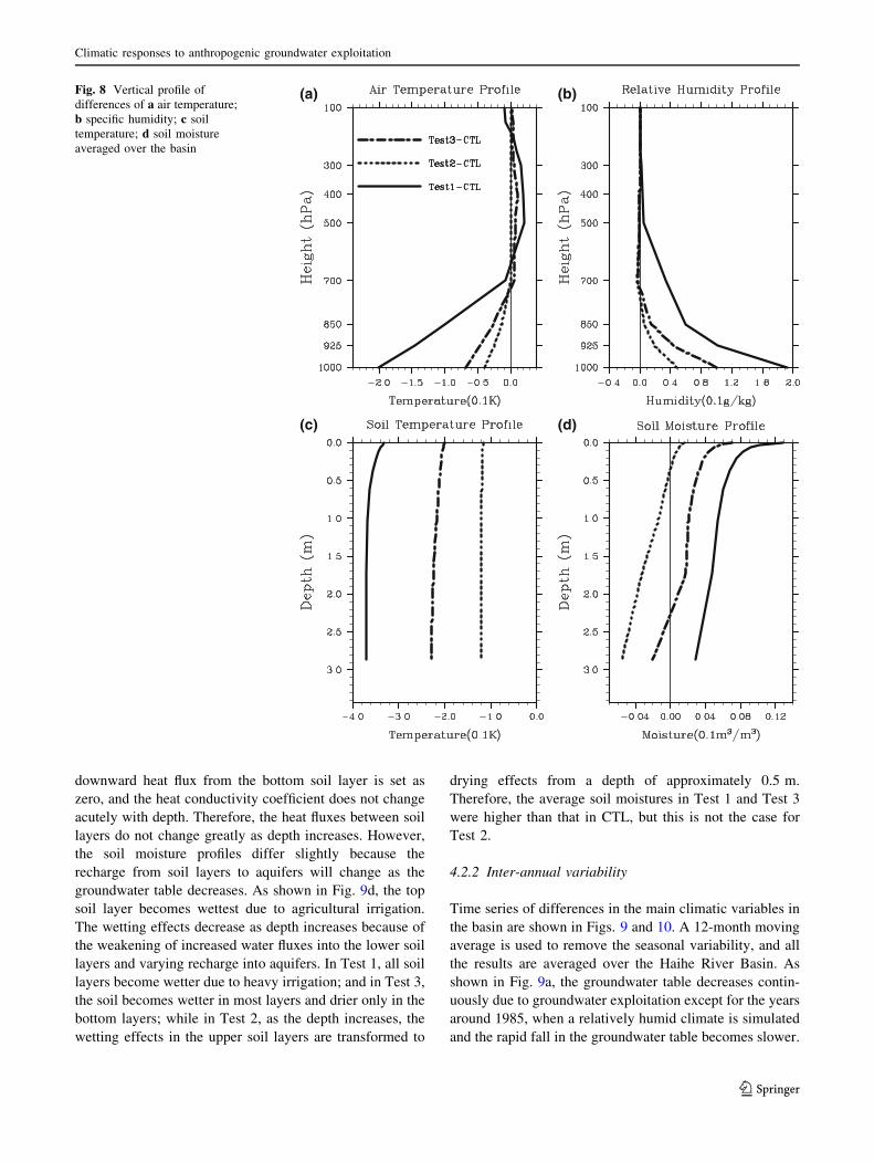
downward heat flux from the bottom soil layer is set as
zero, and the heat conductivity coefficient does not change
acutely with depth. Therefore, the heat fluxes between soil
layers do not change greatly as depth increases. However,
the soil moisture profiles differ slightly because the
recharge from soil layers to aquifers will change as the
groundwater table decreases. As shown in Fig. 9d, the top
soil layer becomes wettest due to agricultural irrigation.
The wetting effects decrease as depth increases because of
the weakening of increased water fluxes into the lower soil
layers and varying recharge into aquifers. In Test 1, all soil
layers become wetter due to heavy irrigation; and in Test 3,
the soil becomes wetter in most layers and drier only in the
bottom layers; while in Test 2, as the depth increases, the
wetting effects in the upper soil layers are transformed to
drying effects from a depth of approximately 0.5 m.
Therefore, the average soil moistures in Test 1 and Test 3
were higher than that in CTL, but this is not the case for
Test 2.
4.2.2 Inter-annual variability
Time series of differences in the main climatic variables in
the basin are shown in Figs. 9 and 10. A 12-month moving
average is used to remove the seasonal variability, and all
the results are averaged over the Haihe River Basin. As
shown in Fig. 9a, the groundwater table decreases contin-
uously due to groundwater exploitation except for the years
around 1985, when a relatively humid climate is simulated
and the rapid fall in the groundwater table becomes slower.
(a)
(c) (d)
(b)Fig. 8 Vertical profile of
differences of a air temperature;
b specific humidity; c soil
temperature; d soil moisture
averaged over the basin
Climatic responses to anthropogenic groundwater exploitation
123

By the end of the simulation period, the groundwater table
in the basin has decreased by about 5, 2.5 and 3.6 m,
respectively, for the three exploitation tests. As more water
is consumed from the land surface, evapotranspiration
increases by an average of 0.15, 0.03 and 0.07 mm/day for
the three tests. As shown in Fig. 9b, the evapotranspiration
differences increase slightly with the time, except for
during the years around 1985, when the differences in
evapotranspiration are lower. A similarly increasing trend
is also observed in differences between other moisture-
related variables, such as in the soil moisture, precipitation
and latent flux, indicating that the wetting effects on the
land surface caused by the process of groundwater
exploitation and consumption are strengthened, especially
after 1985.
In Fig. 9c, the total runoff changes by 0.035, -0.01 and
0.02 mm/day on average for Tests 1, 2 and 3 respectively.
Similar changes also appear for total soil moisture in
Fig. 9d, which changes by 0.005, -0.003 and 0.002 m3/m3
in the basin.
As shown in Fig. 9e, f, greater total precipitation and
convective precipitation are also observed in the basin in
Tests 1, 2 and 3. Specifically, the total precipitation
increases by 0.12, 0.003 and 0.03 mm/day on average,
while the convective precipitation increases by 0.09, 0.002
and 0.02 mm/day in Tests 1, 2 and 3, respectively. This
increased convective precipitation accounts for a large
proportion of the total increase in precipitation.
A slight strengthening of the cooling trend is detected
along with the wetting effects. As shown in Fig. 10a, by the
end of the simulation period, the average soil temperature
differences in the basin are -0.6, -0.18 and -0.35 K in
Tests 1, 2 and 3, respectively. Similar changes are observed
in the 2 m air temperature. In Fig. 10b, the average dif-
ferences are -0.28, -0.07 and -0.13 K in Tests 1, 2 and 3,
respectively, which are slightly lower than the soil tem-
perature differences because the 2 m air temperature is
more easily influenced by other factors, such as wind,
humidity and sensible heat, when compared to the tem-
perature of the soil surface in CLM3.5.
The cooling and wetting effects at the land surface, due
to groundwater exploitation and consumption, are also
reflected by changes in sensible heat and latent heat fluxes
(Fig. 10c, d). Specifically, in Tests 1, 2 and 3, the sensible
heat flux decreased by -3.3, -0.6 and -1.5 W/m2, while
the latent heat flux increased by 3.5, 1.1 and 1.9 W/m2,
(a) (b)
(c)
(e)
(d)
(f)
Fig. 9 Time series of differences of a groundwater table; b evapotranspiration; c total runoff; d soil moisture; e total precipitation; f convective
precipitation averaged over the basin
J. Zou et al.
123

respectively. The greater change in latent heat flux than in
sensible heat flux indicates that more energy is transferred
into the atmosphere via the phase transition of water.
Similar changes are also observed in the atmospheric
temperature and moisture patterns at 850 hPa over the
basin (Fig. 10e, f). The air temperature decreased by about
0.1, 0.02 and 0.05 K on average in Tests 1, 2 and 3, while
the specific humidity increased by about 0.06, 0.01 and
0.03 g/kg, respectively.
As presented above, the anthropogenic groundwater
exploitation and consumption removes a large amount of
water from underground and redistributes it across the land
surface of the basin. This redistribution process changes the
local distribution of land water and further affects the
regional water cycle by means of atmospheric circulation.
Table 4 shows the mean land water budget for the basin.
The positive values represent water input into the land
column and negative values the water output from the
column. Due to the continuous groundwater exploitation,
the land water storage in both exploitation tests decreases
more rapidly than that in the CTL. The decreased amount
of land water storage in Test 2 is nearly half that in Test 1,
corresponding to their different water demands. Most of the
land water exploited is dissipated through increased
evapotranspiration, and a large proportion of the increasing
moisture flux into the atmosphere returns to the land sur-
face via increased local precipitation. The wetting of the
top soil layer and decrease of the groundwater table also
changes the runoff generation in both exploitation tests.
Increased runoff is generated in Test 1, while the runoff in
Test 2 and Test 3 decreases slightly because of reduced
irrigation. Additionally, because of the exploitation of river
water (Qs) and the reduction of wastewater returned to the
(a) (b)
(c) (d)
(e) (f)
Fig. 10 Time series of differences of a soil temperature; b 2 m air temperature; c latent heat; d sensible heat; e air temperature at 850 hPa;
f specific humidity at 850 hPa averaged over the basin
Table 4 Multi-year averaged land water budget in the basin
Test 1 Test 2 Test 3 CTL
Pre (mm/year) 602.9 558.1 570.0 556.6
ET (mm/year) -589.5 -547.7 -557.2 -534.7
Rt (mm/year) -60.2 -45.8 -54.7 -48.8
Qs (mm/year) 43.0 25.1 35.8 0
Wr (mm/year) -12.1 -6.1 -10.1 0
Wt (mm/year) -44.2 -26.6 -35.5 -7.2
Pre: precipitation; ET: evapotranspiration; Rt: total runoff; Qs: water
volume pumped from rivers nearby; Wr: wastewater returned to rivers
from industrial and domestic use; Wt: land water storage changes in
the column. The positive values mean the water flux flowing into grid
columns, and the negative values mean the flux flowing out from grid
columns
Climatic responses to anthropogenic groundwater exploitation
123
rivers (Wr), the water transport from the land column into
the rivers in both exploitation tests is also less than that in
natural states with no human disturbances, which may lead
to a reduction of river discharge into the sea.
4.2.3 Seasonal variability
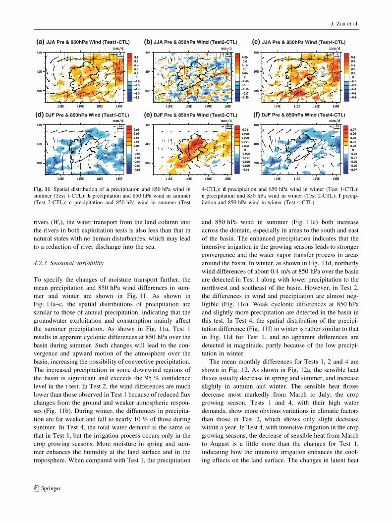
To specify the changes of moisture transport further, the
mean precipitation and 850 hPa wind differences in sum-
mer and winter are shown in Fig. 11. As shown in
Fig. 11a–c, the spatial distributions of precipitation are
similar to those of annual precipitation, indicating that the
groundwater exploitation and consumption mainly affect
the summer precipitation. As shown in Fig. 11a, Test 1
results in apparent cyclonic differences at 850 hPa over the
basin during summer. Such changes will lead to the con-
vergence and upward motion of the atmosphere over the
basin, increasing the possibility of convective precipitation.
The increased precipitation in some downwind regions of
the basin is significant and exceeds the 95 % confidence
level in the t test. In Test 2, the wind differences are much
lower than those observed in Test 1 because of reduced flux
changes from the ground and weaker atmospheric respon-
ses (Fig. 11b). During winter, the differences in precipita-
tion are far weaker and fall to nearly 10 % of those during
summer. In Test 4, the total water demand is the same as
that in Test 1, but the irrigation process occurs only in the
crop growing seasons. More moisture in spring and sum-
mer enhances the humidity at the land surface and in the
troposphere. When compared with Test 1, the precipitation
and 850 hPa wind in summer (Fig. 11c) both increase
across the domain, especially in areas to the south and east
of the basin. The enhanced precipitation indicates that the
intensive irrigation in the growing seasons leads to stronger
convergence and the water vapor transfer process in areas
around the basin. In winter, as shown in Fig. 11d, northerly
wind differences of about 0.4 m/s at 850 hPa over the basin
are detected in Test 1 along with lower precipitation to the
northwest and southeast of the basin. However, in Test 2,
the differences in wind and precipitation are almost neg-
ligible (Fig. 11e). Weak cyclonic differences at 850 hPa
and slightly more precipitation are detected in the basin in
this test. In Test 4, the spatial distribution of the precipi-
tation difference (Fig. 11f) in winter is rather similar to that
in Fig. 11d for Test 1, and no apparent differences are
detected in magnitude, partly because of the low precipi-
tation in winter.
The mean monthly differences for Tests 1, 2 and 4 are
shown in Fig. 12. As shown in Fig. 12a, the sensible heat
fluxes usually decrease in spring and summer, and increase
slightly in autumn and winter. The sensible heat fluxes
decrease most markedly from March to July, the crop
growing season. Tests 1 and 4, with their high water
demands, show more obvious variations in climatic factors
than those in Test 2, which shows only slight decrease
within a year. In Test 4, with intensive irrigation in the crop
growing seasons, the decrease of sensible heat from March
to August is a little more than the changes for Test 1,
indicating how the intensive irrigation enhances the cool-
ing effects on the land surface. The changes in latent heat
(a) (b) (c)
(f)(e)(d)
Fig. 11 Spatial distribution of a precipitation and 850 hPa wind in
summer (Test 1-CTL); b precipitation and 850 hPa wind in summer
(Test 2-CTL); c precipitation and 850 hPa wind in summer (Test
4-CTL); d precipitation and 850 hPa wind in winter (Test 1-CTL);
e precipitation and 850 hPa wind in winter (Test 2-CTL); f precip-
itation and 850 hPa wind in winter (Test 4-CTL)
J. Zou et al.
123
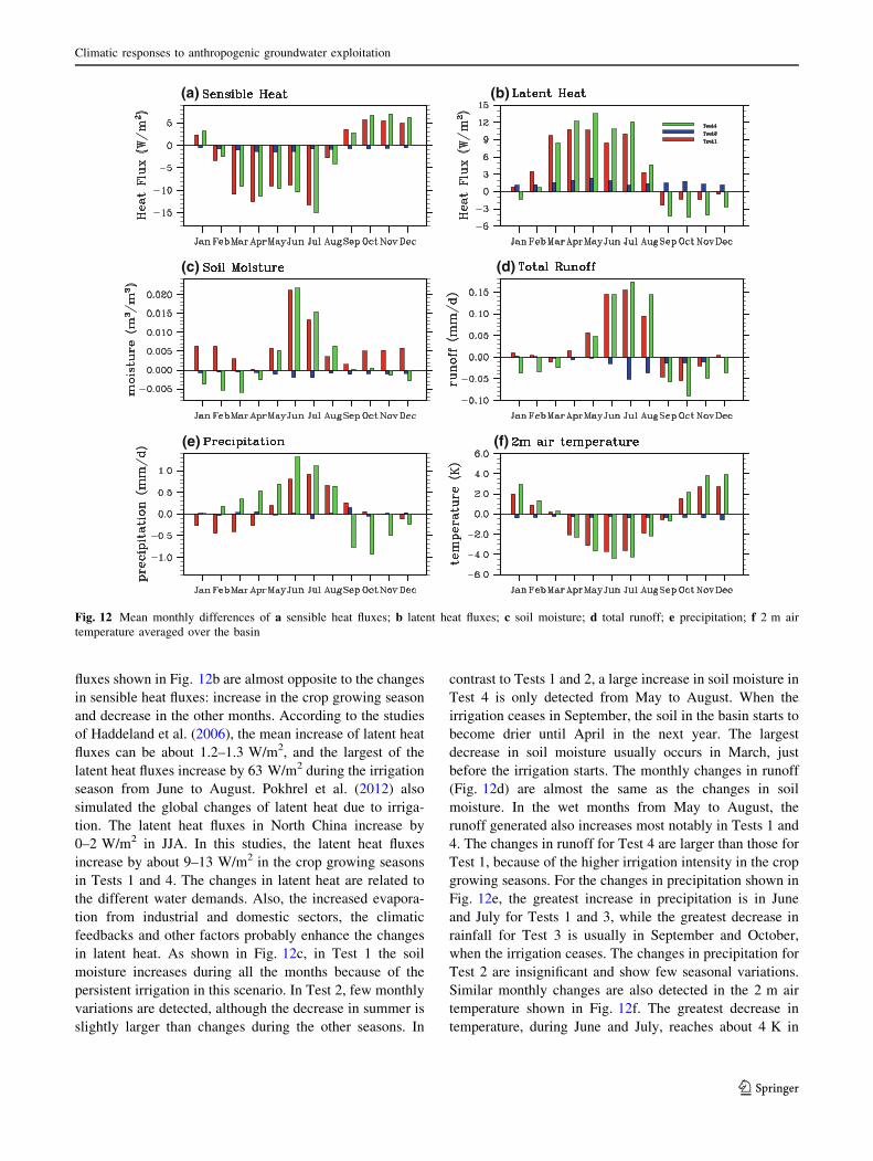
fluxes shown in Fig. 12b are almost opposite to the changes
in sensible heat fluxes: increase in the crop growing season
and decrease in the other months. According to the studies
of Haddeland et al. (2006), the mean increase of latent heat
fluxes can be about 1.2–1.3 W/m2, and the largest of the
latent heat fluxes increase by 63 W/m2 during the irrigation
season from June to August. Pokhrel et al. (2012) also
simulated the global changes of latent heat due to irriga-
tion. The latent heat fluxes in North China increase by
0–2 W/m2 in JJA. In this studies, the latent heat fluxes
increase by about 9–13 W/m2 in the crop growing seasons
in Tests 1 and 4. The changes in latent heat are related to
the different water demands. Also, the increased evapora-
tion from industrial and domestic sectors, the climatic
feedbacks and other factors probably enhance the changes
in latent heat. As shown in Fig. 12c, in Test 1 the soil
moisture increases during all the months because of the
persistent irrigation in this scenario. In Test 2, few monthly
variations are detected, although the decrease in summer is
slightly larger than changes during the other seasons. In
contrast to Tests 1 and 2, a large increase in soil moisture in
Test 4 is only detected from May to August. When the
irrigation ceases in September, the soil in the basin starts to
become drier until April in the next year. The largest
decrease in soil moisture usually occurs in March, just
before the irrigation starts. The monthly changes in runoff
(Fig. 12d) are almost the same as the changes in soil
moisture. In the wet months from May to August, the
runoff generated also increases most notably in Tests 1 and
4. The changes in runoff for Test 4 are larger than those for
Test 1, because of the higher irrigation intensity in the crop
growing seasons. For the changes in precipitation shown in
Fig. 12e, the greatest increase in precipitation is in June
and July for Tests 1 and 3, while the greatest decrease in
rainfall for Test 3 is usually in September and October,
when the irrigation ceases. The changes in precipitation for
Test 2 are insignificant and show few seasonal variations.
Similar monthly changes are also detected in the 2 m air
temperature shown in Fig. 12f. The greatest decrease in
temperature, during June and July, reaches about 4 K in
(a)
(c)
(b)
(d)
(e) (f)
Fig. 12 Mean monthly differences of a sensible heat fluxes; b latent heat fluxes; c soil moisture; d total runoff; e precipitation; f 2 m air
temperature averaged over the basin
Climatic responses to anthropogenic groundwater exploitation
123

Tests 1 and 4, and about 0.5 K in Test 2. The temperature
increases in winter in Tests 1 and 4, but by a smaller
magnitude than the increases in summer.
4.3 Separation of indirect climatic responses
in the local basin
The following discussions on the changes in the land sur-
face of the basin are based on two assumptions. (1) All
simulation results have only uniform systematic errors and
can be described as the sum of real values plus the sys-
tematic errors, so that the differences between any two
simulation tests have no systematic errors. (2) The total
changes in each land-surface variable due to the ground-
water exploitation process can be linearly divided into the
direct changes without considering local climate changes
plus the indirect changes from climatic feedbacks. The
direct changes in the local basin are defined as:
Direct Changes ¼ Roff-EX � Roff-CTL; ð9Þ
where Roff-EX is the result of off-line tests with groundwater
exploitation driven by the climate output of the on-line
control simulation; Roff-CTL is the result of the control off-
line test without any exploitation. The indirect changes
from climatic feedbacks are regarded as the total changes
minus the direct changes, and are given by:
Indirect Changes
¼ Ron-EX � Ron-CTLð Þ � Roff -EX � Roff -CTL
� �
¼ Ron-EX � Roff-EX
� �� Ron-CTL � Roff -CTL
� �; ð10Þ
where Ron-EX is the result of on-line tests with groundwater
exploitation; Ron-CTL is the result of control on-line tests
without any exploitation. According to Eq. (9), the indirect
changes can also be seen as the sum of climatic feedbacks,
Ron-EX - Roff-EX, minus the balanced status differences of
off-line and on-line tests, Ron-CTL - Roff-CTL. Although the
climate system is highly non-linear, the differences
between total changes and direct changes reflect the roles
of climatic response to some extent at least.
Unlike within the basin, in regions surrounding the basin
there are no differences among off-line tests because they
have the same climatic forcing. As a result, the total cli-
matic changes in on-line tests are determined completely
from indirect climatic feedbacks due to groundwater
exploitation and consumption in the basin, and cannot be
further separated and are therefore not discussed here.
The mean direct changes and indirect climatic feedback
in the basin are shown in Table 5. The direct changes in
land-surface variables without climatic feedback account
for less than 40 % of total changes in Test 1, indicating the
climatic feedback is stronger in the land-surface variables
of the basin. For Test 2, which has weaker climatic
responses, the proportions of direct changes are greater
than in Test 1. When compared with the direct changes for
the two exploitation tests, the changes in Test 2 are
approximately 30–50 % of those in Test 1. These findings
indicate that the direct changes of variables in land surface
are closely and linearly related to the differences in their
water demand if local indirect climatic feedback is not
considered. The indirect climatic feedback differs to a
greater degree than the direct feedback for both tests, and
the indirect changes of some variables in Test 1 are much
more than 2 or 3 times greater than the changes in Test 2.
For example, the direct changes in absorbed solar radiation
at the land surface are almost equal in the two tests because
they have the same radiation forcing, but the indirect
changes from climatic feedbacks in Test 1 are more than 10
times greater than the changes in Test 2. The differences in
direct and indirect changes in the two tests can be attrib-
uted to the high nonlinearity of the climate system. The
climatic responses due to anthropogenic groundwater
exploitation change nonlinearly as the water demand
increases in the basin. The stronger climatic feedback in
Test 1 causes wetting and cooling effects in the sur-
rounding regions outside the basin, while in Test 2 half of
the water is consumed as in Test 1, resulting in weaker
changes in heat fluxes from the land surface that are unable
to strongly affect the atmosphere over the basin, leading to
weaker climatic feedbacks. The weaker feedbacks increase
the proportion of direct changes in total changes in the
basin, and are not able to induce apparent differences in the
climatology of the regions surrounding the basin.
5 Conclusions and discussion
In this study, a simple conceptual scheme of groundwater
exploitation and consumption is developed and incorpo-
rated into the regional climate model RegCM4. The Haihe
Table 5 Mean direct and indirect changes of land surface variables
Test 1 Test 2
Direct Indirect Direct Indirect
Evp (mm/day) 0.048 0.106 0.020 0.018
Rt (mm/day) 0.006 0.028 -0.002 -0.006
Qsoi (m3/m3) -0.0004 0.0049 -0.0009 -0.0021
T2m (K) -0.084 -0.200 -0.043 -0.031
Tsoi (K) -0.157 -0.214 -0.076 -0.045
Fsa (W/m2) -0.012 -0.659 -0.011 -0.058
SH (W/m2) -0.730 -2.538 -0.277 -0.383
LH (W/m2) 1.409 3.071 0.594 0.529
Evp evapotranspiration, Rt total runoff, Qsoi total soil moisture, T2m
2m air temperature, Tsoi soil temperature, Fsa absorbed solar radia-
tion, SH sensible heat flux, LH latent heat flux
J. Zou et al.
123

River Basin in Northern China is chosen as the study
domain because of the severe over-exploitation of
groundwater resource in that region. Four on-line simula-
tion tests (Test 1, 2, 3 and 4) with different water demands
and a control test (CTL) without exploitation are conducted
to detect changes in regional climate and sensitivities of the
climatic responses to different water demands. Three off-
line tests are also conducted to specify the roles of direct
changes and indirect climatic feedback in the basin.
The main conclusions of this study are as follows. (1)
The process of groundwater exploitation and consumption
in the Haihe River Bain causes a rapid decrease in local
land water storage, and causes increasing wetting and
cooling effects at the local land surface and in the lower
troposphere of the basin. Increased precipitation,
enhanced evapotranspiration, and decreased 2 m air tem-
perature are detected in the basin during the four on-line
exploitation tests. The changes in these climatic factors
are usually most marked in summer. The 2 m air tem-
perature can decrease most strongly, by 3–4 K, during the
growing season in tests using the estimated water demand
in 2000. (2) The process of reallocation of land water
resources in the basin also induced climate changes in the
regions surrounding the basin. More precipitation is
detected, especially in downwind regions of the prevailing
westerly, because more moisture is transferred into the
atmosphere through stronger convective activities in the
basin in summer. In addition, decreased air temperatures
in the land surface and lower troposphere are detected to
the western regions outside of the basin. (3) The changes
of climatic variables in the exploitation tests are posi-
tively related to their different water demands. The rela-
tionship is usually non-linear because of the climatic
responses. The changes in variables in Test 2, which has
half the water demand of Test 1, are far weaker than
those in Test 1. (4) If the changes in climatic forcing are
not considered, the direct changes in the land-surface
variables of the two exploitation tests in the local basin
are approximately linearly related to their different water
demands. However, the indirect climatic feedback of the
two tests is highly nonlinear and enlarges the differences
between Tests 1 and 2.
The results of our study demonstrate some possible
climatic responses to water resource exploitation and
consumption; however, it is important to note that there are
many assumptions in this study. Accordingly, future stud-
ies should be conducted to improve our present findings.
For example, the framework of groundwater exploitation
and consumption processes is highly simplified and shows
some major differences when compared with the actual
processes.
In RegCM4/CLM3.5, the river routing model is not
included and the water quantity in reservoirs or lakes
cannot be specified. We assume the pumped streamflow
is only from local runoff generated in the groundwater
exploitation scheme. Therefore, the absence of river
routing and reservoir operation greatly limits the
strength of our scheme, and probably leads to less land-
surface water and more pumped groundwater when the
quantity of exploited water is estimated. Moreover, the
estimated water demand and allocation proportion of
water consumed in this study also introduces many
uncertainties. The division of evaporation from the
industrial and domestic water consumption sectors is
subjective, and greatly simplifies the process of waste-
water being re-used before flowing into the sea. For
irrigation consumption, we do not consider water
transport losses or other forms of dissipation. The
approach of adding irrigation water to effective rainfall
does not consider soil moisture deficit.
There are many uncertainties in the exploitation simu-
lations which will need addressing and, when compared
with the observations, the simulations by the exploitation
tests still contain significant biases: for example, discrep-
ancies in the spatial distribution of the groundwater table.
The simulated climatic changes over regions outside the
Haihe River Basin may be not correct, because this study
only considers the process of local water exploitation and
consumption in the Haihe River Basin. In fact, this
groundwater exploitation process is common over many
regions in North China.
Nevertheless, this paper is designed to lead to discus-
sions of changes due to groundwater exploitation and
sensitivities of climatic responses to different water
demands in the Haihe River Basin, not develop or promote
the simulation abilities of the model. The cooling effects
caused by groundwater exploitation and consumption
might promote a warmer temperature bias and shallower
groundwater table in the study domain simulated by Reg-
CM4, but the enhanced precipitation in the exploitation
tests also increases the wetter bias of the model. Therefore,
it is difficult to confirm that the exploitation tests promote
the model’s simulation abilities because the changes are
not significant for some variables and are likely artifacts of
errors of a model which does not consider some more
important processes beyond the anthropogenic perturba-
tions of water resources.
To improve the groundwater exploitation scheme in
future studies, effort should be directed at addressing the
river routing process, the water quantity in reservoirs or
lakes, the lateral flow of groundwater in a basin, reasonable
approximation of the water consumption sector, and so on.
Also, water demand should be estimated more accurately in
China or even at a global scale so that the effects of
groundwater exploitation and consumption can be evalu-
ated over a wider domain.
Climatic responses to anthropogenic groundwater exploitation
123

Acknowledgments This study is supported by the National Basic
Research Program of China under Grants 2010CB428403 and
2010CB951001, the National Natural Science Foundation of China
under Grant 91125016, and the Chinese Academy of Sciences Stra-
tegic Priority Research Program (Grant No. XDA05110102). We
would like to thank Xiangjun Tian, Xiaoduo Pan and Yingdong Yu
for their assistance with data processing and interpretation of the
results, and the executive editor Edwin K. Schneider and the two
anonymous reviewers for constructive comments and suggestions
which have helped us in improving the paper.
References
Adegoke JO, Pielke RA, Eastman J, Mahmood R, Hubbard KG
(2003) Impact of irrigation on midsummer surface fluxes and
temperature under dry synoptic conditions: a regional atmo-
spheric model study of the US High Plain. Mon Weather Rev
131(3):556–564
Biggs TW, Scott CA, Gaur A, Venot JP, Chase T, Lee E (2008)
Impacts of irrigation and anthropogenic aerosols on the water
balance, heat fluxes, and surface temperature in a river basin.
Water Resour Res 44:W12415. doi:10.1029/2008WR006847
Boucher O, Myhre G, Myhre A (2004) Direct human influence of
irrigation on atmospheric water vapor and climate. Clim Dyn
22(6):597–603
Chen X, Hu Q (2004) Groundwater influences on soil moisture and
surface evaporation. J Hydrol 297:285–300
Chen F, Xie Z (2010) Effects of interbasin water transfer on regional
climate: a case study of the Middle Route of the South-to-North
Water Transfer Project in China. J Geophys Res 115:D11112.
doi:10.1029/2009JD012611
DeAngelis A, Dominguez F, Fan Y, Robock A, Kutsu MD, Robinson
D (2010) Evidence of enhanced precipitation due to irrigation
over the Great Plains of the United States. J Geophys Res
115:D15115. doi:10.1029/2010JD013892
Dickinson R, Seller AH, Kennedy P (1993) Biosphere Atmosphere
Transfer Scheme (BATS) version 1e as coupled to the NCAR
Community Climate Model, Tech. Rep. National Center for
Atmospheric Research, Boulder, Colorado, USA
Doll P, Hoffmann-Dobrev H, Portmann FT, Siebert S, Eicker A,
Rodell M (2012) Impact of water withdrawals from groundwater
and surface water on continental water storage variations.
J Geodyn 59–60:143–156. doi:10.1016/j.jog.2011.05.001
Douglas EM, Beltran-Przekurat A, Niyogi D, Pielke A Sr, Voro-
smarty CJ (2009) The impact of agricultural intensification and
irrigation on land-atmosphere interactions and Indian monsoon
precipitation—a mesoscale modeling perspective. Global Planet
Change 67(1–2):117–128. doi:10.1016/j.gloplacha.2008.12.007
Gao X, Shi Y, Zhang D, Wu J, Giorgi F, Ji Z, Wang Y (2012)
Uncertainties in monsoon precipitation projections over China:
results from two high-resolution RCM simulations. Clim Res
52:213–226. doi:10.3354/cr01084
Giorgi F, Anyah RO (2012) The road towards RegCM4. Clim Res
52:3–6. doi:10.3354/cr01089
Giorgi F, Marinucci M, Bates G, Canio G (1993) Development of a
second-generation regional climate model (RegCM2): part II.
Convective processes and assimilation of lateral boundary
conditions. Mon Weather Rev 121:2814–2832
Giorgi F, Coppola E, Solmon F, Mariotti L, Sylla MB, Bi X, Elguindi
N, Diro GT, Nair V, Giuliani G, Turuncoglu UU, Cozzini S,
Guttler I, O’Brien TA, Taufik AB, Shalaby A, Zakey AS, Steiner
AL, Stordal F, Sloan LC, Brankovic C (2012) RegCM4: model
description and preliminary tests over multiple CORDEX
demains. Clim Res 52:7–29. doi:10.3354/cr01018
Grell G, Dudhia JJ, Stauffer D (1994) A description of the fifth-
generation Penn State/NCAR Mesoscale Model (MM5), Tech.
Rep. National Center for Atmospheric Research, Boulder,
Colorado, USA
Haddeland I, Lettenmaier DP, Skaugen T (2006) Effects of irrigation
on the water and energy balances of the Colorado and Mekong
river basins. J Hydrol 324:210–223
Hanasaki N, Kanae S, Oki T, Masuda K, Motoya K, Shirakawa N,
Shen Y, Tanaka K (2008) An integrated model for the
assessment of global water resources—Part 1: model description
and input meteorological forcing. Hydrol Earth Syst Sci
12:1007–1025
Harding KJ, Snyder PK (2012) Modeling the atmospheric response to
irrigation in the Great Plains. Part I: general impacts on precipi-
tation and the energy budget. J Hydrometeorol 13:1667–1686
Jia Y, Ding Y, Wang H, Zhou Z, Qiu Y, Niu C (2012) Attribution of
water resources evolution in the highly water-stressed Hai River
Basin of China. Water Resour Res 48:W02513. doi:10.1029/
2010WR009275
Kollet SJ, Zlotnik VA (2003) Stream depletion predictions using
pumping tests data from a heterogeneous stream-aquifer system
(a case study from the Great Plains, USA). J Hydrol
281(1–2):96–114
Konikow LF, Kendy E (2005) Groundwater depletion: a global
problem. Hydrogeol J 13(1):317–320
Kueppers LM, Snyder MA (2012) Influence of irrigated agricultural
on diurnal surface energy and water fluxes, surface climate, and
atmospheric circulation in California. Clim Dyn 38:1017–1029
Kueppers LM, Snyder MA, Sloan LC (2007) Irrigation cooling effect:
regional climate forcing by land-use change. Geophys Res Lett
34:L03703. doi:10.1029/2006GL028679
Kustu MD, Fan Y, Robock A (2010) Large-scale water cycle
perturbation due to irrigation pumping in the US High Plains: a
synthesis of observed streamflow changes. J Hydrol
390(1–4):222–244
Liang F, Tao S, Wei J, Bueh C (2011) Variation in summer rainfall in
North China during the period 1956–2007 and links with
atmospheric circulation. Adv Atmos Sci 28(2):363–374. doi:10.
1007/s00376-010-9220-2
Lobell DB, Bonfils CJ, Kueppers LM, Snyder MA (2008) Irrigation
cooling effect on temperature and heat index extremes. J Geo-
phys Res 35:L09705. doi:10.1029/2008GL034145
Mao X, Ni J, Guo Y (2000) A case study on characteristics of
wastewater effluents in accelerated economic growth areas. Acta
Sci Circumst 20(2):219–224 (in Chinese)
Moore N, Rojstaczer S (2002) Irrigation’s influence on precipitation:
Texas High Plains, USA. Geophys Res Lett 29(16):1755. doi:10.
1029/2002GL014940
Niu G, Yang Z, Dickinson RE, Gulden LE (2005) A simple
TOPMODEL-based runoff parameterization (SIMTOP) for use
in global climate models. J Geophys Res 110:D21106. doi:10.
1029/2005JD006111
Niu G, Yang Z, Dickinson RE, Gulden LE, Su H (2007) Development
of a simple groundwater model for use in climate models and
evaluation with Gravity Recovery and Climate Experiment data.
J Geophys Res 112:D07103. doi:10.1029/2006JD007522
Oleson KW, Dai Y, Bonan G, Bosilovich M, Dickinson R, Dirmeyer
P, Hoffman F, Houser P, Levis S, Niu G, Thornton P,
Vertenstein M, Yang Z, Zeng X (2004) Technical description
of the Community Land Model (CLM), Tech. Rep. National
Center for Atmospheric Research, Boulder, Colorado, USA
Oleson KW, Niu G, Yang Z, Lawrence DM, Thornton PE, Lawrence
PJ, Stockli R, Dickinson RE, Bonan GB, Levis S, Dai A, Qian T
(2008) Improvements to the Community Land Model and their
impact on the hydrological cycle. J Geophys Res 113:G01021.
doi:10.1029/2007JG000563
J. Zou et al.
123

Ozdogan M, Rodell M, Beaudoing HK, Toll D (2010) Simulating the
effects of irrigation over the United States in a land surface
model based on satellite-derived agricultural data. J Hydromete-
orol 11:171–184
Ozturk T, Altinsoy H, Turkes M, Kurnaz ML (2012) Simulation of
temperature and precipitation climatology for the Central Asia
CORDEX domain using RegCM4.0. Clim Res 52:63–76. doi:10.
3354/cr01082
Pokhrel Y, Hanasaki N, Koirala S, Cho J, Kim H, Yeh PJ-F, Kanae S,
Oki T (2012) Incorporating anthropogenic water regulation
modules into a land surface model. J Hydrometeorol 13:255–269
Puma MJ, Cook BI (2010) Effects of irrigation on global climate
during the 20th century. J Geophys Res 115:D16120. doi:10.
1029/2010JD014122
Qian Y, Huang M, Yang B, Berg LK (2013) A modeling study of
irrigation effects on surface fluxes and land-air-cloud interac-
tions in the Southern Great Plains. J Hydrometeorol 14:700–712
Ren X (2007) Water resource assessment of Haihe River Basin. China
Water Power Press, Beijing (in Chinese)
Ren L, Wang M, Li C, Zhang W (2002) Impacts of human activity on
river runoff in the northern area of China. J Hydrol 261:204–217
Rijsberman FR (2006) Water scarcity: fact or fiction? Agric Water
Manag 80:5–22
Sacks WJ, Cook BI, Buenning N, Levis S, Helkowski JH (2009)
Effects of global irrigation on the near-surface climate. Clim
Dyn 33(2):159–175
Saeed F, Hagemann S, Jacob D (2009) Impact of irrigation on the
South Asian summer monsoon. Geophys Res Lett 36:L20711.
doi:10.1029/2009GL040625
Sha T, Roy AD, Qureshi AS, Wang J (2003) Sustaining Asia’s
groundwater boom: an overview of issues and evidence. Nat
Resour Forum 27:130–141
Shiklomanov IA (2000) Appraisal and assessment of world water
resources. Water Int 25:11–32
Szilagyi J (1999) Streamflow depletion investigations in the Repub-
lican River basin: Colorado, Nebraska, and Kansas. J Environ
Syst 27(3):251–263
Szilagyi J (2001) Indentifying cause of declining flows in the
Republican River. J Water Resour Plan Manag 127(4):244–253
Tian X, Xie Z, Dai A (2008) A land surface soil moisture data
assimilation system based on the dual-UKF method and the
Community Land Model. J Geophys Res 113:D14127. doi:10.
1029/2007JD009650
Wang A, Zeng X (2011) Sensitivities of terrestrial water cycle
simulations to the variations of precipitation and air temperature
in China. J Geophys Res 116:D02107. doi:10.1029/
2010JD014659
Xia J, Chen D (2001) Water problem and opportunities in hydrolog-
ical Sciences in China. Hydrol Sci J 46(6):907–922
Xia J, Zhang Y (2008) Water security in north China and counter-
measure to climate change and human activity. Phys Chem Earth
33:359–363
Xie Z, Yuan F, Duan Q, Zheng J, Liang M, Chen F (2007) Regional
parameter estimation of the VIC land surface model: method-
ology and application to river basins in China. J Hydrometeorol
8(3):447–468
Xu Y, Mo X, Cai Y, Li X (2004) Analysis on groundwater table
drawdown by land use and quest for sustainable water use in the
Hebei Plain in China. Agric Water Manag 75:38–53
Yang Y, Tian F (2009) Abrupt change of runoff and its major driving
factors in Haihe River Catchment, China. J Hydrol 374:373–383
Yuan X, Xie Z, Zheng J, Tian X, Yang Z (2008) Effects of water table
dynamics on regional climate: a case study over East Asian
monsoon area. J Geophys Res 113:D21112. doi:10.1029/
2008JD0101
Zhang F, Wang D, Qiu B (1987) China agricultural phenology atlas.
Science Press, Beijing (in Chinese)
Climatic responses to anthropogenic groundwater exploitation
123