Part IB Physics B

Classical Dynamics

S.F. Gull

University of Cambridge

Department of Physics

Michaelmas Term 2011 and Lent Term 2012

Synopsis

This course builds on the ideas introduced in Part IA, using the machinery of vector calculustaught in Part IA Mathematics. The main areas covered are orbits, rigid body dynamics,normal modes and continuum mechanics (elasticity and fluids).

Newtonian mechanics, frames of reference. Review of Part IA mechanics: many-particle system, internal and external forces and energy. Central forces, motion in a plane.Non-inertial frames, rotating frames, centrifugal and Coriolis forces. Examples.

Orbits. Effective potential and radial motion, bound and unbound orbits. Inverse-squarelaw orbits, circular and elliptic, Kepler’s laws. Escape velocity, transfer orbits, gravitationalslingshot. Hyperbolic orbits, angle of scattering, repulsive force. Two-body problem, reducedmass. General features of three-body problem.Brief treatment of tidal effects in gravitationalsystems.

Rigid body dynamics. Instantaneous motion of a rigid body, angular velocity and angularmomentum, moment of inertia tensor, principal axes and moments. Rotational energy, inertiaellipsoid. Euler’s equations, free precession of a symmetrical top, space and body frequencies.Forced precession, gyroscopes.

Introduction to Lagrangian mechanics. Generalised coordinates. Hamilton’s principleand Lagrange’s equations. Symmetries and conservation laws. Conservation of the Hamilto-nian for time-independent systems.

Normal modes. Analysis of many-particle system in terms of normal modes. Degrees offreedom, matrix notation, zero-frequency and degenerate modes. Continuum limit, waveequation. Standing waves, energy and normal modes. Motion in three dimensions, modes ofmolecules.

Elasticity. Hooke’s law, Young’s modulus, Poisson’s ratio. Bulk modulus, shear modulus,stress tensor, principal stresses. strain tensor. Elastic energy. Torsion of cylinder. Bending ofbeams, bending moment, boundary conditions. Euler strut. Brief treatment of elastic waves.Energy flow in waves.

Fluid dynamics. Continuum fields, material derivatives, relation to particle paths andstreamlines. Mass conservation, incompressibility. Convective derivative and equation ofmotion. Bernoulli’s theorem, applications. Velocity potential, applications: sources and sinks;flow past a sphere and cylinder; vortices; Magnus effect. Viscosity, Couette and Poiseuilleflow. Reynolds number, lamina and turbulent flow.

1

Books

Classical Mechanics, Barger V D and Olsson M G (McGaw-Hill, 1995).

Classical Mechanics, Kibble T W B and Berkshire F H (Imperial College 2004).

Principles of Dynamics, Greenwood D T (Prentice & Hall 1988).

Mechanics, Landau L D and Lifshitz E M, (Pergamon, 1976)

For elasticity

Lectures on Physics, Feynman R P, Leighton R B and Sands S L (Addison Wesley 1964).

Theory of Elasticity, Landau L D and Lifshitz E M,( Pergamon, 1976)

For fluids

Fluid Dynamics for Physicists, Faber T E, (Cambridge, 1995).

Lectures on Physics, Feynman R P, Leighton R B and Sands S L (Addison Wesley 1964).

2

Contents

1 Mathematics — Review 6

1.1 Coordinate systems . . . . . . . . . . . . . . . . . . . . . . . . . . . . . . . . . 61.2 Vectors . . . . . . . . . . . . . . . . . . . . . . . . . . . . . . . . . . . . . . . . 61.3 Matrices . . . . . . . . . . . . . . . . . . . . . . . . . . . . . . . . . . . . . . . 7

1.3.1 Geometrical view . . . . . . . . . . . . . . . . . . . . . . . . . . . . . . 71.3.2 Orthogonal matrices . . . . . . . . . . . . . . . . . . . . . . . . . . . . 71.3.3 Tensors . . . . . . . . . . . . . . . . . . . . . . . . . . . . . . . . . . . 71.3.4 Eigen vectors, eigen values . . . . . . . . . . . . . . . . . . . . . . . . . 81.3.5 Quadratic forms . . . . . . . . . . . . . . . . . . . . . . . . . . . . . . . 8

1.4 Rotations . . . . . . . . . . . . . . . . . . . . . . . . . . . . . . . . . . . . . . 8

2 Coordinate systems 10

2.1 Fixed frames . . . . . . . . . . . . . . . . . . . . . . . . . . . . . . . . . . . . . 102.2 Frames in relative motion . . . . . . . . . . . . . . . . . . . . . . . . . . . . . 102.3 Rotating frames . . . . . . . . . . . . . . . . . . . . . . . . . . . . . . . . . . . 11

3 Mechanics — Review 13

3.1 Overall motion . . . . . . . . . . . . . . . . . . . . . . . . . . . . . . . . . . . 133.2 Moments . . . . . . . . . . . . . . . . . . . . . . . . . . . . . . . . . . . . . . . 133.3 Choice of origin . . . . . . . . . . . . . . . . . . . . . . . . . . . . . . . . . . . 143.4 Energy . . . . . . . . . . . . . . . . . . . . . . . . . . . . . . . . . . . . . . . . 143.5 Galilean transformation . . . . . . . . . . . . . . . . . . . . . . . . . . . . . . 15

3.5.1 Momentum . . . . . . . . . . . . . . . . . . . . . . . . . . . . . . . . . 153.5.2 Angular momentum . . . . . . . . . . . . . . . . . . . . . . . . . . . . 153.5.3 Energy . . . . . . . . . . . . . . . . . . . . . . . . . . . . . . . . . . . . 15

4 Orbits 16

4.1 Radial equation . . . . . . . . . . . . . . . . . . . . . . . . . . . . . . . . . . . 164.2 Power-law force . . . . . . . . . . . . . . . . . . . . . . . . . . . . . . . . . . . 16

4.2.1 Nearly circular orbits . . . . . . . . . . . . . . . . . . . . . . . . . . . . 164.3 Inverse square orbits . . . . . . . . . . . . . . . . . . . . . . . . . . . . . . . . 17

4.3.1 Shape of orbit . . . . . . . . . . . . . . . . . . . . . . . . . . . . . . . . 174.3.2 Time in orbit . . . . . . . . . . . . . . . . . . . . . . . . . . . . . . . . 18

4.4 Unbound inverse square orbits . . . . . . . . . . . . . . . . . . . . . . . . . . . 18

5 Rigid body dynamics 20

5.1 J and ω . . . . . . . . . . . . . . . . . . . . . . . . . . . . . . . . . . . . . . . 205.1.1 Principal axes . . . . . . . . . . . . . . . . . . . . . . . . . . . . . . . . 215.1.2 Elementary properties . . . . . . . . . . . . . . . . . . . . . . . . . . . 21

5.2 Free motion . . . . . . . . . . . . . . . . . . . . . . . . . . . . . . . . . . . . . 215.3 Poinsot’s treatment . . . . . . . . . . . . . . . . . . . . . . . . . . . . . . . . . 22

5.3.1 Symmetrical top . . . . . . . . . . . . . . . . . . . . . . . . . . . . . . 225.3.2 Asymmetrical top . . . . . . . . . . . . . . . . . . . . . . . . . . . . . . 23

5.4 Euler’s equations . . . . . . . . . . . . . . . . . . . . . . . . . . . . . . . . . . 235.4.1 Symmetrical top . . . . . . . . . . . . . . . . . . . . . . . . . . . . . . 245.4.2 Asymmetrical top . . . . . . . . . . . . . . . . . . . . . . . . . . . . . . 25

5.5 Lagrange . . . . . . . . . . . . . . . . . . . . . . . . . . . . . . . . . . . . . . . 25

3

5.5.1 Force-free motion . . . . . . . . . . . . . . . . . . . . . . . . . . . . . . 265.5.2 With external couple . . . . . . . . . . . . . . . . . . . . . . . . . . . . 265.5.3 Precession . . . . . . . . . . . . . . . . . . . . . . . . . . . . . . . . . . 275.5.4 Nutation . . . . . . . . . . . . . . . . . . . . . . . . . . . . . . . . . . . 27

6 Normal modes 29

6.1 Basic theory . . . . . . . . . . . . . . . . . . . . . . . . . . . . . . . . . . . . . 296.1.1 Equations of Motion . . . . . . . . . . . . . . . . . . . . . . . . . . . . 296.1.2 Oscillations . . . . . . . . . . . . . . . . . . . . . . . . . . . . . . . . . 306.1.3 Orthogonality . . . . . . . . . . . . . . . . . . . . . . . . . . . . . . . . 316.1.4 Energy . . . . . . . . . . . . . . . . . . . . . . . . . . . . . . . . . . . . 32

6.2 Extensions . . . . . . . . . . . . . . . . . . . . . . . . . . . . . . . . . . . . . . 336.2.1 Masses different . . . . . . . . . . . . . . . . . . . . . . . . . . . . . . . 336.2.2 Extended masses . . . . . . . . . . . . . . . . . . . . . . . . . . . . . . 34

6.3 Many parameter systems . . . . . . . . . . . . . . . . . . . . . . . . . . . . . . 346.3.1 Equations of motion . . . . . . . . . . . . . . . . . . . . . . . . . . . . 346.3.2 Normal modes . . . . . . . . . . . . . . . . . . . . . . . . . . . . . . . . 346.3.3 Energy . . . . . . . . . . . . . . . . . . . . . . . . . . . . . . . . . . . . 35

7 Elasticity — Fundamentals 37

7.1 Basic ideas . . . . . . . . . . . . . . . . . . . . . . . . . . . . . . . . . . . . . . 377.2 Stress . . . . . . . . . . . . . . . . . . . . . . . . . . . . . . . . . . . . . . . . 377.3 Strain . . . . . . . . . . . . . . . . . . . . . . . . . . . . . . . . . . . . . . . . 387.4 General elastic modulus . . . . . . . . . . . . . . . . . . . . . . . . . . . . . . 397.5 Isotropic materials . . . . . . . . . . . . . . . . . . . . . . . . . . . . . . . . . 39

7.5.1 Bulk modulus . . . . . . . . . . . . . . . . . . . . . . . . . . . . . . . . 397.5.2 Shear modulus . . . . . . . . . . . . . . . . . . . . . . . . . . . . . . . 397.5.3 Other forms . . . . . . . . . . . . . . . . . . . . . . . . . . . . . . . . . 40

7.6 Voigt notation . . . . . . . . . . . . . . . . . . . . . . . . . . . . . . . . . . . . 417.7 Work, energy . . . . . . . . . . . . . . . . . . . . . . . . . . . . . . . . . . . . 41

7.7.1 dW is a ‘perfect differential’ . . . . . . . . . . . . . . . . . . . . . . . . 427.7.2 Integration of W . . . . . . . . . . . . . . . . . . . . . . . . . . . . . . 42

8 Elasticity — Applications 43

8.1 Simple examples . . . . . . . . . . . . . . . . . . . . . . . . . . . . . . . . . . 438.2 Bending of beams . . . . . . . . . . . . . . . . . . . . . . . . . . . . . . . . . . 438.3 Euler strut . . . . . . . . . . . . . . . . . . . . . . . . . . . . . . . . . . . . . . 45

8.3.1 Equilibrium analysis . . . . . . . . . . . . . . . . . . . . . . . . . . . . 458.3.2 Energy . . . . . . . . . . . . . . . . . . . . . . . . . . . . . . . . . . . . 45

9 Elastic waves 47

9.1 Basic theory . . . . . . . . . . . . . . . . . . . . . . . . . . . . . . . . . . . . . 479.1.1 F and u . . . . . . . . . . . . . . . . . . . . . . . . . . . . . . . . . . . 479.1.2 τ and F . . . . . . . . . . . . . . . . . . . . . . . . . . . . . . . . . . . 479.1.3 τ , e and u . . . . . . . . . . . . . . . . . . . . . . . . . . . . . . . . . . 47

9.2 Plane waves . . . . . . . . . . . . . . . . . . . . . . . . . . . . . . . . . . . . . 489.2.1 Transverse waves . . . . . . . . . . . . . . . . . . . . . . . . . . . . . . 489.2.2 Longitudinal waves . . . . . . . . . . . . . . . . . . . . . . . . . . . . . 489.2.3 Relative velocities . . . . . . . . . . . . . . . . . . . . . . . . . . . . . . 48

4

9.2.4 Fluids . . . . . . . . . . . . . . . . . . . . . . . . . . . . . . . . . . . . 499.2.5 General u(r) . . . . . . . . . . . . . . . . . . . . . . . . . . . . . . . . . 49

9.3 Waves on a plate . . . . . . . . . . . . . . . . . . . . . . . . . . . . . . . . . . 509.4 Waves on rods . . . . . . . . . . . . . . . . . . . . . . . . . . . . . . . . . . . . 50

9.4.1 Torsional waves . . . . . . . . . . . . . . . . . . . . . . . . . . . . . . . 509.4.2 Transverse waves . . . . . . . . . . . . . . . . . . . . . . . . . . . . . . 50

9.5 Propagation, impedance . . . . . . . . . . . . . . . . . . . . . . . . . . . . . . 519.6 Reflection of waves — Not for Examination . . . . . . . . . . . . . . . . . . . 52

9.6.1 Normal incidence . . . . . . . . . . . . . . . . . . . . . . . . . . . . . . 529.6.2 Oblique incidence . . . . . . . . . . . . . . . . . . . . . . . . . . . . . . 529.6.3 Oblique incidence — qualitative summary . . . . . . . . . . . . . . . . 539.6.4 Rayleigh waves . . . . . . . . . . . . . . . . . . . . . . . . . . . . . . . 54

5

1 Mathematics — Review

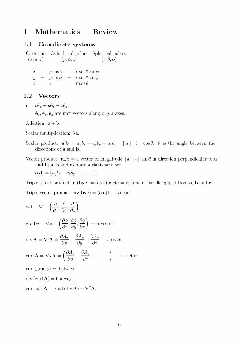
1.1 Coordinate systems

Cartesian Cylindrical polars Spherical polars(x, y, z) (ρ, φ, z) (r, θ, φ)

x = ρ cosφ = r sin θ cosφy = ρ sinφ = r sin θ sinφz = z = r cos θ

1.2 Vectors

r = xex + yey + zez.

ex, ey, ez are unit vectors along x, y, z axes.

Addition: a + b.

Scalar multiplication: λa.

Scalar product: a·b = axbx + ayby + azbz = | a | | b | cos θ. θ is the angle between thedirections of a and b.

Vector product: a×××××b = a vector of magnitude |a | | b | sin θ in direction perpendicular to a

and b; a, b and a×××××b are a right-hand set.

a×××××b = (aybz − azby, . . . , . . .).

Triple scalar product: a·(b×××××c) = (a×××××b)·c etc = volume of parallelepiped from a, b and c.

Triple vector product: a×××××(b×××××c) = (a.c)b− (a.b)c.

del = ∇ =

(

∂

∂x,∂

∂y,∂

∂z

)

.

gradφ = ∇φ =

(

∂φ

∂x,∂φ

∂y,∂φ

∂z

)

— a vector.

divA = ∇·A =∂Ax∂x

+∂Ay∂y

+∂Az∂z

— a scalar.

curlA = ∇×××××A =

(

∂Az∂y− ∂Ay

∂z, . . . , . . .

)

— a vector.

curl (gradφ) = 0 always.

div (curlA) = 0 always.

curl curlA = grad (divA)−∇2A.

6

1.3 Matrices

1.3.1 Geometrical view

Linear relation between vectors: r′ = Mr. Two situations:

1. Linear transformation of space (rotation, deformation etc of an object). Point P at r ina body is displaced to r′. Columns of M ≡ where unit vectors along the original axesare moved to.

2. Change of axes. r′ and r refer to the same vector (same magnitude and direction inspace) in new and old coordinate systems. Columns of M ≡ old e’s (unit vectors alongaxes) in new coordinates; those of M−1 ≡ new e’s in old coordinates.

1.3.2 Orthogonal matrices

preserve orthogonality of axes; scalar products of different columns are zero. If in additionthe scalar product of any column with itself is 1, then

=

1 . .. 1 .. . 1

= I, (. = 0)

or M′M = I, or M−1 = M′ [M′ is the transpose of M].

1.3.3 Tensors

Given a = Kb, with a and b vectors and K a matrix, a tensor is the relationship between a

and b thought of as magnitudes and directions in space without regard to components wrtspecific axes [a physicist’s view — see IB Maths for a formal treatment; we need to enlargeit later]. For given (3D) axes, K needs 9 numbers

ai =∑

j

Kijbj.

The tensor is usually written Kij.Rotate axes by M, giving a′ = Ma, b′ = Mb. Then

M−1a′ = KM−1b′,

ora′ = MKM−1

︸ ︷︷ ︸b′.

≡ K′

The tensor is the relationship expressed by K and K′, which are physically equivalent, thoughtheir components are different.

Ex. 1 Stress in a material. b = vector area of a surface within the material, a = force acrossthat surface; a is linear with (‘proportional to’) b though not necessarily parallel to it. The‘proportionality’ is the stress tensor.

7

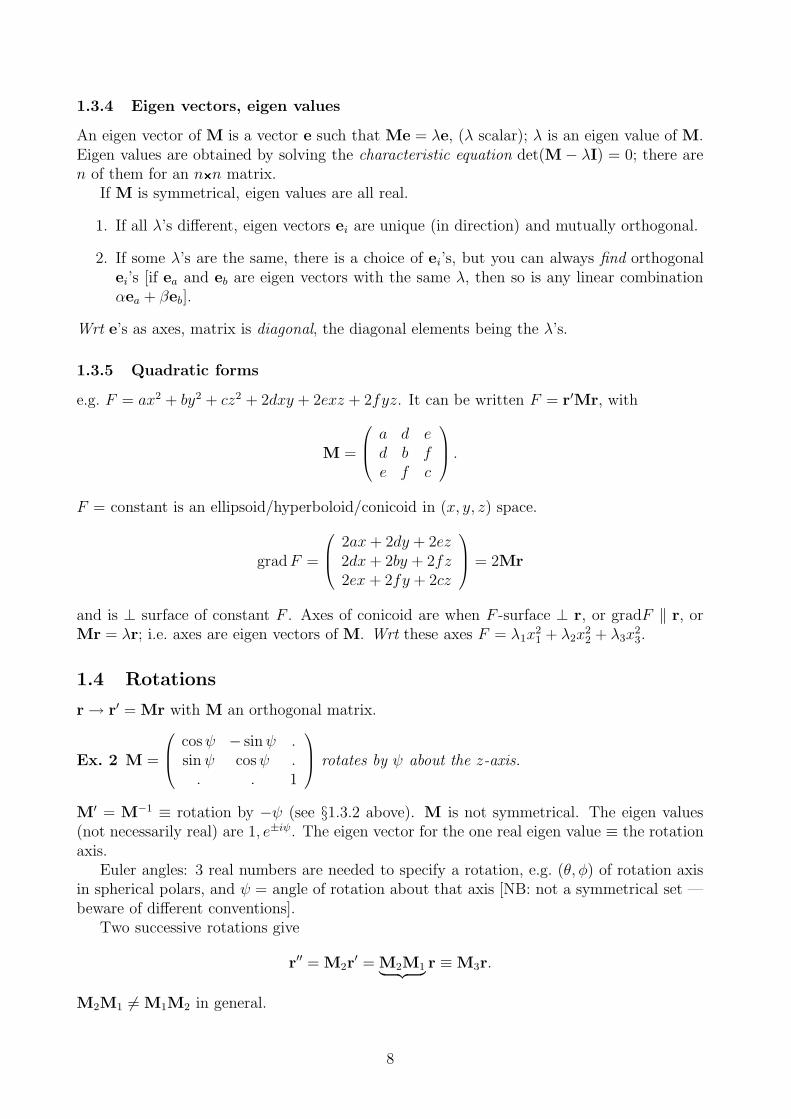
1.3.4 Eigen vectors, eigen values

An eigen vector of M is a vector e such that Me = λe, (λ scalar); λ is an eigen value of M.Eigen values are obtained by solving the characteristic equation det(M− λI) = 0; there aren of them for an n×××××n matrix.

If M is symmetrical, eigen values are all real.

1. If all λ’s different, eigen vectors ei are unique (in direction) and mutually orthogonal.

2. If some λ’s are the same, there is a choice of ei’s, but you can always find orthogonalei’s [if ea and eb are eigen vectors with the same λ, then so is any linear combinationαea + βeb].

Wrt e’s as axes, matrix is diagonal, the diagonal elements being the λ’s.

1.3.5 Quadratic forms

e.g. F = ax2 + by2 + cz2 + 2dxy + 2exz + 2fyz. It can be written F = r′Mr, with

M =

a d ed b fe f c

.

F = constant is an ellipsoid/hyperboloid/conicoid in (x, y, z) space.

gradF =

2ax+ 2dy + 2ez2dx+ 2by + 2fz2ex + 2fy + 2cz

= 2Mr

and is ⊥ surface of constant F . Axes of conicoid are when F -surface ⊥ r, or gradF ‖ r, orMr = λr; i.e. axes are eigen vectors of M. Wrt these axes F = λ1x

21 + λ2x

22 + λ3x

23.

1.4 Rotations

r→ r′ = Mr with M an orthogonal matrix.

Ex. 2 M =

cosψ − sinψ .sinψ cosψ .. . 1

rotates by ψ about the z-axis.

M′ = M−1 ≡ rotation by −ψ (see §1.3.2 above). M is not symmetrical. The eigen values(not necessarily real) are 1, e±iψ. The eigen vector for the one real eigen value ≡ the rotationaxis.

Euler angles: 3 real numbers are needed to specify a rotation, e.g. (θ, φ) of rotation axisin spherical polars, and ψ = angle of rotation about that axis [NB: not a symmetrical set —beware of different conventions].

Two successive rotations give

r′′ = M2r′ = M2M1

︸ ︷︷ ︸r ≡M3r.

M2M1 6= M1M2 in general.

8

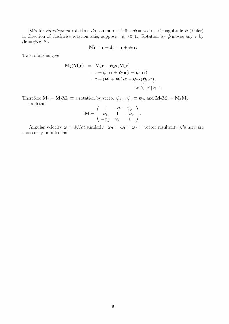
M’s for infinitesimal rotations do commute. Define ψ= vector of magnitude ψ (Euler)in direction of clockwise rotation axis; suppose | ψ | 1. Rotation by ψ moves any r bydr = ψ×××××r. So

Mr = r + dr = r +ψ×××××r.

Two rotations give

M2(M1r) = M1r +ψ2×××××(M1r)

= r +ψ1×××××r +ψ2×××××(r +ψ1×××××r)

= r + (ψ1 +ψ2)×××××r +ψ2×××××(ψ1×××××r)︸ ︷︷ ︸

.

≈ 0, |ψ | 1

Therefore M3 = M2M1 ≡ a rotation by vector ψ2 +ψ1 ≡ ψ3, and M2M1 = M1M2.In detail

M =

1 −ψz ψyψz 1 −ψx−ψy ψx 1

.

Angular velocity ω = dψ/dt similarly. ω3 = ω1 + ω2 = vector resultant. ψ’s here arenecessarily infinitesimal.

9

2 Coordinate systems

2.1 Fixed frames

In Cartesians, the equation of motion of a particle is

mr = F; or mx = Fx etc.

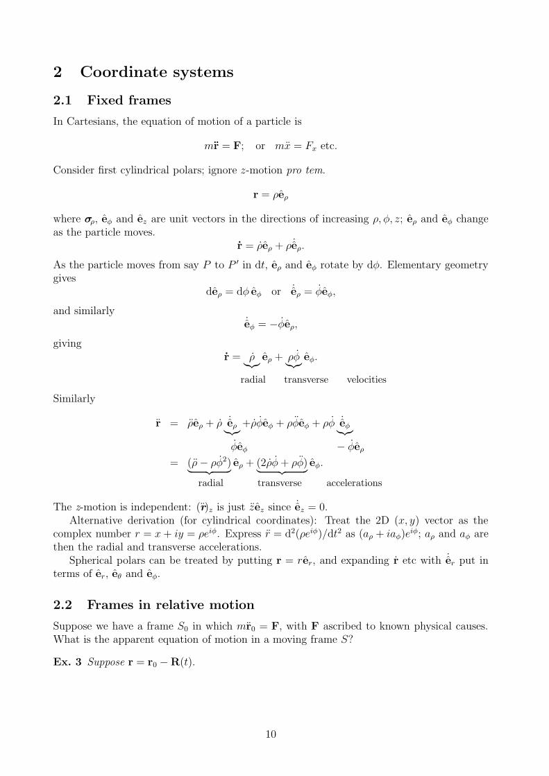
Consider first cylindrical polars; ignore z-motion pro tem.

r = ρeρ

where σρ, eφ and ez are unit vectors in the directions of increasing ρ, φ, z; eρ and eφ changeas the particle moves.

r = ρeρ + ρ ˙eρ.

As the particle moves from say P to P ′ in dt, eρ and eφ rotate by dφ. Elementary geometrygives

deρ = dφ eφ or ˙eρ = φeφ,

and similarly˙eφ = −φeρ,

givingr = ρ

︸︷︷︸eρ + ρφ

︸︷︷︸eφ.

radial transverse velocities

Similarly

r = ρeρ + ρ ˙eρ︸︷︷︸

+ρφeφ + ρφeφ + ρφ ˙eφ︸︷︷︸

φeφ − φeρ= (ρ− ρφ2)

︸ ︷︷ ︸eρ + (2ρφ+ ρφ)

︸ ︷︷ ︸eφ.

radial transverse accelerations

The z-motion is independent: (r)z is just zez since ˙ez = 0.Alternative derivation (for cylindrical coordinates): Treat the 2D (x, y) vector as the

complex number r = x + iy = ρeiφ. Express r = d2(ρeiφ)/dt2 as (aρ + iaφ)eiφ; aρ and aφ are

then the radial and transverse accelerations.Spherical polars can be treated by putting r = rer, and expanding r etc with ˙er put in

terms of er, eθ and eφ.

2.2 Frames in relative motion

Suppose we have a frame S0 in which mr0 = F, with F ascribed to known physical causes.What is the apparent equation of motion in a moving frame S?

Ex. 3 Suppose r = r0 −R(t).

10

Axes remain parallel and t = t0 (as always in classical physics).

r = r0 − R.

For the special case R = 0 (i.e. steady motion between frames), mr = mr0 = F, i.e. the sameequation of motion (Galilean transformation).

For general R,mr = mr0 −mR

or the apparent force in S includes both the actual force (mr0, as in S0) and a fictitious force−mR. Fictitious forces are

1. associated with accelerated frames, and

2. proportional to mass.

Question: Is gravity a fictitious force? Answer (according to Einstein and general relativity):Yes — space is curved, i.e. non-linear, and equivalent to acceleration in some sense.

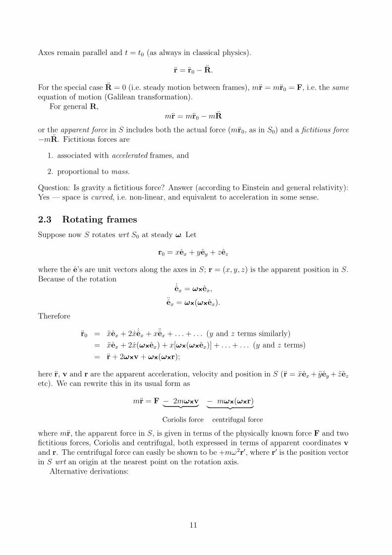
2.3 Rotating frames

Suppose now S rotates wrt S0 at steady ω. Let

r0 = xex + yey + zez

where the e’s are unit vectors along the axes in S; r = (x, y, z) is the apparent position in S.Because of the rotation

˙ex = ω×××××ex,

¨ex = ω×××××(ω×××××ex).

Therefore

r0 = xex + 2x ˙ex + x¨ex + . . .+ . . . (y and z terms similarly)

= xex + 2x(ω×××××ex) + x[ω×××××(ω×××××ex)] + . . .+ . . . (y and z terms)

= r + 2ω×××××v + ω×××××(ω×××××r);

here r, v and r are the apparent acceleration, velocity and position in S (r = xex+ yey + zezetc). We can rewrite this in its usual form as

mr = F − 2mω×××××v︸ ︷︷ ︸

− mω×××××(ω×××××r)︸ ︷︷ ︸

Coriolis force centrifugal force

where mr, the apparent force in S, is given in terms of the physically known force F and twofictitious forces, Coriolis and centrifugal, both expressed in terms of apparent coordinates v

and r. The centrifugal force can easily be shown to be +mω2r′, where r′ is the position vectorin S wrt an origin at the nearest point on the rotation axis.

Alternative derivations:

11

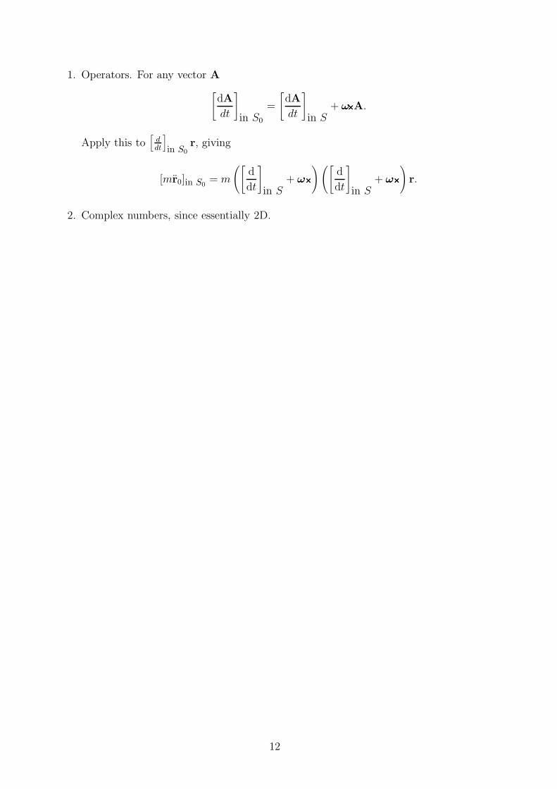
1. Operators. For any vector A

[

dA

dt

]

in S0

=

[

dA

dt

]

in S+ ω×××××A.

Apply this to[ddt

]

in S0

r, giving

[mr0]in S0= m

([

d

dt

]

in S+ ω×××××

)([

d

dt

]

in S+ ω×××××

)

r.

2. Complex numbers, since essentially 2D.

12

3 Mechanics — Review

Development from Newton’s Laws.mara = Fa;

a = 1, N for the a’th of N particles. A rigid body is a special case.

3.1 Overall motion

∑

a

mara =∑

a

Fa =∑

a

Fa0 +∑

a

∑

b

Fab

where Fa0 is the external force on particle a and Fab is the force on a due to b. SinceFab = −Fba by Newton’s 3rd Law, the

∑

a

∑

b term above sums to zero.Put M =

∑

ama and MR =∑

amara. R is the position of the Centre of Mass. Then

MR =∑

a

Fa0 = F0

i.e. the Centre of Mass moves as if it were a particle of mass M acted upon by the resultantexternal force F0.

In terms of momentumpa = Fa; P = F0

with P = total momentum.

3.2 Moments

Def n. 1 Couple, torque: G = r×××××F.

Def n. 2 Angular momentum: J = r×××××p.

Since pa = Fa, ∑

a

ra×××××pa =∑

a

ra×××××Fa.

Expand RHS:RHS =

∑

a

ra×××××Fa0 +∑

a

∑

b

ra×××××Fab

︸ ︷︷ ︸

.

∑∑

a<b

(ra − rb)×××××Fab︸ ︷︷ ︸

= 0

The latter term is zero since Fab is assumed to be along the line between a and b.The LHS for one particle is

Ja =d

dt(ra×××××pa) = ra×××××pa

︸ ︷︷ ︸+ra×××××pa.

zero, since mr = p

For the system of particles

J =∑

a

Ja =∑

a

ra×××××pa = RHS =∑

a

ra×××××Fa0 = G0;

G0 is the resultant G from all external forces.

13

3.3 Choice of origin

Suppose we move the origin by a constant a, giving new coordinates r′ with r = r′ +a. Thenr = r′ and §3.1 unaffected. What about J? For one particle Ja = J′

a + a×××××pa, or for thesystem

J = J′ +∑

a

a×××××pa = J′ + a×××××P,

i.e. J depends on the choice of origin unless P = 0.

Def n. 3 Intrinsic angular momentum: J in the frame in which P = 0 (zero-momentum,or Centre of Mass frame). It is independent of origin.

Similarly G = G′ + a×××××F.

3.4 Energy

Def n. 4 Work done: force ××××× distance moved ‖ force = change in energy.

For a single particleF · dr = mr · dr = m r · r

︸︷︷︸dt

d

dt(12r · r)

orF · dr = d(1

2mv2).

Def n. 5 Kinetic energy: T ≡ 12mv2.

Work done on particle = change in kinetic energy.For a system of particles

dT =∑

a

dTa =∑

a

Fa · dra

=∑

a

Fa0 · dra +∑∑

a<b

Fab · (dra − drb)

where we have used Fab = −Fba. We can write the ab-term as −Fabd | ra − rb |, where Fabhas magnitude = |Fab | and is positive if force is attractive, negative if repulsive.

Def n. 6 Potential energy, internal energy: U , such that

dU =∑∑

a<b

Fab d | ra − rb | .

Note the zero of U =∫

dU is undefined. It is often taken with U = 0 with particles at infiniteseparation, giving negative U for a system of particles with attractive forces. For a rigid bodydU = 0 since | ra − rb | is fixed.

Def n. 7 Energy: E = T + U .

As defined abovedE = dT + dU =

∑

a

Fa0 · dra.

The RHS term is the work done by external forces; it can be incorporated into U if desired.

14

3.5 Galilean transformation

Go from frame S to S ′ with r = r′ + Vt; V steady; t = t′.

3.5.1 Momentum

p = p′ +mV; P = P′ +MV;

i.e. P in S and P′ in S ′ change together (or remain steady together if there if no externalforce). If P′ = 0, then S ′ is the zero-momentum or Centre of Mass frame.

3.5.2 Angular momentum

J =∑

a

(r′a + Vt)×××××(p′

a +maV).

There are 4 terms. The 4th is V×××××V = 0. The others give

J = J′ + Vt×××××P′ +∑

a

r′a×××××maV

︸ ︷︷ ︸

.

∑

a

(mar′

a)×××××V = MR′×××××V

Thus if S ′ is the zero-momentum frame, P′ = 0 and

J = J′ +MR′×××××V

︸ ︷︷ ︸.

in S intrinsic motion of C of M in S

3.5.3 Energy

T =∑

a

12mav

2a = 1

2ma(v

′

a + V) · (v′

a + V)

= T ′ +∑

a

mav′

a

︸ ︷︷ ︸

·V + 12MV 2.

(= 0, if S′ = zero-momentum frame)

orT = KE in zero-momentum frame + 1

2MV 2.

15

4 Orbits

Motion of a particle in a central force field: F ‖ r; FerF (r). Potential energy U(r); F =−dU/dr. Immediate features

1. Motion confined to the plane defined by r and v.

2. No couple from central force, therefore constant J. J is ⊥ plane of orbit. |J |= mr2φ= m× (twice rate of describing area). Kepler’s 2nd Law.

4.1 Radial equation

m(r − rφ2) = −dUdr.

Put φ = J/mr2 (J constant). Then

mr = −dUdr

+J2

mr3= −dU

′

dr

where

U ′ = effective U ≡ U +J2

2mr2.

An alternative derivation is via energy: E = U + 12m(r2 + r2φ2) = 1

2mr2 + U ′.

4.2 Power-law force

Let F = −Arn; A positive, so force is attractive; n = index, with common cases n = +1 (2DSHM) and n = −2 (gravity, electrostatics).

U ′ =Arn+1

n + 1+

J2

2mr2.

4.2.1 Nearly circular orbits

as oscillations/perturbations about r0. Taylor expansion of U ′ gives

U ′ = U ′

min + (r − r0)(

dU ′

dr

)

r0

+ 12(r − r0)2

(

d2U ′

dr2

)

r0

+ · · ·

dU ′/dr is zero at U ′

min giving

dU ′

dr= +Arn − J2

mr3= 0 at r0;

d2U ′

dr2= nArn−1 +

3J2

mr4

=(n+ 3)J2

mr40

at r0.

16

Therefore SHM equation

mr +(n+ 3)J2

mr40

(r − r0)︸ ︷︷ ︸

= 0;

1st-order Taylor of dU ′/dr

i.e. SHM about r0 with angular frequency

ωp =√n + 3

J

mr20

.

How does ωp of the perturbation compare with ωc of the circular orbit at r0? ωc = φ = J/mr20.

Therefore ωp =√n + 3ωc. The common cases are

1. n = 1. Force proportional to r, i.e. SHM. ωp = 2ωc, giving a central ellipse (Lissajousfigure).

2. n = −2. Inverse square force. ωp = ωc, giving an ellipse with a focus at r = 0 (planetaryorbit).

General n gives non-commensurate ωp and ωc and non-repeating orbits.

4.3 Inverse square orbits

F = −A/r2, U = −A/r. Minimum of U ′ is at r0 = J2/Am = radius of circular orbit of givenJ .

Energy: E = 12mr2 +

J2

2mr2︸ ︷︷ ︸

−Ar.

Ar02r2

Angular momentum: J = mr2φ.

4.3.1 Shape of orbit

We may writeJ× v = −A ˙er

since the vectors J, v and ˙er have magnitudes mr2φ, A/mr2 and φ respectively and aremutually perpendicular; the sign is obtained by inspection. Since J is constant the equationmay be integrated to give

J× v + A(er + e) = 0

where e is a vector integration constant. Taking the dot-product of this equation with r gives

J× v · r︸ ︷︷ ︸

+A(r + e · r) = 0.

= J · v × r = −J2/m

Therefore

r(1 + e · er) = r(1 + e cosφ) =J2

mA= r0. (1)

17

This is the polar equation of a conic with focus at r = 0 (Kepler’s 1st Law). The major axisis in the direction of e; e is the eccentricity: 0, <1, 1 or >1 for a circle, ellipse, parabola orhyperbola. r0 is the semi-latus-rectum, i.e. half the width at the position of the focus.

To get the energy take the scalar product of Ae = −(J× v + Aer) with itself (note thatJ and v are perpendicular)

A2e2 = J2v2 + 2J× v · er︸ ︷︷ ︸

A+ A2

= J · v × er = −J2/mr

Therefore

A2(e2 − 1) = J2(

v2 − 2A

mr

)

=2EJ2

m

where E is the total energy. The major axis of the orbit is given by

2a = r0

(1

1 + e+

1

1− e

)

=2r0

1− e2= −A

E

i.e. E = −A/2a independent of eccentricity.

4.3.2 Time in orbit

The integral of φ(t) to give φ(t) is insoluble in elementary functions. We can get the period,from the area and d(area)/dt = J/2m. To get the area, turn equation (1) into Cartesians, togive

(x+ x0

a

)2

+y2

b2= 1

witha =

r01− e2

, b =r0√

1− e2, x0 = ea.

The area is πab, so that

Period =πab

J/2m=

πr20

(1− e2)3/2

2m

(r0Am)1/2= 2π

(

ma3

A

)1/2

,

i.e. proportional to a3/2 independent of e; Kepler’s 3rd Law.

4.4 Unbound inverse square orbits

Hyperbolic orbits. They can occur with an attractive force and E positive, or a repulsiveforce and any E, e.g. between two positively charged nuclei. The algebra is similar to that ofthe ellipse with some changes of sign; e > 1. b is the impact parameter ; if the orbiting bodyis initially at infinity with positive speed, b is how close to the central body it would pass ifit were not deviated by the force.

Important results in practice are

1. J = mr2φ = mbv∞ = mrcvc where c suffix refers to the moment of closest approach.

2. Energy equation gives rc and vc in terms of b and v∞.

18

3. The asymptotes occur when r becomes infinite, i.e. 1 + e cosφ∞ = 0 in Eqn. (2).cosφ∞ = −1/e (φ∞ is between 90 and 180, say 180 − ψ∞). Geometry of er and e

gives | er + e |= tanψ∞ and the magnitudes of the two terms in Eqn. (1) give

tanψ∞ =Jv∞A

=mv2

∞b

A.

The total deviation during the traverse is 180 − 2ψ∞.

For a repulsive orbit, with force = B/r2, B positive, the angle of deviation is similarly

180 − 2 arctanmv2

∞b

B.

The angle of the symptotes can also be simply derived from the x−momentum.

19

5 Rigid body dynamics

Basic equations:

MR = F0; centre of mass moves as if it were a particle of mass M under action of theresultant external force.

J = G0; d/dt of angular momentum = total external couple.

Reminder: J and T in general frame = J and T in zero-momentum frame + contributionfrom motion of M as if a particle. In this section we consider only force-free motion in thezero-momentum frame.

5.1 J and ω

J =∑

r×××××p =∑

r×××××m(ω×××××r)

=∑

mr2ω−∑

mr(ω· r︸ ︷︷ ︸

).

ωxx + ωyy + ωzz

Therefore J is proportional to ω but not necessarily parallel to ω, i.e. a matrix/tensor rela-tionship J = Iω. In detail

JxJyJz

=

∑m(y2 + z2) −∑mxy −∑mxz−∑mxy

∑m(x2 + z2) −∑myz

−∑mxz −∑myz∑m(x2 + y2)

ωxωyωz

.

I is the Moment of Inertia matrix (or tensor).Also

T =∑ 1

2m(ω×××××r) · (ω×××××r)

=∑ 1

2mω· r×××××(ω×××××r) = 1

2ω· J.

The Moment of Inertia tensor is symmetrical. There are therefore 3 real eigen values I1

to I3 and 3 mutually perpendicular eigen vectors e1 to e3. Wrt eigen-vector axes,

I′ =

I1 . .. I2 .. . I3

.

J1 = I1ω1 etc, or

J =

I1ω1

I2ω2

I3ω3

.

T = 12(I1ω

21 + I2ω

22 + I3ω

23).

I1 to I3 are the Principal Moments of Inertia = moments of inertia in the ordinary senseabout the eigenvector axes; the eigenvector axes are called the Principal Axes. In ω-space, asurface of constant T = T (ω) is an ellipsoid, the Moment of Inertia Ellipsoid; the axes of the

ellipsoid have length ∝ I−1/2i . The ellipsoid is regarded as fixed to the body.

In ω-space,

gradT =

(

∂T

∂ω1,∂T

∂ω2,∂T

∂ω3

)

= (I1ω1, I2ω2, I3ω3) ≡ J

i.e. J is ⊥ surface of constant T at ω.

20

5.1.1 Principal axes

They are fixed to the body and must be ⊥ each other, whatever the shape of the body.Rotationally bodies come in three types

1. Spherical Tops; all I’s equal, e.g. sphere, cube. J = Iωwith a scalar I. J ‖ ω in thiscase. Rotationally the body is isotropic, with the same I about any axis.

2. Symmetrical Tops; I1 = I2 6= I3, e.g. many simple molecules. Subgroups are oblate(lens or disc shaped) and prolate (cigar shaped). e3 axis unique; e1 and e2 anywherein plane ⊥ e3.

3. Asymmetrical Tops; all three I’s different. Principal axes unique.

5.1.2 Elementary properties

1. No one Ii can be larger than the sum of the other two. Thus (wrt x, y, z along principalaxes)

I1 + I2 =∑

m(y2 + z2 + x2 + z2) = I3 + 2∑

mz2 ≥ I3.

A special case is a flat lamina, z = 0, for which I1 + I2 = I3, the Theorem of Perpen-dicular Axes.

Ex. 4 Disc, mass M , radius a.

I3 =∑

m(x2 + y2) =∫ a

02πrdr

M

πa2r2 = 1

2Ma2.

I1 = I2 = moment of inertia about a diameter = 14Ma2.

2. Theorem of Parallel axes. For I about an axis not through centre of mass, say a awayand parallel to a principal axis.

I =∑

m(r + a) · (r + a) = I0 +Ma2 + 2(∑

mr)

· a = I0 +Ma2,

since∑mr is zero when r is wrt C of M. [Vectors r etc here are all taken as 2D

projections in plane perpendicular to I axis.]

5.2 Free motion

F = 0, G = 0, i.e. an isolated body spinning freely. J is constant. What about ω? Answer istrivial if J and ω are along a principal axis. Otherwise behaviour is much more complicated:the direction of ωvaries both in space and wrt the body; for asymmetrical tops, the magnitudeof ωvaries too. The variations are called free precession, to distinguish them from the forcedprecession produced by an external couple.

The problem of handling free precession may be treated in three quite different ways:

1. Poinsot’s geometrical approach.

2. Euler’s equations = the equations of motion in a coordinate frame moving with thebody.

3. Lagrange’s appoach, which gives the equations of motion wrt fixed axes.

The 2nd and 3rd of these generalise readily to include forced motion, i.e. with external couples.

21

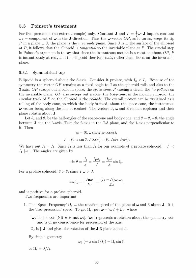
5.3 Poinsot’s treatment

For free precession (no external couple) only. Constant J and T = 12ω · J implies constant

ωJ = component of ω in the J-direction. Thus the ω-vector OP , as it varies, keeps its tipP in a plane ⊥ J; the plane is the invariable plane. Since J is ⊥ the surface of the ellipsoidat P , it follows that the ellipsoid is tangential to the invariable plane at P . The crucial stepin Poinsot’s argument is to say that since the instanteous motion is a rotation about OP , Pis instanteously at rest, and the ellipsoid therefore rolls, rather than slides, on the invariableplane.

5.3.1 Symmetrical top

Ellipsoid is a spheroid about the 3-axis. Consider it prolate, with I3 < I1. Because of thesymmetry the vector OP remains at a fixed angle to J as the spheroid rolls and also to the3-axis. OP sweeps out a cone in space, the space-cone, P tracing a circle, the herpolhode onthe invariable plane. OP also sweeps out a cone, the body-cone, in the moving ellipsoid; thecircular track of P on the ellipsoid is the polhode. The overall motion can be visualised as arolling of the body-cone, to which the body is fixed, about the space cone, the instanteousω-vector being along the line of contact. The vectors J, ω and 3 remain coplanar and theirplane rotates about J.

Let θs and θb be the half-angles of the space-cone and body-cone, and θ = θs+θb the anglebetween J and the 3-axis. Take the 2-axis in the J-3 plane, and the 1-axis perpendicular toit. Then

ω= (0, ω sin θb, ω cos θb);

J = (0, J sin θ, J cos θ) = (0, I1ω2, I3ω3).

We have put I2 = I1. Since I3 is less than I1 for our example of a prolate spheroid, | J |<I1 |ω | . The angles are given by

sin θ =J2

J=I1ω2

J=I1ω

Jsin θb.

For a prolate spheroid, θ > θb since I1ω > J .

sin θs =| J×××××ω |Jω

=(I1 − I3)ω2ω3

Jω.

and is positive for a prolate spheroid.Two frequencies are important

1. The ‘Space Frequency’ Ωs ≡ the rotation speed of the plane of ω and 3 about J. It isthe ‘free precession’ speed. To get Ωs, put ω= ‘ω3’ + Ωs , where

‘ω3’ is ‖ 3-axis [NB it is not ω3]. ‘ω3’ represents a rotation about the symmetry axisand is of no consequence for precession of the axis.

Ωs is ‖ J and gives the rotation of the J-3 plane about J.

By simple geometryω2 (= J sin θ/I1) = Ωs sin θ,

or Ωs = J/I1.

22

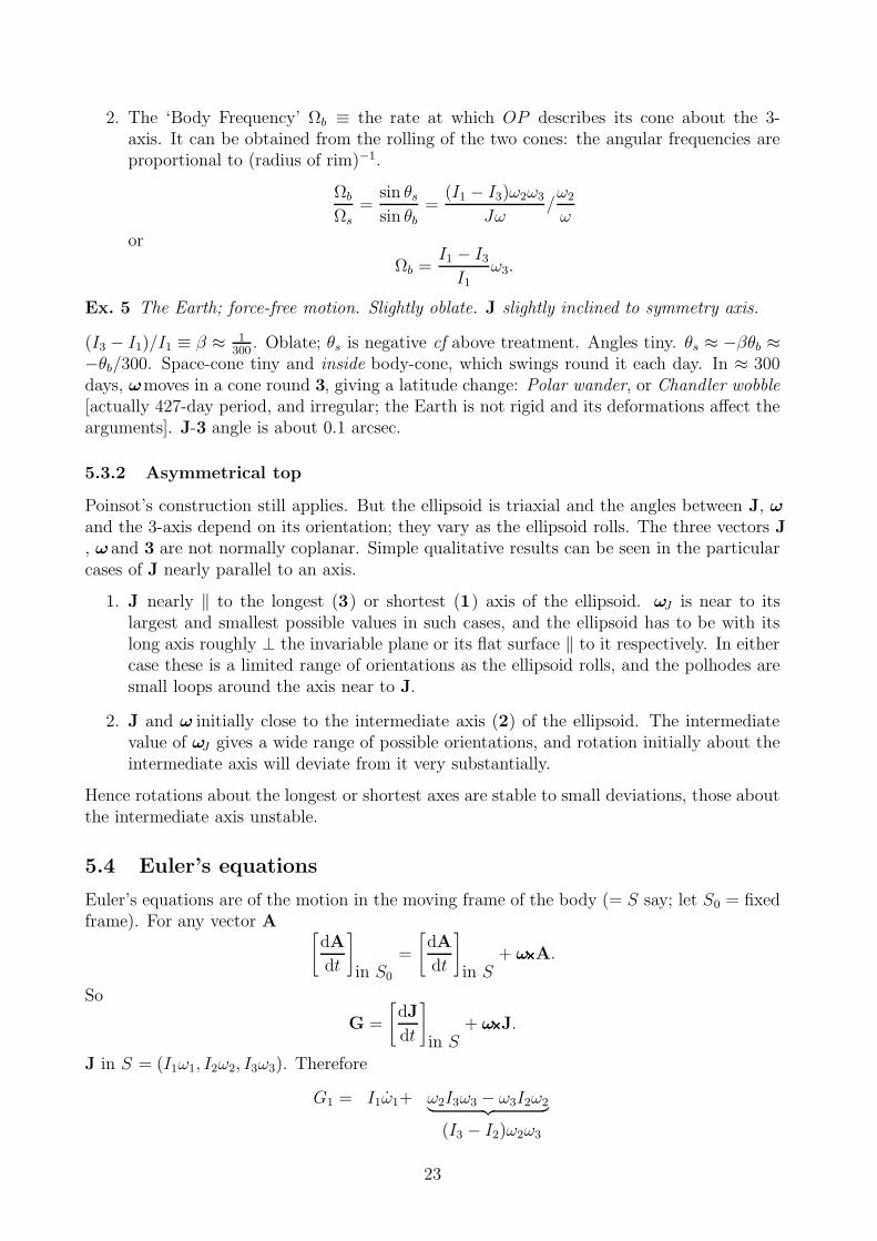
2. The ‘Body Frequency’ Ωb ≡ the rate at which OP describes its cone about the 3-axis. It can be obtained from the rolling of the two cones: the angular frequencies areproportional to (radius of rim)−1.

Ωb

Ωs

=sin θssin θb

=(I1 − I3)ω2ω3

Jω/ω2

ω

or

Ωb =I1 − I3I1

ω3.

Ex. 5 The Earth; force-free motion. Slightly oblate. J slightly inclined to symmetry axis.

(I3 − I1)/I1 ≡ β ≈ 1300

. Oblate; θs is negative cf above treatment. Angles tiny. θs ≈ −βθb ≈−θb/300. Space-cone tiny and inside body-cone, which swings round it each day. In ≈ 300days, ωmoves in a cone round 3, giving a latitude change: Polar wander, or Chandler wobble[actually 427-day period, and irregular; the Earth is not rigid and its deformations affect thearguments]. J-3 angle is about 0.1 arcsec.

5.3.2 Asymmetrical top

Poinsot’s construction still applies. But the ellipsoid is triaxial and the angles between J, ωand the 3-axis depend on its orientation; they vary as the ellipsoid rolls. The three vectors J

, ω and 3 are not normally coplanar. Simple qualitative results can be seen in the particularcases of J nearly parallel to an axis.

1. J nearly ‖ to the longest (3) or shortest (1) axis of the ellipsoid. ωJ is near to itslargest and smallest possible values in such cases, and the ellipsoid has to be with itslong axis roughly ⊥ the invariable plane or its flat surface ‖ to it respectively. In eithercase these is a limited range of orientations as the ellipsoid rolls, and the polhodes aresmall loops around the axis near to J.

2. J and ω initially close to the intermediate axis (2) of the ellipsoid. The intermediatevalue of ωJ gives a wide range of possible orientations, and rotation initially about theintermediate axis will deviate from it very substantially.

Hence rotations about the longest or shortest axes are stable to small deviations, those aboutthe intermediate axis unstable.

5.4 Euler’s equations

Euler’s equations are of the motion in the moving frame of the body (= S say; let S0 = fixedframe). For any vector A

[

dA

dt

]

in S0

=

[

dA

dt

]

in S+ ω×××××A.

So

G =

[

dJ

dt

]

in S+ ω×××××J.

J in S = (I1ω1, I2ω2, I3ω3). Therefore

G1 = I1ω1+ ω2I3ω3 − ω3I2ω2︸ ︷︷ ︸

(I3 − I2)ω2ω3

23

and G2, G3 similarly (Euler’s equations). If G = 0, then

I1ω1 = (I2 − I3)ω2ω3

and two others.

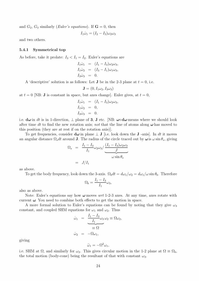
5.4.1 Symmetrical top

As before, take it prolate: I3 < I1 = I2. Euler’s equations are

I1ω1 = (I1 − I3)ω2ω3,

I1ω2 = (I3 − I1)ω1ω3,

I3ω3 = 0.

A ‘descriptive’ solution is as follows: Let J be in the 2-3 plane at t = 0, i.e.

J = (0, I1ω2, I3ω3)

at t = 0 [NB: J is constant in space, but axes change]. Euler gives, at t = 0,

I1ω1 = (I1 − I3)ω2ω3,

I1ω2 = 0,

I3ω3 = 0.

i.e. dω in dt is in 1-direction, ⊥ plane of 3, J etc. [NB: ω+dωmeans where we should lookafter time dt to find the new rotation axis; not that the line of atoms along ω has moved tothis position (they are at rest if on the rotation axis)].

To get frequencies, consider dω in plane ⊥ J [i.e. look down the J -axis]. In dt it movesan angular distance Ωsdt around J. The radius of the circle traced out by ω is ω sin θs, giving

Ωs =I1 − I3I1

ω2ω3/(I1 − I3)ω2ω3

J︸ ︷︷ ︸

ω sin θs

= J/I1

as above.To get the body frequency, look down the 3-axis. Ωbdt = dω1/ω2 = dω1/ω sin θb. Therefore

Ωb =I1 − I3I1

ω3,

also as above.Note: Euler’s equations say how ωmoves wrt 1-2-3 axes. At any time, axes rotate with

current ω. You need to combine both effects to get the motion in space.A more formal solution to Euler’s equations can be found by noting that they give ω3

constant, and coupled SHM equations for ω1 and ω2. Thus

ω1 =I1 − I3I1

ω3

︸ ︷︷ ︸

ω2 ≡ Ωω2,

≡ Ω

ω2 = −Ωω1,

givingω1 = −Ω2ω1,

i.e. SHM at Ω, and similarly for ω2. This gives circular motion in the 1-2 plane at Ω ≡ Ωb,the total motion (body-cone) being the resultant of that with constant ω3.

24

5.4.2 Asymmetrical top

Euler’s equations can be used to derive the behaviour of an asymmetrical top for J near toan axis, say the 3-axis. Put

ω1 = ω10eiΩt, ω2 = ω20e

iΩt, both ω3.

Then Euler’s equations give

Ω2 =(I1 − I3)(I2 − I3)

I1I2ω2

3.

If the I3 above is the largest or the smallest of the three values, Ω2 is positive, implyingoscillatory ω1 and ω2; ω undergoes small stable oscillations about the 3-axis.

If I3 is the middle of the three values, Ω2 is negative, implying exponential behaviour of ω1

and ω2, i.e. rotation about the intermediate axis is unstable.

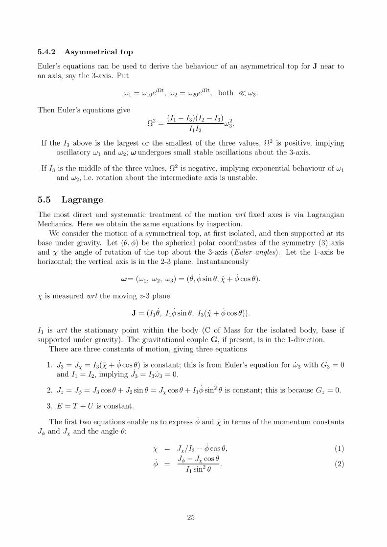
5.5 Lagrange

The most direct and systematic treatment of the motion wrt fixed axes is via LagrangianMechanics. Here we obtain the same equations by inspection.

We consider the motion of a symmetrical top, at first isolated, and then supported at itsbase under gravity. Let (θ, φ) be the spherical polar coordinates of the symmetry (3) axisand χ the angle of rotation of the top about the 3-axis (Euler angles). Let the 1-axis behorizontal; the vertical axis is in the 2-3 plane. Instantaneously

ω= (ω1, ω2, ω3) = (θ, φ sin θ, χ+ φ cos θ).

χ is measured wrt the moving z-3 plane.

J = (I1θ, I1φ sin θ, I3(χ+ φ cos θ)).

I1 is wrt the stationary point within the body (C of Mass for the isolated body, base ifsupported under gravity). The gravitational couple G, if present, is in the 1-direction.

There are three constants of motion, giving three equations

1. J3 = Jχ = I3(χ + φ cos θ) is constant; this is from Euler’s equation for ω3 with G3 = 0and I1 = I2, implying J3 = I3ω3 = 0.

2. Jz = Jφ = J3 cos θ + J2 sin θ = Jχ cos θ + I1φ sin2 θ is constant; this is because Gz = 0.

3. E = T + U is constant.

The first two equations enable us to express φ and χ in terms of the momentum constantsJφ and Jχ and the angle θ:

χ = Jχ/I3 − φ cos θ, (1)

φ =Jφ − Jχ cos θ

I1 sin2 θ. (2)

25

5.5.1 Force-free motion

The body is isolated in free space. Take the J direction as defining ‘vertical’. Then

Jφ = J since total J is along φ-axis.

Jχ = J cos θ.

Therefore

φ =J(1− cos2 θ)

I1 sin2 θ=J

I1= Ωs,

χ =J cos θ

I3− J

I1cos θ = I3ω3

(1

I3− 1

I1

)

=I1 − I3I1

ω3 = Ωb.

The above constitutes a third derivation of the space and body frequencies Ωs and Ωb. [Tomy mind, the relationships between the different treatments are not at all obvious; text bookscan be baffling since few books give more than one treatment].

5.5.2 With external couple

Hereafter we consider the body supported at its base. I1 is about the support, which is at hfrom the C of Mass.

Equations (1) and (2) give φ and χ as known functions of θ. Once θ is known as a functionof time, φ and χ may in principle be found by integration.

θ may be found from the energy equation

E = 12I1(θ

2 + φ2 sin2 θ) + 12I3(χ + φ cos θ)2 +mgh cos θ = constant.

Substitutions from equations (1) and (2) give

E − J2χ

2I3︸ ︷︷ ︸

= 12I1θ

2 +(Jφ − Jχ cos θ)2

2I1 sin2 θ+mgh cos θ

︸ ︷︷ ︸

. (3)

E ′ U ′(θ)

The problem is now solved in principle, since θ is a known function of θ and may be integratedto give θ(t); φ and χ then follow. The integrations involve elliptic integrals and are well beyondthe scope of IB mathematics.

The important physical results can be seen without resource to the full mathematics bytreating the θ motion as oscillation in an effective potential U ′ (cf §4.2.1 for the similartreatment of orbits).

Steady precession arises when θ is at the ‘equilibrium’ position (minimum of U ′) and con-stant; it is physically a special case and requires E ′ = U ′

min. Equations (1) and (2)

then show that φ and χ are constant. The motion thus consists of steady rotation byχ about the symmetry axis, with the axis itself steadily precessing by φ at constant θto the vertical.

If E ′ is slightly larger than the minimum of U ′, then the θ motion can be treated as approx-imate SHM by Taylor expansion of U ′ about the minimum. The oscillations of θ givenutation, i.e. oscillations in χ and φ about the steady precession values.

26

5.5.3 Precession

The condition for steady precession is dU ′/dθ = 0, which gives an equation for θ in terms ofthe constants Jφ and Jχ. After some algebra, it may be rewritten (using equation (2)) as

φ2I1 cos θ − φJχ +mgh = 0. (4)

Equation (4) is useful since it gives us the steady precession speed φ as a function of inclinationθ. It is a quadratic, with solutions

φ =Jχ ±

√

J2χ − 4I1mgh cos θ

2I1 cos θ.

These shows that if cos θ is positive (i.e. the top is standing above its base and not hangingbelow it), φ is impossible unless

J2χ ≥ 4I1mgh cos θ.

Thus steady precession requires the top to be spinning fast enough. In the ‘gyroscopic limit’(very large J from rapid rotation about the symmetry axis) J 2

χ mghI1 and the inequalityis enormously oversatisfied.

The quadratic for φ shows there are two possible precession frequencies for given θ; in thegyroscopic limit they are

φ ≈ mgh/Jχ, independent of θ; this is the ‘slow precession’, as derived in IA.

φ ≈ Jχ/I1 cos θ, independent of G; this is the ‘free precession’ as derived above by Poinsotor Euler; J is entirely in the z-direction and φ ≡ Ωs.

5.5.4 Nutation

The analysis of nutation about precession at general θ, even in the gyroscopic limit, is alge-braically laborious. The case of nutation of a horizontal gyroscope is reasonably straightfor-ward.

Ex. 6 Nutation of a gyroscope, with axis horizontal and supported at one end.

θ0 = 90. Put θ = π/2 + ε. For small ε, cos θ ≈ −ε, sin θ ≈ 1− ε2/2. Then

U ′(θ) = constant + ε(JφJχI1−mgh

)

+ ε2(

J2χ

2I1+J2φ

2I1

)

+ · · ·

for power series expansion in ε. The term ∝ ε is zero at θ0; therefore

Jφ =mghI1Jχ

; φ =mgh

Jχ.

The gyroscope condition is J2χ mghI1 and hence J2

φ. The ε2-term gives the ‘restoringforce’ term in U ′ and hence the equation of motion as follows

U ′ = constant + ε2J2χ

2I1,

I1ε+J2χ

I1ε = 0.

27

This gives SHM in ε at Ω ≡ Ωs = Jχ/I1.It is instructive, and relatively easy, to derive this simple result from first principles.Another limiting case that can be handled relatively easily is the conical pendulum, i.e. as

above but with I3 = 0. There is no gyroscopic action and the pendulum can only hang belowthe support (for motion at steady θ). Note that cf conventional treatments, θ is measuredfrom the upward rather than downward vertical.

28

6 Normal modes

The dynamics of n-parameter systems, or ‘coupled systems’, e.g.:

A molecule of N atoms, treated as N point-nuclei; n = 3N

Two LRC circuits with mutual inductance; n = 2

Waves on strings, in solids etc; n very large, e.g. 1020+

We deal first with the basic theory for N similar masses, taking as a worked example twomasses in 1D motion.

6.1 Basic theory

6.1.1 Equations of Motion

mxi = Fi; i = 1, n

i ≡ one cartesian component of one particle; or

mx = F

in nD space.Suppose system is elastic, i.e. there is a potential energy U ≡ U(x1, . . . xn)

Fi = −∂U∂xi

.

Equilibrium position ≡ minimum of U . We study oscillations about Umin. Take origin in nDspace at minimum of U . Taylor expansion gives

U(x) = U0 +∑

j

(

∂U

∂xj

)

0︸ ︷︷ ︸

xj +∑

j

∑

k

12

(

∂2U

∂xj∂xk

)

0︸ ︷︷ ︸

xjxk + · · ·

= 0 ≡ bjk

The U0 term is irrelevant (the arbitrary zero of PE); the next term is zero, since ∂U/∂xj = 0at the minimum of U . The really important term is the quadratic term. Note that bkj = bjk.

U(x) =∑

j

∑

k

12bjkxjxk = 1

2x′bx;

in the matrix notation, x′ is the transpose of the nD column matrix x. The force Fi comesfrom the derivative −∂U/∂xi of this quadratic form and is (see § 1.3.5 if not immediatelyobvious)

Fi = −∂U∂xi

= −∑

j

bijxj; or F = −gradU = −bx.

The equations of motion are thusmx = −bx.

In simple cases, the equations would often be written down directly, rather than obtainedfrom the expression for U .

29

Ex. 7 Two equal masses m at l and 2l from end of a light spring of total length 3l stretchedbetween fixed supports; consider just motion parallel to length of spring.

Measure x1, x2 from equilibrium position. Equations of motion are

mx1 = −kx1 + k(x2 − x1)

mx2 = −k(x2 − x1)− kx2

where k is the force constant for each third of the spring. Or

m

(

x1

x2

)

= − k(

2 −1−1 2

)

︸ ︷︷ ︸

(

x1

x2

)

≡ b

U = 12k(extension)2 for each spring; i.e.

U = 12kx2

1 + 12k(x1 − x2)

2 + 12kx2

2 = k[

x21 + x2

2 − x1x2

]

or 12

∑

i

∑

j bijxixj as expected.

6.1.2 Oscillations

Def n. 8 Normal mode: An oscillation when all parts of a system oscillate at the same

frequency, i.e. the same eiωt time-variation everywhere.

A normal mode implies a constant amplitude and phase relation between the xi’s, i.e. betweendifferent parts of the system. Put

x = x0eiωt,

x = −ω2x,

mω2x = bx.

Therefore possible mω2’s for normal modes are the eigen values of b; there are n of them.The eigen vectors ej, j = 1, n give the actual modes, i.e. the amplitude and phase relationsbetween different parts of the system [the theory gives only the direction of ej in nD space;the magnitude, = overall amplitude, is indeterminate].

Ex. 7 (contd.)

xi = xi0eiωt; i = 1, 2

−mω2

(

x1

x2

)

= −k(

2 −1−1 2

)(

x1

x2

)

.

To get eigen values, rewrite as

2− mω2

k−1

−1 2− mω2

k

(

x1

x2

)

= 0. (1)

30

For a non-trivial solution for x1, x2, the determinant of the 2 × 2 matrix must be zero.Therefore

(

2− mω2

k

)2

− 1 = 0,

or

ω2 =k

mor

3k

m.

The eigen vectors in this case are

1. ω2 = k/m. Either of the equations in (1) gives x1 − x2 = 0, or x1 = x2, i.e. massesoscillate in phase with equal amplitude.

2. ω2 = 3k/m. Equations (1) give −x1 − x2 = 0, or x1 = −x2, i.e. masses oscillate inantiphase with equal amplitude.

6.1.3 Orthogonality

Matrix b is symmetrical, therefore its eigen vectors are orthogonal in nD space:

ei · ej = 0 if i 6= j.

1. If ωi’s are all different, ei’s are unique.

2. If some ωi’s are the same, then there is a choice of ei’s, but you can always findorthogonal ei’s [if ea and eb are eigen vectors with the same ω, then so is any linearcombination αea + βeb].

The ei’s are the ‘natural axes’ in nD space. With respect to them

U =∑

i

∑

j

12b′ijx

′

ix′

j

with

b′ = m

ω21 . .. ω2

2 .. . ω2

3

,

i.e. b is diagonal. U =∑ 1

2mω2

i x′2i =

∑U for each normal mode separately.

Ex. 7 (contd.)

e1 =

(

11

)

; e2 =

(

1−1

)

.

Take new coordinates wrt eigen-vector axes

xs =1√2(x1 + x2); xd =

1√2(x1 − x2);

or

x1 =1√2(xs + xd); x2 =

1√2(xs − xd).

31

Then

U = k[x21 + x2

2 − x1x2]

= k 12

[

(xs + xd)2 + (xs − xd)2 − (xs + xd)(xs − xd)

]

= k 12(x2

s + 3x2d);

as expected, the cross-terms cancel. The equations of motion are

mxs = −kxs

mxd = −3kxd

i.e. the motions are uncoupled, giving independent oscillations, of xs with mω2 = k, and xdwith mω2 = 3k.

6.1.4 Energy

Kinetic energy = T =∑

i12miv

2i = 1

2m | x |2; x is the velocity vector in nD space. Now

| vector | is independent of choice of orthogonal axes, and so

T = 12m | x′ |2=

∑

T for each mode;

[x′ is wrt eigen-vector axes].

Ex. 7 (contd.)

T = 12m(x2

1 + x22) = 1

2m(x2

s + x2d).

Energy = T + U = 12mx2

s + 12kx2

s︸ ︷︷ ︸

+ 12mx2

d + 32kx2

d︸ ︷︷ ︸

.

xs mode xd mode

mω2s = k mω2

d = 3k

In oscillation

1. T = U for each mode (overline ≡ time-average).

2. E =∑E over modes.

Ex. 8 Two pendulums, weakly coupled; each in 1D motion in parallel planes

Modes of oscillation are

1. In phase with equal amplitude θs

2. In antiphase with equal amplitude θd

32

By inspection these are the normal modes — each oscillates at a single ω, and for a 2-parameter system there can only be 2 modes. ωs, for the first mode, is the same as foruncoupled pendulums; ωd is a little faster.

Suppose initially θ1 (of pendulum 1) = θ0, θ2 = 0 and both are stationary [NB: 4 initialconditions]. At t = 0,

θs = θd =1√2θ0

and at later time

θs =θ0√2eiωst, θd =

θ0√2eiωdt,

giving beats at the difference frequency; when (ωd−ωs)t = π, pendulum 2 has large amplitudeand pendulum 1 is stationary. The system can be viewed as

1. Two oscillators, with weak coupling and periodic interchange of energy between themat the beat frequency; or

2. One 2D system, with 2 modes and no transfer of energy between modes.

6.2 Extensions

6.2.1 Masses different

Ex. 9 CO2 molecule; linear with masses M (carbon) and m (oxygen); 1D motion along lineof nuclei

b = k

1 −1 .−1 2 −1. −1 1

and

m1 . .. m2 .. . m3

︸ ︷︷ ︸

x = −bx (2)

≡ m

for three general masses. If all of system oscillates as eiωt, then mω2x = bx, and the ω’s aregiven by

det(mω2 − b) = 0. (3)

These are not strictly eigen value equations, though they may be easy enough to handle.The usual way of making use of the previous theory is via mass-weighted coordinates.

Introduce ξi = xi√mi. Then

√miξi = −

∑

j

bijξj√mj

.

On dividing by√mi,

ξi = −∑

j

bij√mimj

︸ ︷︷ ︸

ξj.

symmetrical; eigen values give ω2

33

We have scaled our original x1-x2-x3 space parallel to the 1-2-3 axes so that the same | ξi |≡same kinetic energy. Eigen vectors become orthogonal and the theory of § 6.1 applies.

Ex. 9 (contd.)

The modes for CO2 are

1. ω2 = 0, e1 = (1, 1, 1), i.e. translational motion of molecule as a whole.

2. ω2 = k/m, e2 = (1, 0,−1), i.e. carbon stationary, oxygens in antiphase.

3. ω2 = k(2m+M)/Mm, e3 = (1,−2m/M, 1), i.e. oxygens in phase with each other andin antiphase with carbon; no motion of C of Mass.

The modes could probably have been guessed by inspection.

6.2.2 Extended masses

N-parameter systems involving rigid bodies will often have equations of motion similar tothose of (2) but with the LHS matrix m non-diagonal; the coordinates represented by thevector x will often be angular instead of linear, or a mix of both. These can be transformedinto the simpler type used in § 6.1 by suitable change of coordinates (see Riley). Simple casesare best treated by handling the equivalent equation (3) directly.

6.3 Many parameter systems

Ex. 10 Standing waves on a string, tension F , mass ρ per unit length; total length l, anchoredon x-axis at x = 0, x = l; motion in xy-plane. Assume small angle deviations, i.e. F cos θ ≈ Feverywhere.

6.3.1 Equations of motion

Motion of an element dx is

ρdxy = F (θ2 − θ1) = F∂θ

∂xdx.

θ ≈ ∂y/∂x, therefore

ρy = F∂2y

∂x2,

the non-dispersive wave equation.

6.3.2 Normal modes

Normal modes imply a solution of the form y = y(x)eiωt, so

−ω2ρy(x) = F∂2y

∂x2,

which is the SHM equation, with solution

y(x) = Ak cos(kx + φk)

in which

34

Ak and φk are arbitrary constants,

ω2ρ = Fk2 — the dispersion relation, and

v = velocity of wave = ω/k =√

F/ρ, and is independent of ω, k.

For a string of length l, the boundary conditions that y = 0 at x = 0 and x = l give

y(x) = Bk sin(kx)

with no cos term, and kl = nπ. Put k = nk0, ω = nω0, where k0 and ω0 are the values for

the lowest mode, k0 = π/l, ω0 = π

l

√

F/ρ. The general y(x, t) is then

y =∑yn =

∞∑

n=1

sin(nk0x) [Cn cos(nω0t) + Sn sin(nω0t)]︸ ︷︷ ︸

.

≡ tn(t)

y can be thought of as a vector in∞D space, one dimension for each value of x. Each n of theabove is one normal mode, with Cn and Sn the amplitudes of the in-phase and quadraturecomponents. yn = sin(nk0x) is the nth eigen function, equivalent to an eigen vector in ∞Dspace.

6.3.3 Energy

The orthogonality relations between the eigen vectors/functions are

yn · ym =∫ l

0sin(nk0x) sin(mk0x)dx = 0,

and similarly∫ l

0cos(nk0x) cos(mk0x)dx = 0,

for n 6= m.U =

∫ l0 F (ds − dx), where dx is the original length of an element of string and ds the

length it is stretched to by the wave. Simple geometry gives

U =∫ l

0

12F

(

∂y

∂x

)2

dx;

∂y

∂x=∑

n

nk0 cos(nk0x)tn(t).

The expression for U is of the form∫

(∑

term)2. But by orthogonality the cross-terms in(∑

term)2 go to zero on integration. We are thus just left with∫ ∑

(term2). The result is

U = 14F l∑

n2k20t

2n

using the fact that < cos2 >= 12

in x-integration. The time-average of U is

U = 18F lk2

0

∑

n2(C2n + S2

n)

using < t2n >= 12(C2

n + S2n). Note that U =

∑

n Un.

35

The kinetic energy is

T =∫

12ρ

(

∂y

∂t

)2

dx

and after similar evaluations gives

T = 18ρlω2

0

∑

n2(C2n + S2

n).

As Fk20 = ρω2

0, U = T . Also E = T + U is constant for each mode; thus for the Cn-term,

E = 14F lk2

0n2C2

n

[

cos2(nω0t)︸ ︷︷ ︸

+ sin2(nω0t)︸ ︷︷ ︸

]

.

U-part T-part

36

7 Elasticity — Fundamentals

Hooke’s law: ‘Ut tensio, sic vis’ (his words).

7.1 Basic ideas

Ex. 11 A wire of length l, width w, uniform cross-sectional area A. Force F stretches it tolength l + δl.

Def n. 9 Stress: τ (or σ, S, . . . ) ≡ F/A.

Def n. 10 Strain: e (or u, . . . ) ≡ δl/l.

Def n. 11 Young’s modulus: E (or Y , . . . ) ≡ stress/strain.

Note

1. F is the force across any transverse cut; it is the same for all cuts since the piece ofwire between any two cuts is in equilibrium.

2. Stress and strain are local as well as global properties. Young’s modulus is independentof dimensions and is a property of the material.

3. Young’s Modulus is stress/strain defined for this specific geometry.

The width can also change, by δw.

Def n. 12 Poisson’s ratio: σ (or ν, . . . ) ≡ −(δw/w)/(δl/l).

As with Young’s modulus, Poisson’s ratio is defined for this specific geometry.We need to generalise to full 3D geometry (and in principle anisotropic media).

7.2 Stress

Force and area are really vectors F and A. They need not be parallel.

Ex. 12 Take Ex. 11 and take an oblique cut. A is perpendicular to the cut and of magnitudeA0 sec θ (A0 is the ordinary transverse area). F is still the same, parallel to the length. Withaxes, x parallel to the length, y and z transverse,

Fx = τAx; Fy = Fz = 0

i.e. a matrix or tensor relationship between vectors F and A.

We can see that the relation between F and A must in general be a matrix as follows.Consider a polyhedron-shaped element in a material in equilibrium under uniform stress. F

on polyhedron = 0 =∑

a Fa exerted over its faces. Also A =∑

a Aa over faces = 0 for aclosed polyhedron (? IA result; if not prove simply by summing each Cartesian component =projected area). This is true for any polyhedron = any set of Aa, and implies that Fa mustbe linear with, i.e. proportional to, Aa though not necessarily parallel to it; or

Fi =∑

j

τijAj.

37

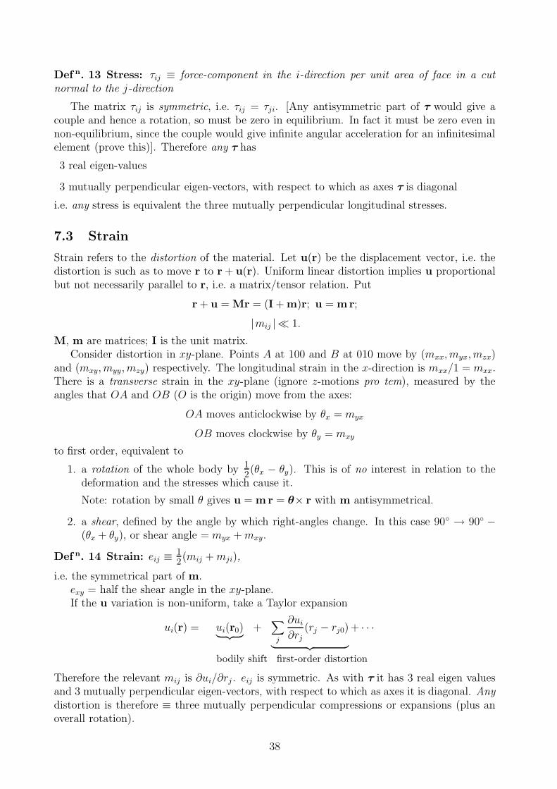
Def n. 13 Stress: τij ≡ force-component in the i-direction per unit area of face in a cutnormal to the j-direction

The matrix τij is symmetric, i.e. τij = τji. [Any antisymmetric part of τ would give acouple and hence a rotation, so must be zero in equilibrium. In fact it must be zero even innon-equilibrium, since the couple would give infinite angular acceleration for an infinitesimalelement (prove this)]. Therefore any τ has

3 real eigen-values

3 mutually perpendicular eigen-vectors, with respect to which as axes τ is diagonal

i.e. any stress is equivalent the three mutually perpendicular longitudinal stresses.

7.3 Strain

Strain refers to the distortion of the material. Let u(r) be the displacement vector, i.e. thedistortion is such as to move r to r + u(r). Uniform linear distortion implies u proportionalbut not necessarily parallel to r, i.e. a matrix/tensor relation. Put

r + u = Mr = (I + m)r; u = mr;

|mij | 1.

M, m are matrices; I is the unit matrix.Consider distortion in xy-plane. Points A at 100 and B at 010 move by (mxx, myx, mzx)

and (mxy, myy, mzy) respectively. The longitudinal strain in the x-direction is mxx/1 = mxx.There is a transverse strain in the xy-plane (ignore z-motions pro tem), measured by theangles that OA and OB (O is the origin) move from the axes:

OA moves anticlockwise by θx = myx

OB moves clockwise by θy = mxy

to first order, equivalent to

1. a rotation of the whole body by 12(θx − θy). This is of no interest in relation to the

deformation and the stresses which cause it.

Note: rotation by small θ gives u = mr = θ× r with m antisymmetrical.

2. a shear, defined by the angle by which right-angles change. In this case 90 → 90 −(θx + θy), or shear angle = myx +mxy.

Def n. 14 Strain: eij ≡ 12(mij +mji),

i.e. the symmetrical part of m.exy = half the shear angle in the xy-plane.If the u variation is non-uniform, take a Taylor expansion

ui(r) = ui(r0)︸ ︷︷ ︸

+∑

j

∂ui∂rj

(rj − rj0)︸ ︷︷ ︸

+ · · ·

bodily shift first-order distortion

Therefore the relevant mij is ∂ui/∂rj . eij is symmetric. As with τ it has 3 real eigen valuesand 3 mutually perpendicular eigen-vectors, with respect to which as axes it is diagonal. Anydistortion is therefore ≡ three mutually perpendicular compressions or expansions (plus anoverall rotation).

38

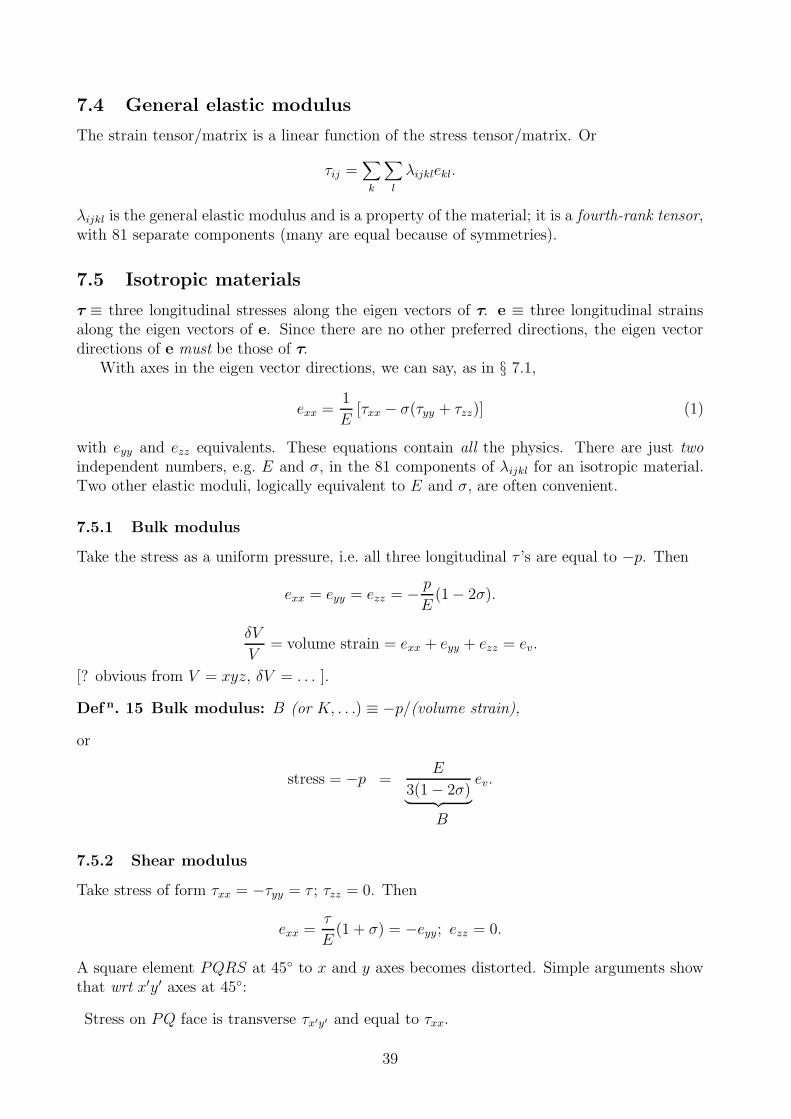
7.4 General elastic modulus

The strain tensor/matrix is a linear function of the stress tensor/matrix. Or

τij =∑

k

∑

l

λijklekl.

λijkl is the general elastic modulus and is a property of the material; it is a fourth-rank tensor,with 81 separate components (many are equal because of symmetries).

7.5 Isotropic materials

τ ≡ three longitudinal stresses along the eigen vectors of τ. e ≡ three longitudinal strainsalong the eigen vectors of e. Since there are no other preferred directions, the eigen vectordirections of e must be those of τ.

With axes in the eigen vector directions, we can say, as in § 7.1,

exx =1

E[τxx − σ(τyy + τzz)] (1)

with eyy and ezz equivalents. These equations contain all the physics. There are just twoindependent numbers, e.g. E and σ, in the 81 components of λijkl for an isotropic material.Two other elastic moduli, logically equivalent to E and σ, are often convenient.

7.5.1 Bulk modulus

Take the stress as a uniform pressure, i.e. all three longitudinal τ ’s are equal to −p. Then

exx = eyy = ezz = − pE

(1− 2σ).

δV

V= volume strain = exx + eyy + ezz = ev.

[? obvious from V = xyz, δV = . . . ].

Def n. 15 Bulk modulus: B (or K, . . .) ≡ −p/(volume strain),

or

stress = −p =E

3(1− 2σ)︸ ︷︷ ︸

ev.

B

7.5.2 Shear modulus

Take stress of form τxx = −τyy = τ ; τzz = 0. Then

exx =τ

E(1 + σ) = −eyy; ezz = 0.

A square element PQRS at 45 to x and y axes becomes distorted. Simple arguments showthat wrt x′y′ axes at 45:

Stress on PQ face is transverse τx′y′ and equal to τxx.

39

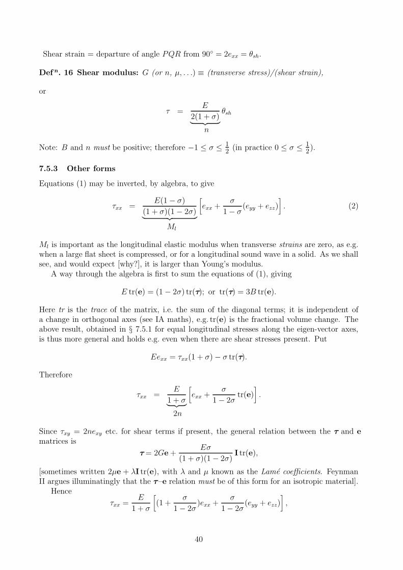
Shear strain = departure of angle PQR from 90 = 2exx = θsh.

Def n. 16 Shear modulus: G (or n, µ, . . .) ≡ (transverse stress)/(shear strain),

or

τ =E

2(1 + σ)︸ ︷︷ ︸

θsh

n

Note: B and n must be positive; therefore −1 ≤ σ ≤ 12

(in practice 0 ≤ σ ≤ 12).

7.5.3 Other forms

Equations (1) may be inverted, by algebra, to give

τxx =E(1− σ)

(1 + σ)(1− 2σ)︸ ︷︷ ︸

[

exx +σ

1− σ (eyy + ezz)]

. (2)

Ml

Ml is important as the longitudinal elastic modulus when transverse strains are zero, as e.g.when a large flat sheet is compressed, or for a longitudinal sound wave in a solid. As we shallsee, and would expect [why?], it is larger than Young’s modulus.

A way through the algebra is first to sum the equations of (1), giving

E tr(e) = (1− 2σ) tr(τ); or tr(τ) = 3B tr(e).

Here tr is the trace of the matrix, i.e. the sum of the diagonal terms; it is independent ofa change in orthogonal axes (see IA maths), e.g. tr(e) is the fractional volume change. Theabove result, obtained in § 7.5.1 for equal longitudinal stresses along the eigen-vector axes,is thus more general and holds e.g. even when there are shear stresses present. Put

Eexx = τxx(1 + σ)− σ tr(τ).

Therefore

τxx =E

1 + σ︸ ︷︷ ︸

[

exx +σ

1− 2σtr(e)

]

.

2n

Since τxy = 2nexy etc. for shear terms if present, the general relation between the τ and e

matrices is

τ= 2Ge +Eσ

(1 + σ)(1− 2σ)I tr(e),

[sometimes written 2µe + λI tr(e), with λ and µ known as the Lame coefficients. FeynmanII argues illuminatingly that the τ–e relation must be of this form for an isotropic material].

Hence

τxx =E

1 + σ

[

(1 +σ

1− 2σ)exx +

σ

1− 2σ(eyy + ezz)

]

,

40

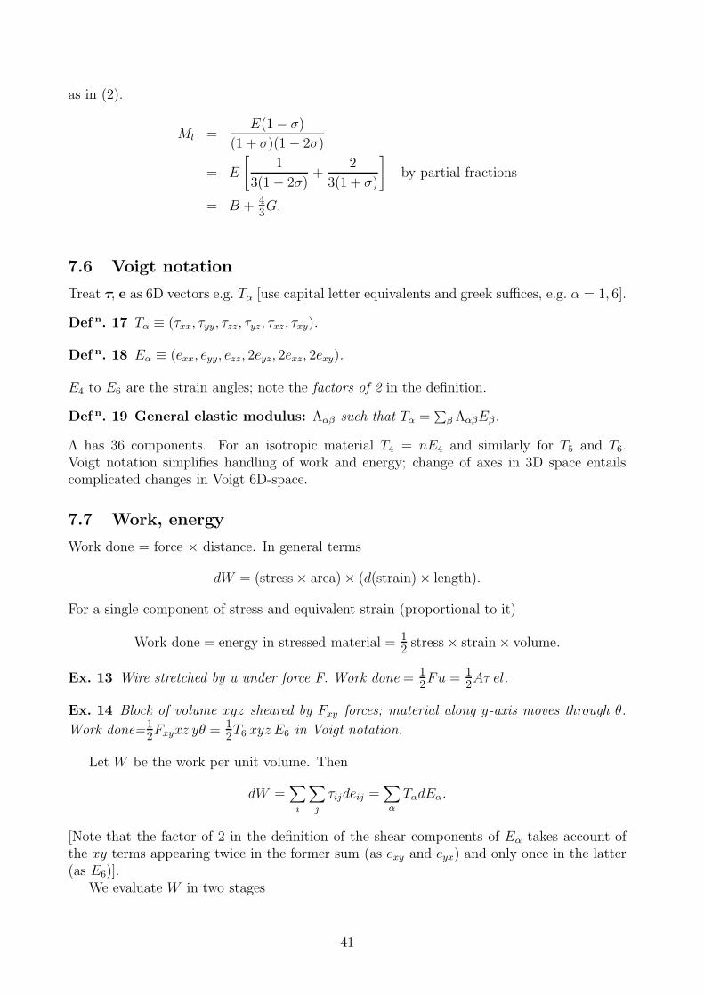
as in (2).

Ml =E(1− σ)

(1 + σ)(1− 2σ)

= E

[

1

3(1− 2σ)+

2

3(1 + σ)

]

by partial fractions

= B + 43G.

7.6 Voigt notation

Treat τ, e as 6D vectors e.g. Tα [use capital letter equivalents and greek suffices, e.g. α = 1, 6].

Def n. 17 Tα ≡ (τxx, τyy, τzz, τyz, τxz, τxy).

Def n. 18 Eα ≡ (exx, eyy, ezz, 2eyz, 2exz, 2exy).

E4 to E6 are the strain angles; note the factors of 2 in the definition.

Def n. 19 General elastic modulus: Λαβ such that Tα =∑

β ΛαβEβ.

Λ has 36 components. For an isotropic material T4 = nE4 and similarly for T5 and T6.Voigt notation simplifies handling of work and energy; change of axes in 3D space entailscomplicated changes in Voigt 6D-space.

7.7 Work, energy

Work done = force × distance. In general terms

dW = (stress× area)× (d(strain)× length).

For a single component of stress and equivalent strain (proportional to it)

Work done = energy in stressed material = 12

stress× strain× volume.

Ex. 13 Wire stretched by u under force F. Work done = 12Fu = 1

2Aτ el.

Ex. 14 Block of volume xyz sheared by Fxy forces; material along y-axis moves through θ.

Work done=12Fxyxz yθ = 1

2T6 xyz E6 in Voigt notation.

Let W be the work per unit volume. Then

dW =∑

i

∑

j

τijdeij =∑

α

TαdEα.

[Note that the factor of 2 in the definition of the shear components of Eα takes account ofthe xy terms appearing twice in the former sum (as exy and eyx) and only once in the latter(as E6)].

We evaluate W in two stages

41

7.7.1 dW is a ‘perfect differential’

i.e.∫ B

AdW = WB −WA

is independent of the path between in initial (A) and final (B) configurations of Tα and Eα.This is because the deformations are elastic and energy is conserved. Standard maths thengives

∂2W

∂Eα∂Eβ=

∂2W

∂Eβ∂Eα,

or∂Tα∂Eβ

=∂Tβ∂Eα

,

or Λαβ = Λβα, giving at most 21 independent components (the most general type of anisotopicmaterials have this many elastic constants).

7.7.2 Integration of W

Let the initial Eα’s all be zero (unstressed) and grow proportionately to the final state (i.e.steady growth in the same direction in 6D Voigt-space); this is a specific path of integration,but we have just shown that all paths give the same answer.

dW =∑

α

TαdEα =∑

α

(∑

β

ΛαβEβ)dEα,

orW =

∑

α

∑

β

12ΛαβEαEβ,

since each of the 36 terms summed is of the form∫ 10 fEβ dfEα, where f is the fraction of the

final value. The non-Voigt form is

W =∑

i

∑

j

∑

k

∑

l

12λijkleijekl.

42

8 Elasticity — Applications

8.1 Simple examples

Ex. 15 Long thin cylindrical tube, wall thickness t radius r; pressure p inside.

Take cylindrical coordinates; in these coordinates all stresses and strains are longitudinal(tensors diagonal). The circumferential stress τφφ is obtainable from the equilibrium of halfthe cylinder sliced lengthways. Force on half of cylinder gives

2tτφφ = 2rp; or τφφ = pr

t.

The lengthways stress τzz is got from the force on the closed ends:

2πrtτzz = πr2p; or τzz = pr

2t.

The radial stress τρρ will depend on the depth within the wall, but will be of the order of pand so tiny cf τφφ and τzz. Therefore the circumferential change eφφ is

eφφ =1

E(τφφ − στzz) =

pr

Et

(

1− 12σ)

.

ezz is found analogously.

Ex. 16 Torsion of a solid cylindrical wire, twisted through an angle φ in length l.

Consider annular element of radius r and thickness t r. θ = shear angle = rφ/l. Thereforeforce per unit area at a cross-section is nθ. Couple, of all forces acting at a cross-section ofthe annular element, is

C = r Gθ 2πrt =2πr3tG

lφ.

For a solid wire, put t equal to dr and integrate:

C =πr4G

2lφ.

8.2 Bending of beams

Consider a thin beam bent into an arc of radius R (which may vary down the beam). Theinner side of the beam will be compressed, the outer expanded. A sheet in the middle, theneutral axis, will retain its original length.

Def n. 20 Bending moment: couple produced by stress forces at a transverse cut acrossthe beam.

For an isolated beam in equilibrium, the bending moment must be the same all along thebeam and equal to the external couples applied at its ends.

Measure ξ across the beam from the neutral axis. A strand of material at ξ of originallength Rθ will be stretched to (R + ξ)θ by the bending. Therefore

strain = dl/l = ξ/R

43

or the bending moment, obtained by integrating across the area,

B =∫

Eξ

RdA

︸ ︷︷ ︸

ξ =E

R

∫

ξ2dA.

force on dA∫

ξ2dA is the ‘moment of area’ about the neutral axis, and is a measure of the stiffness, whichtherefore goes as (linear size)4.

Ex. 17 Light rod, length l, clamped horizontally at one end, weight W at the other. Assumesmall angular deviations.

Take x along rod, y(x) = downwards displacement. For a rectangular cross-section a highand b wide, and the neutral axis in the middle,

I =∫

ξ2dA =a3b

12.

Consider equilibrium from x to the end. Total B on this piece of beam = 0. The bendingmoment B at x is therefore given by

B = W (l − x).

For this geometry y′′ = 1/R, soEIy′′ = W (l − x);

EIy′ = W

(

lx− x2

2+ C1

)

; C1 = 0, since y′ = 0 at x = 0.

EIy = W

(

lx2

2− x3

6+ C0

)

; C0 = 0, since y = 0 at x = 0.

Ex. 18 The same rod, but bending under its own weight.

Let w(x)dx be the weight of length dx; no W at end. Let F (x) be the vertical force exertedacross any transverse section (like y, measure it downwards).

Consider equilibrium of dx. Stress forces are F down (at x) and F + dF up (at x+ dx).Therefore

dF = w(x)dx; dF/dx = w(x).

Consider now the couple. The vertical stress forces produce a couple Fdx. This must justbalance the difference in the bending moments at the two ends of dx, i.e.

dB = Fdx; dB/dx = F (x).

Therefore

EIy′′ = B(x),

EIy′′′ = F (x),

EIy′′′′ = w(x).

If w is uniform, and equal to say W/l, then

EIy′′′ =∫

wdx =W

lx+ C3 = W

(x

l− 1

)

44

using F = 0 at x = l.

EIy′′ = W

(

x2

2l− x + C2

)

= W

(

x2

2l− x +

l

2

)

using B = 0 at x = l.y′(x) and y(x) follow from further integrations, with y′ = y = 0 at x = 0.

8.3 Euler strut

A rod of length l is subject to a compressional force F parallel to its length. Imagine Fincreasing slowly. For small F the rod is compressed but stays straight. When F exceeds acertain value, the rod ‘bows’ and departs markedly from being straight. The onset of bowingis sudden; why, and at what force?

8.3.1 Equilibrium analysis

If the rod is ‘bowed’, the moment of the end force F at a point on the rod displaced to y isFy. This must balance the bending moment if in equilibrium, giving (with due regard forsigns)

EIy′′ + Fy = 0

i.e. an SHM equation for y(x) with solution

y = y0 sin

√

F

EIx

(y = 0 at x = 0, so the cos term can be omitted). The wavelength λ = 2π√

EIF

; there will be

a physically possible solution other than y = 0 if λ/2 fits into l. In detail

y = y0 sin

√

F

EIx and must be zero at x = l.

1. If√

FEI

< π, y0 = 0 is the only possibility. The rod does not bow.

2. If√

FEI

= π, y = 0 whatever y0, i.e. bowing is equally possible at any amplitude. Therod is in neutral equilibrium as between different values of y0.

3. If√

FEI

> π, y0 = 0 is an unstable solution. The easiest way of seeing this is via energy.

8.3.2 Energy

Take rod of form y = y0 sin kx; kl = π. We evaluate

(a) Energy stored in bent beam. Energy =∫

Bdθ = 12Bθ for each piece (B ∝ θ). Put

θ = dx/R = y′′dx for each length dx and B = EIy′′; integrate over x

W1 =∫

12EI(y′′)2dx = 1

4EIy2

0k4l.

45

(b) Work done by forces at ends as the ends move in towards one another. W2 = F×(arcminus chord).

ds = dx√

1 + y′2 ≈ dx(1 + 12y′2)

givingW2 = 1

4Fy2

0k2l.

The important result is that

W1

W2

=EIk2

Findependent of y0.

We can draw up a table showing which of W1 and W2 is the larger for each of the threesituations listed above

Case: 1 2 3Larger: W1 W1 = W2 W2

y = 0 equilibrium: stable neutral unstable

When the force is sufficient to produce bowing, y0 increases until the small-angle approx-imations in the above treatment cease to be valid; the rod takes an equilibrium positiondetermined by the fuller (and more complicated) equations.

46

9 Elastic waves

9.1 Basic theory

We apply the results of previous sections to the non-equilibrium situation. We have thefollowing chain of relationships, each of whose links we need to think about

u(r) ←→ eij ←→ τij ←→ F ←→ u

displacement strain stress on dV

Wave motion can occur when the stress forces generated by a pattern of displacementsu(r) are sufficient to maintain the pattern.

9.1.1 F and u

We suppose (a) isotropic and homogeneous materials, and (b) strains small ( 1), implyinga constant density and thefore allowing us to write

F on dV = ρdV u

with ρ constant.

9.1.2 τ and F

We need the force on element dV = dxdydz resulting from the stress forces on all its faces.The x-component of the force on the x-facing faces is −τxxdydz on the face at x and +[τxx +(∂τxx/∂x)dx]dydz on the face at x + dx, giving a net contribution to Fx of (∂τxx/∂x)dV .The y-facing and z-facing faces give contributions to Fx of (∂τxy/∂y)dV and (∂τxz/∂z)dVsimilarly, giving a total Fx per unit volume of

Fx/dV =∂τxx∂x

+∂τxy∂y

+∂τxz∂z

.

[More elegant derivation: The i-th component of force on area dA can be written as thescalar product τ i ·dA, where τ i is the vector in the i-th row of the matrix τ. Fi on a volumeis then given by

Fi =∫

τ i · dA =∫

div τ i dV

using the divergence theorem. This is equivalent to an Fi of div τ i per unit volume — thesame result as above.]

9.1.3 τ , e and u

We have

eij = 12

(

∂ui∂xj

+∂uj∂xi

)

and also the results of § 7.5 relating e and τ. We postpone discussion of the general u(r)relationship in favour of dealing first with the two important simple cases (which in factrepresent all the physics).

47

9.2 Plane waves

We shall suppose the waves are travelling the x-direction, i.e. put ∂/∂y = ∂/∂z = 0.

9.2.1 Transverse waves

or ‘Shear waves’ (‘S waves’). We suppose u is in the y-direction, i.e.

u = (0, uy, 0); uy = uy(x, t).

The y-component of force is

Fy/dV =∂τyx∂x

and

τyx = G 2eyx = G

(

∂ux∂y

+∂uy∂x

)

= G∂uy∂x

.

Therefore

ρuy =∂

∂x

(

G∂uy∂x

)

= G∂2uy∂x2

.

This is the non-dispersive wave equation for waves travelling with velocity

vt =√

G/ρ =√

Mt/ρ.

Mt is here used to denote the modulus for transverse waves (it is equal to G).

9.2.2 Longitudinal waves

or ‘Pressure waves’ (‘P waves’). Here we suppose u is in the x-direction, i.e.

u = (ux, 0, 0); ux = ux(x, t).

The relevant force is

Fx/dV =∂τxx∂x

.

With a longitudinal wave, there is no y or z motion and hence eyy = ezz = 0. The τ–erelationship is thus simply τxx = Mlexx (see equation (2) of § 7.5). Therefore

ρux =∂τxx∂x

=∂

∂x(Mlexx) = Ml

∂2ux∂x2

.

This is the non-dispersive wave equation for waves of velocity

vl =√

Ml/ρ.

9.2.3 Relative velocities

As already noted Ml = B+ 43nG. So Ml > Mt; longitudinal waves are faster than transverse.

The ratio(vlvt

)2

=Ml

Mt=B + 4G/3

n=B

G+

43 =

2− 2σ

1− 2σ

where the final expression has been obtained by putting B and G in terms of E and σ (Ecancels and the velocity ratio depends only on σ).

48

9.2.4 Fluids

The characteristic property is that a shear stress cannot be maintained; shear strain exy can

exist without any τxy. Formally one can put G = 0, E = 0, σ = 12. B is the one elastic

constant. The consequences for wave motion are

1. Longitudinal waves: Ml = B, vl =√

B/ρ.

2. Transverse waves: Mt = 0, vt = 0. Physically this implies infinite wavelength, oruniform steady uy with no restoring force.

Note that for longitudinal waves in a solid, the modulus Ml is more than just B; there is ashear as well.

9.2.5 General u(r)

We can write, using the results of § 7.5 and the notation of § 9.1.2

ρux = div (τx) = 2Gdiv (ex) + λdiv (Ix tr(e)).

Ix tr(e) is the vector in the top row of the matrix I tr(e) and is ( tr(e), 0, 0); div of it is

div (Ix tr(e)) =∂

∂xtr(e) =

∂

∂x(exx + eyy + ezz)

=∂

∂x

(

∂ux∂x

+∂uy∂y

+∂uz∂z

)

=∂

∂xdivu.

We also need

2 div (ex) = 2∂

∂x

(

∂ux∂x

)

+∂

∂y

(

∂ux∂y

+∂uy∂x

)

+∂

∂z

(

∂ux∂z

+∂uz∂x

)

= ∇2ux +∂

∂xdiv (u).

Therefore

ρux = G∇2ux + (G+ λ)∂

∂xdivu

orρu = G∇2u + (G+ λ) grad divu.

This equation is in terms of the Lame coefficient

λ =Eσ

(1 + σ)(1− 2σ)= B − 2

3G;

G+ λ = B +G3 .

Transverse waves arise when divu = 0 (no volume change; the planes of material slidesideways). Longitudinal or irrotational waves arise when curlu = 0.

49

9.3 Waves on a plate

Take the plate as in the xy-plane; suppose the thickness λ. The boundary condition isthat there is no force at the surface; τxz = τyz = τzz = 0. The arguments are similar tothose for 3D but with a different τ–e–u relationship. The results, for waves travelling in thex-direction, are

1. u in y-direction: transverse waves with vt =√

G/ρ as in the 3D case.

2. u in x-direction: longitudinal waves with relevant modulus Ml′ = E/(1− σ2). Unlike

the 3D case, ezz is non-zero; the wave produces variations of thickness of the plate.

3. u in z-direction: bending of the plate — see transverse waves on rods below.

9.4 Waves on rods

9.4.1 Torsional waves

Cylindrical rod. From § 8.1, the couple C across surface at x is given by

G =πr4G

2

∂φ

∂x.

The net C on a disc of rod of length dx is

dG =∂G

∂xdx =

πr4G

2

∂2φ

∂x2dx

which is equal todI φ = 1

2ρπr2dx r2 φ

giving the non-dispersive wave equation

ρφ = G∂2φ

∂x2

and velocity v =√

G/ρ.

9.4.2 Transverse waves

The theory of bending beams (see § 8.2) gives

EI∂4y

∂x4= w(x)

where w(x)dx is the external sideways force on dx that would produce equilibrium with thebeam bent to y(x). The equation of motion for non-equilibrium y(x) and no external w istherefore

EIy′′′′ = −ρywhere ρ is the mass per unit length along the rod. For a wave solution of the form y =y0e

i(ωt−kx),EIk4 = ρω2.

The waves are dispersive and this is the dispersion relation; v = ω/k depends on ω.

50

For SHM time-variation y = y(x)eiωt, the space-variation is given by

y′′′′ = k4y; (k as above).

This is a fourth-order differential equation. The general solution has 4 arbitrary constants;one possible form of it is

y = A cos kx +B sin kx+ C cosh kx +D sinh kx,

the values of A,B,C and D being determined by four boundary conditions.

Ex. 19 Free rod of length 2l. What are the frequencies of the symmetrical modes of oscilla-tion?

At the ends, the force F and bending moment G across an interface are both zero. Soy′′′ = y′′ = 0 (see § 8.2) at x = ±l. For symmetrical modes B = D = 0, and substitution ofthe x = ±l conditions gives

G = 0 : 0 = −Ak2 cos kl + Ck2 cosh kl

F = 0 : 0 = +Ak3 sin kl + Ck3 sinh kl

or (for non-zero A and C)tan kl = − tanh kl.

Sketches of tan kl and − tanh kl give solutions at kl = 0 and then slightly greater than 3π

4,

7π

4etc.

9.5 Propagation, impedance

Reminder of standard IA results. Consider longitudinal waves in 3D case.

ux = u0ei(ωt−kx); ux = iωux.

Also

exx =∂ux∂x

= −ikux;

τxx = Mlexx = −ikMlux

so that τxx ∝ ux.

Def n. 21 Impedance: Z ≡ ‘force’/(‘response velocity’), force and response being such thatrate of energy transfer = force × response velocity.

In this case, ‘force’ = τxx and response velocity = ux. Therefore

Z = | τxxux|= kMl

ω=Ml

vl=√

Mlρ.

Rate of work/m2 = |τxxux |=τ 2xx

Z= u2

xZ.

Energy: U = 12

stress × strain per unit volume = 12Mle

2xx per unit volume. T = 1

2ρu2

x perunit volume. As can easily be shown

51

1. U = T .

2. E = T + U = 12Mlk

2u20.

3. E × velocity = energy flow rate.

Ex. 20 Torsional waves on cylindrical rod.

φ(x, t) = φ0ei(ωt−kx). The response velocity is φ = iωφ and the ‘force’ is C. The impedance

is therefore Z = πr4Gk/2ω.

9.6 Reflection of waves — Not for Examination

Take 3D waves, two media with plane boundary at z = 0.

9.6.1 Normal incidence

Boundary conditions are

1. u, and hence u, continuous; therefore ui + ur = ut (i, r and t are for incident, reflectedand transmitted waves).

2. Force on medium 1 from medium 2 = minus force on 2 from 1; therefore τjx continuousfor each j-th component of force.

These give Z1(ui − ur) = Z2ut, or

urui

= −τrτi

=Z1 − Z2

Z1 + Z2.

9.6.2 Oblique incidence

Much more complicated. Take solid/vacuum interface (solid at negative z) and a P waveincident from below from direction k = ki in the xz-plane. We can write down u for incidentand reflected waves (time factor eiωt understood)

ui =uik

(kx, 0, kz)︸ ︷︷ ︸

e−i(kxx+kzz)︸ ︷︷ ︸

wave ‖ k

vector, length ui, ‖ k

ur =urk

(kx, 0,−kz) e−i(kxx−kzz).

These are based on the Snell’s Law arguments that the boundary conditions are repetitive at2π/ω in t and 2π/kx in x, and that ur must be similarly repetitive. k2

x + k2z = ω2/v2

l is thesame for both, and so kz for ur is −kz for ui.

The boundary condition is that there is no force on the face ⊥ z; τxz = τyz = τzz = 0 atz = 0. The τxz condition implies that 2exz = ∂uz/∂x + ∂ux/∂z must be zero at z = 0, andsubstitution from the above formulae gives ui = ur. But the τzz condition, by similar algebrarequires ui = −ur. Therefore ui = ur = 0 and a pair of waves of this type is not physicallypossible.

52

What happens is that the reflection produces an S wave as well; it has the same ω, kx,but a different velocity vt and different total k, say k′, with a different z-component k′z. Thedisturbance may be written

us =usk′

(k′z, 0, kx) e−i(kxx−k′

zz);

note that the u-vector is in the direction perpendicular to that of propagation. The wave maybe called an SV wave (S wave with u in vertical plane).

Snell’s Law, from common kx for all waves, gives

kx = k′ sin θs = k sin θp

with k′ = ω/vt, k = ω/vl; since vt < vl, θs < θp and the S wave direction is nearer to thenormal.

Matching the boundary conditions with the three waves is algebraically tedious. I give atable of impedances for incident and reflected P and SV waves.

τxz/u τzz/u

Pi − A ≡ −2kxkzωk

n −B ≡ −k2z + sk2

x

ωkMl

Pr + A −B

SVi + C ≡ k′2z − k2x

ωk′n −D ≡ −kxk

′

z(1− s)ωk′

Ml

SVr + C +D

Here s = σ/(1− σ) and arises from

τzz = Ml

(

ezz +σ

1− σexx)

= Ml

(

∂uz∂z

+ s∂ux∂x

)

.

Note that kz reverses sign in going from incident to reflected.The case we are considering, of Pi →Pr+SVr, has two boundary conditions, giving

τxz = 0 : −Aui + Aur + Cus = 0

τzz = 0 : −Bui − Bur +Dus = 0

and hence the two ratios (or reflection coefficients) us/ui and ur/ui.

9.6.3 Oblique incidence — qualitative summary

1. An incident P wave generates two reflected waves, a Pr and an SVr wave; the SV waveis at a different angle to the interface. The process is called mode conversion.

2. Similarly SVi →SVr+Pr.

3. The P wave is nearer to glancing than the SV. If an incident SV wave is sufficientlynear to glancing, sin θp can be > 1 and the P wave is evanescent.

53

4. Incident SH waves (horizontally polarised, u in y-direction) are reflected without modeconversion; SHi →SHr. This is because τyz is the only non-zero stress component atthe boundary, and one reflected wave is sufficient to balance it.

5. With two media, mode conversion gives two reflected and two refracted waves: Pi →Pr+SVr+Pt+SVt,and SVi similarly. SH waves give a single reflected and refracted wave.

Note that the behaviour is in general more complicated than for electromagnetic waves,basically because both longitudinal and transverse waves are possible.

9.6.4 Rayleigh waves

Evanescent P waves from SVi →SVr+Pr with sufficiently glancing SVi have k′z imaginaryand exponential decay of up with distance from the surface. They have some similarities withEM waves in the second medium on ‘total internal reflection’. In particular they are drivenby the incident wave and cannot exist in isolation. But mode conversion allows a possibilitywhich has no parallel in electromagnetism, namely that you can get a self-sustaining wavewith an SV and a P wave, both evanescent.

If kz and k′z are both imaginary, then from the impedance table, A and D are imaginary,and B and C are real. The boundary conditions with just Pr and SVr waves give

τxz = 0 : Aup + Cus = 0

τzz = 0 : −Bup +Dus = 0

with a non-zero solution if AD = −BC. These are Rayleigh waves, or surface waves. Forgiven kx, the AD = −BC condition gives unique but different kz and k′z (the SV and P wavespenetrate to different depths) and a unique ω. The waves turn out to be non-dispersive witha velocity slightly less than vt.

These, and all other forms of elastic waves, are important in seismology.

54