
Objectivity in classical mechanics (continuum mechanics)
200
Transcript of Objectivity in classical mechanics (continuum mechanics)
Notes de cours de l'ISIMA, troisième annéehttp://www.isima.fr/leborgne
Objectivity in classical mechanics (continuum mechanics)Motions, Eulerian and Lagrangian functions. Deformation gradient. Lie derivatives.
Velocity-addition formula, Coriolis. Objectivity.
Gilles Leborgne
January 31, 2022
In classical mechanics, there are two objectivities: 1- The covariant objectivity which concerns thegeneral laws of physics and requires that these laws be observer independent: It deals with qualitativeaspects in Mechanics. This is the main subject of this manuscript. 2- The isometric objectivity whichconcerns the constitutive laws of materials (frame invariance principle).
To describe the covariant objectivity, we need motions, the associated Eulerian functions, and thevelocity addition formula. We also introduce the Lie derivative for vectors which might meet some needsof engineers, and which is covariant objective. (Cauchy would certainly have used it if it had existedduring his lifetime; In fact, to get a stress, Cauchy had to compare two vectors, whereas one vector suceswhen using the derivative of Lie.)
Thus we follow Maxwell's needs, [13]: [Preliminary (on the measurement of quantities)] (...) 2. (...)The formula at which we arrive must be such that a person of any nation, by substituting for the dierentsymbols the numerical value of the quantities as measured by his own national units, would arrive ata true result. (...) 10. (...) The introduction of coordinate axes into geometry by Des Cartes was oneof the greatest steps in mathematical progress, for it reduced the methods of geometry to calculationsperformed on numerical quantities. The position of a point is made to depend on the length of three lineswhich are always drawn in determinate directions (...) But for many purposes in physical reasoning, asdistinguished from calculation, it is desirable to avoid explicitly introducing the Cartesian coordinates,and to x the mind at once on a point of space instead of its three coordinates, and on the magnitudeand direction of a force instead of its three components. This mode of contemplating geometrical andphysical quantities is more primitive and more natural than the other,...
Or see the (short) historical note given in the introduction of Abraham and Marsden book Foun-dations of Mechanics [1], about qualitative versus quantitative theory: Mechanics begins with a longtradition of qualitative investigation culminating with Kepler and Galileo. Following this is the periodof quantitative theory (1687-1889) characterized by concomitant developments in mechanics, mathemat-ics, and the philosophy of science that are epitomized by the works of Newton, Euler, Lagrange,Laplace, Hamilton, and Jacobi. (...) For celestial mechanics (...) resolution we owe to the geniusof Poincaré, who resurrected the qualitative point of view (...) One advantage of this model is that bysuppressing unnecessary coordinates the full generality of the theory becomes evident.
In this manuscript, we examine simple applications of qualitative methods to continuum mechanics;No dierential geometry knowledge is required, except for the tangent space at a point of our ane space,and the tangent bundle, which shed light on the subject. We start with denitions and characterizations(qualitative approach), before quantifying with bases and/or inner dot products.
A fairly long appendix (half of the manuscript) gives standard denitions (qualitative), propositionsand proofs, and notations used for calculations (quantication). Discussions with colleagues are a greathelp.
1
2 CONTENTS
Contents
I Motions, Eulerian and Lagrangian descriptions, ows 11
1 Motions 111.1 Referential . . . . . . . . . . . . . . . . . . . . . . . . . . . . . . . . . . . . . . . . . . . . . 111.2 Einstein's convention (duality notation) . . . . . . . . . . . . . . . . . . . . . . . . . . . . 111.3 Motion of an object . . . . . . . . . . . . . . . . . . . . . . . . . . . . . . . . . . . . . . . 121.4 Congurations and spatial (Eulerian) variables . . . . . . . . . . . . . . . . . . . . . . . . 131.5 Eulerian and Lagrangian variables . . . . . . . . . . . . . . . . . . . . . . . . . . . . . . . 131.6 Trajectories . . . . . . . . . . . . . . . . . . . . . . . . . . . . . . . . . . . . . . . . . . . . 131.7 Virtual and real motion . . . . . . . . . . . . . . . . . . . . . . . . . . . . . . . . . . . . . 131.8 Tangent space, ~Rnt , ber, bundle . . . . . . . . . . . . . . . . . . . . . . . . . . . . . . . . 13
2 Eulerian description (spatial description at actual time t) 142.1 Eulerian function . . . . . . . . . . . . . . . . . . . . . . . . . . . . . . . . . . . . . . . . . 142.2 Eulerian velocity (spatial velocity) and speed . . . . . . . . . . . . . . . . . . . . . . . . . 152.3 Spatial derivative of the Eulerian velocity . . . . . . . . . . . . . . . . . . . . . . . . . . . 152.4 The convective objective term df.~v, written (~v. ~grad)f in a basis... . . . . . . . . . . . . . . 16
2.5 ... and the subjective ~gradf (depends on a Euclidean dot product) . . . . . . . . . . . . . 162.6 Streamline (current line) . . . . . . . . . . . . . . . . . . . . . . . . . . . . . . . . . . . . . 172.7 Material time derivative (dérivées particulaires) . . . . . . . . . . . . . . . . . . . . . . . . 18
2.7.1 Usual denition . . . . . . . . . . . . . . . . . . . . . . . . . . . . . . . . . . . . . . 182.7.2 Bis: Space-time denition . . . . . . . . . . . . . . . . . . . . . . . . . . . . . . . . 192.7.3 The material time derivative is a derivation . . . . . . . . . . . . . . . . . . . . . . 192.7.4 Commutativity issue . . . . . . . . . . . . . . . . . . . . . . . . . . . . . . . . . . . 20
2.8 Eulerian acceleration . . . . . . . . . . . . . . . . . . . . . . . . . . . . . . . . . . . . . . . 202.9 Taylor expansion of Φ . . . . . . . . . . . . . . . . . . . . . . . . . . . . . . . . . . . . . . 21
3 Motion on an initial conguration 213.1 Denition . . . . . . . . . . . . . . . . . . . . . . . . . . . . . . . . . . . . . . . . . . . . . 213.2 Dieomorphism between congurations . . . . . . . . . . . . . . . . . . . . . . . . . . . . 223.3 Trajectories . . . . . . . . . . . . . . . . . . . . . . . . . . . . . . . . . . . . . . . . . . . . 223.4 Streaklines (lignes d'émission) . . . . . . . . . . . . . . . . . . . . . . . . . . . . . . . . . . 23
4 Lagrangian description 234.1 Lagrangian function . . . . . . . . . . . . . . . . . . . . . . . . . . . . . . . . . . . . . . . 23
4.1.1 Denition . . . . . . . . . . . . . . . . . . . . . . . . . . . . . . . . . . . . . . . . . 234.1.2 A Lagrangian function is a two point tensor . . . . . . . . . . . . . . . . . . . . . . 24
4.2 Lagrangian function associated with a Eulerian function . . . . . . . . . . . . . . . . . . . 244.2.1 Associated Lagrangian function . . . . . . . . . . . . . . . . . . . . . . . . . . . . . 244.2.2 Remarks . . . . . . . . . . . . . . . . . . . . . . . . . . . . . . . . . . . . . . . . . . 24
4.3 Lagrangian velocity . . . . . . . . . . . . . . . . . . . . . . . . . . . . . . . . . . . . . . . . 244.3.1 Denition . . . . . . . . . . . . . . . . . . . . . . . . . . . . . . . . . . . . . . . . . 244.3.2 Lagrangian velocity versus Eulerian velocity . . . . . . . . . . . . . . . . . . . . . . 254.3.3 Relation between dierentials . . . . . . . . . . . . . . . . . . . . . . . . . . . . . . 254.3.4 Computation of L = d~v from Lagrangian variables . . . . . . . . . . . . . . . . . . 25
4.4 Lagrangian acceleration . . . . . . . . . . . . . . . . . . . . . . . . . . . . . . . . . . . . . 264.5 Time Taylor expansion of Φt0 . . . . . . . . . . . . . . . . . . . . . . . . . . . . . . . . . . 274.6 A vector eld which let itself be deformed by a ow . . . . . . . . . . . . . . . . . . . . . 27
5 Deformation gradient F 275.1 Denitions . . . . . . . . . . . . . . . . . . . . . . . . . . . . . . . . . . . . . . . . . . . . . 27
5.1.1 F := dΦ . . . . . . . . . . . . . . . . . . . . . . . . . . . . . . . . . . . . . . . . . . 275.1.2 Its values: Push-forward . . . . . . . . . . . . . . . . . . . . . . . . . . . . . . . . . 285.1.3 A full denition of F : A two point tensors . . . . . . . . . . . . . . . . . . . . . . . 29
5.2 The unfortunate notation d~x = F.d ~X . . . . . . . . . . . . . . . . . . . . . . . . . . . . . . 295.2.1 Introduction . . . . . . . . . . . . . . . . . . . . . . . . . . . . . . . . . . . . . . . 295.2.2 Where does this notation come from? . . . . . . . . . . . . . . . . . . . . . . . . . 29
2
3 CONTENTS
5.2.3 Vector approach... . . . . . . . . . . . . . . . . . . . . . . . . . . . . . . . . . . . . 305.2.4 ... and dierential approach . . . . . . . . . . . . . . . . . . . . . . . . . . . . . . . 30
5.2.5 The ambiguous notation•
d~x =•
F .d ~X . . . . . . . . . . . . . . . . . . . . . . . . . . 315.3 Quantication with bases . . . . . . . . . . . . . . . . . . . . . . . . . . . . . . . . . . . . 315.4 Remark: Tensorial notations . . . . . . . . . . . . . . . . . . . . . . . . . . . . . . . . . . . 325.5 Change of coordinate system at t for F . . . . . . . . . . . . . . . . . . . . . . . . . . . . 335.6 Spatial Taylor expansion of Φt0t and F t0t . . . . . . . . . . . . . . . . . . . . . . . . . . . . 335.7 Time Taylor expansion of F t0pt0 . . . . . . . . . . . . . . . . . . . . . . . . . . . . . . . . . 33
6 Flow 346.1 Introduction: Motion versus ow . . . . . . . . . . . . . . . . . . . . . . . . . . . . . . . . 346.2 Denition . . . . . . . . . . . . . . . . . . . . . . . . . . . . . . . . . . . . . . . . . . . . . 346.3 CauchyLipschitz theorem . . . . . . . . . . . . . . . . . . . . . . . . . . . . . . . . . . . . 356.4 Examples . . . . . . . . . . . . . . . . . . . . . . . . . . . . . . . . . . . . . . . . . . . . . 366.5 Composition of ows . . . . . . . . . . . . . . . . . . . . . . . . . . . . . . . . . . . . . . . 36
6.5.1 Law of composition of ows . . . . . . . . . . . . . . . . . . . . . . . . . . . . . . . 376.5.2 Stationnary case . . . . . . . . . . . . . . . . . . . . . . . . . . . . . . . . . . . . . 37
6.6 Velocity on the trajectory traveled in the opposite direction . . . . . . . . . . . . . . . . . 386.7 Variation of the ow as a function of the initial time . . . . . . . . . . . . . . . . . . . . . 38
6.7.1 Ambiguous and non ambiguous notations . . . . . . . . . . . . . . . . . . . . . . . 386.7.2 Variation of the ow as a function of the initial time . . . . . . . . . . . . . . . . . 39
7 Decomposition of d~v 397.1 Rate of deformation tensor and spin tensor . . . . . . . . . . . . . . . . . . . . . . . . . . 397.2 Quantication with a basis . . . . . . . . . . . . . . . . . . . . . . . . . . . . . . . . . . . 40
8 Interpretation of the rate of deformation tensor 40
9 Rigid body motions and the spin tensor 419.1 Ane motions and rigid body motions . . . . . . . . . . . . . . . . . . . . . . . . . . . . . 41
9.1.1 Ane motions . . . . . . . . . . . . . . . . . . . . . . . . . . . . . . . . . . . . . . 419.1.2 Rigid body motion . . . . . . . . . . . . . . . . . . . . . . . . . . . . . . . . . . . . 429.1.3 Rigid body motion: d~v + d~vT = 0 . . . . . . . . . . . . . . . . . . . . . . . . . . . . 43
9.2 Representation of the spin tensor Ω: vector, and pseudo vector . . . . . . . . . . . . . . . 439.2.1 Reminder . . . . . . . . . . . . . . . . . . . . . . . . . . . . . . . . . . . . . . . . . 439.2.2 Denition of the vector product (cross product) . . . . . . . . . . . . . . . . . . . . 449.2.3 Antisymmetric endomorphism represented by a vector . . . . . . . . . . . . . . . . 459.2.4 Curl . . . . . . . . . . . . . . . . . . . . . . . . . . . . . . . . . . . . . . . . . . . . 469.2.5 Pseudo-cross product and pseudo-vector (column matrix) . . . . . . . . . . . . . . 479.2.6 Antisymmetric matrix represented by a pseudo-vector . . . . . . . . . . . . . . . . 479.2.7 Antisymmetric endomorphism and its pseudo-vectors representations . . . . . . . . 47
9.3 Examples . . . . . . . . . . . . . . . . . . . . . . . . . . . . . . . . . . . . . . . . . . . . . 489.3.1 Rectilinear motion . . . . . . . . . . . . . . . . . . . . . . . . . . . . . . . . . . . . 489.3.2 Circular motion . . . . . . . . . . . . . . . . . . . . . . . . . . . . . . . . . . . . . . 489.3.3 Motion of a planet (centripetal acceleration) . . . . . . . . . . . . . . . . . . . . . 49
II Push-forward 53
10 Push-forward 5310.1 Denition . . . . . . . . . . . . . . . . . . . . . . . . . . . . . . . . . . . . . . . . . . . . . 5310.2 Push-forward and pull-back of points . . . . . . . . . . . . . . . . . . . . . . . . . . . . . . 5310.3 Push-forward and pull-back of scalar functions . . . . . . . . . . . . . . . . . . . . . . . . 54
10.3.1 Denitions . . . . . . . . . . . . . . . . . . . . . . . . . . . . . . . . . . . . . . . . 5410.3.2 Interpretation: Why is it useful? . . . . . . . . . . . . . . . . . . . . . . . . . . . . 55
10.4 Push-forward and pull-back of curves . . . . . . . . . . . . . . . . . . . . . . . . . . . . . . 5510.5 Push-forward and pull-back of vector elds . . . . . . . . . . . . . . . . . . . . . . . . . . 56
10.5.1 Approximate description: Transport of a small bipoint vector . . . . . . . . . . . 5610.5.2 Denition of the push-forward of a vector eld . . . . . . . . . . . . . . . . . . . . 5710.5.3 Interpretation: Essential to continuum mechanics . . . . . . . . . . . . . . . . . . . 57
3
4 CONTENTS
10.5.4 Pull-back of a vector eld . . . . . . . . . . . . . . . . . . . . . . . . . . . . . . . . 5810.6 Quantication with bases . . . . . . . . . . . . . . . . . . . . . . . . . . . . . . . . . . . . 58
11 Homogeneous and isotropic material 60
12 The inverse of the deformation gradient 6112.1 Denition of H = F−1 . . . . . . . . . . . . . . . . . . . . . . . . . . . . . . . . . . . . . . 6112.2 Time derivatives of H . . . . . . . . . . . . . . . . . . . . . . . . . . . . . . . . . . . . . . 61
13 Push-forward and pull-back of dierential forms 6213.1 Denition . . . . . . . . . . . . . . . . . . . . . . . . . . . . . . . . . . . . . . . . . . . . . 6213.2 Incompatibility: Riesz representation and push-forward . . . . . . . . . . . . . . . . . . . 63
14 Push-forward and pull-back of tensors 6414.1 Push-forward and pull-back of order 1 tensors . . . . . . . . . . . . . . . . . . . . . . . . . 6414.2 Push-forward and pull-back of order 2 tensors . . . . . . . . . . . . . . . . . . . . . . . . . 6514.3 Push-forward and pull-back of endomorphisms . . . . . . . . . . . . . . . . . . . . . . . . 6614.4 Application to derivatives of vector elds . . . . . . . . . . . . . . . . . . . . . . . . . . . 6614.5 Application to derivative of dierential forms . . . . . . . . . . . . . . . . . . . . . . . . . 6614.6 Ψ∗(d~w) versus d(Ψ∗ ~w): No commutativity . . . . . . . . . . . . . . . . . . . . . . . . . . . 6714.7 Ψ∗(dα) versus d(Ψ∗α): No commutativity . . . . . . . . . . . . . . . . . . . . . . . . . . . 67
III Lie derivative 68
15 Lie derivative 6815.1 Introduction . . . . . . . . . . . . . . . . . . . . . . . . . . . . . . . . . . . . . . . . . . . . 6815.2 Ubiquity gift not required . . . . . . . . . . . . . . . . . . . . . . . . . . . . . . . . . . . . 6815.3 Denition rewritten . . . . . . . . . . . . . . . . . . . . . . . . . . . . . . . . . . . . . . . 6915.4 Lie derivative of a scalar function . . . . . . . . . . . . . . . . . . . . . . . . . . . . . . . . 7015.5 Lie derivative of a vector eld . . . . . . . . . . . . . . . . . . . . . . . . . . . . . . . . . . 7115.6 Examples and interpretations . . . . . . . . . . . . . . . . . . . . . . . . . . . . . . . . . . 72
15.6.1 Flow resistance measurement . . . . . . . . . . . . . . . . . . . . . . . . . . . . . . 7215.6.2 Lie Derivative of a vector eld along itself . . . . . . . . . . . . . . . . . . . . . . . 7215.6.3 Lie derivative along a uniform ow . . . . . . . . . . . . . . . . . . . . . . . . . . . 7215.6.4 Lie derivative of a uniform vector eld . . . . . . . . . . . . . . . . . . . . . . . . . 7215.6.5 Uniaxial stretch of an elastic material . . . . . . . . . . . . . . . . . . . . . . . . . 7315.6.6 Simple shear of an elastic material . . . . . . . . . . . . . . . . . . . . . . . . . . . 7315.6.7 Shear ow . . . . . . . . . . . . . . . . . . . . . . . . . . . . . . . . . . . . . . . . . 7415.6.8 Spin . . . . . . . . . . . . . . . . . . . . . . . . . . . . . . . . . . . . . . . . . . . . 7515.6.9 Second order Lie derivative . . . . . . . . . . . . . . . . . . . . . . . . . . . . . . . 75
15.7 Lie derivative of a dierential form . . . . . . . . . . . . . . . . . . . . . . . . . . . . . . . 7515.8 Incompatibility with the representation vector . . . . . . . . . . . . . . . . . . . . . . . . . 7715.9 Lie derivative of a tensor . . . . . . . . . . . . . . . . . . . . . . . . . . . . . . . . . . . . . 77
15.9.1 Formula . . . . . . . . . . . . . . . . . . . . . . . . . . . . . . . . . . . . . . . . . . 7715.9.2 Lie derivative of a mixed tensor . . . . . . . . . . . . . . . . . . . . . . . . . . . . . 7715.9.3 For a non mixed tensor . . . . . . . . . . . . . . . . . . . . . . . . . . . . . . . . . 7815.9.4 Lie derivative of a up-tensor . . . . . . . . . . . . . . . . . . . . . . . . . . . . . . . 7815.9.5 Lie derivative of a down-tensor . . . . . . . . . . . . . . . . . . . . . . . . . . . . . 78
IV Velocity-addition formula and Objectivity 79
16 Change of referential 7916.1 Introduction and problem . . . . . . . . . . . . . . . . . . . . . . . . . . . . . . . . . . . . 7916.2 Framework . . . . . . . . . . . . . . . . . . . . . . . . . . . . . . . . . . . . . . . . . . . . 7916.3 The translator Θt for positions . . . . . . . . . . . . . . . . . . . . . . . . . . . . . . . . . 80
16.3.1 Dention . . . . . . . . . . . . . . . . . . . . . . . . . . . . . . . . . . . . . . . . . 8016.3.2 With an initial time . . . . . . . . . . . . . . . . . . . . . . . . . . . . . . . . . . . 81
16.4 The translator for vector elds . . . . . . . . . . . . . . . . . . . . . . . . . . . . . . . . . 82
4
5 CONTENTS
16.5 The Θ-velocity = the drive velocity . . . . . . . . . . . . . . . . . . . . . . . . . . . . . . 8216.6 The velocity-addition formula . . . . . . . . . . . . . . . . . . . . . . . . . . . . . . . . . . 8316.7 The Acceleration-addition formula . . . . . . . . . . . . . . . . . . . . . . . . . . . . . . . 8316.8 Inter-referential change of basis formula . . . . . . . . . . . . . . . . . . . . . . . . . . . . 8416.9 A summary: Commutative diagrams . . . . . . . . . . . . . . . . . . . . . . . . . . . . . . 85
16.9.1 Motions and translator, Eulerian . . . . . . . . . . . . . . . . . . . . . . . . . . . . 8516.9.2 Motions and translator, Lagrangian . . . . . . . . . . . . . . . . . . . . . . . . . . 8516.9.3 Dierentials . . . . . . . . . . . . . . . . . . . . . . . . . . . . . . . . . . . . . . . . 86
17 Coriolis force 8617.1 Fundamental principal: In a Galilean referential . . . . . . . . . . . . . . . . . . . . . . . . 8617.2 Inertial and Coriolis forces, and Fundamental Principle . . . . . . . . . . . . . . . . . . . . 86
18 Objectivities 8718.1 Covariant objectivity of a scalar function . . . . . . . . . . . . . . . . . . . . . . . . . . . 8718.2 Covariant objectivity of a vector eld . . . . . . . . . . . . . . . . . . . . . . . . . . . . . . 8818.3 Isometric objectivity and Frame Invariance Principle . . . . . . . . . . . . . . . . . . . 8818.4 Objectivity of dierential forms . . . . . . . . . . . . . . . . . . . . . . . . . . . . . . . . . 8918.5 Objectivity of tensors . . . . . . . . . . . . . . . . . . . . . . . . . . . . . . . . . . . . . . 8918.6 Non objectivity of the velocities . . . . . . . . . . . . . . . . . . . . . . . . . . . . . . . . . 90
18.6.1 Eulerian velocities . . . . . . . . . . . . . . . . . . . . . . . . . . . . . . . . . . . . 9018.6.2 Lagrangian velocities . . . . . . . . . . . . . . . . . . . . . . . . . . . . . . . . . . . 9018.6.3 d~v is not objective . . . . . . . . . . . . . . . . . . . . . . . . . . . . . . . . . . . . 9018.6.4 d~v is not isometric objective . . . . . . . . . . . . . . . . . . . . . . . . . . . . . . 9018.6.5 d~v + d~vT is isometric objective . . . . . . . . . . . . . . . . . . . . . . . . . . . . 91
18.7 The Lie derivative are covariant objective . . . . . . . . . . . . . . . . . . . . . . . . . . . 9118.7.1 Scalar functions . . . . . . . . . . . . . . . . . . . . . . . . . . . . . . . . . . . . . . 9218.7.2 Vector elds . . . . . . . . . . . . . . . . . . . . . . . . . . . . . . . . . . . . . . . . 9218.7.3 Tensors . . . . . . . . . . . . . . . . . . . . . . . . . . . . . . . . . . . . . . . . . . 93
18.8 Taylor expansions and ubiquity gift . . . . . . . . . . . . . . . . . . . . . . . . . . . . . . . 9318.8.1 In Rn with ubiquity . . . . . . . . . . . . . . . . . . . . . . . . . . . . . . . . . . . 9318.8.2 General case . . . . . . . . . . . . . . . . . . . . . . . . . . . . . . . . . . . . . . . 94
V Appendix 95
A Classical and duality notations 95A.1 Contravariant vector and basis . . . . . . . . . . . . . . . . . . . . . . . . . . . . . . . . . 95
A.1.1 Contravariant vector . . . . . . . . . . . . . . . . . . . . . . . . . . . . . . . . . . . 95A.1.2 Basis . . . . . . . . . . . . . . . . . . . . . . . . . . . . . . . . . . . . . . . . . . . . 95A.1.3 Canonical basis . . . . . . . . . . . . . . . . . . . . . . . . . . . . . . . . . . . . . . 95A.1.4 Cartesian basis . . . . . . . . . . . . . . . . . . . . . . . . . . . . . . . . . . . . . . 95
A.2 Representation of a vector relative to a basis . . . . . . . . . . . . . . . . . . . . . . . . . 95A.3 Bilinear forms . . . . . . . . . . . . . . . . . . . . . . . . . . . . . . . . . . . . . . . . . . . 96
A.3.1 Denition . . . . . . . . . . . . . . . . . . . . . . . . . . . . . . . . . . . . . . . . . 96A.3.2 Inner dot product, and metric . . . . . . . . . . . . . . . . . . . . . . . . . . . . . . 96A.3.3 Quantication: Matrices [gij ] . . . . . . . . . . . . . . . . . . . . . . . . . . . . . . 97
A.4 Linear maps . . . . . . . . . . . . . . . . . . . . . . . . . . . . . . . . . . . . . . . . . . . . 98A.4.1 Denition . . . . . . . . . . . . . . . . . . . . . . . . . . . . . . . . . . . . . . . . . 98A.4.2 Quantication: Matrices [Lij ] = [Lij ] . . . . . . . . . . . . . . . . . . . . . . . . . . 98
A.5 Transposed matrix . . . . . . . . . . . . . . . . . . . . . . . . . . . . . . . . . . . . . . . . 99A.6 The transposed endomorphisms of an endomorphism . . . . . . . . . . . . . . . . . . . . . 99
A.6.1 Denition (requires an inner dot product) . . . . . . . . . . . . . . . . . . . . . . . 99A.6.2 Quantication with bases . . . . . . . . . . . . . . . . . . . . . . . . . . . . . . . . 99A.6.3 Symmetric endomorphism . . . . . . . . . . . . . . . . . . . . . . . . . . . . . . . . 100
A.7 The transposed of a linear map . . . . . . . . . . . . . . . . . . . . . . . . . . . . . . . . . 101A.7.1 Denition (needs two inner dot products) . . . . . . . . . . . . . . . . . . . . . . . 101A.7.2 Quantication with bases . . . . . . . . . . . . . . . . . . . . . . . . . . . . . . . . 101A.7.3 Deformation gradient symmetric: Absurd . . . . . . . . . . . . . . . . . . . . . . . 101A.7.4 Isometry . . . . . . . . . . . . . . . . . . . . . . . . . . . . . . . . . . . . . . . . . . 102
5
6 CONTENTS
A.8 Dual basis . . . . . . . . . . . . . . . . . . . . . . . . . . . . . . . . . . . . . . . . . . . . . 102A.8.1 Linear forms: Covariant vectors . . . . . . . . . . . . . . . . . . . . . . . . . . . . 102A.8.2 Covariant dual basis (the functions which give the components of a vector) . . . . 103A.8.3 Example: aeronautical units . . . . . . . . . . . . . . . . . . . . . . . . . . . . . . . 103A.8.4 Matrix representation of a linear map . . . . . . . . . . . . . . . . . . . . . . . . . 104A.8.5 Example: Thermodynamic . . . . . . . . . . . . . . . . . . . . . . . . . . . . . . . 104
A.9 Tensorial product and tensorial notations . . . . . . . . . . . . . . . . . . . . . . . . . . . 105A.9.1 Denition . . . . . . . . . . . . . . . . . . . . . . . . . . . . . . . . . . . . . . . . . 105A.9.2 Application to bilinear forms . . . . . . . . . . . . . . . . . . . . . . . . . . . . . . 105A.9.3 Bidual basis (and contravariance) . . . . . . . . . . . . . . . . . . . . . . . . . . . . 105A.9.4 Tensorial representation of a linear map . . . . . . . . . . . . . . . . . . . . . . . . 106
A.10 Einstein convention . . . . . . . . . . . . . . . . . . . . . . . . . . . . . . . . . . . . . . . . 107A.10.1 Denition . . . . . . . . . . . . . . . . . . . . . . . . . . . . . . . . . . . . . . . . . 107A.10.2 Do not mistake yourself . . . . . . . . . . . . . . . . . . . . . . . . . . . . . . . . . 107
A.11 Change of basis formulas . . . . . . . . . . . . . . . . . . . . . . . . . . . . . . . . . . . . . 107A.11.1 Change of basis endomorphism and transition matrix . . . . . . . . . . . . . . . . 107A.11.2 Inverse of the transition matrix . . . . . . . . . . . . . . . . . . . . . . . . . . . . . 108A.11.3 Change of dual basis . . . . . . . . . . . . . . . . . . . . . . . . . . . . . . . . . . . 109A.11.4 Change of coordinate system for vectors and linear forms . . . . . . . . . . . . . . 109A.11.5 Notations for transitions matrices for linear maps and bilinear forms . . . . . . . . 109A.11.6 Change of coordinate system for bilinear forms . . . . . . . . . . . . . . . . . . . . 110A.11.7 Change of coordinate system for linear maps . . . . . . . . . . . . . . . . . . . . . 110
A.12 The vectorial dual bases of one basis . . . . . . . . . . . . . . . . . . . . . . . . . . . . . 111A.12.1 An inner dot product and the associated vectorial dual basis . . . . . . . . . . . 111A.12.2 An interpretation: (·, ·)g-Riesz representatives . . . . . . . . . . . . . . . . . . . . . 111A.12.3 ~eig is a contravariant vector . . . . . . . . . . . . . . . . . . . . . . . . . . . . . . . 111A.12.4 Components of ~ejg relative to (~ei) . . . . . . . . . . . . . . . . . . . . . . . . . . . 112A.12.5 Notation problem . . . . . . . . . . . . . . . . . . . . . . . . . . . . . . . . . . . . . 113A.12.6 (Huge) dierences between the (covariant) dual basis and a dual vectorial basis . 113A.12.7 About the notation gij . . . . . . . . . . . . . . . . . . . . . . . . . . . . . . . . . . 113
A.13 The adjoint of a linear map . . . . . . . . . . . . . . . . . . . . . . . . . . . . . . . . . . . 114
B Euclidean Frameworks 115B.1 Euclidean basis . . . . . . . . . . . . . . . . . . . . . . . . . . . . . . . . . . . . . . . . . . 115B.2 Euclidean dot product . . . . . . . . . . . . . . . . . . . . . . . . . . . . . . . . . . . . . . 115B.3 Change of Euclidean basis . . . . . . . . . . . . . . . . . . . . . . . . . . . . . . . . . . . . 116
B.3.1 Two Euclidean dot products are proportional . . . . . . . . . . . . . . . . . . . . . 116B.3.2 Counterexample : non existence of a Euclidean dot product . . . . . . . . . . . . . 117
B.4 Euclidean transposed of the deformation gradient . . . . . . . . . . . . . . . . . . . . . . . 117B.5 The Euclidean transposed for endomorphisms . . . . . . . . . . . . . . . . . . . . . . . . . 117
C Riesz representation theorem 118C.1 The Riesz representation theorem . . . . . . . . . . . . . . . . . . . . . . . . . . . . . . . . 118
C.1.1 Framework . . . . . . . . . . . . . . . . . . . . . . . . . . . . . . . . . . . . . . . . 118C.1.2 Riesz representation theorem . . . . . . . . . . . . . . . . . . . . . . . . . . . . . . 118C.1.3 Riesz representation mapping . . . . . . . . . . . . . . . . . . . . . . . . . . . . . . 119C.1.4 Change of Riesz representation vector: Euclidean case . . . . . . . . . . . . . . . . 119C.1.5 Quantication with a basis . . . . . . . . . . . . . . . . . . . . . . . . . . . . . . . 120C.1.6 A Riesz representation vector is contravariant . . . . . . . . . . . . . . . . . . . . . 120C.1.7 Change of Riesz representation vector, general case . . . . . . . . . . . . . . . . . . 121
C.2 Question: What is a vector versus a (·, ·)g-vector? . . . . . . . . . . . . . . . . . . . . . . . 121C.3 Problems due to a Euclidean framework . . . . . . . . . . . . . . . . . . . . . . . . . . . . 121
D Determinants 122D.1 Alternating multilinear form . . . . . . . . . . . . . . . . . . . . . . . . . . . . . . . . . . . 122D.2 Leibniz formula . . . . . . . . . . . . . . . . . . . . . . . . . . . . . . . . . . . . . . . . . . 122D.3 Determinant of vectors . . . . . . . . . . . . . . . . . . . . . . . . . . . . . . . . . . . . . . 123D.4 Determinant of a matrix . . . . . . . . . . . . . . . . . . . . . . . . . . . . . . . . . . . . . 124D.5 Volume . . . . . . . . . . . . . . . . . . . . . . . . . . . . . . . . . . . . . . . . . . . . . . 124
6
7 CONTENTS
D.6 Determinant of an endomorphism . . . . . . . . . . . . . . . . . . . . . . . . . . . . . . . . 125D.6.1 Denition and basic properties . . . . . . . . . . . . . . . . . . . . . . . . . . . . . 125D.6.2 The determinant of an endomorphism is objective . . . . . . . . . . . . . . . . . . 126
D.7 Determinant of a linear map . . . . . . . . . . . . . . . . . . . . . . . . . . . . . . . . . . . 126D.7.1 Denition and rst properties . . . . . . . . . . . . . . . . . . . . . . . . . . . . . . 126D.7.2 Jacobian of a motion, and dilatation . . . . . . . . . . . . . . . . . . . . . . . . . . 127D.7.3 Determinant of the transposed . . . . . . . . . . . . . . . . . . . . . . . . . . . . . 127
D.8 Dilatation rate . . . . . . . . . . . . . . . . . . . . . . . . . . . . . . . . . . . . . . . . . . 127D.8.1 ∂Jt0
∂t (t, P ) = J t0(t, P ) div~v(t, pt) . . . . . . . . . . . . . . . . . . . . . . . . . . . . . 128D.8.2 Leibniz formula . . . . . . . . . . . . . . . . . . . . . . . . . . . . . . . . . . . . . . 128
D.9 ∂J/∂F = J F−T . . . . . . . . . . . . . . . . . . . . . . . . . . . . . . . . . . . . . . . . . 129D.9.1 Meaning of ∂
∂Lijfor linear maps? . . . . . . . . . . . . . . . . . . . . . . . . . . . . 129
D.9.2 Meaning of ∂J/∂F? . . . . . . . . . . . . . . . . . . . . . . . . . . . . . . . . . . . 129
E CauchyGreen deformation tensor C 130E.1 Introduction and remarks . . . . . . . . . . . . . . . . . . . . . . . . . . . . . . . . . . . . 130E.2 Transposed FT . . . . . . . . . . . . . . . . . . . . . . . . . . . . . . . . . . . . . . . . . . 131
E.2.1 Framework . . . . . . . . . . . . . . . . . . . . . . . . . . . . . . . . . . . . . . . . 131E.2.2 Denition of FT : Inner dot products required . . . . . . . . . . . . . . . . . . . . . 131E.2.3 Quantication with bases (matrix representation) . . . . . . . . . . . . . . . . . . . 131E.2.4 Remark: F ∗ . . . . . . . . . . . . . . . . . . . . . . . . . . . . . . . . . . . . . . . . 132
E.3 CauchyGreen deformation tensor . . . . . . . . . . . . . . . . . . . . . . . . . . . . . . . 132E.3.1 Denition . . . . . . . . . . . . . . . . . . . . . . . . . . . . . . . . . . . . . . . . . 132E.3.2 Quantication with bases . . . . . . . . . . . . . . . . . . . . . . . . . . . . . . . . 133
E.4 Applications . . . . . . . . . . . . . . . . . . . . . . . . . . . . . . . . . . . . . . . . . . . . 134E.4.1 Stretch . . . . . . . . . . . . . . . . . . . . . . . . . . . . . . . . . . . . . . . . . . 134E.4.2 Change of angle . . . . . . . . . . . . . . . . . . . . . . . . . . . . . . . . . . . . . 134E.4.3 Spherical and deviatoric tensors . . . . . . . . . . . . . . . . . . . . . . . . . . . . . 134E.4.4 Rigid motion . . . . . . . . . . . . . . . . . . . . . . . . . . . . . . . . . . . . . . . 134E.4.5 Diagonalization of C . . . . . . . . . . . . . . . . . . . . . . . . . . . . . . . . . . . 134E.4.6 Mohr circle . . . . . . . . . . . . . . . . . . . . . . . . . . . . . . . . . . . . . . . . 135
E.5 C[ and pull-back g∗ . . . . . . . . . . . . . . . . . . . . . . . . . . . . . . . . . . . . . . . 136E.5.1 The at [ notation (endomorphism L and its (·, ·)g-associated 0 2 tensor L[g) . . . 136
E.5.2 Two inner dot products and C[ . . . . . . . . . . . . . . . . . . . . . . . . . . . . . 136E.5.3 The pulled-back metric g∗ . . . . . . . . . . . . . . . . . . . . . . . . . . . . . . . . 137E.5.4 C[Gg = g∗ . . . . . . . . . . . . . . . . . . . . . . . . . . . . . . . . . . . . . . . . . 137
E.6 Time Taylor expansion for C . . . . . . . . . . . . . . . . . . . . . . . . . . . . . . . . . . 137E.6.1 First and second order . . . . . . . . . . . . . . . . . . . . . . . . . . . . . . . . . . 137E.6.2 Associated results and interpretation problems . . . . . . . . . . . . . . . . . . . . 138
F Prospect: Elasticity and objectivity? 138F.1 Introduction: Remarks . . . . . . . . . . . . . . . . . . . . . . . . . . . . . . . . . . . . . . 138F.2 Polar decompositions of F . . . . . . . . . . . . . . . . . . . . . . . . . . . . . . . . . . . . 138
F.2.1 F = R.U (right polar decomposition) . . . . . . . . . . . . . . . . . . . . . . . . . . 139F.2.2 F = V.R (left polar decomposition) . . . . . . . . . . . . . . . . . . . . . . . . . . . 140
F.3 Elasticity: A Classical tensorial approach . . . . . . . . . . . . . . . . . . . . . . . . . . . 141F.3.1 Classical approach and issue . . . . . . . . . . . . . . . . . . . . . . . . . . . . . . . 141F.3.2 A functional (tensorial) formulation? . . . . . . . . . . . . . . . . . . . . . . . . . . 141F.3.3 Second functional formulation: With the the Finger tensor . . . . . . . . . . . . . 143
F.4 Elasticity: An objective approach? . . . . . . . . . . . . . . . . . . . . . . . . . . . . . . . 144
G Finger tensor (left CauchyGreen tensor) 145G.1 Denition . . . . . . . . . . . . . . . . . . . . . . . . . . . . . . . . . . . . . . . . . . . . . 145G.2 b−1 . . . . . . . . . . . . . . . . . . . . . . . . . . . . . . . . . . . . . . . . . . . . . . . . . 146
G.3 Time derivatives of b−1 . . . . . . . . . . . . . . . . . . . . . . . . . . . . . . . . . . . . . 146
H GreenLagrange deformation tensor 147H.1 Denition . . . . . . . . . . . . . . . . . . . . . . . . . . . . . . . . . . . . . . . . . . . . . 147H.2 Time Taylor expansion of E . . . . . . . . . . . . . . . . . . . . . . . . . . . . . . . . . . . 147
7
8 CONTENTS
I EulerAlmansi tensor 148I.1 Denition . . . . . . . . . . . . . . . . . . . . . . . . . . . . . . . . . . . . . . . . . . . . . 148I.2 Time Taylor expansion for a . . . . . . . . . . . . . . . . . . . . . . . . . . . . . . . . . . . 148
J Innitesimal strain tensor ε 148J.1 Small displacement hypothesis . . . . . . . . . . . . . . . . . . . . . . . . . . . . . . . . . 148J.2 Denition of ε . . . . . . . . . . . . . . . . . . . . . . . . . . . . . . . . . . . . . . . . . . . 149J.3 A second mathematical denition (EulerAlmansi) . . . . . . . . . . . . . . . . . . . . . . 149
K Displacement 150K.1 The displacement vector ~U . . . . . . . . . . . . . . . . . . . . . . . . . . . . . . . . . . . 150K.2 The dierential of the displacement vector . . . . . . . . . . . . . . . . . . . . . . . . . . . 150K.3 Deformation tensor (matrix) ε, bis . . . . . . . . . . . . . . . . . . . . . . . . . . . . . . 151K.4 Small displacement hypothesis, bis . . . . . . . . . . . . . . . . . . . . . . . . . . . . . . . 151K.5 Displacement vector with dierential geometry . . . . . . . . . . . . . . . . . . . . . . . . 151
K.5.1 The shifter . . . . . . . . . . . . . . . . . . . . . . . . . . . . . . . . . . . . . . . . 151K.5.2 The displacement vector . . . . . . . . . . . . . . . . . . . . . . . . . . . . . . . . . 152
L Transport of volumes and areas 152L.1 Transformed parallelepiped . . . . . . . . . . . . . . . . . . . . . . . . . . . . . . . . . . . 153L.2 Transformed volumes . . . . . . . . . . . . . . . . . . . . . . . . . . . . . . . . . . . . . . . 153L.3 Transformed parallelogram . . . . . . . . . . . . . . . . . . . . . . . . . . . . . . . . . . . 153L.4 Transformed surface . . . . . . . . . . . . . . . . . . . . . . . . . . . . . . . . . . . . . . . 154
L.4.1 Deformation of a surface . . . . . . . . . . . . . . . . . . . . . . . . . . . . . . . . . 154L.4.2 Euclidean dot product and unit normal vectors . . . . . . . . . . . . . . . . . . . . 154L.4.3 Relations between surfaces . . . . . . . . . . . . . . . . . . . . . . . . . . . . . . . 155
L.5 Piola identity . . . . . . . . . . . . . . . . . . . . . . . . . . . . . . . . . . . . . . . . . . . 155L.6 Piola transformation . . . . . . . . . . . . . . . . . . . . . . . . . . . . . . . . . . . . . . . 156
M Work and power 156M.1 Introduction . . . . . . . . . . . . . . . . . . . . . . . . . . . . . . . . . . . . . . . . . . . . 156
M.1.1 Work for a 1-D material . . . . . . . . . . . . . . . . . . . . . . . . . . . . . . . . . 156M.1.2 Power density for a 1-D material . . . . . . . . . . . . . . . . . . . . . . . . . . . . 157
M.2 Denitions for a n-D material . . . . . . . . . . . . . . . . . . . . . . . . . . . . . . . . . . 157M.2.1 Power to work . . . . . . . . . . . . . . . . . . . . . . . . . . . . . . . . . . . . . . 157M.2.2 Work to power . . . . . . . . . . . . . . . . . . . . . . . . . . . . . . . . . . . . . . 158M.2.3 Objective internal power . . . . . . . . . . . . . . . . . . . . . . . . . . . . . . . . . 158M.2.4 Power and initial conguration . . . . . . . . . . . . . . . . . . . . . . . . . . . . . 159
M.3 PiolaKirchho tensors . . . . . . . . . . . . . . . . . . . . . . . . . . . . . . . . . . . . . . 159M.3.1 The rst PiolaKirchho tensor . . . . . . . . . . . . . . . . . . . . . . . . . . . . . 159M.3.2 The second PiolaKirchho tensor . . . . . . . . . . . . . . . . . . . . . . . . . . . 160
M.4 Classical hyper-elasticity: ∂W/∂F . . . . . . . . . . . . . . . . . . . . . . . . . . . . . . . 161M.4.1 Framework: A scalar function acting on linear maps . . . . . . . . . . . . . . . . . 161M.4.2 Expression with bases: The ∂W/∂Lij . . . . . . . . . . . . . . . . . . . . . . . . . . 161M.4.3 Motions and ω-lemma . . . . . . . . . . . . . . . . . . . . . . . . . . . . . . . . . . 162M.4.4 Application to classical hyper-elasticity: PK = ∂W/∂F . . . . . . . . . . . . . . . . 162M.4.5 Corollary (hyper-elasticity): SK = ∂W/∂C . . . . . . . . . . . . . . . . . . . . . . . 163
M.5 Hyper-elasticity and Lie derivative . . . . . . . . . . . . . . . . . . . . . . . . . . . . . . . 164
N Conservation of mass 166
O Balance of momentum 167O.1 Framework . . . . . . . . . . . . . . . . . . . . . . . . . . . . . . . . . . . . . . . . . . . . 167O.2 Master balance law . . . . . . . . . . . . . . . . . . . . . . . . . . . . . . . . . . . . . . . . 167O.3 Cauchy theorem ~T = σ.~n (stress tensor σ) . . . . . . . . . . . . . . . . . . . . . . . . . . . 168O.4 Toward an objective formulation . . . . . . . . . . . . . . . . . . . . . . . . . . . . . . . . 169
P Balance of moment of momentum 169
8
9 CONTENTS
Q Uniform tensors in Lrs(E) 170Q.1 Tensorial product and multilinear form . . . . . . . . . . . . . . . . . . . . . . . . . . . . . 170
Q.1.1 Tensorial product of functions . . . . . . . . . . . . . . . . . . . . . . . . . . . . . . 170Q.1.2 Tensorial product of linear forms: multilinear forms . . . . . . . . . . . . . . . . . 170
Q.2 Uniform tensors in L0s(E) . . . . . . . . . . . . . . . . . . . . . . . . . . . . . . . . . . . . 170
Q.2.1 Denition of type 0 s uniform tensors . . . . . . . . . . . . . . . . . . . . . . . . . 170Q.2.2 Example: Type
(01
)uniform tensor . . . . . . . . . . . . . . . . . . . . . . . . . . . 171
Q.2.3 Example: Type(
02
)uniform tensor . . . . . . . . . . . . . . . . . . . . . . . . . . . 171
Q.2.4 Example: Determinant . . . . . . . . . . . . . . . . . . . . . . . . . . . . . . . . . . 171Q.3 Uniform tensors in Lrs(E) . . . . . . . . . . . . . . . . . . . . . . . . . . . . . . . . . . . . 171
Q.3.1 Denition of type r s uniform tensors . . . . . . . . . . . . . . . . . . . . . . . . . 171Q.3.2 Example: Type
(10
)uniform tensor: Identied with a vector . . . . . . . . . . . . . 172
Q.3.3 Example: Type(
11
)uniform tensor . . . . . . . . . . . . . . . . . . . . . . . . . . . 172
Q.3.4 Example: Type(
12
)uniform tensor . . . . . . . . . . . . . . . . . . . . . . . . . . . 172
Q.4 Exterior tensorial products . . . . . . . . . . . . . . . . . . . . . . . . . . . . . . . . . . . 173Q.5 Contractions . . . . . . . . . . . . . . . . . . . . . . . . . . . . . . . . . . . . . . . . . . . 173
Q.5.1 Objective contraction of a linear form with a vector . . . . . . . . . . . . . . . . . 173Q.5.2 Objective contraction of an endomorphism and a vector . . . . . . . . . . . . . . . 173Q.5.3 Objective contractions of uniform tensors . . . . . . . . . . . . . . . . . . . . . . . 174Q.5.4 Objective double contractions of uniform tensors . . . . . . . . . . . . . . . . . . . 175Q.5.5 Non objective double contraction: Double matrix contraction . . . . . . . . . . . . 176
Q.6 Endomorphism and tensorial notation . . . . . . . . . . . . . . . . . . . . . . . . . . . . . 176Q.6.1 Endomorphism identied to a 1 1 uniform tensor . . . . . . . . . . . . . . . . . . . 176Q.6.2 Simple and double objective contractions of endomorphisms . . . . . . . . . . . . . 177Q.6.3 Double matrix contraction (not objective) . . . . . . . . . . . . . . . . . . . . . . . 177
Q.7 Kronecker contraction tensor, trace . . . . . . . . . . . . . . . . . . . . . . . . . . . . . . . 177
R Tensors in T rs (U) 178R.1 Introduction, module, derivation . . . . . . . . . . . . . . . . . . . . . . . . . . . . . . . . 178R.2 Functions and vector elds . . . . . . . . . . . . . . . . . . . . . . . . . . . . . . . . . . . . 179
R.2.1 Framework . . . . . . . . . . . . . . . . . . . . . . . . . . . . . . . . . . . . . . . . 179R.2.2 Field of functions . . . . . . . . . . . . . . . . . . . . . . . . . . . . . . . . . . . . . 179R.2.3 Vector elds . . . . . . . . . . . . . . . . . . . . . . . . . . . . . . . . . . . . . . . . 179
R.3 Dierential forms, covariance and contravariance . . . . . . . . . . . . . . . . . . . . . . . 180R.3.1 Dierential forms . . . . . . . . . . . . . . . . . . . . . . . . . . . . . . . . . . . . . 180R.3.2 Covariance and contravariance . . . . . . . . . . . . . . . . . . . . . . . . . . . . . 180
R.4 Denition of tensors . . . . . . . . . . . . . . . . . . . . . . . . . . . . . . . . . . . . . . . 180R.5 Example: Type
(01
)tensor = dierential forms . . . . . . . . . . . . . . . . . . . . . . . . 181
R.6 Example: Type(
10
)tensor = identied to a vector eld . . . . . . . . . . . . . . . . . . . . 181
R.7 Example: A metric is a type(
02
)tensor . . . . . . . . . . . . . . . . . . . . . . . . . . . . . 181
R.8 Example: Type(
11
)tensor... . . . . . . . . . . . . . . . . . . . . . . . . . . . . . . . . . . . 181
R.9 ... and identication with elds of endomorphisms . . . . . . . . . . . . . . . . . . . . . . 182R.10 Example: Type
(20
)tensor... . . . . . . . . . . . . . . . . . . . . . . . . . . . . . . . . . . . 182
R.11 Unstationary tensor . . . . . . . . . . . . . . . . . . . . . . . . . . . . . . . . . . . . . . . 182
S A dierential, its eventual gradients, divergence 182S.1 Denitions . . . . . . . . . . . . . . . . . . . . . . . . . . . . . . . . . . . . . . . . . . . . . 182S.2 Quantication and the j-th partial derivative . . . . . . . . . . . . . . . . . . . . . . . . . 183S.3 Example: Quantication for the dierential of a scalar valued function . . . . . . . . . . . 183S.4 Possible gradient associated with a dierential . . . . . . . . . . . . . . . . . . . . . . . . . 185S.5 Example: Quantication for the dierential of a vector valued function . . . . . . . . . . . 186S.6 Trace of an endomorphism . . . . . . . . . . . . . . . . . . . . . . . . . . . . . . . . . . . . 186
S.6.1 Denition . . . . . . . . . . . . . . . . . . . . . . . . . . . . . . . . . . . . . . . . . 186S.6.2 Alternative denition: With one-one tensors . . . . . . . . . . . . . . . . . . . . . . 186
S.7 Divergence of a vector eld: invariant . . . . . . . . . . . . . . . . . . . . . . . . . . . . . 187S.8 Unit normal vector, unit normal form, integration . . . . . . . . . . . . . . . . . . . . . . 188
S.8.1 Framework . . . . . . . . . . . . . . . . . . . . . . . . . . . . . . . . . . . . . . . . 188S.8.2 Unit normal vector . . . . . . . . . . . . . . . . . . . . . . . . . . . . . . . . . . . . 188S.8.3 Unit normal form . . . . . . . . . . . . . . . . . . . . . . . . . . . . . . . . . . . . . 188
9
10 CONTENTS
S.8.4 Integration by parts . . . . . . . . . . . . . . . . . . . . . . . . . . . . . . . . . . . 189S.9 Objective divergence for 1 1 tensors or endomorphisms . . . . . . . . . . . . . . . . . . . . 190
S.9.1 Dierential of a 1 1 tensor or of an endomorphism . . . . . . . . . . . . . . . . . . 190S.9.2 Denition: Objective divergence . . . . . . . . . . . . . . . . . . . . . . . . . . . . 190S.9.3 Objective divergences of a 2 0 tensor . . . . . . . . . . . . . . . . . . . . . . . . . . 192S.9.4 Non existence of an objective divergence of a 0 2 tensor . . . . . . . . . . . . . . . 192
S.10 Euclidean framework and classic divergence of a tensor (subjective) . . . . . . . . . . . . 192S.10.1 Classic divergence of a 1 1 tensor or of an endomorphism . . . . . . . . . . . . . 192S.10.2 Classic divergence for 2 0 and 0 2 tensors . . . . . . . . . . . . . . . . . . . . . . . 193
T Natural canonical isomorphisms 193T.1 The adjoint of a linear map . . . . . . . . . . . . . . . . . . . . . . . . . . . . . . . . . . . 193T.2 An isomorphism E ' E∗ is never natural . . . . . . . . . . . . . . . . . . . . . . . . . . . 194
T.2.1 Denition . . . . . . . . . . . . . . . . . . . . . . . . . . . . . . . . . . . . . . . . . 194T.2.2 Question . . . . . . . . . . . . . . . . . . . . . . . . . . . . . . . . . . . . . . . . . 194T.2.3 The Theorem . . . . . . . . . . . . . . . . . . . . . . . . . . . . . . . . . . . . . . . 194T.2.4 Illustrations (two fundamental examples) . . . . . . . . . . . . . . . . . . . . . . . 194
T.3 Natural canonical isomorphism E ' E∗∗ . . . . . . . . . . . . . . . . . . . . . . . . . . . . 195T.3.1 Framework and denition . . . . . . . . . . . . . . . . . . . . . . . . . . . . . . . . 195T.3.2 The Theorem . . . . . . . . . . . . . . . . . . . . . . . . . . . . . . . . . . . . . . . 195
T.4 Natural canonical isomorphisms L(E;F ) ' L(F ∗, E;R) ' L(E∗;F ∗) . . . . . . . . . . . . 196
U Distribution in brief: A covariant concept 196U.1 Denitions . . . . . . . . . . . . . . . . . . . . . . . . . . . . . . . . . . . . . . . . . . . . . 197U.2 Derivation of a distribution . . . . . . . . . . . . . . . . . . . . . . . . . . . . . . . . . . . 198U.3 Hilbert space H1(Ω) . . . . . . . . . . . . . . . . . . . . . . . . . . . . . . . . . . . . . . . 198
U.3.1 Motivation . . . . . . . . . . . . . . . . . . . . . . . . . . . . . . . . . . . . . . . . 198U.3.2 Denition of H1(Ω) . . . . . . . . . . . . . . . . . . . . . . . . . . . . . . . . . . . 198U.3.3 Subspace H1
0 (Ω) and its dual space H−1(Ω) . . . . . . . . . . . . . . . . . . . . . . 199
10
11
Part I
Motions, Eulerian and Lagrangian
descriptions, ows
A quantity f being given, the notation g := f means: g is dened by g = f . To dene Eulerian andLagrangian functions, we rst need to dene a motion of an object. The framework is classical mechanics,time being decoupled from space.
1 Motions
1.1 Referential
Let R3 be the classical geometric ane space (space of points), and let ( ~R3,+, .) =noted ~R3 be the usualassociated vector space of bipoint vectors. And we also consider R and R2 as subspaces of R3. So weconsider Rn, n = 1, 2, 3, and the associated vector space ~Rn.
Origin: An observer chooses an origin O ∈ Rn. Thus a point p ∈ Rn can be located by the observerthanks to the bipoint vector
−→Op = ~x ∈ ~Rn, so that p = O + ~x.Another observer chooses an origin O′ ∈ Rn. Thus a point p ∈ Rn can be located by this observer
thanks to the bipoint vector−−→O′p = ~x ′ ∈ ~Rn, so that p = O′ + ~x ′.
And we have ~x ′ =−−→OO′ + ~x.
Cartesian coordinate system: A Cartesian coordinate system in the ane space Rn is a set Rc =(O, (~ei)i=1,...,n) chosen by an observer, where O is a point called the origin, and (~ei) := (~ei)i=1,...,n is a
basis in ~Rn. Then, quantication of the location of a point p ∈ Rn by the observer who dened Rc: thereexists x1, ..., xn ∈ R s.t.
p = O + ~x = O +
n∑i=1
xi~ei, and [−→Op]|~e = [~x]|~e =
x1...xn
(1.1)
is the column matrix containing the components of−→Op = ~x in the basis (~ei).
Quantication by another observer with his Cartesian referential R′c = (O′, (~ei′)i=1,...,n):
p = O′ + ~x ′ = O′ +n∑i=1
xi′~ei′. (1.2)
Chronology: A chronology (or temporal coordinate system) is a set Rt = (t0, (∆t)) chosen by an
observer, where t0 ∈ R is a point called the time origin, and (∆t) is called the time unit (a basis in ~R).
Referentiel: A referential R is the set
R = (Rt,Rc) = (t0, (∆t),O, (~ei)i=1,...,n) = (chronologie,Cartesian coordinate system) (1.3)
chosen by an observer, made of a chronology and a Cartesian coordinate system.
In the following (framework of classical mechanics), to simplify the writings, the same implicit chronol-ogy is used by all observers, and a referential R = (Rt,Rc) will simply be noted R = Rc = (O, (~ei)).
1.2 Einstein's convention (duality notation)
We will also use Einstein's convention (duality notation), see A.10: The components xi of ~x in (1.1)are also named xi = xi with Einstein's convention:
~x =
n∑i=1
xi~ei︸ ︷︷ ︸classic not.
=
n∑i=1
xi~ei︸ ︷︷ ︸duality not.
, so [~x]|~e =
x1...xn
=
x1
...xn
. (1.4)
11
12 1.3. Motion of an object
Moreover Einstein's convention uses the notation∑ni=1x
i~ei =noted xi~ei, i.e. the sum sign∑ni=1 can be
omitted when an index is used twice, once up and once down. However this omission will not be madein this manuscript: The LaTeX program makes it easy to print
∑ni=1.
Example 1.1 The height of a child is represented on a wall by a vertical bipoint vector ~x starting fromthe ground up to a pencil line. The vector ~x is objective = qualitative: It is the same for any observer.
Question: What is the size of the child ? (Quantitative = subjective.)Answer: It depends... on the observer. E.g., an English observer chooses a basis vector ~a1 which
length is one English foot (ft). So he writes ~x = x1~a1, and for him the size of the child (size of ~x) is
x1 in foot. A French observer chooses a basis vector ~b1 which length is one meter (m). So he writes
~x = y1~b1, and for him the size of the child (size of ~x) is y1 meter. E.g., if x1 = 4 then y1 ' 1.22, since
1 ft = 0.3048 m: The child (the vector ~x) is both 4 ft and 1.22 m tall.
With Einstein duality notation: ~x = x1~a1 = y1~b1, and if x1 = 4 then y1 ' 1.22.
This manuscript deals with covariant objectivity, thus an English engineer (and his foot) and a Frenchengineer (and his meter) will be able to work together. And they will be able to use the results of Galileo,Descartes, Newton, Euler... who used their own unit of length (and knew nothing about scalar productsinvented in the 19th century).
1.3 Motion of an object
Let Obj be a real object, or material object, made of particles (e.g., the Moon: Exists independentlyof an observer).
Denition 1.2 The motion of Obj in Rn is the map
Φ :
[t1, t2]×Obj → Rn
(t, PObj )︸ ︷︷ ︸particle
→ p︸︷︷︸position at t
= Φ(t, PObj ) = position of PObj at t in Rn, (1.5)
which describes the motion of the particles PObj ∈ Obj in the ane space Rn. And t is the time variable,p is the space variable, and (t, p) ∈ R× Rn is the time-space variable.
An observer can also choose an origin O and use the bi-point motion vector ~ϕ(t, PObj ) :=−−−−−−−−→OΦ(t, PObj )
instead of the point Φ(t, PObj ):
~ϕ :
[t1, t2]×Obj → ~Rn
(t, PObj ) → ~x = ~ϕ(t, PObj ) =−−−−−−−−→OΦ(t, PObj ).
(1.6)
But then, two observers with two dierent origins O and O′ have two dierent bi-point vectors ~x and ~x′.
Therefore, in the following we won't use ~ϕ: We will exclusively use Φ, cf. (1.5). Moreover, in a non-planarsurface considered on its own (a manifold), the notion of bi-point vector is meaningless (it goes throughthe surface: The only available vectors are tangent vectors).
Quantication: An observer chooses a Cartesian referential R = (O, (~ei)) to describe the motion Φ:
p = Φ(t, PObj ) = O + ~x = O +
n∑i=1
xi~ei = position of PObj at t in R. (1.7)
Remark 1.3 Hypothesis of both Newtonian mechanics (Galileo relativity) and general relativity (Ein-stein): 1- You can describe a phenomenon only at the actual time t and from the location pt you are at(you have neither time or space ubiquity gift); 2- You don't know the future; 3- You can use your memory(use the past), or someone else memory if you can communicate objectively.
Remark 1.4 The motion of an object Obj (e.g. a planet) has been described before the invention ofgroups, rings, vector spaces, algebra (19th century) (Copernicus 1473-1543, Descartes 1596-1650).
12
13 1.4. Congurations and spatial (Eulerian) variables
1.4 Congurations and spatial (Eulerian) variables
Let Φ be a motion, cf. (1.5). Let t ∈ [t1, t2] be xed, and dene
Φt :
Obj → Rn
PObj 7→ p = Φt(PObj ) := Φ(t, PObj ).(1.8)
Denition 1.5 The conguration at t of Obj is the subset of Rn (ane space) dened by
Ωt = Φt(Obj ) = Im(Φt) = the range (or image) of Φt
:= p ∈ Rn : ∃PObj ∈ Obj s.t. p = Φt(PObj ).(1.9)
And p = Φt(PObj ) ∈ Ωt is the spatial variable (at t), or Eulerian variable, relative to PObj at t.
And if a Cartesian referential R = (O, (~ei)) has been chosen, then−−→Opt =
∑ni=1x
i~ei is called a vectorialspatial variable, or vectorial Eulerian variable, relative to PObj at t and relative to the referential R.
Hypothesis: At any time t, the map Φt is assumed to be one-to-one (= injective): Obj does not crashonto itself. And Ωt is supposed to be a a smooth domain in Rn, that is, the closure of an open set in R3,or of a 2-D dierentiable surface in R3, or of a 1-D dierentiable curve in R3 (continuum mechanics).
1.5 Eulerian and Lagrangian variables
Denition 1.6• If t is the actual time, then Ωt is called the actual conguration or current conguration, and
the spatial variable pt ∈ Ωt = Φt(PObj ) is called the Eulerian variable (location of PObj at actual time).• If t0 is a time in the past, then Ωt0 is called the initial conguration, or reference conguration,
and the spatial variable pt0 ∈ Ωt0 = Φt0(PObj ) is called the Lagrangian variable relative to t0.
1.6 Trajectories
Let Φ be a motion of Obj , cf. (1.5). Let PObj ∈ Obj be a particle (e.g., a particle in the Moon).
Denition 1.7 The (parametric) trajectory of PObj between t1 and t2 is the function
ΦPObj:
[t1, t2] → Rn,
t 7→ p(t) = ΦPObj(t) := Φ(t, PObj ) (position of PObj at t).
(1.10)
And its range Im(ΦPObj) = ΦPObj
([t1, t2]) is the (geometric) trajectory of PObj .
1.7 Virtual and real motion
Denition 1.8 A virtual (or possible) motion of Obj is a function Φ regular enough for the calculations
to be meaningful: In the following, the parametric trajectories ΦPObjare at least C2 for velocities and
accelerations to exist. Among all the virtual motions, the observed motion is called the real motion.
1.8 Tangent space, ~Rnt , ber, bundle
Rn is the ane space of points, the same at all time (classical mechanics), associated with the vector
space ~Rn (made of bipoint vectors). However, to deal with surfaces (manifolds), a vector is considered tobe a vector tangent to the surface at a point. E.g., on the surface of a sphere S (e.g. Earth, Moon...) atangent vector at a point p cannot be a tangent vector at some other point (a sphere is not at).
In Rn, let m ∈ [1, n]N and let S be a regular m-surface (a m-dierentiable manifold in Rn). Thatis, in Rn = R3, a 3-surface S is an open set Ω in R3, a 2-surface S is a usual surface, a 1-surface S is ausual curve.
Denition 1.9
The tangent space at pnoted
= TpS := tangent vectors ~wp at S at p. (1.11)
Particular case: If S = Ω is an open set in Rn, then TpS = TpΩ = ~Rn is independent of p.
13
14 2.1. Eulerian function
Denition 1.10
The ber at p := p × TpS = couple (p, ~wp)︸ ︷︷ ︸:= pointed vector
∈ p × TpS, (1.12)
that is, is the set of pointed vectors at p (a vector equipped with a base point to which it is attached).If the context is clear, a pointed vector (p, ~wp) is simply noted ~wp.
Particular case: If S = Ω is an open set in Rn, then the ber at p is TpΩ = p × ~Rn.
Denition 1.11
The tangent bundle :=⋃p∈S
(p × TpS)noted
= TS, (1.13)
that is, is the union of the bers.Particular case: If S = Ω is an open set in Rn, then TS = TΩ =
⋃p∈S(p × ~Rn).
2 Eulerian description (spatial description at actual time t)
2.1 Eulerian function
Let Φ be a motion of Obj , cf. (1.5), and Ωt = Φt(Obj ) ⊂ Rn be the conguration at t, cf. (1.9). Let C bethe set of congurations, that is the subset in the Cartesian time-space R× Rn dened by
C :=⋃
t∈[t1,t2]
(t × Ωt) (⊂ R× Rn)
= (t, p) ∈ R× Rn : ∃(t, PObj ) ∈ [t1, t2]×Obj , p = Φ(t, PObj ),(2.1)
Question: Why don't we simply use⋃t∈[t1,t2] Ωt instead of C =
⋃t∈[t1,t2](t × Ωt)?
Answer: C gives the lm of the life of Obj = the succession of the photos Ωt taken at each t. (AndΩt is obtained from C thanks to the pause feature at t.) Whereas
⋃t∈[t1,t2] Ωt is just one photo = the
superposition of all the photos on an unique photo: The lm is superimposed on one photo... and we donot distinguish the past from the present.
Denition 2.1 In short, and with (2.1) (relative to Obj ) and m ∈ N∗, a Eulerian function is a function
Eul :
C → ~Rm (or more generally a suitable set of tensors)
(t, p) → Eul(t, p).(2.2)
The spatial variable p is the Eulerian variable.
Example 2.2 Eul(t, p) = θ(t, p) ∈ R = temperature of the particle PObj which is at t at p = Φ(t, PObj );
Example 2.3 Eul(t, p) = ~u(t, p) ∈ ~Rn = force applied on the particle which is at t at p.
Denition 2.4 In details, a function Eul being given as in (2.2), the associated Eulerian function Eul isthe function dened by
Eul :
C → C × ~Rm (or C× some suitable set of tensors)
(t, p) → Eul(t, p) = ((t, p); Eul(t, p)),(2.3)
and is called a eld of functions; So Eul(t, p) is the pointed function at (t, p) (in time-space).
So, the range Im(Eul) = Eul(C) of an Eulerian function Eul is the graph of Eul. (Recall: The graph ofa function f : x ∈ A→ f(x) ∈ B is the subset (x, f(x)) ∈ A×B ⊂ A×B: gives the drawing of f ).
And Eul is written Eul for short, if there is no ambiguity.
Question: Why introduce Eul? Isn't Eul sucient?Answer: With p+ = (t, p) ∈ R × R3, a value y = Eul(p+) = Eul(t, p) is drawn on the y-axis, when
the pointed value Eul(p+) = (p+, y) = (p+, Eul(p+)) is drawn on the graph of Eul.E.g., a vector ~v(p+) =
−−→AB ∈ ~R3 (bipoint vector) can be drawn at any point, while the pointed vector
~v(p+) = (p+;~v(p+)) is−−→AB drawn at p+.
(Moreover (2.3) emphasizes the dierence between a Eulerian vector eld and a Lagrangian vectorfunction, see (4.2)).
14
15 2.2. Eulerian velocity (spatial velocity) and speed
Example 2.5 1- θ(t, p) = ((t, p); θ(t, p)) = temperature of the particle PObj which is at t at p =
Φ(t, PObj ) ∈ R3. Usually represented by a color at (t, p) (on the graph of θ): On the photo at t, thecolors gives the dierent temperatures at dierent p.
2- ~v(t, p) = ((t, p);~v(t, p)) = a force on the particle PObj which is at t at p. Usually represented by aarrow at (t, p): On the graph of ~v. So on the photo at t, you see the dierent vectors at dierent p.
At t, with Eult(p) := Eul(t, p), the Eulerian eld at t is
Eult :
Ωt → Ωt × Lrs(~Rn)
p → Eult(p) := (p, Eult(p)).(2.4)
Remark 2.6 E.g., the initial framework of Cauchy (for his description of forces) is Eulerian: The Cauchystress vector ~t = σ.~n is considered at the actual time t at a point pt ∈ Ωt. (It is not Lagrangian.)
2.2 Eulerian velocity (spatial velocity) and speed
Consider a particle PObj and its (regular) trajectory ΦPObj: t→ p(t) = ΦPObj
(t), cf. (1.10).
Denition 2.7 In short, the Eulerian velocity of the particle PObj which is at t at p = Φ(t, PObj ) is thevectorial valued map dened on C =
⋃t∈[t1,t2](t × Ωt) by
~v(t, p) := ΦPObj
′(t) =dΦPObj
dt(t) (= lim
h→0
ΦPObj(t+h)− ΦPObj
(t)
h= limh→0
−−−−−−−−−−−−−→ΦPObj
(t)ΦPObj(t+h)
h), (2.5)
i.e. ~v(t, p) is the tangent vector at t at p = ΦPObj(t) to the trajectory ΦPObj
. (It depends on the chosenunit of time, e.g. per second, or per hour...) Also written
~v(t, p) =∂Φ
∂t(t, PObj ). (2.6)
In details, cf. (2.3), the Eulerian velocity is the function dened with (2.5) by
~v(t, p) = ((t, p), ~v(t, p)) (2.7)
(pointed vector), and it is represented by the vector ~v(t, p) drawn at (t, p) (on the graph of ~v).
Remark 2.8dΦPObj
dt (t) = ~v(t, ΦPObj(t)), cf. (2.5), is often written
dp
dt(t) = ~v(t, p(t)), or
d~x
dt(t) = ~v(t, ~x(t)), (2.8)
where p(t) := ΦPObj(t), the last equality with a chosen origin O and ~x(t) =
−−−→Op(t) = ~ϕ(t, PObj ), cf. (1.6).Such an equation is the prototype of an ODE (ordinary dierential equation) solved with the Cauchy
Lipschitz theorem, see 6 and remark 1.3. (A Lagrangian velocity does not produce an ODE, see (4.9).)
Denition 2.9 If an observer chooses a Euclidean dot product (·, ·)g (e.g. built with the foot or themeter cf. B.1), the associated norm being ||.||g, then the length ||~v(t, p)||g is named the speed of PObj ,or scalar velocity of PObj (e.g. given in ft/s or in m/s).
And the context must remove the ambiguities: the velocity is either the vector velocity ~v(t, p) =
ΦPObj′(t) (depends on the time unit), or the speed ||~v(t, p)||g (also depends on the length unit).
2.3 Spatial derivative of the Eulerian velocity
Let t ∈ [t1, t2] and Eult(p) := Eul(t, p). Here Eult : Ωt → ~Rm is supposed to be regular in Ωt.
Denition 2.10 The space derivative dEul of the Eulerian function Eul is the dierential dEult of thefunction Eult, that is, dEul is dened at t at p ∈ Ωt by, for all ~w ∈ ~Rnt vector at p,
dEul(t, p). ~w := dEult(p). ~w = limh→0
Eult(p+ h~w)− Eult(p)h
(= limh→0
Eul(t, p+ h~w)− Eul(t, p)h
). (2.9)
Thus dEul(t, p) gives in Ωt (the photo at t) the spatial rate of variations of Eul at p.
E.g., the space derivative d~v of the Eulerian velocity eld is, at t at p ∈ Ωt, for all ~w ∈ ~Rnt ,
d~v(t, p). ~w = limh→0
~v(t, p+ h~w)− ~v(t, p)
h(= lim
h→0
~vt(p+ h~w)− ~vt(p)h
). (2.10)
15
16 2.4. The convective objective term df.~v, written (~v. ~grad)f in a basis...
2.4 The convective objective term df.~v, written (~v. ~grad)f in a basis...
Recall: If Ω is an open set in Rn and if f : Ω → R is dierentiable at p, then its dierential at p is thelinear map df(p) : ~Rn → R dened by, for all ~u ∈ ~Rn (vector at p),
df(p).~u = limh→0
f(p+ h~u)− f(p)
h(2.11)
Quantication: Let (~ei) be a Cartesian basis in ~Rn, and let (usual denition)
∂f
∂xi(p) := df(p).~ei, and [df(p)]|~e = ( ∂f
∂x1 (p) ... ∂f∂xn (p) ) (line matrix). (2.12)
That is, (ei) being the dual basis of (~ei), cf. (A.33), we have df(p) =∑ni=1
∂f∂xi (p) e
i, and the linear formdf(p) is represented by a line matrix. And we get, with ~u =
∑ni=1u
i~ei,
df(p).~u = [df(p)]|~e.[~u]|~e =
n∑i=1
∂f
∂xi(p)ui =
n∑i=1
ui∂f
∂xi(p)
noted= (~u. ~grad)f(p). (2.13)
We have thus dened the operator (the linear map) relative to a basis (~ei):
~u. ~grad =
n∑i=1
ui∂
∂xi:
C1(Ω;R) → C0(Ω;R)
f → (~u. ~grad)(f) =
n∑i=1
ui∂f
∂xi(= df.~u).
(2.14)
For vector valued functions ~f : Ω→ ~Rm, the above steps apply to the components of ~f in a basis (~bi)
in ~Rm: If ~f =∑mi=1f
i~bi, then
d~f.~u =
m∑i=1
(df i.~u)~bi =
m∑i=1
((~u. ~grad)f i)~bi, and [d~f ]|~e,~b = [∂f i
∂xj] (the Jacobian matrix). (2.15)
Application: Consider a motion ΦPObjof a particle PObj ∈ Obj , cf. (1.10), let t ∈ R, let p = ΦPObj
(t), let
~v(t, p) = ΦPObj′(t) (the Eulerian velocity at t at p). And consider a dierentiable Eulerian function Eul,
cf. (2.2), and let Eul(t, p) =noted Eult(p). Then, with f = Eult and ~u = ~v(t, p) in (2.11) we dene:
Denition 2.11 The convective derivative of the Eulerian function Eul is dened at t at pt by (derivativealong the trajectory)
(dEult.~vt)(p) = dEul(t, p).~v(t, p) := dEult(p).~vt(p) (= limh→0
Eult(p+ h~vt(p))− Eult(p)h
). (2.16)
Quantication: Let (~ei) be a Cartesian basis in ~Rn. Then (2.13) gives
dEul.~v = (~v. ~grad)Eult =
n∑i=1
vi∂Eul∂xi
= the convective derivative in a basis. (2.17)
2.5 ... and the subjective ~gradf (depends on a Euclidean dot product)
An observer chooses a distance unit (foot, meter...) and uses the associated Euclidean dot product (·, ·)gin ~Rnt , cf. B.2 (the following results will depend on (·, ·)g, i.e. on the observer).
Let Ω be an open set in Rn and f ∈ C1(Ω;R) (scalar valued function, e.g. f = Eult ∈ C1(Ωt;R)). Letp ∈ Ω.
Denition 2.12 The (·, ·)g-Riesz representation vector ~gradgf(p) ∈ ~Rn of the dierential form df(p) isdened by, cf. (C.1),
∀~u ∈ ~Rn, ( ~gradgf(p), ~u)g = df(p).~u, written ( ~gradgf, ~u)g = df.~u, (2.18)
and is called the gradient of f at p relative to (·, ·)g. NB: It depends on (·, ·)g, see (C.10).
16
17 2.6. Streamline (current line)
Quantication with a basis (~ei): Let (~ei) be a Cartesian basis in Rn, and let ∂f∂xi := df.~ei, cf. (2.12).
Then (2.18) gives [df(p)]|~e.[~u]|~e = [ ~gradgf(p)]T|~e.[g]|~e.[~u]|~e, for all ~u ∈ ~Rnt , thus (with [g]|~e symmetric)
[ ~gradgf(p)]|~e = [g]|~e.[df(p)]|~eT (column matrix). (2.19)
That is ~gradgf =∑ni=1a
i~ei where ai =
∑nj=1gij
∂f∂xj for all i.
Case (~ei) is a (·, ·)g-orthonormal basis: Then [ ~gradgf ]|~e = [df ]|~eT (since [g]|~e = I) and ~gradgf =∑n
i=1∂f∂xi~ei.
Be careful: The gradient ~gradgf depends on (·, ·)g, cf. (2.18)-(2.19), while (~u. ~grad)f does not,
cf. (2.14): It only depends on the choice of a basis for the denition of the ∂f∂xi .
For vector valued functions ~f : Ω→ ~Rm, the above steps apply to the components f i of ~f relative toa basis (~bi) in ~Rm... But there is a notation problem...:
1- For dierential d~f there is just one Jacobian matrix (relative to a given basis), cf. (2.15), sometimesalso called the gradient matrix (although no Euclidean dot product is required).
2- But the gradient of ~f ... depends on the authors: It could mean the Jacobian matrix or itstransposed, and the use of some Euclidean dot product (which one?) may be required... or not...
3- In the objective setting of this manuscript, we will never talk about the gradient of a vectorialfunction ~f : only the dierential (objective) and the Jacobian of ~f will be used (after a choice of a basis).
Exercice 2.13 A Euclidean setting being chosen, prove
(~v. ~grad)~v =1
2~grad(||~v||2) + ~rot~v ∧ ~v.
Answer. Euclidean basis ( ~Ei), Euclidean dot product (·, ·)g =noted(·, ·), associated norm ||.||g =noted ||.||. Thus
~v =∑ni=1v
i ~Ei gives ||~v||2 =∑i
(vi)2, thus∂||~v||2
∂xk=∑i
2vi∂vi
∂xk, for any k = 1, 2, 3. And, the rst component
of ~rot~v is ( ~rot~v)1 =∂v3
∂x2− ∂v2
∂x3, idem for ( ~rot~v)2 and ( ~rot~v)3 (circular permutation). Thus (rst component)
( ~rot~v∧~v)1 = (∂v1
∂x3− ∂v
3
∂x1)v3−(
∂v2
∂x1− ∂v
1
∂x2)v2, idem for ( ~rot~v∧~v)2 and ( ~rot~v∧~v)2. Thus ( 1
2~grad(||~v||2)+ ~rot~v∧~v)1 =
v1 ∂v1
∂x1 + v2 ∂v2
∂x1 + v3 ∂v3
∂x1 + ∂v1
∂x3 v3 − ∂v3
∂x1 v3 − ∂v2
∂x1 v2 + ∂v1
∂x2 v2 = v1 ∂v1
∂x1 + v2 ∂v1
∂x2 + v3 ∂v1
∂x3 = (~v. ~grad)v1. Idem for the
other components.
2.6 Streamline (current line)
Let t ∈ R. Consider the photo Ωt = Φt(Obj ). Let pt ∈ Ωt, ε > 0, and consider a spatial curve in Ωt at pt:
cpt :
]− ε, ε[ → Ωt
s → q(s) = cpt(s)
, s.t. cpt(0) = pt. (2.20)
So s is a (spatial) curvilinear abscissa (dimension of a length), and cpt(]− ε, ε[) = Im(cpt) is drawn in Ωt(drawn in the photo at t), and ε is small enough for cpt(]− ε, ε[) to be in Ωt.
Denition 2.14 ~v being the Eulerian velocity eld of a motion Φ, a (parametric) streamline through ptis a curve cpt solution of the dierential equation
dcptds
(s) = ~vt(cpt(s)) with cpt(0) = pt. (2.21)
And Im(cpt) = cpt(]− ε, ε[) (in Ωt) is the geometric associated streamline. And (2.21) is also written
dq
ds(s) = ~vt(q(s)) with q(0) = pt, or
d~x
ds(s) = ~vt(~x(s)) with ~x(0) =
−−→Opt (2.22)
once an origin O has been chosen in Rn.
17
18 2.7. Material time derivative (dérivées particulaires)
NB: (2.8) cannot be confused with (2.21): the problem (2.8) is time dependent, while, at each t, theproblem (2.21) is time independent (the variable is the spatial variable s).
Usual notation: A Cartesian coordinate system R = (O, (~ei)) is chosen at t, and ~x(s) :=−−−−−→Ocpt(s) =
−−−→Oq(s) =∑ni=1xi(s)~ei, thus d~x
ds (s) =∑ni=1
dxids (s)~ei. Thus (2.22) reads as the dierential system of
equation in ~Rn
∀i = 1, ..., n,dxids
(s) = vi(t, x1(s), ..., xn(s)) with xi(0) = (−−→Opt)i (2.23)
(the xi : s→ xi(s) are the n solutions of the n equations). Also written
dx1
v1= ... =
dxnvn
= ds. (2.24)
Whatever the notation, it is the dierential system of n equations (2.23) which must be solved.
(With duality notations, dxi
ds (s) = vi(t, x1(s), ..., xn(s)).)
2.7 Material time derivative (dérivées particulaires)
2.7.1 Usual denition
Consider a regular motion Φ , cf. (1.5), and the associated Eulerian velocity eld ~v, cf. (2.5).Goal: to measure the variations of a Eulerian function Eul along the trajectory of a particle PObj .
E.g., PObj being is at t at p(t) = Φ(t, PObj ), we look for the variations of the temperature θ(t, p(t)) of PObj
through time. Thus consider a Eulerian function Eul and
gPObj(t) := Eul(t, ΦPObj
(t)) = Eul(t, p(t)) when p(t) := ΦPObj(t). (2.25)
Denition 2.15 The Material time derivative of Eul at (t, p(t)) is
DEulDt
(t, p(t)) := gPObj
′(t) = the derivative of g at t (= limh→0
Eul(t+h, p(t+h))− Eul(t, p(t))h
). (2.26)
With (2.25) and Φ′PObj(t) = ~v(t, p(t)) (Eulerian velocity), we get
(gPObj
′(t) =)DEulDt
(t, p(t)) =∂Eul∂t
(t, p(t)) + dEul(t, p(t)).~v(t, p(t)), (2.27)
that is, in C =⋃t∈[t1,t2](t × Ωt),
DEulDt
:=∂Eul∂t
+ dEul.~v . (2.28)
Remark 2.16 • The notation ddt (lowercase letters) concerns a function of one variable, e.g.
dgPObj
dt (t) :=
gPObj′(t) := limh→0
gPObj(t+h))−gPObj
(t)
h ;
• The notation ∂∂t concerns a function of more than one variable, e.g. ∂Eul
∂t (t, p) =
limh→0Eul(t+h,p)−Eul(t,p)
h ;
• The notation DDt (capital letters) concerns a Eulerian function when the variables t and p are
made dependent thanks to a motion, that is DEulDt (t, p(t)) := limh→0
Eul(t+h,p(t+h))−Eul(t,p(t))h when p(τ) =
ΦPObj(τ).
Other notations (often practical, but might be ambiguous if composed functions are considered):
DEulDt
(t, p(t))noted
=dEul(t, p(t))
dt, and
DEulDt
(t0, p(t0))noted
=dEul(t, p(t))
dt |t=t0. (2.29)
Quantication. Let (~e1, ..., ~en) be a Cartesian basis and (dxi) its dual basis (we use duality notations:use classic notations if you prefer). Then
DEul =∂Eul∂t
dt+ dEul =∂Eul∂t
dt+
n∑i=1
∂Eul∂xi
dxi, (2.30)
or DEul = ∂Eul∂t dt+
∑ni=1
∂Eul∂xi dx
i, with duality notations.
18
19 2.7. Material time derivative (dérivées particulaires)
Further derivations: The variables t and xi are independent (classical mechanics), thus the SchwarzTheorem give the commutativity (as soon as Eul is C2)
∂
∂xi
∂Eul∂t
(t, p) =∂
∂t
∂Eul∂xi
(t, p)noted
=∂2Eul∂t∂xi
(t, p), (2.31)
for all i = 1, ..., n. Which is written
d(∂Eul∂t
) =∂(dEul)∂t
which means
n∑i=1
∂ ∂Eul∂t
∂xidxi =
n∑i=1
∂ ∂Eul∂xi
∂tdxi
noted=
n∑i=1
∂2Eul∂xi∂t
dxi. (2.32)
That is, d(∂Eul∂t
). ~w =∂(dEul)∂t
.~w =
n∑i=1
∂2Eul∂xi∂t
wi when ~w =∑ni=1wi~ei.
2.7.2 Bis: Space-time denition
Eul is a time-space function (dened on C ⊂ R×Rn) supposed to be C1. Its dierential is thus dened
in ~R× ~Rn,
Denition 2.17 and is called the total dierential (or total derivative), and is written DEul.
Thus, if p+ = (t, p) ∈ C and ~w+ = (w0, ~w) ∈ ~R× ~Rn then, by denition of a dierential,
DEul(p+). ~w+ := limh→0
Eul(p+ + h~w+)− Eul(p+)
h, (2.33)
that is,
DEul(t, p).(w0, ~w) := limh→0
Eul(t+hw0, p+h~w)− Eul(t, p)h
. (2.34)
And we recover (2.28):
DEul(t, p) =∂Eul∂t
(t, p) dt+ dEul(t, p) (= the total dierential). (2.35)
Along a trajectory: Let PObj ∈ Obj , and consider its time-space trajectory
ΨPObj:
[t1, t2] → R× Rn
t → p+(t) = (t, p(t)) = ΨPObj(t) := (t, ΦPObj
(t)).(2.36)
(So Im(ΨPObj) = graph(ΦPObj
).) We get, with ΦPObj′(t) = ~v(t, p(t)) the Eulerian velocity,
ΨPObj
′(t) = (1, ΦPObj
′(t)) = (1, ~v(t, p(t)) ∈ ~R× ~Rn. (2.37)
Thus (2.25) reads g(t) = (Eul ΨPObj)(t) = Eul(ΨPObj
(t)), and (2.35) gives
g′(t) = DEul(Ψ(t)).ΨPObj
′(t) =∂Eul∂t
(t, p(t)).1 + dEul(t, p(t)).~v(t, p(t))noted
=DEulDt
(t, p(t)), (2.38)
which is (2.28): The material time derivative is the total derivative along the time-space trajectory ΨPObj.
Quantication: If ~1 is a (time) basis in ~R with dual basis dt, and (~e1, ..., ~en) is a Cartesian basis in ~Rnwith dual basis (dx1, ..., dxn), then we recover (2.30).
2.7.3 The material time derivative is a derivation
Proposition 2.18 All the functions are Eulerian and supposed C1.• Linearity:
D(Eul1 + λEul2)
Dt=DEul1Dt
+ λDEul2Dt
. (2.39)
• Product rules: If Eul1, Eul2 are scalar valued functions then
D(Eul1Eul2)
Dt=DEul1Dt
Eul2 + Eul1DEul2Dt
. (2.40)
And if ~w is a vector eld and T a compatible tensor (so that T.~w is meaningful) then
D(T.~w)
Dt=DT
Dt.~w + T.
D~w
Dt. (2.41)
19
20 2.8. Eulerian acceleration
Proof. Let i = 1, 2, and gi dened by gi(t) := Euli(t, p(t)) where p(t) = ΦPObj(t).
• (g1 + λg2)′ = g′1 + λg′2 gives (2.39).
• On the one hand D(T.~w)Dt = ∂(T.~w)
∂t + d(T.~w).~v = ∂T∂t . ~w + T.∂ ~w∂t + (dT.~v). ~w + T.(d~w.~v), and on the
other hand DTDt . ~w + T.D~wDt = (∂T∂t + dT.~v). ~w + T.(∂ ~w∂t + d~w.~v). Thus (2.40)-(2.41).
2.7.4 Commutativity issue
Proposition 2.19 The material time derivative DDt does not commute with the temporal derivation ∂
∂tor with the spatial derivation d: We have
∂(DEulDt )
∂t=D(∂Eul∂t )
Dt+ dEul.∂~v
∂t
=∂2Eul∂t2
+ d∂Eul∂t
.~v + dEul.∂~v∂t
, and
d(DEulDt
) =D(dEul)Dt
+ dEul.d~v
=∂(dEul)∂t
+ d2Eul.~v + dEul.d~v. (2.42)
(The partial derivative ∂Eul∂t and dEul concern the independent variables t and p, while the total derivative
concerns the variables t and p when they are linked by p = Φ(t, PObj ).)
Proof.∂DEulDt
∂t=
∂(∂Eul∂t + dEul.~v)
∂t=
∂(∂Eul∂t )
∂t+∂dEul∂t
.~v + dEul.∂~v∂t
=∂(∂Eul∂t )
∂t+ d
∂Eul∂t
.~v + dEul.∂~v∂t
,
cf. (2.31), thus (2.42)1.
dDEulDt
= d(∂Eul∂t
+ dEul.~v) =∂(dEul)∂t
+ d(dEul).~v + dEul.d~v, thus (2.42)2.
So∂(DEulDt )
∂t6=D(∂Eul∂t )
Dtand d(
DEulDt
) 6= D(dEul)Dt
in general.
Exercice 2.20 Prove (2.42) with (2.32).
Answer.∂DEulDt∂t
=∂( ∂Eul
∂t+∑i∂Eul∂xi
.vi)
∂t= ∂2Eul
∂t2+∑i∂2Eul∂t∂xi
.vi +∑i∂Eul∂xi
. ∂vi
∂t= ∂2Eul
∂t2+∑i∂2Eul∂t∂xi
.vi + dEul. ∂~v∂t. And
D( ∂Eul∂t
)
Dt= ∂2Eul
∂t2+∑i
∂ ∂Eul∂t∂xi
.vi = ∂2Eul∂t2
+∑i∂2Eul∂t∂xi
.vi. Thus the left hand side of (2.42).
d(DEulDt
). ~w =∑j
∂DEulDt∂xj
wj =∑j
∂( ∂Eul∂t
+∑i∂Eul∂xi
vi)
∂xjwj =
∑j∂2Eul∂t∂xj
wj +∑ij
∂2Eul∂xi∂xj
viwj +∑ij∂Eul∂xi
∂vi
∂xjwj =∑
j∂2Eul∂t∂xj
wj + d2Eul(~v, ~w) + dEul.d~v.~w. And D(dEul)Dt
. ~w = ( ∂(dEul)∂t
+ d(dEul).~v). ~w = ∂(dEul)∂t
. ~w + d2Eul(~v, ~w) =∑i∂2Eul∂xi∂t
wi + d2Eul(~v, ~w), cf. (2.32). Thus d(DEulDt
). ~w = D(dEul)Dt
. ~w+ dEul.d~v.~w for all ~w. Thus the right hand side
of (2.42).
2.8 Eulerian acceleration
Denition 2.21 In short: Φ being a C2 motion, the Eulerian acceleration of the particle PObj which is
at t at pt = Φ(t, PObj ) is
~γ(t, pt) := ΦPObj
′′(t)noted
=∂2Φ
∂t2(t, PObj ). (2.43)
This denes the Eulerian acceleration (vector) eld ~γ, cf. (2.3):
~γ(t, pt) = ((t, pt), ~γ(t, pt)) ∈ C × ~Rnt . (2.44)
Proposition 2.22 Let ~v be the Eulerian velocity, that is, ~v(t, p(t)) = ΦPObj′(t) when p(t) = Φ(t, PObj ),
cf. (2.5). Then
~γ =D~v
Dt=∂~v
∂t+ d~v.~v, i.e. ~γ(t, p) =
D~v
Dt(t, p) =
∂~v
∂t(t, p) + d~v(t, p).~v(t, p), ∀(t, p) ∈ C. (2.45)
NB: ~γ is a non linear function of ~v.
Proof. Let g(t) = ~v(t, p(t)) = ΦPObj′(t); Then ~γ(t, p(t)) = ΦPObj
′′(t) = (ΦPObj′)′(t) = g′(t) = D~v
Dt (t, p(t)).
Corollary 2.23 If ~v is C2 then
d~γ =∂(d~v)
∂t+ d2~v.~v + d~v.d~v =
D(d~v)
Dt+ d~v.d~v. (2.46)
20
21 2.9. Taylor expansion of Φ
Proof. D(d~v)Dt = ∂(d~v)
∂t + d(d~v).~v, and ~v is (at least) C2, thus d(d~v) =noted d2~v.
Exercice 2.24 Prove:
D(dEul.~w)
Dt= d
∂Eul∂t
. ~w + dEul.∂ ~w∂t
+ d2Eul(~v, ~w) + dEul.d~w.~v. (2.47)
And with gPObj′′(t) = (gPObj
′)′(t) =D(DEulDt )
Dt (t, p(t)) =noted D2EulDt2 (t, p(t)), prove:
D2EulDt2
=∂2Eul∂t2
+ 2d∂Eul∂t
.~v + dEul.∂~v∂t
+ d2Eul(~v,~v) + dEul.d~v.~v
=∂2Eul∂t2
+ d∂Eul∂t
.~v + d2Eul(~v,~v) + dEul.~γ.(2.48)
Answer.D(dEul. ~w)
Dt=∂(dEul. ~w)
∂t+ d(dEul. ~w).~v =
∂dEul∂t
. ~w + dEul.∂ ~w∂t
+ (d(dEul).~v). ~w + dEul.d~w.~v. And the
Schwarz theorem gives ∂(dEul)∂t
= d( ∂Eul∂t
), car Eul ∈ C2. Hence (2.47). Then,
D2EulDt2
=DDEul
Dt
Dt=∂( ∂Eul
∂t+ dEul.~v)
∂t+ d(
∂Eul∂t
+ dEul.~v).~v
=∂2Eul∂t2
+ d∂Eul∂t
.~v + dEul.∂~v∂t
+ d∂Eul∂t
.~v + d2Eul(~v,~v) + dEul.d~v.~v,
hence (2.48). (Or use (2.42) and (2.47).)
Denition 2.25 If an observer chooses a Euclidean dot product (·, ·)g (after having chosen a measuringunit), the associated norm being ||.||g, then the length ||~γ(t, pt)||g is the (scalar) acceleration of PObj .
Quantication: If a basis (~ei) is chosen, then (2.14) gives
~γ =∂~v
∂t+ (~v. ~grad).~v (=
∂~v
∂t+ d~v.~v). (2.49)
2.9 Taylor expansion of Φ
Let PObj ∈ Obj and t ∈]t1, t2[. Suppose ΦPObj∈ C2(]t1, t2[;Rn). Its second-order (time) Taylor expansion
reads, in the vicinity of t,
ΦPObj(τ) = ΦPObj
(t) + (τ−t)Φ′PObj(t) +
(τ−t)2
2Φ′′PObj
(t) + o((τ−t)2), (2.50)
that is, with (2.5), (2.43) and p(τ) = ΦPObj(τ),
p(τ) = p(t) + (τ−t)~v(t, p(t)) +(τ−t)2
2~γ(t, p(t)) + o((τ−t)2). (2.51)
3 Motion on an initial conguration
Instead of working on Obj , an observer may prefer to work from an initial conguration Ωt0 = Φ(t0,Obj ):This gives the Lagrangian approach. (It is not objective: Two observers may choose two dierent initialtimes.)
3.1 Denition
Let Obj be a material object and let Φ be its motion, cf. (1.5). Let t0 ∈]t1, t2[ and consider Ωt0 =
Φt0(Obj ) = p ∈ Rn : ∃PObj ∈ Obj ; p = Φ(t0, PObj ) the conguration at t0, cf. (1.9), called the initialconguration, or conguration of reference, relative to the observer who chooses t0.
Denition 3.1 The motion of Obj relative to the initial conguration Ωt0 = Φ(t0,Obj ) is
Φt0 :
[t1, t2]× Ωt0 → Rn
(t, pt0) 7→ pt = Φt0(t, pt0) := Φ(t, PObj ) when pt0 = Φ(t0, PObj ).(3.1)
So, pt = Φt0(t, pt0) := Φ(t, PObj ) is the position at t of the particle PObj (its actual position) which was
at pt0 = Φt0(t0, pt0) := Φ(t0, PObj ) at t0 (its initial position relative to the observer who chose t0),
21
22 3.2. Dieomorphism between congurations
Notations: Once an initial time t0 has been chosen by an observer, following Marsden and Hughes [12]we can use a capital letter P for positions at t0 and a lowercase letter p for positions at t:
pt0named
= P = Φ(t0, PObj ) ∈ Ωt0 , and ptnamed
= p = Φ(t, PObj ) ∈ Ωt. (3.2)
(P depends on t0: When objectivity is under concern, we need to switch back to the notation pt0 .)
Remark 3.2 • Talking about the motion of a position pt0 is absurd: A position does not move. Thus Φt0
has no existence without the denition, at rst, of the motion Φ, then the denition of Ωt0 := Φ(t0,Obj ),and then the denition (3.1).• The domain of denition of Φt0 is [t1, t2]×Ωt0 : it depends on t0, therefore Φt0 depends on t0 and the
index t0 recalls it. E.g., a late observer with initial time t0′ > t0 denes Φt0
′which domain of denition
is [t1, t2]× Ωt0′ ; Thus Φt0′ 6= Φt0 because Ωt0′ 6= Ωt0 in general.
• The following notation is also used:
Φt0(t, pt0) = Φ(t; t0, pt0), (3.3)
e.g. for trajectories, the couple (t0, pt0) being called the initial condition (and t0 and pt0 are the initialconditions).• And, if a origin O ∈ Rn is chosen by the observer, we may also use, with (1.6),
~xt0named
= ~X =−−→Opt0 = ~ϕ t0(t0, ~xt0) and ~xt
named= ~x =
−−→Opt = ~ϕ t0(t, ~xt0). (3.4)
3.2 Dieomorphism between congurations
Let t0, t ∈ [t1, t2]. Let Ωt0 = Φ(t0,Obj ) and Ωt = Φ(t,Obj ) the past and actual congurations. With (3.1),dene
Φt0t :
Ωt0 → Ωt
pt0 = Φ(t0, PObj )) → pt = Φt0t (pt0) := Φt0(t, pt0) = Φ(t, PObj ).(3.5)
Hypothesis: For all t0, t ∈]t1, t2[, the map Φt0t : Ωt0 → Ωt is a Ck dieomorphism (a Ck invertiblefunction whose inverse is Ck), where k ∈ N∗ depends on the required regularity.
Then pt0 = Φ(t0, PObj ) and (3.5) gives Φt0t (Φt0(PObj )) = Φt(PObj ), true for all PObj ∈ Obj , thus
Φt0t Φt0 = Φt, so, in other words Φt0t is the dieomorphism dened by, for all t0, t ∈]t1, t2[,
Φt0t := Φt (Φt0)−1. (3.6)
In particular Φtt0 Φt0t = (Φt (Φt0)−1) (Φt0 (Φt)−1) = I, thus
Φtt0 = (Φt0t )−1. (3.7)
3.3 Trajectories
Let (t0, pt0) ∈ [t1, t2]× Ωt0 and with (3.1) dene
Φt0pt0 :
[t1, t2] → Rn
t 7→ p(t) = Φt0pt0 (t) := Φt0(t, pt0) (= Φ(t, PObj ) when pt0 = Φ(t0, PObj )).(3.8)
Denition 3.3 Φt0pt0 is called the (parametric) trajectory of pt0 , which means: Φt0pt0 is the trajectory
of the particle PObj that is located at pt0 = Φ(t, PObj ) at t0. And
Im(Φt0pt0 ) = Φt0pt0 ([t1, t2]) =⋃
t∈[t1,t2]
Φt0pt0 (t) (= Im(ΦPObj)). (3.9)
is the (geometric) trajectory of pt0, cf. denition 1.7.
NB: The terminology trajectory for a pt0 is awkward, since a position pt0 does not move: It is indeedthe trajectory of a particle PObj which is at pt0 at t0 that must be understood.
22
23 3.4. Streaklines (lignes d'émission)
3.4 Streaklines (lignes d'émission)
Let t0 and T be respectively the start and the end of an observation.
Denition 3.4 Let Q be a point in Rn. The streakline relative to Q is the set
Et0,T (Q) = q ∈ Ω : ∃τ ∈ [t0, T ] : q = ΦτT (Q) = (ΦTτ )−1(Q)= q ∈ Ω : ∃u ∈ [0, T−t0] : q = ΦT−uT (Q) = (ΦTT−u)−1(Q).
(3.10)
So Et0,T (Q) is the set of the positions (a line in Rn) of the particles which were at Q at some τ ∈ [t0, T ].
Example 3.5 Smoke comes out of a chimney. Let Q be a point at the top of the chimney from wherethe particles are colored, and we make a lm. At T we stop lming. Then we superimpose the photos ofthe lm: The colored curve we see is the streakline.
In other words, for Q ∈ Rn, the streakline relative to Q is
Et0,T (Q) =⋃
τ∈[t0,T ]
ΦτQ(T ) =⋃
u∈[0,T−t0]
ΦT−uQ (T ). (3.11)
4 Lagrangian description
4.1 Lagrangian function
4.1.1 Denition
Consider a motion Φ, cf. (1.5). Choose a t0 ∈ [t1, t2] (in the past), let Ωt0 = Φ(t0,Obj ) (an initialconguration), and consider Φt0 : Ωt0 → Rn the associated Lagrangian motion, cf. (3.1).
Denition 4.1 In short, a Lagrangian function, relative to Obj , Φ and t0, is a function
Lagt0 :
[t1, t2]× Ωt0 → some suitable set
(t, pt0) → Lagt0(t, pt0),(4.1)
and pt0 is called the Lagrangian variable relative to the choice t0.(To compare with (2.2): A Eulerian function does not depend on a t0.)
Example 4.2 Scalar values: Lagt0(t, pt0) = Θt0(t, pt0) = temperature at t at pt = Φt0t (pt0) = Φ(t, PObj )
of the particle PObj that was at pt0 = Φt0t0(pt0) = Φ(t0, PObj ) at t0.
So, continuing example 2.2, Θt0(t, pt0) = θ(t, pt) when pt = Φt0t (pt0) = Φ(t, PObj ) (the Eulerianfunction θ does not depend on an initial time t0).
Example 4.3 Vectorial values: Lagt0(t, pt0) = ~U t0(t, pt0) = force at t at pt = Φt0t (pt0) = Φ(t, PObj )
acting on the particle PObj that was at pt0 = Φ(t0, PObj ) at t0.
So, continuing example 2.3, ~U t0(t, pt0) = ~u(t, pt) when pt = Φt0t (pt0) = Φ(t, PObj ) (the Eulerianfunction ~u does not depend on an initial time t0).
Denition 4.4 In details, a function Lagt0 being given as in (4.1), the associated Lagrangian function
Lagt0is the map dened by
Lagt0
(t, pt0) = ((t, pt),Lagt0(t, pt0)) when pt = Φt0t (pt0). (4.2)
Its means that Lagt0(t, pt0) is represented at (t, pt), not at (t, pt0). And Im(Lagt0
) 6= graph(Lagt0). Tocompare with (2.3).
If t is xed then we dene Lagt0t , and if pt0 ∈ Ωt0 is xed then we dene Lagt0pt0 , by
Lagt0t :
Ωt0 → ~Rm (or some suitable set of tensors)
pt0 → Lagt0t (pt0) := Lagt0(t, pt0),
(4.3)
Lagt0pt0 :
[t1, t2] → ~Rm (or some suitable set of tensors)
t → Lagt0pt0 (t) := Lagt0(t, pt0).(4.4)
23
24 4.2. Lagrangian function associated with a Eulerian function
Denition 4.5 pt0 is also called material point at t0, although it is a spatial position at t0, as is the
Eulerian variable pt = Φ(t, PObj ) (which is not called the material point at t). Recall: The materialparticle is PObj .
By the way, the Lagrangian variable pt at t is also called the updated Lagrangian variable: GivesLagt(τ, pt) a value at τ at pτ=Φtτ (pt))).
4.1.2 A Lagrangian function is a two point tensor
With (4.2) and the range Im(Lagt0
) = ((t, pt),Lagt0(t, pt0)) : pt = Φt0t (pt0) ∈ Ωt, and followingMarsden and Hughes [12]:
Denition 4.6 A Lagrangian function Lagt0 is called a two point tensor in reference to the points pt0(departure) and pt (arrival).
4.2 Lagrangian function associated with a Eulerian function
4.2.1 Associated Lagrangian function
Let Φ be a motion, cf. (1.5). Let Eul be a Eulerian function, cf. (2.3).
Denition 4.7 Let t0 ∈ [t1, t2]. Relative to t0, the Lagrangian function Lagt0 associated with theEulerian function Eul is dened by, for all (t, pt) ∈ C,
Lagt0(t, pt0) := Eul(t, pt) when pt0 = (Φt0t )−1(pt). (4.5)
That is, Lagt0(t, pt0) = Eul(t,Φt0t (pt0)) for all (t, pt0) ∈ R× Ωt0 . That is,
Lagt0t := Eult Φt0t . (4.6)
So, in terms of particles PObj of Obj (and the motion Φ),
Lagt0(t, Φ(t0, PObj )) := Eul(t, Φ(t, PObj )). (4.7)
(Recall: a Eulerian function Eul does not depend on any initial time t0.)
4.2.2 Remarks
• If you have a Lagrangian function, then you can associate the function
Eult := Lagt0t (Φt0t )−1. (4.8)
But, 1- a Eulerian function is independent of any initial time t0, which is not obvious with (4.8). E.g.,
we also have Eult := Lagt0′
t (Φt0′
t )−1 for any other time t0′, cf. (4.6).
And 2-, the range of Lagt0t (Φt0t )−1 is not a set of tensors a priori, cf. (4.1).
• A Lagrangian function depends on a t0 (while a Eulerian function doesn't): The Lagrangian function
Lagt0′of a late observer who chooses t0
′ > t0 will be dierent from Lagt0 since the domains of denition
Ωt0 and Ωt0′ are dierent (in general). However Lagt0 and Lagt0′dene the same result at t at pt =
Φ(t, PObj ), that is, Lagt0(t, pt0) = Lagt0′(t, pt0
′) (= Eul(t, pt)) a value at t at the actual position pt =
Φ(t, PObj ) = Φt0t (pt0) = Φt0′
t (pt0′) of the particle PObj at t.
• For one measurement, there is only one Eulerian function Eul, while there are as many associatedLagrangian function Lagt0 as they are t0 (as many as the number of observers).
4.3 Lagrangian velocity
4.3.1 Denition
Denition 4.8 In short: The Lagrangian velocity at t at pt = Φ(t, PObj ) of the particle PObj is
~V t0(t, pt0) :
R× Ωt0 → ~Rnt
(t, pt0) → ~V t0(t, pt0) := ΦPObj
′(t) when pt0 = Φ(t0, PObj ).(4.9)
Thus ~V t0(t, pt0) = ~v(t, pt), cf. (2.5): It is the tangent vector to the trajectory ΦPObjat pt = ΦPObj
(t). Thus~V t0 is a two-point tensor, cf. denition 4.6.
24
25 4.3. Lagrangian velocity
So ~V t0(t, pt0) is the velocity ~v(t, pt) at pt = Φ(t, PObj ) (not at pt0) of the particle PObj along itstrajectory, relative to the particle that was at pt0 at t0.
In details: With (4.9), the Lagrangian velocity is the two point vector eld given by
~V t0(t, pt0) :
R× Ωt0 → (R× Ωt0)× ~Rnt
(t, pt0) → ~V t0(t, pt0) := ((t, pt), ΦPObj
′(t)), when pt = Φt0(t, pt0) = Φ(t, PObj ).
(4.10)If t is xed, or if pt0 ∈ Ωt0 is xed, then we write
~V t0t (pt0) := ~V t0(t, pt0), or ~V t0pt0 (t) := ~V t0(t, pt0). (4.11)
Remark: A usual denition is given without explicit reference to a particle; It is, instead of (4.9),
~V t0(t, pt0) :=∂Φt0
∂t(t, pt0), ∀(t, pt0) ∈ R× Ωt0 . (4.12)
4.3.2 Lagrangian velocity versus Eulerian velocity
(4.9) and (2.5) give, with pτ = Φ(τ, PObj ),
(∂Φt0
∂t=) ~V t0(t, pt0) = ~v(t, pt) (= ΦPObj
′(t) = velocity at t of PObj ). (4.13)
In other words, cf. (4.6),~V t0t = ~vt Φt0t . (4.14)
4.3.3 Relation between dierentials
Thus, for C2 motions,
(∂dΦt0
∂t(t, pt0) =) d~V t0t (pt0) = d~vt(pt).dΦt0t (pt0) when pt = Φt0t (pt0). (4.15)
In other words, with
F t0t = dΦt0tcalled
= the deformation gradient relative to t0 and t, (4.16)
we haved~V t0t (pt0) = d~vt(pt).F
t0t (pt0) when pt = Φt0t (pt0). (4.17)
Abusively written (dangerous notation)
d~V = d~v.F : At what points, what times? (4.18)
4.3.4 Computation of L = d~v from Lagrangian variables
The Lagrangian approach can be introduced before the Eulerian approach: Then the Eulerian velocitiesare dened by
~vt0(t, pt) := ~V t0(t, pt0), when pt = Φt0t (pt0). (4.19)
NB: You can't see at rst glance that the Eulerian velocity ~v is independent of t0, this is why it iscalled ~vt0 .
Then let ~vt0t (pt) := ~vt0(t, pt). Thus ~vt0t (Φt0t (pt0)) = ∂Φt0
∂t (t, pt0), and, for C2 motions and with (4.16),
d~vt0t (pt).dΦt0t (pt0) =∂(dΦt0)
∂t(t, pt0) =
∂F t0
∂t(t, pt0)
noted=
•
F t0pt0 (t), when pt = Φt0t (pt0). (4.20)
So
d~vt0t (pt).Ft0t (pt0) =
•
F t0pt0 (t), i.e. d~vt0t (pt) =•
F t0pt0 (t).F t0t (pt0)−1. (4.21)
Once again: It is not obvious that ~vt0 does not depend on t0: It may be better to rst introduce Eulerian
25
26 4.4. Lagrangian acceleration
velocities1, to see that (4.22) is nothing but (4.17) with ~v independent of t0. And in some courses, yound the denition
Lt0t (pt) :=•
F t0pt0 (t).F t0t (pt0)−1 written in short L =•
F .F−1, (4.22)
where it is not obvious that Lt0t (pt) does not depend on t0: Indeed we have
Lt0t (pt) = d~vt(pt), (4.23)
which is nothing but (4.17), since ~V t0t (pt0) = ∂(dΦt0 )∂t (t, pt0) =
•
F t0pt0 (t).
4.4 Lagrangian acceleration
Let PObj ∈ Obj , t0, t ∈ R, thus pt0 = Φ(t0, PObj ) and pt = Φ(t, PObj ), the positions of PObj at t0 and t.
Denition 4.9 In short, the Lagrangian acceleration at t at pt of the particle PObj is
~Γ t0(t, pt0) :=∂2Φ
∂t2(t, PObj ) = ΦPObj
′′(t) when pt0 = Φ(t0, PObj ). (4.24)
Thus, with the Eulerian acceleration ~γ(t, pt) = ΦPObj′′(t) at (t, pt=Φ(t, PObj )), cf. (2.43), we have
~Γ t0(t, pt0) = ~γ(t, pt) (= ΦPObj
′′(t) = acceleration of PObj at t). (4.25)
In details, the Lagrangian acceleration is the two point vector eld dened on R× Ωt0 by
~Γ t0(t, pt0) = ((t, pt), ΦPObj
′′(t)), when pt = Φt0(t, pt0). (4.26)
(To compare with (2.44).) So ~Γ t0(t, pt0) (a two point vector) is not drawn on the graph of ~Γ t0 , but onthe graph of ~γ at (t, pt).
If t is xed, or if pt0 ∈ Ωt0 is xed, then we denote
~Γ t0t (pt0) := ~Γ t0(t, pt0), or ~Γt0pt0 (t) := ~Γ t0(t, pt0). (4.27)
In other words (4.25) reads~Γ t0t = ~γt Φt0t . (4.28)
Thusd~Γ t0
t (pt0) = d~γt(pt).dΦt0t (pt0), when pt = Φt0t (pt0), (4.29)
that is d~Γ t0t (pt0) = d~γt(pt).F
t0t (pt0) with the deformation gradient F t0t = dΦt0t .
Dangerous notation: d~Γ = d~γ.F : At what points? What times?Remark: A usual denition is given without explicit reference to a particle: Instead of (4.24),
~Γ t0(t, pt0) :=∂2Φt0
∂t2(t, pt0). (4.30)
1To get Eulerian results from Lagrangian computations can make the understanding of a Lie derivative quite dicult:To introduce the so-called Lie derivative in classical mechanics you can nd the following steps: 1- At t consider theCauchy stress vector ~t (Eulerian), 2- then with a unit normal vector ~n, dene the associated Cauchy stress tensor σ
(satisfying ~t = σ.~n), 3- then change of variables in integrals to be in Ωt0 and to be able to work with Lagrangian variables,
4- then introduce the rst PiolaKirchho (two point) tensor PK, 5- then introduce the second PiolaKirchho tensor SK(endomorphism in Ωt0 ), 6- then dierentiate SK in Ωt0 (although the initials variables are in Ωt), 7- then back in Ωt to getback to Eulerian functions (change of variables in integrals), 8- then you get e.g. some Jaumann or Truesdell or Maxwellof Oldroyd or other Lie derivatives type terms, the appropriate choice among all these derivatives being quite obscure...While, with simple Eulerian considerations, it requires a few lines to understand the original Lie derivative (it is a Eulerianconcept to begin with) and its simplicity, see 15, and to deduce linear and non linear covariant objective results.
26
27 4.5. Time Taylor expansion of Φt0
4.5 Time Taylor expansion of Φt0
Let pt0 ∈ Ωt0 . Then, at second order,
Φt0pt0 (τ) = Φt0pt0 (t) + (τ−t)Φt0pt0′(t) +
(τ−t)2
2Φt0pt0
′′(t) + o((τ−t)2), (4.31)
that is, with and p(τ) = ΦPObj(τ) = Φt0τ (pt0),
p(τ) = p(t) + (τ−t)~V t0(t, pt0) +(τ−t)2
2~Γ t0(t, pt0) + o((τ−t)2). (4.32)
NB: There are three times involved: t0 (observer dependent), t and τ (for the Taylor expansion). To
compare with (2.50)-(2.51) (independent of t0): p(τ) = p(t)+(τ−t)~v(t, p(t))+ (τ−t)2
2 ~γ(t, p(t))+o((τ−t)2).
4.6 A vector eld which let itself be deformed by a ow
Let ~wt0 : pt0 ∈ Ωt0 → ~wt0(pt0) ∈ ~Rnt0 be a vector eld in Ωt0 . Then let t ∈ R and consider the vectoreld ~wt0∗ in Ωt which results from the deformation of ~wt0 by the motion, that is, dened by,
~wt0∗(t, p(t)) := dΦt0(t, pt0). ~wt0(pt0) when p(t) = Φt0pt0 (t). (4.33)
See gure 5.1. (~wt0∗ looks like a Eulerian vector eld, but is not since it depends on t0: ~wt0∗ is thepush-forward of ~wt0 by Φt0t .)
Proposition 4.10 For C2 motions, we have
D~wt0∗Dt
= d~v.~wt0∗, i.e.∂ ~wt0∗∂t
+ d~wt0∗.~v − d~v.~wt0∗ = ~0, i.e. L~v ~wt0∗ = ~0, (4.34)
where the Eulerian vector eld L~v~u := D~uDt − d~v.~u is the Lie derivative of a Eulerian vector eld ~u along
the motion Φ.Interpretation: The Lie derivative L~v ~w(t, pt) = limh→0
~w(t+h,p(t+h))−~w(t,pt)h = D~w
Dt − d~v.~w gives
a measure of resistance of ~w to a motion Φ which velocity is ~v, see 15.6.1; So, in (4.34), the resultL~v ~wt0∗ = ~0 is obvious since ~wt0∗ is the result of the deformation due to the motion, that is, ~wt0∗ is thevector eld that has let itself be deformed by the ow (the push-forward by the motion).
Proof. Let F t0pt0 (t) = dΦt0(t, pt0), cf. (4.16), let p(t) = Φt0(t, pt0). Then ~wt0∗(t, p(t)) = F t0pt0 (t). ~wt0(pt0)
givesD~wt0∗Dt (t, p(t)) = F t0pt0
′(t). ~wt0(pt0) = F t0pt0
′(t).F t0t (pt0)−1. ~wt0∗(t, p(t)) =(4.21) d~vt(pt). ~wt0∗(p(t)),
i.e. (4.34).
5 Deformation gradient F
5.1 Denitions
5.1.1 F := dΦ
Consider a motion Φ :
R×Obj → Rn
(t, PObj ) → pt = Φ(t, PObj )
of an object Obj , cf. (1.5), and let Ωt := Φ(t,Obj )
(conguration of Obj at t). Fix t0, t ∈ R, and let Φt0t :
Ωt0 → Ωt
pt0 → pt = Φt0t (pt0) := Φ(t, PObj )
be the
associated motion, cf. (3.5). Suppose Φt0t is dierentiable in Ωt0 : For all pt0 ∈ Ωt0 , there exists a linear
map Lpt0named
= dΦt0t (pt0) ∈ L(~Rnt0 ; ~Rnt ), called the dierential of Φt0t at pt0 , such that, for all ~wt0 ∈ ~Rnt0vector at pt0 ,
Φt0t (pt0+h~wt0) = Φt0t (pt0) + h dΦt0t (pt0). ~wt0 + o(h). (5.1)
Denition 5.1 The dierential dΦt0t :
Ωt0 → L(~Rnt0 ; ~Rnt )
pt0 → dΦt0t (pt0)
is also named F t0t and called the covari-
ant deformation gradient between t0 and t, and F t0t (pt0) := dΦt0t (pt0) ∈ L(~Rnt0 ; ~Rnt ) is the covariantdeformation gradient at pt0 between t0 and t.
27
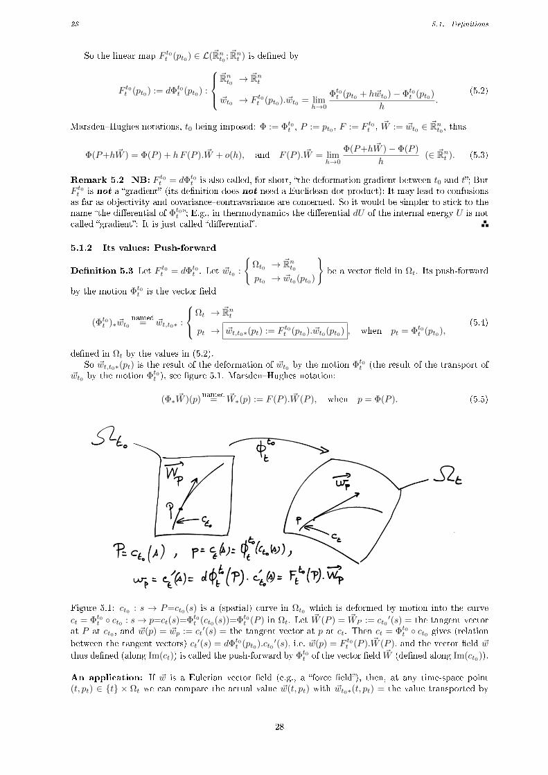
28 5.1. Denitions
So the linear map F t0t (pt0) ∈ L(~Rnt0 ; ~Rnt ) is dened by
F t0t (pt0) := dΦt0t (pt0) :
~Rnt0 → ~Rnt
~wt0 → F t0t (pt0). ~wt0 = limh→0
Φt0t (pt0 + h~wt0)− Φt0t (pt0)
h.
(5.2)
MarsdenHughes notations, t0 being imposed: Φ := Φt0t , P := pt0 , F := F t0t , ~W := ~wt0 ∈ ~Rnt0 , thus
Φ(P+h ~W ) = Φ(P ) + hF (P ). ~W + o(h), and F (P ). ~W = limh→0
Φ(P+h ~W )− Φ(P )
h(∈ ~Rnt ). (5.3)
Remark 5.2 NB: F t0t = dΦt0t is also called, for short, the deformation gradient between t0 and t; ButF t0t is not a gradient (its denition does not need a Euclidean dot product); It may lead to confusionsas far as objectivity and covariancecontravariance are concerned. So it would be simpler to stick to thename the dierential of Φt0t ; E.g., in thermodynamics the dierential dU of the internal energy U is notcalled gradient: It is just called dierential.
5.1.2 Its values: Push-forward
Denition 5.3 Let F t0t = dΦt0t . Let ~wt0 :
Ωt0 → ~Rnt0pt0 → ~wt0(pt0)
be a vector eld in Ωt. Its push-forward
by the motion Φt0t is the vector eld
(Φt0t )∗ ~wt0named
= ~wt,t0∗ :
Ωt → ~Rnt
pt → ~wt,t0∗(pt) := F t0t (pt0). ~wt0(pt0) , when pt = Φt0t (pt0),(5.4)
dened in Ωt by the values in (5.2).So ~wt,t0∗(pt) is the result of the deformation of ~wt0 by the motion Φt0t (the result of the transport of
~wt0 by the motion Φt0t ), see gure 5.1. MarsdenHughes notation:
(Φ∗ ~W )(p)named
= ~W∗(p) := F (P ). ~W (P ), when p = Φ(P ). (5.5)
Figure 5.1: ct0 : s → P=ct0(s) is a (spatial) curve in Ωt0 which is deformed by motion into the curve
ct = Φt0t ct0 : s→ p=ct(s)=Φt0t (ct0(s))=Φt0t (P ) in Ωt. Let ~W (P ) = ~WP := ct0′(s) = the tangent vector
at P at ct0 , and ~w(p) = ~wp := ct′(s) = the tangent vector at p at ct. Then ct = Φt0t ct0 gives (relation
between the tangent vectors) ct′(s) = dΦt0t (pt0).ct0
′(s), i.e. ~w(p) = F t0t (P ). ~W (P ), and the vector eld ~w
thus dened (along Im(ct)) is called the push-forward by Φt0t of the vector eld ~W (dened along Im(ct0)).
An application: If ~w is a Eulerian vector eld (e.g., a force eld), then, at any time-space point(t, pt) ∈ t × Ωt we can compare the actual value ~w(t, pt) with ~wt0∗(t, pt) = the value transported by
28
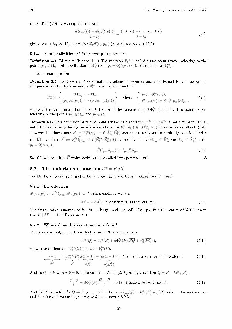
29 5.2. The unfortunate notation d~x = F.d ~X
the motion (virtual value); And the rate
~w(t, p(t))− ~wt0∗(t, p(t))
t− t0=
(actual)− (transported)
t− t0(5.6)
gives, as t→ t0, the Lie derivative L~v ~w(t0, pt0) (rate of stress, see 15.5).
5.1.3 A full denition of F : A two point tensors
Denition 5.4 (MarsdenHughes [12].) The function F t0t is called a two point tensor, referring to thepoints pt0 ∈ Ωt0 (set of denition of Φt0t ) and pt = Φt0t (pt0) ∈ Ωt (arrival set of Φt0t ).
To be more precise:
Denition 5.5 The (covariant) deformation gradient between t0 and t is dened to be the secondcomponent of the tangent map TΦt0t which is the function
TΦt0t :
TΩt0 → TΩt
(pt0 , ~w(pt0)) → (pt, ~wt,t0∗(pt))
where
pt := Φt0t (pt0),
~wt,t0∗(pt) := dΦt0t (pt0). ~wpt0 ,(5.7)
where TΩ is the tangent bundle, cf. 1.8. And the tangent map TΦt0t is called a two point tensor,referring to the points pt0 ∈ Ωt0 and pt ∈ Ωt.
Remark 5.6 This denition of a two point tensor is a shortcut: F t0t := dΦt0t is not a tensor, i.e. is
not a bilinear form (which gives scalar results) since F t0t (pt0) ∈ L(~Rnt0 ; ~Rnt ) gives vector results cf. (5.4).
However the linear map F := F t0t (pt0) ∈ L(~Rnt0 ; ~Rnt ) can be naturally and canonically associated with
the bilinear form F := ˜F t0t (pt0) ∈ L(~Rn∗t , ~Rnt0 ;R) dened by, for all ~upt0 ∈ ~Rnt0 and `pt ∈ ~Rn∗t , with
pt = Φt0t (pt0),
F (`pt , ~upt0 ) := `pt .F.~upt0 . (5.8)
See (T.13). And it is F which denes the so-called two point tensor.
5.2 The unfortunate notation d~x = F.d ~X
Let Ot0 be an origin at t0 and ot be an origin at t, and let ~X =−−−−→Ot0pt0 and ~x = −−→otpt.
5.2.1 Introduction
~wt,t0∗(pt) := F t0t (pt0). ~wt0(pt0) in (5.4) is sometimes written
d~x = F.d ~X : a very unfortunate notation . (5.9)
But this notation amounts to confuse a length and a speed: E.g., you nd the sentence (5.9) is event
true if ||d ~X|| = 1... Explanations:
5.2.2 Where does this notation come from?
The notation (5.9) comes from the rst order Taylor expansion
Φt0t (Q) = Φt0t (P ) + dΦt0t (P ).−−→PQ+ o(||−−→PQ||), (5.10)
which reads when q := Φt0t (Q) and p := Φt0t (P ):
q − p︸ ︷︷ ︸δ~x
= dΦt0t (P )︸ ︷︷ ︸F
.(Q− P︸ ︷︷ ︸δ ~X
) + (o(Q− P ))︸ ︷︷ ︸o(δ ~X)
(relation between bi-point vectors). (5.11)
And as Q→ P we get 0 = 0, quite useless... While (5.10) also gives, when Q = P + h~wt0(P ),
q − ph
= dΦt0t (P ).Q− Ph
+ o(1) (relation between rates). (5.12)
And (5.12) is useful: As Q→ P you get the relation ~wt,t0∗(p) = F t0t (P ). ~wt0(P ) between tangent vectorsand h→ 0 (push-forwards), see gure 5.1 and next 5.2.3.
29
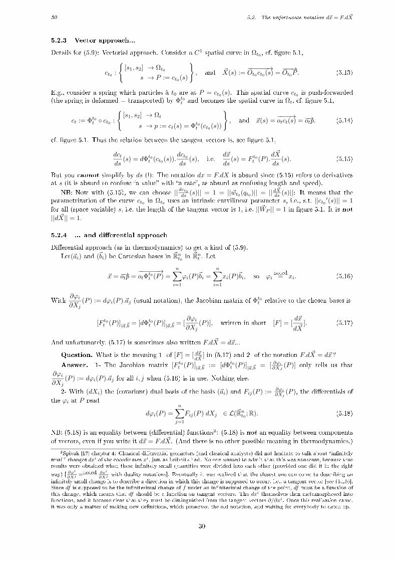
30 5.2. The unfortunate notation d~x = F.d ~X
5.2.3 Vector approach...
Details for (5.9): Vectorial approach. Consider a C1 spatial curve in Ωt0 , cf. gure 5.1,
ct0 :
[s1, s2] → Ωt0
s → P := ct0(s)
, and ~X(s) :=
−−−−−−→Ot0ct0(s) =
−−−→Ot0P . (5.13)
E.g., consider a spring which particles à t0 are at P = ct0(s). This spatial curve ct0 is push-forwarded(the spring is deformed = transported) by Φt0t and becomes the spatial curve in Ωt, cf. gure 5.1,
ct := Φt0t ct0 :
[s1, s2] → Ωt
s → p := ct(s) = Φt0t (ct0(s))
, and ~x(s) =
−−−−→otct(s) = −→otp. (5.14)
cf. gure 5.1. Thus the relation between the tangent vectors is, see gure 5.1,
dctds
(s) = dΦt0t (ct0(s)).dct0ds
(s), i.e.d~x
ds(s) = F t0t (P ).
d ~X
ds(s). (5.15)
But you cannot simplify by ds (!): The notation dx = F.dX is absurd since (5.15) refers to derivativesat s (it is absurd to confuse a value with a rate, as absurd as confusing length and speed).
NB: Now with (5.15), we can choose ||dct0ds (s)|| = 1 = ||~wt0(qt0)|| = ||d ~Xds (s)||: It means that theparametrization of the curve ct0 in Ωt0 uses an intrinsic curvilinear parameter s, i.e., s.t. ||ct0 ′(s)|| = 1
for all (space variable) s, i.e. the length of the tangent vector is 1, i.e. || ~WP || = 1 in gure 5.1. It is not
||d ~X|| = 1.
5.2.4 ... and dierential approach
Dierential approach (as in thermodynamics) to get a kind of (5.9).
Let(~ai) and (~bi) be Cartesian bases in ~Rnt0 in ~Rnt . Let
~x = −→otp =−−−−−−→otΦ
t0t (P ) =
n∑i=1
ϕi(P )~bi =
n∑i=1
xi(P )~bi, so ϕinoted
= xi. (5.16)
With∂ϕi∂Xj
(P ) := dϕi(P ).~aj (usual notation), the Jacobian matrix of Φt0t relative to the chosen bases is
[F t0t (P )]|~a,~b = [dΦt0t (P )]|~a,~b = [∂ϕi∂Xj
(P )], written in short [F ] = [d~x
d ~X]. (5.17)
And unfortunately, (5.17) is sometimes also written F.d ~X = d~x...
Question. What is the meaning 1- of [F ] = [ d~xd ~X
] in (5.17) and 2- of the notation F.d ~X = d~x ?
Answer. 1- The Jacobian matrix [F t0t (P )]|~a,~b := [dΦt0t (P )]|~a,~b = [ ∂ϕi∂XJ(P )] only tells us that
∂ϕi∂Xj
(P ) := dϕi(P ).~aj for all i, j when (5.16) is in use. Nothing else.
2- With (dXi) the (covariant) dual basis of the basis (~ai) and Fij(P ) := ∂ϕi∂Xj
(P ), the dierentials of
the ϕi at P read
dϕi(P ) =
n∑j=1
Fij(P ) dXj ∈ L(~Rnt0 ;R). (5.18)
NB: (5.18) is an equality between (dierential) functions2: (5.18) is not an equality between components
of vectors, even if you write it d~x = F.d ~X. (And there is no other possible meaning in thermodynamics.)
2Spivak [17] chapter 4: Classical dierential geometers (and classical analysts) did not hesitate to talk about innitelysmall changes dxi of the coordinates xi, just as Leibnitz had. No one wanted to admit that this was nonsense, because trueresults were obtained when these innitely small quantities were divided into each other (provided one did it in the right
way) [ ∂ϕi
∂Xj=noted ∂xi
∂Xjwith duality notations]. Eventually it was realized that the closest one can come to describing an
innitely small change is to describe a direction in which this change is supposed to occur, i.e., a tangent vector [see (5.15)].Since df is supposed to be the innitesimal change of f under an innitesimal change of the point, df must be a function ofthis change, which means that df should be a function on tangent vectors. The dxi themselves then metamorphosed intofunctions, and it became clear that they must be distinguished from the tangent vectors ∂/∂xi. Once this realization came,it was only a matter of making new denitions, which preserved the old notation, and waiting for everybody to catch up.
30
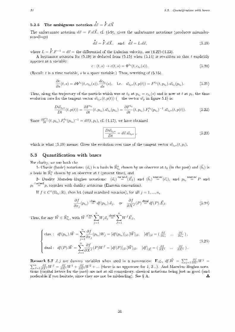
31 5.3. Quantication with bases
5.2.5 The ambiguous notation•
d~x =•
F .d ~X
The unfortunate notation d~x = F.d ~X, cf. (5.9), gives the unfortunate notations (produces misunder-standings)
•
d~x =•
F .d ~X, and•
d~x = L.d~x, (5.19)
where L =•
F .F−1 = d~v = the dierential of the Eulerian velocity, see (4.22)-(4.23).A legitimate notation for (5.19) is deduced from (5.15) when (5.14) is rewritten so that t explicitly
appears as a variable:c : (t, s)→ c(t, s) = Φt0(t, ct0(s)). (5.20)
(Recall: t is a time variable, s is a space variable.) Thus, rewriting of (5.15),
∂c
∂s(t, s) = dΦt0(t, ct0(s)).
dct0ds
(s), i.e. ~wt0∗(t, p(t)) = F t0(t, pt0). ~wt0(pt0). (5.21)
Thus, along the trajectory of the particle which was at t0 at pt0 = ct0(s) and is now at t at pt, the timeevolution rate for the tangent vector ~wt0∗(t, p(t)) (= the vector ~wp in gure 5.1) is:
D~wt0∗Dt
(t, p(t)) =∂F t0
∂t(t, pt0). ~wt0(pt0) =
∂F t0
∂t(t, pt0).F t0t (pt0)−1. ~wt0∗(t, p(t)). (5.22)
Since ∂F t0
∂t (t, pt0).F t0t (pt0)−1 = d~v(t, pt), cf. (4.17), we have obtained
D~wt0∗Dt
= d~v.~wt0∗ , (5.23)
which is what (5.19) means: Gives the evolution over time of the tangent vector ~wt0∗(t, pt).
5.3 Quantication with bases
For clarity, we use both the1- Classic (basic) notations: (~ai) is a basis in ~Rnt0 chosen by an observer at t0 (in the past) and (~bi) is
a basis in ~Rnt chosen by an observer at t (present time), and
2- Duality MarsdenHughes notations: (~ai)named
= ( ~EI) and (~bi)named
= (~ei), and pt0named
= P and
ptnamed
= p, together with duality notations (Einstein convention).
If f ∈ C1(Ωt0 ;R), then let (usual standard notation), for all j = 1, ..., n,
∂f
∂xj(pt0)
clas.= df(pt0).~aj , or
∂f
∂XJ(P )
dual= df(P ). ~EJ . (5.24)
Thus, for any ~W ∈ ~Rnt0 , with ~Wclas.=
n∑j=1
Wj~ajdual=
n∑J=1
W J ~EJ ,
clas. : df(pt0). ~W =
n∑j=1
∂f
∂xj(pt0)Wj = [df(pt0)]|~a.[ ~W ]|~a, [df ]|~a = ( ∂f
∂x1... ∂f
∂xn) ,
dual : df(P ). ~W =
n∑J=1
∂f
∂XJ(P )W J = [df(P )]|~a.[ ~W ]|~a, [df ]|~E = ( ∂f
∂X1 ... ∂f∂Xn ) .
(5.25)
Remark 5.7 J, j are dummy variables when used in a summation: E.g., df. ~W =∑nj=1
∂f∂XjW
j =∑nJ=1
∂f∂XJ
W J = ∂f∂X1W
1 + ∂f∂X2W
2 + ... (there is no uppercase for 1, 2...). And MarsdenHughes nota-tions (capital letters for the past) are not at all compulsory, classical notations being just as good (andpreferable if you hesitate, since they are not be misleading). See A.
31
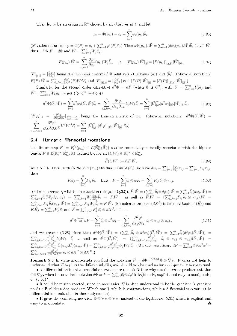
32 5.4. Remark: Tensorial notations
Then let ot be an origin in Rn chosen by an observer at t, and let
pt = Φ(pt0) = ot +
n∑i=1
ϕi(pt0)~bi. (5.26)
(Marsden notations: p = Φ(P ) = ot +∑ni=1ϕ
i(P )~ei.) Thus dΦ(pt0). ~W =∑ni=1(dϕi(pt0). ~W )~bi for all ~W ,
thus, with F = dΦ and ~W =∑nj=1Wj~aj ,
F (pt0). ~W =
n∑i,j=1
∂ϕi∂xj
(pt0)Wj~bi, i.e. [F (pt0). ~W ]|~b = [F (pt0)]|~a,~b.[
~W ]|~a, (5.27)
[F ]|~a,~b = [∂ϕi∂xj] being the Jacobian matrix of Φ relative to the bases (~ai) and (~bi). (Marsden notations:
F (P ). ~W =∑ni,J=1
∂ϕi
∂XJ(P )W J~ei and [F ]|~E,~e = [ ∂ϕ
i
∂XJ] and [F (P ). ~W ]|~E = [F (P )]|~E,~e.[
~W ]|~E .)
Similarly, for the second order derivative d2Φ = dF (when Φ is C2), with ~U =∑nj=1Uj~aj and
~W =∑nk=1Wk~ak we get (for C2 motions)
d2Φ(~U, ~W ) =
n∑i=1
d2ϕi(~U, ~W )~bi =
n∑i,j,k=1
∂2ϕi∂xj∂xk
UjWk~bi =
n∑i=1
[~U ]T|~a.[d2ϕi]|~a.[ ~W ]|~a ~bi, (5.28)
[d2ϕi]|~a = [ ∂2ϕi∂xj∂xk
] j=1,...,nk=1,...,n
being the Hessian matrix of ϕi. (Marsden notations: d2Φ(~U, ~W ) =n∑
i,J,K=1
∂2ϕi
∂XJ∂XKU IW J~ei =
n∑i=1
[~U ]T|~E .[d2ϕi]|~E .[
~W ]|~E ~ei.)
5.4 Remark: Tensorial notations
The linear map F := F t0t (pt0) ∈ L(~Rnt0 ; ~Rnt ) can be canonically naturally associated with the bipoint
tensor F ∈ L(~Rn∗t , ~Rnt0 ;R) dened by, for all (`, ~W ) ∈ ~Rn∗t × ~Rnt0 ,
F (`, ~W ) := `.F. ~W, (5.29)
see A.9.4. Then, with (5.26) and (πai) the dual basis of (~ai), we have dϕi =∑nj=1
∂ϕi∂xj
πaj =∑nj=1Fijπaj ,
thus
F.~aj =
n∑i=1
Fij~bi, thus F =
n∑i=1
~bi ⊗ dϕi =
n∑i,J=1
Fij~bi ⊗ πaj . (5.30)
And we do recover, with the contraction rule (see (Q.23)), F . ~W = (∑ni=1~bi⊗dϕi). ~W =
∑ni=1~bi(dϕi. ~W ) =∑n
i,j=1~bi(Wjdϕi.aj) =
∑ni,J=1Wj
∂ϕi∂xj
~bi = F. ~W . as well as F . ~W = (∑ni,J=1Fij
~bi ⊗ πaj). ~W =∑ni,J=1Fij
~bi(πaj . ~W ) =∑ni,J=1FijWj
~bi = F. ~W . (Marsden notations: (dXI) is the dual basis of ( ~EI) and
F. ~EJ =∑ni=1F
iJ ~ei and F =
∑ni,J=1F
iJ ~ei ⊗ dXJ .) Then
d2Φisom' dF =
n∑i=1
~bi ⊗ d2ϕi =
n∑i,j,k=1
∂2ϕi
∂xj∂xk~bi ⊗ πaj ⊗ πak, (5.31)
and we recover (5.28) since then d2Φ(~U, ~W ) = (∑ni=1~bi ⊗ d2ϕi)(~U, ~W ) =
∑ni=1~bi(d
2ϕi(~U, ~W )) =∑ni,j,k=1
∂2ϕi
∂xj∂xkUjWk
~bi as well as d2Φ(~U, ~W ) = (∑ni,j,k=1
∂2ϕi
∂xj∂xk~bi ⊗ πaj ⊗ πak)(~U, ~W ) =∑n
i,j,k=1∂2ϕi
∂xj∂xk~bi(πaj .~U)(πak. ~W ) =
∑ni,j,k=1
∂2ϕi
∂xj∂xkUjWk
~bi. (Marsden notations: dF =∑ni=1~ei⊗d2ϕi =∑n
i,J,K=1∂2ϕi
∂XJ∂XK~ei ⊗ dXJ ⊗ dXK .)
Remark 5.8 In some manuscripts you nd the notation F = dΦ =noted Φ ⊗ ∇X . It does not help tounderstand what F is (it is the dierential dΦ), and should not be used as far as objectivity is concerned:• A dierentiation is not a tensorial operation, see remark R.1, so why use the tensor product notation
Φ⊗∇X , when the standard notation dΦ ' F =∑ni=1~ei⊗dϕi is legitimate, explicit and easy to manipulate,
cf. (5.30)?• It could be misinterpreted, since, in mechanics, ∇ is often understood to be the gradient (a gradient
needs a Euclidean dot product: Which one?) which is contravariant, while a dierential is covariant (adierential is unmissable in thermodynamics).• It gives the confusing notation Φ⊗∇X ⊗∇X , instead of the legitimate (5.31) which is explicit and
easy to manipulate.
32
33 5.5. Change of coordinate system at t for F
5.5 Change of coordinate system at t for F
Let pt0 ∈ Ωt0 , let pt = Φt0t (pt0), let ~W (pt0) ∈ ~Rnt0 , let ~w(pt) = F t0t (pt0). ~W (pt0) ∈ ~Rnt (its push-forward),
written ~w = F. ~W for short.At the actual time t, we are interested in the result seen by two observers, the rst using a Cartesian
basis (~b1i), the second using a Cartesian basis (~b2i): Both bases are in ~Rnt . Let P = [Pij ] be the transition
matrix from (~b1i) to (~b2i), that is, ~b2j =∑ni=1Pij
~b1i for all j.
The change of basis formula for vectors from (~b1i) to (~b2i) (in ~Rnt ) applied to ~w ∈ ~Rnt gives
[~w]|~b2 = P−1.[~w]|~b1 , thus [F. ~W ]|~b2 = P−1.[F. ~W ]|~b1 . (5.32)
Thus, with (~ai) a basis in ~Rnt0 chosen by some observer in the past, we get
[F ]|~a,~b2 .[~W ]|~a = P−1.[F ]|~a,~b1 .[
~W ]|~a, (5.33)
true for all ~W , thus
[F ]|~a,~b2 = P−1.[F ]|~a,~b1 . (5.34)
NB: (5.34) is not the change of coordinate system formula for an endomorphism, which would be nonsense
since F := F t0t (pt0) : ~Rnt0 → ~Rnt is not an endomorphism, cf. (5.7): (5.34) is the usual change of basis
formula for vectors in ~Rnt , cf. (5.32).
5.6 Spatial Taylor expansion of Φt0t and F t0
t
Φt0t is supposed to be C1 for all t0, t. Let pt0 ∈ Ωt0 and ~Wpt0∈ ~Rnt0 . Then
Φt0t (pt0+h ~Wpt0) = Φt0t (pt0) + h dΦt0t (pt0). ~Wpt0
+ o(h)
= Φt0t (pt0) + hF t0t (pt0). ~Wpt0+ o(h).
(5.35)
And, with Φt0t C2,
Φt0t (pt0+h ~Wpt0) = Φt0t (pt0) + h dΦt0t (pt0). ~Wpt0
+h2
2d2Φt0t (pt0)( ~Wpt0
, ~Wpt0) + o(h2)
= Φt0t (pt0) + hF t0t (pt0). ~Wpt0+h2
2dF t0t (pt0)( ~Wpt0
, ~Wpt0) + o(h2).
(5.36)
AndF t0t (pt0+h ~Wpt0
) = F t0t (pt0) + h dF t0t (pt0). ~Wpt0+ o(h) ∈ L(~Rnt0 ; ~Rnt ), (5.37)
that is, for any ~Upt0 ∈ ~Rnt0 ,
F t0t (pt0+h ~Wpt0).~Upt0 = F t0t (pt0).~Upt0 + h (dF t0t (pt0). ~Wpt0
).~Upt0 + o(h) ∈ ~Rnt , (5.38)
with (dF t0t (pt0). ~Wpt0).~Upt0 = d2Φt0t (pt0)( ~Wpt0
, ~Upt0 ).
5.7 Time Taylor expansion of F t0pt0
Let Φ be a C2 motion of Obj , let t0 ∈ R, and let Φt0 be the associated motion. The time Taylorexpansion of Φt0t is given in (4.31)-(4.32). So, with pt = Φ(t, PObj ) and pt0 = Φ(t0, PObj ), with ~v(t, pt) =∂Φ∂t (t, PObj ) the Eulerian velocity and ~V t0(t, pt0) := ∂Φt0
∂t (t, pt0) = ~v(t, pt) the Lagrangian velocity, andwith F t0(t, pt0) = dΦt0(t, pt0), we have
(F t0pt0 )′(t) =∂(dΦt0)
∂t(t, pt0) = d(
∂Φt0
∂t)(t, pt0) =
∂F t0
∂t(t, pt0) =
∂(dΦt0)
∂t(t, pt0)
= d~V t0(t, pt0) = d~v(t, p(t)).F t0pt0 (t).
(5.39)
Short abusive notation: F ′ = d~v.F (at what points, what times?), or•
F = d~v.F (= d~V ).
33
34 6.1. Introduction: Motion versus ow
If Φt0 is C3 then ∂2Φt0
∂t2 (t, pt0) = ~At0(t, pt0) = ~γ(t, p(t)) (Lagrangian and Eulerian accelerations), hence
(F t0pt0 )′′(t) = d ~At0(t, pt0) = d~γ(t, pt).Ft0pt0
(t). (5.40)
Short abusive notation: F ′′ = d~γ.F (at what points, what times?), or••
F = d~γ.F (= d ~A).Thus, the second order time Taylor expansion of F t0pt0 is
F t0pt0 (t+h) =(F t0pt0 + h d~V t0pt0 +
h2
2d ~At0pt0
)(t) + o(h2)
=(I + h d~v +
h2
2d~γ)
(t, p(t)).F t0pt0 (t) + o(h2) when p(t) = Φt0(t, pt0).
(5.41)
NB: they are three times are involved: t0 (observer dependent), t and t+h, as for (4.31).In particular, F t0t0 (pt0) = I gives
F t0pt0 (t0+h) =(I + h d~v +
h2
2d~γ)(t0, pt0) + o(h2) (5.42)
Remark 5.9 γ = ∂~v∂t + d~v.~v is not linear in ~v. Idem,
d~γ = d(D~v
Dt) = d(
∂~v
∂t+ d~v.~v) = d
∂~v
∂t+ d2~v.~v + d~v.d~v (=
D(d~v)
Dt+ d~v.d~v) (5.43)
is non linear in ~v, and gives F t0pt0′′(t) = (d∂~v∂t + d2~v.~v + d~v.d~v)(t, pt).F
t0pt0
(t), non linear in ~v.
Exercice 5.10 Directly check that F ′ = d~v.F gives F ′′ = d~γ.F .
Answer. F ′(t) = d~v(t, p(t)).F (t) gives F ′′(t) = D(d~v)Dt
(t, p(t)).F (t) + d~v(t, p(t)).F ′(t) with D(d~v)Dt
= d~γ − d~v.~v,cf. (5.43), thus F ′′(t) = (d~γ − d~v.d~v)(t, p(t)).F (t) + d~v(t, p(t)).d~v(t, p(t)).F (t) = d~γ(t, p(t)).F (t).
6 Flow
6.1 Introduction: Motion versus ow
• A motion Φ : (t, PObj )→ pt = Φ(t, PObj ) locates a particle PObj at t in the ane space Rn, cf. (1.5),
and the Eulerian velocity eld ~v of the particle is ~v(t, pt) :=dΦPObj
dt (t, PObj ) when pt = Φ(t, PObj ), cf. (2.5).• A ow starts from a Eulerian velocity eld ~v to deduce a motion by solving the ODE (ordinary
dierential equation) dΦdt (t) = ~v(t,Φ(t)) (with CauchyLipschitz theorem). In particular, a ow doesn't
deal with Lagrangian velocities (two point tensors): It deals with ODEs and Eulerian velocities (tensors).
6.2 Denition
Let ~v :
R× Rn → ~Rn
(t, p) → ~v(t, p)
be a unstationary vector eld (e.g., a Eulerian velocity eld). We look
for maps Φ :
R → Ω
t → p = Φ(t)
which are locally (i.e. in the vicinity of some t) solutions of the ODE
(ordinary dierential equation)
dΦ
dt(t) = ~v(t,Φ(t)), also written
dp
dt(t) = ~v(t, p(t)). (6.1)
(Also written d~xdt (t) = ~v(t, ~x(t)) with ~x(t) =
−−−→Op(t), cf. (1.6).)
Denition 6.1 A solution Φ of (6.1) is a ow of ~v; Also called an integral curve of ~v, since Φ(τ) =∫ τu=t
~v(u,Φ(u)) du+ Φ(t).
Remark 6.2 Improper notation for (6.1):
dp
dt(t)
noted=
dp(t)
dt(= ~v(t, p(t))). (6.2)
Question: If the notation dp(t)dt is used, then what is the meaning of dp(f(t))
dt ?
Answer: It means, either dpdt (f(t)), or d(pf)
dt (t) = dpdt (f(t))dfdt (t): Ambiguous. So it is better to use
dpdt (t), and to avoid dp(t)
dt , unless the context is clear (no composite functions).
34
35 6.3. CauchyLipschitz theorem
Remark 6.3 Another improper notation for (6.1): dpdt = ~v(t, p), which does not mean dp
dt (u) = ~v(t, p(u))
for any u, but dpdt (t) = ~v(t, p(t)). (The notation dp
du (u) = ~v(t, p(u)) is used for streamlines, cf. (2.21).)
6.3 CauchyLipschitz theorem
Let (t0, pt0) be in the denition domain of ~v (and (t0, pt0) will be called an initial condition). We lookfor Φ solution of
dΦ
dt(t) = ~v(t,Φ(t)) and Φ(t0) = pt0 , (6.3)
which is an ODE (Ordinary Dierential Equation) with an initial condition.
Denition 6.4 Let t1, t2 ∈ R, t1 < t2. Let Ω be an open set in Rn and Ω its closure. Let ||.|| be a normin ~Rn. A continuous map ~v : [t1, t2] × Ω → ~Rn is Lipschitzian i it is space Lipschitzian, uniformly intime, that is, i
∃k > 0, ∀t ∈ [t1, t2], ∀p, q ∈ Ω, ||~v(t, q)− ~v(t, p)|| ≤ k||q − p||. (6.4)
That is, ||~vt(q)−~vt(p)||||q−p|| ≤ k, for all t and all p 6= q, That is, the variations of ~v are bounded in space,
uniformly in time.
Theorem 6.5 (and denion) (CauchyLipschitz). Let ~v : [t1, t2]×Ω→ ~Rn be Lipschitzian, cf. (6.4),and let (t0, pt0) ∈]t1, t2[×Ω. Then there exists ε = εt0,pt0 > 0 s.t. (6.3) has a unique solution Φ :]t0−ε, t0+ε[→ Rn, which is called a ow of ~v (more precisely, is called the ow of ~v which satisesΦ(t0) = pt0).
Moreover, if ~v is Ck then Φ is Ck+1.
Proof. See e.g. Arnold [2], or any ODE course. In particular ||~v||∞ := supt∈]t0−ε,t0+ε[, p∈Ω
||~v(t, p)||Rn
(maximum speed) exists since ~v ∈ C0 on the compact [t1, t2]×Ω), see denition 6.4, hence we can choose
ε = min(t0−t1, t2−t0,d(pt0 ,∂Ω)
||~v||∞ ) (the time needed to reach the border ∂Ω from pt0).
Notations. The solution Φ of (6.3) is noted Φt0pt0 : So, for all t ∈]t0−ε, t0+ε[,
dΦt0pt0dt
(t) = ~v(t,Φt0pt0 (t)) and Φt0pt0 (t0) = pt0 . (6.5)
We have thus dened for some Ωt0 ⊂ Ω (see next theorem 6.6),
Φt0 :
[t0−ε, t0+ε]× Ωt0 → Rn
(t, pt0) → p = Φt0(t, pt0) := Φt0pt0 (t) :(6.6)
The function Φt0 is also called a ow. And (6.5) reads
∂Φt0
∂t(t, pt0) = ~v(t,Φt0(t, pt0)), and Φt0(t0, pt0) = pt0 . (6.7)
We have thus dened,
Φ :
]t1, t2[×]t1, t2[×Ωt0 → Ω
(t, t0, pt0) → p = Φ(t, t0, pt0) := Φt0pt0 (t)noted
= Φ(t; t0, pt0).(6.8)
The function Φ is also called a ow. And (6.5) reads
∂Φ
∂t(t; t0, pt0) = ~v(t,Φ(t; t0, pt0)), with Φ(t0; t0, pt0) = pt0 . (6.9)
Other notation: Φt;t0 := Φt0t : Ωt0 → Rn, and (6.9) is also written
dΦt;t0(pt0)
dt= ~v(t,Φt;t0(pt0)), and Φt;t0(pt0) = pt0 . (6.10)
Theorem 6.6 Let ~v be Lipschitzian, cf. (6.4). Let t0 ∈]t1, t2[, and let Ωt0 be an open set s.t. Ωt0 ⊂⊂ Ω,that is, there exists a compact set K ∈ Rn s.t. Ωt0 ⊂ K ⊂ Ω. Then there exists ε > 0 s.t. a ow Φt0
exists on ]t0−ε, t0+ε[×Ωt0 , cf. (6.6).
35
36 6.4. Examples
Proof. Let d = d(K,Rn−Ω) (la distance of K to the border of Ω.Let ||~v||∞ := sup
t∈[t1,t2],p∈Ω
||~v(t, p)||Rn (exists since ~v ∈ C0 on the compact [t1, t2]× Ω).
Let ε = min(t0−t1, t2−t0, d||~v||∞ ) (less that the minimum time to reach the border fromK at maximum
speed ||v||∞).Let P ∈ K and t ∈]t0−ε, t0+ε[. Then Φt0P exists, cf.theorem 6.5, and ||Φt0P (t) − Φt0P (t0)||Rn ≤ [t −
t0| supτ∈]t0−ε,t0+ε[(||(Φt0P )′(τ)||Rn) (mean value theorem since, ~v being C0, Φt0P is C1). Thus ||Φt0P (t) −
Φt0P (t0)||Rn ≤ [t − t0| ||v||∞, thus Φt0P (t) ∈ Ω. Thus Φt0P exists on ]t0−ε, t0+ε[, for all P ∈ K. Thus Φt0
exists on ]t0−ε, t0+ε[×K.
Remark 6.7 The (Eulerian) approach of a ow starts with a Eulerian type velocity (independent ofany initial time), and then, due to the introduction of initial conditions, leads to Lagrangian functions,cf. (6.5). Once again, Lagrangian functions are the result of Eulerian functions: And in this manuscriptwe were careful to introduce 2 (Eulerian) before 4 (Lagrangian).
6.4 Examples
Example 1 R2 with an origin O and a Euclidean basis (~e1, ~e2). Let p ∈ R2,−→Op=noted ~x = x~e1 +
y~e2 =noted(x, y). Let t1 = −1, t2 = 1 and Ω = [0, 2] × [0, 1] (observation window). Let t0 ∈]t1, t2[,a, b ∈ R, a 6= 0, and consider
~v(t, p) =
v1(t, x, y) = ay,
v2(t, x, y) = b sin(t−t0).(6.11)
(b = 0 corresponds to the stationary case = shear ow.) So ~v is a C∞ vector eld.
Then (6.7) reads, with ~x(t0) = (x0, y0) and ~x(t) =−−−−−−→OΦt0pt0 (t) =noted
(x(t)y(t)
),
dx
dt(t) = v1(t, x(t), y(t)) = ay(t), x(t0) = x0,
dy
dt(t) = v2(t, x(t), y(t)) = b sin(t−t0), y(t0) = y0.
(6.12)
Thus−−−→Op(t) =
−−−−−−→OΦt0pt0 (t) =
x(t) = x0 + a(y0 + b)(t−t0)− ab sin(t−t0),
y(t) = y0 + b− b cos(t−t0).(6.13)
Example 2 R2 with an origin O and a Euclidean basis (~e1, ~e2). Let−→Op=noted ~x =
(xy
), let ω > 0
and consider
~v(t, x, y) =
(−ωyωx
)= ω
(0 −11 0
)(xy
)noted
= ~v(x, y). (6.14)
(Spin vector eld.) With−−→Opt0 = ~xt0 =
(xt0yt0
), with rt0 =
√x2t0 + y2
t0 and with θ0 such that ~xt0 =(xt0 = rt0 cos(ωt0)yt0 = rt0 sin(ωt0)
), the solution Φt0pt0 of (6.7) is
−−−→Op(t) =−−−−−−→OΦt0pt0 (t) = ~x(t) =
(x(t) = rt0 cos(ωt)y(t) = rt0 sin(ωt)
). (6.15)
Indeed,
( ∂x∂t (t, ~x0)∂y∂t (t, ~x0)
)=
(v1(t, x(t, ~x0), y(t, ~x0))v2(t, x(t, ~x0), y(t, ~x0))
)=
(−ωy(t, ~x0)ωx(t, ~x0)
), thus ∂x
∂t (t, ~x0) = −ωy(t, ~x0)
and ∂y∂t (t, ~x0) = ωx(t, ~x0), thus ∂2y
∂t2 (t, ~x0) = −ω2y(t, ~x0), hence y; Idem for x. Here d~v(t, x, y) =
ω
(0 −11 0
)= ω
(cos π2 − sin π
2sin π
2 cos π2
)is the π/2-rotation composed with the homothety with ratio ω.
6.5 Composition of ows
Let ~v be a vector eld on R× Ω and Φt0pt0 solution of (6.5). We use the notations
pt = Φt0t (pt0) = Φt;t0(pt0) := Φt0pt0 (t) = Φt0(t, pt0) = Φ(t; t0, pt0). (6.16)
36
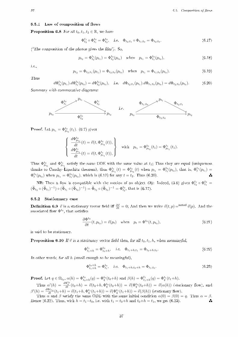
37 6.5. Composition of ows
6.5.1 Law of composition of ows
Proposition 6.8 For all t0, t1, t2 ∈ R, we have
Φt1t2 Φt0t1 = Φt0t2 , i.e. Φt2;t1 Φt1;t0 = Φt2;t0 . (6.17)
(The composition of the photos gives the lm). So,
pt2 = Φt1t2(pt1) = Φt0t2(pt0) when pt1 = Φt0t1(pt0), (6.18)
i.e.,pt2 = Φt2;t1(pt1) = Φt2;t0(pt0) when pt1 = Φt1;t0(pt0). (6.19)
ThusdΦt1t2(pt1).dΦt0t1(pt0) = dΦt0t2(pt0), i.e. dΦt2;t1(pt1).dΦt1;t0(pt0) = dΦt2;t0(pt0). (6.20)
Summary with commutative diagrams:
pt1Φt1t2
''pt0
Φt0t177
Φt0t2
// pt2
i.e.
pt1Φt2;t1
''pt0
Φt1;t0
77
Φt2;t0
// pt2
Proof. Let pt1 = Φt0pt0 (t1). (6.7) givesdΦt0pt0dt
(t) = ~v(t,Φt0pt0 (t)),
dΦt1pt1dt
(t) = ~v(t,Φt1pt1 (t)),
with pt1 = Φt0pt0 (t1) = Φt1pt1 (t1).
Thus Φt0pt0 and Φt1pt1 satisfy the same ODE with the same value at t1; Thus they are equal (uniqueness
thanks to CauchyLipschitz theorem), thus Φt1pt1 (t) = Φt0pt0 (t) when pt1 = Φt0t1(pt0), that is, Φt1t (pt1) =
Φt0t (pt0) when pt1 = Φt0t1(pt0), which is (6.17) for any t = t2. Thus (6.20).
NB: Then a ow is compatible with the motion of an object Obj : Indeed, (3.6) gives Φt1t2 Φt0t1 =
(Φt2 (Φt1)−1) (Φt1 (Φt0)−1) = Φt2 (Φt0)−1 = Φt0t2 , that is (6.17).
6.5.2 Stationnary case
Denition 6.9 ~v is a stationary vector eld i ∂~v∂t = 0; And then we write ~v(t, p) =noted ~v(p). And the
associated ow Φt0 , that satises
∂Φt0
∂t(t, pt0) = ~v(pt) when pt = Φt0(t, pt0), (6.21)
is said to be stationary.
Proposition 6.10 If ~v is a stationary vector eld then, for all t0, t1, h, when meaningful,
Φt1t1+h = Φt0t0+h, i.e. Φt1+h;t1 = Φt0+h;t0 . (6.22)
In other words, for all h (small enough to be meaningful),
Φt0+ht1+h = Φt0t1 , i.e. Φt1+h;t0+h = Φt1;t0 . (6.23)
Proof. Let q ∈ Ωt0 , α(h) = Φt0t0+h(q) = Φt0q (t0+h) and β(h) = Φt1t1+h(q) = Φt1q (t1+h).
Thus α′(h) =dΦt0qdt (t0+h) = ~v(t0+h,Φt0q (t0+h)) = ~v(Φt0q (t0+h)) = ~v(α(h)) (stationary ow), and
β′(h) =dΦt1qdt (t1+h) = ~v(t1+h,Φt1q (t1+h)) = ~v(Φt1q (t1+h)) = ~v(β(h)) (stationary ow).
Thus α and β satisfy the same ODE with the same initial condition α(0) = β(0) = q. Thus α = β.Hence (6.22). Thus, with h = t1−t0, i.e. with t1 = t0+h and t0+h = t1, we get (6.23).
37
38 6.6. Velocity on the trajectory traveled in the opposite direction
Corollary 6.11 If ~v is a stationary vector eld, cf. (6.21), then
dΦt0t (pt0).~v(pt0) = ~v(pt) when pt = Φt0t (pt0), (6.24)
that is, if ~v is stationary, then ~v is transported along itself (see the push-forward 10.5.2).
Proof. Φt0+st+s Φt0t0+s = Φt0t+s, cf. (6.17). Thus, ~v being stationary, Φt0t Φt0t0+s = Φt0t+s, cf. (6.23). That
is, Φ(t; t0, (Φ(t0+s; t0, pt0)) = Φ(t+s; t0, pt0). Thus (s derivative)
dΦ(t; t0,Φ(t0+s; t0, pt0)).∂Φ
∂s(t0+s; t0, pt0) = ~v(t+s,Φ(t+s; t0, pt0))
(see 6.7.1 for non ambiguous calculations), thus (stationary ow) :
dΦt0t (Φt0t0+s(pt0)).~v(Φt0t0+s(pt0)) = ~v(Φt0t+s(pt0)).
And pt = Φt0t (pt0) and s = 0 give (6.24).
6.6 Velocity on the trajectory traveled in the opposite direction
Let t0, t1 ∈ R, t1 > t0, and pt0 ∈ Rn. Consider the trajectory Φt0pt0 :
[t0, t1] → Rn
t → p(t) = Φt0pt0 (t)
. So pt0
is the beginning of the trajectory, pt1 = Φt0t1(pt0) the end, and ~v(t, p(t)) =dΦt0pt0dt (t) the velocity.
Dene the trajectory traveled in the opposite direction by
Ψt1pt1
:
[t0, t1] → Rn
u → q(u) = Ψt1pt1
(u) := Φt0pt0 (t0+t1−u) = Φt0pt0 (t) = p(t) when t = t0+t1−u.(6.25)
In particular q(t0) = Ψt1pt1
(t0) = Φt0pt0 (t1) = p(t1) and q(t1) = Ψt1pt1
(t1) = Φt0pt0 (t0) = p(t0).
Proposition 6.12 The velocity on the trajectory traveled in the opposite direction is the opposite ofthe velocity on the initial trajectory:
dΨt1pt1
du(u) = q′(u) = −p′(t) = −~v(t, p(t)) when t = t0+t1−u, (6.26)
Proof. Ψt1pt1
(u) = Φt0pt0 (t0+t1−u) givesdΨt1pt1du (u) = −
dΦt0pt0dt (t0+t1−u) = −~v(t0+t1−u,Φt0pt0 (t0+t1−u)) =
−~v(t,Φt0pt0 (t)) when t = t0+t1−u.
6.7 Variation of the ow as a function of the initial time
6.7.1 Ambiguous and non ambiguous notations
Let Φ : (t, u, p) ∈ R× R× Rn → Φ(t, u, p) ∈ Rn be a C1 function. The partial derivatives are
∂1Φ(t, u, p) := limh→0
Φ(t+h, u, p)− Φ(t, u, p)
h, (6.27)
∂2Φ(t, u, p) := limh→0
Φ(t, u+h, p)− Φ(t, u, p)
h, (6.28)
and ∂3Φ(t, u, p) dened by, for all ~w ∈ ~Rn (a vector at p),
∂3Φ(t, u, p). ~w := limh→0
Φ(t, u, p+h~w)− Φ(t, u, p)
h
noted= dΦ(t, u, p). ~w, (6.29)
When the name of the rst variable is systematically noted t, then
∂1Φ(t, u, p)noted
=∂Φ
∂t(t, u, p)
noted=
∂Φ(t, u, p)
∂t. (6.30)
NB: This notation can be ambiguous: What is the meaning of ∂Φ∂t (t; t, p)? In ambiguous situations, we
use the notation ∂1Φ.
38
39 7.1. Rate of deformation tensor and spin tensor
When the name of the second variable is systematically noted u, then
∂2Φ(t, u, p)noted
=∂Φ
∂u(t, u, p)
noted=
∂Φ(t, u, p)
∂u. (6.31)
NB: This notation can be ambiguous: What is the meaning of ∂Φ∂u (u;u, p)? In ambiguous situations, we
use the notation ∂2Φ.When the name of the third variable is systematically noted p, then
∂3Φ(t, u, p)noted
=∂Φ
∂p(t, u, p)
noted=
∂Φ(t, u, p)
∂p
noted= dΦ(t, u, p). (6.32)
Since p is the only space variable, the notation ∂Φ∂p is less ambiguous than ∂Φ
∂t (t1, t2, p).
6.7.2 Variation of the ow as a function of the initial time
(6.7), that is, ∂Φ∂t (t;u, q) = ~v(t,Φ(t;u, q)) with Φ(u;u, q) = q for any (u, q) ∈ R× R3, reads
∂1Φ(t;u, q) = ~v(t,Φ(t;u, q)) with Φ(u;u, q) = q. (6.33)
The law of composition of the ows give, cf. (6.19),
Φ(t;u,Φ(u; t0, q)) = Φ(t; t0, q). (6.34)
Thus the derivative in u gives, cf. 6.7.1 (non ambiguous)
∂2Φ(t;u,Φ(u; t0, q)) + dΦ(t;u,Φ(u; t0, q)).∂1Φ(u; t0, q) = 0,
i.e. ∂2Φ(t;u,Φ(u; t0, q)) + dΦ(t;u,Φ(u; t0, q)).~v(u,Φ(u; t0, q)) = 0,
written∂Φ
∂u(t;u, p) + dΦ(t;u, p).~v(u, p) = 0 with p = Φ(u; t0, p) = pu.
(6.35)
(Or, ambiguous, ∂Φ(t;u,p(u))∂u = −dΦ(t;u, p(u)).~v(u, p(u)).) Thus u = t0 and Φ(t0; t0, pt0) = pt0 give
∂2Φ(t; t0, pt0) = −dΦ(t; t0, pt0).~v(t0, pt0),
written∂Φ
∂t0(t; t0, pt0) = −dΦ(t; t0, pt0).~v(t0, pt0).
(6.36)
(Or, ambiguous,∂Φ(t;t0,pt0 )
∂t0= −dΦ(t; t0, pt0).~v(t0, pt0).)
In particular ∂2Φ(t0; t0, pt0) = −~v(t0, pt0), i.e. ∂Φ∂t0
(t; t0, pt0) = −~v(t0, pt0). (Or, ambiguous,dΦ(t;t0,pt0 )
dt0 |t=t0= −~v(t0, pt0).
7 Decomposition of d~v
Let Φ : [t1, t2] × Obj → Rn be a regular motion, cf. (1.5), and let ~v : C → ~Rn be the Eulerian velocity
eld, cf. (2.5), that is, ~v(t, p) = ∂Φ∂t (t, PObj ) when p = Φ(t, PObj ). Its dierential d~v is given in (2.10).
A observer chooses a unit of measurement (foot, meter...) and builds the associated Euclidean dotproduct (·, ·)g, cf. B.2.
7.1 Rate of deformation tensor and spin tensor
Thanks to a chosen Euclidean dot product (·, ·)g in ~Rnt , we can consider the transposed endomorphism
d~vt(p)Tg =noted d~vt(p)
T ∈ L(~Rnt ; ~Rnt ): It is given by, for all ~w1, ~w2 ∈ ~Rnt vectors at p,
(d~vt(p)T . ~w1, ~w2)g = (~w1, d~vt(p). ~w2)g (7.1)
cf. A.7. And we use the usual notations (denitions)
d~vTt (p) := d~vt(p)T noted
= d~vT (t, p)noted
= d~v(t, p)T . (7.2)
39
40 7.2. Quantication with a basis
Denition 7.1 The (Eulerian) rate of deformation tensor, or stretching tensor, is the (Euclidean) sym-metrical part of d~v, that is, the Eulerian map
D =d~v + d~vT
2, i.e., ∀(t, p) ∈
⋃t∈R
(t × Ωt), D(t, p) =d~v(t, p) + d~v(t, p)T
2. (7.3)
And the (Eulerian) spin tensor is the antisymmetric part of d~v, that is,
Ω =d~v − d~vT
2, i.e., ∀(t, p) ∈
⋃t∈R
(t × Ωt), Ω(t, p) =d~v(t, p)− d~v(t, p)T
2. (7.4)
Sod~v = D + Ω. (7.5)
NB: the same notation will be used for the set Ωt = Φt0t (Ωt0) ⊂ Rn and for the spin tensor Ωt =d~vt−d~vTt
2
given by Ωt(p) = d~vt(p)−d~vt(p)T2 , cf. (7.4): The context removes ambiguities.
7.2 Quantication with a basis
Consider a basis (~ei) in ~Rnt . (7.1) then gives [g]|~e.[d~vT ]|~e = [d~v]T|~e.[g]|~e.
In particular, if (~ei) is a (·, ·)g-orthonormal basis (a (·, ·)g Euclidean basis), then [g]|~e = I and [d~vT ]|~e =
[d~v]T|~e. That is, if ~v =∑ni=1vi~ei, then d~v.~ej =
∑ni=1
∂vi∂xj
~ei, then d~vT .~ej =
∑ni=1
∂vj∂xi
~ei, that is,
[d~v]|~e = [∂vi∂xj
] i=1,...,nj=1,...,n
Euclidean framework=⇒ [d~vT ]|~e = [
∂vj∂xi
] i=1,...,nj=1,...,n
= [d~v]T|~e. (7.6)
Thus for the endomorphisms D and Ω, and with D.~ej =∑ni=1Dij~ei and Ω.~ej =
∑ni=1Ωij~ei, we get
Dij = 12 ( ∂vi∂xj
+∂vj∂xi
) and Ωij = 12 ( ∂vi∂xj
− ∂vj∂xi
), that is,
[D]|~e =[d~v]|~e + [d~v]T|~e
2and [Ω]|~e =
[d~v]|~e − [d~v]T|~e
2(Euclidean framework). (7.7)
With duality notations, ~v =∑ni=1v
i~ei and d~v.~ej =∑ni=1
∂vi
∂xj ~ei, thus d~vT .~ej =
∑ni=1
∂vj
∂xi~ei: The
Einstein convention is not satised in d~vT .~ej =∑ni=1
∂vj
∂xi~ei; Indeed the quantity d~vT is not objectivebecause of the use of the inner dot product (·, ·)g (observer dependent). If you do want to use Einstein's
convention, you have to use [g]|~e.[d~vT ]|~e = [d~v]|~e.[g]|~e, i.e.
∑nk=1gik(d~vT )kj =
∑nk=1
∂vi
∂xkgkj , even if gij = δij .
8 Interpretation of the rate of deformation tensor
We are interested in the evolution of the deformation gradient along the trajectory of a particle PObj
which was at pt0 at t0. So:
Let Φ : [t1, t2] × Obj → Rn be a regular motion, cf. (1.5), t0 ∈ [t1, t2], Ωt0 = Φ(t0,Obj ), PObj ∈ Obj ,
pt0 = Φ(t0, PObj ), Φt0pt0 : t ∈ [t1, t2]→ p(t) = Φt0pt0 (t) = Φ(t, PObj ) ∈ Rn (trajectory of PObj ), cf. (3.8). And
name F (t) := F t0pt0 (t) = dΦt0(t, pt0) := dΦt0t (pt0), cf. (5.2).
Let ~A = ~a(t0, pt0) and ~B = ~b(t0, pt0) be vectors at t0 at pt0 in Ωt0 , and consider their push-forwardsby the ow Φt0t (the transported vectors along a trajectory)
~a(t, p(t)) = F t0(t, pt0). ~A and ~b(t, p(t)) = F t0(t, pt0). ~B, (8.1)
see (5.4) and gure 5.1: Dene the Eulerian scalar function
(~a,~b)g :
C → R
(t, pt) → (~a,~b)g(t, pt) := (~a(t, pt),~b(t, pt))g (= (F (t). ~A, F (t). ~B)g).(8.2)
Proposition 8.1 The rate of deformation tensor D = d~v+d~vT
2 gives (half) the evolution rate between twovectors deformed by the ow, that is, along trajectories,
D(~a,~b)gDt
= 2(D.~a,~b)g. (8.3)
40
41 9.1. Ane motions and rigid body motions
Proof. Let F t0pt0 = F and f(t) := (~a,~b)g(t, p(t)) = (F (t). ~A, F (t). ~B)g where p(t) = Φt0t (pt0); Thus
f ′(t) = (F ′(t). ~A, F (t). ~B)g + (F (t). ~A, F ′(t). ~B)g. (8.4)
And F ′(t) = d~v(t, p(t)).F (t), cf. (4.21). Thus
f ′(t) = (d~v(t, p(t)).F (t). ~A, F (t). ~B)g + (F (t). ~A, d~v(t, p(t)).F (t). ~B)g
= (d~v(t, p(t)).~a(t, p(t)),~b(t, p(t)))g + (~a(t, p(t)), d~v(t, p(t)).~b(t, p(t)))g
= ((d~v(t, p(t)) + d~v(t, p(t))T ).~a(t, p(t)),~b(t, p(t)))g,
(8.5)
i.e. (8.3).
9 Rigid body motions and the spin tensor
The need of Euclidean dot products is required to characterize a rigid body motion. So consider aEuclidean dot product (·, ·)g.
Result: A rigid body motion can be dened by d~v + d~vT = 0, i.e., D = 0 (Eulerian approachindependent of any initial time t0 chosen by some observer ).
But the usual classical introduction to rigid body motion relies on some t0 (Lagrangian approach).So, to begin with, let us do it with the Lagrangian approach.
9.1 Ane motions and rigid body motions
Let Φ : [t1, t2]×Obj → Rn be a regular motion, cf. (1.5), let Ωt = Φ(t,Obj ), let C =⋃t∈[t1,t2](t × Ωt),
cf (2.1), and let ~v : C → ~Rn be the Eulerian velocity eld, cf. (2.5), that is, ~v(t, p) = ∂Φ∂t (t, PObj ) when
p = Φ(t, PObj ).
Let t0, t ∈ [t1, t2], let Φt0 be the motion associated to Φ relative to t0, cf. (3.1) and Φt0t the motion
associated to Φ relative to t0 and t, cf. (3.5), and let ~V t0t : Ωt0 → ~Rnt be the Lagrangian velocity eld,
cf. (4.9), that is, ~V t0(t, pt0) = ∂Φt0
∂t (t, pt0) for all (t, pt0) ∈ [t1, t2]× Ωt0 .
Let pt0 ∈ Ωt0 , and consider the deformation gradient F t0t (pt0) := dΦt0t (pt0) ∈ L(~Rnt0 ; ~Rnt ) at pt0 ∈ Ωt0relative to t0 and t, cf. (4.16): For all ~wt0 ∈ ~Rnt0 vector at pt0 ,
Φt0t (pt0+h~wt0) = Φt0t (pt0) + hF t0t (pt0). ~wt0 + o(h), (9.1)
i.e., F t0t (pt0). ~wt0 = limh→0Φt0t (pt0+h~wt0 )−Φ
t0t (pt0 )
h . (Recall: If you don't like the notation ~Rnt , then use thenon ambiguous notation Tpt(Ωt), cf. 1.8.)
9.1.1 Ane motions
Denition 9.1 Φt0 is an ane motion (understood is a space ane motion) i Φt0t is ane at alltimes t, that is, i (9.1) reads, for all t ∈]t1, t2[ and for all pt0 , qt0 ∈ Ωt0 (with qt0 in an open vicinityof pt0 such that the segment [pt0 , qt0 ] is in Ωt0),
Φt0t (qt0) = Φt0t (pt0) + F t0t (pt0).−−−→pt0qt0 . (9.2)
Proposition 9.2 and denition. If Φt0 is an ane motion, then for all t ∈]t1, t2[ and for all pt0 , qt0 ∈Ωt0 (with qt0 in an open vicinity of pt0 such that the segment [pt0 , qt0 ] is in Ωt0),
F t0t (pt0) = F t0t (qt0). (9.3)
Then F t0t (pt0) =noted F t0t and dF t0t (pt0) = d2Φt0t (pt0) = 0. And then Φt is an ane motion for allt ∈]t1, t2[ (updated Lagrangian description): For all pt ∈ Ωt, all qt in an open vicinity of pt and allτ ∈]t1, t2[,
Φtτ (qt) = Φtτ (pt) + F tτ .−−→ptqt. (9.4)
And Φ is said to be an ane motion (understood is a space ane motion).
41
42 9.1. Ane motions and rigid body motions
Proof. qt0 = pt0 + −−−→pt0qt0 gives Φt0t (qt0) = Φt0t (pt0 + −−−→pt0qt0) = Φt0t (pt0) + dΦt0t (pt0).−−−→pt0qt0 , and, similarly,Φt0t (pt0) = Φt0t (qt0 +−−−→qt0pt0) = Φt0t (qt0)+dΦt0t (qt0).−−−→qt0pt0 . Thus (addition) Φt0t (qt0)+Φt0t (pt0) = Φt0t (pt0)+Φt0t (qt0) + (dΦt0t (pt0)− dΦt0t (qt0)).−−−→pt0qt0 , thus (dΦt0t (pt0)− dΦt0t (qt0)).−−−→pt0qt0 = 0, true for all pt0 , qt0 , thusdΦt0t (pt0)− dΦt0t (qt0) = 0 and (9.3).
Thus d2Φt0t (pt0).~ut0 = limh→0dΦ
t0t (pt0+h~ut0 )−dΦ
t0t (pt0 )
h = limh→0dΦ
t0t −dΦ
t0t
h = 0 for all pt0 and all ~ut0 ,
thus d2Φt0t (pt0) = 0 for all pt0 , thus d2Φt0t = 0.
And (6.17) gives (Φtτ Φt0t )(pt0) = Φt0τ (pt0), thus, with pt = Φt0t (pt0), we have dΦtτ (pt).dΦt0t (pt0) =dΦt0τ (pt0), thus dΦtτ (pt) = dΦt0τ (pt0).dΦt0t (pt0)−1, and (9.2) gives
dΦtτ (pt) = dΦt0τ .dΦt0t−1 noted
= dΦtτ (independent of pt), (9.5)
thus (9.4).
Corollary 9.3 If Φ is ane then, for all t, the Eulerian velocity ~vt is ane, and, for all t0, t, theLagrangian velocity ~V t0t is ane: • ~vt(qt) = ~vt(pt) + d~vt.−−→ptqt, with d~vt(pt) = (F t0)′(t).(F t0t )−1 noted= d~vt,
• ~V t0t (qt0) = ~V t0t (pt0) + d~V t0t .−−−→pt0qt0 , with d~V t0t (pt0) = (F t0)′(t)noted
= d~V t0t .(9.6)
(d~vt(pt) is independent of pt and d~Vt0t (pt0) is independent of pt0 .)
Proof. (9.2) gives Φt0(t, qt0) = Φt0(t, pt0) + F t0(t).−−−→pt0qt0 , and the derivation in time gives (9.6)2,then (9.6)1 thanks to pt = Φt0t (pt0), qt = Φt0t (qt0) and −−−→pt0qt0 = (F t0t )−1.−−→ptqt, cf. (9.2).
Example 9.4 In R2, with a basis ( ~E1, ~E2) in ~Rnt0 and a basis (~e1, ~e2) ∈ ~Rnt , then Ft0t given by [F t0t ]|~E,~e =(
1 + t 2t2
3t3 et
)derives from the ane motion [
−−−−−−−−−−−→Φt0t (pt0)Φt0t (qt0)]|~e =
(1 + t 2t2
3t3 et
).[−−−→pt0qt0 ]|~E .
9.1.2 Rigid body motion
A Euclidean dot product (·, ·)g in ~Rnt is required, the same at all time t.
Denition 9.5 A rigid body motion is an ane motion Φ, cf. (9.3), such that,
∀t0, t ∈ R, ∀~ut0 , ~wt0 ∈ ~Rnt0 , (F t0t .~ut0 , Ft0t . ~wt0)g = (~ut0 , ~wt0)g. (9.7)
Shorten notation: For all ~U, ~W ∈ ~Rnt0 ,
(F.~U, F. ~W )g = (~U, ~W )g. (9.8)
Thus (9.8) tells that Φ is a rigid body motion i
∀t ∈ R, (F t0t )Tgg.Ft0t = It0 , written FT .F = I, or F−1 = FT (9.9)
(where It0 : ~Rnt0 → ~Rnt0 the identity endomorphism in ~Rnt0). (For a rigid body motion, the CauchyGreendeformation tensor C := FT .F satises C = It0 .)
Proposition 9.6 If Φt0 is a rigid body motion, if ( ~Ai) is a (·, ·)g-Euclidean basis in ~Rnt0 and if ~aj(t) =
F t0(t). ~Aj for all j, then (~ai(t)) is a (·, ·)g-Euclidean basis with the same orientation than ( ~Ai).
Proof. (~ai(t),~aj(t))g = (F t0t . ~Ai, Ft0t . ~Aj)g = (F t0t
T.F t0t . ~Ai, ~Aj)g = (It0 .
~Ai, ~Aj)g = ( ~Ai, ~Aj)g = δijfor all i, j and all t, cf. (9.9). So (~ai(t)) is (·, ·)g-orthonormal basis. And det(~a1(t), ...,~an(t)) =
det(F t0t . ~A1, ..., Ft0t . ~An) = det(F t0t ) det( ~A1, ..., ~An). And Φt0 is at least C1 (dieomorphism), thus
t → det(F t0t ) = det(F t0(t)) is continuous and does not vanish, with det(F t0t0 ) = det(I) = 1, thus
det(F t0(t)) > 0 for all t; Hence det(~a1(t), ...,~an(t)) as the sign of det( ~A1, ..., ~An): The bases have thesame orientation.
42
43 9.2. Representation of the spin tensor Ω: vector, and pseudo vector
Example 9.7 In R2, a rigid body motion is given by F t0t =
(cos(θ(t−t0)) − sin(θ(t−t0))sin(θ(t−t0)) cos(θ(t−t0))
)with θ a
regular function s.t. θ(0) = 0.
Exercice 9.8 Let Φ be a rigid body motion. Prove
(FT )′(t) = (F ′(t))T , (9.10)
and FT .F ′ is antisymmetric.
Answer. Here F means F t0pt0 . And FT is dened by ((F t0pt0 (t))T . ~w(t, pt), ~ut0(pt0))g = (F t0pt0 (t).~ut0(pt0), ~w(t, pt))g,
written (FT (t). ~w(t, pt), ~ut0(pt0))g = (F (t).~ut0(pt0), ~w(t, pt))g, thus ((FT )′(t). ~w(t, p(t))+FT (t).D~wDt
(t, p(t)), ~ut0(pt0))g =
((F ′(t).~ut0(pt0), ~w(t, p(t)))g + (F (t).~ut0(pt0), D~wDt
(t, p(t)))g, which simplies into ((FT )′(t). ~w(t, p(t)), ~ut0(pt0))g =((F ′(t).~ut0(pt0), ~w(t, p(t)))g, thus (FT )′(t) = (F ′(t))T .
And (9.9) reads FT (t).F (t) = It0 , thus (FT )′(t).F (t)+FT (t).F ′(t) = 0, thus (F ′)T (t).F (t)+FT (t).F ′(t) = 0,
thus FT .F ′ is antisymmetric.
9.1.3 Rigid body motion: d~v + d~vT = 0
Proposition 9.9 If Φ is a rigid body motion, cf. (9.8), then the endomorphism d~vt ∈ L( ~Rnt ; ~Rnt ) isantisymmetric at all t:
d~vt + d~vTt2
= 0 and d~vt =d~vt − d~vTt
2. (9.11)
Conversely, if d~vt + d~vTt = 0 at all t, then Φ is a rigid body motion (here no initial time is required).So the relation d~vt + d~vTt = 0 for all t gives an equivalent denition to the denition 9.5 (rigid
body motion).
Proof. Let F (t) := F t0pt0 (t) and FT (t) := F (t)T and V (t) := ~V t0pt0 (t) = (Φt0pt0 )′(t) =
~v(t, pt) (the Lagrangian and Eulerian velocities). (9.9) gives (F.FT )′(t) = 0 = F ′(t).F (t)T +
F (t).(FT )′(t)(9.10)
= F ′(t).F (t)T + (F ′(t).F (t)T )T = dV (t).F (t)−1 + (dV (t).F (t)−1)T(4.15)
= d~v(t, pt) +d~v(t, pt)
T . Thus (9.11).
Conversely, suppose d~v + d~vT = 0. Then (8.3) givesD(~a,~b)gDt = 0, thus (~a,~b)g(t, pt) = (~a,~b)g(t0, pt0)
for all t, t0 and all pt0 = Φt0t (pt), i.e. (F t0t (pt0). ~A, F t0t (pt0). ~B)g = ( ~A, ~B)g for all t, t0, all pt0 and all~A, ~B ∈ ~Rnt0 : Thus Φ is a rigid body motion, cf (9.8).
9.2 Representation of the spin tensor Ω: vector, and pseudo vector
9.2.1 Reminder
• Let (~e1, ~e2, ~e3) be a Euclidean basis, cf. B.1. The associated determinant det|~e is the alternatingmultilinear form dened by det|~e(~e1, ~e2, ~e3) = 1. And the (algebraic or signed) volume limited by three
vectors ~a,~b,~c is the value det|~e(~a,~b,~c). (The positive volume is |det|~e(~a,~b,~c)|, see D.)• Let A ad B be two observers (e.g. A=English and B=French), let (~ai) be a Euclidean basis chosen
by A (e.g. based on the foot), and let (~bi) be a Euclidean basis chosen by B (e.g. based on the meter),
see B.1. Let λ = ||~b1||a > 0. The relation between the determinants is:
det|~a
=
+ λ3 det
|~bif det|~a
(~b1,~b2,~b3) > 0 (i.e. if the bases have the same orientation),
− λ3 det|~b
if det|~a
(~b1,~b2,~b3) < 0 (i.e. if the bases have opposite orientation),(9.12)
that is, if ~u1, ~u2, ~u3 dene a parallelepiped, then its algebraic volume det|~a(~u1, ~u2, ~u3) relative to the unitof measure of A is equal to ±λ3 times the algebraic volume det|~b(~u1, ~u2, ~u3), the sign depending on the
relative orientation of the bases.• Euclidean framework: An endomorphism L is antisymmetric i
LT = −L (Euclidean framework). (9.13)
That is, if (·, ·)g is a Euclidean dot product, then L is antisymmetric i (L.~u,~v)g + (~u, L.~v)g = 0 forall ~u,~v.
43
44 9.2. Representation of the spin tensor Ω: vector, and pseudo vector
9.2.2 Denition of the vector product (cross product)
Let ~u,~v ∈ ~R3 and let (~ei) be a (·, ·)g-Euclidean basis. Let `~e,~u,~v ∈ (R3)∗ be the linear form dened by
`~e,~u,~v :
~R3 → R~z → `~e,~u,~v(~z) := det
|~e(~u,~v, ~z).
(9.14)
Denition 9.10 The cross product ~u∧e~v of two vectors ~u and ~v is the (·, ·)g-Riesz representation vector
of `~e,~u,~v, that is, ~u ∧e ~v ∈ ~R3 is characterized by, cf. (C.3),
∀~z ∈ ~R3, (~u ∧e ~v, ~z)g = det|~e
(~u,~v, ~z) (= `~e,~u,~v(~z)). (9.15)
We have thus dened the bilinear cross product operator (depends on the chosen Euclidean dot productand on the chosen orientation of the Euclidean basis, cf. (9.12) with λ = ±1)
∧e :
~R3 × ~R3 → ~R3
(~u,~v) → ∧e(~u,~v) := ~u ∧e ~v.(9.16)
(The bilinearity is trivial thanks to the multilinearity of the determinant.) If one Euclidean basis isimposed by one observer to all the other observers, then ~u ∧e ~v is written ~u ∧ ~v.
Calculation: ~u =∑3i=1 u
i~ei and ~v =∑3i=1 v
i~ei give
(~u ∧e ~v,~e1)e = det|~e
(~u,~v,~e1) = det
u1 v1 1u2 v2 0u3 v3 0
= det
(u2 v2
u3 v3
)= u2v3 − u3v2, (9.17)
since (column operation) the multi-linearity gives det|~e(~u,~v,~e1) = det|~e(u1~e1+
∑3i=2 u
i~ei,∑3i=1 v
i~ei, ~e1) =
u1 det|~e(~e1,∑3i=1 v
i~ei, ~e1) + det|~e(∑3i=2 u
i~ei,∑3i=1 v
i~ei, ~e1) = 0 + det|~e(∑3i=2 u
i~ei, v1~e1 +
∑3i=2 v
i~ei, ~e1) =
... = det|~e(∑3i=2 u
i~ei,∑3i=2 v
i~ei, ~e1). Similar calculation for (~u ∧e ~v,~e2)e and (~u ∧e ~v,~e3)e, so
[~u ∧e ~v]|~e =
u2v3 − u3v2
u3v1 − u1v3
u1v2 − u2v1
. (9.18)
(In particular ~e1 ∧e ~e2 = ~e3, and similar result with circular permutation.)
Proposition 9.11 1- ~u ∧e ~v = −~v ∧e ~u.2- if ~u ‖ ~v then ~u ∧e ~v = 0.3- if ~u and ~v are independent then ~u ∧e ~v is orthogonal to the linear space Vect~u,~v generated by ~u
and ~v.4- ~u ∧e ~v depends on the unit of measurement and on the orientation of (~ei): If (·, ·)a and (·, ·)b are
two Euclidean dot products, then ∃λ > 0 such that (·, ·)a = λ2(·, ·)b, and then
~u ∧a ~v = ±λ~u ∧b ~v. (9.19)
Proof. 1- det|~e(~u,~v, ~z) = −det|~e(~v, ~u, ~z) (since det|~e is alternated).2- If ~u ‖ ~v then (~u ∧e ~v, ~z)e := det|~e(~u,~v, ~z) = 0, so ~u ∧e ~v ⊥g ~z, for all ~z.3- If ~z ∈ Vect~u,~v then (~u ∧e ~v, ~z)g := det|~e(~u,~v, ~z) = 0 thus ~u ∧e ~v ⊥g ~z.
4- (~u ∧a ~v, ~z)a(9.15)
= det|~a
(~u,~v, ~z)(9.12)
= ±λ3 det|~b
(~u,~v, ~z)(9.15)
= ±λ3(~u ∧b ~v, ~z)b = ±λ3 1
λ2(~u ∧b ~v, ~z)a,
thus (9.19).
Exercice 9.12 Prove that ~u ∧e ~v is a contravariant vector (change of basis contravariant formula).
Answer. It is a vector (Riesz representation vector) in ~R3, so it is also called a contravariant vector: Satises
the contravariance formula, see (C.18).
44
45 9.2. Representation of the spin tensor Ω: vector, and pseudo vector
9.2.3 Antisymmetric endomorphism represented by a vector
Proposition 9.13 Let Ω ∈ L( ~R3; ~R3) be an antisymmetric endomorphism relative to a chosen Euclideandot product (·, ·)g, that is ΩT = −Ω. Then, a Euclidean basis (~ei) being chosen, there exists a unique
vector ~ωe ∈ ~R3 s.t.∀~y ∈ ~R3, Ω.~y = ~ωe ∧e ~y, (9.20)
that is, such that
∀~y, ~z ∈ ~R3, (Ω.~y, ~z)g = det|~e
(~ωe, ~y, ~z). (9.21)
And:
If [Ω]|~e =
0 −c bc 0 −a−b a 0
then [~ωe]|~e =
abc
. (9.22)
In particular Ω.~ωe = ~0 = ~ωe ∧e ~ωe, and 0 is an eigenvalue of Ω associated to the eigenvector ~ωe.
Proof. Ω being antisymmetric, its matrix is of the type given in (9.22). Then, if Ω and ~ωe are givenby (9.22), then (9.20) is immediately veried, so ~ωe exists. Calculation of its components: Let ~ω =
ω1~e1+ω2~e2+ω3~e3; Then Ω.~y = ~ω∧e~y for all ~y gives Ω.~e1 = [Ω]|~e.[~e1]|~e =
0c−b
and [~ω∧~e1]|~e =
0ω3
−ω2
,cf. (9.18), thus ω3 = c and ω2 = b; Idem with ~e2 so that ω1 = a. Thus ~ω = a~e1 + b~e2 + c~e3, thus ~ω isunique and we have (9.22).
Proposition 9.14 Let (~ai) and (~bi) be Euclidean bases, let (·, ·)a and (·, ·)b be the associated Euclidean
dot products, let ||~b1||a = λ, so (·, ·)a = λ2(·, ·)b. Suppose [Ω]|~a =
0 −c bc 0 −a−b a 0
, so [~ωa]|~a =
abc
,cf. (9.22). Then (change of representation vector for Ω):
1- If ~bi = λ~ai for all i (change of unit and same orientation) then
[Ω]|~b = [Ω]|~a and ~ωb = λ~ωa. (9.23)
2- If ~b1 = −λ~a1, ~b2 = λ~a2, ~b3 = λ~a3 (change of unit and opposite orientation) then
[Ω]|~b =
0 c −b−c 0 −ab a 0
and ~ωb = −λ~ωa. (9.24)
3- More generally, if (~bi) and (~ai) have the same orientation, then ~ωb = λ~ωa, else ~ωb = −λ~ωa.(NB: the formula ~ωb = ±λ~ωa is a change of vector formula, not a change of basis formula: A rep-
resentation vector of an antisymmetric endomorphism is not unique since it depends on the choice of aEuclidean unit of measure and the relative orientation of a Euclidean basis, cf. 3-.)
Proof. Apply (9.19), or:Ω = −c ~a1 ⊗ a2 + b ~a1 ⊗ a3 − a ~a2 ⊗ a3 + antisym.1- If ~bi = λ~ai for all i then b
i = 1λa
i, thus Ω = −c ~b1 ⊗ b2 + b ~b1 ⊗ b3 − a ~b2 ⊗ b3 + antisym. Thus
~ωb = a ~b1 + b ~b2 + c ~b3 = λ(a ~a1 + b ~a2 + c ~a3) = λ~ωa.
2- If ~b1 = −λ~a1, ~b2 = λ~a2, ~b3 = λ~a3 then b1 = − 1λa
1, b2 = 1λa
2, b3 = 1λa
3; Thus Ω = c ~b1⊗ b2− b ~b1⊗b3 − a ~b2 ⊗ b3 + antisym. Thus ~ωb = a ~b1 − b ~b2 − c ~b3 = λ(−a ~a1 − b ~a2 − c ~a3) = −λ~ωb.
3- (Ω.~v, ~z)b = det|~b(~ωb, ~v, ~z) = ±λ3 det|~a(~ωb, ~v, ~z) and (Ω.~v, ~z)b = λ2(Ω.~v, ~z)a = λ2 det|~a(~ωa, ~v, ~z).
Thus ±λ det|~a(~ωb, ~v, ~z) = det|~a(~ωa, ~v, ~z), thus ±λ det([~ωb]|~a, [~v]|~a, [~z]|~a) = det([~ωa]|~a, [~v]|~a, [~z]|~a), true forall ~v, ~z; Thus ±λ[~ωb]|~a = [~ωa]|~a, thus λ~ωb = ±~ωa, with + for same orientation, and with − otherwise,cf. (9.12).
Interpretation of ~ωe: Suppose [Ω]|~e =√a2+b2+c2
0 −1 01 0 00 0 0
. So Ω is the rotation with an-
gle π2 in the horizontal plane composed with the dilation with ration
√a2+b2+c2. And [~ωe]|~e =
45
46 9.2. Representation of the spin tensor Ω: vector, and pseudo vector
√a2+b2+c2
001
=√a2+b2+c2 ~e3 is orthogonal to the horizontal plane and gives the rotation axis
and the dilation coecient.
Exercice 9.15 Let Ω s.t. [Ω]|~e =
0 −c bc 0 −a−b a 0
(see (9.22)). Find a direct orthonormal basis (~bi)
(relative to (~ei)) s.t. [Ω]|~b =√a2+b2+c2
0 −1 01 0 00 0 0
.Answer. Let ~b3 = ~ωe
||~ωe||e , that is, [~b3]|~e = 1√a2+b2+c2
abc
. Then choose ~b1 ⊥ ~b3, e.g. [~b1]|~e = 1√a2+b2
−ba0
.
Then choose ~b2 = ~b3 ∧e ~b1, that is, [~b2]|~e = 1√a2+b2
1√a2+b2+c2
−ac−bc
a2 + b2
. Thus (~bi) is a direct orthonormal
basis, and the transition matrix from (~ei) to (~bi) is P =(
[~b1]|~e [~b2]|~e [~b3]|~e). And [Ω]|~b = P−1.[Ω]|~e.P (change
of basis formula), with P−1 = PT (change of orthonormal basis), thus [Ω]|~b = PT .[Ω]|~e.P
With [Ω]|~e.[~b1]|~e = 1√b2+c2
0 −c bc 0 −a−b a 0
.
−ba0
= 1√b2+c2
−ac−bc
a2 + b2
=√a2+b2+c2[~b2]|~e (expected),
[Ω]|~e.[~b2]|~e = 1√b2+c2
1√a2+b2+c2
0 −c bc 0 −a−b a 0
.
−ac−bc
a2 + b2
= 1√b2+c2
1√a2+b2+c2
bc2 + b(a2 + b2)−ac2 − a(a2 + b2)
abc− abc
=
−√a2+b2+c2[~b1]|~e (expected), and [Ω]|~e.[~b3]|~e = [~0] (expected since ~b3 ‖ ~ωe). Thus [Ω]|~e.P =√
a2+b2+c2(
[~b2]|~e −[~b1]|~e [~0]|~e). And (PT .[Ω]|~e.P )ij = [~bi]
T|~e.[Ω]|~e.[~bj ]|~e gives the result.
Remark 9.16 Let (ei) = (dxi) be the dual basis. (9.22) reads (tensorial notation) Ω = −c(dx1 ⊗ dx2 −dx2⊗dx1) + b(dx1⊗dx3−dx3⊗dx1)−a(dx2⊗dx3−dx3⊗dx2). Let dx1∧dx2 := dx1⊗dx2−dx2⊗dx1
(usual notation), idem for dx2 ∧ dx3 and dx3 ∧ dx1. Then (9.22) reads (tensorial notation):
If Ω = −a(dx2 ∧ dx3)− b(dx3 ∧ dx1)− c(dx1 ∧ dx2) then ~ωe = a~e1 + b~e2 + c~e3. (9.25)
Exercice 9.17 Prove, with the change of basis formulas, that ~ωe is contravariant (change of basis con-travariant formula).
Answer. Ωe is a vector in ~R3, so it is also called a contravariant vector. Change of basis: Let Pa be the changeof basis endomorphism from a basis (~ei) to a basis (~ai). Let Pb be the change of basis endomorphism from a
basis (~ei) to a basis (~bi). Thus ~bj = Pb.P−1a .~aj for all j, thus, P = Pb.P−1
a is the change of basis endomorphism
from a basis (~ai) to a basis (~bi).
We have, det|~e(~ωe, ~y, ~z) = det([Pa]|~e) det|~a(~ωe, ~y, ~z) = det([Pa]|~e) det([~ωe]|~a, [~y]|~a, [~z]|~a), idem =
det([Pb]|~e) det([~ωe]|~b, [~y]|~b, [~z]|~b). Thus det([~ωe]|~a, [~y]|~a, [~z]|~a) = det([Pa]|~e)−1 det([Pb]|~e) det([~ωe]|~b, [~y]|~b, [~z]|~b) =
det([P]|~e) det([~ωe]|~b, [~y]|~b, [~z]|~b) = det([P]|~e.[~ωe]|~b, [P]|~e.[~y]|~b, [P]|~e.[~z]|~b) = det([P]|~e.[~ωe]|~b, [~y]|~a, [~z]|~a), for all ~y, ~z,
thus [~ωe]|~a = [P]|~e.[~ωe]|~b, i.e. [~ωe]|~b = [P]−1|~e .[~ωe]|~a as expected.
9.2.4 Curl
Denition 9.18 If ~v is a vector eld C1, if (~ei) is a Euclidean basis in ~R3, and if ~v =∑3i=1 v
i~ei, thenthe curl of ~v relative to (~ei) is the vector eld given by
[ ~rote~v]|~e =
∂v3
∂x2− ∂v2
∂x3∂v1
∂x3− ∂v3
∂x1∂v2
∂x1− ∂v1
∂x2
. (9.26)
Proposition 9.19 Let Ω = d~v−d~vT2 , and let ~ωe(t, pt) be the associated vector relative to the Euclidean
basis (~ei), cf. (9.20). Then
~ωe =1
2~rote~v, (9.27)
that is, at t at pt, ~rote~v(t, pt) = 2~ωe(t, pt).
46
47 9.2. Representation of the spin tensor Ω: vector, and pseudo vector
Proof. (7.7) gives [Ω]|~e = 12
0 ∂v1
∂x2− ∂v2
∂x1
∂v1
∂x3− ∂v3
∂x1
· 0 ∂v2
∂x3− ∂v3
∂x2
· · 0
, with [Ω]|~e antisymmetric. Thus (9.22), (9.18)
and (9.26) gives (9.27).
9.2.5 Pseudo-cross product and pseudo-vector (column matrix)
We leave the vector framework (tensorial) to enter the matrix world (no vector, no objectivity, no basis...).
Denition 9.20 Let
x1
x2
x3
named= [~x] and [~y] =
y1
y2
y3
named= [~y] be two column matrices (collection of
real numbers). Their pseudo-cross product [~x]∧[~y] is the name given to the matrix product dened by
[~x]∧[~y] =
x1
x2
x3
∧
y1
y2
y3
:=
x2y3 − x3y2
x3y1 − x1y3
x1y2 − x2y1
. (9.28)
And the column matrix dened by [~x]∧[~y] is called a pseudo-vector (or a column-vector).
9.2.6 Antisymmetric matrix represented by a pseudo-vector
Denition 9.21 Let A =
0 −c bc 0 −a−b a 0
be an antisymmetric matrix. The pseudo-vecteurω associ-
ated to A is the column matrix given by,
ω :=
abc
. (9.29)
Thus, the matrixω (the pseudo-vector) satises
A.[~y] =ω
∧[~y], i.e. A.
y1
y2
y3
=ω
∧
y1
y2
y3
, for all column matrix [~y] =
y1
y2
y3
. (9.30)
This is a matrix computation, cf. (9.28): there is no basis, no orientation.
9.2.7 Antisymmetric endomorphism and its pseudo-vectors representations
Let (·, ·)g be a Euclidean dot product. Let Ω be an antisymmetric endomorphism relative to (·, ·)g, soΩT = −Ω, cf. (9.13). Let (~ei) be a (·, ·)g-Euclidean associated basis, so [Ω]|~e = A is an antisymmetric
matrix. Then (9.30) gives, for all ~y ∈ ~R3,
[Ω]|~e.[~y]|~e = A.[~y]|~e =ω∧[~y]|~e. (9.31)
This formula is widely used in mechanics, and unfortunately improperly noted Ω.~y = ω ∧ ~y:
Be careful: (9.31) is not a vectorial formula; This is just a formula for matrix calculations whichgives false result if a change of basis is considered. E.g.:
Let (~a1,~a2,~a3) be a (·, ·)g-Euclidean basis, and dene (~b1,~b2,~b3) = (−~a1,~a2,~a3). So (~bi) is also a
(·, ·)g-Euclidean basis, but with a dierent orientation. Let P be the transition matrix from (~ai) to (~bi),
that is, P =
−1 0 00 1 00 0 1
. Let [Ω]|~a =
0 −c bc 0 −a−b a 0
. Thus
[Ω]|~b = P−1.[Ω]|~a.P =
−1 0 00 1 00 0 1
.
0 −c bc 0 −a−b a 0
.
−1 0 00 1 00 0 1
=
0 c −b−c 0 −ab a 0
. (9.32)
47
48 9.3. Examples
• Thus the vectorial approach (9.22) gives
[~ωa]|~a =
abc
and [~ωb]|~b =
a−b−c
, i.e.
~ωa = a~a1 + b~a2 + c~a3,
~ωb = a~b1 − b~b2 − c~b3,
thus ~ωb = −~ωa, (9.33)
since (~b1,~b2,~b3) = (−~a1,~a2,~a3) (calculation already done in the proof of proposition 9.14: Change ofvector).
• While the matrix approach (9.30) gives [Ω]|~a.[~y] =ωa
∧[~y] and [Ω]|~b.[~y] =
ωb
∧[~y], with
ωa =
abc
andωb =
a−b−c
, soωa 6= −
ωb, (9.34)
to compare with ~ωb = −~ωa, cf. (9.33). Andω does not represent a single vector either, since it does not
satisfy the change of basis formula [ω]|~b = P−1.[
ω]|~a: we have
ωb 6= P−1.
ωa. Thus
ω is not a vector (is
not tensorial): It is just a matrix (a collection of reals called a pseudo-vector). This should not be asurprise: The change of basis formula is [L]new = P−1.[L]old.P for the matrix of an endomorphism, whenit is [~u]new = P−1.[~u]old for vectors... and P 6= I (in general).
9.3 Examples
9.3.1 Rectilinear motion
Let Φ : [t1, t2]×Obj → Rn be a C1 motion. Let t0 ∈]t1, t2[ and PObj ∈ Obj .
Denition 9.22 The motion of PObj is rectilinear i, for all t0, t ∈ [t1, t2],
ΦPObj(t)− ΦPObj
(t0)
t−t0‖ ΦPObj
′(t0). (9.35)
And the motion is rectilinear uniform i, for all t0, t ∈ [t1, t2],
ΦPObj(t) = ΦPObj
(t0) + (t−t0) ΦPObj
′(t0), i.e. p(t) = p(t0) + (t−t0) ~V t0(t0, p(t0)) (9.36)
when p(t) = Φ(t, PObj ), that is, the trajectory is traveled at constant velocity.
9.3.2 Circular motion
Let ( ~E1, ~E2) be a Euclidean basis. Let t0 ∈ [t1, t2]. A motion Φt0 is a circular motion i
−−−−−→OΦt0P (t) = x(t) ~E1 + y(t) ~E2, [
−−−−−→OΦt0P (t)]|~E =
(x(t) = a+R cos(θ(t))y(t) = b+R sin(θ(t))
), (9.37)
for some R > 0 (called the radius), some a, b ∈ R, and some function θ : R→ R. And(ab
)= OC ∈ R2
is the center of the circle and θ(t) is the angle at t. And the particle PObj (s.t. Φ(t0, PObj ) = P ) stays onthe circle with center OC and radius R.
The circular motion is uniforme i, for all t, θ′′(t) = 0, that is, ∃ω0 ∈ R, ∀t ∈ [t1, t2], θ(t) = ω0t.
Notation:
~ϕt0P (t) = R cos(θ(t) ~E1 +R sin(θ(t)) ~E2, so [~ϕt0P (t)]|~E =
(R cos(θ(t))R sin(θ(t))
). (9.38)
Thus the Lagrangian velocity of a circular motion is
~V t0P (t) = (Φt0t )′(t) = (~ϕt0P )′(t), so [~V t0P (t)]|~E = Rθ′(t)
(− sin(θ(t))cos(θ(t))
), (9.39)
and ~V t0P (t) is orthogonal to ~ϕt0P (t) (the radius vector). And the Lagrangian acceleration is
~Γ t0P (t) = Rθ′′(t)
(− sin(θ(t))cos(θ(t))
)+R(θ′(t))2
(− cos(θ(t))− sin(θ(t))
). (9.40)
48
49 9.3. Examples
Consider
~er(t) =~ϕt0P (t)
||~ϕt0P (t)||=
(cos(θ(t))sin(θ(t))
), and ~eθ(t) =
(− sin(θ(t))cos(θ(t))
), (9.41)
thus (~er(t), ~eθ(t)) is an orthonormal basis, and (p(t), (~er(t), ~eθ(t))) is the Frénet frame relative to themotion. Then :
~V t0P (t) = Rθ′(t)~eθ(t), (9.42)
and :~Γ t0P (t) = −R(θ′(t))2 ~er(t) +Rθ′′(t)~eθ(t). (9.43)
In R3: The plane ( ~E1, ~E2) is seen in R3, and ~E1 = (1, 0) and ~E2 = (0, 1) are seen as the vectors~E1 = (1, 0, 0) and ~E2 = (0, 1, 0). And let ~E3 = (0, 0, 1). Thus
~V t0P (t) = ~ω(t) ∧ ~ϕt0P (t), where ~ω(t) = ω(t)~e3 and ω(t) = θ′(t), (9.44)
cf. (9.42). And
~Γ t0(t) =d~ω
dt(t) ∧ ~ϕt0P (t) + ~ω(t) ∧ ~V t0P (t) (= R
dω
dt(t)~eθ(t)− ω2(t)R~er(t)). (9.45)
9.3.3 Motion of a planet (centripetal acceleration)
Illustration: Obj is e.g. a planet from the solar system.Let (~e1, ~e2, ~e3) be a Euclidean basis (e.g. xed relative to stars an (~e1, ~e2) dene the ecliptic plane),
(·, ·)g be the Euclidean associated dot product, ||.|| the Euclidean associated norm, O an origin in R3
(e.g. the center of the Sun), and R = (O, (~ei)).Consider a motion Φ of Obj in R, cf. (1.5). Let t0 ∈ [t1, t1], and consider Φt0 =noted Φ or ~ϕ t0 =noted ~ϕ,
cf. (3.1)-(3.4).
Denition 9.23 The motion of a particle PObj is a centripetal acceleration motion i the particle is not
static and, at all time, its acceleration vector ~A(t) points to a xed point F (focus).
We will take the focus F as the origin of the referential, that is, O := F .
Thus, for all t ∈ [t1, t2],−−−−−→OΦP (t) ‖ ~AP (t), that is,
−−−−−→OΦP (t) ∧ ~AP (t) = ~0. (9.46)
Remark 9.24 A rectilinear motion is a centripetal acceleration motion, but such a motion is usuallyexcluded in the denition 9.23.
Example 9.25 The motion of a planet from the solar system is a centripetal acceleration motion: Anelliptical motion of focus the center of the Sun.
Example 9.26 The second Newton's law of motion∑ ~f = m~γ (Galilean referential) gives: If
∑ ~f is, atall time, directed to a unique point F , then the motion is a centripetal acceleration motion.
Let Φ be a centripetal acceleration motion, let O be the focus, and let ~ϕP (t) :=−−−−−→OΦP (t). So the
Lagrangian velocity and acceleration are
~VP (t) =dΦPdt
(t) =d~ϕPdt
(t), and ~AP (t) =d2ΦPdt2
(t) =d2~ϕPdt2
(t), (9.47)
and ~ϕP (t) ∧ ~AP (t) = ~0, cf. (9.46).
Denition 9.27 The areolar velocity at t is the vector
~Z(t) =1
2~ϕP (t) ∧ ~VP (t). (9.48)
49
50 9.3. Examples
Proposition 9.28 If Φ is a centripetal acceleration motion, then the areolar velocity is contant, that is,d~Zdt (t) = ~0 pour tout t, so
~Z(t) = ~Z(t0), ∀t. (9.49)
That is, the position vectors sweep equal areas in equal times. And ~Z(t0) = ~0 i Φ is a rectilinear motion.
If ~Z(t0) 6= ~0 then :
- ~ϕP (t) and ~VP (t) are orthogonal to ~Z(t0) at all time t,
- The motion of the particle PObj takes place in the ane plane orthogonal to ~Z(t0) passing through O.
- ~VP (t) never vanishes.
Proof. (9.48) and (9.46) give 2d~Zdt (t) = d~ϕP
dt (t)∧~VP (t)+~ϕ(t)∧ d~VPdt (t) = ~VP (t)∧~VP (t)+~ϕ(t)∧ ~AP (t) = ~0+~0.
Thus ~Z is constant, ~Z(t) = ~Z(t0) for all t. Then, if ~Z(t0) 6= ~0 then ~Z(t) 6= ~0 pour tout t, and
• ~Z(t) = 12 ~ϕP (t) ∧ ~VP (t) gives that ~ϕP (t) et ~VP (t) are orthogonal to ~Z(t0) for all t, thus ~AP (t) is
orthogonal to ~Z(t0), cf. (9.46).
• The Taylor expansion reads ~ϕP (t) = ~ϕP (t0) + ~VP (t0)(t−t0) +∫ tτ=t0
~AP (τ)(t−τ)2 dτ , with ~VP (t0)
and ~AP (τ) ⊥ ~Z(t0) for all τ , thus ~ϕP (t)− ~ϕP (t0) ⊥ ~Z(t0) for all τ , that is−−−→Op(t)−−−→OP =
−−−→Pp(t) ⊥ ~Z(t0)
for all τ , Thus p(t) belongs to the ane plane containing P orthogonal to ~Z(t0), for all t. And−−→OP =
~ϕP (t0) ⊥ ~Z(t0), thus O belong to the same plane.
• ~Z(t) = ~Z(t0) 6= ~0 implies ~VP (t) 6= ~0 for all t, and (9.48) gives: (~ϕP (t), ~VP (t), ~Z(t0)) is a positively-
oriented basis. Since ~ϕP and ~V are continuous and do not vanish, since ~Z(t0) 6= ~0, we get: PObj turns
around ~Z(t0) and keeps its direction.
If ~Z(t) = ~0 then ~ϕP (t) ‖ ~VP (t) for all t, cf. (9.48), so ~VP (t) = f(t)~ϕP (t) where f is some scalar
function. And ~VP (t) = ~ϕP′(t) gives ~ϕP
′(t) = f(t)~ϕP (t), thus ~ϕP (t) = ~ϕP (t0)eF (t) where F is a primitive
of f s.t. F (t0) = 0, thus ~ϕP (t) ‖ ~ϕP (t0), so−−−−−→OΦP (t) ‖ −−−−−−→OΦP (t0), for all t: The motion is rectilinear.
Interpretation. (Non rectilinear motion.) The area swept by ~ϕP (t) is, at rst order, the area of thetriangle whose sides are ~ϕP (t) and ~ϕP (t+ τ) (anglular sector). So, with τ close to 0, let
~St(τ) =1
2~ϕP (t) ∧ ~ϕP (t+ τ), and St(τ) = ||~St(τ)||, (9.50)
the vectorial an scalar area. With ~ϕP (t+τ) = ~ϕP (t) + ~VP (t)τ + o(τ) we get
~St(τ) =1
2~ϕP (t) ∧ (~VP (t)τ + o(τ)), (9.51)
Since ~St(0) = 0 we get~St(τ)−~S(0)
τ = 12 ~ϕP (t) ∧ ~VP (t) + o(1), then
d~Stdτ
(0) =1
2~ϕP (t) ∧ ~VP (t) = ~Z(t) = ~Z(t0), (9.52)
thanks to (9.49), thus
d~Stdτ
(0) =d~St0dτ
(0), ∀t ∈ [t0, T ], (9.53)
that is, the rate of variation of ~St is constant. And with ||~St(∆τ)||2 = (~St(∆τ), ~St(∆τ)) we get
d||~St||2
dτ(∆τ) = 2(
d~Stdτ
(∆τ), ~St(∆τ)), (9.54)
so, since ~St(0) = 0,
d||~St||2
dτ(0) = 0. (9.55)
Therefore the function t → ||~St(0)||2 = St(0)2 is constant, thus t → St(0) est constant, and dStdτ (0) is
constant.
50
51 9.3. Examples
Exercice 9.29 Give a parametrization of the swept area, and redo the calculations.
Answer. Letr(t) = ||~ϕP (t)||, θ(t) = p(t)OP (angle), (9.56)
then
~ϕP (t) =
r(t) cos(θ(t))r(t) sin(θ(t))
0
. (9.57)
Thus
~VP (t) =
r′(t) cos(θ(t)− r(t))θ′(t) sin(θ(t))r′(t) sin(θ(t) + r(t))θ′(t) cos(θ(t))
0
. (9.58)
With (9.48) we get
~Z(t) =1
2
00
r2(t)θ′(t)
, with r2(t)θ′(t) = r2(t0)θ′(t0) (constant), (9.59)
cf. (9.49). A parametrization of the swept area is then
~A :
[0, 1]× [t0, T ] → R3
(ρ, t) → ~A(ρ, t)
, ~A(ρ, t) =
ρ r(t) cos(θ(t))ρ r(t) sin(θ(t))
0
. (9.60)
Therefore, the tangent associated vectors are
∂ ~A∂ρ
(ρ, t) =
r(t) cos(θ(t))r(t) sin(θ(t))
0
,∂ ~A∂t
(ρ, t) =
ρr′(t) cos(θ(t)− ρr(t))θ′(t) sin(θ(t))ρr′(t) sin(θ(t) + ρr(t))θ′(t) cos(θ(t))
0
, (9.61)
hence the vectorial and scalare element areas are
d~σ = (∂ ~A∂ρ∧ ∂
~A∂t
)dρdt =
00
ρr2θ′ dρdt
, dσ = ρr2θ′ dρdθ. (9.62)
Therefore the area between t0 and t is
A(t) = A(t0) +
∫ 1
ρ=0
∫ t
τ=t0
ρr2(τ)θ′(τ) dρdτ =1
2
∫ t
τ=t0
r(τ)2θ′(τ) dτ. (9.63)
HenceA′(t) = r(t)2θ′(t) = r(t0)2θ′(t0) (= constant = ||~Z(t0)||), (9.64)
cf. (9.59).
Exercice 9.30 Prove the Binet formulas (non rectilinear central motion):
VP (t)2 = Z20
( 1
r2+ (
d 1r
dθ)2)
(t), ~ΓP (t) = −Z20
r2
(1
r+d2 1
r
dθ2
)(t)~er(t), (9.65)
for the energy and the acceleration.
Answer. Proposition 9.28 tells that Φ is a planar motion. With (9.56) and ~er(t) =
(cos(θ(t))sin(θ(t))
)we have
~ϕ(t) = r(t)~er(t) (in the plane). Let ~eθ(t) =
(− sin(θ(t))cos(θ(t))
), thus
~V (t) =dr
dt(t)~er(t) + r(t)
d~erdt
(t) = r′(t)~er(t) + r(t)θ′(t)~eθ(t).
And ~er(t) ⊥ ~eθ(t) givesV 2(t) = (r′(t))2 + (r(t)θ′(t))2.
Since θ′(t) 6= 0 for all t (non rectilinear central motion) Let s(θ(t)) = r(t). Let us suppose that θ is C1, thus
51
52 9.3. Examples
θ′ > 0 or θ′ < 0, and θ : t→ θ(t) denes a change of variable. And
r′(t) = s′(θ(t))θ′(t).
And (9.64) and θ′(t) = Z0r2(t)
give
V 2(t(θ)) = (s′(θ))2 Z20
r4(t)+ r2(t)
Z20
r4(t)= Z2
0 ((s′(θ))2
s4(θ)+
1
s2(θ)) = Z2
0 [
(d 1s
dθ(θ)
)2
+1
s2(θ)].
Thus r(t) = s(θ) and drdθ
:= dsdθ
give the rst Binet formula. Then
~Γ(t) = r′′(t)~er(t) + r′(t)d~erdt
(t) + (r′(t)θ′(t) + r(t)θ′′(t))~eθ(t) + r(t)θ′(t)d~eθdt
(t),
withd~erdt‖ ~eθ, and
d~eθdt
(t) = −θ′(t)~er(t), and ~eθ ⊥ ~Γ (central motion), we get
~Γ(t) = (r′′(t)− r(t)(θ′(t))2)~er(t).
And
r′(t) = s′(θ)θ′(t) = s′(θ)Z0
r2(t)= Z0
s′(θ)
s2(θ)= −Z0
d 1s
dθ(θ),
thus
r′′(t) = −Z0
d2 1s
dθ2(θ) θ′(t) = − Z2
0
r2(t)
d2 1s
dθ2(θ),
which is the second Binet formula.
52
53
Part II
Push-forward
10 Push-forward
We tackle an essential question: What does to transport a quantity mean? The general tool to describetransport is push-forward (the take with you operator in case of a motion). This has been doneat 5.1 for a motion, see gure 5.1.
The push-forward also gives the tool needed to understand the velocity addition formula: In that case,the push-forward is the translator (between two observers). Which then enables to dene and understandthe covariant objectivity that enables an English observer with his foot and a French observer with hismeter to work together, without causing an accident like the Mars climate orbiter crash.
As usual, we start with qualitative results (no basis, no inner dot product: Observer independentresults); Then, quantication will be done (quantitative results).
10.1 Denition
Let E and F be ane spaces (e.g. sub spaces of the ane space R3). Let E and F be associated vectorspaces equipped with norms ||.||E and ||.||F (we will consider dieomorphisms). We suppose that E andF are nite dimensional, and dimE = dimF = n (= 1, 2 or 3 in the following). Let UE and UF be opensets in the ane spaces E and F (or eventually in the vector spaces E and F ). Consider
a dieomorphism Ψ :
UE → UF
pE → pF = Ψ(pE),
, (10.1)
that is Ψ is a C1 invertible map which inverse is C1. Ψ will be our push-forward map.And Ψ−1 will be our pull-back map (= the push-forward with Ψ−1).
Example: Ψ = Φt0t : Ωt0 → Ωt is the motion that transforms Ωt0 into Ωt, cf. (3.5).Example: Ψ = Θt : RB → RA is the translator at t for the change of observer (essential for the
velocity addition formula), see 16.Example: Ψ = a coordinate system, see example 10.17.
10.2 Push-forward and pull-back of points
Denition 10.1 With (10.1). If pE ∈ UE (a point in UE) then its push-forward by Ψ is the point pF ∈ UFdened by
pF := Ψ(pE)named
= pE∗named
= Ψ∗pE (10.2)
The ∗ notation used here has been proposed by Spivak; Also see Abraham and Marsden [1] (secondedition) who adopted this notation; And the last notation Ψ∗pE is used when an explicit reference to Ψis needed.
Example 10.2 Let Ψ = Φt0t : Ωt0 → Ωt. Let (pE =) pt0 ∈ Ωt0 . Then
(pF =) pt = Φt0t (pt0)named
= pt0∗ = push-forward of pt0 by Φt0t , (10.3)
see gure 10.1.
Denition 10.3 If pF ∈ UF then its pull-back by Ψ is the point pE ∈ UE dened by
pE := Ψ−1(pF )named
= pF∗ named
= Ψ∗pF . (10.4)
53
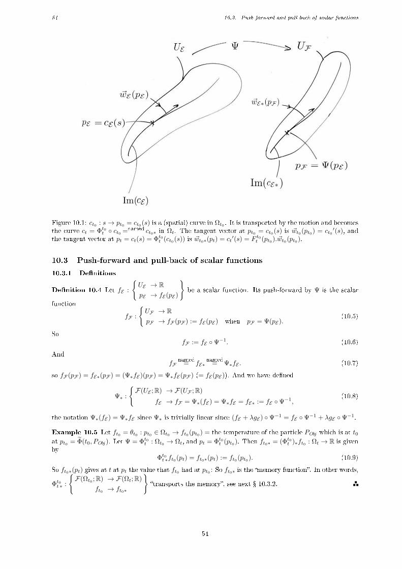
54 10.3. Push-forward and pull-back of scalar functions
Figure 10.1: ct0 : s→ pt0 = ct0(s) is a (spatial) curve in Ωt0 . It is transported by the motion and becomesthe curve ct = Φt0t ct0 =named ct0∗ in Ωt. The tangent vector at pt0 = ct0(s) is ~wt0(pt0) = ct0
′(s), andthe tangent vector at pt = ct(s) = Φt0t (ct0(s)) is ~wt0∗(pt) = ct
′(s) = F t0t (pt0). ~wt0(pt0).
10.3 Push-forward and pull-back of scalar functions
10.3.1 Denitions
Denition 10.4 Let fE :
UE → RpE → fE(pE)
be a scalar function. Its push-forward by Ψ is the scalar
function
fF :
UF → RpF → fF (pF ) := fE(pE) when pF = Ψ(pE).
(10.5)
SofF := fE Ψ−1. (10.6)
And
fFnamed
= fE∗named
= Ψ∗fE . (10.7)
so fF (pF ) = fE∗(pF ) = (Ψ∗fE)(pF ) = Ψ∗fE(pF ) (= fE(pE)). And we have dened
Ψ∗ :
F(UE ;R) → F(UF ;R)
fE → fF = Ψ∗(fE) = Ψ∗fE = fE∗ := fE Ψ−1,(10.8)
the notation Ψ∗(fE) = Ψ∗fE since Ψ∗ is trivially linear since (fE + λgE) Ψ−1 = fE Ψ−1 + λgE Ψ−1.
Example 10.5 Let ft0 = θt0 : pt0 ∈ Ωt0 → ft0(pt0) = the temperature of the particle PObj which is at t0at pt0 = Φ(t0, PObj ). Let Ψ = Φt0t : Ωt0 → Ωt, and pt = Φt0t (pt0). Then ft0∗ = (Φt0t )∗ft0 : Ωt → R is givenby
Φt0t ∗ft0(pt) = ft0∗(pt) := ft0(pt0). (10.9)
So ft0∗(pt) gives at t at pt the value that ft0 had at pt0 : So ft0∗ is the memory function. In other words,
Φt0t ∗ :
F(Ωt0 ;R) → F(Ωt;R)
ft0 → ft0∗
transports the memory, see next 10.3.2.
54
55 10.4. Push-forward and pull-back of curves
Denition 10.6 Let fF :
UF → RpF → fF (pF )
be a scalar function. Its pull-back by Ψ is the push-forward
by Ψ−1, i.e., is the scalar function
fEnamed
= fF∗ named
= Ψ∗fF :
UE → RpE → fF
∗(pE) := fF (pF ) when pF = Ψ(pE).(10.10)
And the pull-back fF∗ of fF by Ψ is also named Ψ∗fF , so
fF∗ = Ψ∗fF := fF Ψ, and Ψ∗fF (pE) = fF (pF ) when pF = Ψ(pE). (10.11)
Proposition 10.7Ψ∗ Ψ∗ = I and Ψ∗ Ψ∗ = I. (10.12)
Proof. Ψ∗(Ψ∗fE)(pE) = Ψ∗fE(pF ) = fE(pE), thus Ψ∗ Ψ∗ : F(UE ;R)→ F(UE ;R) is the identity.Ψ∗(Ψ
∗fF )(pF ) = Ψ∗fF (pE) = fF (pF ), thus Ψ∗ Ψ∗ : F(UF ;R)→ F(UF ;R) is the identity.
10.3.2 Interpretation: Why is it useful?
Following example 10.5. We record the temperature θ(t, p) at all t and all p. So θ :C =⋃t
(t × Ωt) → R
(t, p) → θ(t, p)
is a Eulerian scalar valued function, cf. (2.2). Then we consider its
restriction θt0 :
Ωt0 → Rpt0 → θt0(pt0) := θ(t0, pt0)
which gives the temperatures at t0 in Ωt0 . The push-
forward of the function θt0 by Φt0t is the memory function, cf. (10.5),
θt0∗ = Φt0t ∗θt0 := θt0 (Φt0t )−1 :
Ωt → Rpt → θt0∗(pt) := θt0(pt0) when pt = Φt0t (pt0).
(10.13)
Question: Why do we introduce θt0∗ since we have θt0?Answer: An observer does not have the gift of temporal and/or spatial ubiquity; He can only consider
values at the actual t at the actual pt where he is (time and space). See remark 1.3.E.g., at t0 at pt0 the observer writes the value θt0(pt0) on a piece of paper (for memory), then put
the piece of paper is his pocket; And once arrived at t at pt, he reads the value on the paper and nameit θt0∗(pt), or more explicitly Φt0t ∗θt0(pt), because he is now at t at pt, so with θt0∗(pt) := θt0(pt0).
Application: Then, at pt at t, the observer can compare the actual value θt(pt) with the transportedvalue θt0∗(pt) = the memory (no need of any ubiquity gift): Here, for scalar valued functions, we simplyget
θt(pt)− θt0∗(pt) = θt(pt)− θt0(pt0). (10.14)
With (10.14), the Lie derivative will be easy to understand.
10.4 Push-forward and pull-back of curves
With (10.1). Let
cE :
]− ε, ε[ → UE
s → pE = cE(s)(10.15)
be a curve in UE , see gure 10.1.
Denition 10.8 The push-forward of cE :]− ε, ε[→ UE by Ψ is the curve
cF := ΨcEnamed
= cE∗named
= Ψ∗cE :
]− ε, ε[ → UF
s → cF (s) = cE∗(s) := Ψ(cE(s)) (= Ψ(pE) = pF ),(10.16)
so Im(cF ) = Ψ(cE), that is, Im(cF ) is made of the push-fowards of the points of Im(cE), see gure 10.1.
55
56 10.5. Push-forward and pull-back of vector elds
Example 10.9 See gure 10.1. Ψ = Φt0t , and cE = ct0 :
]− ε, ε[ → Ωt0
s → pt0 = ct0(s).
(so s is a space
variable). And
ct = ct0∗ = Φt0t ct0 :
]− ε, ε[ → Ωt
s → pt = ct(s) := Φt0t (pt0) when pt = Φt0t (pt0) = pt0∗.(10.17)
And Im(ct0∗) = Φt0t (Im(ct0)).
Denition 10.10 If
cF :
]− ε, ε[ → UF
s → pF = cF (s)(10.18)
is a curve in UF then its pull-back cE = cF∗ by Ψ is its push-forward by Ψ−1:
cE = cF∗ := Ψ−1 cF :
]− ε, ε[ → UE
s → pE = cE(s) = cF∗(s) := Ψ−1(cF (s)) = Ψ−1(pF ).
(10.19)
10.5 Push-forward and pull-back of vector elds
This is one of the most important concept for mechanical engineers. We need a norm ||.||E in E (we needrst-order Taylor expansions).
10.5.1 Approximate description: Transport of a small bipoint vector
Let pE and qE be points in UE , and let pF = pE∗ = Ψ(pE) and qF = qE∗ = Ψ(qE) in UF be thepush-forwards by Ψ cf. (10.1). The rst order Taylor expansion gives
(Ψ(qE)−Ψ(pE) =) qF − pF = dΨ(pE).(qE − pE) + o(||qE − pE ||E), (10.20)
that is,−−−→pFqF = dΨ(pE).−−→pEqE + o(||−−→pEqE ||E). (10.21)
By neglecting the o(||−−→pEqE ||E) we get:
Denition 10.11 Let ~wE(pE) ∈ E be a vector at pE ∈ U ; Its push-forward by Ψ is the vector~wF (pF ) =named ~wE∗(pF ) =named Ψ∗ ~wE(pF ) ∈ F dened at pF = pE∗ = Ψ(pE) ∈ UF by
Ψ∗ ~wE(pF ) = ~wE∗(pF ) := dΨ(pE). ~wE(pE)noted
= Ψ∗ ~wE(pF ). (10.22)
This denition obtained with (10.21) is not really satisfactory for an unambiguous use in classicalmechanics (the bad understanding is made obvious at 5.2). A satisfactory approach consists in rewrit-ing (10.20) with qE = pE + h~wE (with h small, e.g., h ' ||qE − pE ||E and ||~wE ||E ' 1) as
Ψ(pE + h~wE)−Ψ(pE) = h dΨ(pE). ~wE + o(h), (10.23)
thus, for all ~wE ∈ E (whatever its length, in particular for all ~wE s.t. ||~wE ||E = 1), Ψ(pE+h~wE)−Ψ(pE)h =
dΨ(pE). ~wE + o(1) as h→ 0. We recover the denition of the dierential of Ψ at pE in any direction ~wE :
dΨ(pE). ~wE = limh→0
Ψ(pE + h~wE)−Ψ(pE)
h
named= ~wE∗(pF ) at pF = Ψ(pE). (10.24)
(Recall: The dierential dΨ(pE) : E → F is linear.)
Quantication (with components): Let (~ai) and (~bi) be bases in E and F . Then (10.24) gives
[~wE∗(pF )]|~b = [dΨ(pE)]|~a,~b.[~wE(pE)]|~a. (10.25)
56
57 10.5. Push-forward and pull-back of vector elds
10.5.2 Denition of the push-forward of a vector eld
To fully grasp the denition 10.11, cf. (10.22) or (10.24), we use an unambiguous denition of a vectoreld: A function made of tangent vectors to a curve (this approach gives the push-forward on anymanifold, e.g., on any non-planar surface considered alone, that is, as not immersed in an ane space).So, cf. gure 10.1:
• Let cE be a regular curve in UE , cf. (10.15). The tangent vector at Im(cE) at pE = cE(s) is
~wE(pE) := ~cE′(s) (= lim
h→0
cE(s+ h)− cE(s)h
∈ E). (10.26)
See gure 10.1. This denes the vector eld ~wE :
Im(cE) → E
pE → ~wE(pE)
in Im(cE) ⊂ UE .
• The push-forward curve by Ψ is cE∗ = Ψ cE , cf. (10.16) (the curve transformed by Ψ). Thus thetangent vector at Im(cE∗) at pF = cE∗(s) is
(Ψ∗ ~wE)(pF ) = ~wE∗(pF ) := cE∗′(s) (= lim
h→0
cE∗(s+ h)− cE∗(s)h
∈ F ). (10.27)
See gure 10.1. This denes the vector eld ~wE∗ :
Im(cE∗) → F
pF → ~wE∗(pF )
in Im(cE∗) ⊂ UF .
• And cE∗ = Ψ cE gives cF∗′(s) = dΨ(cE(s)). ~cE′(s) for all s ∈]− ε, ε[, thus
(Ψ∗ ~wE)(pF ) = ~wE∗(pF ) = dΨ(pE). ~wE(pE) when pF = Ψ(pE). (10.28)
• In particular, with rectilinear curves, we recover (10.24) (denition of the dierential).
Denition 10.12 Let ~wE :
UE → E
pE → ~wE(pE)
be a regular vector eld in UE (so it has integral curves cE).
Its push-forward by Ψ is the vector eld Ψ∗ ~wE = ~wE∗ :
UF → F
pF → Ψ∗ ~wE(pF ) = ~wE∗(pF )
dened
by (10.28) (its integral curves are the cE∗ = Ψ cE). That is,
Ψ∗ ~wE = ~wE∗ := (dΨ. ~wE) Ψ−1, (10.29)
the notation ~wE∗ being used if Ψ is implicit.
This denes the map Ψ∗ :
F(UE ;E) → F(UF ;F )
~wE → Ψ∗(~wE) := Ψ∗ ~wE = ~wE∗
. (We use the same notation Ψ∗
as in denition 10.4 for scalar valued functions: The context removes ambiguity.)
10.5.3 Interpretation: Essential to continuum mechanics
Continuing example 10.9, see gure 10.1.
Consider a Eulerian vector valued function ~w :
C =⋃t
(t × Ωt) → ~Rn
(t, p) → ~w(t, p)
, cf. (2.2), e.g. a force
eld. Then, at t0 consider ~wt0 :
Ωt0 → ~Rnt0pt0 → ~wt0(pt0) := ~w(t0, pt0)
(the force eld at t0). And (10.28)
reads
~wt0∗(pt) = F t0t (pt0). ~wt0(pt0) = the push-forward of ~wt0(pt0) by Φt0t , (10.30)
see gure 10.1, with ~wt0∗(pt) ∈ ~Rnt .Application: At pt at t, the observer can compare the actual value ~wt(pt) (e.g. the actual force) withthe transported value ~wt0∗(pt) = (Ψ∗ ~wt0)(pt) ( = the transported memory see next remark 10.13 = thevector that has let itself be deformed by the ow): The dierence
~wt(pt)− ~wt0∗(pt) is meaningful at t at pt for one observer (10.31)
without any ubiquity gift (time or space). This dierence gives a measure of the stress, and the rate
limt→t0~wt(pt)−~wt0∗(pt)
h denes the Lie derivative, see 15.5.
57
58 10.6. Quantication with bases
Remark 10.13 Unlike scalar functions, cf. 10.3.2: At t0 at pt0 you can't just draw a vector ~wt0(pt0)on a piece of paper, put the paper in your pocket, then let yourself be carried by the ow Ψ = Φt0t(push-forward), then, once arrived at t at pt, take the paper out of your pocket at t at pt and read it: Thedirection and the length of the vector have been modied by the ow, see (10.30) and gure 10.1: ~wt0∗(pt)is result of the deformation of ~wt0 by the ow. (A vector is not just a collection of scalar components.)(See prop. 4.10.)
Exercice 10.14 Prove:~cE′′(s) = d~wE(pE). ~wE(pE), (10.32)
andd~wE∗(pF ).dΨ(pE) = dΨ(pE).d~wE(pE) + d2Ψ(pE). ~wE(pE), (10.33)
andcE∗′′(s) = d~wE∗(pF ). ~wE∗(pF ) (= dΨ(pE). ~cE
′′(s) + d2Ψ(pE). ~cE′(s). ~cE
′(s)). (10.34)
Answer. ~cE′(s) = ~wE(cE(s)) gives ~cE
′′(s) = d~wE(cE(s)). ~cE′(s), hence (10.32).
~wE∗(Ψ(pE)) = dΦ(pE). ~wE(pE) by denition of ~wE∗, hence (10.33).
cF (s) = Ψ(cE(s)) gives ~cF′(s) = dΨ(cE(s)). ~cE
′(s) = dΨ(cE(s)). ~wE(cE(s)) = ~wE∗(cF (s)). Thus ~cF′′(s) =
(d2Ψ(cE(s)). ~cE′(s)). ~cE
′(s) + dΨ(cE(s)). ~cE′′(s) = d~wE∗(cF (s)). ~cF
′(s), hence (10.34).
10.5.4 Pull-back of a vector eld
Denition 10.15 The pull-back is the push-forward by Ψ−1. So: Let ~wF :
UF → F
pF → ~wF (pF )
be a
vector eld on UF . Its pull-back by Ψ is the vector eld ~wF∗=named Ψ∗ ~wF dened on UE by
Ψ∗ ~wF = ~wF∗ :
UE → E
pE → ~wF∗(pE) := dΨ−1(pF ). ~wF (pF ), when pF = Ψ(pE).
(10.35)
In other words,Ψ∗ ~wF = ~wF
∗ := (dΨ−1. ~wF ) Ψ. (10.36)
Proposition 10.16Ψ∗ Ψ∗ = I and Ψ∗ Ψ∗ = I, (10.37)
that is, Ψ∗(Ψ∗ ~wE) = ~wE or Ψ∗ ~wE = (Ψ∗)−1(~wE), and Ψ∗(Ψ∗ ~wE) = ~wE or Ψ∗ ~wE = (Ψ∗)
−1(~wE).
Proof. Ψ∗(Ψ∗ ~wE)(pE) = dΨ−1(pF ).Ψ∗ ~wE(pF ) = dΨ−1(pF ).dΨ(pE). ~wE(pE) = ~wE(pE), thus Ψ∗ Ψ∗ :F(UE ;E) → F(UE ;E) is the identity. Idem for the second equality. (Pull-back = inverse of push-forward).
10.6 Quantication with bases
The presentation of push-forwards were, up,to now, qualitative (observer independent). Now we quantify
(observer dependent). Let OF be a origin in F and (~bi) be a Cartesian basis in F . Let pE ∈ UE , let
pF = Ψ(pE) = OF +−−−−−−→OFΨ(pE) =
n∑i=1
ψi(pE)~bi, i.e. [−−−→OFpF ]|~b =
ψ1(pE)...
ψn(pE)
. (10.38)
Thus,
dΨ(pE) =
n∑i=1
~bi ⊗ dψi(pE), (10.39)
Thus, with the generic notation
∂f
∂xj(pE) := df(pE).~aj (= lim
h→0
f(pE + ~aj)− f(pE)
h), (10.40)
58
59 10.6. Quantication with bases
we get, for all j ∈ [1, n]N,
dΨ(pE).~aj =
n∑i=1
(dψi(pE).~aj)~bi =
n∑i=1
∂ψi
∂xj(pE)~bi, and [dΨ(pE)]|~a,~b = [
∂ψi
∂xj(pE)], (10.41)
[dΨ(pE)]|~a,~b being the Jacobian matrix of Ψ at pE relative to the chosen bases. Thus, for any vector
~wE(pE) ∈ E at pE , its push-forward is, with pF = Ψ(pE),
~wE∗(pF ) = dΨ(pE). ~wE(pE) =
n∑i=1
(dψi(pE). ~wE(pE))~bi, [~wE∗(pF )]|~b = [dΨ(pE)]|~a,~b.[~wE(pE)]|~a. (10.42)
(With tensorial expression that shows the bases is use, dΨ(pE) =∑ni=1
∂ψi
∂xj (pE)~bi ⊗ aj , where (ai) is thedual basis of (~ai).)
Example 10.17 Change of coordinate system interpreted as a push-forward: Paradigmatic exampleof the polar coordinate system. Consider the Cartesian vector space R × R=named ~R2
p = ~q = (r, θ)(parametric space), with its canonical basis ( ~A1, ~A2), and ~q = r ~A1 + θ ~A2 =named(r, θ). And considerthe geometric ane space R2 (of positions) with a point O (origin), together with its associated vector
space ~R2 and with a Euclidean basis ( ~E1, ~E2). Then consider the polar coordinate system, that is, themap
Ψ :
~R2p−~0 = (R× R)−~0 → R2
~q = (r, θ) → p = p(~q) = Ψ(~q) = Ψ(r, θ), and−→Op
named= ~x,
(10.43)
where −→Op = ~x = Ψ1(r, θ) ~E1 + Ψ2(r, θ) ~E2 = r cos θ ~E1 + r sin θ ~E2, (10.44)
i.e.,
[~x]|~E = [−−−−→OΨ(~q)]|~E =
(Ψ1(r, θ) = x = r cos θΨ2(r, θ) = y = r sin θ
). (10.45)
The need to use p instead of ~x appears when a surface in R3 is considered.The i-th coordinate line at ~q = (r, θ) in the parametric space ~R2
p is the straight line ~c~q,i : s ∈ R →~c~q,i(s) = ~q + s ~Ai, so with ~c~q,i(0) = ~q, and its tangent vector at ~c~q,i(s) is ~c~q,i
′(s) = ~Ai (independent of s:Cartesian basis).
This line is transformed by Ψ into the polar coordinate line at p which is the curve cp,i = Ψ ~c~q,i :
s ∈ R → cp,i(s) = Ψ(~q + s ~Ai), so cp,i(0) = p and [cp,1(s)]|~E =
((r+s) cos θ(r+s) sin θ
)(straight line) and
[cp,1(s)]|~E =
(r cos(θ+s)r sin(θ+s)
)(circle). And the tangent vector at cp,i(s) is cp,i
′(s) =named ~ai∗(p), thus, with
−→Op = Ψ(~q) = Ψ(r, θ),
~a1∗(p) = dΨ(~q). ~A1 = limh→0
Ψ(~q+ ~A1)−Ψ(~q)
h=∂Ψ
∂r(~q), and [~a1∗(p)]|~E =
(cos θsin θ
),
~a2∗(p) = dΨ(~q). ~A2 = limh→0
Ψ(~q+ ~A2)−Ψ(~q)
h=∂Ψ
∂θ(~q), and [~a2∗(p)]|~E =
(−r sin θr cos θ
).
(10.46)
The basis (~a1∗(p),~a2∗(p)) is the polar coordinate system basis at p. In other words, the Jacobian matrix
of Ψ at ~q is [dΨ(~q)]| ~A, ~E =(
[~a1∗(p)]|~E [~a2∗(p)]|~E)
=(
[∂Ψ∂r (~q)]|~E [∂Ψ
∂θ (~q)]|~E)
=
(cos θ −r sin θsin θ r cos θ
)=
[∂Ψi
∂qj (~q)] when p = Ψ(~q).
Toward derivation: The Christoel symbols γkij(p) ∈ R at p are the components of d~aj∗(p).~ai∗(p) inthe coordinate basis (~ak∗(p)):
d~aj∗(p).~ai∗(p) =
n∑k=1
γkij(p)~ak∗(p). (10.47)
And ~aj∗(p) = dΨ(~q). ~Aj at p = Ψ(~q) gives (~aj∗ Ψ)(~q) = dΨ(~q). ~Aj , thus d~aj∗(p).dΨ(~q). ~Ai =
59
60 10.6. Quantication with bases
d2Ψ(~q)( ~Ai, ~Aj), thus
d~aj∗(p).~ai∗(p) =∂2Ψ
∂qi∂qj(~q), (10.48)
thus Ψ C2 gives γkij(p) = γkji(p) for all i, j, k (symmetry of the bottom indices for a holonomous basis =the basis of a coordinate system).
For the polar coordinates, ∂Ψ∂r (~q) = cos θ ~E1 + sin θ ~E2 gives ∂2Ψ
∂r2 (~q) = 0, thus γ111 = γ2
11 = 0, and∂2Ψ∂θ∂r (~q) = − sin θ ~E1 + cos θ ~E2 = 1
r~a2∗(p), thus γ112 = 0 and γ2
12 = 1r . And
∂Ψ∂θ (~q) = −r sin θ ~E1 + r cos θ ~E2
gives ∂2Ψ∂θ2 (~q) = −r cos θ ~E1 − r sin θ ~E2 = −r~a1∗(p), thus γ
122 = −r and γ2
22 = 0.Application with f a C2(Rn;R) function, when f(p) = g(~q) at p = Ψ(~q), that is, when f is given by
(f Ψ)(~q) =named g(~q). Then ∂f∂xi (p) = df(p). ~Ei is the usual notation, as well as
∂g∂qi (~q) = dg(~q). ~Ai; Then
by denition ∂f∂qi (p) := ∂g
∂qi (~q) (recall f is a function of p, not a function of ~q, so this is the denition).Thus,
∂f
∂qi(p) = dg(~q). ~Ai = df(Ψ(~q)).dΨ(~q). ~Ai = df(p).~ai∗(p) = (df.~ai∗)(p). (10.49)
Thus for second order derivation, with (df.~ai∗)(p) = (df.~ai∗)(Ψ(~q)) we get
∂ ∂f∂qi
∂qj(p) = d(df.~ai∗)(p).~aj∗(p) = d((df(p).~aj∗(p)).~ai∗(p) + df(p).(d~ai∗(p).~aj(p)), (10.50)
thus∂2f
∂qi∂qj(p) = d2f(p)(~ai∗(p),~aj∗(p) +
n∑k=1
∂f
∂xk(p)γkij(p)~ak(p). (10.51)
So rst order derivatives for f are still alive: The Christoel symbols have appeared.NB: The independent variables r and θ don't have the same dimension (a length and an angle): There
is no physical meaningful inner dot product in the parameter space ~R2p = R×R = (r, θ), but this space
is however very useful! (As in thermodynamics: No inner dot product in the (T, V ) space.)NB: ~ai∗(p) is also noted ~ai∗(~x): Here we are in the at geometric space R2, and a point p can be
spotted thanks to a bi-point vector ~x =−→Op.
NB: The normalized basis (~a1∗(p),1r~a2∗(p)) is not holonomic, that is, is not the basis of a coordinate
system, and its use makes derivations quite complicated (no symmetry for the Christoel symbols).
11 Homogeneous and isotropic material
Framework: linear modelization and elastic materials.Let P ∈ Ωt0 , and suppose that the Cauchy stress vector ~ft(pt) à t at pt = Φt0t (P ) only depends on
P and on F t0t (P ) = dΦt0t (P ) = the dierential of the motion, or rst (covariant) gradient, that is,
~ft(pt) = ~function(P, F t0t (P )). (11.1)
Denition 11.1 A material is homogeneous i ~function doesn't depend on the rst variable P , i.e., i,for all P ∈ Ωt0 ,
(~ft(pt) =) ~function(P, F t0t (P )) = ~function(F t0t (P )). (11.2)
Denition 11.2 (Isotropy.) Consider an inner dot product, the same at any time. A material is isotropic
at a point P ∈ Ωt0 i ~function doesn't depend on the direction you consider, i.e., i, for any rotationRt0(P ),
(~ft(pt) =) ~function(P, F t0t (P )) = ~function(P, F t0t (P ).Rt0(P )). (11.3)
Denition 11.3 A material is isotropic homogeneous i, for all P ∈ Ωt0 and for all rotation Rt0(P ):
(~ft(pt) =) ~function(P, F t0t (P ).Rt0(P )) = ~function(F t0t (P )). (11.4)
60
61 12.1. Denition of H = F−1
12 The inverse of the deformation gradient
12.1 Denition of H = F−1
Let t0, t ∈ R, Φt0t :
Ωt0 → Ωt
P → p = Φt0t (P )
, and F t0t = dΦt0t :
~Rnt0 → ~Rnt
~W (P ) → ~w(p) = F t0t (P ). ~W (P )
. With
p = Φt0t (P ) and ((Φt0t )−1 Φt0t )(P ) = P we get
d(Φt0t )−1(p).dΦt0t (P ) = It0 , thus d(Φt0t )−1(p) = dΦ(P )−1. (12.1)
Thus
(F t0t )−1(p) := F t0t (P )−1
~Rnt → ~Rnt0
~w(p) → ~W (P ) = (F t0t )−1(p). ~w(p) := F t0t (P )−1. ~w(p).(12.2)
Thus, we have dened
Ht0t := (F t0t )−1 :
Ωt → L(~Rnt ; ~Rnt0)
p → Ht0t (p) := (F t0t )(P )−1 = F t0t
−1(p) when p = Φt0t (P ).
(12.3)
(And Ht0t is a two point tensor.)
Then let
Ht0 :
C =⋃t
(t × Ωt) → L(~Rnt ; ~Rnt0)
(t, pt) → Ht0(t, pt) := Ht0t (pt) (= (F t0(t, P ))−1 when pt = Φt0(t, P )).
(12.4)
NB: Ht0 looks like a Eulerian map, but isn't: Ht0 depends on a initial time t0. We will however use thematerial time derivative D
Dt notation in this case, that is we dene, along a trajectory t→ p(t) = Φt0(t, P ),
DHt0
Dt(t, p(t)) :=
∂Ht0
∂t(t, p(t)) + dHt0(t, p(t)).~v(t, p(t)), written
DHt0
Dt=∂Ht0
∂t+ dHt0 .~v, (12.5)
time derivative g′(t) of the function g : t→ g(t) = Ht0(t,Φt0(t, P )) = Ht0(t, Φ(t, PObj )).
Exercice 12.1 Prove that DHt0
Dt (t, p(t)) = Ht0t1 (pt1).DH
t1
Dt (t, p(t)).
Answer. (6.18) gives p(t) = Φt0t (pt0) = Φt1t (Φt0t1(pt0)), and let pt1 = Φt0t1(pt0).
Hence F t0t (pt0) = F t1t (pt1).F t0t1 (pt0), thus F t0t (pt0)−1 = F t0t1 (pt0)−1.F t1t (pt1)−1, thus Ht0t (p(t)) =
Ht0t1
(pt1).Ht1t (p(t)), that is, Ht0(t, p(t)) = Ht0
t1(pt1).Ht1(t, p(t)). Thus the result.
12.2 Time derivatives of H
Let p(t) = Φt0(t, P ). Since Ht0(t, p(t)).F t0(t, P ) = It0 , we get, with the shortened notation H.F = I,
DH
Dt.F +H.
∂F
∂t= 0, and
D2H
Dt2.F + 2
DH
Dt.∂F
∂t+H.
∂2F
∂t2= 0. (12.6)
(Full notations: DHt0
Dt (t, p(t)).F t0(t, P ) +Ht0(t, p(t)).∂Ft0
∂t (t, P ) = 0, andD2Ht0
Dt2 (t, p(t)).F t0(t, P ) + 2DHt0
Dt (t, p(t)).∂Ft0
∂t (t, P ) +Ht0(t, p(t)).∂2F t0
∂t2 (t, P ) = 0.)Thus, with (5.39),
DH
Dt= −H.∂F
∂t.F−1 = −H.d~v, (12.7)
thus, with (5.43) :
D2H
Dt2= −(
DH
Dt).d~v −H.D~v
Dt= H.d~v.d~v −H.d~γ = −H.D(d~v)
Dt. (12.8)
So the second order Taylor expansion in time (along a trajectory) is
Ht0(t+h, p(t+h)) = Ht0(I − h d~v − h2
2
D(d~v)
Dt(t, p(t)) + o(h2)
= Ht0(I − h d~v − h2
2(d~γ − d~v.d~v))(t, p(t)) + o(h2).
(12.9)
In particular:
Ht0(t0+h, p(t0+h)) = (I − h d~v − h2
2(d~γ − d~v.d~v))(t0, pt0) + o(h2). (12.10)
61
62 13.1. Denition
Exercice 12.2 Check that (12.9) and (5.41) give F−1.F = I, up to the second order.
Answer.
F t0P (t+h)−1.F t0P (t+h) = [F−1.(I − h d~v − h2
2(d~γ − d~v.d~v)) + o(h2)].[
(I + h d~v +
h2
2d~γ).F + o(h2)]
= F−1.(I + h (d~v − d~v) +h2
2(d~γ − d~v.d~v − (d~γ − d~v.d~v)) + o(h2)).F = I + o(h2).
Exercice 12.3 Prove (12.7), using the derivation of Ht0(t, p(t)). ~wt0∗(t, p(t)) = ~W (P ) when p(t) =
Φt0(t, P ) and ~wt0∗(t, p(t)) = F t0(t, P ). ~W (P ).
Answer. DHt0
Dt. ~wt0t∗ + Ht0 .
D~wt0t∗
Dt= 0, and
D~wt0t∗
Dt(t, p(t)) = ∂F t0
∂t(t, P ). ~W (P ) = d~v(t, p(t)).F t0(t, P ). ~W (P ) =
d~v(t, p(t)). ~wt0t∗(t, p(t)), thusDHt0
Dt. ~wt0t∗ +Ht0 .d~v.~wt0t∗ = 0, thus DH
Dt= −H.d~v.
13 Push-forward and pull-back of dierential forms
13.1 Denition
Setting of 10.1: UE is an open set in the ane space E associated to the normed vector space E.
Let αE :
UE → E∗ = L(E;R)
pE → αE(pE)
be a dierential form on UE (a eld of linear forms), that is
αE ∈ Ω1(UE) = T 01 (UE), cf. (R.11). If ~wE :
UE → E
pE → ~wE(pE)
∈ Γ(UE) (a eld of vectors in UE) then
fE = αE . ~wE :
UE → RpE → fE(pE) = (α.~wE)(pE) = αE(pE). ~wE(pE)
is a scalar function which gives the value of αE on ~wE (a eld of scalar functions which gives the measureof ~wE by αE).
Consider a dieomorphism Ψ, cf. (10.1). The push-forward of fE = αE . ~wE by Ψ is fE∗ = Ψ∗(fE) =Ψ∗(αE . ~wE), and is given by, with pF = Ψ(pE), cf. (10.5) ,
Ψ∗(αE . ~wE)(pF ) = (αE . ~wE)(pE) = αE(pE). ~wE(pE). (13.1)
Since the push-forward of a vector eld ~wE is given by ~wE∗(pF ) = dΨ(pE). ~wE(pE), cf. (10.28), we get
Ψ∗(αE . ~wE)(pF ) = αE(pE).dΨ(pE)−1︸ ︷︷ ︸
αE∗(pF )
. ~wE∗(pF ), (13.2)
so (compatibility hypothesis):
Denition 13.1 Let αE ∈ Ω1(UE) a dierential form (a regular eld of linear forms on UE). Its push-forward by Ψ is the dierential form αE∗ ∈ Ω1(UF ) dened by, with pF = Ψ(pE),
αE∗(pF ) := αE(pE).dΨ(pE)−1 named
= (Ψ∗αE)(pF ). (13.3)
In other words,αE∗ := (αE Ψ−1).dΨ−1 (= Ψ∗αE). (13.4)
(See also remark 13.6.)
Proposition 13.2 For all αE ∈ Ω1(UE), all αF ∈ Ω1(UF ), all ~wF ∈ Γ(UF ), all ~wE ∈ Γ(UE), in short
αE∗. ~wF = αE . ~wF∗, and αF
∗. ~wE = αF . ~wE∗. (13.5)
Full notation: αE∗(pF ). ~wF (pF ) = αE(pE). ~w∗F (pE), and αF
∗(pE). ~wE(pE) = αF (pF ). ~wE∗(pF ), for all pF =Ψ(pE) ∈ UF .
62
63 13.2. Incompatibility: Riesz representation and push-forward
Proof. αE∗(pF ). ~wF (pF ) = (αE(pE).dΨ−1(pF )). ~wF (pF ) = αE(pE).(dΨ−1(pF ). ~wF (pF )) = αE(pE). ~w∗F (pE),
for all pF = Ψ(pE) ∈ UF . Idem for the second equality.
Proposition 13.3 The dierential of a scalar function commutes with the push-forward, that is, iff ∈ C1(UE ;R) then
d(Ψ∗f
)= Ψ∗
(df), (13.6)
that is, d(Ψ∗f
)(pF ) = Ψ∗
(df)(pF ) for all pF ∈ UF .
Proof. Let pF = Ψ(pE). We have Ψ∗f(pF ) = f(pE) = f(Ψ−1(pF )), cf. (10.5). Thus d(Ψ∗f)(pF ) =df(pE).dΨ−1(pF ).
And (13.3) gives (Ψ∗(df))(pF ) = df(pE).dΨ(pE)−1. With dΨ(pE)
−1 = dΨ−1(pF ) we get (13.6).
Denition 13.4 Let αF : UF → F ∗. Its pull-back by Ψ is the dierential form αF∗ = Ψ∗αF : UE → E∗
dened by, with pE = Ψ−1(pF ),
αF∗(pE) = Ψ∗αF (pE) := αF (pF ).dΨ(pE). (13.7)
In other words,αF∗ = Ψ∗αF := (αF Ψ).dΨ. (13.8)
(See also remark 13.6.)
Proposition 13.5Ψ∗ Ψ∗ = I and Ψ∗ Ψ∗ = I. (13.9)
Proof. Ψ∗(Ψ∗αE)(pE) = Ψ∗αE(pF ).dΨ(pE) = αE(pE).dΨ−1(pF ).dΨ(pE) = αE(pE).Ψ∗(Ψ
∗αF )(pF ) = Ψ∗αF (pE).dΨ−1(pF ) = αF (pF ).dΨ(pE).dΨ−1(pF ) = αF (pF ).
Remark 13.6 The pull-back Ψ∗αF can also be dened thanks to the natural canonical isomorphismL(E;F ) → L(F ∗;E∗)
L → L∗
given by L∗(`F ).~uE = `F .(L.~uE) for all ~uE ∈ E. That is, L∗(`F ) = `F .L,
and L∗(`F ) is called the pull-back of `F by L. In particular, if `F = αF (pF ) and L = dΨ(pE) thendΨ(pE)
∗(αF (pF )) = αF (pF ).dΨ(pE), that is (13.7). And this approach gives: αF∗ = Ψ∗αF is covariant
objective (independent of any observer).And, if Ψ is invertible, then the push-forward is the pull-back considered with Ψ−1 instead of Ψ.
13.2 Incompatibility: Riesz representation and push-forward
A push-forward is independent of any inner dot product. Now we quantify with inner dot products(observer dependent). Let (·, ·)g be an inner dot product in E, and let (·, ·)h be an inner dot productin F .
Let αE ∈ Ω1(UE) and αF ∈ Ω1(UF ). Thus αE(pE) ∈ E∗ for all pE ∈ UE , and αF (pF ) ∈ F ∗ for allpF ∈ UF .
Let ~αEg(pE) ∈ E be the (·, ·)g-Riesz representation vector of αE(pE), and let ~αFh(pF ) ∈ F be the(·, ·)h-Riesz representation vector of αF (pF ), that is, for all ~wE(pE) ∈ E and all ~wF (pF ) ∈ F ,
αE(pE). ~wE(pE) = (~αEg(pE), ~wE(pE))g, and αF (pF ). ~wF (pF ) = (~αFh(pF ), ~wF (pF ))h. (13.10)
This denes the vector elds ~αEg in UE and ~αFh in UF (dependent on (·, ·)g and (·, ·)h).Recall: The transposed relative to (·, ·)g and (·, ·)h of the linear map dΨ(pE) ∈ L(E;F ) is the linear
map dΨ(pE)Tgh ∈ L(F ;E) dened by
(dΨ(pE)Tgh. ~wF , ~wE)g = (~wF , dΨ(pE). ~wE)h (13.11)
for all ~wE ∈ E and ~wF ∈ F , cf. (A.24).
63
64 14.1. Push-forward and pull-back of order 1 tensors
Proposition 13.7 If αF = Ψ∗αE (= the push-forward of αE by Ψ), then
~αFh(pF ) = dΨ(pE)−Tgh .~αEg(pE), so ~αFh 6= Ψ∗~αEg in general, (13.12)
that is, ~αFh is not the push-forward of ~αEg unless dΨ(pE)−Tgh = dΨ(pE), i.e., unless dΨ(pE)
Tgh.dΨ(pE) = IE
(a rigid like body motion).So the Riesz representation vector of the push-forwarded linear form is not the push-forwarded rep-
resentation vector of the linear form push-forwarded. (This is expected: a push-forward is independentof any inner dot product, when a Riesz representation vector has no existence without an inner dotproduct.)
Proof. pF = Ψ(pE) and αF = Ψ∗αE give αF (pF ) = αE(pE).dΨ−1(pF ), cf. (13.3). And (13.10) gives
(~αFh(pF ), ~wF (pF ))h = αF (pF ). ~wF (pF ) = (αE(pE).dΨ(pE)−1). ~wF (pF ) = αE(pE).(dΨ(pE)
−1. ~wF (pF ))
= (~αEg(pE), dΨ(pE)−1. ~wF (pF ))g = (dΨ(pE)
−Tgh .~αEg(pE), ~wF (pF ))h.
(13.13)True for all ~wF , hence (13.12).
So it is better to avoid using a representation vector (not intrinsic to the dierential form) when usingpush-forwards, cf. (B.8). That is, it is better to consider the original (the dierential form) rather thana representative (a vector of representation: Which one, cf. (B.8)?).
Reminder: There is no natural canonical isomorphism between E and E∗, see T.2, and covariancecannot be confused with contravariance.
14 Push-forward and pull-back of tensors
To lighten the presentation, we deal with order 1 and 2 tensors. Similar approach for any tensor.
14.1 Push-forward and pull-back of order 1 tensors
We write (10.28) with T ' ~wE ∈ T 10 (UE) ' Γ(UE)) and (13.3) with T = α ∈ T 0
1 (UE) as, in short,
(T∗ =) Ψ∗(T ) = T (Ψ∗), (14.1)
that is, for all ξ a vector eld or a dierential form in UF when required, in short,
(Ψ∗T )(ξ) = T (Ψ∗ξ), (14.2)
that is (Ψ∗T )(pF )(ξ(pF )) = T (pE)(Ψ∗ξ(pE)) when pF = Ψ(pE). Indeed:
• If T = αE ∈ T 01 (UE) = Ω1(UE) then ξ = ~wF ∈ Γ(UF ) gives, (Ψ∗αE)(pF ) and αE(pE) being linear,
(Ψ∗αE)(pF ). ~wF (pF )(14.2)
= αE(pE).Ψ∗ ~wF (pE)
(10.35)= αE(pE).dΨ−1(pE). ~wF (pF ). (14.3)
True for all ~wF : We do get Ψ∗αE(pF ) = αE(pE).dΨ−1(pE), i.e. (13.3).• If T ∈ T 1
0 (UE), then ξ = αF ∈ Ω1(UE) gives
(Ψ∗T )(pF )(αF (pF ))(14.2)
= T (pE)(Ψ∗αF (pE))
(13.7)= T (pE)(αF (pF ).dΨ(pE)), (14.4)
and the natural canonical isomorphism J :
E → E∗∗
~w → L~w
dened by L~w(`) = `. ~w for all ` ∈ E∗,
cf. (Q.11), gives
αF (pF ).(Ψ∗ ~wE)(pF ) = Ψ∗αF (pE). ~wE(pE) = αF (pF ).dΨ(pE). ~wE(pE). (14.5)
True for all αF : We do get Ψ∗ ~wE(pF ) = dΨ(pE). ~wE(pE), i.e. (10.28).Idem for pull-backs:
(T ∗ =) Ψ∗(T ) = T (Ψ∗), (14.6)
that is (Ψ∗T )(pE)(zE(pE)) = T (pF )(Ψ∗zE(pF )) when pF = Ψ(pE).
64
65 14.2. Push-forward and pull-back of order 2 tensors
14.2 Push-forward and pull-back of order 2 tensors
Denition 14.1 Let T be an order 2 tensor on UE . Its push-forward by Ψ is the order 2 tensor on UFdened by, in short,
(T∗(·, ·) :=) Ψ∗T (·, ·) := T (Ψ∗·,Ψ∗·). (14.7)
Full notation: T∗(pF )(ξ1(pF ), ξ2(pF )) := T (pE)(ξ1∗(pE), ξ2
∗(pE)) when pF = Ψ(pE), for all ξ1, ξ2 vectorelds or dierential forms in ΩF as required.
Let T be an order 2 tensor on UF . Its pull-back by Ψ is the order 2 tensor on UE dened by,
(T ∗(·, ·) :=) Ψ∗T (·, ·) := T (Ψ∗·,Ψ∗·). (14.8)
Full notation: T ∗(pE)(ξ1(pE), ξ2(pE)) := T (pF )(ξ1∗(pF ), ξ2∗(pF )) when pF = Ψ(pE), for all ξ1, ξ2 vectorelds or dierential forms in ΩE as required.
(Denitions generalized to any r s tensors.)
Example 14.2 For an elementary tensor T = α1 ⊗ α2 ∈ T 02 (UE), made of dierential forms α1, α2 ∈
Ω1(UE): For all ~w1, ~w2 ∈ Γ(UF ), in short,
(α1 ⊗ α2)∗(~w1, ~w2)(14.7)
= (α1 ⊗ α2)(~w∗1 , ~w∗2)
(A.46)= (α1. ~w
∗1)(α2. ~w
∗2)
(13.5)= (α1∗. ~w1)(α2∗. ~w2), (14.9)
thus(α1 ⊗ α2)∗ = α1∗ ⊗ α2∗. (14.10)
(And any tensor is a nite sum of elementary tensors.)More generally, if T ∈ T 0
2 (UE) (e.g., a metric) then for all vector elds ~w1, ~w2 in UF , in short,
T∗(~w1, ~w2)(14.7)
= T (~w1∗, ~w2
∗) = T (dΨ−1. ~w1, dΨ−1. ~w2). (14.11)
Full notation: T∗(pF )(~w1(pF ), ~w2(pF )) = T (pE)(dΨ−1(pF ). ~w1(pF ), dΨ−1(pF ). ~w2(pF )) when pF = Ψ(pE).
Expression with bases (~ai) in E and (~bi) in F , in short: T∗(~w1, ~w2) = [~w1]T|~b.[T∗]|~b.[~w2]|~b and
T∗(~w1, ~w2) = T (~w1∗, ~w2
∗) = [~w∗1 ]T|~a.[T ]|~a.[~w∗2 ]|~a = ([~w1]T
|~b.[dΨ]−T
|~a,~b).[T ]|~a.([dΨ]−1
|~a,~b.[~w2]|~b), thus, in short,
[T∗]|~b = [dΨ]−T|~a,~b
.[T ]|~a.[dΨ]−1
|~a,~b. (14.12)
Full notation: [(Ψ∗T )(pF )]|~b = [dΨ(pE)]−T|~a,~b
.[T (pE)]|~a.[dΨ(pE)]−1
|~a,~bwhen pF = Ψ(pE).
And for the pull-back: For all vector elds ~w1, ~w2 in UE ,
T ∗(~w1, ~w2)(14.7)
= T (~w1∗, ~w2∗) = T (dΨ. ~w1, dΨ. ~w2). (14.13)
Example 14.3 For the elementary tensor T = ~u⊗ α ∈ T 11 (UE), made of the vector eld ~u ∈ Γ(UE) and
of the dierential form α ∈ Ω1(UE): For all β, ~w ∈ Ω1(UF )× Γ(UF ), in short,
(~u⊗ α)∗(β, ~w)(14.7)
= (~u⊗ α)(β∗, ~w∗)(A.46)
= (~u.β∗)(α.~w∗)(13.5)
= (~u∗.β)(α∗. ~w)(A.46)
= (~u∗ ⊗ α∗)(β, ~w), (14.14)
thus(~u⊗ α)∗ = ~u∗ ⊗ α∗. (14.15)
More generally, if T ∈ T 11 (UE) then for all vector elds ~w ∈ Γ(UF ) and dierential forms β ∈ Ω1(UF ),
T∗(β, ~w) = T (β∗, ~w∗) = T (β.dΨ, dΨ−1. ~w). (14.16)
Full notation: With pF = Ψ(pE), T∗(pF )(β(pF ), ~w(pF )) = T (pE)(β(pF ).dΨ(pE), dΨ−1(pF ). ~w(pF )).
Expression with bases (~ai) in E and (~bi) in F , in short: T∗(β, ~w) = [β]|~b.[T∗]|~b.[~w]|~b and T∗(β, ~w) =
T (β∗, ~w∗) = [β∗]|~a.[T ]|~a.[~w∗]|~a = ([β]|~b.[dΨ]|~a,~b).[T ]|~a.([dΨ]−1
|~a,~b.[~w]|~b), thus
[T∗]|~b = [dΨ]|~a,~b.[T ]|~a.[dΨ]−1
|~a,~b. (14.17)
Full notation: [(Ψ∗T )(pF )]|~b = [dΨ(pE)]|~a,~b.[T (pE)]|~a.[dΨ(pE)]−1
|~a,~bwhen pF = Ψ(pE).
65
66 14.3. Push-forward and pull-back of endomorphisms
14.3 Push-forward and pull-back of endomorphisms
Consider the natural canonical isomorphism, cf. (Q.44),
J2 :
L(E;E) → L(E∗, E;R)
L → TL = J2(L) where TL(α, ~u) := α.L.~u, ∀(α, ~u) ∈ E∗ × E.(14.18)
Denition 14.4 The push-forward by Ψ of a eld of endomorphisms L on UE is the eld of endomor-phisms Ψ∗L = L∗ on UF dened by
Ψ∗L = L∗ := (J2)−1((TL)∗), (14.19)
So, in short,
Ψ∗L = L∗ = dΨ.L.dΨ−1 . (14.20)
Full notation: L∗(pF ) = dΨ(pE).L(pE).dΨ−1(pF ) when pF = Ψ(pE). Indeed, for all (β, ~w) ∈ Ω1(UF ) ×Γ(UF ),
(TL)∗(β, ~w)(14.16)
= TL(β.dΨ, dΨ−1. ~w)(14.18)
= (β.dΨ).L.(dΨ−1). ~w = β. dΨ.L.dΨ−1︸ ︷︷ ︸=Ψ∗L
. ~w. (14.21)
And with bases we get [L∗]|~b = [dΨ]|~a,~b.[L]|~a.[dΨ]−1
|~a,~bas in (14.17).
Example 14.5 Elementary eld of endomorphisms L = (J2)−1(~u ⊗ α), i.e. L.~a = (α.~a)~u for all ~a ∈Γ(UE). Thus L∗ = (J2)−1((~u⊗ α)∗)
(14.15)= (J2)−1(~u∗ ⊗ α∗), and L∗.~b = (α∗.~b)~u∗ for all ~b ∈ Γ(UF ).
Denition 14.6 Let L be a eld of endomorphisms on UF . Its pull-back by Ψ is the eld of endomor-phisms Ψ∗L = L∗ on UE dened by, in short
Ψ∗L = L∗ = dΨ−1.L.dΨ . (14.22)
Full notation: L∗(pE) = dΨ−1(pF ).L(pF ).dΨ(pE) when pF = Ψ(pE).
14.4 Application to derivatives of vector elds
Let ~w ∈ Γ(UE) be a vector eld on UE . Its derivative d~w is a eld of endomorphisms on E, cf. example R.8.So its push-forward Ψ∗(d~w) =noted(d~w)∗ is given by, in short cf. (14.20),
(d~w)∗ = dΨ.d~w.dΨ−1. (14.23)
Full notation: (d~w)∗(pF ) = dΨ(pE).d~w(pE).dΨ(pE)−1 when pF = Ψ(pE).
14.5 Application to derivative of dierential forms
The map
J :
L(E;E∗) → L(E,E;R)
L → J(L), J(L)(~u1, ~u2) := (L.~u1).~u2,(14.24)
is a natural canonical isomorphism. Thus we can identify L with J(L). So, if T ∈ T 02 (UE) then its
push-forward Ψ∗T being given by (14.11):
Denition 14.7 Let L : UE → L(E;E∗) (a eld of linear maps). Its push-forward by Ψ is the eld oflinear maps Ψ∗L = L∗ : UF → L(F ;F ∗) given by, in short,
L∗(.) = (L.dΨ−1.(.)).dΨ−1. (14.25)
Full notation: L∗(pF ).(.) = (L(pE).dΨ−1(pF ).(.)).dΨ−1(pF ) when pF = Ψ(pE). That is, in short, for all~w ∈ T 1
0 (UF ),L∗. ~w = (L.dΨ−1. ~w).dΨ−1 ∈ F ∗. (14.26)
Full notation: L∗(pF ). ~w(pF ) = (L(pE).dΨ−1(pF ). ~w(pF )).dΨ−1(pF ) ∈ F ∗. That is, in short, for all~w1, ~w2 ∈ Γ(UF ),
(L∗. ~w1). ~w2 = (L.dΨ−1. ~w1).dΨ−1. ~w2 ∈ R, (14.27)
cf. (14.11). Full notation: (L∗(pF ). ~w1(pF )). ~w2(pF ) = (L(pE).dΨ−1(pF ). ~w1(pF )).dΨ−1(pF ). ~w2(pF ).
66
67 14.6. Ψ∗(d~w) versus d(Ψ∗ ~w): No commutativity
Application: Let α ∈ T 01 (UE) be a dierential form on UE . Its derivative dα : UE → L(E;E∗) is given
by dα(pE).~u(pE) = limh→0α(pE+h~u(pE))−α(pE)
h ∈ E∗, for all ~u ∈ Γ(UE); That is, for all ~u1, ~u2 ∈ Γ(UE),
(dα(pE).~u1(pE)).~u2(pE) = limh→0
α(pE + h~u1(pE)).~u2(pE)− (α(pE).~u1(pE)).~u2(pE)
h∈ R. (14.28)
With (14.24), we write d2α(~u1).~u2 = d2α(~u1, ~u2). Recall: If α = df (case α is exact) then Schwarztheorem tells that d2f(~u1).~u2 = d2f(~u2).~u1, that is, with (14.24), dα = d2f is a symmetric bilinearform: d2f(~u1, ~u2) = d2f(~u2, ~u1).
And Ψ∗(dα) =noted(dα)∗, the push-forward of dα, is given by, cf. (14.27), for all ~w1, ~w2 ∈ Γ(UF ),
(dα)∗(~w1, ~w2) = dα(dΨ−1. ~w1, dΨ−1. ~w2) (14.29)
that is (dα)∗(pF ). ~w1(pF )). ~w2(pF ) = (dα(pE).dΨ−1(pF ). ~w1(pF )).dΨ−1(pF ). ~w2(pF ), when pF = Ψ(pE).In particular, (d2f)∗(~w1, ~w2) = d2f(dΨ−1. ~w1, dΨ−1. ~w2) (= d2f(~w∗1 , ~w
∗2)).
Denition 14.8 Let L : UF → L(F ;F ∗) (a eld of linear maps). Its pull-back by Ψ is the eld of linearmaps Ψ∗L = L∗ : UE → L(E;E∗) given by, in short,
(Ψ∗L.(.) =) L∗.(.) = (L.dΨ.(.)).dΨ. (14.30)
14.6 Ψ∗(d~w) versus d(Ψ∗ ~w): No commutativity
Let Ψ be a C2 dieomorphism. Let ~u ∈ Γ(UE); Its push-forward by Ψ is ~u∗ = Ψ∗~u ∈ Γ(UF ), so, withpF = Ψ(pE) we have ~u∗(pF ) = dΨ(pE).~u(pE) = (dΨ Ψ−1)(pF ).(~u Ψ−1)(pF ), cf. (10.29). Thus
d~u∗(pF ). ~w(pF ) = (d2Ψ(pE).(dΨ−1(pF ). ~w(pF ))).~u(pE) + dΨ(pE).d~u(pE).dΨ−1(pF ). ~w(pF ) ∈ L(F ;F )(14.31)
where ~w ∈ Γ(UF ) In short:
d~u∗. ~w = dΨ.d~u.dΨ−1. ~w + (d2Ψ.(dΨ−1.~v)). ~w. (14.32)
Thus, with (14.23), the dierentiation d and the push-forward Ψ∗ do not commute on Γ(UE) (it does ifΨ is ane).
14.7 Ψ∗(dα) versus d(Ψ∗α): No commutativity
Let Ψ be a C2 dieomorphism. Let α ∈ Ω1(UE); Its push-forward by Ψ is α∗ = Ψ∗α ∈ Ω1(UF ), so, withpF = Ψ(pE) we have α∗(pF ) = α(pE).dΨ−1(pF ) = (α Ψ−1)(pF ).dΨ−1(pF ) cf. (10.29). Thus
dα∗(pF ). ~w1(pF ) = (dα(pE).dΨ−1(pF ). ~w1(pF )).dΨ−1(pF ) + α(pE).d2Ψ−1(pF ). ~w1(pF ) ∈ F ∗, (14.33)
where ~w1 ∈ Γ(UF ). That is, with ~w1, ~w2 ∈ Γ(UF ), in short,
((dα∗. ~w1). ~w2) = (dα.dΨ−1. ~w1).dΨ−1. ~w2 + α.d2Ψ−1(~w1, ~w2) ∈ R. (14.34)
Thus, with (14.27), the dierentiation d and the push-forward Ψ∗ do not commute on Γ(UE) (it does ifΨ is ane).
67
68
Part III
Lie derivative
15 Lie derivative
15.1 Introduction
The main results are:1- The Lie derivative L~vf of a scalar valued function f is reduced to the material derivative:
L~vf =Df
Dt, (15.1)
see (15.14).2- The Lie derivative L~v ~w of a vector eld ~w is more than just the material derivative (a vector is not
just a collection of scalar components):
L~v ~w =D~w
Dt− d~v.~w, (15.2)
see (15.17). In particular, the spatial variations d~v of ~v act on the evolution of ~w (expected), cf. the−d~v.~w term. It gives the rate of stress on a vector eld due to the ow.
3- The use of the Lie derivative enables to overpass the limitation of the Cauchy's method whichimposes the use of a Euclidean dot product to compare two vectors and their relative deformation toevaluate a stress. (Cauchy died in 1857, and Lie was born in 1842: Unfortunately Cauchy could not usethe Lie derivative.)
Remark: In classical continuum mechanic books, the Lie derivative is often introduced for secondorder tensors. However a tensor needs vector elds to be dened, and to understand the Lie derivativeof tensors, we rst have to understand the Lie derivative of vector elds. Also see footnote page 26,and E.1.
15.2 Ubiquity gift not required
Let Φ : (t, PObj ) ∈ [t1, t2]×Obj → p(t) = Φ(t, PObj ) ∈ R be a motion relative to a referential R, cf. (1.5).Let Eul be a Eulerian function, cf. (2.2). Its material time derivative is uselly given by, cf. (2.27),
DEulDt
(t, p(t)) = limh→0
Eul(t+h, p(t+h))− Eul(t, p(t))h
(=∂Eul∂t
(t, p(t)) + dEul(t, p(t)).~v(t, p(t))). (15.3)
Issues: The computed rate Eul(t+h,p(t+h))−Eul(t,p(t))h raises issues:
• The dierence Eul(t+h, p(t+h))−Eul(t, p(t)) requires the time and space ubiquity gift for an observer,since Eul(t+h, p(t+h)) − Eul(t, p(t)) mixes to distinct times t and t+h and to distinct locations p(t)and p(t+h). See remark 1.3.• The dierence Eul(t+h, p(t+h))− Eul(t, p(t)) can be impossible, if, e.g., Eul = ~w is a vector eld in
a non planar surface (manifold) since then Eul(t+h, p(t+h)) and Eul(t, p(t)) do not belong to the same(tangent) vector space.
Consequence: If you want to compare Eul(t+h, p(t+h)) and Eul(t, p(t)), you need the duration h toget from t to t+h, and you need to move from p(t) to p(t+h). So, to compare Eul(t+h, p(t+h)) andEul(t, p(t)) you must (without any gift of ubiquity):• take the value Eul(t, pt)) (for memory),
• moves with it along the trajectory ΦPObj,
• and then, the value Eul(t, pt) (the memory) has (eventually) been transformed by the ow into
((Φtt+h)∗Eult)(p(t+h)) = Eult∗(p(t+h))noted
= Eul∗(t+h, p(t+h)), (15.4)
cf. (10.28) for vector elds (push-forward).
68
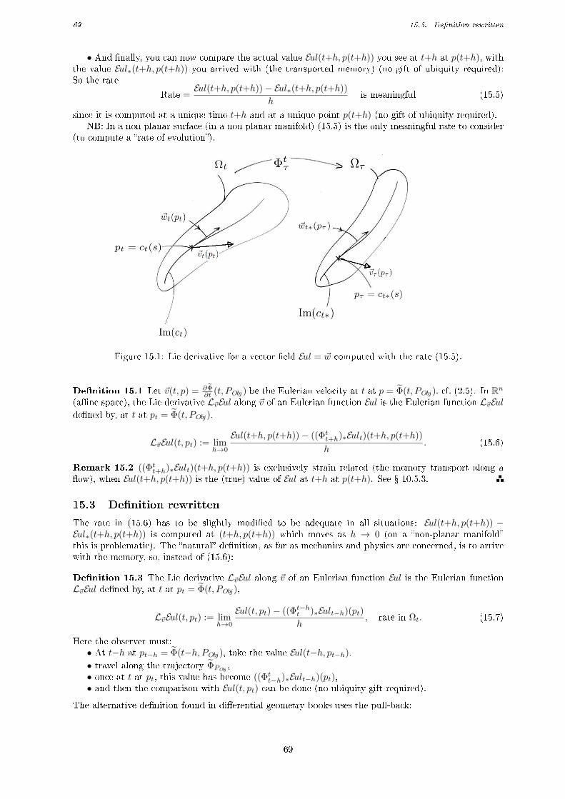
69 15.3. Denition rewritten
• And nally, you can now compare the actual value Eul(t+h, p(t+h)) you see at t+h at p(t+h), withthe value Eul∗(t+h, p(t+h)) you arrived with (the transported memory) (no gift of ubiquity required):So the rate
Rate =Eul(t+h, p(t+h))− Eul∗(t+h, p(t+h))
his meaningful (15.5)
since it is computed at a unique time t+h and at a unique point p(t+h) (no gift of ubiquity required).NB: In a non planar surface (in a non planar manifold) (15.5) is the only meaningful rate to consider
(to compute a rate of evolution).
Figure 15.1: Lie derivative for a vector eld Eul = ~w computed with the rate (15.5).
Denition 15.1 Let ~v(t, p) = ∂Φ∂t (t, PObj ) be the Eulerian velocity at t at p = Φ(t, PObj ), cf. (2.5). In Rn
(ane space), the Lie derivative L~vEul along ~v of an Eulerian function Eul is the Eulerian function L~vEuldened by, at t at pt = Φ(t, PObj ),
L~vEul(t, pt) := limh→0
Eul(t+h, p(t+h))− ((Φtt+h)∗Eult)(t+h, p(t+h))
h. (15.6)
Remark 15.2 ((Φtt+h)∗Eult)(t+h, p(t+h)) is exclusively strain related (the memory transport along aow), when Eul(t+h, p(t+h)) is the (true) value of Eul at t+h at p(t+h). See 10.5.3.
15.3 Denition rewritten
The rate in (15.6) has to be slightly modied to be adequate in all situations: Eul(t+h, p(t+h)) −Eul∗(t+h, p(t+h)) is computed at (t+h, p(t+h)) which moves as h → 0 (on a non-planar manifoldthis is problematic). The natural denition, as far as mechanics and physics are concerned, is to arrivewith the memory, so, instead of (15.6):
Denition 15.3 The Lie derivative L~vEul along ~v of an Eulerian function Eul is the Eulerian functionL~vEul dened by, at t at pt = Φ(t, PObj ),
L~vEul(t, pt) := limh→0
Eul(t, pt)− ((Φt−ht )∗Eult−h)(pt)
h, rate in Ωt. (15.7)
Here the observer must:• At t−h at pt−h = Φ(t−h, PObj ), take the value Eul(t−h, pt−h),
• travel along the trajectory ΦPObj,
• once at t at pt, this value has become ((Φtt−h)∗Eult−h)(pt),• and then the comparison with Eul(t, pt) can be done (no ubiquity gift required).
The alternative denition found in dierential geometry books uses the pull-back:
69
70 15.4. Lie derivative of a scalar function
Denition 15.4 The Lie derivative of a Eulerian function Eul along a ow of Eulerian velocity ~v is theEulerian function L~vEul dened at (t, pt) by
L~vEul(t, pt) := limh→0
((Φtt+h)∗Eult+h)(pt)− Eult(pt)h
, rate in Ωt. (15.8)
In other words, if g is a a function dened by
g(τ) = ((Φtτ )∗Eulτ )(pt) (15.9)
(in particular g(t) = Eul(t, pt)), then (15.8) reads
L~vEul(t, pt) := g′(t) = limτ→t
g(τ)− g(t)
τ − talso written
=d((Φtτ )∗Eulτ )(pt)
dτ |τ=t. (15.10)
NB: (15.7) and (15.8) are equivalent since (15.8) also reads (with h→ −h)
L~vEul(t, pt) = limh→0
((Φtt−h)∗Eult−h)(pt)− Eult(pt)−h
= limh→0
Eult(pt)− ((Φtt−h)∗Eult−h)(pt)
h, (15.11)
and (Φtt−h)∗ = ((Φtt−h)−1)∗ = (Φt−ht )∗, cf. e.g. (10.37) and (3.7).
Remark 15.5 More precise denition, as in (2.3): E.g. with (15.8), the Lie derivative L~vEul of a Eulerianfunction Eul along a ow of Eulerian velocity ~v is dened by, at t at pt = Φ(t, PObj ),
L~vEul(t, pt) := ((t, pt),L~vEul(t, pt)︸ ︷︷ ︸function at t at pt
. (15.12)
(And, to lighten the notation, L~vEul(t, pt) =named L~vEul(t, pt).)
Remark 15.6 In the ane manifold Rn, the tangent spaces are all identied with the vector space ~Rn,and the denition of L~vEul given by (15.6) is equivalent to the denition given by (15.8): E.g. for vector
elds ~w, with p(t+h) = Φtt+h(pt) we have~wt+h(p(t+h))−((Φtt+h)∗ ~wt)(p(t+h))
h =~wt+h(p(t+h))−dΦtt+h(pt). ~wt(pt)
h =
dΦtt+h(pt).dΦtt+h(pt)
−1. ~wt+h(p(t+h))−~wt(pt)h = dΦtt+h(pt).
((Φtt+h)∗ ~wt+h)(pt)−~wt(pt)h , and dΦtt+h(pt)−→h→0 I.
15.4 Lie derivative of a scalar function
Let f be a C1 Eulerian scalar function, let p(τ) = Φ(τ, PObj ) = pτ . Then (10.10) gives (Φt−ht )∗ft−h)(pt) =ft−h(pt−h), thus (15.8) gives
L~vf(t, pt) = limh→0
f(t, p(t))− f(t−h, p(t−h))
h= limh→0
f(t+h, p(t+h))− f(t, p(t))
h=Df
Dt(t, pt), (15.13)
hence, cf. (2.27),
L~vf =Df
Dt=∂f
∂t+ df.~v. (15.14)
Thus for scalar functions, the Lie derivative is the material derivative.
Interpretation: f(t, p(t)) is the value of f at the actual time t at p(t), whereas f(t−h, p(t−h)) is thetransported memory (the value f had at t−h at pt−h). Thus L~vf measures the evolution of f along atrajectory.
Proposition 15.7Df
Dt= 0 in C ⇐⇒ ∀t, τ ∈ [t0, T ], fτ = (Φtτ )∗ft. (15.15)
That is, DfDt = 0 i f let itself be carried by the ow, i.e., if f(t, p(t)) = f(t0, p(t0)) for all t.
Proof. Let p(t) = Φ(t, PObj ) = pt and p(τ) = Φ(τ, PObj ) = pτ , thus pτ = Φtt+h(pt) = Φt(τ, pt).
⇐: If fτ = (Φtt+h)∗ft, then fτ (pτ ) = ft(pt), thus limτ→tf(τ,p(τ))−f(t,p(t))
τ−t = 0, that is, DfDt = 0.
⇒: If DfDt = 0 then f(t, p(t)) is a constant function on the trajectory t → Φ(t, PObj ), for any parti-
cle PObj , so f(τ, p(τ)) = f(t, pt) when p(τ) = Φtt+h(pt), that is, f(τ, pτ ) = (Φtt+h)∗ft(pτ ).
70
71 15.5. Lie derivative of a vector eld
Exercice 15.8 Prove:
L~v(L~vf) =D2f
Dt2=∂2f
∂t2+ 2d(
∂f
∂t).~v + d2f(~v,~v) + df.(
∂~v
∂t+ d~v). (15.16)
Answer. See (2.48).
15.5 Lie derivative of a vector eld
Let ~w be a C1 (Eulerian) vector eld, e.g. interpreted as a force eld.
Proposition 15.9
L~v ~w =D~w
Dt− d~v.~w =
∂ ~w
∂t+ d~w.~v − d~v.~w. (15.17)
Thus the Lie derivative is not reduced to the material derivative D~wDt (unless d~v = 0, i.e. unless ~v is
uniform): The spatial variations of ~v inuences the rate of stress, which is expected.
Proof. E.g., with (15.8): Let ~g : τ → ~g(τ) = (Φt∗τ ~w)(t, p(t)) = dΦtτ (pt)−1. ~w(τ, p(τ)) when p(τ) =
Φt(τ, pt). Then (15.8) reads:L~v ~w(t, pt) = ~g ′(t). (15.18)
Since ~z(τ) := ~w(τ, p(τ)) = dΦt(τ, pt).~g(τ) we get
~z ′(τ) =D~w
Dτ(τ, p(τ)) =
∂(dΦt)
∂τ(τ, pt).~g(τ) + dΦt(τ, pt).~g
′(τ)
= (d~v(τ, p(τ)).F t(τ, pt)).(Ft(τ, pt)
−1. ~w(τ, p(τ))) + F tτ (pt).~g′(τ)
= d~v(τ, p(τ)). ~w(τ, p(τ)) + F tτ (pt).~g′(τ).
(15.19)
Thus D~wDt (t, pt) = d~v(t, pt). ~w(t, pt) + I.~g ′(t) = d~v(t, pt). ~w(t, pt) + L~v ~w(t, pt), i.e. (15.17).
Remark 15.10 A function f : p→ f(p) ∈ R gives scalar values f(p), and a scalar f(p) has no direction.Thus f(p) is not sensitive to the variations d~v of ~v: There is no d~v term in (15.14).
While a vector valued function ~w : p → ~w(p) ∈ ~Rn gives vector values ~w(p), and a vector ~w(p) hasa direction. And, submitted to a ow, ~w(p) is sensitive to the variations of the ow: The −d~v.~w termattests it. (A vector is not just a collection of scalar components.)
Remark 15.11 The Cauchy expression ~t = σ.~n states that the Cauchy stress vector is a linear functionof the normal vector ~n to a surface, meaning that a surface is considered to be locally planar (rst orderTaylor expansion), thus excludes second order eects (curvature eect). While the Lie approach does notmake such hypothesis (and we can use L~v(L~v ~w) for second order terms).
Remark 15.12 The Lie bracket of two vector elds ~v and ~w is
[~v, ~w] := d~w.~v − d~v.~w noted= L0
~v ~w. (15.20)
And L0~v ~w is called the autonomous Lie derivative of ~w along ~v. Thus
L~v ~w =∂ ~w
∂t+ [~v, ~w] =
∂ ~w
∂t+ L0
~v ~w. (15.21)
NB: L0~v ~w is used when ~v et ~w are stationary vector elds, thus does not concern objectivity: A stationary
vector eld in a referential is not necessary stationary in another (moving) referential.
71
72 15.6. Examples and interpretations
15.6 Examples and interpretations
15.6.1 Flow resistance measurement
Proposition 15.13
L~v ~w = 0 ⇐⇒ D~w
Dt= d~v.~w ⇐⇒ ∀t, τ ∈ [t0, T ], ~wτ = (Φtτ )∗ ~wt. (15.22)
Interpretation with (15.7):• ~w(t, p(t)) is the actual value of the force eld ~w at t at p(t),• whereas the push-forward ~wt−h∗(t, p(t)) is the transported memory = the virtual value that ~w
would have had at t at p(t) if it had let itself be carried by the ow (strain dependent, see (10.26)-(10.28)).• So (15.22) means: The Lie derivative L~v ~w vanishes i ~w does not resist the ow (let itself be
deformed by the ow).
Proof. ⇐: If ~wτ (p(τ)) = F tτ (pt). ~wt(pt) then ~w(τ, p(τ)) = F t(τ, pt). ~w(t, pt), thus D~wDτ (τ, p(τ)) =
∂(F t)∂τ (τ, pt). ~w(t, pt) = (d~v(τ, p(τ)).F tτ (pt)).(F
tτ (pt)
−1. ~w(τ, p(τ))) = d~v(τ, p(τ)). ~w(τ, p(τ)), thus D~wDt −
d~v.~w = 0. (See proposition 4.10.)
⇒: Let ~f(τ, t, p(t)) = F tτ (p(t))−1. ~wτ (p(τ)) be the pull-back of ~wτ by Φtτ at p(t) =
(Φtτ )−1(p(τ)). Then ~w(τ, p(τ)) = F t(τ, pt). ~f(τ, t, pt) when p(τ) = Φt(τ, pt). Thus D~wDτ (τ, p(τ)) =
(d~v(τ, p(τ)).F t(τ, p(t))). ~f(τ, t, p(t)) +F t(τ, p(t)).∂~f
∂τ (τ, t, p(t)), thus D~wDτ (τ, p(τ)) = d~v(τ, p(τ)). ~w(τ, p(t)) +
F t(τ, p(t)).∂~f
∂τ (τ, t, p(t)). Thus L~v ~w = 0 gives F t(τ, p(t)).∂~f
∂τ (τ) = 0, thus ∂ ~f∂τ (τ, t, p(t)) = 0 since Φtt+h is a
dieomorphism. Thus ∂ ~f∂τ (τ, t, p(t)) is independent of τ , thus ~f(τ, t, p(t)) = ~f(t, t, p(t)) = ~wt(p(t)). Thus
~wt is the pull-back of ~wτ .
15.6.2 Lie Derivative of a vector eld along itself
(15.17) gives
L~v~v =∂~v
∂t. (15.23)
In particular, if ~v is a stationary vector eld, then
L~v~v = ~0. (15.24)
This is also a direct consequence of (6.24).
15.6.3 Lie derivative along a uniform ow
Suppose d~v = 0. Then note ~v(t, p) = ~v(t) (e.g., ~v(t, p) = λ(t)~e1 where (~ei) is a Cartesian basis). Then
L~v ~w =∂ ~w
∂t+ d~w.~v =
D~w
Dt(here d~v = 0). (15.25)
In this case the ow is rectilinear (d~v = 0): there is no curvature (of the ow) to inuence the stresson ~w.
Moreover, if ~w is stationary, that is ∂ ~w∂t = 0, then
L~v ~w = d~w.~v (15.26)
= the directional derivative of the vector eld ~w in the direction ~v.
15.6.4 Lie derivative of a uniform vector eld
Suppose d~w(t, p) = 0. Then
L~v ~w =∂ ~w
∂t− d~v.~w (here d~w = 0), (15.27)
thus the stress on ~w is due to the space variations of ~v (due to the curvature of the ow). Moreover, is~w is stationary then
L~v ~w = −d~v.~w. (15.28)
(See remark 15.11.)
72
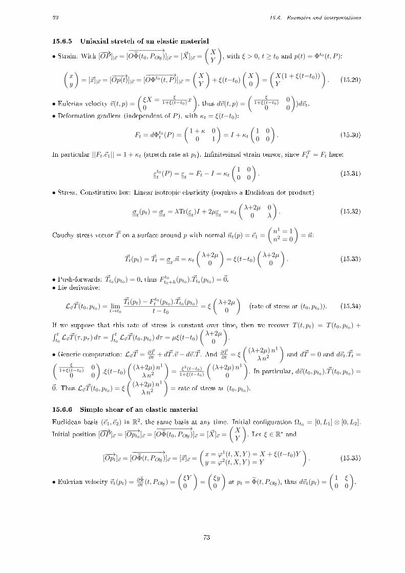
73 15.6. Examples and interpretations
15.6.5 Uniaxial stretch of an elastic material
• Strain. With [−−→OP ]|~e = [
−−−−−−−−→OΦ(t0, PObj )]|~e = [ ~X]|~e =
(XY
), with ξ > 0, t ≥ t0 and p(t) = Φt0(t, P ):
(xy
)= [~x]|~e = [
−−−→Op(t)]|~e = [
−−−−−−−→OΦt0(t, P )]|~e =
(XY
)+ ξ(t−t0)
(X0
)=
(X(1 + ξ(t−t0))Y
). (15.29)
• Eulerian velocity ~v(t, p) =
(ξX = ξ
1+ξ(t−t0)x0
), thus d~v(t, p) =
(ξ
1+ξ(t−t0) 00 0
))d~vt.
• Deformation gradient (independent of P ), with κt = ξ(t−t0):
Ft = dΦt0t (P ) =
(1 + κ 0
0 1
)= I + κt
(1 00 0
). (15.30)
In particular ||Ft.~e1|| = 1 + κt (stretch rate at pt). Innitesimal strain tensor, since FTt = Ft here:
εt0t
(P ) = εt
= Ft − I = κt
(1 00 0
). (15.31)
• Stress. Constitutive law: Linear isotropic elasticity (requires a Euclidean dot product)
σt(pt) = σ
t= λTr(ε
t)I + 2µε
t= κt
(λ+2µ 0
0 λ
). (15.32)
Cauchy stress vector ~T on a surface around p with normal ~nt(p) = ~e1 =
(n1 = 1n2 = 0
)= ~n:
~Tt(pt) = ~Tt = σt.~n = κt
(λ+2µ
0
)= ξ(t−t0)
(λ+2µ
0
). (15.33)
• Push-forwards: ~Tt0(pt0) = 0, thus F t0t0+h(pt0). ~Tt0(pt0) = ~0.• Lie derivative:
L~v ~T (t0, pt0) = limt→t0
~Tt(pt)− F t0t (pt0). ~Tt0(pt0)
t− t0= ξ
(λ+2µ
0
)(rate of stress at (t0, pt0)). (15.34)
If we suppose that this rate of stress is constant over time, then we recover T (t, pt) = T (t0, pt0) +∫ tt0L~v ~T (τ, pτ ) dτ =
∫ tt0L~v ~T (t0, pt0) dτ = µξ(t−t0)
(λ+2µ
0
).
• Generic computation: L~v ~T = ∂ ~T∂t + d~T .~v − d~v.~T . And ∂ ~T
∂t = ξ
((λ+2µ)n1
λn2
)and d~T = 0 and d~vt. ~Tt =(
ξ1+ξ(t−t0) 0
0 0
).ξ(t−t0)
((λ+2µ)n1
λn2
)= ξ2(t−t0)
1+ξ(t−t0)
((λ+2µ)n1
0
). In particular, d~v(t0, pt0). ~T (t0, pt0) =
~0. Thus L~v ~T (t0, pt0) = ξ
((λ+2µ)n1
λn2
)= rate of stress at (t0, pt0).
15.6.6 Simple shear of an elastic material
Euclidean basis (~e1, ~e2) in R2, the same basis at any time. Initial conguration Ωt0 = [0, L1] ⊗ [0, L2].
Initial position [−−→OP ]~e = [
−−→Opt0 ]~e = [
−−−−−−−−→OΦ(t0, PObj )]~e = [ ~X]~e =
(XY
). Let ξ ∈ R∗ and
[−−→Opt]~e = [
−−−−−−−−→OΦ(t, PObj )]~e = [~x]~e =
(x = ϕ1(t,X, Y ) = X + ξ(t−t0)Yy = ϕ2(t,X, Y ) = Y
). (15.35)
• Eulerian velocity ~vt(pt) = ∂Φ∂t (t, PObj ) =
(ξY0
)=
(ξy0
)at pt = Φ(t, PObj ), thus d~vt(pt) =
(1 ξ0 0
).
73
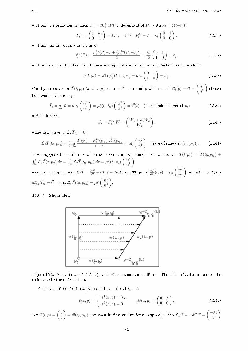
74 15.6. Examples and interpretations
• Strain. Deformation gradient Ft = dΦt0t (P ) (independent of P ), with κt = ξ(t−t0):
F t0t =
(1 κt0 1
)= F t0t , thus F t0t − I = κt
(0 10 0
). (15.36)
• Strain. Innitesimal strain tensor:
εt0t
(P ) =F t0t (P )−I + (F t0t (P )−I)T
2=κt2
(0 11 0
)= ε
t. (15.37)
• Stress. Constitutive law, usual linear isotropic elasticity (requires a Euclidean dot product):
σ(t, pt) = λTr(εt)I + 2µε
t= µκt
(0 11 0
)= σ
t. (15.38)
Cauchy stress vector ~T (t, pt) (at t at pt) on a surface around p with normal ~nt(p) = ~n =
(n1
n2
)chosen
independent of t and p:
~Tt = σt.~n = µκt
(n2
n1
)= µξ(t−t0)
(n2
n1
)= ~T (t) (stress independent of pt). (15.39)
• Push-forward~w∗ = F t0t . ~W =
(W1 + κtW2
W2
), (15.40)
• Lie derivative, with ~Tt0 = ~0:
L~v ~T (t0, pt0) = limt→t0
~Tt(pt)− F t0t (pt0). ~Tt0(pt0)
t− t0= µξ
(n2
n1
)(rate of stress at (t0, pt0)). (15.41)
If we suppose that this rate of stress is constant over time, then we recover ~T (t, pt) = ~T (t0, pt0) +∫ tt0L~v ~T (τ, pτ ) dτ =
∫ tt0L~v ~T (t0, pt0) dτ = µξ(t−t0)
(n2
n1
).
• Generic computation: L~v ~T = ∂ ~T∂t + d~T .~v − d~v.~T . (15.39) gives ∂ ~T
∂t (t, p) = µξ
(n2
n1
)and d~T = 0. With
d~vt0 .~Tt0 = ~0. Thus L~v ~T (tz, pt0) = µξ
(n2
n1
).
15.6.7 Shear ow
Figure 15.2: Shear ow, cf. (15.42), with ~w constant and uniform. The Lie derivative measures theresistance to the deformation.
Stationary shear eld, see (6.11) with α = 0 and t0 = 0:
~v(x, y) =
v1(x, y) = λy,
v2(x, y) = 0,d~v(x, y) =
(0 λ0 0
). (15.42)
Let ~w(t, p) =
(0b
)= ~w(t0, pt0) (constant in time and uniform in space). Then L~v ~w = −d~v.~w =
(−λb
0
)
74
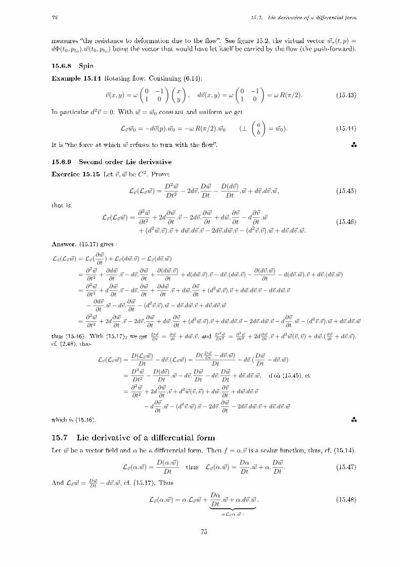
75 15.7. Lie derivative of a dierential form
measures the resistance to deformation due to the ow. See gure 15.2, the virtual vector ~w∗(t, p) =dΦ(t0, pt0). ~w(t0, pt0) being the vector that would have let itself be carried by the ow (the push-forward).
15.6.8 Spin
Example 15.14 Rotating ow: Continuing (6.14):
~v(x, y) = ω
(0 −11 0
)(xy
), d~v(x, y) = ω
(0 −11 0
)= ωR(π/2). (15.43)
In particular d2~v = 0. With ~w = ~w0 constant and uniform we get
L~v ~w0 = −d~v(p). ~w0 = −ωR(π/2). ~w0 (⊥(ab
)= ~w0). (15.44)
It is the force at which ~w refuses to turn with the ow.
15.6.9 Second order Lie derivative
Exercice 15.15 Let ~v, ~w be C2. Prove:
L~v(L~v ~w) =D2 ~w
Dt2− 2d~v.
D~w
Dt− D(d~v)
Dt.~w + d~v.d~v.~w, (15.45)
that is,
L~v(L~v ~w) =∂2 ~w
∂t2+ 2d
∂ ~w
∂t.~v − 2d~v.
∂ ~w
∂t+ d~w.
∂~v
∂t− d∂~v
∂t.~w
+ (d2 ~w.~v).~v + d~w.d~v.~v − 2d~v.d~w.~v − (d2~v.~v). ~w + d~v.d~v.~w.
(15.46)
Answer. (15.17) gives :
L~v(L~v ~w) = L~v(∂ ~w
∂t) + L~v(d~w.~v)− L~v(d~v.~w)
=∂2 ~w
∂t2+∂d~w
∂t.~v − d~v.∂ ~w
∂t+∂(d~w.~v)
∂t+ d(d~w.~v).~v − d~v.(d~w.~v)− ∂(d~v.~w)
∂t− d(d~v.~w).~v + d~v.(d~v.~w)
=∂2 ~w
∂t2+ d
∂ ~w
∂t.~v − d~v.∂ ~w
∂t+∂d~w
∂t.~v + d~w.
∂~v
∂t+ (d2 ~w.~v).~v + d~w.d~v.~v − d~v.d~w.~v
− ∂d~v
∂t. ~w − d~v.∂ ~w
∂t− (d2~v.~v). ~w − d~v.d~w.~v + d~v.d~v.~w
=∂2 ~w
∂t2+ 2d
∂ ~w
∂t.~v − 2d~v.
∂ ~w
∂t+ d~w.
∂~v
∂t+ (d2 ~w.~v).~v + d~w.d~v.~v − 2d~v.d~w.~v − d∂~v
∂t. ~w − (d2~v.~v). ~w + d~v.d~v.~w
thus (15.46). With (15.17)2 we get D~wDt
= ∂ ~wdt
+ d~w.~v, and D2 ~wDt2
= ∂2 ~w∂t2
+ 2d ∂ ~w∂t.~v + d2 ~w(~v,~v) + d~w.( ∂~v
dt+ d~v.~v),
cf. (2.48), thus
L~v(L~v ~w) =D(L~v ~w)
Dt− d~v.(L~v ~w) =
D(D~wDt− d~v.~w)
Dt− d~v.(D~w
Dt− d~v.~w)
=D2 ~w
Dt2− D(d~v)
Dt.~w − d~v.D~w
Dt− d~v.D~w
Dt+ d~v.d~v.~w, d'où (15.45), et
=∂2 ~w
∂t2+ 2d
∂ ~w
∂t.~v + d2 ~w(~v,~v) + d~w.
∂~v
∂t+ d~w.d~v.~v
− d∂~v∂t. ~w − (d2~v.~w).~v − 2d~v.
∂ ~w
∂t− 2d~v.d~w.~v + d~v.d~v.~w
which is (15.46).
15.7 Lie derivative of a dierential form
Let ~w be a vector eld and α be a dierential form. Then f = α.~v is a scalar function, thus, cf. (15.14),
L~v(α.~w) =D(α.~w)
Dtthus L~v(α.~w) =
Dα
Dt.~w + α.
D~w
Dt. (15.47)
And L~v ~w = D~wDt − d~v.~w, cf. (15.17). Thus
L~v(α.~w) = α.L~v ~w +Dα
Dt.~w + α.d~v.~w︸ ︷︷ ︸=L~vα.~w :
. (15.48)
75
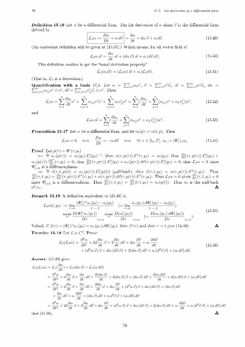
76 15.7. Lie derivative of a dierential form
Denition 15.16 Let α be a dierential form. The Lie derivative of α along ~v is the dierential formdened by
L~vα :=Dα
Dt+ α.d~v =
∂α
∂t+ dα.~v + α.d~v. (15.49)
(An equivalent denition will be given at (15.55).) Which means, for all vector eld ~w,
L~vα.~w =∂α
∂t.~w + (dα.~v). ~w + α.(d~v.~w). (15.50)
This denition enables to get the usual derivation property
L~v(α.~w) = (L~vα). ~w + α.(L~v ~w). (15.51)
(That is, L~v is a derivation.)
Quantication with a basis (~ei): Let α =∑ni=1αie
i, ~v =∑ni=1v
i~ei, ~w =∑ni=1w
i~ei, dα =∑ni,j=1αi|je
i ⊗ ej , d~v =∑ni,j=1v
i|j~ei ⊗ e
j . Then
L~vα =
n∑i=1
∂αi∂t
ei +
n∑i,j=1
αi|jvjei +
n∑i,j=1
αivi|je
j =
n∑i=1
(∂αi∂t
+
n∑j=1
(αi|jvj + αjv
j|i))e
i, (15.52)
and
L~vα.~w =
n∑i=1
(∂αi∂t
+
n∑j=1
(αi|jvj + αjv
j|i))w
i. (15.53)
Proposition 15.17 Let α be a dierential form, and let αt(p) := α(t, p). Then
L~vα = 0 ⇐⇒ Dα
Dt= −α.d~v ⇐⇒ ∀t, τ ∈ [t0, T ], ατ = (Φtτ )∗αt. (15.54)
Proof. Let p(τ) = Φt(τ, pt)⇐: If ατ (p(τ)) = αt(pt).F
tτ (pt)
−1, then α(τ, p(τ)).F t(τ, pt) = αt(pt), thus DαDτ (τ, p(τ)).F tτ (pt) +
ατ (p(τ)).∂Ft
∂τ (τ, pt) = 0, thus DαDτ (τ, p(τ)).F tτ (pt) + ατ (p(τ)).d~v(τ, p(τ)).F tτ (pt) = 0, thus L~vα = 0 since
Φtt+h is a dieomorphism.⇒: If β(τ, t, p(t)) = ατ (p(τ)).F tτ (p(t)) (pull-back), then β(τ, t, pt) = α(τ, p(τ)).F t(τ, pt). Thus
∂β∂τ (τ, t, pt) = Dα
Dτ (τ, p(τ)).F t(τ, pt) + α(τ, p(τ)).d~v(τ, p(τ)).F t(τ, pt). Thus L~vα = 0 gives ∂β∂τ (τ, t, pt) = 0
since Φtt+h is a dieomorphism. Thus ∂β∂τ (τ, t, pt) = ∂β
∂τ (t, t, pt) = αt(p(t)). Thus αt is the pull-backof ατ .
Remark 15.18 A denition equivalent to (15.49) is
L~vα(t, pt) := limτ→t
(Φtτ )∗ατ (pt)− αt(pt)τ − t
(= limτ→t
ατ (pτ ).dΦtτ (pt)− αt(pt)τ − t
)
noted=
D(Φt∗τ ατ (pt))
Dτ |τ=t
noted=
D(α∗τ (pt))
Dτ |τ=t(=
D(ατ (pτ ).dΦtτ (pt))
Dτ |τ=t).
(15.55)
Indeed, if β(τ) = (Φtτ )∗ατ (pt) = ατ (pτ ).dΦtτ (pt), then β′(τ) and then τ = t give (15.49).
Exercice 15.19 Let ~v, α C2. Prove:
L~v(L~vα) =∂2α
∂t2+ 2d
∂α
∂t.~v + 2
∂α
∂t.d~v + dα.
∂~v
∂t+ α.
∂d~v
∂t
+ (d2α.~v).~v + dα.(d~v.~v) + 2(dα.~v).d~v + α.(d2~v.~v) + (α.d~v).d~v.
(15.56)
Answer. (15.49) gives
L~v(L~vα) = L~v(∂α
∂t) + L~v(dα.~v) + L~v(α.d~v)
=∂2α
∂t2+ d
∂α
∂t.~v +
∂α
∂t.d~v +
∂(dα.~v)
∂t+ d(dα.~v).~v + (dα.~v).d~v +
∂(α.d~v)
∂t+ d(α.d~v).~v + (α.d~v).d~v
=∂2α
∂t2+ d
∂α
∂t.~v +
∂α
∂t.d~v +
∂dα
∂t.~v + dα.
∂~v
∂t+ (d2α.~v).~v + dα.(d~v.~v) + (dα.~v).d~v
+∂α
∂t.d~v + α.
∂d~v
∂t+ (dα.~v).d~v + α.d2~v.~v + (α.d~v).d~v
=∂2α
∂t2+ 2d
∂α
∂t.~v + 2
∂α
∂t.d~v + dα.
∂~v
∂t+ (d2α.~v).~v + dα.(d~v.~v) + 2(dα.~v).d~v + α.
∂d~v
∂t+ α.(d2~v.~v) + (α.d~v).d~v
thus (15.56).
76
77 15.8. Incompatibility with the representation vector
15.8 Incompatibility with the representation vector
The Lie derivative has nothing to do with any inner dot product (the Lie derivative does not compare twovectors to get a stress, contrary to a Cauchy type approach). But here, to deal with the classic literature,we consider a Euclidean dot product g(·, ·) =named(·, ·)g.
Let α a dierential form. Let ~αg(t, p) ∈ ~Rn be the (·, ·)g-Riesz representation vector of the linearform α(t, p), that is,
∀~w ∈ ~Rnt , α(t, p). ~w = (~αg(t, p), ~w)g. (15.57)
This denes the (Eulerian) vector eld ~αg (observer dependent since it depends on the choice of aEuclidean dot product, cf. (B.8): ~αg is not intrinsic to α).
Proposition 15.20 For all ~v, ~w ∈ ~Rn,∂α
∂t.~w = (
∂~αg∂t
, ~w)g, (dα.~v). ~w = (d~αg.~v, ~w)g,Dα
Dt.~w = (
D~αgDt
, ~w)g. (15.58)
ThusL~vα.~w = (L~v~αg, ~w)g + (~αg, (d~v + d~vT ). ~w)g
6= (L~v~αg, ~w)g in general.(15.59)
So L~v~αg isn't the Riesz representation vector of L~vα. (This is expected: A Lie derivative is covariantobjective, see 18.7, which is incompatible with the use of an inner dot product which ruins objectivity.)
Proof. g(·, ·) being constant and uniform (it is a Euclidean dot product: It is a metric independent of tand p), (15.57) immediately gives (15.58)1,2, thus (15.58)3.
Remark 15.21 So, to confuse dierential forms (covariance) and vector elds (contravariance), be-cause of the use of an inner dot product (which one?) and Riesz's representation theorem, creates errorswhen using the Lie derivative. See also C.3. It has consequences for constitutive laws of uids (usuallymodeled with vector elds) and for constitutive laws of solids (usually modeled with dierential forms).
Exercice 15.22 In (15.59) when do we have L~vα.~w = (L~v~αg, ~w)g?
Answer. When, for all ~w ∈ Rn,∂α
∂t. ~w + (dα.~v). ~w + α.d~v.~w = (
∂~αg∂t
, ~w)g + (d~αg.~v, ~w)g − (d~v.~αg, ~w)g. (15.60)
So when α.d~v.~w = −(d~v.~αg, ~w)g, i.e.α.d~v.~w = −(~αg, d~vTg . ~w)g = −α.(d~vTg . ~w) for all ~w, i.e. α.(d~v+d~vTg ) = 0, e.g.
for a solid body motion.
Exercice 15.23 Prove (15.58)2 with a (·, ·)g-orthonormal basis (~ei).
Answer. Let (ei) be the dual basis. Let α =∑i αie
i, ~αg =∑i zi~ei, ~v =
∑i vi~ei, ~w =
∑i w
i~ei. Thus
dα =∑ij∂αi∂xj
ei⊗ ej , d~αg =∑ij∂zi
∂xj~ei⊗ ej , d~v =
∑ij∂vi
∂xj~ei⊗ ej . Thus dα.~v =
∑ij∂αi∂xj
vjei, α.d~v =∑ij αi
∂vi
∂xjej ,
d~αg.~v =∑ij∂zi
∂xjvjei, d~v.~αg =
∑ij∂vi
∂xjzjei. And (15.57) gives zi = αi for all i (orthonormal basis).
Thus ( ∂α∂t, ~w)g =
∑i∂αi∂twi =
∑i∂zi
∂twi = (
∂~αg∂t, ~w)g, and (dα.~v). ~w = (
∑ij∂αi∂xj
vjei). ~w =∑ij∂αi∂xj
wivj =∑ij∂zi
∂xjwivj = (
∑ij∂zi
∂xjvjei, ~w)g = (d~αg.~v, ~w)g, i.e. (15.58)2.
15.9 Lie derivative of a tensor
15.9.1 Formula
A tensor is dened with vector elds and dierential forms. That makes it possible to dene the Liederivative of any tensor with one of the equivalent denitions:
L~v(T ⊗ S) = (L~vT )⊗ S + T ⊗ (L~vS), or L~vT (t0, pt0) =D((Φt0t )∗Tt)(pt0)
Dt |t=t0. (15.61)
15.9.2 Lie derivative of a mixed tensor
Mixed tensor Tm ∈ T 11 (Ω): We get the Lie derivative called the Jaumann derivative:
L~vTm =DTmDt
− d~v.Tm + Tm.d~v =∂Tm∂t
+ dTm.~v − d~v.Tm + Tm.d~v. (15.62)
Can be checked with an elementary tensor T = ~w ⊗ α and L~v(~w ⊗ α) = (L~v ~w)⊗ α+ ~w ⊗ (L~vα).
77
78 15.9. Lie derivative of a tensor
15.9.3 For a non mixed tensor
For non mixed tensor, we recall:
Denition 15.24 If bil ∈ L(E,F ;R) (bilinear), then its transposed bilT ∈ L(F,E;R) is dened by
∀(~u, ~w) ∈ E × F, bilT (~w, ~u) = bil(~u, ~w) . (15.63)
Denition 15.25 Let L ∈ L(E;F ) (a linear map). Its adjoint L∗ ∈ L(F ∗;E∗) is dened by, cf. A.13,
∀m ∈ F ∗, L∗.m = m.L , i.e. ∀m,~u ∈ (F ∗ × E), (L∗.m).~u = m.(L.~u). (15.64)
(There is no inner dot product involved.) (E.g., with L = d~vt ∈ L(~Rnt ; ~Rnt ), then (d~vt)∗ ∈ L(~Rn∗t ; ~Rn∗t ).)
15.9.4 Lie derivative of a up-tensor
Up tensor: Tu ∈ T 20 (Ω): The Lie derivative is called the Oldroyd or the upper-convected Maxwell
derivative:
L~vTu =DTuDt− d~v.Tu − Tu.d~v∗ =
∂Tu∂t
+ dTu.~v − d~v.Tu − Tu.d~v∗. (15.65)
Can be checked with an elementary tensor T = ~u⊗ ~w and L~v(~u⊗ ~w) = (L~v~u)⊗ ~w + ~u⊗ (L~v ~w).
The up refers to positions of indices when a basis (~ei) in ~Rnt is used: [Tu]|~e = [T ij ], that is,
Tu =∑ni,j=1T
ij~ei⊗~ej . And here d~vt(p) ∈ L(~Rnt ; ~Rnt ) ' L(~Rn∗t , ~Rnt ;R): We have d~vt(p) =∑ni,j=1v
i|j~ei⊗e
j .
And d~v∗t (p) =∑ni,j=1v
j|iei ⊗~ej ∈ L(~Rnt , ~Rn∗t ;R) ' L(~Rn∗t ; ~Rn∗t ). Thus d~v.Tu =
∑ni,j,k=1v
i|kT
kj~ei ⊗~ej , andTu.d~v
∗ =∑ni,j,k=1T
ikvj|k~ei ⊗ ~ej . Thus
[L~vTu]|~e = [DTuDt
]|~e − [d~v]|~e.[Tu]|~e − [Tu]|~e.[d~v]T|~e. (15.66)
15.9.5 Lie derivative of a down-tensor
Down tensor: Td ∈ T 02 (Ω): The Lie derivative is called the lower-convected Maxwell derivative:
L~vTd =DTdDt
+ Td.d~v + d~v∗.Td =∂Td∂t
+ dTd.~v + Td.d~v + d~v∗.Td. (15.67)
Can be checked with an elementary tensor T = `⊗m and L~v(`⊗m) = (L~v`)⊗m+ `⊗ (L~vm).
The down refers to positions of indices when a basis (~ei) in ~Rnt is used: [Td]|~e = [Tij ], that is,
Td =∑ni,j=1Tije
i ⊗ ej . Thus Td.d~v =∑ni,j,k=1Tikv
k|je
i ⊗ ej and d~v∗.Td =∑ni,j,k=1v
k|iTkje
i ⊗ ej . Thus
[L~vTd]|~e = [DTdDt
]|~e + [Td]|~e.[d~v]|~e + [d~v]T|~e.[Td]|~e. (15.68)
Exercice 15.26 Let g = (·, ·)g be a constant and uniform metric (a unique inner dot product for all t, p,e.g., a Euclidean dot product at all t). And with the Riesz representation theorem dene d~v[ ∈ T 0
2 (Ω)from d~v ∈ T 1
1 (Ω) by:dv[(~u, ~w) = (d~v.~w, ~u)g (= (d~vT .~u, ~w)g). (15.69)
Prove:dv[ = g.d~v. (15.70)
Prove:L~vg = d~v[ + (d~v[)T and L~vg = g.d~v + d~v∗.g. (15.71)
If (~ei) is a (·, ·)g-orthonormal basis, prove:
[L~vg]~e = [d~v]~e + [d~v]T~e . (15.72)
Answer. Let (~ei) be a basis, d~v =∑ni,j=1v
i|j~ei ⊗ ej , d~v[ =
∑ni,j=1Tije
i ⊗ ej , g =∑ni,j=1gije
i ⊗ ej . Thus g.d~v =∑ni,j,k=1gikv
k|je
i ⊗ ej , that is (g.d~v)(~ei, ~ej) =∑nk=1gikv
k|j for all i, j. And (15.69) gives dv[(~ei, ~ej) = g(d~v.~ej , ~ei) =
g(∑nk=1v
k|j~ek, ~ei) =
∑nk=1v
k|jgki =
∑nk=1gikv
k|j , thus dv
[(~ei, ~ej) = (g.d~v)(~ei, ~ej) for all i, j, thus (15.70).
Then d(~v[)T (~ei, ~ej) = d~v[(~ej , ~ei) = (g.d~v)(~ej , ~ei) =∑nk=1[g]jk[d~v]k|i =
∑nk=1[d~v ∗]i|k[g]kj (since g(·, ·) is sym-
metric) = (d~v ∗.g)(~ei, ~ej), thus (15.70).(15.67) and (15.70) give L~vg = 0 + g.d~v + d~v∗.g = d~v[ + (d~v[)T , i.e. (15.71).
In particular, if (~ei) is a (·, ·)g-orthonormal basis, then [g]|~e = I, thus (15.72).
78
79
Part IV
Velocity-addition formula and Objectivity
16 Change of referential
16.1 Introduction and problem
Let Obj be a material object. Let PObj ∈ Obj be a particle, and consider its Eulerian velocities ~vA in areferential RA and ~vB in a referential RB , and let ~vD be the velocity of RB in RA (the drive speed =vitesse d'entrainement). The classical expression of the velocity-addition formula is:
(~vA the absolute velocity) = (~vB the relative velocity) + (~vD the drive speed of RB in RA), (16.1)
But (16.1) is problematic (self contradictory):1- The velocities ~vA and ~vD are velocities in RA: E.g., expressed in foot/s by the absolute observer.2- The velocity ~vB is a velocity in RB : E.g., expressed in meter/s by the relative observer.3- Thus (16.1) seems to indicate that the right hand side adds meter/s with foot/s, which is absurd.Thus ~vB cannot just be the velocity in the relative referential: It has to be the translated velocity
for observer A. Details and explanations:
16.2 Framework
Classical mechanics. The same universe for all observers, modeled as an ane space Rn with the associ-ated vector space ~Rn (made of bipoint vectors), with n = 3, or with n = 1 or 2 if 1-D or 2-D problems arestudied. To lighten the writing, the observers use the same time scale and same time origin (otherwisewe need to dene referentials in R4 = R× Rn = time × space).
An observer A chooses a point OA ∈ Rn (origin), a basis ( ~Ai) ∈ ~Rn to build his referential RA =
(OA, ( ~Ai)), the same at all time. And an observer B chooses a point OB ∈ Rn (origin), a basis ( ~Bi) ∈ ~Rnto build his referential RB = (OB , ( ~Bi)), the same at all time. Illustration: They both live on rigid like
bodies, e.g., with OA the center of the sun and ( ~Ai) xed relative to stars, and OB some point on Earth
and ( ~Bi) xed on Earth.Observers A and B observe the same deformable material object Obj . The position of a particle
PObj ∈ Obj in the ane space Rn is given thanks to motions, cf. (1.2): The motion of Obj is described
by observer A as being ΦA : [t1, t2] × Obj → RA, and is called the absolute motion, and the associatedEulerian velocity eld ~vA is called the absolute velocity eld. And the motion of Obj is described byobserver B as being ΦB : [t1, t2] × Obj → RB , and is called the relative motion, and the associatedEulerian velocity eld ~vB is called the relative velocity eld. So, (1.2) and (2.5) give, for any particlePObj ∈ Obj and any t ∈ [t1, t2],
pAt = ΦA(t, PObj ) = OA +
n∑i=1
xiAt ~Ai = position of PObj at t located by A in RA,
~vA(t, pAt) =∂ΦA∂t
(t, PObj ) = velocity of PObj at t at pAt in RA,
pBt = ΦB(t, PObj ) = OB +
n∑i=1
xiBt ~Bi = position of PObj at t located by B in RB ,
~vB(t, pBt) =∂ΦB∂t
(t, PObj ) = velocity of PObj at t at pBt in RB .
(16.2)
Let ObjB be a material rigid body on which RB is xed (e.g. ObjB = the Earth). The rigid body
motion of ObjB is described by observer A as being ΦD : [t1, t2] × ObjB → RA, and is called the drivemotion (mouvement d'entrainement), and the associated Eulerian velocity eld ~vD is called the drive
velocity eld. The rigid body motion of ObjB is described by observer B as being Ψ : ObjB → RB (staticfunction which locates the particles QObjB ∈ ObjB in the referential chosen by B), and the associated
79
80 16.3. The translator Θt for positions
Eulerian velocity eld vanishes. So, (1.2) and (2.5) give, for any particle QObjB ∈ ObjB and any t ∈ [t1, t2],
qAt = ΦD(t, QObjB) = OA +
n∑i=1
yiAt~Ai = position of QObjB at t located by A in RA,
~vD(t, qAt) =∂ΦD∂t
(t, QObjB) = velocity of QObjB at t at qAt in RA,
qB = ΨB(QObjB) = OB +
n∑i=1
yiB ~Bi = (static) position of QObjB located by B in RB ,
~0 =∂ΨB∂t
(QObjB) = nul velocity since QObjB does not move in RB .
(16.3)
If t is xed, then let ΦZt(PObj ) := ΦZ(t, PObj ) and ~vZt(pZt) := ~vZ(t, pZt) and ΩZt := ΦZ(t, PObj ), forZ = A,B,D.
The drive motion ΦD being a rigid body motion, we have, for all qAit = ΦDt(QObjBi),
~vDt(qA2t) = ~vDt(qA1t) + d~vDt.−−−−−−→qA1t, qA2t = ~vDt(qA1t) + ~ωt ∧ −−−−−→qA1tqA2t ∈ RA, (16.4)
cf. (9.20).
Remark 16.1 Let PObj be a particle in Obj , followed by the observers A and B. Let pt ∈ Rn be itsposition at t: In the Universe, a particle has just one position since there is no ubiquity in classicalmechanics. E.g., PObj is the Eiel tower and its position at t is pt (the Earth moves in the Universe),regardless of the observer (qualitative approach). And, for quantication purposes, the position pt iscalled pAt ∈ RA by observer A and is called pBt ∈ RB by observer B,
pt = pAt = pBt ∈ Rn, (16.5)
cf. (16.2)1,3 (quantication: Observer dependent). Thus, if you consider two particles PObj 1, PObj 2, then
−−−→p1tp2t = −−−−−→pA1tpA2t = −−−−−−→pB1tpB2t ∈ ~Rn (16.6)
is the same bipoint vector for all observers (qualitative approach, see e.g. example 1.1), but its descriptionin a referential (= quantication) depends on the observer, cf. (16.2)1,3.
16.3 The translator Θt for positions
16.3.1 Dention
A motion is an intra-referential mapping connecting a particle and a position, cf. (1.2): ΦA and ΦD are
dened by the observer A in his referential, ΦD and ΨB are dened by the observer B in his referential.
Denition 16.2 At any t, the translation operator (the translator) Θt from B to A is the inter-referential dieomorphism which links at t the positions of particles of ObjB as referred to by observers Aand B: That is, Θt is dened by, for any QObjB ∈ ObjB,
qB = ΨB(QObjB) (static) position of QObjB as described by B
qAt = ΦDt(QObjB) position of QObjB at t as described by A
=⇒ Θt(qB) = qAt. (16.7)
That is, at any t, the translator Θt is dened by
Θt := ΦDt Ψ−1B :
RB → RA
qB︸︷︷︸position
→ qAt︸︷︷︸position
= Θt(qB) := ΦDt(Ψ−1B (qB))
named= qBt∗. (16.8)
the notation qBt∗ := Θt(qB) being the notation of the push-forward by Θt, cf. (10.2).
80
81 16.3. The translator Θt for positions
So, at t, the link between the positions qAt and qB of a particle QObjB ∈ ObjB is (translation for A):
qAt = Θt(qB) = Θt(ΨB(QObjB)) := ΦDt(Ψ−1B (qB)) = ΦDt(QObjB)
named= qBt∗ ∈ RA. (16.9)
In other words, Θt is characterized by,
Θt ΨB = ΦDt, i.e. Θt( ΨB(QObjB)︸ ︷︷ ︸position qB∈RB
) = ΦDt(QObjB)︸ ︷︷ ︸position qAt∈RA : of a particle QObjB at t
. (16.10)
With (16.8) we have dened
Θ :
[t1, t2]×RB → RA
(t, qB) → qA(t) = Θ(t, qB) := Θt(qB) = ΦD(t, Ψ−1B (qB))
named= qB∗(t),
(16.11)
called the translator from B and A.
Remark 16.3 NB: The translator Θ is not a motion: A motion is dened by only one observer andconnects a particle and a position, cf. (1.2), when the translator connects two positions as spotted by twoobservers relative to their referentials, cf. (16.10).
Exercice 16.4 ΦD being a rigid body motion, prove that a straight line in RB is seen at t as a straightline in RA. Deduce that Θt is ane, that is, for all qB1, qB2
dΘt(qB1) = dΘt(qB2)named
= dΘt, and Θt(qB2) = Θt(qB1) + dΘt.−−−−→qB1qB2. (16.12)
Answer. Straight line as described by observer B: Let p ∈ Rn, ~w ∈ ~Rn, and c : s ∈ R → c(s) = p + s~w ∈ Rn
(straight line in RB , in particular c(0) = p). Then (16.6) and (16.10) give−−−−−−−−−−−−→Θt(c(0))Θt(c(s)) =
−−−−−→c(0)c(s) = s~w ∈ Rn,
thus Θt(c(s)) = Θt(c(0)) + s~w, a straight line in RA. True for all ~w. Thus Θt is ane.
Exercice 16.5 Setting of exercise 16.4. Observer B chooses a Euclidean basis ( ~Bi) at t at OB , and
calls (·, ·)b the associated Euclidean dot product. Let qBi be the points dened by ~Bi =−−−−→OBqBi as seen
by B. Then let OBt∗ := Θt(OB) and qBit∗ := Θt(qBi) and ~Bit∗ :=−−−−−−→OBt∗qBit∗, the positions and bipoint
vectors as seen by A. Observer A chooses a Euclidean dot product (·, ·)a at t. Let λ > 0 such that(·, ·)a = λ2(·, ·)b. Deduce from (16.6) and (16.12) that
( ~Bit∗, ~Bjt∗)a = λ2δij , and ~Bit∗ = dΘt. ~Bi, and (dΘt)Tab.dΘt = λ2I. (16.13)
(In particular, (~Bit∗λ ) is a (·, ·)a-Euclidean basis at t.)
Answer. (16.6) gives−−−−−−−−−−−→Θt(OB)Θt(qBi) =
−−−−−−→OBt∗qBit∗ =
−−−−→OBqBi, thus ~Bit∗ = ~Bi, thus ( ~Bit∗, ~Bjt∗)a = ( ~Bi, ~Bj)a =
λ2( ~Bi, ~Bj)b = λ2δij . Thus (16.13)1.Then (16.12) gives ~Bit∗ = dΘt. ~Bi. Thus (16.13)2, since Θt is ane, cf. (16.12).
Then, dΘt(qB) = dΘt ∈ L(RA;RB) being a linear map, its transposed (dΘt)Tab relative to the chosen inner
dot products is given by ((dΘt)Tab.~xA, ~Bj)b = (dΘt. ~Bj , ~xA)a for all ~xA ∈ RA and all j, cf. (A.24). Thus (16.13)1
gives λ2δij = (dΘt. ~Bi, dΘt. ~Bj)a = ((dΘt)Tab.dΘt. ~Bi, ~Bj)b for all i, j, with δij = ( ~Bi, ~Bj)b = (I. ~Bi, ~Bj)b. Thus
((dΘt)Tab.dΘt. ~Bi, ~Bj)b = λ2(I. ~Bi, ~Bj)b for all i, j, thus (16.13)3.
16.3.2 With an initial time
Consider a t0 ∈ [t1, t2] (e.g. if you want to consider Lagrangian variables). The motion Φt0D associated to
ΦD is dened by, cf. (3.5),
qAt0 = ΦD(t0, QObjB) and qAt = ΦD(t, QObjB) =⇒ Φt0Dt(qAt0) := qAt. (16.14)
Thus (16.7) gives Θt(qB) = Φt0D (qAt0) = Φt0D (Θt0(qB)), so
Θt = Φt0Dt Θt0 . (16.15)
Interpretation: The motion ΦD being known by A, if Θt0 is known (there has been an initial communica-tion between the observers B and A), then Θt is known at all t (e.g., if B does the measurements for A,and if B gives to A its referential at t0, then A knows the referential of B at all times).
Remark 16.6 (16.7) and (16.14) look alike, but (16.7) has no t0 (recall: Θ is not a motion). And a spacedierentiation dΘ of Θ is meaningful for the translator Θ which acts in Rn (acts on positions); When a
space dierentiation for a motion Φ cannot be done directly, since Φ acts on a material object Obj (actson particles), and there is no dierential structure in Obj , cf. remark 1.4. In fact, we use a motion to
associate to Obj a dierential structure at any t: in Ωt = Φ(t,Obj ).
81
82 16.4. The translator for vector elds
16.4 The translator for vector elds
Usual steps with push-forwards. We recall the steps (a vector eld is a eld of tangent vectors).Let t be xed, let cBt be a curve in Rn as described by B at t, and let ~wBt the vector eld of tangent
vectors to Im(cBt):
cBt :
R → RBs → qBt = cBt(s)
and ~wBt(qBt) = ~wBt(cBt(s)) :=
dcBtds
(s). (16.16)
See gure 10.1. (The variable s is a spatial coordinate in the photo taken by B at t.)Still at t, the curve cBt is spotted in RA, by the observer A, as being the (translated) curve
cBt∗ = Θt cBt :
R → RAs → qBt∗ = cBt∗(s) := Θt(qBt), when qBt = cBt(s),
(16.17)
thus its tangent vectors at qBt∗ = cBt∗(s) = Θt(cBt(s)) = Θt(qBt) are given by
~wBt∗(qBt∗) = ~wBt∗(cBt∗(s)) =dcBt∗ds
(s) = dΘt(cBt(s)).dcBtds
(s) = dΘt(qBt). ~wBt(qBt). (16.18)
So (push-forward by Θt for vector elds formula (10.28), see gure 10.1),
~wBt∗(qBt∗) = dΘt(qBt). ~wBt(qBt) ∈ RA when qBt∗ = Θt(qB). (16.19)
That is, the vector ~wBt(qBt) seen by B is seen by A as being the vector ~wBt∗(qBt∗).
And the pull-back of a vector eld ~wAt by Θt (= the push-forward by Θt−1) is the translation at t
from A to B: It is the vector eld ~wAt∗ dened in RB by
~wAt∗(qAt
∗) = dΘt−1(qAt). ~wAt(qAt) ∈ RB , when qAt
∗ = Θt−1(qAt). (16.20)
Exercice 16.7 Prove that, Θt being ane, if pAt = Θt(pBt) then
d~wBt∗(pAt) = dΘt.d~wBt(pBt).dΘt−1 = (d~wBt)∗(pAt), (16.21)
push-forward of the endomorphism d~wBt(pBt) by Θt, cf. (14.23).
Answer. ~wBt∗(Θt(pBt)) = dΘt(pBt). ~wBt(pBt) gives d~wBt∗(pAt).dΘt(pBt) = d2Θt(pBt). ~wBt(pBt) +
dΘt(pBt).d~wBt(pBt). And Θt ane gives d2Θt = 0 and d~wBt∗(pAt) = dΘt.d~wBt(pBt).dΘt−1.
16.5 The Θ-velocity = the drive velocity
Denition 16.8 The vector dened at t at qAt ∈ RA by:
~vΘ(t, qAt) =∂Θ
∂t(t, qB), when qAt = Θt(qB), (16.22)
is called the Θ-velocity at t at qAt in RA.
NB: ~vΘ looks like a Eulerian velocity, since ~vΘ(t,Θ(t, qB)) = ∂Θ∂t (t, qB), but is not, because Θ is not a
motion: Θ is an inter-referential mapping, see remark 16.3.
With (16.11) we get, in RA,
∂Θ
∂t(t, qB) =
∂ΦD∂t
(t, QObjB) when qB = ΨB(QObjB), (16.23)
that is, with (16.22) and (16.3),
~vΘ(t, qAt) = ~vD(t, qAt), so ~vΘ = ~vD . (16.24)
Thus the Θ-velocity ~vΘ(t, qAt) ∈ RA is equal to the (Eulerian) drive velocity ~vD(t, qAt) ∈ RA, which isthe velocity in RA of the particle QObjB ∈ ObjB which is at t at qAt.
E.g., if ΦD is a rigid body motion, then ~vΘt(qAt) = ~vDt(qAt) = ~vDt(OA) + ~ω(t) ∧ −−−−→OAqAt, cf. (16.4).
Remark 16.9 We could formally dene ~VΘ(t, qB) := ∂Θ∂t (t, qB) which looks like a Lagrangian velocity,
but is not: A Lagrangian function depends on some motion and on some initial time t0, and ~VΘ := ∂Θ∂t
does not. See remark 16.3.
82
83 16.6. The velocity-addition formula
16.6 The velocity-addition formula
Let PObj ∈ Obj (a particle of Obj ), spotted at t by A at pA(t) = ΦA(t, PObj ) ∈ RA, and by B at
pB(t) = ΦB(t, PObj ) ∈ RB . We have pA(t) = Θ(t, pB(t)), cf. (16.8), that is,
ΦA(t, PObj ) = Θ(t, ΦB(t, PObj )). (16.25)
Thus∂ΦA∂t
(t, PObj )︸ ︷︷ ︸=~vAt(pAt)
=∂Θ
∂t(t, ΦB(t, PObj ))︸ ︷︷ ︸
=~vΘt(pAt)
+ dΘ(t, ΦB(t, PObj )).∂ΦB∂t
(t, PObj )︸ ︷︷ ︸=dΘt(pBt).~vBt(pBt)=~vBt∗(pAt)
, (16.26)
and ~vBt∗(pAt) = dΘt(pBt).~vBt(pBt) is the translated velocity at t for observer A at pAt = Θt(pBt),
cf. (16.19) (the push-forward vector by Θt). Thus, for all t and all pAt ∈ ΦAt(Obj ),
~vAt(pAt) = ~vBt∗(pAt) + ~vΘt(pAt). (16.27)
This is the velocity-addition formula in RA, which reads with (16.24),
~vAt = ~vBt∗ + ~vDt , where ~vBt∗(pAt) = dΘt(pBt).~vBt(pBt), (16.28)
when pAt = Θt(pBt).
Reading: If A is the absolute observer and if B is the relative observer, then in RA:
(~vAt the absolute velocity) = (~vBt∗ the relative velocity translated for A)
+ (~vDt the drive velocity).(16.29)
16.7 The Acceleration-addition formula
At t, with pAt = ΦA(t, PObj ) = Θt(pBt) = ΦDt(QObjB) = Θt(qB), dene
~γA(t, pAt) :=∂2ΦA∂t2
(t, PObj ) (acceleration of PObj in RA at t),
~γB(t, pBt) :=∂2ΦB∂t2
(t, PObj ) (acceleration of PObj in RB at t),
~γΘ(t, qAt) :=∂2Θ
∂t2(t, qB) =
∂2ΦD∂t2
(t, QObjB) = ~γD(t, pAt) (acceleration of QObjB in RA at t),
(16.30)
the last equation thanks to (16.23). Then (16.26) gives, with pBt = ΦB(t, PObj ),
∂2ΦA∂t2
(t, PObj ) =∂2Θ
∂t2(t, pBt) + d
∂Θ
∂t(t, pBt).
∂ΦB∂t
(t, PObj )
+ (∂dΘ
∂t(t, pBt) + d2Θ(t, pBt).
∂ΦB∂t
(t, PObj )).∂ΦB∂t
(t, PObj ) + dΘ(t, pBt).∂2ΦB∂t2
(t, PObj ).
(16.31)
That is, with (16.22), that is ∂Θ∂t (t, qB) = ~vΘ(t,Θt(qB)),
~γAt (pAt) = ~γΘt(pAt) + (d~vΘt(pAt).dΘt(pBt)).~vBt(pBt)
+ ((d~vΘt(pAt).dΘt(pBt)) + d2Θt(pBt).~vBt(pBt)).~vBt(pBt) + dΘt(pBt).~γBt(pBt).(16.32)
(With the classical setting, Θt is ane thus d2Θt = 0.) Thus, with (push-forward by the translator Θ)~vBt∗(pAt) = dΘt(pBt).~vBt(pBt) (the velocity ~vBt(pBt) translated for A),
~γBt∗(pAt) = dΘt(pBt).~γBt(pBt) (the acceleration ~γBt(pBt) translated for A),(16.33)
we get
~γAt(pAt) = ~γBt∗(pAt) + ~γΘt(pAt)︸ ︷︷ ︸=~γDt(pAt)
+ 2((d~vΘt.~vBt∗)(pAt) + (d2Θt(pBt).~vBt(pBt)).~vBt(pBt))︸ ︷︷ ︸=~γC(t,pAt)
.(16.34)
83
84 16.8. Inter-referential change of basis formula
Denition 16.10 The Coriolis acceleration ~γC at t and pAt = Θt(pBt) is the Eulerian vector eld denedby
~γC(t, pAt) = 2d~vΘt(pAt).~vBt∗(pAt) + (d2Θt(pBt).~vBt(pBt)).~vBt(pBt). (16.35)
(With d~vΘt = d~vDt, cf. (16.24), and with d2Θt = 0 if ΦD is a rigid body motion, cf. (16.12).)
Thus (16.34) reads
~γAt(pAt) = ~γBt∗(pAt) + ~γDt(pAt) + ~γCt(pAt) (16.36)
Reading: At t, if A is the absolute observer and if B is the relative observer, then in RA:
~γAt the absolute acceleration = ~γBt∗ the relative acceleration translated for A
+ ~γDt the drive acceleration
+ ~γCt the Coriolis acceleration.
(16.37)
Example 16.11 Classical setting: ΦD is a rigid body motion, thus d~vDt(pAt) = d~vDt = ~ω(t)∧, cf. (16.4),and Θt is ane, cf. (16.12), thus d2Θt = 0, thus
~γCt(pAt) = 2~ωt ∧ ~vBt∗(pAt), (16.38)
usual expression of the Coriolis expression on Earth.
16.8 Inter-referential change of basis formula
ΦD is supposed to be a rigid body motion. So Θt is ane, cf. (16.12). (16.19) (and (16.13)) gives in RA(inter-referential relation and classical setting)
~Bjt∗ := dΘt. ~Bj (the basis of B at any qB as seen by A at t). (16.39)
Let Pt ∈ L(RA;RA) be the change of basis endomorphism from ( ~Ai) to ( ~Bit∗) in RA: For all j,
Pt. ~Aj := ~Bjt∗named
=
n∑i=1
(Pt)ij~Ai, and [Pt]| ~A = [(Pt)
ij ], (16.40)
thus (Pt)ij is the ith component of ~Bjt∗ in the basis ( ~Ai). Let Qt := P−1
t (inverse endomorphism in RA),thus
~Aj = Qt. ~Bjt∗ = Qt.dΘt. ~Bj . (16.41)
and Qt.dΘt ∈ L(RB ;RA) is the inter-referential change of basis linear map from ( ~Bi) to ( ~Ai).Let ~uB be a vector eld in RB , and ~uBt∗ be its translation in RA, that is, with qBt∗ = Θt(qB),
~uB(qB)named
=∑i
uiB(qB) ~Bi, and ~uBt∗(qBt∗) = dΘt.~uB(qB)named
=∑i
uiBt∗(qBt∗) ~Ai. (16.42)
Proposition 16.12 Then,
n∑i=1
uiBt∗(qBt∗) ~Ai =
n∑j=1
ujB(qB) ~Bjt∗ =
n∑i,j=1
(Pt)ijujB(qB) ~Ai, (16.43)
thus,[~uBt∗(qBt∗)]| ~A = [Pt]| ~A.[~uB(qB)]| ~B , inter-referential change of basis at t. (16.44)
Proof.∑ni=1u
iBt∗(qBt∗)
~Ai = ~uBt∗(qBt∗) = dΘt.~uB(qB) = dΘt.(∑nj=1u
jB(qB) ~Bj) =
∑nj=1u
jB(qB)dΘt. ~Bj =∑n
j=1ujB(qB) ~Bjt∗ =
∑ni,j=1u
jB(qB)(Pt)
ij~Ai, thus u
iBts =
∑nj=1(Pt)
ijujB(qB).
Exercice 16.13 Suppose: ΦD is a rigid body motion, Θt is ane, and (·, ·)a and (·, ·)b are Euclidean dotproducts designed by A and B, and (·, ·)a = λ2(·, ·)b. Prove: PTt .Pt = λ2I.
Answer. (Pt. ~Ai,Pt. ~Aj)a = ( ~Bit∗, ~Bjt∗)a = (dΘt. ~Bi, dΘt. ~Bj)a = λ2( ~Bi, ~Bj)a = λ2δij , cf. (16.13).
84
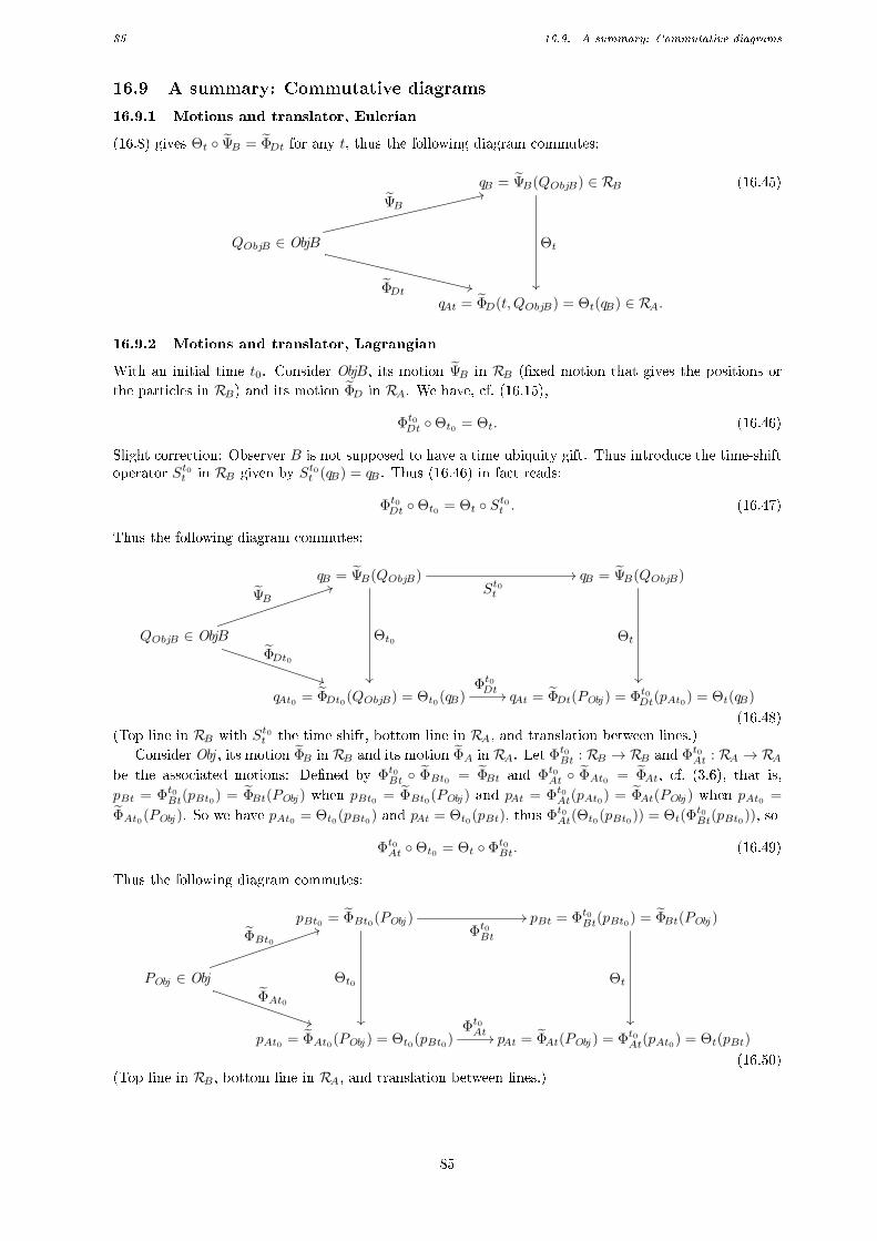
85 16.9. A summary: Commutative diagrams
16.9 A summary: Commutative diagrams
16.9.1 Motions and translator, Eulerian
(16.8) gives Θt ΨB = ΦDt for any t, thus the following diagram commutes:
qB = ΨB(QObjB) ∈ RB
Θt
QObjB ∈ ObjB
ΨB33
ΦDt ++
qAt = ΦD(t, QObjB) = Θt(qB) ∈ RA.
(16.45)
16.9.2 Motions and translator, Lagrangian
With an initial time t0. Consider ObjB, its motion ΨB in RB (xed motion that gives the positions or
the particles in RB) and its motion ΦD in RA. We have, cf. (16.15),
Φt0Dt Θt0 = Θt. (16.46)
Slight correction: Observer B is not supposed to have a time ubiquity gift. Thus introduce the time-shiftoperator St0t in RB given by St0t (qB) = qB . Thus (16.46) in fact reads:
Φt0Dt Θt0 = Θt St0t . (16.47)
Thus the following diagram commutes:
qB = ΨB(QObjB)
Θt0
St0t
// qB = ΨB(QObjB)
Θt
QObjB ∈ ObjB
ΨB44
ΦDt0
**
qAt0 = ΦDt0(QObjB) = Θt0(qB)Φt0Dt // qAt = ΦDt(PObj ) = Φt0Dt(pAt0) = Θt(qB)
(16.48)(Top line in RB with St0t the time shift, bottom line in RA, and translation between lines.)
Consider Obj , its motion ΦB in RB and its motion ΦA in RA. Let Φt0Bt : RB → RB and Φt0At : RA → RAbe the associated motions: Dened by Φt0Bt ΦBt0 = ΦBt and Φt0At ΦAt0 = ΦAt, cf. (3.6), that is,
pBt = Φt0Bt(pBt0) = ΦBt(PObj ) when pBt0 = ΦBt0(PObj ) and pAt = Φt0At(pAt0) = ΦAt(PObj ) when pAt0 =
ΦAt0(PObj ). So we have pAt0 = Θt0(pBt0) and pAt = Θt0(pBt), thus Φt0At(Θt0(pBt0)) = Θt(Φt0Bt(pBt0)), so
Φt0At Θt0 = Θt Φt0Bt. (16.49)
Thus the following diagram commutes:
pBt0 = ΦBt0(PObj )
Θt0
Φt0Bt
// pBt = Φt0Bt(pBt0) = ΦBt(PObj )
Θt
PObj ∈ Obj
ΦBt044
ΦAt0
**
pAt0 = ΦAt0(PObj ) = Θt0(pBt0)Φt0At // pAt = ΦAt(PObj ) = Φt0At(pAt0) = Θt(pBt)
(16.50)(Top line in RB , bottom line in RA, and translation between lines.)
85
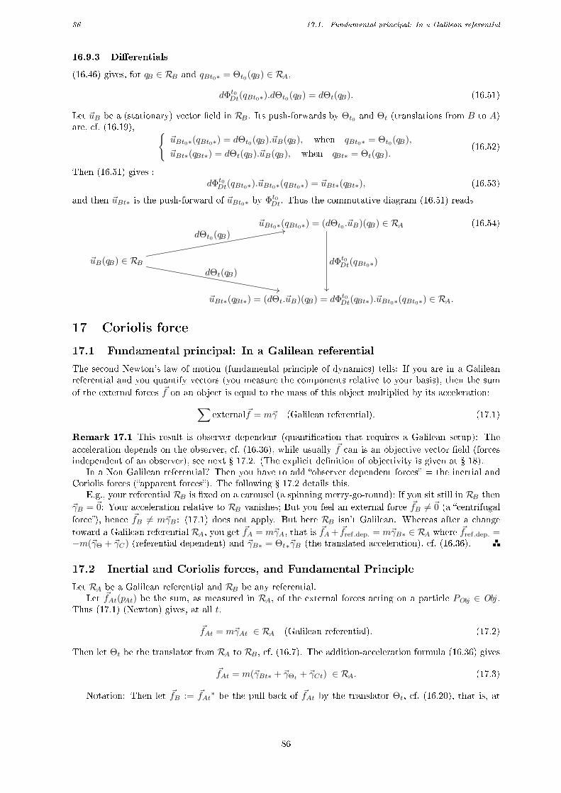
86 17.1. Fundamental principal: In a Galilean referential
16.9.3 Dierentials
(16.46) gives, for qB ∈ RB and qBt0∗ = Θt0(qB) ∈ RA,
dΦt0Dt(qBt0∗).dΘt0(qB) = dΘt(qB). (16.51)
Let ~uB be a (stationary) vector eld in RB . Its push-forwards by Θt0 and Θt (translations from B to A)are, cf. (16.19),
~uBt0∗(qBt0∗) = dΘt0(qB).~uB(qB), when qBt0∗ = Θt0(qB),
~uBt∗(qBt∗) = dΘt(qB).~uB(qB), when qBt∗ = Θt(qB).(16.52)
Then (16.51) gives :dΦt0Dt(qBt0∗).~uBt0∗(qBt0∗) = ~uBt∗(qBt∗), (16.53)
and then ~uBt∗ is the push-forward of ~uBt0∗ by Φt0Dt. Thus the commutative diagram (16.51) reads
~uBt0∗(qBt0∗) = (dΘt0 .~uB)(qB) ∈ RA
dΦt0Dt(qBt0∗)
~uB(qB) ∈ RB
dΘt0(qB)22
dΘt(qB)
,,
~uBt∗(qBt∗) = (dΘt.~uB)(qB) = dΦt0Dt(qBt∗).~uBt0∗(qBt0∗) ∈ RA.
(16.54)
17 Coriolis force
17.1 Fundamental principal: In a Galilean referential
The second Newton's law of motion (fundamental principle of dynamics) tells: If you are in a Galileanreferential and you quantify vectors (you measure the components relative to your basis), then the sum
of the external forces ~f on an object is equal to the mass of this object multiplied by its acceleration:∑external~f = m~γ (Galilean referential). (17.1)
Remark 17.1 This result is observer dependent (quantication that requires a Galilean setup): The
acceleration depends on the observer, cf. (16.36), while usually ~f can is an objective vector eld (forcesindependent of an observer), see next 17.2. (The explicit denition of objectivity is given at 18).
In a Non Galilean referential? Then you have to add observer dependent forces = the inertial andCoriolis forces (apparent forces). The following 17.2 details this.
E.g., your referential RB is xed on a carousel (a spinning merry-go-round); If you sit still in RB then
~γB = ~0: Your acceleration relative to RB vanishes; But you feel an external force ~fB 6= ~0 (a centrifugal
force), hence ~fB 6= m~γB : (17.1) does not apply. But here RB isn't Galilean. Whereas after a change
toward a Galilean referential RA, you get ~fA = m~γA, that is ~fA+ ~fref.dep. = m~γB∗ ∈ RA where ~fref.dep. =−m(~γΘ + ~γC) (referential dependent) and ~γB∗ = Θt∗~γB (the translated acceleration), cf. (16.36).
17.2 Inertial and Coriolis forces, and Fundamental Principle
Let RA be a Galilean referential and RB be any referential.Let ~fAt(pAt) be the sum, as measured in RA, of the external forces acting on a particle PObj ∈ Obj .
Thus (17.1) (Newton) gives, at all t,
~fAt = m~γAt ∈ RA (Galilean referential). (17.2)
Then let Θt be the translator from RA to RB , cf. (16.7). The addition-acceleration formula (16.36) gives
~fAt = m(~γBt∗ + ~γΘt + ~γCt) ∈ RA. (17.3)
Notation: Then let ~fB := ~fAt∗ be the pull-back of ~fAt by the translator Θt, cf. (16.20), that is, at
86
87 18.1. Covariant objectivity of a scalar function
any time t and with pAt = Θt(pBt),
~fBt(pBt) := dΘt(pBt)−1. ~fAt(pAt) ∈ RB , (17.4)
cf. (16.19)-(16.20). Thus (17.3) gives
~fBt(pBt) = mdΘt(pBt)−1.(~γBt∗(qAt) + ~γΘt(qAt) + ~γCt(qAt)) (17.5)
with the pull-backs notation, that is, ~γ∗(pBt) = dΘt(pBt)−1.~γ(qAt) (translation from A to B for vector
elds, cf. (16.20)). Thus
~fBt(pBt)−m~γΘt∗(pBt)−m~γCt∗(pBt) = m~γBt(pBt) ∈ RB . (17.6)
Denition 17.2 ~fit(pBt) = −m~γΘt
∗(pBt) = inertial force in RB at t,
~f∗Ct(pBt) = −m~γCt∗(pBt) = Coriolis force in RB at t.(17.7)
They are called ctitious forces (do not exist in a Galilean referential, are not objective).
Then (17.6) gives the fundamental principle in a non Galilean referential:
~fBt(pBt) + ~fit(pBt) + ~fCt(pBt) = m~γBt(pBt) (non Galilean referential). (17.8)
See e.g. villemin.gerard.free.fr/Scienmod/Coriolis.htm,planet-terre.ens-lyon.fr/article/force-de-coriolis.xml.
18 Objectivities
Framework of 16 (classical mechanics: The time scale is the same for all users).The goal is to give an objective expression of the laws of mechanics (observer independent), so that
two observers, quantifying relative to their referentials, will obtain results which they can communicateto each other (thanks to the translator).
Illustration: observer A chooses a referential RA = (OA, ( ~Ai)) xed on the Sun with ( ~Ai) a Euclidean
basis in foot, observer B chooses a referential RB = (OB , ( ~Bi)) xed on the Earth with ( ~Bi) a Euclideanbasis in meter, and Θt : RB → RA is the translator cf. (16.8).
Remark: The functions involved are Eulerian functions (objectivity cannot depend on the choice ofan initial time t0 which depends on an observer); If Lagrangian associated expressions are needed, theyare deduced a posteriori.
18.1 Covariant objectivity of a scalar function
Let f be a Eulerian scalar function corresponding to a physical quantity (e.g., temperature).The observers A and B describe f in their referential as being the functions fA :
R×RA → R(t, pA) → fA(t, pA)
and fB :
R×RB → R
(t, pB) → fB(t, pB)
. At t xed, let fAt(p) := fA(t, p) and
fBt(p) := fB(t, p).
Denition 18.1 The physical quantity f is objective covariant i, for all referentials RA and RB andfor all t,
fAt = Θt∗fBt = push-forward by Θt, cf. (10.5), (18.1)
that is,fAt(pAt) = fBt(pBt) when pAt = Θt(pBt). (18.2)
Or i fBt is the pull-back of fAt by Θt, cf. (10.10), that is, fBt = Θt∗fAt.
And then fA and fB are denoted f .
87
88 18.2. Covariant objectivity of a vector eld
18.2 Covariant objectivity of a vector eld
Let ~w be a Eulerian vector valued function corresponding to a physical quantity (e.g., a force).The observers A and B describe ~w in their referential as being the functions ~wA :
R×RA → ~Rn
(t, pA) → ~wA(t, pA)
and ~wB :
R×RB → ~Rn
(t, pB) → ~wB(t, pB)
. At t xed, let ~wAt(p) := ~wA(t, p) and
~wBt(p) := ~wB(t, p).
Denition 18.2 The physical quantity ~w is objective covariant i, for all referentials RA and RB andfor all t,
~wAt = Θt∗ ~wBt = push-forward by Θt, cf. (10.28) (18.3)
that is,~wAt(pAt) = dΘt(pBt). ~wBt(pBt) when pAt = Θt(pBt). (18.4)
Or i ~wBt is the pull-back of ~wAt by Θt, cf. (10.35), that is, ~wBt = Θt∗ ~wAt.
And then ~wA and ~wB are denoted ~w.
Example 18.3 Fundamental counter-example: A (Eulerian) velocity eld is not objective, cf. (16.27),because of the drive velocity ~vΘ = ~vD 6= ~0 in general. Neither is a (Eulerian) acceleration eld, cf. (16.36).In fact: An objective quantity is independent of a motion.
Example 18.4 The eld of gravitational forces ~g is objective.Remark: Compare ~gAt = m~γAt in a Galilean referential, cf. (17.1), and ~gBt + ~fit + ~fCt = m~γBt in a
non Galilean referential, cf 17: ~g is objective, so ~gAt(pAt) = dΘt(pBt).~gBt(pBt), but the acceleration ~γis not objective.
18.3 Isometric objectivity and Frame Invariance Principle
This manuscript is not intended to describe isometric objectivity:Isometric objectivity is the framework in which the principle of material frame-indierence (frame
invariance principle) is settled: Rigid body motions should not aect the stress constitutive law of amaterial. E.g., TruesdellNoll [19] p. 41:
Constitutive equations must be invariant under changes of frame of reference.
Or Germain [9] :
Axiom of power of internal forces. The virtual power of the "internal forces" acting on asystem S for a given virtual motion is an objective quantity; i.e., it has the same value whatever be the
frame in which the motion is observed.
NB: Both of these armations are limited to isometric changes of frame (the same metric for all), asTruesdellNoll [19] page 42-43 explain.
NB: The isometric objectivity (dened by one observer) has nothing to do with the covariant objec-tivity (relation between two observers). The isometric objectivity is an intra-referential concept, whichconcerns one observer who dened his Euclidean dot product (to give a meaning to a rigid body motion)and who looks at change of orthonormal bases to validate a constitutive law.
If we want to interpret isometric objectivity in the covariant objectivity setting, then Isometricobjectivity corresponds to a dictatorial management: One observer, e.g. A with his Euclidean referentialRA based on the English the foot, imposes his unit of length (the foot) to all other users (isometry);And only a change of orthonormal bases is allowed. This is a subjective approach: An English observer(foot) and an French observer (meter) cannot work together (they don't use the same metric).
Moreover, isometric objectivity leads to despise the dierence between covariance and contravari-ance, because of the uncontrolled generalized use of the Riesz representation theorem, see e.g. C.3and T.2, and leads to the misunderstanding of the Lie derivative of order 2 tensors (Jaumann, Trues-dell, Oldroyd, lower-Maxwell, upper-Maxwell...).
Remark 18.5 Marsden et Hughes [12] p. 8 use the same setting at rst. But, pages 22 and 163, they saythat a good modelization has to be covariant objective; And they do propose a covariant modeliza-tion for elasticity at 3.3, without mixing linear forms (covariant vectors) and vectors (contravariantvectors). (They use metrics but pay attention to the use of the Riesz representation theorem.)
88
89 18.4. Objectivity of dierential forms
18.4 Objectivity of dierential forms
A dierential form acts on vector elds, and the objectivity of a dierential form is deduced from theprevious .
Let α be a (Eulerian) dierential form corresponding to a physical quantity. The observers A andB describe α as being the functions αA : R×RA → RA and αB : R×RB → RB .
Denition 18.6 The physical quantity α is objective covariante i, for all referentials RA and RB andfor all t,
αAt = Θt∗αBt = push-forward by Θt, cf. (10.28) (18.5)
that is,αAt(pAt) = αBt(pBt).dΘt(pBt)
−1 when pAt = Θt(pBt). (18.6)
Or i αBt is the pull-back of αAt by Θt, that is, αBt = Θt∗αAt.
And then αA and αB are denoted α.
Thus, if ~w is an objective vector eld and it α is an objective dierential form, then the scalar functionα.~w is objective:
αAt(pAt). ~wAt(pAt) = αBt(pBt). ~wBt(pBt), (18.7)
since αAt(pAt). ~wAt(pAt) = (αBt(pBt).dΘt(pBt)−1).(dΘt(pBt). ~wBt(pBt)) = αBt(pBt). ~wBt(pBt). Matrix
expression. With proposition 16.12 and (16.44), we get: If α is objective, then
[αAt(pAt)]| ~B = [αBt(pBt)]| ~A.[P(pAt)]| ~A, i.e. [α]| ~B = [α]| ~A.P. (18.8)
Remark 18.7 (18.8) also reads [α]T| ~B = PT .[α]T| ~A, and one of the traps of isometric objectivity is that
P−1 = PT (change of orthonormal basis) so that [α]T| ~B = P−1.[α]T| ~A, cf. (18.8), equality which looks like
a contravariant expression, cf. (16.44),... except for the transposed!...: Thus the temptation is great toidentify a linear form with a vector...
But recall: It is impossible to identify a linear form with a vector: There is no natural canonicalisomorphism between a vector space and it dual space (the space of linear functionals), see T.2. Inparticular the Riesz representation theorem is not an identication: It is just a representation dependingon a measuring tool, cf. (C.11), that is, which depends on one observer.
Recall: Covariant objectivity respects the nature (vectorial or dierential) of the mathematical object.In particular a covariant objective framework does not use any inner dot product to begin with, andtherefore a linear form cannot be confused with a vector (there is no use of the Riesz's representationtheorem). E.g., the respect of covariance do not raise the problems seen at 13.2, and the problemat 15.8, problems due to the use of an inner dot product.
18.5 Objectivity of tensors
A tensor acts on both vector elds and dierential forms, and its objectivity is deduced from the previous .Let T be a (Eulerian) tensor corresponding to a physical quantity. The observers A and B describe
T as being the functions TA : R×RA → RA and TB : R×RB → RB .
Denition 18.8 The (Eulerian) physical quantity is objective covariante i, for all referentials RAand RB and for all t, TAt is the push-forward of TBt by Θt, cf. (14.7), that is, with pAt = Θt(pBt),
TAt(qAt)(., ..., .) = T (qB)(Θ∗t ., ...,Θ∗t .), i.e. TAt = Θt∗TBt
noted= TBt∗. (18.9)
And then TA and TB are denoted T .
Example 18.9 (Objectivity of a dierential d~w) Let ~w be an objective vector eld, seen as ~wAin RA and ~wB ∈ RB , thus ~wAt(pAt) = dΘt(pBt). ~wBt(pBt) when pAt = Θt(pBt), cf. (18.4).d~wAt(pAt).dΘt(pBt) = dΘt(pBt).d~wBt(pBt) + (d2Θt(pBt). ~wBt(pBt)), thus
d~wAt(pAt) = dΘt(pBt).d~wBt(pBt).dΘt(pBt)−1 + (d2Θt(pBt). ~wBt(pBt)).dΘt(pBt)
−1
6= dΘt(pBt).d~wBt(pBt).dΘt(pBt)−1 when d2Θt 6= 0.
(18.10)
Thus d~w is not objective in general (unless Θt is ane). However in classical mechanics, Θt is ane, and
89
90 18.6. Non objectivity of the velocities
thus d~w is considered to be objective when ~w is. And
d2 ~wAt(qAt).dΘt(qB).dΘt(qB) + d~wAt(qAt).d2Θt(qB)
= d3Θt(qB). ~wBt(qB) + 2 d2Θt(qB).d~wBt(qB) + dΘt(qB).d2 ~wBt(qB).(18.11)
Thusd2 ~w is objective i d2Θt = 0 (i.e. Θt is ane). (18.12)
18.6 Non objectivity of the velocities
18.6.1 Eulerian velocities
The velocity addition formal is, cf. (16.28), with ~vBt∗(pAt) = dΘt(pBt). ~w(pBt) when pAt = Θt(pBt),
~vAt(pAt) = ~vBt∗(pAt) + ~vDt(pAt)
6= ~vBt∗(pAt) when ~vDt(pAt) 6= ~0,(18.13)
thus a Eulerian velocity eld is not objective.
18.6.2 Lagrangian velocities
The Lagrangian velocities do not dene a vector eld, cf. 4.1.2. Thus asking about the objectivity ofLagrangian velocities is meaningless.
18.6.3 d~v is not objective
d~vBt is a eld of endomorphisms in RB . Its push-forward by Θt into RA is given by, cf. (14.23),
(d~vBt)∗(pAt) = dΘt(pBt).d~vBt(pBt).dΘt(pBt)−1, (18.14)
when pAt = Θt(pBt). And (~vAt − ~vDt)(pAt) = ~vBt∗(pAt) = dΘt(pBt).~vBt(pBt (velocity-addition formula),thus
d(~vAt − ~vDt)(pAt).dΘt(pBt) = d2Θt(pBt).~vBt(pBt) + dΘt(pBt).d~vBt(pBt). (18.15)
Hence, with (18.14),
d(~vAt − ~vDt)(pAt) = (d~vBt)∗(pAt) + (d2Θt(pBt).~vBt(pBt)).dΘt(pBt)−1. (18.16)
Thus d~vAt 6= Θt∗(d~vBt), hence d~v is not objective, even if d2Θt = 0 (because of ~vD). So, with ~uBt∗(pAt) =dΘt(pBt).~uBt we get in RA:
d(~vAt − ~vDt)(pAt).~uBt∗(pAt) = dΘt(pBt).d~vBt(pBt).~uBt(pBt) + d2Θt(pBt)(~uBt(pBt), ~vBt(pBt)). (18.17)
18.6.4 d~v is not isometric objective
Isometric objective implies• The use of the same Euclidean metric in RB and RA, i.e. (·, ·)a = (·, ·)b,• Φt0D is a solid body motion, i.e. dΦt0Dt
T.dΦt0Dt = I and Θt is ane (so d2Θt = 0 for all t).
Thus (18.16) givesd~vAt = d~vBt∗ + d~vDt. (18.18)
So d~vAt is not the push-forward d~vBt∗ = Θt∗(d~vBt) of ~vBt when d~vDt 6= 0, that is, when RB is notanimated with a uniform translation motion (e.g. for the Earth around the Sun). Thus d~v is not isometricobjective.
Remark 18.10 In classical mechanics courses, to establish that d~v isn't isometric objective, it is shownthat (change of coordinate system for dierentials of velocities for moving Euclidean referentials)
[d~vAt]| ~Bit∗ = Qt.[d~vAt]| ~A.Q−1t +Q′(t).Q−1
t , written [L]| ~Bit∗ = Q.[L]| ~A.QT +
•
Q.QT . (18.19)
Thus d~vAt(pAt) does not satisfy the change or coordinate rules for endomorphisms, because of•
Q.QT . Sod~v is not isometric objective.
90
91 18.7. The Lie derivative are covariant objective
Remark: (18.19) is not a change of (inter-)referential formula: (18.19) is given in one (intra-)referential
RA with a moving coordinate basis ( ~Bit∗) = (dΦt0Dt.~Ai) in RA, cf. (16.40):
~Bjt∗ = Pt. ~Aj =
n∑i=1
(Pt)ij~Ai, Pt = [(Pt)
ij ] = [Pt]| ~A, Qt = P−1
t . (18.20)
And with some t0 ∈ R, pAt = Φt0At(pAt0), and dΦt0A (t, pAt0) =noted F (t), we have, cf. (4.22),
d~vAt(pAt) = F ′(t).F (t)−1. (18.21)
And with (5.34) and Qt := P−1t we have
[F (t)]| ~Bit∗ = Q(t).[F (t)]| ~A, then [F ′(t)]| ~Bit∗ = Q′(t).[F (t)]| ~A +Q(t).[F ′(t)]| ~A (18.22)
Then (18.21) and (18.22) give
[d~vAt(pAt)]| ~Bit∗ = Q′(t).[F (t)]| ~A.[F (t)−1]| ~Bit∗ +Q(t).[F ′(t)]| ~A.[F (t)−1]| ~Bit∗
= Q′(t).[F (t)]| ~A.[F (t)]−1
| ~A.Q(t)−1 +Q(t).[F ′(t)]| ~A.[F (t)]−1
| ~A.Q(t)−1
= Q′(t).Q−1(t) +Q(t).[d~vAt(pAt)]| ~A.Q(t)−1,
(18.23)
that is, (18.19). And, with L = d~v cf. (4.22), this result is written [L]| ~Bit∗ =•
Q.QT + Q.[L]| ~A.QT . (And
with Q.QT = I, we get•
Q.QT + (•
Q.QT )T = 0, thus L+ LT is isometric objective.)
Exercice 18.11 Prove that d2~v is isometric objective.
Answer. (18.11) with ~vA − ~vD instead of ~wA and ~vB instead of ~wB give, in an isometric objective framework,
d2(~vAt − ~vDt)(pAt).(~uBt∗, ~wBt∗) = dΘt(pBt).d2~vBt(pBt)(~uB , ~wB). (18.24)
Thus if ΦDt is ane (which is the case of a rigid body motion) then d2~vDt = 0, cf. (9.6), and then d2~v is isometric
objective: d2~vAt(pAt).(~uBt∗, ~wBt∗) = dΘt(pBt).d2~vBt(pBt)(~uB , ~wB).
18.6.5 d~v + d~vT is isometric objective
Proposition 18.12 If Φt0D is a solid body motion then d~vt + d~vTt is isometric objective
d~vAt + d~vTAt = (d~vBt + d~vTBt)∗. (18.25)
(That is, the rate of deformation tensor is independent of a eventual added rigid motion.)
Proof. (18.18) gives d~vAt + d~vTAt = d(~vBt∗) + d~vDt + d(~vBt∗)T + d~vTDt, and Φt0D is a solid body motion, so
d~vDt + d~vTDt = 0, cf. (9.11), thus d~vAt + d~vTAt = d(~vBt∗) + d(~vBt∗)T .
And ~vBt∗(pAt) = dΘt(pBt).~vB(pBt) and pAt = Θt(pBt) and isometric objectivity (d2Θt = 0) gived(~vBt∗)(pAt).dΘt(pBt) = dΘt.d~vB(pBt) . Thus d(~vBt∗)(pAt) = dΘt.d~vB(pBt).dΘt
−1 = (d~vBt)∗(pAt).
Exercice 18.13 Prove that Ω = d~v−d~vT2 is not isometric objective.
Answer. (18.18) gives d~vTAt = d~vTBt∗+d~vTDt, thusd~vAt−d~vTAt
2=
d~vBt∗−d~vTBt∗2
+d~vDt−d~vTDt
26= d~vBt∗−d~vTBt∗
2, even if Φt0D
is a solid body motion (apart from a uniform translation).
18.7 The Lie derivative are covariant objective
The objectivity under concern is the covariant objectivity (no inner dot product is required to dene aLie derivative). The Lie derivatives are also called objective rates since they are covariant objective.
Framework of 16. We have the velocity-addition formula, cf. (16.28), that is, ~vAt = ~vBt∗+~vΘt in RA.
91
92 18.7. The Lie derivative are covariant objective
18.7.1 Scalar functions
Proposition 18.14 Let f be a covariant objective function, cf. (18.2). Then its Lie derivative L~vf iscovariant objective:
L~vAfA = Θ∗(L~vBfB), i.e. L~vAfA(t, pAt) = L~vBfB(t, pBt) when pAt = Θt(pBt), (18.26)
i.e., DfADt (t, pAt) = DfBDt (t, pBt).
But the dierential df and the partial derivative ∂f∂t are not objective in general.
Proof. Let pAt = pA(t) = ΦA(t, PObj ) and pBt = pB(t) = ΦB(t, PObj ), so pA(t) = Θ(t, pB(t)). (16.2) gives
L~vAfA(t, pAt) = DfADt (t, pAt) = ∂fA
∂t (t, pAt) + dfA(t, pAt).~vA(t, pAt). And L~vBfB(t, pBt) = DfBDt (t, pBt) =
∂fB∂t (t, pBt) + dfB(t, pBt).~vB(t, pBt).And, f being objective, (18.2) gives fB(t, pBt) = fA(t, pAt) = fA(t,Θ(t, pBt)).Thus ∂fB
∂t (t, pBt) = ∂fA∂t (t,ΘtpBt(t)) + dfA(t, pAt).~vΘt(pAt), and dfBt(pBt) = dfAt(pAt).dΘt(pBt).
Thus ∂fB∂t (t, pBt)+dfBt(pBt).~vBt(pBt) = ∂fA∂t (t, pAt)+dfAt(pAt).~vΘt(pAt)+dfAt(pAt).dΘt(pBt).~vBt(pBt) =
∂fA∂t (t, pAt) + dfAt(pAt).~vAt(pAt), since ~vΘt(pAt) + dΘt(pBt).~vBt(pBt) = ~vAt(pAt) is the velocity addictionformula (16.28).
18.7.2 Vector elds
Proposition 18.15 Let ~w be a covariant objective vector eld, cf. (18.4). Then its Lie derivative L~v ~wis covariant objective:
L~vA ~wA = Θ∗(L~vB ~wB), (18.27)
i.e., when pAt = Θt(pBt),L~vA ~wA(t, pAt) = dΘt(pBt).L~vB ~wB(t, pBt), (18.28)
i.e.,
(D~wADt
− d~vA. ~wA)(t, pAt) = dΘ(t, pBt).(D~wBDt
− d~vB . ~wB)(t, pBt), (18.29)
i.e.,
(∂ ~wA∂t
+ d~wA.~vA − d~vA. ~wA)(t, pAt) = dΘ(t, pBt).(∂ ~wB∂t
+ d~wB .~vB − d~vB . ~wB)(t, pBt). (18.30)
But the convected, Lie autonomous, partial, and material derivatives are not objective (recall thevelocity addition formula ~vAt−~vDt = ~vBt∗): We have
(d~wAt.(~vAt−~vDt))(pAt) = (dΘt.(d~wBt.~vBt) + (d2Θt. ~wBt).~vBt)(pBt), (18.31)
(d(~vAt−~vDt). ~wAt)(pAt) = (dΘt.(d~vBt. ~wBt) + (d2Θt.~vBt). ~wBt)(pBt), (18.32)
(d(~vAt−~vDt).(~vAt−~vDt))(pAt) = (dΘt.(d~vBt.~vBt) + d2Θt(~vBt, ~vBt))(pBt), (18.33)
L0(~vAt−~vDt) ~wAt(pAt) = dΘt(pBt).L0
~vBt~wBt(pBt), (18.34)
∂ ~wA∂t
(t, pAt) + L0~vD~wAt(pAt) = dΘt(pBt).
∂ ~wB∂t
(t, pBt), (18.35)
D~wADt
(t, pAt)− d~vDt. ~wAt(pAt) = dΘt.(pBt).D~wBDt
(t, pBt) + d2Θt(~vBt, ~wBt)(pBt), (18.36)
∂(~vA−~vD)
∂t(t, pAt) + L0
~vD(~vA−~vD)(t, pAt) = dΘt(pBt).
∂~vB∂t
(t, pBt). (18.37)
Proof. • ~wAt(Θt(pBt)) = dΘt(pBt). ~wBt(pBt) gives
d~wAt(pAt).dΘt(pBt) = d2Θt(pBt). ~wBt(pBt) + dΘt(pBt).d~wB(pBt), (18.38)
with dΘt(pBt).~vBt(pBt) = (~vAt−~vDt)(pAt) = ~vBt∗(pAt) (velocity-addition formula), thus
d~wAt(pAt).dΘt(pBt).~vBt(pBt) = (d2Θt(pBt).~vBt(pBt)). ~wBt(pBt) + dΘt(pBt).d~wBt(pBt).~vBt(pBt),
hence (18.31). In particular d~wAt(pAt).~vAt(pAt) 6= dΘt(pBt).(d~wBt(pBt).~vBt(pBt)) (the vector eld d~w.~v isnot objective).
92
93 18.8. Taylor expansions and ubiquity gift
• (~vAt−~vDt)(Θt(pBt)) = dΘt(pBt).~vBt(pBt) gives
d(~vAt−~vDt)(pAt).dΘt(pBt) = d2Θt(pBt).~vBt(pBt) + dΘt(pBt).d~vBt(pBt),
so, applied to ~wBt (resp. ~vBt), we get (18.32) (resp. (18.33)). Hence (18.34).
• If qAt = Θt(qB), then ~wA(t,Θ(t, qB)) = dΘ(t, qB). ~wB(t, qB), so, with ∂Θ∂t (t, qB) = ~vΘt(Θt(qB)), we get
∂ ~wA∂t
(t, qAt) + d~wAt(qAt).~vΘt(qAt) = d∂Θ
∂t(t, qB). ~wBt(qB) + dΘt(qB).
∂ ~wB∂t
(t, qB)
= (d~vΘt(qAt).dΘt(qB)). ~wBt(qB) + dΘt(qB).∂ ~wB∂t
(t, qB),
Thus (18.35) since ~vΘ = ~vD; Then with (18.31) we get (18.36).
• ~vB∗(t,Θ(t, qB)) = dΘ(t, qB).~vB(t, qB) gives
∂~vB∗∂t
(t, qAt) + d~vB∗(qAt).~vΘ(t, qAt) =∂dΘ
∂t(t, pBt).~vBt(pBt) + dΘ(t, pBt).
∂~vB∂t
(t, pBt)
= d~vΘt(pAt).dΘt(pBt).~vBt(pBt) + dΘ(t, pBt).∂~vB∂t
(t, pBt).
hence (18.37).
18.7.3 Tensors
Proposition 18.16 It T is an objective tensor, then:
L~vATA = Θ∗(L~vBTB). (18.39)
Proof. Corollary of (18.26) and (18.28) to get L~v(α.~w) = (L~vα). ~w + α.(L~v ~w); Then use L~v(t1 ⊗ t2) =(L~vt1)⊗ t2 + t1 ⊗ (L~vt2).
18.8 Taylor expansions and ubiquity gift
18.8.1 In Rn with ubiquity
Reminder:
f(t) = f(t0) + (t−t0) f ′(t0) +(t−t0)2
2f ′(t0)2 + o((t−t0)2). (18.40)
In particular f(t) = ~w(t, p(t)) gives
~w(t, p(t)) = ~w(t0, p(t0)) + (t−t0)D~w
Dt(t0, p(t0)) +
(t−t0)2
2
D~w
Dt(t0, p(t0))2 + o((t−t0)2) (18.41)
Problem : ~w(t, p(t)) is a vecteur at t at p(t) while ~w(t0, p(t0)) is a vecteur at t0 at p(t0), so (18.41)cannot be written
~w(t, p(t))−(~w(t0, p(t0)) + (t−t0)
D~w
Dt(t0, p(t0)) +
(t−t0)2
2
D~w
Dt(t0, p(t0))2
)= o((t−t0)2), (18.42)
since the left-hand side supposes the ubiquity gift.And in a non-planar manifold ~w(t, p(t)) ∈ Tp(t)Ω = the linear tangent space at p(t), whereas
~w(t0, p(t0)) ∈ Tp(t0)Ω = the linear tangent space at p(t0), and the tangent spaces are distinct at twodistinct points in general; Thus the left-hand side of (18.42) is meaningless.
In Rn the linear space ~Rnt and ~Rnt0 are identied, and (18.41) is well dened and very useful!
93
94 18.8. Taylor expansions and ubiquity gift
18.8.2 General case
By denition, cf. (15.8),
L~v ~w(t0, p(t0)) =dΦt0t (p(t0))−1. ~w(t, p(t))− ~w(t0, p(t0))
t− t0+ o(1). (18.43)
Thus,dΦt0t (p(t0))−1. ~w(t, p(t)) = ~w(t0, p(t0)) + (t−t0)L~v ~w(t0, p(t0)) + o(t−t0), (18.44)
or~w(t, p(t)) = dΦt0t (p(t0)).
(~w(t0, p(t0)) + (t−t0)L~v ~w(t0, p(t0)) + o(t−t0)
). (18.45)
This is the rst order Taylor expansion without ubiquity gift.
Interpretation: At rst order, the estimation of ~w(t, p(t)) is given by the push-forward
dΦt0t (pt0).(~w(t0, pt0) + (t−t0)L~v ~w(t0, pt0)
). And here the right and left members of (18.45) are at t
at p(t). And as for a usual Taylor expansion, to estimate the value at t at p(t), we take the value at t0
at p(t0), here(~w+ (t−t0)L~v ~w
)(t0, pt0), but now we push-forward this value to be at t at p(t) (we do not
have the ubiquity gift). And (18.45) is meaningful on a (non-planar) manifold.
Proposition 18.17 In Rn, with the gift of ubiquity, (18.45) gives (18.41) at rst order.
Proof. Let dΦt0(t, pt0) = F t0pt0 (t) and h = t−t0; And in Rn (5.41) gives F t0pt0 (t0+h) = It0 +h d~v(t0, pt0) +
o(h), so F t0pt0 (t0+h). ~Wpt0= ~Wpt0
+ h d~v(t0, pt0). ~Wpt0+ o(h). Thus (18.45) gives:
~w(t, pt) = (I + h d~v(t0, pt0) + o(h)).((~w + h
D~w
Dt− h d~v.~w)(t0, pt0) + o(h)
)= (~w + h d~v.~w + h
D~w
Dt− h d~v.~w)(t0, pt0) + o(h)
= ~w(t0, pt0) + hD~w
Dt(t0, pt0) + o(h),
which is (18.41).
Proposition 18.18 In Rn, at second order we have
~w(t, p(t)) = dΦt0t (pt0).((~w + hL~v ~w +
h2
2L~v(L~v ~w))(t0, pt0) + o(h2)
). (18.46)
So if the values ~w(t0, pt0), L~v ~w(t0, pt0) and L~v(L~v ~w)(t0, pt0) are known, then ~w(t, p(t)) is estimated at
second order thanks to the push-forward of (~w + hL~v ~w + h2
2 L~v(L~v ~w))(t0, pt0) by Φt0t .
Proof. Let dΦt0(t, pt0) = F t0pt0 (t) and h = t−t0; (5.41) gives F t0pt0 (t) = It0 +h d~v(t0, pt0) + h2
2 d~γ(t0, pt0) +
o(h2). Thus, omitting the reference to (t0, pt0) to lighten the writing,
dΦt0t (pt0).(~w + hL~v ~w +h2
2L~vL~v ~w + o(h2))
=(I + h d~v +
h2
2d(D~v
Dt) + o(h2)
).(~w + hL~v ~w +
h2
2L~vL~v ~w + o(h2)
) (18.47)
The h0 term is I.~w = ~w. The h term is L~v ~w + d~v.~w = D~wDt . The h
2 term is the sum of
• 1
2L~vL~v ~w =
1
2(D2 ~w
Dt2− 2 d~v.
D~w
Dt− D(d~v)
Dt.~w + d~v.d~v.~w), cf.(15.45),
• d~v.L~v ~w = d~v.D~w
Dt− d~v.d~v.~w =
1
2(2d~v.
D~w
Dt− 2d~v.d~v.~w),
• 1
2d(D~v
Dt). ~w =
1
2(D(d~v)
Dt.~w + d~v.d~v.~w), cf.(2.42).
And the sum gives D2 ~wDt2 .
Alternate proof: Let ~g(t) = dΦt0(t, pt0)−1. ~w(t, p(t)) when p(t) = Φt0(t, pt0). So L~v ~w(t0, p(t0)) =~g ′(t0), cf. (15.18). And D~w
Du (u, p(u)) = d~v(u, p(u)). ~w(u, p(u)) + F tu(pt).~g′(u), cf. (15.19).
Thus D2 ~wDu2 (u, p(u)) = D(d~v)
Du (u, p(u)). ~w(u, p(u)) + d~v(u, p(u)).D~wDu (u, p(u)) + d~v(u, p(u).F tu(pt).~g′(u) +
F tu(pt).~g′′(u). Thus D2 ~w
Dt2 (t, p(t)) = (D(d~v)Dt . ~w + d~v.D~wDt + d~v.L~v ~w)(t, p(t)) + ~g ′′(t). With (15.45) we get
~g ′′(t) = L~v(L~v ~w)(t, p(t)), cf. (15.45).
94
95
Part V
Appendix
The denitions, notations and results are detailed, so that no ambiguity is possible. (Some notations canbe nightmarish when not understood, or arrive like a bull in a china-shop, or misused.) In particular, allthe basic denitions and notations apply to solids, uids, thermodynamics, general relativity, chemistry...(the same mathematics applies to everyone).
A Classical and duality notations
A.1 Contravariant vector and basis
A.1.1 Contravariant vector
Let (E,+, .) =notedE be a real vector space (= a linear space on the eld R).
Denition A.1 An element ~x ∈ E is called a vector, or a contravariant vector.
A vector is a vector... For quantication purposes, a basis is introduced by an observer, and then avector is expressed in the chosen basis with a set of components. When a second basis is chosen, thesame vector is represented by a second set of components, the two set of components being linked by thecontravariant formula [~x]|~enew = P−1.[~x]|~eold , see (A.68); Hence the name contravariant vector due tothe use of the inverse of P .
A.1.2 Basis
Let ~e1, ..., ~en ∈ E. The vectors ~e1, ..., ~en are linearly independent i, for all λ, ..., λn ∈ R, the equality∑ni=1λi~ei = ~0 implies λi = 0 for all i = 1, ..., n. And the vectors ~e1, ..., ~en span E i, for all ~x ∈ E,
∃λ1, ..., λn ∈ R such that ~x =∑ni=1λi~ei. A basis in E is a nite set ~e1, ..., ~en ⊂ E made of linearly
independent vectors which span E, in which case the dimension of E is n.
A.1.3 Canonical basis
Consider the eld R and the Cartesian product ~Rn = R× ...× R, n times. The canonical basis is
~e1 = (1, 0, ..., 0), ..., ~en = (0, ..., 0, 1), (A.1)
with 0 the addition identity element used n−1 times, and 1 the multiplication identity element used once.
Remark A.2 The 3-D geometric space (we live in) has no canonical basis: What would the identityelement 1 mean? 1 meter? 1 foot? 1 light-year? And there is no intrinsic preferred direction todene ~e1.
A.1.4 Cartesian basis
(René Descartes 1596-1650.) Let n = 1, 2, 3, let Rn be the usual ane space (space of points), and let~Rn = (~Rn,+, .) be the usual real vector space of bipoint vectors with its usual algebraic operations.
Let p ∈ Rn, and let (~ei(p)) be a basis at p.
A Cartesian basis in ~Rn is a basis independent of p (the same at all p), and then (~ei(p)) =named(~ei).Example of a non Cartesian basis: The polar basis, see example 10.17 (polar coordinate system).And a Euclidean basis is a particular Cartesian basis described in B.1.
A.2 Representation of a vector relative to a basis
We give the classical notation, e.g. used by Arnold [3] and Germain [8], and the duality notation, e.g.used by Marsden and Hughes [12]. Both classical and duality notation are equally good, but if you haveany doubts about using duality notations, go back to the unambiguous classical notations.
95
96 A.3. Bilinear forms
Denition A.3 Let ~x ∈ E. Let (~ei) be a basis in E. The components of ~x relative to the basis (~ei) arethe n real numbers x1, ..., xn (classical notation) also named x1, ..., xn (duality notation) such that
~x = x1~e1 + ...+ xn~en︸ ︷︷ ︸clas.
= x1~e1 + ...+ xn~en︸ ︷︷ ︸dual
, i.e. [~x]|~e =
x1...xn
︸ ︷︷ ︸clas.
=
x1
...xn
︸ ︷︷ ︸dual
, (A.2)
[~x]|~e being the column matrix representing ~x relative to the basis (~ei). (Of course xi = xi for all i.) Andthe column matrix [~x]|~e is simply named [~x] if one chosen basis is implicitly used. With the sum sign:
~x =
n∑i=1
xi~ei︸ ︷︷ ︸clas.
=
n∑i=1
xi~ei︸ ︷︷ ︸dual
(=
n∑J=1
xJ~eJ =
n∑α=1
xα~eα). (A.3)
(The index in a summation is a dummy index, even if you do not write the sum sign∑
to follow Enstein'sconvention: ~x = xi~ei = xI~eI = xα~eα.)
Example A.4 ~R2 and ~x = 3~e1 + 4~e2 =∑2i=1 xi~ei =
∑2i=1 x
i~ei: We have x1=x1=3 and x2=x2=4 with
classical and duality notations. And [~x]|~e = 3[~e1]|~e+4[~e2]|~e =∑2i=1 xi[~ei]|~e =
∑2i=1 x
i[~ei]|~e. In particular,
with δij = δij = δij :=
= 1 if i=j
= 0 if i6=j
the Kronecker symbols,
~ej =
n∑i=1
δij~ei︸ ︷︷ ︸clas.
=
n∑i=1
δij~ei︸ ︷︷ ︸dual
, i.e. [~e1]|~e =
10...0
, ..., [~en]|~e =
0...01
, (A.4)
that is, relative to the basis ~ei, the components of ~ej are the δij with classical notations, i.e., and are the
δij with duality notations, for i = 1, ..., n. And the matrices [~ej ]|~e mimic the use of ~Rn = R× ...× R andits canonical basis.
Remark A.5 The column matrix [~x]|~e is also called a column vector. NB: A column vector is not avector, but just a matrix (a collection of real numbers). See the change of basis formula (A.68) wherethe same vector is represented by two column vectors (two column matrices).
A.3 Bilinear forms
LetA andB be vector spaces and (F(A;B),+, .) =noted F(A;B) be the usual real vector space of functionswith the internal addition (f, g)→ f+g dened by (f+g)(x) = f(x)+g(x) and the external multiplication(λ, f)→ λ.f dened by (λ.f)(x) = λ(f(x)), for all f, g ∈ F(A;B), x ∈ A, λ ∈ R. And λ.f =noted λf .
A.3.1 Denition
Denition A.6 Let E and F be vector spaces. A bilinear form on E × F is a function g(·, ·) :E × F → R(~u, ~w) → g(~u, ~w)
which is linear for each variable, i.e., g(·, ·) ∈ F(E×F ;R) satises g(~u1+λ~u2, ~w) =
g(~u1, ~w)+λg(~u2, ~w) and g(~u, ~w1 +λ~w2) = g(~u, ~w1)+λg(~u, ~w2) for all ~u, ~u1, ~u2 ∈ E, ~w, ~w1, ~w2 ∈ F , λ ∈ R.
Let L(E,F ;R) be the set of bilinear forms E×F → R: It is a vector space, sub-space of F(E×F ;R).
A.3.2 Inner dot product, and metric
Denition A.7 In a vector space E, an inner dot product (or inner product, or inner scalar product)is a bilinear form g(·, ·) : E × E → R which is symmetric, i.e. g(~u, ~w) = g(~w, ~u) for all ~u, ~w ∈ E, anddenite positive, i.e. g(~u, ~u) > 0 for all ~u 6= ~0. And then (for inner dot products)
g(·, ·) noted= (·, ·)g, and g(~u, ~w) = (~u, ~w)gnoted
= ~u •g ~wnoted
= ~u • ~w, (A.5)
the last notation if one inner dot product (·, ·)g is imposed by one observer to all observers (if it ispossible... which is not possible in general...). And the associated norm is the function ||.||g : E → R+
96
97 A.3. Bilinear forms
given by, for all ~u ∈ E,||~u||g =
√(~u, ~u)g. (A.6)
To prove that ||.||g is indeed a norm, we use the CauchySchwarz inequality:
∀~u,~v ∈ E, |(~u, ~w)g| ≤ ||~u||g||~w||g, (A.7)
which translates the property: The second order polynomial p(λ) = ||~u+λ~w||2g = (~u+λ~w, ~u+λ~w)g is nonnegative, which also gives: |(~u, ~w)g| = ||~u||g||~w||g i ~u// ~w.
Denition A.8 Two vectors ~u, ~w ∈ E are (·, ·)g-orthogonal i (~u, ~w)g = 0.
Denition A.9 With Rn our usual ane geometric space, n = 1, 2 or 3, and ~Rn = the usual associatedvector space made of bipoint vectors. Let Ω ⊂ Rn be open in Rn. A metric in Ω is a function g :
Ω → L(~Rn, ~Rn;R)
p → g(p)named
= gp
such that, at each p ∈ Ω, gp is an inner dot product in ~Rn. (That is, a metric
in Ω is a(
02
)tensor g in Ω s.t. gp is an inner dot product in ~Rn at each p ∈ Ω.)
A.3.3 Quantication: Matrices [gij ]
E and F are nite dimensional vector spaces, dimE = n, dimF = m, (~ai) is a basis in E and (~bi) is abasis in F .
Denition A.10 Let g ∈ L(E,F ;R). The components of g relative to the bases (~ai) and (~bi) are thenm reals
gij := g(~ai,~bj), (A.8)
and [g]|~a,~b = [gij ] i=1,...,nj=1,...,m
is the matrix of g relative to the bases (~ai) and (~bi).
Proposition A.11 A bilinear form g ∈ L(E,F,R) is known as soon as the nm scalars gij = g(~ai,~bj) areknown. Thus dimL(E,F ;R) = nm. And, for all (~u, ~w) ∈ E × S, we have g(~u, ~w) = ([~u]|~a)T .[g]|~a,~b.[~w]|~b(with usual matrix computation rules), i.e. with shortened notation when the bases are implicit:
g(~u, ~w) = [~u]T .[g].[~w] . (A.9)
Proof. Let bij ∈ L(E,F ;R) be dened by bij(~ak,~b`) = δikδj` (all the element the matrix [bij ]|~a,~b are zero
except the element at the intersection of row i and column j which is equal to 1). Then∑ij λijbij = 0
implies (∑ij λijbij)(~ak,
~b`) = 0 implies∑ij λijbij(~ak,
~b`) = 0, so λk` = 0, for all k, `, thus the bij are inde-
pendent. Then let g ∈ L(E,F ;R). We have g =∑ij g(~ai,~bj)bij (trivial), thus the bij span L(E,F ;R).
Example A.12 dimE = dimF = 2. [g]|~a,~b =
(1 20 3
)means g(~a1,~b1) = g11 = 1, g(~a1,~b2) = g12 = 2,
g(~a2,~b1) = g21 = 0, g(~a2,~b2) = g22 = 3. E.g., g12 = [~a1]T|~a.[g]|~a,~b.[~b2]|~b = ( 1 0 ) .
(1 20 3
).
(01
)= 2.
Exercice A.13 If g ∈ L(E,E;R), if (~ai) is a basis, if λ ∈ R∗, prove:
if ~bi = λ~ai ∀i ∈ [1, n]N, then [g]|~b = λ2[g]|~a. (A.10)
(A change of unit of measurement has a great inuence on the matrix of g.) And check:
g(~u, ~w) = [~u]T|~a.[g]|~a.[~w]|~a = [~u]T|~b.[g]|~b.[~w]|~b (A.11)
In particular if (·, ·)g is a Euclidean dot product then the length ||~u||g =√
[~u]T|~a.[g]|~a.[~w]|~a depends only
on the unit of measure used to dene (·, ·)g. Can also be checked with change of basis formulas.
Answer. g(~bi,~bj) = g(λ~ai, λ~aj) = λ2g(~ai,~aj) (bilinearity) reads [g]|~b = λ2[g]|~a.
Then ~u =∑ni=1uai~ai =
∑ni=1ubi
~bi =∑ni=1ubiλ~ai gives uai = λubi, idem wai = λwbi, thus [~u]T|~b.[g]|~b.[~w]|~b =
1λ
[~u]T|~a.λ2[g]|~a.
1λ
[~w]|~a = [~u]T|~a.[g]|~a.[~w]|~a.
Change of basis formulas: [~u]T|~b.[g]|~b.[~w]|~b = (P−1.[~u]|~a)T .(PT .[g]|~a.P ).(P−1.[~w]|~a) = [~u]T|~a.[g]|~a.[~w]|~a.
97
98 A.4. Linear maps
A.4 Linear maps
A.4.1 Denition
Denition A.14 Let E and F be vector spaces. A function L : E → F is linear i L(~u1 + λ~u2) =L(~u1) + λL(~u2) for all ~u1, ~u2 ∈ E and all λ ∈ R (distributivity type relation). And (distributivitynotation):
L(~u)noted
= L.~u, so L(~u1 + λ~u2) = L.(~u1 + λ~u2) = L.~u1 + λL.~u2. (A.12)
NB: This dot notation L.~u is not a matrix product: No bases have been introduced yet.
Let L(E;F ) be the set of linear maps E → F : It is a vector space, subspace of (F(E;F ),+, .).If F = E then a linear map L ∈ L(E;E) is called an endomorphism in E.
Vocabulary: Let Li(E;E) be the space of linear invertible linear maps. If E is a nite dimension vectorspace, dimE = n, then, in algebra, the set (Li(E;E), ) of linear maps equipped with the compositionrule is named GLn(E) = the linear group (it is indeed a group). And in elementary courses, the lineargroup GLn(Mn) refers to n ∗ n invertible matrices with the matrix product rule.
Exercice A.15 Let E = (E, ||.||E) and F = (F, ||.||F ) be Banach spaces, and let Lic(E;F ) be thespace of invertible linear continuous maps E → F , with its usual norm ||L|| = sup||~x||E=1 ||L.~x||F . Let
Z :
Lic(E;F ) → Lic(E;F )
L → L−1
. Prove dZ(L).M = −L−1 M L−1, for all M ∈ Lic(E;F ). (Remark:
In nite dimensions, a linear map is always continuous.)
Answer. We have to consider limh→0Z(L+hM)−Z(L)
h= limh→0
(L+hM)−1−L−1
h(=noted dZ(L).M if the limit
exists). With N = L−1.M we have L + hM = L(I + hN). Thus (L + hM)−1 = (I + hN)−1.L−1 = (I − hN +
o(h)).L−1 as soon as ||hN || < 1, i.e., h < 1||N|| , true as soon as h < 1
||L−1|| ||M|| since ||N || ≤ ||L−1|| ||M ||. Thus
(L+hM)−1−L−1 = L−1−hN.L−1 +o(h)−L−1 = h(−N.L−1 +o(1)), thus limh→0(L+hM)−1−L−1
h= −N.L−1.
A.4.2 Quantication: Matrices [Lij ] = [Lij ]
Let E and F be nite dimensional vector spaces (to be able to use matrix representations), dimE = n
and dimF = m. Let (~ai) be a basis in E and (~bi) be a basis in F .
Denition A.16 The components of a linear map L ∈ L(E;F ) relative to the bases (~ai) and (~bi) arethe nm reals named Lij (classical notation), or L
ij (duality notation), dened by: For all i, j = 1, ..., n,
the reals Lij = Lij are the components of the vectors L.~aj relative to the basis (~bi). That is:clas. : L.~aj =
m∑i=1
Lij~bi,
dual L.~aj =
m∑i=1
Lij~bi,
so [L.~aj ]|~bclas.=
L1j
...Lmj
dual=
L1j
...Lmj
. (A.13)
And
[L]|~a,~bclas.= [Lij ] i=1,...,m
j=1,...,n
dual= [Lij ] i=1,...,m
j=1,...,n(A.14)
is the matrix of L relative to the bases (~ai) and (~bi). In particular [L.~aj ]|~b is the j-th column of [L]|~a,~b.
Particular case: If E = F (so L is an endomorphism) and if (~bi) = (~ai) then [L]|~a,~a =named[L]|~a.
Example A.17 n = m = 2. [L]|~a,~b =
(1 20 3
)means L.~a1 = ~b1 and L.~a2 = 2~b1 + 3~b2 (column reading).
Thus, L11=L11=1, L12=L1
2=2, L21=L21=0, L22=L2
2=3, with classical and duality notations.
And L being linear, for all ~u ∈ E, ~u =∑nj=1uj~aj =
∑nj=1u
j~aj , we get, thanks to linearity,
L.~u =
m∑i=1
n∑j=1
Lijuj~bi︸ ︷︷ ︸clas.
=
m∑i=1
n∑j=1
Lijuj~bi︸ ︷︷ ︸
dual
, i.e. [L.~u]|~b = [L]|~a,~b.[~u]|~a . (A.15)
Shortened notation: [L.~u] = [L].[~u] (implicit bases).
98
99 A.5. Transposed matrix
Proposition A.18 A linear map L ∈ L(E;F ) is known i the n vectors L(~aj) are known. Thusdim(L(E;F )) = nm.
Proof. ~u ∈ E and ~u =∑ni=1ui~ai give L(~u) =
∑ni=1uiL(~ai), thanks to the linearity of L. Thus L is known
i all the n vectors L(~aj), j = 1, ..., n, are known. And a vector L(~aj) is known i its m components Lijare known. (Use duality notations if you prefer.)
Exercice A.19 If L ∈ L(E;E) (endomorphism), if (~ai) is a basis, prove:
if λ ∈ R∗ and if ~bi = λ~ai ∀i ∈ [1, n]N, then [L]|~b = [L]|~a : (A.16)
A change of unit has not inuence on the matrix of an endomorphism. Check this result with the changeof basis formulas To compare with (A.10): Covariance and contravariance should not be confused.
Answer. Let L.~aj =∑ni=1Lij~ai. Then L.
~bj = L.(λ~aj) = λL.~aj = λ∑ni=1Lij~ai = λ
∑ni=1Lij
~biλ
=∑ni=1Lij
~bi.
Change of basis formula: [L]|~b = P−1.[L]|~a.P with P = λI here.
A.5 Transposed matrix
The denition can be found in any elementary books, e.g., Strang [18]:
Denition A.20 Let M = [Mij ] i=1,...,mj=1,...,n
be an m ∗ n matrix. Its transposed is the n ∗m matrix MT =
[(MT )ij ] i=1,...,nj=1,...,m
dened by (MT )ij := Mji (exchange rows and columns).
E.g., if M =
(1 23 4
)then MT =
(1 32 4
); E.g., (MT )12=M21=3.
A.6 The transposed endomorphisms of an endomorphism
Let (E, (·, ·)g) be a nite dimensional vector space equipped with an inner dot product g(·, ·) = (·, ·)g.
A.6.1 Denition (requires an inner dot product)
Denition A.21 The transpose of an endomorphism L ∈ L(E;E) relative to the inner dot product (·, ·)gis the endomorphism LTg ∈ L(E;E) dened by
∀~x, ~y ∈ E, (LTg (~y), ~x)g = (~y, L(~x))g, written (LTg .~y, ~x)g = (~y, L.~x)g, (A.17)
the dot notations since LTg and L are linear maps (it is not a matrix product: No basis has been introduced
yet). This denes the map (.)Tg :
L(E;E) → L(E;E)
L → LTg
.
We immediately get (LTg )Tg = L.
If (·, ·)g is imposed and non ambiguous, then LTg =named LT .
Remark A.22 If E is nite dimensional, then the existence and uniqueness of LTg is proved thanks to
a basis in E. If E innite dimensional and (E, (·, ·)g) a Hilbert space, and if L is continuous, then LTgexists and is unique by application of the Riesz representation theorem.
A.6.2 Quantication with bases
Relative to a basis (~ei) E, (A.17) gives [~x]T .[g].[LTg ].[~y] = [L.~x]T .[g].[~y] = [~x]T .[L]T .[g].[~y] for all ~x, ~y, thus
[g].[LT ] = [L]T .[g], i.e. [LT ] = [g]−1.[L]T .[g] . (A.18)
Full notation: [g]|~e.[LTg ]|~e = ([L]|~e)
T .[g]|~e, and [LTg ]|~e = [g]−1|~e .([L]|~e)
T .[g]|~e. I.e., with classical notations,
if g(~ei, ~ej) = gij , L.~ej =
n∑i=1
Lij~ei, LTg .~ej =
n∑i=1
(LTg )ij , (A.19)
99
100 A.6. The transposed endomorphisms of an endomorphism
i.e., if [g]|~e = [gij ], [L]|~e = [Lij ], [LTg ]|~e = [(LTg )ij ],
then
n∑k=1
gik(LTg )kj =
n∑k=1
Lki gkj and (LTg )ij =
n∑k,`=1
([g]−1)ikL`kg`j . (A.20)
(If (~ei) is a (·, ·)g-orthonormal basis then [g] = [δij ] and (LTg )ij = Lji.)
And, with duality notations, if L.~ej =∑ni=1L
ij~ei and L
Tg .~ej =
∑ni=1(LTg )ij , i.e., if [L]|~e = [Lij ] and
[LTg ]|~e = [(LTg )ij ], then
n∑k=1
gik(LTg )kj =
n∑k=1
Lki gkj and (LTg )ij =
n∑k,`=1
([g]−1)ikL`k g`j . (A.21)
Remark A.23 Warning: The last equation (A.21)2 is also written
(LTg )ij =
n∑k,`=1
gikL`k g`j when ([g]~e)−1 = [gij ]
−1 noted= [gij ]. (A.22)
Don't be fooled by the notation [gij ] here: It is not a duality notation here: It is just the inverse matrix
of the matrix [gij ]. E.g., if [g]~e = [gij ] =
(1 00 2
)then [gij ] := ([g]~e)
−1 =
(1 00 1
2
). Return to the
classical notations if in doubt. (To understand the origin of the notation gij , go to A.12.7: gij is relatedwith an inner dot product in E∗.
Exercice A.24 In ~R2, let (~e1, ~e2) be a basis. Let L ∈ L( ~R2; ~R2) be dened by [L]|~e =
(0 11 0
). Find
two inner dot products (·, ·)g and (·, ·)h in ~R2 such that LTg 6= LTh (a transposed endomorphism is notunique: It is not intrinsic to L since it depends on a choice of an inner dot product).
Answer. Calculations with (A.18):
Choose (·, ·)g given by [g]|~e =
(1 00 1
)= [I]. Thus [LTg ]|~e = [I].[L]|~e.[I] =
(0 11 0
); So LTg = L.
Choose (·, ·)h given by [h]|~e =
(1 00 2
). Thus [LTh ]|~e = [h]−1
|~e .[L]|~e.[h]|~e =
(0 212
0
); So LTh 6= L.
Thus LTh 6= LTg , e.g., ~e2 = LTg .~e1 6= LTh .~e1 = 12~e2.
Exercice A.25 Prove: If L is invertible then LTg is invertible, and (LTg )−1 = (L−1)Tg (called L−Tg ).
Answer. If the endomorphism LTg was not invertible, then ∃~y ∈ E s.t. ~y 6= ~0 and LTg .~y = 0, thus (~y, L.~x)g = 0,
for all ~x; And L being invertible we can choose ~x s.t.L.~x = ~y to get ||~y||g = 0, thus ~y = 0: Absurd since ~y 6= ~0.Thus LTg is invertible.
Then (LTg .(L−1)Tg .~x, ~y)g
(A.17)= ((L−1)Tg .~x, L.~y)g
(A.17)= (~x, (L−1).L.~y)g = (~x, ~y)g = (I.~x, ~y)g = (LTg .(L
Tg )−1.~x, ~y)g,
true ∀~x, ~y, thus LTg .(L−1)Tg = LTg .(LTg )−1, thus (L−1)Tg = (LTg )−1.
Exercice A.26 Special case of proportional inner dot products: Let λ > 0 and suppose (·, ·)a = λ2(·, ·)b.Prove: LTa = LTb : Two proportional inner dot products give the same transposed endomorphism.
Answer. (LTb .~y, ~x)b = (~y, L.~x)b = λ2(L.~y, ~x)a = λ2(LTa .~y, ~x)a = (LTa .~y, ~x)b, for all ~x, ~y, so LTb = LTa .
A.6.3 Symmetric endomorphism
Denition A.27 An endomorphism L ∈ L(E;E) is (·, ·)g-symmetric i LTg = L, that is,
L (·, ·)g-symmetric ⇐⇒ LTg = L ⇐⇒ (L.~x, ~y)g = (~x, L.~y)g, ∀~x, ~y ∈ E. (A.23)
Remark A.28 The symmetric character of an endomorphism L is not intrinsic to the endomorphism:It depends on (·, ·)g; See exercise A.24: LTg is (·, ·)g-symmetric, and LTh isn't (·, ·)h-symmetric.
Quantication: L ∈ L(E;E) is (·, ·)g-symmetric i LTg = L i [LTg ]|~e = [L]|~e, i.e. i [g]−1|~e .[L]T|~e.[g]|~e =
[L]|~e cf. (A.18), i.e. i [L]T|~e.[g]|~e = [g]|~e.[L]|~e, for all basis (~ei). E.g., with exercise A.24 and (·, ·)h, we have
[L]T|~e.[h]|~e =
(0 21 0
)6= [h]|~e.[L]|~e =
(0 12 0
), thus L is not (·, ·)h symmetric.
Particular case (~ei) is a (·, ·)g-orthonormal basis: L ∈ L(E;E) is (·, ·)g-symmetric i [L]T|~e = [L]|~e.
100
101 A.7. The transposed of a linear map
A.7 The transposed of a linear map
A.7.1 Denition (needs two inner dot products)
E and F are nite dimensional vector spaces, (·, ·)g and (·, ·)h are an inner dot products in E and F .(The case E = F and (·, ·)g = (·, ·)h is treated in A.6.)
Let L ∈ L(E;F ). E.g.: L = dΦt0t (P ) : ~Rnt0 → ~Rnt is the deformation gradient, cf. (5.2), and (·, ·)g is theinner dot product chosen by the observer who made the measurements at t0 (e.g. the foot built Euclideandot product), and (·, ·)h is the inner dot product chosen by the observer who makes the measurementsat t (e.g. the meter built Euclidean dot product).
Denition A.29 The transposed of L ∈ L(E;F ) relative to (·, ·)g and (·, ·)h is the linear map LTgh ∈L(F ;E) dened by, for all (~x, ~y) ∈ E × F ,
(LTgh(~y), ~x)g = (~y, L(~x))h, written (LTgh.~y, ~x)g = (~y, L.~x)h, (A.24)
the dot notation since LTgh and L are linear maps (it is not a matrix product: No bases have been
introduced yet). This denes the map (.)Tgh :
L(E;F ) → L(F ;E)
L → LTgh
.
We immediately get (LTgh)Thg = L..
If F = E and (·, ·)h = (·, ·)g then LTgh = LTg , see A.6.
A.7.2 Quantication with bases
Let (~ai) be a basis in E, (~bi) be a basis in F . (A.24) gives (LTgh.~bj ,~ai)g = (~bj , L.~ai)h,
i.e., [~ai]T|~a.[g]|~a.[L
Tgh]|~b,~a.[
~bj ]|~b = ([L.~ai]|~b)T .[h]|~b.[
~bj ]|~b = [~ai]T|~a.([L]|~a,~b)
T .[h]|~b.[~bj ]|~b for all i, j, thus,
[g]|~a.[LTgh]|~b,~a = ([L]|~a,~b)
T .[h]|~b and [LTgh]|~b,~a = [g]−1|~a .([L]|~a,~b)
T .[h]|~b. Shortened notations:
[g].[LTgh] = [L]T .[h], i.e. [LTgh] = [g]−1.[L]T .[h] , (A.25)
With components, classical and duality notations:
g(~ai,~aj) = gij , h(~bi,~bj) = hij , [g]|~a = [gij ], [h]|~b = [hij ]
clas. : L.~aj =
m∑i=1
Lij~bi, LTgh.~bj =
n∑i=1
(LTgh)ij~ai, [L]|~a,~b = [Lij ], [LTgh]|~b,~a = [(LTgh)ij ],
dual : L.~aj =
m∑i=1
Lij~bi, LTgh.~bj =
n∑i=1
(LTgh)ij~ai, [L]|~a,~b = [Lij ], [LTgh]|~b,~a = [(LTgh)ij ],
(A.26)
gives, for (A.25)1,n∑k=1
gik(LTgh)kj =
m∑k=1
Lki hkj︸ ︷︷ ︸clas.
=
n∑k=1
gik(LTgh)kj =
m∑k=1
Lki hkj︸ ︷︷ ︸dual
, (A.27)
and, for (A.25)2,
(LTgh)ij =
n∑k=1
m∑`=1
([g]−1)ikL`kh`j︸ ︷︷ ︸clas.
= (LTgh)ij =
n∑k=1
m∑`=1
gikL`k h`j︸ ︷︷ ︸dual
when [gij ] := ([g]~e)−1. (A.28)
Exercice A.30 Prove: If L is invertible then (LTgh)−1 = (L−1)Thg.
Answer. (LTgh.(L−1)Thg.~x, ~y)g = ((L−1)Thg.~x, L.~y)h = (~x, L−1.L.~y)g = (~x, ~y)g = (LTgh.(L
Tgh)−1.~x, ~y)g, true ∀~x, ~y.
A.7.3 Deformation gradient symmetric: Absurd
The symmetry of a linear map L ∈ L(E;F ) is a nonsense if F 6= E.Application: The gradient of deformation F t0t (pt0) = dΦt0t (pt0) ∈ L(Tpt0 (Ωt0);Tpt(Ωt)) cannot be
symmetric since F t0t (pt0)T = (F t0t )T (pt) ∈ L(Tpt(Ωt);Tpt0 (Ωt0)). (Reason for the introduction of the sec-ond PiolaKirchho tensor ∈ L(Tpt0 (Ωt0);Tpt0 (Ωt0)): Symmetric, see MarsdenHughes [12] or M.3.2.)
101
102 A.8. Dual basis
A.7.4 Isometry
Denition A.31 A linear map L ∈ L(E;F ) is an isometry relative to (·, ·)g and (·, ·)h i
∀~x, ~y ∈ E, (L.~x, L.~y)h = (~x, ~y)g, i.e. LTgh L = IE (identity in E). (A.29)
In particular, if L is an isometry and (~ei) is a (·, ·)g-orthonormal basis, then (L.~ei) is a (·, ·)h-orthonormal basis, since (L.~ei, L.~ej)h = (~ei, ~ej)g = δij for all i, j.
In particular, an endomorphism L ∈ L(E;E) is a (·, ·)g-isometry i
∀~x, ~y ∈ E, (L.~x, L.~y)g = (~x, ~y)g, i.e. LTg L = I. (A.30)
Thus, if L is an isometry and (~ei) is a (·, ·)g-orthonormal basis, then (L.~ei) is a (·, ·)g-orthonormal basis.
Exercice A.32 Let E = R3 be the usual ane space and E = ~R3 the usual associated vector space;
Let (·, ·)g be an inner dot product in ~R3. Denition: A distance-preserving function f : R3 → R3 is a
function s.t. ||−−−−−→f(p)f(q)||g = ||−→pq||g for all p, q ∈ R3. Prove: If f is a distance-preserving function, then fis ane, and df is an isometry.
Answer. Let O ∈ R3 (an origin), and consider the vectorial associated function ~f : ~x =−→Op ∈ ~R3 →
~f(~x) :=−−−−−−→f(O)f(p). Let ~y =
−→Oq. Then 2(~f(~x), ~f(~y))g = ||~f(~x)||2g + ||~f(~y)||2g − ||~f(~x) − ~f(~y)||2g = ||−−−−−−→f(O)f(p)||2g +
||−−−−−−→f(O)f(q)||2g − ||−−−−−→f(q)f(p)||2g = ||−→Op||2g + ||−→Oq||2g − ||−→qp||2g = ||~x||2g + ||~y||2g − ||~x − ~y||2g = 2(~x, ~y)g, for all ~x, ~y, thus
~f is an isometry, cf. (A.30). Thus, if (~ei) is a (·, ·)g-orthonormal basis,then (~f(~ei)) is also a (·, ·)g-orthonormal
basis. Thus ~f(~x) =∑ni=1(~f(~x), ~f(~ei))g ~f(~ei) =
∑ni=1(~x,~ei)g ~f(~ei) =
∑ni=1xi
~f(~ei) when ~x =∑ni=1xi~ei, thus
~f(~x+λ~y) =∑ni=1(xi+λyi)~f(~ei) = ~f(~x)+λ~f(~y), thus ~f is linear; Thus d~f(~x) = ~f = df(~x) =noted df (independent
of ~x), thus ~f = df (= d~f) is an isometry and f is ane: f(p) = f(O)+−−−−−−→f(O)f(p) = f(O)+~f(
−→Op) = f(O)+d~f.
−→Op.
A.8 Dual basis
A.8.1 Linear forms: Covariant vectors
With F = R in the denition A.14, we get
Denition A.33 The set E∗ := L(E;R) of linear scalar valued functions is called the dual of E:
E∗ := L(E;R) = the dual of E. (A.31)
And a linear scalar valued function ` ∈ E∗ is called a linear form.
(More precisely, E∗ is the algebraic dual, the topological dual being, if E is a Banach space, the subsetof continuous linear forms; Recall: If E is nite dimensional, all norms are equivalent and any linear formis continuous.)
And (A.12) gives: If ` ∈ E∗ = L(E;R), then
∀~u ∈ E, `(~u)noted
= `.~u. (A.32)
`(~u) is also written 〈`, ~u〉E∗,E where 〈., .〉E∗,E is the duality bracket: It is not an inner dot product (` /∈ E),it is a duality product, the calculation `(~u) = `.~u = 〈`, ~u〉E∗,E being called a covariant calculation, theresult being independent of an observer.
Denition A.34 A linear form ` in E∗ is also called a covariant vector; Co-variant refers to:1- The action of a function on a vector, cf. (A.32) (covariant calculation), and2- The change of coordinate formula [`]new = [`]|old.P , see (A.68) (covariant formula).
NB: E∗ being a vector space, an element ` ∈ E∗ is indeed a vector. But E∗ has no existence if E hasnot been specied rst, a covariant vector ` ∈ E∗ being a function on E: It can't be confused with avector in E since there is no natural canonical isomorphism between E and E∗.
Remark A.35 MisnerThorneWheeler [14], box 2.1, insist: Without it [the distinction between co-variance and contravariance], one cannot know whether a vector is meant or the very dierent objectthat is a linear form.
Interpretation of a linear form (a covariant vector): It answers the question: What does a functionE → R do? Answer: Like any function, it gives values to vectors: `(~u) = the value of ~u through `.
102
103 A.8. Dual basis
A.8.2 Covariant dual basis (the functions which give the components of a vector)
Notation: If ~u1, ..., ~uk are k vectors in E, then Vect~u1, ..., ~uk := the vector space spanned by ~u1, ..., ~uk.
Denition A.36 Let (~ei)i=1,...,n be a basis in E (nite dimensional). Let i ∈ [1, n]N. The scalarprojection on Vect~ei parallel to Vect~e1, ..., ~ei−1, ~ei+1, ..., ~en is the linear form named πei ∈ E∗ withthe classical notation, and named ei ∈ E∗ with the duality notation, dened by, for all i, j,
clas. : πei(~ej) = δij , written πei.~ej = δij ,
dual : ei(~ej) = δij , written ei.~ej = δij ,(A.33)
the dot notations since πei = ei is linear. Drawing.
Proposition A.37 and denition of the dual basis. (πei)i=1,...,n = (ei)i=1,...,n is a basis in E∗, called
the covariant dual basis of the basis (~ei), or, simply, the dual basis of the basis (~ei) (in this manuscript).
Proof. If∑ni=1λiπei = 0, then (
∑ni=1λiπei)(~ej) = 0 for all j, thus
∑ni=1λiπei(~ej) = 0 =
∑ni=1λiδij = λj
for all j, thus (πei)i=1,...,n is a family of n independent vectors in E∗; And dimE∗ = n, cf. prop. A.18,thus (πei)i=1,...,n is a basis in E∗. (You can use duality notations if you prefer.)
Thus, πei = ei being linear, if ~x =∑ni=1xi~ei =
∑ni=1x
i~ei (classical or duality notations), then (A.33)gives
πei(~x) = xi︸ ︷︷ ︸clas.
= ei(~x) = xi︸ ︷︷ ︸dual
(A.34)
So πei = ei is the linear function E → R that gives the i-th component of a vector ~x relative to thebasis (~ei). Or, with the linearity dot notation, πei.~x = xi and = ei.~x = xi.
Example A.38 Following example 1.1. The size of a child is represented on a wall by a bipoint vector ~u.And observer (e.g. René Descartes) chooses a unit of length through a bipoint vector which he names ~e.
And then denes a linear form πe : ~R→ R by πe.~e = 1. Thus πe is a measuring instrument, built from ~e,which gives the size s of the child relative to ~e: It gives s = πe(~u) = πe.~u, so ~u = (πe.~u)~e.
Exercice A.39 Let (~ai) and (~bi) be bases and let πai and πbi be the dual bases. Let λ 6= 0. Prove:
If ∀i = 1, ..., n, ~bi = λ~ai, then ∀i = 1, ..., n, πbi =1
λπai. (A.35)
(With duality notations, bi = 1λ a
i.)
Answer. πbi.~bj = δij = πai.~aj = πai.~bjλ
= 1λπai.~bj for all j (since πai is linear), thus πbi = 1
λπai, true for all i.
NB: The dual basis is independent of any inner dot product (no inner dot product (·, ·)g has beenintroduced). In particular, πei.~ej = ei.~ej is not an inner dot product between two vectors, becauseπei = ei (function) and ~ei (vector) do not belong to the same vector space. It means πei(~ej) = ei(~ej),cf. (A.32).
A.8.3 Example: aeronautical units
Example A.40 International aeronautical units: Horizontal length = nautical mile (NM), altitude =English foot (ft). Application: An air trac controller chooses the point O = the position of its control
tower, and a plane p is located thanks to the bipoint vector ~x =−→Op. And the trac controller chooses
~e1 = the vector of length 1 NM indicating the south (rst runway), ~e2 = the vector of length 1 NMindicating the southwest (second runway), ~e3 = the vector of length 1 ft indicating the vertical. Thushis referential is R = (O, (~e1, ~e2, ~e3)), and his dual basis (πe1, πe2, πe3) is dened by πei(~ej) = δij for
all i, j, cf. (A.33). He writes ~x =∑ni=1xi~ei ∈ ~Rn, so that x1 = πe1(~x) = the distance to the south in NM,
x2 = πe2(~x) = the distance to the southwest in NM, x3 = πe3(~x) = the altitude in ft. (If you prefer, withduality notations, πei=e
i and ~x =∑ni=1x
i~ei and xi = ei.~x.)
Here the basis (~ei) is not a Euclidean basis. This non Euclidean basis (~ei) is however vital if you takea plane. (A Euclidean basis is not essential to life...). See next remark A.41.
103
104 A.8. Dual basis
Remark A.41 The meter is the international unit for NASA that launched the Mars Climate Orbiterprobe; The foot is the international vertical unit for aviation; And for the Mars Climate Orbiter landingprocedure, NASA asked Lockheed Martin to do the computation. Result? The Mars Climate Orbiterspace probe burned in the Martian atmosphere because of λ ∼ 3 times too high a speed during thelanding procedure: One meter is λ ∼ 3 times one foot, and someone forgot it... Although everyoneused a Euclidean dot product... But not the same (one based on a meter, and one based on the foot).(Objectivity and covariance can be useful...)
A.8.4 Matrix representation of a linear map
Let ` ∈ E∗, let (~ei) be a basis: The components of ` are the n reals
`i := `(~ei) = `.~ei, and [`]|~e = ( `1 ... `n ) (row matrix) (A.36)
is the matrix of ` relative to the basis (~ei). In particular for the dual basis (πei) = (ei),
[πej ]|~e = [ej ]|~e = (0 ... 0 1︸︷︷︸jth position
0 ... 0) = [~ej ]T|~e (row matrix), (A.37)
And we get (usual representation of components with a basis), with classical and duality notations,
`clas.=
n∑i=1
`i πeidual=
n∑i=1
`i ei. (A.38)
Thus with ~x =∑ni=1xi~ei =
∑ni=1x
i~ei ∈ E, linearity gives, with classical and duality notations,
`.~x = [`]|~e.[~x]|~e =
n∑i=1
`ixi =
n∑i=1
`ixi. (A.39)
Remark A.42 Relative to a basis, a vector is represented by a column matrix, cf. (A.2), and a linearform by a row matrix, cf. (A.36). This enables:• The use of matrix calculation to compute `.~x = [`]|~e.[~x]|~e, cf. (A.39), not to be confused with an
inner dot product calculation (depends on the choice of some inner dot product), and• Not to confuse the nature of objects: Relative to a basis, a (contravariant) vector is a mathe-
matical object represented by a column matrix, while a linear form (covariant) is a mathematical objectrepresented by a row matrix. Cf. remark A.35.
A.8.5 Example: Thermodynamic
Consider the Cartesian space ~R2 = (T, V ) ∈ R×R = (temperature,volume). There is no meaningful
inner dot product in this ~R2: What would√T 2+V 2 mean (Pythagoras: Can you add Kelvin degrees and
meters)? Thus, in thermodynamics, (covariant) dual bases are the main ingredient.
E.g., consider the basis ( ~E1=(1, 0), ~E2=(0, 1)) in R × R = ~R2 (after a choice of temperature and
volume units), let ~X ∈ ~R2, ~X = (T, V ) = T ~E1 + V ~E2, and let (πE1, πE2) = (E1, E2) =named(dT, dV ) bethe (covariant) dual basis. The rst principle of thermodynamics tells that there exists a density α of
internal energy which is exact, that is, α is an exact dierential form: ∃U ∈ C1( ~R2;R) s.t. α = dU . So,
at any ~X0 = (T0, V0),
α( ~X0) = dU( ~X0) =∂U
∂T( ~X0) dT +
∂U
∂V( ~X0) dV and [dU( ~X0)]|~E =
(∂U∂T ( ~X0) ∂U
∂V ( ~X0)). (A.40)
(Relative to a basis, a linear form is represented by a row matrix.) So, the variation rate at ~X0 = (T0, V0)
in the direction ∆ ~X = ∆T ~E1 + ∆V ~E2 = (∆T,∆V ) in ~R2 is
dU( ~X0).∆ ~X =∂U
∂T(T0, V0) ∆T +
∂U
∂V(T0, V0) ∆V. (A.41)
And we have the rst order Taylor expansion (in the vicinity of ~X0, i.e., with δX = h∆ ~X and in thevicinity of h=0):
U( ~X0 + δ ~X) = U( ~X0) + dU( ~X0).δ ~X + o(δ ~X)
= U(T0, V0) + δT∂U
∂T(T0, V0) + δV
∂U
∂T(T0, V0) + o((δT, δV )).
(A.42)
104
105 A.9. Tensorial product and tensorial notations
Matrix computation: Column matrices for vectors, row matrices for linear forms:
[ ~E1]|~E =
(10
), [ ~E2]|~E =
(01
), [ ~X0]|~E =
(T0
V0
), [δ ~X]|~E =
(δTδV
), (A.43)
[dT ]|~E = ( 1 0 ) , [dV ]|~E = ( 0 1 ) , [dU ]|~E = ( ∂U∂T∂U∂V ) (A.44)
give
dU( ~X0).δ ~X =(∂U∂T ( ~X0) ∂U
∂V ( ~X0)).
(δTδV
)=∂U
∂T( ~X0)δT +
∂U
∂V( ~X0)δV. (A.45)
This is a covariant calculation (in particular there is no inner dot product).
A.9 Tensorial product and tensorial notations
A.9.1 Denition
Let E and F be vector spaces. Let ϕ ∈ F(E;R) and ψ ∈ F(F ;R) be two scalar valued functions. Theirtensorial product is the function ζ =named ϕ⊗ ψ ∈ F(E × F ;R) dened by, for all ~u, ~w ∈ E × F ,
ζ(~u, ~w) = (ϕ⊗ ψ)(~u, ~w) := ϕ(~u)ψ(~w). (A.46)
(A function with separate variables.) E.g., cos⊗ sin :
R× R → R(x, y) → (cos⊗ sin)(x, y) = cos(x) sin(y)
.
A.9.2 Application to bilinear forms
With (A.46), if ϕ = ` ∈ E∗ and ψ = m ∈ F ∗ are two linear forms then
(`⊗m)(~u, ~w) = `(~u)m(~w) = (`.~u)(m.~w) (A.47)
(product of two real numbers, the dot notations since ` and m are linear), and `⊗m is trivially bilinear:`⊗m ∈ L(E,F ;R).
Quantication: If (~ai) and (~bi) are bases in E and F with dual bases (πai) = (ai) and (πbi) = (bi)
then (A.47) gives, with ~u =∑ni=1ui~ai =
∑ni=1u
i~ai and ~w =∑mi=1wj
~bj =∑mi=1w
j~bj (classical and dualitynotations),
(πai ⊗ πbi)(~u, ~w) = uiwj︸ ︷︷ ︸clas.
= (ai ⊗ bj)(~u, ~w) = uiwj︸ ︷︷ ︸dual
. (A.48)
And (πai⊗πbj) = (ai⊗bj) is a basis of L(E,F ;R), cf. prop. A.11. Thus a bilinear form g(·, ·) ∈ L(E,F ;R)is expressed in this basis thanks to its components gij :
g(·, ·) =
n∑i=1
m∑j=1
gijπai ⊗ πbj︸ ︷︷ ︸clas.
=
n∑i=1
m∑j=1
gijai ⊗ bj︸ ︷︷ ︸
dual
, where gij = g(~ai,~bj). (A.49)
Indeed, g(~u, ~w) = (∑ij gijπai ⊗ πbj)(~u, ~w) =
∑ij gij(πai ⊗ πbj)(~u, ~w) =
∑ij gij(πai.~u)(πbj . ~w) =∑
ij gijuiwj = [~u]T|~a.[g]|~a,~b.[~w]|~b. (Use duality notations if you prefer.)
A.9.3 Bidual basis (and contravariance)
Denition A.43 The dual of E∗ is E∗∗ := (E∗)∗ = L(E∗;R) and is named the bidual of E. (In dier-ential geometry, it is this space which is usually referred to as the space of contravariant vectors = thespace or directional derivatives.)
Denition A.44 Let (~ei) be a basis in E, let (πei) = (ei) be its dual basis (basis in E∗). The dual basis(∂i) of (πei) = (ei) is called the bidual basis of (~ei). (The notation ∂i is related to the derivation in thedirection ~ei, that is, ∂i(df(~x)) = df(~x).~ei = ∂f
∂xi, see S.1.)
105
106 A.9. Tensorial product and tensorial notations
Thus, the ∂i ∈ E∗∗ are characterized by, for all j,
∂i(πej) = δij = ∂i.πej = πej(~ei) = πej .~ei (= ∂i(ej) = δji = ej(~ei)), (A.50)
with classical (and duality) notation (the dot notation ∂i.πej and πej .~ei since ∂i and πej are linear). Thus,one ` ∈ E∗ = L(E;R) is expressed in a basis as
` =
n∑i=1
`iπei =
n∑i=1
`iei where `i = ∂i.` (= `.~ei). (A.51)
Indeed, ∂i(`) = ∂i(∑nj=1`jπej) =
∑nj=1`j∂i(πej) =
∑nj=1`jδij = `i. (Use duality notations if you prefer.)
Notation. Consider the natural canonical isomorphism (see (T.9))
J :
E → E∗∗ = L(E∗;R)
~u → J (~u) where J (~u)(`) := `.~u, ∀` ∈ E∗.(A.52)
Thus we can identify ~u and J (~u) (observer independent identication), thus ∂i = J (~ei) is identiedwith ~ei, and ∂i =noted ~ei; Thus (A.50) reads
∂i.πej = ~ei.πej = δij (= ~ei.ej = δji ), (A.53)
with classical (and duality) notations.
A.9.4 Tensorial representation of a linear map
Consider the natural canonical isomorphism (between linear maps E → F and bilinear forms F ∗×E → R)
J :
L(E;F ) → L(F ∗, E;R)
L → L = J (L)
where L(m,~u) := m.(L.~u), ∀(m,~u) ∈ F ∗ × E, (A.54)
see T.4. And J (L) is also named L for calculations purposes, see (A.57).
Quantication: Let (~ai)i=1,...,n be a basis in E and (~bi)i=1,...,m be a basis in F . Let L ∈ L(E;F ), andlet
L.~ajclas.=
m∑i=1
Lij~bidual=
m∑i=1
Lij~bi, (A.55)
with classical (and duality) notation. And let (πai) (= (ai)) be the dual basis of (~ai), cf. (A.33). Thenwe immediately get
J (L) = Lclas.=
m∑i=1
n∑j=1
Lij~bi ⊗ πajdual=
m∑i=1
n∑j=1
Lij~bi ⊗ aj , (A.56)
with classical (and duality) notation. Indeed, on the one hand J (L)(πbi,~aj) = (∑k` Lk`
~bk ⊗πa`)(πbi,~aj) =
∑k` Lk`
~bk(πbi)πa`(~aj) =∑k` Lk`δkiδ`j = Lij , and one the other hand πbi(L.~aj) =
πbi(∑k Lkj
~bk) =∑k Lkjπbi(
~bk) =∑k Lkjδik = Lij : Same result for all i, j.
Denition A.45 (A.56) is the tensorial representation of a linear map L which can be used for computa-
tion purposes: For any ~u ∈ E, to get L.~u you can use∑ni=1
∑mj=1L
ij~bi⊗aj together with the contraction
rule:
L.~u := (
m∑i=1
n∑j=1
Lij~bi ⊗ πaj).~u︸ ︷︷ ︸contraction
=
m∑i=1
n∑j=1
Lij~bi(πaj .~u) =
m∑i=1
n∑j=1
Ljuj~bi(A.15)
= L.~u. (A.57)
(With duality notations: L.~u := (
m∑i=1
n∑j=1
Lij~bi ⊗ aj).~u︸ ︷︷ ︸contraction
=
m∑i=1
n∑j=1
Lij~bi(aj .~u) =
m∑i=1
n∑j=1
Lijuj~bi
(A.15)= L.~u.)
Remark A.46 Warning: The bilinear form L cannot be confused with the linear map L: The domainof denition of L is F ∗ × E, and L acts on the two objects ` and ~u to get a scalar result; While thedomain of denition of L is E, and L acts one object ~u to get a vector result. However, for calculationpurposes (after choices of bases), you can use the computation rule (A.57) to get L.~u.
106
107 A.10. Einstein convention
A.10 Einstein convention
A.10.1 Denition
When you work with components (quantication), after having chose some basis, the goal is to visuallydierentiate a linear function from a vector (to visually dierentiate covariance from contravariance).
Einstein Convention: Requires a nite dimension vector space E, dimE = n, and duality notations:
1. A basis in E (contravariant) is written with bottom indices: E.g., (~ei) is a basis in E;
A (contravariant) vector ~x ∈ E (qualitative) has its components relative to (~ei) (quantication) written
with top indices: ~x =∑ni=1x
i~ei, and is represented by the column matrix [~x]|~e =
x1
...xn
.2. A basis in E∗ = L(E;R) (covariant) is written with top indices: E.g., (ei) is a basis in E∗;
A linear form ` ∈ E∗ (covariant) has its components relative to (ei) (quantication) written with bottomindices: ` =
∑ni=1`ie
i, and its matrix representation is the row matrix [`]|~e = ( `1 ... `n ).
3. You can also omit the sum sign∑
when there are repeated indices at a dierent position, e.g.∑ni=1x
i~ei =noted xi~ei, e.g. Lij~ei = LIj~eI := L1
j~e1 + L2j~e2 + ... + Lnj ~en =
∑ni=1L
ij~ei =
∑nI=1L
Ij~eI . In
fact, before computers and word processors, to print∑ni=1 was not easy. But with LATEX this is no more
a problem, so in this manuscript the sum sign∑
is not omitted, and some confusions are removed.
Remark A.47 Einstein's convention is not mandatory. E.g. Arnold doesn't use it when he doesn'tneed it, or when it makes reading dicult, or when it induces misunderstandings. In fact, in classicalmechanics Einstein's convention often induces more confusion than understandings.
A.10.2 Do not mistake yourself
This convention is just a help:1. This convention deals only with quantication of mathematical objects relative to a basis, not with the
objects themselves (qualitative): The same mathematical object has multiple components representationsand notations, see e.g. the classical or duality notations.
2. Classical notations are as good as duality notations: The main dierence is that classical notation cannotdetect obvious errors in component manipulations... But duality notations are often misused, and thusadd confusion to the confusion...
3. Einstein's convention can be satised while the results are meaningless. Trivial example:∑ni=1`iw
i when
` =∑ni=1`ie
i ∈ E∗ is a linear form on E and ~w =∑ni=1w
i~bi ∈ F is some vector with F 6= E. E.g., withthe deformation gradient, the convention can be satised while the results are absurd. And see A.12.
4. The convention fully used, e.g. with g(~u,~v) =∑ni,j=1giju
ivj shows the observer dependence thanks to the
gij : Even if gij = δij you cannot write g(~u,~v) =∑ni,j=1u
ivj if you want to use the Einstein convention.
5. Golden rule: Return to classical notations if in doubt. (Einstein's convention is not useful in learningcontinuum mechanics: It mostly adds confusions and untruths.)
A.11 Change of basis formulas
E being a nite dimension vector space, dimE = n, let (~eold,i) and (~enew,i) be two bases in E. Let(πold,i) = (eiold) and (πnew,i) = (einew) be the dual bases in E∗ (classical and duality notations).
A.11.1 Change of basis endomorphism and transition matrix
Denition A.48 The change of basis endomorphism P ∈ L(E;E) from (~eold,i) to (~enew,i) is the endo-morphism dened by, for all j ∈ [1, n]N,
P.~eold,j = ~enew,j . (A.58)
(Thanks to prop. A.18: A linear map is dened by its values on a basis.) And the transition matrixP = [Pij ] from (~eold,i) to (~enew,i) is the matrix P := [P]|~eold of the endomorphism P relative to the
107
108 A.11. Change of basis formulas
basis (~eold,i), that is, with classical notations,
(~enew,j =) P.~eold,j =
n∑i=1
Pij ~eold,i, i.e. [P]|~eold = P = [Pij ]. (A.59)
Duality notations: (~enew,j =) P.~eold,j =∑ni=1P
ij ~eold,i, i.e., [P]|~eold = P = [P ij ].
Thus the components of ~enew,j relative to the basis (~eold,i) are the Pij (classical notations):
~enew,j =
n∑i=1
Pij~eold,i, i.e. [~enew,j ]|~eold =
P1j
...Pnj
(j-th column of P ) (A.60)
(the matrix column containing the components of ~enew,j). Duality notations:
~enew,j =
n∑i=1
P ij~eold,i =
n∑i=1
(Pj)i~eold,i, [~enew,j ]|~eold =
P 1j
...Pnj
noted=
(Pj)1
...(Pj)
n
, (A.61)
(Pj)i being the i-th component of ~enew,j in the basis (~eold,i).
A.11.2 Inverse of the transition matrix
P being dened in (A.58), let Q = P−1 : E → E (the inverse endomorphism). So Q is dened by, for allj ∈ [1, n]N,
~eold,j = Q.~enew,j (= P−1.~enew,j). (A.62)
Dene Q := [Q]|~enewclas.= [Qij ]
dual= [Qij ]: It is the transition matrix from (~enew,i) to (~eold,i): for all j ∈
[1, n]N,
~eold,j =
n∑i=1
Qij~enew,i =
n∑i=1
Qij~enew,i, [~eold,j ]|~enew =
Q1j = Q1j = (Qj)1 = (Qj)
1
...Qnj = Qnj = (Qj)n = (Qj)
n
. (A.63)
Proposition A.49 We haveQ = P−1. (A.64)
And we also haveP.~enew,j =
∑ni,j=1Pij~enew,i =
∑ni,j=1P
ij~enew,i, i.e. [P]|~eold = [P]|~enew = P,
Q.~eold,j =∑ni,j=1Qij~eold,i =
∑ni,j=1Q
ij~eold,i, i.e. [Q]|~enew = [Q]|~eold = Q.
(A.65)
Proof. ~enew,j = P.~eold,j =∑i P
ij~eold,i =
∑i P
ij(∑kQ
ki~enew,k) =
∑k(∑iQ
kiP
ij)~enew,k =∑
k(Q.P )kj~enew,k, thus (Q.P )kj = δkj for all j, k. Hence Q.P = I, that is, Q = P−1, i.e. (A.64).
And Z = [Zij ] = [P]|~enew means P.~enew,j =∑i Z
ij~enew,i, i.e. ~enew,j = Q.
∑i Z
ij~enew,i =∑
i Zij(∑kQ
ki~enew,k) =
∑k(∑iQ
kiZ
ij)~enew,k =
∑k(Q.Z)kj~enew,k, thus (Q.Z)kj = δkj , true for all j,
thus Q.Z = I, thus Z = P . Idem for Q, thus (A.65).
Remark A.50 PT 6= P−1 in general. E.g., (~eold,i) = (~ai) is a foot-built Euclidean basis, and (~enew,i) =
(~bi) is a meter-built Euclidean basis, and ~bi = λ~ai for all i (the basis are aligned); then P = λI, PT = λIand P−1 = 1
λI 6= PT , since λ = 10.3048 6= 1. Thus it is essential not to confuse PT and P−1 (not to
confuse covariance with contravariance), see e.g. the Mars Climate Orbiter crash (remark A.41).
108
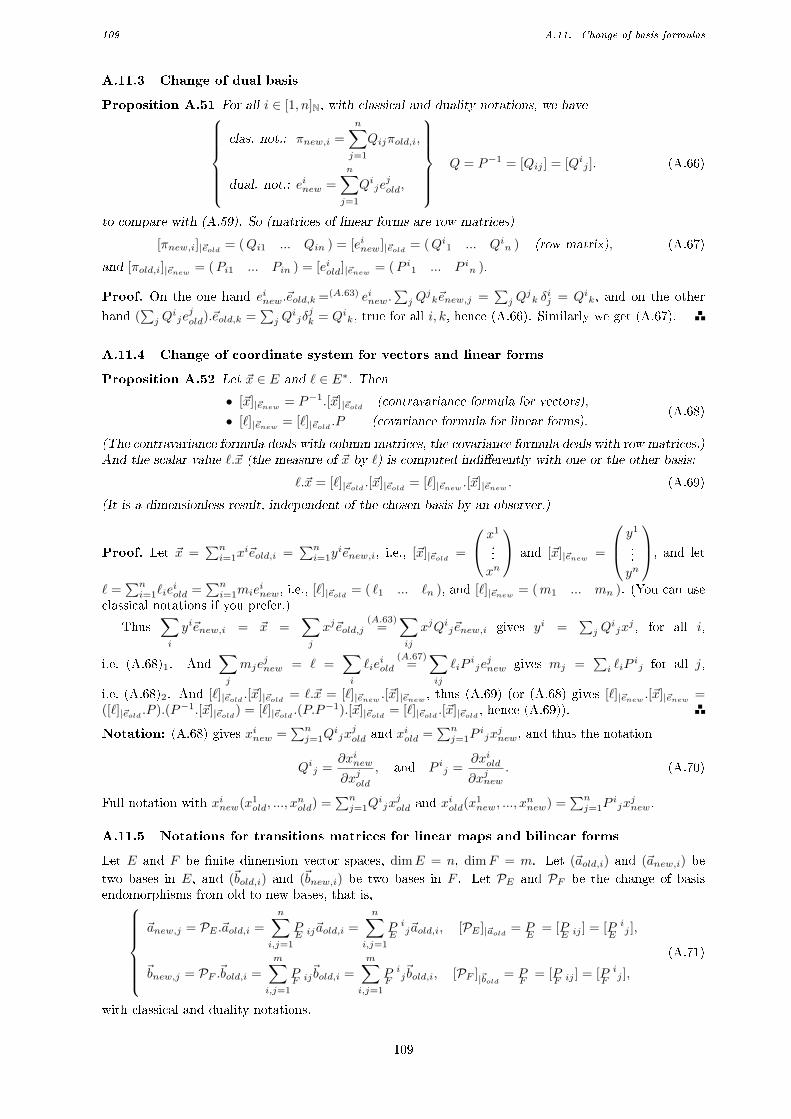
109 A.11. Change of basis formulas
A.11.3 Change of dual basis
Proposition A.51 For all i ∈ [1, n]N, with classical and duality notations, we haveclas. not.: πnew,i =
n∑j=1
Qijπold,i,
dual. not.: einew =
n∑j=1
Qijejold,
Q = P−1 = [Qij ] = [Qij ]. (A.66)
to compare with (A.59). So (matrices of linear forms are row matrices)
[πnew,i]|~eold = (Qi1 ... Qin ) = [einew]|~eold = (Qi1 ... Qin ) (row matrix), (A.67)
and [πold,i]|~enew = (Pi1 ... Pin ) = [eiold]|~enew = (P i1 ... P in ).
Proof. On the one hand einew.~eold,k =(A.63) einew.∑j Q
jk~enew,j =
∑j Q
jk δ
ij = Qik, and on the other
hand (∑j Q
ijejold).~eold,k =
∑j Q
ijδjk = Qik, true for all i, k, hence (A.66). Similarly we get (A.67).
A.11.4 Change of coordinate system for vectors and linear forms
Proposition A.52 Let ~x ∈ E and ` ∈ E∗. Then• [~x]|~enew = P−1.[~x]|~eold (contravariance formula for vectors),
• [`]|~enew = [`]|~eold .P (covariance formula for linear forms).(A.68)
(The contravariance formula deals with column matrices, the covariance formula deals with row matrices.)And the scalar value `.~x (the measure of ~x by `) is computed indierently with one or the other basis:
`.~x = [`]|~eold .[~x]|~eold = [`]|~enew .[~x]|~enew . (A.69)
(It is a dimensionless result, independent of the chosen basis by an observer.)
Proof. Let ~x =∑ni=1x
i~eold,i =∑ni=1y
i~enew,i, i.e., [~x]|~eold =
x1
...xn
and [~x]|~enew =
y1
...yn
, and let
` =∑ni=1`ie
iold =
∑ni=1mie
inew, i.e., [`]|~eold = ( `1 ... `n ), and [`]|~enew = (m1 ... mn ). (You can use
classical notations if you prefer.)
Thus∑i
yi~enew,i = ~x =∑j
xj~eold,j(A.63)
=∑ij
xjQij~enew,i gives yi =∑j Q
ijxj , for all i,
i.e. (A.68)1. And∑j
mjejnew = ` =
∑i
`ieiold
(A.67)=
∑ij
`iPijejnew gives mj =
∑i `iP
ij for all j,
i.e. (A.68)2. And [`]|~eold .[~x]|~eold = `.~x = [`]|~enew .[~x]|~enew , thus (A.69) (or (A.68) gives [`]|~enew .[~x]|~enew =([`]|~eold .P ).(P−1.[~x]|~eold) = [`]|~eold .(P.P
−1).[~x]|~eold = [`]|~eold .[~x]|~eold , hence (A.69)).
Notation: (A.68) gives xinew =∑nj=1Q
ijxjold and x
iold =
∑nj=1P
ijxjnew, and thus the notation
Qij =∂xinew
∂xjold, and P ij =
∂xiold∂xjnew
. (A.70)
Full notation with xinew(x1old, ..., x
nold) =
∑nj=1Q
ijxjold and x
iold(x
1new, ..., x
nnew) =
∑nj=1P
ijxjnew.
A.11.5 Notations for transitions matrices for linear maps and bilinear forms
Let E and F be nite dimension vector spaces, dimE = n, dimF = m. Let (~aold,i) and (~anew,i) be
two bases in E, and (~bold,i) and (~bnew,i) be two bases in F . Let PE and PF be the change of basisendomorphisms from old to new bases, that is,
~anew,j = PE .~aold,i =
n∑i,j=1
PE ij~aold,i =
n∑i,j=1
PE
ij~aold,i, [PE ]|~aold = P
E= [P
E ij ] = [PE
ij ],
~bnew,j = PF .~bold,i =
m∑i,j=1
PF ij
~bold,i =
m∑i,j=1
PF
ij~bold,i, [PF ]|~bold = P
F= [P
F ij ] = [PF
ij ],
(A.71)
with classical and duality notations.
109
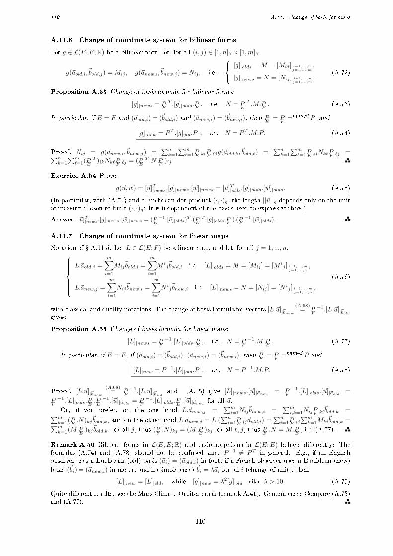
110 A.11. Change of basis formulas
A.11.6 Change of coordinate system for bilinear forms
Let g ∈ L(E,F ;R) be a bilinear form, let, for all (i, j) ∈ [1, n]N × [1,m]N,
g(~aold,i,~bold,j) = Mij , g(~anew,i,~bnew,j) = Nij , i.e.
[g]|olds = M = [Mij ] i=1,...,nj=1,...,m
,
[g]|news = N = [Nij ] i=1,...,nj=1,...,m
.(A.72)
Proposition A.53 Change of basis formula for bilinear forms:
[g]|news = PE
T .[g]|olds.PF , i.e. N = PE
T .M.PF. (A.73)
In particular, if E = F and (~aold,i) = (~bold,i) and (~anew,i) = (~bnew,i), then PE = PF
=named P , and
[g]|new = PT .[g]old.P , i.e. N = PT .M.P. (A.74)
Proof. Nij = g(~anew,i,~bnew,j) =∑nk=1
∑m`=1PE kiPF `jg(~aold,k,~bold,`) =
∑nk=1
∑m`=1PE kiNk`PF `j =∑n
k=1
∑m`=1(P
E
T )ikNk`PF `j = (PE
T .N.PF
)ij .
Exercice A.54 Prove:
g(~u, ~w) = [~u]T|news.[g]|news.[~w]|news = [~u]T|olds.[g]|olds.[~w]|olds. (A.75)
(In particular, with (A.74) and a Euclidean dot product (·, ·)g, the length ||~u||g depends only on the unitof measure chosen to built (·, ·)g: It is independent of the bases used to express vectors.)
Answer. [~u]T|news.[g]|news.[~w]|news = (PE−1.[~u]|olds)
T .(PET .[g]|olds.PF ).(P
F−1.[~w]|olds).
A.11.7 Change of coordinate system for linear maps
Notation of A.11.5. Let L ∈ L(E;F ) be a linear map, and let, for all j = 1, ..., n,L.~aold,j =
m∑i=1
Mij~bold,i =
m∑i=1
M ij~bold,i i.e. [L]|olds = M = [Mij ] = [M i
j ] i=1,...,mj=1,...,n
,
L.~anew,j =
m∑i=1
Nij~bnew,i =
m∑i=1
N ij~bnew,i i.e. [L]|news = N = [Nij ] = [N i
j ] i=1,...,mj=1,...,n
,
(A.76)
with classical and duality notations. The change of basis formula for vectors [L.~u]|~bnew(A.68)
= PF
−1.[L.~u]|~boldgives:
Proposition A.55 Change of bases formula for linear maps:
[L]|news = PF
−1.[L]|olds.PE , i.e. N = PF
−1.M.PE. (A.77)
In particular, if E = F , if (~aold,i) = (~bold,i), (~anew,i) = (~bnew,i), then PF = PF
=named P and
[L]|new = P−1.[L]|old.P , i.e. N = P−1.M.P. (A.78)
Proof. [L.~u]|~bnew(A.68)
= PF
−1.[L.~u]|~bold and (A.15) give [L]|news.[~u]|~anew = PF
−1.[L]|olds.[~u]|~aold =
PF
−1.[L]|olds.PE .PE−1.[~u]|~aold = P
F
−1.[L]|olds.PE .[~u]|~anew for all ~u.
Or, if you prefer, on the one hand L.~anew,j =∑mi=1Nij
~bnew,i =∑mi,k=1NijPF ki
~bold,k =∑mk=1(P
F.N)kj~bold,k, and on the other hand L.~anew,j = L.(
∑ni=1PE ij~aold,i) =
∑ni=1PE ij
∑mk=1Mki
~bold,k =∑mk=1(M.P
E)kj~bold,k, for all j, thus (P
F.N)kj = (M.P
E)kj for all k, j, thus PF .N = M.P
E, i.e. (A.77).
Remark A.56 Bilinear forms in L(E,E;R) and endomorphisms in L(E;E) behave dierently: Theformulas (A.74) and (A.78) should not be confused since P−1 6= PT in general. E.g., if an Englishobserver uses a Euclidean (old) basis (~ai) = (~aold,i) in foot, if a French observer uses a Euclidean (new)
basis (~bi) = (~anew,i) in meter, and if (simple case) ~bi = λ~ai for all i (change of unit), then
[L]|new = [L]|old, while [g]|new = λ2[g]|old with λ > 10. (A.79)
Quite dierent results, see the Mars Climate Orbiter crash (remark A.41). General case: Compare (A.73)and (A.77).
110
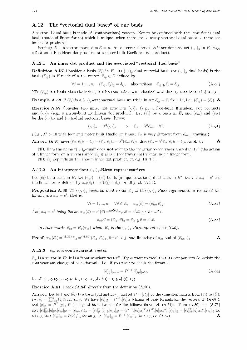
111 A.12. The vectorial dual bases of one basis
A.12 The vectorial dual bases of one basis
A vectorial dual basis is made of (contravariant) vectors. Not to be confused with the (covariant) dualbasis (made of linear forms) which is unique, when there are as many vectorial dual bases as there areinner dot products.
Setting: E is a vector space, dimE = n. An observer chooses an inner dot product (·, ·)g in E (e.g.,a foot-built Euclidean dot product, or a meter-built Euclidean dot product).
A.12.1 An inner dot product and the associated vectorial dual basis
Denition A.57 Consider a basis (~ei) in E. Its (·, ·)g-dual vectorial basis (or (·, ·)g-dual basis) is thebasis (~eig) in E made of n the vectors ~eig ∈ E dened by
∀j = 1, ..., n, (~eig, ~ej)g = δij , also written ~eig •g ~ei = δij . (A.80)
NB: (~eig) is a basis, thus the index i is a bottom index, with classical and duality notations, cf. A.10.1.
Example A.58 If (~ei) is a (·, ·)g-orthonormal basis we trivially get ~eig = ~ei for all i, i.e., (~eig) = (~ei).
Exercice A.59 Consider two inner dot products (·, ·)a (e.g., a foot-built Euclidean dot product)and (·, ·)b (e.g., a meter-built Euclidean dot product). Let (~ei) be a basis in E, and (~eia) and (~eib)be the (·, ·)a- and (·, ·)b-dual vectorial bases. Prove:
(·, ·)a = λ2(·, ·)b =⇒ ~eib = λ2~eia, ∀i. (A.81)
(E.g., λ2 > 10 with foot and meter built Euclidean bases: ~eib is very dierent from ~eia. Drawing.)
Answer. (A.80) gives (~eib, ~ej)b = δij = (~eia, ~ej)a = λ2(~eia, ~ej)b, thus (~eib − λ2~eia, ~ej)b = δij , for all i, j.
NB: Here the name (·, ·)g-dual does not refer to the covariance-contravariance duality (the actionof a linear form on a vector) since ~eig ∈ E is a (contravariant) vector, not a linear form.
NB: ~eig depends on the chosen inner dot product, cf. e.g. (A.81).
A.12.2 An interpretation: (·, ·)g-Riesz representatives
Let (~ei) be a basis in E; Let (πei) = (ei) be its (unique covariant) dual basis in E∗, i.e. the πei = ei arethe linear forms dened by πei(~ej) = ei(~ej) = δij for all j, cf. (A.33).
Proposition A.60 The (·, ·)g-vectorial dual vector ~eig is the (·, ·)g-Riesz representation vector of thelinear form πei = ei, that is,
∀i = 1, ..., n, ∀~v ∈ E, πei(~v) = (~eig, ~v)g. (A.82)
And πei = ei being linear, πei(~v) = ei(~v) =noted πei.~v = ei.~v, so, for all i,
πei.~v = (~eig, ~v)g = ~eig •g ~v = ei.~v. (A.83)
In other words, ~eig = Rg(πei) where Rg is the (·, ·)g-Riesz operator, see (C.6).
Proof. πei(~ej) =(A.33) δij =(A.80)(~eig, ~ej)g, for all i, j, and linearity of πei and of (~eig, ·)g.
A.12.3 ~eig is a contravariant vector
~eig is a vector in E: It is a contravariant vector. If you want to see that its components do satisfy thecontravariant change of basis formula, i.e., if you want to check the formula
[~ejg]|new = P−1.[~ejg]|old, (A.84)
for all j, go to exercise A.61, or apply C.1.6 and (C.18).
Exercice A.61 Check (A.84) directly from the denition (A.80).
Answer. Let (~ai) and (~bi) two bases (old and new), and let P = [Pij ] be the transition matrix from (~ai) to (~bi),
i.e., ~bj =∑ni=1Pij~ai for all j. We have [~ej ]|~b = P−1.[~ej ]|~a (change of basis formula for the vectors, cf. (A.68)),
and [g]|~b = PT .[g]|~a.P (change of basis formula for the bilinear forms, cf. (A.74)). Then (A.80) and (A.75)
give [~ei]T|~a.[g]|~a.[~ejg]|~a = (~ejg, ~ei)g = [~ei]
T|~b.[g]|~b.[~ejg]|~b = (P−1.[~ei]|~a)T .(PT .[g]|~a.P ).[~ejg]|~b = [~ej ]
T|~a.[g]|~a.P.[~eig]|~b for
all i, j, thus [~ejg]|~a = P.[~ejg]|~b for all j, i.e. [~ejg]|~b = P−1.[~ejg]|~a for all j, i.e. (A.84).
111
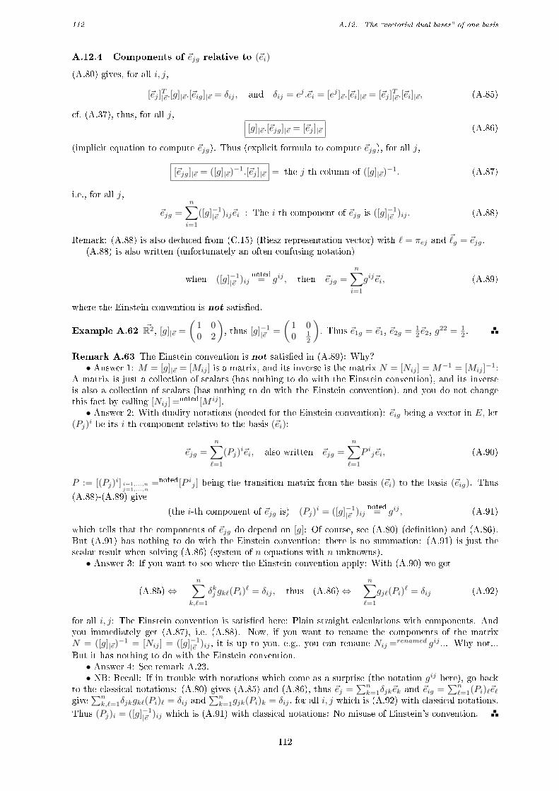
112 A.12. The vectorial dual bases of one basis
A.12.4 Components of ~ejg relative to (~ei)
(A.80) gives, for all i, j,
[~ej ]T|~e.[g]|~e.[~eig]|~e = δij , and δij = ej .~ei = [ej ]~e.[~ei]|~e = [~ej ]
T|~e.[~ei]|~e, (A.85)
cf. (A.37), thus, for all j,
[g]|~e.[~ejg]|~e = [~ej ]|~e (A.86)
(implicit equation to compute ~ejg). Thus (explicit formula to compute ~ejg), for all j,
[~ejg]|~e = ([g]|~e)−1.[~ej ]|~e = the j-th column of ([g]|~e)
−1. (A.87)
i.e., for all j,
~ejg =
n∑i=1
([g]−1|~e )ij~ei : The i-th component of ~ejg is ([g]−1
|~e )ij . (A.88)
Remark: (A.88) is also deduced from (C.15) (Riesz representation vector) with ` = πej and ~g = ~ejg.(A.88) is also written (unfortunately an often confusing notation)
when ([g]−1|~e )ij
noted= gij , then ~ejg =
n∑i=1
gij~ei, (A.89)
where the Einstein convention is not satised.
Example A.62 ~R2, [g]|~e =
(1 00 2
), thus [g]−1
|~e =
(1 00 1
2
). Thus ~e1g = ~e1, ~e2g = 1
2~e2, g22 = 1
2 .
Remark A.63 The Einstein convention is not satised in (A.89): Why?• Answer 1: M = [g]|~e = [Mij ] is a matrix, and its inverse is the matrix N = [Nij ] = M−1 = [Mij ]
−1:A matrix is just a collection of scalars (has nothing to do with the Einstein convention), and its inverseis also a collection of scalars (has nothing to do with the Einstein convention), and you do not changethis fact by calling [Nij ] =noted[M ij ].• Answer 2: With duality notations (needed for the Einstein convention): ~eig being a vector in E, let
(Pj)i be its i-th component relative to the basis (~ei):
~ejg =
n∑`=1
(Pj)i~ei, also written ~ejg =
n∑`=1
P ij~ei, (A.90)
P := [(Pj)i] i=1,...,nj=1,...,n
=noted[P ij ] being the transition matrix from the basis (~ei) to the basis (~eig). Thus
(A.88)-(A.89) give
(the i-th component of ~ejg is) (Pj)i = ([g]−1
|~e )ijnoted
= gij , (A.91)
which tells that the components of ~ejg do depend on [g]: Of course, see (A.80) (denition) and (A.86).But (A.91) has nothing to do with the Einstein convention: there is no summation: (A.91) is just thescalar result when solving (A.86) (system of n equations with n unknowns).• Answer 3: If you want to see where the Einstein convention apply: With (A.90) we get
(A.85)⇔n∑
k,`=1
δkj gk`(Pi)` = δij , thus (A.86)⇔
n∑`=1
gj`(Pi)` = δij (A.92)
for all i, j: The Einstein convention is satised here: Plain straight calculations with components. Andyou immediately get (A.87), i.e. (A.88). Now, if you want to rename the components of the matrixN = ([g]|~e)
−1 = [Nij ] = ([g]−1|~e )ij , it is up to you, e.g., you can rename Nij =renamed gij ... Why not...
But it has nothing to do with the Einstein convention.• Answer 4: See remark A.23.• NB: Recall: If in trouble with notations which come as a surprise (the notation gij here), go back
to the classical notations: (A.80) gives (A.85) and (A.86), thus ~ej =∑nk=1δjk~ek and ~eig =
∑n`=1(Pi)`~e`
give∑nk,`=1δjkgk`(Pi)` = δij and
∑nk=1gjk(Pi)k = δij , for all i, j which is (A.92) with classical notations.
Thus (Pj)i = ([g]−1|~e )ij which is (A.91) with classical notations: No misuse of Einstein's convention.
112
113 A.12. The vectorial dual bases of one basis
Remark A.64 We have just seen multiple notations for the components of ~ejg relative to the basis (~ei):
~ejg =
n∑j=1
(Pj)i~ei =
n∑j=1
Pij~ei︸ ︷︷ ︸clas.
=
n∑j=1
(Pj)i~ei =
n∑j=1
P ij~ei︸ ︷︷ ︸dual
= P.~ei, (A.93)
where P ∈ L(~Rn; ~Rn) is the change of basis endomorphism from (~ei) to (~eig), which matrix [P]|~e = [Pij ]
is also written [(Pj)i] = [Pj)i] = [P ij ]: Thus [~ejg]|~e =
P1j
...Pnj
=
(Pj)1
...(Pj)n
=
P 1j
...Pnj
=
(Pj)1
...(Pj)
n
=
[P]|~e.[~ej ]|~e. You can choose any notation, depending on your current mood: Pij = (Pj)i = P ij = (Pj)i.
A.12.5 Notation problem
Notation problem with duality notations: Because the components (Pj)i of ~ejg are equal to
([g]−1|~e )ij =noted gij , cf. (A.88)-(A.89), some authors rename ~ejg as ~e
j ... to get ~ej =∑ni=1g
ij~ei...
But doing so they despise Einstein's convention:• It is up to you to rename ~ejg to ~ej , but it has nothing to do with Einstein's convention which is
meant to respect covariance and contravariance. If you do want to see the Einstein convention, see (A.92).•We insist: The contravariant vectors ~ejg make a basis (~ejg) in E, cf. (A.84): Named with low indices,
cf. A.10.1. And renaming ~ejg to ~ej has nothing to do with the the covariancecontravariance dualitynotation (Einstein's convention). This renaming just adds confusion to the confusion.• With classical notations, there is no possible confusion regarding covariance or contravariance: If
you know from the start that ~ejg =∑ni=1Pij~ei is contravariant, then it is!
Recall: If you have the slightest doubt about duality notations (or with notations that appear as asurprise), go back to classical notations: Here ~ejg =
∑ni=1Pij~ei =
∑ni=1([g]−1
|~e )ij~ei ∈ E (a contravariant
vector), and no possible misinterpretation.
A.12.6 (Huge) dierences between the (covariant) dual basis and a dual vectorial basis
1. A basis (~ei) has an innite number of vectorial dual bases (~eig), as many as the number of innerdot products (·, ·)g (as many as observers), see (A.87).
2. While a basis (~ei) has a unique dual basis (πei)dual= (ei), intrinsic to the basis (~ei), cf. (A.33). In
particular two observers who consider the same basis (~ei) do have the same dual basis (πei) = (ei)even if they use dierent Euclidean dot products.
3. πei = ei is covariant, while ~ei and ~eig are contravariant. We insist: (~eig) is linked to (~ei) byan endomorphism P ∈ L(E;E) and its transition matrix [P ij ], cf. (A.93). When there can't beany transition matrix between (~ei) and (πei) = (ei): The vector ~ei ∈ E and the (linear) functionπei = ei ∈ E∗ don't live in the same vector space.
4. If you y, it is vital to use the dual basis (πei) = (ei): It is possibly fatal if you confuse foot and meterat takeo (through the choice of a Euclidean dot product (·, ·)g or (·, ·)h), and at landing (if yousurvived takeo). See e.g. the Mars Climate Orbiter crash, remark A.41. Einstein's convention canhelp... only if it is really followed...
5. The push-forward of a vector eld ~v, cf. (10.28), is dierent from the push-forward of a one-form α,cf. (13.3). Thus vectors and linear forms (contravariance and covariance) should not be confused.
6. The Lie derivative of a vector eld ~v, cf. (15.17), is dierent from the Lie derivative of a one-form α,cf. (15.49). Thus vectors and linear forms (contravariance and covariance) should not be confused.
A.12.7 About the notation gij
The notation [gij ] := [gij ]−1 = [g]−1
|~e of the inverse of the matrix [gij ], cf. (A.88), is due to the denition
of the Riesz associated inner dot product g] in L(E∗, E∗;R): It is dened by, for all `,m ∈ E∗,
g](`,m) := g(~g, ~mg) when ∀~w ∈ E, `.~w = (~g, ~w)g and m.~w = (~mg, ~w)g, (A.94)
113
114 A.13. The adjoint of a linear map
the (·, ·)g-Riesz representation having been applied twice, cf. (C.2). In particular, relative to a basis (~ei)in E and with its dual basis (ei) (duality notations),
(g])ij := g](ei, ej)(A.94)
= g(~eig, ~ejg) = ([g]|~eg )ij
= [~eig]T|~e.[g]|~e.[~ejg]|~e = ([~ei]
T|~e.[g]−1
|~e ).[g]|~e.([g]−1|~e .[~ej ]|~e)
= [~ei]T|~e.[g]−1
|~e .[~ej ]|~e = ([g]−1|~e )ij ,
(A.95)
thus[g]]|~e = [g]−1
|~e (= [g]|~eg ). (A.96)
With the classical notations:
(g])ij := g](πei, πej) = [πei]|πe .[g]]|πe .[πej ]
T|πe
= g(~eig, ~ejg) = [~ei]T|~e.[g]−1
|~e .[~ej ]|~e (= ([g]−1|~e )ij).
(A.97)
(NB: g] is rarely useful in continuum mechanics.)
Exercice A.65 How do we compute g](`,m) with matrix computations?
Answer. With a basis (ei) in E∗, ` =∑ni=1`ie
i and m =∑nj=1mje
j , we get g](`,m) =∑ni,j=1`imjg
](ei, ej) =∑ni,j=1`ig
ijmj . A linear form being represented by a row matrix, we get g](`,m) = [`]|~e.[g]]|~e.[m]T|~e.
Exercice A.66 What is the(
11
)tensor that you create from the
(02
)tensor (·, ·)g when using the (·, ·)g-
Riesz representation theorem just once? (We have just seen that the(
20
)tensor g] was created from the(
02
)tensor (·, ·)g using twice the (·, ·)g-Riesz representation theorem.) Why is the reverse question trivial?
Answer. Let g\ ∈ L(E∗, E;R) be dened by g\(`, ~w) = (~g, ~w)g where ~g is the (·, ·)g-Riesz representation
vector of `, that is, ~g is dened by `.~u = (~g, ~u)g for all ~u ∈ E. We immediately get g\(`, ~w) = `. ~w for all(`, ~w) ∈ E∗ × E: So, g\ is naturally canonically represented by the identity I ∈ L(E;E): For all (`, ~w) ∈ E∗ × Ewe have g\(`, ~w) = `.I. ~w = `. ~w: Thus g\ (bilinear form) is naturally associated with the identity (endomorphism).
The reverse is trivial: 1- Start from I ∈ L(E;E) the identity operator (observer independent); 2- Then
identied I with the(
11
)tensor I ∈ L(E∗, E;R) dened by I(`, ~w) = `. ~w; 3- Then (·, ·)g-associate I with the
(02
)tensor I[ created when using the (·, ·)g-Riesz representation theorem just once, that is, I[(~g, ~w) = I(`, ~w) when~g is the (·, ·)g-Riesz representation vector of `: you get I[ = g.
(So, I = g\ and I[ = g and I] = g] for Riesz representations with (·, ·)g.)
A.13 The adjoint of a linear map
(Dierence with the transposed: If L is a linear map, then L as only one adjoint linear map L∗, whileL has many transposed LTgh since a transposed depends on inner dot products (·, ·)g and (·, ·)h.)
Here no inner dot product is introduced. And, as usual, we rst give the denition (qualitativeapproach), and second, the quantication with bases and components.
Let E and F be two nite dimension vector spaces.
Denition A.67 If L ∈ L(E;F ), then its adjoint is the linear map L∗ ∈ L(F ∗;E∗) canonically denedby
L∗ :
F ∗ → E∗
m → L∗(m) := m L,(A.98)
i.e.,(L∗(m))(~u) := m(L(~u)), ∀(~u,m) ∈ E × F ∗. (A.99)
And the linearity of L and L∗ makes it possible to use the dot notation (linearity notation)
L∗.m := m.L, and (L∗.m).~u := m.L.~u. (A.100)
(The dual L∗ cannot be confused with the transposed which requires inner dot products, cf. (A.24).)
114
115 B.1. Euclidean basis
Quantication: Let (~ai) be a basis in E, (~bi) be a basis in F , and (πai) and (πbi) be the dual bases.Let
[L]|~a,~b = [Lij ] i=1,...,mj=1,...,n
, and [L∗]|b,a = [(L∗)ij ] i=1,...,nj=1,...,m
, (A.101)
that is,
L.~aj =
m∑i=1
Lij~bi, and L∗.πbj =
n∑i=1
(L∗)ijπai. (A.102)
Then (A.100) gives (L∗.πbj).~ai = πbj .(L.~ai), that is,
(L∗)ij = Lji, i.e. [L∗]|b,a = [(L]|~a,~b)T (transposed matrix). (A.103)
To compare with (A.25) (there is no inner dot product here).(Duality notations: L∗.bj =
∑ni=1(L∗)i
jai, and (L∗)ij = Lji.)
B Euclidean Frameworks
Time and space are decoupled (classical mechanics). Rn is the geometric ane space, n = 1, 2, 3, and~Rn is the associated vector space (made of bi-point vectors) which will be equipped with measuringinstruments: Euclidean dot products to get angles and lengths.
B.1 Euclidean basis
Manufacturing of a Euclidean basis.An observer chooses a unit of measure (foot, meter, a unit of length used by Euclid, the diameter a
of pipe...) and makes a unit rod of length 1 in this unit. Postulate: The length of the rod does notdepend on its direction in space.
• Space dimension n = 1: This rod models a vector ~e1 which makes a basis (~e1) called the Euclideanbasis relative to the chosen unit of measure.
• Space dimension n ≥ 2:- The observers makes three rods of length 3, 4 and 5, and makes a triangle (A,B,C), where A, B
and C are the vertices, and A not on the side on length 5.- Since 32 + 42 = 52, the triangle (A,B,C) is said to have a right angle at A (Pythagoras).
- Two vectors ~u and ~w in Rn are orthogonal i the triangle (A,B,C) can be positioned such that ~AB
and ~AC are parallel to ~u and ~w.- A basis (~ei)i=1,...,n is Euclidean relative to the chosen unit of measurement i the ~ei are two to two
orthogonal and their length is 1 (relative to the chosen unit).
Example B.1 An English observer denes a Euclidean basis (~ai) using the foot. A French observer
denes a Euclidean basis (~bi) using the meter. We have
1 foot = µmeter, µ = 0.3048, and 1 meter = λ foot, λ =1
µ' 3.28. (B.1)
(µ = 0, 3048 is the ocial length in meter for the English foot.) E.g., the bases are aligned i, for all i,
~bi = λ~ai (change of measurement unit), (B.2)
and the transition matrix from (~ai) to (~bi) is then P = λI, thus PT = P , PT .P = λ2I and P−1 = 1λI.
Remark B.2 The bases used in practice are not all Euclidean. See example A.40, especially if you y.
B.2 Euclidean dot product
Denition B.3 Consider an observer who has built (or chosen) his Euclidean basis (~ei), cf. B.1. The
associated Euclidean dot product is the bilinear form g(·, ·) = (·, ·)g ∈ L(~Rn, ~Rn;R) dened by
g(~ei, ~ej) = δij = gij , ∀i, j, i.e. [g]|~e = [δij ] = I, (B.3)
cf. prop. A.11.
115
116 B.3. Change of Euclidean basis
That is, with tensorial and duality notations, cf. (A.49), (πei) = (ei) being the dual basis of (~ei) (withclassical and duality notations),
(·, ·)gclas.=
n∑i=1
πei ⊗ πeidual=
n∑i=1
ei ⊗ ei. (B.4)
(If you want to use the Einstein convention: (·, ·)g :=∑ni,j=1δije
i ⊗ ej , cf. (B.3).) So, for all ~x, ~y ∈ ~Rn,with ~x =
∑ni=1xi~ei =
∑ni=1x
i~ei and ~y =∑ni=1yi~ei =
∑ni=1y
i~ei,
(~x, ~y)gclas.=
n∑i=1
xiyidual=
n∑i=1
xiyi = [~x]T|~e.[~y]|~e. (B.5)
(If you want to use the Einstein convention: (~x, ~y)g :=∑ni,j=1δijx
iyj = [~x]T|~e.[g]|~e.[~y]|~e.)
Denition B.4 The associated norm is ||.||g :=√
(·, ·)g, and the length of a vector ~x relative to the
chosen Euclidean unit of measurement is ||~x||g :=√
(~x, ~x)g.
Thus with the Euclidean basis (~ei) (used to build (·, ·)g), if ~x =∑ni=1xi~ei =
∑ni=1x
i~ei, then ||~x||g =√∑ni=1x
2i =
√∑ni=1(xi)2 is the length of ~x relative to the chosen Euclidean unit of measure (Pythagoras).
(If you want to use the Einstein convention:: ||~x||g :=√∑n
i,j=1δijxixj .)
Denition B.5 Two vectors ~x, ~y are (·, ·)g-orthogonal i (~x, ~y)g = 0.
Denition B.6 The angle θ(~x, ~y) between two vectors ~x, ~y ∈ ~Rn − ~0 is dened by
cos(θ(~x, ~y)) = (~x
||~x||g,
~y
||~y||g)g (= cos(θ(~y, ~x))). (B.6)
(With a calculator, this formula gives θ(~x, ~y) = arccos(( ~x||~x||g ,
~y||~y||g )g) a value in [0, π].)
Denition B.7 A basis (~bi) such that (~bi,~bj)g = δij , for all i, j = 1, ..., n, is called a (·, ·)g-orthonormalbasis.
Proposition B.8 If (~ai) and (~bi) are two (·, ·)g-orthonormal bases, and if P is the transition matrix
from (~ai) to (~bi), then PT .P = I, and we have (·, ·)g =
∑ni=1a
i ⊗ ai =∑ni=1b
i ⊗ bi.
Proof. ~bj =∑ni=1P
ij~ai gives δij = (~bi,~bj)g =
∑nk,`=1P
ki P
`j (~ak,~a`)g =
∑nk,`=1P
ki P
`j δk` =
∑nk=1P
ki P
kj =∑n
k=1(PT )ikPkj = (PT .P )ij for all i, j, thus P
T .P = [(PT .P )ij ] = [δij ] = I.
And for the dual bases we have ai =∑nj=1P
ij bj , cf. (A.67). Thus
∑ni=1a
i⊗ai =∑ni,k,`=1P
ikP
i` bk⊗b` =∑n
k,`=1δk`bk ⊗ b` =
∑nk=1b
k ⊗ bk, that is, [g]|~a = [g]|~b = I.
B.3 Change of Euclidean basis
Let (~ai) (e.g. built with the foot) and (~bi) (e.g. built with the meter) be two Euclidean bases in ~Rn. Let(·, ·)g and (·, ·)h be the associated Euclidean dot products in ~Rn.
B.3.1 Two Euclidean dot products are proportional
Proposition B.9 If λ = ||~b1||g, then ||~bi||g = λ for all i = 1, ..., n (change of unit). The Euclidean dotproducts (·, ·)g and (·, ·)h are necessarily proportional:
if λ = ||~b1||g then (·, ·)g = λ2(·, ·)h and ||.||g = λ||.||h. (B.7)
(Useful if e.g. you want to use results of Newton, Descartes... or work with another observer.)
Proof. By denition of a Euclidean basis, the length of the rod that enabled to dene (~bi) is independent
of i, cf. the postulate B.1, thus ||~bi||g = ||~b1||g for all i.Thus (~bi,~bi)g = ||~bi||2g = λ2 = λ2(~bi,~bi)h for all i, since (~bi,~bi)h = ||~bi||2h = 1. And if i 6= j then
two Euclidean basis vectors form a right angle (Pythagoras), thus (~bi,~bj)g = 0 = (~bi,~bj)h when i 6= j,
cf. (B.4). Hence (~bi,~bj)g = λ2(~bi,~bj)h for all i, j, thus (B.7).
116
117 B.4. Euclidean transposed of the deformation gradient
Example B.10 Continuation of example B.1. (·, ·)a =∑ni=1a
i⊗ai is the English Euclidean dot product(foot), and (·, ·)b =
∑ni=1b
i ⊗ bi is the French Euclidean dot product (meter). (B.7) and (B.1) give:
(·, ·)a = λ2(·, ·)b and ||.||a = λ||.||b, with λ ' 3.28 and λ2 ' 10.76. (B.8)
E.g., if ~w is s.t. ||~w||b = 1 (its length is 1 meter), then ||~w||a = λ (its length is λ ' 3.28 foot).
B.3.2 Counterexample : non existence of a Euclidean dot product
1- Thermodynamic: Let T be the temperature and V the volume, and consider the Cartesian vector
space ~R2 = (T, V ) = R × R. There is no associated Euclidean dot product: An associated normwould give ||(T, V )|| =
√T 2 + V 2 ∈ R which is meaningless (you don't add Kelvin and cubic meters,
even squared...). See A.8.5.
2- Polar coordinate system, see example 10.17: A parametric vector ~q = (r, θ) ∈ R × R has no normthat is physically meaningful:
√r2 + θ2 has no physical meaning.
B.4 Euclidean transposed of the deformation gradient
Let n ∈ 1, 2, 3 and consider a linear map L ∈ L(~Rnt0 ; ~Rnt ) (e.g., L = F t0t (P )).
Let (·, ·)G be an inner dot product in ~Rnt0 (used in the past by someone), and let (·, ·)a and (·, ·)bbe inner dot products in ~Rnt (the actual space where the results are observed by two observers, e.g.,English (·, ·)a and French (·, ·)b). Let LTGa and LTGb be the transposed of L relative to the dot products,
that is, LTGa and LTGb in L(~Rnt ; ~Rnt0) are characterized by
(LTGa.~y, ~X)G = (L. ~X, ~y)a and (LTGb.~y, ~X)G = (L. ~X, ~y)b, (B.9)
for all ~X ∈ ~Rnt0 and all ~y ∈ ~Rnt , cf. (A.24).
Proposition B.11 If (·, ·)a and (·, ·)b are Euclidean dot products, then
(·, ·)a = λ2(·, ·)b =⇒ LTGa = λ2LTGb ∈ L(~Rnt ; ~Rnt0) (B.10)
(a vector type relation, as in (5.34) or (C.10)). NB: Do not forget λ2 if an French observer works with aEnglish observer at t (or NASA with Boeing, cf. remark A.41).
Proof. (LTGa.~y, ~X)G(B.9)
= (L. ~X, ~y)a(B.7)
= λ2(L. ~X, ~y)b(B.9)
= λ2(LTGb.~y,~X)G for all ~X ∈ ~Rnt0 and all ~y ∈ ~Rnt ,
thus LTGa.~y = λ2LTGb.~y for all ~y ∈ ~Rnt .
B.5 The Euclidean transposed for endomorphisms
Let n ∈ 1, 2, 3 and consider an endomorphism L ∈ L(~Rn; ~Rn) (e.g. L = d~vt(p) ∈ L(~Rnt ; ~Rnt ) the
dierential of the Eulerian velocity). Let (·, ·)a and (·, ·)b be dot products in ~Rn. Let LTa and LTb be the
transposed of L relative to (·, ·)a and (·, ·)b, that is, LTa and LTb in L(~Rn; ~Rn) are the endomorphisms
dened by, for all ~x, ~y ∈ ~Rn, cf. (A.17),
(LTa .~y, ~x)a = (L.~x, ~y)a, and (LTb .~y, ~x)b = (L.~x, ~y)b. (B.11)
Proposition B.12 If (·, ·)a and (·, ·)b are Euclidean dot products, then
(Euclidean dot products) LTa = LTbnoted
= LT ∈ L(~Rnt ; ~Rnt ) (B.12)
(an endomorphism type relation): Thus we can speak of the Euclidean transposed of an endomorphism.
Proof. (LTa .~y, ~x)a(B.11)
= (L.~x, ~y)a(B.7)
= λ2(L.~x, ~y)b(B.11)
= λ2(LTb .~y, ~x)b(B.7)
= (LTb .~y, ~x)a for all ~x, ~y ∈ ~Rn, thusLTa .~y = LTb .~y for all ~y ∈ ~Rn.
117

118 C.1. The Riesz representation theorem
C Riesz representation theorem
C.1 The Riesz representation theorem
The goal is, when we have an inner dot product (·, ·)g, to represent a linear function by a vector thanksto (·, ·)g. It is in no way an identication: It is only a representation, or an association, allowed by achoice of a measuring tool (·, ·)g (observer dependent). In particular two observers with two dierentmeasuring tools get two dierent representation vectors (two dierent associations).
C.1.1 Framework
Framework: A Hilbert space (E, (·, ·)g), that is, a vector space E equipped with an inner dot product (·, ·)gand ||.||g the associated norm such that (E, ||.||g) is a complete space (a Banach space). And
E∗ = L(E;R) = the space of the linear and continuous forms E → R. (C.1)
NB:1- If E is nite dimensional: All norms are equivalent, (E, (·, ·)g) is a Hilbert space, and any linear
form is continuous. This is the usual framework in continuum mechanics with E = ~R3.2- If E is innite dimensional: Then two norms can be non equivalent, (E, ||.||g) can be non complete,
a linear form can be non continuous; And the Riesz representation theorem can only be applied tocontinuous linear forms. This is the usual framework in continuum mechanics with E = L2(Ω) the spaceof nite energy functions in Ω, thus it is the framework of the nite element method.
C.1.2 Riesz representation theorem
We have the easy statement, (·, ·)g being some inner dot product in E:
If ~v ∈ E (vector) then ∃!vg ∈ E∗ (linear continuous form) s.t. vg(~x) = (~v, ~x)g, ∀~x ∈ E. (C.2)
Moreover ||vg||E∗ = ||~v||g.Proof: Dene vg ∈ E∗ by vg(~x) = (~v, ~x)g for all ~x ∈ E, then use the CauchySchwarz inequality to
get |vg(~x)| = ||~v||g ||~x||g for all ~x ∈ E, thus ||vg||E∗ ≤ ||~v||g, and with ~x = ~v we get |vg(~v)| = ||~v||g ||~x||g,thus ||vg||E∗ ≥ ||~v||g. Thus ||vg||E∗ = ||~v||g <∞, thus vg is continuous.
The Riesz representation theorem concerns the converse:
Theorem C.1 (Riesz representation theorem, and denition) Let (E, (·, ·)g) be a Hilbert space,and E∗ be the space of linear continuous form on E.
If ` ∈ E∗ (linear continuous form) then ∃!~g ∈ E (vector) s.t. `(~x) = (~g, ~x)g, ∀~x ∈ E. (C.3)
Moreover ||~g||g = ||`||E∗ . The vector ~g = ~(g) ∈ E (which depends on g) is called the (·, ·)g-Rieszrepresentation vector of `.
Proof. If ` = 0 then ~g = ~0 (trivial). Suppose ` 6= 0. Let Ker` = `−1(0) (the kernel).If dimE = 1, it is trivial (exercise). Suppose dimE ≥ 2. Then Ker` 6= ~0. Since ` is continuous,
Ker` = `−1(0) is closed in the Hilbert space (E, (·, ·)g). Thus, if ~x ∈ E, then its (·, ·)g-projection~x0 ∈ Ker` on Ker` exists, is unique, and is given by:
∀~y0 ∈ Ker`, (~x− ~x0, ~y0)g = 0. (C.4)
In particular, if ~x /∈ Ker` (possible since ` 6= 0), let ~n = ~x−~x0
||~x−~x0||g ; So ~n is a unitary (·, ·)g-normal vector
to Ker` and (Ker`)⊥ = Vect~n since, ` being a linear form, codim(Ker`) = 1 and dim(Ker`)⊥ = 1. AndE = Ker`⊕(Ker`)⊥ since both vector spaces are closed. Thus if ~x ∈ E then ~x = ~x0+λ~n ∈ Ker`×(Ker`)⊥,where ~x0 ∈ Ker` and λ ∈ R; Thus (~x, ~n)g = λ and `(~x) = λ`(~n); Thus `(~x) = (~x, ~n)g`(~n) = (~x, `(~n)~n)g(bilinearity of (·, ·)g); Thus ~g := `(~n)~n satises (C.3). And if vectors ~g1 and ~
g2 satisfy (C.3) then
(~g1− ~g2, ~x)g = 0 for all ~x ∈ E, thus ~g1− ~g2 = 0. Thus ~g is unique. And the CauchySchwarz theorem
give ||`||E∗ = sup||~x||g=1 |`(~x)| = sup||~x||g=1 |(~g, ~x)g| = ||~g||g.
118
119 C.1. The Riesz representation theorem
C.1.3 Riesz representation mapping
Let SIDP (E) be the space of inner dot products in E. Then (C.3) gives the Riesz representation mapping:
R :
SIDP × E∗ → E
(g, `) → R(g, `) := ~g.
(C.5)
In particular, for a g ∈ SIDP (E) (that is, for the observer who has chosen g),
Rg = R(g, ·) :
(E∗, ||.||E∗) → (E, ||.||E)
` → Rg(`) = R(g, ·)(`) := R(g, `) (= ~g)
(C.6)
is an isomorphism (linear, bijective and ||`||E∗ = ||~g||E). And, for any ` ∈ E∗,
R(·, `) :
SIDP → E
g → R(·, `)(g) := R(g, `) (= ~g)
(C.7)
associates an observer (the one who chooses (·, ·)g) with ~(g) = ~g.
Remark C.2 You cannot identify a linear form ` with one of its Riesz representation vector: Whichone? ~g = R(g, `)? ~h = R(h, `)? (See e.g. (C.11).)
Notation. A ` ∈ E∗ being linear `(~x) =noted `.~x: The dot between ` and x is the usual duality dot(covariance-contravariance dot = linear form acting on a vector); It is not the dot of a inner dot product.If you want to use a dot notation for the inner dot product (·, ·)g, then (C.3) should be at least written
`.~x = ~g •g ~x, where ~
g •g ~x := (~g, ~x)g. (C.8)
At least, use a big dot notation like `.~x = ~ • ~x.
C.1.4 Change of Riesz representation vector: Euclidean case
For one linear form `, two observers with two Euclidean dot products (·, ·)a and (·, ·)b (e.g., one in foot
and one in meter) get two Riesz representation vectors ~a and ~b given by, cf. (C.3),
∀~x ∈ E, `.~x = (~a, ~x)a = (~b, ~x)b. (C.9)
Proposition C.3 Change of Euclidean Riesz representation vector:
If ∃λ > 0, (·, ·)a = λ2(·, ·)b then ~b = λ2~
a. (C.10)
Conversely, if ~b = λ2~a for all linear forms `, then (·, ·)a = λ2(·, ·)b.
NB: (C.10) is a change of vector formula (one linear form, two vectors relative to two inner dotproducts), not a change of basis formula for one vector (concerns one vector and its representation incomponents relative to bases: In (C.10) no basis has been introduced).
Proof. (·, ·)a = λ2(·, ·)b and `.~x = (~a, ~x)a = (~b, ~x)b give λ2(~a, ~x)b = (~b, ~x)b, thus (λ2~
a − ~b, ~x)b = 0,
for all ~x, hence λ2~a − ~b = ~0, i.e. (C.10).
~b = λ2~
a for all ` gives (~a, ~x)a = (~b, ~x)b = (λ2~a, ~x)b = λ2(~a, ~x)b, for all ~x and for all ~a, thanks to
the isomorphism Rg, cf. (C.6), thus (·, ·)a = (λ2~a, ~x)b = λ2(·, ·)b.
Example C.4 (·, ·)a and (·, ·)b are the Euclidean dot products resp. made with the foot and the meter:
~b = λ2~
a, with λ2 > 10, (C.11)
so ~b is quite dierent from ~a: A Riesz representation vector is not intrinsic to `: It depends on a (·, ·)g.
119
120 C.1. The Riesz representation theorem
Exercice C.5 Framework of example C.4; Prove: ||~b||b = λ||~b||a. Does it contradict the Riesz repre-
sentation theorem which also states that ||`||Rn∗ = ||~g||Rn?
Answer. (C.11) and ||.||a = λ||.||b give ||~b||b = λ||~b||a. There is no contradiction with ||`||Rn∗ = ||~||Rn (Riesz
representation theorem), since ||`||Rn∗ = ||~||Rn depends on the choice of the norm ||.||Rn : Here ||.||Rn is either
||.||a or ||.||b. And ||`||b∗ = sup~v∈~Rn|`.~v|||~v||b
= sup~v∈~Rn|`.~v|
1λ||~v||a
= λ sup~v∈~Rn|`.~v|||~v||a = λ||`||a∗.
Check: (C.11) and ||.||a = λ||.||b give ||~b||b = λ2||~a||b = λ||~a||a.
Example C.6 If f is C1 and p ∈ Rn, then df(p) (the dierential at p) is the linear form dened by, for
all ~w ∈ ~Rn, see (S.3),
df(p). ~w := limh→0
f(p+ h~w)− f(p)
h(denition independent of any inner dot product). (C.12)
And the gradient ~gradgf(p) relative to an inner dot product (·, ·)g is dened by df(p). ~w = ( ~gradgf(p), ~w)a
for all ~w, that is, ~gradgf(p) is the (·, ·)g-Riesz representation vector of df(p) (when it exits: This is notthe case in thermodynamic). Thus (C.11) gives
~gradbf(p) = λ2 ~gradaf(p) with λ2 > 10 for English and French : (C.13)
The gradient really depends on the observer (the gradient is subjective).
Example C.7 Aviation: If you do want to use a Riesz representation vector to represent ` thanks to aninner dot product, it is vital to know which inner dot product is in use (at least, at the time of landing...):Recall that the foot is the international unit for altitude for aviation. So do not forget λ > 3...
C.1.5 Quantication with a basis
Suppose dimE is nite dimensional, dimE = n ∈ N∗.Let (~ei) be a basis in E, and (πei) = (ei) be its dual basis in E∗ (classical or duality notation),
cf. (A.33).Let g(·, ·) = (·, ·)g be an inner dot product and gij := g(~ei, ~ej) for all i, j, i.e., [g]|~e = [gij ].Let ` ∈ E∗, ` =
∑ni=1`ie
i, i.e., [`]|~e = ( `1 ... `n ) (row matrix: ` is a linear form).
Let ~g ∈ E be the (·, ·)g-Riesz representation vector of `, ~g =∑ni=1`
ig~ei, i.e., [~g]|~e =
`1g...`ng
(column
matrix: ~g is a vector). Then (C.3) gives [`]|~e.[~v]|~e = [~g]T|~e.[g]|~e.[~v]|~e for all ~v, thus [`]|~e = [~g]
T|~e.[g]|~e, i.e.,
[~g]|~e = [g]−1|~e .[`]
T|~e . (C.14)
That is, for all i,
`ig =
n∑j=1
([g]−1|~e )ij`j
noted=
n∑j=1
gij`j when [g]−1|~e
named= [gij ]. (C.15)
Remark C.8 If a unique inner dot product (·, ·)g is used (isometric framework), e.g. the Euclidean dot
product made with the English foot, then a usual notation for ~g is ~], because, if ` =∑ni=1`ie
i then`] =
∑ni=1`
i~ei: The index i in `i has been pulled up to get i in `i cf. (C.15) (duality notations). And (C.3)and (C.15) read
`.~x = `] • ~x. where [`]]|~e = [g]−1|~e .[`]
T|~e. (C.16)
(In particular, if (~ei) is a (·, ·)g-orthonormal basis, then [g]|~e = I.)
C.1.6 A Riesz representation vector is contravariant
~g is by denition a vector in E, cf. (C.3), so it is contravariant. If you do need to check that the
contravariance change of basis formula applies to the vector ~g: Consider two bases (~eold,i) and (~enew,i)
120
121 C.2. Question: What is a vector versus a (·, ·)g-vector?
in E. Let ~g be the (·, ·)g-Riesz representation vector of `. Thus (C.3), with [~x]|~enew = P−1.[~x]|~eold and[g]|~enew = PT .[g]|~eold .P , gives
[~x]T|~eold .[g]|~eold .[~g]|~eold = `.~x = [~x]T|~enew .[g]|~enew .[
~g]|~enew
= ([~x]T|~eold .P−T ).(PT .[g]|~eold.P ).[~g]|~enew
= [~x]T|~eold .[g]|~eold .P.[~g]|~enew .
(C.17)
True for all ~x, thus [~g]|~eold = P.[~g]|~enew , i.e.,
[~g]|new = P−1.[~g]|old (contravariance formula). (C.18)
C.1.7 Change of Riesz representation vector, general case
For one linear form `, two observers with two inner dot products (·, ·)a and (·, ·)b get two Riesz represen-tation vectors ~a and ~b given by (C.9): `.~x = (~a, ~x)a = (~b, ~x)b for all ~x ∈ E.
Proposition C.9 If (~ei) is one basis in E, then
[ga]|~e.[~a]|~e = [gb]|~e.[~b]|~e, i.e. [~b]|~e = [gb]−1|~e .[ga]|~e.[~a]|~e, (C.19)
= the change of Riesz representation vector formula (one basis, two vectors). NB: (C.19) is not a changeof basis formula (two bases, one vector): It is a change of vector formula.
Proof. (C.9) gives [~x]T|~e.[ga]|~e.[~a]|~e = [~x]T|~e.[gb]|~e.[~b]|~e for all ~x, hence (C.19).
C.2 Question: What is a vector versus a (·, ·)g-vector?
1- Originally, a vector was a bipoint vector ~v =−−→AB in ~R3 used to represent of a real object. See
Maxwell [13]. E.g., to measure the size of a child, a wooden stick representing a child is used to make
the vector ~v =−−→AB: And any observer can see the same bipoint vector (the same wooden stick); But the
size of ~v (its norm) depends on the observer: depends an the chosen measuring unit (foot, meter...).
2- Then, the concept of vector space was introduced: It is a quadruplet (E,+,K, .) where + is an innerlaw, (E,+) is a group, K is a eld, . is a external law on E (called a scalar multiplication) compatiblewith + (see any math book). Then the general concept of inner dot product in a vector space wasintroduced.
Example: Consider the vector space (Rn∗,+,R, .) =notedRn∗ the dual space of Rn; Let ` ∈ Rn∗. Thenan English observer, resp. a French observer, introduces an inner dot product (·, ·)a in ~Rn, resp. (·, ·)b;And he builds the mathematical vector ~a ∈ ~Rn, resp. ~b, which is the (·, ·)a-Riesz representation vector
associated to `, resp. the (·, ·)b-Riesz representation vector associated to `. These vectors ~a and ~bare two dierent vectors, cf. (C.11): They are abstract mathematically built vectors which can be called(·, ·)a-vector and (·, ·)b-vector. (Compare with 1-.)
Here the Riesz mapping R(·, ·), cf. (C.5), gives the tool equipped with two buttons: R(a, .) : ` → ~a
for the English man, and R(b, .) : `→ ~b for the French man.
3- With dierential geometry, the denition of a vector in ~Rn is dened without ambiguity: A vector~v is a tangent vector, which means that there exists a curve c : s ∈ [a, b] → c(s) ∈ Rn and ∃s ∈ [a, b]such that ~v is dened at c(s) by ~v = ~c ′(s). And it is shown that ~v is equivalent ∂
∂~v = the directionalderivative in the direction ~v. For other equivalent denitions, see AbrahamMarsden [1].
C.3 Problems due to a Euclidean framework
The Riesz isomorphism Rg = R(g, .) : ` → ~g, cf. (C.6), is neither canonical nor natural: We cannot
identify a linear form ` which one of its representation vector (which one?), cf. C.10. (More generaly,there is no natural canonical isomorphism between E and E∗, see T.2.)
Moreover, a Riesz representation vector may possibly make you loose track of the nature of theconsidered mathematical object: A linear form ` on E is covariant while a vector in E is contravariant(the change of basis formulas are dierent, cf. (A.68)).
121
122 D.1. Alternating multilinear form
Remark C.10 Other problems with the Riesz representation vector:• Incompatibility with the use of push-forwards, cf. 13.2 (transport by a motion).• Incompatibility with the use of the Lie derivative, cf. (15.59).• Problem with the usual divergence divσ of an order two tensor σ used by mechanical engineers
(their divergence is not objective), see S.10. About that, we can dene the objective divergence divτ
of a(
11
)tensor τ ∈ T 1
1 (U), cf. (S.54). (And see example S.32.)
D Determinants
D.1 Alternating multilinear form
Let E be a nite dimension vector space. Let L(E, ..., E;R) =named L(En;R) (with E n-times) be theset of multilinear forms (the set L0
n(E) of uniform(
0n
)tensors), that is, m ∈ L(En;R) i
m(..., ~x+ λ~y, ...) = m(..., ~x, ...) + λm(..., ~y, ...) (D.1)
for all ~x, ~y ∈ E and all λ ∈ R and for all slot. In particular, m(λ1~x1, ..., λn~xn) =(∏i=1,...,n λi) m(~x1, ..., ~xn), for all λ1, ..., λn ∈ R and all ~x1, ..., ~xn ∈ E.
Denition D.1 If n = 1 then a 1-alternating multilinear function is a linear form, also called a 1-form.
If n ≥ 2 then A :
En → R
(~v1, ..., ~vn) → A (~v1, ..., ~vn)
∈ L(En;R) is a n-alternating multilinear form i, for
all ~u,~v ∈ E,A (..., ~u, ..., ~v, ...) = −A (..., ~v, ..., ~u, ...), (D.2)
the other elements being unchanged. If n = 1, the set of 1-forms is Ω1(E) = E∗. If n ≥ 2, the set ofn-alternating multilinear forms is
Ωn(E) = m ∈ L(En;R) : m is alternating. (D.3)
If A , B ∈ Ωn(E) and λ ∈ R then A + λB ∈ Ωn(E) thanks to the linearity for each variable. ThusΩn(E) is a vector space, sub-space in (F(En;R),+, .).
D.2 Leibniz formula
Particular case dimE=n. Let A ∈ Ωn(E) (a n-alternating multilinear form). Let (~ei)i=1,...,n =named(~ei)be a basis in E. Recall (see e.g. Cartan [5]):
1- A permutation σ : [1, n]N → [1, n]N is a bijective map (one-to-one and onto); Let Sn be the set ofpermutations of [1, n]N.
2- A transposition τ : [1, n]N → [1, n]N is a permutation that exchanges two elements, that is, ∃i, j s.t.τ(..., i, ..., j, ...) = (..., j, ..., i, ...), the other elements being unchanged.
3- A permutation is a composition of transpositions. And a permutation is even i the number oftranspositions is even, and a permutation is odd i the number of transpositions is odd. Based on: Theparity (even or odd) of a permutation is an invariant.
4- The signature ε(σ) = ±1 of a permutation σ is +1 if σ is even, and is −1 if σ is odd.
Proposition D.2 (Leibniz formula) (dimE = n and A ∈ Ωn(E).) Let (~ei) be a basis in E. Then,for all vectors ~v1, ..., ~vn ∈ E, with ~vj =
∑ni=1v
ij~ei for all j, we have,
with c := A (~e1, ..., ~en), A (~v1, ..., ~vn) = c∑σ∈Sn
ε(σ)
n∏i=1
vσ(i)i = c
∑τ∈Sn
ε(τ)
n∏i=1
viτ(i). (D.4)
Thus if c = A (~e1, ..., ~en) is known, then A is known. Thus dim(Ωn(E)) = 1.
Proof. Let F := F([1, n]N; [1, n]N) =named[1, n][1,n]NN be the set of functions i :
[1, n]N → [1, n]N
k → ik = i(k)
.
A being multilinear, A (~v1, ..., ~vn) =∑nj1=1 v
j11 A (~ej1 , ~v2, ..., ~vn) (the rst column development). By
recurrence we get A (~v1, ..., ~vn) =∑nj1,...,jn=1 v
j11 ...v
jnn A (~ej1 , ..., ~ejn) =
∑j∈F
∏nk=1 v
j(k)k A (~ej(1), ..., ~ej(n)).
122
123 D.3. Determinant of vectors
And A (~ei1 , ..., ~ein) 6= 0 i i : k ∈ 1, ..., n → i(k) = ik ∈ 1, ..., n is one-to-one (thus bijective). ThusA (~v1, ..., ~vn) =
∑σ∈Sn
∏ni=1 v
σ(i)i A (~eσ(1), ..., ~eσ(n)) =
∑σ∈Sn ε(σ)
∏ni=1 v
σ(i)i A (~e1, ..., ~en), which is the
rst equality in (D.4). Then∑σ∈Sn ε(σ)
∏ni=1 v
σ(i)i =
∑σ∈Sn ε(σ)
∏ni=1 v
σ(σ−1(i))σ−1(i) since σ is bijectif, thus∑
σ∈Sn ε(σ)∏ni=1 v
σ(i)i =
∑τ∈Sn ε(τ
−1)∏ni=1 v
iτ(i), thus the second equality in (D.4) since ε(τ)−1 = ε(τ).
(See Cartan [5].)
D.3 Determinant of vectors
Denition D.3 Let (~ei)i=1,...,n be a basis in E. The alternating multilinear form det|~e ∈ Ωn(E) denedby
det|~e
(~e1, ..., ~en) = 1 (D.5)
is called the determinant relative to (~ei). That is, with prop. D.2, det|~e is dened by
det|~e
(~v1, ..., ~vn) =∑σ∈Sn
ε(σ)
n∏i=1
vσ(i)i =
∑τ∈Sn
ε(τ)
n∏i=1
viτ(i), (D.6)
and det|~e(~v1, ..., ~vn) is called the determinant of the n vectors ~vi relative to (~ei).
And prop. D.2 tells:
Ωn(E) = Vectdet|~e (1-D vector space spanned by det|~e), (D.7)
and if A ∈ Ωn(E) thenA = A (~e1, ..., ~en) det
|~e. (D.8)
In particular, if (~bi) is another basis then
∃c ∈ R, det|~b
= cdet|~e, with c = det
|~b(~e1, ..., ~en). (D.9)
Exercice D.4 Change of measuring unit: If (~ai) is a basis and ~bj = λ~aj for all j, prove
∀j = 1, ..., n, ~bj = λ~aj =⇒ det|~a
= λn det|~b. (D.10)
Answer. det|~a
(~b1, ...,~bn) = det|~a
(λ~a1, ..., λ~an) = λn det|~a
(~a1, ...,~an)(D.5)
= λn(D.5)
= λn det|~b
(~b1, ...,~bn) gives det|~a
= λn det|~b
(relation between volumes relative to a change of measuring unit).
Proposition D.5 det|~e(~v1, ..., ~vn) 6= 0 i (~v1, ..., ~vn) is a basis, or equivalently, det|~e(~v1, ..., ~vn) = 0 i~v1, ..., ~vn are linearly dependent.
Proof. If one of the ~vi is = ~0 then det|~e(~v1, ..., ~vn) = 0 (multilinearity) and if∑ni=1ci~vi = 0 and one of the
ci 6= 0 and then ~vi is a linear combination of the others thus det|~e(~v1, ..., ~vn) = 0 (since det|~e is alternate).Thus det|~e(~v1, ..., ~vn) 6= 0 ⇒ the ~vi are independent. And if the ~vi are independent then (~v1, ..., ~vn) is abasis, thus det|~v(~v1, ..., ~vn) = 1 6= 0, with det|~v = cdet|~e, thus det|~e(~v1, ..., ~vn) 6= 0.
Exercice D.6 In R2. Let ~v1 =∑2i=1 v
i1~ei and ~v2 =
∑2j=1 v
j2~ej (duality notations). Prove:
det|~e
(~v1, ~v2) = v11v
22 − v2
1v12 . (D.11)
Answer. Development relative to the rst column (linearity used for the rst vector ~v1 = v11~e1 + v2
1~e2):
det|~e(~v1, ~v2) = det|~e(v11~e1 + v2
1~e2, ~v2) = v11 det|~e(~e1, ~v2) + v2
1 det|~e(~e2, ~v2). Thus (linearity used for the second
vector ~v2 = v12~e1 + v2
2~e2): det|~e(~v1, ~v2) = 0 + v11v
22 det(~e1, ~e2) + v2
1v12 det(~e2, ~e1) + 0 = v1
1v22 − v2
1v12 .
123
124 D.4. Determinant of a matrix
Exercice D.7 In R3, with ~vj =∑ni=1v
ij~ei, prove:
det(~v1, ~v2, ~v3) =
3∑i,j,k=1
εijkvi1vj2vk3 , (D.12)
where εijk = 1 if (i, j, k) = (1, 2, 3), (3, 1, 2) or (2, 3, 1) (even signature), εijk = −1 if (i, j, k) = (3, 2, 1),(1, 3, 2) and (2, 1, 3) (odd signature), and εijk = 0 otherwise.
Answer. Development relative to the rst column (as in exercise D.6).
Result = v11v
22v
33 + v1
2v23v
31 + v1
3v21v
32 − v3
1v22v
13 − v3
2v23v
11 − v3
3v21v
12 .
D.4 Determinant of a matrix
LetM = [Mij ] i=1,...,nj=1,...,n
be a n2 real matrix. Let ~Rn = R× ...×R (Cartesian product n-times), and consider
its canonical basis ( ~Ai). Let ~vj ∈ ~Rn, ~vj =∑ni=1Mij
~Ai; So(
[~v1]| ~A, ..., [~vn]| ~A)
= [Mij ] = M .
Denition D.8 The determinant of the matrix M is
det(M) := det| ~A
(~v1, ..., ~vn). (D.13)
Proposition D.9 Let MT be the transposed matrix, i.e., (MT )ij = Mji for all i, j. Then
det(MT ) = det(M). (D.14)
Proof. det[Mij ] = det~A
(~v1, ..., ~vn) =∑σ∈Sn
ε(σ)
n∏i=1
vσ(i)i =
∑τ∈Sn
ε(τ)
n∏i=1
viτ(i) = det[Mji].
D.5 Volume
Denition D.10 Let (~ei) be a Euclidean basis. The algebraic volume, relative to (~ei), of a parallelepipedin Rn which sides are the vectors ~v1, ..., ~vn is
algebraic volume = det|~e
(~v1, ..., ~vn). (D.15)
And its volume, relative to (~ei), is (non negative)
volume =∣∣det|~e
(~v1, ..., ~vn)∣∣. (D.16)
E.g., if n = 1 and ~v = v1~e1, then det|~e(~v) = v1 is the algebraic length of ~v (relative to the unit ofmeasurement given by ~e1). And |det|~e(~v)| = |v1| is the length of ~v (the norm of ~v).
E.g., if n = 2 or 3, see exercises D.6-D.7.
Remark D.11 The volume function (~v1, ..., ~vn) →∣∣det|~e(~v1, ..., ~vn)
∣∣ is not a multilinear form, becausethe absolute value function is not linear.
Remark D.12 (Notation.) Let (~ei) be a Cartesian basis and (ei) = (dxi) be the dual basis. Then,cf. Cartan [6],
det|~e
noted= e1 ∧ ... ∧ en = dx1 ∧ ... ∧ dxn. (D.17)
And for integration
dΩ = |dx1 ∧ ... ∧ dxn| noted= dx1...dxn (D.18)
is the volume element (non negative).
124
125 D.6. Determinant of an endomorphism
D.6 Determinant of an endomorphism
D.6.1 Denition and basic properties
Denition D.13 Let L ∈ L(E;E) be an endomorphism. Let (~ei) be a basis. The determinant of Lrelative to the basis (~ei) is
det|~e
(L) := det|~e
(L.~e1, ..., L.~en). (D.19)
This dene det|~e : L(E;E)→ R. (If the context is not ambiguous, then det|~e =named det|~e.)
Proposition D.14 1- If L = I the identity, then det|~e(I) = 1 for all basis (~ei).2- For all L ∈ L(E;E), for all ~v1, ..., ~vn ∈ E,
det|~e
(L.~v1, ..., L.~vn) = det|~e
(L) det|~e
(~v1, ..., ~vn). (D.20)
3- If L.~ej =∑ni=1Lij~ei, i.e. [L]|~e = [Lij ], then
det|~e
(L) = det([L]|~e) = det([Lij ]). (D.21)
4- For all L,M ∈ L(E;E),
det|~e
(M L) = det|~e
(M) det|~e
(L) = det|~e
(L M). (D.22)
(And the linearity gives the notation M L=notedM.L.)
5- L is invertible i det|~e(L) 6= 0.6- If L is invertible then
det|~e
(L−1) =1
det|~e(L). (D.23)
7- If (·, ·)g is a dot product in E and LTg is the (·, ·)g transposed of L (i.e., (LTg ~w, ~u)g = (~w,L.~u)g forall ~u, ~w ∈ E) then
det|~e
(LTg ) = det|~e
(L). (D.24)
8- If (~ei) and (~bi) are two (·, ·)g-orthonormal bases in ~Rnt (e.g. two Euclidean basis for the samemeasuring unit), then det|~b = ±det|~e with +. (And the bases are said to have the same orientation i
det|~b = + det|~e.)
Proof. 1- det|~e(I) =(D.19) det|~e(I.~e1, ..., I.~en) =(D.5) det|~e(~e1, ..., ~en) = 1, true for all basis.2- Let m : (~v1, ..., ~vn)→ m(~v1, ..., ~vn) := det|~e(L.~v1, ..., L.~vn): It is a multilinear alternated form, since
L is linear; And m(~e1, ..., ~en) =(D.19) det|~e(L), thus (D.8) gives m = det|~e(L) det|~e, i.e. (D.20).3- Apply (D.13) with M = [L]|~e to get (D.21).
4- det|~e((M.L).~e1, ..., (M.L).~en) = det|~e(M.(L.~e1), ...,M.(L.~en)) = det|~e(M) det|~e(L.~e1, ..., L.~en).
5- If L is invertible, then 1 = det|~e(I) = det|~e(L.L−1) = det|~e(L) det|~e(L
−1), thus det|~e(L) 6= 0.
If det|~e(L) 6= 0 then det|~e(L.~e1, ..., L.~en) 6= 0, thus (L.~e1, ..., L.~en) is a basis, thus L is invertible.
6- (D.22) gives 1 = det|~e(I) = det|~e(L−1.L) = det|~e(L). det|~e(L
−1), thus (D.23).7- (A.18) gives [g]|~e.[L
Tg ]|~e = ([L]|~e)
T .[g]|~e, thus det([g]|~e) det([LTg ]|~e) = det(([L]|~e)T ) det([g]|~e).
8- Let P be the change of basis endomorphism from (~ei) to (~bi), and P be the transition matrix
from (~ei) to (~bi). Both basis being (·, ·)g-orthonormal, PT .P = I, thus det(P ) = ±1 = det|~e(P).
And det|~e(~b1, ...,~bn) = det|~e(P.~e1, ...,P.~en) = det|~e(P) det|~e(~e1, ..., ~en) = det|~e(P) det|~b(~b1, ...,~bn), thus
det|~e = det|~e(P) det|~b = ±det|~b.
Exercice D.15 Prove det|~e(λL) = λn det|~e(L).
Answer. det|~e
(λL) = det|~e
(λL.~e1, ..., λL.~en) = λn det|~e
(L.~e1, ..., L.~en) = λn det|~e
(L).
125
126 D.7. Determinant of a linear map
D.6.2 The determinant of an endomorphism is objective
Proposition D.16 Let (~ai) and (~bi) be bases in E. The determinant of an endomorphism L ∈ L(E;E)is objective (observer independent, here basis independent):
(det([L]|~a) =) det|~a
(L) = det|~b
(L) (= det([L]|~b)). (D.25)
NB: But the determinant of n vectors is not objective, cf. (D.9) (compare the change of basis formulafor vectors [~w]|~b = P−1.[~w]|~a with the change of basis formula for endomorphisms [L]|~b = P−1.[L]|~a.P ).
Proof. Let (~ai) and (~bi) be bases in E, and P be the transition matrix from (~ai) to (~bi). The changeof basis formula [L]|~b = P−1.[L]|~a.P and (D.22) give det([L]|~b) = det(P−1) det([L]|~a) det(P ) = det([L]|~a),
thus det([L]|~a) = det([L]|~b), then (D.21) gives (D.25).
Exercice D.17 Let (~ai) and (~bi) be bases in E, and P ∈ L(E;E) be the change of basis endomorphism
from (~ai) to (~bi) (i.e., P.~aj = ~bj for all j). Prove
det|~a
(~b1, ...,~bn) = det|~a
(P), thus det|~a
= det|~a
(P) det|~b, i.e. det
|~b=
det|~a
det|~a(P), (D.26)
Answer. det|~a
(~b1, ...,~bn) = det|~a
(P.~a1, ...,P.~an)(D.20)
= det|~a
(P) det|~a
(~a1, ...,~an) = det|~a
(P) 1 = det|~a
(P) det|~b
(~b1, ...,~bn),
thus (D.26), thus det|~a(~v1, ..., ~vn) = det|~a(P) det|~b(~v1, ..., ~vn).
D.7 Determinant of a linear map
(Needed for the deformation gradient F t0t (P ) = dΦt0t (P ) : ~Rnt0 → ~Rnt .) Let A and B be vector spaces,
dimA = dimB = n. Let (~ai) and (~bi) be bases in A and B.
D.7.1 Denition and rst properties
Denition D.18 The determinant of a linear map L ∈ L(A;B) relative to the bases (~ai) and (~bi) is
det|~a,~b
(L) := det|~b
(L.~a1, ..., L.~an). (D.27)
(And det|~a,~b(L) =named det(L) if the bases are implicit.) That is, if L.~aj =∑ni=1Lij
~bi, i.e., [L]|~a,~b = [Lij ],
thendet|~a,~b
(L) = det([L]|~a,~b) = det([Lij ]). (D.28)
Proposition D.19 Let ~u1, ..., ~un ∈ A. Then
det|~b
(L.~u1, ..., L.~un) = det|~a,~b
(L) det|~a
(~u1, ..., ~un). (D.29)
Proof. m : (~u1, ..., ~un) ∈ An → m(~u1, ..., ~un) := det|~b(L.~u1, ..., L.~un) ∈ R is a multilinear alternated form,
since L is linear; And m(~a1, ...,~an) = det|~b(L.~a1, ..., L.~an) =(D.27) det|~a,~b(L) = det|~a,~b(L) det|~a(~a1, ...,~an).
Thus m = det|~a,~b(L) det|~a, cf. (D.9), thus (D.29).
Corollary D.20 Let A,B,C be vector spaces such that dimA = dimB = dimC = n. Let (~ai), (~bi),(~ci) be bases in A,B,C. Let L : A→ B and M : B → C be linear. Then
det|~a,~c
(M L) = det|~a,~b
(L) det|~b,~c
(M). (D.30)
Proof. det|~a,~c
(M L) = det|~c
((M L).~a1), ..., (M L).~an)) = det|~c
(M.(L.~a1), ...,M.(L.~an)) =
det|~b,~c
(M) det|~b
(L.~a1, ..., L.~an) = det|~b,~c
(M) det|~a,~b
(L).
126
127 D.8. Dilatation rate
D.7.2 Jacobian of a motion, and dilatation
Let Φ be a motion, let t0, t ∈ R, let Φt0t be the associated motion, let F t0t (pt0) := dΦt0t (pt0) : ~Rnt0 → ~Rntthe deformation gradient at pt0 ∈ Ωt0 relative to t0 and t, cf. (5.2). Let ( ~Ei) be a Euclidean basis in ~Rnt0and (~ei) be a Euclidean basis in ~Rnt for all t ≥ t0, and [F t0t (pt0)]|~E,~e = [F iJ(pt0)], i.e., F t0t (pt0). ~EJ =∑ni,j=1F
iJ(pt0)~ei for all J (we use MarsdenHughes duality notations).
Denition D.21 The volume dilatation at pt0 , relative to the Euclidean bases ( ~Ei) in ~Rnt0 and (~ei)
in ~Rnt , is
J|~E,~e(Φt0t )(pt0) := det
|~E,~e(F t0t (pt0)) (= det
|~e(F t0t (pt0). ~E1, ..., F
t0t (pt0). ~En) = det([F iJ ])). (D.31)
More precisely, ( ~E1, ..., ~En) being the unit parallelepiped at pt0 at t0 for an observer A relative to the
unit of measurement he chose, J|~E,~e(Φt0t )(pt0) = det|~e(F
t0t (pt0). ~E1, ..., F
t0t (pt0). ~En) is the volume of the
parallelepiped (F t0t (pt0). ~E1, ..., Ft0t (pt0). ~En) at pt = Φt0t (pt0) at t for an observer B relative to the unit of
measurement he chose. The purpose is to see the evolution of this volume as seen by observer B:• Dilatation if J|~E,~e(Φ
t0t )(pt0) > J|~E,~e(Φ
t0t0)(pt0) (volume increase),
• contraction if J|~e,~e(Φt0t )(pt0) < J|~E,~e(Φ
t0t0)(pt0) (volume decrease), and
• incompressibility if J|~e,~e(Φt0t )(pt0) = J|~E,~e(Φ
t0t0)(pt0) for all t (volume conservation).
In particular, if (~ei) = ( ~Ei) then J|~e,~e(Φt0t0)(pt0) = 1, and then
• Dilatation if J|~e,~e(Φt0t )(pt0) > 1 (volume increase),
• contraction if J|~e,~e(Φt0t )(pt0) < 1 (volume decrease), and
• incompressibility if J|~e,~e(Φt0t )(pt0) = 1 for all t (volume conservation).
(J|~e,~e(Φt0t )(pt0) > 0 since Φt0 is supposed regular and F t0t0 (pt0) = It0 gives J|~e,~e(Φ
t0t0)(pt0) = 1 > 0.)
Notation: If t0 and t and pt0 are implicit then F t0t (pt0) =named F , and if (~ei) = ( ~Ei) and is implicitthen,
J|~e,~e(Φt0t )(pt0)
noted= J = det(F ). (D.32)
Exercice D.22 Let ( ~Ei) be a Euclidean basis in ~Rnt0 , and let (~ai) and (~bi) be two Euclidean bases in ~Rntfor the same Euclidean dot product (·, ·)g. Prove: J|~E,~a(Φt0t (P )) = ±J|~E,~b(Φ
t0t (P )).
Answer. The bases being both (·, ·)g-orthonormal and P being the transition matrix from (~ai) to (~bi),
det(P ) = ±1. And (5.34) gives [F ]|~E,~a = P.[F ]|~E,~b, thus det([F ]|~E,~a) = ±det([F ]|~E,~b), thus det|~a(F. ~E1, ..., F. ~En) =
±det|~b(F.~E1, ..., F. ~En).
D.7.3 Determinant of the transposed
Let (E, (·, ·)g) and (F, (·, ·)h) be nite dimensional Hilbert spaces. Let L ∈ L(E;F ) (a linear map). Thetransposed LTgh ∈ L(F ;E) is dened by, for all ~u ∈ E and all ~w ∈ F , cf. (A.24)
(LTgh. ~w, ~u)g := (~w,L.~u)h. (D.33)
Let (~ai) be a basis in E and (~bi) be a basis in F . Then
det([LTgh]|~b,~a) = det([L]|~a,~b)det([(·, ·)g]|~a)
det([(·, ·)h]|~b). (D.34)
Indeed, (D.33) gives [(·, ·)g]|~a.[LTgh]|~b,~a = ([L]|~a,~b)T .[(·, ·)h]|~b.
In particular, if L is an endomorphism and (~ai) = (~bi) and (·, ·)g = (·, ·)h, then we recover (D.24).
D.8 Dilatation rate
A unique Euclidean basis (~ei) at all time is chosen.
127
128 D.8. Dilatation rate
D.8.1 ∂Jt0
∂t (t, P ) = J t0(t, P ) div~v(t, pt)
Amotion Φ is considered, cf. (1.5); t0 is given, the associated motion Φt0 is given by (3.1), is supposed to be
at least C2, the Lagrangian velocity is ~V (t, P ) = ∂Φt0
∂t (t, P ), the Eulerian velocity is ~v(t, pt) = ∂Φt0
∂t (t, P )
when pt = Φt0(t, P ), cf. (4.13). Let F t0(t, P ) = dΦt0(t, P ) = F t0t (P ) = dΦt0t (P ), and consider theJacobian
J t0t (P ) = det|~e
(F t0t (P )) = J t0(t, P ), (D.35)
Lemma D.23 ∂Jt0
∂t (t, P ) satises, with p = Φt0t (P ),
∂J t0
∂t(t, P ) = J t0(t, P ) div~v(t, p). (D.36)
In particular, Φ is incompressible i div~v(t, p) = 0.
Proof. Let O be a origin in Rn. Let Φ := Φt0 . Let−→OΦ =
∑ni=1Φi~ei, ~V =
∑ni=1V
i~ei, ~v =∑ni=1v
i~ei,
F = dΦ =∑ni=1~ei ⊗ dΦi. Thus J = detF = det
dΦ1
...dΦn
, thus (a determinant is multilinear)
∂J
∂t= det
∂(dΦ1)
∂tdΦ2
...dΦn
+ . . .+ det
dΦ1
...dΦn−1
∂(dΦn)
∂t)
.
And Φ being C2, Schwarz theorem gives ∂(dΦ1)∂t (t, P ) = d(∂Φ1
∂t )(t, P ) = dV 1(t, P ) and p =
Φ(t, P ) and V 1(t, P ) = v1(t, p) and dv1(t, p) =∑ni=1
∂v1
∂xi ei give dV 1(t, P ) = dv1(t, p).F (t, P ) =∑n
i=1∂v1
∂xi (t, p)dΦi(t, P ). Thus ∂(dΦ1)∂t (t, P ) =
∑ni=1
∂v1
∂xi (t, p)dΦi(t, P ), written∑ni=1
∂v1
∂xi dΦi. Thus
det
∂(dΦ1)
∂tdΦ2
...dΦn
= det
n∑i=1
∂v1
∂xidΦi
dΦ2
...dΦn
= det
∂v1
∂x1dΦ1
dΦ2
...dΦn
=∂v1
∂x1det
dΦ1
dΦ2
...dΦn
=∂v1
∂x1J
Idem for the other terms, thus
∂J
∂t(t, P ) =
∂v1
∂x1(t, p) J(t, P ) + . . .+
∂vn
∂xn(t, p) J(t, P ) = div~v(t, p) J(t, P ),
i.e. (D.36).
Denition D.24 div~v(t, p) is the dilatation rate.
D.8.2 Leibniz formula
Proposition D.25 (Leibniz formula) Under usual regularity assumptions (e.g. hypotheses of theLebesgue theorem to be able to derive under
∫) we have
d
dt
(∫pt∈Ωt
f(t, pt) dΩt
)=
∫pt∈Ωt
(DfDt
+ f div~v)(t, pt) dΩt
=
∫pt∈Ωt
(∂f∂t
+ df.~v + f div(~v))(t, pt) dΩt
=
∫pt∈Ωt
(∂f∂t
+ div(f~v))(t, pt) dΩt.
(D.37)
128
129 D.9. ∂J/∂F = J F−T
Proof. Let
Z(t) :=
∫p∈Ωt
f(t, p) dΩt =
∫P∈Ωt0
f(t,Φt0(t, P )) J t0(t, P ) dΩt0 .
(The Jacobian is positive for a regular motion.) Then (derivation under∫)
Z ′(t)noted
=d
dt
(∫p∈Ωt
f(t, p) dΩt
)=
∫P∈Ωt0
Df
Dt(t, pt) J
t0(t, P ) + f(t, pt)∂J t0
∂t(t, P ) dΩt0
=
∫P∈Ωt0
(Df
Dt(t, pt) + f(t, pt) div~v(t, pt))J
t0(t, P ) dΩt0 ,
thanks to (D.36). And div(f~v) = df.~v + f div~v gives (D.37).
Corollary D.26
d
dt
∫Ωt
f(t, pt) dΩt =
∫Ωt
∂f
∂t(t, pt) dΩt +
∫∂Ωt
(f~v • ~n)(t, pt) dΓt, (D.38)
sum of the temporal variation within Ωt and the ux through the surface ∂Ωt.
Proof. Apply (D.37)3.
D.9 ∂J/∂F = J F−T
D.9.1 Meaning of ∂∂Lij
for linear maps?
Setting: E and F are Banach spaces, consider a C1 function
Z :
L(E;F ) → R
L → Z(L).(D.39)
(e.g., E = F and Z(L) = (Tr(L))2.) The dierential is given at L in a direction M by dZ(L)(M) =
limh→0Z(L+hM)−Z(L)
h .
Let L ∈ L(E;F ), let ( ~Ei) and (~ei) be bases in E and F , and (πei) and (πEi) be the dual bases, name
Lij = ei.L. ~Ej , i.e. L. ~Ej =∑ni=1Lij~ei for all j, i.e. [L]|~E,~e = [Lij ]. Let (~ei ⊗ πEj) be the associated basis
in L(E;F ) (dened by (~ei ⊗ πEj). ~Ek = δjk~ei for all k). Then, by (usual) denition,
∂Z
∂Lij(L) := lim
h→0
Z(L+ h~ei ⊗ πEj)− Z(L)
h. (D.40)
Matrix point of view: Let Mnm be the spaces of nm matrices, and dene Z : Mnm → R byZ([L]|~E,~e) = Z(L). Let ([mij ]) i=1,...,n
j=1,...,mbe the canonical basis of Mnm, i.e. [mij ] is dened by: all its
elements vanish but the element at intersection of raw i and line j which equals 1. Thus, [M ] = [Mij ] ∈Mnm i [M ] =
∑ni,j=1Mij [mij ], and
∂Z
∂Mij([M ]) := dZ([M ]).[mij ] = lim
h→0
Z([M ] + h[mij ])− Z([M ])
h, (D.41)
and ∂Z∂Lij
(L) := ∂Z∂Mij
([L]|~E,~e).
D.9.2 Meaning of ∂J/∂F?
Let Φ be a motion, let t0, t ∈ R, let Φ = Φt0t be the association motion, let F := dΦ, let pt0 ∈ Ωt0 , let
Fpt0 := F (pt0) = dΦ(pt0) ∈ L(~Rnt0 ; ~Rnt ), let pt = Φt0t (pt0) ∈ Ωt. Let ( ~Ei) and (~ei) be bases in ~Rnt0 and ~Rnt ,let o ∈ Rn be an origin, let −→op =
−−−−−→oΦ(pt0) =
∑ni=1Φi(pt0)~ei (we use classical index notations to remove any
129
130 E.1. Introduction and remarks
possible ambiguity); Thus Fpt0 .~Ej =
∑ni=1Fij(pt0)~ei where Fij = ∂Φi
∂Xjfor all i, j. With (D.27), consider
the Jacobian function
JΦ, ~E,~e
noted= JΦ :=
Ωt0 → R
pt0 → JΦ(pt0) = det|~E,~e
(Fpt0 ) = det([Fij(pt0)]) = det([∂Φi∂Xj
(pt0)])(D.42)
(the only derivations into play are along the directions ~Ej in ~Rnt0 :∂Φi∂Xj
(pt0) = dΦi(pt0). ~EJ). Then dene
the function
ζ~E,~enoted
= ζ :
C1(Ωt0 ; Ωt) → F(Ωt0 ;R)
Φ → ζ(Φ) := det([∂Φi∂Xj
]) = det([Fij ]), so ζ(Φ)(pt0) := JΦ(pt0) ∀pt0 ∈ Ωt0 .
(D.43)And let
Z~E,~e(F )noted
= Z(F ) := det([Fij ]), so Z(F )(pt0) := JΦ(pt0) ∀pt0 ∈ Ωt0 . (D.44)
Proposition D.27∂Z
∂F= Z [F ]−T , usually written
∂J
∂F= J F−T . (D.45)
(Warning: Z is a function of F , while J is a function of pt0 , both depending on ( ~Ei) and (~ei).)
Proof. Fpt0 ∈ L(~Rnt0 ; ~Rnt ) is identied with the bi-point tensor Fpt0 ∈ L(~Rn∗t , ~Rnt0 ;R); Let (πEi) be the
dual basis of ( ~Ei). Thus F =∑ni,j=1Fij~ei ⊗ πEj and Z(F ) = det([F ]) = det([F ] = det([Fij ]. And
∂Z∂Fij
(F ) := limh→0det([F+h~ei⊗πEj ])−det([F ])
h ; The development of the determinant relative to the column j
give det([F+h~ei⊗πEj ]) = det([F ])+h cij with cij the cofactor of [F ] := [F ]|~E,~e; And [F ]−1 = 1det([F ]) [c]T ,
thus ∂Z∂Fij
(F ) = cij = det([F ])([F ]−T )ij , which is the meaning of (D.45).
Remark D.28 The meaning of the derivation ∂J∂Fij
is not obvious (in fact, is mysterious): It is a deriva-
tion in both directions πEj (in the past at t0) and ~ei (at t), cf. (D.40), when F is itself the result
of a derivation in ~Rnt0 . May be we should be content with J : pt0 → J(pt0) = det|~E,~e(F (pt0)) =
det|~e(F (pt0). ~E1, ..., F (pt0). ~En), and the dierential dJ(pt0) and its components
∂J
∂Xj(pt0) = dJ(pt0). ~Ej = lim
h→0
J(pt0+h~Ej)− J(pt0)
h
= limh→0
det|~e
(F (pt0+h~Ej). ~E1, ..., F (pt0+h~Ej). ~En)− det|~e
(F (pt0). ~E1, ..., F (pt0). ~En)
h.
(D.46)
(Results of past deformations observed at t.)
E CauchyGreen deformation tensor C
The construction (denition) of the CauchyGreen deformation tensor C := FT F is detailed, startingwith the essential denition of the transposed FT .
E.1 Introduction and remarks
The stress may be measured using the Lie derivative of one Eulerian force vector. However, the Liederivative did not exist during Cauchy's lifetime, and Cauchy proposed to measure the stress startingwith two vectors: 1- Consider two vectors ~W1 and ~W2 at t0, 2- Consider F. ~W1 and F. ~W2 (the deformedby the motion at t), 3- Consider the inner dot product (·, ·)G used by the observer who made themeasurements at t0, 4- Choose an inner dot product (·, ·)g to make your measurements at t, 5- You
get (F. ~W1, F. ~W2)g = ((FT F ). ~W1, ~W2)G (by denition of FT ): The CauchyGreen deformation tensorC := FT F is born (Cauchy strain tensor).
130
131 E.2. Transposed FT
E.2 Transposed F T
E.2.1 Framework
Consider a motion Φ : R × Obj → Rn, cf. (1.5), and let Ωt := Φ(t,Obj ); Let t0, t ∈ R be xed, and let
Φ := Φt0t : Ωt0 → Ωt be the associated motion, cf. (3.5), that is, pt = Φ(pt0) = Φ(t, PObj ) is the position
at t of the particle PObj which was at t0 at pt0 = Φ(t0, PObj ).Suppose Φ is C1, and for a xed pt0 ∈ Ωt0 , name F := F t0t (pt0) (= dΦt0t (pt0) = dΦ(pt0)) the
deformation gradient between t0 and t at pt0 , cf. (5.2).
E.2.2 Denition of FT : Inner dot products required
Consider the inner dot product (·, ·)G in ~Rnt0 chosen by the observer who made the measurements at t0
(in the past), and choose an inner dot product (·, ·)g in ~Rnt to make the measurements at t. Then the
transposed of the linear map F t0t (pt0) ∈ L(~Rnt0 ; ~Rnt ) can be considered, cf. (A.24): It is the map FTGg(pt)dened at pt = Φ(pt0) ∈ Ωt by
FTGg(pt) := (F t0t (pt0))T ∈ L(~Rnt ; ~Rnt0). (E.1)
That is, it is characterized by, for all ~ut0(pt0) ∈ ~Rnt0 vector at t0 at pt0 and all ~wt(pt) ∈ ~Rnt vector at t at
pt = Φt0t (pt0):
(FTGg(pt). ~wt(pt), ~ut0(pt0))G = (~wt(pt), Ft0t (pt0).~ut0(pt0))g, in short (FT . ~wt, ~ut0)G = (~wt, F.~ut0)g ,
(E.2)also written (FT . ~wt) •G ~ut0 = ~wt •g (F.~ut0).
Full denition: Tpt0 (Ωt0) being the tangent space at pt0 ∈ Ωt0 (called ~Rnt0 above), and Tpt(Ωt) being
the tangent space at pt = Φt0t (pt0) (called ~Rnt above), and (·, ·)G and (·, ·)g being inner dot productsin Tpt0 (Ωt0) and Tpt(Ωt), the transposed of F t0t (pt0) ∈ L(Tpt0 (Ωt0);Tpt(Ωt)) relative to (·, ·)G and (·, ·)gis the linear map F t0t (pt0)T =noted (F t0t )TGg(pt) ∈ L(Tpt(Ωt);Tpt0 (Ωt0)) characterized by (E.2) for all~wt(pt) ∈ Tpt(Ωt) (vector at t at pt) and all ~ut0(pt0) ∈ Tpt0 (Ωt0) (vector at t0 at pt0).
And, relative to (·, ·)G and (·, ·)g, we have thus dened the eld of linear maps
(F t0t )TGg :
Ωt → L(TΩt;TΩt0)
pt → (F t0t )TGg(pt).(E.3)
Remark E.1 Dangerous notation (source of confusions and errors): FT .~z. ~W = ~z.F. ~W = F. ~W.~z =~W.FT .~z: Which dots are inner dot products? E.g.: What does F. ~W1.F. ~W2 = ~W1.F
T .F. ~W2 mean?
Answer: It means (there is no choice) ~W1, ~W2 ∈ ~Rnt0 and (F ( ~W1), F ( ~W2))gE.2= ( ~W1, F
T (F ( ~W2)))G, or
if you prefer (F. ~W1) •g (F. ~W2) = ~W1 •G(FT .F. ~W2).
E.2.3 Quantication with bases (matrix representation)
We use MarsdenHughes duality notations which are duality notations moreover with upper-case lettersfor the past, to emphasize that past and present should not be confused. And we recall the classicalnotations. Let ( ~EI) be a basis in ~Rnt0 chosen by an observer in the past, and (~ei) be a basis in ~Rnt chosen
by an observer at t (Marsden and Hughes notations). Classical notations: (~ai) = ( ~EI) and (~bi) = (~ei).Let G( ~EI , ~EJ) = GIJ , i.e. [G]|~E = [GIJ ]
noted= [G],
gij = g(~ei, ~ej), i.e. [g]|~e = [gij ]noted
= [g];(E.4)
Classical notations G(~ai,~aj) = Gij and gij = g(~bi,~bj); And, with shortened notations,F. ~EJ =
n∑i=1
F iJ~ei, i.e. [F ]|~E,~e = [F iJ ]noted
= [F ],
FT .~ej =
n∑I=1
(FT )Ij ~EI , i.e. [FT ]|~e, ~E = [(FT )Ij ]noted
= [FT ];
(E.5)
Classical notations F.~aj =∑ni=1Fij
~bi and FT .~bj =
∑ni=1(FT )ij~ai and [F ] = [Fij ] and [FT ] = [(FT )ij ].
131
132 E.3. CauchyGreen deformation tensor
Proposition E.2 We have
[G]|~E .[(Ft0t )TGg(pt)]|~e, ~E = ([F (pt0)]|~E,~e)
T .[g]~e, i.e. [(F t0t )TGg(pt)]|~e, ~E = [G]−1
|~E.([F (pt0)]|~E,~e)
T .[g]~e, (E.6)
written in short
[G].[FT ] = [F ]T .[g], i.e. [FT ] = [G]−1.[F ]T .[g] , (E.7)
that is, for all I, j = 1, ..., n,
n∑K=1
GIK(FT )Kj =
n∑k=1
F kIgkj , i.e. (FT )Ij =
n∑K,k=1
GIKF kKgkj when [GIJ ] := [G]−1. (E.8)
Classical notations (to avoid confusions with the notation GIJ): For all i, j = 1, ..., n,
n∑k=1
Gik(FT )kj =
n∑k=1
Fkigkj , i.e. (FT )ij =
n∑k,`=1
([G]−1)ikF`kg`j . (E.9)
In particular, if ( ~EI) is (·, ·)G-orthonormal and (~ei) is (·, ·)g-orthonormal, then [FT ] = [F ]T , that is,
(FT )Ij = F jI for all I, j ∈ [1, n]N (classical notations: (FT )ij = Fji for all i, j ∈ [1, n]N).
Proof. (E.2) gives [ ~W ]T .[G].[FT .~z] = [F. ~W ]T .[g].[~z] for all ~W,~z, thus [G].[FT ] = [F ]T .[g], i.e. (E.7).
E.2.4 Remark: F ∗
The adjoint of a linear map F ∈ L(~Rnt0 ; ~Rnt ) (dened on vectors) is the linear map F ∗ ∈ L(~Rn∗t ; ~Rn∗t0 )
dened on linear forms at (A.98): For all m ∈ ~Rn∗t = L(~Rnt ;R) (for all linear form m dened on ~Rnt ),
F ∗(m) := m F ∈ ~Rn∗t0 , (E.10)
also written F ∗.m = m.F thanks to linearity. I.e., for all linear forms m on ~Rnt and all vectors ~W in ~Rnt0 ,
F ∗(m)( ~W ) = m(F ( ~W )), (E.11)
also written (F ∗.m). ~W = m.F. ~W thanks to linearity.NB: This denition does not need any inner dot product.
Matrix representation (quantication), relative to bases (~ai) and (~bi) in ~Rnt0 and ~Rnt and their dual
bases (πai) and (πbi) in ~Rn∗t0 and ~Rn∗t : Let (F ∗)ij the components of F ∗:
F ∗.πbj =
n∑I=1
(F ∗)ijπai, i.e. [F ∗]|b,a = [(F ∗)ij ]. (E.12)
We have, cf (A.103),[F ∗]|πb,πa = ([F ]|~a,~b)
T , i.e. [(F ∗)ij ] = [Fji]. (E.13)
Duality notations: F ∗.ej =∑nI=1(F ∗)I
jEI , and [F ∗]|e,E = ([F ]|~E,~e)T , and [(F ∗)I
j ] = [F I j ].
E.3 CauchyGreen deformation tensor
E.3.1 Denition
Let P ∈ Ωt0 and FP = F (P ) (= dΦt0t (P )). Let i ∈ [1, 2]N, let ~WiP = ~Wi(P ) ∈ ~Rnt0 be vectors at P ∈ Ωt0 ,
and consider their push-forward ~wip = ~wi(p) by Φ = Φt0t at p = Φ(P ), i.e.,
~wip = FP ( ~WiP ) = FP . ~WiP , in short ~wi = F. ~Wi, (E.14)
the dot notation FP . ~WiP := FP ( ~WiP ) thanks to the linearity of FP .
132
133 E.3. CauchyGreen deformation tensor
If (·, ·)G is a Euclidean dot product in ~Rnt0 (used by an observer in the past), and if (·, ·)g is a Euclideandot product in ~Rnt (used by an observer at t), then (E.14) and (E.2) (denition of the transposed) give
(~w1p, ~w2p)g = (FP ( ~W1P ), FP ( ~W2P ))g = ((FTGg,p FP )( ~W1P ), ~W2P )G. (E.15)
And, by linearity, FTGg,pFP =noted FTGg,p.FP (this is not a matrix product: No bases have been introducedyet). In short,
(~w1, ~w2)g = (F. ~W1, F. ~W2)g = (FT .F. ~W1, ~W2)G, (E.16)
or, ~w1 •g ~w2 = (F. ~W1) •g (F. ~W2) = (FT .F. ~W1) •G~W2.
Denition E.3 The (right) CauchyGreen deformation tensor at P ∈ Ωt0 relative to (·, ·)G and (·, ·)g,is the endomorphism CGg,P = CGg(P ) ∈ L(~Rnt0 ; ~Rnt0) dened by, with p = Φt0t (P ),
CGg,P := FTGg,p FP , in short C = FT F = FT .F, (E.17)
that is, C( ~W ) = FT (F ( ~W )) for all ~W ∈ ~Rnt0 (full notation: CGg,P ( ~WP ) = FTGg,p(FP ( ~WP ))).That is: The (right) CauchyGreen deformation tensor at P ∈ Ωt0 relative to t0, t, (·, ·)G and (·, ·)g,
is the endomorphism (Ct0t )Gg(P ) ∈ L(~Rnt0 ; ~Rnt0) dened by (Ct0t )Gg(P ) := (F t0t )TGg(p) Ft0t (P ) when
p = Φt0t (P ).
Thus (E.15) reads
(~w1p, ~w2p)g = ((Ct0t )Gg,P ( ~W1P ), ~W2P )G, in short (~w1, ~w2)g = (C. ~W1, ~W2)G , (E.18)
or, ~w1 •g ~w2 = (C. ~W1) •G~W2, with ~wi = F. ~Wi.
Exercice E.4 Consider a curve α : s ∈ [a, b] → α(s) ∈ Ωt0 (drawn in Ωt0). Prove: The length of the
transported curve β = Φt0t α : [a, b]→ Ωt is |β| =∫ ba
√(Ct0t (α(s)).~α ′(s), ~α ′(s))G ds.
Answer. By denition of the length, the length of β is Lt :=∫ ba||~β ′(s)||g ds. Here ~β ′(s) = F t0t (α(s)).~α ′(s).
Thus ||~β ′(s)||2g = (~β ′(s), ~β ′(s))g = (F t0t (α(s)).~α ′(s), F t0t (α(s)).~α ′(s))g = (Ct0t (α(s)).~α ′(s), ~α ′(s))G.
E.3.2 Quantication with bases
With a basis ( ~Ei) in ~Rnt0 and a basis (~ei) in ~Rnt , (E.17) gives [C] = [FT ].[F ]), thus (E.7) gives, in short,
[C] = [G]−1.[F ]T .[g].[F ] (= [FT ].[F ]), (E.19)
more precisely, [(Ct0t )Gg,P ]|~E = ([G]~E)−1.([F t0tP ]|~E,~e)T .[g]|~e.[F
t0tP ]|~E,~e. That is, if C.
~EJ =∑nI=1C
IJ~EI , then
CIJ =
n∑K,`,m=1
GIKF `K g`mFmJ when [GIJ ] := [G]−1. (E.20)
(Classical notations: C.~aj =∑nI=1Cij~ai and Cij =
∑nk,`,m=1([G]−1)ikF`k g`mFmj .)
In particular, if ( ~Ei) and (~ei) are (·, ·)G and (·, ·)g-orthonormal basis, then [G]|~E = [g]|~e = I, thus
(orthonormal bases) [C] = [F ]T .[F ], i.e. CIJ =
n∑k=1
F kIFkJ , ∀I, J = 1, ..., n. (E.21)
(Classical notations: Cij =∑nk=1FkiFkj for all i, j = 1, ..., n.)
133
134 E.4. Applications
E.4 Applications
E.4.1 Stretch
Denition E.5 The stretch ratio for ~WP ∈ ~Rnt0 between t0 and t is
λ( ~WP ) := ||FP .(~WP
|| ~WP ||g)||g =
||FP . ~WP ||g|| ~WP ||g
=||~wp||g|| ~WP ||g
, (E.22)
with ~wp = FP . ~WP , cf. (E.14).
Thus
∀ ~WP ∈ ~Rnt0 s.t. || ~WP ||g = 1, λ( ~WP ) = ||FP . ~WP ||g =
√(C. ~WP , ~WP )g. (E.23)
You may also nd the notation: λ(d ~X) = ||FP .d ~X||g =√
(C.d ~X, d ~X)g with d ~X a unit vector (!). This
notation should be avoided, see 5.2.
E.4.2 Change of angle
Euclidean framework with the same Euclidean dot product (·, ·)G = (·, ·)g at t0 and t.
The angle θt0(P ) =
( ~W1P , ~W2P ) formed by two non vanishing vectors ~W1P and ~W2P in ~Rnt0 at P ∈ Ωt0
is given by cos(θt0(P )) =( ~W1P , ~W2P )g
|| ~W1P ||g|| ~W2P ||g.
After deformation by the motion, ~WiP has become ~wip = F t0t (P ). ~WiP when p = Φt0t (P ) (push-
forward). Thus, à t (after deformation), the angle θt(p) = (~w1p, ~w2p) is
cos(θt(p)) =(~w1p, ~w2p)g||~w1p||g||~w2p||g
. (E.24)
E.4.3 Spherical and deviatoric tensors
Denition E.6 The deformation spheric tensor is
Csph =1
nTr(C) I, (E.25)
with Tr(C) =∑ni=1Cii = the trace of the endomorphism C.
Denition E.7 The deviatoric tensor is
Cdev = C − Csph. (E.26)
(So Tr(Cdev) = 0 , and C = Csph + Cdev.)
E.4.4 Rigid motion
The deformation is rigid i, for all t0, t,
(F t0t )T .F t0t = I, i.e. Ct0t = I, written C = I = FT .F. (E.27)
Thus, after a rigid body motion, lengths and angles are left unchanged.
E.4.5 Diagonalization of C
Proposition E.8 C = FT .F being symmetric positive, C is diagonalizable, its eigenvalues are positive,and ~Rnt0 has an orthonormal basis made of eigenvectors of C.
Proof. (Ct0t (P ). ~W1P , ~W2P )G = (F t0t (P ). ~W1P , Ft0t (P ). ~W2P )g = ( ~W1P , C
t0t (P ). ~W2P )G, thus C is (·, ·)G-
symmetric.(C. ~W1P , ~W1P )g = (F. ~W1P , F. ~W1P )g = ||F. ~W1P ||2g ≥ 0, since F invertible (Φt0t is supposed to be a
dieomorphism). Thus C est (·, ·)g-symmetric positive.Therefore, C being a real endomorphism, C is diagonalizable with positive eigenvalues.
Denition E.9 Let λi be the eigenvalues of C. Then the√λi are called the principal stretches. And
the associated eigenvectors give the principal directions.
134
135 E.4. Applications
E.4.6 Mohr circle
This deals with general properties of 3 ∗ 3 symmetric positive endomorphism, like Ct0t (P ).
Consider ~R3 with a Euclidean dot product (·, ·)R3 and a (·, ·)R3-orthonormal basis (~ai).
Let M : ~R3 → ~R3 be a symmetric positive endomorphism. Thus M is diagonalizable in a (·, ·)R3-
orthonormal basis (~e1, ~e2, ~e3), that is, ∃λ1, λ2, λ3 ∈ R, ∃~e1, ~e2, ~e3 ∈ ~R3 s.t.
M.~ei = λi~ei and (~ei, ~ej)R3 = δij . (E.28)
So [M]|~e = diag(λ1, λ2, λ3) =
λ1 0 00 λ2 00 0 λ3
. (The matrice [M ij ] := [M]|~a is not supposed to be
diagonal). And the orthonormal basis (~e1, ~e2, ~e3) is ordered s.t. λ1 ≥ λ2 ≥ λ3 (> 0).Let S be the unit sphere in R3, that is the set (x, y, z) : x2 + y2 + z2 = 1.Its imageM(S) byM is the ellipsoid (x, y, z) : x
2
λ21
+ y2
λ22
+ z2
λ23
= 1.Then consider ~n =
∑i ni~ei s.t. ||~n||R3 = 1, that is,
[~n]|~e =
n1
n2
n3
with n21 + n2
2 + n23 = 1. (E.29)
Thus its image ~A =M.~n ∈M(S) satises
~A =M.~n, [ ~A]|~e =
λ1n1
λ2n2
λ3n3
. (E.30)
Then deneAn = ( ~A,~n)R3 , ~A⊥ = ~A−An~n, A⊥ := || ~A⊥||. (E.31)
So ~A = An~n + ~A⊥ ∈ Vect~n ⊗ Vect~n⊥. (Note that ~A⊥ is not orthonormal to the ellipsoid M(S),but is orthonormal to the initial sphere S.)
Mohr Circle purpose: To nd a relation:
A⊥ = f(An), (E.32)
relation between the normal force An (to the initial sphere) and the tangent forceA⊥ (to the initialsphere).
(E.29), (E.30) and An = (M.~n, ~n)R3 given2
1 + n22 + n2
3 = 1,
An = λ1n21 + λ2n
22 + λ3n
23
|| ~A||2 = A2n +A2
⊥ = λ21n
21 + λ2
2n22 + λ2
3n23.
(E.33)
That is,
n2
1 + n22 + n2
3 = 1,
λ1n21 + λ2n
22 + λ3n
23 = An,
λ21n
21 + λ2
2n22 + λ2
3n23 = A2
n +A2⊥.
This is linear system with the unknowns n21, n
22, n
23. The
solution is
n21 =
A2⊥ + (An − λ2)(An − λ3)
(λ1 − λ2)(λ1 − λ3),
n22 =
A2⊥ + (An − λ3)(An − λ1)
(λ2 − λ3)(λ2 − λ1),
n23 =
A2⊥ + (An − λ1)(An − λ2)
(λ3 − λ1)(λ3 − λ2).
(E.34)
The n2i being non negative, and with λ1 > λ2 > λ3 ≥ 0, we get
A2⊥ + (An − λ2)(An − λ3) ≥ 0,
A2⊥ + (An − λ3)(An − λ1) ≤ 0,
A2⊥ + (An − λ1)(An − λ2) ≥ 0.
(E.35)
135
136 E.5. C[ and pull-back g∗
Then let x = An and y = A⊥, and consider, for some a, b ∈ R, the equation
y2 + (x− a)(x− b) = 0, so (x− a+b
2)2 + y2 =
(a−b)2
4.
This is the equation of a circle centered at (a+b2 , 0) with radius |a−b|2 .
Thus (E.35)2 tells that An and A⊥ are inside the circle centered at (λ1+λ3
2 , 0) with radius λ1−λ3
2 ,and (E.35)1,3 tell that An and A⊥ are outside the other circles (adjacent and included in the rst,drawing).
Exercice E.10 What happens if λ1 = λ2 = λ3 > 0?
Answer. Then
n21 + n2
2 + n23 = 1,
n21 + n2
2 + n23 =
Anλ1,
n21 + n2
2 + n23 =
A2n +A2
⊥λ2
1
.
Thus An = λ1 and A2
n +A2⊥ = λ2
1, thus A⊥ = 0. Here C = λ1I,
and we deal with a pure dilation: A⊥ = 0.
Exercice E.11 What happens if λ1 = λ2 > λ3 > 0?
Answer. Then
n2
1 + n22 + n2
3 = 1,
λ1(1− n23) + λ3n
23 = An,
λ21(1− n2
3) + λ23n
23 = A2
n +A2⊥.
Thus An = λ1 − (λ1 − λ3)n23 ∈ [λ3, λ1], and A⊥ = ±(λ2
1 −
(λ21 − λ2
3)n23 −A2
n)12 , with A2
n +A2⊥ a point on the circle with radius λ2
1(1− n23) + λ2
3n23.
E.5 C[ and pull-back g∗
E.5.1 The at [ notation (endomorphism L and its (·, ·)g-associated 0 2 tensor L[g)
Let (·, ·)g be a inner dot product in a vector space E. Let L ∈ L(E;E) (an endomorphism).
Denition E.12 The bilinear map L[g ∈∈ L(E,E;R) (the(
02
)uniform tensor) which is (·, ·)g-associated
to L is dened by, for all ~u, ~w ∈ E,L[g(~u, ~w) := (L.~u, ~w)g. (E.36)
(The bilinearity is trivial.) We have thus dened the operator
(.)[g = Jg(.) :
L(E;E) → L(E,E;R)
L → L[g = Jg(L),(E.37)
which depends on (·, ·)g. (The linearity of Jg is trivial.)
The notation [ refers to the change of position of the i-index from top Lij to bottom Lij , once a basis(~ai) has been chosen and the duality notation is used: L.~aj =
∑ni=1L
ij~ai and L
[g =
∑ni,j=1Lija
i ⊗ aj .And Lij = L[g(~ai,~aj) =(E.36)(L.~ai,~aj)g =
∑nk=1L
ki(~ak,~aj)g =
∑nk=1L
kigkj gives
[L[g]|~a = ([L]|~a)T .[g]|~a written [L[] = [L]T .[g] . (E.38)
NB: A change of variance, from a(
11
)tensor to a
(02
)tensor, as with Jg, is necessarily observer
dependent: There is no natural canonical isomorphism between a vector space E and its dual E∗, see T.2.
E.5.2 Two inner dot products and C[
Let (·, ·)g be the inner dot product in ~Rnt used by the observer who makes the measurements at t. Let
(·, ·)G be the inner dot product in ~Rnt0 which was used by the observer who made the measurements at t0.
Recall (E.18): (C. ~W1, ~W2)G = (~w1, ~w2)g when ~wi = F. ~Wi (push-forward). Thus, with (E.36),
C[G( ~W1, ~W2) = (C. ~W1, ~W2)G (= (F. ~W1, F ~W2)g). (E.39)
Thus, with a basis ( ~Ei) in ~Rnt0 , (E.38) gives, with C =∑ni,j=1C
ij~Ei ⊗ Ej , C[G =
∑ni,j=1CijE
i ⊗ Ej and[C]~E symmetric,
[C[G]|~E = [C]|~E .[G]|~E , written [C[] = [C].[G]. (E.40)
136
137 E.6. Time Taylor expansion for C
E.5.3 The pulled-back metric g∗
Let g be a(
02
)tensor in Ωt (e.g., a metric in Ωt). Its pull-back g
∗ by Φt0t is the(
02
)tensor in Ωt0 dened
by (14.13): In short,
g∗( ~W1, ~W2) := g(F. ~W1, F. ~W2), (E.41)
which means, g∗(P )( ~W1(P ), ~W2(P )) := g(p)(F (P ). ~W1(P ), F (P ). ~W2(P )) when p = Φt0t (P ) and ~W1, ~W2
are vector elds in Ωt0 . In other words, g∗ is dened thanks to the push-forward of vector elds, in short,
g∗( ~W1, ~W2) := g(~w1, ~w2) when ~wi = F. ~Wi (push-forward), (E.42)
i.e., g∗(P )( ~W1(P ), ~W2(P )) = g(p)(~w1(p), ~w2(p)) when P = (Φt0t )−1(p) and ~Wi(P ) = F (P )−1. ~wi(p). Inparticular, if g is a metric in Ωt then g
∗ is a metric in Ωt0 (for a regular motion).
E.5.4 C[Gg = g∗
Since C := CGg also depends on (·, ·)g, cf. (E.17), C[G := (CGg)[G also depends on (·, ·)g, and C[G should
be named e.g. C[Gg. Thus, by denition of g∗, cf. (E.41), we get, for all ~W1, ~W2 ∈ ~Rnt0 ,
C[Gg( ~W1, ~W2) = g∗( ~W1, ~W2), i.e. C[Gg = g∗ written C[ = g∗. (E.43)
NB: C and C[ both depend on (·, ·)G, while the pull-back g∗ does not depend on (·, ·)G.
E.6 Time Taylor expansion for C
E.6.1 First and second order
Euclidean dot products (·, ·)G in ~Rnt0 and (·, ·)g in ~Rnt are chosen, Ct0P (t) := Ct0t (P ) =
F t0t (P )TG.Ft0t (P ) =noted FT .F is the CauchyGreen deformation tensor, ~V t0t (P ) := ∂Φt0
∂t (t, P ) =named ~V
and ~At0t (P ) := ∂2Φt0
∂t2 (t, P ) =named ~A the Lagrangian velocity and acceleration, pt = Φt0t (P ), ~v(t, pt) =~V t0(t, P ) and ~γ(t, pt) = ~At0(t, P ) are the Eulerian velocity and acceleration, and d~vTg =noted d~vT .
Then (5.41) gives (knowing d~V = d~v.F )
Ct0P (t+h) = [FT + h d~V T +h2
2d ~AT + o(h2)][F + h d~V +
h2
2d ~A+ o(h2)]
= FT .F + h (FT .d~V + d~V T .F ) +h2
2(FT .d ~A+ 2d~V T .d~V + d ~AT .F ) + o(h2)
= FT .[I + h d~vT +h2
2d~γT + o(h2)][I + h d~v +
h2
2d~γ + o(h2)].F
= FT .(I + h (d~v + d~vT ) +
h2
2(d~γ + d~γT + 2d~vT .d~v)
)(t, p(t)).F + o(h2).
= FT .(I + h (d~v + d~vT ) +
h2
2(d~γ + d~γT + 2d~vT .d~v)
)(t, p(t)).F + o(h2).
(E.44)
So:Ct0P′(t) = FT .d~V + d~V T .F
= FT .(d~v + d~vT ).F,(E.45)
andCt0P′′(t) = FT .d ~A+ 2d~V T .d~V + d ~AT .F
= FT .(d~γ + 2d~vT .d~v + d~γT ).F.(E.46)
In particular Ct0P′(t0) = d~v + d~vT = 2D and Ct0P
′′(t0) = d~γ + d~γT + 2d~vT .d~v (non linear in ~v).
137
138 F.1. Introduction: Remarks
E.6.2 Associated results and interpretation problems
2D = d~v + d~vT gives 2DDDt = D(d~v)Dt + D(d~v)T
Dt = d~γ + d~γT − d~v.d~v − d~vT .d~vT , thus (E.46) also reads
Ct0P′′(t) = FT .(2
DDDt
+ d~v.d~v + d~vT .d~vT + 2d~vT .d~v)(t, p(t)).F
= 2FT .(DDDt
+D.d~v + d~vT .D)(t, p(t)).F.
(E.47)
And the term in parentheses, Z = DDDt +D.d~v + d~vT .D, resembles a lower-convected Maxwell derivative,
but for d~vT instead of d~v∗, cf. (15.67), so you may nd (E.47) written as C ′′ = 2FT .L~vD[.F . But• d~vT is not (covariant) objective unlike d~v∗, and D is not (covariant) objective.
• d~v in D = d~v+d~vT
2 is an endomorphism naturally canonically identied to a mixed tensor (a(
11
)-
tensor), and the Lie derivative L~vD of a mixed tensor is dierent, cf. (15.62).• To justify the notation L~vD[, you may try to consider d~v[g the
(02
)tensor which is (·, ·)g-associated
with the endomorphism d~v, and consider the(
02
)tensor D[g :=
d~v[g+(d~v[g)T
2 , and propose the product
FT .L~vD[g.F =∑nI,J=1F
kI(L~vD[g)k`F `J ~EI ⊗ EJ?
• You get disappointing results when using the lower-convected Maxwell derivative, e.g. for visco-elastic uids where the results are not the expected results (they really dier from experimental resultsand upper Maxwell derivatives are often considered even if the obtained results are disappointing), and fordeformable solids where the Jaumann derivative is usually preferred (and the way the Jaumann derivativeis obtained has nothing to do with the denition of a Lie derivative, see footnote 1 page 26, although thisJaumann derivative is often said to be a kind of Lie derivative).
Remark: May be the use of the (covariant objective) Lie derivatives of vectors elds ~u or dif-ferential forms α could be preferred to characterize and build constitutive laws or materials, insteadof the Lie derivatives of order two tensors T which are measuring tools used to give values to ~u'sand α's (e.g. T (α, ~u) ∈ R gives values to α and ~u); Illustration: see F.4 or, more precisely,https://www.isima.fr/leborgne/IsimathMeca/PpvObj.pdf.
F Prospect: Elasticity and objectivity?
F.1 Introduction: Remarks
The introduction of the Cauchy strain tensor C = FT F raises questions:
Remark F.1 The linearization of E = C−I2 = FT .F−I
2 (the GreenLagrange tensor) gives ε = F+FT
2 − I(the innitesimal strain tensor). Steps:• Start with the linear map F = dΦt0t (P ),• Introduce Euclidean dot products to dene FT ,• Create the quadratic type map C = FT .F , then the quadratic type map E = C−I
2 ,• Linearize E to get back to a linear result: the ε expression.
So: 1- From the linear map F = dΦ you get back to a linear ε... after having squared F , to get C
and E = 12 (C − I) which you linearize (the 1
2 introduced since your squared to begin with)... And youend with a kind of rst order Taylor expansion of the motion Φ (expected), but with an unwanted FT
(in ε)... And 2- ε is not a function (is not a tensor), see F.3.1.
Remark F.2 It is simple to compose the dierentials along a trajectory: F t1t2 Ft0t1 = F t0t2 , cf. (6.20). It
is more dicult for the CauchyGreen deformation tensors: Ct1t2 Ct0t1 = (F t1t2 )T F t1t2 (F t0t1 )T F t0t1 is
not of the type Ct0t2 (the composition Ct1t2 Ct0t1 does not seem to be very used, and many descriptions
requires starting from a rest state).
The above remarks end with the question: Can we start a linear theory without ε? Yes (proposals):
F.2 Polar decompositions of F
The motion is supposed regular. Let t0, t ∈ R, pt0 ∈ Ωt0 , F := F t0t (pt0) := dΦt0t (pt0), and let (·, ·)G and
(·, ·)g be Euclidean dot products in ~Rnt0 and ~Rnt .
138
139 F.2. Polar decompositions of F
F.2.1 F = R.U (right polar decomposition)
Let C = FT F noted= FT .F ∈ L(~Rnt0 ; ~Rnt0), the right Cauchy Green deformation tensor at pt0 relative
to (·, ·)G and (·, ·)g. The endomorphism C being symmetric denite positive, ∃α1, ..., αn ∈ R∗+ (the
eigenvalues), ∃~c1, ...,~cn ∈ ~Rnt0 (associated eigenvectors), such that, for all i = 1, ..., n,
C.~ci = αi~ci, and (~ci) is a (·, ·)G-orthonormal basis in ~Rnt0 . (F.1)
Then, dene the endomorphism U ∈ L(~Rnt0 ; ~Rnt0), called the right stretch tensor, by, for all i = 1, ..., n,
U.~ci =√αi ~ci, and U
noted=√C, (F.2)
the√αi being called the principal stretches. Then, dene the linear map R ∈ L(~Rnt0 ; ~Rnt ), called the
rotation map, by
R := F U−1 noted= F.U−1, (F.3)
so that
F = R U noted= R.U, called the right polar decomposition of F . (F.4)
Proposition F.3 We have:
C = U U noted= U2, U is symmetric denite positive, R−1 = RT . (F.5)
Andthe right polar decomposition F = R U is unique : (F.6)
If F = RU where U ∈ L(~Rnt0 ; ~Rnt0) is symmetric denite positive and R ∈ L(~Rnt0 ; ~Rnt ) satises R−1 = RT ,
then U = U and R = R.
Proof. (F.2) yields (U U).~cj = λ~cj = C.~cj for all j, cf. (F.1), thus U U = C ; Then(UT .~ci,~cj)G = (~ci, U.~cj)G = (~ci,
√αj~cj)G =
√αj(~ci,~cj)G =
√αjδij =
√αiδij =
√αi(~ci,~cj)G =
(√αi~ci,~cj)G = (U.~ci,~cj)G for all i, j, thus UT = U (symmetry).Then RT R = U−T FT F U−1 = U−T C U−1 = U−1 (U U) U−1 = It0 identity
in ~Rnt0 . (Details: (RT .R. ~W, ~Z)G = (R. ~W,R.~Z)g = (F.U−1. ~W,F.U−1. ~Z)g = (FT .F.U−1. ~W,U−1. ~Z)G =
(U2.U−1. ~W,U−1. ~Z)G = (U−1.U. ~W, ~Z)G = ( ~W, ~Z)G.) Thus R−1 = RT ∈ L(~Rnt ; ~Rnt0), thus R RT =
R R−1 = It identity in ~Rnt .And F = R U = R U gives FT F = UT RT R U = UT RT R U , thus FT F = UT U ,
with FT F = UT U , thus U U = U U =√C, thus U = U (uniqueness of the positive square root
eigenvalues). Hence R = R.
NB: We can be more precise: Since we work with the ane space Rn, consider the Marsden's shifter
S := St0t (pt0) :
Tpt0 (Ωt0)
noted= ~Rnt0 → Tpt(Ωt)
noted= ~Rnt
~wt0,pt0 → (S.~wt0,pt0 )(t, pt) = ~wt0,pt0 where pt = Φt0t (pt0).(F.7)
The shifter S will be considered between the Hilbert spaces (Tpt0 (Ωt0), (·, ·)G) and (Tpt(Ωt), (·, ·)g): So Sis the algebraic identity, but S is not a topological identity: It changes the norms: You consider ||~wt0,pt0 ||Gat t0 (in the past) and ||S.~wt0,pt0 ||g = ||~wt0,pt0 ||g at t (at present time).
Then, let R0 ∈ L(~Rnt0 ; ~Rnt0) be the endomorphism dened by, in short,
R0 := S−1 R noted= S−1.R, so R = S R0
noted= S.R0. (F.8)
Full notations: (R0)t0t,Gg(pt0) := (St0t )−1(Rt0t,Gg(pt0)). Thus
R0 :
~Rnt0 → ~Rnt0~wpt0 → R0. ~wpt0 := S−1.R.~wpt0
, endomorphism in ~Rnt0 . (F.9)
139
140 F.2. Polar decompositions of F
Proposition F.4 The endomorphism R0 = S−1 R ∈ L(~Rnt0 ; ~Rnt0) is a rotation operator in (~Rnt0 , (·, ·)G):
R−10 = RT0 in (~Rnt0 , (·, ·)G). (F.10)
AndF = S R0 U. (F.11)
Interpretation: F is composed of: The pure deformation U (endomorphism in ~Rnt0), the rotation R0
(endomorphism in ~Rnt0), and the shift operator S : ~Rnt0 → ~Rnt (from past to present time).
Proof.(RT0 . ~W2, ~W1)G = (R0. ~W1, ~W2)G (denition of the transposed)
= (S−1.R. ~W1, ~W2)G (denition of R0)
= (R. ~W1, ~W2)G (S is the algebraic identity)
= (RT . ~W2, ~W1)g (denition of RT )
= (R−1. ~W2, ~W1)g (cf. (F.5) )
= (R−10 . ~W2, ~W1)G (S is the algebraic identity),
(F.12)
true for all ~W1, ~W2 ∈ ~Rnt0 , thus RT0 = R−1
0 in (~Rnt0 , (·, ·)G). And (F.8) and (F.4) give (F.11).
Exercice F.5 Let D = diag(αi), let (~ai) be a basis in ~Rnt0 , let P be the transition matrix from (~ai)
to (~ci), so [C]|~a = P.D.P−1; Prove [U ]|~a = P.√D.P−1. Case (~ai) = ( ~Ei) is a (·, ·)g-orthonormal basis?
Answer. The n equations (F.1) (for j = 1, ..., n), read as the matrix equation [C]|~a.P = P.D since [~cj ]~a is the
j-th column of P . And he n equations (F.2) (for j = 1, ..., n), read as the matrix equation [U ]|~a.P = P.√D since
[~cj ]~a is the j-th column of P .
If (~ai) is a (·, ·)g-orthonormal bases, then P−1 = PT (costless computation of P−1).
Remark F.6 Instead of R0 ∈ L(~Rnt0 ; ~Rnt0), cf. (F.8), you may prefer to consider R0 ∈ L(~Rnt ; ~Rnt ) dened
by R = R0 S, i.e., R0 = R S−1.
F.2.2 F = V.R (left polar decomposition)
Same steps than for the right polar decomposition, but with pull-backs (with F−1 instead of F ).
Let pt = Φt0t (pt0) ∈ Ωt, let bt0t
(pt) := F t0t (pt0) (F t0t )T (pt) ∈ L(~Rnt ; ~Rnt ), written b = F FT (the leftCauchyGreen deformation tensor also called the Finger tensor). The endomorphism b being symmetric
denite positive: ∃β1, ..., βn ∈ R∗+ (the eigenvalues), ∃~d1, ..., ~dn ∈ ~Rnt (associated eigenvectors), such that,for all i = 1, ..., n,
b.~di = βi~di, and (~di) is a (·, ·)g-orthonormal basis in ~Rnt . (F.13)
Then, dene the unique endomorphism V ∈ L(~Rnt ; ~Rnt ), called the left stretch tensor, by, for all i = 1, ..., n,
V.~di =√βi~di, and V
noted=
√b. (F.14)
(Full notation: V t0t,Gg(pt) =√bt0t
(pt)Gg.) Then dene the linear map R` ∈ L(~Rnt0 ; ~Rnt ) by
R` := V −1 F noted= V −1.F, (F.15)
so that
F = V R`noted
= V.R`, called the left polar decomposition of F . (F.16)
Proposition F.7 We have: 1-
b = V V noted= V 2, V is symmetric denite positive, R−1
` = RT` . (F.17)
And the left polar decomposition F = V R is unique.2- R` = R and V = R.U.R−1 (so U and V are similar), thus U and V have the same eigenvalues, i.e.,
αi = βi for all i, and ~di = R.~ci for all i gives a relation between eigenvectors.
140

141 F.3. Elasticity: A Classical tensorial approach
Proof. 1- Use F−1 and b−1 = (F−1)T .(F−1), instead of F and C = FT .F , to get F−1 = R−1` .U−1
` ,cf. (F.3); Thus F = U`.R`; Then name U` = V to get (F.16) and (F.17).
2- V.R` = F = R.U = (R.U.R−1).R, thus, by uniqueness of the right polar decomposition, V =
R.U.R−1 (so U and V are similar) and R` = R. Thus, with (F.13), βi~di = V.~di = R.U.(R−1.~di), thus
with ~ci = R−1.~di, then (~ci) is an orthonormal basis in ~Rnt0 and βiR.~ci = R.U.~ci = αiR.~ci gives βi = αiand the ~ci are eigenvectors of U , for all i.
F.3 Elasticity: A Classical tensorial approach
F.3.1 Classical approach and issue
With the innitesimal strain tensor
ε =F + FT
2− I, (F.18)
the homogeneous isotropic elasticity constitutive law reads
(σ(Φ) =) σ = λTr(ε)I + 2µε, (F.19)
where λ, µ are the Lamé coecients and σ is the Cauchy stress tensor.
Issue: Adding F and FT to make ε is functionally a mathematical nonsense: F = F t0t (pt0) : ~Rnt0 → ~Rntwhile FT = FT (pt) : ~Rnt → ~Rnt0 and I is some identity operator (in ~Rnt0? ~R
nt ?). So what could be the set
of denition for ε? What could be the meaning of ε.~n = 12 (F.~n+ FT .~n), of Tr(ε), and of
σ.~n = λTr(ε)~n+ 2µε.~n (F.20)
since ~n as to be dened at (t0, pt0) for F and at (t, pt) for FT ?
So, despite the claims, ε in (F.18) is not a tensor. Neither is σ (as dened in (F.19)).
So (F.18)-(F.19)-(F.20) don't have a functional meaning (are not tensorial): They only have a matrixmeaning (observer dependent), i.e. they mean, relative to some chosen bases,
[ε] :=[F ]+[F ]T
2− [I], [σ] = λTr([ε])[I] + 2µ[ε], [σ].[~n] = λTr([ε])[~n] + 2µ[ε].[~n]. (F.21)
Remark F.8 Another pitfall: To justify the name tensor applied to ε, you may read: For smalldisplacements the Eulerian variable pt and the Lagrangian variable pt0 can be confused: pt ' pt0 . Thismeans that, in the vicinity of pt0 along its trajectory, you use the zero-th order time Taylor expansion
p(t) = Φt0(t, pt0) = pt0 + o(1)... But at the same time you also need to use d~V t0t the dierential of the(Lagrangian) velocity (e.g. for a nite element computation), so you rst need to consider the rst order
time Taylor expansion p(t) = Φt0(t, pt0) = pt0 +(t−t0) ∂Φt0
∂t (t, pt0)+o(t−t0) = pt0 +h~V t0(t, pt0)+o(t−t0)(cf. (4.12)). No mathematics allows this (the zero-th order wins: p(t) = pt0 + o(1)).
F.3.2 A functional (tensorial) formulation?
Question: Can the constitutive law (F.19) be modied into a tensorial expression (a functional expres-sion)? Answer: Yes: A proposal:
1. Consider the right polar decomposition F = R.U , cf. (F.3). The Green Lagrange tensor E = C−I2
(endomorphism in ~Rnt0) then reads, with (F.5),
E =U2−It0
2=
(U−It0)2 + 2(U − It0)
2(F.22)
(the GreenLagrange tensor is independent of the rotation R), thus, with U − It0 = O(h) (small defor-mation approximation), we get the modied innitesimal strain tensor at pt0 ∈ Ωt0
ε = U−It0 ∈ L(~Rnt0 ; ~Rnt0), (F.23)
endomorphism in ~Rnt0 (to compare with ε which is not a function, cf. the previous ). And an endomor-phism is naturally canonically identied with a tensor: (F.23) is seen as a tensorial expression. (Full
141
142 F.3. Elasticity: A Classical tensorial approach
notation εt0t,Gg
(pt0) = U t0t,Gg(pt0)−It0(pt0) in L(~Rnt0 ; ~Rnt0).) And, for all ~W ∈ ~Rnt0 we get
ε. ~W = U. ~W − ~W = R−1. ~w − ~W ∈ ~Rnt0 , when ~w = F. ~W = R.U. ~W (push-forward). (F.24)
Interpretation: From ~w = F. ~W ∈ ~Rnt (the deformed by the motion), remove the rigid body rotation
to get R−1. ~w = U. ~W ∈ ~Rnt0 , to which you remove the initial ~W to obtain ε. ~W ∈ ~Rnt0 . In particular
||ε. ~W ||G = ||(U−It0). ~W ||G measures the relative elongation undergone by ~W . And
R.(ε. ~W ) = F. ~W −R. ~W = ~w −R. ~W ∈ ~Rnt , when ~w = F. ~W = (push-forward), (F.25)
enables to compare the motion deformed vector ~w = F. ~W with R. ~W the rotated (unstretched) initial ~W
to get R.(ε. ~W ), both vectors ~w and R. ~W being in ~Rnt .
2. Then, at pt0 ∈ Ωt0 , consider the stress tensor Σ(Φ) =noted Σ ∈ L(~Rnt0 ; ~Rnt0) (functionally well)dened by
Σ = λTr(ε)It0 + 2µε = λTr(U−It0)It0 + 2µ(U−It0). (F.26)
In particular the trace Tr(ε) is well dened since ε is an endomorphism. Then for any ~W ∈ ~Rnt0 you get
in ~Rnt0 , at pt0 ∈ Ωt0 ,
Σ. ~W = λTr(ε) ~W + 2µε. ~W = λTr(U−It0) ~W + 2µ(U. ~W− ~W ) (F.27)
(functionally well dened in ~Rnt0), vectorial stress which is independent of any rotation R.
3. Then rotate and shift with R to get into ~Rnt , at pt,
R.Σ. ~W = λTr(ε)R. ~W + 2µR.ε. ~W = λTr(U−It0)R. ~W + 2µR.(U−It0). ~W
= λTr(U−It0)R. ~W + 2µ(F −R). ~W,
= λTr(U−It0)R. ~W + 2µ(~w −R. ~W ), where ~w = F. ~W = R.U. ~W.
(F.28)
You have dened the two point tensor
R.Σ = λTr(ε)R+ 2µR.ε ∈ L(~Rnt0 ; ~Rnt ). (F.29)
4. Then you can propose the constitutive law with the stress tensor (more precisely the symmetric
endomorphism) in ~Rnt given by
(σ(Φ) =) σ = R Σ R−1 noted= R.Σ.R−1 ∈ L(~Rnt ; ~Rnt ). (F.30)
(Functionally well dened.) And, for all vector elds ~w dened in Ωt, you get the (functionally welldened) vector eld
σ. ~w = R.Σ.R−1. ~w ∈ ~Rnt . (F.31)
Interpretation of (F.30)-(F.31): Shift and rigid rotate backward by applying R−1, apply the elasticstress law with Σ which corresponds to a rotation free motion (Noll's frame indierence principle), thenshift and rigid rotate forward by applying R.
Detailed expression for (F.30)-(F.31): With Tr(R.ε.R−1) = Tr(ε) (see exercise F.10), we get, at (t, pt),
σ = λTr(ε) It + 2µR.ε.R−1 = λTr(U−It0) It + 2µR.(U−It0).R−1
= λTr(U−It0) It + 2µ(F.R−1−It).(F.32)
And for any ~w ∈ ~Rnt , and with ~w = R. ~W , you get the tensorial expression
σ. ~w = λTr(ε) ~w + 2µR.ε. ~W = λTr(U−It0) ~w + 2µR.(U−It0). ~W
= λTr(U−It0) ~w + 2µ(R.U.R−1. ~w−~w).(F.33)
To compare with the classical functionally meaningless (F.20).
142
143 F.3. Elasticity: A Classical tensorial approach
Remark F.9 Doing so, you avoid the use of the PiolaKirchho tensors.
Exercice F.10 Prove: Tr(R.ε.R−1) = Tr(ε) =∑i(αi−1). (NB: ε is an endomorphism in ~Rnt0 while
R.ε.R−1 is an endomorphism in ~Rnt .)
Answer. det|~e(R.ε.R−1 − λIt) = det|~e(R.(ε−λIt0).R−1) = det|~E,~e(R).det|~E(ε−λI). det|~e, ~E(R−1) = det|~E(ε−λI)
for all Euclidean bases ( ~Ei) and (~ei) in ~Rnt0 and ~Rnt . (With L = ε and components, Tr(R.L.R−1) =∑i(R.L.R
−1)ii =∑ijk R
ijL
jk(R−1)ki =
∑jk(R−1.R)kjL
jk =
∑jk δ
kjL
jk =
∑j L
jj = Tr(L).)
Exercice F.11 Elongation in R2 along the rst axis : origin O, same Euclidean basis ( ~E1, ~E2) and
Euclidean dot product at all time, ξ > 0, t ≥ t0, L,H > 0, P ∈ [0, L] × [0, H], [−−→OP ]|~E =
(X0
Y0
), and
[−−−−−−→OΦt0t (P )]|~E =
(X0 + ξ(t−t0)X0
Y0
)=
(X0(κ+1)
Y0
)=
(xy
)= [−→Op]|~E , where κ = ξ(t−t0) > 0 for t > t0.
1- Give F , C, U =√C and R = F.U−1. Relation with the classical expression ?
2- Spring−−→OP =
−−→Oct0(s) = X0
~E1 +Y0~E2 +s ~W , i.e. [
−−→OP ]|~E = [
−−→Oct0 ]|~E =
(X0+sW1
Y0+sW2
)|~E
with s ∈ [0, L]
and ~W = W1~E1 + W2
~E2. Give the deformed spring, i.e. give p = ct(s) = Φt0t (ct0(s)), and ~ct′, and the
stretch ratio.
Answer. 1- [F ] = [dΦ] =
(κ+1 0
0 1
), same Euclidean dot product and basis at all time, thus [FT ] = [F ]T = [F ],
then [C] = [FT ].[F ] = [F ]2 =
((κ+1)2 0
0 1
), thus [U ] = [F ] =
(κ+1 0
0 1
), thus [R] = [I]. All the matrices are
given relative to the basis ( ~Ei), thus F,C,U,R (e.g., C. ~E1 = (κ+1)2 ~E1 and C. ~E2 = ~E2).Since R = I and [ε] = [ε], (F.32) gives the usual result [σ] = λTr([ε])I + 2µ[ε], cf (F.19) (matrix meaning).
2-−−−−→Oct(s) =
−−−−−−−−−→OΦt0t (ct0(s)) =
((X0+sW1)(κ+1)
Y0+sW2
)|~E, thus ~ct
′(s) =
(W1(κ+1)
W2
)|~E, stretch ration
W21 (κ+1)2+W2
2
W21 +W2
2at (t, pt).
Exercice F.12 Simple shear in R2 : [−−−−−−→OΦt0t (P )]|~E =
(X + ξ(t−t0)Y
Y
)=noted
(X + κY
Y
)=
(xy
)=
[−→Op]|~E . Same questions, and moreover give the eigenvalues of C.
Answer. 1- [F ] =
(1 κ0 1
), [C] =
(1 0κ 1
).
(1 κ0 1
)=
(1 κκ κ2+1
). Eigenvalues: det(C − λI) = λ2 −
(2+κ2)λ+ 1. Discriminant ∆ = (2+κ2)2− 4 = κ2(κ2+4). Eigenvalues α± = 12(2+κ2±κ
√κ2+4). (We check that
α± > 0.) Eigenvectors ~v±(main directions of deformations) given by (1−α±)x+κy = 0, i.e., y = 12(κ±
√κ2+4)x,
thus, e.g., ~v± =
(2
κ±√κ2+4
). (We check that ~v+ ⊥ ~v−.) With P the transition matrix from ( ~E1, ~E2) to
(~v+
||~v+||,~v−||~v−||
) and D = diag(α+, α−) we get C = P.D.P−1 (with P−1 = PT since here (~v+
||~v+||,~v−||~v−||
) is an
orthonormal basis), thus U = P.√D.P−1 (we check that UT = U and U2 = C). And R = F.U−1.
2-−−−−→Oct(s) =
−−−−−−−−−→OΦt0t (ct0(s)) =
((X0+sW1) + κ(Y0+sW2)
Y0+sW2
), thus [~ct
′(s)] =
(W1 + κW2
W2
). Stretch ratio
(W1+κW2)2+W22
W21 +W2
2at (t, pt).
F.3.3 Second functional formulation: With the the Finger tensor
The above approach uses the push-forward: It uses F , i.e. you arrive with your memory. You may preferto use the pull-back, i.e. use F−1 (you remember the past): Then you use F−1 = R−1.V −1 the rightpolar decomposition of F−1, and you consider the tensor
˜εt
= V −1−It ∈ L(~Rnt ; ~Rnt ), (F.34)
and(σt(Φ) =) σ
t= λTr(˜ε
t)It + 2µ˜ε
t, and σ
t.~nt = λTr(˜ε
t)~nt + 2µ˜ε
t.~nt. (F.35)
(Quantities well functionally dened: Gives a tensorial approach).
143
144 F.4. Elasticity: An objective approach?
F.4 Elasticity: An objective approach?
In F.3 you need to start with Euclidean dot products: From the start the result cannot be objective.Can you start without Euclidean dot products? Answer: Yes, a proposal:
Consider an initial curve ct0 :
]−ε, ε[ → Ωt0
s → ct0(s)
(a ber) in Ωt0 with tangent vector ~wt0(pt0) :=
c′t0(s) at pt0 = ct0(s).
The motion transforms this curve into the curve ct = Φt0t ct0 :
]−ε, ε[ → Ωt
s → ct(s) = Φt0t (ct0(s))
with
tangent vector ~wt,t0∗(pt) := F t0t (pt0). ~wt0(pt0) (push-forward) at pt = Φt0t (pt0) (= ct(s) = Φt0t (ct0(s))).See (5.4) and gure 5.1
You can expect that, along the curve ct, the stress ~wt(pt) is a function of the strain Ft0t (pt0). ~wt0(pt0) =
~wt,t0∗(pt) (the push-forward).And the Lie derivative enables to characterize the rate of stress, cf. 15.5 and 15.7. Recall: With
~v(t, pt) = ∂Φ∂t (t, PObj ) the Eulerian velocity at t at pt = Φ(t, PObj ) of a particle PObj , the Lie derivative of
a Eulerian vector eld ~w along ~v is, at (t, pt),
L~v ~w(t, pt) = limτ→t
~w(τ, pτ )− F tτ (pt). ~w(t, pt)
τ − t= (
∂ ~w
∂t+ d~w.~v − d~v.~w)(t, pt). (F.36)
(Moreover L~v ~w is covariant objective = observer independent.) Hence the proposal in Rn, with thevirtual power principle to measure the rate of stress (following Germain: To know the weight of a suitcaseyou have to move it).
1- Hypothesis: Suppose that n Eulerian vector elds ~wj (force elds), j = 1, ..., n, enable to charac-terize a material.
2- Measure: Hypothesis: With a basis (~ei) chosen in ~Rnt , with (ei) its (covariant) dual basis in ~Rn∗t ,assume that the internal power density at (t, pt) is given by (at rst order):
pint(~v) =
n∑j=1
ej .L~v ~wj =
n∑j=1
ej .(∂ ~wj∂t
+ d~wj .~v − d~v.~wj). (F.37)
Up to now the approach is qualitative (objective, observer independent).
3- Then, in a Galilean referential, choose a Euclidean dot product (·, ·)g in ~Rnt : As usual (frameinvariance hypothesis) the internal power vanishes if d~v = 0 (translation), thus we are left with
pint(~v) = −n∑j=1
ej .d~v.~wj = −τ 0.. d~v, where τ =
n∑j=1
~wj ⊗ ej (F.38)
is identied with an endomorphism in ~Rnt . (The j-th column of [τ ]|~e is [~wj ]|~e.) And (frame invariance
hypothesis) the internal power vanishes if d~v − d~vT = 0 (pure rotation), thus we are left with
pint(~v) = −τ 0..d~v + d~vT
2= −σ 0.. d~v where σ =
τ + τT
2, (F.39)
pint(~v) = −σ 0.. d~v being the usual expression of the internal power at rst order in classical mechanics.
Example F.13 E.g., 2-D case for simplicity. May be applied to orthotropic elasticity which bers atrest are, e.g., along ~e1. With an elongation type motion (Φe) given by [(Fe)(pt0)] = [d(Φe)(pt0)] =(
1+α11(pt0) 00 1−α22(pt0)
)you measure the Young moduli in the directions ~e1 and ~e2; And with a
shear type motion given by [(Fs)(pt0)] = [d(Φs)(pt0)] =
(1 γ12
0 1
)you measure the shear modulus.
For more complex material, you may need more vectors ~wj to describe the constitutive law, that is,(F.37) may be considered with
∑mi=1e
j .L~v ~wj with m > n.
NB: The Lie approach is dierent from the classic approach: 1- The classic approach looks for anorder two stress tensor [σ] as a function of the deformation gradient [F ], cf. (F.19). 2- The Lie approachbegins with the measures of force vectors, which then enable to build τ and the σ (the stress tensor),cf. (F.38)-(F.39).
144
145 G.1. Denition
E.g., application to visco-elasticity: You use Lie derivative of vector elds, instead of Lie derivativeof tensor elds (which does not seem to give good result, see e.g. the Maxwell visco-elastic type laws, aswell as footnote1 page 26).
And for second order approximation orders for pint you can use second order Lie derivative L~v(L~v ~wi)of vector elds ~wi; See e.g. https://www.isima.fr/leborgne/IsimathMeca/PpvObj.pdf.
G Finger tensor (left CauchyGreen tensor)
There is a lot of misunderstandings, as was the case for the CauchyGreen deformation tensor C, dueto the lack of precision in the notation: Points at stake (p or P )? Denition domain and value domain?Euclidean dot product (English? French?)? Covariance? Contravariance?...
Finger's approach is consistent with the foundations of relativity (Galileo classical relativity or Einsteingeneral relativity), see remark 1.3: We can only do measurements at the current time t, and we can referto the past (memory), but we cannot refer to the future.
G.1 Denition
Let Φ be motion, t0 ∈ R, Φt0 the associated motion, P ∈ Ωt0 , t ∈ R, and F t0t (P ) := dΦt0t (P ) ∈ L( ~Rnt0 ; ~Rnt ).
And let (·, ·)G and (·, ·)g be Euclidean dot products in ~Rnt0 and ~Rnt .
Denition G.1 The Finger tensor bt0t
(pt), or left CauchyGreen deformation tensor, at t at pt relative
to t0 is the endomorphism ∈ L( ~Rnt ; ~Rnt ) dened with by
bt0t
(pt) := F t0t (P ).F t0t (P )T when P = Φt0t−1
(pt), abusively written b = F.FT , (G.1)
the last notation being confusing (domain, codomain, inner dot products?). (And bt0t
(pt) :=
F t0t (P ).F t0tT
(pt).)
Thus, for all ~w1t(pt), ~w2t(pt) ∈ Ωt,
(bt0t
(pt). ~w1t(pt), ~w1t(pt))g = (F t0t (P )T . ~w1t(pt), Ft0t (P )T . ~w2t(pt))G
= ((F t0t )T (pt). ~w1t(pt), (Ft0t )T (pt). ~w2t(pt))G.
(G.2)
for all ~w1t(pt), ~w2t(pt) ∈ Ωt. Shortened abusive notation:
b = F.FT , and (b.~w1, ~w2)g = (FT . ~w1, FT . ~w2)G. (G.3)
To compare with C = FT .F and (C. ~W1, ~W2)G = (F. ~W1, F. ~W2)g.So, the Finger tensor relative at t0 is dened by
bt0 :
⋃t
(t × Ωt) → L( ~Rnt ; ~Rnt )
(t, pt) → bt0(t, pt) := bt0t
(pt).
(G.4)
NB: bt0 looks like a Eulerian function, but isn't, since it depends on a t0.Other denition:
Bt0t (P ) := F t0t (P ).F t0t (P )T , written B = F.FT . (G.5)
In other words Bt0t := bt0t (Φt0t )−1.
Pay attention: Bt0t (P ) ∈ L( ~Rnt ; ~Rnt ) is an endomorphism at t at pt, not at t0 at P : E.g., Bt0t (P ). ~wt(pt)
is meaningful, while Bt0t (P ). ~Wt0(P ) is absurd.
Remark G.2 The push-forward by Φt0t of the CauchyGreen deformation tensor C = FT .F is Φ∗(C) =
F.C.F−1 = F.FT = b, cf. (14.20): It is the Finger tensor. So the endomorphism C in ~Rnt0 is the pull-back
of the endomorphism b in ~Rnt ; But this is not really interesting, since a push-forward (and a pull-back)
doesn't depend on any inner dot product, whereas the transposed FT does. The Finger tensor, or moreprecisely its at representation b[, can also be interpreted as being the metric (·, ·)g at t (with the helpof the Riesz representation theorem), since C[ is the pull-back of the metric (·, ·)g.
145
146 G.2. b−1
G.2 b−1
With pull-backs (adapted to the virtual power principle at t), let ~wi(pt) ∈ Ωt and let ~Wi(P ) =
(F t0t (P ))−1. ~wi(pt). Then, with F := F t0t (P ), ~Wi := ~Wi(P ) and ~wi := ~wi(pt),
( ~W1, ~W2)G = (F−1. ~w1, F−1. ~w2)G = (F−T .F−1. ~w1, ~w2)g = (b−1. ~w1, ~w2)g. (G.6)
So (bt0t
)−1 is usefull: with p(t) = Φt0t (P ),
(bt0t
)−1 :
Ωt → L(~Rnt ; ~Rnt )
pt → (bt0t
)−1(pt) = F t0t (P )−T .F t0t (P )−1 = Ht0t (pt)
T .Ht0t (pt)
(G.7)
where Ht0t (pt) = (F t0t (P ))−1 cf. (12.3). Thus we can dene
(bt0)−1 :
⋃t
(t × Ωt) → L(~Rnt ; ~Rnt )
(t, pt) → (bt0)−1(t, pt) := (bt0t
)−1(pt).
(G.8)
Remark: (bt0)−1 looks like a Eulerian function, but isn't, since it depends on t0.Simplied notation:
b−1 = HT .H, to compare with C = FT .F. (G.9)
With ~w = F. ~W we have
b−1. ~w = HT . ~W, to compare with C. ~W = FT . ~w. (G.10)
With ~Wi = F−1. ~wi, so ~wi = F. ~Wi, we have :
(b−1. ~w1, ~w2)g = ( ~W1, ~W2)G, to compare with (C. ~W1, ~W2)G = (~w1, ~w2)g. (G.11)
Remark G.3 b(pt) = F (P ).F (P )T and C(P ) = F (P )T .F (P ) give
b(pt).F (P ) = F (P ).C(P ), when pt = Φt0t (P ) (G.12)
written b = F.C.F−1. Thus b−1 = F.C−1.F−1, so
Φt0∗t b−1 = F−1.b−1.F = F−1.F−T = (FT .F )−1 = C−1, (G.13)
i.e. the pull-back of b−1 is C−1, i.e. b−1 is the push-forward of C−1. However see remark G.2.
G.3 Time derivatives of b−1
With (G.8) let (bt0)−1 =noted b−1 = HT .H. Thus, along a trajectory, and with (12.7), we get
Db−1
Dt=DHT
Dt.H +HT .
DH
Dt= −d~vT .HT .H −HT .H.d~v
= − b−1.d~v − d~vT .b−1.
(G.14)
So,
D2b−1
Dt2= −
Db−1
Dt.d~v − b−1.
D(d~v)
Dt+ (idem)T
= (b−1.d~v + d~vT .b−1).d~v − b−1.(d~γ − d~v.d~v) + d~vT .(b−1.d~v + d~vT .b−1)− (d~γT − d~vT .d~vT ).b−1
= b−1.(2d~v.d~v − d~γ) + 2d~vT .b−1.d~v + (2d~vT .d~vT − d~γT ).b−1
= b−1.(d~v.d~v − D(d~v)
Dt) + 2d~vT .b−1.d~v + (d~vT .d~vT − D(d~v)T
Dt).b−1.
(G.15)
146
147 H.1. Denition
Exercice G.4 Prove (G.14) with (G.11).
Answer. (G.11) gives DDt
(b−1. ~w1, ~w2)g = 0 = (Db−1
Dt. ~w1, ~w2)g + (b−1.D~w1
Dt, ~w2)g + (b−1. ~w1,
D~w2Dt
)g, and
~wi(t, p(t)) = F t0(t, P ). ~Wt0(P ) gives D~wiDt
= d~v.~wi, thus (Db−1
Dt. ~w1, ~w2)g+(b−1.d~v.~w1, ~w2)g+(b−1. ~w1, d~v.~w2)g = 0,
thus (G.14).
Exercice G.5 Prove (G.14) with FT .b−1.F = It0 .
Answer. b−1 = (F.FT )−1 = F−T .F−1 gives FT .b−1.F = It0 , thus (FT )′.b−1.F + FT .Db−1
Dt.F + FT .b−1.F ′ = 0,
thus FT .d~vT .b−1.F + FT .Db−1
Dt.F + FT .b−1.d~v.F = 0, thus (G.14).
H GreenLagrange deformation tensor
H.1 Denition
(E.15) gives
(~w1p, ~w2p)g − ( ~W1P , ~W2P )G = ((Ct0t (P )− It0). ~W1P , ~W2P )G. (H.1)
Denition H.1 The GreenLagrange tensor (or GreenSaint Venant tensor) at P relative to t0 and t is
the endomorphism Et0t (P ) ∈ L(~Rnt0 ; ~Rnt0) dened by
Et0t (P ) :=1
2(Ct0t (P )− It0), written E =
1
2(C − I) =
FT .F − I2
. (H.2)
(So Et0t = 0 for solid body motions.) And Et0t : Ωt0 → L(~Rnt0 ; ~Rnt0) is the GreenLagrange tensor relativeto t0 and t.
Thus(~w1, ~w2)g − ( ~W1, ~W2)G = 2(E. ~W1, ~W2)G. (H.3)
Example H.2 If ~W1 ⊥ ~W2, then (~w1, ~w2)g = 2(E. ~W1, ~W2)G, cf. (H.1), therefore 2E quanties theevolution of vectors initially at right angle (at t0) that then let themselves be transported (deformed) bythe ow.
Example H.3 Comparison of lengths : If ~W1 = ~W2 =noted ~W anf ~w = F. ~W , then, cf. (H.3),
(||~w||2g − || ~W ||2G) = (||~w||g − || ~W ||G)(||~w||g + || ~W ||G) = 2(E. ~W, ~W )G. (H.4)
For small deformations, i.e. ||~w|| − || ~W || = o(|| ~W ||), we get
(||~w||g − || ~W ||G)(2|| ~W ||G + o(|| ~W ||G)) = 2(E. ~W, ~W )G, (H.5)
so 2||~w||g−|| ~W ||G|| ~W ||G
(1 + o(1)) = 2(E.~W
|| ~W ||G,
~W
|| ~W ||G)G. Thus, if ||~w|| − || ~W || = o(|| ~W ||) (small deformations)
then||F. ~W ||g − || ~W ||G
|| ~W ||G= (E.
~W
|| ~W ||G,
~W
|| ~W ||G)G + o(1). (H.6)
Therefore, for small deformations, and for a vector ~W at t0 such that || ~W ||G = 1 the Green-Lagrangetensor E gives the rate of variations of its length when it let itself be transported (deformed) by the ow
(when ~W becomes ~w = F. ~W ). This is meaningful when (·, ·)G = (·, ·)g (the same observer, using thesame tools, works at t0 and at t).
H.2 Time Taylor expansion of E
Et0P (t) = 12 (Ct0P (t)− It0), cf. (H.2), p(t) = Φt0P (t) and (E.46) give
Et0P (t+ h) = F t0P (t)T .(hd~v + d~vT
2+h2
2(d~γ + d~γT
2+ d~vT .d~v)
)(t, p(t)).F t0P (t) + o(h2)
= F t0P (t)T .(hD + h2 ((
DDDt
+D.d~v + d~vT .D)(t, p(t))).F t0P (t) + o(h2)
(H.7)
See E.6.2.
147
148 I.1. Denition
I EulerAlmansi tensor
EulerAlmansi approach is consistent with the foundations of relativity (Galileo relativity or Einsteingeneral relativity), see remark 1.3: We can only do measurements at the current time t, and we can referto the past (memory), but we cannot refer to the future.
I.1 Denition
We are at t in Ωt. Consider the Finger tensor b = F.FT and its inverse b−1 = F−T .FT = HT .H cf. (G.9).
Denition I.1 EulerAlmansi tenor at pt ∈ Ωt is the endomorphism at0t
(pt) ∈ L( ~Rnt ; ~Rnt ) dened by
at0t
(pt) =1
2(It − bt0t (pt)
−1) =1
2(It −H(pt)
T .H(pt)), (I.1)
written
a =1
2(I − b−1) =
1
2(I −HT .H), (I.2)
to compare with the GreenLagrange tensor E = 12 (C − I) = 1
2 (FT .F − I) ∈ L( ~Rnt0 ; ~Rnt0).
Remark: at0 looks like a Eulerian function, but isn't, since it depends on t0.
(G.11) gives (~wi = F. ~Wi)
(~w1, ~w2)g − ( ~W1, ~W2)G = 2(a.~w1, ~w2)g, (I.3)
to compare with (~w1, ~w2)g − ( ~W1, ~W2)G = 2(E. ~W1, ~W2)G. (This also gives (a.~w1, ~w2)g = (E. ~W1, ~W2)G.)And (I.2) gives
FT .a.F = E, i.e. a = F−T .E.F−1, (I.4)
standing for F t0t (P )T .at0t
(pt).Ft0t (P ) = Et0t (P ) when pt = Φt0t (P ).
Remark I.2 at0t
is not the push-forward of Et0t by Φt0t (the push-forward is F.E.F−1), which is not
a surprise: A push-forward is independent of any inner dot product, whereas the transposed FT doesdepend on an inner dot product. Once again, an imposed Euclidean structure does not allow to goobjectively from a conguration at t0 to a conguration at t.
I.2 Time Taylor expansion for a
(G.14) and (G.15) giveDa
Dt=b−1.d~v + d~vT .b−1
2. (I.5)
ThenD2a
Dt2=b−1.(d~γ − 2d~v.d~v) + (d~γT − 2d~vT .d~vT ).b−1 − 2d~vT .b−1.d~v
2. (I.6)
J Innitesimal strain tensor ε
J.1 Small displacement hypothesis
The small displacement displacement hypothesis for a regular motion (a dieomorphism) reads: we workat t close to t0.
Then the Taylor expansion at zeroth order gives
F t0P (t0+h) = It0 +O(h) (= F t0P (t0) +O(h)). (J.1)
(Reminder: O(h) is the notation for a function satisfying |O(h)| ≤ Ch with C independent of h.)
Thus, since F t0P (t0+h) := F t0t0+h(P ), for any ~WP ∈ ~Rnt0 , we have
F t0t0+h(P ). ~WP − ~WP = O(h) (small displacement hypothesis when h << 1). (J.2)
This impose the use of a unique inner dot product (·, ·)G = (·, ·)g: (J.2) means ||F t0t (P ). ~WP − ~WP ||g =O(t−t0).)
148
149 J.2. Denition of ε
J.2 Denition of ε
A unique Euclidean dot product (·, ·)G = (·, ·)g is given in ~Rnt0 and in ~Rnt .
Denition J.1 The innitesimal strain tensor ε is the matrix dened by
ε :=F + FT
2− I (matrix meaning), (J.3)
that is, if some common basis (~ei) is chosen in ~Rnt0 and in ~Rnt ,
[εt0t
(P )]|~e =[F t0t (P )]|~e + [F t0t (P )T ]|~e
2− I. (J.4)
NB: (J.3) is not a tensorial denition, it is a matrix denition, see next remark J.2.
Remark J.2 (J.3) has to be a matrix denition since F t0t (P ) ∈ L( ~Rnt0 ; ~Rnt ), while F t0t (P )T ∈ L( ~Rnt ; ~Rnt0)
and It0 ∈ L( ~Rnt0 ; ~Rnt0), and thus F t0t (P ), F t0t (P )T and It0 do not have the same domain of denition,therefore they cannot be added. So ε is not a tensor... But it is called a innitesimal strain tensor...(some more confusion).
Proposition J.3 With the small displacement hypothesis and the GreenLagrange tensor E = FT .F−I2 ,
cf. (H.2), then (J.3) gives (matrix meaning)
Et0t = εt0t
+O(t−t0), (J.5)
that is, if some common basis (~ei) is chosen in ~Rnt0 and in ~Rnt ,
[Et0t (P )]|~e =[F t0t (P )]|~e + [F t0t (P )T ]|~e
2− I +O(t−t0). (J.6)
Proof. (H.2) gives (matrix meaning)
2E = C − I = FT .F − I = (FT − I).(F − I) + FT + F − 2I, (J.7)
and (J.1) gives (FT − I).(F − I) = O(h)O(h) = O(h2) which is negligible compared with FT +F − 2I =O(h). Thus (J.5).
J.3 A second mathematical denition (EulerAlmansi)
We may prefer a denition from ~Rnt (and looking at the past), that is, we may prefer a denition with athe EulerAlmansi tensor, cf. I and (I.1).
We have I − b−1 = I − HT .H = −(I − HT ).(I − H) + 2I − HT − H where H stands for Ht0t (pt).
Thus, for small displacement we get I − b−1 = 2I −HT −H +O(h), so
a(t, p(t)) = ε(t, p(t)) +O(h) where ε := I − H +HT
2. (J.8)
And, with t = t0 + h we have F t0(t, P ) = I + (t−t0) d~v(t, P ) + o(t−t0), cf. (5.42), and we haveHt0(t, p(t)) = I − (t−t0) d~v(t, P ) + o(t−t0) when p(t) = Φt0(t, P ), cf. (12.10). Thus
F t0(t, P )− I = I −Ht0(t, p(t)) + o(t−t0). (J.9)
Therefore, for small displacements:
a(t, p(t)) ' ε(t, p(t)) ' εt0(t, P ) ' F t0(t, P ). (J.10)
(Which has to be understood as a matrix relation, see remark J.2.)
Example J.4 An elastic solid could thus be modeled as:
σt0t
(pt) = λTr(a(t, pt))It + 2µ a(t, pt), (J.11)
with λ, µ ∈ R, to compare with σt0t
(P ) = λTr(Et0t (P ))It0 + 2µEt0t (P ) with λ, µ ∈ R. And for smalldeformations and matrix computations, [a] can be estimated with [ε], and [E] can be estimated with [ε].
149
150 K.1. The displacement vector ~U
Remark J.5 With σt0t
tensor dened at t, cf. (J.11), we can use the objective double contraction
σt0t
(pt) 0.. d~vt(pt) in ~Rnt as an operation on functions, see (Q.33)-(Q.34), and the application of the virtualpower principle with σ is meaningful.
To compare with σt0t
= σt0t
(ε) and σt0t
(P ) : d~vt(pt) which is functionally meaningless since σt0t
(P ) ∈L( ~Rnt0 , ~R
nt0) and d~vt(pt) ∈ L( ~Rnt , ~Rnt ): It is at most a matrix computation.
And div(σt0t
(pt) is meaningful, as well as the fundamental law of dynamics div(σt0t
)(pt) + ~ft(pt) =
ρ~γ(t, pt) in ~Rnt . And doing this, we don't need to confuse Lagrangian and Eulerian variables, which isabsurd as far as objectivity is concerned (and we don't need to use the Marsden and Hughes shifter,cf. (K.14)).
But the use of a Euclidean dot product, to dene FT , prevents this approach from being objective.
K Displacement
K.1 The displacement vector ~UIn Rn, let pt = Φt0t (pt0). Then the bi-point vector
~U t0t (pt0) = Φt0t (pt0)− It0(pt0) = pt − pt0 = −−→pt0pt (K.1)
is called the displacement vector at pt0 relative to t0 and t. This denes the map
~U t0t :
Ωt0 → ~Rn
pt0 → ~U t0t (pt0) := pt − pt0 = −−→pt0pt when pt = Φt0t (pt0).(K.2)
Remark K.1 ~U t0t (pt0) doesn't dene a vector eld (it is not tensorial), because ~U t0t (pt0) = pt − pt0requires the time and space ubiquity gift: At t, pt ∈ Ωt, and at t0, pt0 ∈ Ωt0 . So
~U t0t (pt0) is just a bipointvector in the ane space R3 which is straddling two congurations (time and space ubiquity required).In particular, it makes no sense on a non-plane surface (manifold). See K.5 for example.
Remark K.2 For elastic solids in Rn, the function ~U t0 is often considered to be the unknown (to becomputed); But the real unknown is the motion Φt0 (determined using fundamental equations, the lawof behavior of the material, initial conditions and boundary conditions). And it is sometimes confusedwith the extension of a spring 1-D case; But see gure 5.1: ||~wt0(pt0)|| is the initial length and ||~wt0∗(pt)||is the current length of the spring, while the length of the displacement vector ~U t0t = pt− pt0 can be veryvery long for a small elongation of the spring.
K.2 The dierential of the displacement vector
The dierential of ~U t0t at pt0 is the linear map (matrix meaning cf. remark K.1)
d~U t0t (pt0) = dΦt0t (pt0)− It0 = F t0t (pt0)− It0 , written d~U = F − I. (K.3)
That is, with a unique basis at any time, (K.3) means
[d~U t0t (pt0)]|~e = [dΦt0t (pt0)]|~e − I. (K.4)
Thus, with ~wt0(pt0) ∈ ~Rnt0 and its push-forward ~wt0∗(pt) = F t0pt0 (t). ~wt0(pt0) ∈ ~Rnt we get (matrix meaning)
d~U t0t (pt0). ~wt0(pt0) = ~wt0∗(pt)− ~wt0(pt0), (K.5)
see gure 5.1. Thus we have dened (matrix meaning)
~U t0 :
[t0, T ]× Ωt0 → ~Rn
(t, pt0) → ~U t0(t, pt0) := ~U t0t (pt0),and ~U t0pt0 :
[t0, T ] → ~Rn
t → ~U t0pt0 (t) := ~U t0t (pt0).(K.6)
150
151 K.3. Deformation tensor (matrix) ε, bis
K.3 Deformation tensor (matrix) ε, bis
(K.3) gives (matrix meaning)
F t0t (pt0) = It0 + d~U t0t (pt0), written F = I + d~U . (K.7)
Therefore, CauchyGreen deformation tensor C = FT .F reads (matrix meaning)
Ct0t (pt0) = It0 +d~U t0t (pt0)+d~U t0t (pt0)T +d~U t0t (pt0)T .d~U t0t (pt0), written C = It0 +d~U+d~UT +d~UT .d~U .(K.8)
Thus the GreenLagrange deformation tensor E = C−I2 , cf. (H.2), reads (matrix meaning)
Et0t (pt0) =d~U t0t (pt0) + d~U t0t (pt0)T + d~U t0t (pt0)T .d~U t0t (pt0)
2, written E =
d~U + d~UT
2+
1
2d~UT .d~U .
(K.9)Thus the deformation tensor ε, cf. (J.3), reads (matrix meaning)
ε = E − 1
2(d~U)T .d~U , (K.10)
with ε the linear part of E (small displacements).
Remark K.3 C = FT .F : Ωt0 → Ωt0 is meaningful, cf. (E.15), but It0 + d~U t0t (pt0) + d~U t0t (pt0)T +
d~U t0t (pt0)T .d~U t0t (pt0) is meaningless since d~U t0t (pt0) + d~U t0t (pt0)T is meaningless: How do you dene
d~U t0t (pt0)T ? Is it (F t0t (pt0)− It0)T = F t0t (pt0)T − It0 while F t0t (pt0)T : ~Rnt → ~Rnt0 and It0(pt0) : ~Rnt0 → ~Rnt0do not have the same denition domain (if no ubiquity)? See K.5 to deal with the problem.
K.4 Small displacement hypothesis, bis
(Usual introduction.) Let pt = Φt0t (pt0), ~Wi ∈ ~Rnt0 , ~wi(pt) = F t0t (pt0). ~Wi(pt0) ∈ ~Rnt (the push-forwards),
written ~wi = F. ~Wi. Then dene (matrix meaning)
~∆i := ~wi − ~Wi = dU . ~Wi, and ||~∆||∞ = max(||~∆1||Rn , ||~∆2||Rn). (K.11)
Then the small displacement hypothesis reads (matrix meaning):
||~∆||∞ = o(|| ~W ||∞). (K.12)
Thus ~wi = ~Wi + ~∆i (with ~∆i small) and the hypothesis (·, ·)g = (·, ·)G (same inner dot product at t0and t) give
(~w1, ~w2)G − ( ~W1, ~W2)G = (~∆1, ~W2)G + (~∆2, ~W1)G + (~∆1, ~∆2)G.
So (K.10) gives 2(E. ~W1, ~W2)G = 2(ε. ~W1, ~W2)G + (d~UT .d~U . ~W1, ~W2)G, And (K.12) gives
(E. ~W1, ~W2)G = (ε. ~W1, ~W2)G +O(||~∆||2∞), (K.13)
so Et0t is approximated by εt0t, that is, Et0t ' εt0t (matrix meaning).
K.5 Displacement vector with dierential geometry
K.5.1 The shifter
We give the steps, see MarsdenHughes [12]. The complexity introduced is due to the small displacementhypothesis applied to the GreenLagrange tensorE = Et0t : In fact, to get a linear result (a result as afunction of F = F t0t ), cf. (J.5), you take the square of F (more precisely you take FT .F ) that youlinearize to get back to F ...
(...When it is simpler just to consider F from the start, isn't it? That's what the push-forward andthe Lie derivative do. But here, classic approach, so we linearize the square of F ... to get back to F ...)
Let P ∈ Ωt0 ,~WP ∈ ~Rnt0 , pt = Φt0t (P ) ∈ Ωt, and ~wpt = F t0t (P ). ~WP ∈ ~Rnt (push-forward).
151
152 K.5. Displacement vector with dierential geometry
• Ane case Rn (continuum mechanics): With pt = Φt0t (P ), the shifter is:
St0t :
Ωt0 × ~Rnt0 → Ωt × ~Rnt
(P, ~ZP ) → St0t (P, ~ZP ) = (pt, St0t (~ZP )) with St0t (~ZP ) = ~ZP .
(K.14)
(The vector is unchanged but the time and the application point have changed: A real observer has noubiquity gift). So:
St0t ∈ L(~Rnt0 ; ~Rnt ) and [St0t ]|~e = I identity matrix, (K.15)
the matrix equality being possible after the choice of a unique basis at t0 and at t. And (simplied
notation) St0t (P, ~ZP ) =noted St0t (~ZP ). Then the deformation tensor ε at P can be dened by
εt0t
(P ). ~Z(P ) =(St0t )−1(F t0t (P ). ~Z(P )) + F t0t (P )T .(St0t (P ). ~Z(P ))
2− ~Z(P ). (K.16)
• In a manifold: Ω is a manifold (like a surface in R3 from which we cannot take o). Let TPΩt0be the tangent space à P (the ber at P ), and TptΩt be the tangent space à pt (the ber at pt).In general TPΩt0 6= TptΩt (e.g. on a sphere the Earth). The bundle (the union of bers) at t0 isTΩt0 =
⋃P∈Ωt0
(P × TPΩt0), and the bundle at t is TΩt =⋃pt∈Ωt
(pt × TptΩt). Then the shifter
St0t :
TΩt0 → TΩt
(P, ~ZP ) → St0t (P, ~ZP ) = (pt, St0t (~ZP )),
(K.17)
is dened such that ~ZP ∈ TPΩt0 as little distorted as possible along a path. E.g., on a sphere, if the
path is a geodesic, if θt0 is the angle between ~ZP and the tangent vector to the geodesic at P , then
θt0 is also the angle between St0t (~ZP ) and the tangent vector to the geodesic at pt, and St0t (~ZP ) has
the same length than ~ZP (at constant speed in a car you think the geodesic is a straight line, although
St0t (~ZP ) 6= ~ZP : the Earth is not at).
K.5.2 The displacement vector
(Ane space framework, Ωt0 open set in Rn.) Let P ∈ Ωt0 ,~WP ∈ ~Rnt0 , pt = Φt0t (P ) ∈ Ωt, and
dΦt0t = F t0t ∈ L(~Rnt0 ; ~Rnt ). Dene
δ ~U t0t :
Ωt0 × ~Rnt0 → Ωt × L(~Rnt0 ; ~Rnt )
(P, ~ZP ) → δ ~U t0t (P, ~ZP ) = (pt, δ ~U t0t (~ZP )) with δ ~U t0t (~ZP ) = (F t0t − St0t ). ~ZP .
(K.18)
Then δ ~U t0t = F t0t − St0t is a two-point tensor. And
Ct0t = (F t0t )T .F t0t = (δU t0t + St0t )T .(δU t0t + St0t )
= I + (St0t )T .δU t0t + (δU t0t )T .St0t + (δU t0t )T .δU t0t ,(K.19)
since (St0t )T .St0t = I identity in TΩt0 : Indeed, ((St0t )T .St0t . ~A, ~B)Rn = (St0t . ~A, St0t . ~B)Rn = ( ~A, ~B)Rn ,
cf. (K.14), for all ~A, ~B. Then the GreenLagrange tensor is dened on Ωt0 by
Et0t =1
2(Ct0t − It0) =
(St0t )T .δU t0t + St0t .(δUt0t )T
2+
1
2(δU t0t )T .δU t0t , (K.20)
to compare with (H.2).
L Transport of volumes and areas
Here Rn = R3 the usual ane space. Let t0, t ∈ R, and Φt0t : R×Ωt0 → Ωt, see (3.1). Let FP = dΦt0t (P ).
Let (·, ·)g be a Euclidean dot product in ~Rn (English, French...), with ||.||g the associated norm.
152
153 L.1. Transformed parallelepiped
L.1 Transformed parallelepiped
The Jacobian of Φt0t at P relative to a (·, ·)g-Euclidean basis is dened in (D.31), used here with (~ei) = ( ~Ei)a (·, ·)g-Euclidean basis: With FP = F t0t (P ) and det|~e =named det,
JP := det(FP ) (:= det|~e
(F t0t (P ).~e1, ..., Ft0t (P ).~en)), and JP > 0 (L.1)
the motion being supposed regular. Thus, if (~U1P , ..., ~UnP ) is a parallelepiped at P at t0, if ~uip = FP .~UiP ,then (~u1p, ..., ~unp) is a parallelepiped at p at t which volume is
det(~u1p, ..., ~unp) = JP det(~U1P , ..., ~UnP ). (L.2)
L.2 Transformed volumes
Riemann integrals and (L.2) give the change of variable formula: For any regular function f : Ωt → R,∫pt∈Ωt
f(pt) dΩt =
∫P∈Ωt0
f(Φt0t (P )) |J(P )| dΩt0 . (L.3)
(See (D.18): dΩt is a positive measure: It is not a multilinear form.) In particular,
|Ωt| =∫pt∈Ωt
dΩt(pt) =
∫P∈Ωt0
|J(P )| dΩt0(P ). (L.4)
(With J(P ) > 0 for regular motions.)
L.3 Transformed parallelogram
Consider two independent vectors ~U1P , ~U2P ∈ ~Rnt0 at t0 at P , and the vectors ~u1p = FP .~U1P and ~u2p =
FP .~U2P at t at p = Φt0t (P ). Since Φt0t is a dieomorphism, ~u1p and ~u2p are independent.Then choose a Euclidean dot product (·, ·)g (English, French...) to be able to use the vectorial product,
cf. (9.15), the same at all time t. Then the areas of the parallelograms are
||~U1P ∧ ~U2P ||g and ||~u1p ∧ ~u2p)||g, (L.5)
and unit normal vectors to the quadrilaterals are
~NP =~U1P ∧ ~U2P
||~U1P ∧ ~U2P ||g∈ ~Rnt0 , and ~np =
~u1p ∧ ~u2p
||~u1p ∧ ~u2p||g∈ ~Rnt . (L.6)
Proposition L.1 If ~u1p = FP .~U1P and ~u2p = FP .~U2P , then
~u1p ∧ ~u2p = JP F−TP .
(~U1P ∧ ~U2P
), and ||~u1p ∧ ~u2p||g = JP ||F−TP .(~U1P ∧ ~U2P )||g, (L.7)
since JP > 0 (for regular motions), and
~np =F−TP . ~NP
||F−TP . ~NP ||g(6= FP . ~NP in general). (L.8)
Proof. Let ~WP ∈ ~Rnt0 and ~wp = FP . ~WP . Then the volume of the parallelepiped (~u1p, ~u2p, ~wp) is
(~u1p ∧ ~u2p, ~wp)g = det(~u1p, ~u2p, ~wp) = det(FP .~U1P , FP .~U2P , FP . ~WP ) = det(FP ) det(~U1P , ~U2P , ~WP )
= JP (~U1P ∧ ~U2P , ~WP )g = JP (~U1P ∧ ~U2P , F−1P . ~wp)g = JP (F−TP .(~U1P ∧ ~U2P ), ~wp)g,
(L.9)
for all ~wp, thus (L.7), thus~u1p∧~u2p
||~u1p∧~u2p||g =JP F
−TP .(~U1P∧~U2P )
JP ||F−TP .(~U1P∧~U2P )||g, thus (L.8).
153
154 L.4. Transformed surface
L.4 Transformed surface
L.4.1 Deformation of a surface
A parametrized surface Ψt0 in Ωt0 and the associated geometric surface St0 are dened by
Ψt0 :
[a, b]× [c, d] → Ωt0
(u, v) → P = Ψt0(u, v)
and St0 = Im(Ψt0) ⊂ Ωt0 . (L.10)
(It is also represented after a choice of an origin O by the vector valued parametrized surface ~rt0 =−−−→OΨt0 .)
The transformed parametric surface is Ψt := Φt0t Ψt0 and the associated geometric surface is St:
Ψt := Φt0t Ψt0 :
[a, b]× [c, d] → Ωt0
(u, v) → p = Ψt(u, v) = Φt0t (Ψt0(u, v)) = Φt0t (P )
and St = Φt0t (St0).
(L.11)
(After a choice of an origin O, the associated vector valued parametrized surface is ~rt =−−→OΨt.)
Let ( ~E1, ~E2) be the canonical basis in the space R× R ⊃ [a, b]× [c, d] = (u, v) of parameters.The surface Ψt0 is supposed to be regular, that is, Ψt0 is C1 and, for all P = Ψt0(u, v) ∈ St0 , the
tangents vectors ~T1P and ~T2P at P are independent, that is,
~T1P := dΨt0(u, v). ~E1named
=∂Ψt0
∂u(u, v),
~T2P := dΨt0(u, v). ~E2named
=∂Ψt0
∂v(u, v),
and ~T1P ∧ ~T2P 6= ~0. (L.12)
And the tangent vectors at St at p = Φt0t (P ) at t are~t1p := dΨt(u, v). ~E1 =
∂Ψt
∂u(u, v), so ~t1p = FP . ~T1P (= dΦt0t (P ).
∂Ψt0
∂u(u, v)),
~t2p := dΨt(u, v). ~E2 =∂Ψt
∂v(u, v), so ~t2p = FP . ~T2P (= dΦt0t (P ).
∂Ψt0
∂v(u, v)).
(L.13)
These vectors are independent since Φt0t is a dieomorphism and Ψt0 is regular. In facts, we used tangentvectors to curves and their push-forwards, cf. gure 5.1 and 10.5.2.
L.4.2 Euclidean dot product and unit normal vectors
Then choose a Euclidean dot product (·, ·)g (English, French...), to be able to use the vectorial product,cf. (9.15), the same at all time t. Then the scalar area elements dΣP at P at St0 relative to Ψt0 , and dσpat p at St relative to Ψt, are
dΣP := ||∂Ψt0
∂u(u, v) ∧ ∂Ψt0
∂v(u, v)||g du dv (= ||~T1P ∧ ~T2P ||g du dv),
dσp := ||∂Ψt
∂u(u, v) ∧ ∂Ψt
∂v(u, v)||g du dv (= ||~t1p ∧ ~t2p||g du dv).
(L.14)
And the areas of St0 and St are|St0 | =
∫P∈St0
dΣP :=
∫ b
u=a
∫ d
v=c
||∂Ψt0
∂u(u, v) ∧ ∂Ψt0
∂v(u, v)||g du dv,
|St| =∫p∈St
dσp :=
∫ b
u=a
∫ d
v=c
||∂Ψt
∂u(u, v) ∧ ∂Ψt
∂v(u, v)||g du dv.
(L.15)
(See (D.18): dΣP and dσp are positive measures: They are not multilinear forms.)
And the unit normal vectors ~NP at St0 at P at t0 and ~np at St at p at t are~NP =
∂Ψt0∂u (u, v) ∧ ∂Ψt0
∂v (u, v)
||∂Ψt0∂u (u, v) ∧ ∂Ψt0
∂v (u, v)||g(=
~T1P ∧ ~T2P
||~T1P ∧ ~T2P ||g)
~np =∂Ψt∂u (u, v) ∧ ∂Ψt
∂v (u, v)
||∂Ψt∂u (u, v) ∧ ∂Ψt
∂v (u, v)||g(=
~t1p ∧ ~t2p||~t1p ∧ ~t2p||g
= .
(L.16)
Then the vectorial area elements d~ΣP at P at St0 = Im(Ψt0) relative to ~rt0 and d~σp at p at St = Im(Ψt)
154
155 L.5. Piola identity
relative to Ψt ared~ΣP := ~NP dΣP =
∂Ψt0
∂u(u, v) ∧ ∂Ψt0
∂v(u, v) du dv (= ~T1P ∧ ~T2P du dv)
d~σp := ~np dσp =∂Ψt
∂u(u, v) ∧ ∂Ψt
∂v(u, v) du dv (= ~t1p ∧ ~t2p du dv).
(L.17)
(Useful to get the ux through a surface:∫
Γ~f • ~n dσ =
∫Γ~f • d~σ.)
(NB: d~ΣP and d~σp are not multilinear since dΣP and dσp are not.)
L.4.3 Relations between surfaces
~t1p ∧ ~t2p = JP F−TP .(~T1P ∧ ~T2P ), cf. (L.7), gives
∂Ψt
∂u(u, v) ∧ ∂Ψt
∂v(u, v) = JP F
−TP .(
∂Ψt0
∂u(u, v) ∧ ∂Ψt0
∂v(u, v)). (L.18)
This gives the relation between vectorial and scalar area elements,
~n dσp = d~σp = JP F−TP .d~ΣP = JP F
−TP . ~NP dΣP , and dσp = JP ||F−TP . ~NP ||g dΣP . (L.19)
(Check with (L.8).)
L.5 Piola identity
Reminder: LetM = [M ij ] be a 3∗3 matrix function. We use the usual divergence in continuum mechanics
(non objective) given by divM :=
∂M1
1
∂X1 +∂M1
2
∂X2 +∂M1
3
∂X3
∂M21
∂X1 +∂M2
2
∂X2 +∂M2
3
∂X3
∂M31
∂X1 +∂M3
2
∂X2 +∂M3
3
∂X3
=
∑nj=1
∂M1j
∂Xj∑nj=1
∂M2j
∂Xj∑nj=1
∂M3j
∂Xj
, cf. (S.66). And if Cof(M)
is the matrix of cofactors (in R3: Cof(M)ij = M i+1j+1M
i+2j+2 −M
i+1j+2M
i+2j+1), then M−1 = 1
detMCof(M)T ,i.e.,
(detM)M−1 = Cof(M)T . (L.20)
The framework being Euclidean, we use a Euclidean basis and the associated matrix, and thus (matrixmeaning)
(JF−T )(P ) = J(P )F (P )−T = Cof(F (P ))noted
= Cof(F )(P ). (L.21)
Proposition L.2 (Piola identity) In R3, we have
div(JF−T )(P ) = 0, i.e. ∀i,n∑j=1
∂Cof(F )ij∂Xj
(P ) = 0. (L.22)
Also written∑nj=1
∂∂Xj (J ∂X
i
∂xj ) = 0... NB: (L.22) is a just a matrix computation since we used thedivergence of a matrix (we used components relative to a given basis).
Proof. We are in R3, thus Cof(F )ij = F i+1j+1F
i+2j+2 −F
i+1j+2F
i+2j+1 , and F = [dΦt] = [ ∂ϕ
i
∂Xj ], that is, F ij = ∂ϕi
∂Xj .Thus
∂Cof(F )ij∂Xj
=∂2ϕi+1
∂Xj∂Xj+1
∂ϕi+2
∂Xj+2+∂ϕi+1
∂Xj+1
∂2ϕi+2
∂Xj∂Xj+2− ∂2ϕi+1
∂Xj∂Xj+2
∂ϕi+2
∂Xj+1− ∂ϕi+1
∂Xj+2
∂2ϕi+2
∂Xj∂Xj+1.
Thus, for all i = 1, 2, 3, we get∑nj=1
∂Cof(F )ij∂Xj = 0 (the terms cancel each other out two by two).
155
156 L.6. Piola transformation
L.6 Piola transformation
Let ~u be a vector eld in Ωt. The goal is to nd a vector eld ~UPiola in Ωt0 s.t. for all open subset ωt ⊂ Ωt
with ωt0 = Φt0t−1
(ωt) ⊂ Ωt0 , ∫∂ωt0
~UPiola •~N dΣ =
∫∂ωt
~u • ~n dσ (L.23)
(which means∫P∈∂ωt0
(~UPiola(P ), ~N(P ))g dΣ(P ) =∫p∈∂ωt(~u(p), ~n(p))g dσ(p)). So that∫
ωt0
div(~UPiola) dΩt0 =
∫ωt
div(~u) dΩt (L.24)
(which means∫P∈ωt0
div(~UPiola)(P ) dΩt0 =∫p∈ωt div(~u)(p) dΩt), and thus∫
P∈ωt0div(~UPiola)(P ) dΩt0 =
∫P∈ωt0
div(~u)(Φt0t (P )) J(P ) dΩt0 . (L.25)
(The motion is supposed to be regular, so J(P ) > 0).
Thus we want div~UPiola(P ) = J(P ) div~u(p) when p = Φt0t (P ).
Denition L.3 The Piola transform is the mapC∞(Ωt;Rn) → C∞(Ωt0 ;Rn)
~u → ~UPiola, ~UPiola(P ) := J(P )F (P )−1.~u(p) when p = Φt0t (P ).(L.26)
(So ~UPiola(P ) = J(P )(Φt0t )∗(~u)(P ) where (Φt0t )∗(~u) = F (P )−1.~u(p) = the pull-back.)
Proposition L.4 With p = Φt0t (P ), ~UPiola =∑ni=1U
iPiola~ei and ~u =
∑ni=1u
i~ei we get
div~UPiola(P ) = J(P ) div~u(p), i.e.
n∑i=1
∂U iPiola
∂Xi(P ) = J(P )
n∑i=1
∂ui
∂xi(p). (L.27)
Proof. (S.71) gives div((JF−1).(~uΦt0t ))(P ) = (div(JF−T )(P ), ~u(p))g +(J(P )F (P )−1) 0.. (d~u(p).F (P )).
Thus (L.22) and (L.26) gives div~UPiola(P ) = 0 + J(P )F (P )−1(P ) 0.. (d~u(p).F (P )). AndF−1(P ) 0.. (d~u(p).F (P )) = (F (P ).F (P )−1) 0.. d~u = I 0.. d~u = div~u, which gives (L.27).
M Work and power
M.1 Introduction
M.1.1 Work for a 1-D material
(Thermodynamic like approach.) The elementary work is a dierential form α, e.g. α = δW in thermo-dynamics. Let t0 < T and consider a regular curve c : t ∈ [t0, T ]→ c(t) ∈ Rn. And let ~v(t, c(t)) := ~c ′(t).The work of α along the curve is∫
c
α :=
∫ T
t=t0
α(t, c(t)).~c ′(t) dtnoted
=
∫ T
t=t0
α.d~c
=
∫ T
t=t0
α(t, c(t)).~v(t, c(t)) dtnoted
=
∫ T
t=t0
α.~v dte.g.=
∫c
δW = W t0T (α, c).
(M.1)
Special case: If α is a stationary and exact dierential form, e.g. α = dU in thermodynamics, then∫cdU =
∫ Tt=t0
dU(c(t)).~c ′(t) dt =∫ Tt=t0
d(Uc)dt (t) dt = U(c(T )) − U(c(t0)) =noted ∆U only depends on the
extremities c(t0) and c(T ) of the curve c.NB (continuum mechanics): An observer chooses a Euclidean dot product (·, ·)g, and writes
(~u, ~w)g =noted ~u •g ~w=noted ~u • ~w if (·, ·)g is implicit. And if he chooses to represent a linear form αt(pt)
with its (·, ·)g-Riesz representation vector ~ft(pt), cf. (B.8), thus∫c
α =
∫ T
t=t0
α(t, c(t)).~c ′(t) dt =
∫ T
t=t0
~f • d~c =
∫ T
t=t0
~f • ~v dt. (M.2)
The two last equalities depend on the choice of the inner dot product (·, ·)g (English? French?).
156
157 M.2. Denitions for a n-D material
M.1.2 Power density for a 1-D material
(M.1) gives the power density along the curve c: for all t ∈ [t0, T ] and p = c(t),
ψ(t, p) = α(t, p).~v(t, p), i.e. ψ := α.~v, (M.3)
And if Ωt0 is a set at t0, if Φt0 : (t, pt0) ∈ [t0, T ]×Ωt0 → Φt0(t, pt0) ∈ Rn is a motion, if Ωt = Φt0(t,Ωt0),then with the curves cpt0 (t) = Φt0(t, pt0) we have dened the power density ψ :
⋃t∈[t0,T ](t × Ωt)→ R,
cf. (M.3), which is a Eulerian function.
And with a Euclidean dot product (·, ·)g and the (·, ·)g-Riesz representation vector ~f of α, we get
ψ(t, p) = (~f(t, p), ~v(t, p))gnamed
= ~f(t, p) • ~v(t, p) (observer dependent). (M.4)
M.2 Denitions for a n-D material
M.2.1 Power to work
Consider a motion Φ, cf. (1.5), and let Ωt := Φ(t,Obj ). Hypothesis: The power at t is:
P(t, Φ) :=∑pt∈Ωt
ψ(t, pt) =
∫pt∈Ωt
ψ(t, pt) dΩt, (M.5)
where ψ :⋃t∈[t0,T ](t × Ωt) → R is the power density (a Eulerian function). Here
∑is meant for a
nite number of points, while∑
=noted∫(Riemann notation) is meant for a continuous material.
Example M.1 For external forces
ψext(t, pt) = α(t, pt).~v(t, pt), (M.6)
cf. (M.3) (objective), or (M.4) (non objective). For internal forces, the classical homogeneous isotropicelasticity formulation reads, relative to a Euclidean basis (~ei) in a Galilean referential,
ψint(t, pt) = τ(t, pt) 0.. d~v(t, pt) =
n∑i,j=1
τ ij(t, pt)∂vj
∂xi(t, pt), (M.7)
where τ is the stress tensor and d~v the dierential of the velocity. Then let
τ =
n∑i,j=1
τ ij~ei ⊗ ej =
n∑i=1
~ei ⊗ (
n∑j=1
τ ijej) =
n∑i=1
~ei ⊗ αi where αi =
n∑j=1
τ ijej , (M.8)
together with ~v =∑nj=1v
j~ej , so that d~v =∑nj=1~ej ⊗ dvj =
∑nj,k=1
∂vj
∂xk~ej ⊗ ek.
And
d~v.τ = (
n∑j=1
~ej ⊗ dvj) 0.. (
n∑i=1
~ei ⊗ αi) =
n∑i,j=1
∂vj
∂xi~ej ⊗ αi =
n∑i=1
∂~v
∂xi⊗ αi (M.9)
or,
ψint(t, pt) = (
n∑i=1
~ei ⊗ αi) 0.. (
n∑j=1
~ej ⊗ dvj) where αi =
n∑j=1
τ ijej , (M.10)
when τ =∑ni,j=1τ
ij~ei ⊗ ej =
∑ni=1~ei ⊗ (
∑nj=1τ
ijej) =
∑ni=1~ei ⊗ αi where αi =
∑nj=1τ
ijej , and
Indeed τ(t, pt).d~v(t, pt) =∑ni,j=1(αi.~ej)~ei ⊗ dvj =
∑ni,j=1τ
ij ~ei ⊗ dvj gives τ(t, pt) 0.. d~v(t, pt) =∑n
i,j=1(αi.~ej) (~ei.dvj) =
∑ni,j=1τ
ij∂vj
∂xi .
And dτ =∑ni,j,k=1
∂τ ij∂xk
~ei ⊗ ej ⊗ ek, thus divτ =∑ni=1(
∑nj=1
∂τ ij∂xi )e
j =∑ni=1(div~wj)e
j ; And τ .~n =∑ni,j=1τ
ijnj~ei =
∑nj=1n
j ~wj ; Thus by integration by parts,
Pint(t, Φ) = −∫
Ωt
divτ .~v dΩt +
∫Γ
(τ .~n).~v dΩt =
n∑j=1
(−∫
Ωt
(div~wj)vj +
∫Γ
nj ~wj • ~v dΓt). (M.11)
We deduce the work between t0 and T :
W t0T (Φ) :=
∫ T
t=t0
(∫pt∈Ωt
ψ(t, pt) dΩt
)dt. (M.12)
157
158 M.2. Denitions for a n-D material
M.2.2 Work to power
For one particle (one trajectory), the work is
W t0T (ΦPObj
) :=
∫ T
t=t0
ψ(t, ΦPObj(t)) dt. (M.13)
And for a nite number of particles (a nite number of trajectories)
W t0T (Φ) :=
∑PObj =1,...,n
W t0T (ΦPObj
) =∑
PObj =1,...,n
(∫ T
t=t0
ψ(t, ΦPObj(t)) dt
). (M.14)
Then we also have
W t0T (Φ) =
∫ T
t=t0
( ∑Pobj=1,...,n
ψ(t, ΦPObj(t)))dt. (M.15)
And the power at t is dened by
P(Ωt) :=∑
Pobj=1,...,n
ψ(t, ΦPObj(t)). (M.16)
And, for an innite number of particles (e.g. continuum mechanics), the work is dened by
W t0T (Φ) :=
∫pt∈Ωt
(∫ T
t=t0
ψt(pt) dt)dΩt. (M.17)
Hypothesis: the∫signs can be inverted (ψ is supposed regular enough). Thus
W t0T (Φ) =
∫ T
t=t0
(∫pt∈Ωt
ψt(pt) dΩt
)dt. (M.18)
And the power at t is dened by
P(Ωt) :=
∫pt∈Ωt
ψt(pt) dΩt. (M.19)
In what follows we only look at the continuum mechanics case (if nite number of particles: Exercise).
M.2.3 Objective internal power
We will use an objective tensorial product (independent of the unit of measurement chosen by anobserver). Consider a Eulerian velocity eld ~v. Thus d~v is a
(11
)tensor. Thus, to consider a objec-
tive tensorial product with d~v, we need a(
11
)tensor τ to contract with d~v: The objective contraction
τ(t, p) 0.. d~v(t, p) is then a real value independent of the observer. Its expression with a basis (~ei) at t is
τ 0.. d~v =
n∑i,j=1
τ ijvj|i (M.20)
when d~v =∑ij v
i|j~ei ⊗ e
j and τ =∑ij τ
ij~ei ⊗ ej , cf. (Q.34). The scalar value τ 0.. d~v is the same for all
observer, whatever is the measuring units, foot, meter... (The Einstein convention is satised).To compare with the double matrix contraction τ : d~v =
∑ni,j=1τ
ijvi|j which is not objective, cf. (Q.41)-
(Q.42): the result depends on the observer (depends on the measuring units).
Hypothesis: At rst order, at t at p ∈ Ωt, the power density ψ(t, p) is
ψ(t, p) = τ(t, p) 0.. d~v(t, p), (M.21)
where τ is some(
11
)tensor. (A posteriori, if we have a Euclidean dot product, then if τ = τT we
get (M.7).) And the power at t is
Pt(~vt) =
∫pt∈Ωt
τt(pt) 0.. d~vt(pt) dΩt. (M.22)
And we deduce the work (with Eulerian functions):
W t0T (Φ) =
∫ T
t=t0
Pt(~vt) dt =
∫ T
t=t0
∫pt∈Ωt
τt(pt) 0.. d~vt(pt) dΩt dt. (M.23)
158
159 M.3. PiolaKirchho tensors
Exercice M.2 Rn Euclidean. If S, T ∈ T 11 (Ω), prove:
S + ST
20.. T =
S + ST
20..T + TT
2. (M.24)
(If S = ST then S+ST
2 0.. T = S 0.. T .)
Answer. S 0.. TT =∑ik S
ikT
ik =
∑ik S
ki T
ik =
∑ik S
ikT
ki = S 0.. T . With S+ST
2symmetric, we get S+ST
2 0.. T =S+ST
2 0.. TT , hence (M.24).
M.2.4 Power and initial conguration
To get back to Ωt0 (pull-back) we use the change of variable formula to get
P(Ωt) =
∫P∈Ωt0
ψt(Φt0t (P )) |J t0t (P )| dΩt0 , (M.25)
where J t0t (P ) = det(F t0t (P )) (the Jacobian of Φt0t at P ).The motion is supposed to be regular, so the Jacobian is positive, thus
W t0T (Φ) =
∫ T
t=t0
∫P∈Ωt0
ψ(t,Φt0t (P )) J t0(t, P ) dΩt0 dt. (M.26)
Remark M.3 The power P is a Eulerian concept, cf. (M.22). To get back to the initial congurationimposes the use of some initial time and Lagrangian variables. And it can make things complicates.E.g., the introduction of the Lie derivatives with the intermediary of an initial conguration makes theunderstanding of the Lie derivative quite impossible. See footnote page 26.
Remark M.4 With the pull-backs, (M.25) reads (J t0t (P ) being positive)
P(t, Φ) =
∫P∈Ωt0
((Φt0t )∗ψt)(P ) ((Φt0t )∗dΩt) (=
∫pt∈Ωt
ψt(pt) dΩt), (M.27)
since ((Φt0t )∗dΩt) = J t0t (P ) dΩt0 and ((Φt0t )∗ψt)(P ) = ψt(pt) (scalar function). It gives the PiolaKirchho tensor (pull-back to the initial conguration), see next M.3. E.g., with ψ = α.~v,cf. (M.6): Then ((Φt0t )∗αt)(P ) = αt(Φ
t0t (P )).F t0t (P ), and ((Φt0t )∗~vt)(P ) = F t0t (P )−1.~vt(Φ
t0t (P )), and
(Φt0t )∗(αt.~vt) = (Φt0t )∗αt.(Φt0t )∗(~vt), cf. (13.2). Thus we get (Φt0t )∗(αt.~vt) = αt(Φ
t0t (P )).~vt(Φ
t0t (P )).
Remark M.5 Reminder: The pull-back ((Φt0t )∗~vt)(P ) = F t0t (P )−1.~vt(Φt0t (P )) of the Eulerian velocity
isn't the Lagrangian velocity ~V t0t (P ) = ~vt(Φt0t (P )) (unless F t0t (P ) = I). Besides, a Lagrangian velocity
doesn't dene a vector eld, cf. (4.10) and 4.1.2, when the pull-back of a Eulerian velocity (at t) isvector eld (at t0).
M.3 PiolaKirchho tensors
M.3.1 The rst PiolaKirchho tensor
The PiolaKirchho tensor is not that easy to master for a simple reason: If everything is quite simplein a Eulerian setting (the conguration at t), then everything is made complicated when expressed in apast conguration (at t0), for, in the end (one more complication), get back to the current conguration(at t). The PiolaKirchho tensor is also used to introduce the Lie derivative of tensors (if you want theLie derivative to remain mysterious), see footnote page 26.
The PiolaKirchho approach consists in transforming Eulerian quantities into Lagrangian quantitiesto refer to the initial conguration: (M.22) becomes
Pt(~vt) =
∫P∈Ωt0
τt(Φt0t (P )) 0.. d~vt(Φt0t (P )) J t0t (P ) dΩt0 . (M.28)
With pt = Φt0(t, P ) and with the Lagrangian velocity ~V t0t (P ) = ~vt(Φt0t (P )), cf. (4.13),
we have d~vt(pt).Ft0t (P ) = d~V t0t (P ). Thus τ
t(pt) 0.. d~vt(pt) = τ(pt) 0.. (d~V t0t (P ).F t0t (P )−1) =
159
160 M.3. PiolaKirchho tensors
(F t0t (P )−1.τ(pt)) 0.. d~V t0t (P ), cf. (Q.38). So:
Pt(~vt) =
∫P∈Ωt0
J t0t (P )(F t0t (P )−1.τ(pt)) 0.. d~V t0t (P ) dΩt0 . (M.29)
Then choose a Euclidean dot product (·, ·)g, the same at t0 and at t. And choose a (·, ·)g-orthonormalbasis (~ei). Thus
Pt(~vt) =
∫P∈Ωt0
(J t0t (P )τ(pt)T .F t0t (P )−T︸ ︷︷ ︸
PKt0t (P )
) : d~V t0t (P ) dΩt0 . (M.30)
Denition M.6 The rst PiolaKirchho (two point) tensor at P ∈ Ωt0 , relative to t0 and t and the
Euclidean dot product (·, ·)g, is the linear map PKt0t (P ) ∈ L(~Rnt0 ; ~Rnt ) dened by
PKt0t (P ) = J t0t (P )σ
t(Φt0t (P )).F t0t (P )−T , where σ = τT , (M.31)
writtenPK = J σ.F−T . (M.32)
Thus, for any vector ~N ∈ ~Rnt0 ,
PK. ~N = J σ.F−T . ~N = J σ.~n when ~n = F−T . ~N (i.e. ~N = FT .~n). (M.33)
Thus (M.29) reads
Pt(~vt) =
∫Ωt0
PKt0t (P ) : d~V t0t (P ) dΩt0 . (M.34)
And the virtual power principle in Ωt0 gives, with pt = Φt0t (P ),
divPKt0t (P ) + J t0t (P )~f t0t (P ) = ρJ(t, P )
∂2Φt0
∂t2(t, P ). (M.35)
Indeed, d~V =∑ni,J=1
∂V i
∂XJ~ei ⊗ EJ , and PK =
∑ni,J=1PK
iJ~ei ⊗ EJ we get Pt(~vt) =∑n
i,J=1
∫Ωt0
PKiJ∂V i
∂XJdΩt0 = −
∑ni,J=1
∫Ωt0
∂PKiJ
∂XJV i dΩt0 +
∑ni,J=1
∫Γt0
PKiJ V
iNJ dΓt0 ; Then with the
(kind of) divergence divPK :=∑ni=1(
∑nJ=1
∂PKiJ
∂XJ)~ei (recall that PK is not an endomorphism), with
ρJ(t, P ) := J t0t (P ) ρ(t, pt), and with ~f t0(t, P ) = ~f(t, pt), we get (M.35).
M.3.2 The second PiolaKirchho tensor
The rst PiolaKirchho tensor PK confuses Eulerian and Lagrangian variables, linear maps and endo-morphisms, type
(11
)tensors and any kind of second order tensors... And PK is not symmetric: It cannot
be since PK : ~Rnt0 → ~Rnt is not an endomorphism (even if τ is symmetric), see e.g. MarsdenHughes [12].To get a symmetric tensor, the second PiolaKirchho tensor is dened: It is the endomorphism
SKt0t (P ) ∈ L(~Rnt0 ; ~Rnt0) dened by (lightened notations)
SK = F−1.PK = JF−1.σ.F−T . (M.36)
Thus, with the pull-back of d~vt:
(Φt0t∗d~vt)(P ) = F t0t (P )−1.d~vt(pt).F
t0t (P ) = F t0t (P )−1.d~V t0t (P ), (M.37)
(M.29) gives
Pt(~vt) =
∫P∈Ωt0
J t0t (P ) (F t0t (P )−1.τt(pt).F
t0t (P )−T ) 0.. (F t0t (P )T .d~V t0t (P )) dΩt0 ,
=
∫P∈Ωt0
SKt0t (P ) : (
F t0t (P )T .d~V t0t (P ) + d~V t0t (P )T .F t0t (P )
2) dΩt0 .
(M.38)
(And we haveFt0t (P )T .d~V
t0t (P )+d~V
t0t (P )T .F
t0t (P )
2 =Ft0t (P )T .(d~v(t,p(t)+d~v(t,p(t)T ).F
t0t (P )
2 .)
Remark M.7 If σ is symmetric then SK is trivially symmetric, cf. (M.36).
Remark M.8 It is the time derivative of SK(t) = J(t)F (t)−1.σ(t).F (t)−T that leads to some kind ofLie derivative as explain in books in continuum mechanics, which then are expressed in the currentconguration... See footnote page 26.
160
161 M.4. Classical hyper-elasticity: ∂W/∂F
M.4 Classical hyper-elasticity: ∂W/∂F
We use Marsden and Hughes notations. (One of the diculties is in the notations.)
M.4.1 Framework: A scalar function acting on linear maps
Consider a function
W :
L(~Rn; ~Rm) → R
L → W (L)(M.39)
Example M.9 m = n, endomorphisms L ∈ L(~Rn; ~Rn), and W (L) = Tr(L) (the trace). For the classical
hyper-elasticity, L ∈ L(~Rnt0 ; ~Rnt ).
The dierential dW :
L(~Rn; ~Rm) → L(L(~Rn; ~Rm);R)
L → dW (L)
is dened at L by, in a direction M ,
cf. (S.2),
dW (L)(M) = limh→0
W (L+ hM)− W (L)
h
noted=
∂W
∂L(L)(M). (M.40)
Also written dW (L)(M) = dW (L).M where the dot is the linearity dot; Warning: This dot is not a priori
related to product matrix calculations, so we stick to the notation dW (L)(M).
Example M.10 Continuing example M.9: W (L) = Tr(L) give dW (L)(M) = limh→0Tr(L+hM)−Tr(L)
h =
Tr(M) (the trace is linear), thus dW (L) = Tr = W is the trace operator: dW (L)(M) = Tr(M), expectedsince Tr is linear.
M.4.2 Expression with bases: The ∂W/∂Lij
Quantication: Let ( ~EI) and (~ei) be bases in ~Rn and ~Rm. Let (EI) be the dual basis of ( ~EI). We use
tensorial notations, cf. A.9.4 (here we compute): ~ei ⊗ EJ ∈ L(~Rn; ~Rm) is dened by (~ei ⊗ EJ). ~W =
(EJ . ~W )~ei for all ~W ∈ ~Rn, and (~ei ⊗ EJ) i=1,...,mJ=1,...,n
is a basis of L(~Rn; ~Rm). And, as in (D.40), if L ∈
L(~Rn; ~Rm) and L =∑ni,J=1L
iJ~ei ⊗ Ej we have
dW (L)(~ei ⊗ EJ)named
=∂W
∂LiJ(L) (= lim
h→0
W (L+ h~ei ⊗ EJ)− W (L)
h), (M.41)
and (associated matrix relative to the bases ( ~Ei) and (~ei))
[dW (L)]|~E,~e = [dW (L)iJ ] i=1,...,mJ=1,...,n
:= [∂W
∂LiJ] i=1,...,mJ=1,...,n
. (M.42)
Thus M =∑iJM
iJ~ei ⊗ EJ ∈ L(~Rn; ~Rm) gives dW (L)(M) =
∑iJM
iJ dW (L)(~ei ⊗ EJ) since dW (L) is
linear, that is,
dW (L)(M) =∑iJ
M iJ
∂W
∂LiJ(L)
noted= [M ]|~E,~e : [dW (L)]|~E,~e (M.43)
(double matrix contraction).
Remark M.11 The notation [M ]|~E,~e : [dW (L)]|~E,~e is a pure matrix computation, sinceM = L(~Rn; ~Rm)
and dW (L) ∈ L(L(~Rn; ~Rm);R) are dierent kinds of mathematical objects: M acts on vectors while
W (L) acts on maps.
Example M.12 Continuing example M.10 with (~ei) = ( ~Ei): Then W (L) = Tr(L) gives dW (L)(M) =
Tr(M) =∑iM
ii , thus
∂W∂Lij
(L) = δji for all i, j, thus [dW (L)]|~e = [I] (identity matrix), and we recover
dW (L)(M) = [I] : [M ] =∑ni=1M
ii = Tr(M) = W (M).
Remark M.13 With F = dΦt0t (P ) ∈ L(~Rnt0 ; ~Rnt ) (deformation gradient), the real meaning of the deriva-
tion ∂W∂F iJ
is intriguing: It is a derivation in the direction ~ei ⊗ EJ , cf. (M.41), that is a derivation both
in ~Rnt0 and in ~Rnt .
161
162 M.4. Classical hyper-elasticity: ∂W/∂F
M.4.3 Motions and ω-lemma
Let Φ be a C2 motion, let t0, t ∈ R, let Φ := Φt0t : pt0 ∈ Ωt0 → p ∈ Ωt be the association motion, let
F (pt0) := F t0t (pt0) = dΦt0t (pt0) ∈ L(~Rnt0 ; ~Rnt ) be the deformation gradient between t0 and t at pt0 .Generalization of (M.39) (to non homogenous functions): Consider a C1 function
W :
Ωt0 × L(~Rnt0 ; ~Rnt ) → R
(pt0 , L) → W (pt0 , L).(M.44)
And at pt0 ∈ Ωt0 let Wpt0(L) := W (pt0 , L) for all L ∈ L(~Rnt0 ; ~Rnt ). In particular the derivative of W
at (pt0 , L) relative to the second variable in a direction M ∈ L(~Rnt0 ; ~Rnt ) is the real D2W (pt0 , L)(M) :=
d(Wpt0)(L)(M) = limh→0
W (pt0 ,L+hM)−W (pt0 ,L)
h =named ∂W∂L (pt0 , L).
Dene
f :
C1(Ωt0 ; Ωt) → C0(Ωt0 ;R)
Φ → f(Φ) := W (., dΦ(.))(M.45)
(a function of Φ which only depends on its rst gradient), that is, f(Φ)(pt0) = W (pt0 , dΦ(pt0)) ∈ Rfor all pt0 ∈ Ωt0 . (This kind of relation is generally deduced after application of the frame invarianceprinciple, and the hypothesis of dependence on only the rst order derivative F = dΦ.)
Lemma M.14 (ω-lemma) For all Φ,Ψ ∈ C1(Ωt0 ; Ωt),
df(Φ)(Ψ) = D2W (., dΦ)(dΨ)noted
=∂W
∂F(., dΦ)(dΨ) , (M.46)
that is, for all pt0 ∈ Ωt0 ,
df(Φ)(Ψ)(pt0) :=∂W
∂F(pt0 , dΦ(pt0))(dΨ(pt0)). (M.47)
With basis ( ~EI) and (~ei) in ~Rnt0 and ~Rnt and an origin ot ∈ Rn at t, if−−−−−→otΦ(pt0) =
∑ni=1Φi(pt0)~ei,−−−−−→
otΨ(pt0) =∑ni=1Ψi(pt0)~ei, FΦ = dΦ and FΨ = dΨ, with FΦ. ~EJ =
∑ni=1(FΦ)iJ~ei and FΨ. ~EJ =∑n
i=1(FΨ)iJ~ei, then
df(Φ)(Ψ) =
n∑i,J=1
∂W
∂(FΦ)iJ(FΨ)iJ (=
n∑i,J=1
∂W
∂( ∂Φi
∂XJ)
∂Ψi
∂XJ). (M.48)
(The derivatives considered are along the basis vectors ~EJ in ~Rnt0 .)
Proof. C1(Ωt0 ; Ωt) is a vector space, and df(Φ) ∈ L(C1(Ωt0 ; Ωt);C0(Ωt0 ; Ωt)) for any Φ ∈ C1(Ωt0 ; Ωt)
is given by, cf. (S.4), df(Φ)(Ψ) = limh→0f(Φ+hΨ)−f(Φ)
h ∈ C0(Ωt0 ; Ωt). Thus, pt0 being xed in Ωt0 ,
df(Φ)(Ψ)(pt0) = limh→0f(Φ+hΨ)(pt0 )−f(Φ)(pt0 )
h ∈ Ωt, thus, with L = dΦ(pt0) and M = dΨ(pt0),
df(Φ)(Ψ)(pt0) = limh→0W (pt0 ,dΦ(pt0 )+h dΨ(pt0 ))−W (pt0 ,dΦ(pt0 ))
h = limh→0Wpt0
(L+hM)−Wpt0(L)
h .
M.4.4 Application to classical hyper-elasticity: PK = ∂W/∂F
Let (·, ·)g be a unique Euclidean dot product in ~Rnt at all times t, and let ( ~Ei) and (~ei) be Euclideanbases at t0 and at t. Thus we can consider the transposed FT and the Jacobian J(pt0) = det|~E,~e(F (pt0)).
Let pt = Φ(pt0), let σt(pt) = the Cauchy stress tensor at t at pt.
Let PK(pt0) = J(pt0)σt(pt).F (pt0)−T = the rst PiolaKirchho (two point) tensor at pt0 , cf. (M.31).
Since PK depends on Φ, the full notation is PK = PK(Φ) given by
PK(Φ)(pt0) = J(pt0)σt(Φ(pt0)).dΦ(pt0)−T . (M.49)
Denition M.15 If there exists a function PK such that PK reads
PK(Φ)(pt0) = PK(pt0 , F (pt0)) (M.50)
then PK is called a constitutive function. (First order hypothesis: PK only depends on the rst orderderivative of Φ.)
162
163 M.4. Classical hyper-elasticity: ∂W/∂F
Denition M.16 The material is hyper-elastic i there exists a function W :
Ωt0 × L(~Rnt0 ; ~Rnt ) → R
(pt0 , L) → W (pt0 , L)
such that
(PK(Φ) =) PK(., dΦ) =∂W
∂F(., dΦ), written PK =
∂W
∂F, (M.51)
that is, PK(pt0 , F (pt0)) = ∂W∂F (pt0 , F (pt0)) for all pt0 ∈ Ωt0 , where F = dΦ. (A full notation is W t0
t with
PKt0t (pt0 , dΦ(pt0)) =
∂Wt0t
∂F (pt0 , dFt0t (pt0)).)
Thus, with bases ( ~EI) and (~ei) in ~Rnt0 and ~Rnt and PK =∑ni,J=1PK
iJ~ei ⊗ EJ ,
[PK(Φ)]|~E,~e = [PK(., F )]|~E,~e = [∂W
∂F(., F )]|~E,~e, i.e. [PKi
J ] = [∂W
∂F iJ(., F )]. (M.52)
Thus, for any (virtual) motion Ψ : Ωt0 → Ωt, with (M.46) and (M.43),
PK(dΦ)(dΨ) =∂W
∂F(dΦ)(dΨ) (=
∑iJ
∂W
∂F iJ(F )
∂Ψi
∂XJ= [PK] : [dΨ]), (M.53)
that is, PK(dΦ)(dΨ)(pt0) =∑iJ
∂W∂F iJ
(pt0 , Ft0t (pt0)) ∂Ψi
∂XJ(pt0) for all pt0 ∈ Ωt0 .
Exercice M.17 With a unique Euclidean dot product (·, ·)g both in ~Rnt0 and ~Rnt , let C = FT .F . With
Euclidean bases ( ~Ei) ∈ ~Rnt0 and (~ei) ∈ ~Rnt , prove (derivation in the direction ~ei ⊗ EJ):
∂C
∂F iJ(F ) =
∑K
F iK ~EJ ⊗ EK +∑K
F iK ~EK ⊗ EJ (:= dC(F )(~ei ⊗ EJ ) = limh→0
C(F + h~ei ⊗ EJ )− C(F )
h).
(M.54)
∂√C
∂F(F ) =
1
2
(√C(F )
)−1.∂C
∂F(F ). (M.55)
∂√C
∂C=
1
2(√C)−1. (M.56)
Answer. Let F =∑iJ F
iJ~ei ⊗ EJ , so FT =
∑Ij(F
T )Ij ~EI ⊗ ej =∑Ij F
jI~EI ⊗ ej , and C =
∑IJ C
IJ~Ei ⊗ EJ =
FT .F =∑IJ
∑k(FT )IkF
kJ~EI ⊗ EJ =
∑IJ
∑k F
kI F
kJ~EI ⊗ EJ = C(F ), so CIJ =
∑k F
kI F
kJ = CIJ(F ). And
C(F + h~ei ⊗ EJ) = (F + h~ei ⊗ EJ)T .(F + h~ei ⊗ EJ) = (FT + h~EJ ⊗ ei).(F + h~ei ⊗ EJ)
= C(F ) + h ( ~EJ ⊗ ei).F + hFT .(~ei ⊗ EJ) + h2 ~EJ ⊗ Ei
= C(F ) + h (∑K
F iK ~EJ ⊗ EK +∑K
(FT )Ki ~EK ⊗ EJ) + h2 ~EJ ⊗ EJ(M.57)
Thus (M.54). And C(F +h~ei⊗EJ)−C(F ) = (√C(F +h~ei⊗EJ) +
√C(F )).(
√C(F +h~ei⊗EJ)−
√C(F )) gives
dC(F )(~ei ⊗ EJ) = 2√C(F ).d
√C(F )(~ei ⊗ EJ). Thus ∂
√C
∂F iJ
(F ) = 12(√C(F ))−1. ∂C
∂F iJ
(F ).
(C + h~ei ⊗ ej) − C = (√C + h~ei ⊗ ej +
√C).(√C + h~ei ⊗ ej −
√C), divided by h, gives ~ei ⊗ ej =
2√C. limh→0
√C+h~ei⊗ej−
√C
h= 2√C.d√C.(~ei ⊗ ej), thus L = 2
√C.(d√C.L) for all L (linearity of d
√C), thus
d√C.L = 1
2(√C)−1.L.
M.4.5 Corollary (hyper-elasticity): SK = ∂W/∂C
With the symmetry of the second PiolaKirchho tensor SK = F−1.PK, we deduce SKt0t (Φt0t )(P ) =
SKt0t (P, F t0t (P )) (constitutive function). And we deduce the existence of a function W :Ωt0 × L(~Rnt0 ; ~Rnt0) → R
(P,L) → W (P,L)
such that,
SKt0t (., C) =
∂W
∂C(., C). (M.58)
(See Marsden and Hughes for details and the thermodynamical hypotheses required.)
Remark M.18 The previous issues remain: Derivation at t0 (the tensor C is dened in ~Rnt0 and the
derivations ∂W∂CIJ
(., C) := d ~W.( ~EI ⊗ EJ) are considered) while a derivation at t could be more connected
to Cauchy's approach which starts with considerations at t, see theorem O.3.
163
164 M.5. Hyper-elasticity and Lie derivative
M.5 Hyper-elasticity and Lie derivative
We look for a stored energy function in the actual state. Thus we apply a motion and mea-sure the work or the power. With ~w be the Eulerian velocity, the Lie Derivative L~w (which mea-sures the rates of evolution along the motion) seems to be an adequate tool, approach proposed inwww.isima.fr/leborgne/IsimathMeca/PpvObj.pdf:
Hypothesis, rst order (linear) approximation: n Eulerian dierential forms αi, i = 1, ..., n, charac-terize the elastic material (instead of a Cauchy stress tensor as a starting point), and at t in a referential(O, (~ei)) in Rn, along a virtual motion which Eulerian velocity eld is ~w, the density of virtual powerdue to ~w is pow(~w)(t, pt) =
∑nj=1L~wαi(t, pt).~ei (where L~wα = ∂α
∂t + dα.~w+ α.d~w is the Lie derivative of
a dierential form α). And in a Galilean setting, with a Cartesian basis (~ei), its dual basis (ei), and theusual hypothesis (isometric objectivity = independence of any rigid body motion), the power reduces to
pow(~w) =
n∑i=1
αi.d~w.~ei = −τ 0.. d~w, where τ = −n∑i=1
~ei ⊗ αi, (M.59)
i.e., ei.τ = −αi. That is, for all pt ∈ Ωt, pow(~w)(t, pt) =∑ni=1αi(t, pt).d~w(t, pt).~ei = −τ(t, pt) 0.. d~w(t, pt)
where τ(t, pt) = −∑ni=1~ei ⊗ αi(t, pt). With components, ~w =
∑nk=1w
k~ek gives d~w =∑ni,k=1
∂wk
∂xi ~ek ⊗ ei
and d~w.~ei =∑nk=1
∂wk
∂xi ~ek, and αi =∑nj=1α
ijej gives pow(~w) = αi.d~w.~ei =
∑nj=1α
ij∂wj
∂xi , thus τ =
−∑ni,j=1α
ij~ei ⊗ ej (the i-th row of [τ ]|~e = [αij ] is [αi]|~e).
Example M.19 Isotropic homogeneous elastic material: With ( ~Ei) a Cartesian basis in (~Rnt0),
αi(t, pt) = αi(t0, pt0).(F t0t )−1(pt), where αi(t0, pt0) = 2µEi (M.60)
(push-forward), and (F t0t )−1(pt) =∑ni,j=1(F−1)ij
~Ei ⊗ ej gives [τ(t, pt)]|~e = −2µ[F t0t−1
(pt)]|~e, ~E .
Example M.20 2-D transversely isotropic linear elasticity: With ( ~E1, ~E2) a Cartesian basis in (~Rnt0),
and ~E1 the direction of the bers,
αi(t, pt) = αi(t0, pt0).(F t0t )−1(pt), where αi(t0, pt0) = 2µEi (M.61)
(push-forward), and (F t0t )−1(pt) =∑ni,j=1(F−1)ij
~Ei ⊗ ej gives [τ(t, pt)]|~e = −2µ[F t0t−1
(pt)]|~e, ~E .
Example M.21 Isotropic homogeneous elastic material: Let (~ei) be a Euclidean basis, the same at all t,and βit0(pt0) = ei for all i.
1- Classic approach: Let [τ ] = λTr([F ]−[I])I + 2µ([F ]−[I]) (usual law with [σ] =[τ ]+[τ ]T
2 ), and
[αit] = [ei].[τ ] the ith-row. Here [αit(pt)] = [ζit(β1t0(pt0), ..., βnt0(pt0), F (pt0))] := λTr([F ]−[I])[βi] +
2µ[βi].([F ]−[I]).2- Functional approach with F t0t (pt0) = Rt0t (pt0) U t0t (pt0), written F = R.U , cf (F.3), and with
Σt0 = λTr(U−It0)It0 + 2µ(U−It0), cf. (F.26) (stress in ~Rnt0): Let τ t = λTr(U−It0)It+ 2µR.(U−It0).R−1,
cf. (F.30) (stress in ~Rnt ), so αit = ei.τ = λTr(U−It0)ei + 2µei.R.(U−It0).R−1 (isotropic homogeneous
elasticity). And classical type law: σ :=τ+τT
2 (Cauchy stress).
Denition M.22 Classical type denition:
E.g., if αit is the result of deformation,
αit(pt) = αit0(pt0).Ht0t (pt) (push-forward: deformation), (M.62)
where Ht0t (pt) = (F t0t (pt0))−1, cf. (12.3).
i.e., τt
= −∑ni=1~ei ⊗ (αit0 .H
t0t ), i.e.,
τt(pt) = τ
t0(pt0).Ht0
t (pt) where τt0
(pt0) = −n∑i=1
~ei ⊗ αit0(pt0) (M.63)
(two dierent motions can start from Ωt0 and end at Ωt with the same F t0t ). With components: αit0 =∑nk=1(αit0)kE
k and H =∑nj,k=1H
kj~Ek⊗ej give αit =
∑nj,k=1(αit0)kH
kj ej and τ
t0= −
∑ni,k=1(αit0)k~ei⊗Ek
164
165 M.5. Hyper-elasticity and Lie derivative
and τt
= −∑ni,j,k=1(αit0)kH
kj ~ei ⊗ ej . And
powt(~wt)(pt) =
n∑i=1
αit0(pt0).Ht0t (pt).d~wt.~ei =
n∑i=1
(~ei ⊗ αit0(pt0)) 0.. (Ht0t (pt).d~wt)
= − τt0
(pt0) 0.. (Ht0t (pt).d~wt).
(M.64)
And the Cauchy stress vector τt(pt).~nt(pt) in a direction ~nt(pt) is
τt.~nt =
n∑i=1
(αit.~nt)~ei =
n∑i=1
(αit0 .Ht0t .~nt)~ei =
n∑i=1
(αit0 .~NHt0)~ei, where ~NHt0 := Ht0
t .~nt. (M.65)
Remark M.23 Special case of a isotropic material: With αit0 = µEi for all i we get αit = µEi.Ht0t =
µ∑nj=1H
ijej , and τ
t= −µ
∑ni,j=1H
ij~ei ⊗ ej = −µHt0
t , and τt.~nt = −µHt0
t .~nt.
Consider a trajectory c = Φt0pt0 : u ∈ [t0, t] → c(u) = Φt0pt0 (u) ∈ R3, and its tangent vectord~cdu (u) =named ~n(u, pu) at pu = c(u). The work of the Cauchy stress vector along this trajectory is
W (Φt0pt0 ) =
∫ t
u=t0
~T (u,Φt0pt0 (u)) •gdΦt0pt0du
(u) du =
∫ t
u=t0
~T (u,Φt0pt0 (u)) •g~W t0pt0
(u) du. (M.66)
The work along a trajectory Φt0pt0 : u→ pu = Φt0pt0 (u) is, here with ~n(u, pu) =dΦt0pt0du (u) = ~W t0
pt0(u) for
all u,
W (Φt0t ) = −n∑j=1
∫ t
u=t0
n∑j=1
nj(u, pu)~aj(u, pu) •g~W t0pt0
(u) du
= −n∑j=1
∫ t
u=t0
( ~W t0)j(u, pt0)(F t0(u, pt0).~ajt0(pt0)) •g~W t0(u, pt0) du
= −n∑j=1
~ajt0(pt0) •g (
∫ t
u=t0
( ~W t0pt0
)j(u)F t0pt0 (u)T . ~W t0pt0
(u) du)
(M.67)
Denition M.24 The material is hyper-elastic i ∃w ∈ C1 s.t. ~T (u,Φt0pt0 (u)) •gd~cdu (u) du = dw(u).
A possible hypothesis: n vector elds (~at,j) characterize the elastic material at t (instead of σ theCauchy stress tensor), and, given a virtual velocity eld ~w at t relative to a virtual motion Ψ, the densityof virtual power due to ~w is pt(~wt) =
∑nj=1e
j .L~w~at,j where the L~w~at,j are the Lie derivatives. In a
Galilean Euclidean setting with a Euclidean basis (~ei) and dual basis (ej), we get
powt(~wt) =
n∑j=1
ej .d~wt.~at,j = −τt 0.. d~wt, where τ
t= −
n∑j=1
~at,j ⊗ ej (M.68)
is the deduced Eulerian tensor characterizing the elastic material at t. So, for all pt ∈ Ωt, powt(~wt)(pt) =∑nj=1~at,j(pt) ⊗ ej = −τ
t(pt) 0.. d~wt(pt) where τ
t(pt) = −
∑nj=1~at,j(pt) ⊗ ej . With components, ~ajt =∑n
i=1(~ajt)i~ei and d~wt =
∑ni,k=1
∂wk
∂xi ~ek ⊗ ei, then ej .d~wt =
∑ni=1
∂wj
∂xi ei and powt(~wt) =
∑ni=1
∂wj
∂xi (~ajt)i
and τ = −∑ni,j=1(~ajt)
i~ei ⊗ ej . So the columns of [τt]|~e are made of the [~ajt]|~e.
Suppose that the material is such that, for all t0, t and all motions Φt0t : Ωt0 → Ωt,
~ajt(pt) = F t0t (pt0).~ajt0(pt0), i.e. τt(pt) = −F t0t (pt0).
n∑j=1
~ajt0(pt0)⊗ ej (M.69)
when pt = Φt0t (pt0) (two dierent motions can start from Ωt0 and end at Ωt with the same F t0t ).
(With components: F =∑ni,k=1F
ik~ei ⊗ Ek and ~at0,j =
∑nk=1(~at0,j)
k ~Ek give ~at,j =∑ni,k=1F
ik(~at0,j)
k~ei
165
166 M.5. Hyper-elasticity and Lie derivative
and τt
= −∑ni,j,k=1F
ik(~at0,j)
k~ei ⊗ ej .) And the Cauchy stress vector is τt(pt).~nt(pt) =
−∑ni,j,k=1F
ik(pt0)(~at0,j(pt0))knj(pt)~ei.
Thus
powt(~wt)(pt) =
n∑j=1
ej .d~wt(pt).Ft0t (pt0).~ajt0(pt0) =
n∑j=1
ej .d ~W t0t (pt0).~ajt0(pt0)
= τt0
(pt0) 0.. d ~W t0t (pt0), where τ
t0(pt0) = −
n∑j=1
~at0,j(pt0)⊗ ej ,(M.70)
where ~W t0t (pt0) is the Lagrangian velocity, i.e., ~W t0
t (pt0) = ~wt(pt) when pt0 = (Φt0t )−1(pt).In a direction ~nt (unit normal to a surface) we get the Cauchy stress vector
~T (t, pt) = τ(t, pt).~n(t, pt) = −n∑j=1
~at,j(t, pt)nj(t, pt) = −F t0(t, pt0).
n∑j=1
(ej .~n(t, pt))~at0,j(t, pt0). (M.71)
With components, ~T = −∑ni,j=1(~at,j)
inj~ei = −∑ni,j,k=1F
ik(~at0,j)
knj~ei.
Consider a trajectory c = Φt0pt0 : u ∈ [t0, t] → c(u) = Φt0pt0 (u) ∈ R3, and its tangent vectord~cdu (u) =named ~n(u, pu) at pu = c(u). The work of the Cauchy stress vector along this trajectory is
W (Φt0pt0 ) =
∫ t
u=t0
~T (u,Φt0pt0 (u)) •gdΦt0pt0du
(u) du =
∫ t
u=t0
~T (u,Φt0pt0 (u)) •g~W t0pt0
(u) du. (M.72)
The work along a trajectory Φt0pt0 : u→ pu = Φt0pt0 (u) is, here with ~n(u, pu) =dΦt0pt0du (u) = ~W t0
pt0(u) for
all u,
W (Φt0t ) = −n∑j=1
∫ t
u=t0
n∑j=1
nj(u, pu)~aj(u, pu) •g~W t0pt0
(u) du
= −n∑j=1
∫ t
u=t0
( ~W t0)j(u, pt0)(F t0(u, pt0).~ajt0(pt0)) •g~W t0(u, pt0) du
= −n∑j=1
~ajt0(pt0) •g (
∫ t
u=t0
( ~W t0pt0
)j(u)F t0pt0 (u)T . ~W t0pt0
(u) du)
(M.73)
Denition M.25 The material is hyper-elastic i ∃w ∈ C1 s.t. ~T (u,Φt0pt0 (u)) •gd~cdu (u) du = dw(u).
N Conservation of mass
Let ρ(t, p) = ρt(p) be the (Eulerian) mass density for all t at p ∈ Ωt, supposed to be > 0, and m(ωt) be
the mass of a subset ωt ⊂ Ωt = Φ(t,Obj ), that is,
m(ωt) =
∫p∈ωt
ρt(p) dωt. (N.1)
Conservation of mass principle (no loss nor production of particles): For all ωt0 ⊂ Ωt0 and all t,
m(ωt) = m(ωt0), i.e.
∫p∈ωt
ρt(p) dωt =
∫P∈ωt0
ρt0(P ) dωt0 . (N.2)
Proposition N.1 If (N.2) and p = Φt0t (P ), then, with J t0t (P ) = det(dΦt0t (P )) (positive Jacobian),
ρt(p) =ρt0(P )
J t0t (P ). (N.3)
Proof. Green Formula gives∫p∈ωt
ρt(p) dωt =
∫P∈ωt0
ρt(Φt0t (P )) J t0t (P ) dωt0 ,
for all (measurable) ωt0 , thus (N.2) gives ρt(p)Jt0t (P ) = ρt0(P ).
166
167 O.1. Framework
Proposition N.2 ~v = ~v(t, pt) being the Eulerian velocity at (t, pt) ∈ R× Ωt, (N.2) gives
Dρ
Dt+ ρdiv~v = 0, i.e.
∂ρ
∂t+ div(ρ~v) = 0. (N.4)
Then, for any open regular sub domain ωt ⊂ Ωt,∫ωt
∂ρ
∂tdωt = −
∫∂ωt
ρ~v.~n dσt. (N.5)
Proof. (N.2) gives ddt (∫p(t)∈ωt ρ(t, p(t)) dωt) = 0, and Leibniz formula (D.37) gives (N.4). Then the Green
formula∫
Ωtdiv(ρ~v) dΩt =
∫∂Ωt
ρ~v.~n dσt gives (N.5).
Exercice N.3 Use (N.3) to prove (N.4).
Answer. J(t, P )ρ(t,Φ(t, P )) = ρt0(P ) give, with pt = Φ(t, P ),
∂J
∂t(t, P ) ρ(t, pt) + J(t, P )
(∂ρ
∂t(t, pt) + dρ(t, pt).dΦ(t, P )
)= 0.
Thus ∂J∂t
(t, P ) = J(t, P ) div~v(t, p), cf. (D.36), gives (N.4).
O Balance of momentum
O.1 Framework
Let Φ : [t0, T ]×Obj → Rn be a regular motion, cf. (1.5), let Ωt = Φ(t,Obj ) and Γt = ∂Ωt (the boundary),and let ~v be the Eulerian velocity eld, cf. (2.5). Let ωt be a regular sub domain in Ωt and ∂ωt be itsboundary.
An observer chooses a Euclidean basis (~ei) (e.g. made from the foot or made from the meter). Let(·, ·)g be the associated Euclidean dot product.
Let ~n(t, pt) = ~nt(p) be the outer unit normal at t at pt ∈ ∂ωt, and ~nt(p) =∑ni=1n
it(p)~ei.
All the functions are assumed to be regular (regular enough to validate the following calculations).
Let ρ :
⋃
t∈[t0,T ]
(t × Ωt) → R
(t, pt) → ρ(t, pt)
(a mass density), let ~f :
⋃
t∈[t0,T ]
(t × Ωt) → ~Rn
(t, pt) → ~f(t, pt)
(a
body force density), and let ~T :
⋃
t∈[t0,T ]
(t × ∂ωt × ~Rnt ) → ~Rn
(t, pt, ~n(pt)) → ~T (t, pt, ~n(pt))
(a surface force density)
dened for any regular subset ωt ⊂ Ωt.
O.2 Master balance law
Denition O.1 The balance of momentum is satised by ρ, ~f and ~T i, for all regular open subset ωtin Ωt,
d
dt(
∫ωt
ρ~v dΩt) =
∫ωt
~f dΩt +
∫∂ωt
~T∂ωt dΓt, (O.1)
called a master balance law. ((O.1) is in fact a linearity hypothesis, see next lemma O.3.)
Thus, with (D.37), ∫ωt
D(ρ~v)
Dt+ ρ~v div~v dΩt =
∫ωt
~f dΩt +
∫∂ωt
~T∂ωt dΓt. (O.2)
Thus, with the conservation of mass hypothesis, cf. (N.4), we get∫ωt
ρD~v
Dtdω =
∫ωt
~f dΩt +
∫∂ωt
~T∂ωt dΓt, (O.3)
with D~vDt = ~γ = the Eulerian acceleration.
167
168 O.3. Cauchy theorem ~T = σ.~n (stress tensor σ)
O.3 Cauchy theorem ~T = σ.~n (stress tensor σ)
Theorem O.2 (Cauchy rst law, and Cauchy stress tensor) It the master balance law (O.1) is
satised, then ~T is linear in ~n, that is, there exists a Eulerian tensor σ ∈ T 11 (Ωt), called the Cauchy stress
tensor, s.t. for all ∂ωt,~T = σ.~n. (O.4)
The proof is based on:
Lemma O.3 Let ϕ :
Ω → Rp → ϕ(p)
∈ C1(Ω;R), and ψ :
Ω× ~R3 → R
(p, ~w) → ψ(p, ~w)
∈ C1(Ω, ~R3;R) (more
precisely, ψ : TΩ→ R).
If, ∀ω open in Ω,
∫p∈ω
ϕ(p) dΩ =
∫p∈∂ω
ψ(p, ~n(p)) dΓ, (O.5)
that is, at p ∈ ∂ω, if ψ only depends on ~n (no dependence on the curvature or on higher derivatives),then ψ depends linearly on ~n, that is,
then ∃~k ∈ C1(Ω; ~R3) s.t. ψ = (~k, ~n)g, and then ϕ = div~k (i.e., ϕ is a divergence), (O.6)
the last equality with (S.50) (the GaussGreenOstrogradsky formula).
Proof. (Lemma O.3.) (This proof is standard: We recall it.) Let p ∈ Ω ⊂ R3. Consider the tetrahedraldened by its vertices p, p + (h1, 0, 0), p + (0, h2, 0) and p + (0, 0, h3), with hi > 0 for all i. (On eachface of a tetrahedron, the unit normal vector is uniform.) Let Σ1 the side which outer unit normal is
− ~E1: It area is σ1 = 12h2h3 (square triangle). Idem for Σ2 and Σ3. Let Σ be the fourth side: its area
is σ = 12
√h2
2h23 + h2
3h21 + h2
1h22 and its outer unit normal is ~n = 1
2σ (h2h3, h3h1, h1h2) (see exercise O.4),
that is ~n = (n1, n2, n3) with ni = σiσ pour i = 1, 2, 3. The volume of the tetrahedral is 1
6h1h2h3 =noted `3.
Let M := supp∈Ω |ϕ(p)|; We have M <∞, since ϕ is continuous in Ω. Then (O.6) give
M`3 ≥ |∫∂ωt
ψ(p, ~n(p)) dΓ|, so
∫∂ωt
ψ(p, ~n(p)) dΓ = O(`3). (O.7)
And ψ being continuous, the mean value theorem applied on Σi gives: There exists pi ∈ Σi s.t.∫Σi
ψ(p, ~n(p)) dΓ = σiψ(pi, ~ni).
Thus ∫∂ωt
ψ(p, ~n(p)) dΓ =(σ1ψ(p1,− ~E1) + σ2ψ(t, p2,− ~E2) + σ3ψ(p3,− ~E3) + σψ(p4, ~n)
).
Then, Ψ being continous, (O.7) gives
σ1ψ(p1,− ~E1) + σ2ψ(p2,− ~E2) + σ3ψ(p3,− ~E3) + σψ(p4, ~n) = O(`3). (O.8)
We atten the tetrahedron on the yz face by taking h2 = h3 =noted h and h1 = h2; Thus σ1 = 12h
2,
σ2 = o(h2), σ3 = o(h2), σ ∼ σ1, `3 = 1
6h4, with ~n ∼ −~n1 = ~E1 and pi ∼ p; Then
ψ(p,− ~E1) + ψ(p,+ ~E1) = 0. (O.9)
Idem with xz and xy. And for a xed tetrahedron with h1, h2, h3 given, consider the smaller tetrahedronwith εh1, εh2, εh3. Then as ε→ 0 (O.8) with (O.9) give
ψ(p, ~n) = − σiσψ(p,− ~E1)− σ2
σψ(p,− ~E2)− σ3
σψ(p,− ~E3) =
3∑i=1
niψ(p, ~Ei),
since ni = σiσ pour i = 1, 2, 3. The same steps can be done for any (inclined) tetrahedron (or apply a
change of variable to get back to the above tetrahedron). Thus ψp is a linear map in ~np, that is, thereexists a linear form αp s.t. ψp(~np) = αp.~np for any p ∈ ∂ω. And the Riesz representation theorem gives:
∃~kp s.t. αp.~np = (~kp, ~np)g =noted ~kp • ~np.
Proof. (Theorem.) Apply Lemma O.3 component by component with ~ϕ = ρD~vDt − ~f =∑ni=1ϕ
i~ei,cf. (O.3).
168
169 O.4. Toward an objective formulation
Exercice O.4 Consider a triangle T in R3 which vertices are A = (h1, 0, 0), B = (0, h2, 0), C = (0, 0, h3).Prove that ~n = (h2h3, h3h1, h1h2) is orthogonal to T and that σ = 1
2
√h2
2h23 + h2
3h21 + h2
1h22 is its area.
Answer. Consider the parametric surface ~r(t, u) = A+ t ~AB + u ~AC for t, u ∈ [0, 1] describing the triangle. Thus
~n = ∂~r∂t∧ ∂~r
∂u= ~AB ∧ ~AC =
−h1
h2
0
∧−h1
0h3
=
h2h3
h3h1
h1h2
is orthonormal. And dσ = || ∂~r∂t∧ ∂~r
∂u||dudt =√
h22h
23 + h2
3h21 + h2
1h22dudt. Thus σ =
∫ 1
t=0
∫ 1
u=0dσ =
√h2
2h23 + h2
3h21 + h2
1h22 is twice the aera of the triangle.
Corollary O.5 With divσ :=∑ni=1(
∑nj=1
∂σij∂xj )~ei (denition of the matrix divergence see (S.66)), ~f + divσ = ρ
D~v
Dtin Ωt,
σ.~n = ~T on Γt.
(O.10)
Proof. Apply Gauss Formula.
O.4 Toward an objective formulation
We cannot know ~T (t, pt) by simply looking at the material: to know the weight of a suitcase you haveto lift it, says Germain [8]. And the virtual power principle is used at all t to deduce the forces actingon a body. In particular the virtual internal power states the existence of a tensor σ s.t., for all (virtualmathematically admissible) ~w,
Pi(~w) = −∫pt∈Ωt
σ(t, pt) : d~w(t, pt) dΩt. (O.11)
Unfortunately, with the non-objective double dot used in σ : d~v, the value Pi(~w) depends on the observer(English? French?), cf. example Q.16: Pi is quantitative not qualitative. Indeed the computation σ : d~vrequires a Euclidean dot product (in foot? in meter?).
With the objective Lie derivatives, an objective principle of virtual work can be stated, as well as anon linear virtual power in ~w (while (O.11) is linear), seehttp://www.isima.fr/leborgne/IsimathMeca/PpvObj.pdf.
P Balance of moment of momentum
Denition P.1 The balance of moment of momentum is satised by ρ, ~f and ~T i for all regular sub-openset ∈ Ωt
d
dt
∫ωt
ρ−−→OM ∧ ~v dΩt =
∫ωt
ρ−−→OM ∧ ~f dΩt +
∫∂ωt
−−→OM ∧ ~T dΓt. (P.1)
(This excludes e.g. Cosserat continua materials.)
Theorem P.2 (Cauchy second law.) The master balance law is supposed, so ~T = σ.~n, see (O.4).Then, if (P.1) is satised, then σ is symmetric.
Proof. (Standard proof.) Let ~x =−−→OM =
∑i xi
~Ei, and ~T =∑i Ti
~Ei = σ.~n =∑ij σijnj
~Ei. Then
(rst component) (~x ∧ ~T )1 = x2T3 − x3T2 = x2(σ31n1 + σ32n2 + σ33n3) − x3(σ21n1 + σ22n2 + σ23n3) =
(x2σ31−x3σ21)n1 + (x2σ32−x3σ22)n2 + (x2σ33−x3σ23)n3. Thus∫∂ωt
(~x∧ ~T )1 dΓt =∫ωt
∂(x2σ31−x3σ21)∂x1
+∂(x2σ32−x3σ22)
∂x2+ ∂(x2σ33−x3σ23)
∂x3dΩt =
∫ωtx2(divσ)3 + x3(divσ)2 + σ32 − σ23 dωt.
(O.10) gives ρD~vDt − ~f = divσ, thus ~x ∧ (ρ~γ − ~f) = ~x ∧ divσ, so the rst component of ~x ∧ (ρ~γ − ~f) is
x2(divσ)3−x3(divσ)2, cf. (O.10). Thus (P.1) gives∫ωtσ32−σ23 dωt = 0. True for all ωt, thus σ32−σ23 = 0.
Idem for the other components: σ is symmetric.
169
170 Q.1. Tensorial product and multilinear form
Q Uniform tensors in Lrs(E)
The introduction of tensors in classical mechanics is often limited to a matrix presentation (after choicesof bases) despite the claim of a tensorial presentation. E.g., with classical notations, the double tensorialcontraction cannot beM : N =
∑ijMijNij = M.NT which is observer independent (use of an inner dot
product to dene NT ); But it can be M 0.. N = Tr(M N) =∑ijM
ijN
ji , i the tensors are compatible
tensors.In this section we describe uniform tensors: It enables in particular to dene without ambiguity the
contractions rules. These rules are very simple and not random. And objective results are obtainedwithout ambiguity.
Q.1 Tensorial product and multilinear form
Let A1, ..., An be n nite dimension vector spaces, with dim(Ai) = di ∈ N∗.
Q.1.1 Tensorial product of functions
Let f1 : A1 → R, ..., fn : An → R be n functions. Their tensorial product is the function f1 ⊗ ... ⊗ fn :A1 × ...×An → R dened by (separate variable function)
(f1 ⊗ ...⊗ fn)(~x1, ..., ~xn) = f1(~x1)...fn(~xn). (Q.1)
Q.1.2 Tensorial product of linear forms: multilinear forms
Let L(A1, ..., An;R) be the set of R-multilinear forms on the Cartesian product A1× ...×An, that is, theset of the functions M : A1 × ...×An → R s.t., for all i = 1, ..., n, all ~xi, ~yi ∈ Ai and all λ ∈ R,
M(..., ~xi + λ~yi, ...) = M(..., ~xi, ...) + λ M(..., ~yi, ...), (Q.2)
the other variables being unchanged.E.g., with (Q.1), if the fi are all linear, then their tensor product
f1 ⊗ ...⊗ fn is called an elementary n-multilinear form (Q.3)
And we recall that fi(~xi) =noted fi.~xi (notation for linear maps, cf. (A.12)), so that
(f1 ⊗ ...⊗ fn)(~x1, ..., ~xn) = f1(~x1)...fn(~xn)noted
= (f1.~x1)...(fn.~xn). (Q.4)
(The dot in fi.~xi is not the dot of an inner dot product: It is the duality dot dened to be fi(~xi),cf. (A.12).)
Q.2 Uniform tensors in L0s(E)
Let E be a real vector space, with dim(E) = n ∈ N∗. We consider a rst overlay on E: the multilinearforms M on E, called the uniform tensors of type 0 s. (E.g., M ∈ L0
1(E) a linear form, M ∈ L02(E) an
inner dot product, and M ∈ L0n(E) a determinant).
Q.2.1 Denition of type 0 s uniform tensors
Let L00(E) = R. Then let s ∈ N∗. The set
L0s(E) := L(E × ...× E︸ ︷︷ ︸
s times
;R) (Q.5)
is called the set is called the set of uniform tensors of type(
0s
)on E.
170
171 Q.3. Uniform tensors in Lrs(E)
Q.2.2 Example: Type(
01
)uniform tensor
A type(
01
)uniform tensor is an element of L0
1(E) = L(E;R) = E∗: It is a linear form on E.Representation with a basis: Let (~ei) be a basis in E, and (ei) its dual basis (basis in E∗). Let
` ∈ L01(E). Dene `i := `(~ei). Then:
` =
n∑i=1
`iei, and [`]|~e = ( `1 ... `n ) . (Q.6)
(The matrix representing ` is a row matrix: Matrix of a linear form.)
Thus, if ~v ∈ E, ~v =∑ni=1v
i~ei, and ~v is represented by [~v]|~e =
v1
...vn
(column matrix for a vector),
then the matrix calculation gives
`(~v) = [`]|~e.[~v]|~e = ( `1 ... `n ) .
v1
...vn
=
n∑i=1
`ivi noted= `.~v, (Q.7)
the result being objective (Einstein convention is satised).
Q.2.3 Example: Type(
02
)uniform tensor
A type(
02
)uniform tensor is an element of L0
2(E) = L(E,E;R): It is a bilinear form on E.Representation with a basis: Let (~ei) be a basis in E, and (ei) its dual basis (basis in E∗). Let
T ∈ L02(E). Let Tij := T (~ei, ~ej). Then, with ~v =
∑ni=1v
i~ei and ~w =∑ni=1w
i~ei,
T =
n∑i,j=1
Tijei ⊗ ej , and T (~v, ~w) =
n∑i,j=1
Tijviwj = [~v]T|~e.[T ]|~e.[~w]|~e. (Q.8)
(Einstein convention is satised.)E.g., an inner dot product is a
(02
)uniform tensor.
An elementary uniform tensor in L02(E) is a tensor T = ` ⊗ m, where `,m ∈ E∗. And so, for all
~v, ~w ∈ E,(`⊗m)(~v, ~w) = `(~v)m(~w)
noted= (`.~v)(m.~w), (Q.9)
the last equality with the notation for linear forms.
Q.2.4 Example: Determinant
The determinant is a alternating(
0n
)uniform tensor, cf. (D.2).
Q.3 Uniform tensors in Lrs(E)
We consider a over-overlay on E: The multilinear forms acting on vectors (∈ E) and on functions (∈ E∗).
Q.3.1 Denition of type r s uniform tensors
Let r, s ∈ N s.t. r + s ≥ 1. The set of multilinear forms
Lrs(E) := L(E∗ × ...× E∗︸ ︷︷ ︸r times
, E × ...× E︸ ︷︷ ︸s times
;R) (Q.10)
is called the set of uniform tensors of type(rs
)on E.
The case r = 0 has been considered at Q.2.When r ≥ 1, a tensor T ∈ Lrs(E) is a functional: Its domain of denition contains a set of functions
(the set E∗ = L(E;R)).
171
172 Q.3. Uniform tensors in Lrs(E)
Q.3.2 Example: Type(
10
)uniform tensor: Identied with a vector
A uniform(
10
)tensor is a element of L1
0(E) = L(E∗;R) = E∗∗.We have the natural (i.e. independent of an observer) canonical isomorphism
J :
E → E∗∗
~w → J (~w) = w, w(`) := `(~w) ∀` ∈ E∗,(Q.11)
cf. (T.9) and proposition T.5. (J (~w) = w is the derivation operator in the direction ~w.)And w = J (~w) ∈ E∗∗ being linear, w(`) =noted w.`, so w.` = `. ~w. Then thanks to J (natural
canonical isomorphism), w is identied to ~w:
wnoted
= ~w, and w.`noted
= ~w.` (= `. ~w). (Q.12)
So a(
10
)type uniform tensor w is identied to the vector ~w = J−1(w).
Interpretation: E∗∗ is the set of directional derivatives. Indeed, if E is an ane space, if E is theassociated vector space, if p ∈ E , and if f is a dierentiable function at p, then w.df(p) = df(p). ~w,cf. (Q.11), that is w is the directional derivative along ~w. In dierential geometry, w.df is written ~w(f),so ~w(f)(p) := df(p). ~w.
Representation with a basis (quantication). Let (~ei) be a basis in E, let (ei) be its dual basis (basisin E∗), and let (∂i) be its bidual basis: Thus ∂i ∈ (E∗)∗ = E∗∗ and
∂i(ej) = δji = ej(~ei), thus ∂i = J (~ei), and ∂i(e
j)noted
= ~ei(ej), (Q.13)
for all i, j, and ∂i = J (~ei) is identied with ~ei. So, if f is a C1 function and df(p) =∑ni=1f|i(p) e
i, then
∂i(df(p)) = df(p).~ei = f|i(p)noted
= ∂i(f)(p)noted
= ~ei(f)(p). (Q.14)
Q.3.3 Example: Type(
11
)uniform tensor
An elementary uniform tensor in L11(E) is a tensor T = u ⊗ β, where u ∈ E∗∗ and β ∈ E∗. And, with
~u = J−1(u) ∈ E, cf. (Q.11), we also write T = ~u⊗ β. Thus,
(u⊗ β)(`, ~w) = u(`)β(~w) = `(~u)β(~w)noted
= ~u(`)β(~w)noted
= (~u⊗ β)(`, ~w), (Q.15)
for all ` ∈ E∗ and ~w ∈ E.And any tensor is a sum of elementary tensors.
Representation with a basis (quantication). Let T ∈ L11(E) = L(E∗, E;R). Let (~ei) be a basis in E
and (ei) be its dual basis (basis in E∗). Then ~ei ⊗ ej is an elementary(
11
)tensor. And T ∈ L1
1(E) beingmultilinear, T is determined as soon as the values T ij := T (ei, ~ej) are known. And then
T =
n∑i,j=1
T ij ~ei ⊗ ej , and [T ]|~e = [T ij ], (Q.16)
[T ]|~e = [T ij ] being the matrix of T relative to the basis (~ei). (Einstein convention is satised.)
Thus with ` ∈ E∗ and ~w ∈ E, then ` =∑ni=1`ie
i ∈ E∗ and ~w =∑ni=1w
i~ei ∈ E and (Q.16) give
T (`, ~w) =
n∑i,j=1
T ij~ei(`)ej(~w) =
n∑i,j=1
T ij `iwj = [`]|~e.[T ]|~e.[~w]|~e. (Q.17)
(Einstein convention is satised.)
Q.3.4 Example: Type(
12
)uniform tensor
The same steps are applied to any tensor. E.g., if T ∈ L12(E), then, with a basis and T ijk = T (ei, ~ej , ~ek),
T =
n∑i,j,k=1
T ijk~ei ⊗ ej ⊗ ek, and T (`, ~u, ~w) =
n∑i,j,k=1
T ijk`iujwk. (Q.18)
This example will be applied to d2~v to get d2~v =∑ni,j,k=1v
i|jk~ei ⊗ e
j ⊗ ek.
172
173 Q.4. Exterior tensorial products
Q.4 Exterior tensorial products
Let T1 ∈ Lr1s1(E) and T2 ∈ Lr2s2(E). Their tensorial product is the tensor T1 ⊗ T2 ∈ Lr1+r2s1+s2(E) dened by
(T1 ⊗ T2)(`1,1, ..., `2,1, ..., ~u1,1, ..., ~u2,1, ...) := T1(`1,1, ..., ~u1,1, ...)T2(`2,1, ..., ~u2,1, ...). (Q.19)
Particular case: with λ ∈ L00(E) = R and T ∈ Lrs(E),
λ⊗ T = T ⊗ λ := λT ∈ Lrs(E). (Q.20)
Example Q.1 let T1, T2 ∈ L11(E). Quantication: Let (~ei) is a basis, let T1 =
∑ni,j=1(T1)ij~ei ⊗ ej and
let T2 =∑nk,m=1(T2)km~ek ⊗ em; Then T1 ⊗ T2 =
∑ni,j,k,m=1(T1)ik(T2)jm~ei ⊗ ~ej ⊗ ek ⊗ em ∈ L2
2(E).
Remark Q.2 Alternative denition: T1⊗T2 :=∑ni,j,k,m=1(T1)ij(T2)km~ei ⊗ ej ⊗ ~ek ⊗ em ∈
L(E∗, E,E∗, E;R). And we get back to the previous denition thanks to the natural canonical
isomorphism J : L(E∗, E,E∗, E;R) → L22(E) = L(E∗, E∗, E,E;R) dened by J(T ) = T where
T (`,m,~v, ~w) = T (`, ~v,m, ~w).
Q.5 Contractions
Q.5.1 Objective contraction of a linear form with a vector
Let ` ∈ L01(E) = E∗ and ~w ∈ E. Their objective contraction is the value:
`(~w)noted
= `. ~wnoted
= ~w.`. (Q.21)
Thus, if (~ei) is a basis and (ei) the dual basis, then
`. ~w =
n∑i=1
`iwi =
n∑i=1
wi`i = ~w.` = Tr(~w ⊗ `), (Q.22)
the result being independent of the choice of the basis (and Einstein convention is satised). The notationTr in (Q.22) means the (linear) trace operator Tr : L1
1(E) → R dened by Tr(~ei ⊗ ej) = δij . And here
~w ⊗ ` =∑ni,j=1w
i`j~ei ⊗ ej gives Tr(~w ⊗ `) =∑ni,j=1w
i`jTr(~ei ⊗ ej) =∑ni,j=1w
i`jδji =
∑ni=1w
i`i.
Exercice Q.3 Use the change of coordinate formulas to prove that the computation `. ~w in (Q.22) givesa result independent of the basis.
Answer. Let P be the change of basis matrix. So [~w]new = P−1.[~w]old and [`]new = [`]old.P , cf. (A.68), thus
[`]new.[~w]new = ([`]old.P ).(P−1.[~w]old) = (`]old.(P.P−1).[~w]old = [`]old[~w]old (= `. ~w).
Q.5.2 Objective contraction of an endomorphism and a vector
Let ` ∈ E∗ and ~w, ~u ∈ E. The dene the contraction of the elementary tensor ~w ⊗ ` with ~u by:
(~w ⊗ `).~u︸︷︷︸contraction
= (`.~u)~w. (Q.23)
And more generally, by denition of the summation of functions, if `i and ~wi are m linear forms andvectors, then the contraction of the tensor T =
∑ni=1 ~wi ⊗ `i with a vector ~u is
T.~u = (
m∑i=1
~wi ⊗ `i).~u︸︷︷︸contraction
=
m∑i=1
(`i.~u)~wi. (Q.24)
(And any tensor is a sum of elementary tensors.) In particular, if (~ei) is a basis in E and (ei) is the dualbasis, then, for any ~u =
∑ni=1u
i~ei ∈ E:
T =
n∑i,j=1
T ij~ei ⊗ ej ⇒ T.~u(Q.24)
=
n∑i,j=1
T ijuj~ei, (Q.25)
because ej(~u) = uj . And since the set L(E) = L(E;E) of endomorphisms is naturally canonicallyisomorphic to the set L(E,E∗;R) = L1
1(E) of uniform tensors, see (T.7), any endomorphism L ∈ L(E)
173
174 Q.5. Contractions
can be written
L =
n∑i,j=1
T ij~ei ⊗ ej where L.~ej(Q.24)
:= T.~ej , i.e. L.~ej :=
n∑i=1
T ij~ei, ∀j. (Q.26)
Thus (Q.23) or (Q.24) or (Q.25) is also called the contraction of an endomorphism L with the vector ~u,or simply the contraction of L and ~u (as in (Q.21)).
Q.5.3 Objective contractions of uniform tensors
More generally: The contraction of two tensors, if meaningful, is dened thanks to (Q.21). So:Let T1 ∈ Lr1s1(E), T2 ∈ Lr2s2(E), ` ∈ E∗ and ~u ∈ E.Consider T1 ⊗ ` ∈ Lr1s1+1(E) and ~u⊗ T2 ∈ Lr2+1
s2 (E).
Denition Q.4 The objective contraction of T1 ⊗ ` ∈ Lr2s2+1(E) and ~u ⊗ T2 ∈ Lr2+1s2 (E) is the tensor
(T1 ⊗ `).(~u⊗ T2) ∈ Lr1+r2s1+s2 given by
(T1 ⊗ `).(~u︸︷︷︸contraction
⊗T2) := (`.~u)T1 ⊗ T2. (Q.27)
In particular (T1 ⊗ `).~u = (`.~u)T1 (as in (Q.23)), and `.(~u⊗ T2) = (`.~u)T2 (as in (Q.20)).
Remark Q.5 With natural canonical isomorphisms, as in remark Q.2, we also dene the objectivecontraction of T1 ⊗ ~u ∈ Lr2+1
s2 (E) and `⊗ T2 ∈ Lr2s2+1(E) as being the tensor (T1 ⊗ ~u).(`⊗ T2) ∈ Lr1+r2s1+s2
given by (T1 ⊗ ~u).(`⊗ T2) = (~u.`)T1 ⊗ T2 (= (`.~u)T1 ⊗ T2).
Representation with a basis (~ei):
Example Q.6 Let T ∈ L11(E), and T =
∑ni,j=1T
ij~ei ⊗ ej ∈ L1
1(E) = L10+1(E). Let ~w ∈ E ∼ L1
0(E) =
L10(E) = L0+1
0 (E), and ~w =∑nj=1w
j~ej . Then (Q.27) gives T.~w ∈ L10(E) ∼ E and
T.~w =
n∑i,j=1
T ijwj~ei, and [T.~w]|~e = [T ]|~e.[~w]|~e = a column matrix. (Q.28)
(The Einstein convention is satised.) Indeed, T.~w =∑ni,j,k=1T
ijw
k(~ei⊗ej).~ek =∑ni,j,k=1T
ijw
k~ei(ej .~ek) =∑n
i,j,k=1Tijw
k~ei(δjk) =
∑ni,j=1T
ijw
j~ei.
Let ` ∈ E∗ = L01(E), and ` =
∑ni=1`ie
i. (Q.27) and T ∈ L11(E) gives `.T ∈ L0
1(E) = E∗ and
`.T =
n∑i,j=1
`iTij ej ∈ L0
1(E), and [`.T ]|~e = [`]|~e.[T ]|~e = a row matrix. (Q.29)
(The Einstein convention is satised.) Indeed `.T = (∑ni=1`ie
i).(∑nj,k=1T
kj ~ek ⊗ ej)) =∑n
i,j,k=1`iTkj (ei.~ek)ej =
∑ni,j,k=1`kT
ij δikej =
∑ni,j=1`iT
ij ej .
Example Q.7 Let S, T ∈ L11(E), and S =
∑ni,k=1S
ik~ei ⊗ ek and T =
∑nj,k=1T
kj ~ek ⊗ ej . Then
S.T =
n∑i,j,k=1
SikTkj ~ei ⊗ ej ∈ L1
1(E), and [S.T ]|~e = [S]|~e.[T ]|~e (Q.30)
(The Einstein convention is satised.) Indeed S.T = (∑ni,k=1S
ik~ei ⊗ ek).(
∑nj,m=1 T
mj ~em ⊗ ej) =∑n
i,j,k,m=1SikT
mj ~ei(e
k.~em) ⊗ ej =∑ni,j,k,m=1S
ikT
mj δ
km~ei ⊗ ej =
∑ni,j,k=1S
ikT
kj ~ei ⊗ ej , so [S.T ]|~e =
[∑nk=1S
ikT
kj ] i=1,...,n
j=1,...,n= [S]|~e.[T ]|~e.
Example Q.8 Let T ∈ L12(E), e.g. T = d2~v, and ~w ∈ E ∼ L1
0(E). Then T =∑ni,j,k=1T
ijk~ei ⊗ ej ⊗ ek
and ~w =∑ni=1w
i~ei and ~u =∑ni=1u
i~ei give
T.~w =
n∑i,j,k=1
T ijkwk~ei ⊗ ej ∈ L1
1(E), and (T.~w).~u =
n∑i,j,k=1
T ijkwkuj~ei. (Q.31)
(The Einstein convention is satised.) So [T.~w]|~e = [∑nk=1T
ijkw
k] i=1,...,nj=1,...,n
. And ` =∑ni=1`ie
i gives
((T.~w).~u).` =
n∑i,j,k=1
T ijkwkuj`i = T (`, ~u, ~w), (Q.32)
The left hand side with consecutive contractions, the right hand side with (Q.1).
174
175 Q.5. Contractions
Q.5.4 Objective double contractions of uniform tensors
Denition Q.9 Let S, T ∈ L11(E). The double objective contraction S 0.. T of S and T is dened by
S 0.. T = Tr(S.T ). (Q.33)
Thus, with a basis, (Q.30) gives
S 0.. T =
n∑i,j=1
SijTji . (Q.34)
(Einstein convention is satised.)
Proposition Q.10 S 0.. T dened in (Q.33) is an invariant: the real value∑ni,j=1S
ijT
ji in (Q.34) is
independent of the chosen basis (it has the same value in all basis).
Proof. Indeed it is a Trace.Proof with basis: Let (~ai) and (~bi) be two bases. Let P = [P ij ] be the transition matrix, i.e.,
~bj =∑ni=1P
ij~ai for all j. Let Q = [Qij ] = [P ij ]
−1. Then bi =∑ni=1Q
ijai with [Qij ] = [P ij ]
−1.
Then let S =∑ij(Sa)ij~ai ⊗ aj =
∑ij(Sb)
ij~bi ⊗ bj . So [(Sb)
ij ] = Q.[(Sa)ij ].P , that is, (Sb)
ij =∑
kmQik(Sa)kmP
mj . Idem with T . Thus
∑ij(Sb)
ij(Tb)
ji =
∑i,j,k,m,γ,εQ
ik(Sa)kmP
mj Q
jγ(Ta)γεP
εi =∑
i,j,k,m,γ,ε(Sa)km(Ta)γεPεi Q
ikP
mj Q
jγ =
∑k,m,γ,ε(Sa)km(Ta)γε δ
εkδmγ =
∑k,m(Sa)km(Ta)mk .
Denition Q.11 More generally the objective double contractions S 0.. T of uniform tensors, is obtainedby applying the objective simple contraction twice consecutively, when applicable.
Example Q.12 With T1 ⊗ `1,1 ⊗ `1,2 and ~u2,1 ⊗ ~u2,2 ⊗ T2, then the rst contraction gives
(T1 ⊗ `1,1 ⊗ `1,2).(~u2,1︸ ︷︷ ︸⊗~u2,2 ⊗ T2) = (`1,2.~u2,1)(T1 ⊗ `1,1 ⊗ ~u2,2 ⊗ T2), (Q.35)
and the second contraction gives (concerns T1 ⊗ `1,1 ⊗ ~u2,2︸ ︷︷ ︸⊗T2)
(T1 ⊗ `1,1 ⊗ `1,2) 0.. (~u2,1 ⊗ ~u2,2 ⊗ T2) = (`1,2.~u2,1)(`1,1.~u2,2)T1 ⊗ T2. (Q.36)
Example Q.13 See (Q.34).
Example Q.14 Let S ∈ L12(E) and T ∈ L2
1(E), S =∑ni,j,k=1S
ijk~ei⊗ ej ⊗ ej and T =
∑nα,β,γ=1 T
αβγ ~eα⊗
~eβ ⊗ eγ . Then
S.T =
n∑i,j,k,β,γ=1
SijkTkβγ ~ei ⊗ ej ⊗ ~eβ ⊗ eγ , and S 0.. T =
n∑i,j,k,γ=1
SijkTkjγ ~ei ⊗ eγ . (Q.37)
(The Einstein convention is satised.)
Exercice Q.15 If S ∈ L(E,F ;R), T ∈ L(F,G;R) and U ∈ L(G,E;R) then prove
S 0.. (T.U) = (S.T ) 0.. U = (U.S) 0.. T. (Q.38)
Answer. If S =∑Sij~ai ⊗ bj , T =
∑T ij~bi ⊗ cj and U =
∑U ij~ci ⊗ aj , then T.U =
∑T ikU
kj~bi ⊗ aj , thus
S 0.. (T.U) =∑SimT
mk U
ki , and S.T =
∑SikT
kj ~ai ⊗ cj , so (S.T ) 0.. U =
∑SikT
kmU
mi . And the second equality
thanks to the symmetry of 0.. , that is, (S.T ) 0.. U = U 0.. (S.T ) = (U.S) 0.. T with the previous calculation.
We dene in the same way the triple objective contraction (apply the simple contraction three timesconsecutively). E.g., with (Q.37) we get
S 0... T =
n∑i,j,k=1
SijkTkji . (Q.39)
(The Einstein convention is satised.)
175
176 Q.6. Endomorphism and tensorial notation
Q.5.5 Non objective double contraction: Double matrix contraction
The engineers often use the double matrix contraction of second order tensors they dened by
S : T :=
n∑i,j=1
SijTij , or S : T =
n∑i,j=1
SijTij , (Q.40)
when S = [Sij ] and T = [T ij ], or S = [Sij ] and T = [Tij ]. NB: The Einstein convention is not satised.
And they also write S : T := Tr(S.TT ): It is then obvious that their double (matrix) contraction isnot objective since a transposed requires an inner dot product to be dened. See example Q.16 to beconvinced.
It is also written S : T = (S, T )g =∑ni,j=1SijTij the vectorial usual inner dot product in Rn2
when
S (and T ) is written like a long a column vector (S11, S12, ..., S1n, S21, ..., S2n, ..., Snn)T ∈ Rn2
.
Example Q.16 Issue: Let (~ei) be a basis, let S ∈ L(E;E) given by [S]~e =
(0 42 0
)(non symmet-
ric matrix as the matrix [d~v] of the dierential of a Eulerian velocity eld). Then the double matrixcontraction (Q.40) gives
S : S = [S]~e : [S]~e = 4 ∗ 4 + 2 ∗ 2 = 20. (Q.41)
Change of basis: let ~b1 = ~e1 and ~b2 = 2~e2 (similar to an aviation problem). Then the transition matrix
from (~ei) to (~bi) is P =
(1 00 2
)Then [S]~b = P−1.[S]~e.P =
(1 00 1
2
).
(0 82 0
)=
(0 81 0
). Thus
S : S = [S]~b : [S]~b = 8 ∗ 8 + 1 ∗ 1 = 65. (Q.42)
So: Is S : S = 20 better than S : S = 65, cf. (Q.41)-(Q.42)? (Observer dependent results.)To compare with the double objective contraction: [S]~e 0.. [S]~e = 4 ∗ 2 + 2 ∗ 4 = 16 = 8 ∗ 1 + 1 ∗ 8 =[S]~b 0.. [S]~b =named S 0.. S (observer independent result = objective result ).
Corollary Q.17 Let S, T ∈ L11(E). The double objective contraction S 0.. T is invariant, cf. prop. Q.10,
while the double matrix contraction (Q.40) is not invariant: It depends on the choice of the basis (quiteannoying), see (Q.41)-(Q.42). (Thus the double objective contraction S 0.. T is suitable to get an objectivevirtual power principle.)
Remark Q.18 E.g., application to aviation where the altitude unit (the foot) is dierent from thehorizontal unit (the Nautical Mile): The use of the double objective contraction is vital, while the use ofthe double matrix contraction is fatal.
Exercice Q.19 Let S ∈ L02(E) (e.g. a metric), let (~ai) be a Euclidean basis in foot, and let (~bi) = (λ~ai)
be the related euclidean basis in meter (change of unit). Give [S]|~a : [S]|~a and [S]|~b : [S]|~b and compare.
(The double objective contraction is impossible here since S and T are not compatible even for a simpleobjective contraction.)
Answer. Let S =∑ni,j=1Sa,ija
i ⊗ aj =∑ni,j=1Sb,ijb
i ⊗ bj . Since (~bi) = (λ~ai) we have bi = 1λai. Thus∑n
i,j=1Sa,ijai ⊗ aj =
∑ni,j=1Sa,ijλ
2bi ⊗ bj , thus λ2Sa,ij = Sb,ij . Thus
[S]|~b : [S]|~b =
n∑i,j=1
(Sb,ij)2 = λ4
n∑i,j=1
(Sa,ij)2 = λ4[S]|~a : [S]|~a, (Q.43)
with λ4 ≥ 100: Quite a dierence isn't it?
Q.6 Endomorphism and tensorial notation
Q.6.1 Endomorphism identied to a 1 1 uniform tensor
We have the natural canonical isomorphism, cf. (T.7),
J2 :
L(E;E) → L(E∗, E;R)
L → TL = J2(L)
, with ∀(~v,m) ∈ E × E∗, TL(m,~v) := m.L.~v. (Q.44)
Thus we note
Lnoted
= J2(L) (= TL). (Q.45)
Let (~ei) be a basis. Let L ∈ L(E;E) (an endomorphism). Let [Lij ] = [L]|~e be its matrix relative to
176
177 Q.7. Kronecker contraction tensor, trace
the basis (~ei), that is, the Lij are the components of L.~ej relative to the basis (~ei), i.e.
L.~ej =
n∑i,j=1
Lij~ei, i.e. ~ei.L.~ej = Lij (= TL(ei, ~ej)), (Q.46)
thanks to (Q.21) and (Q.44). And J2 allows to note
Lnoted
=
n∑i,j=1
Lij~ei ⊗ ej (= J2(L) = TL). (Q.47)
So, if ~w ∈ E and ~w =∑nj=1w
j~ej , then (Q.47) gives (as expected)
L.~w =
n∑i,j=1
Lijwj~ei, and [L.~w]~e = [L]~e.[~w]~e. (Q.48)
Indeed, (∑ni,j=1L
ij~ei ⊗ ej).(
∑nk=1w
k~ek) =∑ni,j=1L
ijw
k~ei(ej .~ek) =
∑ni,j=1L
ijw
k~eiδjk =
∑ni,j=1L
ijw
j~ei.
Q.6.2 Simple and double objective contractions of endomorphisms
The simple contraction of L ∈ L(E;E) etM ∈ L(E;E) is the composed endomorphism LM =noted L.M ,the notation L.M being both the usual notation for linear maps as well as the notation of the contractionTL.TM , cf. (Q.44). So, if L =
∑ni,j=1L
ij~ei ⊗ ej and M =
∑nk,m=1M
km~ek ⊗ em, then
L M noted= L.M =
n∑i,j,k=1
LikMkj ~ei ⊗ ej , and [L.M ]|~e = [L]|~e.[M ]|~e, (Q.49)
also obtained with the contractions, cf. (Q.30).And the double objective contraction is, cf. (Q.34),
L 0.. M = Tr(L M) = Tr(L.M) =
n∑i,j=1
LijMji (Q.50)
(The trace of an endomorphism is objective, and the Einstein convention is satised.)
Q.6.3 Double matrix contraction (not objective)
We refer to Q.5.5: Let [Lij ] and [M ij ] be n ∗ n matrices. The double matrix contraction is dened by
[Lij ] : [M ij ] :=
n∑i,j=1
LijMij . (Q.51)
The Einstein convention is not satised.
Q.7 Kronecker contraction tensor, trace
Denition Q.20 The(
11
)uniform tensor δ ∈ L1
1(E) dened
∀(`, ~u) ∈ E∗ × E, δ(`, ~u) := `.~u (Q.52)
is named the Kronecker tensor.
Thus, if (~ei) is a basis then
δij = δ(ei, ~ej) =
1 if i = j,
0 if i 6= j,
named the Kronecker symbols. (Q.53)
Thus
δ =
n∑i=1
~ei ⊗ ei, [δ] = [δij ] = I (for any basis). (Q.54)
With the canonical natural isomorphism L(E;E) ' L(E∗, E;R), see (T.16), δ is identied to the identity
177
178 R.1. Introduction, module, derivation
isomorphism: we then have I =noted δ :
δnamed
= I, meaning (thanks to contractions) δ.~v := ~v, ∀~v ∈ E. (Q.55)
Indeed, the contractions rules give (∑ni=1~ei ⊗ e
i).~v︸︷︷︸contraction
=∑ni=1(ei.~v)~ei = ~v.
R Tensors in T rs (U)
First we need the denition of a (Eulerian) vector eld. Then a rst degree of complexity is introducedwith the denition of functions acting on the vector elds, that is, the dierential forms (or one-forms).Then a second degree of complexity is introduced with the tensors that are functionals acting on vectorelds and on dierential forms.
R.1 Introduction, module, derivation
Let A and B be any sets, and let F(A;B) be the set of scalar valued functions. The plus interioroperation and the dot exterior operation are dened by, for all f, g ∈ F(A;B), all λ ∈ R and all p ∈ A,
(f + g)(p) := f(p) + g(p), and
(λ.f)(p) := λ f(p), λ.fnoted
= λf.(R.1)
Thus (F(A;B),+, .,R) is a vector space on the eld R (easy proof). This is introduced in any elementarycourse.
But the eld R is too small to dene a tensor which can be seen as an linear object that satisesthe change of coordinate system rules:
Remark R.1 Fundamental counterexample (the R-linearity is not sucient). Consider the deriva-tion d : ~w ∈ C∞(Ω)→ d~w ∈ C∞(Ω). It is R-linear (trivial), but its component on a basis of a coordinatesystem (the Christoel symbols) do not satisfy the change of coordinate system rules. In fact, thechange of coordinate system rules deal with algebra (where no derivation is used), while a derivation isnot an algebraic concept but a functional analysis concept (a derivation is not a tensor: It is a spray,see AbrahamMarsden [1]). In fact the problem comes from the derivation rule, with f ∈ C∞(Ω;R) aregular scalar valued function,
d(f ~w) = f d~w + df.~w, so d(f ~w) 6= f d(~w). (R.2)
Thus the R-linearity of an operator T : E → F (like a derivation) is not sucient to characterize a tensor(corresponds to the case f is a constant function), and the requirement for some T to be a tensor willlook like:
T (f ~w) = f T (~w), (R.3)
that is, T has to be C∞(Ω;R)-linear, and not only R-linear (the eld R is to small: It doesn't introduceenough constraints; It has to be enlarged to C∞(Ω;R)).
Solution: To replace a vector space build from a eld (like R) by a module build from a ring (likeC∞(Ω;R)). Reminder: A ring is almost like a eld, except that in a ring some elements don't have aninverse. E.g., a function ϕ ∈ C∞(Ω;R) that vanishes at one point doesn't have an inverse ∈ C∞(Ω;R).
And the denition of the module is very similar to the denition of vector space, but for the externalproduct where a real is replaced by an element of a ring.
Here for the group (F(A;B),+), and compared to (R.1)2, the external dot product on R is generalizedto the external dot product on F(A;R) dened by: For all f ∈ F(A;B), all ϕ ∈ F(A;R) and all p ∈ A,
(ϕ.f)(p) := ϕ(p)f(p), ϕ.fnoted
= ϕf (R.4)
(and f.ϕ := ϕf). And (F(A;B),+, .,F(A;R)) is a module (over the ring F(A;R)).
178
179 R.2. Functions and vector elds
R.2 Functions and vector elds
R.2.1 Framework
Let U be an open set in an ane space E , and let E be an associated vector. (More generally U is anopen set in a dierentiable manifold.)
Classical mechanics: The denition of tensors is done at any (xed) time t.As before, the approach is rst qualitative, then quantitative, and at p ∈ E a basis will then be noted
(~ei(p)), and its dual basis (ei(p)).
R.2.2 Field of functions
Let f ∈ F(U ;R) be a function. The associated function eld f is
f :
U → U × R
p → f(p) := (p; f(p)),(R.5)
and p is called the base point. So Imf = (p; f(p)) : p ∈ U is the graph of f . (A eld of functions is ofEulerian type, not Lagrangian.)
Let T 00 (U) be the set of function elds on U , called the set of
(00
)type tensor on U , or tensors of
order 0 on U . In T 00 (U) (and for any type tensor), the internal sum and the external multiplication on
the ring F(U ;R) are dened by, for f , g ∈ T 00 (U) with f(p) = (p; f(p)) and g(p) = (p; g(p)), and for
ϕ ∈ F(U ;R): (f + g)(p) := (p; (f + g)(p)) (= (p; f(p) + g(p))), and
(ϕf)(p) := (p; (ϕf)(p)) (= (p;ϕ(p)f(p))).(R.6)
So the base point p is kept, and (R.1) and (R.4) are applied: (R.6) models the actual computation madeby an observer located at p (no gift of ubiquity). Abusive notations: f(p)
noted= f(p) instead of f(p) = (p; f(p)), and
T 00 (U)
noted= F(U ;R).
(R.7)
It lightens the notations, but keep the base point in mind (Eulerian functions, no ubiquity gift).
R.2.3 Vector elds
Classical mechanics: Let ~w ∈ F(U,E) be a vector valued function (suciently regular, at least Lips-
chitzian, to get integral curves, cf. CauchyLipschitz theorem). The associated vector eld ~w is
~w :
U → U × E
p → ~w(p) = (p; ~w(p)).(R.8)
So Im ~w = (p; ~w(p)) : p ∈ U is the graph of ~w: the vector ~w(p) is drawn at p (the base point). (A vectoreld is of Eulerian type, not Lagrangian.)
LetΓ(U) := the set of vector elds on U. (R.9)
Abusive notation:
~w(p)noted
= ~w(p) instead of ~w(p) = (p; ~w(p)). (R.10)
It lightens the notations, but keep the base point in mind (Eulerian functions, no ubiquity gift).
More precisely, we will use the following full denition of vector elds (see e.g. AbrahamMarsden [1]):A vector eld is built from tangent vectors to curves. It makes sense on non planar surfaces, and moregenerally on dierential manifolds.
E.g., see 10.5.2 for a fundamental example in mechanics.
179
180 R.3. Dierential forms, covariance and contravariance
R.3 Dierential forms, covariance and contravariance
Reminder: If f : U → R be C1, then its dierential df : U → E∗ is called an exact dierentialform. Recall: If p ∈ U then df(p) ∈ E∗ = L(E;R) is the linear form dened on E by, for all ~u ∈ E,df(p).~u := limh→0
f(p+h~u)−f(p)h .
And if U is a non planar surface, then df(p).~u := limh→0f(cp(h))−f(cp(0))
h where cp : h→ cp(h) ∈ U isa regular curve s.t. cp(0) = p and cp
′(h) = ~u. (If U were planar: cp(h) = p+ h~u+ o(h)).An exact dierential form is a particular case of a dierential form:
R.3.1 Dierential forms
The basic concept is that of vector elds. A rst degree of complexity (a rst overlay) is introduced withthe dierential forms with are functions dened on vector elds:
Denition R.2 Let α ∈ F(U ;E∗) (so, if p ∈ U then α(p) ∈ E∗ = L(E;R), i.e., α(p) is a linear form ateach p. The associated dierential form (also called a 1-form) α is
α :
U → U × E∗
p → α(p) = (p;α(p)).(R.11)
So Imα = (p;α(p)) : p ∈ U is the graph of α: α(p) is drawn at point p (base point). (A dierentialform is of Eulerian type, not Lagrangian.)
LetΩ1(U) := the set of dierential forms U. (R.12)
Thus, if α ∈ Ω1(U) (dierential form) and ~w ∈ Γ(U) (vector eld), then α. ~w ∈ T 00 (U) (scalar valued),
and
α. ~w :
U → U × R
p → (α. ~w)(p) = (p, (α.~w)(p)) = (p, α(p). ~w(p)) ∈ U × R.(R.13)
Abusive notation:
α(p)noted
= α(p) instead of α(p) = (p, α(p)). (R.14)
It lightens the notations, but keep the base point in mind (Eulerian functions, no ubiquity gift).
Remark R.3 Thermodynamic: Let U be the internal energy. Then its dierential dU is a (exact)dierential form (rst principle of thermodynamic). The elementary work w = δW is a dierential formwhich is not exact in general (it doesn't derive from a potential in general, e.g. because of frictions losses).And (thus) the elementary heat q = δQ := dU − δW is a non exact dierential form in general.
R.3.2 Covariance and contravariance
Denition R.4 A vector eld ~w is said to be contravariant.A dierential form α (a 1-form), which is a function acting on the vector elds ~w, is said to be
covariant.
(See Misner, Thorne, Wheeler [14] box 2.1: Without it [the distinction between covariance andcontravariance], one cannot know whether a vector is meant or the very dierent () object that is a1-form.)
R.4 Denition of tensors
The basic concept is that of vector elds and of dierential forms (rst degree of complexity). A seconddegree of complexity (a second overlay) is introduced with the tensors with are functions dened onvector elds and on dierential forms.
We need uniforms tensors T ∈ Lrs(E), cf. Q.3. Framework of R.2.1.The following denition of tensors (or tensor elds) enables to exclude the derivation operators which
are R-linear but are not tensors, cf. remark R.1.
180
181 R.5. Example: Type(01
)tensor = dierential forms
Denition R.5 (See e.g. AbrahamMarsden [1].) Let r, s ∈ N, r+s ≥ 1. Let T :
U → Lrs(E)
p → T (p)
(so T (p) is a uniform
(rs
)tensor for each p, cf. (Q.3.1)). The associated function T
T :
U → U × Lrs(E)
p → T (p) = (p;T (p))(R.15)
is a tensor of type(rs
)i T is C∞(U ;R)-multilinear (not only R-multilinear), that is, for all f ∈ C∞(U ;R),
for all z1, z2 where applicable, for all p ∈ U ,
T (p)(..., f(p)z1(p) + z2(p), ...) = f(p)T (p)(..., z1(p), ...) + T (p)(..., z2(p), ...), (R.16)
written T (..., fz1 + z2, ...) = f T (..., z1, ...) + T (..., z2, ...), or
T (..., fz1 + z2, ...) = f T (..., z1, ...) + T (..., z2, ...). (R.17)
Remark: ImT = (p;T (p)) : p ∈ U is the graph of T , and T (p) is drawn at point p (base point). (Atensor is of Eulerian type, not Lagrangian.)
LetT rs (U) := the set of
(rs
)type tensors on U. (R.18)
And let T 00 (U) := C∞(U ;R) the set of function elds, cf. (R.5).
Abusive notation:
T (p)noted
= T (p) instead of T (p) = (p, T (p)). (R.19)
It lightens the notations, but keep the base point in mind (Eulerian functions, no ubiquity gift).
Example R.6 Fundamental counterexample. See remark R.1.
R.5 Example: Type(
01
)tensor = dierential forms
Let T ∈ T 01 (U), so T (p) ∈ L0
1(E) = L(E;R) = E∗. Thus T is a dierential form: T 01 (U) ⊂ Ω1(U).
Converse: Does a dierential form α ∈ Ω1(U) denes a(
01
)type tensor on U? That is, is (R.17)
veried by α? That is, is α(f ~w) = f α(~w) for all f ∈ F(U ;R) and ~w ∈ Γ(U)? That is, is (R.16) veriedby α? That is, is α(p)(f(p)~w(p)) = f(p)α(p)(~w(p)) for all f ∈ F(U ;R), all ~w ∈ Γ(U) and all p ∈ U? Theanswer is yes since f(p) ∈ R, ~w(p) ∈ E and α(p) is R-linear on E (there is no dierentiation involved).
ThereforeT 0
1 (U) = Ω1(U). (R.20)
R.6 Example: Type(
10
)tensor = identied to a vector eld
Let T ∈ T 01 (U), so T (p) ∈ L1
0(E) = L(E∗;R) = E∗∗ for all p ∈ U . Thus, thanks to J , cf. (Q.11), T (p)can be identied to a vector, thus T 0
1 (U) can be identied to a subset of Γ(U).Converse: Does a vector eld ~w ∈ Γ(U) denes a
(10
)type tensor on U? That is, is (R.17) veried
by ~w? That is, with w = J (~w), w(fα) = f w(α) for all f ∈ F(U ;R) and α ∈ Ω1(U)? That is, is (R.16)veried by ~w? That is, is w(p)(f(p)α(p)) = f(p)w(p)(α(p)) for all f ∈ F(U ;R), all α ∈ Ω1(U) and allp ∈ U? That is, is f(p)(α(p). ~w(p)) = f(p)α(p). ~w(p)? Yes!
Therefore (identication)T 1
0 (U) ' Γ(U). (R.21)
R.7 Example: A metric is a type(
02
)tensor
Let T ∈ T 02 (U), so T (p) ∈ L0
2(E) = L(E∗;R) = E∗∗.
Denition R.7 A metrics g on U is a(
02
)type tensor on U such that, for all p ∈ E, g(p) =noted gp(·, ·)
is an inner dot product on E.
R.8 Example: Type(
11
)tensor...
Let T ∈ T 11 (U), so T (p) ∈ L1
1(E) and T (p)(α(p), ~w(p)) ∈ R for all α ∈ Ω1(U) and all ~w ∈ Γ(U).
181
182 R.9. ... and identication with elds of endomorphisms
R.9 ... and identication with elds of endomorphisms
Let L : p ∈ U → L(p) ∈ L(E;E), so L(p) is an endomorphism. The associated eld of endomorphismson U is
L :
U → U × L(E;E)
p → L(p) = (p, L(p)).(R.22)
(So L(p) =noted Lp is an endomorphism in E for any p ∈ E.)Abusive notation: L(p) =noted L(p) instead of L(p) = (p;L(p)), to lighten the notations.And we have the natural (i.e. independent of an observer) canonical isomorphism J2, cf. (Q.44). So
we can identify a eld of endomorphisms L and the(
11
)tensor TL = J2(L): for all p ∈ U ,
∀`p ∈ E∗, ∀~wp ∈ E, TLp(`p, ~wp) = `p.(Lp. ~wp), and TLp = J2(Lp)noted
= Lp. (R.23)
Example R.8 Let ~w be a vector eld on U . Then L = d~w is a eld of endomorphisms on U . Reminder:
if p ∈ U and ~w ∈ C1, then L(p) = d~w(p) ∈ L(E;E) is dened by d~w(p).~u = limh→0~w(p+h~u)−~w(p)
h ∈ E,for all ~u ∈ E. And L = d~w is identied to the
(11
)tensor LT = J2(L).
And d~w is a tensor ∈ T 11 (U). Indeed d~w(p).(f(p)~u1(p)+~u2(p)) = f(p) d~w(p).~u1(p)+d~w(p).~u2(p) since
L(p) = d~w(p) is R-linear by denition of a dierential. (We don't deal with the derivation d, but withthe result d~w of the derivation.)
So, if (~ei) is a basis, if wi|j := ei.d~w.~ej , then
d~w =
n∑i,j=1
wi|j~ei ⊗ ej , i.e. d~w.~ej =
n∑i=1
wi|j~ei ∀j (R.24)
thanks to the contraction rule (Q.23). (Einstein convention is satised.)
R.10 Example: Type(
20
)tensor...
Same steps to dene(
20
)tensors, or more generally
(rs
)tensors.
R.11 Unstationary tensor
Let t ∈ [t1, t2] ⊂ R. Let (Tt)t∈[t1,t2] be a family of(rs
)tensors, cf. (R.15). Then T : t → T (t) := Tt
is called an unstationary tensor. And the set of instationary tensors is also noted T rs (U).
Example R.9 A Eulerian velocity eld is a(
10
)unstationary vector eld.
S A dierential, its eventual gradients, divergence
Qualitative to start, then quantitative (introduction of a basis or of an inner dot product if applicable).
S.1 Denitions
Let E and F be ane spaces associated with Banach spaces (normed complete vector spaces)(E, ||.||E) and (F, ||.||F ). Let ΩE and ΩF be open sets in E and F , and consider a function Ψ :
ΩE → ΩF
pE → pF = Ψ(pE)
(i.e., Ψ ∈ F(E;F )). If applicable, E and/or F can be replaced by E and/or F .
Denition S.1 Let pE ∈ ΩE . Then Ψ is continuous at pE i Ψ(qE) −→qE→pE
Ψ(pE), that is, ∀ε > 0, ∃η > 0,
∀qE ∈ E s.t. ||qE − pE ||E < η we have ||Ψ(qE) − Ψ(pE)||F < ε. And Ψ ∈ C0(E;F ) i Ψ is continuous atall pE ∈ E .
Denition S.2 Let pE ∈ ΩE , let ~u ∈ E, and let f : h ∈ R → f(h) = Ψ(pE + h~u) ∈ F . Then Ψ isdierentiable at pE in the direction ~u i f is derivable at 0, that is, i the following limit exists in F :
f ′(0) = limh→0
Ψ(pE + h~u)−Ψ(pE)
h
named= dΨ(pE)(~u) ∈ F. (S.1)
And dΨ(pE)(~u) is then called the directional derivative of Ψ at pE in the direction ~u.
182
183 S.2. Quantication and the j-th partial derivative
Denition S.3 Let pE ∈ ΩE . If dΨ(pE)(~u) exists (in F ) for all ~u ∈ E then Ψ is called Gâteauxdierentiable at pE .
(And dΨ(pE) is homogeneous: dΨ(pE)(λ~u) = limh→0Ψ(pE+hλ~u)−Ψ(pE)
h = λ limh→0Ψ(pE+hλ~u)−Ψ(pE)
hλ =λ dΨ(pE)(~u) for all λ 6= 0.)
Denition S.4 Let Ψ : ΩE → ΩF and pE ∈ ΩE . If there exists a bounded (= continuous) linear mapLpE ∈ L(E;F ) such that for all ~u ∈ E,
Ψ(pE + h~u) = Ψ(pE) + hLpE .~u+ o(h), then LpEnamed
= dΨ(pE) (S.2)
and Ψ is said to be (Fréchet) dierentiable at pE . And (S.2) is called the rst order Taylor expansionof Ψ at pE . (And the graph of Ψ admits a tangent plane at pE .)
Denition S.5 Ψ : ΩE → ΩF is dierentiable in ΩE i it is dierentiable at all pE ∈ ΩE . Then itsdierential is the map
dΨ :
ΩE → L(E;F )
pE → dΨ(pE) where, ∀~u ∈ E, dΨ(pE).~u = limh→0
Ψ(pE + h~u)−Ψ(pE)
h(∈ F ).
(S.3)
And if dΨ is continuous in ΩE then Ψ ∈ C1(ΩE ; ΩF ) (the set of C1 maps ΩE → ΩF ).
Exercice S.6 Prove: limh→0Ψ(pE+h~u)−Ψ(pE)
h does not depend on the measuring unit in R 3 h.
Answer. Let λ 6= 0. Then limh→0
Ψ(pE + λh~u)−Ψ(pE)
λh= limλh→0
Ψ(pE + λh~u)−Ψ(pE)
λh= limk→0
Ψ(pE + k~u)−Ψ(pE)
k.
Remark S.7 The denition of a tangent map in dierential geometry is: If Ψ ∈ C1(ΩE ; ΩF ), then itstangent map is dened with (S.2) by
TΨ :
ΩE × E → ΩF × F(pE , ~u) → TΨ(pE , ~u) = (Ψ(pE), dΨ(pE).~u).
(S.4)
And the two points pE (input) and Ψ(pE) (output) are the base points, and the point (pE ,Ψ(pE)) ∈ΩE × ΩF is on the graph of Ψ.
S.2 Quantication and the j-th partial derivative
Let E be of nite dimension, and let (~ei(pE)) be a basis in E at pE ∈ ΩE . If Ψ is dierentiable at pE thenthe j-th partial derivative ∂j(pE)(Ψ) of Ψ at pE is its derivative along ~ej(pE), that is,
∂j(pE)(Ψ) := dΨ(pE).~ej(pE)noted
= ∂jΨ(pE) (= limh→0
Ψ(pE + h~ej(pE))−Ψ(pE)
h). (S.5)
If the ~ei are vector elds in ΩE such that (~ei(pE)) is a basis at all pE ∈ E, Then (S.5) denes thedirectional derivative operators: For j = 1, ..., n,
∂j :
C1(ΩE ;F) → C0(ΩE ;F )
Ψ → ∂jΨ := dΨ.~ej .(S.6)
S.3 Example: Quantication for the dierential of a scalar valued function
Let f :
ΩE → RpE → f(pE)
be C1. Let dim(E) = n. Let (~ei(pE)) be a basis at pE in E (e.g. a polar basis
at pE , or simply a Cartesian basis). The j-th partial derivative of f at pE is the scalar value f|j(pE)dened by
f|j(pE) := df(pE).~ej(pE) (= limh→0
f(pE + h~ej(pE))− f(pE)
h). (S.7)
Thus, with (ei(pE)) the dual basis (in E∗) of the basis (~ei), f|j(pE) is the j-th component of df(pE) relative
to the basis (ei(pE)):
df(pE) =
n∑j=1
f|j(pE) ej(pE), i.e. df =
n∑j=1
f|j ej . (S.8)
183

184 S.3. Example: Quantication for the dierential of a scalar valued function
Denition S.8 The Jacobian matrix of f at pE relative to (~ei(pE)) is the row matrix
[df(pE)]|~e = ( f|1(pE) ... f|n(pE) ) . (S.9)
(A row matrix since df(pE) is a linear form.)
So, if ~u(pE) =∑nj=1u
j(pE)~ej(pE) ∈ E, then, df(pE) being linear, df(pE).~u(pE) =∑nj=1f|j(pE)u
j(pE) =[df(pE)]|~e.[~u(pE)]|~e, that is,
df.~u =
n∑j=1
f|juj = [df ]|~e.[~u]|~e. (S.10)
And if f, g ∈ C1(U ;R) then (derivative of a product)
d(fg) = (df)g + f(dg), i.e. (fg)|i = f|ig + fg|i, ∀i = 1, ..., n, (S.11)
i.e., d(fg). ~w = (df.~w)g + f(dg.~w) for all ~w. (Proof: limh→0f(pE+h~w)g(pE+h~w)−f(pE)g(pE)
h =
limh→0f(pE+h~w)g(pE+h~w)−f(pE)g(pE+h~w)
h +limh→0f(pE)g(pE+h~w)−f(pE)g(pE)
h = limh→0f(pE+h~w)−f(pE)
h (g(pE)+
o(1)) + limh→0 f(pE)g(pE+h~w)−g(pE)
h .)
Proposition S.9 Let (~ai(pE)) and (~bi(pE)) be two bases at pE , let P (pE) = [P ij (pE)] be the transition
matrix from (~ai(pE))to (~bi(pE)), that is, ~bj(pE) =∑ni=1P
ij (pE)~ai(pE) for all j. Then
[df ]|~b = [df ]|~a.P, i.e. ∀j = 1, ..., n, df(pE).~bj(pE) =
n∑i=1
P ij (pE)df(pE).~ai(pE). (S.12)
Proof. Apply (A.68) to the linear form ` = df(pE) ∈ L(E;R) = E∗. Or: ~bj(pE) =∑ni=1P
ij (pE)~ai(pE)
and df(pE) is linear, thus df(pE).~bj(pE) =∑ni=1P
ij (pE) df(pE).~ai(pE), thus (S.12).
If (~ei) is a Cartesian basis (independent of pE), and if pE ∈ ΩE , let ~x =−−→OpE =
∑ni=1x
i~ei, and let
(ej) =named(dxj) be its dual basis. Then, if pE ∈ E,
df(pE).~ejnamed
=∂f
∂xj(pE) (= lim
h→0
f(pE + h~ej)− f(pE)
h), (S.13)
thus, cf. (S.8),
df =
n∑j=1
∂f
∂xjdxj , and [df ]|~e = ( ∂f
∂x1 ... ∂f∂xn ) . (S.14)
NB: A notation that depends on the name of a variable (x here) is often ambiguous since it depends onthe user: ∂f
∂xj ?∂f∂yj ? When ambiguous, go back to the notation ∂jf = df.~ej = f|j , cf. (S.8).
And if df(pE).~aj =named ∂f
∂xja(pE) and df(pE).~bj =named ∂f
∂xjb(pE), then (S.12) reads
∀j = 1, ..., n,∂f
∂xjb(pE) =
n∑i=1
P ij∂f
∂xia(pE). (S.15)
Exercice S.10 (S.15) is also noted
∂f
∂xjb
noted=
n∑i=1
∂f
∂xia
∂xia
∂xjb. (S.16)
What does this notation mean?
Answer. Quick answer. We have [~x]|~a = P.[~x]|~b, cf. (A.68), that is,x1a(x1
b , ..., x1b)
...x1a(x1
b , ..., x1b)
=
∑nj=1P
1j x
jb
...∑nj=1P
nj x
jb
, i.e.∂xia
∂xjb(x1b , ..., x
nb ) = P ij , ∀i. (S.17)
Thus (S.16) means
∂f
∂xjb(pE)
noted=
n∑i=1
∂f
∂xia(pE)
∂xia
∂xjb(x1b , ..., x
nb ). (S.18)
Detailed answer. (S.18) is not satisfactory since pE and the xia and xib should be related: What are therelations?
184
185 S.4. Possible gradient associated with a dierential
Let O be a point (origin) in UE . If pE ∈ UE , let ~x =−−→OpE =
∑ni=1x
ia~ai =
∑ni=1x
ib~bi.
This dene the function [~x]|~a : [~x]|~b → [~x]|~a([~x]|~b) where [~x]|~a([~x]|~b) = P.[~x]|~b (change of basis formula).
Then let fa, fb : Rn → R be dened by fa(x1a, ..., x
1a) := f(pE) and fb(x
1b , ..., x
1b) := f(pE).
That is, fa([~x]|~a) = fb([~x]|~b), thus (fa [~x]|~a)([~x]|~b) = fb([~x]|~b).
Thus∂(fa[~x]|~a)
∂xib
([~x]|~b) = ∂fb∂xib
([~x]|~b), thus the meaning of (S.16) is
n∑j=1
∂fa
∂xja([~x]|~a)
∂xja∂xib
([~x]|~b) =∂fb∂xib
([~x]|~b). (S.19)
Question: Why did we introduce fa and fb (and not just keep f)?
Answer: Because a vector is not just a collection of components (is not just a matrix), and−−→OpE cannot
be reduced to a matrix of components (which one: [~x]|~a? [~x]|~b?). Here f is a function acting on a point pE(independent of a referential), while fa and fb are functions acting on a matrix (dependent on the choice of a
referential): The domain of denitions are dierent, so the functions f , fa and fb are dierent.
Example S.11 Consider an english observer and its Euclidean basis (~ai) in foot and a french observer
and its Euclidean basis (~bi) in meter. Suppose ~bi = λ~ai for all i (change of unit cf. (B.2)). Then, df(p)being linear,
df(p).~bj = λdf(p).~aj , written∂f
∂xjb= λ
∂f
∂xjaor
∂f
∂xja=
∂f
∂(λxjb), (S.20)
where xja = λxjb (contravariance formula): E.g., xjb = 1 (meter) gives xja = λ (foot). This is also obtained
by applying (S.19): ∂fb∂xib
([~x]|~b) =∑nj=1
∂fa∂xja
([~x]|~a)∂xja∂xib
([~x]|~b), here with∂xja∂xib
([~x]|~b) = λδji .
S.4 Possible gradient associated with a dierential
Let E = Rn, let f ∈ C1(UE ;R) (a C1 scalar valued function), cf. S.3, let pE ∈ UE .Suppose that there exists a Euclidean dot product (·, ·)g in E.
Denition S.12 The gradient ~gradgf(pE) of f at pE relative to (·, ·)g, also called the (·, ·)g-gradient of fat pE , is the (·, ·)g-Riesz representation vector of the linear form df(pE), that is, the vector characterizedby, cf. (C.3),
∀~u ∈ ~Rn, df(pE).~u = ( ~gradgf(pE), ~u)g (also written = ~gradgf(pE) •g ~u). (S.21)
(Also written df.~u = ~gradf • ~u if only one inner dot product is imposed to all observers: Subjectiveapproach.)
Fundamental:• An inner dot product does not always exists (as a meaningful tool), see B.3.2 (thermodynamics).
• df(pE) is a (linear) functions (covariant) while ~gradg(pE) is a vector (contravariant). Thus the change
of basis formula diers: [df(pE)]|new = [df(pE)]|old.P when [ ~gradg(pE)]|new = P−1.[ ~gradg]|old, cf. (A.68).• The (linear) function df(pE) has a innity of gradient vectors: As many as inner dot products. E.g.,
see (C.13) where the gradient ~gradaf(pE) of an English observer and his foot is much smaller than the
that the gradient ~gradbf(pE) of a French observer and his meter. Also see C.2.
If you have an inner dot product, then the rst degree Taylor expansion (S.2) gives
f(pE + h~u) = f(pE) + h ( ~gradgf(pE), ~u)g + o(h). (S.22)
Remark S.13 If a unique inner dot product is used by all the observer (dictatorial management, quite
subjective!) then ~gradgf(pE) =noted ~∇f(pE) (isometric framework). In such a framework, an englishobserver and a french observer cannot work together... and if they do, it can lead to an accident (e.g.,the crash of the Mars Climate Orbiter, cf. remark A.41).
Remark S.14 The dierential df is also called the covariant gradient, and the gradient vector is alsocalled the contravariant gradient relative to an inner dot product.
Remark S.15 In a general space (E, (·, ·)g) (e.g. in Rn with a non Euclidean dot product (·, ·)g), then~gradgf is called the conjugate gradient relative to (·, ·)g (widely used in optimization).
185
186 S.5. Example: Quantication for the dierential of a vector valued function
S.5 Example: Quantication for the dierential of a vector valued function
Let dim(E) = n and dim(F ) = m. Let Ψ ∈ C1(ΩE ,ΩF ).
Quantication: Let (~ei(pE)) be a basis at pE in E. Let (~bi(pF )) be a basis at pF = Ψ(pE) in F . Let
[dΨ(pE)]|~e,~b = [Ψi|j(pE)]|~e,~b be the Jacobian matrix of Ψ at pE relative to the bases (~ei) and (~bi), that is,
dΨ(pE).~ej(pE) =
m∑i=1
Ψi|j(pE)
~bi(pF ), written dΨ.~ej =
m∑i=1
Ψi|j~bi, (S.23)
the last notation being abusive (at what points? pE? pF?), but in a Cartesian coordinate system. Thus,if ~u(pE) ∈ E is a vector at pE , if ~u(pE) =
∑nj=1u
j(pE)~ej(pE), then, by linearity of dΨ(pE),
dΨ(pE).~u(pE) =
m∑i=1
n∑j=1
Ψi|j(pE)u
j(pE)~bi(pF ), and [dΨ.~u]|~b = [dΨ]|~e,~b.[~u]|~e. (S.24)
Cartesian setting: (~ei) and (~bi) are Cartesian bases, and [dΨ(pE)]|~e,~b = [∂Ψi
∂xj (pE)].
S.6 Trace of an endomorphism
S.6.1 Denition
Let E be a vector space, dimE = n. Let L ∈ L(E;E) (an endomorphism) Let (~ei) be a basis. Let Lijbe the components of L, that is, L.~ej =
∑ni=1Lij~ei for all j, and and [L][~e = [Lij ] is its matrix relative
to (~ei). (If you prefer to use duality notations, see A: L.~ej =∑ni=1L
ij~ei).
Denition S.16 The trace of L is
Tr(L) =
n∑i=1
Lii (∈ R). (S.25)
(With the duality notation Tr(L) =∑ni=1L
ii.)
Proposition S.17 The trace of an endomorphism is independent of the basis.
Proof. Let (~ai) and (~bi) be two bases. Let [L][~a = [(La)ij ] and [L][~b = [(Lb)ij ]. Let P = [Pij ] be the
transition matrix from (~ai) to (~bi). Let Q = P−1. Thus [L][~b = Q.[L][~a.P , cf. (A.77). Thus∑i(Lb)ii =∑
i,j,kQij(La)jkPki =
∑i,j,k PkiQij(La)jk =
∑j,k(P.Q)kj(La)jk =
∑j,k δkj(La)jk =
∑j(La)jj .
S.6.2 Alternative denition: With one-one tensors
Consider the natural canonical isomorphism J :
L(E;E) → L1
1(E) = L(E∗, E;R)
L → TL, TL(`, ~u) := `.(L.~u)
, cf. (T.7).
E.g., the elementary(
11
)uniform tensor ~w ⊗ ` is naturally canonically associated to the endomorphism
J−1(~w ⊗ `) dened by J−1(~w ⊗ `)(~u) = `(~u)~w.
Denition S.18 The trace operator is also the name given to the linear map Tr : L11(E)→ R by
∀(~v, `) ∈ E × E∗, Tr(~v ⊗ `) = `.~v = δ(`, ~v), (S.26)
where δ is the Kronecker(
11
)tensor (in a basis, δ =
∑ni=1~ei ⊗ ei).
Quantication: If (~ei) is a basis, if TL ∈ L11(E), if TL =
∑ni,j=1T
ij~ei ⊗ ej , then Tr(TL) =∑n
i,j=1TijTr(~ei ⊗ ej) =
∑ni,j=1T
ij e
j .~ei =∑ni,j=1T
ij δji , so
Tr(TL) =
n∑i=1
T ii = Tr(L). (S.27)
And the trace of a(
11
)tensor is trivially invariant (observer independent): If (~ai) and (~bi) are two bases,
then
TL =
n∑i,j=1
Aij~ai ⊗ aj =
n∑i,j=1
Bij~bi ⊗ bj =⇒ Tr(TL) =
n∑i=1
Aii =
n∑i=1
Bii , (S.28)
since ai(~aj) = bi(~bj) = δij for all i, j.
186
187 S.7. Divergence of a vector eld: invariant
Example S.19 ~v =∑i vi~ei and ` =
∑j `je
j give Tr(~v ⊗ `) =∑i vi`i = `(~v).
Example S.20 For the Kronecker tensor δ =∑ni=1~ei ⊗ ei, cf. (Q.54),
Tr(δ) =∑i
Tr(~ei ⊗ ei) =
n∑i=1
δii =
n∑i=1
1 = n = Tr(I), (S.29)
trace of the identity (endomorphism) I : E → E. And with the objective double contraction, we get:
Tr(TL) = δ 0.. TL, (S.30)
since (∑ni,j=1δ
ij~ei ⊗ ej) 0.. (
∑nj,k=1T
k`~ek ⊗ e`) =
∑ni=1T
ii.
Exercice S.21 Let L ∈ L(E;E), let (~ai) and (~bi) be bases in E, and let L.~aj =∑ni=1L
ij~bi. (NB: Here
L is an endomorphism that is not described with only one basis.) Prove: if P is the change of basis from
(~ai) to (~bi), then TrL =∑j(PL)jj .
Answer. L =∑ij L
ij (∑k P
ki ~ak)⊗ aj =
∑kj(∑i L
ijP
ki )~ak ⊗ aj =
∑kj(PL)kj ~ak ⊗ aj .
S.7 Divergence of a vector eld: invariant
Let Ω be an open set in Rn. Here Γ(Ω) stands for the set of C1 vector elds.
Denition S.22 The divergence operator is
div := Tr d :
Γ(Ω) → C0(Ω;R)
~w → div~w = Tr(d~w).(S.31)
div = Tr d is R-linear (it is composed of two R-linear maps).
Let (~ei(p)) be a basis in ~Rn at p. Let ~w ∈ Γ(Ω) (a C1 vector eld) and let wi|j(p) be the components
of d~w, that is, d~w.~ej =∑ni=1w
i|j~ei for all j. Then
div~w =
n∑i=1
wi|i, (S.32)
with div~w independent of the chosen basis, proposition S.17: The divergence of a vector eld is aninvariant.
If (~ei) is a Cartesian basis, then wi|j = dwi.~ej =noted ∂wi
∂xj (usual), and then div~w =
n∑i=1
∂wi
∂xi.
If ~w is unstationary, ~w : (t, p)→ ~w(t, p), then, for t xed, ~wt(p) := ~w(t, p), and
div~w(t, p) := div~wt(p). (S.33)
Exercice S.23 Let U be an open set in a Cartesian product ~Rn, e.g., ~Rn considered as a space of
parameters (e.g., ~R2 and the polar coordinates (ρ, θ)). Let Ω be an open set in the geometric anespace Rn. Let Ψ : ~q ∈ U → p = Ψ(~q) ∈ Ω be a coordinate system in Ω (a dieomorphism U → Ω).
Let ( ~Ai) be the canonical basis in ~Rn (parameters), and let ~ei(p) = dΨ(~q). ~Ai =noted ∂Ψ∂qi (~q) at p =
ψ(~q), so (~ei(p)) is the coordinate basis at p of the coordinate system Ψ (e.g., see the polar coordinate
system (10.43)). The maps ~ei : Ω→ ~Rn dene vector elds, and, for all p ∈ Ω, the d~ei(p) ∈ L(~Rn; ~Rn) areendomorphisms. Let γijk := ei.d~ek.~ej (the Christoel symbols), that is, d~ek.~ej =
∑ni=1γ
ijk ~ei (the γ
ijk(p)
are the components of d~ek(p) ∈ L(~Rn; ~Rn) relative to the basis (~ei(p)). Use the γijk to express d~w anddiv~w.
Answer. ~w =∑ni=1w
i~ei gives d~w =∑ni=1~ei ⊗ dw
i +∑ni=1w
id~ei =∑ni=1~ei ⊗ dw
i +∑nk=1w
kd~ek. And dwi =∑nj=1(dwi.~ej)e
j . So, with d~ek(p) =∑ni,j=1γ
ijk(p)~ei(p)⊗ ej(p), we get
d~w =
n∑i,j=1
wi|j~ei ⊗ ej where wi|j = dwi.~ej +
n∑k=1
wkγijknoted
=∂wi
∂qj+
n∑k=1
wkγijk, (S.34)
the last notation since ∂(wiΨ)
∂qj(~q) = dwi(p).~ej(p) and ∂(wiΨ)
∂qj(~q) =named ∂wi
∂qj(p) (be careful with notations...).
Therefore:
div~w =n∑i=1
wi|i =n∑i=1
dwi.~ei +n∑
i,k=1
wkγiiknoted
=n∑i=1
∂wi
∂qj+
n∑i,k=1
wkγiik. (S.35)
(If (~ei) is Cartesian, then the γijk vanish, then d~w =∑ni,j=1
∂wi
∂xj~ei ⊗ ej and div~w =
∑ni=1
∂wi
∂xi.)
187
188 S.8. Unit normal vector, unit normal form, integration
Remark S.24 If α is a dierential form, if (~ei) is a basis and (ei) its dual basis, and if α =∑ni=1αie
i,then dα =
∑ni=1αi|je
i ⊗ ej where αi|j := ~ei.dα.~ej . Here it is impossible to dene an objective traceTr(dα) =
∑ni=1αi|i of dα since the Einstein convention is not satised: The result depends on the choice
of the basis (e.g. Euclidean made with the foot? With the meter?).
S.8 Unit normal vector, unit normal form, integration
S.8.1 Framework
The results in this are not objective: We need a unit normal to use the Green integration formula, sowe need a Euclidean dot product (need of orthogonality and length) (which one: English? French?).
Let (~ei) be a Euclidean basis in ~Rn, (ei) =noted(dxi) be its dual basis, and (·, ·)g be the associatedEuclidean dot product, so gij := g(~ei, ~ej) = δij .
Let Ω be a regular open set in Rn, and let Γ := ∂Ω. If p ∈ Γ then TpΓ is the tangent hyperplane
to Γ at p. And consider a basis (~βi(p))i=1,...,n−1 in TpΓ (e.g., a coordinate system basis, e.g., the polarcoordinate basis cf. (10.46)).
S.8.2 Unit normal vector
Let
~βn(p)noted
= ~ng(p) =
n∑i=1
nig(p)~ei (S.36)
be the unit outward normal vector at TpΓ relative to (·, ·)g, that is, the vector given by
∀i = 1, ..., n−1, (~ng(p), ~βi(p))g = 0, and ||~ng(p)||g = 1. (S.37)
Remark S.25 ~ng(p) depends on the observer who has chosen the unit of measurement: So this vectoris not objective. See next exercice S.26.
Exercice S.26 Let (~ai) be a Euclidean basis in foot, and let (~bi) be a Euclidean basis in meter. Let(·, ·)a =
∑ni=1a
i ⊗ ai and (·, ·)b =∑ni=1b
i ⊗ bi (the associated inner dot products), and let λ ∈ R s.t.(·, ·)a = λ2(·, ·)b, cf. (B.7). Let ~na(p) and ~nb(p) be the corresponding unit outward normal vectors,cf. (S.37). Prove:
~nb = λ~na, and (~w,~na)a = λ(~w,~nb)b ∀~w ∈ ~Rn (S.38)
(~nb is λ times larger than ~na). Let ~na =∑mi=1n
ia~ai and ~nb =
∑mi=1n
ib~bi. Prove:
If, ∀i = 1, ..., n, ~bi = λ~ai then ∀i = 1, ..., n, nia = nib. (S.39)
(And of course 1 = ||~na||2a =∑ni=1(nia)2 =
∑ni=1(nib)
2 = ||~nb||2b = 1).
Answer. ~na(p) ‖ ~nb(p), since the vectors are Euclidean and orthogonal to TpΓ cf. (S.37). And ||.||a = λ||.||bcf. (B.8), thus ||~nb||b = 1 = ||~na||a = λ||~na||b = ||λ~na||b, so ~nb = ±λ~na. And they are outward vectors, so~nb = +λ~na. Thus (~w, ~na)a = λ2(~w, ~na)b = λ2(~w, ~nb
λ)b = λ(~w, ~nb)b.
And if ~bi = λ~ai (S.38) gives∑ni=1n
ib~bi = λ
∑ni=1n
ia~ai =
∑ni=1n
ia(λ~ai) =
∑ni=1n
ia~bi, then n
ia = nib.
S.8.3 Unit normal form
Let (βi(p))i=1,...,n be (~βi(p))i=1,...,n dual basis, cf. (A.33), that is, the linear forms βi(p) ∈ Rn∗ are givenby
∀i, j = 1, ..., n, βi(p).~βj(p) = δij . (S.40)
Let
βn(p)noted
= n[g(p) =
n∑i=1
nig(p)ei. (S.41)
(The linear form βn(p) = n[g(p) does not exist without a Euclidean dot product (·, ·)g.) Thus
~w(p) =
n∑i=1
wi(p)~βi(p) =⇒ wn(p) = n[g(p). ~w(p) = (~w(p), ~ng(p))g, (S.42)
and ~ng(p) is then the (·, ·)g-Riesz representation vector of the linear form n[g(p).
188
189 S.8. Unit normal vector, unit normal form, integration
In particular, (~ei) being Euclidean, n[g(p).~ei = (~ng(p), ~ei)g for all i, cf. (S.42), thus~ng(p) =
∑ni=1n
ig(p)~ei,
n[g(p) =∑ni=1nig(p)e
i,
⇒ ∀i = 1, ..., n, nig(p) = nig(p). (S.43)
Indeed, on the one hand n[g.~ej =∑ni=1nige
i.~ej =∑ni=1nigδ
ij = nj , and on the other hand n[g.~ej =
(~ng, ~ej)g =∑ni=1n
igg(~ei, ~ej) =
∑ni=1n
igδij = njg (for all j).
NB: Einstein convention isn't satised in the right hand side of (S.43); This is not a surprise becauseof the subjective choice of the unit of measurement (foot? meter?). We should have written nig =∑nj=1gijn
jg, although gij = δij here, to view the dependence on the chosen Euclidean dot product.
S.8.4 Integration by parts
Let ϕ ∈ C1(Ω;R). Let ∂ϕ∂xi (p) := dϕ(p).~ei, and let ~ng(p) =
∑ni=1n
ig(p)~ei. The green formula reads, for
i = 1, ..., n : ∫p∈Ω
∂ϕ
∂xi(p) dΩ =
∫p∈Γ
ϕ(p)nig(p) dΓ. (S.44)
(The Einstein convention is not satised: i is at the bottom on the left hand side and at the top in theright hand side, which is not a surprise because of the use of a Euclidean dot product.)
Let ~v(p) ∈ ~Rn, ~v(p) =∑ni=1v
i(p)~ei. Then dϕ.~v =∑ni=1v
idϕ.~ei =∑ni=1v
i ∂ϕ∂xi , so
n∑i=1
∫p∈Ω
∂ϕ
∂xi(p)vi(p) dΩ =
n∑i=1
∫p∈Γ
ϕ(p)vi(p)nig(p) dΓ, (S.45)
that is, ∫p∈Ω
dϕ(p).~v(p) dΩ =
∫p∈Γ
ϕ(p)(~v(p), ~ng(p))g dΓnoted
=
∫p∈Γ
ϕ(p)~v(p) • ~ng(p) dΓ, (S.46)
the last notation with the classical notation ~v • ~w := (~v, ~w)g when all users use the same Euclidean dotproduct. Shortened notation:∫
Ω
dϕ.~v dΩ =
∫Γ
ϕ~v • ~ng dΓ (=
∫Γ
ϕn[g.~v dΓ). (S.47)
Since a Euclidean dot product has been chosen, we can also use the gradient vector, thus∫Ω
~gradgϕ • ~v dΩ =
∫Γ
ϕ~v • ~ng dΓ. (S.48)
(S.44) and ϕψ instead of ϕ give the integration by parts formula: For i = 1, ..., n,∫Ω
∂ϕ
∂xiψ dΩ = −
∫Ω
ϕ∂ψ
∂xidΩ +
∫Γ
ϕψ nig dΓ. (S.49)
Then ~w =∑ni=1w
i~ei ∈ C1(Ω; ~Rn) and (S.44) give
∫Ω
∂wi
∂xjdΩ =
∫Γ
winjg dΓ. Thus div~w =
n∑i=1
∂wi
∂xigives
∫Ω
div~w dΩ =
∫Γ
(~w,~ng)g dΓnoted
=
∫Γ
~w • ~ng dΓ, (S.50)
the real (~w(p), ~ng(p))g =∑i n
ig(p)w
i(p) = ~w(p) • ~ng(p) being the normal component of ~w(p) at Γ at p.And replacing ~w with ~wϕ, we get∫
Ω
(div~w)ϕdΩ = −∫
Ω
dϕ.~w dΩ +
∫Γ
(~ng, ~w)g ϕdΓ = −∫
Ω
~w • ~∇ϕdΩ +
∫Γ
~w • ~ng ϕdΓ, (S.51)
and dierential operator is said to be the dual of the divergence operator, and the gradient operatorrelative to (·, ·)g is said to be the dual of the divergence operator relative to (·, ·)g.
189
190 S.9. Objective divergence for 1 1 tensors or endomorphisms
Exercice S.27 Continuation of exercise S.26. Prove that the volumes satisfy det|~a = λ3 det|~b, and that
the area satisfy νa = λ2νb. Check that (S.46) is compatible with the change of unit of measurement.
Answer. In R3 (similar calculations in R2). The observer A computes (∫
Ωdϕ.~v dΩ)A = (
∫Γϕ(~v, ~na)a dΓ)A (unit
given by ~ai). And the observer B computes (∫
Ωdϕ.~v dΩ)B = (
∫Γϕ(~v, ~nb)b dΓ)B . Let us prove that (
∫Ωdϕ.~v dΩ)A =
λ3(∫
Ωdϕ.~v dΩ)B , as well as (
∫Γϕ(~v, ~na)a dΓ)A = λ3(
∫Γϕ(~v, ~nb)b dΓ)B , which is the desired result.
Volumes: det|~a(~b1,~b2,~b3) = det|~a(P.~a1,P.~a2,P.~a3) = det|~a(P) det|~a(~a1,~a2,~a3) = det|~a(P) = λ3, cf. (D.20),
thus det|~a(~b1,~b2,~b3) = λ3.1 = λ3 det|~b(~b1,~b2,~b3), thus det|~a = λ3.1 = λ3 det|~b.
Areas: νa(~u, ~w) = det|~a(~u, ~w, ~na) = λ3 det|~b(~u, ~w, ~na) = λ3 det|~b(~u, ~w,~nbλ
) = λ2 det|~b(~u, ~w, ~nb) = λ2νb(~u, ~w),
thus νa = λ2νb.
And dϕ.~v = (∑i∂ϕ∂xi
ei).(∑j v
j~ej) is independent of the Euclidean basis, cf. (A.69). Thus (∫
Ωdϕ.~v dΩ)A =
λ3(∫
Ωdϕ.~v dΩ)B . And (
∫Γϕ(~v, ~na)a dΓ)A = λ2(
∫Γϕ(~v, ~na)a dΓ)B =(S.38) λ2(
∫Γϕλ(~v, ~nb)b dΓ)B = λ3(
∫Γϕ(~v, ~nb)b dΓ)B .
S.9 Objective divergence for 1 1 tensors or endomorphisms
Thanks to the natural canonical isomorphism J :
L(E;E) → L1
1(E)
L → TL
, cf. (T.16), we consider indif-
ferently a(
11
)tensor or an endomorphism.
S.9.1 Dierential of a 1 1 tensor or of an endomorphism
Let τ ∈ T 11 (U) be C1. Its dierential dτ :
U → L(E;L(E∗, E;R)
p → dτ(p)
is given by dτ(p).~u =
limh→0τ(p+h~u)−τ(p)
h for all ~u ∈ E. Thanks to the natural canonical isomorphism
J3 :
L(E;L(E;E)) → L(E∗, E,E;R) = L1
2(E)
T → J3(T ), J3(T )(`, ~y, ~x) = `.((T.~x).~y),(S.52)
dτ is identied to a(
12
)tensor, and written dτ ∈ T 1
2 (U).
Let (~ei) be a basis in E, let (ei) be its dual basis, let τ =∑ni,j=1(τe)
ij~ei ⊗ ej , and thanks to J3 let
∀k, dτ .~ek =
n∑i,j=1
(τe)ij|k~ei ⊗ e
j ∈ T 11 (U), and dτ
noted=
n∑i,j,k=1
(τe)ij|k~ei ⊗ e
j ⊗ ek ∈ T 12 (U). (S.53)
S.9.2 Denition: Objective divergence
To create an objective divergence for a second order tensor τ ∈ T 11 (U), and satisfy Einstein convention
with (S.53) and for the derivated terms, we have no choice but to contract k (the derivation index) with i:
Denition S.28 Let τ ∈ T 11 (U) be a C1 tensor. With (S.53), its objective divergence dive(τ) ∈ T 0
1 (U)
relative to (~ei) is the(
01
)tensor (the dierential form in Ω1(U)) dened by
dive(τ) :=
n∑i,j=1
(τe)ij|ie
j ∈ T 10 (U), [dive(τ)]|e =
(n∑i=1
(τe)i1|i ...
n∑i=1
(τe)in|i
)(row matrix). (S.54)
(The Einstein convention is satised.) (The matrix [dive(τ)]|e is a row matrix since it represents a
dierential form.) (So we take the divergences of the column vectors of [τ ]|e = [(τe)ij ] to make the row
matrix [dive(τ)]|e.)
Proposition S.29 Let τ ∈ T 11 (U). Let (~ai) and (~bi) be bases. Then
diva(τ) = divb(τ)named
= divτ ∈ T 01 (U), (S.55)
that is, for all ~w ∈ Γ(U) (vector eld in U),
diva(τ). ~w = divb(τ). ~w ∈ R. (S.56)
190
191 S.9. Objective divergence for 1 1 tensors or endomorphisms
And div(τ). ~w =∑ni,j=1(τa)ij|iw
ja =
∑ni,j=1(τb)
ij|iw
jb when ~w =
∑nj=1w
ja~aj =
∑nj=1w
jb~bj : Einstein conven-
tion is satised. And, if P = [P ij ] is the transition matrix from (~ai) to (~bi), then
[div(τ)]|b = [div(τ)]|a.P (S.57)
(covariance formula). Thus, the objective divergence divτ of a(
11
)tensor is objective.
Proof. Let τ =∑ni,j=1(τa)ij~ai ⊗ aj =
∑ni,j=1(τb)
ij~bi ⊗ bj . Let
` := diva(τ) =
n∑j=1
(
n∑i=1
(τa)ij|i)aj =
n∑j=1
`jaj , and m := divb(τ) =
n∑j=1
(
n∑i=1
(τb)ij|i)b
j =
n∑j=1
mjbj . (S.58)
Let us prove (S.57), that is[m]|~b = [`]|~a.P. (S.59)
With ~bj =∑β P
βj ~aβ (denition of P ), with Q := P−1 = [Qij ], and with bi =
∑αQ
iαa
α, cf. (A.66),
and with (τb)ij|k = bi.(dτ.~bk).~bj , cf. (S.53), we get (τb)
ij|k =
∑αββ(Qiαa
α).(dτ.P βk ~aβ).(P βj ~aβ) =∑αββ Q
iαP
βk P
βj (τa)αβ|β . (The formula (Tb)
ijk =
∑αββ Q
iαP
βj P
βk (Ta)αββ is the change of coordinate sys-
tem for a tensor T ∈ T 12 (U), T =
∑ijk(Te)
ijk~ei ⊗ ej ⊗ ek.)
Thus mj =∑i(τb)
ij|i =
∑iαβγ P
γi Q
iαP
βj (τa)αβ|γ =
∑αβγ(PQ)γαP
βj (τa)αβ|γ =
∑αβγ δ
γαP
βj (τa)αβ|γ =∑
αβ Pβj (τa)αβ|α =
∑β(∑α(τa)αβ|α)P βj =
∑β `βP
βj =
∑i `iP
ij , which is (S.59).
Thus, with ~w ∈ Γ(U) and ~w =∑j w
ja~aj =
∑nj=1w
jb~bj , since [~w]|~b = Q.[~w]|~a, that is w
jb =
∑kQ
jkw
ka for
all i, we get m.~w =∑jmjw
jb =
∑j(∑i `iP
ij )(∑kQ
jkw
ka) =
∑ijk P
ijQ
jk`iw
ka =
∑ik δ
ik`iw
ka =
∑i `iw
ia =
`. ~w, for all ~w, i.e. (S.56), thus m = `, i.e. diva(τ) = divb(τ), i.e. (S.55).
Proposition S.30 Let τ ∈ T 11 (U) (a
(11
)tensor) and ~w ∈ Γ(U) (a vector eld) be C1. So τ .~w ∈ Γ(U),
and we have the objective result
div(τ .~w) = div(τ). ~w + τ 0.. d~w. (S.60)
Proof. τ =∑ni,j=1τ
ij~ei⊗ej and ~w =
∑ni=1w
i~ei give τ .~w =∑ni,j=1τ
ijw
j~ei, thus div(τ .~w) =∑ni,j=1τ
ij|iw
j+
τ ijwj|i.
Example S.31 Let f ∈ C1(U ;R) and τ =∑ni,j=1τ
ij~ei ⊗ ej ∈ T 1
1 (U) ∩ C1. Then
div(fτ) = df.τ + f divτ . (S.61)
(The only possibility for a derivation of a product.) Indeed: df =∑ni=1f|ie
i, τ =∑ni,j=1τ
ij~ei ⊗ ej ,
dτ =∑ni,j,k=1τ
ij|k~ei⊗e
j⊗ek, so on the one hand fτ =∑ni,j=1fτ
ij~ei⊗ej gives d(fτ) =
∑ni,j,k=1(fτ ij)|k~ei⊗
ej ⊗ ek =∑ni,j,k=1(f|kτ
ij + fτ ij|k)~ei ⊗ ej ⊗ ek, cf. (S.11), thus div(fτ) =
∑ni,j=1(f|iτ
ij + fτ ij|i)e
j , and on
the other hand df.τ + f divτ =∑ni,j=1f|iτ
ijej + f
∑ni,j=1τ
ij|ie
j .
Example S.32 Let ~u ∈ Γ(U) and α ∈ Ω1(U). Consider the elementary tensor τ = ~u ⊗ α ∈ T 11 (U).
Let (~ei) be a basis, and ~u =∑ni=1u
i~ei, α =∑nj=1αje
j , so ~u ⊗ α =∑ni,j=1u
iαj~ei ⊗ ej and d(~u ⊗ α) =∑ijk(ui|kαj + uiαj|k)~ei ⊗ ej ⊗ ek. Thus, cf. (S.54) :
div(~u⊗ α) =∑ij
(ui|iαj + αj|iui)ej
= (div~u)α+ dα.~u ∈ T 01 (U).
(S.62)
So ~u (contravariant) and α (covariant) do not play the same role: the whole of dα is used, whereas onlythe trace Tr(d~u) = div~u of d~u is used.
191
192 S.10. Euclidean framework and classic divergence of a tensor (subjective)
NB: the trace of a(
02
)tensor T ∈ T 0
2 (U) has no existence, as far as objectivity is concerned, sinceT =
∑ni,j=1Tije
i ⊗ ej and there are no index to contract to get an objective quantity (there is no upper
index in Tij). And since dα =∑ni,j=1αi|je
i ⊗ ej ∈ T 02 (U) there is no objective trace for dα.
Thus (S.62) gives, for all ~w ∈ Γ(U),
div(~u⊗ α). ~w = (div~u) (α.~w) + (dα.~u). ~w. (S.63)
Example S.33 Let ~w ∈ Γ(U) ' T 10 (U) be C2. So d~w ∈ T 1
1 (U) and d2 ~w ∈ T 12 (U). Let (~ei) be a basis,
~w =∑ni=1w
i~ei, d~w =∑ni,j=1w
i|j~ei ⊗ e
j and d2 ~w =∑ni,j,k=1w
i|jk~ei ⊗ e
j ⊗ ek. Then
div(d~w) =
n∑i,j=1
wi|jiej =
n∑i,j=1
wi|ijej =
n∑j=1
(div~w)|jej = d(div~w). (S.64)
This is not the Laplacian ∆~w =∑ni,j=1w
i|jj~ei, where w
ijj = ∂2wi
∂(xj)2 : The Laplacian is not objective: one
divides by a length to the square: in which unit? And in ∆~w =∑ni,j=1w
i|jj~ei the Einstein convention is
not satised.
S.9.3 Objective divergences of a 2 0 tensor
Let τ ∈ T 20 (U) and τ =
∑ni,j=1τ
ij~ei⊗~ej , thus dτ =∑ni,j,k=1τ
ij|k~ei⊗~ej⊗e
k; Then two objective divergences
can be dened: by contracting k with i, or k with j. (The Einstein convention is then satised.)
S.9.4 Non existence of an objective divergence of a 0 2 tensor
Let τ =∑ni,j=1τije
i ⊗ ej ∈ T 02 (U). Thus dτ =
∑ni,j,k=1τij|ke
i ⊗ ej ⊗ ek, and there are no indices tocontract to satisfy Einstein convention. Thus no objective divergence of 0 2 tensors are dened.
S.10 Euclidean framework and classic divergence of a tensor (subjective)
S.10.1 Classic divergence of a 1 1 tensor or of an endomorphism
An observer chooses a unit of measurement, builds a related Euclidean basis (~ei) and the associatedEuclidean dot product (·, ·)g. So (·, ·)g =
∑ni=1e
i ⊗ ei. Let σ ∈ T 11 (U) be C1, and
σ =
n∑i,j=1
σij~ei ⊗ ej , so dσ =
n∑i,j,k=1
σij|k~ei ⊗ ej ⊗ ek, and σij|k =
∂σij∂xke
. (S.65)
Denition S.34 (Usual divergence in classical mechanics.) The divergence diveσ of σ, relative to the(·, ·)g-Euclidean basis (~ei), is the column matrix (it is not a vector)
divσ =
∑nj=1σ
1j|j
...∑nj=1σ
nj|j
=
∑nj=1
∂σ1j
∂xje...∑n
j=1
∂σnj
∂xje
named= diveσ, (S.66)
the last notation to recall the name of the selected base (this divergence depends on the observer). So:Take the divergences of the rows (the row matrices as if they were vectors) of [σ]|e = [σij ] to make thecolumn vector [diveσ] (column matrix).
NB: Einstein convention is not satised in (S.66), which is expected since we use a Euclidean dotproduct (we use a Euclidean basis).
NB: The matrix diveσ does not behave like a vector, see (S.68), since nothing is objective here, sonothing is vectorial or tensorial. However: Notation: The column matrix divσ (column vector)in (S.66) is noted as if it was a vector, that is,
divσnoted
=
n∑i,j=1
σij|j~ei =
n∑i,j=1
∂σij
∂xje~ei, with σij|j = dσij .~ej =
∂σij
∂xje. (S.67)
But it is not a vector:
192
193 T.1. The adjoint of a linear map
Proposition S.35 The column vector diveσ, cf. (S.66)-(S.67), does not satisfy the change of coordinate
system rule: If (~ai) and (~bi) are bases and if P is the transition matrix from (~ai) to (~bi), then
[div~bσ]|~b 6= P−1.[div~aσ]|~a in general (S.68)
(compare with (S.57)). (The introduction of an inner dot product produces non natural results: Theresults depend on a observer.) (It doesn't either satisfy divbσ = divaσ.P if divbσ were considered to bea row matrix.)
Proof. Consider two observers and their Euclidean basis (~ai) and (~bi) and the simple case ~bi = λ~ai, forall i, λ > 1, cf. (B.2). The transition matrix is then P = λI.
Let σ ∈ T 11 (U), and σ =
∑ni,j=1(σb)
ij~bi ⊗ bj =
∑ni,j=1(σa)ij~ai ⊗ aj . And, σ being a
(11
)tensor,
[σ]|~b = P−1.[σ]|~a.P = 1λ .[σ]|~a.λ gives [σ]|~b = [σ]|~a, that is, (σa)ij = (σb)
ij for all i, j.
Then (S.67) reads
divbσ =
∑ni,j=1(d(σb)
ij .~bj)~bi,
divaσ =∑ni,j=1(d(σa)ij .~aj)~ai.
. Since (σa)ij = (σb)
ij we get
divbσ =
n∑i,j=1
(d(σa)ij .~bj)~bi =
n∑i,j=1
(d(σa)ij .(λ~aj))(λ~ai) = λ2n∑
i,j=1
(d(σa)ij .~aj)~ai = λ2divaσ = P 2.divaσ,
(S.69)since P = λI. So, with λ 6= 1, divbσ 6= P−1.divaσ.
(Alternative proof: Apply proposition S.36 with (C.11).)
Proposition S.36 Let τ ∈ T 11 (U), and consider its (·, ·)g-transposed τT
g∈ T 1
1 (U) (dened by
(τTg.~u, ~w)g = (~u, τ , ~w)g for all ~u, ~w). Recall that div(τ) dened in (S.54) is objective, cf. proposition S.29.
Then, for all ~w ∈ Γ(U),
div(τ). ~w = (dive(τTg
), ~w)g, (S.70)
so, divg(τTg
) is the (·, ·)g-Riesz representation vector of the objective dierential form div(τ). And (S.60)
givesdiv(τ .~w) = (div(τT ), ~w)e + τT : d~w. (S.71)
Proof. Let τ =∑ni,j=1τ
ij~ei ⊗ ej . Thus τTe =
∑ni,j=1τ
ji ~ei ⊗ ej . Thus dive(τ
Te
) =∑ni,j=1τ
ji|j~ei cf. (S.67).
Therefore (dive(τTe
), ~w)e =∑ni,j=1τ
ji|jw
i = div(τ). ~w cf. (S.54), for all ~w =∑ni=1w
i~ei.
S.10.2 Classic divergence for 2 0 and 0 2 tensors
With σ ∈ T 02 (U), or ∈ T 2
0 (U) or ∈ T 11 (U), relative to a Euclidean basis, we have [σ]|~e = [σij ]. Here we
do not care about covariance and contravariance, a linear form being represented by a vector thanks toa Riesz representation vector. The classic divergence is the column matrix
divσ =
∑nj=1
∂σ1j
∂xj
...∑nj=1
∂σnj∂xj
(S.72)
The objectivity is of no concern here.
T Natural canonical isomorphisms
T.1 The adjoint of a linear map
Setting of A.13: E and F are vector spaces, E∗ = L(E;R) and F ∗ = L(F ;R) are their duals, and theadjoint of a linear map P ∈ L(E;F ) is the linear map P∗ ∈ L(F ∗;E∗) canonically dened by
∀` ∈ F ∗, P∗(`) := ` P, written P∗.` = `.P (T.1)
193
194 T.2. An isomorphism E ' E∗ is never natural
(dot notations since ` and P∗ are linear), that is, for all (`, ~u) ∈ F ∗ × E,
P∗(`)(~u) = `(P(~u)), written (P∗.`).~u = `.P.~u. (T.2)
Interpretation: If P is the push-forward of vector elds, then P∗ is the pull-back of dierential forms,see remark 13.6. In particular, it will be interpreted with P ∈ Li(E;F ) (linear and invertible = a changeof observer).
T.2 An isomorphism E ' E∗ is never natural
T.2.1 Denition
Two observers A and B consider a linear map L ∈ L(E;E∗); Let P ∈ L(E;E) be the change of observerendomorphism. Willing to work together, A and B (naturally) consider the diagram
EL−→ E∗ ← considered by observer A
P ↓ ↑ P∗E −→
LE∗ ← considered by observer B
(T.3)
Denition T.1 (Spivak [17].) A linear map L ∈ L(E;E∗) is natural i the diagram (T.3) commutes forall P ∈ L(E;E):
L ∈ L(E;E∗) is natural ⇐⇒ ∀P ∈ L(E;E), P∗ L P = L. (T.4)
(In that case, if A asks B to make the experiment then (P∗ LP).~u gives the result L.~u expected by A.)
T.2.2 Question
Does there exist an endomorphism L such that the diagram (T.3) commutes for all change of observers?That is, do we have
∃?L ∈ L(E;E), ∀P ∈ Li(E;E), P∗ L P = L ? (T.5)
T.2.3 The Theorem
The answer to the question (T.5) is always no:
Theorem T.2 A (non-zero) linear map L ∈ L(E;E∗) is not natural: If L ∈ L(E;E∗)− 0, then
∃P ∈ Li(E;E) s.t. L 6= P∗ L P. (T.6)
Proof. (Spivak [17].) It suces to prove this proposition for E = ~R. Let L ∈ L(~R; (~R)∗), L 6= 0.
Let (~a1) be a basis in ~R (chosen by A). Let (~b1) be a basis in ~R (chosen by B).
Consider P ∈ Li(~R; ~R) dened by P(~a1) = ~b1 (change of observer), and let λ ∈ R s.t. ~b1 = λ~a1. Then
(T.1) gives P∗(`)(~a1) := `(P(~a1)) = `(~b1) = `(λ~a1) = λ`(~a1), thus P∗(`) = λ` for all ` ∈ (~R)∗.Thus P∗(L(P(~a1))) = P∗(L(λ~a1)) = λP∗(L(~a1)) = λ2L(~a1) 6= L(~a1) when λ2 6= 1. E.g., P = 2I gives
L 6= P∗ L P (= 4L), thus (T.6): A (non-zero) linear map E → E∗ cannot be natural.
T.2.4 Illustrations (two fundamental examples)
Example T.3 Consider E s.t. dimE = 1, and consider the linear map L ∈ L(E;E∗) which sends a basis(~a1) onto its dual basis (πa1), that is, L.~a1 := πa1.
Question: If (~b1) is another basis, ~b1 = λ~a1 with λ 6= ±1 (change of unit of measurement), does L
also sends (~b1) onto its dual basis? I.e., does L.~b1 = πb1?
Answer: No. Indeed, ~b1 = λ~a1 gives πb1 = 1λπa1, thus L.~b1 = λL.~a1 = λπa1 = λ2πb1 6= πb1 since
λ2 6= 1. In words: L is not natural, cf. (T.6).
A dierent presentation: Let LA and LB be dened by LA.~aj = πaj and LB .~bj = πbj for all j. And
suppose that ~bj = λ~aj for all j. Then, LA.~bj = λLA.~aj = λπaj = λ2πbj = λ2LB .~bj 6= LB .~bj when λ2 6= 1,
that is, LA 6= LB when λ2 6= 1: An operator that sends a basis onto its dual basis is not natural.
194
195 T.3. Natural canonical isomorphism E ' E∗∗
Example T.4 Let (·, ·)g be an inner dot product in E = ~Rn. Let Rg ∈ L(E∗;E) be the Riesz represen-
tation map, that is, dened by Rg(`) = ~g where ~g is dened by (~g, ~v)g = `.~v for all ~v ∈ ~Rn, cf (C.6).
Question: Is Rg natural? Answer: No: Consider the diagram( E∗
Rg−→ EP∗ ↓ ↑ P
E∗ −→Rg
E
)with P = λI, λ 6= ±1.
Then P∗ = λI, and P.Rg.P∗.` = λ2Rg.` 6= Rg.` gives P.Rg.P∗ 6= Rg: So Rg is not natural, cf. (T.6).(You may prefer to consider the diagram (T.3) with L = R−1
g .)A dierent presentation: Consider two distinct Euclidean dot products (·, ·)g and (·, ·)h (e.g., built with
a foot and built with a meter). So (·, ·)h = λ2(·, ·)g with λ2 6= 1. Let Rg, Rh ∈ L(Rn∗;Rn) be the Riesz
operators relative to (·, ·)g and (·, ·)h, that is Rg.` = ~g and Rh.` = ~
h are given by `.~v = (~g, ~v)g = (~h, ~v)hfor all ~v ∈ ~Rn. We have ~h = λ2~
g, cf. (C.10), thus Rh = λ2Rg 6= Rg since λ2 6= 1: A Riesz representation
operator is not natural (it is observer dependent).
T.3 Natural canonical isomorphism E ' E∗∗
T.3.1 Framework and denition
Two observers A and B consider the same linear map L ∈ L(E;E∗∗) (where E∗∗ = (E∗)∗ = L(E∗;R)).Willing to work together, they (naturally) consider the diagram
EL−→ E∗∗ ← considered by observer A
P ↓ ↓ P∗∗E −→
LE∗∗ ← considered by observer B
(T.7)
where P∗∗ ∈ Li(E∗∗;E∗∗) is given by P∗∗(u) = u P∗ for all u ∈ E∗∗, cf. (T.1), that is, P∗∗ is given by,for all (`, u) ∈ E∗ × E∗∗, cf. (T.1),
(P∗∗(u))(`) = u(` P), i.e. (P∗∗.u).` = u.(`.P). (T.8)
T.3.2 The Theorem
Question: Does there exist a linear map L ∈ L(E;E∗∗) that is natural?Answer: Yes (particular case of the next proposition):
Proposition T.5 The canonical isomorphism
JE :
E → E∗∗
~u → u = JE(~u) dened by JE(~u)(`) := `.~u, ∀` ∈ E∗,(T.9)
is natural, that is, F being another nite dimensional vector space, the diagram
EJE−→ E∗∗
P ↓ ↓ P∗∗F −→JF
F ∗∗(T.10)
commutes for all P ∈ L(E;F ):
∀P ∈ L(E;F ), P∗∗ JE = JF P, and we write Enatural' E∗∗. (T.11)
Thus we can use the unambiguous notation (observer independent)
J (~u)named
= ~u, and J (~u).`named
= ~u.` (= `.~u). (T.12)
(And u = J (~u) is the derivation operator in the direction ~u.)
Proof. (Spivak [17].) It is trivial that JE is linear and bijective (E is nite dimensional): It is an
isomorphism. Then (P∗∗ JE(~u))(`)(T.8)= JE(~u)(`.P)
(T.9)= (` P)(~u) = `(P(~u))
(T.9)= JF (P(~u))(`), for all
` ∈ F ∗ and all ~u ∈ E, thus P∗∗ JE(~u) = JF (P(~u)), for all ~u ∈ E, thus P∗∗ JE = JF P.
195
196 T.4. Natural canonical isomorphisms L(E;F ) ' L(F ∗, E;R) ' L(E∗;F ∗)
Proposition T.6 (Quantication.) JE sends any basis (~ai) onto its bidual basis. (Expected, sinceJE(~u) is the directional derivative in the direction ~u, whatever ~u.)
Proof. Let (~ai) be a basis and (πai) be its dual basis (dened by πai.~aj = δij for all i, j). Then (T.9)gives JE(~aj).πai = πai.~aj = δij for all i, j, thus (JE(~aj)) is the dual basis of (πai), i.e., is the bidual basis
of (~ai); True for all basis: JE(~bj).πbi = πbi.~bj = δij for all i, j.
T.4 Natural canonical isomorphisms L(E;F ) ' L(F ∗, E;R) ' L(E∗;F ∗)
Consider the canonical isomorphism (E and F are nite dimensional)
JEF :
L(E;F ) → L(F ∗, E;R)
L → L = JEF (L)
, L(`, ~u) := `.L.~u, ∀(`, ~u) ∈ F ∗ × E. (T.13)
Let V and W be two more vector spaces, let P1 ∈ Li(E;V ) and P2 ∈ L(F ;W ), and consider the diagram
L(E;F )JEF−→ L(F ∗, E;R)
IP ↓ ↓ IPL(V ;W ) −→
JVWL(W ∗, V ;R)
(T.14)
where
IP(L).~u = P2.L.P−11 .~u and IP(L)(`, ~u) = L(`.P2,P−1
1 .~u), ∀(`, ~u) ∈W ∗ × V. (T.15)
(IP and IP are the push-forwards for linear maps L ∈ L(E;F ) and for bilinear forms L ∈ L(F ∗, E;R).)
Proposition T.7 The canonical isomorphism JEF is natural, that is, the diagram (T.14) commutes forall P1 ∈ Li(E, V ) and all P2 ∈ L(F,W ):
∀(P1,P2) ∈ Li(E;V )× L(F ;W ), IP JEF = JVW IP , and we write L(E;F )natural' L(F ∗, E;R).
(T.16)
Thus L(E∗;F ∗)natural' L(E;F ).
Proof. JVW (IP(L))(`, ~u)(T.13)
= `.IP(L).~u(T.15)
= `.(P2.L.P−11 ).~u= (`.P2).L.(P−1
1 .~u)(T.13)
= JEF (L)(`.P2,P−11 .~u)
(T.15)= IP(JEF (L))(`, ~u), true for all L ∈ L(E;F ), ` ∈W ∗, ~u ∈ V , i.e. (T.16).
Thus L(E∗;F ∗)(T.16)' L((F ∗)∗, E∗;R)
(T.11)' L(F,E∗;R)
(T.16)' L(E∗∗;F )
(T.11)' L(E;F ).
Proposition T.8 The linear map (canonical denition of the transposed of a bilinear map)
Jb :
L(E,F ;R) → L(F,E;R)
T → Jb(T )
, Jb(T )(~u, ~w) := T (~w, ~u), ∀(~u, ~w) ∈ E × F, (T.17)
is natural: For all (P1,P2) ∈ Li(E;V ) × L(F ;W ), and with IPEF (T )(~u, ~w) := T (P−11 .~u,P−1
2 . ~w) for all
(~u, ~w) ∈ V×W , the diagram
L(E,F ;R)Jb−→ L(F,E;R)
IPEF ↓ ↓ IPFEL(V,W ;R) −→
JbL(W,V ;R)
commutes: L(E,F ;R)natural' L(F,E;R).
Proof. IPFE(Jb(T ))(~u, ~w) = Jb(T )(P−11 .~u,P−1
2 . ~w) = T (P−12 . ~w,P−1
1 .~u), and Jb(IPEF (T ))(~u, ~w) =
IPEF (T )(~w, ~u) = T (P−12 . ~w,P−1
1 .~u) gives IPFE Jb = Jb IPEF .
U Distribution in brief: A covariant concept
(We refer to the books of Laurent Schwartz for a full description.) Let Ω be an open set in Rn. Incontinuum mechanics, for the innite dimensional space of the nite energy functions L2(Ω) and itssub-spaces, a distribution gives a covariant formulation for the virtual power, as used by Germain.
196
197 U.1. Denitions
U.1 Denitions
Usual notations: Let p ∈ [1,∞[ (e.g. p = 2 for nite energy functions), and let
Lp(Ω) := f : Ω→ R :
∫Ω
|f(x)|p dΩ <∞ and ||f ||p = (
∫Ω
|f(x)|p dΩ)1p , (U.1)
the space of functions such that |f |p is Lebesgue integrable and its usual norm. Then (Lp(Ω), ||.||Lp) isa Banach space (a complete normed space). And let
L∞(Ω) := f : Ω→ R : supx∈Ω
(|f(x)|) <∞, and ||f ||∞ = supx∈Ω
(|f(x)|), (U.2)
the space of Lebesgue measurable bounded functions and its usual norm. Then (L∞(Ω), ||.||L∞) is aBanach space (a complete normed space).
Denition U.1 If f ∈ F(Ω;R), then its support is the set
supp(f) := x ∈ Ω : f(x) 6= 0 = the closure of x ∈ Ω : f(x) 6= 0 (U.3)
= the set where it is interesting to study f .
The closure is required: E.g., if Ω = R and f(x) = 1]0,2π[(x) sinx, then x ∈ Ω : f(x) 6= 0 =]0, π[∪]π, 2π[; And the point π is a point of interest since sin varies in its vicinity: f ′(π) = cos(π) = −1 6= 0;So it is the closure supp(f) := ]0, π[∪]π, 2π[ = [0, 2π] that is considered.
Denition U.2 (Schwartz notation, D being the letter after C:) Let
D(Ω) := C∞c (Ω;R) = ϕ ∈ C∞(Ω;R) s.t. supp(ϕ) is compact in Ω. (U.4)
E.g., Ω = R, ϕ(x) := e− 1
1−x2 if x ∈]− 1, 1[ and ϕ(x) := 0 elsewhere: ϕ ∈ D(R) with supp(ϕ) = [−1, 1].
And D(Ω) is a vector space which is dense in (Lp(Ω), ||.||Lp) for p ∈ [1,∞[.
Denition U.3 A distribution in Ω is a linear D(Ω)-continuous function
T :
D(Ω) → R
ϕ → T (ϕ)named
= 〈T, ϕ〉(U.5)
(see remark U.7). The space of distribution in Ω is named D′(Ω) (the dual of D(Ω)).The notation 〈T, ϕ〉D′(Ω),D(Ω) = 〈T, ϕ〉 is the duality bracket = the covariancecontravariance
bracket between a linear function T ∈ D′(Ω) and a vector ϕ ∈ D(Ω).
Denition U.4 Let f ∈ Lp(Ω). The regular distribution Tf ∈ D′(Ω) associated to f is dened by
Tf (ϕ) :=
∫Ω
f(x)ϕ(x) dΩ, ∀ϕ ∈ D(Ω). (U.6)
Interpretation: Tf is a measuring instrument associated with the density measure dmf (x) = f(x) dΩ,since Tf (ϕ) :=
∫Ωϕ(x) dmf (x).
Denition U.5 Let x0 ∈ Rn. The Dirac measure at x0 is the distribution Tnamed
= δx0∈ D′(R) dened
by, for all ϕ ∈ D(R),(δx0
(ϕ) =) 〈δx0, ϕ〉 = ϕ(x0). (U.7)
And δx0is not a regular distribution (δx0
is not a density measure): There is no integrable function fsuch that Tf = δx0 . Interpretation: δx0 corresponds to an ideal measuring device: The precision is perfectat x0 (gives the exact value ϕ(x0) at x0). In real life δx0 is the ideal approximation of Tfn where fn ise.g. given by fn(x) = n1[x0,x0+ 1
n ] (drawing): For all ϕ ∈ D(Ω), Tfn(ϕ)−→n→∞ δx0(ϕ) = ϕ(x0).
Generalization of the denition: In (U.5) D(Ω) = C∞c (Ω;R) is replaced by C∞c (Ω; ~Rn). So if you
consider a basis (~ei) then ~ϕ ∈ C∞c (Ω; ~Rn) reads ~ϕ =∑ni=1ϕ
i~ei with ϕi ∈ D(Ω) for all i.
Example U.6 Power: Let α : Ω → T 01 (Ω) be a dierential form. Then P = Tα dened by
P (~v) =∫
Ωα.~v dΩ gives the virtual power associated to α relative to the vector eld ~v (mechanics and
thermodynamics).
Remark U.7 In the denition U.3, the D(Ω)-continuity of T is dened by: 1- A sequence (ϕn)N∗ in D(Ω)converges in D(Ω) towards a function ϕ ∈ D(Ω) i there exists a compact K ⊂ Ω s.t. supp(ϕn) ⊂ K forall n, and ||ϕ−ϕn||∞−→n→∞ 0, and || ∂ϕ∂xi −
∂ϕn∂xi ||∞−→n→∞ 0 for all i, and for all derivations ∂k, k ∈ N.
2- T is continuous at ϕ ∈ D(Ω) i T (ϕn) −→n→∞
T (ϕ) for any sequence (ϕn)N ∈ D(Ω)N −→n→∞
ϕ in D(Ω).
197
198 U.2. Derivation of a distribution
U.2 Derivation of a distribution
Let O be a point in Rn (an origin). If x ∈ Rn and if (~ei) is a basis in ~Rn, let ~x =−→Ox =
∑ni=1x
i~ei.
Denition U.8 The derivative ∂T∂xi of a distribution T ∈ D′(Ω) is the distribution ∈ D′(Ω) dened by,
for all ϕ ∈ D(Ω),∂T
∂xi(ϕ) := −T (
∂ϕ
∂xi), i.e. 〈 ∂T
∂xi, ϕ〉 := −〈T, ∂ϕ
∂xi〉. (U.8)
( ∂T∂xi is indeed a distribution: Easy check.)
Example U.9 If T = Tf is a regular distribution with f ∈ C1(Ω), then∂(Tf )∂xi = T( ∂f
∂xi). Indeed, for all
ϕ ∈ D(Ω),∂(Tf )∂xi (ϕ) = −Tf ( ∂ϕ∂xi ) = −
∫Ωf(x) ∂ϕ∂xi dΩ = +
∫Ω
∂f∂xiϕ(x) dΩ +
∫Γ
0 dΓ, since ϕ vanishes on
Γ = ∂Ω (the support of ϕ is compact in Ω), thus∂(Tf )∂xi (ϕ) = T( ∂f
∂xi)(ϕ) for all ϕ ∈ D(Ω).
Example U.10 Consider the Heaviside function (the unit step function) H0 := 1R+and the associated
distribution T = TH0. Then 〈(TH0
)′, ϕ〉 := −〈TH0, ϕ′〉 = −
∫ΩH0(x)ϕ′(x) dx = −
∫∞0ϕ′(x) dx = ϕ(0) =
〈δ0, ϕ〉 for any ϕ ∈ D(R), thus (TH0)′ = δ0. Written H0′ = δ0 in D′(Ω), which is not in a equality between
functions, because H0 is not derivable at 0 as a function, and δ0 is not a function; It is equality betweendistributions: The notation H0
′ can only be used to compute H0′(ϕ) (= 〈H0
′, ϕ〉 := −〈H0, ϕ′〉).
U.3 Hilbert space H1(Ω)
U.3.1 Motivation
Consider the hat function Λ(x)
= x+ 1 if x ∈ [−1, 0],
= 1− x if x ∈ [0, 1],
= 0 otherwise
(drawing). When applying the nite element
method, it is well-known that, if you use integrals (if you use the virtual power principle which makesyou compute average values), then you can consider the derivative of the hat function Λ as if it was theusual derivative, that is, at the points where the usual computation of Λ′ is meaningful, that is,
Λ′(x)
= 1 if x ∈]− 1, 0[,
= −1 if x ∈]0, 1[,
= 0 if x ∈ R− −1, 0, 1(U.9)
(drawing).
Problem: Λ′ is not dened at −1, 0, 1 (the function Λ is not derivable at −1, 0, 1);Question: Does however the usual computation I =
∫R Λ′(x)ϕ(x) dx with (U.9) gives the good result?
(This is not a trivial question: E.g., with H0 = 1R+instead of Λ, we would get the absurd result H ′0 = 0,
absurd since H ′0 = δ0.)
Answer: Yes. Justication:1- Consider TΛ the regular distribution associated to Λ, cf. (U.6);
2- Then consider (TΛ)′, cf. (U.8): We get 〈(TΛ)′, ϕ〉 (U.8)= −〈TΛ, ϕ
′〉 = −∫R
Λ(x)ϕ′(x) dx =
−∫ 0
−1
Λ(x)ϕ′(x) dx−∫ 1
0
Λ(x)ϕ′(x) dx = +
∫ 0
−1
1]−1,0[(x)ϕ(x) dx+
∫ 1
0
1]0,1[ϕ(x) dx, for any ϕ ∈ D(R);
3- Thus (TΛ)′ = Tf where f = 1]−1,0[ + 1]0,1[, that is (TΛ)′ is a regular distribution, And its is namedf = Λ′ within the distribution setting, i.e., for computations 〈Λ′, ϕ〉 := 〈(TΛ)′, ϕ〉 with ϕ ∈ D(R) (value=∫R f(x)ϕ(x) dx).
U.3.2 Denition of H1(Ω)
The space C1(Ω;R) is too small in many applications (e.g., for the Λ function above); We need a biggerspace where the functions are derivable is a weaker sense. Consider a basis in Rn:
Denition U.11 The Sobolev space H1(Ω) is the subspace of L2(Ω) restricted to functions whose gen-eralized derivatives are in L2(Ω):
H1(Ω) = v ∈ L2(Ω) :∂v
∂xi∈ L2(Ω), ∀i = 1, ..., n. (U.10)
Usual shortened notation: H1(Ω) = v ∈ L2(Ω) : ~gradv ∈ L2(Ω)n.
198
199 U.3. Hilbert space H1(Ω)
So to check that v ∈ H1(Ω), even if ∂v∂xi does not exists in the classic way (see the above hat function Λ),
you have to:1- Consider its associated regular distribution Tv,2- Compute ∂Tv
∂xi in D′(Ω),
3- And if, for all i, there exists fi ∈ L2(Ω) s.t. ∂Tv∂xi = Tfi , then v ∈ H1(Ω).
4- Then fi =named ∂v∂xi only if it is used within the Lebesgue integrals
∫Ω
∂v∂xi (x)ϕ(x) dx with ϕ ∈ D(Ω).
E.g., Λ ∈ H1(R) since (TΛ)′ = Tf with f = 1]−1,0[ + 1]0,1[ ∈ L2(R); And (TΛ)′=named Λ′ (= f) in thedistribution context (integral computations).
Let (·, ·)L2 and ||.||L2 be the usual inner dot product and norm in L2(Ω), that is,
(u, v)L2 =
∫Ω
u(x)v(x) dΩ, and ||v||L2 =√
(v, v)L2 = (
∫Ω
v(x)2 dΩ)12 . (U.11)
(L2(Ω), (·, ·)L2) is a Hilbert space. Then dene, for all u, v ∈ H1(Ω),
(u, v)H1 = (u, v)L2 +
n∑i=1
(∂u
∂xi,∂v
∂xi)L2 , and ||v||H1 = (v, v)
12
H1 . (U.12)
Then (H1(Ω), (·, ·)H1) is a Hilbert space (RieszFisher theorem). (With a Euclidean dot product (·, ·)gin ~Rn and a (·, ·)g-orthonormal basis, (u, v)H1 = (u, v)L2 + ( ~gradu, ~gradv)L2 .)
U.3.3 Subspace H10 (Ω) and its dual space H−1(Ω)
The boundary Γ = ∂Ω of Ω is supposed to be regular. Let
H10 (Ω) := v ∈ H1(Ω) : v|Γ = 0. (U.13)
Then (H10 (Ω), (·, ·)H1) is a Hilbert space.
More generally (without any regularity assumption on Γ), H10 (Ω) := D(Ω)
H1
= the closure of D(Ω)in (H1(Ω), ||.||H1): This closure of D(Ω) in H1(Ω) enables the use of the distribution setting.
Notation : The dual space of H10 (Ω) is the space
H−1(Ω) = (H10 (Ω))′ = L(H1
0 (Ω);R) (U.14)
equipped with the (usual) norm ||T ||H−1 := sup||v||
H10
=1
|T (v)|. And (duality bracket), if v ∈ H10 (Ω) and
T ∈ H−1(Ω) then
T (v)named
= 〈T, v〉H−1,H10
named= 〈T, v〉. (U.15)
Theorem U.12 (Characterization of H−1(Ω) = (H10 (Ω))′.) A distribution T is in H−1(Ω) i
∃(f,~g) ∈ L2(Ω)× L2(Ω)n
s.t. T = f − div~g (∈ D′(Ω)), (U.16)
that is, for all v ∈ H10 (Ω),
〈T, v〉H−1,H10
=
∫Ω
fv dΩ +
∫Ω
dv.~g dΩ. (U.17)
And if Ω is bounded then we can choose f = 0. If moreover ~g ∈ H1(Ω)nthen
〈T, v〉H−1,H10
=
∫Ω
f(x)v(x) dx−∫
Ω
div~g(x)v(x) dx. (U.18)
(In fact we only need ~g ∈ Hdiv(Ω) = ~g ∈ L2(Ω)n
: div~g ∈ L2(Ω).)
Proof. E.g., see Brezis [4].
For boundary value problems with Neumann boundary conditions, we then need (H1(Ω))′ the dualspace of H1(Ω).
Characterization of (H1(Ω))′: We still have (U.17), but we have to replace (U.16) or (U.18) by, with
a Euclidean dot product in ~Rn,
〈T, v〉(H1)′,H1 =
∫Ω
f(x)v(x) dx−∫
Ω
div~g(x)v(x) dx+
∫Γ
~g(x) • ~n(x) v(x) dx. (U.19)
See Brezis [4].
199
200 REFERENCES
References
[1] Abraham R., Marsden J.E.: Foundation of mechanics, 2nd edition. Addison-Wesley, 1985.
[2] Arnold V.I.: Equations diérentielles ordinaires. Editions Mir, 1974.
[3] Arnold V.I.: Mathematical Methods of Classical Mechanics. Second Edition, Springer 1989.
[4] Brézis H.: Functional Analysis, Sobolev spaces and Partial dierential equations. Springer, 2011.
[5] Cartan H.: Formes diérentielles. Hermann 1967.
[6] Cartan H.: Cours de calcul diérentiel. Hermann 1990.
[7] Forest et al: Mécanique de milieux continus. Ecole des Mines de Paris. 2020.http://mms2.ensmp.fr/mmc_paris/poly/MMC2020web.pdf
[8] Germain P.: Cours de Mécanique des Milieux Continus. Tome 1: théorie générale. Masson. Paris.1973.
[9] Germain P.: The Method of Virtual Power in Continuum Mechanics. Part 2: Microstructure. SIAMJournal on Applied Mathematics, Vol. 25, No. 3 (Nov., 1973), pp. 556-575.
[10] Hughes T.J.R., Marsden J.E.: A short Course in Fluid Mechanics. Publish or Perish, 1976.
[11] Le Dret Hervé: Méthodes mathématiques en élasticité, notes de cours de DEA 20032004. UniversitéPierre et Marie Curie.
[12] Marsden J.E., Hughes T.J.R.: Mathematical Foundations of Elasticity . Dover publications, 1993.
[13] Maxwell: A treatise on electricity and magnetism, Clarendon press series, 1873.
[14] Misner C.W., Thorne K.S., Wheeler J.A.: Gravitation. W.H. Freeman and Cie, 1973
[15] Petropoulos M.: Relativité Générale. La gravitation en une leçon et demie.https://gargantua.polytechnique.fr/siatel-web/linkto/mICYYYTEsNY
[16] Sadd Martin H.: Elasticity. Theory, Applications, and Numerics. Elsevier 2005.
[17] Spivak M.: A comprehensive introduction to dierential geometry, Volume 1. Publish or Perish, Inc.1979.
[18] Strang G.: Introduction to linear algebra. 5th edition. Wellesley - Cambridge Press 2016.
[19] Truesdell C., Noll W.: The Non-Linear Field Theories of Mechanics. Springer, 2004.
[20] http://planet-terre.ens-lyon.fr/article/force-de-coriolis.xml, 2018.
200


