Chi-squared tests in Relability and Survival analysis

Mikhail Nikulin

IBM, University Victor Segalen, Bordeaux, France

jointly with

V.Bagdonavicius and R.Tahir

1

Abstract

We give chi-squared goodness-of fit tests for parametric models

including various regression models such as accelerated failure

time, proportional hazards, generalized proportional

hazards, frailty models, linear transformation models,

models with cross-effects of survival functions. Choice of

random grouping intervals as data functions is considered.

Resume

On propose des test d’ajustement du type chi carre pour des models

parametriques y compris les models de la vie acceleree, de Cox, de

risques proportionnels generalises, de transformations et d’autres. Le

choix de limites des intervales de groupement comme fonctions des

donnees est considere.

2

1 Introduction

The famous chi-squared test of Pearson is well know, but

different modifications of this test are not so well known. The same

time we may say that the theory of chi-squared type tests is

developping very actively till now. It is enough to say some names to

see how much efforts were done to find good statistics to construct

good chi-squared type tests.

3

a) K.Pearson, Fisher, Cramer, Feller, Cochran, Yates,

Lancaster,Yarnold, Larntz, Lawal, Tumanian, E.Pearson, Neyman,

Placket, Lindly, Rao, Bolshev, Kambhampati, Chibisov, Kruopis, Von

Mises, Mann, Wald, Cohen, Roy, Chernoff, Lehmann, Dahiya,

Gurland, Moore, Watson, Vessereau, Patnaik, Park, Holst,

Dzaparidze, Nikulin, Dudley, (1900-1975) ;

b) Bhapkar, Stephens, Greenwood, Drost, Kallenberg, Rao, Robson,

McCulloch, McCullagh, Spruill, D’Agostino, Hsuan, Cressie,

Lockhart, Moore, Nikulin, Read, Mirvaliev, Aguirre, Oller, Heckman,

Voinov, Nair, Pya, Chichagov, Charmes, LeCam, Singh, Lemeshko,

Chimitova, Postovalov, Balakrishnan, Van der Vaart, Rayner, Best,

Hollander, Pena, (1970-2000) ;

c) Habib, Thomas, Kim, Solev, Singh, Zhang, Karagrigoriou,

Mattheou, Anderson, Boero, Eubank, Koehler, Gan, Doss, Ducharm,

Akritas, Hjort, Bagdonavicius, Nikulin, etc., (1995-2010).

4

Today one can find easy different interesting applications of this

theory in reliability, survival analysis, demography, insurance,

sport,. There are constructed many different modifications of

standard statistic of Pearson in dependence on situations. We

shall discuss a little the situation with the chi-squared type tests

today.

5

1) Lancaster, H.O. (1969) . The Chi-Squared Distributions. J.Wiley :

NY.

2) Drost, F. (1988). Asymptotics for Generalized Chi-Squared

Goodness-of-fit Tests. Center for Mathematics and Computer

Sciences. CWI Tracts,vol.48, Amsterdam.

3) Greenwood, P.E. and Nikulin, M.S. (1996). A Guide to

chi-squared testing. J.Wiley : NY.

4) Van der Vaart, A. (1998). Asymptotic statistics, Cambridge

University Press, UK.

5) Bagdonavicius,V., Kruopis, J., Nikulin,M. ((2010). Nonparametric

tests for complete data. ISTE/WILEY.

6) Bagdonavicius,V., Kruopis, J., Nikulin,M. ((2010). Nonparametric

tests for censored data. ISTE/WILEY.

6

Notations and Models

Suppose that n independent objects are observed. Let us consider the

hypothesis H0 stating that the survival functions

Si(t) = P(Ti > t), t > 0, (i = 1, ..., n)

of these objects are specified functions Si(t, θ) of time t and

finite-dimensional parameter θ ∈ Θ ⊂ Rs.

For any t > 0 the value Si(t, θ) of the i-th survival function is the

probability for i-th object not to fail to time t.

We suppose that the survival distributions of all n subjects are

absolutely continuous and we denote fi(t, θ) its densities.

7

The hypothesis H0 can be also formulated in terms of the hazard

functions

λi(t, θ) =fi(t, θ)

Si(t, θ)= −S′

i(t, θ)

Si(t, θ)= lim

h↓0

1

hPθ{t < Ti ≤ t+ h|Ti > t}

or the cumulative hazard functions

Λi(t, θ) =

∫ t

0

λi(u, θ)du, Si(t, θ) = e−Λi(t,θ).

The value λi(t, θ) of the hazard rate characterizes the failure risk

just after the time t for the i-th object survived to this time.

8

Let us consider examples of such hypotheses :

1) Composite hypothesis

H0 : Si(t) = S0(t, θ),

where S0(t, θ) is the survival function of a specified parametric

class of survival distributions, for example, a class of Weibull,

Generalized Weibull, Inverse-Gaussian, Loglogistic,

Lognormal, Gompertz, Birnbaum-Saunders distributions.

The distribution is the same for any object.

9

2) Parametric Accelerated Failure Time (AFT) model :

Si(t) = S0(

∫ t

0

e−βT zi(u)du, γ), zi(·) ∈ E,

where zi(t) = (zi1(t), ..., zim(t))T is a vector of possibly time

dependent covariates, β = (β1, · · · , βm)T is a vector of unknown

regression parameters, the baseline survival function S0 does

not depend on zi and belongs to a specified class of survival

functions :

S0(t, γ), γ = (γ1, ..., γq)T ∈ G ⊂ Rq.

The set E is called the set of all possible or admissibles

covariates, (stress).

10

If explanatory variables are constant over time, z(·) = z, then the

parametric AFT model on E1 has the form

Si(t) = S(t|zi) = S0

(e−βT zi t, γ

), zi ∈ E1 ⊆ E.

Under this model the logarithm of the failure time T under stress

z ∈ E1 may be written as

ln{T} = βT z + ϵ, ϵ ∼ S(t) = S0(ln t), z ∈ E1.

If ϵ is normally distributed random variable then AFT model is

standard multiple linear regression model.

11

3) Parametric proportional hazards (Cox) model :

λi(t) = eβT zi(t)λ0(t, γ), zi(·) ∈ E,

where λ0(t, γ) is a baseline hazard function of specified

parametric form.

12

4) Parametric generalized proportional hazards (GPH) models

(including parametric frailty and linear transformations

models), with θ = (βT , γT , νT )T :

h(Λi(t), γ) =

∫ t

0

eβT zi(u)λ0(u, ν)du,

where the function h(x, γ) and the baseline hazard function

λ0(t, ν) have specified forms. In particular, if

h(x, γ) =(1 + x)γ − 1

γ, h(x, γ) =

1− e−γx

γ, h(x, γ) = x+

γx2

2,

we have generalizations of positive stable, gamma, and

inverse gaussian frailty models with explanatory variables.

V.Bagdonavicius, M.Nikulin (2002) Accelerated Life Models :

modeling and estimation. Chapman&Hall/CRC.

13

5) Models with cross effects of survival functions :

λi(t) = g(zi, β, γ,Λ0(t, ν)), where the baseline cumulative hazard

Λ0(t, ν) has a specified form and the function g(zi, β, γ, x) has one of

the following forms :

g(zi, β, γ, x) = eβT zi[1 + e(β+γ)T zix

]e−γT zi−1

g(zi, β, γ, x) =eβ

T zi+xeγT zi

1 + e(β+γ)T zi [exeγT zi − 1]

.

14

In complete data case several well known modifications of the

classical chi-squared tests studied by Lehman and Chernoff

(1954), Chibisov (1971), Nikulin (1973), Dzaparidze and Nikulin

(1974), Rao and Robson (1974), Moore (1975), Le Cam et al (1983),

Drost (1988), Van der Vaart (1998), Voinov (2003),.. which are based

on the differences between two estimators of the probabilities to fall

into grouping intervals : one estimator is based on the empirical

distribution function, other – on the maximum likelihood

estimators of unknown parameters of the tested model using

initial non-grouped data. Goodness-of-fit tests for linear regression

have been studied by Mukantseva [16], Pierce and Kopecky [18],

Loynes [15], Koul [13].

15

Habib and Thomas [10], Hollander and Pena [12] , Solev (1999) did

considered natural modifications of the Pearson statistic to the case

of censored data. These tests are also based on the differences

between two estimators of the probabilities to fall into grouping

intervals : one is based on the Kaplan-Meier estimator of the

cumulative distribution function, other – on the maximum

likelihood estimators of unknown parameters of the tested model

using initial non-grouped censored data.

The idea of comparing observed and expected numbers of failures in

time intervals is dew to Akritas [2] and was developed by Hjort [11].

In censored data case Hjort [11] considered goodness-of-fit for

parametric Cox models, Gray and Pierce [8], Akritas and Torbeyns

[3] – for linear regression models.

We give chi-squared type goodness-of fit tests for general

hypothesis H0. Choice of random grouping intervals as data

functions is considered.

16

Right censored data

Suppose that n objects are observed and the value of the failure time

Ti of the i-th objects is known if Ti ≤ Ci ; here Ci ≥ 0 is a random

variable or a constant known as the right censoring time.

Otherwise, the value of the random variable Ti is unknown, but it is

known that this value is greater than the known value of the

censoring time Ci.

17

Example.

Surgical operation are done at consecutive times t1, t2, ..., tn. The

purpose of the statistical analysis is at time t > max ti to conclude

the survival time of patient after the operation. If the i-th patient

dies at time t then his life duration from the operation to death

(i.e. the failure Ti) is known. If he is alive at time t then the failure

time is unknown, but it is known that the failure time is greater

than Ci = t− ti. So the data are right censored.

We say that we observe random right censoring when

C1, C2, ..., Cn, T1, T2, ..., Tn are independent random variables.

18

We say that we observe independent right censoring if for all

i = 1, 2, ..., n, for any t such that P{Xi > t}, and for almost s ∈ [0, t]

λci(t) := limh↓0

P{Ti ∈ [s, s+ h)|Xi ≥ s} = λ(s).

So independent right censoring signifies that for almost all s ∈ [0, t]

the probability of failure just after time s for non-failed and

non-censored objects to time s coincides with the probability of

failure just after time s when there is no censoring. So

independent censoring has no influence on the survival of

objects.

19

2 Data, MLE and the chi-squared test

We shall give chi-squared tests for the hypothesis H0 from right

censored data (right-censored sample)

(X1, δ1, z1(s)), · · · , (Xn, δn, zn(s)), 0 ≤ s ≤ τ,

where

Xi = Ti ∧ Ci, δi = 1{Ti≤Ci},

Ti being failure times, Ci -censoring times, and

zi = zi(t) = (zi1(t), ..., zim(t))T – the possibly time depending

covariates (this third component is absent in the case of the first

example), the random variable δi is the indicator of the event

{Ti ≤ Ci}, and τ is the finite time of the experiment. Denote by

Gi the survival function of the censoring time Ci. Denote by gi(t)

the density of Gi.

20

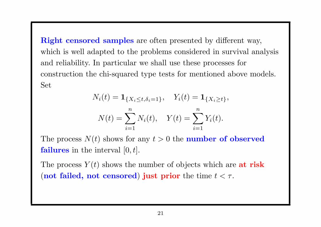
Right censored samples are often presented by different way,

which is well adapted to the problems considered in survival analysis

and reliability. In particular we shall use these processes for

construction the chi-squared type tests for mentioned above models.

Set

Ni(t) = 1{Xi≤t,δi=1}, Yi(t) = 1{Xi≥t},

N(t) =n∑

i=1

Ni(t), Y (t) =n∑

i=1

Yi(t).

The process N(t) shows for any t > 0 the number of observed

failures in the interval [0, t].

The process Y (t) shows the number of objects which are at risk

(not failed, not censored) just prior the time t < τ .

21

It is evident that two above data presentations are equivalent, but

there is a very important advantage of data presentation in terms of

introduced stochastic processes Ni and Yi since they show the

dynamics of failures and censoring history throughout the experiment

and

{Ni(s), Yi(s), 0 ≤ s ≤ t, i = 1, 2, ..., n}

to time t. The notion of history is formalized by introduction of

the notion of filtration generated by stochastic processes Ni and Yi.

22

Suppose that

1) the processes Ni, Yi, zi are observed finite time τ ;

2) survival distribution of all n objects given zi are absolutely

continuous with the survival function Si and the hazard rates λi ;

3) censoring is non informative and the multiplicative

intensities model is verified : the compensators of the counting

processes Ni with respect to the history of the observed

processes are∫ t

0Yiλids, where λi(t, θ) = λ(t, θ, zi).

In this case for non-informative and independent censoring we may

give the following expressions for the likelihood function

L(θ) =n∏

i=1

fδii (Xi, θ)S

1−δii (Xi, θ) G

δii (Xi) g

1−δii (Xi), θ ∈ Θ.

23

Since the problem is to estimate the parameter θ, we can skip the

multipliers which do not depend on this parameter. So under

non-informative censoring the likelihood function has the next form :

L(θ) =n∏

i=1

fδi(Xi, θ)S1−δi(Xi, θ), θ ∈ Θ.

Using the relation fi(t, θ) = λi(t, θ)Si(t, θ) the likelihood function

can be written

L(θ) =

n∏i=1

λδii (Xi, θ)Si(Xi, θ), θ ∈ Θ.

The estimator θ, maximizing the likelihood function L(θ), θ ∈ Θ, is

called maximum likelihood estimator. We denote θ the ML

estimator of θ under H0. We remind that θ = (βT , γT )T .

24

Chi-squared type tests construction

Divide the interval [0, τ ] into k smaller intervals Ij = (aj−1, aj ] with

a0 = 0, ak = τ , and denote by

Uj = N(aj)−N(aj−1)

the number of observed failures in the j-th interval, j = 1, 2...., k.

What is ”expected” number of observed failures in the interval

Ij under the H0 ?

Set λi(t, θ) = λ(t, θ, zi) the hazard function of Ti under zi. Under H0

and regularity conditions the equality

ENi(t) = E

∫ t

0

λi(u, θ)Yi(u)du

holds, since

25

Ni(t)−∫ t

0

λi(u, θ)Yi(u)du

is a martingale of counting process Ni(t). It suggests that we

can ”expect” to observe

ej =

n∑i=1

∫Ij

λi(u, θ)Yi(u)du

failures in the interval Ij ; here θ is the ML estimator of θ under H0.

So a test can be based on the statistic

Z = (Z1, ..., Zk)T , Zj =

1√n(Uj − ej), j = 1, ..., k,

of differences between the numbers of observed and ”expected”

failures in the intervals I1, ..., Ik.

26

3 Asymptotic properties of the test

statistics

To investigate the properties of the statistic Z we need properties of

the stochastic process

Hn(t) =1√n(N(t)−

n∑i=1

∫ t

0

λi(u, θ)Yi(u)du).

To obtain these properties we use the properties of the ML

estimators which are well known.

Conditions A :

θP→ θ0,

1√nℓ(θ0)

d→ Nm(0, i(θ0)),

− 1

nℓ(θ0)

P→ i(θ0),

27

and√n(θ − θ0) = i−1(θ0)

1√nℓ(θ0) + oP (1),

where

ℓ(θ) =n∑

i=1

∫ τ

0

∂

∂θlnλi(u, θ) {dNi(u)− Yi(u)λi(u, θ)du}

is the score function.

28

The conditions A for consistency and asymptotic normality of

the ML estimator θ hold, for example, if conditions VI.1.1 given in

Andersen et al [4] hold. Set

S(0)(t, θ) =

n∑i=1

Yi(t)λi(t, θ), S(1)(t, θ) =

n∑i=1

Yi(t)∂ lnλi(t, θ)

∂θλi(t, θ),

S(2)(t, θ) =

n∑i=1

Yi(t)∂2 lnλi(t, θ)

∂θ2λi(t, θ).

For more details see Andersen, Borgan, Gill and Keiding (1993), Van

der Vaart (1998).

29

Conditions B : There exist a neighborhood θ of θ0 and continuous

bounded on θ × [0, τ ] functions

s(0)(t, θ), s(1)(t, θ) =∂s(0)(t, θ)

∂θ, s(2)(t, θ) =

∂2s(0)(t, θ)

∂θ2,

such that for j = 0, 1, 2

supt∈[0,τ ],θ∈θ

|| 1nS(j)(t, θ)− s(j)(t, θ)|| P→ 0 as n → ∞.

30

The conditions B imply that uniformly for t ∈ [0, τ ]

1

n

n∑i=1

∫ t

0

λi(u, θ0)Yi(u)duP→ A(t),

1

n

n∑i=1

∫ t

0

λi(u, θ0)Yi(u)duP→ C(t),

where A and C are finite quantities.

31

Theorem 3.1 Under the conditions A and B the following

convergence holds :

Hnd→ H on D[0, τ ];

here H is zero mean Gaussian martingale such that for all

0 ≤ s ≤ t

cov(H(s),H(t)) = A(s)− CT (s)I−1(θ0)C(t),

D[0, τ ] is the space of cadlag fonctions with Skorokhod metric.

32

For i = 1, ..., s; j, j′ = 1, ..., k set

Vj = H(aj)−H(aj−1), vjj′ = cov(Vj , Vj′), Aj = A(aj)−A(aj−1),

Cij = Ci(aj)−Ci(aj−1), Cj = (C1j , ..., Cs,j)T , V = [vjj′ ]k×k, C = [Cij ]s×k,

and denote by A a k × k diagonal matrix with the diagonal

elements A1, ..., Ak.

Theorem 3.2 Under conditions A and B

Zd→ Y ∼ Nk(0, V ) as n → ∞,

where

V = A− CT i−1(θ0)C.

33

Set

G = i− CA−1CT .

The formula

V − = A−1 +A−1CTG−CA−1

implies that we need to inverse only diagonal k × k matrix A and

find the general inverse of the s× s matrix G.

34

Theorem 3.3 Under conditions A and B the following estimators of

Aj, Cj, I(θ0) and V are consistent :

Aj = Uj/n, Cj =1

n

n∑i=1

∫Ij

∂

∂θlnλi(u, θ)dNi(u),

and

i =1

n

n∑i=1

∫ τ

0

∂ lnλi(u, θ)

∂θ

(∂ lnλi(u, θ)

∂θ

)T

dNi(u), V = A−CT i−1C.

35

4 Chi-squared goodness-of-fit test

The theorems 1 and 2 imply that a test for the hypothesis H0 can be

based on the statistic

Y 2 = ZT V −Z,

where

V − = A−1 + A−1CT G−CA−1, G = I − CA−1CT .

36

This statistic can be written in the form

Y 2 =k∑

j=1

(Uj − ej)2

Uj+Q,

where

Uj =∑

i:Xi∈Ij

δi, ej =∑

i:Xi>aj−1

[Λ0(aj ∧Xi); γ)− Λ0(aj−1; γ)],

Q = WT G−W,

W = CA−1z = (W1, ...,Ws)T , G = [gll′ ]s×s,

gll′ = ill′ −k∑

j=1

CljCl′jA−1j ,

37

Cj =1

n

∑i:Xi∈Ij

δi∂

∂θlnλi(Xi, θ),

i =1

n

n∑i=1

δi∂ lnλi(Xi, θ)

∂θ

(∂ lnλi(Xi, θ)

∂θ

)T

,

Wl =k∑

j=1

CljA−1j Zj , l, l′ = 1, ..., s.

The limit distribution of the statistic X2 is chi-square with

r = rank(V −) = Tr(V −V ) degrees of freedom. If the matrix G is

non-degenerate then r = k.

38

Test for the hypothesis H0 : the hypothesis is rejected with

approximate significance level α if Y 2 > χ2α(r).

Note that for all examples 1-5 the rank r = k − 1 in the case of

exponential, Weibull, Gompertz baseline distribution, and also for

distribution with hyperbolic baseline hazard function, r = k for

lognormal, loglogistic baseline distribution. In the case of composite

hypothesis of Example 1 and exponential distribution the second

quadratic form in the expression of the test statistic is equal to zero.

39

5 Choice of random grouping intervals

Let us consider choice of the limits of grouping intervals as

random data functions. Define

Ek =

n∑i=1

∫ τ

0

λi(u, θ)Yi(u)du =

n∑i=1

Λi(Xi, θ), Ej =j

kEk, j = 1, ..., k.

So we seek aj to have equal numbers of expected failures (not

necessary integer) in all intervals. So aj verify the equalities

g(aj) = Ej , g(a) =n∑

i=1

∫ a

0

λi(t, θ)Yi(u)du.

40

Denote by X(1) ≤ ... ≤ X(n) the ordered sample from X1, ..., Xn.

Note that the function

g(a) =

n∑i=1

Λi(Xi∧a, θ) =n∑

i=1

[n∑l=i

Λ(l)(a, θ) +

i−1∑l=1

Λ(l)(X(l), θ)

]1[X(i−1),X(i)](a)

is continuous and increasing on [0, τ ] ; here X(0) = 0, and we

understand∑0

l=1 cl = 0. Set

bi =n∑

l=i+1

Λ(l)(X(i), θ) +i∑

l=1

Λ(l)(X(l), θ).

41

If Ej ∈ [bi−1, bi] then aj is the unique solution of the equation

n∑l=i

Λ(l)(aj , θ) +i−1∑l=1

Λ(l)(X(l), θ) = Ej ,

We have 0 < a1 < a2... < ak = τ . Under this choice of the intervals

ej = Ek/k for any j.

Theorem 5.1 Under conditions A and B and random choice of the

endpoints of grouping intervals the limit distribution of the statistic

Y 2 is chi-square with r degrees of freedom.

42

References

42-1

[1] Aalen, O. (1978). Nonparametric inference for the family of counting

processes, Ann. Statist., 6, 701–726.

[2] Akritas, M.G. (1988). Pearson-type goodness-of-fit tests : the univariate

case, J.Amer.Statist.Assoc., 83, 222–230.

[3] Akritas, M.G., Torbeyns, A.F., (1997). Pearson-type goodness-of-fit

tests for regression, Can.J.Statist., 25, 359–374.

[4] Andersen P.K., Borgan O., Gill R.D. and Keiding N. (1993). Statistical

Models Based on Counting Processes, Springer-Verlag : New York.

43

[5] Bagdonavicius, V. and Nikulin, M. (2002).Accelerated Life Models.

Chapman and Hall/CRC, Boca Raton.

[6] Bagdonavicius V., Kruopis, J., Nikulin, M. (2011). Non-parametric tests

for censored data. ISTE&WILEY :London

[7] Billingsley, P. (1968). Convergence of Probability Measures, Wiley : New

York.

[8] Gray, R.J., and Pierce, D.A. (1985). Goodness of fit tests for censored

survival data, Ann. Statist., 13, 552–563.

[9] Greenwood, P., Nikulin, M.S. (1996). A Guide to Chi-squared Testing,

Wiley : New York.

44

[10] Habib, M.G., Thomas, D.R. (1986). Chi-squared goodness-of-fit tests

for randomly censored data, The Annals of Statistics, 14, 759–765.

[11] Hjort, N.L. (1990). Goodness of fit tests in models for life history data

based on cumulative hazard rates, The Annals of Statistics, 18,

1221–1258.

[12] Hollander, M., Pena, E. (1992). Chi-square goodness-of-fit test for

randomly censored data, JASA, 417, 458–463.

[13] Koul, H. (1984). Tests of goodness-of-fit in linear regression, Colloq.

Math. Soc. Janos Bolyai, 45, 279–315.

[14] LeCam, L., Mahan,C., Singh, A. (1983). An extension of a Theorem of

H.Chernoff and E.L.Lehmann. In : Recent advances in statistics,

Academic Press, Orlando, 303–332.

45

[15] Loynes, R.M. (1980). The empirical distribution function of residuals

from generalized regression, Ann. Statist., 8, 285–298.

[16] Mukantseva,L .A. (1977). Testing normality in one-dimensional and

multi-dimensional linear regression, Theory Probab. Appl., 22, 591–602.

[17] Nikulin, M.S. (1973). Chi-square test for continuous distribution with

shift and scale parameters, Theory of Probability and its Application,

19, 559–568.

46

[18] Pierce, D., and Kopecky, K. (1979). Testing goodness of fit for the

distribution of errors in regression models, Biometrika, textbf66, 1–6.

[19] Rao, K.C., and Robson, D.S. (1974). A chi-square statistic for

goodness-of-fit tests within the exponential family, Communications in

Statistics, textbf3, 1139–1153.

47