AF3.1 Use variables in expressions describing geometric quantities (e.g.,
Upload
toby-miles-blackCategory
view
215download
2
Chapter
Describing the Relation between Two Variables
© 2010 Pearson Prentice Hall. All rights reserved
34
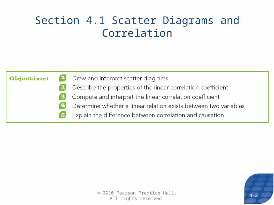
Section 4.1 Scatter Diagrams and Correlation
4-2© 2010 Pearson Prentice Hall. All rights reserved

4-33© 2010 Pearson Prentice Hall. All rights reserved
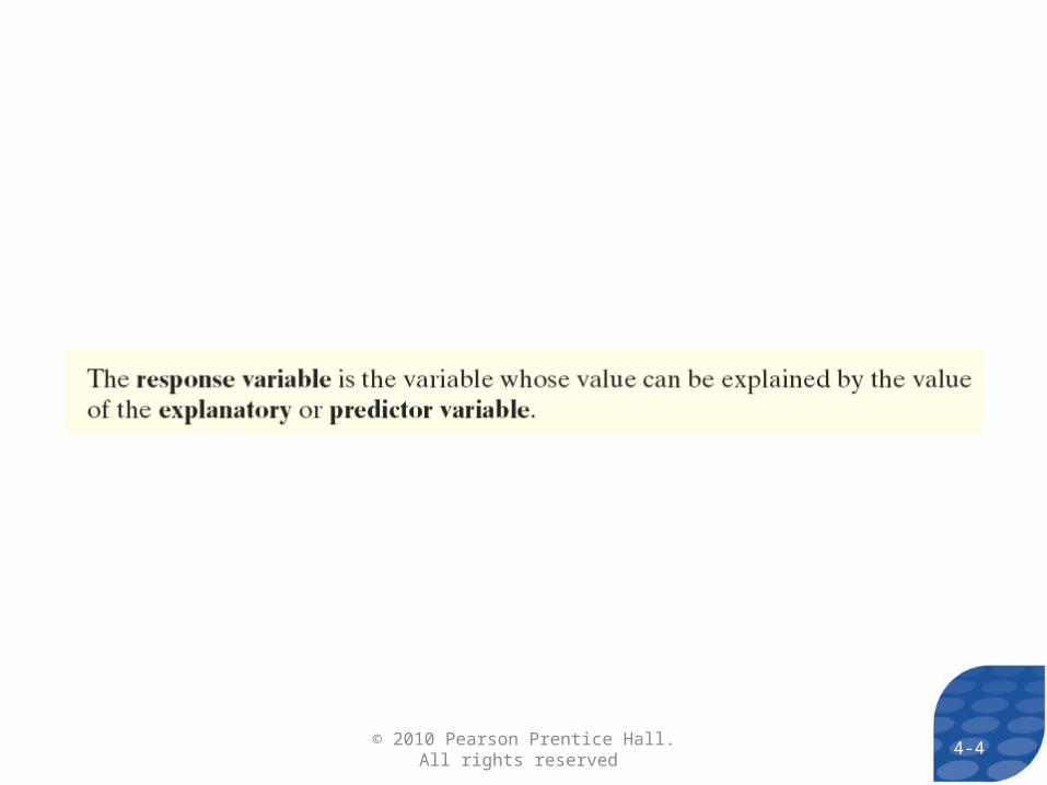
4-4© 2010 Pearson Prentice Hall. All rights reserved
4-55© 2010 Pearson Prentice Hall. All rights reserved
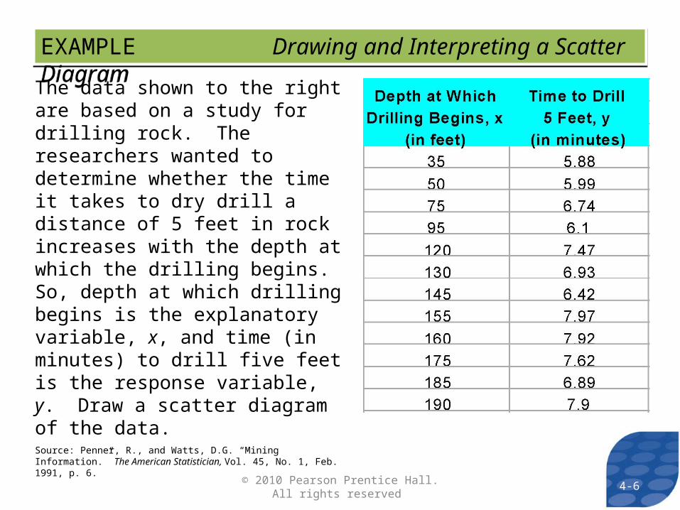
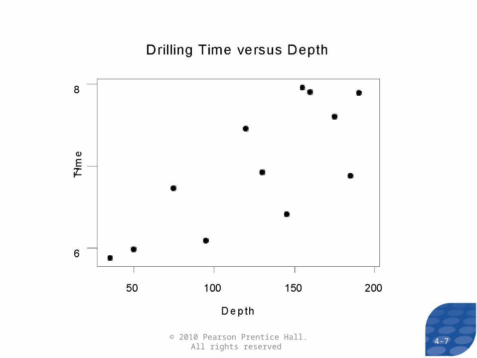
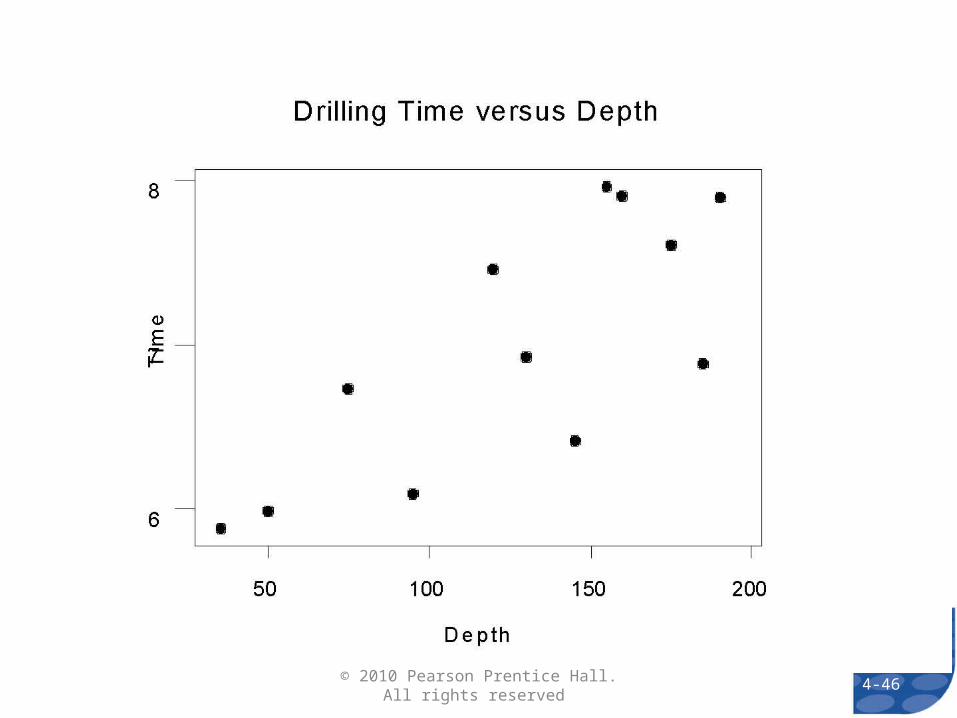
EXAMPLE Drawing and Interpreting a Scatter DiagramEXAMPLE Drawing and Interpreting a Scatter Diagram
The data shown to the right are based on a study for drilling rock. The researchers wanted to determine whether the time it takes to dry drill a distance of 5 feet in rock increases with the depth at which the drilling begins. So, depth at which drilling begins is the explanatory variable, x, and time (in minutes) to drill five feet is the response variable, y. Draw a scatter diagram of the data.Source: Penner, R., and Watts, D.G. “Mining Information.” The American Statistician, Vol. 45, No. 1, Feb. 1991, p. 6.
4-6© 2010 Pearson Prentice Hall. All rights reserved
4-7© 2010 Pearson Prentice Hall. All rights reserved
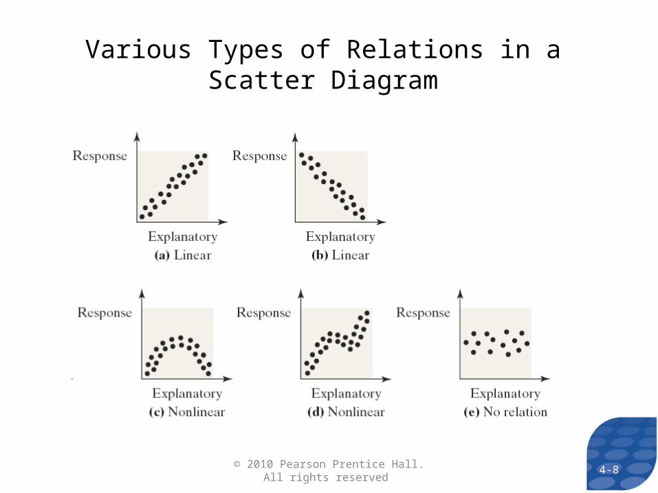
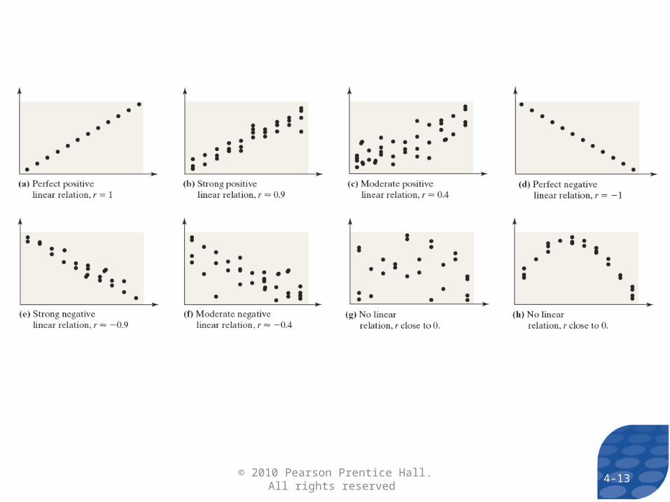
Various Types of Relations in a Scatter Diagram
4-8© 2010 Pearson Prentice Hall. All rights reserved
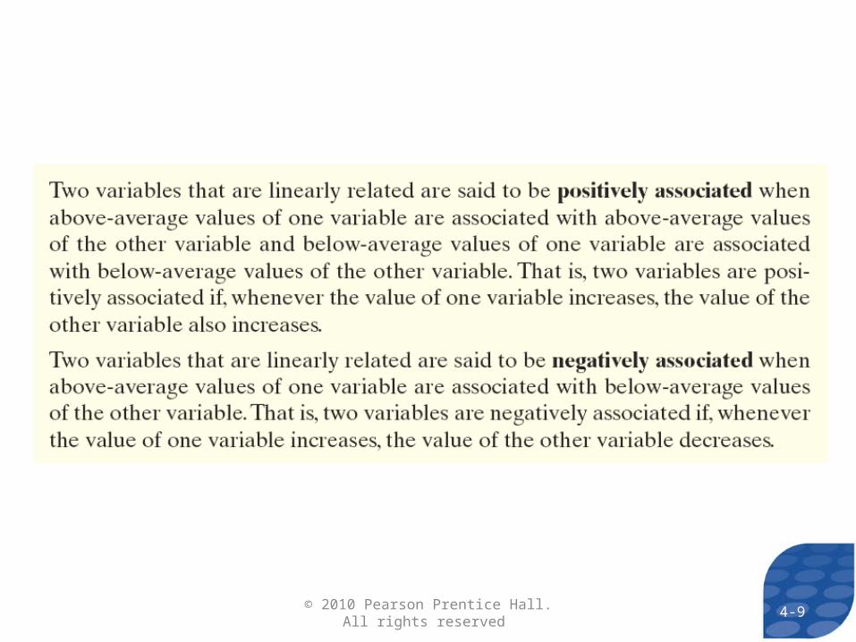
4-9© 2010 Pearson Prentice Hall. All rights reserved
4-10© 2010 Pearson Prentice Hall. All rights reserved
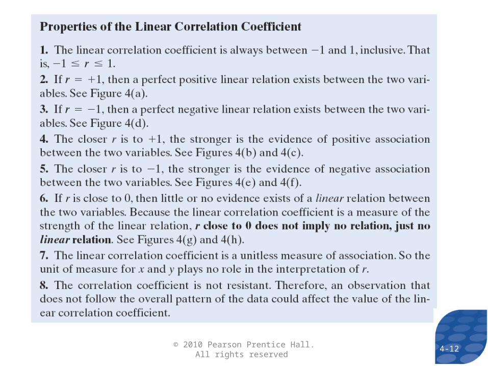
4-11© 2010 Pearson Prentice Hall. All rights reserved
4-12© 2010 Pearson Prentice Hall. All rights reserved
4-13© 2010 Pearson Prentice Hall. All rights reserved
4-14© 2010 Pearson Prentice Hall. All rights reserved

4-15© 2010 Pearson Prentice Hall. All rights reserved
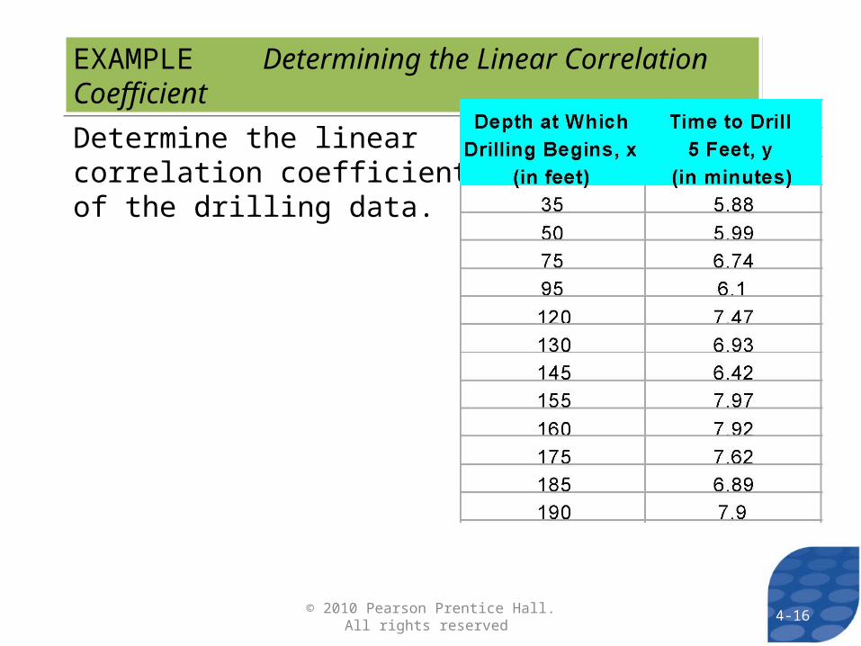
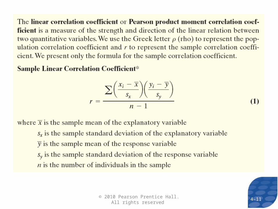
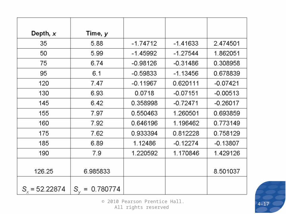
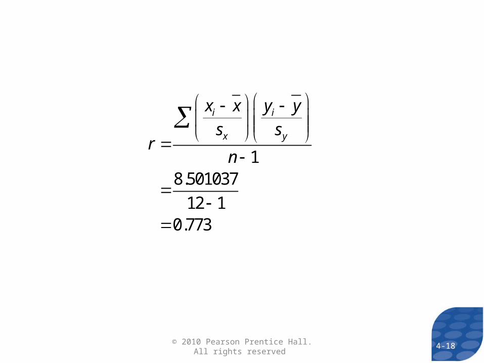
EXAMPLE Determining the Linear Correlation CoefficientEXAMPLE Determining the Linear Correlation Coefficient
Determine the linear correlation coefficient of the drilling data.
4-16© 2010 Pearson Prentice Hall. All rights reserved
4-17© 2010 Pearson Prentice Hall. All rights reserved
18
18.501037
12 10.773
i i
x y
x x y y
s sr
n
4-18© 2010 Pearson Prentice Hall. All rights reserved
194-19© 2010 Pearson Prentice Hall. All rights reserved

204-20© 2010 Pearson Prentice Hall. All rights reserved
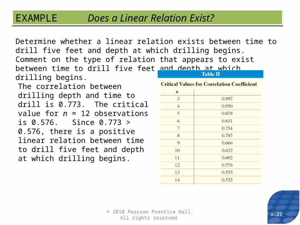
EXAMPLE Does a Linear Relation Exist? EXAMPLE Does a Linear Relation Exist?
Determine whether a linear relation exists between time to drill five feet and depth at which drilling begins. Comment on the type of relation that appears to exist between time to drill five feet and depth at which drilling begins.
The correlation between drilling depth and time to drill is 0.773. The critical value for n = 12 observations is 0.576. Since 0.773 > 0.576, there is a positive linear relation between time to drill five feet and depth at which drilling begins.
214-21© 2010 Pearson Prentice Hall. All rights reserved
224-22© 2010 Pearson Prentice Hall. All rights reserved
23
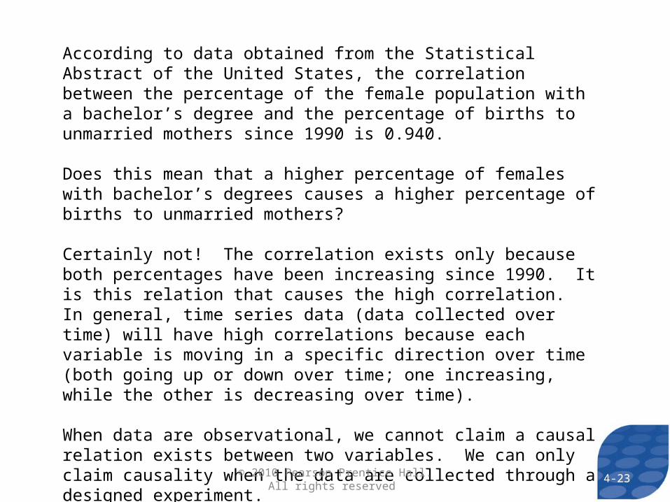
According to data obtained from the Statistical Abstract of the United States, the correlation between the percentage of the female population with a bachelor’s degree and the percentage of births to unmarried mothers since 1990 is 0.940.
Does this mean that a higher percentage of females with bachelor’s degrees causes a higher percentage of births to unmarried mothers?
Certainly not! The correlation exists only because both percentages have been increasing since 1990. It is this relation that causes the high correlation. In general, time series data (data collected over time) will have high correlations because each variable is moving in a specific direction over time (both going up or down over time; one increasing, while the other is decreasing over time).
When data are observational, we cannot claim a causal relation exists between two variables. We can only claim causality when the data are collected through a designed experiment.
4-23© 2010 Pearson Prentice Hall. All rights reserved
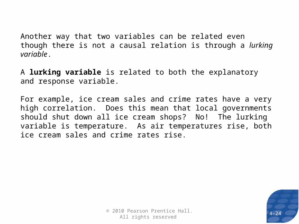
Another way that two variables can be related even though there is not a causal relation is through a lurking variable.
A lurking variable is related to both the explanatory and response variable.
For example, ice cream sales and crime rates have a very high correlation. Does this mean that local governments should shut down all ice cream shops? No! The lurking variable is temperature. As air temperatures rise, both ice cream sales and crime rates rise.
4-24© 2010 Pearson Prentice Hall. All rights reserved
254-25© 2010 Pearson Prentice Hall. All rights reserved
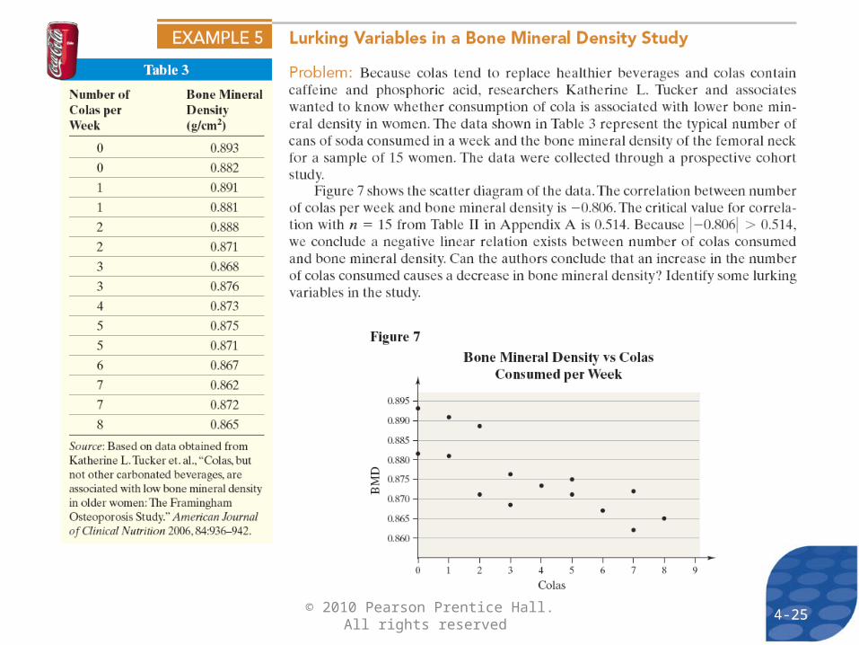
This study is a prospective cohort study, which is an observational study. Therefore, the researchers cannot claim that increased cola consumption causes a decrease in bone mineral density.
Some lurking variables in the study that could confound the results are:
• body mass index• height• smoking• alcohol consumption• calcium intake • physical activity
4-26© 2010 Pearson Prentice Hall. All rights reserved
Section 4.2 Least-squares Regression
274-27© 2010 Pearson Prentice Hall. All rights reserved
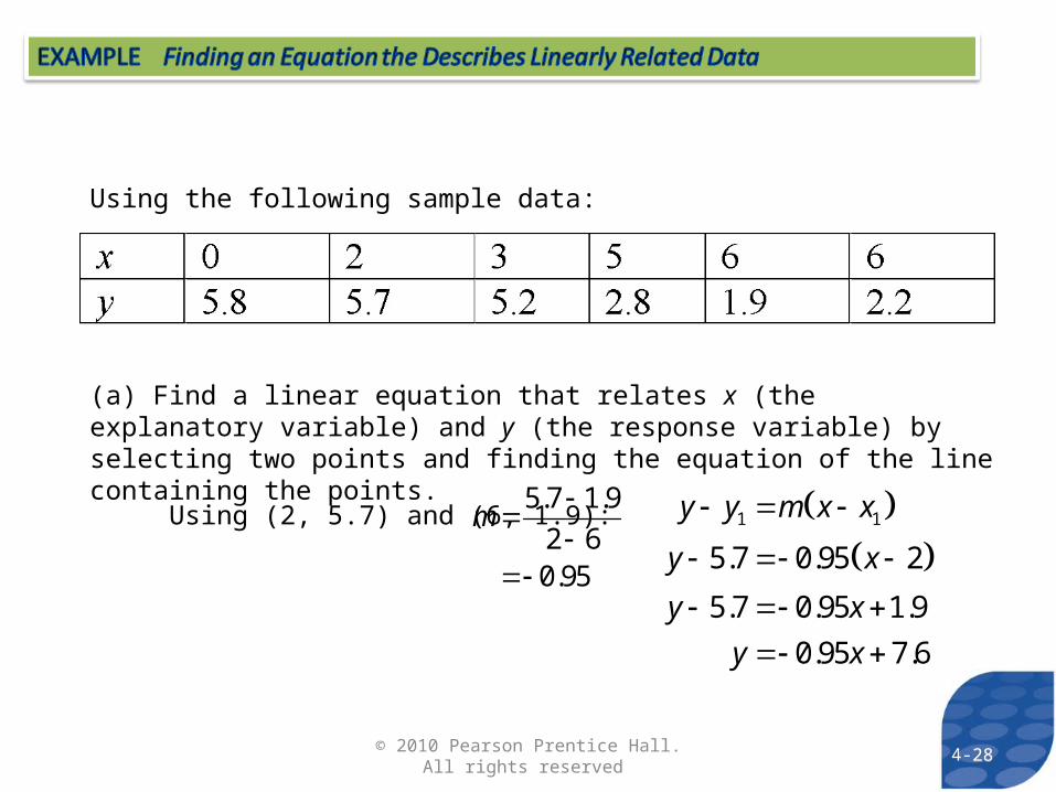
(a) Find a linear equation that relates x (the explanatory variable) and y (the response variable) by selecting two points and finding the equation of the line containing the points.
Using the following sample data:
Using (2, 5.7) and (6, 1.9):5.7 1.9
2 60.95
m
1 1
5.7 0.95 2
5.7 0.95 1.9
0.95 7.6
y y m x x
y x
y x
y x
284-28© 2010 Pearson Prentice Hall. All rights reserved
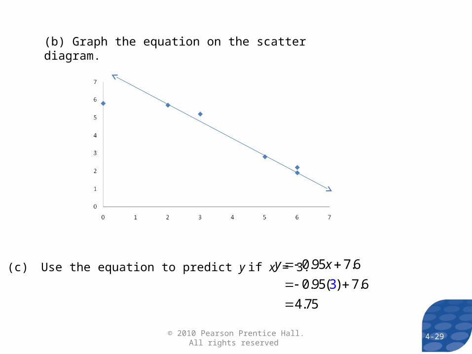
(b) Graph the equation on the scatter diagram.
(c) Use the equation to predict y if x = 3. 0.95 7.6
0. 395( ) 7.6
4.75
y x
4-29© 2010 Pearson Prentice Hall. All rights reserved
4-30© 2010 Pearson Prentice Hall. All rights reserved
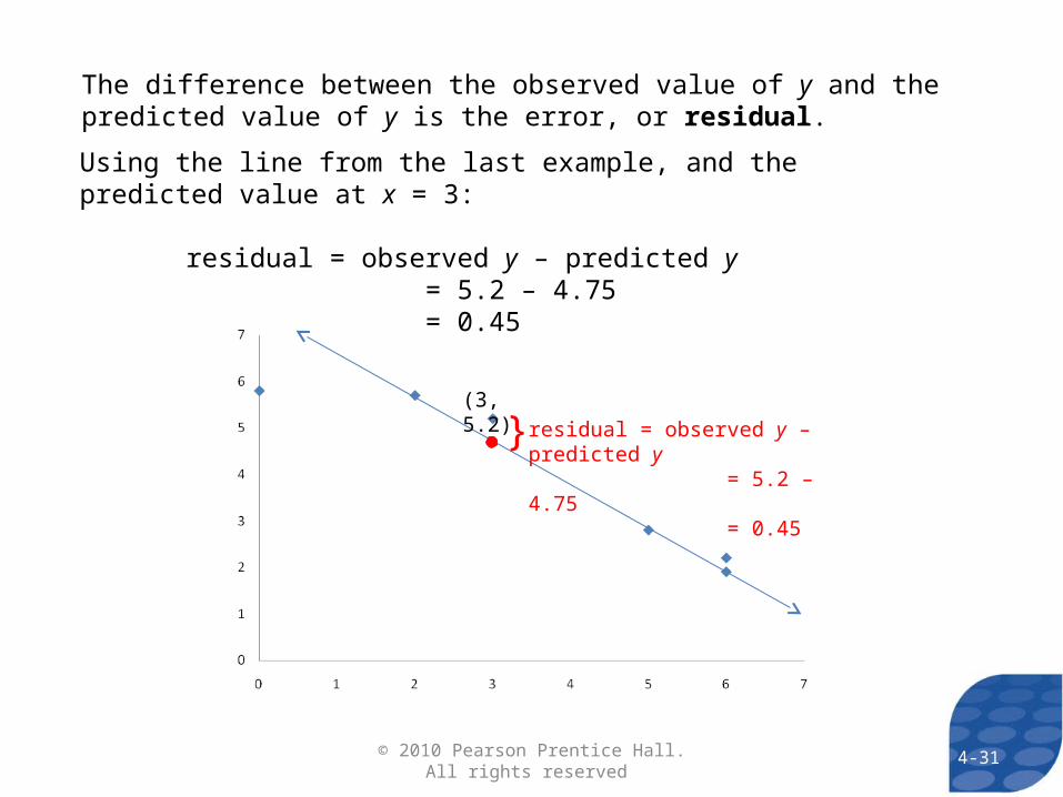
}(3, 5.2)
residual = observed y – predicted y = 5.2 – 4.75 = 0.45
The difference between the observed value of y and the predicted value of y is the error, or residual.
Using the line from the last example, and the predicted value at x = 3:
residual = observed y – predicted y = 5.2 – 4.75 = 0.45
4-31© 2010 Pearson Prentice Hall. All rights reserved
4-32© 2010 Pearson Prentice Hall. All rights reserved
4-33© 2010 Pearson Prentice Hall. All rights reserved
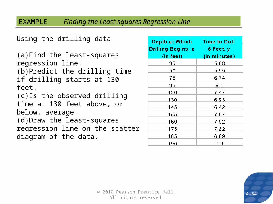
EXAMPLE Finding the Least-squares Regression LineEXAMPLE Finding the Least-squares Regression Line
Using the drilling data
(a)Find the least-squares regression line.(b)Predict the drilling time if drilling starts at 130 feet.(c)Is the observed drilling time at 130 feet above, or below, average.(d)Draw the least-squares regression line on the scatter diagram of the data.
4-34© 2010 Pearson Prentice Hall. All rights reserved
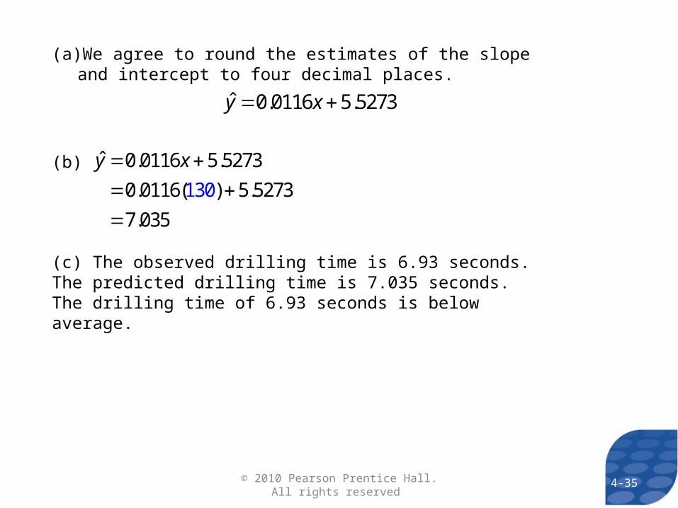
(a) We agree to round the estimates of the slope and intercept to four decimal places.
ˆ 0.0116 5.5273y x
(b) ˆ 0.0116 5.5273
0.0116( ) 5.5273
7. 3
0
5
13
0
y x
(c) The observed drilling time is 6.93 seconds. The predicted drilling time is 7.035 seconds. The drilling time of 6.93 seconds is below average.
4-35© 2010 Pearson Prentice Hall. All rights reserved
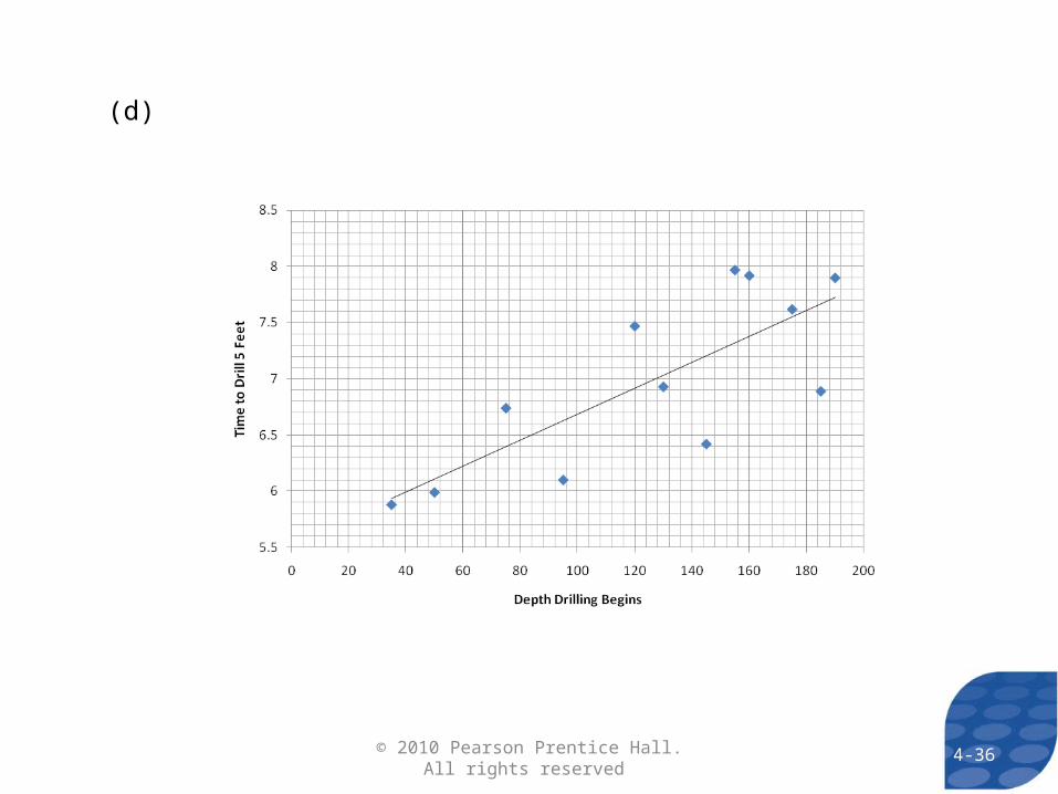
(d)
4-36© 2010 Pearson Prentice Hall. All rights reserved

4-37© 2010 Pearson Prentice Hall. All rights reserved
4-38
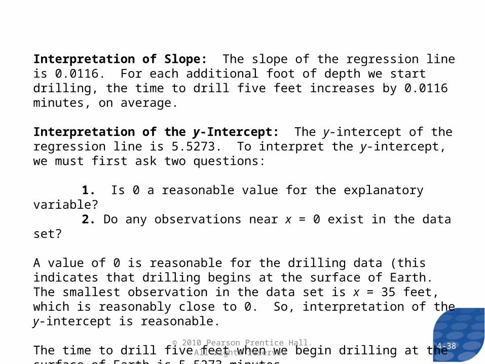
Interpretation of Slope: The slope of the regression line is 0.0116. For each additional foot of depth we start drilling, the time to drill five feet increases by 0.0116 minutes, on average.
Interpretation of the y-Intercept: The y-intercept of the regression line is 5.5273. To interpret the y-intercept, we must first ask two questions:
1. Is 0 a reasonable value for the explanatory variable? 2. Do any observations near x = 0 exist in the data set?
A value of 0 is reasonable for the drilling data (this indicates that drilling begins at the surface of Earth. The smallest observation in the data set is x = 35 feet, which is reasonably close to 0. So, interpretation of the y-intercept is reasonable.
The time to drill five feet when we begin drilling at the surface of Earth is 5.5273 minutes.
© 2010 Pearson Prentice Hall. All rights reserved
If the least-squares regression line is used to make predictions based on values of the explanatory variable that are much larger or much smaller than the observed values, we say the researcher is working outside the scope of the model. Never use a least-squares regression line to make predictions outside the scope of the model because we can’t be sure the linear relation continues to exist.
4-39© 2010 Pearson Prentice Hall. All rights reserved

4-40© 2010 Pearson Prentice Hall. All rights reserved
4-41
To illustrate the fact that the sum of squared residuals for a least-squares regression line is less than the sum of squared residuals for any other line, use the “regression by eye” applet.
© 2010 Pearson Prentice Hall. All rights reserved
Section 4.3 The Coefficient of Determination
4-4242© 2010 Pearson Prentice Hall. All rights reserved

4-4343© 2010 Pearson Prentice Hall. All rights reserved
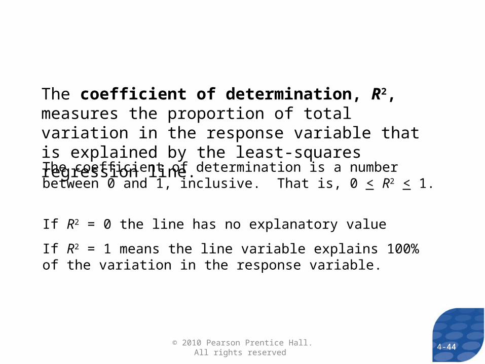
The coefficient of determination, R2, measures the proportion of total variation in the response variable that is explained by the least-squares regression line.
4-44
The coefficient of determination is a number between 0 and 1, inclusive. That is, 0 < R2 < 1.
If R2 = 0 the line has no explanatory value
If R2 = 1 means the line variable explains 100% of the variation in the response variable.
44© 2010 Pearson Prentice Hall. All rights reserved
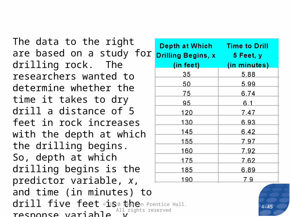
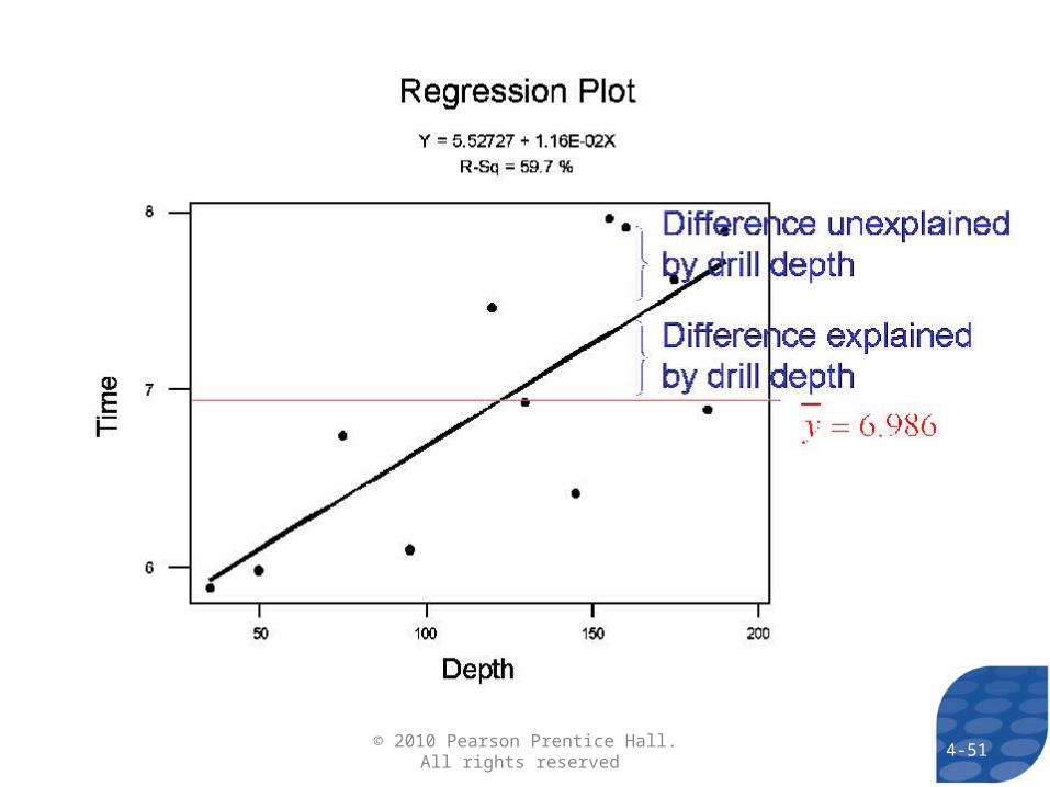
The data to the right are based on a study for drilling rock. The researchers wanted to determine whether the time it takes to dry drill a distance of 5 feet in rock increases with the depth at which the drilling begins. So, depth at which drilling begins is the predictor variable, x, and time (in minutes) to drill five feet is the response variable, y.Source: Penner, R., and Watts, D.G. “Mining Information.” The American Statistician, Vol. 45, No. 1, Feb. 1991, p. 6.
4-4545© 2010 Pearson Prentice Hall. All rights reserved
4-46© 2010 Pearson Prentice Hall. All rights reserved
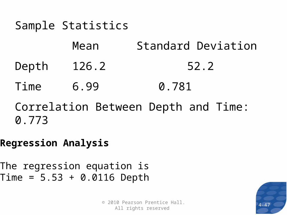
Regression Analysis
The regression equation isTime = 5.53 + 0.0116 Depth
Sample Statistics
Mean Standard Deviation
Depth 126.2 52.2
Time 6.99 0.781
Correlation Between Depth and Time: 0.773
4-47© 2010 Pearson Prentice Hall. All rights reserved
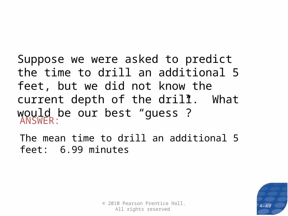
Suppose we were asked to predict the time to drill an additional 5 feet, but we did not know the current depth of the drill. What would be our best “guess”?
4-48© 2010 Pearson Prentice Hall. All rights reserved
Suppose we were asked to predict the time to drill an additional 5 feet, but we did not know the current depth of the drill. What would be our best “guess”?
ANSWER:
The mean time to drill an additional 5 feet: 6.99 minutes
4-49© 2010 Pearson Prentice Hall. All rights reserved
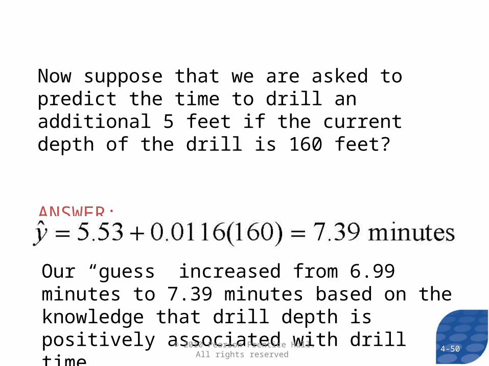
Now suppose that we are asked to predict the time to drill an additional 5 feet if the current depth of the drill is 160 feet?
ANSWER:
Our “guess” increased from 6.99 minutes to 7.39 minutes based on the knowledge that drill depth is positively associated with drill time.
4-50© 2010 Pearson Prentice Hall. All rights reserved
4-51© 2010 Pearson Prentice Hall. All rights reserved
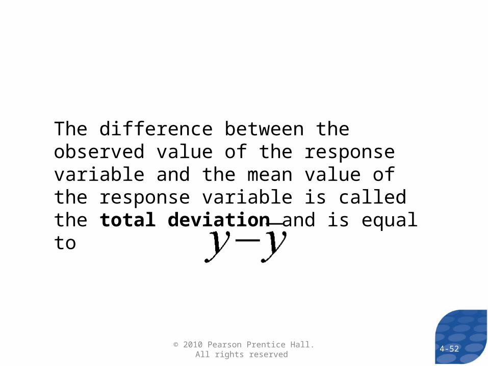
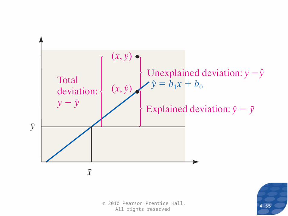
The difference between the observed value of the response variable and the mean value of the response variable is called the total deviation and is equal to
4-52© 2010 Pearson Prentice Hall. All rights reserved
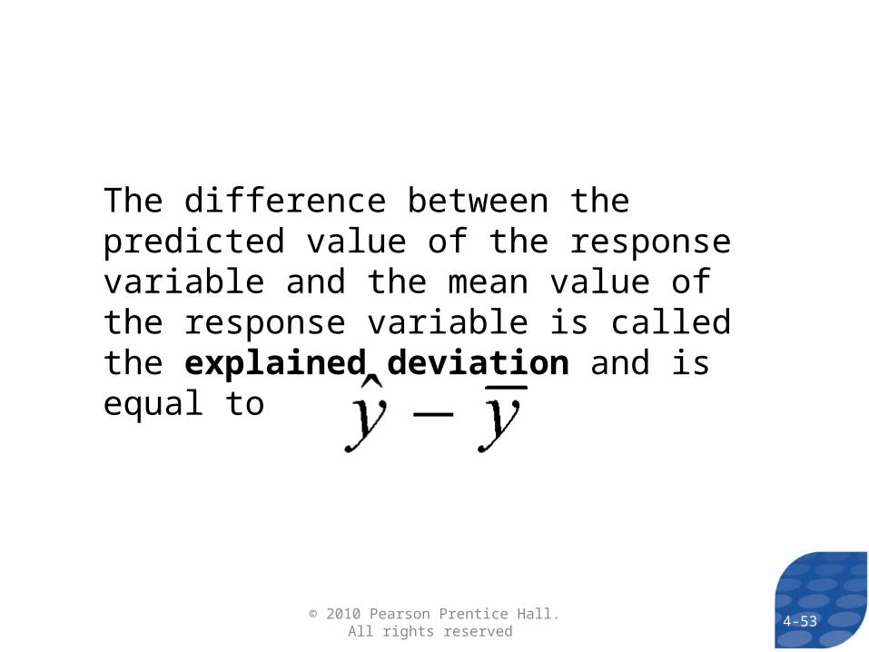
The difference between the predicted value of the response variable and the mean value of the response variable is called the explained deviation and is equal to
4-53© 2010 Pearson Prentice Hall. All rights reserved
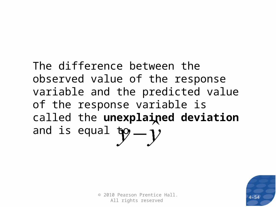
The difference between the observed value of the response variable and the predicted value of the response variable is called the unexplained deviation and is equal to
4-54© 2010 Pearson Prentice Hall. All rights reserved
4-55© 2010 Pearson Prentice Hall. All rights reserved
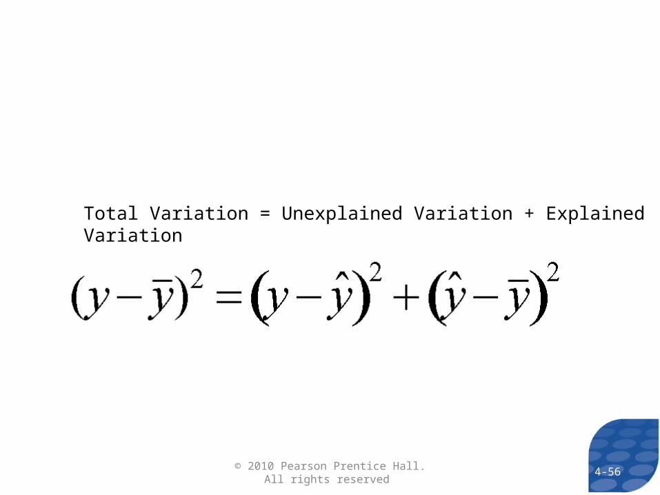
Total Variation = Unexplained Variation + Explained Variation
4-56© 2010 Pearson Prentice Hall. All rights reserved
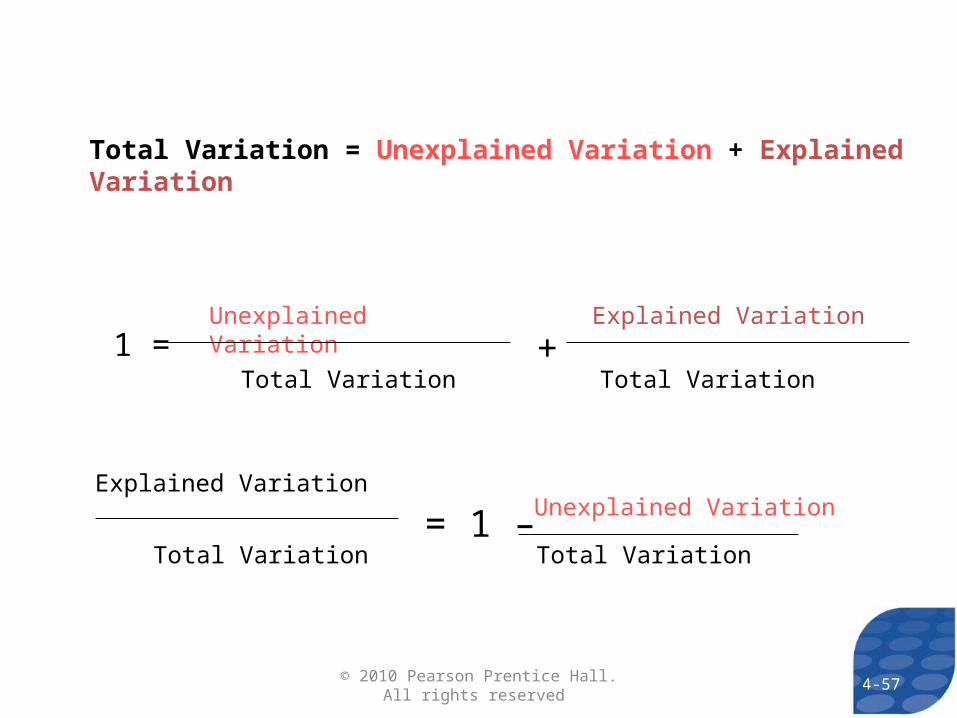
Total Variation = Unexplained Variation + Explained Variation
1 =Unexplained Variation Explained Variation
Unexplained VariationExplained Variation
Total Variation Total Variation
Total VariationTotal Variation
+
= 1 –
4-57© 2010 Pearson Prentice Hall. All rights reserved
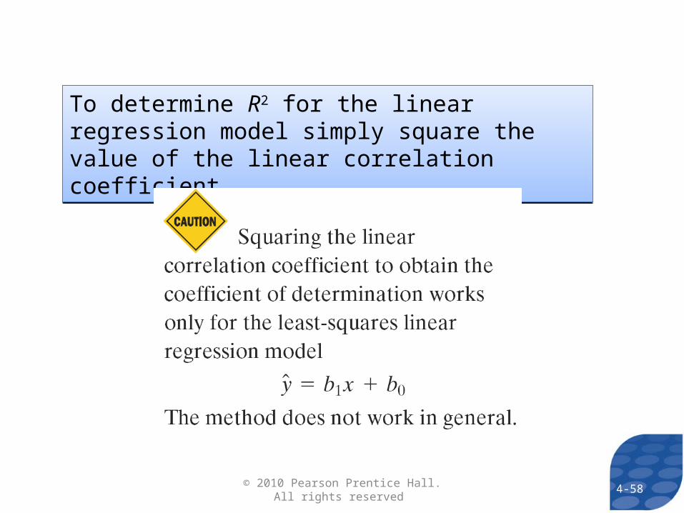
To determine R2 for the linear regression model simply square the value of the linear correlation coefficient.To determine R2 for the linear regression model simply square the value of the linear correlation coefficient.
4-58© 2010 Pearson Prentice Hall. All rights reserved
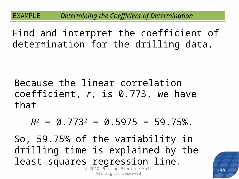
EXAMPLE Determining the Coefficient of DeterminationEXAMPLE Determining the Coefficient of Determination
Find and interpret the coefficient of determination for the drilling data.
Because the linear correlation coefficient, r, is 0.773, we have that
R2 = 0.7732 = 0.5975 = 59.75%.
So, 59.75% of the variability in drilling time is explained by the least-squares regression line.
4-59© 2010 Pearson Prentice Hall. All rights reserved
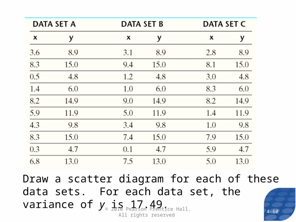
Draw a scatter diagram for each of these data sets. For each data set, the variance of y is 17.49.
4-60© 2010 Pearson Prentice Hall. All rights reserved
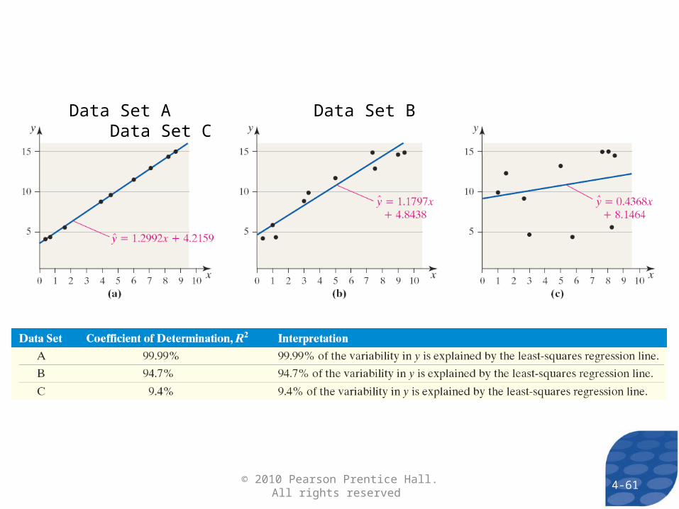
Data Set A Data Set B Data Set C
4-61© 2010 Pearson Prentice Hall. All rights reserved