Describing Quantitative Variables Presentation 3.

Describing Quantitative Describing Quantitative VariablesVariables

Presentation 3

What is a What is a quantitativequantitative variable?variable?

Quantitative variables are recorded as Quantitative variables are recorded as numerical values. They are measurements numerical values. They are measurements or counts taken on each unit in the sample.or counts taken on each unit in the sample.

Consider the following examples:Consider the following examples: 1. Age of a person.1. Age of a person. 2. Number of times a person sees a dentist in a year.2. Number of times a person sees a dentist in a year. 3. Weight of a dog. 3. Weight of a dog. 4. Number of credits a student takes in a semester.4. Number of credits a student takes in a semester.

Note:Note: Quantitative variables can be either Quantitative variables can be either continuous or discrete. Continuous variables can take continuous or discrete. Continuous variables can take on any numerical value in a range. Discrete on any numerical value in a range. Discrete variables can take on only fixed valuesvariables can take on only fixed values. .

What is not a quantitative What is not a quantitative variable…variable…

Numbers that represent categories are Numbers that represent categories are NOT quantitative variables.NOT quantitative variables.

Your SSN# for example is a label, not a Your SSN# for example is a label, not a measurement.measurement.

Helpful Hint:Helpful Hint: When considering if something is a When considering if something is a quantitative variable consider if an average of the quantitative variable consider if an average of the variable is meaningful. The average height in a variable is meaningful. The average height in a sample would certainly be of interest. The average sample would certainly be of interest. The average SSN# would not.SSN# would not.

The Four Features of Quantitative The Four Features of Quantitative DataData

Location:Location: What is the center or average What is the center or average value?value?

Spread:Spread: What is the spread or variability What is the spread or variability of the values? Do they fall closely around of the values? Do they fall closely around the center or far apart?the center or far apart?

Shape:Shape: What is the shape of the data? What is the shape of the data? Bell-shaped or skewed? Symmetric?Bell-shaped or skewed? Symmetric?

Outliers:Outliers: Are there any extreme or Are there any extreme or unusual observations?unusual observations?

Tools to Describe Quantitative Tools to Describe Quantitative Data Data

Five Number Summary:Five Number Summary: Table that consists of Table that consists of the minimum, first and third quartiles, median, the minimum, first and third quartiles, median, and the maximum values of a sample. Used to and the maximum values of a sample. Used to describe both the center and spread of values.describe both the center and spread of values.

Graphs:Graphs: Dotplots, Histograms, and Boxplots are Dotplots, Histograms, and Boxplots are useful to illustrate location, spread, and shape of useful to illustrate location, spread, and shape of data, as well as identify outliers.data, as well as identify outliers.

Numerical Summaries:Numerical Summaries: All five members of the All five members of the five number summaryfive number summary, in addition to the sample , in addition to the sample mean and standard deviation.mean and standard deviation.

How to Construct a Five Number How to Construct a Five Number Summary:Summary:

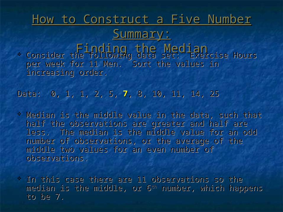
Finding the MedianFinding the Median Consider the following data set: Exercise Hours per Consider the following data set: Exercise Hours per

week for 11 Men. Sort the values in increasing order. week for 11 Men. Sort the values in increasing order.

Data: 0, 1, 1, 2, 5, Data: 0, 1, 1, 2, 5, 77, 8, 10, 11, 14, 25, 8, 10, 11, 14, 25

Median is the middle value in the data, such that half Median is the middle value in the data, such that half the observations are greater and half are less. The the observations are greater and half are less. The median is the middle value for an odd number of median is the middle value for an odd number of observations, or the average of the middle two observations, or the average of the middle two values for an even number of observations.values for an even number of observations.

In this case there are 11 observations so the median In this case there are 11 observations so the median is the middle, or 6is the middle, or 6thth number, which happens to be 7. number, which happens to be 7.

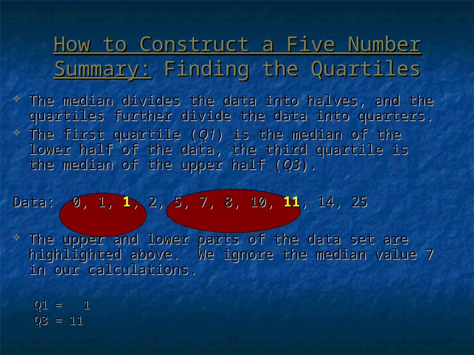
The median divides the data into halves, and the The median divides the data into halves, and the quartiles further divide the data into quarters.quartiles further divide the data into quarters.

The first quartile (The first quartile (Q1Q1) is the median of the lower half ) is the median of the lower half of the data, the third quartile is the median of the of the data, the third quartile is the median of the upper half (upper half (Q3Q3).).

Data: 0, 1, Data: 0, 1, 11, 2, 5, 7, 8, 10, , 2, 5, 7, 8, 10, 1111, 14, 25, 14, 25

The upper and lower parts of the data set are The upper and lower parts of the data set are highlighted above. We ignore the median value 7 in highlighted above. We ignore the median value 7 in our calculations.our calculations.

Q1 = 1Q1 = 1Q3 = 11Q3 = 11

How to Construct a Five Number How to Construct a Five Number Summary:Summary: Finding the Quartiles Finding the Quartiles

How to Construct a Five Number How to Construct a Five Number Summary:Summary: Min and Max Min and Max

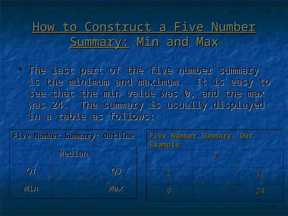
The last part of the five number summary is the The last part of the five number summary is the minimum and maximum. It is easy to see that minimum and maximum. It is easy to see that the min value was 0, and the max was 24. The the min value was 0, and the max was 24. The summary is usually displayed in a table as summary is usually displayed in a table as follows:follows:

Five Number Summary: Five Number Summary: OutlineOutline

MedianMedian

Q1Q1 Q3Q3

MinMin MaxMax

Five Number Summary: Our Five Number Summary: Our ExampleExample

77

11 1111

00 2424

Interpreting the Five Number SummaryInterpreting the Five Number Summary

SexSexHeigHeig

hthtHand Hand

SpanSpanFemaleFemale 6868 21.521.5

MaleMale 7171 23.523.5

MaleMale 7373 22.522.5

FemaleFemale 6464 1818

MaleMale 6868 23.523.5


MaleMale 7373 2323

MaleMale 7575 24.524.5


…… …… ……

Min Q1 Median Q3

Max

25% 25%25% 25%

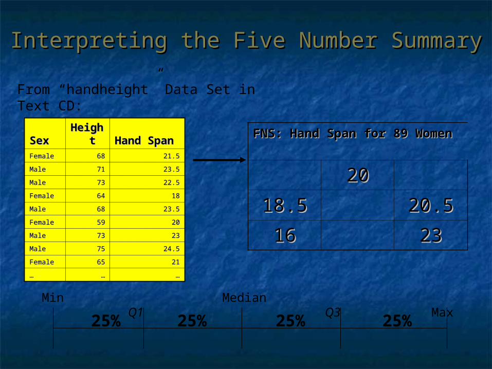
FNS: Hand Span for 89 FNS: Hand Span for 89 WomenWomen

2020

18.518.5 20.520.5

1616 2323

From “handheight” Data Set in Text CD:

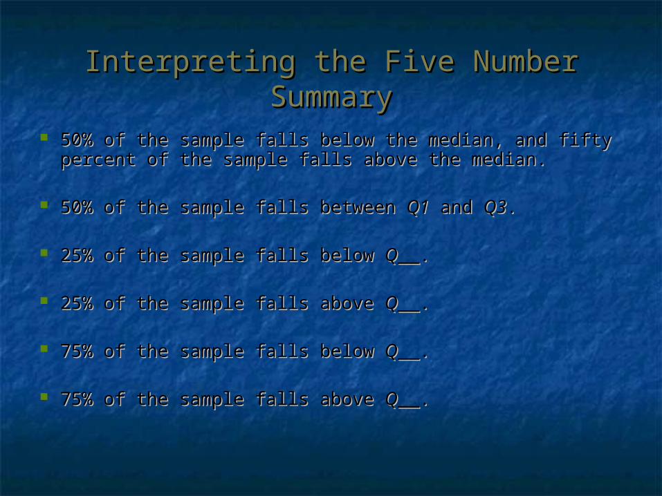
Interpreting the Five Number SummaryInterpreting the Five Number Summary

50% of the sample falls below the median, and fifty 50% of the sample falls below the median, and fifty percent of the sample falls above the median.percent of the sample falls above the median.

50% of the sample falls between 50% of the sample falls between Q1Q1 and and Q3Q3..

25% of the sample falls below 25% of the sample falls below QQ__.__.

25% of the sample falls above 25% of the sample falls above QQ__.__.

75% of the sample falls below 75% of the sample falls below QQ__.__.

75% of the sample falls above 75% of the sample falls above QQ__.__.

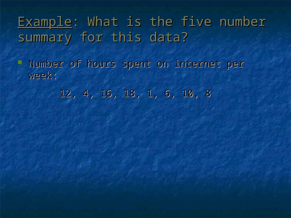
ExampleExample: What is the five number : What is the five number summary for this data?summary for this data?

Number of hours spent on internet per week:Number of hours spent on internet per week:

12, 4, 16, 18, 1, 6, 10, 8 12, 4, 16, 18, 1, 6, 10, 8

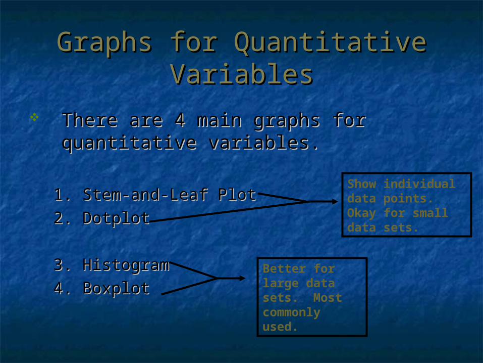
Graphs for Quantitative Graphs for Quantitative VariablesVariables

There are 4 main graphs for quantitative There are 4 main graphs for quantitative variables.variables.

1. Stem-and-Leaf Plot1. Stem-and-Leaf Plot

2. Dotplot2. Dotplot

3. Histogram3. Histogram

4. Boxplot4. Boxplot

Show individual data points. Okay for small data sets.

Better for large data sets. Most commonly used.

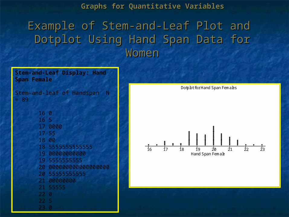
Example of Stem-and-Leaf Plot and Dotplot Example of Stem-and-Leaf Plot and Dotplot Using Hand Span Data for WomenUsing Hand Span Data for Women

Stem-and-Leaf Display: Hand Span Female

Stem-and-leaf of Handspan N = 89

16 0 16 5 17 0000 17 55 18 00 18 5555555555555 19 00000000000 19 5555555555 20 000000000000000000 20 55555555555 21 00000000 21 55555 22 0 22 5 23 0

16 17 18 19 20 21 22 23Hand Span Female

Dotplot for Hand Span Females

Graphs for Quantitative VariablesGraphs for Quantitative Variables

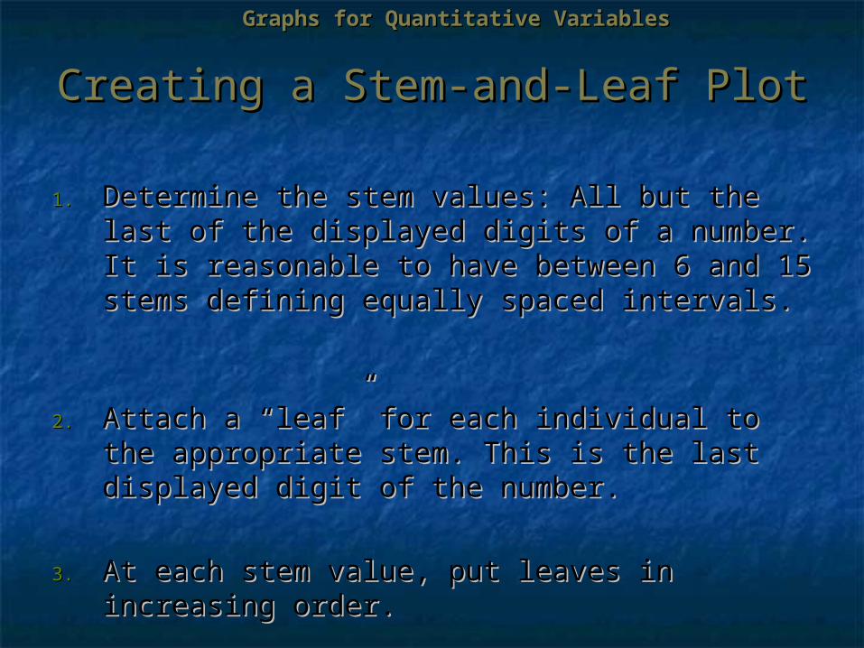
Creating a Stem-and-Leaf PlotCreating a Stem-and-Leaf Plot

1.1. Determine the stem values: All but the last of Determine the stem values: All but the last of the displayed digits of a number. It is reasonable the displayed digits of a number. It is reasonable to have between 6 and 15 stems defining to have between 6 and 15 stems defining equally spaced intervals. equally spaced intervals.

2.2. Attach a “leaf” for each individual to the Attach a “leaf” for each individual to the appropriate stem. This is the last displayed digit appropriate stem. This is the last displayed digit of the number.of the number.

3.3. At each stem value, put leaves in increasing At each stem value, put leaves in increasing order.order.


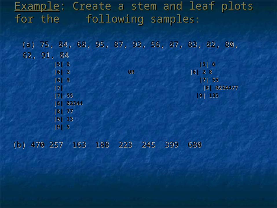
ExampleExample: Create a stem and leaf plots for : Create a stem and leaf plots for the following samplethe following samples:s:

(a) 75, 84, 68, 95, 87, 93, 56, 87, 83, 82, 80, 62, 91, 84(a) 75, 84, 68, 95, 87, 93, 56, 87, 83, 82, 80, 62, 91, 84|5| 6 |5| 6|5| 6 |5| 6

|6| 2 OR |6| 2 8|6| 2 OR |6| 2 8

|6| 8 |7| 55|6| 8 |7| 55

|7| |8| 0234477|7| |8| 0234477

|7| 55 |9| 135|7| 55 |9| 135

|8| 02344|8| 02344

|8| 77|8| 77

|9| 13|9| 13

|9| 5|9| 5

(b) 470 257 163 188 223 245 399 680(b) 470 257 163 188 223 245 399 680

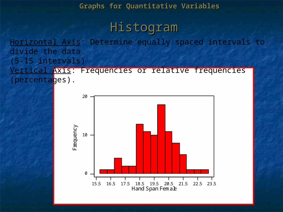
HistogramHistogram

15.5 16.5 17.5 18.5 19.5 20.5 21.5 22.5 23.5

0

10

20

Hand Span Female

Freq

uenc

y

Horizontal Axis: Determine equally spaced intervals to divide the data. (5-15 intervals)Vertical Axis: Frequencies or relative frequencies (percentages).


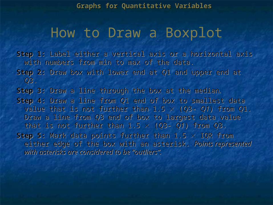
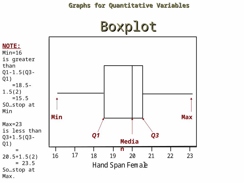
How to Draw a Boxplot

Step 1: Step 1: Label either a vertical axis or a horizontal axis Label either a vertical axis or a horizontal axis with numbers from min to max of the data.with numbers from min to max of the data.

Step 2: Step 2: Draw box with lower end at Draw box with lower end at QQ1 and upper end at 1 and upper end at QQ3.3.

Step 3: Step 3: Draw a line through the box at the medianDraw a line through the box at the median..

Step 4: Step 4: Draw a line from Draw a line from QQ1 end of box to smallest data 1 end of box to smallest data value that is not further than 1.5 value that is not further than 1.5 ( (QQ3- 3- Q1Q1) from ) from QQ1. 1. Draw a line from Draw a line from QQ3 end of box to largest data value 3 end of box to largest data value that is not further than 1.5 that is not further than 1.5 ( (QQ3- 3- Q1Q1) from ) from QQ3.3.

Step 5: Step 5: Mark data points further than 1.5 Mark data points further than 1.5 IQR from either IQR from either edge of the box with an asterisk. edge of the box with an asterisk. Points represented with Points represented with asterisks are considered to be “outliers”.asterisks are considered to be “outliers”.


2322212019181716

Hand Span Female

BoxplotBoxplot

Min

Q1Median

Q3

Max


NOTE:Min=16 is greater thanQ1-1.5(Q3-Q1) =18.5-1.5(2) =15.5SO…stop at Min

Max=23 is less thanQ3+1.5(Q3-Q1) = 20.5+1.5(2) = 23.5So…stop at Max.

807060

30

20

10

0

Height Male (inches)

Fre

que

ncy

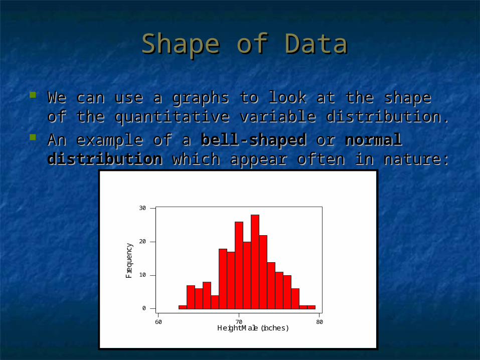
Shape of DataShape of Data

We can use a graphs to look at the shape of the We can use a graphs to look at the shape of the quantitative variable distribution.quantitative variable distribution.

An example of a An example of a bell-shapedbell-shaped or or normal normal distributiondistribution which appear often in nature: which appear often in nature:

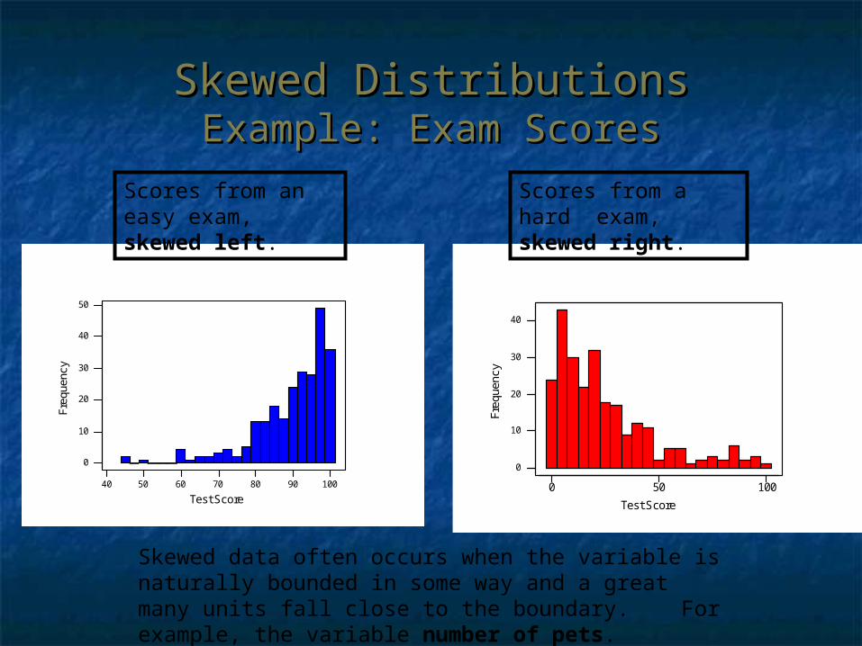
Skewed DistributionsSkewed DistributionsExample: Exam ScoresExample: Exam Scores

40 50 60 70 80 90 100

0

10

20

30

40

50

Test Score

Freq

uenc

y

0 50 100

0

10

20

30

40

Test ScoreFr

eque

ncy

Scores from an easy exam, skewed left.

Scores from a hard exam, skewed right.

Skewed data often occurs when the variable is naturally bounded in some way and a great many units fall close to the boundary. For example, the variable number of pets.

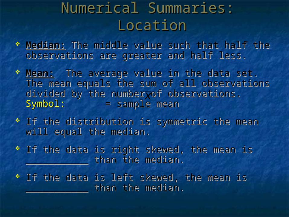
Numerical Summaries: LocationNumerical Summaries: Location

Median:Median: The middle value such that half the The middle value such that half the observations are greater and half less.observations are greater and half less.

Mean:Mean: The average value in the data set. The The average value in the data set. The mean equals the sum of all observations divided mean equals the sum of all observations divided by the number of observations. by the number of observations. Symbol:Symbol: = = sample meansample mean

If the distribution is symmetric the mean will If the distribution is symmetric the mean will equal the median.equal the median.

If the data is right skewed, the mean is ___________ If the data is right skewed, the mean is ___________ than the median.than the median.

If the data is left skewed, the mean is ___________ If the data is left skewed, the mean is ___________ than the median.than the median.

x

Numerical Summaries: SpreadNumerical Summaries: Spread

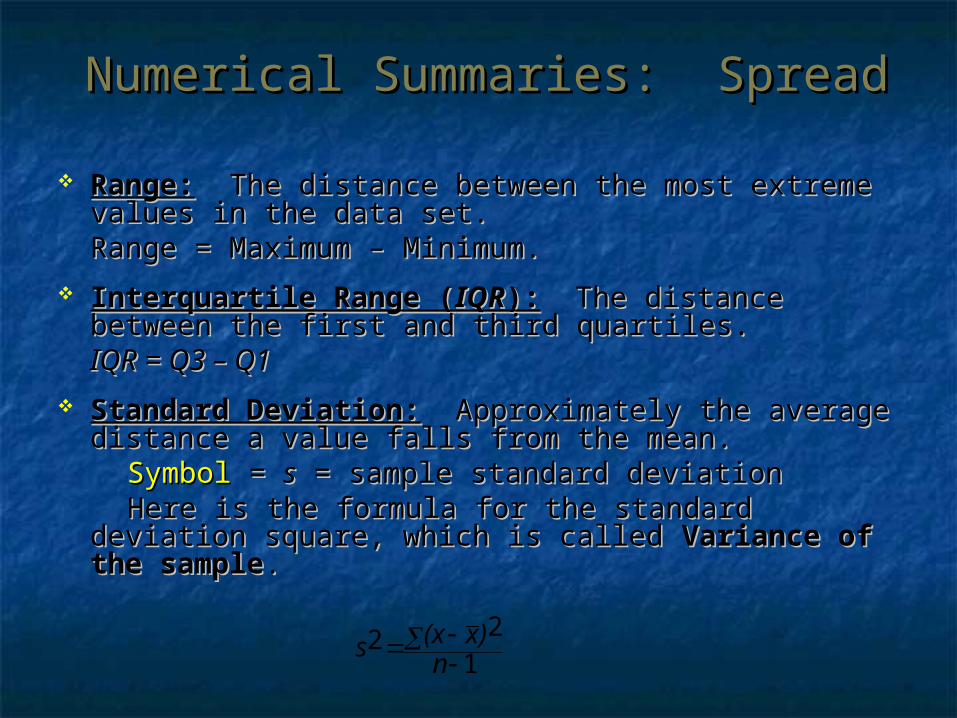
Range:Range: The distance between the most extreme The distance between the most extreme values in the data set. values in the data set. Range = Maximum – Minimum.Range = Maximum – Minimum.

Interquartile Range (Interquartile Range (IQRIQR):): The distance The distance between the first and third quartiles. between the first and third quartiles. IQR = Q3 – Q1IQR = Q3 – Q1

Standard Deviation:Standard Deviation: Approximately the Approximately the average distance a value falls from the mean. average distance a value falls from the mean.

SymbolSymbol = = ss = sample standard deviation = sample standard deviation Here is the formula for the standard deviation Here is the formula for the standard deviation

square, which is called square, which is called Variance of the sampleVariance of the sample..

122

n

)x(xs

Example – Calculate Variance by handExample – Calculate Variance by hand

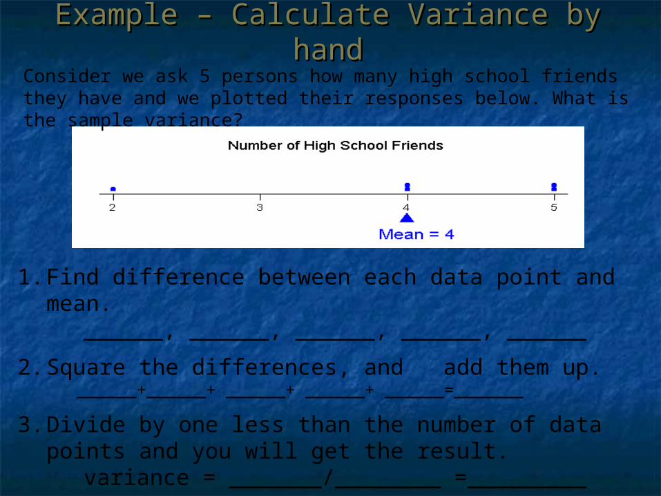
1. Find difference between each data point and mean. ______, ______, ______, ______, ______

2. Square the differences, and add them up. ______+______+ ______+ ______+ ______=_______

3. Divide by one less than the number of data points and you will get the result.

variance = _______/________ =_________

Consider we ask 5 persons how many high school friends they have and we plotted their responses below. What is the sample variance?

OutliersOutliersDefinition: An outlier is a data point that is not

consistent with the bulk of the data.

Possible Reasons for Outliers:

1. An error was made while taking the measurement or entering it into the computer.

2. The individual belongs to a different group than the bulk of individuals measured.

3. The outlier is a legitimate, though extreme data value.

Identifying OutliersIdentifying Outliers

8277726762

Height Male

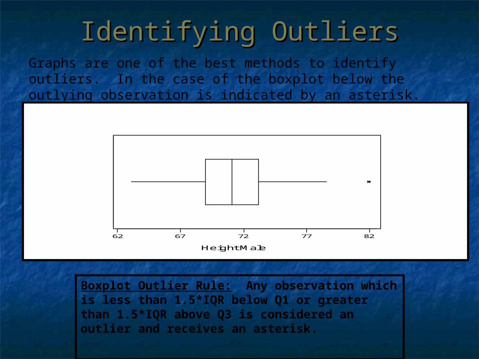
Graphs are one of the best methods to identify outliers. In the case of the boxplot below the outlying observation is indicated by an asterisk.

Boxplot Outlier Rule: Any observation which is less than 1.5*IQR below Q1 or greater than 1.5*IQR above Q3 is considered an outlier and receives an asterisk.

Resistant StatisticsResistant Statistics

Resistant statistics are those that are Resistant statistics are those that are “resistant” to the influence of outliers.“resistant” to the influence of outliers.

Resistant:Resistant: Median, Median, IQRIQR

Non-Resistant:Non-Resistant: Mean, Std. Deviation, and Mean, Std. Deviation, and RangeRange

The most appropriate measure of variability depends on …

the shape of the data’s distribution.

If data are symmetric, with no serious If data are symmetric, with no serious outliers, use range and standard outliers, use range and standard deviation.deviation.

If data are skewed, and/or have serious If data are skewed, and/or have serious outliers, use outliers, use IQRIQR..

The Empirical RuleThe Empirical Rule

The Empirical Rule states that for any bell-The Empirical Rule states that for any bell-shaped curve, approximatelyshaped curve, approximately

68% of the values fall within 1 standard 68% of the values fall within 1 standard deviation of the mean in either direction. deviation of the mean in either direction.

(i.e. plus or minus (i.e. plus or minus ss)) 95% of the values fall within 2 standard 95% of the values fall within 2 standard

deviation of the mean in either direction. deviation of the mean in either direction. 99.7% of the values fall within 3 standard 99.7% of the values fall within 3 standard

deviation of the mean in either direction. deviation of the mean in either direction.

x

Describing Quantitative Variables Presentation 3.

Documents

Transcript of Describing Quantitative Variables Presentation 3.